Embed Size (px)
Citation preview

8/6/2019 umi-umd-3786
http://slidepdf.com/reader/full/umi-umd-3786 1/146
ABSTRACT
Title of Thesis: EXPERIMENTAL CHARACTERIZATION OFACOUSTIC WAVE PROPAGATION
THROUGH A SUPERSONIC DUCTED FLOW
Gregory Carlton Stamp, Master of Science, 2006
Directed By: Associate Professor Dr. Kenneth H. Yu
Department of Aerospace Engineering
In scramjet combustors, if pressure waves could propagate upstream through subsonic
boundary layer flow, it would set up an acoustic feedback mechanism that could lead to self-
sustained combustion instability. To investigate the possibility of upstream wave propagation,
non-reacting supersonic flow experiments were conducted in a specially-designed supersonic
flow duct, which simulated the internal flow path of a dual-mode scramjet combustor.
Furthermore, to experimentally simulate combustion instability, large-amplitude pressure
oscillations were created by passively exciting the exhaust jet flow using screech mechanism,
which resulted in large-amplitude pressure oscillations with dominant frequencies ranging
between 2.7kHZ and 4.2kHz. Then, the acoustic signal was tracked along the supersonic flow
duct using four high-frequency-response Kistler pressure transducers that were flush-mounted at
the combustor and isolator walls. Schlieren visualization was conducted to characterize the
internal supersonic flow field, and an analytical approach was used to estimate the turbulent
boundary layer growth and displacement thickness. Ten sets of experiments were conducted at
various stagnation pressure values ranging from 35psi to 125psi, and four sets of experiments

8/6/2019 umi-umd-3786
http://slidepdf.com/reader/full/umi-umd-3786 2/146
where strong resonances were observed were repeated over ten separate runs for reproducibility.
Fast Fourier Transform was used to quantify the changes in pressure oscillation amplitude in
each case. The results conclusively show that the downstream disturbances were propagating
upstream, and they were being attenuated at different rates depending on flow conditions and
duct geometry. Possible reasons for this new phenomenon were examined and discussed.
8/6/2019 umi-umd-3786
http://slidepdf.com/reader/full/umi-umd-3786 3/146
EXPERIMENTAL CHARACTERIZATION OF ACOUSTIC WAVE
PROPAGATION THROUGH A SUPERSONIC DUCTED FLOW
By
Gregory Carlton Stamp
Thesis submitted to the Faculty of the Graduate School of the
University of Maryland, College Park, in partial fulfillment
of the requirements for the degree of
Master of Science2006
Advisory Committee:
Dr. Kenneth Yu, ChairDr. Christopher Cadou
Dr. James Baeder

8/6/2019 umi-umd-3786
http://slidepdf.com/reader/full/umi-umd-3786 4/146
© Copyright by
Gregory Carlton Stamp
2006

8/6/2019 umi-umd-3786
http://slidepdf.com/reader/full/umi-umd-3786 5/146
ii
Dedication
This thesis is dedicated to my father, Clive Oliver Stamp, who has given me the desire
and passion for learning as well as the vision to see and believe in the possibilities in life.
He has given me the courage to challenge conventional thinking and create pathways that
were considered to be impossible. These timeless intangibles are, in essence, the critical
reasons for my motivated and assiduous effort in pursuing this scholarly work.

8/6/2019 umi-umd-3786
http://slidepdf.com/reader/full/umi-umd-3786 6/146
iii
Acknowledgements
I would like to thank our benevolent Creator for the Divine guidance and strength to
pursue this endeavor, because without Him nothing is possible. I’m eternally grateful to
my advisor, Dr. Kenneth Yu, for his invaluable advice and support of this research. I
would like to thank also the other members of this committee, Dr. Christopher Cadou and
Dr. James Baeder, for accepting my proposed request as committee members. To my
colleagues, Amardip Ghosh, Bin Pang, Qina Diao, Greg Young, Andy Zang, and Rama
Balar from the Advance Propulsion Research Laboratory, I would also like to say thank
you for your continuous support. My sincere thanks go out to all the administrative staff
and faculty research staff. I would like to acknowledge the joint venture research funding
provided by NASA and the Department of Defense (DOD). This research was sponsored
by the Space Vehicle Technology (SVT) Institute, under grant NCC3-989.
My deepest gratitude goes forth to my strong and supportive mother, Pearl Ulysses-
Agate. Finally, I would to say thanks to all my family and friends who have contributed,
whether knowingly or not, their undying support of me in finishing this project.
8/6/2019 umi-umd-3786
http://slidepdf.com/reader/full/umi-umd-3786 7/146

8/6/2019 umi-umd-3786
http://slidepdf.com/reader/full/umi-umd-3786 8/146
v
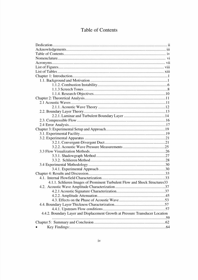
Chapter 6: Future Work ..............................................................................................65Appendices...................................................................................................................66
References..................................................................................................................127

8/6/2019 umi-umd-3786
http://slidepdf.com/reader/full/umi-umd-3786 9/146
vi
Nomenclature
a = speed of soundF(x) = amplifying (positive) or dampening (negative) effects
f = frequencyHo= constant area section duct height
K= bulk modulus of the medium
M = Mach numbern= number of measurements.Pr = reference pressure
Px = individual pressure
p = acoustic pressurep`= local pressure fluctuations
q`= oscillating energy release
R= gas constant
Rex = Reynolds numberT= temperature
t = time
U= freestream velocityu= time average velocity inside boundary layer w.r.t to y
V= uniform velocity
x = average value of the measured data, or best estimate
z = displacement along x
Greek Letters
= specific heat ratio
= boundary layer thickness
* = displacement thickness
= momentum thickness
= wavelength
µ= Mach angle or viscosity
= specific volume
= density
= standard deviation
= compressibility parameter

8/6/2019 umi-umd-3786
http://slidepdf.com/reader/full/umi-umd-3786 10/146
vii
Acronyms
AHSTF Arc-Heated Scramjet Test Facility
CAD Computer Aided Design
CHSTF Combustion-Heated Scramjet Test Facility
CHHEBD Combustion-Heated High Enthalpy Blown-Down
GASL General Applied Science Laboratory
HHT High Temperature Tunnel
ICCD Intensified Charge Coupled Device
NPT National Pipe Thread
NASP National Aero-Space Plane
PT Pressure Transducer

8/6/2019 umi-umd-3786
http://slidepdf.com/reader/full/umi-umd-3786 11/146
viii
List of Figures
Figure 1. Illustration of the first US freejet tested scramjet designed by A.Ferri……………..…...1
Figure 2. Schematic illustration of the 2-D flow dynamics inside a generic ramjet engine……….4
Figure 3. Schematic illustration of the 2-D flow dynamics inside a generic scramjet engine….…5
Figure 4. Schematic diagram of the effects of some point source traveling at supersonic speed....9
Figure 5. Schematic illustration of the first three modes of longitudinal waves inside a duct…...11
Figure 6. Pictorial view of experimental setup of supersonic flow duct in laboratory…………..12
Figure 7. Schematic illustration of the supersonic flow duct dimensional drawings layout with
all dimensions in inches.…………………………………………………………………………..20
Figure 8. Close-up view pressure transducer location inside the supersonic duct………………..21
Figure 9. 3-D isometric view of supersonic duct test setup…………………………….………..22
Figure 10. 3-D side view of supersonic duct test setup…………………….……………….…...23
Figure 11. Schematic illustration of upper component of supersonic flow duct a) side view andb) top view with all dimensions in inches…………..………………………………………….....24
Figure 12. Schematic illustration of lower component of supersonic flow duct a) side view and
b)top view……………………………………………………………………………….....…….25
Figure 13. Schematic drawing of 2-D view of convergent-divergent supersonic duct depicting
pressure transducer location relative to duct height.…………………………………….…...……25
Figure 14. Schematic drawing of shadowgraph flow visualization method…………..…............28
Figure 15. Schematic drawing of schlieren flow visualization method…………...………….…..29
Figure 16. Schematic diagram of experimental setup of supersonic flow duct in
laboratory………………………………………………………………………………..……...…32
Figure 17. Schlieren images showing the flowfield inside the nozzle, isolator for stagnation pressuresranging from 35psi to 125psi………………………………………………………………………34
Figure 18. Schlieren images showing the flowfield inside the expansion region of the duct for
stagnation pressures ranging from 35psi to 125psi……..…………………………………….…..36
Figure 19. Power Spectrum showing the magnitude of acoustic wave at a 95psi upstream stagnation
pressure with a dominant frequency of approximately 4.22kHz for a)PT2, b)PT3, c)PT4,and, d) PT5
respectively………………….…………………………………………………………………..…39

8/6/2019 umi-umd-3786
http://slidepdf.com/reader/full/umi-umd-3786 12/146
ix
Figure 20. Power Spectrum showing the magnitude of acoustic wave at a 105psi upstream
stagnation pressure with a dominant frequency of approximately 2.79kHz for a)PT2, b)PT3,
c)PT4, and ,d) PT5 respectively……………………..…….……………………………………...41
Figure 21. Power Spectrum showing the magnitude of acoustic wave at a 115psi upstream stagnation
pressure with a dominant frequency of approximately 2.78kHz for a)PT2, b)PT3, c)PT4,and ,d) PT5
respectively………………….…………………………………………….……………………..…43
Figure 22. Power Spectrum showing the magnitude of acoustic wave at a 125psi upstream stagnation
pressure with a dominant frequency of approximately 2.78kHz for a)PT2, b)PT3, c)PT4,and ,d) PT5
respectively……………………….…………………………………………………………….......44
Figure 23. Illustration of a) averaged and b) normalized dynamic pressure at each pressure
transducer location for increasing upstream stagnation pressure conditions……………….......…46
Figure 24. Illustration of a) static pressure and b) ratio of dynamic pressure to static pressure ateach PT location for increasing upstream stagnation pressure conditions………………...….....48
Figure 25. Illustration of rate of the amplitude dissipation (decibels per inch) for specificupstream stagnation pressures between a)PT2-PT3, b)PT2-PT4, and c) PT2-PT5………..…...…50
Figure 26. Illustration of rate of the amplitude dissipation (decibels per inch) for specificupstream stagnation pressures.……………..…………………………………………………..…51
Figure 27. Illustration of relative percentage of the dissipation of acoustic wave amplitude
for various stagnation pressures. .………………………………………………………………...52
Figure 28. Schematic diagram illustrating disturbance propagation in the a)downstream
direction and b) upstream direction..……………………………………………………………...52
Figure 29. Illustration of phase change along the duct for upstream stagnation pressureof a) 95psi b) 105psi………………………………………………………………….…...………54
Figure 30. Illustration of phase change along the duct for upstream stagnation pressure
of a)115 psi b) 125psi……………………………………………………………………...…..….55
Figure 31. Illustration of average phase change along the duct at each pressure transducerlocation for increasing upstream stagnation pressure conditions……………………………...….56
Figure 32. Illustration of boundary layer thickness growth along a flat plate……………......…..57
Figure 33. Illustration of a) Reynolds number and b) boundary layer thickness inside constant
area section…..…………………………..……………………………..……………………....…58
Figure 34. Illustration of turbulent displacement thickness growth inside constant area
section (isolator region)…….………..………………………………..…………………….…......59
Figure 35. Illustration of critical length as function of Reynolds number inside constant area
section (isolator region) ………………………………………………..………………………..…60
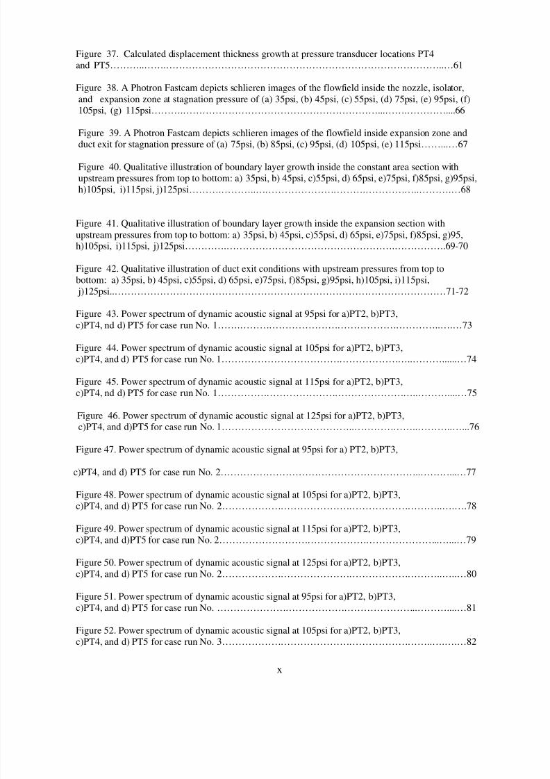
Figure 36. Calculated boundary layer thickness growth at pressure transducer locations
PT4 and PT5….…………….……………………………………………………………..…………60
8/6/2019 umi-umd-3786
http://slidepdf.com/reader/full/umi-umd-3786 13/146
x
Figure 37. Calculated displacement thickness growth at pressure transducer locations PT4
and PT5………..…….…………………………………………………………………………..…61
Figure 38. A Photron Fastcam depicts schlieren images of the flowfield inside the nozzle, isolator,
and expansion zone at stagnation pressure of (a) 35psi, (b) 45psi, (c) 55psi, (d) 75psi, (e) 95psi, (f)
105psi, (g) 115psi……….……………………………………………………...…….…………....66
Figure 39. A Photron Fastcam depicts schlieren images of the flowfield inside expansion zone andduct exit for stagnation pressure of (a) 75psi, (b) 85psi, (c) 95psi, (d) 105psi, (e) 115psi……...…67
Figure 40. Qualitative illustration of boundary layer growth inside the constant area section with
upstream pressures from top to bottom: a) 35psi, b) 45psi, c)55psi, d) 65psi, e)75psi, f)85psi, g)95psi,
h)105psi, i)115psi, j)125psi……….………..…………………………….……………..……….…68
Figure 41. Qualitative illustration of boundary layer growth inside the expansion section with
upstream pressures from top to bottom: a) 35psi, b) 45psi, c)55psi, d) 65psi, e)75psi, f)85psi, g)95,h)105psi, i)115psi, j)125psi………….…………………………………………….…………….69-70
Figure 42. Qualitative illustration of duct exit conditions with upstream pressures from top tobottom: a) 35psi, b) 45psi, c)55psi, d) 65psi, e)75psi, f)85psi, g)95psi, h)105psi, i)115psi,
j)125psi..…………………………………………………………………………………………71-72
Figure 43. Power spectrum of dynamic acoustic signal at 95psi for a)PT2, b)PT3,
c)PT4, nd d) PT5 for case run No. 1…….……………………………………………………..….…73
Figure 44. Power spectrum of dynamic acoustic signal at 105psi for a)PT2, b)PT3,
c)PT4, and d) PT5 for case run No. 1…………………………………………………..………......…74
Figure 45. Power spectrum of dynamic acoustic signal at 115psi for a)PT2, b)PT3,
c)PT4, nd d) PT5 for case run No. 1……………………………………………………..………....…75
Figure 46. Power spectrum of dynamic acoustic signal at 125psi for a)PT2, b)PT3,c)PT4, and d)PT5 for case run No. 1…………………………………..………………..………..…...76
Figure 47. Power spectrum of dynamic acoustic signal at 95psi for a) PT2, b)PT3,
c)PT4, and d) PT5 for case run No. 2……………………………………………………..………...…77
Figure 48. Power spectrum of dynamic acoustic signal at 105psi for a)PT2, b)PT3,
c)PT4, and d) PT5 for case run No. 2…………………………………………………………..….….78
Figure 49. Power spectrum of dynamic acoustic signal at 115psi for a)PT2, b)PT3,
c)PT4, and d)PT5 for case run No. 2…………………………………………………………..…...…79
Figure 50. Power spectrum of dynamic acoustic signal at 125psi for a)PT2, b)PT3,
c)PT4, and d) PT5 for case run No. 2…………………………………………………………..…..…80
Figure 51. Power spectrum of dynamic acoustic signal at 95psi for a)PT2, b)PT3,
c)PT4, and d) PT5 for case run No. ……………………………………………………..………....…81
Figure 52. Power spectrum of dynamic acoustic signal at 105psi for a)PT2, b)PT3,
c)PT4, and d) PT5 for case run No. 3………………………………………………………..….….…82
8/6/2019 umi-umd-3786
http://slidepdf.com/reader/full/umi-umd-3786 14/146
xi
Figure 53. Power spectrum of dynamic acoustic signal at 115psi for a)PT2, b)PT3,
c)PT4, and d) PT5 for case run No. 3…………………………………………………………………83
Figure 54. Power spectrum of dynamic acoustic signal at 125psi for a)PT2, b)PT3,
c)PT4, and d) PT5 for case run No. 3…………………………………………………..…..............…84
Figure 55. Power spectrum of dynamic acoustic signal at 95psi for a)PT2, b)PT3,
c)PT4, and d) PT5 for case run No. 4…………………………………………………………...….…85
Figure 56. Power spectrum of dynamic acoustic signal at 105psi for a)PT2, b)PT3,
c)PT4, and PT5 for case run No. 4…………………………………………………………...…….....86
Figure 57. Power spectrum of dynamic acoustic signal at 115psi for a)PT2, b)PT3,
c)PT4, and d) PT5 for case run No. 4……………………………………………………….…..….…87
Figure 58. Power spectrum of dynamic acoustic signal at 125psi for a)PT2, b)PT3,
c)PT4, and d) PT5 for case run No. 4……………………………………………………….…..….…88
Figure 59. Power spectrum of dynamic acoustic signal at 95psi for a)PT2, b)PT3,
c)PT4, and d) PT5 for case run No. 5…………………………………………………………...….…89
Figure 60. Power spectrum of dynamic acoustic signal at 105psi for a)PT2, b)PT3,
c)PT4, and d) PT5 for case run No. 5…………………………………………..…………………..…90
Figure 61. Power spectrum of dynamic acoustic signal at 115psi for a)PT2, b)PT3,
c)PT4, and d) PT5 for case run No. 5…………………………………………..………………..……91
Figure 62. Power spectrum of dynamic acoustic signal at 125psi for a)PT2, b)PT3,c)PT4, and d) PT5 for case run No. 5………………………..…………………………………..……92
Figure 63. Power spectrum of dynamic acoustic signal at 95psi for a)PT2, b)PT3,
c)PT4, and d) PT5 for case run No. 6……………………………………………………….…..….…93
Figure 64. Power spectrum of dynamic acoustic signal at 105psi for a)PT2, b)PT3,
c)PT4, and d) PT5 for case run No. 6…………………………………………………………......…..94
Figure 65. Power spectrum of dynamic acoustic signal at 115psi for a)PT2, b)PT3,
c)PT4, and d) PT5 for case run No. ……………………………………………………………..……95
Figure 66. Power spectrum of dynamic acoustic signal at 125psi for a)PT2, b)PT3,
c)PT4, and d) PT5 for case run No. ……………………………………………………………....…..96
Figure 67. Power spectrum of dynamic acoustic signal at 95psi for a)PT2, b)PT3,
c)PT4, and d) PT5 for case run No.7…………………………………………………..………..….…97
Figure 68. Power spectrum of dynamic acoustic signal at 105psi for a)PT2, b)PT3,
c)PT4, and d) PT5 for case run No. 7…………………………………………………………..…..…98
Figure 69. Power spectrum of dynamic acoustic signal at 115psi for a)PT2, b)PT3,
c)PT4, and d) PT5 for case run No. 7…………………………………………………………..…..…99
Figure 70. Power spectrum of dynamic acoustic signal at 125psi for a)PT2, b)PT3,
c)PT4, and d) PT5 for case run No. 7…………………………………………………………..……100

8/6/2019 umi-umd-3786
http://slidepdf.com/reader/full/umi-umd-3786 15/146
xii
Figure 71. Power spectrum of dynamic acoustic signal at 95psi for a)PT2, b)PT3,
c)PT4, and d) PT5 for case run No. 8…………………………………………………………..……101
Figure 72. Power spectrum of dynamic acoustic signal at 105psi for a)PT2, b)PT3,
c)PT4, and d) PT5 for case run No. 8…………………………………………………………..……102
Figure 73. Power spectrum of dynamic acoustic signal at 115psi for a)PT2, b)PT3,
c)PT4, and d) PT5 for case run No. 8…………………………………………………………..……103
Figure 74. Power spectrum of dynamic acoustic signal at 125psi for a)PT2, b)PT3,
c)PT4, and d) PT5 for case run No. 8…………………………………………………………..……104
Figure 75. Power spectrum of dynamic acoustic signal at 95psi for a)PT2, b)PT3,
c)PT4, and d) PT5 for case run No. 9…………………………………………………………..……105
Figure 76. Power spectrum of dynamic acoustic signal at 105psi for a)PT2, b)PT3,
c)PT4, and d) PT5 for case run No. 9…………………………………………………………..……106
Figure 77. Power spectrum of dynamic acoustic signal at 115psi for a)PT2, b)PT3,
c)PT4, and d) PT5 for case run No. 9…………………………………………………………..……107
Figure 78. Power spectrum of dynamic acoustic signal at 125psi for a)PT2, b)PT3,
c)PT4, and d) PT5 for case run No. 9…………………………………………………………..……108
Figure 79. Power spectrum of dynamic acoustic signal at 95psi for a)PT2, b)PT3,
c)PT4, and d) PT5 for case run No. 10…………………………………………………………....…109
Figure 80. Power spectrum of dynamic acoustic signal at 105psi for a)PT2, b)PT3,c)PT4, and d) PT5 for case run No. 10…………………………………………………………....…110
Figure 81. Power spectrum of dynamic acoustic signal at 115psi for a)PT2, b)PT3,
c)PT4, and d) PT5 for case run No. 10………………………………………………………………111
Figure 82. Power spectrum of dynamic acoustic signal at 125psi for a)PT2, b)PT3,
c)PT4, and d) PT5 for case run No. 10………………………………………………………………112
Figure 83. Power spectrum analysis at individual pressure transducers for stagnation
pressure 95psi…………………………………………………………………….……………….….113
Figure 84. Power spectrum analysis at individual pressure transducers for stagnation
pressure 105psi…………………………………………………………………………………….…114
Figure 85. Power spectrum analysis at individual pressure transducers for stagnation
pressure 115psi…………………………………………………………………………………….…114
Figure 86. Power spectrum analysis at individual pressure transducers for stagnation
pressure 125psi………………………………………………………………………………………..114

8/6/2019 umi-umd-3786
http://slidepdf.com/reader/full/umi-umd-3786 16/146
xiii
List of Tables
Table 1. Error analysis values for ratio of dynamic pressure to static pressure……………...…115
Table 2. Phase analysis w.r.t upstream stagnation pressure of 95psi…………..…………….…116
Table 3. Phase analysis w.r.t upstream stagnation pressure of 105psi…………..………………117
Table 4. Phase analysis w.r.t upstream stagnation pressure of 115psi…….………………….…117
Table 5. Phase analysis w.r.t upstream stagnation pressure of 125psi…………..………………117
Table 6. Static pressure at each pressure transducer location w.r.t upstream stagnation
pressure of 80psig…………………….……………………………………………………..118-119
Table 7. Static pressure at each pressure transducer location w.r.t upstream stagnation
pressure of 90psig……………………………………………………………………………120-121
Table 8. Static pressure at each pressure transducer location w.r.t upstream stagnation
pressure of 100psig…………………………………………………………………………..122-123
Table 9. Static pressure at each pressure transducer location w.r.t upstream stagnation
pressure of 110psig………………………………………………………………………..…124-125
Table 10. Calculated values fro amplitude attenuation in decibels…………………….………...126
Table 11. Calculated values for percent dissipation……………..…………………………….....126
8/6/2019 umi-umd-3786
http://slidepdf.com/reader/full/umi-umd-3786 17/146
1
Chapter 1: Introduction
1.1. Background and Motivation
As the world of aviation moves closer and closer towards the reality of hypersonic flight, the engines that are
projected to power these vehicles for this lofty endeavor are predicted to be supersonic combustion ramjets,
otherwise known as scramjets. Before the start of developmental research on scramjet engines in the 1960’s,
ramjet engine technology has been the focus of study for high-speed air breathing propulsion since the 1940’s in
the United States.1
During this time, other nations were also conducting research on hypersonic vehicle
propulsion systems. Mestre and Viaud (1964) of France performed several scramjet engine experiments by
burning kerosene/air in a constant area supersonic duct.2 Scramjet research and development in Russia, or the
former Soviet Union, was established primarily by Prof. E.S. Shchetinkov at the Central Aerohydrodynamic
Institute.3 Building upon the successes in the advancement of ramjet engines, Shchetinkov and other scientist at
the Central Institute of Aviation Motors continued to examine some of the fundamental issues of scramjet
engines. Such problems as fuel-air mixing and burning in a supersonic flowfield over some practical length
became central to their research.3 The earliest research and development of scramjet engines in Japan was
carried out during the 1970’s. Experiments were primarily conducted in the universities, which focused on the
ignition mechanism for a diffusion flame in a supersonic flowfield.4
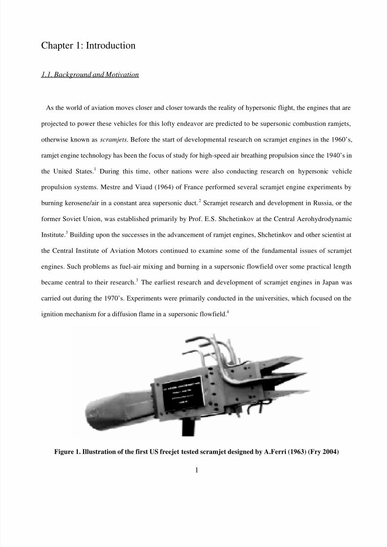
Figure 1. Illustration of the first US freejet tested scramjet designed by A.Ferri (1963) (Fry 2004)

8/6/2019 umi-umd-3786
http://slidepdf.com/reader/full/umi-umd-3786 18/146
2
The propulsion cycle of scramjet engines allow the vehicle to perform over a broader flight Mach number
envelope in comparison to vehicles flying with conventional airbreathing engines. Efficient operation for typical
liquid fueled scramjets occurs at flight Mach number range6
of M= 3 to 10. In comparison to liquid fueled,
gaseous fuel scramjets can be efficiently operated up to orbital speeds. One of the critical constraints for liquid
fuel type scramjets is the factor of energy consumption during ionization and dissociation. Academic
institutions and other research entities have found a litany of fundamental problems that need to be addressed
and if possible completely solved before the realization of efficiently operating scramjet and ramjet engines
become successfully integrated in future aircraft. Some of the critical problems facing the successful
development of these engines include understanding complex flowpath, efficient fuel injection, mixing and
combustion, as well as suppressing combustion instability. With the captured air inside the inlet region, it
becomes critical to ascertain the complex flowfield irrespective of the flow channel’s geometric configuration6.
Specifically, according to Waltrup6, a thorough comprehension about the compressible flowfield (externally and
internally) coupled with shockwave dynamics is needed.
Another critical area of interest is fuel injection. Problems associated with this area can be broken down into
two types: wall (normal) injection and axial (transverse) injection.6 In terms of wall fuel injection into the
flowfield, a detailed knowledge of how the fuel breaks down to the smallest possible sizes (atomization),
disintegrates, and imbeds into the flowfield becomes necessary.6 According to Waltrup6, the axial fuel injection
issues are focused around the dynamics of free shear layer growth. In addition, fuel ignition characteristics with
respect to “thermochemical properties” are particular interests that require major research effort. Within the
combustor, the focus is on optimizing the amount of heat release and pressure losses, which are the two driving
factors of its development.6
While attempting to maximize the thrust output of the engine, it becomes critical to
keep in mind the optimum combustor length in order to accomplish this objective. It is equally vital to grapple
with the issue of how the fuel-air entrainment (mixing process) over the specified design combustor length can
be carried out efficiently.6 Therefore, mixing and burning with timescales on the order of milliseconds are
problems that have elicited the attentive efforts of many.
8/6/2019 umi-umd-3786
http://slidepdf.com/reader/full/umi-umd-3786 19/146
3
According to Ma et al.7, there seems to be a general consensus that acoustic wave upstream propagation inside a
supersonic flowfield is not possible. The thought is that pressure oscillations inside the combustor will not
interact with the flame front to create a closed-loop feedback, which is essential for the prolonged combustion
instability.7 This idea would be correct if the subsonic boundary layer region of the flowfield inside the duct
was neglected.
Ma et al.7 proclaimed that a different point of view was needed and that these combustion oscillations in the
form of acoustic waves can propagate upstream via any subsonic portion of the flowfield i.e. boundary layer or
recirculation regions. This is, in essence, the primary motivating reason behind this research effort.
1.1.1. Scramjet and Ramjet Historical Evolution
Ramjet engines, which are subsonic combustion engines, were the main focus of air-breathing propulsion
R&D between the 1940’s and 1960’s in the United States. Research institutions involved in ground testing and
flight testing were NASA Langley (Wallops Station), Navy (China Lake), and U.S. Air Force (Marquardt).8 In
the early 1960’s, the aerospace research community realized that supersonic combustion ramjets (scramjets)
were needed in order to accomplish the goal of achieving hypersonic flight.8 By the middle of the 1960’s, free-
jet engine testing programs began to take hold. Testing was conducted mostly in propulsion test facilities that
accommodated the high-energy exhaust from the nozzle. At the General Applied Science Laboratory (GASL),
the Combustion-Heated High Enthalpy Blown-Down (CHHEBD) Tunnel conducted the first free-jet tests of the
first known scramjet engine in 1963, see Figure8
1. This scramjet engine was a fixed geometry model, which
was designed by Dr. A. Ferri.8 After a decade of “non-airframe integrated” engine testing, the push towards
integrating the engine on an airframe became the primary objective. Testing facilities dedicated to sub-scale
engine propulsion were established at NASA Langley. From the mid 1970’s to mid 1980’s, the Arc-Heated
Scramjet Test Facility (AHSTF) and the Combustion-Heated Scramjet Test Facility (CHSTF) were mainly used
for testing and development of these sub-scale engines. For large-scale engine testing, such as the National
AeroSpace Plane (NASP), the Langley High-Temperature Tunnel (HHT) was used in the early 1990’s. The

8/6/2019 umi-umd-3786
http://slidepdf.com/reader/full/umi-umd-3786 20/146
4
Advanced Research for Transportation Technology program directed by NASA Marshall continues to push the
envelope in sub-scale engine research today.
The cooperative efforts by NASA Dryden and Langley oversee the execution of the Hyper-X Project. The
steady progress in scramjet engine research can be attributed to the great strides made in the advanced
development of Computational Fluid Dynamics as well as dedicated and in-depth research for scramjet inlet and
combustor development.8
1.1.1.1. Scramjet and Ramjet Engines Flow Dynamics
Figure 2. Schematic illustration of the 2-D flow dynamics inside a generic ramjet
engine
In describing the overall flow dynamics through a ramjet engine, a schematic diagram, see Figure 2,
will be used to illustrate the critical portions of the engine. Starting from left to right with the freestream
conditions, the airflow enters the diffuser, which is mainly used to decelerate the flow. At the tip of the
vehicle’s forebody an oblique shock is used to compress the air, which is the beginning of the flow
deceleration process. Deceleration continues through a series of normal shocks, also known as a shock
train, and then travels through the divergent portion of the duct just before the entrance of the subsonic
burner. Inside the burner, the subsonic air stream mixes and burns with the injected fuel. 9 The combustion
products at high pressures are then accelerated to supersonic speed through the convergent-divergent
portion of the exhaust nozzle.
Nozzle
Fuel Injectors
Subsonic BurnerDiffuser
Shock Trains
Diffuser
Oblique Shock
Wave
Free Stream
Flow
Supersonic
Exhaust Flow
Engine Cowl
Flame Holders
M<1
M >1
M >1

8/6/2019 umi-umd-3786
http://slidepdf.com/reader/full/umi-umd-3786 21/146
5
With greater momentum at the exit plane of the engine than at the inlet plane, the ramjet engine is able to
exert thrust on the vehicle in order to propel it in the forward acting direction.9
Figure 3. Schematic illustration of the 2-D flow dynamics inside a generic scramjet
engine
At the limiting case for flight region of Mach 6, the ramjet engine becomes impractical. The critical reason for
this is due in part to what happens to the energy during the deceleration process. The diminishing kinetic energy
is transferred into internal energy of the flowfield9. Consequently, one can observe the significant increase in
temperature, pressure, and density at the burner entrance. These conditions could escalate even more with
increasing Mach number. With such disadvantageous conditions, numerous effects such as large heat transfer
rates at the wall, diminishing combustor integrity, as well as engine performance losses may ensue. To resolve
some of these detrimental effects, the flowfield entering the combustor should be supersonic instead of subsonic
as seen in the ramjet engine. The key point in doing this is to reduce the amount of loss in kinetic energy being
transferred into internal energy and hence less rate of pressure, temperature, and density with increasing Mach
number.
The generic operation of a scramjet engine and its major components can be described using Figure93.
Oblique shock waves from the forebody and diffuser compress the supersonic freestream flow to the design
burner entrance supersonic Mach number.
Diffuser Supersonic Burner Nozzle
Engine Cowl
Fuel Injectors
Forebody
Oblique Shock
Wave
Free Stream
FlowSupersonic
Exhaust FlowM >1
M >1
M >1

8/6/2019 umi-umd-3786
http://slidepdf.com/reader/full/umi-umd-3786 22/146
6
Inside the supersonic combustor, fuel is then injected at the optimum location to allow for complete mixing and
burning in a short period of time (short combustor length less structural mass).9 This is arguably one of the most
critical aspects of a successful development of scramjet engines. This area of research has been and is currently
being pursued at the Advance Propulsion Research Laboratory (University of Maryland, College Park) as well
as many other institutions and laboratories across the nation and the world. Finally, the divergent nozzle
provides the needed acceleration for the high-speed combustion products.
1.1.2. Combustion Instability
As mentioned before, a greater understanding of the fundamental physical phenomena that exists inside the
combustor of these high-speed vehicles (i.e. hypersonic vehicles) is essential to successful development and
implementation of engines such as scramjets and ramjets. Application requirements of modern propulsion
system are the primary driving force behind which of these parameters, for example performance, NOx output,
fuel efficiency, and maintenance cost, will take a higher priority level for optimization.10
Given the increasing
demand on contemporary power plants, it has become a top priority in recent years to address some of these
phenomena. A critical phenomenon that is of interest is the combustion instability that is recognized in
propulsion systems.
11
In general, the combustion instabilities that are observed in propulsion systems are large
amplitude pressure oscillations that are intensifying sporadically out of the noise that occur during the
combustion process.11
According to Roy10
, one may describe these combustion instabilities as a very dynamic
and complex feedback process that occur when these oscillations of single or multiple acoustic modes are
driven by the perturbation during combustion. Historically, the first studies conducted on combustion instability
phenomenon were focused on liquid rocket engines in countries such as Germany, Russia, and the United States
during WWII
11
.
Currently, combustion instabilities are not only being addressed in rockets but also in liquid fueled air-
breathing propulsion systems (ramjets and, scramjets, and gas turbines) as well in burners.12 In essence, these
combustion instabilities are produced by the amplification of the disturbances in the flow by the coupled effects
of the heat release during combustion and the generated acoustic energy.13
The self-sustainability of the
instabilities is driven by the continuous reinforcement of the acoustic energy.

8/6/2019 umi-umd-3786
http://slidepdf.com/reader/full/umi-umd-3786 23/146
7
The performance and structural integrity of the propulsion system will be compromised with the detrimentally
increasing effects of the expected thermal and mechanical loads from these combustion instabilities.13 Lord
Rayleigh, who addressed this issue in 1878, stated that the acoustic disturbances receive a continuous influx of
energy if the energy release during the combustion process is “in phase” with the transient pressure conditions.
This concept known as Rayleigh’s Criterion can be expressed mathematically with the following formula,
according to Roy10
.
( ) ( ) =
T
dt t x pt xqT
xF ,,1
)( (1)
where T= period of investigation
F(x)= amplifying (positive) or dampening (negative) effects
q`(x,t)= oscillating energy release
p`(x,t)= local pressure fluctuations
The current consensus is that, for theoretical and empirical pursuits, the understanding and implementation
of the formulation (1) will bolster the capability of attenuating the disturbances in the combustor, but doesn’t
necessarily improve the total performance of the engine.10 A thorough look at the mixing enhancement methods
as well as various control mechanism for pressure fluctuations may be warranted. For a more in-depth
understanding of the intricate details that are involved with these instabilities, a list of relatively current
numerical and experimental research work involving the flowfield, vortex structures, small scale turbulent
structures, and thermoacoustic oscillations is documented by Roy.10 The promising research work in
combustion control, which include active as well as passive control has been at the forefront of combustion
instability research.14-21
One may describe active combustion control as a manipulative technique that utilizes
sensor control mechanisms to suppress the amplified oscillations in the combustor. While on the other hand, the
means of passive control which is more limited in it implementation, where expenses can accrue rapidly due to
constant modification to distinct systems.14 The mode of oscillations that are typically observed in combustors
8/6/2019 umi-umd-3786
http://slidepdf.com/reader/full/umi-umd-3786 24/146
8
falls under the categories of low and high frequency oscillations. In general, low frequencies are associated with
longitudinal modes while high frequencies are associated with transverse modes, which produce the very
noticeable “screeching” sound.13
1.1.3 Screech Tones
In order to simulate the large pressure oscillations that are associated with these combustion instabilities, an
acoustic phenomena known as screech tones have been implemented as a passive excitation mechanism during
this experiment. Screech tones were first studied by A. Powell in the early 1950’s at the University of
Southampton in England.22 According to Raman, Powell used the schlieren flow visualization technique on a
small-scale jet when this phenomenon was observed. He studied both two dimensional and circular jets and
proposed a “phased array model” that brought forth the formulae for the screech frequency and directivity.22
Powell described these screech tones as “embryonic disturbances” that are produced at the nozzle lip. As they
propagated downstream, these vortex structures grow and in the process combine with the “shock cells” in order
to generate sound. The generated sound then propagates back upstream to nozzle tip where the resonant loop is
established.22 In this experiment, it was observed that the overexpansion of the supersonic jet at the exit plane of
the duct oscillates periodically which produced these very audible screech tones. The supersonic flow was
discharged into the tube from the nozzle lip of both the top and bottom components of the supersonic duct.
Shear layer growth and shock interactions occur such that a passive acoustic excitation is created. This
oscillation can propagate upstream through the fluid medium via the boundary layer. How far upstream and
how much dissipation has occurred are the fundamental focuses of this research.
A previous study that dealt with sound waves passing through a turbulent boundary layer examined
the problem on two fronts experimentally and theoretically.23
Experimentally, the test was modeled as
boundary layer flow over a flat plate where the attenuation of sound was examined. With Mach
numbers reaching up to as high as 0.8, the authors used a flat plate that was attached to one side of this
high speed jet.23 The authors found significant losses of sound transmission for high frequency signal
in the forward direction. Theoretically, the authors developed a model of the sound propagation that

8/6/2019 umi-umd-3786
http://slidepdf.com/reader/full/umi-umd-3786 25/146
9
took into account refraction due to velocity and various density levels of the turbulent boundary
layer.23 They discovered that the frequency of the sound wave, the measurement angle, and the Mach
number of the jet had a strong effect on eddy viscosity and how it relates to acoustic transmission
losses. The investigation carried out during this experiment rest on the fundamental basis that
upstream propagation of acoustic waves will occur via the subsonic boundary layer and not the
supersonic core flow.
This concept that disturbances of any types will not propagate upstream through the purely supersonic flow is a
fundamental physical property of supersonic flow.24 It is well know that a body in a supersonic stream will
create a Mach cone with concentric circles that separate regions called zone of action and zone of silence,
25
see
Figure 4.
Figure 4. Schematic diagram of the effects of some point source traveling at supersonic speed
The schematic diagram in Figure 4 illustrates a critical concept known as the “rule of forbidden signals”.
26
This
fundamental principle in supersonic flow simple states that a body moving a supersonic speed will produce
pressure perturbations that will fall behind the body itself. The creation of a wave front in the form of Mach
cone with the moving body at the vertex point.26 It is assumed that the body travels with uniform velocity, V;
the distance traveled is therefore “Vt”. The angle, from the central point, of the cone is called the Mach angle,
µ, which is defined as {µ= sin-1(1/M)}, where M= V/a. This Mach number (M) is defined as the local velocity
3 at
Mach Cone
Zone of Action
Zone of Silence
Zone of Silence
µ
Mach Angle
1Vt
3Vt
2Vt

8/6/2019 umi-umd-3786
http://slidepdf.com/reader/full/umi-umd-3786 26/146
10
of the moving body divided by the local speed of sound ”a”. The zone of action is the region that is located
within the Mach cone, where disturbances propagate downstream of the moving point source. Beyond the
boundaries of the Mach cone, the zone of silence stretches upstream of the moving body such that no detection
of the signal is permitted in this zone.25
This concept essentially forms the assertion of this research, where it is
assumed that the signal propagation will not be felt inside the supersonic stream but only in the subsonic regions
of the flow, where the disturbances propagate in all directions.
1.1.4. Research Objectives
In order to give this research effort a well-defined direction, a few realistic objectives are desired to
accomplish this mission. First, one would like to examine whether or not the downstream disturbances will
propagate upstream through the supersonic duct. To answer the question of how far the perturbations could
propagate upstream, one would examine the dissipation effects of the acoustic wave amplitude (intensity) as it
propagates upstream through the boundary layer of a supersonic flow duct. Finally, one then would characterize
the dampening mechanism and investigate whether or not a control mechanism can be implemented in this
experiment. A characterization of the amplitude with respect to the horizontal distance (x) was carried out.

8/6/2019 umi-umd-3786
http://slidepdf.com/reader/full/umi-umd-3786 27/146
11
Chapter 2: Theoretical Analysis
2.1 Acoustic Waves
L f
21
=
L21 =
L f
=
2
L=2
L f
2
33
=
L3
23 =
Figure 5. Schematic illustration of the first three modes of longitudinal waves inside a duct
Waves, in general, come in various types such as water waves that move across the ocean, distortional waves
that oscillate within vibrating bodies. They also include sound waves, which transmit or carry tones and noises
through the air and electromagnetic waves that transmit light, x-ray, infrared, etc… Wave propagation can be
viewed as motion of a disturbance through some medium.27 A typical example of this is the motion of some
impulse of disturbance along a string or stretched out horizontally or vertically. Most waves can be classified as
either longitudinal or transverse waves.
Node Antinode
L
fundamental mode
(1st
harmonic)
2nd harmonic
3rd harmonic

8/6/2019 umi-umd-3786
http://slidepdf.com/reader/full/umi-umd-3786 28/146
12
Longitudinal waves are, in essence, waves in which the vibrating motion of the particles moving forward and
backward parallel to the direction of the wave propagation. On the other hand, transverse waves are generally
described as waves in which the particles vibrate perpendicular to the direction the wave motion.27
One may
think of acoustic waves as mechanical waves with physical attributes. As a result, the medium of wave
propagation must have inertia and elasticity for successful transmission.27
Waves also transmit energy along the
direction of propagation. The energy maybe transformed in various waves. In the case of a wave traveling from
one medium to the next, the waves tend to distribute their energy proportionally. This distribution process may
occur as a reflection, transmission, and absorption. This idea is analogous to light waves striking a glass, where
part of it is reflected, most transmitted through the glass, while still a small potion is absorb by the glass. When
energy of wave is completely absorb by its medium this absorbed energy is usually converted to heat.27
2.1.1. Acoustic Wave Theory
It is well known that sound wave in air propagates longitudinally, where the oscillations takes place in the same
direction of the wave motion.28
This type of wave motion can be describe mathematically as the following:
Assume one dimensional traveling wave,
2
2
22
2 1
t
z
c x
z
=
(2)
where,
z = displacement along x
c = velocity of sound
t = time
Solutions to equation (2) can describe the longitudinal motion of waves in pipes and ducts with specified
boundary conditions. The acoustic pressure is related to “z” in terms of the following, where K= bulk
modulus of the medium,28

8/6/2019 umi-umd-3786
http://slidepdf.com/reader/full/umi-umd-3786 29/146
13
zK p
= (3)
Emphasis during this research wasn’t placed upon the rigorous determination of the exact solution to equation
(2) due to the necessity of more in-depth understanding of the complex flow field. This could be pursued as
future research interests, maybe examining the two and three-dimensional solutions.
For this research work, a first cut approximation of the acoustic mode of the supersonic duct was obtained by
using the model in Figure 5. This is a double open channel depicting the general shape of the first
(fundamental), second, and third harmonics. The oscillating air column produces nodal and anti-nodal points,
see Figure 5. A displacement anti-node is observed at each end where the maximum displacement occurs due to
the freely moving air. While, the minimal displacement occurs at the nodal points.29 The frequency and
wavelength can be estimated by using the formulas given in Figure 5. Assuming a constant area channel with a
length of 12 inches (305mm), the fundamental frequency (first harmonic) was calculated as being
approximately 567 Hz. The higher harmonics were estimated as 1134Hz and 1700Hz, 2nd
and 3rd
harmonics
respectively. These values were based on constant velocity of sound, with constant temperature (298K). This
analysis was pertinent in order to gauge what role the supersonic duct’s inherent acoustic modes would play in
this experiment. Based on the dominant frequency of the passive acoustic mechanism, there is little probability
that resonance would occur between the screech tones and natural frequency of the supersonic duct.
2.2. Boundary Layer Theory
The concept of a boundary layer development along a surface was first presented by Ludwig Prandtl in
Heidelberg, Germany (1904).30 The significance of this concept is the fact that it allowed engineers and scientist
to execute viscous flow analysis. The practical application for such a concept was used to generate drag and
flow separation theoretical data for aerodynamic principles.30 The boundary layer equations, which are
obtained from the full Navier–Stokes Equations were derived based on the assumption that boundary layer is
adjacent to some aerodynamic body. Solving these boundary layer equations produced solutions for heat
8/6/2019 umi-umd-3786
http://slidepdf.com/reader/full/umi-umd-3786 30/146
14
transfer and distributions of shear stress across the surface.30
The boundary layer is essentially the region of
flow that is adjacent to the surface is considerably thin in comparison to the core flowfield.29 In ideal fluid
analysis, the viscous terms in the momentum equation as well as the heat conduction for energy equation in the
governing equations of fluid dynamics are usually ignored in order to allow for rapid calculations this
assumption leads to the Euler equations.31 One may think this ideal or inviscid case as a flow in which the
infinitely approaching Reynolds number becomes a dominant constraint.
In this experiment the boundary layer theory is focused on the assumption of flow over a flat plate. A few
critical assumptions are that the boundary layer is much thinner than the parameterize length of the flat plate
and the non-slip condition at the surface. Also, the Reynolds number is assumed very large and its inverse is on
the same order of magnitude as the boundary layer thickness squared. 32 Another critical assumption is that at a
given point x along the flat plate the pressure gradient perpendicular to the surface is negligible as follows:
0=
y
p(4)
In essence, pressure can be assumed constant along the vertical axis from the surface to the outer edge of the
boundary layer at the lower limit of the main core flow.32 The growth of the boundary layer reduces the cross-
sectional area for the core or central flowfield in a channel flow. Hence, for supersonic wind tunnel, the flow
will increase for a subsonic flow field and decreases for supersonic according to the Area-Mach number
relation.31
2.2.1. Laminar and Turbulent Boundary Layer
Fundamental solutions to the boundary layer equations are based upon whether the flow is laminar or turbulent.
Typically, laminar flow can be considered as smooth fluid motion where the mass transport between the
adjacent fluid layers is negligible.33
In essence the fluid elements seem to steadily glide over each other instead
of exhibiting some random motion. In contrast to laminar flow, turbulent flow, as the name suggest, is more
unpredictable and erratic motion of the fluid particles. The oscillation of the velocity occurs along the normal
and along the direction of the average core flow.33
According to Anderson,30
the increased energy of the

8/6/2019 umi-umd-3786
http://slidepdf.com/reader/full/umi-umd-3786 31/146
15
turbulent structures translate into larger velocity profile for turbulent boundary layers than in the case of laminar
boundary layers. The less likely hood of flow separation for turbulent boundary layers than laminar boundary
layers can also attribute to the fact of increasing energy of the turbulent flow. The approximated analysis for the
boundary layer thickness () and displacement thickness (*) was based on the turbulent boundary layer
analysis. Kreider34 provided an approximated solution with use of polynomial data fit of the velocity profile,
which is known as the power law to the one-seventh scale, given as follows:
7 / 1
=
y
U
u(5)
where u= time average velocity inside boundary layer w.r.t to y
U= freestream velocity
= boundary layer thickness
The boundary layer thickness in this analysis is based on the assumption that the time average velocity (u) is
99% of the velocity at its outer edge.30
The boundary layer thickness, displacement thickness, and Reynolds
number were approximated with the following equations,
5 / 1Re
368.0
x
turb
x= (6)
5 / 1
*
Re
046.0
x
turb
x= (7)
µ
Ux x =Re (8)

8/6/2019 umi-umd-3786
http://slidepdf.com/reader/full/umi-umd-3786 32/146
16
2.3. Compressible Flow
Compressible flow is usually defined as “variable density flow”.24
In comparison to incompressible flow,
where the density remains relatively constant, compressible flow is mainly considered as any flow regime
where the density changes with time. Let’s examine the compressibility parameters of a fluid, where the
compressibility is defined as:
dp
d
1= ( 9)
where is the compressibility parameter, is the specific volume , while p is the pressure. The physical
meaning behind the compressibility can be observed as the fractional change in volume of the fluid element per
unit change in pressure.24
To obtain an even more accurate definition of compressibility, one would take into
account the ratio of partial change in specific volume and pressure with respect to temperature or isentropic
changes. In terms of change in density, where density () is defined as the inverse of the specific
volume,
1
= . Given the definition of density and equation 9, the change in density with respect to the
change in pressure and the compressibility parameter is as follows:24
dpd = (10)
It can be shown that speed of sound, “a”, defined as the square root of the partial change in pressure and density
through an isentropic process.24
s
pa
=
(11)
Equation 11 is considered the general relation for the speed of in a gas. For a calorically perfect gas and in terms
of specific heat ratio , gas constant R, and the temperature T, an alternate definition can be obtained for the
speed of sound, where
RT a = (12)

8/6/2019 umi-umd-3786
http://slidepdf.com/reader/full/umi-umd-3786 33/146
17
2.4 Error Analysis
All experimentalists understand that whenever an experiment is conducted it is subjugated to errors and
uncertainties. Therefore it becomes critical to quantify the errors associated with experimental data collection.
In essence one looks at the accuracy, precision, and sensitivity to describe the quality of the experimental data.34
Accuracy is generally defined as a measure of the relative proximity of the measured data to the true value.
Basically how close the collected data comes to the true value. Hence, the closer the measured value to the true
value the greater the accuracy. In terms of precision, it is usually describe as a measure of repeatability. How
repeatable are one’s measurements of the same test multiple times sequentially is answered by the level of
preciseness of the data. In addressing the sensitivity, it is often considered as being the relative measured affect
produced by a change in the value of the quantity that was measured. Basically, how much some parameter
changes as a result of the change in the measured quantity. A quantitative measure of preciseness can be carried
out by statistical analysis. The general idea is that as you increase the number of times a measurement is taken
the more precise the measurement. In order to address this issue, statisticians develop what is known as the
“Student’s t Table”, which relates the standard deviation of a certain set of measurements of the same measured
parameter.24
Mathematically the standard deviation is given by
( )
1
2
n
x x (13)
where x = measured data
x = average value of the measured data, or best estimate
n= number of measurements.
The standard deviation tells how much the data is distorted around the true value. In this experiment the error
analysis focuses mainly on the standard deviation of the measured quantity. The standard deviation is used in
calculating the product or quotient of a desired value. For example, an investigation of the ratio of the dynamic
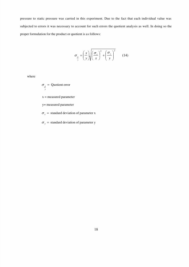
8/6/2019 umi-umd-3786
http://slidepdf.com/reader/full/umi-umd-3786 34/146
18
pressure to static pressure was carried in this experiment. Due to the fact that each individual value was
subjected to errors it was necessary to account for such errors the quotient analysis as well. In doing so the
proper formulation for the product or quotient is as follows:
22
+
=
y x y
x y x
y
x
(14)
where
=
y
x Quotient error
x = measured parameter
y= measured parameter
= x standard deviation of parameter x
= y standard deviation of parameter y

8/6/2019 umi-umd-3786
http://slidepdf.com/reader/full/umi-umd-3786 35/146
19
Chapter 3: Experimental Setup and Approach
3.1. Experimental Facility
In order to investigate this problem of acoustic wave propagation through a supersonic flow duct, a two-
dimensional channel that simulates scramjet a scramjet engine was designed and manufactured to examine this
critical issue. As mentioned before, this experiment was a non-reacting (cold flow) investigation that mainly
focused on the characterization of acoustic wave transmission inside the supersonic duct. This experiment was
conducted using a Mach 2 convergent-divergent nozzle. Through a two inch NPT circular steel pipe, high
pressure air was delivered from a stationary, single-stage, oil-injected screw type compressor into the
supersonic duct inlet with a 0.5-in2
cross-sectional area. The Atlas Copco Compressor is capable delivering a
maximum volumetric flow rate of air at 358 ft3 /min for pressures up to 150psi. A settling tank, which is
connected to the compressor, provides a means of removing particle deposits and oil residue. Branching directly
from the settling tank is a compressor line to a dryer, which basically eliminates the condensate by reducing the
temperature to freezing levels. Before air is delivered to the inlet of the test rig, it was ultimately passed through
a gas/air filter. A quarter ton valve upstream of duct inlet provides the mechanical means of turning on and off
the flow of air, which subsequently goes through a heavy duty Wilkerson screw type regulator, which is rated
for a pressure range of 0 to 180psi.
Figure 6. Pictorial view of experimental setup of supersonic flow duct in laboratory
Exhaust Duct
Kistler
Power/Signal
Conditioner
Supersonic Flow ApparatusAir Flow
Kistler Dynamic PT Location
Exhaust TubeAcoustic Source PT
Static Setra Pressure
Transaducers
Setra Pressure
Transaducers DatumsLabview DAQ Board

8/6/2019 umi-umd-3786
http://slidepdf.com/reader/full/umi-umd-3786 36/146
20
The airflow is then transitioned from a circular pipe to a rectangular cross-section area with an O-ring seal
providing airtight sealing on the transition block, see Figure 6 for a pictorial view of experimental set up. From
the inlet region of the supersonic duct in Figure 5, airflow is then accelerated to Mach 1 at the throat of the
convergent-divergent (c-d) nozzle. At approximately 78.74-inches (2m) upstream from the throat area of the
nozzle, a 120 psig rated Setra Model 206 pressure transducer was used to measure the stagnation pressure at the
choked flow regulator. The airflow is expanded from the sharp-cornered throat to a Mach 2 flow at the nozzle
exit area with use of a nozzle profile, which was designed from the method of characteristics calculation. From
the nozzle exit in the duct, the airflow travels through a constant area section of 0.213-in2 (137.419 mm2), which
can be viewed as an isolator region. Flow is then expanded through a diverging section with an angle of 3° from
the horizontal. The reason for this was mainly to avoid the Fanno effect, where unwanted choking due to
friction becomes prominent. Once the upstream flow conditions are established, the static pressure and dynamic
pressure measurement can be obtained separately via the Setra Model 206 pressure transducers and the Kistler
high-frequency response PT. The static pressure measurements were displayed using Setra’s dual channel
Datum 2000, while the dynamic pressure signals were transmitted to the Kistler Power and Conditioning Units.
A detailed pictorial illustration of the experimental setup with the data acquisition is depicted in Figure 6. A
National Instrument DAQ board served as the interface between the raw signal and Labview, which is
essentially a real time based virtual laboratory software.
Figure 7. Schematic illustration of the supersonic flow duct dimensional drawings layout
with all dimensions in inches.
Flow Transition
Section
Air Supply Pipe
Supersonic DuctExhaust Tube
Air Flow

8/6/2019 umi-umd-3786
http://slidepdf.com/reader/full/umi-umd-3786 37/146
21
A 2-D view of the assembled supersonic duct with dimensions at critical areas such as the throat area, 0.126-in2
(81.29 mm2) of the c-d nozzle, the constant area section, and expansion region are shown in Figure 7.
3.2. Experimental Apparatus
3.2.1. Convergent-Divergent Duct
The top and bottom components of the duct were inserted and fixed between two one-inch (25.4mm) thick
steel metal plates. The plates were designed with flow visualization area dimensions of 1.2 inches (30.48mm)
high and 11.8-inches (299.72mm) long that is sealed on both sides with two (12-in x 2-in x 0.5-in) polished
quartz glass. Below the test section (isolator and expansion regions), as seen in Figure 8, a bank of the Kistler
high frequency response pressure transducer was strategically placed. The location of the pressure transducers
were established based on the height of the constant area section at the convergent divergent nozzle exit.
Transducers were placed at 1Ho, 5Ho, 9Ho, 13Ho, where Ho=0.425-in (10.795mm), away from the Mach 2 c-d
nozzle exit in the duct.
V
Figure 8. Close-up view pressure transducer location inside the supersonic duct
Acoustic Source
Transducer
Convergent-Divergent Nozzle Duct ExitIsolator Section Combustor Section
Air Flow
Kistler Dynamic PT Location

8/6/2019 umi-umd-3786
http://slidepdf.com/reader/full/umi-umd-3786 38/146
22
Following the c-d nozzle is a constant-area rectangular duct with internal dimension of 0.50-inches (12.7mm)
wide, 0.425-inches (10.795mm) high, and approximately 3-inches (76.2mm) long, which serves as an isolator,
see Figure 8. After the isolator section, there is a simulated combustor section, which expands on the top wall
at a 3° angle. The supersonic duct simulates a scramjet combustor internal flowfield. A Kistler 211B5
piezoelectric pressure transducer was mounted vertically at 1.06-inches (26.92mm) downstream of the jet exit
plane. This pressure transducer was used to measure the dominant frequency of the acoustic source pressure
oscillations that were generated by the passive acoustic mechanism. An accurate measure of the amplitude was
not obtained due to inability to account for uncertainties involved with the mounting of the transducer normal to
the exhaust flow. It was difficult to ascertain at what angle the acoustic pressure waves were impinging on the
pressure transducer. Tracking the acoustic source’s dominant frequency and how its amplitude changes inside
the duct as it propagates upstream irrespective of the initial amplitude from the acoustic source were the
primary focus.
Figure 9. 3-D isometric view of supersonic duct test setup

8/6/2019 umi-umd-3786
http://slidepdf.com/reader/full/umi-umd-3786 39/146
23
Figure 10. 3-D side view of supersonic duct test setup
The other four 211B5 pressure transducers were mounted flush with the internal surface plane of the supersonic
duct’s lower section. They are used to detect pressure oscillations propagating upstream. The location of the
pressure transducers were established based on the height of the constant area region. The design of the
supersonic duct was created using IDEAS-9, which is a 3D modeling computer aided design (CAD) software
program. Typical three dimensional model views such as the isometric and side view are shown in Figures 9
and 10, respectively. In focusing upon the critical components of this apparatus, a detailed view of the key
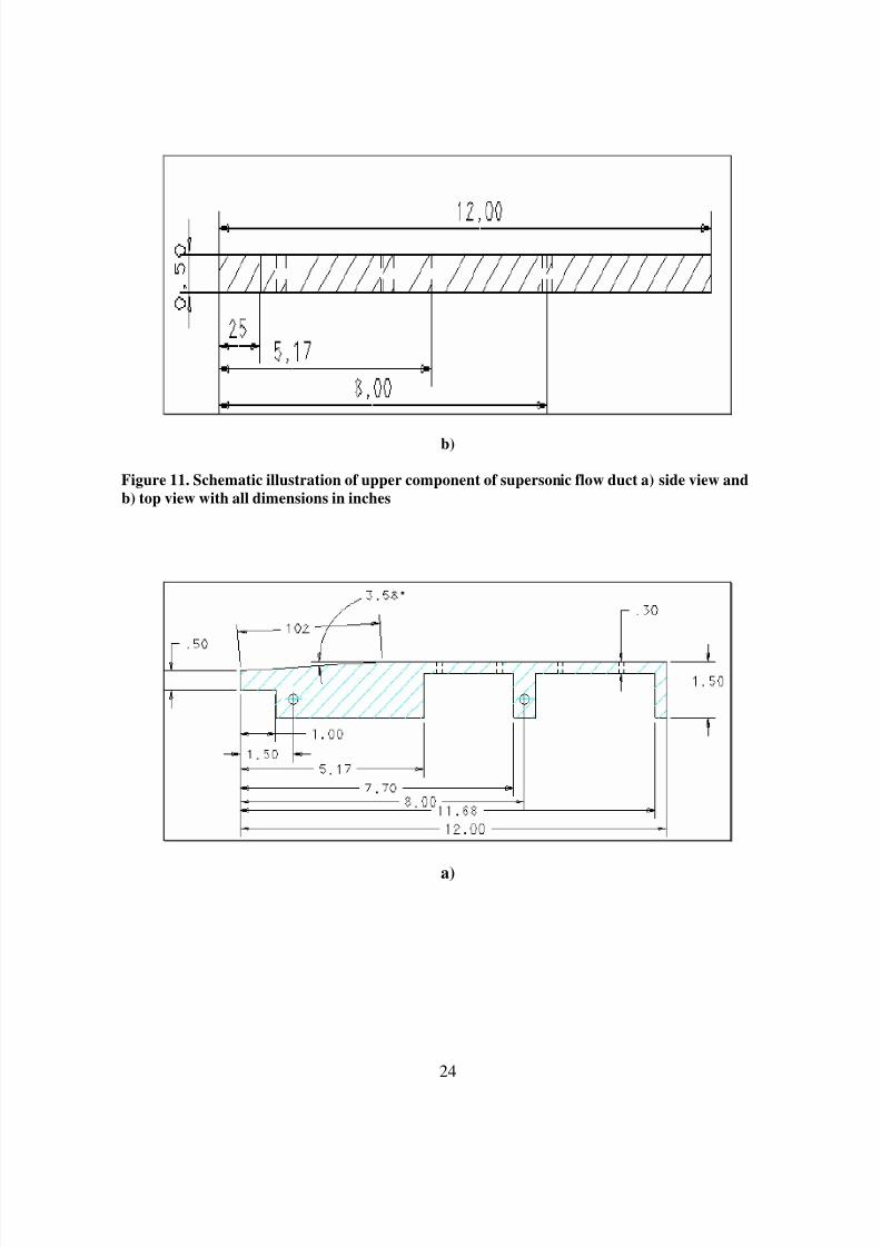
dimensions for the upper and lower components are shown in Figures 11 and 12, respectively. In Figure 11a,
the side view of upper component of the supersonic duct is shown with the very noticeable convergent-
divergent section of the duct.
a)
8/6/2019 umi-umd-3786
http://slidepdf.com/reader/full/umi-umd-3786 40/146
24
b)
Figure 11. Schematic illustration of upper component of supersonic flow duct a) side view and
b) top view with all dimensions in inches
a)

8/6/2019 umi-umd-3786
http://slidepdf.com/reader/full/umi-umd-3786 41/146
25
b)
Figure 12. Schematic illustration of lower component of supersonic flow duct a) side view
and b) top view
The supersonic flow exiting the combustor section is discharged into a 4-in (101.6mm) diameter exhaust pipe
after passing through a series of mounting brackets. This arrangement for supersonic jet exhaust flow resulted
in strong acoustic resonance of the discharged jet under certain conditions, creating high-amplitude screech tone
noise. The mechanism generating screech noise appeared to be related to hole-tone resonance in supersonic
jets. While the study of screech mechanism is not in the scope of current investigation, this phenomenon
allowed us to investigate the transmission and attenuation characteristics of resulting pressure oscillations
through the supersonic duct upstream.
3.2.2. Acoustic Wave Pressure Measurements
Figure 13. Schematic drawing of 2-D view of convergent-divergent supersonic duct depicting
pressure transducer location relative to duct height
Ho
3Ho7Ho
11Ho15Ho
9.4Ho6.7Ho PT1
PT2PT3PT4PT5

8/6/2019 umi-umd-3786
http://slidepdf.com/reader/full/umi-umd-3786 42/146
26
The notation PT1 in Figure 13 denotes the location of the acoustic source designated location point. A typical
schlieren image was imbedded inside the schematic drawing of c-d supersonic duct to illustrate the dynamics of
the flowfield taking place at each pressure transducer. The first 6.7 duct height (6.7Ho) downstream of the
convergent-divergent nozzle corresponds to isolator section, and the remaining 9.4 duct height (9.4Ho) is
analogous to the expanding combustor section. The “combustor” flow then discharges into ambient air and to
the exposed exhaust duct. Again, the test section is equipped with quartz windows where the internal flow can
be visualized using schlieren or shadowgraph flow visualization techniques. As shown in Figure 13, the
transducers were placed at a distance of 3Ho(PT2), 7Ho(PT3), 11Ho(PT4), and 15Ho(PT5), where Ho=0.425in,
away from duct exit. Power and signal conditioning for the pressure transducers were provided by the four
channel Kistler 5134A Power Supply and Signal Conditioner, which essentially serves as an interface between
the piezoelectric pressure transducers and the analyzing instrumentation.
3.3 Flow Visualization Methods
Qualitative investigation of the internal flowfield as well as the acoustic phenomenon at the duct exit was
carried out by using a well known flow visualization technique. Optical techniques are very common
experimental tools for investigating the intricate details of fluid flow. In particular, highly compressible fluid
flows are in a sense ideal for some of these methods due to the fundamental physical principles involve between
the gas flow and the optics. Typically, the three most common methods in flow visualization for compressible
gas flow are the Mach-Zehnder(MZ) interferometer method, the schlieren method, and the shadowgraph.25
In
principle, each one of those methods, afore mentioned, is tied to the physical phenomenon of the speed of light
and its dependency on the index of refraction of the fluid medium as it propagates through. In essence, the
density gradient affects how light bends in the fluid medium because of the index of refraction. The larger the
density gradient of the fluid the larger index of refraction of the medium, hence creating favorable conditions
for flow visualization by optical means. The interferometer method differs from both the shadowgraph and
schlieren techniques with its ability to render reliable quantitative measurements of the density of flowfiled.25

8/6/2019 umi-umd-3786
http://slidepdf.com/reader/full/umi-umd-3786 43/146
27
Other critical difference for the interferometer are its inherent difficulty to operate and being very costly.
The repeating dark and light bands also known as fringes are the distinguishing factors for the interferometer
method in comparison to the shadowgraph and schlieren flow visualization methods. Basically, one is able to
extract the density data based upon these color striations where the darker bands signify higher density and less
density for lighter bands.25
3.3.1. Shadowgraph Method
Of the three flow visualization that focuses on the density change in the flow, the shadowgraph is the simplest
to setup but yields the least amount of concrete information.25
This optical technique focuses on the how light is
refracted as it travels through the compressible flow field. This method is only effective if there is a gradient of
the density gradient in the flow. This can be interpreted as the changes in the brightness pattern on the
photographic surface is direct function of the 2nd
derivative of the density gradient.25
This basically means that
with a constant deflection of light in a constant density gradient flow filed one would observe no change in
brightness of the flowfield. Now, if there exist a gradient of the density gradient inside the flowfield very
distinct flow structures will become apparent on the viewing surface. As a result of this, the shadowgraph has
been a very effective flow visualization technique for observing shock wave patterns in a highly compressible
flowfield.25
It is well know in fluid dynamics that across a shock wave density changes dramatically hence the
change in density will be illuminated instantly with this optical method.24
The general observations are bright
lines that follow dark lines wherever shocks are located, or any rapidly changing region of density gradient.25
In
Figure 14, a typical shadow graph setup is shown where light is projected from a point source then on to a
spherical mirror or through a lens. The light will be collimated, or made parallel, as it passes through the lens or
reflected from the mirror. The collimated rays then travel through the investigation region, where transparent
material such as polished quartz glass serves as boundary surface for the confinement fluid medium and
transmission passage for the collimated light rays on to some type of photographic surface.25

8/6/2019 umi-umd-3786
http://slidepdf.com/reader/full/umi-umd-3786 44/146
28
Figure 14. Schematic drawing of shadowgraph flow visualization method
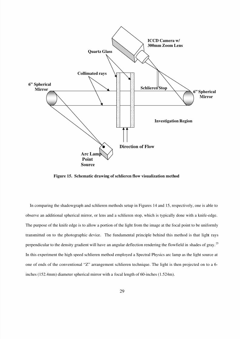
3.3.2. Schlieren Method
For this experiment, the schlieren method was extensively employed to characterize the internal flowfield of the
supersonic duct. In comparison to the MZ-interferometer method, one is able to get, in theory, quantitative
density gradient data but the accuracy is know to be far less reliable than the values obtain using MZ-
interferometer technique.25
The images of the flowfield especially the turbulent structure, vortex structures and
shock waves are more profound using the schlieren method than the MZ-interferometer principle. Unlike the
shadowgraph technique, the shock waves that observed in the schlieren method are not accompanied by dark
and bright lines.25 The basic setup of the shadow graph is very similar to the schlieren setup, but typically two
additional critical components are need for the schlieren setup.
Investigation Region
PhotographicSurface
Glass
Direction of FlowPoint
Source of Light
Spherical
Mirror orLens
Collimated rays
8/6/2019 umi-umd-3786
http://slidepdf.com/reader/full/umi-umd-3786 45/146

8/6/2019 umi-umd-3786
http://slidepdf.com/reader/full/umi-umd-3786 46/146
30
The collimated light rays travel through the test section bounded by two highly polished quartz glass an then on
the second spherical mirror, which has identical physical parameters as the first spherical mirror. From the
second spherical mirror the collimated rays are brought to a focal point where a schlieren stop was intentionally
placed.
A radial schlieren stop was used in order to cut the image at all angles, which rendered a more uniform
distribution of light but at the same time capturing the density gradient in the flow. Two types were used to
capture the images of the flowfield in this experiment. The reason for this arrangement was in part due to the
significant gain in details of the flowfield, which will be evident in the results. The initial camera used was the
Photron Ultima 1024 CMOS camera. This camera operates with an acquisition rate of 60-16000 frames per
seconds (fps) and shutter gate speeds ranging from 0.016 to 7.8x 10⁻⁵ seconds. In this experiment the Photron
camera was operated typically 250 fps and with shutter speeds of 1/32000 seconds. Images rendered by this
camera can be seen in Figures 38 and 39. The second camera that was used during this experiment for schlieren
flow visualization technique was a DiCam Pro camera. The images passing through the radial schlieren stop
was projected on to this intensified charged couple device (ICCD) camera. This specialized CCD camera was
able to significantly capture the flowfield structures in an apparent freeze frame mode due to the high shutter
speed capabilities. Live images of the flowfield were seen on a desktop monitor and then recorded frame-by-
frame using the DiCam software.
3.4 Experimental Methodology
3.4.1. Experimental Approach
Initial characterization of the distinctive acoustic signal emanating from the exit plane of the supersonic duct
was produced using a Tecktronix TDS 3014 digital phosphor oscilloscope. It was conjectured that the
fundamental frequency would be below the 20kHz threshold of the hearing capability of the average person.
With that in mind, it was decided that sampling should be done at a sampling rate that was twice the signal

8/6/2019 umi-umd-3786
http://slidepdf.com/reader/full/umi-umd-3786 47/146
31
frequency in order to not only capture the signal but also reduces the chance of aliasing. Aliasing is well known
as a means of distorting the real signal during the sampling process. Sampling was taken at 250kHz and the
Niquist criterion was effectively executed via the oscilloscope were a complete frequency bandwidth of 125kHz
was captured on the monitor of the oscilloscope. The fluctuation of the signal was averaged using the averaging
mode on the oscilloscope. Essentially this method was designed to reduce the Gaussian noise in the signal such
that the distinct signal of interests can be captured. It is executed in sequential manner where the current signal
is compared to the previous such that abnormalities are discarded as noise and the consistent dominant signal
was rendered.
Once the basic idea of what type of frequency range was expected to be created by the designated test
conditions, a more accurate approach to the data acquisition was carried using Labview. The data acquisition
procedure was carried out with the use of National Instrument (NI) Labview version 6 software. The dynamic
and static pressures were taken simultaneously for 10 consecutive test runs. The flow of data from the Kistler
PiezotronTM
pressure transducers (Model 211B5) inside the duct is illustrated in Figure 15. The pressure
transducers were secured in a flush mounted adapter with a sensor port of approximately 0.1in (2.54mm)
diameter. The pressure transducers are miniature in size, very sensitive, low impedance rating, and high
frequency response. The 211B5 is pressure rated for up to 100psi with frequency range up to 50kHz. The signal
from the pressure transducer is transmitted to the Kistler PiezotronTM
Coupler (Model 5134A). This four
channel input/output piezoelectric sensor power and signal conditioning unit is a robust unit that provides the
necessary excitation and signal processing to each dynamic pressure transducer. The max gain for the
PiezotronTM Coupler is 100 with a bandwidth of 0.036Hz to 10kHz. In this experiment, the gain was set to one
with a higher frequency bandwidth of 30kHz. Cutoff frequency was set to 30kHz for the system imbedded low
pass filter.
For static pressure measurement the raw signal was transmitted from the Setra pressure transducer (Model
206) directly in to the NI-DAQ board. The Setra (Model 206) series pressure transducers are pressure rated up
to 250psig with a response time of 5miliseconds. Pressure values were also displayed on the Datum 2000 TM
dual channel meter. The DAQ board serves as the interface between the Labview software and raw acoustic
signal. Each channel was appropriately scaled for their respective pressure transducers. The sensitivity scaling
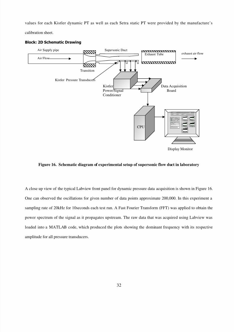
8/6/2019 umi-umd-3786
http://slidepdf.com/reader/full/umi-umd-3786 48/146
32
values for each Kistler dynamic PT as well as each Setra static PT were provided by the manufacture’s
calibration sheet.
Block: 2D Schematic Drawing
Figure 16. Schematic diagram of experimental setup of supersonic flow duct in laboratory
A close up view of the typical Labview front panel for dynamic pressure data acquisition is shown in Figure 16.
One can observed the oscillations for given number of data points approximate 200,000. In this experiment a
sampling rate of 20kHz for 10seconds each test run. A Fast Fourier Transform (FFT) was applied to obtain the
power spectrum of the signal as it propagates upstream. The raw data that was acquired using Labview was
loaded into a MATLAB code, which produced the plots showing the dominant frequency with its respective
amplitude for all pressure transducers.
exhaust air flow
Transition
Air Supply pipe Supersonic Duct
Exhaust Tube
Air Flow
Kistler
Power/Signal
Conditioner
Data Acquisition
Board
CPU
Display Monitor
Kistler Pressure Transducers

8/6/2019 umi-umd-3786
http://slidepdf.com/reader/full/umi-umd-3786 49/146
33
Chapter 4: Results and Discussion
4.1. Internal Flowfield Characterization
4.1.1. Schlieren Images of Prominent Turbulent Flow and Shock Structures
Typical schlieren images of the internal flowfield are shown in Figure 17 for various stagnation pressures
using the DiCAM-ICCD Camera. The region of the supersonic duct depicted in Figure 17 is from the inlet to
the end of the constant area section, or the isolator. It can be seen from Figure 17 that the detailed turbulent and
shock structures of the flowfield become profound as the upstream stagnation pressure increases from 20psig to
110psig. This complicated flowfield can be attributed to the intricate interaction between the boundary layer and
the shock wave taking place along the surface of the duct.25
When the stagnation pressure was relatively low,
the nozzle boundary layer thickness remained small and the oblique shock train was observed inside the isolator
duct. At higher stagnation pressure conditions, the shock train appeared more normal than oblique due to
thicker boundary layer associated with turbulent boundary flow at the nozzle exit. In essence, this is a result of
the development of large adverse pressure gradient due to the normal shock train in the central core of the
stream.25 A backflow in the boundary layer created separation of the stream from the duct walls. These normal
shock trains decelerate the core flow from supersonic to subsonic speeds, while increasing the static pressure
across the shocks. In this experimental setup, the subsonic flow was reaccelerated at the end of the isolator as
the upper wall expanded at a constant angle of 3°.
Normal shock trains, where there are a series of normal shocks in supersonic flow, are typical examples of the
complex flowfield structures that frequently occur in devices such as supersonic wind-tunnels, inlets of
scramjets, as well as supersonic ejectors.35
At high speeds (M>1), these “multiple shock waves” interact with
the turbulent boundary layer (as seen in Figure 17). This interaction, according to Carroll et al.25 has the
potential of producing a non-uniform and unsteady flow conditions downstream of the interaction.
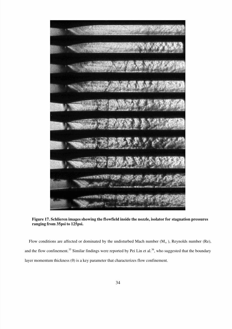
8/6/2019 umi-umd-3786
http://slidepdf.com/reader/full/umi-umd-3786 50/146
34
Figure 17. Schlieren images showing the flowfield inside the nozzle, isolator for stagnation pressuresranging from 35psi to 125psi.
Flow conditions are affected or dominated by the undisturbed Mach number (Mu ), Reynolds number (Re),
and the flow confinement.35 Similar findings were reported by Pei Lin et al.36, who suggested that the boundary
layer momentum thickness () is a key parameter that characterizes flow confinement.
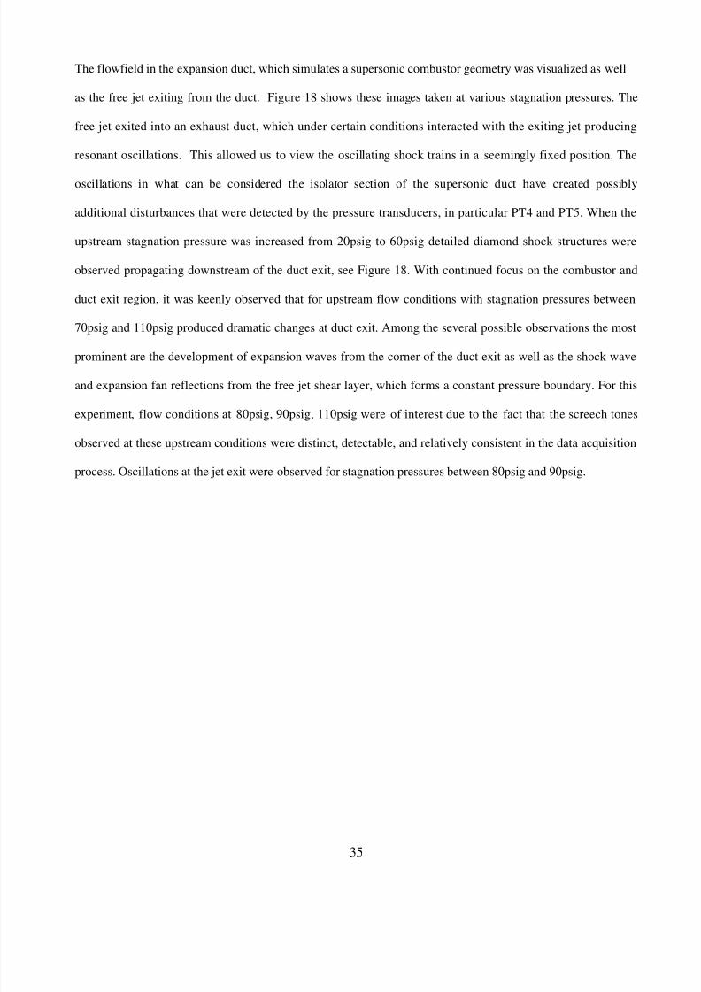
8/6/2019 umi-umd-3786
http://slidepdf.com/reader/full/umi-umd-3786 51/146
35
The flowfield in the expansion duct, which simulates a supersonic combustor geometry was visualized as well
as the free jet exiting from the duct. Figure 18 shows these images taken at various stagnation pressures. The
free jet exited into an exhaust duct, which under certain conditions interacted with the exiting jet producing
resonant oscillations. This allowed us to view the oscillating shock trains in a seemingly fixed position. The
oscillations in what can be considered the isolator section of the supersonic duct have created possibly
additional disturbances that were detected by the pressure transducers, in particular PT4 and PT5. When the
upstream stagnation pressure was increased from 20psig to 60psig detailed diamond shock structures were
observed propagating downstream of the duct exit, see Figure 18. With continued focus on the combustor and
duct exit region, it was keenly observed that for upstream flow conditions with stagnation pressures between
70psig and 110psig produced dramatic changes at duct exit. Among the several possible observations the most
prominent are the development of expansion waves from the corner of the duct exit as well as the shock wave
and expansion fan reflections from the free jet shear layer, which forms a constant pressure boundary. For this
experiment, flow conditions at 80psig, 90psig, 110psig were of interest due to the fact that the screech tones
observed at these upstream conditions were distinct, detectable, and relatively consistent in the data acquisition
process. Oscillations at the jet exit were observed for stagnation pressures between 80psig and 90psig.

8/6/2019 umi-umd-3786
http://slidepdf.com/reader/full/umi-umd-3786 52/146
36
Figure 18. Schlieren images showing the flowfield inside the expansion region of the duct for
stagnation pressures ranging from 35psi to 125psi

8/6/2019 umi-umd-3786
http://slidepdf.com/reader/full/umi-umd-3786 53/146
37
The prominent growth of the shear layers streaming from the duct exit, illustrated Figure 18, for stagnation
pressures between 80psig and 100psig are also of interests. At this pressure range, as previously mentioned, the
occurrences of screech tones were observed. This seems to support Powell’s22
theory of the interaction between
the shear layer and shock cells to create the distinct acoustic phenomena.
4.2. Acoustic Wave Amplitude Characterization
4.2.1 Acoustic Signature Characterization
In Figures 19-22, the acoustic signatures of the supersonic jet stream for four upstream pressure conditions
of interest are illustrated. The distinct acoustic signals were established by the passive acoustic excitation
mechanism at the following pressures: 95psi, 105psi, 115psi, and 125psi. These absolute stagnation values were
chosen because of the simple fact that at these particular stagnation pressure values (+/- 3psi) fundamental
frequencies were captured repeatedly over several characterization experimental test runs. The power spectrum
plots illustrated in Figures 19-22 are typical representations of the numerous spectral analysis results that were
obtained for this investigation, which can be seen in Appendix section. From these figures, one is able to
observe how the acoustic wave pressure amplitude, measured in RMS (root mean square) squared, diminishes
as it travels through the supersonic ducted medium. With increasing upstream stagnation pressure, the
frequency of the dominant acoustic signal decreased from 4.2kHz at 95psi to 2.8kHz at 125psi. It was also
observed that even though there was a significant decrease in frequency going from 95psi to 125psi there was
little or no change in dominant frequency values at 105psi, 115psi, and 125psi. In Figures 19-22, each spectral
analysis plot starts off with power spectrum the first pressure transducer, PT2 (a) that the acoustic waves
encounter in the in duct. With the subsequent plots representing PT3 (b), PT4(c), PT5 (d) as the wave travels
upstream.

8/6/2019 umi-umd-3786
http://slidepdf.com/reader/full/umi-umd-3786 54/146
38
a)
b)
c)
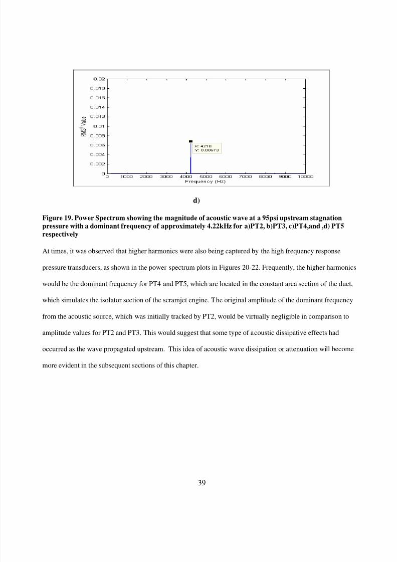
8/6/2019 umi-umd-3786
http://slidepdf.com/reader/full/umi-umd-3786 55/146
39
d)
Figure 19. Power Spectrum showing the magnitude of acoustic wave at a 95psi upstream stagnation
pressure with a dominant frequency of approximately 4.22kHz for a)PT2, b)PT3, c)PT4,and ,d) PT5
respectively
At times, it was observed that higher harmonics were also being captured by the high frequency response
pressure transducers, as shown in the power spectrum plots in Figures 20-22. Frequently, the higher harmonics
would be the dominant frequency for PT4 and PT5, which are located in the constant area section of the duct,
which simulates the isolator section of the scramjet engine. The original amplitude of the dominant frequency
from the acoustic source, which was initially tracked by PT2, would be virtually negligible in comparison to
amplitude values for PT2 and PT3. This would suggest that some type of acoustic dissipative effects had
occurred as the wave propagated upstream. This idea of acoustic wave dissipation or attenuation will become
more evident in the subsequent sections of this chapter.

8/6/2019 umi-umd-3786
http://slidepdf.com/reader/full/umi-umd-3786 56/146
40
a)
b)
c)

8/6/2019 umi-umd-3786
http://slidepdf.com/reader/full/umi-umd-3786 57/146
41
d)
Figure 20. Power Spectrum showing the magnitude of acoustic wave at a 105psi upstream stagnation
pressure with a dominant frequency of approximately 2.79kHz for a)PT2, b)PT3, c)PT4,and ,d) PT5
respectivelyContinuing with the observations of these power spectrum plots, a closer look at the analysis for pressure
transducer locations PT4(c) and PT5(d) for Figures 20-22 would suggest some interestingly acute behavior of
the flowfield’s affect on the acoustic wave or vice versa. One may observe the unique conditions that exist in
the power spectrum plots for both PT4 and PT5 in comparison to the acoustic source, PT2, and PT3 for most of
the upstream pressure conditions under investigation. At these locations, the power spectrum illustrates an
increase in signal intensity, which may be attributed to the oscillations of the normal shock train in the isolator
region. To clarify this point, let’s take a look at Figure 21, as an example. First, one observes the general trend
of decreasing amplitude of the acoustic signal from PT2 (a)-PT5(d). Even though there is an increase in
amplitude for PT5, as opposed to PT4, the relative amplitude in comparison to original encounter at PT2
(0.0017 RMS2) and PT5 (7.487x10⁻⁵ RMS2) has decreased significantly.

8/6/2019 umi-umd-3786
http://slidepdf.com/reader/full/umi-umd-3786 58/146
42
a)
b)
c)

8/6/2019 umi-umd-3786
http://slidepdf.com/reader/full/umi-umd-3786 59/146
43
d)Figure 21. Power Spectrum showing the magnitude of acoustic wave at a 115psi upstream stagnation
pressure with a dominant frequency of approximately 2.78kHz for a)PT2, b)PT3, c)PT4,and ,d) PT5
respectively.
This amount of relative dissipation will be addressed in the next section. Second, both PT4 and PT5 have a
dominant frequency at higher harmonics, approximately 5.6kHz, and what may be described as amplified
erratic signals. With this in mind, one can look back at the corresponding internal flowfield schlieren images in
Figure 17 and see the complex dynamics within this region of inspection. The flowfield becomes extremely
turbulent as the upstream stagnation pressure increases from 35psi to 125psi. For the example above, the
schlieren images at 115psi hints at the complexity of the flowfield, which become numerically evident in the
spectral analysis. Comparing this to a flowfield at 95psi, even though it is relatively turbulent, it is arguably
more turbulent at 115psi..
a)Looking at Figure 19, it can be observed that at PT4 and PT5, the signal intensity is more or less
negligible in comparison to the signals at 115 as well as 125psi in Figures 21 and 22, respectively.

8/6/2019 umi-umd-3786
http://slidepdf.com/reader/full/umi-umd-3786 60/146
44
b)
c)
d)
Figure 22. Power Spectrum showing the magnitude of acoustic wave at a 125psi upstream stagnation
pressure with a dominant frequency of approximately 2.78kHz for a)PT2, b)PT3, c)PT4,and ,d) PT5

8/6/2019 umi-umd-3786
http://slidepdf.com/reader/full/umi-umd-3786 61/146
45
The distinct shock structures coupled with a dominant turbulent flowfield with a mixture of shock/ boundary
layer interactions would be strong evidence for this amplified erratic dynamic pressure signals occurring at PT4
and PT5. What seems to be encouraging is that the acoustic intensity will decrease but over what distance of
which further investigation and analysis will be needed. These power spectrums are clear indicators that the
large amplitude pressure oscillations in combustors of scramjet engines will more than likely propagate through
the subsonic region of the supersonic core flow, namely the boundary layer.
4.2.2. Amplitude Attenuation
The general trend of the dissipation of acoustic intensity as the upstream stagnation pressure increases is
illustrated in Figure 23. In this figure, the analysis of the dynamic pressure signal was carried out for absolute
stagnation pressure values of 95psi, 105psi, 115psi, and 125psi. The data points are based on ten sequential
experimental runs for each upstream stagnation pressure conditions stated above.
a)
Ho
CombustorIsolator PT1
PT2PT3PT4PT5
Air Flow
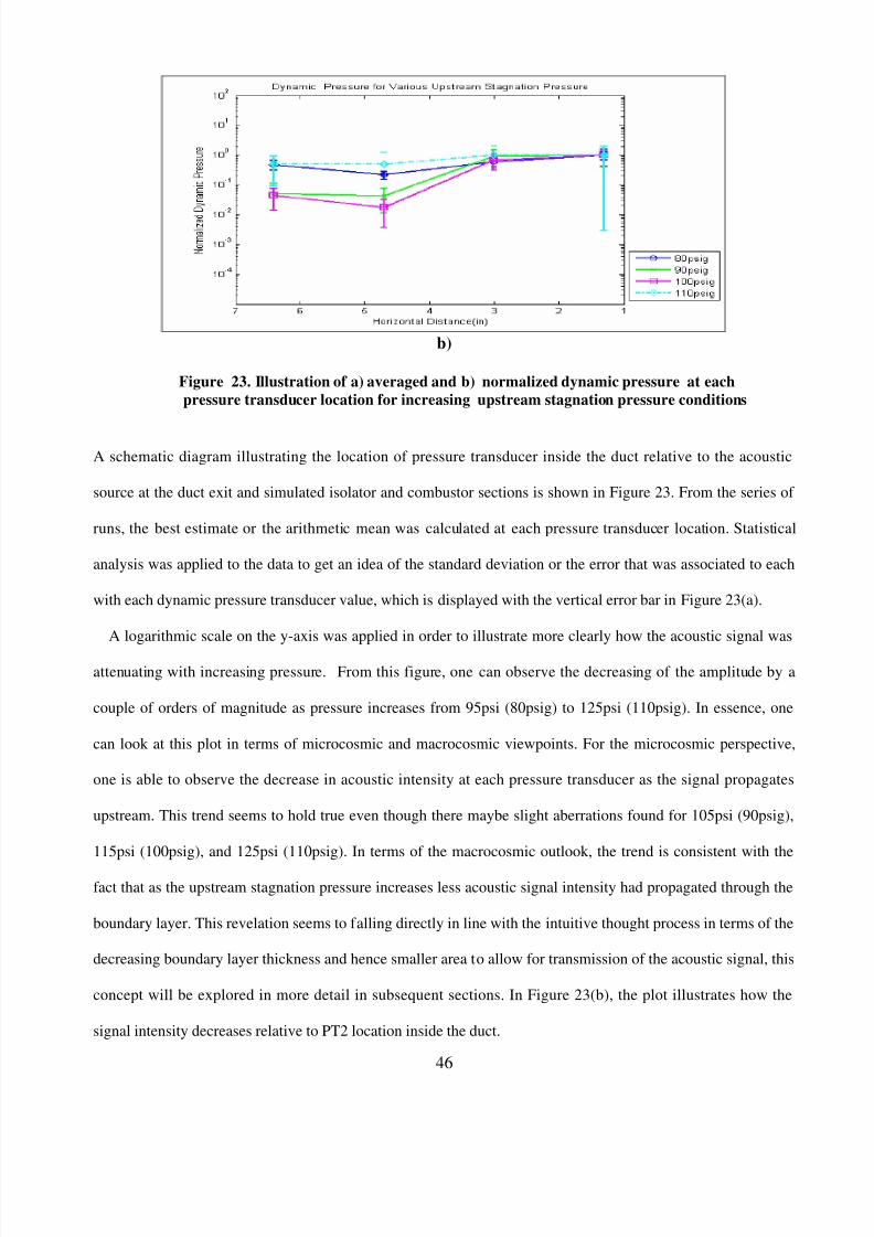
8/6/2019 umi-umd-3786
http://slidepdf.com/reader/full/umi-umd-3786 62/146
46
b)
Figure 23. Illustration of a) averaged and b) normalized dynamic pressure at each
pressure transducer location for increasing upstream stagnation pressure conditions
A schematic diagram illustrating the location of pressure transducer inside the duct relative to the acoustic
source at the duct exit and simulated isolator and combustor sections is shown in Figure 23. From the series of
runs, the best estimate or the arithmetic mean was calculated at each pressure transducer location. Statistical
analysis was applied to the data to get an idea of the standard deviation or the error that was associated to each
with each dynamic pressure transducer value, which is displayed with the vertical error bar in Figure 23(a).
A logarithmic scale on the y-axis was applied in order to illustrate more clearly how the acoustic signal was
attenuating with increasing pressure. From this figure, one can observe the decreasing of the amplitude by a
couple of orders of magnitude as pressure increases from 95psi (80psig) to 125psi (110psig). In essence, one
can look at this plot in terms of microcosmic and macrocosmic viewpoints. For the microcosmic perspective,
one is able to observe the decrease in acoustic intensity at each pressure transducer as the signal propagates
upstream. This trend seems to hold true even though there maybe slight aberrations found for 105psi (90psig),
115psi (100psig), and 125psi (110psig). In terms of the macrocosmic outlook, the trend is consistent with the
fact that as the upstream stagnation pressure increases less acoustic signal intensity had propagated through the
boundary layer. This revelation seems to falling directly in line with the intuitive thought process in terms of the
decreasing boundary layer thickness and hence smaller area to allow for transmission of the acoustic signal, this
concept will be explored in more detail in subsequent sections. In Figure 23(b), the plot illustrates how the
signal intensity decreases relative to PT2 location inside the duct.

8/6/2019 umi-umd-3786
http://slidepdf.com/reader/full/umi-umd-3786 63/146
47
This location was the chosen point of reference, therefore the all values were normalized with respect to
PT2’s measured acoustic pressure. If one follows the lines on the graph going from right to left starting at PT2,
it can be observed that at each subsequent location after PT2 there is an order of magnitude decrease in original
intensity at PT2. The relatively small error gaps at all locations for the respective pressure conditions give a
certain level of confidence in the overall trend of the attenuation effects. In essence, the tracking was done such
that the fundamental frequency of the acoustic signal was detected at each pressure transducer location and the
amplitude of that frequency was observed to be in general smaller than the acoustic signal at PT2. As afore-
mentioned, the general trend is that the signal does dissipate from PT2 to PT5, if we look at the trend from PT4
to PT5 the amplitude generally increases.
A similar graphical layout to Figure 23 is shown in Figure 24 for the static pressure measurements and the ratio
of the dynamic pressure to the static pressure measurements. The arithmetic mean of the static pressure was
analyzed based on approximately 90 static pressure measurements taken simultaneously at each location. The
standard deviations of these values were calculated and plotted with the best estimate for upstream pressure
conditions under consideration, see Figure 24.
a)
Air Flow
Ho
CombustorIsolator PT1
PT2PT3PT4PT5
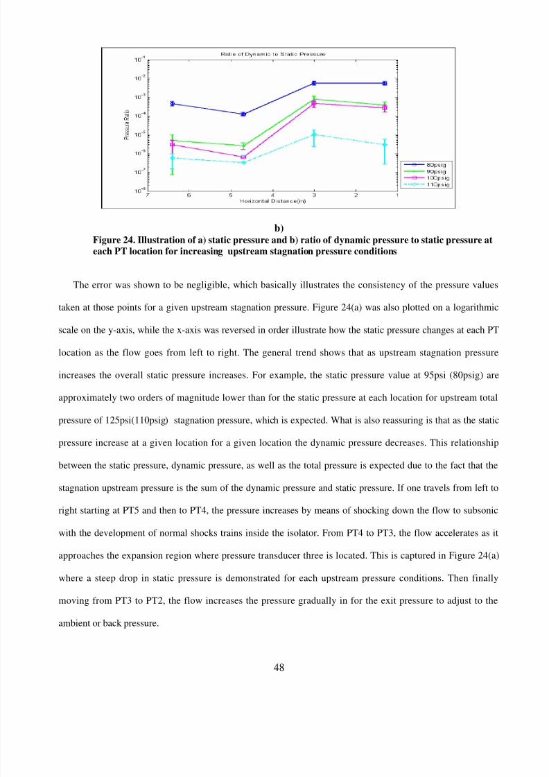
8/6/2019 umi-umd-3786
http://slidepdf.com/reader/full/umi-umd-3786 64/146
48
b)Figure 24. Illustration of a) static pressure and b) ratio of dynamic pressure to static pressure at
each PT location for increasing upstream stagnation pressure conditions
The error was shown to be negligible, which basically illustrates the consistency of the pressure values
taken at those points for a given upstream stagnation pressure. Figure 24(a) was also plotted on a logarithmic
scale on the y-axis, while the x-axis was reversed in order illustrate how the static pressure changes at each PT
location as the flow goes from left to right. The general trend shows that as upstream stagnation pressure
increases the overall static pressure increases. For example, the static pressure value at 95psi (80psig) are
approximately two orders of magnitude lower than for the static pressure at each location for upstream total
pressure of 125psi(110psig) stagnation pressure, which is expected. What is also reassuring is that as the static
pressure increase at a given location for a given location the dynamic pressure decreases. This relationship
between the static pressure, dynamic pressure, as well as the total pressure is expected due to the fact that the
stagnation upstream pressure is the sum of the dynamic pressure and static pressure. If one travels from left to
right starting at PT5 and then to PT4, the pressure increases by means of shocking down the flow to subsonic
with the development of normal shocks trains inside the isolator. From PT4 to PT3, the flow accelerates as it
approaches the expansion region where pressure transducer three is located. This is captured in Figure 24(a)
where a steep drop in static pressure is demonstrated for each upstream pressure conditions. Then finally
moving from PT3 to PT2, the flow increases the pressure gradually in for the exit pressure to adjust to the
ambient or back pressure.
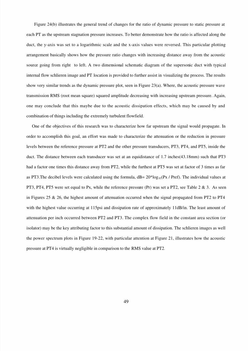
8/6/2019 umi-umd-3786
http://slidepdf.com/reader/full/umi-umd-3786 65/146
49
Figure 24(b) illustrates the general trend of changes for the ratio of dynamic pressure to static pressure at
each PT as the upstream stagnation pressure increases. To better demonstrate how the ratio is affected along the
duct, the y-axis was set to a logarithmic scale and the x-axis values were reversed. This particular plotting
arrangement basically shows how the pressure ratio changes with increasing distance away from the acoustic
source going from right to left. A two dimensional schematic diagram of the supersonic duct with typical
internal flow schlieren image and PT location is provided to further assist in visualizing the process. The results
show very similar trends as the dynamic pressure plot, seen in Figure 23(a). Where, the acoustic pressure wave
transmission RMS (root mean square) squared amplitude decreasing with increasing upstream pressure. Again,
one may conclude that this maybe due to the acoustic dissipation effects, which may be caused by and
combination of things including the extremely turbulent flowfield.
One of the objectives of this research was to characterize how far upstream the signal would propagate. In
order to accomplish this goal, an effort was made to characterize the attenuation or the reduction in pressure
levels between the reference pressure at PT2 and the other pressure transducers, PT3, PT4, and PT5, inside the
duct. The distance between each transducer was set at an equidistance of 1.7 inches(43.18mm) such that PT3
had a factor one times this distance away from PT2, while the furthest at PT5 was set at factor of 3 times as far
as PT3.The decibel levels were calculated using the formula, dB= 20*log10(Px / Pref). The individual values at
PT3, PT4, PT5 were set equal to Px, while the reference pressure (Pr) was set a PT2, see Table 2 & 3. As seen
in Figures 25 & 26, the highest amount of attenuation occurred when the signal propagated from PT2 to PT4
with the highest value occurring at 115psi and dissipation rate of approximately 11dB/in. The least amount of
attenuation per inch occurred between PT2 and PT3. The complex flow field in the constant area section (or
isolator) may be the key attributing factor to this substantial amount of dissipation. The schlieren images as well
the power spectrum plots in Figure 19-22, with particular attention at Figure 21, illustrates how the acoustic
pressure at PT4 is virtually negligible in comparison to the RMS value at PT2.

8/6/2019 umi-umd-3786
http://slidepdf.com/reader/full/umi-umd-3786 66/146
50
a)
b)
c)
Figure 25. Illustration of rate of the amplitude dissipation (decibels per inch) for specific
upstream stagnation pressures between a)PT2-PT3, b)PT2-PT4, and c) PT2-PT5
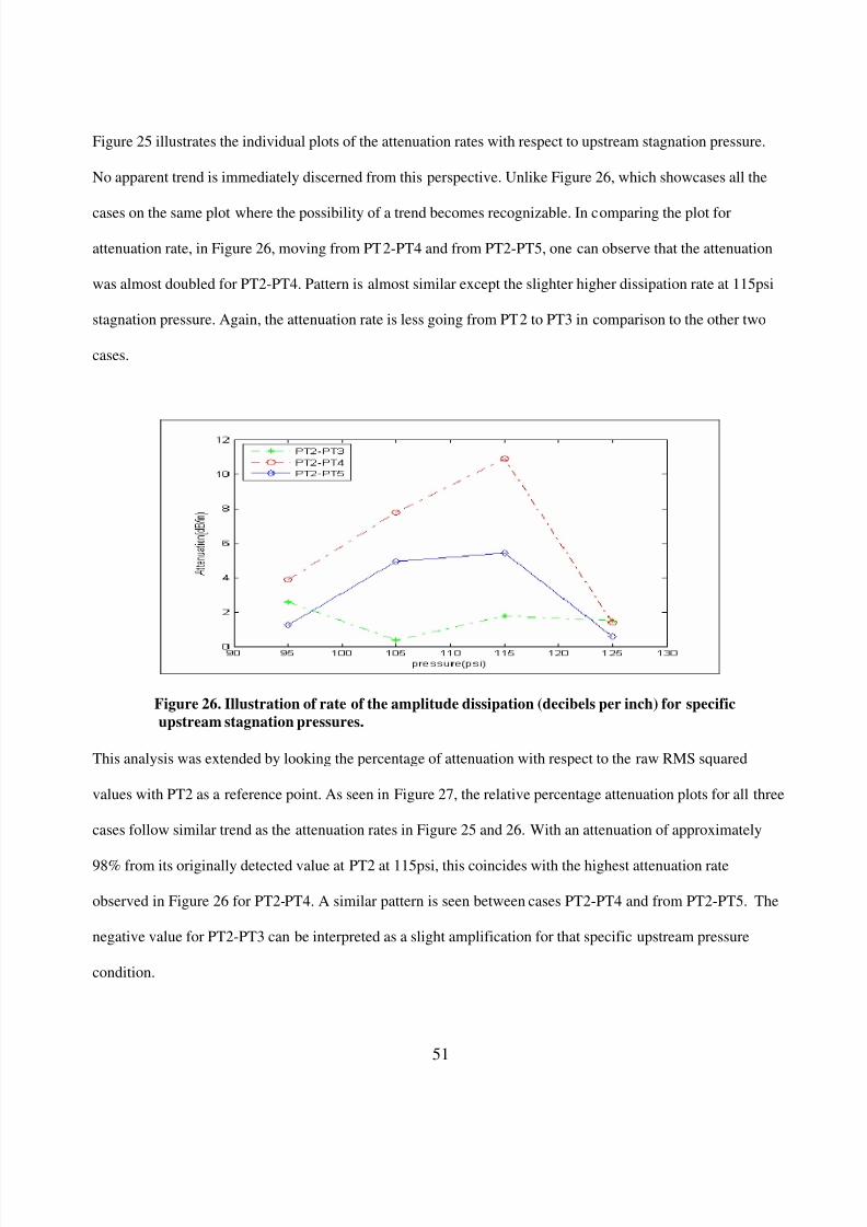
8/6/2019 umi-umd-3786
http://slidepdf.com/reader/full/umi-umd-3786 67/146

8/6/2019 umi-umd-3786
http://slidepdf.com/reader/full/umi-umd-3786 68/146
52
Figure 27. Illustration of relative percentage of the dissipation of acoustic wave amplitude
for various stagnation pressures.
To shed some light on some of the possible reasons for this attenuation effect, the schematic diagram shown in
Figure 28 will be used as an aid.37 According to Hersh et al., Pridmore and Brown [3]37 were pioneers in the late
1950’s for the investigation on how acoustic waves are influenced by shear flow inside a rectangular duct.
Figure 28. Schematic diagram illustrating disturbance propagation in thea) downstream direction and b) upstream direction.
a)
b)
Disturbances
turn towards
wall
Duct Flow
Profile
Disturbancesturn away from
wall
Air Flow
Air Flow
Duct Flow
Profile

8/6/2019 umi-umd-3786
http://slidepdf.com/reader/full/umi-umd-3786 69/146
53
Their focus was mainly on how acoustic attenuation occurs in the downstream direction rather than
upstream propagation. The pivotal findings of their research was that the velocity gradient played a crucial role
in forcing the acoustic waves towards the walls of the duct as seen in Figure 28(a).37
It seems that Hersh and
Catton were the first to seriously tackle the idea of upstream propagation in a rectangular duct with shear flow.
Even though this was not explicitly stated in their writings, it was only implied on the basis of their stated
literature review and motivation for their paper.37
Hersh and Catton numerically confirmed Pridmore and
Brown’s idea of downstream propagation and found that for upstream propagation the acoustic waves were
being directed towards the core flow by the velocity changes were inside the flowfield.37
Whether or not
attenuation was occurring wasn’t explicitly state by the authors,37 which look only at the case for max Mach
number of 0.5. Figure 28 may be just a display of the mechanism of what’s going on inside the duct. According
to Schneider38
who look at the supersonic flow case numerically, the acoustic waves will dampen if viscosity
effects are taken into account. In the case of this experimental research effort where the real flow conditions do
imply that viscosity would play a role, one can see that attenuation effects are occurring based on the above
analysis of the dynamic pressure measurements. These measurements are manifested as power spectrum and
acoustic attenuation plots, which are shown above.
4.3. Effects on the Phase of Acoustic Wave
In Figures 29-31, the variation of the phase differences along the duct with the stagnation pressures 95psi,
105psi, 115psi, and 125psi. The phase calculation was conducted using the FFT analysis of the dynamic
pressure for all 10 sequential runs at each pressure transducer.
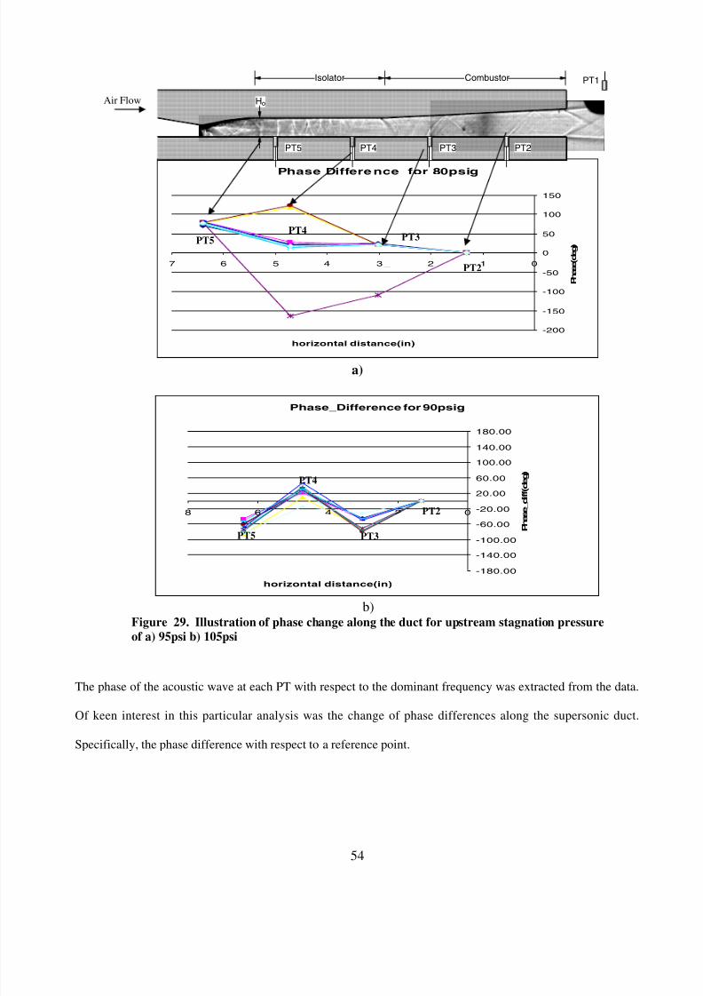
8/6/2019 umi-umd-3786
http://slidepdf.com/reader/full/umi-umd-3786 70/146
54
Phase Differe nce for 80psig
-200
-150
-100
-50
0
50
100
150
01234567
horizontal distance(in)
P h a s e ( d e g )
_
a)
Phase_Difference for 90psig
-180.00
-140.00
-100.00
-60.00
-20.00
20.00
60.00
100.00
140.00
180.00
02468
horizontal distance(in)
P h
a s e_
d i f f ( d e g )
b)Figure 29. Illustration of phase change along the duct for upstream stagnation pressure
of a) 95psi b) 105psi
The phase of the acoustic wave at each PT with respect to the dominant frequency was extracted from the data.
Of keen interest in this particular analysis was the change of phase differences along the supersonic duct.
Specifically, the phase difference with respect to a reference point.
PT2
PT3
PT5
PT2
PT4
PT3
Ho
CombustorIsolator PT1
PT2PT3PT4PT5
PT4
Air Flow
PT5

8/6/2019 umi-umd-3786
http://slidepdf.com/reader/full/umi-umd-3786 71/146
55
Phase_Differe nce for 100psig
-200
-150
-100
-50
0
50
100
150
200
01234567
horizontal distance (in)
P h a s e_
d i f f ( d e g )
a)
Pgase Difference for 110psi
-200
-150
-100
-50
0
50
100
150
200
01234567
horizontal distance(in)
p h a s e d i f f e r e n c e
b)Figure 30. Illustration of phase change along the duct for upstream stagnation pressure
of a)115 psi b) 125psi
The reference point chosen for this analysis was PT2. In order to explore this phase within one cycle, values
were kept within (+/- )180 degree phase. In Figure 29(a), the phase difference at 95psi (80psig) is shown with a
few aberrations from the basic pattern. The relative phase difference going from PT2 to PT3, for all 10
experimental case runs, was on the average 20 degrees with a dominant frequency of approximately 4.8kHz.
PT4
PT5PT2PT3
PT4
PT5PT2PT3
Ho
CombustorIsolator PT1
PT2PT3PT4PT5

8/6/2019 umi-umd-3786
http://slidepdf.com/reader/full/umi-umd-3786 72/146
56
Average Phase Difference
-80.00
-60.00
-40.00
-20.00
0.00
20.00
40.00
60.00
80.00
100.00
01234567
horizontal distance(in)
P h a s e_
d i f f ( d e g )
80psig 90psig 100psig 110psig
Figure 31. Illustration of average phase change along the duct at each pressure transducer
location for increasing upstream stagnation pressure conditions.
Similarly, the phase differences going from PT2 to PT4 were within the range of 14-20 degrees, see Figure
29(a). The phase gap widens by approximately 50 degrees travel from PT2 to PT5. It can be observed that the
trend for almost all the cases were consistent except for a few data points. Now, for the upstream conditions at
105psi (90psig) see Figure 29(b), the negative and positive phase alternation becomes prominent. Also, the
average phase gap between the pressure transducers increased slightly in comparison to those found in Figure
29(a). Even though that may be the case, interestingly enough, it can be observed that all ten experimental case
runs at this pressure condition more or less followed the same phase difference pattern. This could suggest some
type of phase correlation between the points of interest.
In Figure 30, both phase difference trends display what may be construed as some type of oscillation change
around PT4 at 115psi and 125psi. With a dominant frequency of 2.8kHz, the phase difference at 115psi between
PT2 and PT3 is fairly consistent for all case runs with an average phase difference of approximately 37 degrees.
In Figure 30(b) the variation gap widens with an average difference of approximately minus 48 degrees. The
seemingly sporadic behavior is the same for both pressure conditions going from PT2 to PT4 and PT2 to PT5,
with the largest phase difference (73 degrees) occurring at PT2-PT4. To further extending this analysis, the
Ho
CombustorIsolator PT1
PT2PT3PT4PT5
Air Flow

8/6/2019 umi-umd-3786
http://slidepdf.com/reader/full/umi-umd-3786 73/146
57
average of all experimental runs were calculated and plotted, see Figure 31. The general pattern alternated
between approximately 80 degrees occurring at PT4 and minus 70 degrees, which occurred at PT5.
4.4. Boundary Layer Thickness Characterization
4.4.1. Upstream Flow conditions
In theory, it is possible to have acoustic waves propagate upstream via boundary layer because a part of the
boundary layer will always remain subsonic no matter how high the value of the core Mach number. However,
it is also expected that, even if the acoustic waves can propagate upstream, there will be substantial attenuation
in the amplitude because the subsonic region is relatively thin and the nature of turbulent boundary layer flow is
very unsteady.
Figure 32. Illustration of boundary layer thickness growth along a flat plate
The turbulent boundary analysis was done on the basis of a first cut approximation modeled with flow over a
flat plate. In Figure 32, a schematic drawing shows the development of the boundary layer as a function of the
horizontal distance x. Given some freestream velocity, a velocity profile is created were the velocity gradient is
prominent inside the boundary layer.
(x)
U
x
U
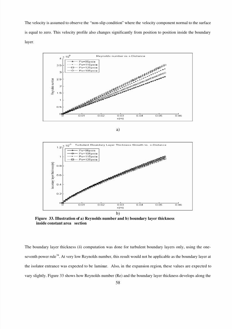
8/6/2019 umi-umd-3786
http://slidepdf.com/reader/full/umi-umd-3786 74/146
58
The velocity is assumed to observe the “non-slip condition” where the velocity component normal to the surface
is equal to zero. This velocity profile also changes significantly from position to position inside the boundary
layer.
a)
b)Figure 33. Illustration of a) Reynolds number and b) boundary layer thicknessinside constant area section
The boundary layer thickness () computation was done for turbulent boundary layers only, using the one-
seventh power rule34
. At very low Reynolds number, this result would not be applicable as the boundary layer at
the isolator entrance was expected to be laminar. Also, in the expansion region, these values are expected to
vary slightly. Figure 33 shows how Reynolds number (Re) and the boundary layer thickness develops along the

8/6/2019 umi-umd-3786
http://slidepdf.com/reader/full/umi-umd-3786 75/146
59
horizontal axis in the constant area section of the duct where pressure transducers 4 and 5 are located. Figure
33(a) shows how Reynolds number increases with the increase in upstream stagnation pressure with values as
high as approximately 3.6 x 10⁶
for 125psi, while the expected turbulent boundary layer thickness decreases in
the constant area section as pressure increases. Also the displacement thickness also shows the similar trend as
the boundary layer thickness, where there is generally a decrease in the displacement thickness (*
disp) as
pressure increase, see Figure 34.
Figure 34. Illustration of turbulent displacement thickness growth inside constant area
section (isolator region)
4.4.2. Boundary Layer and Displacement Growth at Pressure Transducer Location
From the investigation on how the boundary layer thickness and displacement thickness changes continuously
along the horizontal axis inside the constant area, the analysis was than focused more at the what were changes
in boundary layer and displacement thicknesses at the individual pressure transducer locations, in particular at
the specific transducer location. In order to get an idea were the flow transition from laminar became turbulent
as the upstream pressure increased, the critical length was determined, see Figure 35. Typically, the transition to
turbulent can be considered to have occurred when the Reynolds number34
is greater than 500, 000. It was
observed that the transition point from laminar to turbulent occurred less than 0.4 inches(8mm) from the c-d
nozzle exit at max pressure(125psi). As shown in Figure 36, the thickness growth at PT5 with respect to all
pressure conditions showed minute changes. The boundary layer thickness () as well as the displacement

8/6/2019 umi-umd-3786
http://slidepdf.com/reader/full/umi-umd-3786 76/146
60
thickness (*disp) is relatively significant at PT4. Similar observations were made for the displacement thickness
shown in Figure 37.
Figure 35. Illustration of critical length as function of Reynolds number inside constant area
section (isolator region)
Figure 36. Calculated boundary layer thickness growth at pressure transducer locations
PT4 and PT5
Where the ranges from approximately (1.0 x 10⁻³ to 0.971 x 10⁻³ ) meters, see Fig. 36, for upstream pressure
95 to 25psi, respectively. Similarly in Fig. 37, the (*disp) ranges from approximately (1.28 x 10
-4to 1.21 x 10
-4)
meters with 95 to 125psi, respectively.
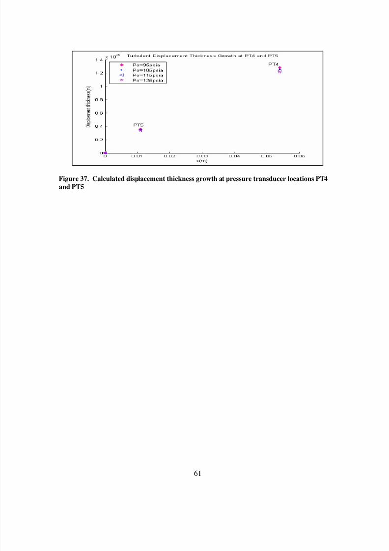
8/6/2019 umi-umd-3786
http://slidepdf.com/reader/full/umi-umd-3786 77/146
61
Figure 37. Calculated displacement thickness growth at pressure transducer locations PT4
and PT5

8/6/2019 umi-umd-3786
http://slidepdf.com/reader/full/umi-umd-3786 78/146
62
Chapter 5: Summary and Conclusion
This research effort was carried out to fully examine whether or not acoustic waves could propagate upstream
through a scramjet internal flowpath. Several non-reacting and passively-controlled experiments were
conducted in a combined supersonic duct-resonant supersonic jet configuration, which simulated the
instabilities in scramjet combustor. Coherent pressure oscillations at several distinct frequencies, which were
generated from supersonic jet screech phenomena at the duct exit, were systematically observed propagating
upstream using wall-mounted pressure transducers. Boundary layer analysis was based on the model of flow
over a flat plate. The natural frequency of the supersonic duct was determined not to be equivalent to the
resonance frequency of the passive acoustic mechanism. Hence, reducing the possible influence on the upstream
propagating wave. To summarize the results of this experiment, the focus was on the following topics:
• Internal Flowfield Characterization
Characterization of the flowfield inside the supersonic duct was carried out using the schlieren method
It can be seen from Figure 17 that the turbulent flow and shock structures of the flowfield inside the constant
area section became more profound as the upstream stagnation pressure increases from 20psig to 110psig. This
complicated flowfield can be attributed to the intricate interaction between the boundary layer and the shock
wave taking place along the surface of the duct.25 When the stagnation pressure was relatively low, the nozzle
boundary layer thickness remained small and the oblique shock train was observed inside the isolator duct. At
higher stagnation pressure conditions, the shock train transitioned to normal shocks due to thicker boundary
layer associated with turbulent boundary flow at the nozzle exit
The flowfield in the expansion duct and the free jet at the duct exit was visualized. Figure 18 shows these
images taken at various stagnation pressures. When the upstream stagnation pressure was increased from 20psig
to 60psig detailed diamond shock structures were observed propagating downstream of the duct exit, see Figure
18. Among the several possible observations the most prominent are the development of expansion waves from
the corner of the duct exit as well as the shock wave and expansion fan reflections from the free jet shear layer,
which forms a constant pressure boundary.

8/6/2019 umi-umd-3786
http://slidepdf.com/reader/full/umi-umd-3786 79/146
63
• Acoustic Wave Amplitude Characterization
An acoustic signature characterization was carried out by performing a spectral analysis of the acoustic
signal. Results from the spectral analysis show the amount of amplitude dissipation as the acoustic wave
traveled upstream. In addition, higher harmonics at time became the dominant frequency various stagnation
pressures. Acute behavior in the flowfield was detected in the constant area section which could be attributable
to the significant reduction in RMS2
value, which was observed at the two extreme upstream pressure
transducer locations. Dynamic pressure measurements show that there is a definite general trend of acoustic
attenuation that is occurring as the signal propagates upstream through the subsonic boundary layer. Normalized
dynamic pressure calculations showcase this attenuation more clearly with reference point taken at PT2. High
attenuation rate up to 11dB/in were observed between the extreme ends of the interrogation region. Again, the
flowfield conditions inside isolator could have a significant role on these attenuation effects. On the basis of
percent attenuation, high percentage (up to 98%) of signal reduction was obtained for pressures such as 105psi
and 115psi.
• Effects of Acoustic Wave Amplitude and Phase
Phase analysis showed that there is a strong correlation between the pressure transducer locations as the signal
propagates upstream. The phase calculations at stagnation pressures 95psi, 105psi, 115psi, and 125psi. were
conducted using the FFT analysis of the dynamic pressure . The analysis focused on the phase difference with
respect to a reference point. The reference point chosen for this analysis was at pressure transducer two (PT2).
The relative phase difference going from PT2 to PT3, for all 10 experimental case runs, was on the average 20
degrees with a dominant frequency of approximately 4.8kHz. The phase gap widens by approximately 50
degrees travel from PT2 to PT5. It can be observed that the trend for almost all the cases were consistent except
for a few data points. The upstream conditions at 105psi (90psig) had an increase in the average phase gap
between the pressure transducers. All sequential runs followed the same general phase difference pattern. This
could suggest some type of phase correlation between the points of interest. With a dominant frequency of
2.8kHz, the phase difference at 115psi between PT2 and PT3 is fairly consistent for all case runs with an
average phase difference of approximately 37 degrees. In Figure 30(b) the variation gap widens with an average
difference of approximately minus 48 degrees.

8/6/2019 umi-umd-3786
http://slidepdf.com/reader/full/umi-umd-3786 80/146
64
• Boundary Layer Thickness Characterization
A first cut turbulent boundary layer analysis of the constant area section shows that Reynolds number increasing
with increase upstream stagnation pressure. Simultaneously, it was observed that the boundary layer thickness
() and displacement thickness (*disp) were decreasing. This could shed some light on why the dynamic
pressure values were decreased overall as the pressure increased due to the reduction of the subsonic boundary
layer channel area.
In theory, it is possible to have acoustic waves propagate upstream via boundary layer because a part of the
boundary layer will always remain subsonic no matter how high the value of the core Mach number. However,
it is also expected that, even if the acoustic waves can propagate upstream, there will be substantial attenuation
in the amplitude because the subsonic region is relatively thin and the nature of turbulent boundary layer flow is
very unsteady. The boundary layer thickness () computation was done for turbulent boundary layers only,
using the one-seventh power rule34. The Reynolds number increases with the increase in upstream stagnation
pressure with values as high as approximately 3.6 x 10⁶
for 125psi, while the expected turbulent boundary layer
thickness decreases in the constant area section as pressure increases. Also the displacement thickness also
shows the similar trend as the boundary layer thickness, where there is generally a decrease in the displacement
thickness (*disp) as pressure increase. It was observed that the transition point from laminar to turbulent
occurred less than 0.4 inches(8mm) from the c-d nozzle exit at max pressure (125psi). The boundary layer
thickness () as well as the displacement thickness (*disp) is relatively significant at PT4.
• Key Findings:
It was found that even though the core flow of the simulated scramjet remained supersonic, pressure
oscillations could still propagate upstream through the boundary layer, part of which would remain
subsonic. This result suggests that a scramjet combustor may be susceptible to acoustic-feedback type self-
sustained combustion instabilities.

8/6/2019 umi-umd-3786
http://slidepdf.com/reader/full/umi-umd-3786 81/146
65
Chapter 6: Future Work
This experimental work, as far as I know, has never been explored before experimentally. A few
drawbacks existed in this preliminary effort to extract the proper physical understand of how the
acoustic signal propagates through the boundary layer in a supersonic flowfield. Therefore continuous
effort is needed to expand this research for more accurate description as well as prediction of
propagation mechanism will be desperately needed. For example, the current experimental setup and
limited scope of the experimental equipment to quantify the boundary layer thickness growth with
respect to the acoustic attenuation such that an applicable relationship can be obtained. In addition, due
to the dimensions of the duct, it was more or less plagued with 3-D effects, which were not accounted
for in this experiment. Therefore, it was difficult to obtain a proper theoretical prediction of the neither
the boundary layer growth nor displacement thickness. The ability to accurately obtain the amplitude
of the acoustic source can further improve this experiment. A collaborative effort with computational
analysis could produce a prediction model. In essence, this research effort has provided more of a
general trend of what one could expect from similar situations.

8/6/2019 umi-umd-3786
http://slidepdf.com/reader/full/umi-umd-3786 82/146
66
Appendices
Figure 38. A Photron Fastcam depicts schlieren images of the flowfield inside the nozzle, isolator, and
expansion zone at stagnation pressure of (a) 35psi, (b) 45psi, (c) 55psi, (d) 75psi, (e) 95psi, (f) 105psi, and
(g) 115psi

8/6/2019 umi-umd-3786
http://slidepdf.com/reader/full/umi-umd-3786 83/146
67
Figure 39. A Photron Fastcam depicts schlieren images of the flowfield inside expansion zone and duct
exit for stagnation pressure of (a) 75psi, (b) 85psi, (c) 95psi, (d) 105psi, (e) 115psi

8/6/2019 umi-umd-3786
http://slidepdf.com/reader/full/umi-umd-3786 84/146
68
Qualitative view of BL growth
Throat to Isolator Region:
• Schlieren Images with knife edge stop(approaching from the bottom)
Figure 40. Qualitative illustration of boundary layer growth inside the constant area section
with upstream pressures from top to bottom: a) 35, b) 45, c)55, d) 65, e)75, f)85, g)95, h)105, i)115, j)125

8/6/2019 umi-umd-3786
http://slidepdf.com/reader/full/umi-umd-3786 85/146
69
From Isolator Exit to Combustor and Nozzle Region:
• Schlieren Images with knife edge stop(approaching from the bottom)
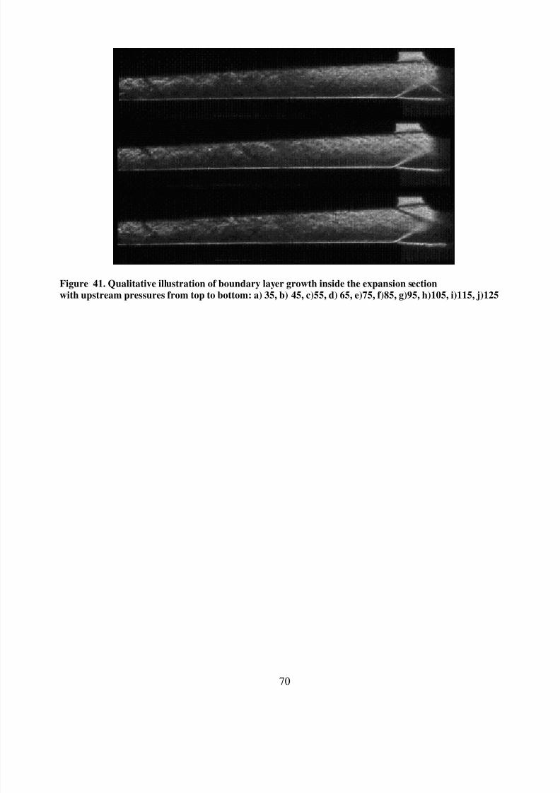
8/6/2019 umi-umd-3786
http://slidepdf.com/reader/full/umi-umd-3786 86/146
70
Figure 41. Qualitative illustration of boundary layer growth inside the expansion section
with upstream pressures from top to bottom: a) 35, b) 45, c)55, d) 65, e)75, f)85, g)95, h)105, i)115, j)125

8/6/2019 umi-umd-3786
http://slidepdf.com/reader/full/umi-umd-3786 87/146
71
Nozzle Exit Region:
• Schlieren Images with apperature
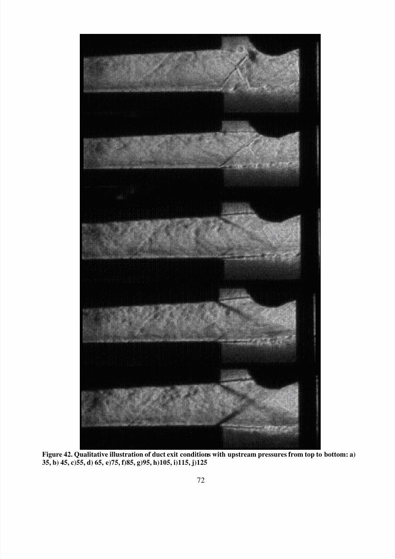
8/6/2019 umi-umd-3786
http://slidepdf.com/reader/full/umi-umd-3786 88/146
72
Figure 42. Qualitative illustration of duct exit conditions with upstream pressures from top to bottom: a)
35, b) 45, c)55, d) 65, e)75, f)85, g)95, h)105, i)115, j)125

8/6/2019 umi-umd-3786
http://slidepdf.com/reader/full/umi-umd-3786 89/146
73
Case Run1
a)
b)
c)
d)Figure 43. Power spectrum of dynamic acoustic signal at 95psi for a)PT2, b)PT3,
c)PT4, and d) PT5 for case run No. 1
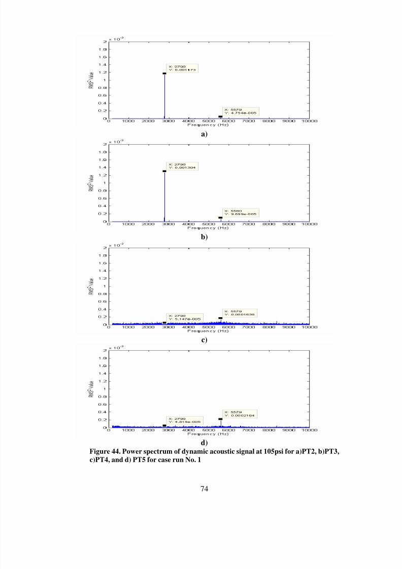
8/6/2019 umi-umd-3786
http://slidepdf.com/reader/full/umi-umd-3786 90/146
74
a)
b)
c)
d)Figure 44. Power spectrum of dynamic acoustic signal at 105psi for a)PT2, b)PT3,
c)PT4, and d) PT5 for case run No. 1

8/6/2019 umi-umd-3786
http://slidepdf.com/reader/full/umi-umd-3786 91/146
75
a)
b)
c)
d)Figure 45. Power spectrum of dynamic acoustic signal at 115psi for a)PT2, b)PT3,
c)PT4, and d) PT5 for case run No. 1
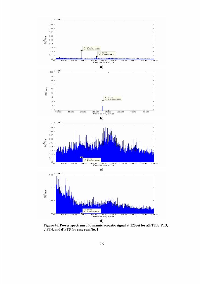
8/6/2019 umi-umd-3786
http://slidepdf.com/reader/full/umi-umd-3786 92/146
76
a)
b)
c)
d)Figure 46. Power spectrum of dynamic acoustic signal at 125psi for a)PT2, b)PT3,
c)PT4, and d)PT5 for case run No. 1

8/6/2019 umi-umd-3786
http://slidepdf.com/reader/full/umi-umd-3786 93/146
77
Case Run2
a)
b)
c)
d)Figure 47. Power spectrum of dynamic acoustic signal at 95psi for a)PT2, b)PT3,
c)PT4, and d) PT5 for case run No. 2

8/6/2019 umi-umd-3786
http://slidepdf.com/reader/full/umi-umd-3786 94/146
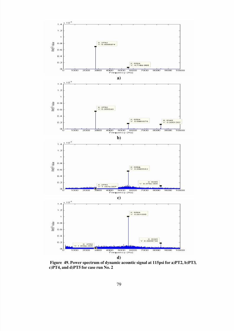
8/6/2019 umi-umd-3786
http://slidepdf.com/reader/full/umi-umd-3786 95/146
79
a)
b)
c)
d)Figure 49. Power spectrum of dynamic acoustic signal at 115psi for a)PT2, b)PT3,
c)PT4, and d)PT5 for case run No. 2
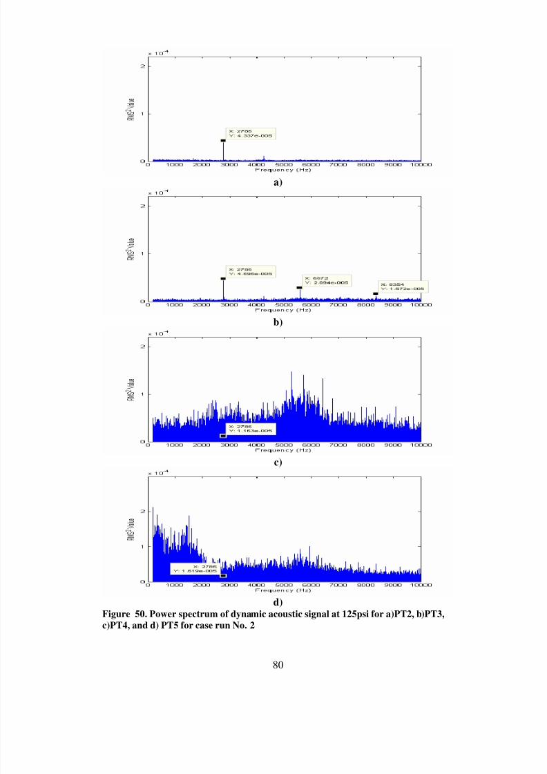
8/6/2019 umi-umd-3786
http://slidepdf.com/reader/full/umi-umd-3786 96/146
80
a)
b)
c)
d)Figure 50. Power spectrum of dynamic acoustic signal at 125psi for a)PT2, b)PT3,
c)PT4, and d) PT5 for case run No. 2
8/6/2019 umi-umd-3786
http://slidepdf.com/reader/full/umi-umd-3786 97/146
81
Case Run3
a)
b)
c)
d)Figure 51. Power spectrum of dynamic acoustic signal at 95psi for a)PT2, b)PT3,
c)PT4, and d) PT5 for case run No. 3

8/6/2019 umi-umd-3786
http://slidepdf.com/reader/full/umi-umd-3786 98/146
82
a)
b)
c)
d)Figure 52. Power spectrum of dynamic acoustic signal at 105psi for a)PT2, b)PT3,
c)PT4, and d) PT5 for case run No. 3

8/6/2019 umi-umd-3786
http://slidepdf.com/reader/full/umi-umd-3786 99/146
83
a)
b)
c)
d)Figure 53. Power spectrum of dynamic acoustic signal at 115psi for a)PT2, b)PT3,
c)PT4, and d) PT5 for case run No. 3
8/6/2019 umi-umd-3786
http://slidepdf.com/reader/full/umi-umd-3786 100/146
84
a)
b)
c)
d)Figure 54. Power spectrum of dynamic acoustic signal at 125psi for a)PT2, b)PT3,
c)PT4, and d) PT5 for case run No. 3
8/6/2019 umi-umd-3786
http://slidepdf.com/reader/full/umi-umd-3786 101/146
85
Case Run4
a)
b)
c)
d)Figure 55. Power spectrum of dynamic acoustic signal at 95psi for a)PT2, b)PT3,
c)PT4, and d) PT5 for case run No. 4

8/6/2019 umi-umd-3786
http://slidepdf.com/reader/full/umi-umd-3786 102/146
86
a)
b)
c)
d)Figure 56. Power spectrum of dynamic acoustic signal at 105psi for a)PT2, b)PT3,
c)PT4, and PT5 for case run No. 4
8/6/2019 umi-umd-3786
http://slidepdf.com/reader/full/umi-umd-3786 103/146
87
a)
b)
c)
d)Figure 57. Power spectrum of dynamic acoustic signal at 115psi for a)PT2, b)PT3,
c)PT4, and d) PT5 for case run No. 4

8/6/2019 umi-umd-3786
http://slidepdf.com/reader/full/umi-umd-3786 104/146

8/6/2019 umi-umd-3786
http://slidepdf.com/reader/full/umi-umd-3786 105/146
89
Case Run5
a)
b)
c)
d)Figure 59. Power spectrum of dynamic acoustic signal at 95psi for a)PT2, b)PT3,
c)PT4, and d) PT5 for case run No. 5

8/6/2019 umi-umd-3786
http://slidepdf.com/reader/full/umi-umd-3786 106/146
90
a)
b)
c)
d)Figure 60. Power spectrum of dynamic acoustic signal at 105psi for a)PT2, b)PT3,
c)PT4, and d) PT5 for case run No. 5

8/6/2019 umi-umd-3786
http://slidepdf.com/reader/full/umi-umd-3786 107/146
91
a)
b)
c)
d)Figure 61. Power spectrum of dynamic acoustic signal at 115psi for a)PT2, b)PT3,
c)PT4, and d) PT5 for case run No. 5

8/6/2019 umi-umd-3786
http://slidepdf.com/reader/full/umi-umd-3786 108/146
92
a)
b)
c)
d)Figure 62. Power spectrum of dynamic acoustic signal at 125psi for a)PT2, b)PT3,
c)PT4, and d) PT5 for case run No. 5
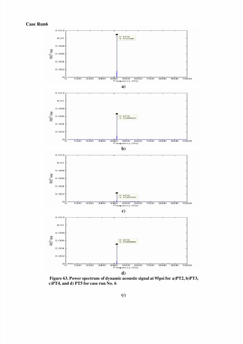
8/6/2019 umi-umd-3786
http://slidepdf.com/reader/full/umi-umd-3786 109/146
93
Case Run6
a)
b)
c)
d)Figure 63. Power spectrum of dynamic acoustic signal at 95psi for a)PT2, b)PT3,
c)PT4, and d) PT5 for case run No. 6

8/6/2019 umi-umd-3786
http://slidepdf.com/reader/full/umi-umd-3786 110/146
94
a)
b)
c)
d)Figure 64. Power spectrum of dynamic acoustic signal at 105psi for a)PT2, b)PT3,
c)PT4, and d) PT5 for case run No. 6

8/6/2019 umi-umd-3786
http://slidepdf.com/reader/full/umi-umd-3786 111/146
95
a)
b)
c)
d)Figure 65. Power spectrum of dynamic acoustic signal at 115psi for a)PT2, b)PT3,
c)PT4, and d) PT5 for case run No. 6

8/6/2019 umi-umd-3786
http://slidepdf.com/reader/full/umi-umd-3786 112/146
96
a)
b)
c)
d)Figure 66. Power spectrum of dynamic acoustic signal at 125psi for a)PT2, b)PT3,
c)PT4, and d) PT5 for case run No. 6

8/6/2019 umi-umd-3786
http://slidepdf.com/reader/full/umi-umd-3786 113/146
97
Case Run7
a)
b)
c)
d)Figure 67. Power spectrum of dynamic acoustic signal at 95psi for a)PT2, b)PT3,
c)PT4, and d) PT5 for case run No. 7

8/6/2019 umi-umd-3786
http://slidepdf.com/reader/full/umi-umd-3786 114/146
98
a)
b)
c)
d)
Figure 68. Power spectrum of dynamic acoustic signal at 105psi for a)PT2, b)PT3,
c)PT4, and d) PT5 for case run No. 7

8/6/2019 umi-umd-3786
http://slidepdf.com/reader/full/umi-umd-3786 115/146
99
a)
b)
c)
d)Figure 69. Power spectrum of dynamic acoustic signal at 115psi for a)PT2, b)PT3,c)PT4, and d) PT5 for case run No. 7

8/6/2019 umi-umd-3786
http://slidepdf.com/reader/full/umi-umd-3786 116/146
100
a)
b)
c)
d)Figure 70. Power spectrum of dynamic acoustic signal at 125psi for a)PT2, b)PT3,
c)PT4, and d) PT5 for case run No. 7

8/6/2019 umi-umd-3786
http://slidepdf.com/reader/full/umi-umd-3786 117/146
101
Case Run8
a)
b)
c)
d)Figure 71. Power spectrum of dynamic acoustic signal at 95psi for a)PT2, b)PT3,
c)PT4, and d) PT5 for case run No. 8

8/6/2019 umi-umd-3786
http://slidepdf.com/reader/full/umi-umd-3786 118/146
102
a)
b)
c)
d)Figure 72. Power spectrum of dynamic acoustic signal at 105psi for a)PT2, b)PT3,
c)PT4, and d) PT5 for case run No. 8
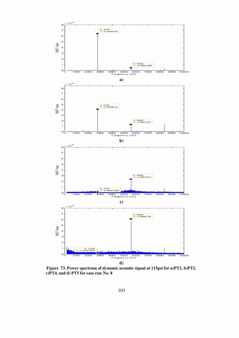
8/6/2019 umi-umd-3786
http://slidepdf.com/reader/full/umi-umd-3786 119/146
103
a)
b)
c)
d)Figure 73. Power spectrum of dynamic acoustic signal at 115psi for a)PT2, b)PT3,
c)PT4, and d) PT5 for case run No. 8

8/6/2019 umi-umd-3786
http://slidepdf.com/reader/full/umi-umd-3786 120/146
104
a)
b)
c)
d)Figure 74. Power spectrum of dynamic acoustic signal at 125psi for a)PT2, b)PT3,
c)PT4, and d) PT5 for case run No. 8

8/6/2019 umi-umd-3786
http://slidepdf.com/reader/full/umi-umd-3786 121/146
105
Case Run9
a)
b)
c)
d)Figure 75. Power spectrum of dynamic acoustic signal at 95psi for a)PT2, b)PT3,
c)PT4, and d) PT5 for case run No. 9

8/6/2019 umi-umd-3786
http://slidepdf.com/reader/full/umi-umd-3786 122/146
106
a)
b)
c)
d)Figure 76. Power spectrum of dynamic acoustic signal at 105psi for a)PT2, b)PT3,
c)PT4, and d) PT5 for case run No. 9

8/6/2019 umi-umd-3786
http://slidepdf.com/reader/full/umi-umd-3786 123/146
107
a)
b)
c)
d)Figure 77. Power spectrum of dynamic acoustic signal at 115psi for a)PT2, b)PT3,
c)PT4, and d) PT5 for case run No. 9

8/6/2019 umi-umd-3786
http://slidepdf.com/reader/full/umi-umd-3786 124/146
108
a)
b)
c)
d)Figure 78. Power spectrum of dynamic acoustic signal at 125psi for a)PT2, b)PT3,
c)PT4, and d) PT5 for case run No. 9

8/6/2019 umi-umd-3786
http://slidepdf.com/reader/full/umi-umd-3786 125/146
109
Case Run10
a)
b)
c)
d)Figure 79. Power spectrum of dynamic acoustic signal at 95psi for a)PT2, b)PT3,
c)PT4, and d) PT5 for case run No. 10

8/6/2019 umi-umd-3786
http://slidepdf.com/reader/full/umi-umd-3786 126/146
110
a)
b)
c)
d)Figure 80. Power spectrum of dynamic acoustic signal at 105psi for a)PT2, b)PT3,
c)PT4, and d) PT5 for case run No. 10

8/6/2019 umi-umd-3786
http://slidepdf.com/reader/full/umi-umd-3786 127/146
111
a)
b)
c)
d)Figure 81. Power spectrum of dynamic acoustic signal at 115psi for a)PT2, b)PT3,
c)PT4, and d) PT5 for case run No. 10
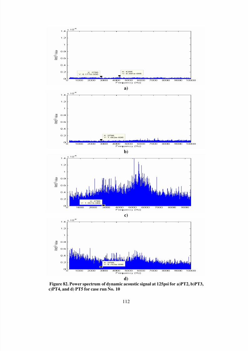
8/6/2019 umi-umd-3786
http://slidepdf.com/reader/full/umi-umd-3786 128/146
112
a)
b)
c)
d)Figure 82. Power spectrum of dynamic acoustic signal at 125psi for a)PT2, b)PT3,
c)PT4, and d) PT5 for case run No. 10

8/6/2019 umi-umd-3786
http://slidepdf.com/reader/full/umi-umd-3786 129/146
113
Figure 83. Power spectrum analysis at individual pressure transducers for stagnation pressure 95psi
Figure 84. Power spectrum analysis at individual pressure transducers for stagnation pressure 105psi
CombustorIsolator
Ho
PT1
PT2PT3PT4PT5
CombustorIsolator
AcousticSource
Ho
PT1
PT2PT3PT4PT5
CombustorIsolator
AcousticSource
CombustorIsolator
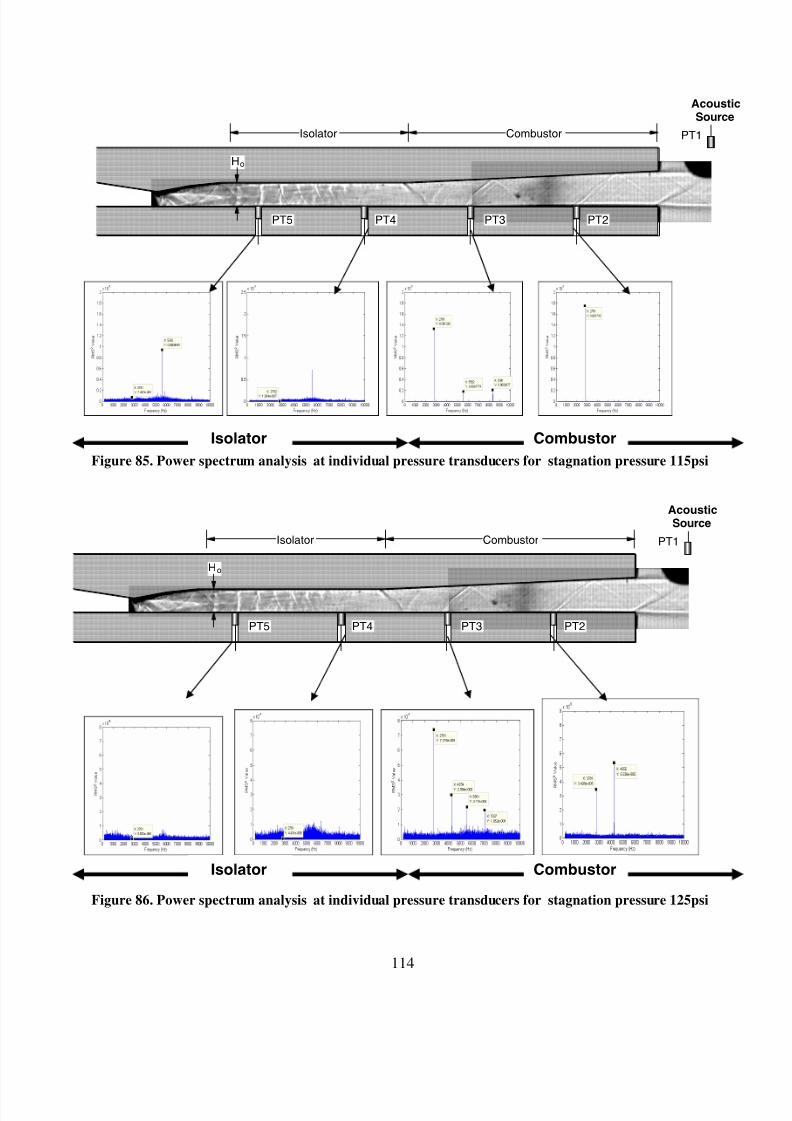
8/6/2019 umi-umd-3786
http://slidepdf.com/reader/full/umi-umd-3786 130/146
114
Figure 85. Power spectrum analysis at individual pressure transducers for stagnation pressure 115psi
Figure 86. Power spectrum analysis at individual pressure transducers for stagnation pressure 125psi
Ho
PT1
PT2PT3PT4PT5
CombustorIsolator
AcousticSource
CombustorIsolator
CombustorIsolator
Ho
PT1
PT2PT3PT4PT5
CombustorIsolator
AcousticSource

8/6/2019 umi-umd-3786
http://slidepdf.com/reader/full/umi-umd-3786 131/146
115
Table 1. Error analysis Values for ratio of dynamic pressure to static pressure
ErrorAnalysis 80psig
Press_Trnsd x(in) Static Dynamic %error_static %error_dyn ratio_dyn_stc %err_Quot Error_Quot
PT2 1.305 1.845 0.01034 0.009230352 0.22244 0.005604336 0.2226286 0.0012477
PT3 3.005 1.0811 0.00623 0.015752474 0.36918 0.005762649 0.3695173 0.0021294
PT4 4.705 17.938 0.002275 0.000949381 1.01099 0.000126826 1.0109895 0.0001282
PT5 6.405 10.784 0.00499 0.001579191 0.46092 0.000462723 0.4609245 0.0002133
90psig
Press_Trnsd x(in) Static Dynamic %error_static %error_dyn ratio_dyn_stc %err_Quot Error_Quot
PT2 1.305 2.982 0.00115 0.005667337 0.429565217 0.000385647 0.4296026 0.0001657
PT3 3.005 1.357 0.00107 0.012225497 0.461682243 0.000788504 0.4618441 0.0003642
PT4 4.705 20.844 0.000055 0.000887066 8.981818182 2.63865E-06 8.9818182 2.37E-05
PT5 6.405 12.611 0.000064 0.001035287 7.71875 5.07493E-06 7.7187501 3.917E-05
100psig
Press_Trnsd x(in) Static Dynamic %error_static %error_dyn ratio_dyn_stc %err_Quot Error_Quot
PT2 1.305 4.224 0.00113 0.004034091 0.401238938 0.000267519 0.4012592 0.0001073
PT3 3.005 1.716 0.0008 0.009545455 0.400125 0.0004662 0.4002388 0.0001866
PT4 4.705 24.277 0.000016 0.00074931 0.85625 6.5906E-07 0.8562503 5.643E-07
PT5 6.405 15.827 0.000047 0.000796108 0.59787234 2.96961E-06 0.5978729 1.775E-06
110psig
Press_Trnsd x(in) Static DYN %error_static %error_dyn rat_dyn_st %err_Quot Error_Quot
PT2 1.305 5.247 0.0000154 0.003329522 0.922077922 2.93501E-06 0.9220839 2.706E-06
PT3 3.005 2.013 0.0000206 0.007908594 0.799514563 1.02335E-05 0.7995537 8.182E-06
PT4 4.705 27.607 0.000009 0.000532474 1.488888889 3.26004E-07 1.488889 4.854E-07
PT5 6.405 19.184 0.000011 0.000802752 0.727272727 5.73394E-07 0.7272732 4.17E-07

8/6/2019 umi-umd-3786
http://slidepdf.com/reader/full/umi-umd-3786 132/146

8/6/2019 umi-umd-3786
http://slidepdf.com/reader/full/umi-umd-3786 133/146
117
Table 4. Phase analysis w.r.t upstream stagnation pressure of 115psi
Po=100psig
Dom_freq(Hz) 4.2kHz run1 run2 run3 run4 run5 run6 run7 run8 run9 run10
x_positon phase_deg phase deg phase_deg phase deg phase_deg phase deg phase_deg phase deg phase_deg phase deg
PT2_phase(deg) 1.305 2.07 72.48 -177.30 86.58 38.70 -24.54 57.41 139.04 -16.74 26.51
PT3_phase(deg) 3.005 -33.02 33.39 148.53 52.79 5.08 -63.28 18.13 99.85 -52.23 -14.73
PT4_phase(deg) 4.705 105.76 -71.00 -31.98 -151.48 116.09 162.81 161.06 -90.84 -76.17 73.74
PT5_phase(deg) 6.405 37.03 -19.86 115.19 7.78 -49.43 -144.16 6.58 80.89 -95.74 -50.96
phase_diff phase_diff phase_diff phase_diff phase_diff phase_diff phase_diff phase_diff phase_diff phase_diff
PT2_PT2 1.305 0.00 0.00 0.00 0.00 0.00 0.00 0.00 0.00 0.00 0.00
PT3_PT2 3.005 -35.09 -39.09 -34.18 -33.79 -33.62 -38.74 -39.28 -39.19 -35.50 -41.24
PT4_PT2 4.705 103.69 -143.47 145.31 121.94 77.40 -172.65 103.65 130.12 -59.43 47.23
PT5_PT2 6.405 34.96 -92.34 -67.52 -78.80 -88.12 -119.62 -50.83 -58.15 -79.00 -77.47
Table 5. Phase analysis w.r.t upstream stagnation pressure of 125psi
Po=110psig
Dom_freq(Hz) 4.2kHz run1 run2 run3 run4 run5 run6 run7 run8 run9 run10
x_positon phase_deg phase deg phase_deg phase deg phase_deg phase deg phase_deg phase deg phase_deg phase deg
PT2_phase(deg) 1.305 -67.35 -151.64 113.81 95.64 73.11 -56.81 72.43 179.52 143.66 -155.24
PT3_phase(deg) 3.005 -100.53 163.07 70.98 53.29 20.20 -110.54 15.94 127.79 98.07 147.27
PT4_phase(deg) 4.705 -149.54 16.57 -78.40 -120.31 172.13 63.50 -149.25 -127.88 -117.06 26.52
PT5_phase(deg) 6.405 -27.55 153.65 137.96 51.54 13.94 -91.66 54.20 117.72 147.57 -168.49
phase_diff phase_diff phase_diff phase_diff phase_diff phase_diff phase_diff phase_diff phase_diff phase_diff
PT2_PT2 1.305 0.00 0.00 0.00 0.00 0.00 0.00 0.00 0.00 0.00 0.00
PT3_PT2 3.005 -33.18 -45.29 -42.84 -42.35 -52.92 -53.73 -56.49 -51.73 -45.59 -57.50
PT4_PT2 4.705 -82.19 168.20 167.78 144.05 99.01 120.31 138.32 52.61 99.28 -178.24
PT5_PT2 6.405 39.80 -54.71 24.15 -44.10 -59.17 -34.85 -18.23 -61.80 3.91 -13.26

8/6/2019 umi-umd-3786
http://slidepdf.com/reader/full/umi-umd-3786 134/146
118
Table 6. Static pressure at each pressure transducer location w.r.t upstream stagnation pressure of
80psig
80psig Upstream(psig) pt2(psig) pt3(psig) pt4(psig) pt5(psig)
80.23 1.83 1.08 17.93 10.77
80.25 1.86 1.10 17.94 10.77
80.25 1.83 1.09 17.93 10.77
80.18 1.88 1.10 17.91 10.77
80.23 1.87 1.09 17.92 10.76
80.23 1.85 1.09 17.93 10.77
80.22 1.82 1.10 17.93 10.77
80.23 1.84 1.09 17.93 10.77
80.22 1.86 1.05 17.93 10.80
80.21 1.84 1.07 17.94 10.79
80.16 1.83 1.10 17.94 10.76
80.17 1.82 1.07 17.96 10.76
80.19 1.85 1.08 17.93 10.76
80.18 1.85 1.10 17.90 10.78
80.15 1.86 1.12 17.93 10.79
80.15 1.85 1.08 17.93 10.78
80.16 1.88 1.08 17.92 10.76
80.11 1.88 1.08 17.90 10.79
80.15 1.85 1.07 17.93 10.79
80.18 1.85 1.05 17.94 10.77
80.16 1.86 1.07 17.93 10.80
80.12 1.85 1.10 17.93 10.79
80.10 1.85 1.09 17.97 10.77
80.12 1.85 1.07 17.95 10.80
80.12 1.85 1.08 17.94 10.79
80.16 1.85 1.12 17.93 10.79
80.09 1.88 1.11 17.95 10.79
80.09 1.84 1.09 17.93 10.78
80.08 1.85 1.09 17.93 10.76
80.15 1.84 1.07 17.95 10.77
80.12 1.84 1.05 17.93 10.79
80.11 1.82 1.08 17.92 10.78
80.15 1.85 1.09 17.95 10.82
80.16 1.84 1.08 17.94 10.81
80.12 1.83 1.06 17.96 10.76
80.12 1.82 1.07 17.97 10.80
80.13 1.83 1.07 17.96 10.81
80.09 1.85 1.10 17.93 10.77
80.13 1.86 1.09 17.93 10.79
80.14 1.87 1.09 17.92 10.80
80.16 1.86 1.08 17.93 10.78
80.18 1.85 1.04 17.93 10.80
80.14 1.83 1.07 17.93 10.78
80.18 1.85 1.07 17.94 10.80
80.19 1.85 1.07 17.94 10.81
80.15 1.84 1.07 17.91 10.82

8/6/2019 umi-umd-3786
http://slidepdf.com/reader/full/umi-umd-3786 135/146
119
80.15 1.85 1.06 17.96 10.79
80.21 1.84 1.08 17.95 10.79
80.13 1.85 1.08 17.93 10.79
80.19 1.85 1.11 17.93 10.79
80.20 1.84 1.08 17.93 10.79
80.19 1.85 1.09 17.93 10.79
80.23 1.87 1.06 17.94 10.77
80.22 1.88 1.08 17.93 10.79
80.19 1.85 1.06 17.94 10.79
80.25 1.84 1.07 17.95 10.80
80.23 1.83 1.08 17.95 10.81
80.22 1.86 1.09 17.93 10.79
80.19 1.85 1.07 17.96 10.79
80.20 1.84 1.09 17.95 10.79
80.18 1.81 1.07 17.93 10.79
80.25 1.83 1.11 17.93 10.79
80.16 1.84 1.08 17.93 10.79
80.16 1.87 1.09 17.94 10.79
80.22 1.86 1.07 17.92 10.76
80.20 1.83 1.09 17.93 10.78
80.20 1.81 1.07 17.93 10.79
80.24 1.86 1.08 17.93 10.79
80.19 1.83 1.06 17.95 10.80
80.22 1.83 1.07 17.93 10.79
80.20 1.85 1.08 17.96 10.77
80.19 1.82 1.06 17.95 10.79
80.17 1.86 1.10 17.94 10.77
80.22 1.86 1.08 17.93 10.78
80.22 1.82 1.10 17.93 10.79
80.19 1.87 1.07 17.93 10.79
80.17 1.84 1.07 17.92 10.78
80.24 1.86 1.06 17.96 10.79
80.19 1.83 1.08 17.94 10.78
80.15 1.82 1.06 17.94 10.79
80.17 1.84 1.07 17.95 10.79
80.16 1.86 1.08 17.93 10.78
80.11 1.88 1.07 17.96 10.78
80.19 1.85 1.10 17.96 10.79
80.17 1.85 1.09 17.94 10.78
80.16 1.85 1.09 17.93 10.78
Avg 80.17 1.85 1.08 17.94 10.78
STDV 0.04 0.02 0.01 0.01 0.01
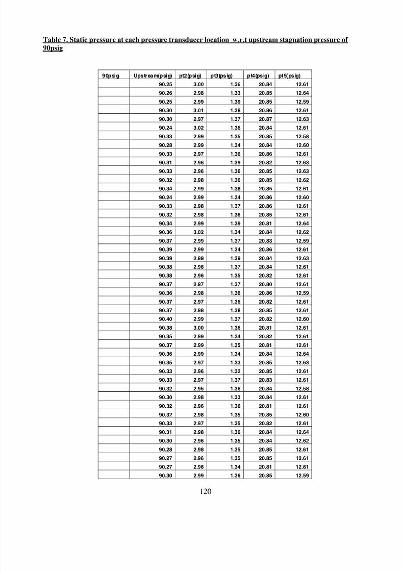
8/6/2019 umi-umd-3786
http://slidepdf.com/reader/full/umi-umd-3786 136/146
120
Table 7. Static pressure at each pressure transducer location w.r.t upstream stagnation pressure of
90psig
90psig Upstream(psig) pt2(psig) pt3(psig) pt4(psig) pt5(psig)
90.25 3.00 1.36 20.84 12.61
90.26 2.98 1.33 20.85 12.64
90.25 2.99 1.39 20.85 12.59
90.30 3.01 1.38 20.86 12.61
90.30 2.97 1.37 20.87 12.63
90.24 3.02 1.36 20.84 12.61
90.33 2.99 1.35 20.85 12.58
90.28 2.99 1.34 20.84 12.60
90.33 2.97 1.36 20.86 12.61
90.31 2.96 1.39 20.82 12.63
90.33 2.96 1.36 20.85 12.63
90.32 2.98 1.36 20.85 12.62
90.34 2.99 1.38 20.85 12.61
90.24 2.99 1.34 20.86 12.60
90.33 2.98 1.37 20.86 12.61
90.32 2.98 1.36 20.85 12.61
90.34 2.99 1.39 20.81 12.64
90.36 3.02 1.34 20.84 12.62
90.37 2.99 1.37 20.83 12.59
90.39 2.99 1.34 20.86 12.61
90.39 2.99 1.39 20.84 12.63
90.38 2.96 1.37 20.84 12.61
90.38 2.96 1.35 20.82 12.61
90.37 2.97 1.37 20.80 12.61
90.36 2.98 1.36 20.86 12.59
90.37 2.97 1.36 20.82 12.61
90.37 2.98 1.38 20.85 12.61
90.40 2.99 1.37 20.82 12.60
90.38 3.00 1.36 20.81 12.61
90.35 2.99 1.34 20.82 12.61
90.37 2.99 1.35 20.81 12.61
90.36 2.99 1.34 20.84 12.64
90.35 2.97 1.33 20.85 12.63
90.33 2.96 1.32 20.85 12.61
90.33 2.97 1.37 20.83 12.61
90.32 2.95 1.36 20.84 12.58
90.30 2.98 1.33 20.84 12.61
90.32 2.96 1.36 20.81 12.61
90.32 2.98 1.35 20.85 12.60
90.33 2.97 1.35 20.82 12.61
90.31 2.98 1.36 20.84 12.64
90.30 2.96 1.35 20.84 12.62
90.28 2.98 1.35 20.85 12.61
90.27 2.96 1.35 20.85 12.61
90.27 2.96 1.34 20.81 12.61
90.30 2.99 1.36 20.85 12.59
8/6/2019 umi-umd-3786
http://slidepdf.com/reader/full/umi-umd-3786 137/146
121
90.28 2.96 1.39 20.85 12.61
90.27 2.96 1.39 20.85 12.60
90.26 2.99 1.36 20.85 12.61
90.25 3.00 1.34 20.85 12.59
90.22 2.96 1.36 20.86 12.61
90.28 3.00 1.37 20.82 12.60
90.24 2.99 1.35 20.84 12.61
90.22 2.99 1.33 20.84 12.62
90.21 2.97 1.32 20.85 12.61
90.19 3.01 1.34 20.86 12.61
90.23 2.97 1.36 20.85 12.60
90.17 2.97 1.36 20.85 12.60
90.20 2.97 1.36 20.81 12.61
90.24 2.97 1.36 20.83 12.63
90.20 2.99 1.35 20.85 12.59
90.15 2.99 1.36 20.88 12.61
90.22 2.95 1.37 20.86 12.61
90.24 2.96 1.36 20.83 12.63
90.15 2.96 1.36 20.83 12.61
90.18 2.99 1.33 20.81 12.63
90.20 2.99 1.37 20.89 12.61
90.24 2.97 1.36 20.85 12.62
90.20 2.97 1.35 20.86 12.61
90.21 2.99 1.36 20.87 12.62
90.24 3.00 1.38 20.86 12.61
90.21 2.99 1.36 20.85 12.62
90.19 2.99 1.34 20.83 12.61
90.19 2.99 1.35 20.85 12.61
90.23 2.96 1.36 20.85 12.61
90.24 3.00 1.35 20.85 12.61
90.25 2.98 1.33 20.85 12.63
90.27 2.99 1.36 20.85 12.63
90.25 2.97 1.36 20.85 12.59
90.26 3.01 1.35 20.84 12.62
90.24 3.01 1.36 20.88 12.61
90.25 2.96 1.35 20.85 12.61
90.27 2.98 1.38 20.87 12.63
90.26 3.00 1.39 20.86 12.64
90.24 3.02 1.37 20.86 12.60
90.21 3.00 1.37 20.86 12.61
Avg 90.28 2.98 1.36 20.84 12.61
STDV 0.06 0.02 0.02 0.02 0.01
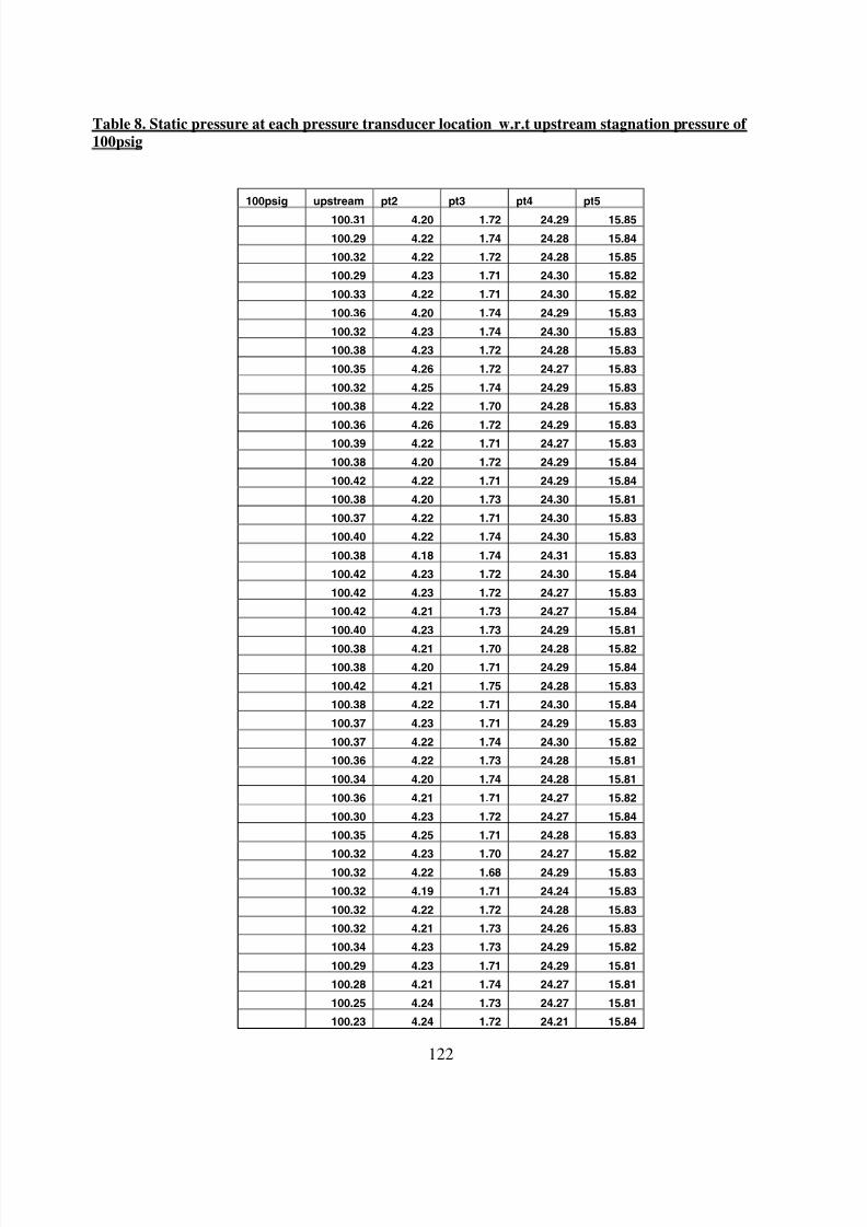
8/6/2019 umi-umd-3786
http://slidepdf.com/reader/full/umi-umd-3786 138/146
122
Table 8. Static pressure at each pressure transducer location w.r.t upstream stagnation pressure of
100psig
100psig upstream pt2 pt3 pt4 pt5
100.31 4.20 1.72 24.29 15.85
100.29 4.22 1.74 24.28 15.84
100.32 4.22 1.72 24.28 15.85
100.29 4.23 1.71 24.30 15.82
100.33 4.22 1.71 24.30 15.82
100.36 4.20 1.74 24.29 15.83
100.32 4.23 1.74 24.30 15.83
100.38 4.23 1.72 24.28 15.83
100.35 4.26 1.72 24.27 15.83
100.32 4.25 1.74 24.29 15.83
100.38 4.22 1.70 24.28 15.83
100.36 4.26 1.72 24.29 15.83100.39 4.22 1.71 24.27 15.83
100.38 4.20 1.72 24.29 15.84
100.42 4.22 1.71 24.29 15.84
100.38 4.20 1.73 24.30 15.81
100.37 4.22 1.71 24.30 15.83
100.40 4.22 1.74 24.30 15.83
100.38 4.18 1.74 24.31 15.83
100.42 4.23 1.72 24.30 15.84
100.42 4.23 1.72 24.27 15.83
100.42 4.21 1.73 24.27 15.84
100.40 4.23 1.73 24.29 15.81
100.38 4.21 1.70 24.28 15.82
100.38 4.20 1.71 24.29 15.84
100.42 4.21 1.75 24.28 15.83
100.38 4.22 1.71 24.30 15.84
100.37 4.23 1.71 24.29 15.83
100.37 4.22 1.74 24.30 15.82
100.36 4.22 1.73 24.28 15.81
100.34 4.20 1.74 24.28 15.81
100.36 4.21 1.71 24.27 15.82
100.30 4.23 1.72 24.27 15.84
100.35 4.25 1.71 24.28 15.83
100.32 4.23 1.70 24.27 15.82
100.32 4.22 1.68 24.29 15.83
100.32 4.19 1.71 24.24 15.83
100.32 4.22 1.72 24.28 15.83
100.32 4.21 1.73 24.26 15.83
100.34 4.23 1.73 24.29 15.82
100.29 4.23 1.71 24.29 15.81
100.28 4.21 1.74 24.27 15.81
100.25 4.24 1.73 24.27 15.81
100.23 4.24 1.72 24.21 15.84

8/6/2019 umi-umd-3786
http://slidepdf.com/reader/full/umi-umd-3786 139/146
123
100.22 4.23 1.73 24.28 15.82
100.21 4.23 1.71 24.24 15.83
100.19 4.23 1.67 24.29 15.84
100.22 4.23 1.69 24.28 15.83
100.20 4.23 1.71 24.27 15.82
100.16 4.18 1.72 24.27 15.85
100.16 4.26 1.72 24.24 15.80
100.12 4.24 1.71 24.28 15.82
100.12 4.21 1.74 24.27 15.80
100.13 4.24 1.72 24.27 15.83
100.15 4.26 1.71 24.29 15.81
100.13 4.23 1.73 24.27 15.81
100.13 4.23 1.73 24.26 15.82
100.11 4.22 1.71 24.23 15.83
100.12 4.23 1.72 24.28 15.83
100.13 4.20 1.69 24.27 15.83
100.14 4.23 1.69 24.28 15.82
100.11 4.22 1.74 24.29 15.80
100.13 4.23 1.69 24.28 15.80
100.10 4.23 1.71 24.27 15.82
100.15 4.23 1.73 24.24 15.81
100.15 4.23 1.71 24.27 15.80
100.13 4.26 1.71 24.30 15.81
100.18 4.25 1.69 24.27 15.83
100.20 4.23 1.71 24.27 15.84
100.16 4.22 1.70 24.29 15.83
100.14 4.23 1.71 24.30 15.83
100.19 4.23 1.70 24.25 15.83
100.19 4.21 1.74 24.26 15.83
100.20 4.23 1.73 24.28 15.83
100.17 4.23 1.72 24.26 15.82
100.21 4.26 1.74 24.28 15.83
100.23 4.24 1.73 24.28 15.81
100.26 4.21 1.70 24.27 15.83
100.31 4.23 1.69 24.26 15.84
100.30 4.24 1.73 24.26 15.84
100.28 4.26 1.71 24.27 15.84
100.32 4.22 1.71 24.28 15.86
100.33 4.20 1.68 24.26 15.85
100.32 4.23 1.70 24.29 15.84
100.31 4.21 1.73 24.28 15.83
100.35 4.22 1.74 24.25 15.82
100.27 4.22 1.72 24.28 15.83
0.10 0.02 0.02 0.02 0.01
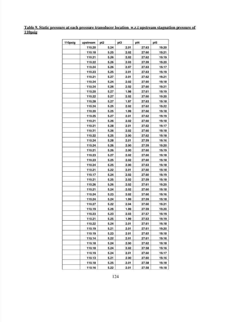
8/6/2019 umi-umd-3786
http://slidepdf.com/reader/full/umi-umd-3786 140/146
124
Table 9. Static pressure at each pressure transducer location w.r.t upstream stagnation pressure of
110psig
110psig upstream pt2 pt3 pt4 pt5
110.20 5.24 2.01 27.63 19.20
110.18 5.25 2.02 27.60 19.21
110.21 5.26 2.02 27.62 19.19
110.22 5.26 2.03 27.59 19.20
110.24 5.26 2.07 27.63 19.17
110.23 5.25 2.01 27.63 19.19
110.21 5.27 2.01 27.62 19.21
110.24 5.24 2.02 27.60 19.18
110.24 5.26 2.02 27.60 19.21
110.20 5.27 1.98 27.61 19.19
110.22 5.27 2.02 27.60 19.20
110.28 5.27 1.97 27.63 19.18
110.24 5.25 2.02 27.62 19.22
110.20 5.25 1.99 27.60 19.18
110.25 5.27 2.01 27.62 19.19
110.21 5.26 2.02 27.60 19.18
110.21 5.28 2.01 27.62 19.17
110.21 5.26 2.02 27.60 19.18
110.22 5.25 2.00 27.62 19.18
110.24 5.28 2.01 27.59 19.16
110.24 5.26 2.00 27.59 19.20
110.21 5.26 2.00 27.60 19.19
110.23 5.27 2.02 27.60 19.18
110.23 5.25 2.02 27.60 19.18
110.24 5.25 2.00 27.63 19.18
110.21 5.22 2.01 27.60 19.18
110.17 5.24 2.02 27.60 19.19
110.21 5.25 2.02 27.59 19.18
110.26 5.26 2.02 27.61 19.20
110.21 5.24 2.02 27.60 19.18
110.24 5.23 2.02 27.60 19.16
110.24 5.24 1.99 27.59 19.18
110.27 5.22 2.04 27.60 19.21
110.19 5.26 1.99 27.59 19.20
110.23 5.23 2.03 27.57 19.19
110.21 5.25 1.99 27.63 19.19
110.22 5.24 2.01 27.61 19.18
110.19 5.21 2.01 27.61 19.20
110.19 5.23 2.01 27.62 19.18
110.14 5.22 2.01 27.61 19.16
110.18 5.24 2.00 27.62 19.18
110.18 5.24 2.02 27.58 19.16
110.19 5.24 2.01 27.60 19.17
110.13 5.21 2.00 27.60 19.16
110.18 5.25 2.01 27.58 19.18
110.16 5.22 2.01 27.58 19.18

8/6/2019 umi-umd-3786
http://slidepdf.com/reader/full/umi-umd-3786 141/146
125
110.18 5.24 2.02 27.62 19.17
110.15 5.26 1.99 27.63 19.18
110.15 5.19 2.00 27.61 19.19
110.15 5.25 2.03 27.60 19.17
110.13 5.24 2.03 27.61 19.17
110.15 5.25 2.02 27.59 19.18
110.12 5.25 2.02 27.60 19.18
110.11 5.26 1.99 27.60 19.15
110.16 5.27 2.01 27.60 19.15
110.11 5.27 2.01 27.60 19.18
110.15 5.27 2.00 27.60 19.19
110.14 5.27 2.00 27.60 19.18
110.11 5.26 2.00 27.60 19.16
110.11 5.26 2.01 27.62 19.17
110.08 5.27 2.02 27.62 19.19
110.10 5.24 2.02 27.62 19.18
110.10 5.25 2.02 27.62 19.16
110.10 5.25 2.02 27.60 19.19
110.07 5.27 1.99 27.62 19.17
110.09 5.26 2.00 27.60 19.15
110.12 5.24 2.03 27.60 19.18
110.08 5.24 2.00 27.60 19.18
110.14 5.24 2.01 27.61 19.19
110.15 5.27 2.00 27.59 19.20
110.15 5.25 1.99 27.63 19.19
110.15 5.24 2.01 27.64 19.18
110.12 5.24 2.00 27.61 19.19
110.14 5.21 2.02 27.62 19.21
110.18 5.25 2.05 27.62 19.19
110.18 5.24 2.00 27.61 19.18
110.20 5.25 2.04 27.61 19.18
110.16 5.25 2.03 27.60 19.15
110.20 5.22 2.01 27.62 19.20
110.21 5.24 2.01 27.57 19.22
110.20 5.24 2.01 27.61 19.20
110.18 5.24 2.00 27.60 19.19
110.21 5.25 1.99 27.62 19.19
110.16 5.23 2.02 27.63 19.18
110.20 5.22 2.03 27.63 19.20
110.23 5.23 2.05 27.62 19.19
110.18 5.25 2.01 27.61 19.18
0.05 0.02 0.02 0.01 0.02
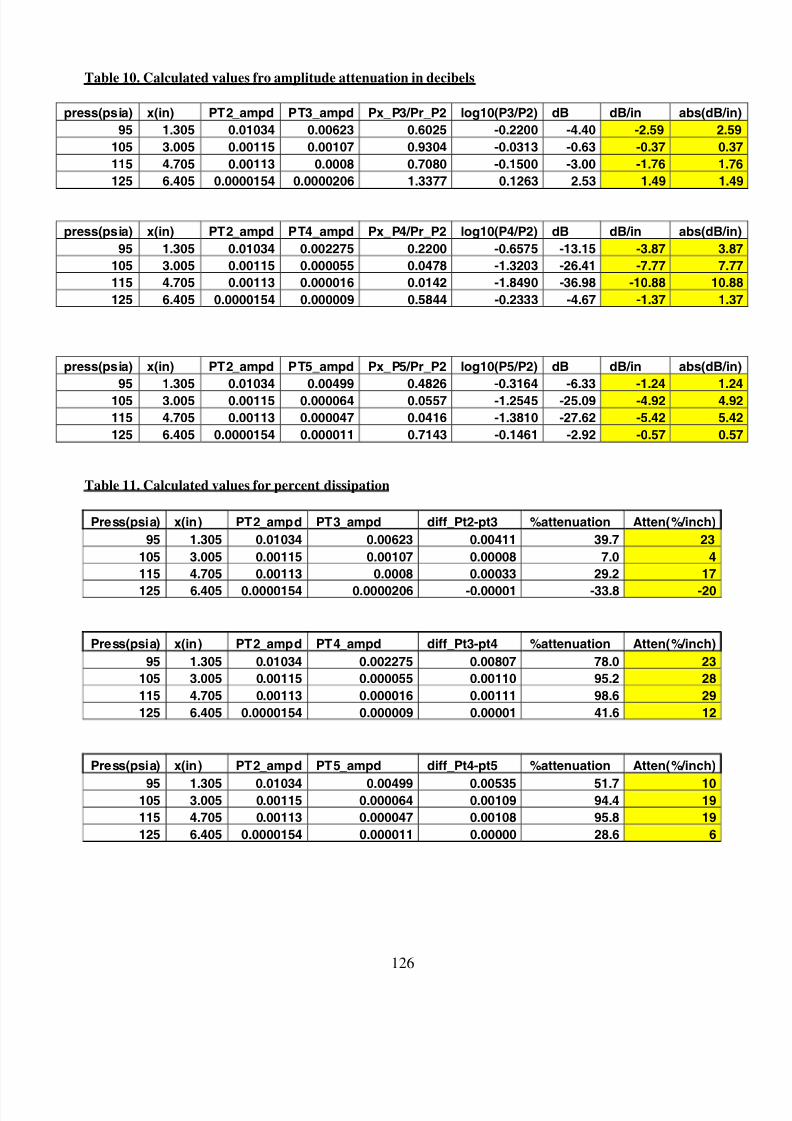
8/6/2019 umi-umd-3786
http://slidepdf.com/reader/full/umi-umd-3786 142/146
126
Table 10. Calculated values fro amplitude attenuation in decibels
press(psia) x(in) PT2_ampd PT3_ampd Px_P3/Pr_P2 log10(P3/P2) dB dB/in abs(dB/in)
95 1.305 0.01034 0.00623 0.6025 -0.2200 -4.40 -2.59 2.59
105 3.005 0.00115 0.00107 0.9304 -0.0313 -0.63 -0.37 0.37
115 4.705 0.00113 0.0008 0.7080 -0.1500 -3.00 -1.76 1.76
125 6.405 0.0000154 0.0000206 1.3377 0.1263 2.53 1.49 1.49
press(psia) x(in) PT2_ampd PT4_ampd Px_P4/Pr_P2 log10(P4/P2) dB dB/in abs(dB/in)
95 1.305 0.01034 0.002275 0.2200 -0.6575 -13.15 -3.87 3.87
105 3.005 0.00115 0.000055 0.0478 -1.3203 -26.41 -7.77 7.77
115 4.705 0.00113 0.000016 0.0142 -1.8490 -36.98 -10.88 10.88
125 6.405 0.0000154 0.000009 0.5844 -0.2333 -4.67 -1.37 1.37
press(psia) x(in) PT2_ampd PT5_ampd Px_P5/Pr_P2 log10(P5/P2) dB dB/in abs(dB/in)
95 1.305 0.01034 0.00499 0.4826 -0.3164 -6.33 -1.24 1.24
105 3.005 0.00115 0.000064 0.0557 -1.2545 -25.09 -4.92 4.92
115 4.705 0.00113 0.000047 0.0416 -1.3810 -27.62 -5.42 5.42
125 6.405 0.0000154 0.000011 0.7143 -0.1461 -2.92 -0.57 0.57
Table 11. Calculated values for percent dissipation
Press(psia) x(in) PT2_ampd PT3_ampd diff_Pt2-pt3 %attenuation Atten(%/inch)
95 1.305 0.01034 0.00623 0.00411 39.7 23
105 3.005 0.00115 0.00107 0.00008 7.0 4
115 4.705 0.00113 0.0008 0.00033 29.2 17
125 6.405 0.0000154 0.0000206 -0.00001 -33.8 -20
Press(psia) x(in) PT2_ampd PT4_ampd diff_Pt3-pt4 %attenuation Atten(%/inch)
95 1.305 0.01034 0.002275 0.00807 78.0 23
105 3.005 0.00115 0.000055 0.00110 95.2 28
115 4.705 0.00113 0.000016 0.00111 98.6 29
125 6.405 0.0000154 0.000009 0.00001 41.6 12
Press(psia) x(in) PT2_ampd PT5_ampd diff_Pt4-pt5 %attenuation Atten(%/inch)
95 1.305 0.01034 0.00499 0.00535 51.7 10105 3.005 0.00115 0.000064 0.00109 94.4 19
115 4.705 0.00113 0.000047 0.00108 95.8 19
125 6.405 0.0000154 0.000011 0.00000 28.6 6

8/6/2019 umi-umd-3786
http://slidepdf.com/reader/full/umi-umd-3786 143/146
127
References
1. Falempin, F.H., “Scramjet Developments in France,” Scramjet Propulsion: Progress in
Astronautics and Aeronautics, Vol.189, pp47, 2000.
2. Curran, Edward T., “Scramjet Engines: The First Forty Years,” Journal of Propulsion
and Power , Vol. 17, No. 6, November-December 2001.
3. Sabel’nikov, V. and Penzin, V.I., “Scramjet Research and Development in Russia,” Scramjet
Propulsion: Progress in Astronautics and Aeronautics, Vol.189, pp223, 2000.
4. Chinzei, N., Mitani, T., Yatsuyanagi, N., “ Scramjet Engine Research at the National
Aerospace Laboratory in Japan,” Scramjet Propulsion: Progress in Astronautics and
Aeronautics, Vol.189, pp160, 2000.
5. Fry, Ronald S., “ A Century of Ramjet Propulsion Technology Evolution,” Journal of
Propulsion
and Power , Vol. 20, No. 1, January-February 2004.
6. Waltrup, Paul J., “Liquid-Fueled Supersonic Combustion Ramjets: A Research Perspective,”
Journal of Propulsion and Power , Vol. 3, No. 6, Nov-Dec 1987.
7. Ma, Fuhua, Li, Juan, and Yang, Vigor,” Thermoacoustic Flow Instability in Scramjet
Combustor,”
AIAA-2005-3824, 41st
AIAA/ASME/SAE/ASEE Joint Propulsion Conference and Exhibit ,
Tucson, Az, July 2005.
8. Andrews, Earl H., “Scramjet Development and Testing in the United States,” AIAA-2001-
1927,
AIAA/NAL-NASADA-ISAS 10th
International Space Planes and Hypersonic Systems and
Technologies Conference, Kyoto, Japan, April 2001.
9. Curran, E.T., Heiser, W.H., Pratt, D.T., “Fluid Phenomena in Scramjet Combustion Systems,”

8/6/2019 umi-umd-3786
http://slidepdf.com/reader/full/umi-umd-3786 144/146
128
Annual Review of Fluid Mechanics, Vol.28, pp 323-360, 1996.
10. Roy, Gabriel D., “Performance Enhancement and Thermo-Acoustic Instability Suppression by
Combustion Control,” A01-16135, 36 th
AIAA Aerospace Sciences Meeting and Exhibit , Reno,
NV, Jan 2001.
11. Culick, F.E.C., “Dynamic of Combustion Systems: Fundamentals, Acoustics and Control,”
California Institute of Technology”, 2001.
12. Yang, Vigor, “Introductions: Stability Characteristics and Control Approaches,” Von Karman
Institute for Fluid Dynamics,” May 2001.
13. Yu, K., Pang, B., Hsu, O., “Implementing Active Combustion Control in Propulsion Systems,”
37th
AIAA/ASME/SAE/ASEE/ Joint Propulsion Conference and Exhibit, Salt Lake City , Utah
A1AA 2001-3849, July 2001.
14. Yu, K., Wilson, K. J., Schadow, K.C., “Active Combustion Control in a Liquid-Fueled Dump
Combustor,” AIAA 97-0462, 35th
AIAA Aerospace Sciences Meeting and Exhibit , Reno, NV,
Jan 2001.
15. Le, D., DeLaat, J., and Chang, C., “Control of Thermo-Acoustic Instabilities: The Multi-Scale
Kalman Approach,” AIAA-2003-4934, 39TH
AIAA/ASME/SAE/ASEE Joint Propulsion
Conference
and Exhibit , Huntsville, AL, July 2003.
16. Hsu, O., Yu, K., and Wilson, K.J., “Liquid-fueled active combustion control- Effect of Inlet
Flow Temperature,” AIAA-2001-1131, 39TH Aerospace Sciences Meeting and Exhibit, Reno,
NV, Jan 2001.
17. Yi, T., Cornwell, M., Gutmark, E., “Dynamics and Control of a High Frequency Fuel Valve
and its Application to ACTIVE Combustion Control,” AIAA-2004-4034, 40TH

8/6/2019 umi-umd-3786
http://slidepdf.com/reader/full/umi-umd-3786 145/146
129
AIAA/ASME/SAE/ASEE Joint Propulsion Conference and Exhibit , Fort Lauderdale, FL, July
2004.
18. Acharya, S., Murugappan, S., Annaswamy, M., Gutmark, E. J., “Characteristics and Control of
Combustion Instabilities in Swirl-Spray Combustor, ” Journal of Propulsion and Power , Vol.
19, No. 3, 2003.
19. Hathout, J. P., Fleifill, M., Annaswamy, M., Ghoniem, A. f., “Combustion Instability Active
Control Using Periodic Fuel Injection,” Journal of Propulsion and Power , Vol. 18, No. 2,
2002.
20. Marrot, F., Gajan, P., Pauzin, S., Simon, F., “Experimental Application of an Active Control
Loop on Backward-Facing Step Flow,” AIAA Journal, Vol.43, No.6, 2005.
21. Menon, S., “Numerical Simulation and Active Control of Combustion Instability in a
Ramjet Combustor,” AIAA-90-3930, AIAA 13TH
Aeroacoustics Conference, Tallahassee, FL,
Oct. 1990.
22. Raman, Ganesh, “Advances in Understanding Supersonic Jet Screech,”AIAA- 98-0279
36 th
AIAA Aerospace Sciences Meeting and Exhibit , Reno NV, 2000.
23. Salikuddin, M., Tam, C.K., Burrin, R.H, Gallegher, J.A., “An Experimental and Theoretical
Investigation of the propagation of Sound Waves Through a Turbulent Boundary Layer,”
Journal Sound and Vibration 127(1) p. 91-127, 1988.
24. Anderson, J.D, Modern Compressible Flow with Historical Perspective, McGraw Hill ,
pp.132, 2003.
25. Shapiro, A. H., The Dynamics and Thermodynamics of Compressible Fluid Flow, The
Ronald Press Company, NY, Vol.1, pp.55, 1953.
26. Aksel, M. Haluk and Eralp, O. Cahit, Gas Dynamics, Prentice Hall International, Great
Britain, pp73, 1994.

8/6/2019 umi-umd-3786
http://slidepdf.com/reader/full/umi-umd-3786 146/146
27. Hausmann, Erich, and Slack, Edgar P., Physics 2nd
Ed., D. Van Nostrand Company, Inc.
NY, pp553-554, 1939.
28. Gough, W., Richards, J.P.G., AND Williams, R.P., Vibrations and Waves 2nd
Ed., Prentice
Hall International, Great Britain, pp182-187, 1996.
29. Speaks, Charles E., Introduction to Sound: Acoustics for the Hearing and Speech Science,
3rd
Ed., Singular Publishing Group, Inc., CA, pp271-275, 1999.
30. Anderson Jr., J.D, Fundamentals of Aerodynamics, McGraw Hill , NY, pp. 517-539, 1984.
31. Shapiro, A. H., The Dynamics and Thermodynamics of Compressible Fluid Flow, The
Ronald Press Company, NY, Vol.2, 1953.
32. Anderson Jr., J.D, Hypersonic And High Temperature Gasdynamics, AIAA Inc. , pp224-225,
1989.
33. Houghton, E.L., Carpenter, P.W., Aerodynamics for Engineering Students 5th
Ed.,
Butterworth and Heinemann, pp375-481, 2003.


![[3786] – 21](https://img.dokumen.tips/doc/110x75/61da88ea91fbc310454c9d37/3786-21.jpg)


