UMAP 2001 vol. 22 No. 3

7/17/2019 UMAP 2001 vol. 22 No. 3

http://slidepdf.com/reader/full/umap-2001-vol-22-no-3 1/164

The

UMAPJournal

PublisherCOMAP, Inc.

Vol. 22, No. 3Executive PublisherSolomon A. Garfunkel

ILAP EditorDavid C. “Chris” ArneyDean of the School of

Mathematics and SciencesThe College of Saint Rose

432 Western AvenueAlbany, NY [email protected]

On Jargon EditorYves NievergeltDepartment of MathematicsEastern Washington UniversityCheney, WA [email protected]

Reviews Editor James M. CargalP.O. Box 210667Montgomery, AL 36121–[email protected]

Development DirectorLaurie W. Aragon

Production ManagerGeorge W. Ward

Project ManagerRoland Cheyney

Copy EditorsSeth A. MaislinPauline Wright

Distribution ManagerKevin Darcy

Production SecretaryGail Wessell

Graphic DesignerDaiva Kiliulis

Editor

Paul J. CampbellCampus Box 194Beloit College700 College St.Beloit, WI 53511–[email protected]

Associate Editors

Don AdolphsonDavid C. “Chris” ArneyRon BarnesArthur Benjamin

James M. CargalMurray K. ClaytonCourtney S. ColemanLinda L. Deneen

James P. Fink Solomon A. GarfunkelWilliam B. GearhartWilliam C. GiauqueRichard HabermanCharles E. LienertWalter MeyerYves Nievergelt

John S. RobertsonGarry H. RodrigueNed W. SchillowPhilip D. Straf Þn

J.T. SutcliffeDonna M. SzottGerald D. TaylorMaynard ThompsonKen TraversRobert E.D. “Gene” Woolsey

Brigham Young UniversityThe College of St. RoseUniversity of Houston—DowntownHarvey Mudd College

Troy State University MontgomeryUniversity of Wisconsin—MadisonHarvey Mudd CollegeUniversity of Minnesota, DuluthGettysburg CollegeCOMAP, Inc.California State University, FullertoBrigham Young UniversitySouthern Methodist UniversityMetropolitan State CollegeAdelphi UniversityEastern Washington UniversityGeorgia College and State UniversiLawrence Livermore LaboratoryLehigh Carbon Community CollegeBeloit College

St. Mark’s School, DallasComm. College of Allegheny CounColorado State UniversityIndiana UniversityUniversity of IllinoisColorado School of Mines

7/17/2019 UMAP 2001 vol. 22 No. 3


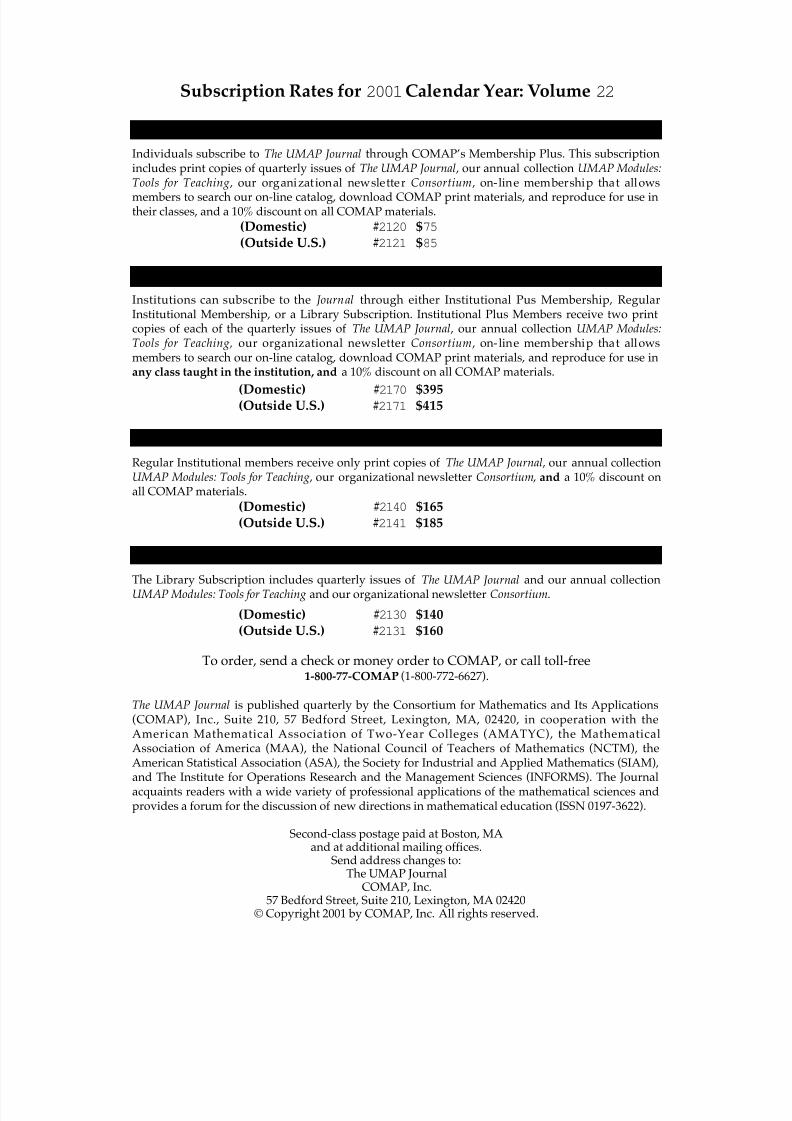
Subscription Rates for 2001 Calendar Year: Volume 22

Individuals subscribe to The UMAP Journal through COMAP’s Membership Plus. This subscriptionincludes print copies of quarterly issues of The UMAP Journal , our annual collection UMAP Modules:Tools for Teaching , our organizational newsletter Consortium , on-line membership that allows

members to search our on-line catalog, download COMAP print materials, and reproduce for use intheir classes, and a 10% discount on all COMAP materials.

(Domestic) #2120 $75

(Outside U.S.) #2121 $85

Institutions can subscribe to the Journal through either Institutional Pus Membership, RegularInstitutional Membership, or a Library Subscription. Institutional Plus Members receive two printcopies of each of the quarterly issues of The UMAP Journal , our annual collection UMAP Modules:Tools for Teaching, our organizational newsletter Consortium , on- line membership that allowsmembers to search our on-line catalog, download COMAP print materials, and reproduce for use inany class taught in the institution, and a 10% discount on all COMAP materials.

(Domestic) #2170 $395(Outside U.S.) #2171 $415

Regular Institutional members receive only print copies of The UMAP Journal , our annual collectionUMAP Modules: Tools for Teaching , our organizational newsletter Consortium , and a 10% discount onall COMAP materials.


The Library Subscription includes quarterly issues of The UMAP Journal and our annual collectionUMAP Modules: Tools for Teaching and our organizational newsletter Consortium.


To order, send a check or money order to COMAP, or call toll-free1-800-77-COMAP (1-800-772-6627).

The UMAP Journal is published quarterly by the Consortium for Mathematics and Its Applications(COMAP), Inc., Suite 210, 57 Bedford Street, Lexington, MA, 02420, in cooperation with theAmerican Mathematical Association of Two-Year Colleges (AMATYC), the MathematicalAssociation of America (MAA), the National Council of Teachers of Mathematics (NCTM), theAmerican Statistical Association (ASA), the Society for Industrial and Applied Mathematics (SIAM),and The Institute for Operations Research and the Management Sciences (INFORMS). The Journalacquaints readers with a wide variety of professional applications of the mathematical sciences andprovides a forum for the discussion of new directions in mathematical education (ISSN 0197-3622).

Second-class postage paid at Boston, MAand at additional mailing offices.

Send address changes to:The UMAP Journal

COMAP, Inc.57 Bedford Street, Suite 210, Lexington, MA 02420

© Copyright 2001 by COMAP, Inc. All rights reserved.

MEMBERSHIP PLUS FOR INDIVIDUAL SUBSCRIBERS

INSTITUTIONAL PLUS MEMBERSHIP SUBSCRIBERS

LIBRARY SUBSCRIPTIONS

INSTITUTIONAL MEMBERSHIP SUBSCRIBERS

7/17/2019 UMAP 2001 vol. 22 No. 3


Vol. 22, No. 3 2001

Table of Contents

Publisher's EditorialThe Face of Things to Come

Solomon A. Garfunkel ..................................................................................185

Modeling ForumResults of the 2001 Contest in Mathematical Modeling ....................187

Frank GiordanoSpokes or Discs?

W.D.V. De Wet, D.F. Malan, and C. Mumbeck ................................211

Selection of a Bicycle Wheel TypeNicholas J. Howard, Zachariah R. Miller,and Matthew R. Adams .................................................................................225

A Systematic Technique for Optimal Bicycle Wheel SelectionMichael B. Flynn, Eamonn T. Long, andWilliam Whelan-Curtin ................................................................................241

Author-Judge's Commentary: The Outstanding Bicycle WheelPapersKelly Black ...........................................................................................................253

Project H.E.R.O.: Hurricane Emergency Route OptimizationNathan Gossett, Barbara Hess, and Michael Page.........................257

Traffic Flow Models and the Evacuation ProblemSamuel W. Malone, Carl A. Miller, and Daniel B. Neill................271

The Crowd Before the Storm Jonathan David Charlesworth, Finale Pankaj Doshi,and Joseph Edgar Gonzalez.........................................................................291

Jammin' with Floyd: A Traffic Flow Analysis of South CarolinaHurricane EvacuationChristopher Hanusa, Ari Nieh, and Matthew Schnaider ...........301

Blowin in the Wind.........Mark Wagner, Kenneth Kopp, and William E. Kolasa ……….311Please Move Quickly and Quietly to the Nearest Freeway

Corey R. Houmand, Andrew D. Pruett, and Adam S. Dickey ...323 Judge's Commentary:

The Outstanding Hurricane Evacuation PapersMark Parker..........................................................................................................337

7/17/2019 UMAP 2001 vol. 22 No. 3


7/17/2019 UMAP 2001 vol. 22 No. 3


Publisher’s Editorial 185

Publisher’s Editorial

The Face of Things to Come

Solomon A. GarfunkelExecutive DirectorCOMAP, Inc.57 Bedford St., Suite 210Lexington, MA [email protected]

Typically, I use this space to write once a year about the new activities atCOMAP. And this has been an amazing year. We have sent three new under-

graduate books to be published, all of which followed from work we had doneon major NSF projects. Brooks/Cole has published Mathematics Methods and

Modeling for Today’s Mathematics Classroom: A Contemporary Approach to TeachingGrades7-12 , by John Dossey, Frank Giordano,and others (ISBN0–534–36604–X).This book, designed for use in preservice programs for high school teachers,is a direct result of a Division of Undergraduate Education grant from NSF.The idea behind this grant was to help prepare future high school teachers, both in content and in pedagogy, for the changes in curricula, technology, andassessment that have followed the implementation of the NCTM Standards.

In addition, W.H. Freeman has published two new COMAP texts: Precal-culus: Modeling Our World (ISBN 0–7167–4359–0) and College Algebra: Modeling

Our World (ISBN 0–7167–4457–0). Based on our secondary series, Mathematics: Modeling Our World (M:MOW) , these texts represent activity-based, modeling-driven approaches to entry-level collegiate mathematics. We hope that theywill set a new standard for these courses.

And speakingof new standards, we are also in the process of completingthesixth edition of For All Practical Purposes. In this new edition, we greatly expandour coverage of election/voting theory, not surprisingly taking advantage of thedata andinterestsurrounding the2000 presidential race. We are also addinga section on the human genome, reinforcing the fact that new and importantapplications of mathematics are being discovered every day.

But perhaps this year’s most important accomplishments are the ideas wehave generated and the proposals that we have written. I have often joked thatI would like to found two new journals: the Journal of Funded Proposals and the

TheUMAPJournal 22(3)(2001)185–186. cCopyright2001by COMAP, Inc. All rights reserved.Permission to make digital or hard copies of part or all of this work for personal or classroom useis granted without fee provided that copies are not made or distributed for proÞt or commercialadvantage and that copies bear this notice. Abstracting with credit is permitted, but copyrightsfor components of this work owned by others than COMAP must be honored. To copy otherwise,to republish, to post on servers, or to redistribute to lists requires prior permission from COMAP.

7/17/2019 UMAP 2001 vol. 22 No. 3


186 The UMAP Journal 22.3 (2001)

Journal of Unfunded Proposals , if for no better reason than at least I would havea great many more publications. As I write this editorial, I do not know intowhich category our three new NSF proposals will fall, but I would like to sharetheir contents with you. It is my fondest hope that these will represent the faceof COMAP to come.

The Þrst proposal is to revise M:MOW . Our four-year comprehensive re-form secondary school series was Þrst published in 1998. In the years sincepublication, we have learned a great deal from early adopters about ways tohelp them customize the texts to meet local needs, including new standard-ized tests. It is time to produce a second edition, which we hope will havewidespread appeal.

The second proposal is to produce a new liberal arts calculus text with ac-companying video and web support. COMAP has not undertaken a majorvideo project in some time and we feel that a series of videos visually demon-strating the importance and applicability of the calculus is a natural extensionof our previous efforts. Moreover, we will (if funded) prepare shorter video

segments for ease of use on the Web.The last proposal extends the idea of making materials available on the Web

one step further with an ambitious program to produce a series of Web-basedcourses forpresentandfuture teachers,K-12. Again, we plan to make extensiveuse of new video as well as the interactivity of the Web. Here we hope to usemasterteachers, with expertisein both content andmethods, anduse thepowerof the Internet to reach classrooms and teachers all across the country.

I do not know whether at this time next year we will be working on all of these projects. But I do know that we will continue our efforts to create newmaterials and support all of you, who make reform of mathematics education

possible.

About the Author

Sol Garfunkel received his Ph.D. in mathematical logic from the Universityof Wisconsin in 1967. He was at Cornell University and at the University of Connecticut at Storrs for eleven years and has dedicated the last 20 years toresearch and development efforts in mathematics education. He has been theExecutive Director of COMAP since its inception in 1980.

He has directed a wide variety of projects, including UMAP (Undergradu-

ate Mathematics and Its Applications Project), which led to the founding of this Journal , and HiMAP (High School Mathematics and Its Applications Project), both funded by the NSF. For Annenberg/CPB, he directed three telecourseprojects: For All Practical Purposes (in which he also appeared as the on-camerahost), Against All Odds: Inside Statistics , and In Simplest Terms: College Alge-bra. He is currently co-director of the Applications Reform in Secondary Edu-cation (ARISE) project, a comprehensive curriculum development project forsecondary school mathematics.

7/17/2019 UMAP 2001 vol. 22 No. 3


Results of the 2001 MCM 187

Modeling Forum

Results of the 2001

Mathematical Contest in Modeling

Frank Giordano, MCM DirectorCOMAP, Inc.57 Bedford St., Suite 210Lexington, MA [email protected]

IntroductionA total of 496 teams of undergraduates, from 238 institutions in 11 coun-

tries, spent the second weekend in February working on applied mathematicsproblems in the 17th Mathematical Contest in Modeling (MCM) and in the 3rdInterdisciplinary Contest in Modeling (ICM). This issue of The UMAP Journalreports on the MCM contest; results and Outstanding papers from the ICMcontest will appear in the next issue, Vol. 22, No. 4.

The 2001 MCM began at 12:01 a.m. on Friday, Feb. 9 and of Þcially endedat 11:59 p.m. on Monday, Feb. 12. During that time, teams of up to threeundergraduates were to research and submit an optimal solution for one of

two open-ended modeling problems. The 2001 MCM marked the inauguralyear for the new online contest, and it was a great success. Students were ableto register, obtain contest materials, download the problems at the appropriatetime, and enter data through COMAP’S MCM website.

Each team had to choose one of the two contest problems. After a weekendof hard work, solution papers were sent to COMAP on Monday. Nine of thetop papers appear in this issue of The UMAP Journal.

Results and winning papers from the Þrst sixteen contests were publishedin special issues of Mathematical Modeling (1985–1987) and The UMAP Journal(1985–2000). The 1994 volume of Tools for Teaching , commemorating the tenth

anniversary of the contest, contains all of the 20 problems used in the Þ

rst tenyears of the contest and a winning paper for each. Limited quantities of that

TheUMAPJournal22 (3)(2001)187–210. cCopyright2001 by COMAP, Inc. All rights reserved.Permission to make digital or hard copies of part or all of this work for personal or classroom useis granted without fee provided that copies are not made or distributed for proÞt or commercialadvantage and that copies bear this notice. Abstracting with credit is permitted, but copyrightsfor components of this work owned by others than COMAP must be honored. To copy otherwise,to republish, to post on servers, or to redistribute to lists requires prior permission from COMAP.

7/17/2019 UMAP 2001 vol. 22 No. 3



volume and of the special MCM issues of the Journal for the last few years areavailable from COMAP.

This year’s Problem A was about bicycle wheels and what edge they maygive to a race. Before any contest, professional cyclists make educated guessesabout which one of two basic types of wheels to choose for any given competi-

tion. The team’s Sports Director has asked themto come upwith a bettersystemto help determine which kind of wheel—wire spoke or solid disk—should beused for any given race course.

Problem B addressed the evacuation of Charleston, South Carolina during1999’s Hurricane Floyd. Maps, population data, and other speciÞc details weregiven to the teams. They were tasked with constructing a model to investigatepotential strategies. In addition, they were asked to submit a news article thatwould be used to explain their plan to the public.

Problem A: The Bicycle Wheel Problem

Introduction

Cyclists have different types of wheels they can use on their bicycles. Thetwo basic types of wheels are those constructed using wire spokes and thoseconstructed of a solid disk (see Figure 1). The spoked wheels are lighter butthe solid wheels are more aerodynamic. A solid wheel is never used on thefront for a road race but can be used on the rear of the bike.

Figure 1. Solid wheel (left) and spoked wheel (right).

Professional cyclists look at a racecourse and make an educated guess asto what kind of wheels should be used. The decision is based on the numberand steepness of the hills, the weather, wind speed, the competition, and otherconsiderations.

The directeur sportif of your favorite team would like to have a better systemin place and has asked your team for information to help determine what kindof wheel should be used for a given course.

7/17/2019 UMAP 2001 vol. 22 No. 3



The directeur sportif needs speciÞc information to help make a decision andhas asked your team to accomplish the tasks listed below. For each of the tasks,assume that the same spoked wheel will always be used on the front but thatthere is a choice of wheels for the rear.

Task 1

Provideatablegivingthewindspeedatwhichthepowerrequiredforasolidrear wheel is less than for a spoked rear wheel. The table should include thewindspeedsfordifferentroadgradesstartingfrom0%to10%in1%increments.(Road grade is deÞned to be the ratio of the total rise of a hill divided by thelength of the road.1) A rider starts at the bottom of the hill at a speed of 45 kphand the deceleration of the rider is proportional to the road grade. A rider willlose about 8 kph for a 5% grade over 100 m.

Task 2Provide an example of how the table could be used for a speciÞc time trial

course.

Task 3

Determine if the table is an adequate means for deciding on the wheelconÞguration and offer other suggestions as to how to make this decision.

Problem B: The Hurricane EvacuationProblem

Evacuating the coast of South Carolina ahead of the predicted landfall of Hurricane Floyd in 1999 led to a monumental traf Þc jam. Traf Þc slowed toa standstill on Interstate I-26, which is the principal route going inland fromCharleston to the relatively safe haven of Columbia in the center of the state.What isnormallyaneasytwo-hourdrive tookupto18hours tocomplete. Manycars simply ran out of gas along the way. Fortunately, Floyd turned north and

spared the state this time, but the public outcry is forcing state of Þcials to Þndways to avoid a repeat of this traf Þc nightmare.

The principal proposal put forth to deal with this problem is the reversalof traf Þc on I-26, so that both sides, including the coastal-bound lanes, havetraf Þc headed inland from Charleston to Columbia. Plans to carry this outhave been prepared (and posted on the Web) by the South Carolina Emergency

1If the hill is viewed as a triangle, the grade is the sine of the angle at the bottom of the hill.

7/17/2019 UMAP 2001 vol. 22 No. 3



Preparedness Division. Traf Þc reversal on principal roads leading inland fromMyrtle Beach and Hilton Head is also planned.

A simpliÞed map of South Carolina is shown in Figure 2. Charleston hasapproximately 500,000 people, Myrtle Beach has about 200,000 people, andanother 250,000 people are spread out along the rest of the coastal strip. (More

accurate data, if sought, are widely available.)

Figure 2. Highways in South Carolina.

The interstates have two lanes of traf Þc in each direction except in themetropolitan areas, where they have three. Columbia, another metro area of around 500,000 people, does not have suf Þcient hotel space to accommodate

the evacuees (including some coming from farther north by other routes); sosome traf Þc continues outbound on I-26 towards Spartanburg, on I-77 north toCharlotte, and on I-20 east to Atlanta. In 1999, traf Þc leaving Columbia goingnorthwest was moving only very slowly.

Construct a model for the problem to investigate what strategies may re-duce the congestion observed in 1999. Here are the questions that need to beaddressed:

7/17/2019 UMAP 2001 vol. 22 No. 3



1. Under what conditions does the plan for turning the two coastal-boundlanes of I-26 into two lanes of Columbia-bound traf Þc, essentially turningthe entire I-26 into one-way traf Þc, signiÞcantly improve evacuation traf Þcßow?

2. In 1999, the simultaneous evacuation of the state’s entire coastal region wasordered. Would the evacuation traf Þc ßow improve under an alternativestrategy that staggers the evacuation, perhaps county by county over sometime period consistent with the pattern of how hurricanes affect the coast?

3. Several smaller highways besides I-26 extend inland from the coast. Underwhat conditions would it improve evacuation ßow to turn around traf Þc onthese?

4. What effect would it have on evacuationßow to establish additional tempo-rary shelters in Columbia, to reduce the traf Þc leaving Columbia?

5. In 1999, many families leaving the coast brought along their boats, campers,and motor homes. Many drove all of their cars. Under what conditionsshould there be restrictions on vehicle types or numbers of vehicles broughtin order to guarantee timely evacuation?

6. It has been suggested that in 1999 some of the coastal residents of Georgiaand Florida, who were ßeeing the earlier predicted landfalls of HurricaneFloyd to the south, came upI-95 and compoundedthe traf Þc problems. How big an impact can they have on the evacuation traf Þc ßow?

Clearly identify what measures of performance are used to compare strate-gies.

Required: Prepare a short newspaper article, not to exceed two pages, ex-plaining the results and conclusions of your study to the public.

The Results

Thesolution paperswere coded at COMAP headquartersso that names andaf Þliations of the authors would be unknown to the judges. Each paper wasthen read preliminarily by two “triage” judges at Southern Connecticut StateUniversity (Problem A) or at the National Security Agency (Problem B). At thetriage stage, the summary and overall organization are the basis for judging apaper. If the judges’ scores diverged for a paper, the judges conferred; if theystill did not agree on a score, a third judge evaluated the paper.

Final judging took place at Harvey Mudd College, Claremont, California.The judges classiÞed the papers as follows:

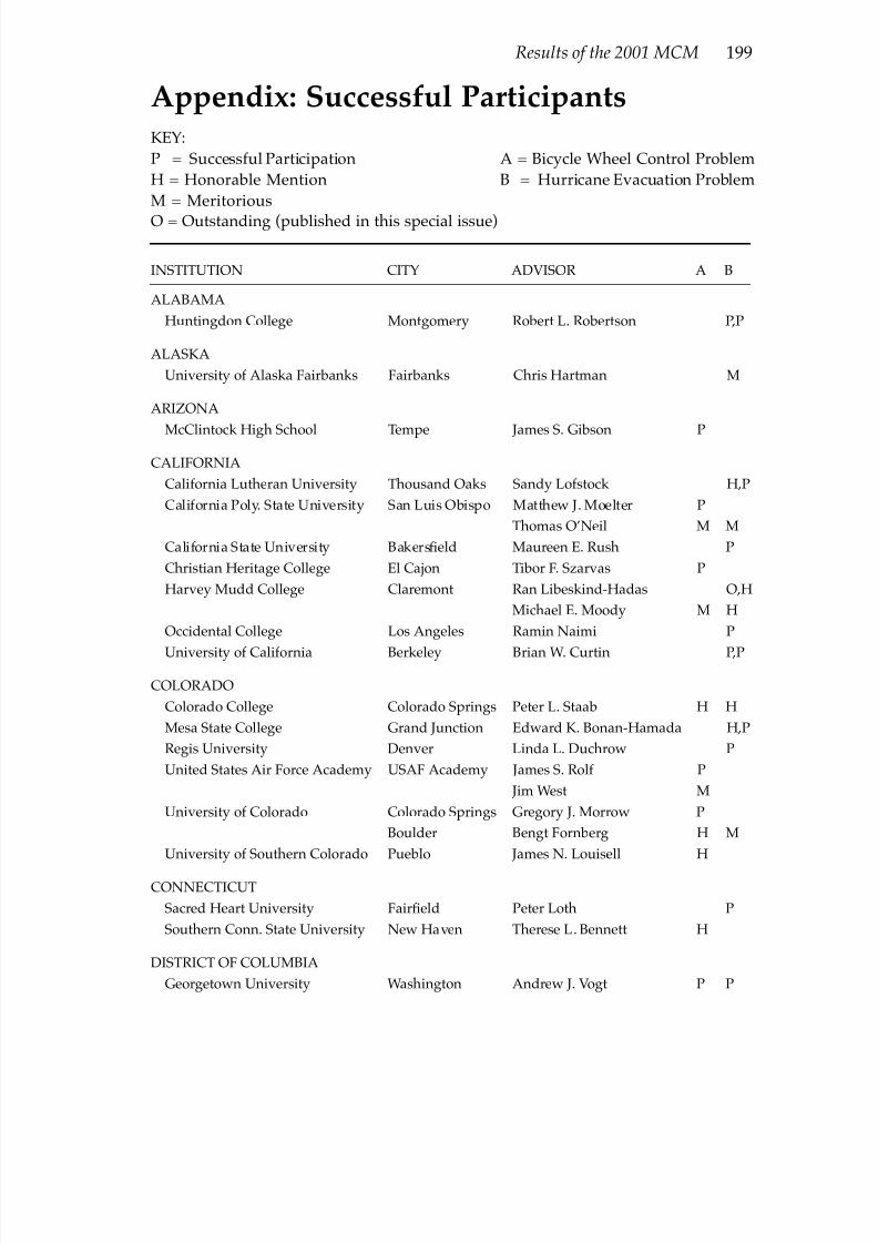
The nine papers that the judges designated as Outstanding appear in thisspecial issue of The UMAP Journal , together with commentaries. We list thoseteams and the Meritorious teams (and advisors) below; the list of all partici-pating schools, advisors, and results is in the Appendix.

7/17/2019 UMAP 2001 vol. 22 No. 3



Honorable Successful

Outstanding Meritorious Mention Participation Total

Bicycle Wheel 3 27 58 127 215

Hurricane Evacuation 6 43 65 167 281

9 70 123 294 496

Outstanding TeamsInstitution and Advisor Team Members

Bicycle Wheel Papers

“Spokes or Discs?”Stellenbosch UniversityMatieland, South Africa Jan H. van Vuuren

W.D.V. De WetD.F. MaianC. Mumbeck

“Selection of a Bicycle Wheel Type”United States Military AcademyWest Point, NYDonovan D. Phillips

Nicholas J. HowardZachariah R. MillerMatthew R. Adams

“A Systematic Technique for OptimalBicycle Wheel Selection”

University College Cork

Cork, Ireland James Jo Grannell

Michael Flynn

Eamonn LongWilliam Whelan-Curtin

Hurricane Evacuation Papers

“Project H.E.R.O.:Hurricane Evacuation Route Optimization”

Bethel CollegeSt. Paul, MNWilliam M. Kinney

“Traf Þc Flow Models andthe Evacuation Problem”

Duke UniversityDurham, NCDavid P. Kraines

Nathan M. GossettBarbara A. HessMichael S. Page

Samuel W. MaloneCarl A. MillerDaniel B. Neill

7/17/2019 UMAP 2001 vol. 22 No. 3



“The Crowd Before the Storm”The Governor’s SchoolRichmond, VA John A. Barnes

“Jammin’ with Floyd: A Traf Þc Flow Analysisof South Carolina Hurricane Evacuation”Harvey Mudd CollegeClaremont, CARan Libeskind-Hadas

“Blowin’ in the Wind”Lawrence Technological UniversitySouthÞeld, MIRuth G. Favro

“Please Move Quickly and Quietly to theNearest Freeway”

Wake Forest UniversityWinston-Salem, NCMiaohua Jiang

Jonathan D. CharlesworthFinale P. Doshi Joseph E. Gonzalez

Christopher HanusaAri NieMatthew Schnaider

Mark WagnerKenneth KoppWilliam E. Kolasa

Corey R. HoumandAndrew D. PruettAdam S. Dickey

Meritorious Teams

Bicycle Wheel Papers (27 teams)

Beijing University of Chemical Technology, Beijing, P.R. China (Jiang Guangfeng)

Beijing University of Chemical Technology, Beijing, P.R. China (Wenyan Yuan)

Brandon University, Brandon, Canada (Doug A. Pickering)

California Polytechnic State University, San Luis Obispo, CA (Thomas O’Neil)

Harbin Engineering University, Harbin, P.R. China (Gao Zhenbin)

Harbin Institute of Technology, Harbin, P.R. China (Shang Shouting)

Harvey Mudd College, Claremont, CA (Michael E. Moody)

James Madison University, Harrisonburg, VA (James S. Sochacki)

Jilin University of Technology, Changchun, P.R. China (Fang Peichen)

John Carroll University, University Heights, OH (Angela, S. Spalsbury)

Lafayette College, Easton, PA (Thomas Hill)

Lake Superior State University, Sault Sainte Marie, MI (J. Jaroma and D. Baumann)

Lewis and Clark College, Portland, OR (Robert W. Owens)Southeast University, Nanjing, P.R. China (Chen En-shui)

Tianjin University, Tianjin, P.R. China (Dong Wenjun)

Trinity University, San Antonio, TX (Fred M. Loxsom)

United States Air Force Academy, USAF Academy, CO (Jim West)

University College Dublin, Dublin, Ireland (Peter Duffy)

University of Western Ontario, London, Canada (Peter H. Poole)

Washington University, St. Louis, MO (Hiro Mukai)

7/17/2019 UMAP 2001 vol. 22 No. 3



Westminster College, New Wilmington, PA (Barbara T. Faires) (two teams)

Wright State University, Dayton, OH (Thomas P. Svobodny)

Youngstown State University, Youngstown, OH (Thomas Smotzer)

Zhejiang University, Hangzhou, P.R. China (He Yong)

Zhejiang University, Hangzhou, P.R. China (Yang Qifan)

Zhongshan University, Guangzhou, P.R. China (Chen Zepeng)

Hurricane Evacuation Papers (43 teams)

Beijing University of Posts & Telecommunications, Beijing, P.R. China (He Zuguo)

California Polytechnic State University, San Luis Obispo, CA (Thomas O’Neil)

Central South University, Changsha, P.R. China (Zheng Zhou-shun)

Clarion University, Clarion, PA (Jon A. Beal)

Dong Hua University, Shanghai, China (Ding Yongsheng)

East China University of Science & Technology, ShangHai, P.R. China (Liu Zhaohui)

Gettysburg College, Gettysburg, PA (Sharon L. Stephenson)

Hillsdale College, Hillsdale, MI (Robert J. Hesse) James Madison University, Harrisonburg, VA (Caroline Smith)

Jiading No. 1 High School, Jiading, P.R. China (Wang Yu)

MIT, Cambridge, MA (Dan Rothman)

N.C. School of Science and Mathematics, Durham, NC (Dot Doyle)

National University of Defence Technology, Changsha, P.R. China (Wu Mengda)

National University of Singapore, Singapore, Singapore

(Lim Leong Chye Andrew)

North Carolina State University, Raleigh, NC (Jeffrey S. Scroggs)

Northeastern University, Shenyang, P.R. China (Xiao Wendong)

PaciÞc Lutheran University, Tacoma, WA (Zhu Mei)

Päivölä College, Tarttila, Finland (Merikki Lappi)Rose-Hulman Institute of Technology, Terre Haute, IN (David J. Rader)

Rowan University, Glassboro, NJ (Paul J. Laumakis)

Shanghai Foreign Language School, Shanghai, P.R. China (Pan Li Qun)

South China University of Technology, Guangzhou, P.R. China (Lin Jianliang)

Southern Oregon University, Ashland, OR (Lisa M. Ciasullo)

U.S. Military Academy, West Point, NY (David Sanders)

U.S. Military Academy, West Point, NY (Edward Connors)

University of Alaska Fairbanks, Fairbanks, AK (Chris Hartman)

University of Colorado–Boulder, Boulder, CO (Bengt Fornberg)

University of Massachusetts Lowell, Lowell, MA (James Graham-Eagle)

University of North Texas, Denton, TX (John A. Quintanilla)

University of Richmond, Richmond, VA (Kathy W. Hoke)

University of Science and Technology of China, Hefei, P.R. China (Gu Jiajun)

University of South Carolina Aiken, Aiken, SC (Laurene V. Fausett)

University of South Carolina, Columbia, SC (Ralph E. Howard)

UniversityofSouthern Queensland,Toowoomba, Queensland,Australia(TonyJ. Roberts)

University of Washington, Seattle, WA (James Allen Morrow)

Wake Forest University, Winston-Salem, NC (Miaohua Jiang)

7/17/2019 UMAP 2001 vol. 22 No. 3



Washington University, St. Louis, MO (Hiro Mukai)

Western Washington University, Bellingham, WA (Saim Ural)

Worcester Polytechnic Institute, Worcester, MA (Bogdan Vernescu)

Wuhan University, Wuhan, P.R. China (Huang Chongchao)

York University, Toronto, Ontario, Canada (Juris Steprans)

Zhejiang University, Hangzhou, P.R. China (He Yong)Zhejiang University, Hangzhou, P.R. China (Yang Qifan)

Awards and Contributions

Each participating MCM advisor and team member received a certiÞcatesigned by the Contest Director and the appropriate Head Judge.

INFORMS, the Institute for Operations Research and the Management Sci-ences, gave a cash prize and a three-year membership to each member of the

teams from Stellenbosch University (Bicycle Wheel Problem) and LawrenceTechnological University (Hurricane Evacuation Problem). Also, INFORMSgave free one-year memberships to all members of Meritorious and HonorableMention teams. The Lawrence Tech team presented its results at the annualINFORMS meeting in Washington DC in April.

TheSociety for Industrial andApplied Mathematics (SIAM)designated oneOutstanding team from each problem as a SIAM Winner. The teams were fromU.S. Military Academy (Bicycle Wheel Problem) and Wake Forest University(Hurricane Evacuation Problem). Each of the team members was awarded a$300 cash prize and the teams received partial expenses to present their results

at a special Minisymposium of the SIAM Annual Meeting in San Diego CA in July. Their schools were given a framed, hand-lettered certiÞcate in gold leaf.TheMathematical Association of America (MAA) designated oneOutstand-

ing team from each problem as an MAA Winner. The teams were from Univer-sity College Cork (Bicycle Wheel Problem) and Wake Forest University (Hur-ricane Evacuation Problem). With partial travel support from the MAA, bothteams presented their solutions at a special session of the MAA Mathfest inMadison WI in August. Each team member was presented a certiÞcate byMAA President Ann Watkins.

JudgingDirectorFrank R. Giordano, COMAP, Lexington, MA

Associate DirectorsRobert L. Borrelli, Mathematics Dept., Harvey Mudd College,

Claremont, CA

7/17/2019 UMAP 2001 vol. 22 No. 3



Patrick Driscoll, Dept. of Mathematical Sciences, U.S. Military Academy,West Point, NY

William Fox, Mathematics Dept., Francis Marion University, Florence, SCMichael Moody, Mathematics Dept., Harvey Mudd College,

Claremont, CA

Bicycle Wheel Problem

Head JudgeMarvin S. Keener, Executive Vice-President, Oklahoma State University,

Stillwater, OK

Associate JudgesRonald Barnes, University of Houston Downtown, Houston TX (MAA)Kelly Black, Mathematics Dept., University of New Hampshire,

Durham, NH (SIAM)David Elliott, Institute for System Research, University of Maryland,

College Park, MD (SIAM)Ben Fusaro, Mathematics Dept., Florida State University,

Tallahassee, FLMario Juncosa, RAND Corporation, Santa Monica, CA John Kobza, Texas Tech University, Lubbock, TX (INFORMS)Dan Solow, Mathematics Dept., Case Western Reserve University,

Cleveland, OH (INFORMS)

Hurricane Evacuation Problem

Head JudgeMaynard Thompson, Mathematics Dept., University of Indiana,

Bloomington, IN

Associate JudgesPaul Boisen, National Security Agency, Ft. Meade, MD (Triage) James Case, Baltimore, MarylandCourtney Coleman, Mathematics Dept., Harvey Mudd College,

Claremont, CALisette De Pillis, Harvey Mudd College, Claremont, CAWilliam Fox, Dept. of Mathematical Sciences, U.S. Military Academy,

West Point, NY Jerry Griggs, University of South Carolina, Columbia, SC Jeff Hartzler, Mathematics Dept., Pennsylvania State University Middletown,

Middletown, PA (MAA)Deborah Levinson, Compaq Computer Corp., Colorado Springs, COVeena Mendiratta, Lucent Technologies, Naperville, ILDon Miller, Dept. of Mathematics, St. Mary’s College, Notre Dame, IN (SIAM)Mark R. Parker, Mathematics Dept., Carroll College, Helena, MT (SIAM)

7/17/2019 UMAP 2001 vol. 22 No. 3



John L. Scharf, Carroll College, Helena, MTLee Seitelman, Glastonbury, CT (SIAM)Kathleen M. Shannon, Salisbury State University, Salisbury, MDMichael Tortorella, Lucent Technologies, Holmdel, NJMarie Vanisko, Carroll College, Helena, MT

Cynthia J. Wyels, Dept. of Mathematics, Physics, and Computer Science,California Lutheran University, Thousand Oaks, CA

Triage Sessions:

Bicycle Wheel Problem

Head Triage JudgeTheresa M. Sandifer, Southern Connecticut State University, New Haven, CT

Associate JudgesTherese L. Bennett, Southern Connecticut State University, New Haven, CT

Ross B. Gingrich, Southern Connecticut State University, New Haven, CTCynthia B. Gubitose, Western Connecticut State University, Danbury, CTRon Kutz, Western Connecticut State University, Danbury, CTC. Edward Sandifer, Western Connecticut State University, Danbury, CT

Hurricane Evacuation Problem

Head Triage JudgePaul Boisen, National Security Agency, Ft. Meade, MD

Associate Judges

James Case, Baltimore, MarylandPeter Anspach, Jennifer Mcgreevy, Erin Schram, Larry Wargo, and 7 othersfrom the National Security Agency

Sources of the Problems

The Bicycle Wheel Problem was contributed by Kelly Black, MathematicsDept., University of New Hampshire, Durham, NH.TheHurricaneEvacuationProblem was contributed by Jerry Griggs, Mathematics Dept., University of South Carolina, Columbia, SC.

Acknowledgments

The MCM was funded this year by the National Security Agency, whosesupport we deeply appreciate. We thank Dr. Gene Berg of NSA for his coordi-nating efforts. The MCM is also indebted to INFORMS, SIAM, and the MAA,which provided judges and prizes.

7/17/2019 UMAP 2001 vol. 22 No. 3



I thank the MCM judges and MCM Board members for their valuable andunßagging efforts. Harvey Mudd College, its Mathematics Dept. staff, andProf. Borrelli were gracious hosts to the judges.

CautionsTo the reader of research journals:

Usually a published paper has been presented to an audience, shown tocolleagues, rewritten, checked by referees, revised, and edited by a journaleditor. Each of the student papers here is the result of undergraduates workingon a problem over a weekend; allowing substantial revision by the authorscouldgive a false impressionofaccomplishment. Sothesepapersare essentiallyau naturel. Light editing has taken place: minor errors have been corrected,wording has been altered for clarity or economy, and style has been adjusted to

that of The UMAP Journal. Please peruse these student efforts in that context.

To the potential MCM Advisor:

It might be overpowering to encounter such output from a weekend of work by a small team of undergraduates, but these solution papers are highlyatypical. A team that prepares and participates will have an enriching learningexperience, independent of what any other team does.

7/17/2019 UMAP 2001 vol. 22 No. 3



Appendix: Successful ParticipantsKEY:

P = Successful ParticipationH = Honorable Mention

M = Meritorious

A = Bicycle Wheel Control ProblemB = Hurricane Evacuation Problem

O = Outstanding (published in this special issue)

INSTITUTION CITY ADVISOR A B

ALABAMA

Huntingdon College Montgomery Robert L. Robertson P,P

ALASKA

University of Alaska Fairbanks Fairbanks Chris Hartman M

ARIZONA

McClintock High School Tempe James S. Gibson P

CALIFORNIA

California Lutheran University Thousand Oaks Sandy Lofstock H,P

California Poly. State University San Luis Obispo Matthew J. Moelter P

Thomas O’Neil M M

California State University BakersÞeld Maureen E. Rush P

Christian Heritage College El Cajon Tibor F. Szarvas P

Harvey Mudd College Claremont Ran Libeskind-Hadas O,H

Michael E. Moody M H

Occidental College Los Angeles Ramin Naimi P

University of California Berkeley Brian W. Curtin P,P

COLORADO

Colorado College Colorado Springs Peter L. Staab H H

Mesa State College Grand Junction Edward K. Bonan-Hamada H,P

Regis University Denver Linda L. Duchrow P

United States Air Force Academy USAF Academy James S. Rolf P

Jim West M

University of Colorado Colorado Springs Gregory J. Morrow P

Boulder Bengt Fornberg H M

University of Southern Colorado Pueblo James N. Louisell H

CONNECTICUT

Sacred Heart University FairÞeld Peter Loth P

Southern Conn. State University New Haven Therese L. Bennett H

DISTRICT OF COLUMBIA

Georgetown University Washington Andrew J. Vogt P P

7/17/2019 UMAP 2001 vol. 22 No. 3




FLORIDA

Embry-Riddle Aero. University Daytona Beach Greg Scott Spradlin P,P

Florida A&M University Tallahassee Bruno Guerrieri P P

Stetson University DeLand Lisa O. Coulter PUniversity of North Florida Jacksonville Peter A. Braza P

GEORGIA

Agnes Scott College Decatur Robert A. Leslie P,P

Georgia Southern University Statesboro Goran Lesaja H,P

State University of West Georgia Carrollton Scott Gordon P

IDAHO

Albertson College of Idaho Caldwell Mike Hitchman P

Boise State University Boise Jodi L. Mead P

ILLINOIS

Greenville Colllege Greenville Galen R. Peters H,P

Illinois Wesleyan University Bloomington Zahia Drici P,P

Northern Illinois University DeKalb Emil Cornea P

Wheaton College Wheaton Paul Isihara H,P

INDIANA

Goshen College Goshen David Housman H,H

Indiana University Bloomington Michael S. Jolly H

Rose-Hulman Inst. of Technology Terre Haute David J. Rader M,P

Frank Young HSaint Mary’s College Notre Dame Peter D. Smith H,P

IOWA

Grand View College Des Moines Sergio Loch P P

Grinnell College Grinnell Marc A. Chamberland H H

Mark Montgomery P,P

Luther College Decorah Reginald D. Laursen H,P

Mt. Mercy College Cedar Rapids K.R. Knopp H

Simpson College Indianola Murphy Waggoner P P

Werner S. Kolln H

Wartburg College Waverly Mariah Birgen P,P

KANSAS

Emporia State University Emporia Ton Boerkoel P

Kansas State University Manhattan Korten N. Auckly P

KENTUCKY

Asbury College Wilmore Kenneth P. Rietz H H

Spalding University Louisville Scott W. Bagley P

7/17/2019 UMAP 2001 vol. 22 No. 3




LOUISIANA

Northwestern State University Natchitoches Richard C. DeVault P

MAINE

Colby College Waterville Jan Holly H

MARYLAND

Goucher College Baltimore Robert E. Lewand H,P

Johns Hopkins University Baltimore Daniel Q. Naiman P

Mount Saint Mary’s College Emmitsburg William E. O’Toole P

Fred Portier P

Salisbury State University Salisbury Steven M. Hetzler H

Michael J. Bardzell P

MASSACHUSETTS

MIT Cambridge Dan Rothman M,H

Salem State College Salem Kenny Ching P

Smith College Northampton Ruth Haas P

University of Massachusetts Lowell James Graham-Eagle P M

Williams College Williamstown Stewart D. Johnson P

Frank Morgan P

Cesar E. Silva P

Worcester Poly. Inst. Worcester Bogdan Vernescu M

MICHIGAN

Calvin College Grand Rapids Randall J. Pruim P

Eastern Michigan University Ypsilanti Christopher E. Hee P P

Hillsdale College Hillsdale Robert J. Hesse M

Lake Superior State University Sault Sainte Marie John Jaroma and

David Baumann M

Lawrence Tech. University SouthÞeld Ruth G. Favro O

Scott Schneider H

Howard Whitston P

Siena Heights University Adrian Toni Carroll P,P

Rick V. Trujillo P

University of Michigan Dearborn David James P

MINNESOTA

Bemidji State University Bemidji Colleen G. Livingston P,P

Bethel College St. Paul William M. Kinney O

Macalester College St. Paul A. Wayne Roberts P P

St. Olaf College NorthÞeld Philip J. Gloor P

University of Minnesota Morris Peh H. Ng P

7/17/2019 UMAP 2001 vol. 22 No. 3




MISSOURI

Crowder College Neosho Cheryl L. Ingram P

Missouri Southern State College Joplin Patrick Cassens P P

Northwest Missouri State Univ. Maryville Russell N. Euler P PSoutheast Missouri State Univ. Cape Girardeau Robert W. Sheets H

Truman State University Kirksville Steve Jay Smith P

Washington University St. Louis Hiro Mukai M M

Wentworth Mil. Acad. & Jr. Coll. Lexington Jacqueline O. Maxwell P P

MONTANTA

Carroll College Helena Philip B. Rose P

Holly S. Zullo P P

St. Andrew University Helena Mark J. Keeffe P

NEBRASKA

Hastings College Hastings David B. Cooke P

University of Nebraska Lincoln Glenn W. Ledder H

NEVADA

University of Nevada Reno Mark M. Meerschaert P

NEW JERSEY

Montclair State University Upper Montclair Michael A. Jones P

Rowan University Glassboro Paul J. Laumakis M

NEW YORK

Hunter College, City Univ. of NY New York Ada Peluso HIthaca College Ithaca John C. Maceli P

Manhattan College Riverdale Kathryn C. Weld P

Marist College Poughkeepsie Tracey B. McGrail P

State University of NY Cortland George F. Feissner P

R. Bruce Mattingly P

U.S. Military Academy West Point Edward Connors M

Gregory Parnell H

Donovan D. Phillips O

David Sanders M

Westchester Comm. College Valhalla Sheela L. Whelan P,P

NORTH CAROLINA

Appalachian State University Boone Holly P. Hirst H

Eric S. Marland P

Brevard College Brevard Clarke Wellborn P,P

Davidson College Davidson Laurie J. Heyer H

Duke University Durham David P. Kraines O

N.C. School of Sci. & Math. Durham Dot Doyle M

7/17/2019 UMAP 2001 vol. 22 No. 3




North Carolina State Univ. Raleigh Jeffrey S. Scroggs M,H

University of North Carolina Wilmington Russell L. Herman P

Wake Forest University Winston-Salem Miaohua Jiang O,M

Western Carolina University Cullowhee Jeffrey Allen Graham P

OHIO

The College of Wooster Wooster Pamela Pierce P

Hiram College Hiram Brad S. Gubser H

John Carroll University University Heights Angela S. Spalsbury M P

Miami University Oxford Doug E. Ward P

Oberlin College Oberlin Elizabeth L. Wilmer P

Ohio University Athens David N. Keck P

Wright State University Dayton Thomas P. Svobodny M,P

Youngstown State University Youngstown Stephen Hanzely P

Robert Kramer PThomas Smotzer M H

OKLAHOMA

Oklahoma State University Stillwater John E. Wolfe P,P

Southern Nazarene Univ. Bethany Virgil Lee Turner H

Univ. of Central Oklahoma Edmond Charles Cooper P

Dan Endres P

OREGON

Eastern Oregon University La Grande Robert Huotari HAnthony Tovar H,P

Jennifer Woodworth P

Lewis & Clark College Portland Robert W. Owens M

Portland State University Portland Gerardo A. Lafferriere H,P

Southern Oregon University Ashland Lisa M. Ciasullo M

University of Portland Portland Thomas W. Judson P

PENNSYLVANIA

Bloomsburg University Bloomsburg Kevin K. Ferland P H

Clarion University Clarion Jon A. Beal M

John W. Heard PGettysburg College Gettysburg James P. Fink H H

Carl Leinbach H

Sharon L. Stephenson M

Lafayette College Easton Thomas Hill M

Shippensburg University Shippensburg Cheryl Olsen P

Villanova University Villanova Bruce Pollack-Johnson P

Westminster College New Wilmington Barbara T. Faires M,M

7/17/2019 UMAP 2001 vol. 22 No. 3




RHODE ISLAND

Rhode Island College Providence David L. Abrahamson P

SOUTH CAROLINA

Charleston Southern University Charleston Stan Perrine P,P

Coastal Carolina University Conway Ioana Mihaila P

Francis Marion University Florence Thomas L. Fitzkee P

Midlands Technical College Columbia SJohn R. Long P

University of South Carolina Aiken Laurene V. Fausett M,P

Columbia Ralph E. Howard M

SOUTH DAKOTA

Mount Marty College Yankton Jim Miner P

S.D. School of Mines & Tech. Rapid City Kyle L. Riley P P

TENNESSEEChristian Brothers University Memphis Cathy W. Carter P

Lipscomb University Nashville Mark A. Miller P

TEXAS

Abilene Christian University Abilene David Hendricks H

Angelo State University San Angelo Trey Smith H

Baylor University Waco Frank H. Mathis H

Southwestern University Georgetown Therese N. Shelton P

Stephen F. Austin State University Nacogdoches Colin L. Starr P

Trinity University San Antonio Allen G. Holder P

Jeffrey K. Lawson P

Fred M. Loxsom M

Hector C. Mireles P

University of Houston Houston Barbara Lee KeyÞtz P

University of North Texas Denton John A. Quintanilla M

University of Texas Austin Lorenzo A. Sadun P

UTAH

Weber State University Ogden Richard R. Miller H

VERMONT

Johnson State College Johnson Glenn D. Sproul P P

VIRGINIA

Eastern Mennonite University Harrisonburg John Horst P H

The Governor’s School Richmond John A. Barnes P O

Crista Hamilton H,P

James Madison University Harrisonburg Caroline Smith M

James S. Sochacki M

Randolph-Macon College Ashland Bruce F. Torrence P

7/17/2019 UMAP 2001 vol. 22 No. 3




Roanoke College Salem Jeffrey L. Spielman H

University of Richmond Richmond Kathy W. Hoke M

Univ. of Virginia’s College at Wise Wise George W. Moss P P

Virginia Western Comm. College Roanoke Steve T. Hammer H

Ruth A. Sherman P

WASHINGTON

PaciÞc Lutheran University Tacoma Mei Zhu H M

University of Puget Sound Tacoma DeWayne R. Derryberry P P

Carol M. Smith P

University of Washington Seattle Randall J. LeVeque H

James Allen Morrow M

Wenatchee Valley College Omak Kit A. Arbuckle P

Western Washington University Bellingham Saim Ural MTjalling Ypma H,H

WEST VIRGINNIA

West Virginia Wesleyan College Buckhannon Jeffery D. Sykes P

WISCONSIN

Beloit College Beloit Paul J. Campbell P

Ripon Ripon College David W. Scott P

Univ. of Wisconsin–Stevens Point Stevens Point Nathan R. Wetzel P

Univ. of Wisconsin–Stout Menomonie Maria G. Fung H

Wisconsin Lutheran College Milwaukee Marvin C. Papenfuss P

AUSTRALIA

University of New South Wales Sydney, NSW James Franklin H,H

University of Southern Queensland Toowoomba, QLD Tony J. Roberts M

CANADA

Brandon University Brandon, MB Doug A. Pickering M

Dalhousie University Halifax, NS John C. Clements P

Dorette A. Pronk P

Memorial Univ. of Newfoundland St. John’s, NF Andy Foster P

University of Saskatchewan Saskatoon, SK James A. Brooke H,P

Tom G. Steele H

University of Toronto Toronto, ON Nicholas A. Derzko P

University of Western Ontario London, ON Peter H. Poole M,P

York University Toronto, ON Juris Steprans M,H

CHINA

Anhui Mechanical and Electronics Wuhu Wang Chuanyu P

College Wang Geng P

Yang Yimin P

7/17/2019 UMAP 2001 vol. 22 No. 3




Anhui University Hefei Cai Qian P

Wang Da-peng H

Zhang Quan-bing P

Beijing Institute of Technology Beijing Chen Yihong H PCui Xiaodi P,P

Yao Cuizhen H P

Beijing Union University Beijing Jiang Xinhua P

Ren Kailong P

Wang Xinfeng P

Zeng Qingli P

Beijing University of Aero. & Astronautics Beijing Peng Linping H,H

Wu Sanxing P,P

Beijing University of Chemical Technology Beijing Cheng Yan P

Jiang Guangfeng MLiu Daming P

Wenyan Yuan M

Beijing University of Posts & Telecomm. Beijing He Zuguo M,H

Luo Shoushan P,P

Central South University Changsha Zhang Hong-yan P

Zheng Zhou-shun M

China University of Mining & Technology Xuzhou Wu Zongxiang P P

Zhu Kaiyong P P

Chongqing University Chongqing Gong Qu P H

Li Fu P

Zhan Lezhou H

Dalian University of Technology Dalian Ding Yongsheng M

He Mingfeng H P

Yu Hongquan H

Dong Hua University Shanghai Hu Liangjian H

Lu Yunsheng P

East China Normal University Shanghai Jiang Lumin P

Zhen Dong Yuan P

East China Univ. of Science and Technology Shanghai Liu Zhaohui M

Lu Yuanhong H

Qin Yan HShi Jinsong H

Fudan University Shanghai Cai Zhijie P,P

Gong XueQing P P

Xu Qinfeng P

Guangdong Commercial College Guangzhou Xiang Zigui P P

7/17/2019 UMAP 2001 vol. 22 No. 3




Harbin Engineering University Harbin Gao Zhenbin M

Luo Yuesheng H

Shen Jihong P

Zhang Xiaowei PHarbin Institute of Technology Harbin Shang Shouting M P

Shao Jiqun H

Wang Xuefeng P

Hefei University of Technology Hefei Du Xueqiao P H

Huang Youdu P,P

Hu Ning (individual, one-member team) Suzhou P

Information & Engineering University Zhengzhou Han Zhonggeng P

Li Bin P

Lu Zhibo P

Zhang Wujun H

Jiading No. 1 High School Jiading Chen Gan P

Wang Yu M

Jiamusi University Jiamusi Bai Fengshan P

Fan Wui P

Gu Lizhi P

Liu Yuhui P

Jilin University of Technology Changchun Fang Peichen M P

Yang Yinsheng P,P

Jinan University Guangzhou Hu Daiqiang P

Ye Shi Qi P P

Nanjing Nankai University Tianjin Liang Ke H

Ruan Jishou P,P

Zhou Xingwei H

Nanjing Normal University Nanjing Chen Bo P

Chen Xin P

Fu Shitai P

Zhu Qun-Sheng P

Nanjing University Nanjing Yao Tianxing H,P

Nanjing University of Science & Technology Nanjing Wu Xingming P

Xu Chun Gen H

Yang Jian PYu Jun P

Nankai University Tianjin Ke Liang H

Ruan Jishou P,P

Zhou Xingwei H

National University of Defence Technology Changsha Lu Shirong H P

Wu Mengda H M

North China Institute of Technology Taiyuan Lei Ying-jie P

Xue Ya-kui P

Yong Bi H

7/17/2019 UMAP 2001 vol. 22 No. 3




Northeastern University Shenyang Cui Jianjiang P

Han Tie-min P

Hao Peifeng P

Xiao Wendong MXue Dingyu P

Northwest Inst. of Texile Sci. & Tech. Xi’an He XingShi P H

Northwest University Xi’an He Rui-chan P,P

Northwestern Polytechnic University Xi’an Hua Peng Guo H

Liu Xiao Dong H

Shi Yi Min H

Zhang Sheng Gui P

Peking University Beijing Deng Minghua P P

Lei Gongyan H,P

Shu Yousheng H H

Second Aero. Inst. of the Air Force ChangChun Zhang Shaohuai and

Fu Deyou P,P

Shandong University Jinan Ma Piming P

Ma Zhengyuan P

Shanghai Foreign Language School Shanghai Li Qun Pan M,P,P

Shanghai Jiaotong University Shanghai Huang Jianguo P,P

Song Baorui H P

Shanghai Maritime University Shanghai Sheng Zining P

Shanghai Normal University Shanghai Guo Shenghuan P

Zhang Jizhou P

Zhu Detong H

Shanghai Univ. of Finance and Econ. Shanghai Feng Suwei H

Yang Xiaobin H

Shanxi University Taiyuan Li Jihong P

Yang Aimin P

Zhang Xianwen P

Zhao Aimin P

Sichuan University Chengdu Li Huang P

Liu Xiaoshi P

Yang Zhihe P

Zhou Jie PSouth China University of Technology Guangzhou Liang Manfa P

Lin Jianliang M

Tao Zhisui H

Zhu Fengfeng H

Southeast University Nanjing Chen En-shui M P

Huang Jun H,H

Tianjin University Tianjin Dong Wenjun M

Liu Zeyi P

Wenhua Hou P

7/17/2019 UMAP 2001 vol. 22 No. 3




Tsinghua University Beijing Hu Zhi-Ming P H

Ye Jun H H

University of Elec. Science & Tech. Chengdu Wang Jiangao P H

Xu Quanzhi PZhong Erjie P

University of Sci. & Tech. of China Hefei Gu Iajun M

Yang Jian H

Yang Liu P

Yong Ni P

Wuhan University (WUHEE) Wuhan Chen Gui Xing P

Huang Chongchao M

Wuhan University of Tech. Wuhan Huang Zhang-Can P

Xi’an Inst. of Post & Telecomm. Xi’an Li Changxing and

Fan Jiulun P

Xi’an Jiaotong University Xi’an Dai Yonghong P

Zhou Yicang H

Xi’an University of Technology Xi’an Cao Maosheng P P

Xidian University Xian Chen Hui-chan H

Liu Hong-wei H

Zhang Zhuo-kui H

Zhou Shui-sheng P

YanShan University QinHuangDao Wang YongMao P

Zhong XiaoZhu P P

Zhejiang University Hangzhou He Yong M M

Yang Qifan M M

Zhongshan University Guangzhou Bao Yun H

Chen Zepeng M

Li Caiwei H

Yin Xiaoling P

ENGLAND

University of Oxford Oxford Maciek Dunajski H

FINLAND

Päivölä College Tarttila Merikki Lappi M,H

HONG KONG

Hong Kong Baptist University Kowloon Tong W.C. Shiu H

C.S. Tong P

IRELAND

National University of Ireland Galway Niall Madden P H

Trinity College Dublin Dublin Timothy G. Murphy H

University College Cork Cork James Joseph Grannell O

Donal J. Hurley H

Brian J. Twomey H

7/17/2019 UMAP 2001 vol. 22 No. 3




University College Dublin Dublin Peter Duffy M

Maria G. Meehan P,P

LITHUANIA

Vilnius University Vilnius Ricardas Kudzma P

SINGAPORE

National Univ. of Singapore Singapore Lim Leong Chye Andrew M

SOUTH AFRICA

Stellenbosch University Matieland Jan H. van Vuuren O H

Editor’s NoteFor team advisors fromChina and Singapore, we have endeavored tolist familyname Þrst, with the help of Susanna Chang ’03.

7/17/2019 UMAP 2001 vol. 22 No. 3


Spokes or Discs? 211

Spokes or Discs?

W.D.V. De WetD.F. Malan

C. Mumbeck Stellenbosch UniversityMatieland, Western CapeSouth Africa

Advisor: Jan H. van Vuuren

Introduction

It is well known that disc wheels and standardspoked wheels exhibit differ-ent performance characteristics on the race track, but as yet no reliable meansexist to determine which is superior for a given set of conditions.

We create a model that, taking the properties of wheel, cyclist, and courseinto account, may provide a deÞnitive answer to the question, “Which wheelshould I use today?” The model provides detailed output on wheel perfor-mance and can produce a chart indicating which wheel will provide optimalperformance for a given environmental and physical conditions.

We use laws of physics, plus data from various Web sites and publishedsources, then numerical methods to obtain solutions from the model.

We demonstrate the use of the model’s output on a sample course. Roughly

speaking, standard spoked wheels perform better on steep climbs and trailing winds,while disc wheels are better in most other cases.

We did some validation of the model for stability, sensitivity, and realism.We also generalised it to allow for a third type of wheel, to provide a morerealistic representation of the choice facing the professional cyclist today.

A major dif Þculty was obtaining reliable data; sources differed or even con-tradicted one another. The range of the data that we couldÞndwas insuf Þcient, jeopardizing the accuracy of our results.

TheUMAPJournal22 (3)(2000)211–223. cCopyright 2001 by COMAP, Inc. All rights reserved.Permission to make digital or hard copies of part or all of this work for personal or classroom useis granted without fee provided that copies are not made or distributed for proÞt or commercialadvantage and that copies bear this notice. Abstracting with credit is permitted, but copyrightsfor components of this work owned by others than COMAP must be honored. To copy otherwise,to republish, to post on servers, or to redistribute to lists requires prior permission from COMAP.

7/17/2019 UMAP 2001 vol. 22 No. 3



Analysis of the Problem

Consider the system of a cyclist and the racing cycle. The cyclist providesthe energy to drive the bicycle against the forces of drag (from contact with air),friction (fromcontact between wheelsand ground),andgravity (whichopposes

progress up a slope). Furthermore, when accelerating, the cyclist must providethe energy to set the wheels rotating, due to their moment of inertia.

The primary problem is to determine, for a given set of conditions, whichtype of rear wheel is the most effective. “Effectiveness” is what a speciÞc riderdesires from the equipment. We assume that the rider desires to completethe course in as short a time as possible, or with the least possible energyexpenditure. These deÞnitions are closely linked: A rider who expends moreenergy to maintain a certain speed will soon tireand will therefore have a lowermaintainable speed.

The differences between standard 32-spoke wheels and disc wheels lie inweight and in their aerodynamic properties. Given the right wind conditions

(whichweinvestigate), thediscwheelsshould allowairtopass thecyclist/cyclecombination with less turbulence, that is, less drag. However, disc wheelsweigh more, which affects the amountof power requiredtomove the wheels upa slope and to begin rotating the wheels from rest (such as when accelerating).

To examine which type of wheel performs the best under which conditions,we need to determine which wheel allows the greatest speed given speciÞcconditions or, equivalently, which wheel requires the least power to drive.

Thegreatest dif Þculty is that air resistance is a function of speed while speedis a function of air resistance. The model needs to utilise numerical methods tocalculate the speed that a rider can maintain with the given parameters.

There are other factors to consider, too. Disc wheels are not very stable ingusty wind conditions, since they provide a far greater surface area to cross-winds; with a greater moment of inertia, they accelerate more slowly; and theirgreater weight may provide more grip on wet roads.

Assumptions and Hypothesis

We investigated the performance of the wheel types noted in Table 1. Thewheel data do not conform to any speciÞc make or model but are typical.

Table 1.Types of wheels.

Type Standard 32-spoke Aero wheel (trispoke) Solid disc wheel

Diameter (m) 0.7 0.7 0.7Mass (kg) 0.8 1.0 1.3

We assume that the cyclist uses a standard spoke wheel in the front andeither a disc wheel or standard 32-spoked wheel at the back. We also brießy

7/17/2019 UMAP 2001 vol. 22 No. 3



examine aero wheels, which are not solid but more aerodynamic than standardspoked wheels. We refer to the three types as standard, aero, and disc.

We assume that the rider and cycle frame (excluding wheels) exhibit thesame drag for all wind directions.

Table 2.Symbols used.

Symbol Unit DeÞnition

A m2 area of rider/bicycle exposed to wind

ca dimensionless variable coef Þcient of axial air resistance for speciÞc wheelcrr dimensionless constant of rolling resistancecw dimensionless constant of air resistanceD m2 reference area of wheelF ad Newton (N) axial air resistance

(against the cyclist’s direction of motion)F ∗ad

Newton (N) axial air resistance on a bicycle with box-rimmed spoked wheels in aheadwind

F g Newton (N) effect of gravity on the cyclistF rr Newton (N) rolling resistanceg m/s2 gravitational constantM kg mass of cyclist and cycleP Watt (W) rider’s effective power outputvbg m/s speed of the bike relative to the groundvwb m/s speed of the wind relative to the bikevwg m/s speed of the wind relative to the groundα degree angle of the riseβ degree yaw angle, the angle between the direction

opposing bicycle motion and perceived wind(A relative headwind has a yaw of 0◦.)

γ degree angle between wind direction (vwg ) and direction of motion

(A straight-on headwind has γ = 180◦

.)ψ percent grade of hill, the sine of α , the angle of the riseρ kg/m3 air density

Forces at Work

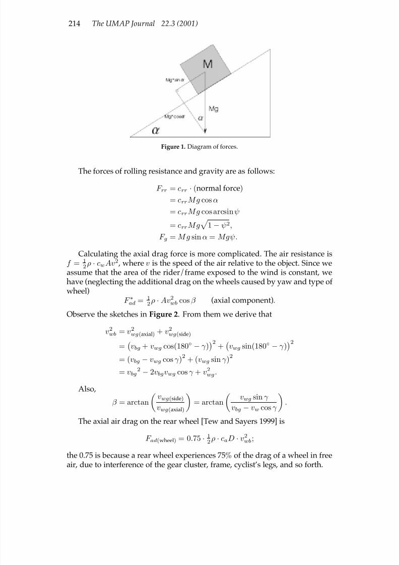
For a bicycle moving at a constant velocity, there are three signiÞcant re-tarding forces (Figure 1):

rolling resistance, due to contact between the tires and road;

gravitational resistance, if the road is sloped; and

air resistance, usually the largest of the three.

When accelerating, the rider also uses energy to overcome translational androtational inertia, although the model does not take these into account.

7/17/2019 UMAP 2001 vol. 22 No. 3



Figure 1. Diagram of forces.

The forces of rolling resistance and gravity are as follows:

F rr = crr

·(normal force)

= crrMg cos α

= crrMg cos arcsin ψ

= crrMg

1− ψ2,

F g = M g sin α = Mgψ.

Calculating the axial drag force is more complicated. The air resistance isf = 1

2ρ · cwAv2 , where v is the speed of the air relative to the object. Since weassume that the area of the rider/frame exposed to the wind is constant, wehave (neglecting the additional drag on the wheels caused by yaw and type of wheel)

F ∗ad = 12ρ · Av2wb cos β (axial component).

Observe the sketches in Figure 2. From them we derive that

v2wb = v2wg(axial) + v2wg(side)

=

vbg + vwg cos(180◦ − γ )2

+

vwg sin(180◦ − γ )2

= (vbg − vwg cos γ )2

+ (vwg sin γ )2

= vbg2 − 2vbgvwg cos γ + v2wg .

Also,

β = arctan

vwg(side)

vwg(axial)

= arctan

vwg sin γ

vbg − vw cos γ

.

The axial air drag on the rear wheel [Tew and Sayers 1999] is

F ad(wheel) = 0.75 · 12ρ · caD · v2wb;

the 0.75 is because a rear wheel experiences 75% of the drag of a wheel in freeair, due to interference of the gear cluster, frame, cyclist’s legs, and so forth.

7/17/2019 UMAP 2001 vol. 22 No. 3



Figure 2a. Wind speed relative to wheel.

Figure 2b. Forces on wheel.

For the three basic types of wheel, Tew and Sayers [1999] give typical curvesof the axial drag coef Þcient ca vs. yaw angle (0◦ ≤ β ≤ 30◦); this intervalaccounts for the majority of conditions experienced by a rider. We approximatethese curves by straight lines (a close match).

The curves for different relative wind speeds are very much alike for thestandard wheel and the aero wheel. The disc wheel, however, shows majorvariation for different relative wind speeds.

Since the axial drag coef Þcient must be zero at β = 90◦ , and by observingthe shape of the curves, we extrapolated to larger yaw angles using a sine-shaped curve through ca = 0 at β = 90◦ , with an appropriate scaling to ensurecontinuity. Without wind-tunnel testing, the accuracy cannot be guaranteed.

Comparing the percentage of power dissipated by drag on one wheel (ac-cording to the model) with the data of Tew and Sayers [1999], we found a highdegree of agreement. Typically, 1% to 10% (depending on wheel type) of thepower is dissipated by drag on the wheels.

From F ad(wheel) we subtracted the drag experienced by a normal (box-rimmed) wheel under headwind, since it was already taken account in F ∗ad.

7/17/2019 UMAP 2001 vol. 22 No. 3



The axial air drag on the bicycle is thus given by

F ad = F ∗ad + F ad(wheel) = 12ρv2wb[cwA cos β + 0.75(ca − 0.06)D],

where 0.06 is the coef Þcient of axial drag for a normal wheel in a headwind.The cos β gives the component in the direction of motion of the cyclist.

Calculating Results for a Typical Rider

For data, we used standard values [Analytic Cycling 2001] for a road racernear sea level in normal atmospheric conditions:

M = 80 kg, g = 9.81 m/s2,

crr = 0.004, cw = 0.5,

A = 0.5 m2, D = 0.38 m2 (for a 700 mm wheel),

ρ = 1.226 kg/m3 (could be changed to incorporate altitude).

We calculated that, to maintain a speed of 45 km/h on a level road (as inthe problem description), the rider must deliver 340 W of effective pedalingpower.

The Computer Program

We wrote a computer program in Pascal that calculates the speed that the

rider can sustain for a given vwg , γ , and ψ. It does this by trying a speed anddetermining the wattage necessary to sustain the speed. If the wattage is toohigh, the speed is lowered; otherwise, the speed is increased. Every time thesolution point is crossed, the step size is reduced. The process is carried outuntil the wattage used is within a tolerance 0.01 W to P .

To take into account the effect of drag on different types of wheels, ourprogram does the following:

1. The wind direction, wind speed relative to the ground, and slope of the road(γ , vwg , and ψ) are provided as inputs.

2. The program tries a value for vbg.

3. F rr and F g are calculated.

4. From γ , vwg , ψ , and vbg , we calculate vwb and β .

5. From vwb and β , we calculate F ad.

6. We calculate the wattage by using the formula P = (F rr + F g + F ad)vbg.

7. We compare the calculated value of P to the known value of 340 W.

7/17/2019 UMAP 2001 vol. 22 No. 3



8. We try a new value for vbg , depending on whether the wattage required forthe previous value of vbg was higher or lower than the available 340 W.

9. We repeat this process from Step 3 until the maximum maintainable speedis determined.

Since the wheel that requires the least power in a set of circumstances alsoenables the highest speed, we used our program to vary the speed of the windand show which wheel is best for the circumstances. Figure 3 shows a screenshot. The dark colour represents blue and the light colour red. Each of the 11horizontal strips represents a road gradient, ranging from 0 at the top to 0.1 atthe bottom in 0.01 increments.

Figure 3. Screen shot from program.

The horizontal axis is wind speed, from 0 km/h at the left to 63.9 km/h atthe right in 0.1 km/h increments. The vertical axis of each bar is the wind angle(relative to track), from 0◦ to 180◦ in 15◦ increments.

We have a very compact representation showing the transition wind speedsfor a range of wind angles and road gradients. The user is provided a crosshairto move over any point on the graph. The colour of a pixel indicates the betterwheel to use for the corresponding gradient, wind speed, and wind angle.

To generate a table of transition speeds (Table 3), we read off the pointsat which transitions occur. This might seem cumbersome, but developing analgorithm toÞnd the transition points is very dif Þcult, since the numberof tran-sitions is not known beforehand and the functions exhibit irregular behaviour.

To use the table, look up the particular entry corresponding to the roadgrade and the angle that the wind makes with the forward direction of the bike. An entry of S means that a standard wheel performs better for all windspeeds, a D indicates that a disc wheel is better at all wind speeds.

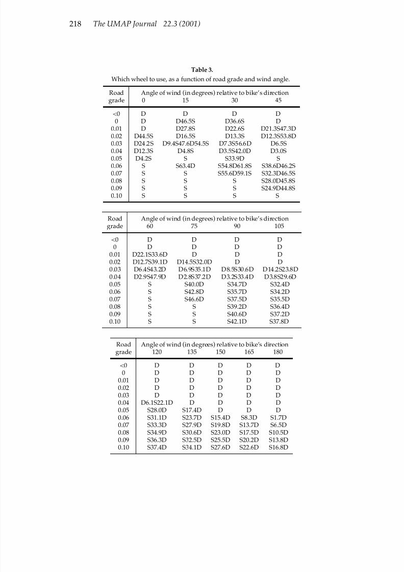
7/17/2019 UMAP 2001 vol. 22 No. 3



Table 3.

Which wheel to use, as a function of road grade and wind angle.

Road Angle of wind (in degrees) relative to bike’s direction

grade 0 15 30 45

<0 D D D D0 D D46.5S D36.6S D

0.01 D D27.8S D22.6S D21.3S47.3D0.02 D44.5S D16.5S D13.3S D12.3S53.8D0.03 D24.2S D9.4S47.6D54.5S D7.3S56.6D D6.5S0.04 D12.3S D4.8S D3.5S42.0D D3.0S0.05 D4.2S S S33.9D S0.06 S S63.4D S54.8D61.8S S38.6D46.2S0.07 S S S55.6D59.1S S32.3D46.5S0.08 S S S S28.0D45.8S0.09 S S S S24.9D44.8S0.10 S S S S

Road Angle of wind (in degrees) relative to bike’s directiongrade 60 75 90 105

<0 D D D D0 D D D D

0.01 D22.1S33.6D D D D0.02 D12.7S39.1D D14.5S32.0D D D0.03 D6.4S43.2D D6.9S35.1D D8.5S30.6D D14.2S23.8D0.04 D2.9S47.9D D2.8S37.2D D3.2S33.4D D3.8S29.6D0.05 S S40.0D S34.7D S32.4D0.06 S S42.8D S35.7D S34.2D

0.07 S S46.6D S37.5D S35.5D0.08 S S S39.2D S36.4D0.09 S S S40.6D S37.2D0.10 S S S42.1D S37.8D

Road Angle of wind (in degrees) relative to bike’s directiongrade 120 135 150 165 180

<0 D D D D D0 D D D D D

0.01 D D D D D0.02 D D D D D0.03 D D D D D

0.04 D6.1S22.1D D D D D0.05 S28.0D S17.4D D D D0.06 S31.1D S23.7D S15.4D S8.3D S1.7D0.07 S33.3D S27.9D S19.8D S13.7D S6.5D0.08 S34.9D S30.6D S23.0D S17.5D S10.5D0.09 S36.3D S32.5D S25.5D S20.2D S13.8D0.10 S37.4D S34.1D S27.6D S22.6D S16.8D

7/17/2019 UMAP 2001 vol. 22 No. 3



The other entries can be decoded as follows: A number between two letterentries indicates at which wind speed a transition occurs; the Þrst letter indi-cates which wheel is most ef Þcient at lower speeds, and the second numberwhich wheel is best at higher speeds. For example, S28.0D indicates that stan-dard wheels are better at speeds below 28.0 km/h. An entry of D6.1S22.1D

indicates that the standard wheel performs better at speeds between 6.1 and22.1 km/h, while the disc wheel performs better at all other wind speeds.The table applies for wind speeds up to 64 km/h. Strong winds are very

rare and a disc wheel will cause major stability problems in these conditions.As an aside, we created graphs comparing standard, aero, and disc wheels

simultaneously and allowed for negative gradients as well. The aero wheeldominated in most conditions.

Applying the Table to a Sample Course

We designed a simple time-trial course. The map of the course and a viewof the elevation are given in Figure 4. The course consists of four differentsegments, with each turning point labelled with a letter. The data for eachpoint are in Table 4.

Figure 4a. Figure 4b.

Table 4.

Details of the sample course.

Point Map coordinates (km, km) Elevation (m)

A (Start) (0,36) 600B (40,36) 200C (52,24) 1600D (36,20) 1580E (Finish) (36,4) 2350

Assume that the wind is blowing at 25 km/h in the direction shown on themap. For each segment, we compute the gradient and the angle of the segment

7/17/2019 UMAP 2001 vol. 22 No. 3



with the wind by trigonometry. The length of each segment is slightly longerthan the straight-line distance, because the road is not perfectly straight.

We look at Table 3 to determine the best wheel for each section of thecourse. For instance, in the second section, the gradient is 0.08 and the angle135◦; according to the table, the standard wheel is better at a wind speed below

30.6 km/h, so at 25 km/h, a standard wheel is better for this section. We Þll inthe other entries in a similar manner (Table 5).

Table 5.

Best wheel for each section of the sample course.

Section Distance (km) Wind angle (◦) Gradient Best wheel

AB 40.8 180 −0.01 DiscBC 17.5 135 0.08 StandardCD 16.7 14 0.00 DiscDE 16.2 90 0.05 Standard

Thedisc wheel andthestandardwheelboth winin twosegments. However,the disc wheel wins over 58 km of the course, while the standard wheel winsover only 33 km. Thus, the table advises that the cyclist use the disc wheel.

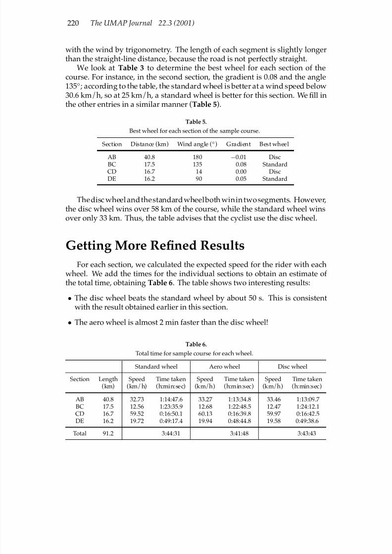
Getting More ReÞned Results

For each section, we calculated the expected speed for the rider with eachwheel. We add the times for the individual sections to obtain an estimate of the total time, obtaining Table 6. The table shows two interesting results:

• The disc wheel beats the standard wheel by about 50 s. This is consistentwith the result obtained earlier in this section.

• The aero wheel is almost 2 min faster than the disc wheel!

Table 6.

Total time for sample course for each wheel.

Standard wheel Aero wheel Disc wheel

Section Length Speed Time taken Speed Time taken Speed Time taken

(km) (km/h) (h:min:sec) (km/h) (h:min:sec) (km/h) (h:min:sec)

AB 40.8 32.73 1:14:47.6 33.27 1:13:34.8 33.46 1:13:09.7BC 17.5 12.56 1:23:35.9 12.68 1:22:48.5 12.47 1:24:12.1CD 16.7 59.52 0:16:50.1 60.13 0:16:39.8 59.97 0:16:42.5DE 16.2 19.72 0:49:17.4 19.94 0:48:44.8 19.58 0:49:38.6

Total 91.2 3:44:31 3:41:48 3:43:43

7/17/2019 UMAP 2001 vol. 22 No. 3



Validating the Model

Sensitivity Analysis

Does the table generated for one rider with a speciÞc set of physical at-

tributes apply to another rider, and if not, can the model easily be adjusted?To determine whether the same table could be used for different riders,

we varied one of the rider’s parameters, either power output, mass, or cross-sectional surface area, while keeping the others constant. In these analyses wefound that

• Changing any one or any combination of the parameters P , A , or M doesnot affect the basic pattern but slightly distorts (shifts, scales, or skews) it.

• Every rider-cycle combination would need its own chart for determiningwhich wheel to use at which speed.

Other Validation

We compared our model’s output to data available at Analytic Cycling[2001], which provides interactive forms. Our model’s output matched theiroutput almost exactly for all the different combinations of input parametersthat we used. Unfortunately, this site does not make provision for wind speedor angle, so this part of our model could not be compared.

We tested the model with a completely different set of parameters approx-imating a very powerful sports car (P = 300 kW, C d = 0.3 , A = 2.3 m2 ,M = 1100 kg). We kept the other parameters the same. Our model predicteda top speed of 320 km/h on a level road, which seemed very realistic.

Error Analysis

We were concerned about the disc wheel “islands” that showed up in ourgraphical output at wind speeds of 40–50 km/h, wind angles of 30◦–60◦ , andhighergradients(seeFigure3). They probablyaredue tothepeculiarbehaviourof disc wheels in crosswinds. Since we extrapolated the drag coef Þcient func-tion, we have no way of knowing whether this strange behaviour is realistic ornot.

Model Strengths

If a rider can obtain reasonably accurate course data (something that is notdif Þcult at all), then the rider can determine exactly what type of rear wheel touse for a race by referencing this information to a chart or computer.

7/17/2019 UMAP 2001 vol. 22 No. 3



The model has many parameters (air density, coef Þcients, rider mass, etc.)that can be adjusted to account for various situations.

It is easy to extend the model to include the front wheel of the bicycle.

Model WeaknessesWhen the angle of the wind with the cyclist changes, there are a number

of factors that inßuence the amount of drag that the cyclist experiences. Themost obvious is the changing surface area; a cyclist from the side presents a farlarger surface area to the wind than a cyclist heading into the wind.

Less obvious, but still a large contributing factor, is that the drag coef Þcientis a function of the shape of the object. A cyclist from the side is far lessstreamlined and has a higher drag coef Þcient.

Both these factors are extremely dif Þcult to model. The cross-sectional sur-face area of a complex three-dimensional shape could be the subject of a paper

on its own, and determining the drag coef Þcient of the same complex shapewould require empirical tests.

As a result, weignored these effects and assume that the dragcoef Þcientandcross-sectional surface area of the rider are the same for all directions. Strongcross-winds would cause too much rider instability to even consider using discwheels, so it would not really be necessary to investigate drag in such cases.

We also ignored the effects of the energy needed to overcome the rotationaland translational inertia for each wheel. We cannot comment on the effect of these forces, since we did not have time to implement these effects.

The model is only as accurate as the data used, and much of the available

data on wheel drag is, at best, dubious. Many wheel manufacturers exaggeratethe performance of their brands, while rival manufacturers quickly denouncetheir Þndings. Further, few data were available for yaw angles greater than30◦ , and we were forced to extrapolate, leading to a high degree of uncertainty.

Using the table requires speciÞc information about rider characteristics,some of which may be dif Þcult to obtain, such as the surface area of rider and bicycle.

Conclusion

Our model provides a good means for making an informed decision as towhich wheel to use in a particular situation, but it needs more accurate dataand reÞnement.

7/17/2019 UMAP 2001 vol. 22 No. 3



References

Analytic Cycling. 2001. http://www.analyticcycling.com .

Basis Systeme Netzwerk. 2001. Wheel aerodynamics. http://www.bsn.com .

BeaconsÞeld Cycling Club. 2001. Aero wheels under scrutiny.http://www.clubcycliste.com/english/archives/freewheel98/

freew498/f498aero.html .

Campagnola. 2001. http://www.campagnola.com .

Dragforcesinformulas. 2001. http://www.damopjinard.com/aero/formulas.htm .

Mavic cycles. 2001. http://www.mavic.com .

Tew, G.S., and A.T. Sayers. 1999. Aerodynamics of yawed racing cycle wheels. Journal of Wind Engineering and Industrial Aerodynamics 82: 209–221.

Acknowledgments

We would like to thank the Department of Applied Mathematics at Stel-lenbosch University for the generous use of their computing facilities and forcatering for us during the weekend of the competition.

7/17/2019 UMAP 2001 vol. 22 No. 3



7/17/2019 UMAP 2001 vol. 22 No. 3


Selection of a Bicycle Wheel Type 225

Selection of a Bicycle Wheel Type

Nicholas J. HowardZachariah R. Miller

Matthew R. AdamsUnited States Military AcademyWest Point, NY

Advisor: Donovan D. Phillips

Introduction

We present a model that compares the performance of various wheels over

a user-determined course. We approach the modeling problem by beginningwith Newton’s SecondLaw of Motion: The sum of the forces actingon an objectequals the mass of that object multiplied by its acceleration.

We identify the four principal forces that contribute to a cyclist’s motion:applied force, drag force, gravity, and rolling resistance. We further classifydrag force into three components: thecyclist andbicycle frame, thefrontwheel,and the rear wheel.

Drag force is dependent on a cyclist’s velocity, and the force of gravity isdependent on a cyclist’s position. Thus, our force equation is a function of cyclist position and cyclist velocity.

We can then arrange Newton’s Second Law to yield a second-order differ-

ential equation. Given position S , velocity dS/dt , acceleration d2S/dt2 , massm , and a force function F , the differential equation is

d2S

dt2 =

F

S, dS dt

m

.

To implement our model, we created a computer software program thatallows a user to input numerous pieces of data, including course layout, eleva-tion proÞle, wind, weather conditions, and cyclist characteristics. The softwareiterates the differential equation using the fourth-order Runge-Kutta method.The software reports the preferred wheel choice based on the data.

As a real-world application of our model, we analyze the 2000 OlympicCycling time-trial race. Over that course, a disk wheel provided a considerableadvantage over a spoked wheel.


7/17/2019 UMAP 2001 vol. 22 No. 3



Problem Analysis

We must determine whether a spoked wheel (lighter but less aerodynamic)or a disk wheel (more aerodynamic but heavier) is more power-ef Þcient. Thechoice depends on many factors, including the number and steepness of hills,

the weather, wind speed and direction, and type of competition.We are not striving to discover which wheel is best for all situations. To the

contrary, we are interested in which wheel outperforms other wheelsgiven spe-ciÞc conditions. Given accurate data concerning factors such as hills, weather,wind, and competition type, a good model will be able to determine and rec-ommend which wheel is preferred.

Our Approach

Wedetermineequationsforeachforcethatactsonthecyclistandthebicycle.These forcesare notconstant throughout a race. Forexample, airdrag increaseswith the square of velocity.

We apply Newton’s Second Law of Motion to the cyclist-bicycle system:The sum of the forces acting on an object equals mass of the object times itsacceleration. The sum of the forces is a function of both position on the courseandvelocity of thecyclist. Because theforces are different at differentpositions,the power required with a given type of wheel is also different. Our approachis to apply the same power to both types of wheels and determine how long ittakes to traverse the course. The wheel that allows the cyclist to complete thecourse in the shortest time requires less power, that is, is more power-ef Þcient.

A more comprehensive model would incorporate wind based upon a prob-abilistic function. However, to do so would be at odds with our goal: We wishto determine performance times for two types of wheels given a constant set of conditions. If we included probabilistic functions, differing performance timeswould be due to both wheel differences and random ßuctuations instead of just to wheel differences.

Let the position of the bicycle on the course be S with components S x , S y ,and S z . The second-order differential equation for acceleration is

d2S

dt2 =

F

S, dS dt

m ,

where d2S/dt2 is the acceleration, F (S, dS/dt) is the total force, and m is thetotal mass of the system.

We determine the time that it takes to complete a course by solving thisequation numerically.

7/17/2019 UMAP 2001 vol. 22 No. 3



Assumptions

• Weatherconditions(temperature, humidity, winddirection, andwindspeed)are uniform over thecourseandconstant throughout therace. Because windvariesover time, andterrain signiÞcantlychanges wind speed anddirection,

larger courses with greater variability in elevation are most affected by thisassumption. However, due to the unpredictability of the weather, a generalwind directionandspeed is probably themost detailed information to whichthe rider will have access.

• Both wheel types use the same tire.

• Turning does not signiÞcantly affect power ef Þciency of the wheel, speed of the rider, or acceleration of the rider.

• Based on the previous assumption, we assume that the bicycle moves in alinear path in 3-D space.

• The cyclist applies power according to the function that we develop in theModel Design section below, where we introduce other assumptions asso-ciated with developing this function.

• The drag coef Þcient for the rider plus bike frame is the same for all ridersand does not change as a function of yaw angle. The drag coef Þcient is 0.5and the cross sectional area is 0.5 m2 [Analytic Cycling 2001a].

• The wheels do not slip in any direction as they roll over the course.

• Other riders have no effect on the aerodynamic characteristics of the bike-

rider system. This means that we ignore the effects of drafting (which canreduce drag by up to 25%).

• The rider uses a conventional 36-spoke wheel on the front of the bike.

• The rotational moments of inertia for disc wheels and spoke wheels areapproximately 0.1000 kg-m2 and 0.0528 kg-m2 , respectively. In reality, thesemust be determined experimentally.

Model Design

We identify the forces that act on a bicycle and rider:

• The forward force that the rider applies with pedaling.

• Thedrag force that opposes themotionof thebicycle. Since weareconcernedwith analyzing wheel performance, we divide the total drag force into threecomponents:

7/17/2019 UMAP 2001 vol. 22 No. 3



– The drag force F f on the front wheel.

– The drag force F r on the rear wheel.

– The drag force F B on the bicycle frame and rider.

• The force of gravity F g that either opposes or aids motion due to the road

grade.

• The force of rolling resistance F rr due to the compression and deformationof air in the tires.

Because weassumethat the bicycle travels ina linearpath, weneedconsideronly components of these forces that act co-axially (i.e., parallel to the bicycle’sdirectionof movement). This will remain realistic solong astheassumptionthatthe wheels do not slip remains true, because the static frictional force betweenthe wheels and the ground prevents movement normal to the velocity.

Consequently, we do not need to treat the forces as vectors; we must note

only whether they aid or oppose the bike’s movement.

The Force that the Rider Applies

Theriderapplies a force tothepedals, whichthegearstranslateto thewheelsof the bicycle. Competitive bicycle racers generally shift gears to maintaina constant force on the pedals as well as a constant pedaling rate (cadence)whenever the sum of the other forces oppose the motion (i.e., going up a hillor into the wind) [Harris Cyclery 2001]. In other words, the cyclist attempts toexert constant power.

However, as therider moves downhill, gravity aids theeffort. As thebicyclegains speed, therider’s pedalingresults in a diminishedeffect on speed becausedrag forces increase with the square of speed. Eventually, at a speed vcutoff , therider ceases pedaling.

We model the power P a that the rider inputs as a function of speed vg:

P a =

0, if vg ≥ vcutoff ;

P avg, if vg < vcutoff ,

where P avg is the average power that the rider can sustain; its value varies fromrider to rider and with the type of race. Typical values range from 200 W forcasual riders to between 420–460 W for Olympic athletes on long-distance roadraces, to as much as 1500 W in sprint races [Seiler 2001].

If we assume that there is no energy lost in the translation of the power between the pedal and the wheel (i.e., in the gears), then by conservation of energy the power goes into either rotating the wheels or moving the bicycleforward:

P a = P w + P f , (1)

7/17/2019 UMAP 2001 vol. 22 No. 3



where P w is the power to rotate the wheels and P f is the power to drive the bicycle forward.

From elementary physics, the rotational kinetic energy of an object is 12Iω2 ,where I is the rotational moment of inertia and ω is the angular velocity of theobject. For the front and rear wheels, we have

K f = 12I f ω

2, K r = 12I rω2,

where I f and I r are the rotational moments of inertia of the front and rearwheels. The total rotational energy K T of the wheels is then

K T = K f + K r.

The powerdue tothe rotation of the object is the timederivativeof the rotationalenergy:

P w = dK T

dt =

d

dt 12I f ω2 + 1

2I rω2 = (I f + I r)ωω.

The angular velocity ω of an object equals its ground speed vg divided byits radius R , while its angular acceleration ω is a/R.

Substituting these into the above equation yields

P w = (I f + I r)vga

R2 .

Ifwesolveforthepower P a that pushesthebike forward, then divideboth sidesof (1) by vg , we obtain the applied force F A that pushes the bicycle forward:

P f

= P a −

P w

, F A

= P a

vg −(I f

+ I r

) a

R2.

The Drag Forces on the Bicycle

The drag force acting on an object moving through a ßuid is

F = 12CρAV 2,

where ρ is the density of the ßuid(air), A is thecross-sectional area of theobject,V is its velocity relative to the ßuid, and C is the coef Þcient of drag that must be determined experimentally.

Air density, which can have a signiÞcant effect on drag forces, dependson temperature, pressure, and humidity. Pressure depends on altitude andweather. Most baseball fans can attest to the signiÞcant affects of air density ondrag forces: Baseballs carry much farther in Coors Field in Denver, Colorado, because the high altitude leads to a low pressure, which means that the airdensity is less as well.

We consider all of these factors that affect air density in our model, viacalculations in the Appendix [EDITOR’S NOTE: We omit the appendix.]. The

7/17/2019 UMAP 2001 vol. 22 No. 3



most important aspect is that the air density is a function of the bike’s elevation,S z . The bike’s acceleration d2S/dt2 depends on the drag forces, which dependon air density, which depends on the bike’s position. This means that thedifferential equation that we develop will be second-order, because the secondderivative of position depends on the position.

The Movement of the Air and Bicycle

The air through which the bicycle moves is not stagnant—wind blowingover the course has a signiÞcant effect. We represent the wind as a vector Þeld V A with a magnitude and direction that are uniform over the racecourse andconstant for the duration of the race.

The cyclist’s speed over the ground is vg; thus, the velocity is vgu , where uis a unit vector in the bicycle’s direction of movement. We now consider theair’s velocity relative to the bicycle instead of the bicycle’s velocity relative to

the air, because this is an easier way of thinking about the problem and themagnitudes of these two velocities are equal. Since the bike’s velocity over theground is vgu , the air’s velocity relative to the bike due to the bike’s motion is−vgu.

The total velocity of the air moving relative to the bike is a function of two

motions: the air’s movement relative to the ground in the form of wind, V A ,and the air’s movement relative to the bike due to the bike’s movementover theground,−vgu , where we use the hat over u to denote that u is a unit vector. Thetotal speed is then the magnitude of the sum of these two velocities (Figure 1),

vT =

V A

−vgu

.

Figure 1. Components of total air velocity.

The yaw angle θ is the angle between the bicycle’s axis of movement and

the air direction, which weÞnd from the dot product,a· b = a b cos θ , where

7/17/2019 UMAP 2001 vol. 22 No. 3



θ is the angle between the vectors. We have

−vgu · ( V A − vgu) = vg V A − vgu cos θ,

θ = arccos−vgu · ( V A − vgu

vg

V A−

vgu

.

The bicycle’s aerodynamic characteristics, and thus the drag forces, changewith θ. Furthermore, because the bicycle does not always head into the wind,the overall drag force has components both normal and axial to the rider’s path.We assume that the normal component is negligible and consider only the axialcomponent (the component parallel to the cycle’s axis of travel).

The Wheels

The axial drag force on the wheels largely depends on the yaw angle of

the air moving past them and must be calculated experimentally for differenttypes of wheels. For experimental results, we rely on Greenwell et al. [1995],who used a wind tunnel to determine the axial drag coef Þcient at different yawangles for various commercially available wheels.

For each type ofwheel, weplotted axial dragcoef Þcientvs.yawangle. Fromthe plots, we constructed a polynomial regression of axial drag coef Þcients asa function of the yaw angle. Greenwell et al. considered the reference cross-sectional area of each wheel S ref to be the total side cross-sectional area of thewheel,

S ref = πR2.

Thus, the effects of the cross-sectional area changing with yaw angle are in-cluded in the axial drag coef Þcient. Consequently, to use their results, we mustuse the same reference area. The axial drag force on the front wheel is then

F f = K W C F v2T ,

where K W = 12ρS ref and C F is the axial drag coef Þcient of the front wheel at

yaw angle θ.An interesting result of Greenwell et al. is that drag forces on the rear wheel

are generally reduced by about 25% due to aerodynamic effects of the seat tube.This means that the axial drag force on the rear wheel is

F R = (0.75)K W C Rv2T ,

where C F is the axial drag coef Þcient of the rear wheel at yaw angle θ.

The Bicycle Frame and RiderUnfortunately, we were not able to obtain data relating the drag coef Þcient

of the rider and frame to the yaw angle, so we could consider only the effectsof the component of the wind that is parallel to the bicycle’s velocity.

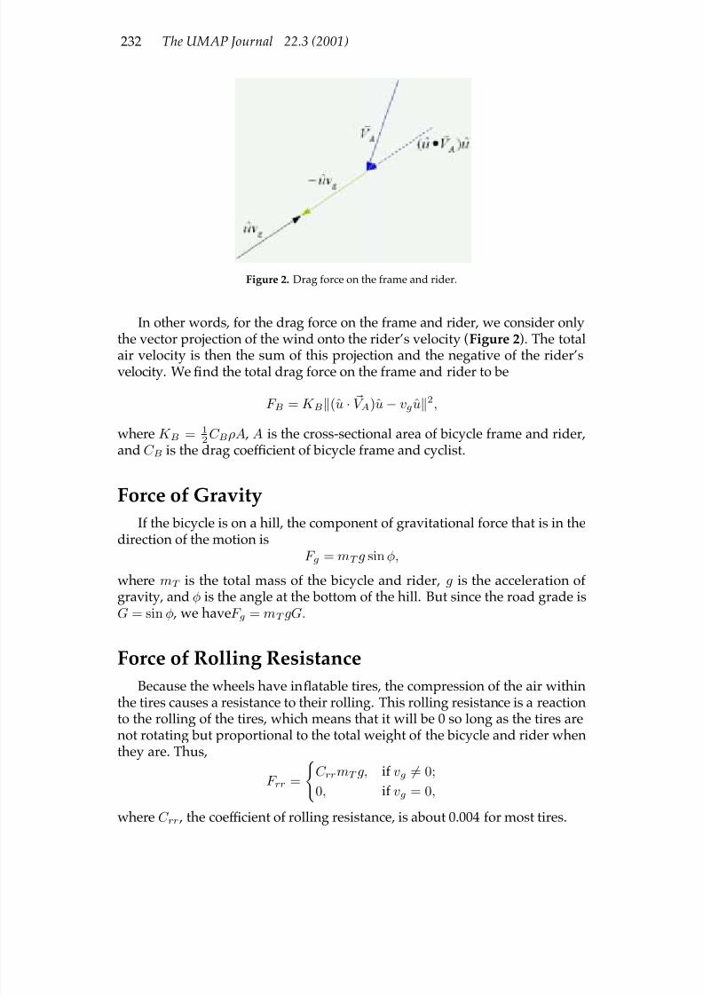
7/17/2019 UMAP 2001 vol. 22 No. 3



Figure 2. Drag force on the frame and rider.

In other words, for the drag force on the frame and rider, we consider onlythe vector projection of the wind onto the rider’s velocity (Figure 2). The totalair velocity is then the sum of this projection and the negative of the rider’svelocity. We Þnd the total drag force on the frame and rider to be

F B = K B(u · V A)u− vgu2,

where K B = 12C BρA , A is the cross-sectional area of bicycle frame and rider,

and C B is the drag coef Þcient of bicycle frame and cyclist.

Force of Gravity

If the bicycle is on a hill, the component of gravitational force that is in thedirection of the motion is

F g = mT g sin φ,

where mT is the total mass of the bicycle and rider, g is the acceleration of gravity, and φ is the angle at the bottom of the hill. But since the road grade isG = sin φ , we haveF g = mT gG.

Force of Rolling Resistance

Because the wheels have inßatable tires, the compression of the air withinthe tires causes a resistance to their rolling. This rolling resistance is a reactionto the rolling of the tires, which means that it will be 0 so long as the tires arenot rotating but proportional to the total weight of the bicycle and rider whenthey are. Thus,

F rr =

C rrmT g, if vg = 0;

0, if vg = 0,

where C rr , the coef Þcient of rolling resistance, is about 0.004 for most tires.

7/17/2019 UMAP 2001 vol. 22 No. 3



Summing the Forces

We sum the forces that act in the model:

F A − F B − F f − F r − F g − F RR = mT a, (2)

where

F A = P avg− (I f + I r)

a

R2 (forward force that rider exerts),

F B = K B(u · V A)u− vgu)2 (drag force on bike frame and rider),

F F = K W C F v2T (drag force on front wheel),

F R = 0.75K W C Rv2T (drag force on rear wheel),

F g = mT gG (force of gravity),

F rr = C rrmT g if vg = 0 , 0 if vg = 0 (force of rolling resistance).

The forward force of the rider depends on acceleration. Since we want tohave all the acceleration terms together, we Þrst group them:

P avg− (I f + I r)

a

R2

− F B − F f − F r − F g − F RR = mT a,

P avg− F B − F f − F r − F g − F RR = a

mT +

I f + I rR2

.

Substituting the other forces into (2) , we obtain

P avg−K B(u· V A)u−vgu2−K W C F v

2T −0.75K W C Rv2T −mT gG =

mT +

I f + I rR2

a.

Solving for a , we Þnd the second-order differential equation

a = d2S

dt2 =

P avg−K B(u · V A)u− vgu2 −K W C F v

2T − 0.75K W C Rv2T − mT gG

mT + I f + I r

R2

.

Completing the Model

This differential equationistoocomplicated tosolveanalytically, sowesolveit numerically using a fourth-order Runge-Kutta (RK4) approximation method[Burden and Faires 1997]. This method is generally more accurate than othernumerical approximation methods such as Euler’s method, especially at pointsfarther away from the start point.

7/17/2019 UMAP 2001 vol. 22 No. 3



To make the approximation, we Þrst deÞne acceleration based on time t ,position (elevation S z), and speed vg:

a = a(t, S z, vg)

The RK4 method uses a weighted approximation of the acceleration at agiven time tk with speed vgk to determine the speed at some time tk+1 in thefuture, where tk+1 = tk + h , with h the time-step size.

(vg)k+1 = (vg) + 1

6 h (W K 1 + 2W K 2 + 2W K 3 + W K 4) ,

where

W K 1 = a(tk, vgk),

W K 2 = a

tk + h

2 , vk + hW K1

2 ,

W K 3 = a

tk + h

2 , vk + hW K2

2

,W K 4 = a(tk + h, vk + hW K 3).

As with any numerical approximation method, we must know the initial speedvg0 . Then, with the velocity computed at a given time, we calculate the positionof the bike at time tk+1 as

S k+1 = S k + h(vg)ku

from the initial position of the bike S 0. Again, because we consider only axialforces acting on the bike and ignore turning, we can model only a bike moving

ina straight line; thismeans that u , the unit vector in the directionof the velocity,is constant.

Model Validation

To validate our model, we developed a computer program to simulatetraversal of a course (see screen display in Figure 3). We inputted a map of the2000 Olympic Games time-trial course [NBC Olympics 2000a]. The prevailingwind speed and direction for Sydney on 27 September 2000 (the day of theOlympic Þnals for the road race) was 10 m/s at 315◦ [Analytic Cycling 2001].We assume that the winner would maintain an average power of 450 W.

Using our model, we calculated that cyclists would complete 15 laps of the15.3 km course in a time between 5 h 18 min and 5 h 47 min (depending onwhich wheel is used). In Sydney that day, Jan Ullrich of Germany won the racein a time of 5 h 29 min. As this result falls within the range of predicted values,we believe that our model is relatively accurate.

However, to test truly the validity of the model, we would need to ex-periment with various riders and wheel types for which we know the drag

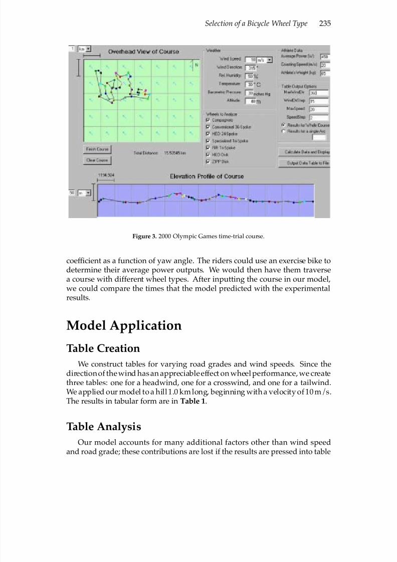
7/17/2019 UMAP 2001 vol. 22 No. 3



Figure 3. 2000 Olympic Games time-trial course.

coef Þcient as a function of yaw angle. The riders could use an exercise bike todetermine their average power outputs. We would then have them traversea course with different wheel types. After inputting the course in our model,we could compare the times that the model predicted with the experimental

results.

Model Application

Table Creation

We construct tables for varying road grades and wind speeds. Since thedirectionof thewind hasan appreciableeffect on wheel performance, we createthree tables: one for a headwind, one for a crosswind, and one for a tailwind.

We applied our model to a hill 1.0 kmlong, beginning with a velocity of 10 m/s.The results in tabular form are in Table 1.

Table Analysis

Our model accounts for many additional factors other than wind speedand road grade; these contributions are lost if the results are pressed into table

7/17/2019 UMAP 2001 vol. 22 No. 3



Table 1.

Preferred wheel type for a hill 1.0 km long and starting speed 10 m/s.

7/17/2019 UMAP 2001 vol. 22 No. 3



form. Additionally, cycling races generally do not consist of one large hill of auniform grade; there are typically many turns, hills, and valleys.

As a result, we recommend against using the tables that we provide! Oursoftware implementation of the model allows the entry of all factors relating tothe course that affect wheel choice.

Typically, course layout and elevation proÞle are available well in advanceof a cycling race. We recommend that users of our software input the courseand run multiple scenarios based on varying wind speeds and directions.

Results and Conclusions

We analyzed 7 different wheels: 5 spoked (Compagnolo, Conventional 36-Spoke, HED 24-Spoke, Specialized Tri-Spoke, and FIR Tri-Spoke) and 2 disc(HED Disc and ZIPP Disc). We chose these wheels because we could Þnddata relating the drag coef Þcients to the yaw angle of the air. After running

our model over varying courses and conditions, we came to some interestingconclusions, which mesh well with what intuition would suggest.

Crosswinds

In crosswinds, disc wheels dramatically outperform spoked wheels , since the dragcoef Þcients for disc wheels decreases sharply as the yaw angle increases. Asyaw angle increases to around 20◦ , drag coef Þcients for disc wheels drop dra-matically. For the HED Disc, the drag coef Þcients actually become negative atlarger yaw angles, indicating that the wheel acts like a sail and helps propel

the cycle forward instead of slowing it down! The ZIPP Disc drag coef Þcientsdo not become negative but drop very close to zero at larger yaw angles. Con-sequently, the difference in speed between discs and spokes in a crosswind issigniÞcant. If a course has a strong crosswind (greater than 20 mph), then adisc wheel can make time differences on the order of 20% or more. However,even in a light crosswind, the two disc wheels that we analyzed outperformed everyspoked wheel.

Direct Head and Tail Winds

In direct head and tail winds, spoked wheels slightly outperform disc wheels , be-cause both types have similar drag coef Þcients at small yaw angles and spokedwheels are lighter.

Spoked wheels generally outperform disc wheels when going uphill in theabsence of wind, because they are lighter, whereas disk wheels outperformspoked wheels when going downhill, because they are heavier. When thereis a head wind or a tail wind when going up a hill, spokes generally stilloutperform discs; however, the introduction of any cross wind with a yaw

7/17/2019 UMAP 2001 vol. 22 No. 3



angle much greater than 15◦ or 20◦ causes the smaller disc drag coef Þcients tooutweigh the mass differences. This means that disc wheels are more ef Þcientthan spoked wheels.

Long RacesIn long races, disc wheelsgenerallyoutperformspokedwheels , becausethe smaller

drag forces on the disc have a more signiÞcant effect on overall performance.Generally, in a race of any length much over 5 km, discs are more ef Þcient, because the wind acts on them for longer amounts of time than in short races,which means that aerodynamic characteristics are more important than massdifferences.

Short Races

In short races, where acceleration is more important, the spoked wheels,with their smaller masses and moments of inertia, outperform the disc wheels.

Strengths of the Model

Robustness. We derive our model from basic physical relationships and limitour use of assumptions. In every case where an assumption is required, wesubstantiate it with evidence and reasoning that illustrates why the assump-tion is valid.

Grounded in theory and research. We constructed our model based on boththeory (Newton’s second law) and research (Greenwell et al. [1995]).

Ease of use. Although the physical concepts behind our model are relativelysimple to understand, the mathematical derivations and calculations aredif Þcult to perform. We created a user-friendly computer program with agraphical interface that allows anyone with a basic knowledge of computersto input the required data. The program performs the mathematical calcu-lations and reports the preferred wheel choice, along with calculated stagetimes for the race.

Weaknesses of the Model

Representing the course. We represent the course as a sequence of points inthree-dimensional space, with the path from point to point represented by astraight line. This is not an accurate representation of any course; the traver-sal of hills, valleys, and curves all create nonlinear movement. Accuracy

7/17/2019 UMAP 2001 vol. 22 No. 3



could be increased through a detailed entering of the course with a largernumber of location nodes.

Approximation of wheel drag data. Greenwell et al. [1995] reported data foryaw angle 0◦ through 60◦ only in 7.5◦ increments. We developed interpo-lating polynomials through this range. We would conduct further tests atvarious yaw angles.

References

Analytic Cycling. 2001a. Wind on rider. http://www.analyticcycling.com/DiffEqWindCourse_Disc.html . Accessed 10 February 2001.

. 2001b. Forces source input. http://www.analyticcycling.com/ForcesSource_Input.html . Accessed 10 February 2001.

Burden, Richard L., and Douglas Faires. 1997. Numerical Analysis. 6th ed. NewYork: Brooks/Cole.

Greenwell, D., N. Wood, E. Bridge, and R. Addy. 1995. Aerodynamic charac-teristics of low-drag bicycle wheels. Aeronautical Journal 99 (March 1995):109–120.

HarrisCyclery. 2001. Bicycle glossary. http://www.sheldonbrown.com/gloss_ca-m.html#cadence . Accessed 10 February 2001.

NBCOlympics. 2000a. Individualtimetrial. http://sydney2000.nbcolympics.com/features/cy/2000/09/cy_feat_roadmap/cy_roadmap_01.html . Ac-

cessed 11 February 2001.. 2000b. Men’s road race results. http://sydney2000.nbcolympics.

com/results/oly/cy/cym012.html?event=cym012100o.js . Accessed 11February 2001.

Palmer, Chad. 2001. Virtual temperature and humidity. USA Today. http://www.usatoday.com/weather/wvirtual.htm . Accessed 10 February 2001.

Seiler, Stephen. 2001. MAPP Questions and Answers Page. Masters AthletePhysiology and Performance. http://home.hia.no/~stephens/qanda.htm . Accessed 10 February 2001.

7/17/2019 UMAP 2001 vol. 22 No. 3



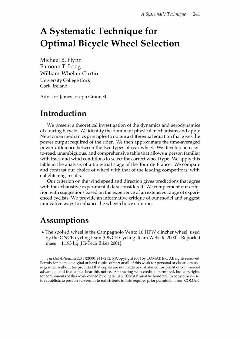
7/17/2019 UMAP 2001 vol. 22 No. 3


A Systematic Technique 241

A Systematic Technique for

Optimal Bicycle Wheel Selection

Michael B. FlynnEamonn T. LongWilliam Whelan-CurtinUniversity College Cork Cork, Ireland

Advisor: James Joseph Grannell

Introduction

We present a theoretical investigation of the dynamics and aerodynamicsof a racing bicycle. We identify the dominant physical mechanisms and applyNewtonian mechanics principles to obtain a differential equation that gives thepower output required of the rider. We then approximate the time-averagedpower difference between the two types of rear wheel. We develop an easy-to-read, unambiguous, and comprehensive table that allows a person familiarwith track and wind conditions to select the correct wheel type. We apply thistable in the analysis of a time-trial stage of the Tour de France. We compareand contrast our choice of wheel with that of the leading competitors, withenlightening results.

Our criterion on the wind speed and direction gives predictions that agreewith the exhaustive experimental data considered. We complement our crite-rion with suggestions based on the experience of an extensive range of experi-enced cyclists. We provide an informative critique of our model and suggestinnovative ways to enhance the wheel-choice criterion.

Assumptions

• The spoked wheel is the Campagnolo Vento 16 HPW clincher wheel, used

by the ONCE cycling team [ONCE Cycling Team Website 2000]. Reportedmass = 1.193 kg [Hi-Tech Bikes 2001].


7/17/2019 UMAP 2001 vol. 22 No. 3



Table 1.

Model Inputs and Symbols.

s distance over which the average power is calculatedk road gradeu initial speed of the rider before any inclinecr coef Þcient of air drag for the bike and the rider frameAr cross-sectional area of bike and rider frameρ air densitym(spk) mass of spoked rear wheelm(sld) mass of disc rear wheelcr coef Þcient of rolling resistanceg 9.81m/s2 acceleration due to gravitycfw drag coef Þcient of front wheelcrw(sld) drag coef Þcient of solid wheelcrw(spk) drag coef Þcient of spoked wheelrrw radius of rear wheelµ constant of decelerationφ angle of wind with respect to direction of bike (degrees)vf speed of the wind with respect to the cyclist

I rw moment of inertia of the rear wheelI fw moment of inertia of the front wheelvw wind speedν kinematic viscosity of air

• The density and pressure of the air across the bike are essentially constant.(See Appendix. [EDITOR’S NOTE: We omit the Appendix.])

• For most of the journey, the bike travels in a straight line (±10%). This isreasonable, since cyclists avoid turning as much as possible and they havea wide enough road to achieve a straight line.

• The solid wheel is taken to be the HED disc tubular freewheel, the solidwheel of choice in the Tour de France. Reported mass = 1.229 kg [Hi-TechBikes 2001].

• The dragcoef Þcientsofbothwheelsare independent of the windspeed intherange of raceable weather conditions and vary signiÞcantly with the relativedirection of the wind [Flanagan 1996].

• The drag area of a typical crouched racer is 0.3 m2 [Compton 1998].

• The radius of the wheel is 35 cm [Compton 1998].

• Theef Þciencyof thedrive train is essentially100%, reasonable for elite racing bikes [Pivit 2001].

• The coef Þcient of rolling resistance between road and wheel rubber is 0.007[Privit 2001].

• The moment of inertia of a bicycle wheel about an axis through its centreandperpendicular to the plane of the wheel is I = 1

9mr2 , where m is the mass

7/17/2019 UMAP 2001 vol. 22 No. 3



of the wheel and r is the radius. This agrees with empirical data [Compton1998].

• The deceleration to terminal speed on a uniform incline is constant to within±2%.

• The terminal speed on a uniform incline is reached at 100 m up the incline.

• The deceleration of a rider on a slope is proportional to the gradient of theslope (given in the problem statement).

• The power is averaged over 100 m of acceleration, where the accelerationis that calculated in the Appendix. This power is used in determining thewind speed criterion for solid wheels.

• All of the drag due to the rider and bike frame is due to the rider cross-sectional area, since the area of the rider is much greater.

• The rolling resistance crrmg is the same for the solid wheel as for the spokedwheel. Thetiressurroundingthewheelsareidenticalandthemassdifference between the wheels is only about 0.1% of the overall mass of the bike plusrider.

The Wind Speed Criterion

We have from Newton’s Second Law that F = ma , where F is the forceacting the object, m is its mass, and a is its net acceleration. For the bicycle, the

force equation can be written as follows:Force applied by rider = Retarding Forces + ma + rotational acceleration,

where m is the mass of the rider-bike system. The retarding forces consist of

• the drag due to the bike frame and the rider,

• the drag due to the individual wheels,

• the friction due to the motion of the wheels in the air, and

• the rolling resistance of the wheels on the surface.

7/17/2019 UMAP 2001 vol. 22 No. 3



The formulas for these torques and forces are

drag force of bike frame and rider =cwAρv2f

2 ,

drag force due to front wheel =

cfwAρv2f

2 ,

drag force due to rear wheel =crwAρv2f

2 ,

frictional torque = 0.616πρω3/2ν 1/2r4,mr + mb + mfw +

I fwr2

+ mrw + I rw

r2

a = Resultant Force.

With this in mind, the power is averaged. The criterion on the wind speedvw becomes:

vw >

mrw(sld)−mrw(spk)(σspk − σsld)

+

γ s

2 − λ

s + γ

s,

where σ , λ , and γ are as given in the Appendix. If the quantity on the left sideis not positive, then the solid wheel is always best. The quantity σ is effectivelyan aerodynamic term, whereas γ and λ can be thought of as representing theacceleration, and time of acceleration respectively. Note that γ is dependent onthe wind direction φ.

The Minimum Wind Speed TableTable 2 gives the wind speed below which the power for the spoked wheel

is less, for various rider speeds. A 0 means that for any nonzero wind speed,the solid wheel requires less power; ∞ means that the rider will not be able tocontinue up the slope for 100 m.

Course Example

Time-trial course: Stage 1 , Tour de France 2000 (Figure 1): A 16.5 km circuit

starting at the Futuroscope building in Chassenuil-du-Poitou, France [Tourde France 2000].

Modeling the course: The course is modeled by a quadrilateral. This is a faith-ful representation of the course [CNN/Sports Illustrated Website 2000]. Thiscourse is predominantly level (Figure 2) save for a 1 km climb at a gradientof 3.7%. This climb is treated as the crucial feature of the time trial course,insofar as wheel choice is concerned.

7/17/2019 UMAP 2001 vol. 22 No. 3



Table 2.

Wind speed (in m/s) below which the power for the spoked wheel is less.

a.

Rider speed of 10 m/s.

Wind direction 180◦ 173◦ 165◦ 150◦ 135◦

Road Grade0.00 16 0 0 0 00.01 23 0 0 0 00.02 29 1 0 0 30.03 34 3 0 0 50.04 39 4 0 0 70.05 43 6 1 0 80.06 48 7 3 0 100.07 51 8 4 0 110.08 55 10 5 1 130.09 59 11 6 2 14

0.10 ∞ ∞ ∞ 3 ∞

b.

Rider speed of 12.5 m/s.

Wind direction 180◦ 173◦ 165◦ 150◦ 135◦

Road Grade0.00 13 0 0 0 00.01 21 0 0 0 00.02 25 0 0 0 00.03 26 0 0 0 20.04 32 2 0 0 3

0.05 36 3 0 0 50.06 41 4 0 1 70.07 45 5 0 2 80.08 48 7 1 3 100.09 52 8 2 4 110.10 59 9 3 5 12

c.

Rider speed of 14 m/s.

Wind direction 180◦ 173◦ 165◦ 150◦ 135◦

Road Grade

0.00 12 0 0 0 00.01 19 0 0 0 00.02 25 0 0 0 00.03 30 0 0 0 00.04 35 0 0 0 10.05 39 1 0 0 30.06 43 3 0 0 50.07 47 4 0 0 60.08 50 5 0 1 80.09 54 6 0 2 90.10 57 7 1 3 10

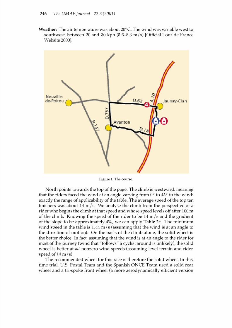
7/17/2019 UMAP 2001 vol. 22 No. 3



Weather: The air temperature was about 20◦C. The wind was variable west tosouthwest, between 20 and 30 kph (5.6–8.3 m/s) [Of Þcial Tour de FranceWebsite 2000].

Figure 1. The course.

North points towards the top of the page. The climb is westward, meaningthat the riders faced the wind at an angle varying from 0◦ to 45◦ to the wind:exactly the range of applicability of the table. The average speed of the top tenÞnishers was about 14 m/s. We analyse the climb from the perspective of arider who begins the climb at that speed and whose speed levels off after 100 mof the climb. Knowing the speed of the rider to be 14 m/s and the gradientof the slope to be approximately 4% , we can apply Table 2c. The minimumwind speed in the table is 1.44 m/s (assuming that the wind is at an angle tothe direction of motion). On the basis of the climb alone, the solid wheel isthe better choice. In fact, assuming that the wind is at an angle to the rider formost of the journey (wind that “follows” a cyclist around is unlikely), the solidwheel is better at all nonzero wind speeds (assuming level terrain and riderspeed of 14 m/s).

The recommended wheel for this race is therefore the solid wheel. In thistime trial, U.S. Postal Team and the Spanish ONCE Team used a solid rearwheel and a tri-spoke front wheel (a more aerodynamically ef Þcient version

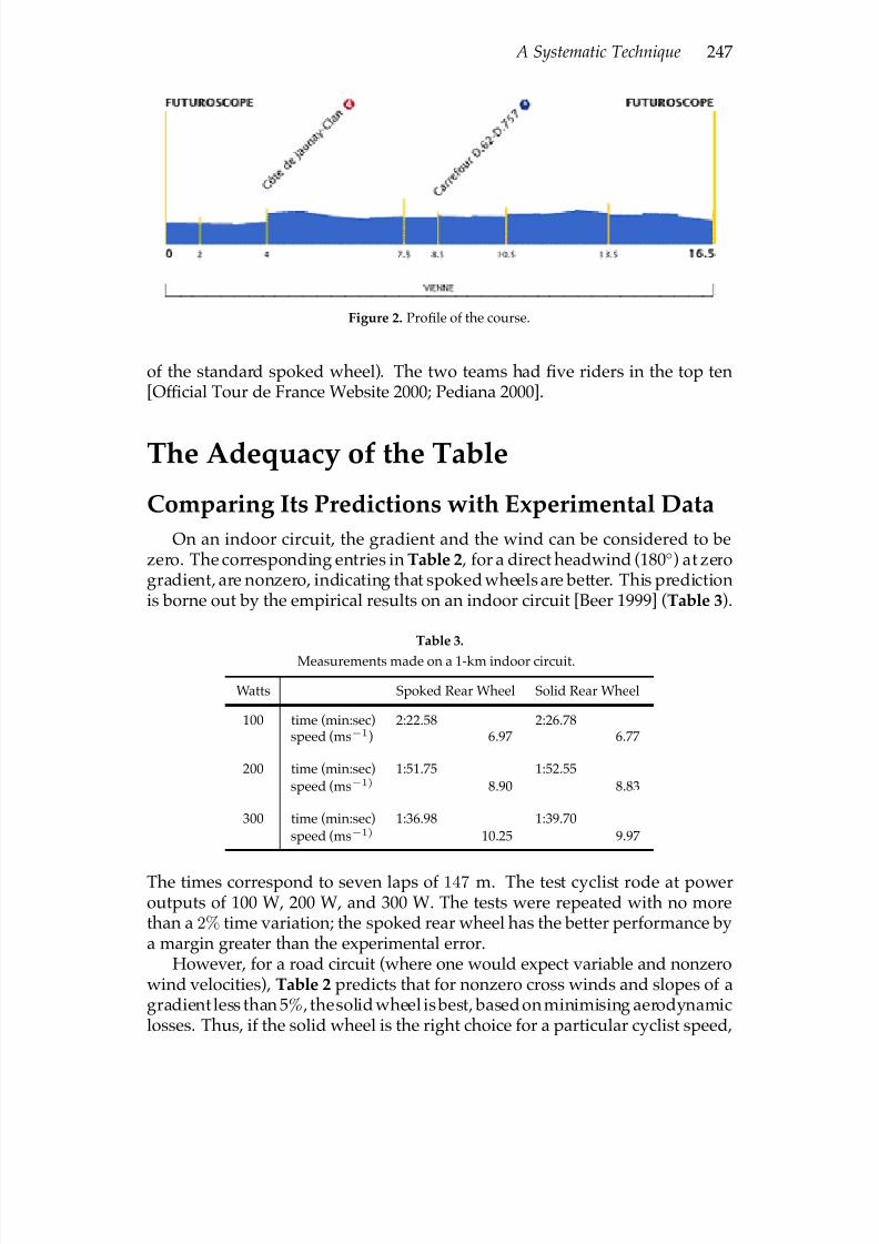
7/17/2019 UMAP 2001 vol. 22 No. 3



Figure 2. ProÞle of the course.

of the standard spoked wheel). The two teams had Þve riders in the top ten[Of Þcial Tour de France Website 2000; Pediana 2000].

The Adequacy of the Table

Comparing Its Predictions with Experimental Data

On an indoor circuit, the gradient and the wind can be considered to bezero. The corresponding entries in Table 2 , for a direct headwind (180◦) at zerogradient, are nonzero, indicating that spokedwheels are better. This predictionis borne out by the empirical results on an indoor circuit [Beer 1999] (Table 3).

Table 3.

Measurements made on a 1-km indoor circuit.

Watts Spoked Rear Wheel Solid Rear Wheel

100 time (min:sec) 2:22.58 2:26.78speed (ms−1) 6.97 6.77



The times correspond to seven laps of 147 m. The test cyclist rode at poweroutputs of 100 W, 200 W, and 300 W. The tests were repeated with no morethan a 2% time variation; the spoked rear wheel has the better performance bya margin greater than the experimental error.

However, for a road circuit (where one would expect variable and nonzerowind velocities), Table 2 predicts that for nonzero cross winds and slopes of agradient less than 5%,thesolidwheel isbest, basedon minimising aerodynamiclosses. Thus, if the solid wheel is the right choice for a particular cyclist speed,

7/17/2019 UMAP 2001 vol. 22 No. 3



then the solid wheel choice is valid for all greater cyclist speeds, given the sameatmospheric conditions. Experimental data in Table 4 back up this claim.

Table 4.

Measurements made on a 7.2-km road circuit.

Watts Spoked Rear Wheel Solid Rear Wheel

200 time (min:sec) 15:22 13:53speed (ms−1) 7.81 8.63

The circuit consisted of a 7.2-km looped course of rolling hills (gradient< 5%) with varying wind conditions (nonzero wind speeds, unlike the indoortrack). The power output of the cyclist was approximately 200 W. The testswererepeated with no morethan a 2.3% time variation. For theroad circuit, thesolid rear wheel is thebetterchoice (againby more than theexperimentalerror).According to the appropriate table, the solid rear wheel is the more ef Þcient

for most of the conditions that were encountered. Thus, the predictions of themodel are once more conÞrmed.

Additional Factors Not Considered by the Table

Stability of the bike: Stability is a major factor in cycling. A cyclist wants toconcentrate on putting the maximum possible power through the pedals. If the bicycle is unstable, the jerking of the handlebars in response to suddengusts of wind will be very disruptive. In general, bicycles with standardspoked wheels front and rear are the least affected by changing crosswinds,

but bikes with solid wheels are fastest. A solid front wheel can increase therider’s pedaling wattage by 20% to 30%, but it removes all the bicycle’s self-centering effects, making for a dif Þcult ride. A solid rear wheel has similar but milder effects [Cobb 2000].

Turning radius: This factor is important if the course contains many turns orif maneuvering in response to other riders is necessary. A greater turningradius loses time at each turn, where more maneuverable riders may over-take.

Rider comfort: The solid wheel also creates the problem of rider comfort. As it

has no spokes, it cannotß

ex to absorb any shocks due to irregularities of theroad surface. Towards the end of a long race, a rider’s concentration may be impaired due to the resulting discomfort, causing a drop in performance[Bicycle Encyclopedia 2000].

Very few cyclists ride with two solid wheels (1out of 177 in the time trial thatwe studied), despite the aerodynamic superiority—steering problems negatethe gain. Similarly, we have shown the superiority of the solid rear wheel inrace conditions, yet in the long-distance (150+ km) stages of the Tour de France,

7/17/2019 UMAP 2001 vol. 22 No. 3



all riders use spoked wheels: Solid wheels have insuf Þcient maneuverabilityand steering problems cause mental fatigue near the end of the stage.

Thus, the directeur sportif should consider the length of the race, the windconditions, and the quality of the road surface in making the decision.

Error Analysis

The error was determined by calculating the differential.The wind direction may vary considerably over a given course due to local

effects (e.g., buildings, trees). We chose an error of 10% for cfw(φ) and crw(φ).Air density can usually be determined to a high accuracy but varies by

location. Therefore, we chose a 1% error, since the necessary equipment isunlikely to be available to the directeur sportif at the time of the race.

Using a wind tunnel, drag coef Þcients can be determined to a very high pre-cision (to within 0.02kg); but variables such as pedaling speed, wheel rotation,

and rider posture introduce inaccuracies that cannot be easily determined. Themain dif Þculty is that the ßowÞeld about a rider in a wind tunnel is not ergodic,primarily as a result of airßow irregularities caused by pedaling. Therefore,we chose an error of 3% for cr [Flanagan 1996].

For each rider/bicycle combination, the directeur sportif should determinethe appropriate masses and dimensions. We assume that they can be deter-mined to a high degree of accuracy (∼ 0.1%) with the exception of the rider’scross section, in which we take an error of 2%. From error analysis in theAppendix , we Þnd

vw

vw = 16%.

Strengths and Weaknesses

Our model clearly and concisely states which wheel should be used underthe various conditions. The model is based on equations that are suf Þcientlyversatile so that further factors pertaining to a particular situation may be in-cluded as required, without any need to construct new equations.

We could not verify the model experimentally under conditions of the highpower output of elite cyclists. However, in data available for various lesserpower outputs, we could not discern any noticeable trends in time differential between the different wheels with respect to increasing power.

Our model does not contain a quantitative analysis of the wind speedsat which the solid wheel is unacceptably unstable. However, this questiondepends largely on the abilities and preferences of each individual rider andrequires detailed local information about road conditions and wind variability.

No data were available regarding the coef Þcients of drag in a tail wind.However, since the cyclist (∼ 15 m/s) in general travels faster than the wind

7/17/2019 UMAP 2001 vol. 22 No. 3



(race conditions < 10 m/s), only the crosswind effects are important, and theseare adequately handled in the tables.

The major weakness of the model is assuming that the rider’s speed doesnot differ much from the rider’s average speed over the duration of the race.Moreover, we couldÞnd no evidence to support theproblem’s assumption that

a rider reaches terminal velocity after 100 m of a slope.

Conclusion

• When there is a head wind, the spoked wheel is better. If the course is ßat,the solid wheel is better for strong winds; however, the wind (particularly if gusting) may cause instability problems.

• When the wind is not weak (> 5 m/s) and strikes the wheel at an angle,the solid wheel is nearly always better. Even a small component of wind

perpendicular to the rider direction makes the solid wheel the better choice.

• If the circuit has many tight turns or involves riding in close company withother cyclists, the solid wheel’s lack of maneuverability dictates the spokedwheel; otherwise, the risk of an accident and injury is unacceptable.

• The region of superiority of the solid wheel increases with rider speed. Sincethepowerrequired to overcome airresistance goes as thecube of thevelocity,the aerodynamic savings of the solid wheel become more important withhigher speed.

ReferencesBeer, Joe. 1999. Cycling Plus (January 1999) 19–22.Is a racing recumbent really

faster than an aero trial bike or a quality road bike? http://http://www.necj.nj.nec.com/homepages/sandiway/bike/festina/cplus.html .

The Bicycle Encyclopedia. 2001. http://my.voyager.net/older/bcwebsite/test/w/wheelset.htm .

Chow, Chuen-Yen. 1979. AnIntroduction to Computational FluidMechanics. NewYork: Wiley.

CNN/Sports Illustrated Website. 2001. http://sportsillustrated.cnn.com/cycling/2000/tour_de_france/stages/1/ .

Coast, J.R. 1996. Whatdetermines the optimal cadence? Cycling Science (Spring1996) http://www.bsn.com/cycling/articles/ .

Cobb, John. 2000. Steering stability explained. http://www.bicyclesports.com/technical/aerodynamics .

7/17/2019 UMAP 2001 vol. 22 No. 3



Cochran, W.G. 1934. Proceedings of the Cambridge Philosophical Society 30: 365ff.

Compton, Tom. 1998. Performance and wheel concepts.http://www.analyticcycling.com .

Flanagan, Michael J. 1996. Considerations for data quality and uncertainty in

testing of bicycle aerodynamics. Cycling Science (Fall 1996).http://www.bsn.com/cycling/articles .

Douglas, J.F. 1975. Solutions of Problems in Fluid Mechanics. Bath, England:Pitman Press.

, J.M. Gasiorek, and J.A. Swaf Þeld. 1979. Fluid Mechanics. Bath,England: Pitman Press.

Giant Manufacturing Co., Ltd. 2001. http://www.giant-bicycle.com .

Hi-Tech Bikes. 2001. http://www.hi-techbikes.com/ .

Hull, Wang, and Moore. 1996. An empiricalmodel for determining the radialforce-deßection behavior of off-road bicycle tires. Cycling Science (Spring1996). http://www.bsn.com/cycling/articles/ .

The K-8 Aeronautics Internet Textbook. 2001. http://wings.ucdavis.edu/books/sports/instructor/bicycling .

von Karman, Th. 1921. Uber laminare und turbulente Reibung. Zeitschrift f urangewandte Mathematik und Mechanik 1: 245ff.

Kaufman, W. 1963. Fluid Mechanics. New York: McGraw-Hill.

Kreyszig, Erwin. 1999. Advanced Engineering Mathematics. 8th Edition. New

York: Wiley.

The Of Þcial Tour de France Website. 2000. http://www.letour.com .

TheONCECyclingTeamWebsite. 2000. http://oncedb.deutsche-bank.es/ .

Pediana, Paul. 2000. Aerowheels. http://www.diablocyclists/paul06001.htm .

Pivit, Rainer. 1990. Bicycles and aerodynamics. Radfahren 21: 40–44.http://www.lustaufzukunft.de/pivit/aero/formel.htm .

Rinard, Damon. Bicycle Tech Site. http://www.damonrinard.com .

Shimano American Corporation 2001. http://www.shimano.com

Tour de France 2000. 2000. The Irish Times Website (June 2000).http://www.ireland.com/sports/tdt/stages .

7/17/2019 UMAP 2001 vol. 22 No. 3



Dr. Ann Watkins, President of the Mathematical Association of America, congratulating MAA

Winners Eamonn Long, Michael Flynn, and William Whelan-Curtin, after they presented theirmodel at MathFest in Madison, WI, in August. [Photo courtesy of Ruth Favro.]

7/17/2019 UMAP 2001 vol. 22 No. 3


Author-Judge’s Commentary 253

Author-Judge’s Commentary:

The Outstanding Bicycle Wheel

PapersKelly Black Visiting Associate ProfessorDepartment of Mathematics and StatisticsUtah State UniversityLogan, UT [email protected]

Introduction: The Problem

Professional bicycle racers have a wide variety of wheel types available tothem. The types of wheels range from the familiar spoked wheels, to wheelswith three or four blades, to solid wheels. The spoked wheels have the lowestmass but have the highest friction forces due to interactions with air. The solidwheels have the most mass but have the lowest friction forces. The questionposed was to demonstrate a method to determine what kind of wheel to usefor a given race course.

The problem focused on the two most basic types of wheels, the spoked

wheel and the solid wheel. Three tasks were given:

• Find the wind speeds for which one wheel has an advantage over the otherfor particular inclines.

• Demonstrate how to use the information in the Þrst task to determine whichwheel to use for a speciÞc course.

• Evaluate whether the information provided in the Þrst task achieved theoverall goal.


7/17/2019 UMAP 2001 vol. 22 No. 3



General Remarks on the Solution Papers

As is the case each year, manyÞne papers were submitted. The papers were judged on both their technical merit and on their presentation. The submissionsin which both aspects were superior received the most attention. The problem

required that many assumptions had to be made; because of the severe timerestrictions, it was extremely important to be able to choose assumptions thatdid not make the problem too simple but still relevant.

For example, a number of submissions concentrated on the yaw angle , theangle that the wind makes with respect to the direction of movement of the bicycle. While some of these submissions were quite good, it appeared thatothers spent somuchtimetryingtoÞgureout how todeal withthiscomplicatedaspect that suf Þcient progress was not made with respect to the other parts of the problem. Moreover, it was often dif Þcult to read and interpret the resultingdescriptions of the teams’ efforts.

While the assumptions were important, it was also important in develop-

ing a mathematical model for this problem to stay consistent with the basicdeÞnitions of mechanics. There were a number of entries in which Newton’sSecond Law, the torque equations, or the power was not correctly identiÞed.There was also some confusion about units. Such dif Þculties represented a keydivision between the lower and higher rankings.

Approaches

Overall, there were two different approaches:

• The Þrst approach focused on the mechanics of a bicycle moving on anincline. The forces acting on the bicycle and rider were used to Þnd theequations of motion from Newton’s Second Law and the torque equations.The equations could then be used to isolate the force acting to move the bicycle forward.

The main dif Þculty with this approach was in isolating and identify-ing the relevant force based on the equations from Newton’s SecondLaw and the corresponding torque equations. In many cases, it wasdif Þcult to identify exactly how the system of equations was ma-

nipulated and how the equations were found. The submissions inthis category that were highly rated did an excellent job of display-ing and referring to the free-body diagrams, as well as discussinghow the relevant force was isolated by manipulating the system of equations.

• The second approach focussed on the aerodynamic forces acting on thewheels, then calculated the power to move the wheels forward. For thespoked wheel, the total force acting on the wheel was found by adding the

7/17/2019 UMAP 2001 vol. 22 No. 3


Author-Judge’s Commentary 255

effects on each spoke (alongitsentire length) with itsrespective orientations.For the solid wheel, the forces acting on the whole wheel were found withrespect to the wind yaw angle.

This second approach turned out to be a dif Þcult one. In some cases,

itwas hardfor the judges to identify the approach and what assump-tions were being made. The submissions in this category were alsomore likely to concentrate on the yaw angle and its associated com-plications. The teams that carefully structured their approach andclearly identiÞed each step stood out.

For either approach, there were different assumptions that could be madeabout the motion of the bicycle and rider. The most common approach was tomake some assumption abouteithertheaccelerationor thesteady-statevelocityas the bike and rider moved along the hill. The second most common assump-tion was to assume that the rider provided a constant power output and then

work backwards to isolate the forces acting on the wheels. For the most part,the judges did not question the technical merits of these kinds of assumptions.The judges concentrated instead on whether or not the submissions presenteda clear and consistent case based on the given assumptions.

FulÞlment of the Tasks

There were many Þne entries in which the Þrst task (provide a table) wasaddressed. The Þrst task was the most speciÞc and straightforward part of theproblem. The factor that set the entries apart was in how the two remaining

tasks (use the table in a time trial, determine if the table is adequate) wereaddressed and presented. The majority of submissions discussed the secondtask by dividing the race course into discrete pieces; the total power could then be found by adding up the power requirements over each piece. This part of the submissions often seemed to have received the least amount of attention by the different teams and was often the hardest part to read and interpret.

The analysis and qualitative comparisons within each submission were cru-cial in determining howa team’s efforts were ranked. Many teams provided anadequate formulation for the Þrst task in the problem but addressed the othertasks in a superÞcial manner. The real opportunity to express a deeper under-standing of the problem and show some creativity lay in how the remainingaspects of the problem were approached.

The entries that most impressed the judges went further in their analysis. Inparticular, a small number of entries approached the third task by noting thatthe real goal was to minimize the time spent on a particular race course. By as-suming that the rider would expend a constant power output, the equations of motions from Newton’s Second Law could then be found. The position of therider on the course at any given time could then be approximated through a nu-merical integration of theresulting systemof equations. Fora given racecourse,

7/17/2019 UMAP 2001 vol. 22 No. 3



the total time on the course could be found for different wheel conÞgurations.A simple comparison of total times determined which wheel to use for thecourse.

The submissions that went beyond the stated problem and stayed true tothe original goal received the most attention from the judges. Such papers

showed creative and original thought, and they truly stood apart from the rest.Moreover, they showed the deepest understanding of the task at hand.

About the Author

Kelly Black is visiting Utah State University and is on sabbatical leave fromthe University of New Hampshire. He received his undergraduate degree inMathematics and Computer Science from Rose-Hulman Institute of Technol-ogy and his Master’s and Ph.D. from the Applied Mathematics program atBrown University. His research is in scientiÞc computing and has interests in

computational ßuid dynamics, laser simulations, and mathematical biology.

7/17/2019 UMAP 2001 vol. 22 No. 3


Project H.E.R.O. 257

Project H.E.R.O.:Hurricane Evacuation RouteOptimization

Nathan GossettBarbara HessMichael PageBethel CollegeSt. Paul, MN

Advisor: William M. Kinney

IntroductionThrough modeling and computer simulation, we established an evacuation

plan for the coastal region of South Carolina in the event of an evacuation order.We derive nine evacuation routes running from the coastal region inland.

Based on geography, counties are given access to appropriate routes. Com- bining ßow theory with geographic, demographic, and time constraints, weformulate a maximum ßow problem. Using linear optimization, we Þnd a fea-sible solution. This solution serves as a basis for our evacuation model. Thevalidity of the model is conÞrmed through computer simulation.

A total evacuation (1.1 million people) in 24 to 26 hours is possible only if all traf Þc is reversed on the nine evacuation routes.

Terms and DeÞnitions

Flow F : the number of cars that pass a given point per unit time (cars per hourper lane, unless otherwise speciÞed).

Speed s: the rateofmovementofa singlecar (mph, unlessotherwise speciÞed).

Density k: the number of cars per unit length of roadway (cars per mile perlane, unless otherwise speciÞed).


7/17/2019 UMAP 2001 vol. 22 No. 3



Headway distance hd: the space between the back of the leading car and thefront of the immediately trailing car (ft). (Note: This is not a standard deÞ-nition of headway distance.)

Headway time ht: the time required to travel headway distance.

Car Length C : length from front bumper to rear bumper of a single car (feet).

Goals

Our Þrst priority is to maximize the number of people who reach safety;in terms of our model, we must maximize the ßow of the entire system. Asecondary goal is to minimize the total travel time for evacuees; this meansthat we must maximize speed. As we establish, these goals are one and thesame.

Assumptions

• Vehicles hold 2 people on average. This seems reasonable, based on thepercentage of the population who would be unable to drive themselves andthose who would carpool.

• Vehicles average 17 ft in length. This is based on a generous average fol-lowing a quick survey of car manufacturers’ Web sites.

• Vehicles have an average headway time of 3 s. This is based on numbersfor driver reaction time, found in various driving manuals.

• 50 mph is a safe driving speed.

• Merging of trafÞc does not signiÞcantly affect our model. See the Ap-pendix for justiÞcation.

• Highways 26, 76/328, and 501 are 4-lane. [Rand McNally 1998]

• Safety is deÞned as 50 mi from the nearest coastal point. Counties that lie beyond this point will not be evacuated [SCAN21 2001].

• Only the following counties need to be evacuated: Allendale, Beaufort,Berkeley, Charleston, Colleton, Dorchester, Georgetown, Hampton, Horry, Jasper, Marion, Williamsburg, and a minimal part of Florence County (basedon the previous assumption).

• Myrtle Beach will not be at its full tourist population during a hurricanewarning. This seems reasonable because tourists do not like imminent badweather.

7/17/2019 UMAP 2001 vol. 22 No. 3



• The evacuation order will be given at least 24 to 26 h prior to the arrival ofa hurricane. This is based on the timeline of the 1999 evacuation [Intergraph2001].

• Boats, trailers, and other large vehicles will be limited from entering themain evacuationroutes. Being able to evacuate people should have a higherpriority than evacuating property.

• If we can get everyone on a road within 24 h and keep trafÞc moving ata reasonable speed, everyone should be at a safe zone within 25 to 26 h.This is based on our assumption of what a safe zone is and our assumptionof average speed.

Developing the Model

Abstracted Flow ModelingUpon inspecting the evacuation route map, we decided that there are only

nine evacuation routes. There appear to be more, but many are interconnectedand in fact merge at some point. By identifying all bottlenecks, we separatedout the discrete paths.

Using this nine-path map in combination with the county map, we con-structed an abstracted ßow model with nodes for each county, merge point,and destination, so as to translate our model into a form for computer use.

A Brief Discussion of FlowThe ßow F is equal the product of density and speed: F = ks [Winston

1994]. We can Þnd the density k of cars per mile by dividing 1 mi = 5,280 ft bythe sum C + hd , the length of a car plus headway distance (in ft), so

F = ks = 5280s

C + hd.

Using the fact that headway distance hd is speed s (ft/s) times headway timeht (sec), we have

F =

5280s

C + sht =

5280

C s + ht .

Increasing s increases F . This result is exciting, because it shows that max-imizing ßow is the same as maximizing speed. The graph of F versus s giveseven more insight (Figure 1). Increases in speed past a certain point beneÞt F less and less. So we might sacriÞce parts of our model to increase low speeds but not necessarily to increase high speeds.

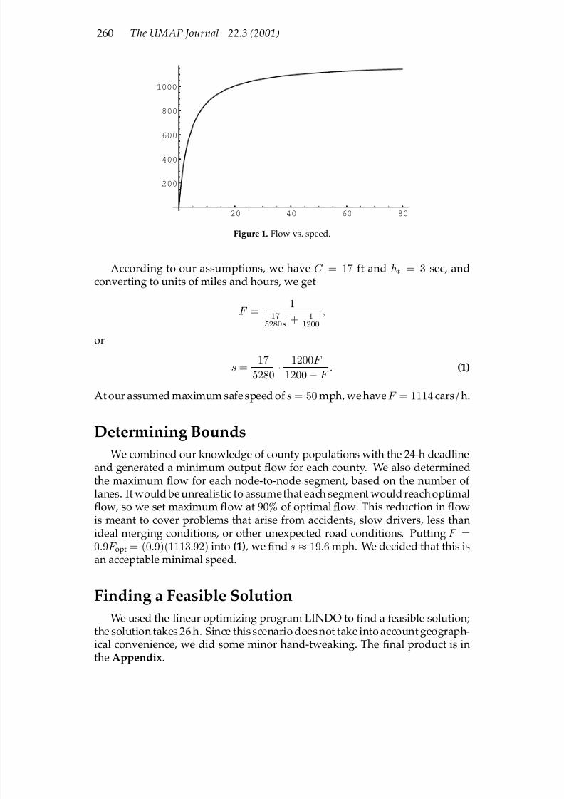
7/17/2019 UMAP 2001 vol. 22 No. 3



20 40 60 80

200

400

600

800

1000

Figure 1. Flow vs. speed.

According to our assumptions, we have C = 17 ft and ht = 3 sec, and

converting to units of miles and hours, we get

F = 117

5280s + 11200

,

or

s = 17

5280 · 1200F

1200− F . (1)

At our assumed maximum safe speed of s = 50 mph, we have F = 1114 cars/h.

Determining Bounds

We combined our knowledge of county populations with the 24-h deadlineand generated a minimum output ßow for each county. We also determinedthe maximum ßow for each node-to-node segment, based on the number of lanes. It would be unrealistic to assumethat each segment would reach optimalßow, so we set maximum ßow at 90% of optimal ßow. This reduction in ßowis meant to cover problems that arise from accidents, slow drivers, less thanideal merging conditions, or other unexpected road conditions. Putting F =0.9F opt = (0.9)(1113.92) into (1) , we Þnd s

≈19.6 mph. We decided that this is

an acceptable minimal speed.

Finding a Feasible Solution

We used the linear optimizing program LINDO to Þnd a feasible solution;the solution takes 26 h. Since this scenario does not take into account geograph-ical convenience, we did some minor hand-tweaking. The Þnal product is inthe Appendix.

7/17/2019 UMAP 2001 vol. 22 No. 3



The Simulation

To conÞrm the feasibility of our model, we conducted a computer simula-tion using Arena simulation software. The simulation encompassed 24 h of traf Þc ßow on the nine evacuation routes assuming 90% ßow ef Þciency. Themodel assumed that there was an unlimited number of vehicles ready to enterthe simulation in all counties. The time headway between entering vehicleswas considered to be normally distributed with a mean of 3 s and a standarddeviation of 1 s. The simulation veriÞed our model.

Implementation Requirements

For optimal performance of our model:

• Evacuees must follow the evacuation routes. The State of South Carolina

should notify speciÞ

c communities or households which route to take.• Flow must be monitored on all evacuation routes; this requires metering

entry of evacuees onto the evacuation routes. Allowing vehicles to enter anevacuation route too quickly may result in congestion at bottlenecks.

• Advance notiÞcation that there will be ticketing by photograph could en-force the restriction on towing boats and trailers, which might otherwise beignored.

Applying the ModelRequirement 1

If an evacuation order included both Charleston and Dorchester counties24 h prior to the predicted arrival of a hurricane, it would be necessary toreverse all four lanes of I-26 to ensure the evacuation of the entire population of the two counties. In our simulation runs, all of the exit routes from Charlestonand Dorchester ran at full capacity (all lanes reversed, 90% of maximum ßow)for 24 h to evacuate the counties completely. If the lanes are not reversed, it isdoubtful that the two counties could evacuate in a timely fashion.

Requirement 2

To optimize use of the available bandwidth while ensuring that the entirepopulation is displaced inland within 24 h, we opted for a simultaneous evac-uation strategy: All counties begin evacuation at the same time.

Since hurricanes typically arrive in South Carolina moving northward, astaggering strategy would evacuate southernmost counties Þrst. Our model

7/17/2019 UMAP 2001 vol. 22 No. 3



has discrete evacuation routes servicing each part of the coastline, so it is notnecessary to stagger evacuation. For example, since Beaufort County, whichwould be among the Þrst counties to be hit in the case of a hurricane, andHorry County, which would be hit signiÞcantly later, do not depend on thesame evacuation route, nothing is gained by delaying the evacuation of Horry

County until Beaufort County has cleared out.

Requirement 3

To evacuate the entire coastal region within 24 h, we found it necessaryto turn around traf Þc on all designated evacuation routes. With greater timeallowance, not all routes would need to be turned around.

Requirement 4

Ourmodel directs approximately 480,000 evacuees to Columbia. This surgeentering a city of 500,000 would undoubtedly disrupt traf Þc ßow. While threemajor interstates head farther inland from Columbia and could easily accom-modate the traf Þc from the coast, the extreme congestion within the city woulddisrupt the ßow coming into Columbia from the coast. It would be best to setup temporary shelters around the outskirts of Columbia (and at other destina-tion sites) to avoid having too many people vying for space within Columbiaitself.

Requirement 5

Because heavy vehicles take up more road space and generally require agreater headway time, they adversely affect our model. Heavy vehicles areallowable if they are the only available means of transportation, as may be thecase fortourists in recreational vehicles. Boats andtrailers arestrictly forbiddenontheevacuationroutes. Aruleofonecarperhouseholdcanbeannounced,butthe model can probably handle up to two cars per household. Our assumptionof two people per car can still hold up, given the number of people who areunable to drive themselves to safety.

Requirement 6With the ßow and time constraints deÞned within our model, the entrance

of large numbers of additional evacuees onto the designated evacuation routesfrom I-95 would cause serious disruptions. The traf Þc on I-95 coming fromGeorgia and Florida may turn west onto any nonevacuation roadway. Ideally, better evacuation routes could be established within Georgia and Florida tominimize their evacuees entering South Carolina.

7/17/2019 UMAP 2001 vol. 22 No. 3



Limitations

Time forced us to simplify our model. Here are extensions that we wouldhave liked to include:

Factor in the “Þrst-hour” effect. The western counties could potentially havefull use of the evacuation routes for a limited time at the very beginning of the evacuation. The population of the eastern counties would take time toreach the western counties; but once they did, both groups would have toshare the route.

Do more work with the impact of large vehicles.

Explore headway time in greater detail. We know that headway time is notdependent on speed in an ideal world, but does human psychology makeheadway time dependent on speed? Also, although we assume that allvehicles exhibit the same stopping pattern, we know that car size and brakecondition have an effect. We would like to Þnd a more accurate concept of headway time.

Inspect all nine routes on-site. We assume that any road listed by the SCDOTas a hurricane evacuation route is well maintained and appropriate for thatuse, and that these are the only appropriate routes.

Expand the complexity of our model. We kept the number of paths to a man-ageable level, but it would be nice to factor in the smaller routes.

Develop mechanisms to implement our model. Thiswould involve planning

out a block-by-block time-table, metering techniques, merging techniques,traf Þc reversal techniques, and large-vehicle restriction techniques.

Add accidents, breakdowns, and other problems to the model speciÞcally, ratherthan just lumping them into “ef Þciency.”

Study the potential costs of complete trafÞc reversal.

Study the population ßuctuations of Myrtle Beach, so that we would knowhow many tourists to expect in the event of a hurricane.

7/17/2019 UMAP 2001 vol. 22 No. 3



Authorities Fear Floyd Repeat,

Enlist Help of Undergraduates

Arden Hills, MN, Feb. 12—Responding to complaints over thedisorder of South Carolina’s 1999coastal evacuation in preparation forHurricane Floyd, authorities enlistedthe aid of three undergraduates fromBethel College. The task set beforethe three young mathematicians wasto plan an orderly and timely evacua-tion of South Carolina’s coastal region.

A denial of funding for travel ex-penses prevented the students frommaking an on-site inspection, but theymanaged to get a feel for the territory based on maps and census reports.Using a technique they dubbed “Ab-stracted Flow Modeling,” the teamconstructed several computer mod-els of what a full coastal evacuationwould involve. Using all the tools

availabletothemandalittlehumanin-tuition, the trio created a 26-hour sce-nario for the full evacuation of more

than 12 counties.Such an evacuation would involve

all people in the area being dividedamong 9 separate evacuation routesandreleased in a timed fashion. Usingthe timings and routings suggested bythe Bethel team, the entire coast could be evacuated within a reasonable timeand the travel time for individual ve-hicles could be kept to a minimum.

Compared to the 1999 evacua-tion, when fewer than 800,000 peoplewere evacuated, the Bethel model canevacuate more than 1.1 million peo-ple. Much of this increase can be at-tributed to grid-lock prevention, lane-doubling, and access restriction to themain highways.

Concerned citizens should be onthe lookout for announcements con-

cerning route assignments and depar-ture timings for their neighborhoods.

— Nathan Gossett, Barbara Hess, and Michael Page in Arden Hills, MN

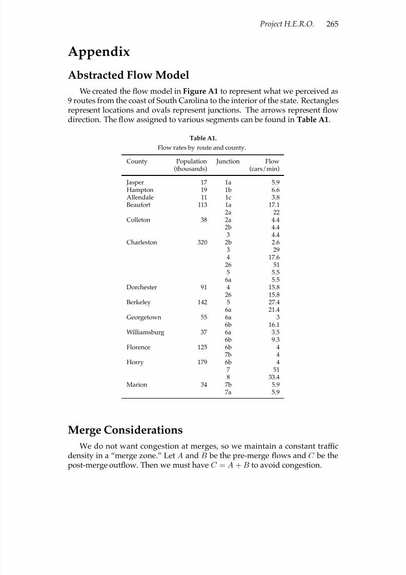
7/17/2019 UMAP 2001 vol. 22 No. 3



Appendix

Abstracted Flow Model

We created the ßow model in Figure A1 to represent what we perceived as

9 routes from the coast of South Carolina to the interior of the state. Rectanglesrepresent locations and ovals represent junctions. The arrows represent ßowdirection. The ßow assigned to various segments can be found in Table A1.

Table A1.

Flow rates by route and county.

County Population Junction Flow(thousands) (cars/min)

Jasper 17 1a 5.9Hampton 19 1b 6.6Allendale 11 1c 3.8Beaufort 113 1a 17.1

2a 22Colleton 38 2a 4.4

2b 4.43 4.4

Charleston 320 2b 2.63 294 17.6

26 515 5.5

6a 5.5Dorchester 91 4 15.8

26 15.8

Berkeley 142 5 27.46a 21.4

Georgetown 55 6a 36b 16.1

Williamsburg 37 6a 3.56b 9.3

Florence 125 6b 47b 4

Horry 179 6b 47 518 33.4

Marion 34 7b 5.97a 5.9

Merge Considerations

We do not want congestion at merges, so we maintain a constant traf Þcdensity in a “merge zone.” Let A and B be the pre-merge ßows and C be thepost-merge outßow. Then we must have C = A + B to avoid congestion.

7/17/2019 UMAP 2001 vol. 22 No. 3



Figure A1. Abstracted ßow model.

7/17/2019 UMAP 2001 vol. 22 No. 3



We must regulate the pre-merge ßows to prevent congestion and allow formaximum post-merge ßow.

If the density of merging traf Þc is large enough, we set aside one or twolanes for merging for about a mile prior to the merge point. We investigatewhether this is possible without lowering the pre-merge ßows A and B , and

when this strategy is physically possible and beneÞcial.Does shifting main-roadtraf Þc left to open a merge lane(s) increase the mainroad’s ßow (before merge traf Þc is added) and thus increase its contribution topost-merge ßow? If so, then the post-merge ßow would be

(A + increase) + B = (C + increase).

But weÞxed C = A +B as the maximum ßow, so A or B or both must decrease.Is this reduction really a concern?

Recall that F = ks , where F is ßow, k is density, and s is speed. Let N bethe number of cars on a one-mile stretch and L be the number of lanes in the

direction of concern. The total ß

ow of the road is the product of the lane ß

owand the number of lanes:

Lks = L(N/L)s = N s.

To shift one lane left, we must move N/L vehicles to L − 1 lanes, adding N/LL−1

vehicles to each non-merge lane, thus giving a new lane population of

N

L +

N/L

L− 1 =

N

L · L

L− 1.

So the new ßow is

(L− 1)

N L · L

L− 1

s = N s.

No change! We do not have to reduce pre-merge ßows to add a merge lane(assuming that the merge lane modiÞcation is physically possible). The sameargument conÞrms that pre-merging works for shifting two lanes.

When are these shifts physically possible? Let m = N/L , and let q be alane’s carrying capacity per mile, which is a function of s for Þxed ht. Then forclearing one merge lane to be physically possible, we need

m

L− 1 ≤q

−m.

If two lanes need to be shifted left, the same process yields the requirement

2m

L− 2 ≤ (q − m).

Moving everything to the right side of the inequalities gives two functions thatare greater than or equal to 0, each a function of L and m. We Þx L = 2 , 3 , and4 lanes and graph the functions to see when they are within the constraints.

7/17/2019 UMAP 2001 vol. 22 No. 3



Figure A2 shows valid and invalid ms given four lanes (two lines for twopossible shifts, single or double). We have q = 309.83 , the carrying capacity fora mile-long lane with s = 50 , and ht = 3 seconds. The function must lie on orabove the horizontal axis for creation of a merge lane.

50 100 150 200 250 300 350

-400

-300

-200

-100

100

200

Figure A2. Feasibility functions for one lane (thin line) and two lanes (thick line), as a function of the number of cars per mile (m = N/L).

The merge patrol of Þcer can determine q by multiplying the number of carscounted in one minute by 6/5. If the ratio of merging traf Þc to main-road traf Þcishigherthan 1 : 20 , theremay be enoughdisruptionthat mergeef Þciencycould beneÞt from a merge lane(s). With this ratio, and 90% ßow, there would be onecar merging every minute.

ReferencesGerlough, Daniel L., and Matthew J. Huber. 1975. Traf Þc Flow Theory. Trans-

portation Research Board.

Intergraph. www.intergraph.com/geoinfo/scdot.asp . Accessed 9 February2001.

Pressley, Sue Anne. 1999. As Hurricane Floyd approaches, record number of people moved. Washington Post 119, No. 42 (19 September 1999). Posted athttp://tech.mit.edu/V119/N42/floyd.42w.html . Accessed 9 February

2001.Rand McNally & Company. 1998. Skokie, IL: United States Road Atlas.

Scan21. 2001. http://www.scan21.com/hurricane_main.html . Accessed 9February 2001.

US Census. 2001. http://www.census.gov/population/estimates/county/co-99-1/99C1_45.txt. Accessed 9 February 2001.

7/17/2019 UMAP 2001 vol. 22 No. 3



US Department of Transportation. 2001. http://www.dot.state.sc.us . Ac-cessed 9 February 2001.

Winston, Wayne L. 1994. Operations Research. Duxbury Press.

7/17/2019 UMAP 2001 vol. 22 No. 3



7/17/2019 UMAP 2001 vol. 22 No. 3


Traf Þc Flow Models 271

TrafÞc Flow Models andthe Evacuation Problem

Samuel W. MaloneCarl A. MillerDaniel B. NeillDuke UniversityDurham, NC

Advisor: David P. Kraines

Introduction

We consider several models for traf Þc ßow. A steady-state model employsa model for car-following distance to derive the traf Þc-ßow rate in terms of empirically estimated driving parameters. We go on to derive a formula fortotal evacuation time as a function of the number of cars to be evacuated.

The steady-state model does not take into account variance in speeds of vehicles. To address this problem, we develop a cellular automata model fortraf Þc ßow in one and two lanes and augment its results through simulation.

After presenting the steady-state model and the cellular automata models,we derive a space-speed curve that synthesizes results from both.

We address restricting vehicle types by analyzing vehicle speed variance.

To assess traf Þ

c merging, we investigate how congestion occurs.We bring the collective theory of our assorted models to bear on Þve evac-uation strategies.

Assumptions

• Driver reaction time is approximately 1 sec.

• Drivers tend to maintain a safe distance; tailgating is unusual.

• All cars are approximately 10 ft long and 5 ft wide.

• Almost all cars on the road are headed to the same destination.


7/17/2019 UMAP 2001 vol. 22 No. 3



Terms

Density d: the number of cars per unit distance.

Occupancy n: the proportion of the road covered by cars.

Flow q : the number of cars per time unit that pass a given point.

Separation distance s: the average distance between midpoints of successivecars.

Speed v: the average steady-state speed of cars.

Travel Time: how long a given car spends on the road during evacuation.

Total Travel Time: the time until the last car reaches safety.

The Steady-State Model

Development

Car-following is described successfully by mathematical models; followingRothery [1992, 4-1], we model the average separation distance s as a functionof common speed v:

s = α + βv + γv2, (1)

where α, β, and γ have the physical interpretations:

α = the effective vehicle length L,

β = the reaction time, and

γ = the reciprocal of twice the maximum average deceleration

of a following vehicle.

This relationship allows us to obtain the optimal value of traf Þc density (andspeed) that maximizes ßow.

Theorem. For q = kV (the fundamental equation for traffic flow) and (1), traffic

flow q is maximized at

q ∗ = (β + 2γ 1/2L1/2)−1, v∗ = (L/γ )1/2, k∗ = β (γ/L)1/2 − 2γ

β 2 − 4γL .

Proof: Consider N identical vehicles, each of length L, traveling at a steady-state speed v with separation distance given by (1). If we take a freeze-framepicture of these vehicles spaced over a distance D , the relation D = N L + Ns

7/17/2019 UMAP 2001 vol. 22 No. 3



must hold, where s is the bumper-to-bumper separation. Since s = s−L , weobtain k = N/D = N/(NL + Ns) = 1/(L + s) = 1/s. We invoke (1) to get

k = 1

α + βv + γv2.

This is a quadratic equation in v; taking the positive root yields

v(k) = 1

2γ

4

γ

k + (β 2 − 4γL)− β

2γ .

Applying q = kv, we have

q (k) = k

2γ

4

γ

k + (β 2 − 4γL)− kβ

2γ .

Differentiating with respect to k, setting the result equal to zero, and wadingthrough algebra yields the optimal values given.

Interpretation and Uses

We can estimate q ∗, k∗, and v∗ from assumptions regarding car length (L),reactiontime (β ), andthedecelerationparameter(γ ). If welet L = 10 ft, β = 1 s,and γ ≈ .023 s2/ft (a typical value [Rothery 1992]), we obtain

q ∗ = 0.510 cars/s, v∗ = 20.85 ft/s, k∗ = 0.024 cars/ft.

A less conservative estimate for γ is γ = 12 (a−1f − a−1l ), where af and al are

theaverage maximum decelerations of thefollowingand lead vehicles Rothery[1992]. We assume that instead of being able to stop instantaneously (inÞnite

deceleration capacity), the leading car has deceleration capacity twice that of the following car. Thus, instead of γ = 1/2a = .023 s2/ft, we use the impliedvalue for a to compute γ = 1

2

a−1 − 2a−1

= 1

2 γ = 0.0115 s2/ft and get

q ∗ = 0.596 cars/s, v∗ = 29.5 ft/s ≈ 20 mph, k∗ = .020 cars/ft.

Going 20 mph in high-density traf Þc with a bumper-to-bumper separation of 40 ft is not bad.

The 1999 evacuation was far from optimal. Taking 18 h for the 120-mitrip from Charleston to Columbia implies an average speed of 7 mph and a bumper-to-bumper separation of 7 ft.

Limitations of the Steady-State Model

The steady-state model does not take into account the variance of cars’speeds. Dense traf Þc is especially susceptible to overcompensating or under-compensating for the movements of other drivers.

A second weakness is that the value for maximum ßow gives only a Þrst-order approximationof theminimumevacuationtime. Determiningmaximumßow is distinct from determining minimum evacuation time.

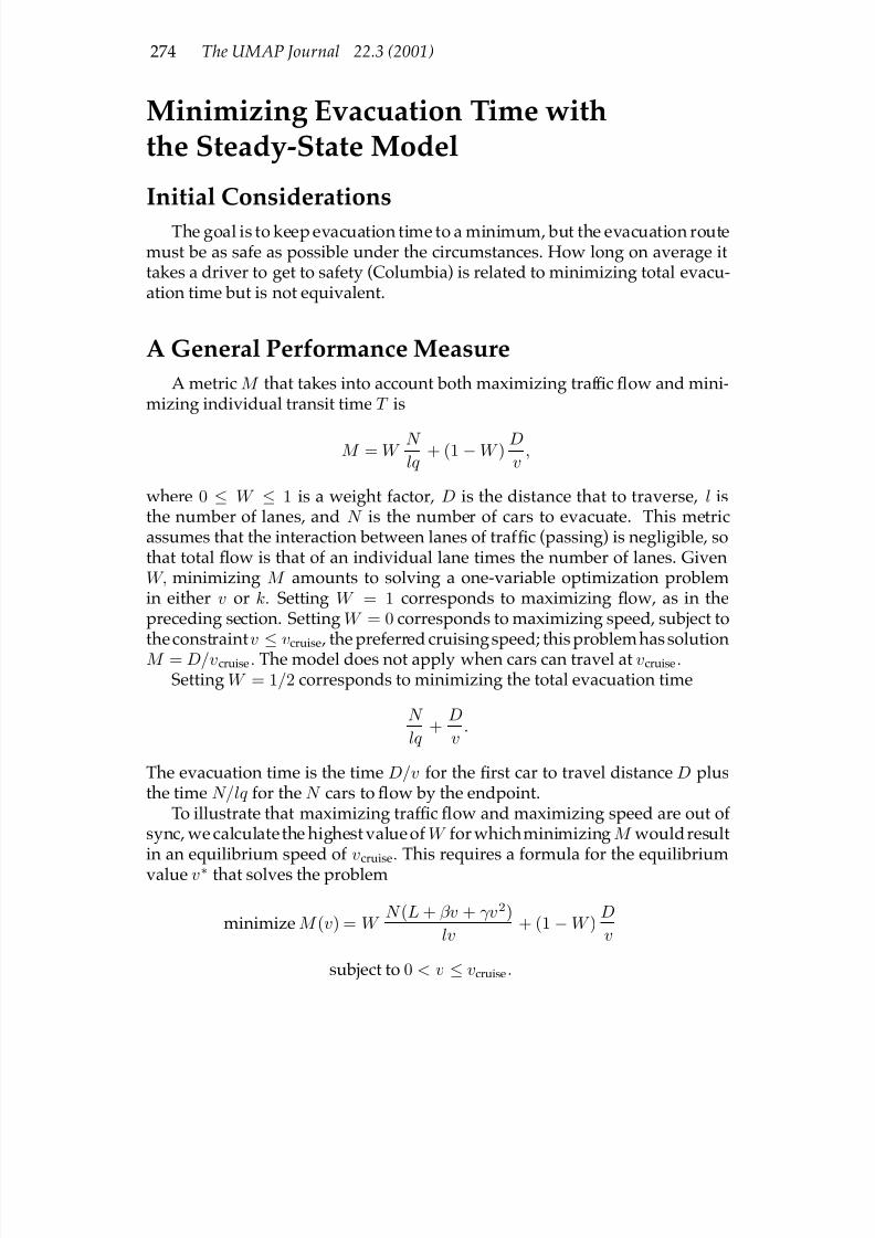
7/17/2019 UMAP 2001 vol. 22 No. 3



Minimizing Evacuation Time withthe Steady-State Model

Initial Considerations

The goal is to keep evacuation time to a minimum, but the evacuation routemust be as safe as possible under the circumstances. How long on average ittakes a driver to get to safety (Columbia) is related to minimizing total evacu-ation time but is not equivalent.

A General Performance Measure

A metric M that takes into account both maximizing traf Þc ßow and mini-mizing individual transit time T is

M = W N lq

+ (1−W ) D

v ,

where 0 ≤ W ≤ 1 is a weight factor, D is the distance that to traverse, l isthe number of lanes, and N is the number of cars to evacuate. This metricassumes that the interaction between lanes of traf Þc (passing) is negligible, sothat total ßow is that of an individual lane times the number of lanes. GivenW, minimizing M amounts to solving a one-variable optimization problemin either v or k. Setting W = 1 corresponds to maximizing ßow, as in thepreceding section. Setting W = 0 corresponds to maximizing speed, subject totheconstraintv

≤vcruise , the preferred cruisingspeed; this problemhas solution

M = D/vcruise. The model does not apply when cars can travel at vcruise.Setting W = 1/2 corresponds to minimizing the total evacuation time

N

lq +

D

v .

The evacuation time is the time D/v for the Þrst car to travel distance D plusthe time N/lq for the N cars to ßow by the endpoint.

To illustrate that maximizing traf Þc ßow and maximizing speed are out of sync, we calculate the highest value of W for whichminimizing M wouldresultin an equilibrium speed of vcruise. This requires a formula for the equilibriumvalue v∗ that solves the problem

minimize M (v) = W N (L + βv + γv2)

lv + (1−W )

D

v

subject to 0 < v ≤ vcruise.

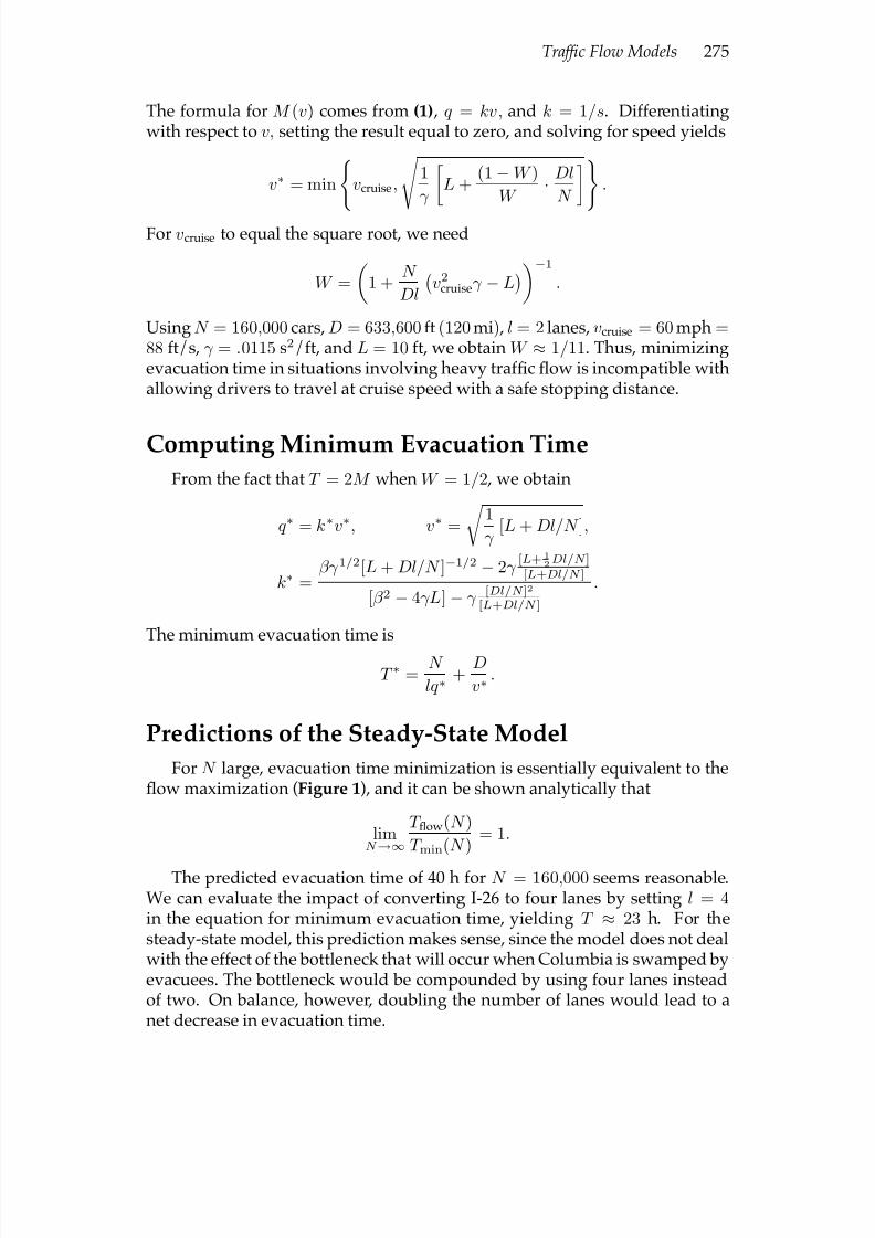
7/17/2019 UMAP 2001 vol. 22 No. 3



The formula for M (v) comes from (1) , q = kv, and k = 1/s. Differentiatingwith respect to v, setting the result equal to zero, and solving for speed yields

v∗ = min

vcruise,

1

γ

L +

(1− W )

W · Dl

N

.

For vcruise to equal the square root, we need

W =

1 +

N

Dl

v2cruiseγ − L

−1.

Using N = 160,000 cars, D = 633,600 ft (120 mi) , l = 2 lanes, vcruise = 60 mph =88 ft/s, γ = .0115 s2/ft, and L = 10 ft, we obtain W ≈ 1/11. Thus, minimizingevacuation time in situations involving heavy traf Þc ßow is incompatible withallowing drivers to travel at cruise speed with a safe stopping distance.

Computing Minimum Evacuation TimeFrom the fact that T = 2M when W = 1/2 , we obtain

q ∗ = k∗v∗, v∗ =

1

γ [L + Dl/N ],

k∗ =βγ 1/2[L + Dl/N ]−1/2 − 2γ

[L+ 1

2Dl/N ]

[L+Dl/N ]

[β 2 − 4γL]− γ [Dl/N ]2

[L+Dl/N ]

.

The minimum evacuation time is

T ∗ = N

lq ∗+

D

v∗.

Predictions of the Steady-State Model

For N large, evacuation time minimization is essentially equivalent to theßow maximization (Figure 1), and it can be shown analytically that

limN →∞

T ßow(N )

T min(N ) = 1.

The predicted evacuation time of 40 h for N = 160,000 seems reasonable.We can evaluate the impact of converting I-26 to four lanes by setting l = 4in the equation for minimum evacuation time, yielding T ≈ 23 h. For thesteady-state model, this prediction makes sense, since the model does not dealwith the effect of the bottleneck that will occur when Columbia is swamped byevacuees. The bottleneck would be compounded by using four lanes insteadof two. On balance, however, doubling the number of lanes would lead to anet decrease in evacuation time.

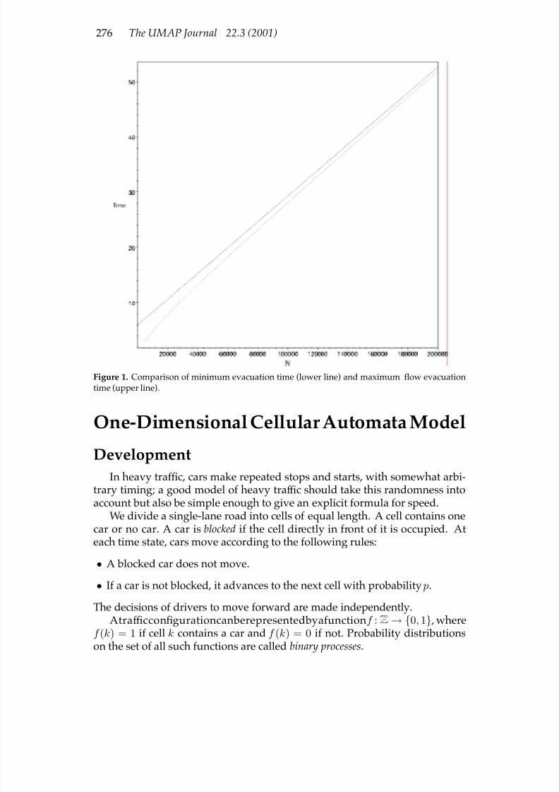
7/17/2019 UMAP 2001 vol. 22 No. 3



Figure 1. Comparison of minimum evacuation time (lower line) and maximum ßow evacuationtime (upper line).

One-Dimensional Cellular Automata Model

Development

In heavy traf Þc, cars make repeated stops and starts, with somewhat arbi-trary timing; a good model of heavy traf Þc should take this randomness intoaccount but also be simple enough to give an explicit formula for speed.

We divide a single-lane road into cells of equal length. A cell contains onecar or no car. A car is blocked if the cell directly in front of it is occupied. Ateach time state, cars move according to the following rules:

• A blocked car does not move.

• If a car is not blocked, it advances to the next cell with probability p.

The decisions of drivers to move forward are made independently.Atraf ÞcconÞgurationcanberepresentedbyafunctionf : Z → {0, 1} , where

f (k) = 1 if cell k contains a car and f (k) = 0 if not. Probability distributionson the set of all such functions are called binary processes.

7/17/2019 UMAP 2001 vol. 22 No. 3



Given a process X , deÞne a process I p(X ) according to the following rule:

If

X (i), X (i + 1)

= (1, 0)

then

I p(X )(i), I p(X )(i + 1)

=

(0, 1), with probability p;(1, 0), with probability 1

− p.

This rule is identical to the traf Þc ßow rule given above: If X represents thetraf Þc conÞguration at time t , I p(X ) gives the traf Þc conÞguration at time t + 1.

We are interested in what the traf Þc conÞguration looks like after severaliterations of I . Let I n p (X ) mean I p applied n times to X . The formula for traf Þcspeed in terms of density comes from the following theorem1:

Theorem. Suppose that X is a binary process of density d. Let

r = 1−

1− 4d(1− d) p

2 pd

and let M p,d denote the Markov chain with transition probabilities

0 −→

0, w/ prob. 1− r;

1, w/ prob. 1− r;1 −→

0, w/ prob. r ;

1, w/ prob. r.

The sequence of processes X, I p(X ), I 2 p(X ), I 3 p (X ), . . . converges to M p,d.

Here “density” means thefrequency with which 1s appear, analogous to theaveragenumberofcarspercell. Thistheoremtellswhatthetraf ÞcconÞgurationlooks like after a long period of time.

Knowingthetransition probabilitiesallowsustocompute easilytheaveragespeed of the cars in M p,d: the average speed is the likelihood that a randomlychosen car is not blocked and advances to the next cell at the next time state:

v = P r [I (M p,d(i)) = 0 |M p,d(i) = 1]

= P r [M p,d(i + 1) = 0 |M p,d(i) = 1]

· P r [I (M p,d(i)) = 0 |M p,d(i) = 1 andM p,d(i + 1) = 0]

= rp =

1−

1− 4d(1− d) p

2 pd

p =

1−

1− 4d(1− d) p

2d . (2)

Themodel does notaccurately simulate high-speed traf Þcanddoesnottakeinto account following distance, andthe stop-and-start model of car movementis not accurate when traf Þc is sparse. The model is best for slow traf Þc (under15 mph) with frequent stops.

1This theorem is the result of previous research [Miller 2001] by an author of this paper. TheAppendix on binaryprocesses (written duringthe contest period) gives a relatively complete proof of the result. [EDITOR’S NOTE: We unfortunately must omit the Appendix.]

7/17/2019 UMAP 2001 vol. 22 No. 3



Low Speeds

We must set three parameters:

∆x = the size of one cell, the space taken up by a car in a tight traf Þc jam; weset it to 15 ft, slightly longer than most cars.

∆t = the length of one time interval, the shortest time by a driver to move intothe space in front; we take this to be 0.5 s.

p = themovementprobability, representingtheproportionof driverswhomoveat close to the overall traf Þc speed; we let p = 0.85.

In (2) we insert the factor (∆x/∆t) to convert from cells/time-state to ft/s:

v =

∆x

∆t

1−

1− 4d(1− d) p

2d .

Density d is incars per cell, related to occupancy n by d = (15 ft/10 ft)×n = 3n/2.Table 1 gives v for various values of n and k.

Table 1.

v for various values of n and k.

n K d vft−1 (mph)

0.60 0.060 0.90 20.55 0.055 0.83 40.50 0.050 0.75 50.45 0.045 0.68 80.40 0.040 0.60 100.35 0.035 0.53 120.30 0.030 0.45 140.25 0.025 0.38 150.20 0.020 0.30 16

One Lane

To explore theone-dimensionalcellular automata model, we wrotea simplesimulation in C++. The simulation consists of a 5,000-element long (circular)array of bits, witha 1 representinga car and a 0 representinga (car-sized) emptyspace. The array is initialized randomly based on a value for the occupancy n:An element is initialized to 1 with probability n , or to 0 with probability 1− n.The array is iterated over 5,000 time cycles: On each cycle, a car moves forwardwith probability p if the square in front of it is empty. The ßow q is calculatedas the number of cars N passing the end of the array divided by the number of time cycles (i.e., q = N/5000), and thus the average speed of an individual carin cells per time cycle is v = q/n = N/5000n.

7/17/2019 UMAP 2001 vol. 22 No. 3



Table 2.

Comparison of simulation and equation values for speed.

Speed

p = 1/2 p = 3/4n Simulation Equation Simulation Equation

0.2 0.433 0.438 0.694 0.6970.4 0.356 0.349 0.592 0.5890.6 0.234 0.232 0.392 0.3920.8 0.108 0.110 0.171 0.174

Table 2 shows results for various values of the occupancy n and probability p , verifying the accuracy of the one-dimensional cellular automata equation (2).

The value for p should be related to the mean and standard deviation of vcruise. The mean and standard deviation of a binary random variable are p and

p(1−

p). We have

p p(1− p)

= µ

σ −→ p =

1

1 +σµ

2 .

For µ(vcruise) = 60 mph and σ(vcruise) = 5 mph, we get p = 144/145. Now,L = µtp; so assuming L = 10 ft, p = 144/145 , and µ = 60 mph = 88 ft/s, weobtain a time step of 0.113 s.

We now use the model to predict how fast (on average) a car moves in asingle lane, as a functionof theoccupancy. We consider the“relative speed”vrel ,the average speed divided by the (mean) cruise speed. The average speed is

given by the one-dimensional cellular automata equation, and the cruise speedis p cells per time cycle, so this gives us

vrel = vavg

vcruise=

1−

1− 4n(1− n) p

2 pn .

Using p = 144/145 , we calculate vrel and vavg as a function of n (Table 3).The model predicts that for low occupancy the average speed will be near

the cruise speed, but for occupancies greater than 0.5 the average speed will be signiÞcantly lower. The cellular automata model does not take followingdistance into account; thus, it tends to overestimate vavg for high speeds and ismost accurate when occupancy is high and speed is low.

Table 3 also shows ßow rate q = nvavg/L , in cars/s, as a function of occu-pancy. The ßow rate is symmetric about n = 0.5. Each car movement can bethought of as switching a car with an empty space, so the movement of cars tothe right is equivalent to the movement of holes to the left.

The model fails, however, to give a reasonable value for the maximum ßowrate: 4.1 cars/s≈ 14,600 cars/h, about seven times a reasonable maximum rate[Rothery 1992]. The reason is that the cell size equals the car length, a correct

7/17/2019 UMAP 2001 vol. 22 No. 3



Table 3.

Relative speed, average speed, and ßow rate as a function of occupancy.

n vrel vavg ßow rate(ft/s) (ft/s) (cars/s)

0.1 .999 88 0.9

0.2 .998 88 1.80.3 .995 88 2.60.4 .987 87 3.50.5 .923 81 4.10.6 .658 58 3.50.7 .426 38 2.60.8 .249 22 1.80.9 .111 10 0.9

approximation only as car speeds approach zero and occupancy approaches 1.For n

≥0.5 , we should have a larger cell size; so we assume that cell size equals

car length plus following distance and that following distance is proportionalto speed. Assuming a 1 s following distance, we obtain cell size as

C = L + vavg × (1 sec).

But we do not know the value of vavg until we use the cell size to obtain it! Forn large, we can assume that vavg ≈ vcruise and Þnd an upper bound on cell size:

C = L + vcruise × (1 sec) = 98 ft.

We divide the original ßow rate by the increased cell size to obtain a morereasonable ßow rate:

q = 4.063 cars/s

98 ft/10 ft = 0.415 cars/s ≈ 1,500 cars/h.

This is likely to be an underestimate; for greater accuracy, we must Þnd amethod to compute the correct cell size before Þnding the speed. We addressthis problem later.

Two Lanes

We expand the one-dimensional model. The simulation consists of a two-dimensional (1000 × 2) array of bits. The array is initialized randomly andthen iterated over 1,000 time cycles: On each cycle, a car moves forward withprobability p if the cell in front of it is empty. If not, provided the cells besideit and diagonally forward from it are unoccupied, with probability p the carchanges lanes and moves one cell forward.

Like the one-lane simulation, the two-lane one is correct only for high den-sities and low speeds, since it uses cell size equal to car length. Hence, we donot use the two-lane simulation to compute the maximum ßow rate. However,

7/17/2019 UMAP 2001 vol. 22 No. 3



since cell size affects ßow rate by a constant factor, we can compare ßow rates by varying parameters of the simulation. In particular, we use this model toexamine how the ßow rate changes with the variance of speeds.

“But I Want to Bring My Boat!”There are two main types of variance in speeds:

• σ2t of traveling speed (random ßuctuations in the speed of a single vehicle

over time), and

• σ2m of mean speed (variation in the mean speeds of all vehicles).

In the one-lane simulation, we assumed that σm = 0 and σt = 5 mph; thischoice was reßected in the calculation of p , since p = 1/[1 + (σt/µ)2] for everycar. When we take σm into account, each car gets a different value of p:

• Choose the car’s mean speedµ

randomly from the normal distribution withmean vcruise and standard deviation σm.

• The car’s traveling speed will be normally distributed with mean µ andstandard deviation σt.

• The car’s transition probability p is

p = µ

vcruise + λσm

1

1 +σtµ

2 ,

where λ is a constant best determined empirically. We use λ = 0 , a conser-vative estimate of the change in ßow rate as a function of σm.

We consider what effect σt and σm have on the speed at a given occupancy.Considering the cars’ movement as a directed random walk, increasing σt in-creases randomness in the system, causing cars to interact (and hence block one other’s movement) more often, decreasing average speed.

The effects of σm are even more dramatic: Cars with low mean speedsimpede faster cars behind them.

We ran simulations in which we Þxed n = 0.5 and varied both σm and σt

from 0 to 15 mph. For each pair of values, we calculated average ßow rate forthe one- and two-lane simulations.

Table 4 shows the effects of lane-changing by comparing maximum ßowsfor the two-lane model with twice that for the one-lane model. For small σt andσm , allowing cars to switch lanes does not increase the ßow rate much; for highvalues, the two-lane model has a much higherßow rate. Each 5 mph increase inσm results in an 11–16% decrease in ßow rate (two-lane model, σt = 0), whileeach 5 mph increase in σt results in a 5–7% decrease in ßow rate (two-lanemodel, σm = 0). Both variances dramatically affect ßow rate, and σm is moresigniÞcant than σt.

7/17/2019 UMAP 2001 vol. 22 No. 3



Table 4.

Two-lane average ßow / Twice the one-lane average ßow.

σtσm 0 5 10 15

0 979/976 923/908 856/830 805/776

5 822/757 817/746 790/729 753/68310 699/537 691/518 659/485 642/46915 588/393 569/366 540/319 518/292

”So, Can I Bring My Boat?”

We considerhowvariations in vehicle type affect σm , σt , andßow rate. Mostlarge vehicles (boats, campers, semis, and motor homes) travel more slowlythan most cars. A signiÞcant proportion of large vehicles results in increasedσm and hence a lower ßow rate.

As a simpliÞ

ed approximation, we assume that there are two types of ve-hicles: fast cars (µ = µ1) and slow trucks (µ = µ2), with proportion α of slowtrucks α. We calculate

σ2m = α(µ2 − µ)2 + (1− α)(µ1 − µ)2

= α

µ2 −

µ1 − (µ1 − µ2)α2

+ (1− α)

µ1 − (µ1 − µ2)α2

= (µ1 − µ2)2

α2(1− α) + α(1− α)2

= (µ1 − µ2)2α(1− α).

Thus, σm = (µ1 − µ2)

α(1− α). We now assume that fast cars travel atµ1 = 70 mph and slow trucks at µ2 = 50 mph and Þnd σm as a function of α. Random ßuctuations in vehicle speed are likely to depend more on driverpsychology than on vehicle type, so we assume σt = 5 mph. We interpolatelinearly in Table 4 toÞnd the ßow rate (cars per 1,000 time cycles) as a functionof the proportion of slow vehicles α (Table 5).

Table 5.

Flow rate as a function of proportion of slow vehicles.

α σt ßow rate % reduction in ßow

0 0 923/908 0/0.01 1.99 881/844 4.6/7.0.02 2.80 864/817 6.4/10.0

.05 4.36 831/767 10.0/15.5.1 6.00 792/700 14.1/22.9.2 8.00 741/609 19.7/32.9.5 10.0 691/518 25.1/43.0

The ßow rate is decreased signiÞcantly by slow vehicles: If 1% of vehiclesare slow, theßow rate decreases by 5%; if 10% of vehicles are slow, the ßow ratedecreases by 15%. The effects of σm are magniÞed if vehicles are unable to passslower vehicles; so if the highway went down to one lane at any point (due to

7/17/2019 UMAP 2001 vol. 22 No. 3



construction or accidents, for example), the ßow rate would be reduced evenfurther. Hence, we recommend no large vehicles (vehicles that may potentially block multiple lanes) and no slow vehicles (vehicles with a signiÞcantly lowermean cruising speed). Exceptions couldbe made if a familyhasno othervehicleand for vehicles with a large number of people (e.g., buses). Slow-moving

vehicles should be required to stay in the right lane and families should beencouraged to take as few vehicles as possible.

The Space-Speed Curve

Todetermineoptimaltraf Þcßowrates,wecancombine theone-dimensionalcellular automata and the steady-state models to get a good estimate of therelationship between speed v and the separation distance s.

s ≤ 15: There is essentially no traf Þc ßow: v(s) = 0.

15 ≤ s ≤ 30: Traf Þc travels at between 0 and 12 mph and the one-dimensionalcellular automata model applies; v is approximately a linear function of s.

30 ≤ s ≤ 140: Traf Þc travels between 12 and 55 mph and the steady-statemodel is appropriate; v is again approximately a linear function of s , withless steep slope.

140 ≤ s: Traf Þc travels at the speed limit of 60 mph.

Incoming TrafÞc Rates

The optimal ßow is determined by the optimal ßow through the smallest bottleneck. However, the time of travel (which is a more important measurefor our purposes) is affected by other factors, including the rate of incomingtraf Þc. If incoming traf Þc is heavy, congestion occurs at the beginning of theroute, decreasing speed and increasing travel time for each car.

How does congestion occur and how much does it inßuence travel time?Consider the one-dimensional cellular automata model with p = 1/2. Repre-sent the road by the real line and let F (x, t) denote the density of cars at point xon the road at time t. (For our purposes now, the cells and cars are inÞnitesimalin length.) Suppose that the initial conÞguration F (x, 0) is given by

F (x, 0) =

1, if x < 0;0, if x ≥ 0.

This represents a dense line of cars about to move onto an uncongested road.We omit units for the time being. By formulas derived earlier, the speed

v(x0, t0) at position x0 and time t0 is given by

v(x0, t0) = 1−

1− 2F (x0, t0)[1− F (x0, t0)]

2F (x0, t0) ,

7/17/2019 UMAP 2001 vol. 22 No. 3



while speed must also equal the rate at which the number of cars past point xis increasing; that is,

v(x0, t0) = d

dt

∞

x

F (x, t)dx

(t0) .

Thus,

dF

dt = −dv

dx = − d

dx

1−

1− 2F (1− F )

2F

.

This is a partial differential equation whose unique solution is

F (x, t) =

1, if x/t < −12 ;

12 − (x/t)√

2−4(x/t)2, if − 1

2 ≤ x/t ≤ 12 ;

0, if 12 < x/t.

Thus, after a steady inßux of cars for a period of ∆t , the resulting congestion is1

2 −

x∆t

2− 4 x∆t

2and the congestion ends at x = ∆t/2.

Thus, the extent of the congested traf Þc is linear in ∆t. So if there is a steadyinßux of cars onto a highway, the extent of the resulting congestion is directlyproportional to how long it takes them to enter, thus to the number N of them.Likewise, the time for the congestion to dissipate is proportional to N .

This allowsustoevaluatestaggering evacuation timesfordifferentcounties.

Suppose thatn countieshavepopulations P 1, . . . , P n. If all evacuateat the sametime, the effect of the resulting traf Þc jam on total travel time is proportional tothe product of the extent of the jam and the time before it dissipates:

∆T travel time = c1 · c2 (P 1 + · · ·+ P n) · c3 (P 1 + · · ·+ P n)

= c1c2c3 (P 1 + · · ·+ P n)2

for some constants c1, c2, c3. If the evacuations are staggered, the effect is

∆T travel time = c1c2c3P 21 + · · ·+ c1c2c3P 2n = c1c2c3

P 21 + · · ·+ P 2n

.

Now, P 21

+· · ·

+ P 2n

< (P 1 +· · ·

+ P n)2; so unless one of the counties has amuch larger population than the rest, the difference between these two valuesis relatively large. We therefore recommend staggering counties.

The Effects of Merges and Diverges

While thesteady-statemodel is a reasonably accurate predictor of traf Þc behav-ior on long homogeneous stretches of highway, we must also consider how to

7/17/2019 UMAP 2001 vol. 22 No. 3



deal with the effects of road inhomogeneities: merges of two lanes into a singlelane and “diverges” of one lane into two lanes. To do so, we apply the princi-ple of conservation of traf Þc [Kuhne and Michalopolous 1992]. Assuming thatthere are no sources or sinks in a region, we have

∂q ∂x + ∂k∂t = 0,

where q is ßow rate (cars/s), k is density (cars/ft), x is location (ft), and t istime (s). Let the merge or diverge occurs at a speciÞc point x. In the steadystate (i.e., for ∂D/∂t = 0), we have ∂q/∂x = 0 , so ßow conserved at a junction.

For a ßow q s merging or divergingßows q 1 and q 2 , we have q s = q 1 + q 2. If proportion P (0 < P < 1) of the ßow q s going to (or coming from) q 1 , and weknow either density (ks or k1), we can solve for the other density:

q 1 = P q s, k1v1 = P ksvs, k1v(k1) = P ksv(ks).

From the steady-state model, for the given values of the constants, we know

v(k) =

88 ft/s , 0 < k < 0.0056;

21.7

.08 + .092k − 1

, 0.0056 < k < 0.1.

Assuming that both densities are greater than the free-travel density k = .0056 ,we can set

k1

.08 +

.092

k1− 1

= P ks

.08 +

.092

ks− 1

.

Given either ks or k1 , we can solve numerically for the other. Then we can Þndthe speeds associated with each density using the above expression for v(k).

Solving the equation gives two values; we assume that the density is greateron the single-lane side of the junction (i.e., density increases at a merge anddecreases at a diverge). Also, if solving produces a speed v1 that is larger thanvcruise , we set v1 = vcruise and calculate n1 = q 1/v1.

How is the steady-state ßow rate determined on a path with merges anddiverges? Following Daganzo [1997], we consider a bottleneck to be a location(such as a merge or diverge) where queues can form and persist with free ßowdownstream. The bottleneck capacity is the maximum ßow rate through the

bottleneck, which (with Daganzo) we assume to be constant. If a steady-stateßow greater than the bottleneck capacity attempts to enter the bottleneck, thequeue size will increase until it stretches all the way back to its origin. At thatpoint, the steady-stateßow is blocked by the queue of cars and decreases to the bottleneck capacity. Hence, the maximum steady-state ßow rate along a pathis the minimum capacity of all bottlenecks along the path.

7/17/2019 UMAP 2001 vol. 22 No. 3



Parallel Paths

From A to B , let there be multiple parallel paths p1, . . . , pm with bottleneck capacities c1, . . . , cm. The maximum steady-state ßow rate from A to B is theminimum of:

• the bottleneck capacity of the diverge at point A ,

• the bottleneck capacity of the merge at point B , and

• the sum of the bottleneck capacities of all paths pi.

If a path has no bottlenecks, its capacity is the maximum ßow rate predicted by the steady-state model.

We focus on maximizing ßow rate rather than minimizing evacuation time,since for a large number of cars, maximizing ßow gives near-minimal evacua-tion time. The maximum ßow rate q max from Charleston to Columbia is

q max = min

i

q i, c0, cf

,

where q i is the maximum ßow rate of path i , c0 is the bottleneck capacity of Charleston, and cf is the bottleneck capacity of Columbia. Theßow rates q i are

q i = min(b1 . . . bn, q i,ss),

where b1, . . . , bn are the capacities of bottlenecks along the given route and q i,ssis the maximum ßow along that route as predicted by the steady-state model.

We Þ

rst consider evacuation with no bottlenecks along I-26. Denoting thesteady-statevalue q I-26,ss by q I , thisgives us q max = min(q I , c0, cf ). Whichfactorlimits q max? We cannot achieve q I ≈ 2,000 cars/h if if either c0 < 2,000 (traf Þc jam in Charleston) or cf < 2,000 (traf Þc jam in Columbia). With the traf Þc inColumbia splitting into three different roads, there should be less congestionthere than with everyone merging onto I-26 in Charleston. Hence, we assumethat c0 < cf , so the limiting factor is c0 if c0 < 2,000 and q I if c0 > 2,000.The value of c0 is best determined empirically, perhaps by extrapolation fromCharleston rush-hour traf Þc data or from data from the 1999 evacuation.

Effects of Proposed StrategiesReversing I-26

Reversing I-26 doubles q I to 4,000 cars/h. It is likely to increase c0 as well,since cars can be directedto two different paths onto I-26 and are thus less likelyto interfere with the merging of cars going on the other set of lanes. On the otherhand, twice as many cars will enter the Columbia area simultaneously, and the

7/17/2019 UMAP 2001 vol. 22 No. 3



unchanged capacity cf may become the limiting factor. It may be possible toincrease cf by rerouting some of the extra traf Þc to avoid Columbia, or eventurning around traf Þc on some highways leading out of Columbia.

Thus, this strategy is likely to improve evacuation traf Þc ßow.

Reversing Other HighwaysA similar argument applies to turning around the traf Þc on the smaller

highways. Each highway adds some capacity to the total

i q i , increasing thisterm, but each highway’s capacity is signiÞcantly less than q I , and increas-ing the number of usable highways has unclear effects on c0. It may increasecapacity by spreading out Charleston residents to different roads, or crossingevacuation routes may lead to traf Þc jams. As with the reversal of I-26, rever-sal of smaller highways does not affect cf (unless crossing evacuation routes becomes a problem in Columbia). More important, the interactions betweenhighways (merges and diverges) may lead to bottlenecks, reducing capacity.

In fact, interactions between these highways and I-26 could cause bottlenecksthat slow the ßow on I-26, perhaps offsetting the extra capacity of the smallerhighways. Thus, it is safer not to turn aroundtraf Þc on thesecondary highwaysor to encourage using these as evacuation routes.

Temporary SheltersEstablishing temporary shelters in Columbia, to reduce the traf Þc leaving

that city, couldbe useful ifonly some of thecars are directedinto Columbia; thusthe ßow of traf Þc in the Columbia area would be split into four streams ratherthan three, possibly increasing cf . Nevertheless, we hesitate to recommend this

strategy, since the actual effects are likely to be the opposite. Evacuees enteringColumbia are likely to create congestion there, making it dif Þcult for traf Þc toenter, resulting in a major bottleneck. Without careful regulation, more peoplewill try to stay in Columbia than the available housing, and frantic attempts of individuals driving around looking for housing will exacerbate the bottleneck.Hence, it is most likely that cf will decrease signiÞcantly, probably becomingthe limiting factor on maximum ßow rate.

Staggering TrafÞc FlowsStaggering is likely to reduce the time for an average car to travel from

Charleston to Columbia while leaving the value of the steady-state ßow rateq I unchanged. Hence, staggering decreases total evacuation time; it may alsoincrease maximum ßow rate, since it decreases the number of cars travelingtoward I-26 at any one time, reducing the size of the co bottleneck. Increasingthe capacity co , however, increases the ßow rate only when co is the limitingfactor.

7/17/2019 UMAP 2001 vol. 22 No. 3



Evacuees from Florida and GeorgiaSince evacuation time is proportional to number of cars over ßow rate, out-

of-state evacuees add to total evacuation time unless they take a route that doesnot intersect the paths of the South Carolina evacuees. However, it is very hardto constrain the routes of out-of-state evacuees, since they come from a variety

of paths andare unlikelyto be informed of thestate’s evacuation procedures. Inparticular, major bottlenecks are likely at the intersections of I-26 with I-95 andof I-95 with I-20 and U.S. 501. If many cars from I-95 attempt to go northweston I-26 toward Columbia, q I will no longer equal 2,000 cars/h but instead thecapacity of the I-26/I-95 bottleneck. This is likely to reduce q I signiÞcantly andlikely make q I −26 the limiting factor.

A similar argument suggests that I-95 traf Þc will impede the ßow of traf Þcwest from MyrtleBeach by causing a bottleneck at theI-95/I-20 junction. Traf Þcßow from Myrtle Beachis less than from Charleston, and many of the cars fromI-95 may have already exited at I-26; so the bottleneck at the I-20 junction islikely to be less severe. Nevertheless, the ßow of evacuees from Florida andGeorgia has the potential to reduce dramatically the success of the evacuation.

References

Daganzo, C.F., et al. 1997. Causes and effects of phase transitions in highwaytraf Þc. ITS Research Report UCB-ITS-RR-97-8 (December 1997).

Gartner, Nathan, Carroll J. Messer, and Ajay K. Rathi. 1992. Traf Þc Flow Theory:A State of the Art Report. Revised monograph. Special Report 165. Oak Ridge, TN: Oak Ridge National Laboratory. http://www.tfhrc.gov/its/tft/tft.htm .

Kuhne, R., and P. Michalopolous. 1992. Continuumßow models. Chapter 5 inGartner et al. [1992].

Miller, Carl A. 2001. Traf Þc ßow, random growth models, and the longestcommon subsequence problem. In preparation.

Rothery, R.W. 1992. Car following models. Chapter 4 in Gartner et al. [1992].

7/17/2019 UMAP 2001 vol. 22 No. 3



Modeling Hurricane

Evacuation Strategies

Durham, NC, Feb. 12— Hur-ricanes pose a serious threat to citi-zens on the South Carolina coastline,as well as other beach dwellers inFlorida, Georgia, and other neighbor-ing states. In 1999, the evacuation ef-fort preceding the expected landfall of Hurricane Floyd led to a monumen-tal traf Þc jam that posed other, alsoserious, problems to the more than

500,000 commuterswhoßedthecoast-line and headed for the safe havenof Columbia. Several strategies have been proposed to avoid a futurerepeatof this traf Þc disaster.

First, it has been suggested thatthe two coastal bound lanes of I-26 be turned into two lanes of Columbia bound traf Þc. A second strategywould involve staggering the evacua-tion of the coastal counties over some

time period consistent with how hur-ricanes affect the coast, instead of allat once. Third, the state might turnaround traf Þc ßow on several of thesmaller highways besides I-26 that ex-tend inland from the coast. The fourthstrategy under consideration is a planto establish more temporary sheltersin Columbia. Finally, the state isconsidering placing restrictions on the

type and number of vehicles that can be brought to the coast.In the interest of the public, we

have developed and tested severalmathematical models of traf Þc ßowto determine the ef Þcacy of each pro-posal. On balance, they suggest thatthe Þrst strategy is sound and should

be implemented. Although doublingthe number of lanes will not necessar-ily cut the evacuation time in half, oreven double theßowrateonI-26awayfrom the coast, it will signiÞcantly im-prove the evacuation time under al-most any weather conditions.

Our models suggest that stagger-ing the evacuation of different coun-ties is also a good idea. Taking such

action on the one hand will reducethe severity of the bottleneck thatoccurs when the masse of evacueesreaches Columbia, and on the otherhand could potentially increase aver-age traf Þc speed without signiÞcantlyincreasing traf Þc density. The net ef-fect of implementing this strategy willlikely be an overall decrease in coastalevacuation time.

The next strategy, which sug-

gests turning traf Þc around on sev-eral smaller highways, is not so easyto recommend. The main reason forthis is that the unorganized evacua-tion attempts of many people on fre-quently intersecting secondary roadsis a recipe for inef Þciency. In placeswhere these roads intersect I-26, themerging of a heightened volume of secondary road traf Þc is sure to cause

bottleneckson the interstate that couldsigniÞcantly impede ßow. To make astrategy of turning around traf Þc onsecondary roads workable, the statewould have to use only roads thathave a high capacity, at least twolanes,and a low potential for traf Þc conßictswith other highways. This would re-

7/17/2019 UMAP 2001 vol. 22 No. 3



quire competent traf Þc managementdirected at avoiding bottlenecks andmovingCharlestontraf ÞctoColumbiawith as few evacuation route conßictsas possible.

The fourth proposal, of estab-lishing more temporary shelters inColumbia, is a poor idea. Becauseit is assumed that travelers are rela-tively safe once they reach Columbia,themainobjectiveoftheevacuationef-fort should be minimizing the transittimetoColumbiaandthesurroundingarea. It is fairly clear that increasingthe number of temporary shelters inColumbia would lead to an increased

volume of traf Þc to the city (by rais-ing expectations that there will be free beds there) and exacerbate the traf Þcproblem in the city itself (due to anincreased demand for parking). To-gether, these two factors are sure toworsen the bottleneck caused by I-26traf Þc entering Columbia and wouldprobably increase the total evacuationtime by decreasing the traf Þc ßow on

the interstate.The Þnal proposal of placing lim-itations on the number and types of vehicles that can be brought to the beach is reasonable. Families withseveral cars should be discouragedfrom bringing all of their vehicles andperhaps required to register with thestate if the latter is their intention.Large, cumbersome vehicles such asmotor homes should be discouraged

unless they are a family’s only op-

tion. Although buses slow down traf-Þc, theyare beneÞcial because they ap-preciably decrease the overall numberof drivers. In all cases, slow-movingvehiclesshouldberequiredto travel in

the right lane during the evacuation.In addition to the strategies men-tioned above, commuters in the 1999evacuation were acutely aware of the effect on traf Þc ßow produced by coastal residents of Georgia andFlorida traveling up I-95. We haveconcluded that, when high-volumetraf Þc ßows such as these compete forthe same traf Þc pipeline, the nearlyinevitable result is a bottleneck. A

reasonable solution to this problemwould be to bar I-95 traf Þc from merg-ing onto I-26 and instead encourageand assist drivers on I-95 to use themore prominent, inland bound sec-ondary roads connected to that inter-state.

To conclude, we think that com- bining the more successful strategiessuggested could lead to a substantial

reduction in evacuation time, the pri-mary measure of evacuation success.Minimizing the number of accidentsthat occur en route is also important, but our models directed at the formergoal do not make compromises withthe latter objective. In fact, the prob-lem of minimizing accidents is chießytaken care of by ensuring that traf Þcßow is as orderly and ef Þcient as pos-sible.

— Samuel W. Malone, Carl A. Miller, and Daniel B. Neill in Durham, NC

7/17/2019 UMAP 2001 vol. 22 No. 3


The Crowd Before the Storm 291

The Crowd Before the Storm

Jonathan David CharlesworthFinale Pankaj Doshi

Joseph Edgar GonzalezThe Governor’s Schoolrenamed August 2001:Maggie L. Walker Governor’s School

for Government and International StudiesRichmond, VA

Advisor: John A. Barnes

IntroductionApplying safety regulations and ßow-density equations, we Þnd the maxi-

mum rate of ßow through a lane of road is 1,500 cars/h, occurring when carstravel at 27.6 mph.

We construct a computer simulation that tracks the exit of cars throughSouth Carolina’s evacuation network. We attempt to optimize the network byreversing opposing lanes on various roads and altering the time that each cityshould begin evacuating, using a modiÞed genetic algorithm.

Thebest solution—theonethat evacuates themost people in 24 h—involvesreversing all the opposing lanes on evacuation routes. Increasing the holding

capacity of Columbia is only marginally helpful. Georgia and Florida traf Þcon I-95 is only mildly detrimental, but allowing people to take their boats andcampers greatly decreases the number of people that can be evacuated.

Background on Evacuation Plans

After the1999evacuation, theSouth Carolina Departmentof Transportation(SCDOT) designated evacuation routes for all major coastal areas, including 14different ways to leave the coast from 32 regions. The routes take evacuees pastI-95 and I-20. Although of Þcers direct traf Þc at intersections, traf Þc on roadsnot in in the plan may have long waits to get onto roads in the plan. Moreover,the South Carolina Emergency Preparedness Division (SCEPD) does not call


7/17/2019 UMAP 2001 vol. 22 No. 3



for any traf Þc type limitations (i.e., all campers, RVs, and cars with boats areallowed) [South Carolina Department of Public Safety 1999].

Assumptions

Assumptions About Hurricanes

• There is exactly one hurricane on the East Coast of the United States at thetime of the evacuation.

• The hurricane, like Floyd, moves along the South Carolina coast. MostAtlantic hurricanes that reach the United States follow a northeasterly pathalong the coast [Vaccaro 2000].

Assumptions About TrafÞc Flow• All cities act as points. The smaller streets within a city do not affect ßow in

and out of a city.

• The capacity of a city is the sum of its hotel rooms and the number of carsthat can Þt on the city’s roads.

• The ßow between intersections is constant.

• Density of traf Þc between intersections is constant.

• Charlotte and Gastonia in North Carolina; Spartanburg, Greenville, and An-derson in South Carolina; and Augusta, Georgia are inÞnite drains, meaningthat we do not route people beyond them. Flow out of these cities shouldnot create traf Þc jams. The cities are also large and therefore should be ableto accommodate most if not all incoming evacuees.

• After the order to evacuate is issued, vehicles immediately Þll the roads.

• Traf Þc regulators attempt to maintain the ideal density, using South Car-olina’s GIS system.

• All motorized vehicles are 16 ft long. This takes into account the percent-

age of motorcycles, compact cars, sedans, trucks, boats, and RVs and theirlengths.

• On average, three people travel in one vehicle.

• The traf Þc that enters I-95 from Georgia or Florida stays on I-95 and travelsthrough South Carolina.

7/17/2019 UMAP 2001 vol. 22 No. 3



Assumptions About People

• All people on the coast follow evacuation regulations immediately.

• Drivers obey the speed limit and keep a safe following distance.

Flow-Density Relationship

Flow is the number of vehicles passing a point on the road per unit time.The ßow q on a road depends on the velocity v and density k of vehicles on theroad:

q = kv. (1)

Empiricalstudies suggest that velocity anddensity are related by [Jayakrishnanet al. 1996]:

v = uf

1− k

kj

a, (2)

where kj is the density of a road in a traf Þc jam, a is a parameter dependenton the road and vehicle conditions, and uf , free velocity, is speed at which avehicle would travel if their were no other vehicles on the road. Generally, thefree velocity is the speed limit of the road.

We substitute (2) into (1) to obtain ßow as a function of density:

q = kuf

1− k

kja

. (3)

Thisequationislinearinthefreevelocity. ToÞndtheidealdensitythatproducesthe fastest ßow, we take the Þrst derivative of the ßow with respect to densityand set it equal to zero:

uf

1− k

kj

a− auf

k

kj

1− k

kj

a−1= 0.

Solving for k , we Þnd the ideal density ki:

ki = kja + 1

.

Assuming that all roads behave similarly, we Þnd a numerical value for theideal density. Jam density is generally between 185 and 250 vehicles/mile[Haynie 2000]; we use the average value of 218 vehicles/mile. By Þtting (2)to Kockelman’s ßow-density data for various cars, road conditions, and drivertypes in Kockelman [1998], we Þnd that a has an average value of 3 (Figure 1).Therefore, the ideal density is 54 vehicles per mile.

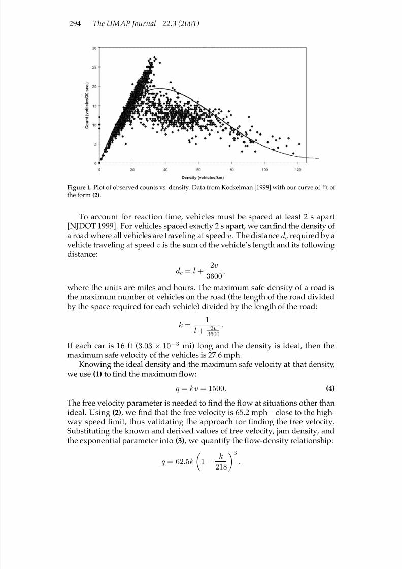
7/17/2019 UMAP 2001 vol. 22 No. 3



Figure 1. Plot of observed counts vs. density. Data from Kockelman [1998] with our curve of Þt of the form (2).

To account for reaction time, vehicles must be spaced at least 2 s apart[NJDOT 1999]. For vehicles spaced exactly 2 s apart, we can Þnd the density of a road where all vehicles are traveling at speed v. The distance dc required by avehicle traveling at speed v is the sum of the vehicle’s length and its followingdistance:

dc = l + 2v

3600,

where the units are miles and hours. The maximum safe density of a road is

the maximum number of vehicles on the road (the length of the road divided by the space required for each vehicle) divided by the length of the road:

k = 1

l + 2v3600

.

If each car is 16 ft (3.03 × 10−3 mi) long and the density is ideal, then themaximum safe velocity of the vehicles is 27.6 mph.

Knowing the ideal density and the maximum safe velocity at that density,we use (1) to Þnd the maximum ßow:

q = kv = 1500. (4)

The free velocity parameter is needed to Þnd the ßow at situations other thanideal. Using (2) , we Þnd that the free velocity is 65.2 mph—close to the high-way speed limit, thus validating the approach for Þnding the free velocity.Substituting the known and derived values of free velocity, jam density, andthe exponential parameter into (3) , we quantify the ßow-density relationship:

q = 62.5k

1− k

218

3.

7/17/2019 UMAP 2001 vol. 22 No. 3



TrafÞc Flow Model

Mapping the Region

We programmed in Java a simpliÞed map of South Carolina that consists of

107 junctions (cities) and 154 roads. A junction is an intersection point betweentwo or more roads. A road connects exactly two junctions. Our map includesmost of the roads in by SCEPD’s model and many more. Data for the numberof cars, boats, and campers in each city used in the computer model can befound in the Appendix. [EDITOR’S NOTE: We omit the Appendix.]

Behavior of Cities

Each point in the program stores a city’s population and regulates traf Þcßow into and out of the roads connected to it. First, it ßows cars out of the

city into each road. The desired ßow out—the maximum number of vehiclesthat the road can take—is deÞned by the ßow-density equation (4) for the roadthat the cars are entering. If the total number of vehicles that can be exitedexceeds the evacuee population of the city, then the evacuees are distributedproportionally among the roads with respect to the size of the road.

Next, the city lets vehicles in. The roads always try to ßow into the city atthe ideal ßow rate. The city counts the total number of cars being sent to it andcompares this to its current evacuee capacity. If the evacuee capacity is lessthan the number of vehicles trying to enter, the city accepts a proportion of thevehicles wanting to enter, depending on the road size. A check in the programensures that the number of vehicles taken from the road does not exceed the

number of cars on the road at that time.After repeating the entering and exiting steps for each road, the city recal-

culates its current evacuee population, removing all the vehicles that left andadding all the vehicles that entered.

Behavior of Roads

We deÞne each road by its origin junction, destination junction, length, andnumber of lanes. The number of lanes is the number of lanes in a certain direc-tion under nonemergency circumstances. For example, a road that normally

has one lane north and one lane south is considered a one-lane highway. If thenumber of lanes on a road changes between cities, we use the smaller numberof lanes. To analyze the possibility of turning both lanes to go only north oronly south, our program would double the number of lanes.

During an evacuation, traf Þc never needs to ßow in both directions, be-cause the net ßow of a road that ßowed equally in two directions would bezero. Therefore, each road has a direction deÞned by its origin junction anddestination junction. While the origin junction is normally the point closer to

7/17/2019 UMAP 2001 vol. 22 No. 3



the coast, the program analyzes the possibility of having the road ßow from its“destination” to “origin.” In some cases, this could provide the optimal ßowout of the coastal areas by Þnding alternative routes.

We model traf Þc congestion as a funnel. As long as vehicles are on theroad, they attempt to exit at the ideal ßow rate. However, if the road begins

to Þll, then the number of vehicles entering the road varies depending on theßow-density equation (4). We determine the new density of the road via

Di = ni + ∆ni

d ,

where ni is the initial number of vehicles on the road, ∆ni is the difference between the cars entered and cars exited, and d is the length of the road (mi).

Optimization Algorithm

We use a modiÞed genetic optimization algorithm, beginning from SouthCarolina’s current solution into the evacuation. The simulation stores a pos-sible solution as two chromosomes: a city chromosome, storing the time tostart evacuating coastal cities, and a road chromosome, storing directions andreversals of the roads. Stored with the solution is the number of people left inthe evacuation zone after 24 h, the usual advance notice for evacuation.

The simulation randomly chooses a chromosome and a gene to mutate. Weuse a uniform distribution to choose Þrst the chromosome, then the gene, andÞnally a value for that gene. City genes can take the value of any time step between 0 and 12 h before starting to evacuate. Road direction can be in either

the speciÞed direction, the reversed direction, or closed. Opposing lanes can be either reversed or not reversed. If the changed chromosome leaves fewerpeople in the evacuation region in 24 h, it replaces the old chromosomes.

Results

Knowing that the maximum ßow of a one-lane road is 1,500 cars per hour,weÞrsttested SouthCarolina’s currentevacuation routewith ourmodiÞedßowequations, which allow for more people to leave the evacuation region. After24 h, 556,000 people (58% of the people needing to leave) were still left in thecities needing evacuation. If only I-26 was reversed, the people left droppedto 476,000 (50%). However, if people were allowed to take their boats andcampers with them, the number left was 619,000. Therefore, boats, campers,and extra cars generally should not be allowed to evacuate.

After 10,000 iterations, the solutions were still improving. Therefore, werestarted the program with all roads beginning with lanes reversed and citiesevacuating immediately. After 10,000 iterations, the program could not Þnd a better solution than one in which 233,000 people (25%) are left.

7/17/2019 UMAP 2001 vol. 22 No. 3



If I-95 is too congested due to traf Þc from Georgia and South Carolina (i.e.,I-95 is not used in the simulation), the number of people left is 254,000, 9.4%more than if the highway had been clear.

IncreasingColumbia’sevacueecapacityhelpstheevacuationonlymarginally,removing only 948 more people from danger.

Regardless of the situation, the solutions always have cities that start evac-uating immediately: Staggered solutions are not optimal.

Stability Analysis

We tested the ßow equations in the evacuation simulation by varying theexponential parameter, the free velocity, and the jam density. When the ex-ponential parameter was increased or decreased by 1, the number of peopleevacuated changed by only 0.2% and 1.0%. Doubling or halving the free ve-locity caused variations of 3.4%. Doubling and halving the jam density caused

variations of 2.2%. The length of the car did not affect the number of peopleemptied from the city because the following distance was so large compared tothe length of the car. Finally, we doubled and halved the iterative time step of the evacuation simulation, which did not change number of people evacuated.Thus, this model was robust in every variable tested.


Strengths

• The model can be used for any evacuation. For, example, if a meteor werepredicted to hit the Atlantic Ocean and ßood a strip of land 50 mi wide alongthe Atlantic Coast, this model could be used to evacuate residents of SouthCarolina to areas not affected by the ßood.

• Moreover, the program is ßexible enough to work for any possible map; itis not speciÞc to the individual roads and cities of South Carolina.

• The model is stable with regards to all variables tested, and the optimizationalgorithm runs very quickly.

Weaknesses

• The greatest weakness of this model is that it assumes that people will followdirections: use the two-second following distance rule, travel at the speedlimit, and travel on assigned roads.

• The model assumes density homogeneity along each road after each itera-tion, while in reality the density varies.

7/17/2019 UMAP 2001 vol. 22 No. 3



• The model can handle only situations where the roads are empty at the beginning of the simulation.

• We underestimated the holding capacity of the cities, leading to a slower exitfrom the unsafe regions. Thus, although the relative changes in the resultsare probably correct, the actual number of people in danger after 24 hoursis probably fewer.

• The optimization algorithm can get stuck in local minima.

Conclusion

Reversing traf Þc on all evacuation routes evacuates the most people. Traf Þcfrom Georgia and Florida is not a problem, but many boats and campers wouldsigniÞcantly decrease ßow.

Hence, we suggest that roads be reversed and that to maintain maximumßow, traf Þc regulators not allow the numberof cars ina stretch of road to exceed54.4 per lane per mile, by regulating on- and off-ramps at cities.

References

Feigenbaum, Edward D., and Mark L. Ford. 1984. South Carolina Title 25,Chapter 1, Article 4. In Emergency Management in the States , 46. Council onState Governments.

Haynie, S.G. 2000. WWW Transportation Tutorial Site. North Carolina State

University.http://www.eos.ncsu.edu/eos/info/ce400_info/www2/flow1.html . Ac-cessed 12 February 2001.

Jayakrishnan, R., U. Rathi, C. Rindt, and G. Vaideeshwaran. 1996. Enhance-ments to a simulated framework for analyzing urban traf Þc networks withATIS/ATMS. PATH Research Report UCB-ITS-PRR-96-27 (October 1996).

Kockelman, K.M. 1998. Changes in the ßow-density relation due to environ-mental, vehicle, and driver characteristics. Transportation Research Record(Paper Number 980734) 1644: 47–56.

New Jersey Department of Transportation (NJDOT). 1999. 1999 Driver’s Man-ual. http://liberty.state.nj.us/mvs/dm99/99ch5c.htm\#Two .Accessed 12 February 2001.

Real-time GIS assists hurricane evacuation. 2000. American City and County(February 2000) 115 (2): 24.

South Carolina Emergency Preparedness Division, South CarolinaDepartmentof Public Safety. 1999. Evacuation Plan. http://www.dot.state.sc.us/getting/evacmid.html . Accessed 12 February 2001.

7/17/2019 UMAP 2001 vol. 22 No. 3



Vaccaro, Chris. 2000. 1999 hurricane season closes, sets records. USA Today.http://www.usatoday.com/weather/hurricane/1999/atlantic/

wrapup99.htm . Accessed 12 February 2001.

The Crowd Before the Storm:Improved Hurricane

Evacuation Routes Planned

Columbia, SC, Feb. 12—Anewmathematical model prepared for theSouth Carolina Emergency Prepared-

ness Division should end aggravatingand dangerous backups when a hurri-cane threatens South Carolina. In re-sponse to the monstrous traf Þc jamsthat turned I-26 northbound out of Charleston into a parking lot duringthe Hurricane Floyd evacuation, thenewmodel distributes traf Þcoversev-eral smaller routes.

One of the new program’s con-

troversial traf Þ

c-control methods is tomake all lanes of traf Þc on evacuationroutes to run in the same direction,away from the beach, to improve traf-Þc ßow.

People with campers, RVs, boats,and more than one car should leaveas early as possible if a hurricane ispredicted; once the new plan is im-plemented, families may be permittedonly one car, to reduce traf Þc.

Themodel counteracts these minorinconveniences by evacuating 75% of the population at risk within 24 hours,

compared to 42% under South Car-olina’s current plan.

Although more people may be

evacuated, don’t expect to get out of the region too quickly. The model pre-dicts that the fastest evacuation willoccur if all cars travel at 28 mph. Atthat rate, it will take you 4 hours to getout of the evacuation region.

The model used a “genetic algo-rithm” approach, which involves test-ing possible solutions against eachother and “breeding” new ones from

the best ones so far. Further anal-ysis showed that reversing lanes of all roads along the evacuation routesis the best method for quick evacua-tion. The computer tested 10,000 mi-nor changes without Þnding a moreeffective solution.

Increasing the housing and park-ingcapacityofColumbiabyconstruct-ing a shelter there would be onlymildly helpful. On a more positive

note, residents do not need to worryabout traf Þc from Georgia and Floridaslowing the evacuation.

— Jonathan David Charlesworth, Finale Pankaj Doshi, and Joseph EdgarGonzalez, in Richmond, Virginia.

7/17/2019 UMAP 2001 vol. 22 No. 3



7/17/2019 UMAP 2001 vol. 22 No. 3


Jammin’ with Floyd 301

Jammin’ with Floyd:

A TrafÞc Flow Analysis of South

Carolina Hurricane EvacuationChristopher HanusaAri NiehMatthew SchnaiderHarvey Mudd CollegeClaremont, CA

Advisor: Ran Libeskind-Hadas

Introduction

We analyze the 1999 Hurricane Floyd evacuation with a traf Þc-ßow model,explaining the extreme congestion on I-26. Then we look at the new SouthCarolinaHurricaneEvacuationPlan,whichincludeslanereversals. We analyzetheir effect; they would signiÞcantly beneÞt traf Þc leaving Charleston. Withlane reversals, the maximum number of vehicles passing any point on I-26 is6,000 cars/h.

We develop two plans to evacuate the South Carolina coast: the Þrst bygeographic location, the second by license-plate parity.

We explore the use of temporary shelters; we Þnd that I-26 has suf Þcientcapacity for oversized vehicles; and we determine the effects of evacuees fromGeorgia and Florida.

TrafÞc Flow Model

ThefollowingdeÞnitions andmodel are taken directly from Mannering andKilareski [1990, 168–182].

The primary dependent variable is level of service (LOS), or amount of

congestion, of a roadway. There are six different LOS conditions, A through F,with A being the least congested and F being the most congested. We focus onthe distinction between levels E and F.


7/17/2019 UMAP 2001 vol. 22 No. 3



• Level of Service E representsoperatingconditions at or near capacity level. Allspeeds are reduced to a low but relatively uniform value, normally between30 and 46 mph.

• Level of Service F is used to deÞne forced or breakdown ßow, with speedsof less than 30 mph. This condition exists wherever the amount of traf Þcapproaching a pointexceeds theamount that cantraverse that point. Queuesform behind such locations.

If we enter LOS F, the roadway has exceeded its capacity and the usefulnessof the evacuation has broken down. An evacuation strategy that results in ahighway reaching LOS F is unacceptable.

For a given highway, we can determine the maximum number of vehiclesthat can ßow through a particular section while maintaining a desired levelof service. To make this more concrete, we deÞne the characteristic quantitymaximum service ßow.

DeÞnition. MaximumServiceFlow (MSFi)foragivenlevelofservicei , assumingideal roadway conditions, is the maximum possible rate of ßow for a peak 15-min period, expandedto an hourly volume and expressed in passenger cars perhour per lane (pcphpl). To calculate the MSF of a highway for a given LOS, wemultiply the road’s capacity under ideal conditions by the volume-to-capacityratio for the desired LOS. More formally,

MSFi = cjv

c i, (1)

where cj is the capacity under ideal conditions for a freeway with DesignSpeed j , and (v/c)i is the maximum volume-to-capacity ratio associated with

LOS i. For highways with 60- and 70-mph design speeds, cj is 2,000 pcphpl[Transportation Research Board 1985]. Since LOS E is considered to be “atcapacity,” (v/c)E = 1.0. The design speed of a road is based mostly on theimportance and grade of the road; roads that are major and have shallowergrades have higher design speeds. The elevation proÞle along I-26 shows thatSouth Carolina is ßat enough to warrant the highest design speed.

An immediate consequence of (1) is that to maintain MSFE or better (whichwe consider necessary for a successful evacuation), the number of passengercars per hour per lane must not exceed 2,000 for any highway.

For it to be useful in model calculations, we need to convert the maximum

serviceß

ow to a quantity that conveys information about a particular roadway.This quantity is known as the service ßow rate of a roadway.

DeÞnition. The service ßow rate for level of service i , denoted SFi , is the actualmaximal ßow that can be achieved given a roadway and its unique set of prevailing conditions. The service ßow rate is calculated as

SFi = MSFiNf wf HVf p, (2)

in terms of the adjustment factors:

7/17/2019 UMAP 2001 vol. 22 No. 3



N : the number of lanes,

f w: the adjustment for nonideal lane widths and lateral clearances,

f HV: effect of nonpassenger vehicles, and

f p: the adjustment for nonideal driver populations.We assume that the lanes on I-26 and other highways are ideal (i.e., f w = 1): atleast 12 ft wide with obstructions at least 6 ft from traveled pavement [Manner-ingand Kilareski 1990]. To account for driverunfamiliarity with reversedlanesand stress of evacuation, we set f p = 0.7 for reversed lanes and f p = 0.8 fornormal lanes, in accordance with Mannering and Kilareski [1990]. The modelalso employs an adjustment factor, denoted f HV , for reduction of ßow due toheavy vehicles such as trucks, buses, RVs, and trailers. Later we discuss theeffects of heavy vehicles on traf Þc ßow.


This model is easy to implement, the mathematics behind it is quite sim-ple, and it is backed by the National Transportation Board. We establish itsreliability by using it to predict traf Þc ßow patterns in the 1999 evacuation.

We assume that the number of lanes does not change, which requires thatthere are no lane restrictions throughout the length of the freeway and no lanesare added or taken away by construction.

The major weakness of our model is that it fails to take into account theerratic behavior of people under the strain of a natural disaster.

The simplicity of our model also limits its usefulness. It can be applied onlyto normal highway situations, not to a network of roads.

Improving Evacuation Flow

Gathering data from a various sources, we estimate the number of vehi-cles used in the 1999 evacuation. According to Dow and Cutter [2000], 65% of households that were surveyed chose to evacuate. About 70% of householdsused one vehicle or fewer, leaving 30% of households taking two vehicles. Of

the evacuees, 25% used I-26 during the evacuation. Based on population esti-mates [County Population Estimates . . . 1999] and average number of peopleper household [Estimates of Housing Units . . . 1998], and assuming a rela-tively uniform distribution of people per household, we calculate the numberof vehicles used during the evacuation (Table 1).

7/17/2019 UMAP 2001 vol. 22 No. 3



Table 1.

Evacuation participation estimates for Hurricane Floyd, in thousands.

Population Evacuees Evacuating Vehicles VehiclesHouseholds on I-26

Southern 187 122 47 61 —

Central 553 359 139 181 —Northern 233 152 59 76 —

Total 973 632 245 319 61

Reversing Lanes

According to our model, the capacity of a highway is directly proportionalto the number of lanes. This implies that lane reversal would nearly doublethe capacity of I-26.

Approximately 319,000 vehicles were used to evacuate the coastal countiesof South Carolina. Of evacuees surveyed by Dow and Cutter [2000], 16.3%evacuated between noon and 3 p.m. on Sept. 14. Assuming independence between the above factors, in the hours between 9 a.m. and noon, I-26 musthave been clogged by an attempted inßux of about 3,300 vehicles/h. Evenif evenly distributed, this was more than the 3,200 vehicles/h that the twoColumbia-bound lanes of I-26 could take under evacuation conditions. Theresult was LOS F—a large traf Þc jam. Our model predicts that this jam wouldhave lingered for hours, even after the inßux of vehicles had died down.

What if the coastal-bound lanes of I-26 were reversed? With corrections fornonideal conditions, our model predicts an SFE of 6,000 pcphpl. Therefore,

reversing the lanes of I-26 has the potential to increase service ß

ow rate by afactor of 1.6.

Simultaneous Evacuation Strategies

By Hurricane PathHurricanes sweep from south to north. Because a hurricane commonly

travels at a speed of less than 30 mph, the southernmost counties of SouthCarolina would be affected at least two hours before the northernmost ones.

However, analysis indicates that a staggered evacuation strategy would not

improve the speed of the evacuation. The evacuation routes are largely par-allel to one another and rarely intersect. Thus, the evacuation of each countyshould affect only the traf Þc on evacuation routes of nearby counties. There-fore, postponing evacuation of counties farther from the hurricane would becounterproductive.

7/17/2019 UMAP 2001 vol. 22 No. 3



By CountyWhat about avoiding simultaneous evacuation of adjacent counties? We

recommend evacuating Jasper, Beaufort, Charleston, Georgetown, and Horrycounties in the Þrst wave, and leaving Hampton, Colleton, Dorchester, andBerkeley until 3–6 h later, depending on the time of day. This solution would

decrease the probability of traf Þc reaching LOS F on any highway withoutsigniÞcantly delaying the evacuation. The nearby state of Virginia has a similarplan for evacuating county by county [Virginia Hurricane . . . 1991].

By License Plate NumberBy dividing cars into two categories, depending on the parity of the last

digit on their license plate, we could separate traf Þc into two waves withoutgiving preference to residents of any county. Our solution would request thatthe even group evacuate 3–6 h after the odd group was given the evacuationorder. This would spread out the hours of peak evacuation traf Þc, resulting

in improved traf Þc conditions and decreased risk of LOS F being reached. Acomparison of Figures 1 and 2 demonstrates the change in time distributionof evacuation when half of the drivers evacuate six hours later. Clearly, thedistribution is much smoother, reducing the likelihood of reaching LOS F.

Figure 1. Hurricane Floyd: Fraction of evacuating population vs. hours after the 1999 mandatoryevacuation order. (Data from Dow and Cutter [2000].)

Figure 2. Even/odd license plate plan: Our projected fraction of the evacuating population vs.hours after the mandatory evacuation order.

7/17/2019 UMAP 2001 vol. 22 No. 3



Lane Reversal on Smaller Highways

As only 29% of evacuees took I-26 or I-95, the majority took smaller roadsinland. Because our model results in linear growth of ßow with number of available lanes, lane reversals should improve evacuation rates on all roads.Because the evacuation routes are nearly perpendicular to the coastline, thereis little risk of opposing traf Þc being disrupted by these reversals. The logisticsof such an action, however, might be prohibitive.

The number of personnel needed to facilitate the I-26 lane reversal is 206[South Carolina Emergency Preparedness Division 2000]. Smaller highwayshave less distance between exits, which suggests that more personnel per milewould be needed to blockade highway entrances. The total length of highwayon all evacuation routes is approximately ten times as great as the length of I-26. Therefore, a truly prodigious amount of human effort would be necessaryto implement lane reversals on all evacuation routes.

It would be imprudent to spend resources for what we estimate to be only

a marginal gain in actual highway use. According to Dow and Cutter [2000],these alternative routes did not even approach capacity during the last evacua-tion. Since our license-plate evacuation strategy increases the overall through-put of major evacuation routes through lane reversal and smoother time distribution, there is no reason to expect a heavier load on state and country roads.

So, there is little evidence to support the utility of lane reversal on all smallerroads. Still, reversing laneson a small number of evacuation routes mightproveuseful. The three major population centers of the coast (Beaufort, Charleston,and Horry counties) have different evacuee distributions. Therefore, thosehighways which most merit reversalare I-26, I-501 fromMyrtleBeach toMarionand 301 from Marion to Florence, and the southern corridor from Beaufort

County to the Augusta area.

Effect of Additional Temporary Shelters

In 1999, South Carolina housed about 325,000 people in shelters [Dow andCutter 2000]. In a hurricane, one-third of evacuees go to each of shelters, familyand friends, and commercial establishments [Zelinski and Kosinski 1991, 39–44]. According to South Carolina Hurricane Information [2001], the numberof predesignated shelters in Columbia is insigniÞcant. However, there must be an ef Þcient way to funnel the evacuees to the evacuation sites, such as a

central coordination center with an up-to-date list of where the next group of cars should go.

Vehicle Type Restrictions

Although our model generally calculates ßow using only normal passengercars, it is not dif Þcult to take other types of vehicles into account. The equation

7/17/2019 UMAP 2001 vol. 22 No. 3



used to calculate the heavy-vehicle adjustment factor is

f HV = 1

1 + 0.6P , (3)

where P is the proportion of nonpassenger vehicles (RVs, trailers, and boats).

Using this equation, our model predicts an upper bound on the proportionof nonpassenger vehicles that occur without causing LOS F. We demonstratethis with a sample calculation using I-26. Earlier, we estimated the SFE of I-26,includingreversed lanes, as 6,000pcphpl. We also estimatedthat a maximum of 3,300 vehicles/h would enter I-26, ignoring the possibility of spikes in activity.Therefore, the minimum safe value of f HV is approximately 0.55 , which meansthat I-26 has enough leeway to support any mix of passenger cars and heavyvehicles. There is no need to restrict large vehicles on I-26.

Georgians, Floridians, and the I-95 CorridorAccording to Georgia’s hurricane evacuation plan [Hurricane EvacuationRoutes 2001], I-95 is not a valid evacuation route. However, thousands of Floridians and Georgians ßocked north on I-95 during Hurricane Floyd. InSavannah, the most popular evacuation route was I-16, which goes directlyaway from South Carolina [Of Þcials deserve high marks . . . 1999]. In SouthCarolina, as shown in Figures 1 and 2 , the farther away the destination, thesmaller the percentage of the evacuee population that plans to go there. Takingall this into account, a realistic upper bound for the percentage of Georgians orFloridians using I-95 is 20%.

Any population entering South Carolina on I-95 from Georgia or Florida ismostly bound for major cities; an upper bound on the traf Þc headed throughColumbia would be 75%. Since Floyd’s landfall was extraordinarily unpre-dictable, we propose that it was one of the largest evacuations that will affectSouth Carolina.

Our reasoning is as follows: Hurricanes of lesser strength have fewer evac-uees. If the landfall of the hurricane is more southerly, there is less need toevacuate South Carolina and North Carolina and so there will be less traf Þc onthe I-26. Lastly, if the hurricane tends more towards the north, the number of evacuee drivers from Georgia and Florida taing I-95 will be decreased greatly.So, we can take Floyd as a relative upper bound on evacuees.

From CNN’s coverage of the lead up to Hurricane Floyd’s landfall, in Geor-gia, we know that “the evacuation orders affected 500,000 people.” We boundthis rough estimate by 600,000. So the upper bound of people using I-95 can beestimated as (0.20)(0.75)(600,000) ≈ 90,000 , or about 45,000 vehicles, spreadover a two-day period. From Dow and Cutter [2000], we know that about 10%of South Carolina evacuees used I-95, so the Georgians and Floridians effec-tively doubled the traf Þc on I-95, which is a huge impact on the model that wehave proposed.

7/17/2019 UMAP 2001 vol. 22 No. 3



Improvements in the Model

Ourmodel needs additional evacuation data. With precise statistics regard-ingnumber of evacuees, routes taken, time distributions, andtraf Þc conditions,we could apply it to a greater variety of situations.

Additional reÞnements might be made to the parameters of the model withinformation on the highways themselves. The lane widths and distances toroadside obstacles affect the service ßow rate, and knowing the exact layout of the highways would enable us to take them into account.

We could also use information regarding the resources available to thestate:how many personnel and vehicles would be available to run lane reversals.

With suf Þcient information, we could use this model to create a simulationof a hurricane evacuation. We would treat the highways of South Carolina asedges in a network ßow problem and run a discrete computer simulation totest our premises and conclusions regarding evacuation policies.

References

County Population Estimates for July 1, 1999. 1999. http://www.census.gov/population/estimates/county/co-99-1/99C1_45.txt .

Dow, K., and S.L. Cutter. 2000. South Carolina’s Response to Hurricane Floyd.Quick Response Report 128. Columbia, SC: University of South Carolina.http://www.colorado.edu/hazards/qr/qr128/qr128.html .

Estimates of Housing Units, Households, Households by Age of Householder,

and Persons per Household: July 1, 1998. 1999. http://www.census.gov/

population/estimates/housing/sthuhh1.txt .

Floyd bashes Bahamas, takes aim at Florida. 1999. http://www.cnn.com/WEATHER/9909/14/floyd.07/ .

Gartner, Nathan, Carroll J. Messer, and Ajay K. Rathi. 1992. Traf Þc Flow Theory:A State of the Art Report. Revised monograph. Special Report 165. Oak Ridge, TN: Oak Ridge National Laboratory. http://www.tfhrc.gov/its/tft/tft.htm .

HurricaneEvacuationRoutes—TextForm. 2001. http://www.georgia-navigator.com/hurricane/textroutes.html .

Mannering, F., and W. Kilareski. 1990. Principles of Highway Engineering andTraf Þc Analysis. New York: Wiley.

Number of Households in South Carolina by County: 1950–1990 and Projected1995. 1996. http://www.sciway.net/statistics/scsa96/hou/hou13.html .

Of Þcials deserve high marks for handling of Hurricane Floyd threat. 1999.http://www.onlineathens.com/stories/091999/ope_0919990026.shtml .

7/17/2019 UMAP 2001 vol. 22 No. 3



PublicRoads. 1999. http://www.tfhrc.gov/pubrds/janfeb99/traffic.htm .

South Carolina Emergency Preparedness Division. 2000. Traf Þc ManagementCentral Coastal Conglomerate Annex I-26 Lane Reversal Operation Plan.Formerly available at http://www.state.sc.us/epd/hurricaneplan/ccci26rev.pdf ; now at http://www.cs.hmc.edu/~matt/ccc.pdf .

South Carolina Hurricane Evacuation Routes. 2001. http://www.dot.state.sc.us/getting/evacuationmap.pdf .

South Carolina Hurricane Information. 2000.http://www.scan21.com/selectcounty.html .

South Carolina Population Density. 1999. http://www.callsouthcarolina.com/Maps/Map-Pop_Density.htm .

Total Number of Housing Units by County: 1970, 1980 and 1990. 1999.http://www.ors.state.sc.us/abstract_99/chap12/hou3.htm .

Transportation ResearchBoard. 1985. Highway Capacity Manual. Special Report209.

Virginia Hurricane Evacuation Routes. 1991. http://www.vdot.state.va.us/traf/hurricane.html .

Zelinsky, Wilbur, and Leszek A. Kosinski. 1991. The Emergency Evacuationof Cities: A Cross-National Historical and Geographical Study. Savage, MD:Rowman and LittleÞeld.

Maurice Knocks on Door, No One Home

Columbia, S.C. (AP)— Hurri-cane season has come with a fury hereto South Carolina, where HurricaneMaurice, the 13th named storm of theseason, bears down on Charleston thisevening. A record 80% of the popula-tion has been evacuated through thenew evacuation plan.

When Hurricane Floyd narrowlymissed South Carolina in 1999, thelack of preparedness foran evacuationof such a magnitude was highly evi-dent. The state government asked theResearch All Day Corporation (RADCorp.) to come up with a new evacu-ation plan that would help the coastalresidents escape the ferocity of a simi-lar storm.

The RAD Corporation’s team of world-classhurricaneexpertsandtop-notch traf Þc engineers analyzed thesituation and developed a new evacu-ation plan. “The basic idea of the planstems from simple math,” explainedDr. K. Esner, Director of RAD Mod-eling. “Two sets of two lanes almostdoubles the evacuation rate.”

When asked to explain further,Dr. Esner continued, “On I-26, wherethere was a colossal traf Þcjamin1999,we decided to reverse the ßow of thecoastal-bound lanes at the Þrst deci-sion of a mandatory evacuation.” Inthis way, people leaving Charleston,the most populous city in South Car-olina, could take eitherthenormal two

7/17/2019 UMAP 2001 vol. 22 No. 3



lanes of I-26 or the two “contra-ßow”(reversed) lanes of I-26 all the way toColumbia.

The evacuees in the manyColumbia shelters seemed in good

spirits. There was much less traf Þc-related annoyance than was felt in1999. John C. Lately, a British residentof Myrtle Beach, joked, “You realizethat in England, driving on the left iscommonplace; I felt right at home.”

There was nothing but praise forthe RAD engineers. “A remarkabledifference was seen between the chaosof evacuating for hurricane Floydin 1999 and the evacuation today,”

said Joseph P. Riley, Jr., mayor of Charleston. “This time, the drive be-tween Charleston and Columbia took 4 hours instead of 18. And it’s a goodthing, too; this time the storm didn’tmiss.”

Another feature of thenew evacua-tion plan was the breakup of the evac-uating public into two groups. “Oneof our concerns about the 1999 Floyd

evacuation was the volume of cars alltrying to access the emergency roadsat thesame time,” explainedDr. Esner.He continued, “To alleviate the traf Þcvolumepressure, we wantedto dividethe population into two groups. Wehad two different proposals; we could break up the population geograph-

ically or basically divide the popu-lation right down the middle, usingeven/odd license plate numbers.”

With the proposed RAD plan, peo-ple with even license plates left in the

Þrst group, right when the evacua-tion order was given, and people withodd license plates or vanity plates leftstarting 6 hours later. “I thought theplanwascrazy,” remarkedCharles Or-ange, a 24-year-old Charleston resi-dent. “They told us to evacuate by li-cense plate number; you’d never think high school math would help you oneday, but this is one time it did!” heexclaimed.

Using the 1999 data, the RAD re-searchers calculated that breaking theevacuating population into two equalgroups and delaying one group by 6hours led to a condition where the vol-ume of cars at no time exceeded themaximum volume that the road couldhandle. In this way, therewasnoprob-lem with traf Þc jams, and Charleston became a ghost town, safe for Maurice

to make its appearance.The majority of the people left onthe beaches are surfers and media, buteven they are sparse in number; allthat remains is a hurricane without anaudience.

Hurricane Maurice could not bereached for comment.

— Christopher Hanusa, Ari Nieh, Matthew Schnaider, in Claremont, Calif.

7/17/2019 UMAP 2001 vol. 22 No. 3


Blowin’ in the Wind 311

Blowin’ in the Wind

Mark WagnerKenneth Kopp

William E. KolasaLawrence Technological UniversitySouthÞeld, MI

Advisor: Ruth G. Favro

Introduction

We present a model to determine the optimal evacuation plan for coastal

South Carolina in the event of a large hurricane. The model simulates theßow of traf Þc on major roads. We explored several possible evacuation plans,comparing the time each requires.

Traf Þc ßow can be signiÞcantly improved by reversing the eastbound lanesof I-26 from Charleston to Columbia. By closing the interchange between I-26and I-95 and restricting access to I-26 at Charleston, we can reduce the overallevacuation time from an original 31 h to 13 h.

However, a staggered evacuationplan,whichevacuatesthe coastlinecounty by county, does not improve the evacuation time, since traf Þc from each coastalpopulation center interferes little with traf Þc ßowing from other areas beingevacuated. Although reversing traf Þc on other highways could slightly im-

prove traf Þc ßow, it would be impractical. Restrictions on the number andtypes of vehicles could speed up the evacuation but would likely cause moreproblems than improvements.

Theory of TrafÞc Flow

We require a model that simulates traf Þc ßow on a large scale rather thanindividual carmovement. We take formulas to model traf Þcßow from Beltrami[1998]. Although traf Þc is not evenly distributed along a segment of road, it

can be modeled as if it were when large segments of road are being considered.We can measure the traf Þc density of a section of road in cars/mi. The traf Þc

TheUMAPJournal22 (3)(2001)311–321. cCopyright 2001 by COMAP, Inc. All rights reserved.Permission to make digital or hard copies of part or all of this work for personal or classroom useis granted without fee provided that copies are not made or distributed for proÞt or commercialadvantage and that copies bear this notice. Abstracting with credit is permitted, but copyrightsfor components of this work owned by others than COMAP must be honored. To copy otherwise,to republish, to post on servers, or to redistribute to lists requires prior permission from COMAP.

7/17/2019 UMAP 2001 vol. 22 No. 3



speed u at a point on the road can be calculated from the density according tothe formula

u(r) = um

1− ρ

ρm

,

where ρ is the traf Þc density, um is the maximum speed of any car on the road,

and ρm is the maximum traf Þc density (with no space between cars). We deÞnethe ßow of traf Þc at a point on the road as the number of cars passing that pointin a unit of time. The ßow q can be easily calculated as

q (ρ) = ρu.

It is the ßow of traf Þc that we desire to optimize, since greater ßow results in agreater volume of traf Þc moving along a road.

Assumptions

• During an evacuation, there is an average of 3 people per car. This is rea-sonable, since people evacuate with their entire families, and the averagehousehold in South Carolina has 2.7 people, according to the 1990 census.

• The average length of a car on the road is about 16 ft.

• In a traf Þc jam, there is an average of 1 ft of space between cars.

• The two above assumptions lead to a maximum traf Þc density of

5280 ft/mile

17 ft/car = 310 cars/mile/lane.

• The maximum speed is 60 mph on a 4-lane divided highway, 50 mph on a2-lane undivided country road.

• Vehicles follow natural human tendencies in choosing directions at intersec-tions, such as preferring larger highways and direct routes.

• The traf Þc ßow of evacuees from Florida and Georgia on I-95 is a continuousstream inward to South Carolina.

• When vehicles leave the area of the model, they are considered safely evac-uated and no longer need to be tracked.

• There will not be traf Þc backups on the interstates at the points at which theyleave the area of the model.

• A maximum of 30 cars/min can enter or exit a 1-mi stretch of road in a pop-ulated area, by means of ramps or other access roads. Up to the maximumexit rate, all cars desiring to exit a highway successfully exit.

7/17/2019 UMAP 2001 vol. 22 No. 3



• The weather does not affect traf Þc speeds. The justiÞcations are:

– During the early part of the evacuation, when the hurricane is far fromthe coast, there is no weather to interfere with traf Þc ßowing at themaximum speed possible.

– During the later part of the evacuation, when the hurricane is approach-ing the coast, traf Þc ßows suf Þciently slowly that storm weather wouldnot further reduce the speed of traf Þc.

• There is suf Þcient personnel available for any reasonable tasks.

Objective Statement

We measure the success of an evacuation plan by its ability to evacuateall lives from the endangered areas to safe areas between announcement of

mandatory evacuation and landfall of the hurricane; the best evacuation plantakes the shortest time.

Model Design

The TrafÞc Simulator

Our traf Þc simulator is based on the formulas above. Both space and timeare discretized, so that the roads are divided into 1-mi segments and time isdivided into 1-min intervals. Vehicles enter roads at on-ramps in populatedareas, leave them by off-ramps, and travel through intersections to other roads.

Each 1-mi road segment has a density (the number of cars on that segment),a speed (mph), and a ßow (the maximum number of cars that move to thenext 1-mile segment in 1 min). Each complete road section has a theoreticalmaximum density ρm and a practical maximum density ρm (accounting for 1 ftof space between cars), which can never be exceeded.

Moving TrafÞc Along a Single Road

The ßow for each road segment is calculated as

q (ρ) = ρu

um.

If the following road segment is unable to accommodate this many cars, theßow is the maximum number of cars that can move to the next segment.

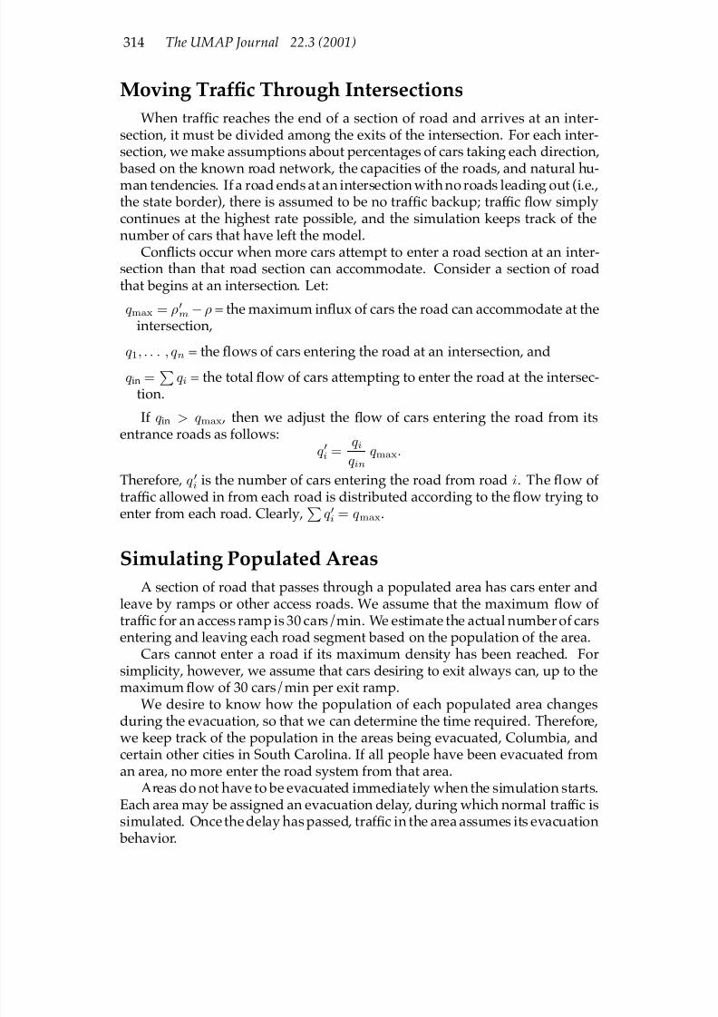
7/17/2019 UMAP 2001 vol. 22 No. 3



Moving TrafÞc Through Intersections

When traf Þc reaches the end of a section of road and arrives at an inter-section, it must be divided among the exits of the intersection. For each inter-section, we make assumptions about percentages of cars taking each direction, based on the known road network, the capacities of the roads, and natural hu-man tendencies. If a road ends at an intersection with no roads leading out (i.e.,the state border), there is assumed to be no traf Þc backup; traf Þc ßow simplycontinues at the highest rate possible, and the simulation keeps track of thenumber of cars that have left the model.

Conßicts occur when more cars attempt to enter a road section at an inter-section than that road section can accommodate. Consider a section of roadthat begins at an intersection. Let:

q max = ρm−ρ = the maximum inßux of cars the road can accommodate at theintersection,

q 1, . . . , q n = the ß

ows of cars entering the road at an intersection, andq in =

q i = the total ßow of cars attempting to enter the road at the intersec-

tion.

If q in > q max , then we adjust the ßow of cars entering the road from itsentrance roads as follows:

q i = q iq in

q max.

Therefore, q i is the number of cars entering the road from road i. The ßow of traf Þc allowed in from each road is distributed according to the ßow trying toenter from each road. Clearly, q i = q max.

Simulating Populated Areas

A section of road that passes through a populated area has cars enter andleave by ramps or other access roads. We assume that the maximum ßow of traf Þc for an access ramp is 30 cars/min. We estimate the actual number of carsentering and leaving each road segment based on the population of the area.

Cars cannot enter a road if its maximum density has been reached. Forsimplicity, however, we assume that cars desiring to exit always can, up to themaximum ßow of 30 cars/min per exit ramp.

We desire to know how the population of each populated area changesduring the evacuation, so that we can determine the time required. Therefore,we keep track of the population in the areas being evacuated, Columbia, andcertain other cities in South Carolina. If all people have been evacuated froman area, no more enter the road system from that area.

Areas do not have to be evacuated immediately when the simulation starts.Each area may be assigned an evacuation delay, during which normal traf Þc issimulated. Once the delay has passed, traf Þc in the area assumes its evacuation behavior.

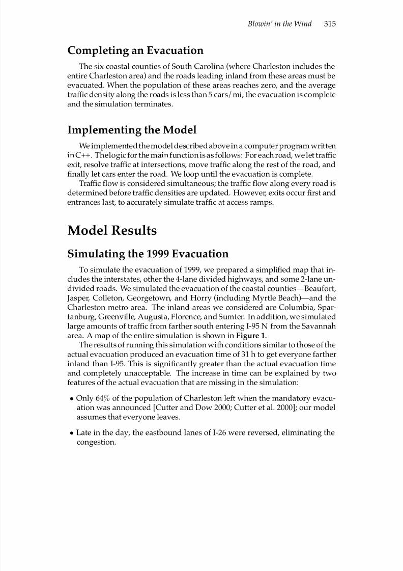
7/17/2019 UMAP 2001 vol. 22 No. 3



Completing an Evacuation

The six coastal counties of South Carolina (where Charleston includes theentire Charleston area) and the roads leading inland from these areas must beevacuated. When the population of these areas reaches zero, and the averagetraf Þc density along the roads is less than 5 cars/mi, the evacuation is completeand the simulation terminates.

Implementing the Model

We implementedthemodel describedabove in a computerprogram writteninC++. Thelogic for the mainfunction isas follows: For each road, welet traf Þcexit, resolve traf Þc at intersections, move traf Þc along the rest of the road, andÞnally let cars enter the road. We loop until the evacuation is complete.

Traf Þc ßow is considered simultaneous; the traf Þc ßow along every road isdetermined before traf Þc densities are updated. However, exits occur Þrst and

entrances last, to accurately simulate traf Þc at access ramps.

Model Results

Simulating the 1999 Evacuation

To simulate the evacuation of 1999, we prepared a simpliÞed map that in-cludes the interstates, other the 4-lane divided highways, and some 2-lane un-divided roads. We simulated the evacuation of the coastal counties—Beaufort,

Jasper, Colleton, Georgetown, and Horry (including Myrtle Beach)—and theCharleston metro area. The inland areas we considered are Columbia, Spar-tanburg, Greenville, Augusta, Florence, and Sumter. In addition, we simulatedlarge amounts of traf Þc from farther south entering I-95 N from the Savannaharea. A map of the entire simulation is shown in Figure 1.

The results of running this simulation with conditions similar to those of theactual evacuation produced an evacuation time of 31 h to get everyone fartherinland than I-95. This is signiÞcantly greater than the actual evacuation timeand completely unacceptable. The increase in time can be explained by twofeatures of the actual evacuation that are missing in the simulation:

• Only 64% of the population of Charleston left when the mandatory evacu-ation was announced [Cutter and Dow 2000; Cutter et al. 2000]; our modelassumes that everyone leaves.

• Late in the day, the eastbound lanes of I-26 were reversed, eliminating thecongestion.

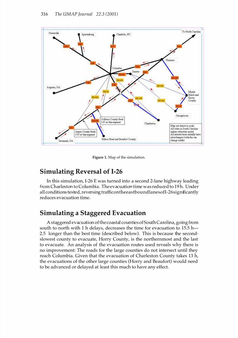
7/17/2019 UMAP 2001 vol. 22 No. 3



Figure 1. Map of the simulation.

Simulating Reversal of I-26

In this simulation, I-26 E was turned into a second 2-lane highway leadingfrom Charleston to Columbia. Theevacuation time was reduced to 19 h. Underallconditions tested, reversing traf ÞcontheeastboundlanesofI-26signiÞcantlyreduces evacuation time.

Simulating a Staggered Evacuation

A staggered evacuation of thecoastal countiesof South Carolina,goingfromsouth to north with 1 h delays, decreases the time for evacuation to 15.5 h—2.5 longer than the best time (described below). This is because the second-slowest county to evacuate, Horry County, is the northernmost and the lastto evacuate. An analysis of the evacuation routes used reveals why there isno improvement: The roads for the large counties do not intersect until theyreach Columbia. Given that the evacuation of Charleston County takes 13 h,the evacuations of the other large counties (Horry and Beaufort) would needto be advanced or delayed at least this much to have any effect.

7/17/2019 UMAP 2001 vol. 22 No. 3



Reversing Other Highways

Reversing traf Þc on smaller highways might improve traf Þc ßow, but thisis not a practical option. None of the roads besides I-26 is a controlled-accessroad; therefore, it is impossible to ensure that the traf Þc entering the reversedlanes would all move in the desired direction. A single vehicle entering andattempting to travel in the undesired direction would cause a massive jam.

The possible minor highways to Columbia that could be reversed are U.S.highways 321, 176, 521, 378, 501, and 21. All are non-controlled-access roads,meaning that there are no restrictions on where vehicles may exit or enter.Together, they have 450 mi of roadway. A quick examination of U.S. 501, thehighest-capacity of these, reveals two intersections per mile with other roads.Considering this as typical, there are 900 intersections outside of towns thatwould need to be blocked. Factoring in the no fewer than 60 towns along theway, the blocking becomes prohibitive.

Therefore, reversal of minor highways leading inland is not feasible. The

only road that can be feasibly reversed is I-26.

Adding Temporary Shelters to Columbia

According to our simulation, the population of the Columbia area after theevacuation (in the best-case scenario) was 1,147,000, a massive number abovethe 516,000 permanent residents. If more temporary shelters were establishedin Columbia, there would be less traf Þc leaving the city and therefore morecongestion within the city. This would reduce the rate at which traf Þc couldenter Columbia and lead to extra traf Þc problems on the highways leading into

it. The effect of this congestion is beyond our computer simulation.We investigated buildings for sheltering evacuees. Using smartpages.comto search for schools, hotels, and churches in the Columbia area, we found thenumbers of buildings given in Table 1. We assumed an average capacity foreach type of building. According to the table, Columbia can shelter 1,058,251;this leaves a deÞcit of 89,000.

Table 1.

Post-evacuation sheltering in the two counties (Richland and Lexington) that Columbia occupies.

Buildings People shelteredType in Richland in Lexington Total Per building Number

Permanent residents 516,251Schools—general * 83 113 196 900 176,400Hotels/motels 80 32 112 500 56,000Churches 568 386 954 250 238,500Schools—other** 63 16 79 900 71,100

Total 1,058,251

*We assume that schools average 600 students and can shelter 900.**Includes academies but excludes beauty schools, trade schools, driving schools, etc.

7/17/2019 UMAP 2001 vol. 22 No. 3



However, Charlotte NC had only a very small increase in population due toevacuation (from 396,000 to 411,000). The people that Columbia cannot sheltercan easily Þnd shelter in Charlotte.

Restricting Vehicle Types and Vehicle NumbersRestrictions on numbers and types of vehicles would indeed increase the

speed of the evacuation. However, there are no reliable ways to enforce suchrestrictions. Consider the following arguments:

• Forbidding camper vehicles may be unsuccessful, since for a sizable fractionof tourists the camper is their only vehicle.

• Restricting the number of vehicles to one per family:

– The record-keeping involved would be prohibitive.

– For some families, more than one vehicle is needed to carry all of thefamily members.

The I-95 TrafÞc Problem

We assume that if the interchange is not closed, at least 75% of the peoplecoming up from Florida and Georgia on I-95 will take I-26 to Columbia. This is because the next major city reachable from I-95 is Raleigh, 150 mi further on. Inour simulation, not closing this intersection (but keeping the eastbound lanesof I-26 reversed) increases the evacuation time to 19 h.

The Best Simulated Evacuation Plan

By altering various model parameters, we reduced the overall evacuationtime to 13 h:

• Reverse the eastbound lanes of I-26.

• Close the exit on I-95 N leading to I-26 W.

• Limit the ßow of traf Þc from Charleston to I-26 W.

Thethird item is necessary to reduce congestion along I-26 in theCharlestonarea. If too many cars are allowed on, the speed of traf Þc in Charleston dropssigniÞcantly. Although this unlimited access results in a greater average speedon the section of I-26 between Charleston and the I-95 interchange, the slow-downintheCharlestonareaisexactlythetypeofbackupthatcausedcomplaintsin 1999 and resulted in a greater total time to evacuate the city.

7/17/2019 UMAP 2001 vol. 22 No. 3



Conclusions

It is possible to evacuate coastal South Carolina in 13 h. Assuming that ahurricane watch is issued 36 h prior to landfall, the state can allow an ampledelay between voluntary evacuation announcement and a subsequent manda-

tory order. However, state agencies must take considerable action to ensurethat the evacuation will go as planned:

• Close the interchange between I-26 and I-95. Traf Þc on I-26 must remain onI-26; traf Þc on I-95 must remain on I-95.

• The two eastbound lanes of I-26 must be reversed immediately upon themandatory evacuation order.

• In Charleston, restrict entrance to I-26 to 15 cars/min at each entrance ramp.

Everyone in the areas to evacuate must be notiÞed. Within South Carolina, the

existing Emergency Alert System includes many radio stations that can informthe public of the incoming hurricane, the steps to take during evacuation, andwhich roads to use.

Residents must be more convinced to evacuate than they were during Hur-ricane Floyd. Appropriate measures must be taken to ensure that residentsevacuate and evacuate far enough inland.

Model Strengths and Weaknesses

StrengthsThe model’s predictions have a number of features found in a real evacua-

tion or other high-density traf Þc ßow:

• Aninitialcongestedareaaroundtheentrancerampsgiveswaytoahigh-ßowarea when there is no entering traf Þc.

• Overall traf Þc speed in high-ßow areas is around 35 mph.

• Merging traf Þc causes a major decrease in ßow.

WeaknessesThe model does not take into account

• city streets , which are important in moving people from the highways toshelter in Columbia.

• accidents. A single accident or breakdown could result in several hours of delay. Tow trucks should be stationed at regular intervals along major roads.

7/17/2019 UMAP 2001 vol. 22 No. 3



• local trafÞc on thenon-controlled-accesshighways , which would slow traf-Þc on those roads.

References

Beltrami, Edward. 1998. Mathematics for Dynamic Modeling. 2nd ed. San Diego,CA: Academic.

City of Myrtle Beach: Frequently Asked Questions. 2000.http://www.cityofmyrtlebeach.com/faq.html . Accessed 12 February2001.

Compton’s Encyclopedia Online, vol. 3.0. South Carolina.http://www.comptons.com/encyclopedia/ARTICLES/0150/01710336_A.

html . The Learning Company., Inc. Accessed 12 February 2001.

Cutter, Susan L., and Kirstin Dow. 2000. University of South Carolina: Quick Response Report 128: South Carolina’s Response to Hurricane Floyd.http://www.cla.sc.edu/geog/hrl/Quick%20Response%20Report.htm .Accessed 12 February 2001.

, Robert Oldendick, and Patrice Burns. 2000. University of South Car-olina: Preliminary Report 1: South Carolina’s Evacuation Experience withHurricaneFloyd. http://www.cla.sc.edu/geog/hrl/Floyd_evacuation.html . Accessed 10 February 2001.

Emergency Response Planning and Management, Inc. 2000. Assessment of South Carolina’s experience with the 1999 hurricane season. http://www.

state.sc.us/epd/HurrBrief.pdf . Accessed 9 February 2001.

Rand McNally Road Atlas: United States, Canada, Mexico. 1995. Skokie, IL: RandMcNally & Company.

smartpages.com .

South Carolina Asset Network. http://www.scan21.com/hurricane_main.html . Accessed 9 February 2001.

U.S. Army: Hurricane/Tropical Storm ClassiÞcation Scale. http://www.sam.usace.army.mil/op/opr/hurrclss.htm . Accessed 10 February 2001.

U.S. Census Bureau: South Carolina ProÞles (from the 1990 census). http://www.census.gov/datamap/www/45.html . Accessed 10 February 2001.

U.S. Census Bureau: Georgia ProÞles (from the 1990 census). http://www.census.gov/datamap/www/13.html . Accessed 12 February 2001.

7/17/2019 UMAP 2001 vol. 22 No. 3



Students Develop Optimal

Coastal Evacuation Plan

Southfield, Mich., Feb. 12—During September 13–15, 1999, Hurri-cane Floyd threatened landfall alongthe coast of South Carolina. In re-sponse to weather advisories and amandatory evacuation order from thegovernor, hundreds of thousands of people simultaneously attempted toevacuate the coastal regions includingCharleston and Myrtle Beach, causingunprecedented traf Þc jams along major highways. Although the evacu-ation was successful in that no liveswere lost (largely since Floyd did nothave as great an impact in the ex-pectedarea), theevacuation wasa fail-ure in that it was not executed quicklynor completely enough to ensure thesafetyandwell-being of allevacuatingcitizens had Hurricane Floyd madelandfall in the Charleston area.

Since that problematic evacuationin 1999, state of Þcials have been work-ing on plans for a safe, ef Þcient evac-uation of the South Carolina coast,preparing for the event that a hur-ricane like Floyd threatens the coastagain. They posed the problem toteams of mathematicians all over thecountry.

After working for four days, agroup of talented students evolved

a speciÞc plan to safely and quicklyevacuate everycoastal countyin SouthCarolina (nearly 1 million people)

within 13 hours, using a computersimulation of their own design. Theplan involves the reversal of the twocoastal-bound lanes on Interstate 26(the main east-west highway), as wellas traf Þc control and detours through-out the major roads heading inland.

Thestudents’plan guidesthemasstraf Þc ßow to areas the students feltwere capable of sheltering large numbers of evacuees. The main destina-tion was Columbia, the capital andlargest inland city in South Carolina.Other destinations were Spartanburg,Florence, Sumter, and Greenville inSouth Carolina; Augusta in Georgia;and Charlotte in North Carolina. Theplan also accounted for the possibil-ity of very heavy traf Þc coming north-ward from Georgia and Florida on I-95, ßeeing from the same hurricane,

which could adversely affect the evac-uation in South Carolina.Additionally, the students set forth

planstoshelterthemorethan1millionpeople who would be in Columbia af-ter the evacuation is complete. Bymaking use of all the city’s schools,hotels, motels, and churches as shel-ters, nearly all the evacuees could besheltered. The few remaining evac-uees could easily Þnd shelter north in

Charlotte, which in 1999 received fewevacuees.

— Mark Wagner, Kenneth Kopp, and William E. Kolasa in SouthÞeld, Mich.

7/17/2019 UMAP 2001 vol. 22 No. 3



7/17/2019 UMAP 2001 vol. 22 No. 3


Please Move Quickly 323

Please Move Quickly and Quietly

to the Nearest Freeway

Corey R. HoumandAndrew D. PruettAdam S. DickeyWake Forest UniversityWinston-Salem, NC

Advisor: Miaohua Jiang

Introduction

We construct a model that expresses total evacuation time for a given routeas a functionof car density, route length, and numberofcarson the route. Whensupplied values for the last two variables, this function can be minimized togive an optimal car density at which to evacuate.

We use this model to compare strategies and Þnd that any evacuation planmust Þrst and foremost develop a method of staggering traf Þc ßow to create aconstant and moderate car density. This greatly decreases the evacuation timeas well as congestion problems.

If an even speedier evacuation is necessary, we found that making I-26 one-way would be effective. Making other routes one-way or placing limits on thetype or number of cars prove to be unnecessary or ineffective.

We also conclude that other traf Þc on I-95 would have a negligible impacton the evacuation time, and that shelters built in Columbia would improveevacuation time only if backups were forming on the highways leading awayfrom the city.

Prologue

As Locke asserted [1690], power is bestowed upon the government by the

will of the people, namely to protect their property. A government that cannotprovide this, such as South Carolina during an act of God as threatening asHurricane Floyd and his super-friends, is in serious danger of revolutionary


7/17/2019 UMAP 2001 vol. 22 No. 3



overthrow by the stranded masses marching from the highways to the capitol.Therefore, South Carolina must Þnd the most effective evacuation program—one that not only provides for the safety of its citizens but also allows forhouseholds to rescue as many of their vehicles (read: property) as possible.Pitted against the wrath of God and Nature, one can only hope the power of

mathematical modeling can protect the stability of South Carolinian bureau-cracy.Since the goal is tocreate a useful model that evenan elected of Þcial can use,

our model operates most effectively on the idea that government agencies arepoor at higher-level math but good at number-crunching. Our model providesa clear, concise formula for weighing relative total evacuation times and likelyindividual trip times. This is crucial in deciding how to order a wide-areaevacuation while maintaining public approval of the operation and preventinga coup d’etat.

Our model shows that of the four strategies for evacuation suggested by theproblem statement, staggering evacuation orders is always the most effective

choice rather than simply reversing I-26. After that, applying any one of theother options, like lane reversalon I-26 and/oron secondaryevacuation routes,can improve the evacuation plan. However, using more than one of thesetechniques results in a predicted average driver speed in excess of the statespeed limit of 70 mph.

Of the three additional methods, we Þnd that the most effective is to makeI-26 one-way during peak evacuation times. Implementing the same plan onsecondaryhighwayswould require excessive manpowerfromlawenforcementof Þcials, and regulating the passenger capacity is too dif Þcult a venture in acritical situation.

We also Þ

nd that, given the simpliÞ

cations of the model, I-95 should havea negligible effect.Furthermore, the construction of shelters in Columbia would facilitate the

evacuation only if the highways leading away from Columbia were causing backups in the city.

Analysis of the Problem

To explain the massive slowdowns on I-26 during the 1999 evacuation, ourteam theorizedthat substantially high vehicle density causes theaverage speed

of traf Þc to decrease drastically. Our principal goal is to minimize evacuationtimesfortheentire areaby maximizing highway throughput, that is, thehighestspeed at which the highest density of traf Þc can travel. Given this fact, we seek to Þnd the relationships between speed, car density, and total evacuation time.

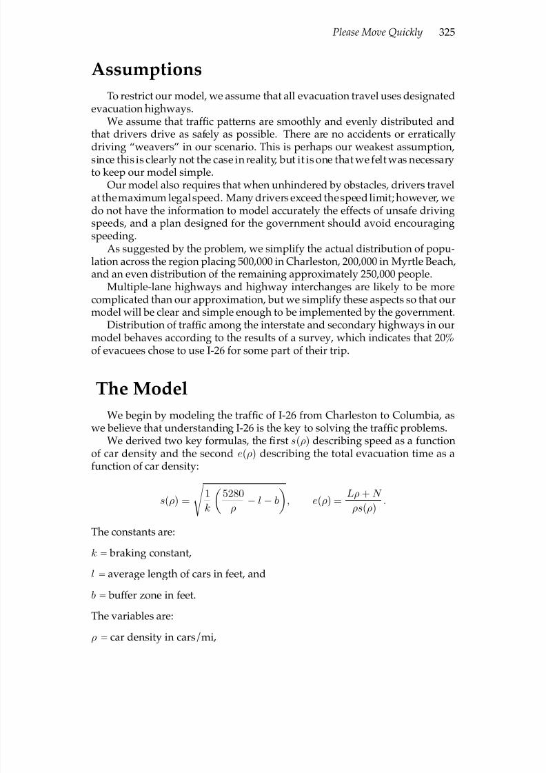
7/17/2019 UMAP 2001 vol. 22 No. 3



Assumptions

To restrict our model, we assume that all evacuation travel uses designatedevacuation highways.

We assume that traf Þc patterns are smoothly and evenly distributed and

that drivers drive as safely as possible. There are no accidents or erraticallydriving “weavers” in our scenario. This is perhaps our weakest assumption,since this is clearly not the case in reality, but it is one that we felt was necessaryto keep our model simple.

Our model also requires that when unhindered by obstacles, drivers travelat themaximum legalspeed. Many drivers exceed thespeedlimit; however, wedo not have the information to model accurately the effects of unsafe drivingspeeds, and a plan designed for the government should avoid encouragingspeeding.

As suggested by the problem, we simplify the actual distribution of popu-lation across the region placing 500,000 in Charleston, 200,000 in Myrtle Beach,

and an even distribution of the remaining approximately 250,000 people.Multiple-lane highways and highway interchanges are likely to be more

complicated than our approximation, but we simplify these aspects so that ourmodel will be clear and simple enough to be implemented by the government.

Distribution of traf Þc among the interstate and secondary highways in ourmodel behaves according to the results of a survey, which indicates that 20%of evacuees chose to use I-26 for some part of their trip.

The Model

We begin by modeling the traf Þc of I-26 from Charleston to Columbia, aswe believe that understanding I-26 is the key to solving the traf Þc problems.

We derived two key formulas, the Þrst s(ρ) describing speed as a functionof car density and the second e(ρ) describing the total evacuation time as afunction of car density:

s(ρ) =

1

k

5280

ρ − l − b

, e(ρ) =

Lρ + N

ρs(ρ) .

The constants are:

k = braking constant,

l = average length of cars in feet, and

b = buffer zone in feet.

The variables are:

ρ = car density in cars/mi,

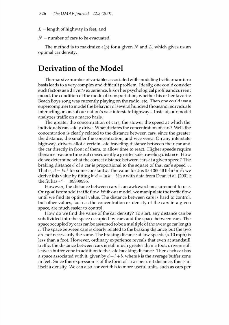
7/17/2019 UMAP 2001 vol. 22 No. 3



L = length of highway in feet, and

N = number of cars to be evacuated.

The method is to maximize e(ρ) for a given N and L , which gives us anoptimal car density.

Derivation of the Model

Themassive number of variablesassociatedwith modelingtraf Þconamicro basis leads to a very complex and dif Þcult problem. Ideally, one could considersuch factors asa driver’sexperience, hisorher psychological proÞleandcurrentmood, the condition of the mode of transportation, whether his or her favoriteBeach Boys song was currently playing on the radio, etc. Then one could use asupercomputer to model thebehavior of several hundred thousand individuals

interacting on one of our nation’s vast interstate highways. Instead, our modelanalyzes traf Þc on a macro basis.The greater the concentration of cars, the slower the speed at which the

individuals can safely drive. What dictates the concentration of cars? Well, theconcentration is clearly related to the distance between cars, since the greaterthe distance, the smaller the concentration, and vice versa. On any interstatehighway, drivers allot a certain safe traveling distance between their car andthe car directly in front of them, to allow time to react. Higher speeds requirethe same reaction time but consequently a greater safe traveling distance. Howdo we determine what the correct distance between cars at a given speed? The braking distance d of a car is proportional to the square of that car’s speed v.

That is, d = kv2 for some constant k. The value for k is 0.0136049 ft-hr2mi2; wederive this value by Þtting ln d = ln k + b ln v with data from Dean et al. [2001];the Þt has r2 = .99999996.

However, the distance between cars is an awkward measurement to use.Ourgoalistomodeltraf Þcßow. With ourmodel,we manipulate thetraf Þcßowuntil we Þnd its optimal value. The distance between cars is hard to control, but other values, such as the concentration or density of the cars in a givenspace, are much easier to control.

How do we Þnd the value of the car density? To start, any distance can besubdivided into the space occupied by cars and the space between cars. Thespaceoccupiedbycarscan beassumed to bea multipleof the average car lengthl. The space between cars is clearly related to the braking distance, but the twoare not necessarily the same. The braking distance at low speeds (< 10 mph) isless than a foot. However, ordinary experience reveals that even at standstilltraf Þc, the distance between cars is still much greater than a foot; drivers stillleave a buffer zone in addition to the safe breaking distance. Then each car hasa space associated with it, given by d + l + b , where b is the average buffer zonein feet. Since this expression is of the form of 1 car per unit distance, this is initself a density. We can also convert this to more useful units, such as cars per

7/17/2019 UMAP 2001 vol. 22 No. 3



mile:

ρ = cars

mi =

cars

ft × 5280 ft

mi =

5280

d + b + l × cars

mi =

5280

kv2 + b + l

cars

mi .

Solving for v gives

s(ρ) = v =

1

k

5280

ρ − l − b

.

At this point we can substitute k = 0.0136049 ft · h2/mi2 , l = 17 ft (fromresearching sizes of cars), and b = 10 ft (from our personal experience) andgraph speed as a function of density (Figure 1).

Figure 1. Speed as a function of density.

Note the maximum density at 195.6 cars/mi. To understand why a maxi-mum density exists, consider the case b = 0; as v → 0 , the distance between thecars approaches zero.

We now determine how long it takes this group of cars to reach their desti-nation. For now, we say that the group reaches its goal whenever the Þrst cararrives. This is a simple calculation: We divide the length of the road L by theaverage speed of the group

t(ρ) = L

s(ρ) =

L 1

k

5280

ρ − l − b

.

7/17/2019 UMAP 2001 vol. 22 No. 3



Figure 2. Evacuation time as a function of density.

We refer to this function as t because it gives the time of the trip. Figure 2 givest for I-26 between Charleston and Columbia, which has a length of 117 mi.

However, the real problem is not simply evacuating one group of cars, itis quickly evacuating a large number of cars. Our goal poses an interestingdilemma: If we evacuate in a stream of low density, they will travel very fast

but evacuation takes an extremely long time. If we evacuate in a stream of veryhigh car density (which is what happened during Hurricane Floyd), manypeople will move at once but they will move very slowly. We must seek themiddle ground.

We express the total evacuation time as a function of car density; then takingthe minimum gives the optimum car density.

Unfortunately, the concept of average car density doesn’t work as well overlarge distances. The problem with traf Þc ßow is that it tends to clump, creatinghigh cardensitiesandthus lowspeeds. However, theinstantaneous cardensitywon’t vary much for a small distance, such as a mile, compared to the averagecar density over the entire highway. To look ahead to the problem: Making

I-26 one-way will certainly help facilitate evacuation, but it won’t help nearlyas much as staggering the evacuation ßow. Staggering is the only way torealistically create a constant traf Þc ßow and thus an average car density thatis more or less constant over the entire length of the highway.

Suppose that we take the N cars that need to be evacuated and subdividethem into groups, each consisting of the number of cars that there are in 1 mi.Call these groups packets. Each packet is 1 mi long.

We look at two cases, one where we send only one group and another where

7/17/2019 UMAP 2001 vol. 22 No. 3



we send more than one group. For the Þrst case, we assume that all N carsÞt in one packet, so 0 < N < 196 , where 196 is the maximum car density forour values of buffer zone and average car length. Everyone is not technicallyevacuated until the end of the packet arrives safely, so we need to add to t(ρ)the additional time for the end of the packet to arrive:

e(ρ) = t(ρ) + 1

s(ρ).

We call this expression e because it express total evacuation time as a functionof car density.

For the second case, we can say that the packets travel like a train, as youcan’t release another packet until the Þrst packet is a mile away. Evacuationtime is the sum of the time for the Þrst packet to arrive plus the time until thelast packet arrives. Since the packets arrive in order, and they are all one milelong, the time it takes the last packet to arrive is equal to the number of packets

times the time it takes the packets to move 1 mi. The equation is

e(ρ) = t(ρ) + 1

s(ρ)

N

ρ .

For one packet, this second equation simpliÞes to the Þrst.After some algebra, we arrive at

e(ρ) = Lρ + N

ρs(ρ) .

The total evacuation time e is simply a function of three variables: the length

of the highway L , the number of cars N , and the car density ρ. The speed s(ρ)is itself a function of ρ and three other constants (the braking constant k , theaverage car length l , and the buffer zone b). Setting L = 117 and N = 65,000produces the graph in Figure 3 , which has a clear minimum.

Application of the Model

The model shouldÞrstdeal with I-26. We assume that evacuation along thisroad takes the longest. We limit our consideration to Charleston, Columbia,

and I-26 between them.

Modeling I-26 TrafÞc Flow

The problem states that the evacuation consists of 500,000 residents fromCharleston, 200,000 from Myrtle Beach, and 250,000 others. However, themodel need not evacuate all 950,000. The evacuation rate of 64% for Hurri-cane Floyd was one of the highest evacuation rates ever seen for a hurricane.

7/17/2019 UMAP 2001 vol. 22 No. 3



Figure 3. Total evacuation time as a function of density.

Many individuals, whether elderly, Þnancially unable to make the trip, or justdarnstubbornremainclosetohomeratherthanjointhethrongoffranticdriversßeeing for their lives. Further, only about 20% of those who left did so alongInterstate 26. Taking 20% of 64% of 950,000 gives 122,000 as the number of people that we can expect to evacuate on I-26.

We must convert number of people to cars, the unit in our model. In SouthCarolina there are 3,716,645 people and 1,604,000 households, or 2.3 people perhousehold. Further research allowed us to Þnd the average number of carstaken for each household. Dow and Cutter [2001] included Table 2 on thenumber cars taken by each household.

Table 2.

Cars taken by each household in 1999 Hurricane Floyd evacuation [Dow and Cutter 2001].

Cars % of households

0 3%

1 72%2 21%3+ 4%

Since the number of households taking more than three cars is merely afraction of the 4% of the population evacuating, we assume that a householdtakes0,1,2,or3cars. Thus,weÞnd a weightedaverage of 1.26 cars/household.

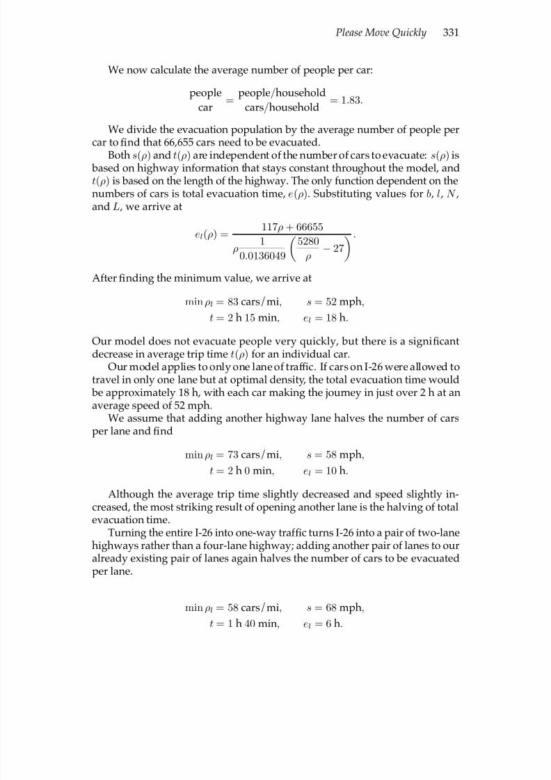
7/17/2019 UMAP 2001 vol. 22 No. 3



We now calculate the average number of people per car:

people

car =

people/household

cars/household = 1.83.

We divide the evacuation population by the average number of people percar to Þnd that 66,655 cars need to be evacuated.

Both s(ρ) and t(ρ) are independent of the number of cars to evacuate: s(ρ) is based on highway information that stays constant throughout the model, andt(ρ) is based on the length of the highway. The only function dependent on thenumbers of cars is total evacuation time, e(ρ). Substituting values for b , l , N ,and L , we arrive at

el(ρ) = 117ρ + 66655

ρ 1

0.0136049

5280

ρ − 27

.

After Þnding the minimum value, we arrive at

min ρl = 83 cars/mi, s = 52 mph,

t = 2 h 15 min, el = 18 h.

Our model does not evacuate people very quickly, but there is a signiÞcantdecrease in average trip time t(ρ) for an individual car.

Our model applies to only one lane of traf Þc. If cars on I-26 were allowed totravel in only one lane but at optimal density, the total evacuation time would be approximately 18 h, with each car making the journey in just over 2 h at an

average speed of 52 mph.We assume that adding another highway lane halves the number of carsper lane and Þnd


t = 2 h 0 min, el = 10 h.

Although the average trip time slightly decreased and speed slightly in-creased, the most striking result of opening another lane is the halving of totalevacuation time.

Turning the entire I-26 into one-way traf Þc turns I-26 into a pair of two-lane

highways rather than a four-lane highway; adding another pair of lanes to ouralready existing pair of lanes again halves the number of cars to be evacuatedper lane.


t = 1 h 40 min, el = 6 h.

7/17/2019 UMAP 2001 vol. 22 No. 3



Conclusions from the I-26 Model

The problem explicitly mentions four means by which traf Þc ßow may beimproved:

• turning I-26 one-way,• staggering evacuation,

• turning smaller highways one-way, or

• limiting the number or type of cars.

Staggering

Contrary to the emphasis of the South Carolina Emergency PreparednessDivision (SCEPD), the primary proposal should not be the reversal of south- bound traf Þc on I-26 but rather the establishment of a staggering plan. Oneglance at the total evacuation time vs. car density graph reveals the great bene-Þts gained from maintaining a constant and moderate car density on the high-way. The majority of the problems encountered during Hurricane Floyd, suchas the 18-hour trips to Columbia or incidents of cars running out of gas on thehighway, would be solved if a constant car density existed on the highway.

However, while our model assumes a certain constant car density, it doesnotprovide a methodforproducing such density. Therefore, theSCEPDshouldproduce a plan that staggers the evacuation to maintain a more constant cardensity. One proposal was a county-by-county stagger. SCEPD should take

the optimal car density and multiply that by the optimal speed to arrive at anoptimal value of cars/hour. The SCEPD should then arrange the stagger sothat dispersal of cars per hour is as close as possible close to the optimal value.

Making I-26 One-Way

In addition to the staggering plan, making I-26 one-way reduces the totalevacuation time from 10 h to 6 h. Thus, while staggering should always beimplemented, reversal of traf Þc on I-26 should supplement the staggering planwhen the SCEPD desires a shorter evacuation time.

The Other Options

This leaves two more strategies for managing traf Þc ßow: turning smallerhighways one-way and limiting the number or types of car taken per house-hold. Both of these can be implemented easily in our model. Turning smallerhighways one-way would encourage evacuees to take back roads instead of I-26, making percentage of evacuees taking I-26 less than 20%, reducing our

7/17/2019 UMAP 2001 vol. 22 No. 3



value for N . Restricting the number of cars per household would also reduceN . Likewise, disallowing large vehicles would reduce l , the average length of vehicles.

Considering that the optimal speed calculated after making I-26 one-way is68 mph, and that adding other evacuation strategies would raise the optimum

average speed above the lawful limit of 70 mph, additional strategies would be unnecessary.

Adding Myrtle Beach

Thenext routeneeding consideration is 501/I-20 leaving MyrtleBeach,with200,000 people. Unfortunately, we lack statistics on how many people took the501/I-20 evacuation route. We can, however, make a guess using a ratio. Weassume that an equal proportion of residents of Myrtle Beach evacuate usingthe main route as in Charleston, so that the number taking the highway leaving

a city is directly proportional to the city’s size. This suggests that 49,000 peopleleave MyrtleBeach in 49,000/1.84 = 26,600cars, or13,300cars/lane. Combiningthis with an L = 150 mi, the distance between Myrtle Beach and Columbia, wecan apply our model to arrive at


t = 1 h 50 min, el = 5 h 28 min.

Wecapthespeedat70mphanddetermineapreferredcardensityof56cars/mi.This Þgure produces a new set of optimal values:


t = 2 h, el = 5 h 30 min.

This calculation also conÞrms one of our basic assumptions, that I-26 betweenCharleston and Columbia is the limiting factor: Evacuation from Myrtle Beachusing two lanes still takes less time (5 h) than evacuation using 4 lanes on I-26from Charleston (6 h). From this we can conclude that making traf Þc roadsleading from Myrtle Beach one-way would be unnecessary. We assume thatapplying our model to other smaller highways will lead to similar results.

Adding Intersections and I-95To simplify the model, we assume that intersecting routes of equal density

contribute traf Þc to the adjoining route so that the difference in densities alwaysseeks a balance. Intersections between roads of similar relative density do notcause unexpected spikes in density on either road. Their effect is thereforenegligible.

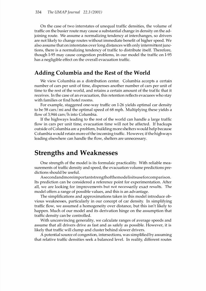
7/17/2019 UMAP 2001 vol. 22 No. 3



On the case of two interstates of unequal traf Þc densities, the volume of traf Þc on the busier route may cause a substantial change in density on the adjoining route. We assume a normalizing tendency at interchanges, so driversare not likely to change routes without immediate beneÞt of higher speed. Wealso assume that on interstates over long distances with only intermittent junc-

tions, there is a normalizing tendency of traf Þc to distribute itself. Therefore,though I-95 may cause congestion problems, in our model the traf Þc on I-95has a negligible effect on the overall evacuation traf Þc.

Adding Columbia and the Rest of the World

We view Columbia as a distribution center. Columbia accepts a certainnumber of cars per unit of time, dispenses another number of cars per unit of time to the rest of the world, and retains a certain amount of the traf Þc that itreceives. In the case of an evacuation, this retention reßects evacuees who stay

with families or Þ

nd hotel rooms.For example, staggered one-way traf Þc on I-26 yields optimal car densityto be 58 cars/mi and the optimal speed of 68 mph. Multiplying these yields aßow of 3,944 cars/h into Columbia.

If the highways leading to the rest of the world can handle a large traf Þcßow in cars per unit time, evacuation time will not be affected. If backupsoutside of Columbia are a problem, building more shelters would help becauseColumbia would retain more of the incoming traf Þc. However, if the highwaysleading elsewhere can handle the ßow, shelters are unnecessary.

Strengths and WeaknessesOne strength of the model is its formulaic practicality. With reliable mea-

surements of traf Þc density and speed, the evacuation volume predictions pre-dictions should be useful.

Asecondandmoreimportantstrengthofthemodelisitsuseforcomparison.Its prediction can be considered a reference point for experimentation. Afterall, we are looking for improvements but not necessarily exact results. Themodel offers a range of possible values, and this is an advantage.

The simpliÞcations and approximations taken in this model introduce ob-vious weaknesses, particularly in our concept of car density. In simplifyingtraf Þc ßow, we assumed a homogeneity over distance, but this isn’t likely tohappen. Much of our model and its derivation hinge on the assumption thattraf Þc density can be controlled.

With unconvincing generality, we calculate ranges of average speeds andassume that all drivers drive as fast and as safely as possible. However, it islikely that traf Þc will clump and cluster behind slower drivers.

A potential source of congestion, intersections, was simpliÞed by assumingthat relative traf Þc densities seek a balanced level. In reality, different routes

7/17/2019 UMAP 2001 vol. 22 No. 3



are preferred over others and imbalances in traf Þc density are likely to occur.The only way to test the model is to collect data during very heavy traf Þc.

However, traf Þc as great as during Hurricane Floyd is rare.In short, the weaknesses of the model are primarily related to its simplicity.

However, it is that same simplicity that is its greatest strength.

References

Cutter, Susan L., Kirsten Dow, Robert Oldendick, and Patrice Burns. SouthCarolina’s EvacuationExperience withHurricaneFloyd. http://www.cla.sc.edu/geog/hrl/Floyd_evac.html . Accessed February 10, 2001.

Dean, Ryan, Drew Morgan, and David Ward. Braking distance of a movingcar. http://199.88.16.12/~team99b/tech.html . Accessed February 10,2001.

Dow, Kirsten, and Susan L. Cutter. South Carolina’s Response to HurricaneFloyd. http://www.colorado.edu/hazards/qr/qr128/qr128.html . Ac-cessed February 10, 2001.

Locke, John. [1690]. Second Treatise On Government. http://www.swan.ac.uk/poli/texts/locke/lockcont.htm . Accessed February 12, 2001.

Weiss, Neil, and Matthew Hassett. 1982. Introductory Statistics. Reading, MA:Addison-Wesley.

Dr. Ann Watkins, President of the Mathematical Association of America, congratulating MAAWinner Adam Dickey after he presented the team’s model at MathFest in Madison, WI, in August.[Photo courtesy of Ruth Favro.]

7/17/2019 UMAP 2001 vol. 22 No. 3



Mathematical Commission Stream-lines Hurricane Evacuation Plan

Columbia, SC, Feb. 12— As long as

the western coast of Africa stays where itis, global climate patterns will continue tohave it in for South Carolina. That prover-

bial “it” is the hurricane season. Somemay point their Þngers at God and curseHis ways, but cooler heads will eventuallysurrender—shutter their windows, pack their cars, and drive to Columbia for thenext few days, mood unsettled.

However, a report issuedfrom thegov-ernor’s of Þce earlier this week announcedthat scientists have designed a new plan

for coastal emergency evacuation.Prompted by public disapproval of

evacuation tactics used during the manda-tory evacuation ordered during HurricaneFloyd, the new study sought to Þnd thesource of the congestion problems thatleft motorists stranded on I-26 for up to18 hours wondering why they even at-tempted evacuation at all.

“The government should have knownthat we didn’t have the roads to get every-

body out,” one Charleston resident com-mented, “and we just had the speed limitsraised, so I would’ve expected a quickerescape rout.”

Governor Jim Hodges commissionedthe evacuationstudy last Friday, expectinga quick response. So far, the results seemplausible and practical.

The private commission developed amathematical model to describe the traf-Þc ßow that caused the backups respon-sible for the evacuation problems. Then,

by manipulating the model and combiningit with statistical survey data collected af-ter the evacuation, the commission devel-oped a report evaluating the various cur-rent suggestions to alleviate issues.

The Þndings of the commission sug-

gest that the best way to avoid evacua-

tion backups is to stagger and sequencethe county and metropolitan evacuationorders so that main routes do not exceedthe critical traf Þc density that caused theslowdown.

As explained by one member of thecommission, “the model does not get intothe gritty details of complicated traf Þcmodeling, but it does present a usefulframework for evaluating crisis plans andtraf Þc routing.”

The solution garnered some skeptical

criticism among mathematics researchersstate-wide. “The commission is missingthepoint here,”commentedoneresearcherat the Hazards Research Lab in the De-partment of Geology at the University of South Carolina. “The problem with Hur-ricane Floyd wasan anomalously high rateof evacuation among coastal residents—this is a sociopsychological problem andnot a mathematical one.”

Despite the cool reception, the com-

mission is conÞ

dent in its Þ

ndings. Ac-cording to the report, a general stagger-ing of traf Þc will far exceed the beneÞts of other methods of congestion control thathave been suggested, such as reversingthe eastbound lanes of I-26 and some sec-ondary highways.

“We Þnd that advance planning with amind to reduce the traf Þc surge associatedwith quickly ordered mandatory evacua-tions is the most useful way to improveevacuations,” said a spokesman for the

commission.Despite the current concerns, the prov-

inggroundsforthe Þndingsofthecommis-sion will not surface until this fall, whenthe tropical swells off the coast of Africa

begin heading our way again.

—Corey R. Houmand, Andrew D. Pruett, and Adam S. Dickey in Winston–Salem, NC.

7/17/2019 UMAP 2001 vol. 22 No. 3


Judge’s Commentary 337

Judge’s Commentary:

The Outstanding Hurricane

Evacuation PapersMark ParkerDepartment of Mathematics, Engineering, and Computer ScienceCarroll CollegeHelena, MT 59625 [email protected]

http://web.carroll.edu/mparker

Introduction

Once again, Problem B proved to be quite challenging—both for the stu-dent teams and for the judges! The students were challenged by a multifacetedproblem with several dif Þcult questions posed, andthe judgeswere challengedto sort through the wide range of approaches to Þnd a small collection of the best papers. It is worth reminding participants and advisors that Outstand-ing papers are not without weaknesses and even mathematical or modelingerrors. It is the nature of judging such a competition that we must trade off thestrengths, both technical and expository, of a given paper with its weaknesses,

and make comparisons between papers the same way.The approaches taken by this year’s teams can be divided into two general

categories:

Macroscopic: Traf Þc on a particular highway or segment of highway was con-sidered to be a stream, and a ßow rate for the stream was characterized.Among the successful approaches in this category were ßuid dynamics andnetwork ßow algorithms.

Microscopic: These canbe consideredcar-followingmodels, wherethespacing between and the speeds of individual vehicles are used to determine the

ßow. Among the successful approaches were discrete event simulations(including cellular automata) and queuing systems.

TheUMAPJournal22 (3)(2000)337–343. cCopyright2001 by COMAP, Inc. All rightsreserved.Permission to make digital or hard copies of part or all of this work for personal or classroom useis granted without fee provided that copies are not made or distributed for proÞt or commercialadvantage and that copies bear this notice. Abstracting with credit is permitted, but copyrightsfor components of this work owned by others than COMAP must be honored. To copy otherwise,to republish, to post on servers, or to redistribute to lists requires prior permission from COMAP.

7/17/2019 UMAP 2001 vol. 22 No. 3



By far, the most common approach was to determine that the ßow q , or ßux,is a function of the density ρ of cars on a highway and the average speed v of those cars: q = ρv. Successful approaches identiÞed the following characteris-tics of the basic traf Þc ßow problem:

• When the vehicle density on the highway is 0, the ß

ow is also 0.• As density increases, the ßow also increases (up to a point).

• When the density reaches its maximum, or jam density ρ0 , theßow must be 0.

• Therefore, the ßow initially increases, as density does, until it reaches somemaximum value. Further increase in the density, up to the jam density,results in a reduction of the ßow.

At this point, many teams either derived fromÞrst principles or used one of themany resources available on traf Þc modeling (such as Garber and Hoel [1999])

to Þ

nd a relationship between the density and the average speed. Three of thecommon macroscopic models were:

• a linear model developed by Greenshield:

v = v0

1− ρ

ρ0

, so q = ρv0

1− ρ

ρ0

;

• a ßuid-ßow model developed by Greenberg:

v = v0 log ρ

ρ0, so q = ρv0 log

ρ

ρ0;

or

• a higher-order model developed by Jayakrishnan:

v = v0

1− ρ

ρ0

a, so q = ρv0

1− ρ

ρ0

a,

where v0 represents the speed that a vehicle would travel in the absence of other traf Þc (the speed limit). By taking the derivative of the ßow equationwith respect to speed (or density), teams then found the optimal speed (ordensity) to maximize ßow.

Many teams took the optimal ßow from one of the macroscopic approachesand used it as the basis for a larger model. One of the more common modelswas simulation, to determine evacuation times under a variety of scenarios.

In order to make it beyond the Successful Participant category, teams hadto Þnd a way realistically to regulate traf Þc density to meet these optimalityconditions. Many teams did this by stipulating that ramp metering systems(longterm) orstaggered evacuations(short term) couldbeused to control traf Þcdensity.

7/17/2019 UMAP 2001 vol. 22 No. 3



There were a number of mathematically rigorous papers that started witha partial differential equation, derived one of the macroscopic formulas, de-termined appropriate values for the constants, calculated the density givingthe optimal ßow, and incorporated this ßow value into an algorithm for de-termining evacuation time. In spite of the impressive mathematics, if no plan

was given to regulate traf Þc density, the team missed an important concept of the MCM: the realistic application of a mathematical solution to a real-worldproblem.

One key to successful model building is to adapt existing theory or modelsproperly to the problem at hand, so judges see little difference between deriv-ing these equations from Þrst principles and researching them from a book.Whether derived or researched, it is imperative to demonstrate an understand-ing of the model you are using.

The Judging

No paper completely analyzed all 6 questions, so the judges were intrigued by what aspects of the problem that a team found most important and/orinteresting. We were similarly interested in determining what aspects of theproblem a team found least relevant and how they divided their effort amongthe remaining questions. To be considered Outstanding, a paper had to meetseveral minimum requirements:

• the paper must address all 6 questions,

• all required elements (e.g., the newspaper article) must be included, and

• some sort of validation of the model must be included.

We were also particularly interested in how teams modeled the I-26/I-95 inter-change and the congestion problem in Columbia. Many teams chose to treatColumbiaastheterminalpointoftheirmodelandassumedthatallcarsarrivingthere would be absorbed without creating backups.

To survive the cut between Honorable Mention and Meritorious, a paperhad tohavea uniqueaspecton some portion of the problem. Twoexamples thatcome to mind are a unique modeling approach or some aspect of the problemanalyzed particularly well. Thus, papers that failed to address all questions or

had a fatal weakness that prevented their model from being extended couldstill be considered Meritorious. The Meritorious papers typically had verygood insight into the problem, but deÞciencies as minor as missing parame-ter descriptions or model implementation details prevented them from beingconsidered Outstanding.

7/17/2019 UMAP 2001 vol. 22 No. 3



The Outstanding Papers

The six papers selected as Outstanding were recognized as the best of thesubmissions because they:

• developed a solid model which allowed them to address all six questions,and analyze at least one very thoroughly;

• made a set of clear recommendations;

• analyzed their recommendations within the context of the problem; and

• wrote a clear and coherent paper describing the problem, their model, andtheir recommendations.

Here is a brief summary of the highlights of the Outstanding papers.The Bethel College team used a basic car-following model to determine an

optimal density, which maximized ß

ow, for individual road segments. Theythen formulated a maximum ßow problem, with intersections and cities asvertices and road segments as arcs. The optimal densities were used as arccapacities, the numbers of vehicles to be evacuated from each city were usedas the sources, and cities at least 50 miles inland were deÞned to be sinks. Eachcity was then assigned an optimal evacuation route, and total evacuation timesunder the different scenarios were examined.

The Duke team also used a basic car-following model from the traf Þc-modeling literature. This model providedthe foundation of a one-dimensionalcellular automata simulation. Theydida particularlygood jobof deÞningevac-uation performance measures—maximum traf Þc ßow and minimum transit

time, and analyzing traf Þc mergers and bottlenecks—aspects of the problemignored by many other teams.

What discussion of Outstanding papers would be complete without a Har-vey Mudd team? Of the teams that utilized literature-based models, this teamdid the best job of considering advanced parameters—including road grade,non-ideal drivers, and heavy-vehicle modiÞcation. They also did a very good job of comparing their model with the new South Carolina evacuation plan,recognizing the bottleneck problem in Columbia, and analyzing the impact of extra drivers from Florida and Georgia on I-95. Their entry was a nice exampleof a simple model that was well analyzed and thoroughly explained.

The Virginia Governor’s School team began their analysis by reviewingthe current South Carolina evacuation plan, a baseline to compare their modelagainst. They researched the literature to Þnd traf Þc-ßow equations and thenused a genetic algorithm to assign road orientation and evacuation start timesfor cities. They did an exceptionally good job of analyzing the sensitivity of their model to changes in parameter values.

TheINFORMSprizewinner, fromLawrenceTechnicalUniversity, combinedGreenshield’s modelwitha discreteevent simulation. Thejudges sawthisentryas a solid paper with logical explanations and a good analysis. The team’s

7/17/2019 UMAP 2001 vol. 22 No. 3



model handled bottlenecks, and the team used a simulation of the actual 1999evacuation to validate their model.

The MAA and SIAM winner, from Wake Forest University, derived a car-followingmodel fromÞrstprinciples, whichwasthen incorporatedin a cellularautomata type model. Like many of the best approaches, the parameters for

their model came from the 1999 evacuation. They provided a thoughtful, notnecessarily mathematical, analysis of intersections and I-95.

Advice

At the conclusion of our judging weekend, the judges as a whole offeredthe following comments:

Follow the instructions

• Answer all required parts.• Make a precise recommendation.

• Don’t just copy theoriginal problem statement, butprovide us with yourinterpretation.

Readability

• Make it clear in the paper where the answers are.

• Many judges Þnd it helpful to include a table of contents.

• Pictures and graphs can help demonstrate ideas, results, and conclu-sions.

• Use discretion: If your paper is excessively long (we had a paper thisyear that was over 80 pp, not including computer program listing!),you should probably reconsider the relevance of all factors that you arediscussing. Depending on what round of judging your paper is beingread, judges typically have between 5 and 30 minutes to read it.

Computer Programs

• Make sure that all parameters are clearly deÞned and explained.

• When using simulation, you must run enough times to have statistically

signiÞ

cant output. A single run isn’t enough!• Always include pseudocode and/or a clear verbal description.

Reality Check

• Why do you think your model is good? Against what baseline can youcompare/validate it?

• How sensitive is your model to slight changes in the parameters youhave chosen? (sensitivity analysis)

7/17/2019 UMAP 2001 vol. 22 No. 3



• Complete theanalysis circle: Are your recommendations practical in theproblem context?

Before the Þnal judging of the MCM papers, a Þrst (or triage) round of judging is held. During triage judging, each paper is skimmed by two or three

judges, who spend between 5 and 10 minutes each reading the paper. Typically,whenyousendyourpaperofftoCOMAP,youhaveabouta43%chanceofbeingranked higher than Successful Participant. If, however, you survive the triageround, you have about an 80% chance of being ranked higher than SuccessfulParticipant. Head triage judge Paul Boisen offers the following advice to helpyou survive triage.

Triage Judge Tips

• Your summary is a key component of the paper; it needs to be clearand contain results. A long list of techniques can obscure your results;it is better to provide only a quick overview of your approach. TheLawrence Technical University paper is a good example of a clear andconcise summary.

• Your paper needs to be well organized—can a triage judge understandthe signiÞcance of your paper in 6 to 10 minutes?

Triage Judge Pet Peeves

• Tables with columns headed by Greek letters or acronyms that cannot be immediately understood.

• DeÞnitions and notation buried in the middle of paragraphs of text. A

bullet form is easier for the frantic triage judge!• Equations without variables deÞned.

• Elaborate derivations of formulas taken directly from a text. It is better tocite the book and perhaps brießy explain how the formula is derived. Itismost important todemonstrate thatyou knowhow touse the formulasproperly.

Reference

Garber, Nicholas J., and Lester A. Hoel. 1999. Traf Þc and Highway Engineering.PaciÞc Grove, CA: Brooks/Cole Publishing Company.

7/17/2019 UMAP 2001 vol. 22 No. 3



About the Author

Afterreceiving hisB.A. in MathematicsandComputerScience in1984, Mark Parkerspenteight years working as a systems simulation andanalysis engineerin the defense industry. After completing his Ph.D. in Applied Mathematics at

the University of Colorado–Denver in 1995, he taught mathematics and com-puter science at Eastern Oregon University for two years. He then spent threeyears on the faculty at the U.S. Air Force Academy teaching mathematics andoperations research courses. He now shares a teaching position with his wife,Holly Zullo, at Carroll College in Helena, MT, and spends as much time as hecan with his three-year-old daughter Kira.

7/17/2019 UMAP 2001 vol. 22 No. 3


Documents

UMAP 2001 vol. 22 No. 3