Embed Size (px)
Citation preview

Ultra-Sparse Finite-Di�erencing For Arbitrage-FreeVolatility Surfaces From Your Favourite Stochastic
Volatility Model
25th of September 2014
Outline
1 Introduction
2 Which stochastic volatility model?
3 The DHI volatility framework
4 Application examples
5 Spot Shock Sensitivities
6 Normal Extensions
7 The generator
8 Spatial discretisation
9 Continuous-time perfect martingale
10 Finite-di�erencing stencils
11 Boundary Conditions
12 Ensuring continuous-time stability
13 Numerical integation in time
14 Box transition probability translation
15 Cash dividends
16 Conclusion
(VTB Capital) Ultra-Sparse Finite-Di�erencing 25th of September 2014 2 / 151
1 Introduction Implied volatility representations
Implied volatilities have long been managed via parametric formulations.
Parametric volatility formulations are used for various purposes:-
Convenient management of implied volatility surfaces and option books.
Intuition about the shape of the volatility surface.
Parametrization of the response of volatility to spot moves.
Control of skew/smile-adjusted deltas of vanilla options to the typical be-haviour of the market.
(VTB Capital) Ultra-Sparse Finite-Di�erencing 25th of September 2014 3 / 151
1 Introduction Parametric volatility types Parametric local volatility models
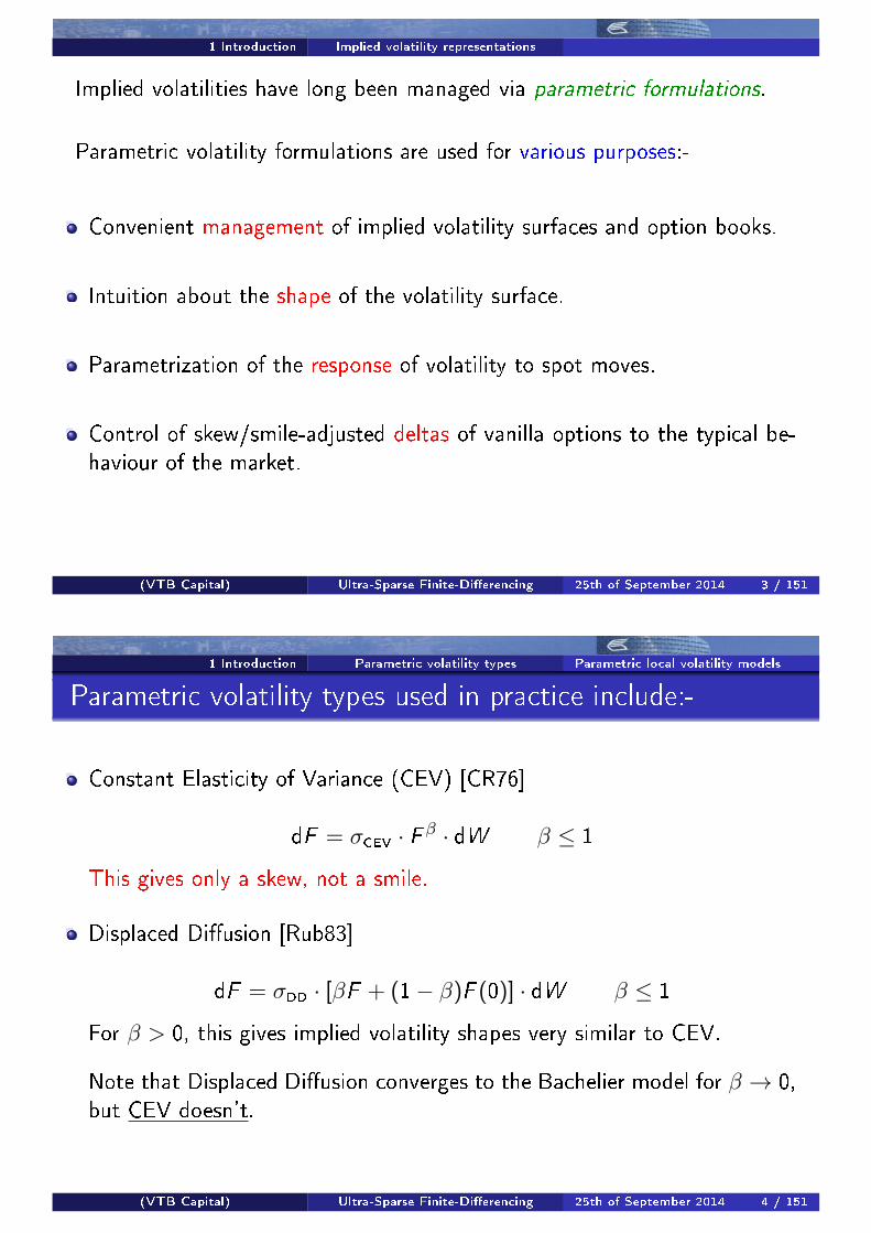
Parametric volatility types used in practice include:-
Constant Elasticity of Variance (CEV) [CR76]
dF = σCEV · F β · dW β ≤ 1
This gives only a skew, not a smile.
Displaced Di�usion [Rub83]
dF = σDD · [βF + (1− β)F (0)] · dW β ≤ 1
For β > 0, this gives implied volatility shapes very similar to CEV.
Note that Displaced Di�usion converges to the Bachelier model for β → 0,but CEV doesn't.
(VTB Capital) Ultra-Sparse Finite-Di�erencing 25th of September 2014 4 / 151
1 Introduction Parametric volatility types Practitioner's pricing practices
Mixture of log-normals
v(F ,K ,T ) = w · B(F ,K , σ1,T ) + (1− w) · B(F ,K , σ2,T )
This is a very old practitioner trick. If you cannot be sure about thevolatility, take the average of (Black prices from) your two best guesses.
This gives only a smile with no skew at the money.
It can be extended to include a skew by allowing for two di�erent forwardsF1 and F2 subject to
w1F1 + w2F2 = F .
Aka �Log-normal mixture dynamics� when mapped via Gyöngyi's theorem
σ2e�ective local volatility(K ) = E[σ(F )2
∣∣F = K]
to a continuous-time (Dupire-style) local volatility model.
(VTB Capital) Ultra-Sparse Finite-Di�erencing 25th of September 2014 5 / 151
1 Introduction Parametric volatility types Stochastic volatility models
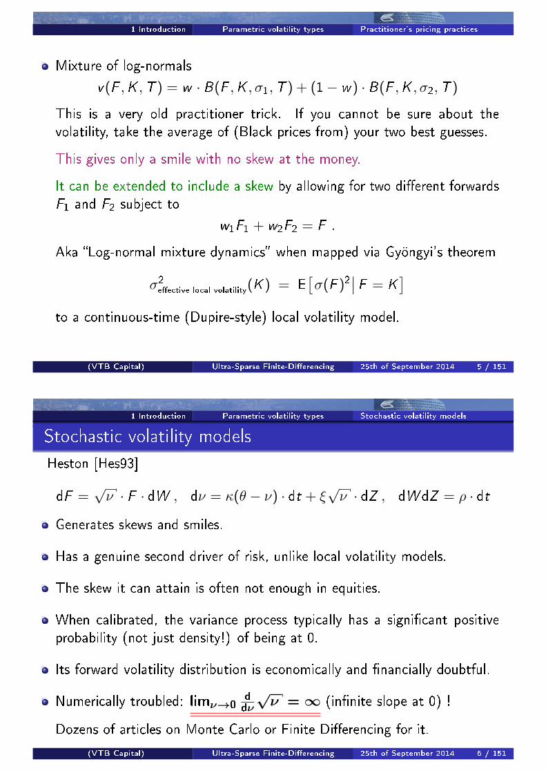
Stochastic volatility models
Heston [Hes93]
dF =√ν · F · dW , dν = κ(θ − ν) · dt + ξ
√ν · dZ , dW dZ = ρ · dt
Generates skews and smiles.
Has a genuine second driver of risk, unlike local volatility models.
The skew it can attain is often not enough in equities.
When calibrated, the variance process typically has a signi�cant positiveprobability (not just density!) of being at 0.
Its forward volatility distribution is economically and �nancially doubtful.
Numerically troubled: limν→0d
dν
√ν =∞ (in�nite slope at 0) !
Dozens of articles on Monte Carlo or Finite Di�erencing for it.
(VTB Capital) Ultra-Sparse Finite-Di�erencing 25th of September 2014 6 / 151
1 Introduction Parametric volatility types Stochastic volatility models
Schöbel-Zhu-Stein-Stein [SZ99, SS91]
dF = σ · F · dW , dσ = κ(θ − σ) · dt + ξ · dZ , dW dZ = ρ · dt
Normal volatility process with mean reversion.
Vanilla options via characteristic functions, as in Heston,but without the analytical trap of the multi-valued logarithm.
Numerically tractable.
Good smiles and skews, but usually not enough for some equity markets.
There is no lump of probability for volatility to be at zero, but there ispositive density (and a lot of it).
A good model, superior to Heston. Sadly much less commonly known.
If only it had a local volatility component...
(VTB Capital) Ultra-Sparse Finite-Di�erencing 25th of September 2014 7 / 151
1 Introduction Parametric volatility types Stochastic volatility models
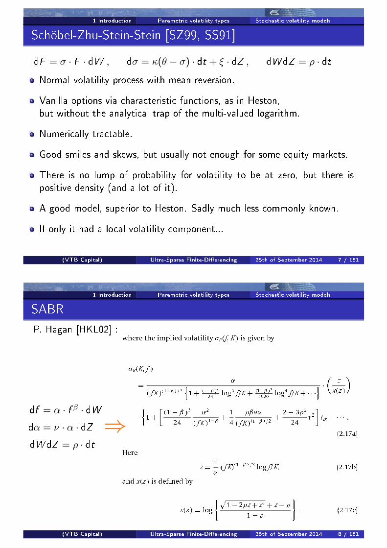
SABR
P. Hagan [HKL02] :
df = α · f β · dWdα = ν · α · dZdW dZ = ρ · dt
⇒
(VTB Capital) Ultra-Sparse Finite-Di�erencing 25th of September 2014 8 / 151
1 Introduction Parametric volatility types Stochastic volatility models
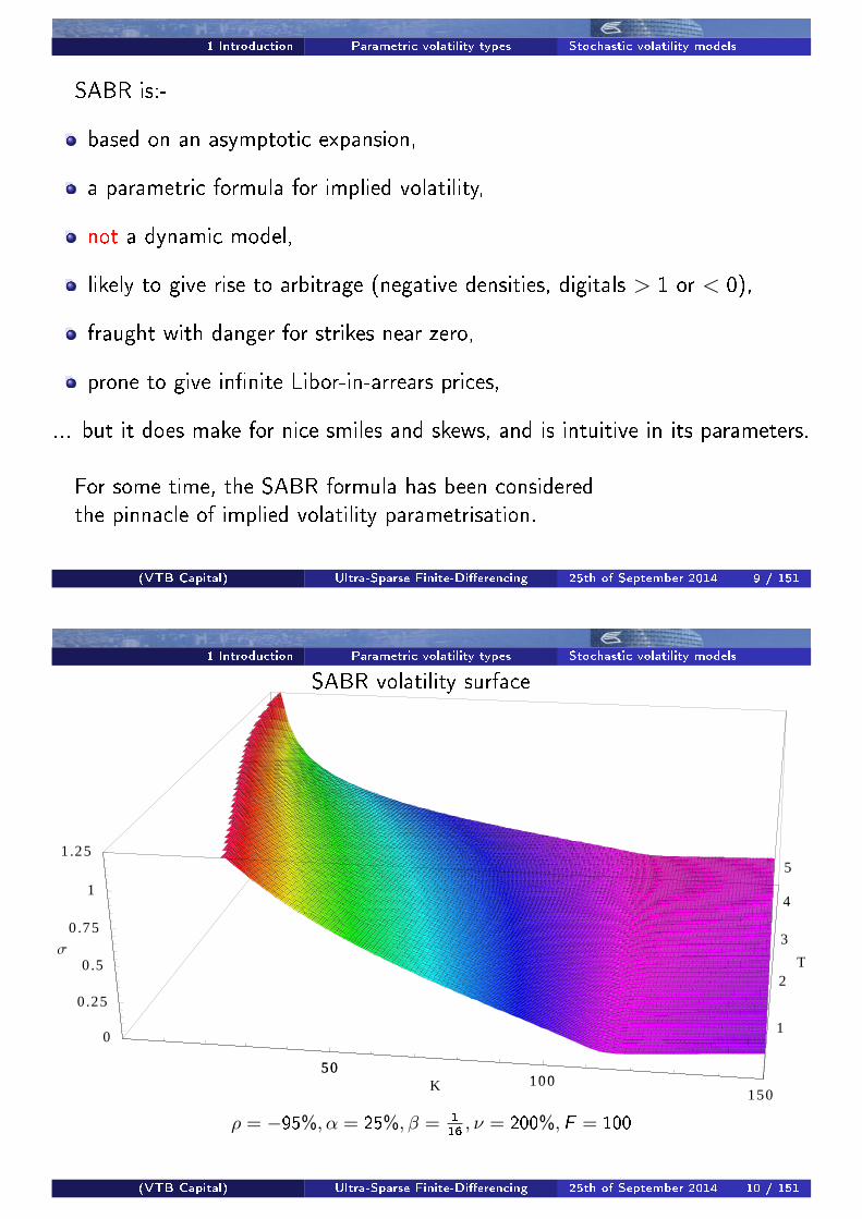
SABR is:-
based on an asymptotic expansion,
a parametric formula for implied volatility,
not a dynamic model,
likely to give rise to arbitrage (negative densities, digitals > 1 or < 0),
fraught with danger for strikes near zero,
prone to give in�nite Libor-in-arrears prices,
... but it does make for nice smiles and skews, and is intuitive in its parameters.
For some time, the SABR formula has been consideredthe pinnacle of implied volatility parametrisation.
(VTB Capital) Ultra-Sparse Finite-Di�erencing 25th of September 2014 9 / 151
1 Introduction Parametric volatility types Stochastic volatility models
50100
150K
1
2
3
4
5
T
0
0.25
0 .5
0 .75
1
1 .25
s
50100
ρ=−95% ,α=200% ,β=1 16 ,F=100
SABR volatility surface
ρ = −95%, α = 25%, β = 116, ν = 200%,F = 100
(VTB Capital) Ultra-Sparse Finite-Di�erencing 25th of September 2014 10 / 151
1 Introduction Parametric volatility types Stochastic volatility models
ρ=−95% ,α=200% ,β=1 16 ,F=100
- 4- 2 0 2
ln HKL
ê
ln H10 L
- 2
- 1
0
ln HT Lê ln H10 L
0
2
4
ln Hs Lê ln H10 L
- 4- 2 0
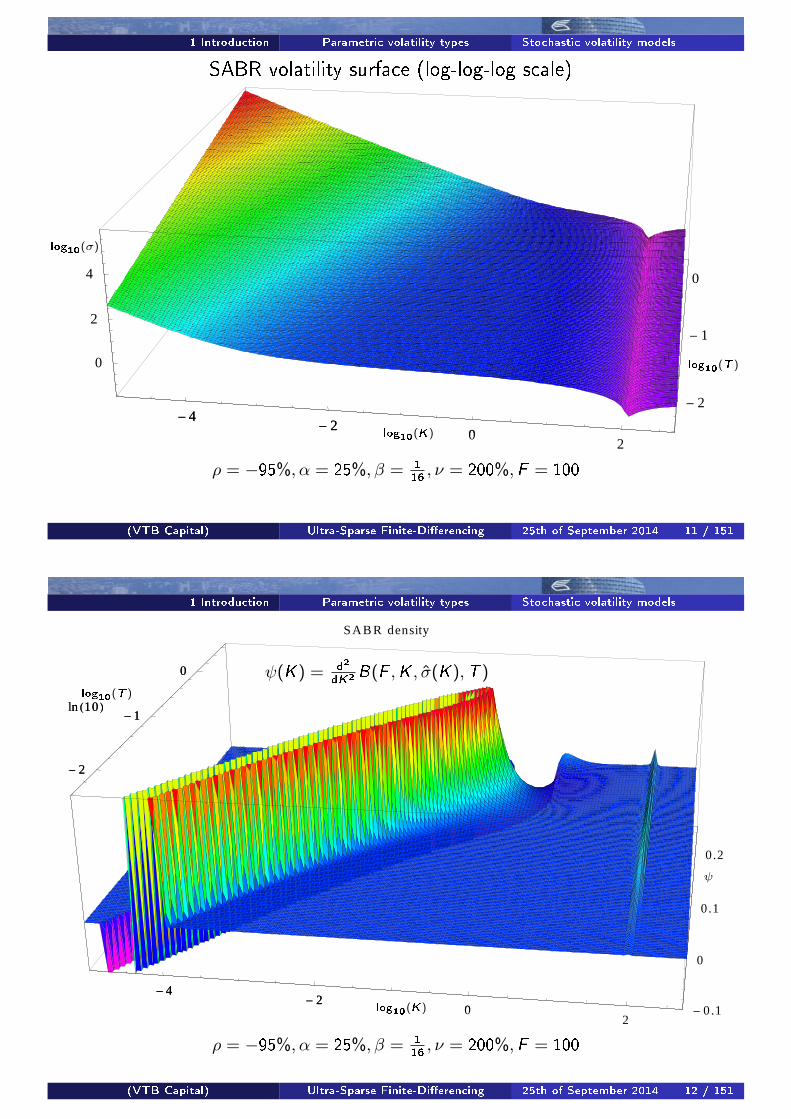
SABR volatility surface (log-log-log scale)
log10(K)
log10(T )
log10(σ)
ρ = −95%, α = 25%, β = 116, ν = 200%,F = 100
(VTB Capital) Ultra-Sparse Finite-Di�erencing 25th of September 2014 11 / 151
1 Introduction Parametric volatility types Stochastic volatility models
ρ=−95% ,α=200% ,β=1 16 ,F=100
SAB R density
- 4- 2
02
ln HKL
ê
ln H10 L
- 2
- 1
0
ln HT Lê ln H10 L
- 0.1
0
0.1
0.2
- 4- 2
0
- 2
- 1
0
lnH
10 L
ψ(K) = d2
dK2B(F ,K , σ̂(K),T )
log10(K)
log10(T )
ψ
ρ = −95%, α = 25%, β = 116, ν = 200%,F = 100
(VTB Capital) Ultra-Sparse Finite-Di�erencing 25th of September 2014 12 / 151
1 Introduction Parametric volatility types Stochastic volatility models
ρ=−95% ,α=200% ,β=1 16 ,F=100
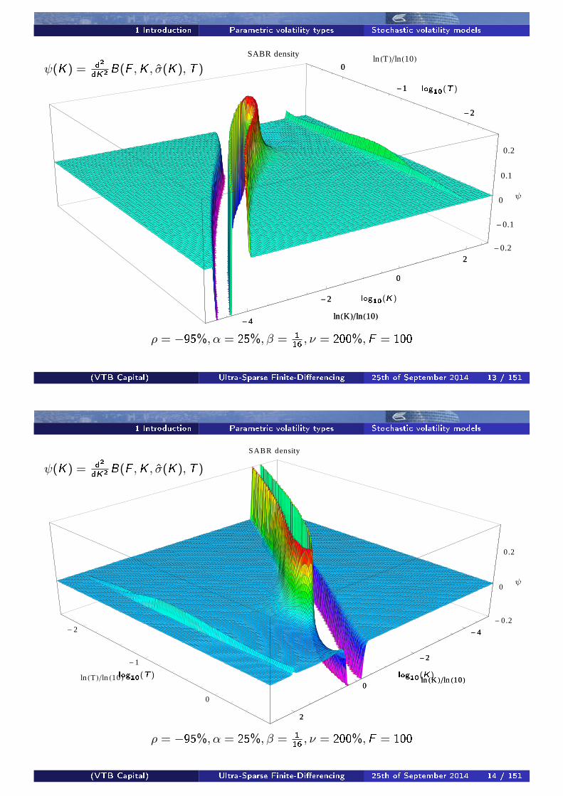
SABR density
-4
-2
0
2
lnHKL
ê
lnH10L
-2
-1
0ln HTL
ê
lnH10 L
-0.2
-0.1
0
0.1
0.2
-4
-2
0
2
lnHKL
ê
lnH10L
-2
-1
0ψ(K) = d2
dK2B(F ,K , σ̂(K),T )
log10(K)
log10(T )
ψ
ρ = −95%, α = 25%, β = 116, ν = 200%,F = 100
(VTB Capital) Ultra-Sparse Finite-Di�erencing 25th of September 2014 13 / 151
1 Introduction Parametric volatility types Stochastic volatility models
ρ=−95% ,α=200% ,β=1 16 ,F=100
SABR density
- 4
- 2
0
2
ln HK Lê ln H10 L
- 2
- 1
0
ln HT Lê ln H10 L
- 0.2
0
0.2
- 4
- 2
0
2
ln HK Lê ln H10 L
ψ(K) = d2
dK2B(F ,K , σ̂(K),T )
log10(K)log10(T )
ψ
ρ = −95%, α = 25%, β = 116, ν = 200%,F = 100
(VTB Capital) Ultra-Sparse Finite-Di�erencing 25th of September 2014 14 / 151

1 Introduction Parametric volatility types Stochastic volatility models
Also, it was noticed that the dynamics of the underlying SDE are unsuitablefor numerical evaluation:
Moment explosions
Singular local volatility slope at F = 0 (when β < 1). The same issue wasthe curse of the Heston model in numerical implementations.
However, and this is very important, SABR does give:-
a dynamic response of the smile to spot movements which enables us tocompute smile-adjusted deltas of vanillas, �Managing Smile Risk� (!),
a sensible volatility surface for constant parameters,
and thus allows for parametric interpolation.
(VTB Capital) Ultra-Sparse Finite-Di�erencing 25th of September 2014 15 / 151
1 Introduction Parametric volatility types Stochastic volatility models
last but not least...
J. Gatheral [Gat04] introduced the Stochastic Volatility Inspired (SVI) form.
It can also create arbitrage.
Its parameters are not as intuitive as SABRs.
It is not quite as �exible as SABR.
It gives no parametric generation of a volatility surface over time.
It gives no parametric response of the volatility surface to spot moves.
It is di�cult to compute smile-adjusted deltas of vanillas.
An alternative formulation for SVI with restricted parameters was publishedin [GJ13]. This, however, is so limited that many �nd it not useful.
(VTB Capital) Ultra-Sparse Finite-Di�erencing 25th of September 2014 16 / 151
1 Introduction Parametric volatility types Stochastic volatility models
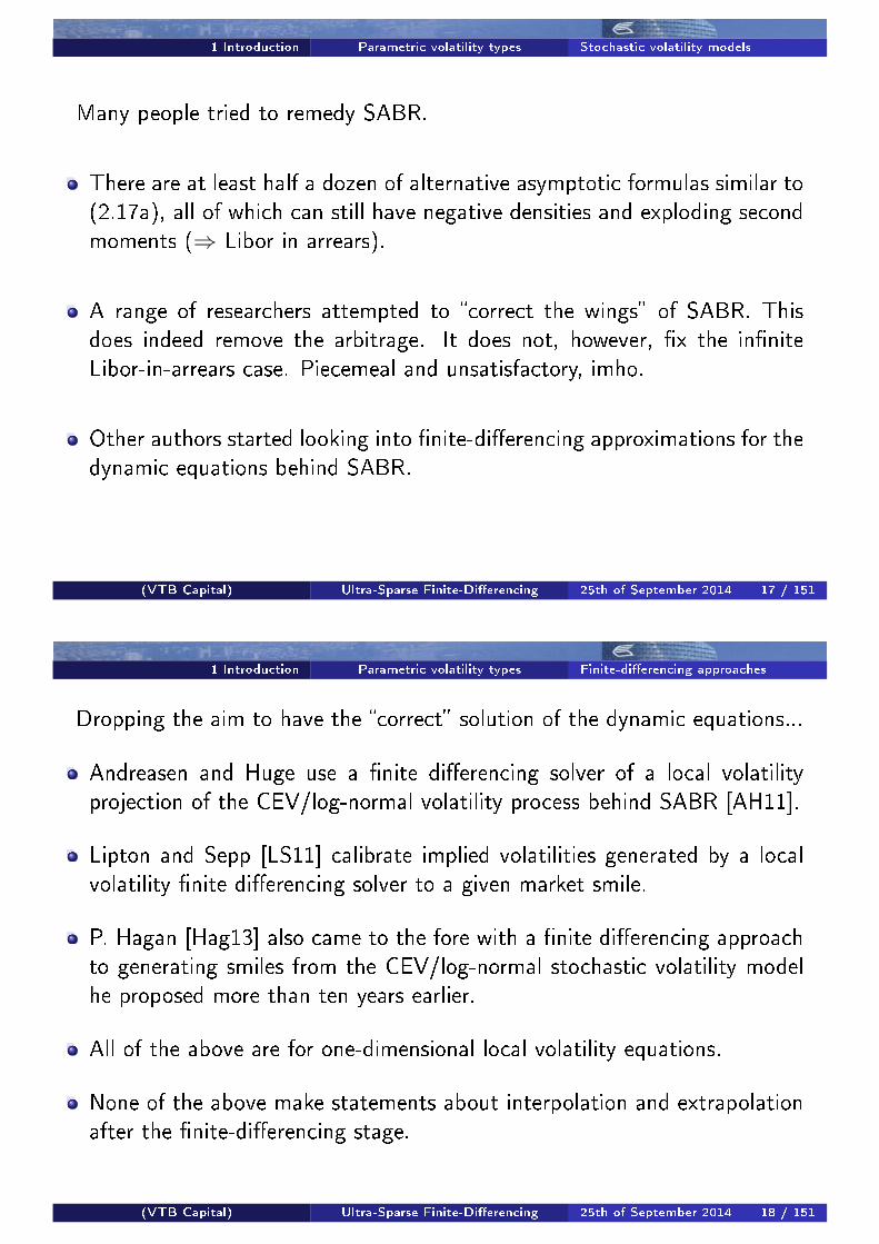
Many people tried to remedy SABR.
There are at least half a dozen of alternative asymptotic formulas similar to(2.17a), all of which can still have negative densities and exploding secondmoments (⇒ Libor in arrears).
A range of researchers attempted to �correct the wings� of SABR. Thisdoes indeed remove the arbitrage. It does not, however, �x the in�niteLibor-in-arrears case. Piecemeal and unsatisfactory, imho.
Other authors started looking into �nite-di�erencing approximations for thedynamic equations behind SABR.
(VTB Capital) Ultra-Sparse Finite-Di�erencing 25th of September 2014 17 / 151
1 Introduction Parametric volatility types Finite-di�erencing approaches
Dropping the aim to have the �correct� solution of the dynamic equations...
Andreasen and Huge use a �nite di�erencing solver of a local volatilityprojection of the CEV/log-normal volatility process behind SABR [AH11].
Lipton and Sepp [LS11] calibrate implied volatilities generated by a localvolatility �nite di�erencing solver to a given market smile.
P. Hagan [Hag13] also came to the fore with a �nite di�erencing approachto generating smiles from the CEV/log-normal stochastic volatility modelhe proposed more than ten years earlier.
All of the above are for one-dimensional local volatility equations.
None of the above make statements about interpolation and extrapolationafter the �nite-di�erencing stage.
(VTB Capital) Ultra-Sparse Finite-Di�erencing 25th of September 2014 18 / 151
2 Which stochastic volatility model? Selection criteria
What do we want?
A. Lipton [2006] :
�The hunt for closed form solutions is ultimately nothingbut the pursuit of fool's gold.�
We don't need to match any idealised continuous process's dynamics.
We need a parametric speci�cation of an implied volatility surface.
We want it to be numerically benign.
We want it to have a consistent response to spot movements
We want it to have explanatory power.
We want to control what vega-adjusted deltas it gives for vanillas.This is equivalent to controlling the ATM volatility response to spot moves.
p. Hagan [Hag13]:�The volatility response should be less than log-linear,
maybe only 80% or so.� More on this later.
(VTB Capital) Ultra-Sparse Finite-Di�erencing 25th of September 2014 19 / 151
2 Which stochastic volatility model? Hyp-Hyp The process equations
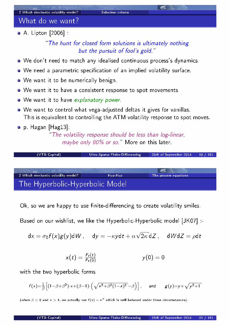
The Hyperbolic-Hyperbolic Model
Ok, so we are happy to use �nite-di�erencing to create volatility smiles.
Based on our wishlist, we like the Hyperbolic-Hyperbolic model [JK07] :-
dx = σ0f (x)g(y)dW , dy = −κydt + α√2κ dZ , dW dZ = ρdt
x(t) = Ft(t)Ft(0) y(0) = 0
with the two hyperbolic forms
f (x)= 1β
[(1−β+β2)·x+(β−1)·
(√x2+β2(1−x)2 −β
)], and g(y)=y+
√y2+1
(when β < 0 and x > 1, we actually use f (x) = xβ which is well behaved under these circumstances).
(VTB Capital) Ultra-Sparse Finite-Di�erencing 25th of September 2014 20 / 151
2 Which stochastic volatility model? Hyp-Hyp Model properties
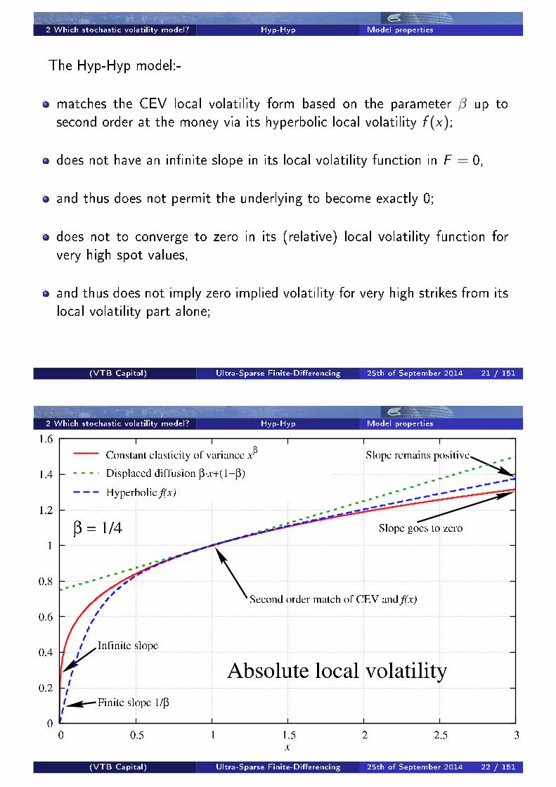
The Hyp-Hyp model:-
matches the CEV local volatility form based on the parameter β up tosecond order at the money via its hyperbolic local volatility f (x);
does not have an in�nite slope in its local volatility function in F = 0,
and thus does not permit the underlying to become exactly 0;
does not to converge to zero in its (relative) local volatility function forvery high spot values,
and thus does not imply zero implied volatility for very high strikes from itslocal volatility part alone;
(VTB Capital) Ultra-Sparse Finite-Di�erencing 25th of September 2014 21 / 151
2 Which stochastic volatility model? Hyp-Hyp Model properties
(VTB Capital) Ultra-Sparse Finite-Di�erencing 25th of September 2014 22 / 151

2 Which stochastic volatility model? Hyp-Hyp Model properties
(VTB Capital) Ultra-Sparse Finite-Di�erencing 25th of September 2014 23 / 151
2 Which stochastic volatility model? Hyp-Hyp Model properties
(VTB Capital) Ultra-Sparse Finite-Di�erencing 25th of September 2014 24 / 151
2 Which stochastic volatility model? Hyp-Hyp Negative β?
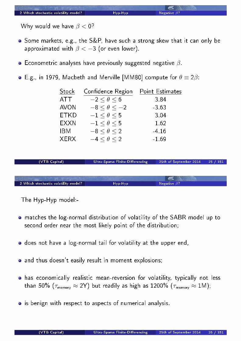
Why would we have β < 0?
Some markets, e.g., the S&P, have such a strong skew that it can only beapproximated with β < −3 (or even lower).
Econometric analyses have previously suggested negative β.
E.g., in 1979, Macbeth and Merville [MM80] compute for θ ≡ 2β:
Stock Con�dence Region Point Estimates
ATT −2 ≤ θ ≤ 6 3.84AVON −8 ≤ θ ≤ −2 -3.63ETKD −1 ≤ θ ≤ 5 3.04EXXN −1 ≤ θ ≤ 5 1.62IBM −8 ≤ θ ≤ 2 -4.16XERX −4 ≤ θ ≤ 2 -1.69
(VTB Capital) Ultra-Sparse Finite-Di�erencing 25th of September 2014 25 / 151
2 Which stochastic volatility model? Hyp-Hyp Negative β?
The Hyp-Hyp model:-
matches the log-normal distribution of volatility of the SABR model up tosecond order near the most likely point of the distribution;
does not have a log-normal tail for volatility at the upper end,
and thus doesn't easily result in moment explosions;
has economically realistic mean-reversion for volatility, typically not lessthan 50% (τmemory ≈ 2Y) but readily as high as 1200% (τmemory ≈ 1M);
is benign with respect to aspects of numerical analysis.
(VTB Capital) Ultra-Sparse Finite-Di�erencing 25th of September 2014 26 / 151
2 Which stochastic volatility model? Hyp-Hyp Negative β?
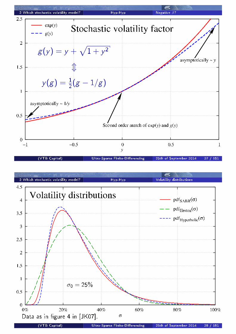
g(y) = y +√
1+ y 2
m
y(g) = 12(g − 1/g)
(VTB Capital) Ultra-Sparse Finite-Di�erencing 25th of September 2014 27 / 151
2 Which stochastic volatility model? Hyp-Hyp Volatility distributions
Data as in �gure 4 in [JK07].
σ0 = 25%
(VTB Capital) Ultra-Sparse Finite-Di�erencing 25th of September 2014 28 / 151
2 Which stochastic volatility model? Hyp-Hyp Volatility distributions
Data as in �gure 4 in [JK07].
σ0 = 25%
(VTB Capital) Ultra-Sparse Finite-Di�erencing 25th of September 2014 29 / 151
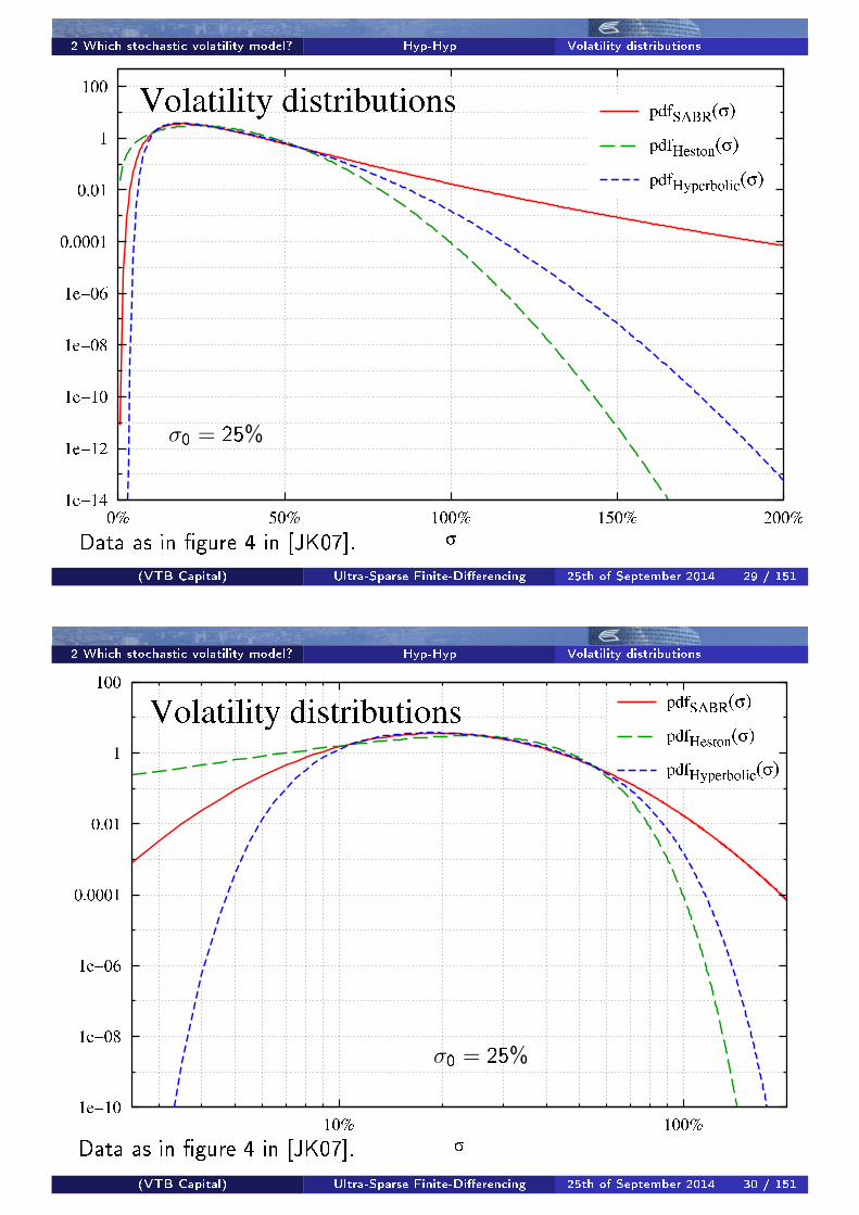
2 Which stochastic volatility model? Hyp-Hyp Volatility distributions
Data as in �gure 4 in [JK07].
σ0 = 25%
(VTB Capital) Ultra-Sparse Finite-Di�erencing 25th of September 2014 30 / 151

2 Which stochastic volatility model? Hyp-Hyp What about ZABR?
P. Hagan mentioned that the response of volatility to its factor should, on alogarithmic scale, only be about 80%.The suggestion was to use the ZABR [AH11] form for the volatility process:
dα̃ = α̃γ · dZ (1)
To compare this with the exponential form of SABR, and the hyperbolicform g(y) of Hyp-Hyp, we take, assuming for simplicity that α̃0 = 1,∫
α̃0
dα̃
α̃= ln α̃− ln α̃0 ⇒ α̃(z) ∼ e
z (2)∫α̃0
dα̃
α̃γ=
α̃1−γ − α̃1−γ0
1− γ⇒ α̃(z) ∼ [1 + (1− γ) · z ]
1(1−γ) (3)
to de�nezabr(z ; γ) := [1 + (1− γ) · z ]
1(1−γ) . (4)
What does this look like for γ = 80% in comparison to the SABR (exponen-tial) case, and how does g(·) compare?
(VTB Capital) Ultra-Sparse Finite-Di�erencing 25th of September 2014 31 / 151
2 Which stochastic volatility model? Hyp-Hyp What about ZABR?
Positive shocks (z > 0):Hyperbolic g(z) gives about the same(reduced) de�ection as a γ = 0.8 ZABRform for a signi�cant factor shock size z!
(VTB Capital) Ultra-Sparse Finite-Di�erencing 25th of September 2014 32 / 151
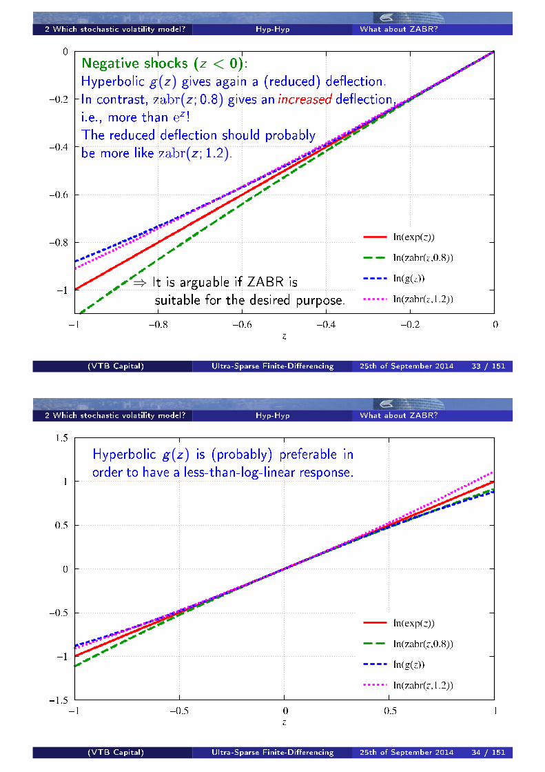
2 Which stochastic volatility model? Hyp-Hyp What about ZABR?
Negative shocks (z < 0):Hyperbolic g(z) gives again a (reduced) de�ection.In contrast, zabr(z ; 0.8) gives an increased de�ection,i.e., more than e
z !The reduced de�ection should probablybe more like zabr(z ; 1.2).
⇒ It is arguable if ZABR issuitable for the desired purpose.
(VTB Capital) Ultra-Sparse Finite-Di�erencing 25th of September 2014 33 / 151
2 Which stochastic volatility model? Hyp-Hyp What about ZABR?
Hyperbolic g(z) is (probably) preferable inorder to have a less-than-log-linear response.
(VTB Capital) Ultra-Sparse Finite-Di�erencing 25th of September 2014 34 / 151
3 The DHI volatility framework Scope
The scope of the DHI volatility framework
is to:-
take in parameters de�ned in terms of the HypHyp local-stochastic volatilityprocess,
output implied volatilities at a computational performance that is not sig-ni�cantly di�erent from the use of an actual analytical formula,
be completely free of arbitrage, without any exceptions,
provide a wide range of smile and skew shapes,
be amenable to specifying term structures of (piecewise constant) param-eter values to create a complete volatility surface that is by constructionfree of arbitrage.
(VTB Capital) Ultra-Sparse Finite-Di�erencing 25th of September 2014 35 / 151
3 The DHI volatility framework The parameters
Meaning of the parameters
σ0: initial level of instantaneous volatility. Approximately equal to shortterm ATF implied volatility.LEVEL.
β: local volatility skew coe�cients. Same purpose and behaviour as inCEV or SABR.SKEW (via local volatility).
α: uncertainty of volatility in the sense of relative standard deviation. Thisis not volatility of volatility1. Recall that volatility scales by e
y and that αis the width of the stationary distribution of y .SMILE (via stochastic volatility).
1Volatility of volatility is α√2κ but this quantity is often misleading in a
mean-reverting context.(VTB Capital) Ultra-Sparse Finite-Di�erencing 25th of September 2014 36 / 151
3 The DHI volatility framework The parameters
ρ: correlation of the spot process driver di�usion and the volatilit processdriver di�usion. Same purpose and behaviour as in SABR or Heston, etc.SKEW (via stochastic volatility).
κ: mean reversion of volatility. May need to be> 100% to straighten smilesor to accommodate long term volatility being not signi�cantly higher thanshort term, as well as reduction of long term smile (which is something thatSABR cannot match).
Larger κ makes y converge to the stationary distribution more rapidly.
Volatility memory time: τmemory ∼1
κ.
STRAIGHTENING (both in the strike direction and in time).
(VTB Capital) Ultra-Sparse Finite-Di�erencing 25th of September 2014 37 / 151
3 The DHI volatility framework Spatial discretisation
We de�ne the DHI frameworkon a spatial discretisation for the process of the underlying, and of volatility.
To be crystal clear: our design is not an approximation to any processthat is de�ned on a (spatially) continuous domain.
We de�ne a process with stochastic volatility on a discrete set ofspatial levels, both for the �nancial underlying, and for volatility.
This means that the chosen number of discrete levels is technically part ofthe set of parameters.
In practice, we use 25× 11 nodes throughout.
DHI calculations are mathematically equivalent to acontinuous-time-�nite-state Markov chain.
(VTB Capital) Ultra-Sparse Finite-Di�erencing 25th of September 2014 38 / 151
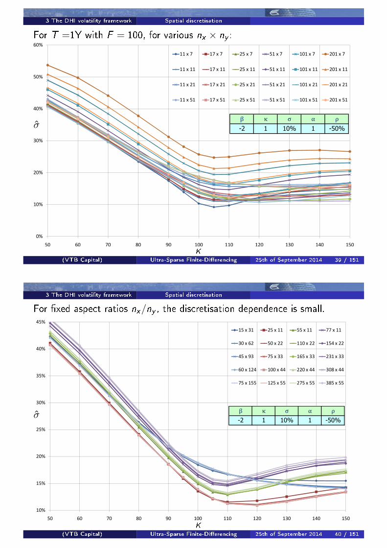
3 The DHI volatility framework Spatial discretisation
For T =1Y with F = 100, for various nx × ny :
��
���
���
���
���
���
���
�� �� �� � � ��� ��� ��� ��� ��� ���
������ ������ ������ ������ ������� �������
������� ������� ������� ������� �������� ��������
������� ������� ������� ������� �������� ��������
������� ������� ������� ������� �������� ��������
K
σ̂� � � � �
�� � ��� � ����
(VTB Capital) Ultra-Sparse Finite-Di�erencing 25th of September 2014 39 / 151
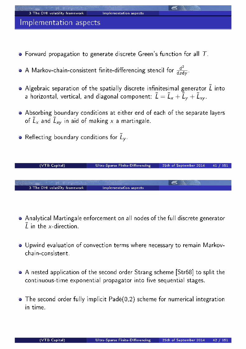
3 The DHI volatility framework Spatial discretisation
For �xed aspect ratios nx/ny , the discretisation dependence is small.
���
���
���
���
���
���
���
���
�� �� �� � � ��� ��� ��� ��� ��� ���
������� ������� ������� �������
������� ������� �������� ��������
������ ������� �������� ��������
�������� �������� �������� �������
�������� �������� �������� �������
K
σ̂ � � � � �
�� � ��� � ����
(VTB Capital) Ultra-Sparse Finite-Di�erencing 25th of September 2014 40 / 151
3 The DHI volatility framework Implementation aspects
Implementation aspects
Forward propagation to generate discrete Green's function for all T .
A Markov-chain-consistent �nite-di�erencing stencil for d2
dzdy .
Algebraic separation of the spatially discrete in�nitesimal generator L̃ intoa horizontal, vertical, and diagonal component: L̃ = L̃x + L̃y + L̃xy .
Absorbing boundary conditions at either end of each of the separate layersof L̃x and L̃xy in aid of making x a martingale.
Re�ecting boundary conditions for L̃y .
(VTB Capital) Ultra-Sparse Finite-Di�erencing 25th of September 2014 41 / 151
3 The DHI volatility framework Implementation aspects
Analytical Martingale enforcement on all nodes of the full discrete generatorL̃ in the x-direction.
Upwind evaluation of convection terms where necessary to remain Markov-chain-consistent.
A nested application of the second order Strang scheme [Str68] to split thecontinuous-time exponential propagator into �ve sequential stages.
The second order fully implicit Padé(0,2) scheme for numerical integrationin time.
(VTB Capital) Ultra-Sparse Finite-Di�erencing 25th of September 2014 42 / 151
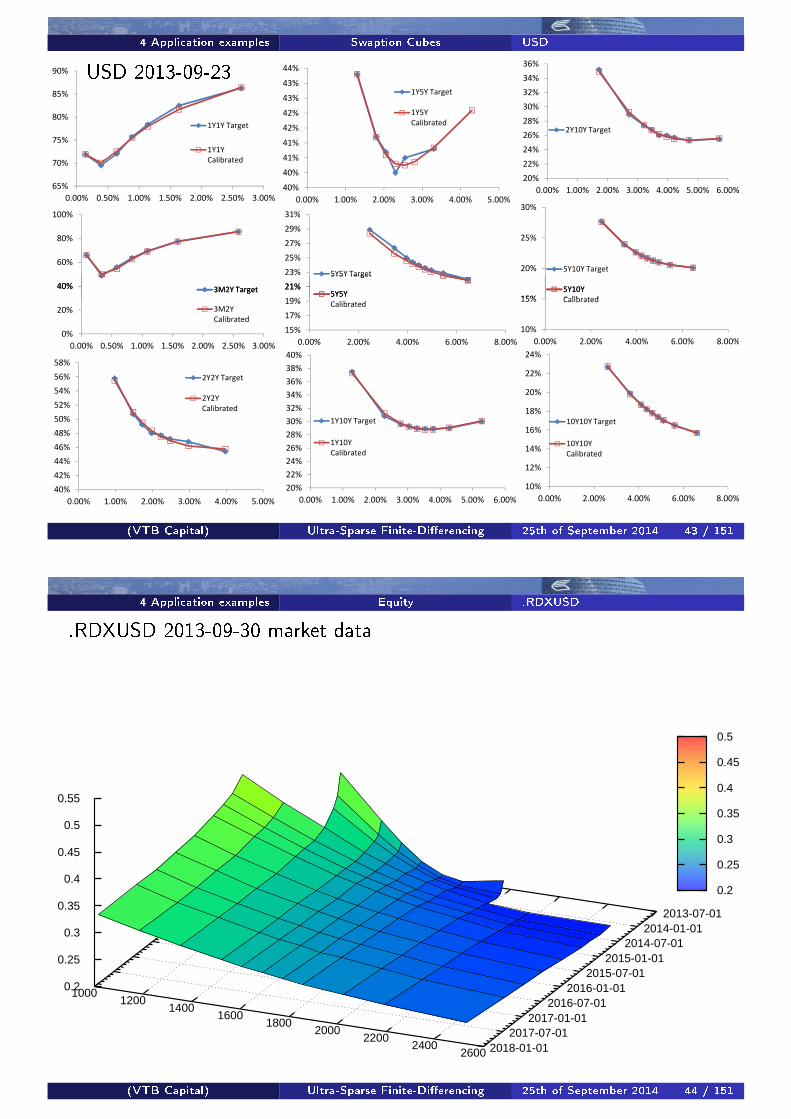
4 Application examples Swaption Cubes USD
65%
70%
75%
80%
85%
90%
0.00% 0.50% 1.00% 1.50% 2.00% 2.50% 3.00%
1Y1Y Target
1Y1Y
Calibrated
40%
60%
80%
100%
3M2Y Target
40%
40%
41%
41%
42%
42%
43%
43%
44%
0.00% 1.00% 2.00% 3.00% 4.00% 5.00%
1Y5Y Target
1Y5Y
Calibrated
19%
21%
23%
25%
27%
29%
31%
5Y5Y Target
5Y5Y
20%
22%
24%
26%
28%
30%
32%
34%
36%
0.00% 1.00% 2.00% 3.00% 4.00% 5.00% 6.00%
2Y10Y Target
15%
20%
25%
30%
5Y10Y Target
5Y10Y
Calibrated
0%
20%
40%
0.00% 0.50% 1.00% 1.50% 2.00% 2.50% 3.00%
3M2Y Target
3M2Y
Calibrated
40%
42%
44%
46%
48%
50%
52%
54%
56%
58%
0.00% 1.00% 2.00% 3.00% 4.00% 5.00%
2Y2Y Target
2Y2Y
Calibrated
20%
22%
24%
26%
28%
30%
32%
34%
36%
38%
40%
0.00% 1.00% 2.00% 3.00% 4.00% 5.00% 6.00%
1Y10Y Target
1Y10Y
Calibrated
15%
17%
19%
21%
23%
0.00% 2.00% 4.00% 6.00% 8.00%
5Y5Y Target
5Y5Y
Calibrated
10%
15%
0.00% 2.00% 4.00% 6.00% 8.00%
5Y10Y
Calibrated
10%
12%
14%
16%
18%
20%
22%
24%
0.00% 2.00% 4.00% 6.00% 8.00%
10Y10Y Target
10Y10Y
Calibrated
USD 2013-09-23
(VTB Capital) Ultra-Sparse Finite-Di�erencing 25th of September 2014 43 / 151
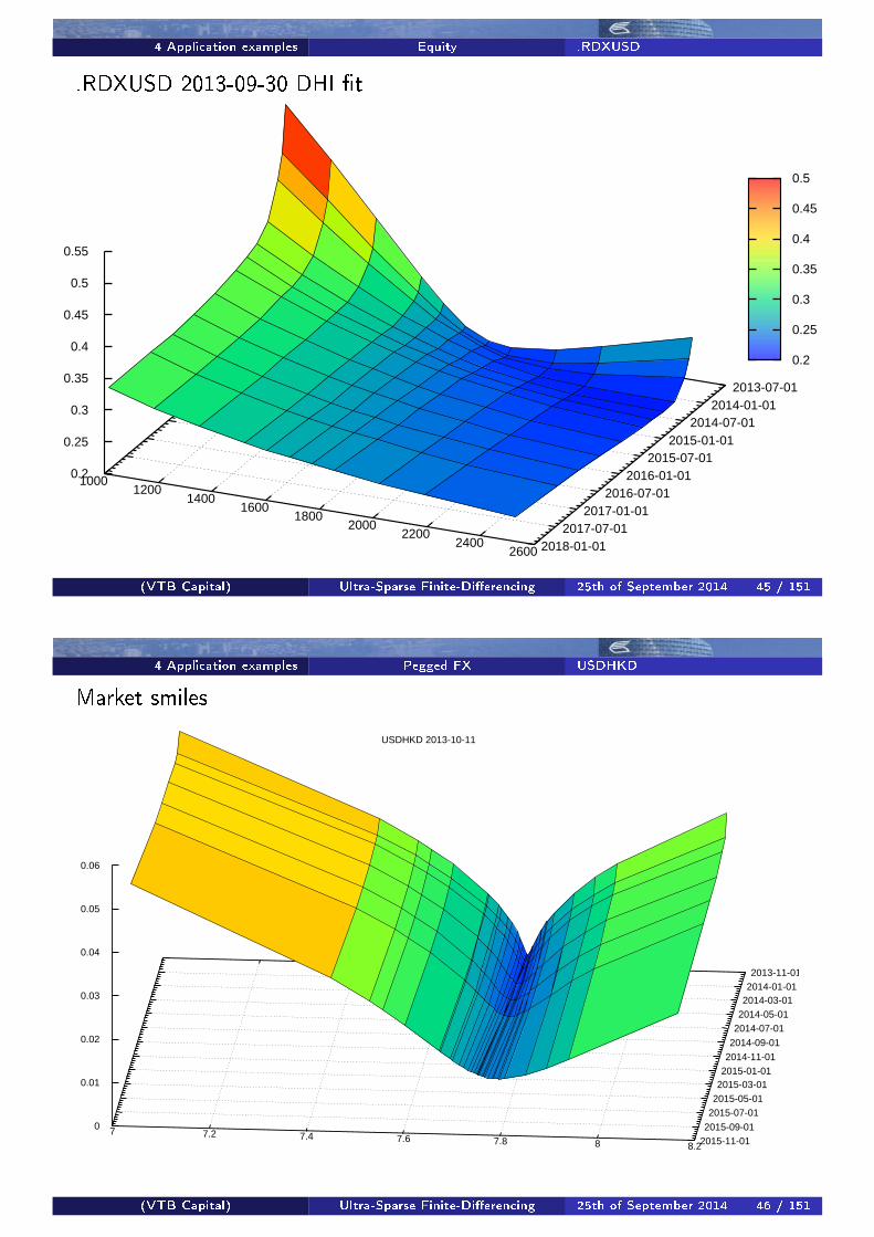
4 Application examples Equity .RDXUSD
.RDXUSD 2013-09-30 market data
1000 1200
1400 1600
1800 2000
2200 2400
2600
2013-07-012014-01-01
2014-07-012015-01-01
2015-07-012016-01-01
2016-07-012017-01-01
2017-07-012018-01-01
0.2
0.25
0.3
0.35
0.4
0.45
0.5
0.55
0.2
0.25
0.3
0.35
0.4
0.45
0.5
(VTB Capital) Ultra-Sparse Finite-Di�erencing 25th of September 2014 44 / 151
4 Application examples Equity .RDXUSD
.RDXUSD 2013-09-30 DHI �t
1000 1200
1400 1600
1800 2000
2200 2400
2600
2013-07-012014-01-01
2014-07-012015-01-01
2015-07-012016-01-01
2016-07-012017-01-01
2017-07-012018-01-01
0.2
0.25
0.3
0.35
0.4
0.45
0.5
0.55
0.2
0.25
0.3
0.35
0.4
0.45
0.5
(VTB Capital) Ultra-Sparse Finite-Di�erencing 25th of September 2014 45 / 151
4 Application examples Pegged FX USDHKD
Market smiles
7 7.2 7.4 7.6 7.8 8 8.2
2013-11-012014-01-01
2014-03-012014-05-01
2014-07-01
2014-09-01
2014-11-012015-01-01
2015-03-012015-05-01
2015-07-01
2015-09-012015-11-01
0
0.01
0.02
0.03
0.04
0.05
0.06
USDHKD 2013-10-11
(VTB Capital) Ultra-Sparse Finite-Di�erencing 25th of September 2014 46 / 151
4 Application examples Pegged FX USDHKD
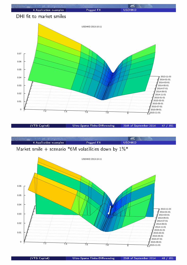
DHI �t to market smiles
7 7.2 7.4 7.6 7.8 8 8.2
2013-11-012014-01-01
2014-03-012014-05-01
2014-07-01
2014-09-01
2014-11-012015-01-01
2015-03-012015-05-01
2015-07-01
2015-09-012015-11-01
0
0.01
0.02
0.03
0.04
0.05
0.06
0.07
USDHKD 2013-10-11
(VTB Capital) Ultra-Sparse Finite-Di�erencing 25th of September 2014 47 / 151
4 Application examples Pegged FX USDHKD
Market smile + scenario "6M volatilities down by 1%"
7 7.2 7.4 7.6 7.8 8 8.2
2013-11-012014-01-01
2014-03-012014-05-01
2014-07-01
2014-09-01
2014-11-012015-01-01
2015-03-012015-05-01
2015-07-01
2015-09-012015-11-01
0
0.01
0.02
0.03
0.04
0.05
0.06
USDHKD 2013-10-11
(VTB Capital) Ultra-Sparse Finite-Di�erencing 25th of September 2014 48 / 151
4 Application examples Pegged FX USDHKD
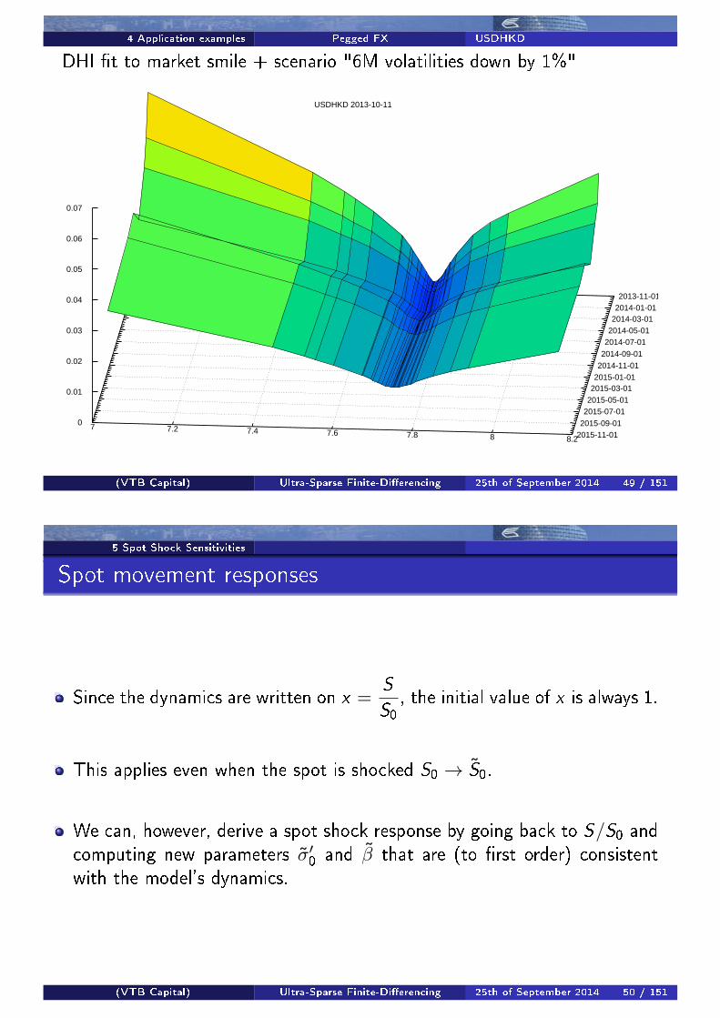
DHI �t to market smile + scenario "6M volatilities down by 1%"
7 7.2 7.4 7.6 7.8 8 8.2
2013-11-012014-01-01
2014-03-012014-05-01
2014-07-01
2014-09-01
2014-11-012015-01-01
2015-03-012015-05-01
2015-07-01
2015-09-012015-11-01
0
0.01
0.02
0.03
0.04
0.05
0.06
0.07
USDHKD 2013-10-11
(VTB Capital) Ultra-Sparse Finite-Di�erencing 25th of September 2014 49 / 151
5 Spot Shock Sensitivities
Spot movement responses
Since the dynamics are written on x =S
S0, the initial value of x is always 1.
This applies even when the spot is shocked S0 → S̃0.
We can, however, derive a spot shock response by going back to S/S0 andcomputing new parameters σ̃′0 and β̃ that are (to �rst order) consistentwith the model's dynamics.
(VTB Capital) Ultra-Sparse Finite-Di�erencing 25th of September 2014 50 / 151

5 Spot Shock Sensitivities Parametric Response
The absolute volatility σabs of the spot S ≡ Ft(t) is given by:
σabs(S ,Ft(0), σ0, β) := σ0 · Ft(0) · f ( SFt(0) ;β) · g(y). (5)
If the forward curve moves from Ft(0) to F̃t(0), we look for σ̃0 and β̃ suchthat:
σabs(S ,Ft(0), σ0, β)∣∣∣S=F̃t(0)
= σabs(S , F̃t(0), σ̃0, β̃)∣∣∣S=F̃t(0)
(6)
∂Sσabs(S ,Ft(0), σ0, β)∣∣∣S=F̃t(0)
= ∂Sσabs(S , F̃t(0), σ̃0, β̃)∣∣∣S=F̃t(0)
(7)
Denoting x̃ := F̃t(0)Ft(0) , we obtain the analytical solution
σ̃0 = σ0 · f (x̃ ;β)/x̃ (8)
β̃ = x̃ · ∂x ln f (x ;β)∣∣∣x=x̃
. (9)
(VTB Capital) Ultra-Sparse Finite-Di�erencing 25th of September 2014 51 / 151
5 Spot Shock Sensitivities Dynamic Delta
The �exibility of the DHI framework allows us to match virtually the samesmile for di�erent values of β.
Di�erent choices of parameters give rise to di�erent vega-adjusted Deltas
∆ =∂B
∂S0+∂σ̂
∂S0
∂B
∂σ̂(10)
where B is the Black or Bachelier formula, and σ̂ is implied volatility.
P. Hagan [Hag13] observed that, with a model-consistent response ∂σ̂∂S0
, weare largely immunized against di�erent parametrisations of the same smile.
(VTB Capital) Ultra-Sparse Finite-Di�erencing 25th of September 2014 52 / 151
5 Spot Shock Sensitivities Dynamic Delta
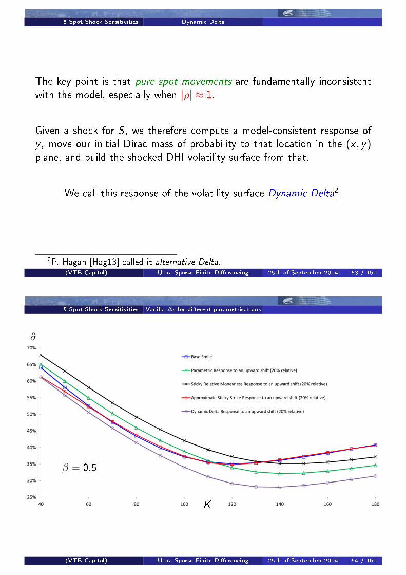
The key point is that pure spot movements are fundamentally inconsistentwith the model, especially when |ρ| ≈ 1.
Given a shock for S , we therefore compute a model-consistent response ofy , move our initial Dirac mass of probability to that location in the (x , y)plane, and build the shocked DHI volatility surface from that.
We call this response of the volatility surface Dynamic Delta2.
2P. Hagan [Hag13] called it alternative Delta.(VTB Capital) Ultra-Sparse Finite-Di�erencing 25th of September 2014 53 / 151
5 Spot Shock Sensitivities Vanilla ∆s for di�erent parametrisations
25%
30%
35%
40%
45%
50%
55%
60%
65%
70%
40 60 80 100 120 140 160 180
Base Smile
Parametric Response to an upward shift (20% relative)
Sticky Relative Moneyness Response to an upward shift (20% relative)
Approximate Sticky Strike Response to an upward shift (20% relative)
Dynamic Delta Response to an upward shift (20% relative)
K
σ̂
β = 0.5
(VTB Capital) Ultra-Sparse Finite-Di�erencing 25th of September 2014 54 / 151
5 Spot Shock Sensitivities Vanilla ∆s for di�erent parametrisations
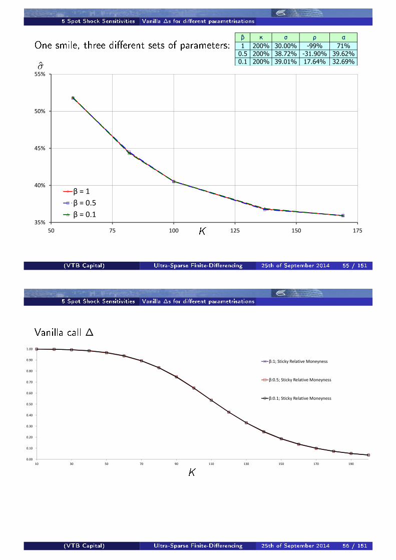
One smile, three di�erent sets of parameters:
50%
55%
35%
40%
45%
50 75 100 125 150 175
β = 1
β = 0.5
β = 0.1
K
σ̂
β κ σ ρ α
1 200% 30.00% -99% 71%
0.5 200% 38.72% -31.90% 39.62%
0.1 200% 39.01% 17.64% 32.69%
(VTB Capital) Ultra-Sparse Finite-Di�erencing 25th of September 2014 55 / 151
5 Spot Shock Sensitivities Vanilla ∆s for di�erent parametrisations
Vanilla call ∆
0.00
0.10
0.20
0.30
0.40
0.50
0.60
0.70
0.80
0.90
1.00
10 30 50 70 90 110 130 150 170 190
β:1; Sticky Relative Moneyness
β:0.5; Sticky Relative Moneyness
β:0.1; Sticky Relative Moneyness
K
(VTB Capital) Ultra-Sparse Finite-Di�erencing 25th of September 2014 56 / 151

5 Spot Shock Sensitivities Vanilla ∆s for di�erent parametrisations
Vanilla call ∆
0.00
0.10
0.20
0.30
0.40
0.50
0.60
0.70
0.80
0.90
1.00
10 30 50 70 90 110 130 150 170 190
β:1; Approximate Sticky Strike
β:0.5; Approximate Sticky Strike
β:0.1; Approximate Sticky Strike
K
(via recalibration)
(VTB Capital) Ultra-Sparse Finite-Di�erencing 25th of September 2014 57 / 151
5 Spot Shock Sensitivities Vanilla ∆s for di�erent parametrisations
Vanilla call ∆
0.00
0.10
0.20
0.30
0.40
0.50
0.60
0.70
0.80
0.90
1.00
10 30 50 70 90 110 130 150 170 190
β:1; Parametric Response
β:0.5; Parametric Response
β:0.1; Parametric Response
K
(VTB Capital) Ultra-Sparse Finite-Di�erencing 25th of September 2014 58 / 151

5 Spot Shock Sensitivities Vanilla ∆s for di�erent parametrisations
Vanilla call ∆
0.00
0.10
0.20
0.30
0.40
0.50
0.60
0.70
0.80
0.90
1.00
10 30 50 70 90 110 130 150 170 190
β:1; Dynamic Delta
β:0.5; Dynamic Delta
β:0.1; Dynamic Delta
K
(VTB Capital) Ultra-Sparse Finite-Di�erencing 25th of September 2014 59 / 151
5 Spot Shock Sensitivities Vanilla ∆s for di�erent parametrisations
Vanilla call ∆
0.00
0.10
0.20
0.30
0.40
0.50
0.60
0.70
0.80
0.90
1.00
10 30 50 70 90 110 130 150 170 190
β:0.5; Sticky Relative Moneyness
β:0.5; Approximate Sticky Strike
β:0.5; Parametric Response
β:0.5; Dynamic Delta
K
Deltas from four di�erent response types.
(VTB Capital) Ultra-Sparse Finite-Di�erencing 25th of September 2014 60 / 151
5 Spot Shock Sensitivities Calibration to spot-vol slope
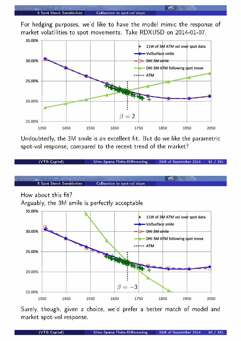
For hedging purposes, we'd like to have the model mimic the response ofmarket volatilities to spot movements. Take RDXUSD on 2014-01-07.
������
������
������
��������� �����������������
��������������
������������
�������� ���� �!"��������
� �
������
������
������
������
������
���� �#�� ���� �$�� �%�� �&�� �'�� ����
��������� �����������������
��������������
������������
�������� ���� �!"��������
� �
β = 2
Undoubtedly, the 3M smile is an excellent �t. But do we like the parametricspot-vol response, compared to the recent trend of the market?
(VTB Capital) Ultra-Sparse Finite-Di�erencing 25th of September 2014 61 / 151
5 Spot Shock Sensitivities Calibration to spot-vol slope
How about this �t?Arguably, the 3M smile is perfectly acceptable.
������
������
������
��������� �����������������
��������������
������������
�������� ���� �!"��������
� �
������
������
������
������
������
���� �#�� ���� �$�� �%�� �&�� �'�� ����
��������� �����������������
��������������
������������
�������� ���� �!"��������
� �
β = −3
Surely, though, given a choice, we'd prefer a better match of model andmarket spot-vol response.
(VTB Capital) Ultra-Sparse Finite-Di�erencing 25th of September 2014 62 / 151
5 Spot Shock Sensitivities Calibration to spot-vol slope
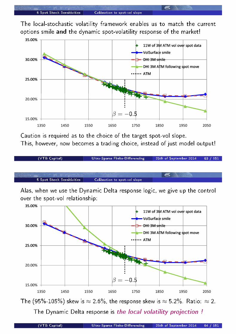
The local-stochastic volatility framework enables us to match the currentoptions smile and the dynamic spot-volatility response of the market!
������
������
������
��������� �����������������
��������������
������������
�������� ���� �!"��������
� �
������
������
������
������
������
���� �#�� ���� �$�� �%�� �&�� �'�� ����
��������� �����������������
��������������
������������
�������� ���� �!"��������
� �
β = −0.5
Caution is required as to the choice of the target spot-vol slope.This, however, now becomes a trading choice, instead of just model output!
(VTB Capital) Ultra-Sparse Finite-Di�erencing 25th of September 2014 63 / 151
5 Spot Shock Sensitivities Calibration to spot-vol slope
Alas, when we use the Dynamic Delta response logic, we give up the controlover the spot-vol relationship:
������
������
������
��������� �����������������
��������������
������������
�������� ���� �!"��������
� �
������
������
������
������
������
���� �#�� ���� �$�� �%�� �&�� �'�� ����
��������� �����������������
��������������
������������
�������� ���� �!"��������
� �
β = −0.5
The (95%-105%) skew is ≈ 2.6%, the response skew is ≈ 5.2%. Ratio: ≈ 2.
The Dynamic Delta response is the local volatility projection !
(VTB Capital) Ultra-Sparse Finite-Di�erencing 25th of September 2014 64 / 151
5 Spot Shock Sensitivities Calibration to spot-vol slope
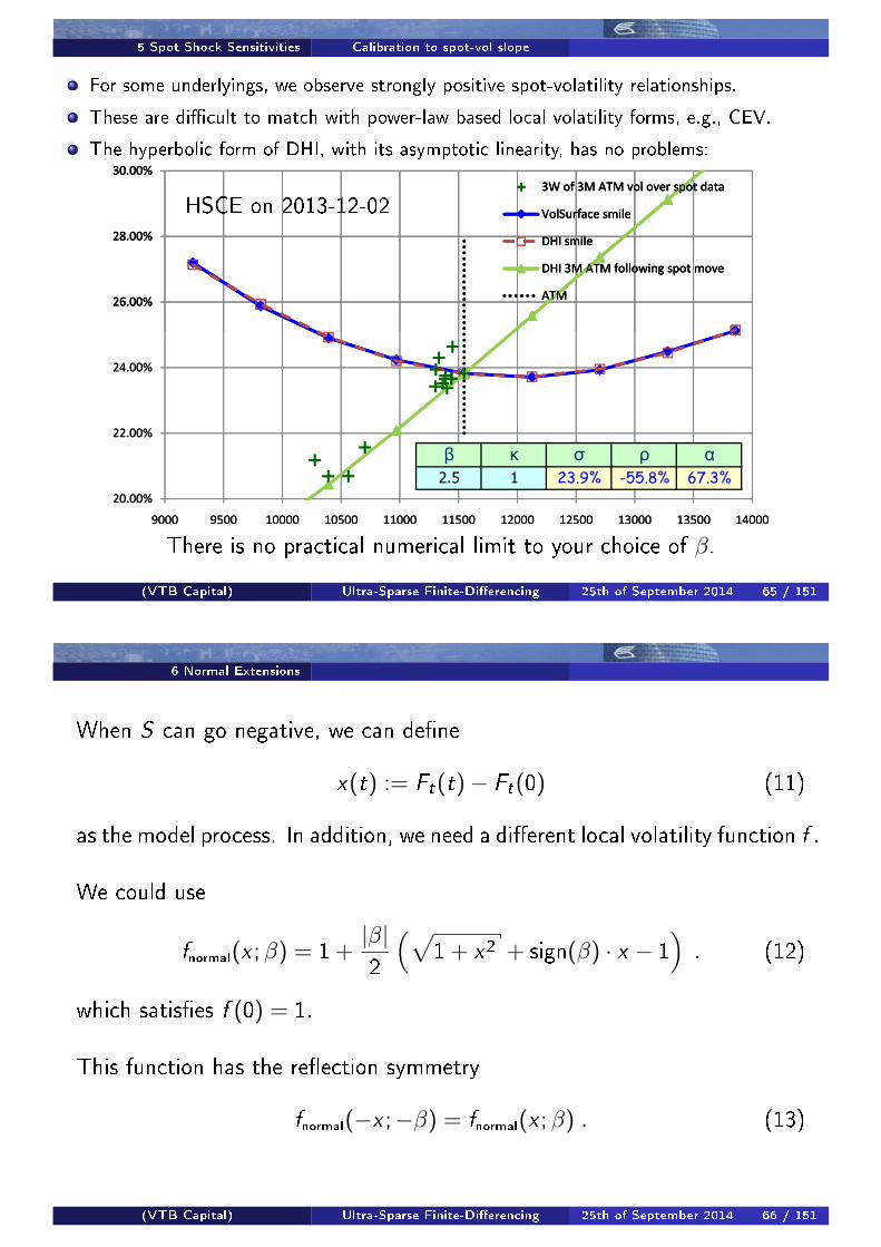
For some underlyings, we observe strongly positive spot-volatility relationships.
These are di�cult to match with power-law based local volatility forms, e.g., CEV.
The hyperbolic form of DHI, with its asymptotic linearity, has no problems:
������
������
������
�������� �����������������
��������������
���������
�������� ���� �!"��������
� �
������
������
�#����
������
������
������
$��� $%�� &���� &�%�� &&��� &&%�� &���� &�%�� &���� &�%�� &#���
�������� �����������������
��������������
���������
�������� ���� �!"��������
� �
������
������
�#����
������
������
������
$��� $%�� &���� &�%�� &&��� &&%�� &���� &�%�� &���� &�%�� &#���
�������� �����������������
��������������
���������
�������� ���� �!"��������
� �
HSCE on 2013-12-02
� � � � �
��� � ����� ������ ����
There is no practical numerical limit to your choice of β.
(VTB Capital) Ultra-Sparse Finite-Di�erencing 25th of September 2014 65 / 151
6 Normal Extensions
When S can go negative, we can de�ne
x(t) := Ft(t)− Ft(0) (11)
as the model process. In addition, we need a di�erent local volatility function f .
We could use
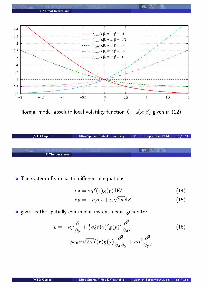
fnormal(x ;β) = 1 +|β|2
(√1 + x2 + sign(β) · x − 1
). (12)
which satis�es f (0) = 1.
This function has the re�ection symmetry
fnormal(−x ;−β) = fnormal(x ;β) . (13)
(VTB Capital) Ultra-Sparse Finite-Di�erencing 25th of September 2014 66 / 151
6 Normal Extensions
Normal model absolute local volatility function fnormal(x ;β) given in (12).
(VTB Capital) Ultra-Sparse Finite-Di�erencing 25th of September 2014 67 / 151
7 The generator
The system of stochastic di�erential equations
dx = σ0f (x)g(y)dW (14)
dy = −κydt + α√2κ dZ (15)
gives us the spatially continuous instantaneous generator
L = −κy ∂
∂y+ 1
2σ20f (x)2g(y)2
∂2
∂x2(16)
+ ρσ0α√2κ f (x)g(y)
∂2
∂x∂y+ κα2
∂2
∂y2
(VTB Capital) Ultra-Sparse Finite-Di�erencing 25th of September 2014 68 / 151

7 The generator
Pricing derivatives �backward Kolmogorov equation:
∂∂T v = −L · v . (17)
Transition probabilities from t = 0 to T �forward Kolmogorov or Fokker-Planck equation:
∂∂t p = L∗ · p . (18)
=⇒ L∗ is the adjoint of the operator L.
Starting from a Dirac spike at t = 0, this gives us
Green's functions.
(VTB Capital) Ultra-Sparse Finite-Di�erencing 25th of September 2014 69 / 151
7 The generator Spot-logarithmic coordinates
Transform to the logarithmic coordinate
z := ln(x) . (19)
The generator L becomes
L = −12ς(z , y)2
∂
∂z− κy ∂
∂y(20)
+ 12ς(z , y)2
∂2
∂z2+ ρς(z , y)α
√2κ
∂2
∂z∂y+ κα2
∂2
∂y2
with the time-homogenous separable local (in z and y) volatility
ς(z , y) := σ0 e−z f (ez)g(y) . (21)
(VTB Capital) Ultra-Sparse Finite-Di�erencing 25th of September 2014 70 / 151
8 Spatial discretisation
We form a lattice of (typically) nz = 25× ny = 11 spatial nodes.
The dynamics are con�ned to these spatial levels.
The operator L is replaced by a spatially discretised generator L̃by the aid of �nite di�erencing stencils.
The probability function p(t, z , y) becomes a vector-valued function of timealone
p̃(t) ∈ Rnz×ny .
=⇒ p̃(t) is still continuous in time.
(VTB Capital) Ultra-Sparse Finite-Di�erencing 25th of September 2014 71 / 151
8 Spatial discretisation Continuous-time �nite-state Markov
The (forward) dynamics are now governed by the
system of ordinary di�erential equations
∂∂t p̃ = L̃∗ · p̃ (22)
with solution
p̃(t + τ) = eτ ·L̃∗· p̃(t) (23)
The dynamics are now exactly in the form of a
continuous-time �nite-state Markov chain.
(VTB Capital) Ultra-Sparse Finite-Di�erencing 25th of September 2014 72 / 151
8 Spatial discretisation Continuous-time �nite-state Markov The Metzler property
Since L̃ is a real-valued matrix,
L̃∗ = L̃> .
Choose boundary conditions for the generator L̃, and L̃∗ follows trivially!
(This is a common problem when implementing the forward-Kolmogorov system: what
boundary conditions to use in a forward scheme? As we show here, it shouldn't be an
issue at all.)
From eτ ·L̃∗· p̃, we see that L̃ must not have any eigenvalues with positive
real parts: sup{<(λ) : λ ∈ Σ(L̃)
}≤ 0 (24)
Since the rows of L̃ always sum up to zero (Markov chain property), for (24)to hold, via the Gershgorin circle theorem,
it is su�cient that all o�-diagonal elements of L̃ are ≥ 0.
This is known as the Metzler property.
⇒ The spatial discretisation and boundary conditions must result inL̃ being a Metzler matrix.
(VTB Capital) Ultra-Sparse Finite-Di�erencing 25th of September 2014 73 / 151
8 Spatial discretisation Continuous-time �nite-state Markov The Metzler property
The generator L̃ is also know under the names transition rate matrix orintensity matrix.
The dynamics are a pure jump process with nearest-neighbour-transitions.
We can compute the (residual) drift in the x-direction from Itô'slemma for pure jump processes.
We can use this knowledge to make L̃ an analytically exact x-martingale.
This COMPLETELY removes any residual drift error as is commonlyobserved in �nite-di�erencing schemes.
This residual drift is the dominant reason why most �nite-di�erencing implementations
need signi�cant numbers (at least hundreds, but even thousands) of discretisation levels
in the spot (x) direction.
We can have L̃ as a perfect x-martingale with any number of nodes, be it100, 10, or even just 3!
(VTB Capital) Ultra-Sparse Finite-Di�erencing 25th of September 2014 74 / 151
9 Continuous-time perfect martingale Local volatility example
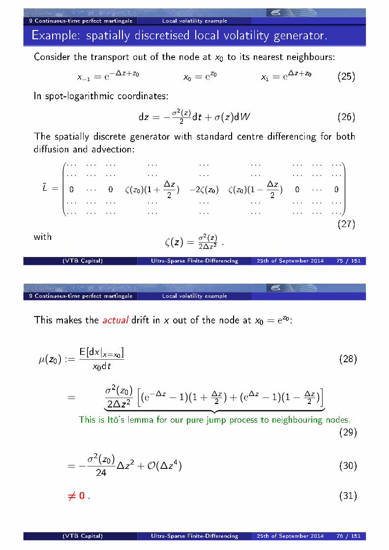
Example: spatially discretised local volatility generator.
Consider the transport out of the node at x0 to its nearest neighbours:
x−1 = e−∆z+z0 x0 = e
z0 x1 = e∆z+z0 (25)
In spot-logarithmic coordinates:
dz = −σ2(z)2
dt + σ(z)dW (26)
The spatially discrete generator with standard centre di�erencing for bothdi�usion and advection:
L̃ =
· · · · · · · · · · · · · · · · · · · · · · · · · · ·· · · · · · · · · · · · · · · · · · · · · · · · · · ·
0 · · · 0 ζ(z0)(1 +∆z
2) −2ζ(z0) ζ(z0)(1− ∆z
2) 0 · · · 0
· · · · · · · · · · · · · · · · · · · · · · · · · · ·· · · · · · · · · · · · · · · · · · · · · · · · · · ·
(27)
with ζ(z) = σ2(z)2∆z2
.
(VTB Capital) Ultra-Sparse Finite-Di�erencing 25th of September 2014 75 / 151
9 Continuous-time perfect martingale Local volatility example
This makes the actual drift in x out of the node at x0 = ez0 :
µ(z0) :=E[dx |x=x0 ]
x0dt(28)
=σ2(z0)
2∆z2
[(e−∆z − 1)(1 + ∆z
2) + (e∆z − 1)(1− ∆z
2)]
︸ ︷︷ ︸This is Itô's lemma for our pure jump process to neighbouring nodes.
(29)
= −σ2(z0)
24∆z2 +O(∆z4) (30)
6= 0 . (31)
(VTB Capital) Ultra-Sparse Finite-Di�erencing 25th of September 2014 76 / 151
9 Continuous-time perfect martingale Local volatility example
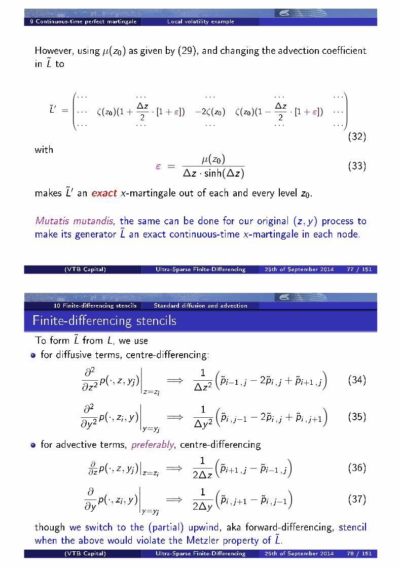
However, using µ(z0) as given by (29), and changing the advection coe�cientin L̃ to
L̃′ =
· · · · · · · · · · · · · · ·
· · · ζ(z0)(1 +∆z
2· [1 + ε]) −2ζ(z0) ζ(z0)(1− ∆z
2· [1 + ε]) · · ·
· · · · · · · · · · · · · · ·
(32)
with
ε =µ(z0)
∆z · sinh(∆z)(33)
makes L̃′ an exact x-martingale out of each and every level z0.
Mutatis mutandis, the same can be done for our original (z , y) process tomake its generator L̃ an exact continuous-time x-martingale in each node.
(VTB Capital) Ultra-Sparse Finite-Di�erencing 25th of September 2014 77 / 151
10 Finite-di�erencing stencils Standard di�usion and advection
Finite-di�erencing stencils
To form L̃ from L, we use
for di�usive terms, centre-di�erencing:
∂2
∂z2p(·, z , yj)
∣∣∣∣z=zi
=⇒ 1
∆z2
(p̃i−1 , j − 2p̃i , j + p̃i+1 , j
)(34)
∂2
∂y2p(·, zi , y)
∣∣∣∣y=yj
=⇒ 1
∆y2
(p̃i , j−1 − 2p̃i , j + p̃i , j+1
)(35)
for advective terms, preferably, centre-di�erencing
∂∂z p(·, z , yj)
∣∣z=zi
=⇒ 1
2∆z
(p̃i+1 , j − p̃i−1 , j
)(36)
∂
∂yp(·, zi , y)
∣∣∣∣y=yj
=⇒ 1
2∆y
(p̃i , j+1 − p̃i , j−1
)(37)
though we switch to the (partial) upwind, aka forward-di�erencing, stencilwhen the above would violate the Metzler property of L̃.
(VTB Capital) Ultra-Sparse Finite-Di�erencing 25th of September 2014 78 / 151
10 Finite-di�erencing stencils Cross-di�usion The Seven Point Stencil
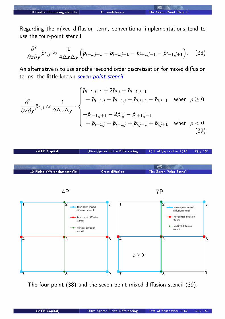
Regarding the mixed di�usion term, conventional implementations tend touse the four-point stencil
∂2
∂z∂yp̃i , j ≈
1
4∆z∆y
(p̃i+1,j+1 + p̃i−1,j−1 − p̃i+1,j−1 − p̃i−1,j+1
). (38)
An alternative is to use another second order discretisation for mixed di�usionterms, the little known seven-point stencil
∂2
∂z∂yp̃i , j ≈
1
2∆z∆y·
p̃i+1,j+1 + 2p̃i ,j + p̃i−1,j−1
− p̃i+1,j − p̃i−1,j − p̃i ,j+1 − p̃i ,j−1 when ρ ≥ 0
−p̃i−1,j+1 − 2p̃i ,j − p̃i+1,j−1
+ p̃i+1,j + p̃i−1,j + p̃i ,j−1 + p̃i ,j+1 when ρ < 0
(39)
(VTB Capital) Ultra-Sparse Finite-Di�erencing 25th of September 2014 79 / 151
10 Finite-di�erencing stencils Cross-di�usion The Seven Point Stencil
4P 7P
four-point mixed
diffusion stencil
horizontal diffusion
stencil
vertical diffusion
stencil
seven-point mixed
diffusion stencil
horizontal diffusion
stencil
vertical diffusion
stencil
1
4
7
2
5
8
3
6
9
1
4
7
ρ ≥ 0
2
5
8
3
6
9
The four-point (38) and the seven-point mixed di�usion stencil (39).
(VTB Capital) Ultra-Sparse Finite-Di�erencing 25th of September 2014 80 / 151
10 Finite-di�erencing stencils Cross-di�usion The Seven Point Stencil
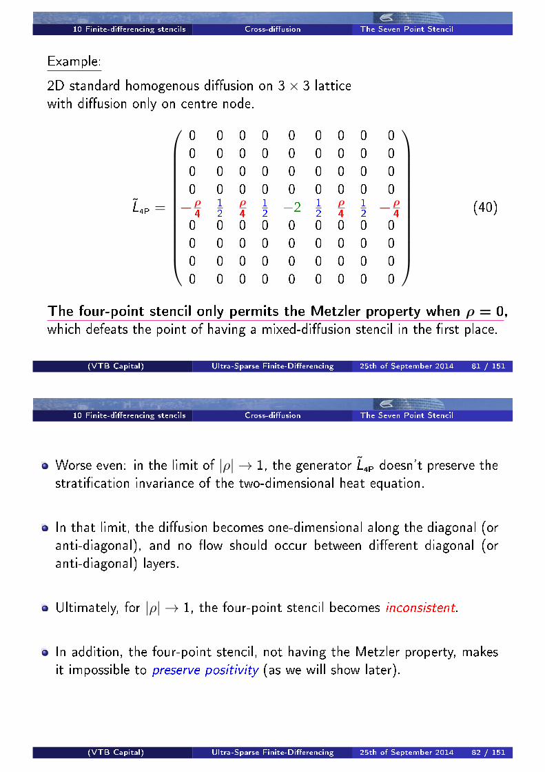
Example:
2D standard homogenous di�usion on 3× 3 latticewith di�usion only on centre node.
L̃4P =
0 0 0 0 0 0 0 0 00 0 0 0 0 0 0 0 00 0 0 0 0 0 0 0 00 0 0 0 0 0 0 0 0−ρ
4
12
ρ4
12−2 1
2ρ4
12−ρ
4
0 0 0 0 0 0 0 0 00 0 0 0 0 0 0 0 00 0 0 0 0 0 0 0 00 0 0 0 0 0 0 0 0
(40)
The four-point stencil only permits the Metzler property when ρ = 0,which defeats the point of having a mixed-di�usion stencil in the �rst place.
(VTB Capital) Ultra-Sparse Finite-Di�erencing 25th of September 2014 81 / 151
10 Finite-di�erencing stencils Cross-di�usion The Seven Point Stencil
Worse even: in the limit of |ρ| → 1, the generator L̃4P doesn't preserve thestrati�cation invariance of the two-dimensional heat equation.
In that limit, the di�usion becomes one-dimensional along the diagonal (oranti-diagonal), and no �ow should occur between di�erent diagonal (oranti-diagonal) layers.
Ultimately, for |ρ| → 1, the four-point stencil becomes inconsistent.
In addition, the four-point stencil, not having the Metzler property, makesit impossible to preserve positivity (as we will show later).
(VTB Capital) Ultra-Sparse Finite-Di�erencing 25th of September 2014 82 / 151
10 Finite-di�erencing stencils The importance of being Metzler
Note: the only non-zero eigenvalue of L̃4P in (40) is actually −2, and thusthere is no �instability� at stake here.
However, in addition to stability, for the later purpose of numerical integra-tion in time to preserve non-negative probabilities, ideally,
we would like at least the fully implicit Padé(0,1) scheme propagator
A(0,1)(L̃) =[1− τ · L̃∗
]−1(41)
over a time step of length τ > 0 to have no negative entries.
(VTB Capital) Ultra-Sparse Finite-Di�erencing 25th of September 2014 83 / 151
10 Finite-di�erencing stencils The importance of being Metzler
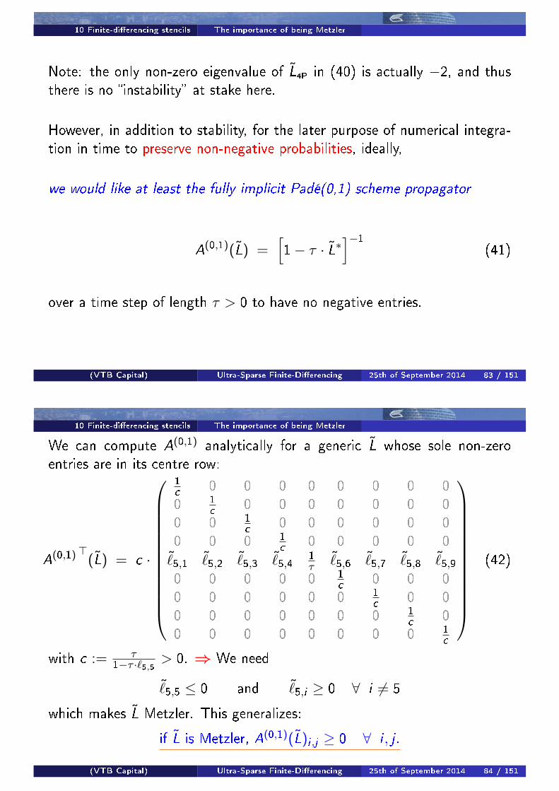
We can compute A(0,1) analytically for a generic L̃ whose sole non-zeroentries are in its centre row:
A(0,1)>(L̃) = c ·
1c 0 0 0 0 0 0 0 00 1
c 0 0 0 0 0 0 00 0 1
c 0 0 0 0 0 00 0 0 1
c 0 0 0 0 0˜̀5,1
˜̀5,2
˜̀5,3
˜̀5,4
1τ
˜̀5,6
˜̀5,7
˜̀5,8
˜̀5,9
0 0 0 0 0 1c 0 0 0
0 0 0 0 0 0 1c 0 0
0 0 0 0 0 0 0 1c 0
0 0 0 0 0 0 0 0 1c
(42)
with c := τ1−τ ·`5,5 > 0. ⇒ We need
˜̀5,5 ≤ 0 and ˜̀
5,i ≥ 0 ∀ i 6= 5
which makes L̃ Metzler. This generalizes:
if L̃ is Metzler, A(0,1)(L̃)i ,j ≥ 0 ∀ i , j .
(VTB Capital) Ultra-Sparse Finite-Di�erencing 25th of September 2014 84 / 151
10 Finite-di�erencing stencils The importance of being Metzler Metzler is su�cient and necessary
In continuous time, we can invoke the generic theorem that
the exponential of a Metzler matrix is a non-negative matrix.
So, L̃ being Metzler is su�cient for eτ ·L̃ to be non-negative.
However, it is straightforward to see from the Taylor expansion
eτ ·L̃ = 1 + τ · L̃ + 1
2τ2 · L̃2 + 1
6τ3 · L̃3 + · · · (43)
that for any non-Metzler L̃, there is some value for τ > 0 for which
(any truncated Taylor expansion of) eτ ·L̃
has negative o�-diagonal elements!
The Metzler property for L̃ is both su�cient and necessary !
Formally, we have (eτ ·L̃)ij ≥ 0 (∀i , j) for all τ ≥ 0 if and only if L̃ is Metzler [Min88].
(VTB Capital) Ultra-Sparse Finite-Di�erencing 25th of September 2014 85 / 151
10 Finite-di�erencing stencils The importance of being Metzler Metzler is su�cient and necessary
To summarize, we want L̃∗ to be Metzler because:-
Ideally, we want whichever numerical scheme we use later for integrationin time to preserve positivity of probabilities.
The only (simple) scheme that (we know of that) can preserve positivity ofp from t to t + τ (for all τ > 0) is the �rst order fully implicit scheme
(1− τ · L̃∗) · p(t + τ) = p(t) (44)
For (44) to preserve positivity (in general, for all τ > 0),
L̃∗ must be Metzler.
Note that we may actually soften up our aim to have strictly positive transitionslater on, and not actually use (44)
but we still aim to preserve the Metzler property with other schemes, too,
since we �nd (heuristically, but de�nitely not suprisingly) that non-positivity ismuch less of an issue when L̃∗ is Metzler.
An example is the �rst order fully explicit scheme which preserves positivity if and only
if L̃∗ is Metzler (and τ is small enough) .
(VTB Capital) Ultra-Sparse Finite-Di�erencing 25th of September 2014 86 / 151

10 Finite-di�erencing stencils Cross-di�usion The Seven Point Stencil
In contrast to the four-point stencil, consider the net generator with theseven-point stencil for the same example (with positive correlation):
L̃7P =
0 0 0 0 0 0 0 0 00 0 0 0 0 0 0 0 00 0 0 0 0 0 0 0 00 0 0 0 0 0 0 0 0
0 1−ρ2
ρ2
1−ρ2
ρ− 2 1−ρ2
ρ2
1−ρ2
00 0 0 0 0 0 0 0 00 0 0 0 0 0 0 0 00 0 0 0 0 0 0 0 00 0 0 0 0 0 0 0 0
(45)
The seven-point stencil preserves the Metzler property for all |ρ| ≤ 1 !
(VTB Capital) Ultra-Sparse Finite-Di�erencing 25th of September 2014 87 / 151
10 Finite-di�erencing stencils Cross-di�usion The Seven Point Stencil
ρ = 1: The central row of L̃7P takes on the form
( 0 0 12
0 −1 0 12
0 0 )
associated node: 1 2 3 4 5 6 7 8 9
as it should: transport only takes place along the anti-diagonal axis.
4P 7P1
4
7
2
5
8
3
6
9
1
4
7
2
5
8
3
6
9
wrong right
(VTB Capital) Ultra-Sparse Finite-Di�erencing 25th of September 2014 88 / 151
10 Finite-di�erencing stencils Cross-di�usion The Seven Point Stencil
The good news is, the seven-point stencil
separates into three uni-directional di�usion components.
For ρ ≥ 0:
∂2
∂z∂yp̃i , j ≈
1
∆z∆y
[pi+1,j+1 − 2pi ,j + pi−1,j−1︸ ︷︷ ︸
zy-component
(46)
− (pi+1,j − 2pi ,j + pi−1,j)︸ ︷︷ ︸z-component
anti-di�usive
− (pi ,j+1 − 2pi ,j + pi ,j−1)︸ ︷︷ ︸y-component
anti-di�usive
]
By combining the
z-component of the mixed-di�usion (seven-point) stencil with the z-di�usiongenerator terms,and the y-component of the mixed-di�usion (seven-point) stencil with they -di�usion generator terms,
we can write the spatially discrete generator as
L̃ = L̃zy + L̃z + L̃y . (47)(VTB Capital) Ultra-Sparse Finite-Di�erencing 25th of September 2014 89 / 151
10 Finite-di�erencing stencils Cross-di�usion The Seven Point Stencil
Notes:
The net operators L̃z and L̃y can have, at this stage,negative local di�usivity.
This will be dealt with later with anti-di�usive �ux limiting.
Equation (47) is in spirit akin to a di�erential operator split.
In practice, we employ a full algebraic split of L̃.
In essence, this means that we really only split the matrix L̃ into three partsafter the boundary conditions have been fully taken into account.
This enables us to minimize the amount of anti-di�usive �ux limiting wehave to impose as part of the de�nition of our spatially discretised model.3
3For more details on the di�erence between di�erential and algebraic operator-splitting, Algebraic Flux Corrections (AFC), and Flux Corrected Transport (FCT)see, e.g., [Kuz07, Kuz10, BLOG93].
(VTB Capital) Ultra-Sparse Finite-Di�erencing 25th of September 2014 90 / 151

11 Boundary Conditions
Common �wisdom� has it that:-
boundary conditions matter little,
the boundary always has to be moved out a long way,
one always needs a lot of nodes,
�if the boundary conditions seem to a�ect your result, the boundary needsto be moved out further, and you need to use more nodes�.
(VTB Capital) Ultra-Sparse Finite-Di�erencing 25th of September 2014 91 / 151
11 Boundary Conditions
There is a large volume of literature in engineering and Computational FluidDynamics dedicated to boundary conditions. They do matter.
Our design here is to be ultra-sparse, e.g., typically, 25× 11 nodes.
With very few nodes, the boundaries (by mere node-count-proximity) alwayshave a signi�cant in�uence on the central region.
Real physical spatially discrete (model) systems with few nodes behaveperfectly reasonably, so why shouldn't our model equations?(recall that our equations are discrete in space but continuous in time, and thus can
still be represented by an actual physical experiment)
On sparse lattices, the boundary nodes make up a signi�cant percentage:
Discretisation Total nodes Boundary nodes Percentage
15× 5 75 36 48% ≈ 1/221× 7 147 52 35.4% ≈ 1/325× 11 275 68 24.7% ≈ 1/4
We should make full use of the boundary nodes for the sake of e�ciency!
(VTB Capital) Ultra-Sparse Finite-Di�erencing 25th of September 2014 92 / 151
11 Boundary Conditions Martingale requirements
In support of the intended algebraic split
L̃ = L̃z + L̃y + L̃zy (47)
we choose boundary conditions directly for L̃z , L̃y , and L̃zy according to:-
The generator must be an x-martingale.
This means that x- (and thus z-) direction boundary nodes must have no(outoging) transport in the x- (and thus z-) direction.Absorption.
By the same token, zy -direction boundary nodes must have no (outoging)transport in the zy -direction.Absorption.
In contrast, y -direction boundary nodes have no y -martingale requirements:transport is permissible in and out in the y -direction.Re�ection.
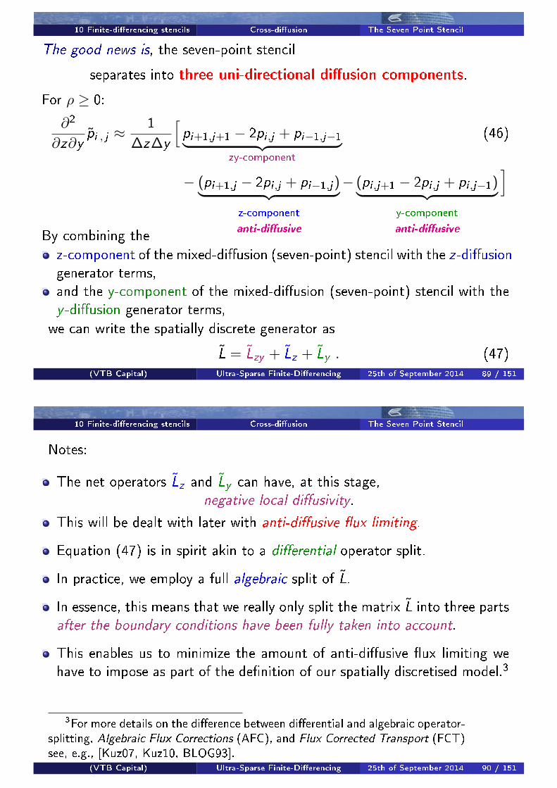
(VTB Capital) Ultra-Sparse Finite-Di�erencing 25th of September 2014 93 / 151
11 Boundary Conditions Permissible transport
Permissible Transport:
ρ < 0
z
y
(VTB Capital) Ultra-Sparse Finite-Di�erencing 25th of September 2014 94 / 151
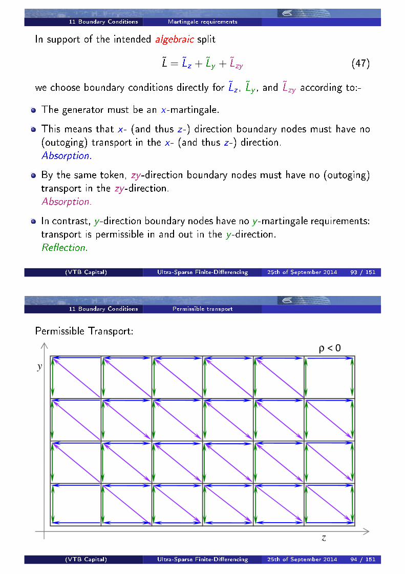
11 Boundary Conditions Permissible transport L̃z absorption points
L̃z absorption points:
ρ < 0
z
y
(VTB Capital) Ultra-Sparse Finite-Di�erencing 25th of September 2014 95 / 151
11 Boundary Conditions Permissible transport L̃zy absorption points
L̃zy absorption points:
ρ < 0
z
y
(VTB Capital) Ultra-Sparse Finite-Di�erencing 25th of September 2014 96 / 151
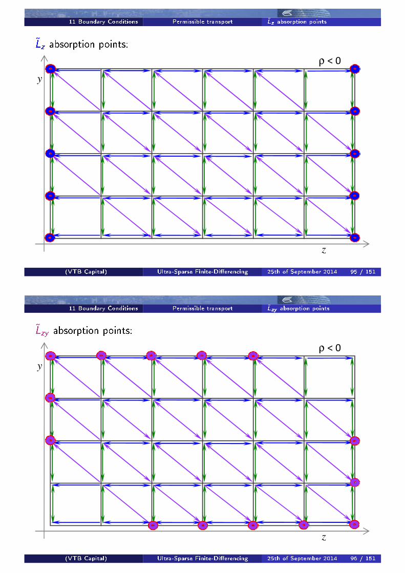
11 Boundary Conditions Permissible transport L̃y re�ection points
L̃y re�ection points:
ρ < 0
z
y
(VTB Capital) Ultra-Sparse Finite-Di�erencing 25th of September 2014 97 / 151
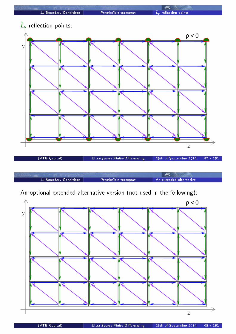
11 Boundary Conditions Permissible transport An extended alternative
An optional extended alternative version (not used in the following):
ρ < 0
z
y
(VTB Capital) Ultra-Sparse Finite-Di�erencing 25th of September 2014 98 / 151
11 Boundary Conditions Absortion and Re�ection
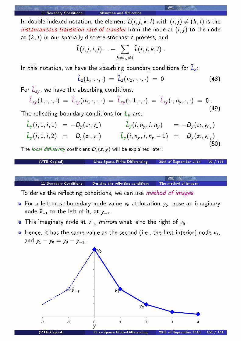
In double-indexed notation, the element L̃(i , j , k , l) with (i , j) 6= (k , l) is theinstantaneous transition rate of transfer from the node at (i , j) to the nodeat (k , l) in our spatially discrete stochastic process, and
L̃(i , j , i , j) = −∑
k 6=i ,j 6=l
L̃(i , j , k , l) .
In this notation, we have the absorbing boundary conditions for L̃z :
L̃z(1, ·, ·, ·) = L̃z(nz , ·, ·, ·) = 0 (48)
For L̃zy , we have the absorbing conditions:
L̃zy (1, ·, ·, ·) = L̃zy (nz , ·, ·, ·) = L̃zy (·, 1, ·, ·) = L̃zy (·, ny , ·, ·) = 0 .(49)
The re�ecting boundary conditions for Ly are:
L̃y (i , 1, i , 1) = −Dy (zi , y1) L̃y (i , ny , i , ny ) = −Dy (zi , yny )
L̃y (i , 1, i , 2) = Dy (zi , y1) L̃y (i , ny , i , ny − 1) = Dy (zi , yny )(50)
The local di�usivity coe�cient Dy (z , y) will be explained later.
(VTB Capital) Ultra-Sparse Finite-Di�erencing 25th of September 2014 99 / 151
11 Boundary Conditions Deriving the re�ecting conditions The method of images
To derive the re�ecting conditions, we can use method of images.
For a left-most boundary node value v0 at location y0, pose an imaginarynode v̆−1 to the left of it, at y−1.
This imaginary node at y−1 mirrors what is to the right of y0.
Hence, it has the same value as the second (i.e., the �rst interior) node v1,and y1 − y0 = y0 − y−1.
-2 -1 0 1 2 3 4
y
v̆−1
v0
v1
v2
(VTB Capital) Ultra-Sparse Finite-Di�erencing 25th of September 2014 100 / 151
11 Boundary Conditions Deriving the re�ecting conditions The method of images
This gives us for the �rst derivative with standard centre-di�erencing
∂v
∂y
∣∣∣∣y=y0
≈ v1 − v̆−12∆y
(51)
=v1 − v12∆y
= 0
=⇒ The re�ecting boundary condition means NO ADVECTION!
(VTB Capital) Ultra-Sparse Finite-Di�erencing 25th of September 2014 101 / 151
11 Boundary Conditions Deriving the re�ecting conditions The method of images
For the di�usion term, we obtain from the method of images that the totallocal di�usion �ux is proportional to
∂2v
∂y2
∣∣∣∣y=y0
≈ v1 − 2v0 + v̆−1∆y2
(52)
=v1 − 2v0 + v1
∆y2
= 2 · v1 − v0∆y2
.
This, however, includes the �ux to and from the imaginary node!
By symmetry, only half of this is actual �ux to and from the interior node,and hence no factor 2 in (50).
=⇒The re�ecting boundary condition makes a di�usion term look like aone-sided, i.e., forward-di�erencing, advection term.
(VTB Capital) Ultra-Sparse Finite-Di�erencing 25th of September 2014 102 / 151
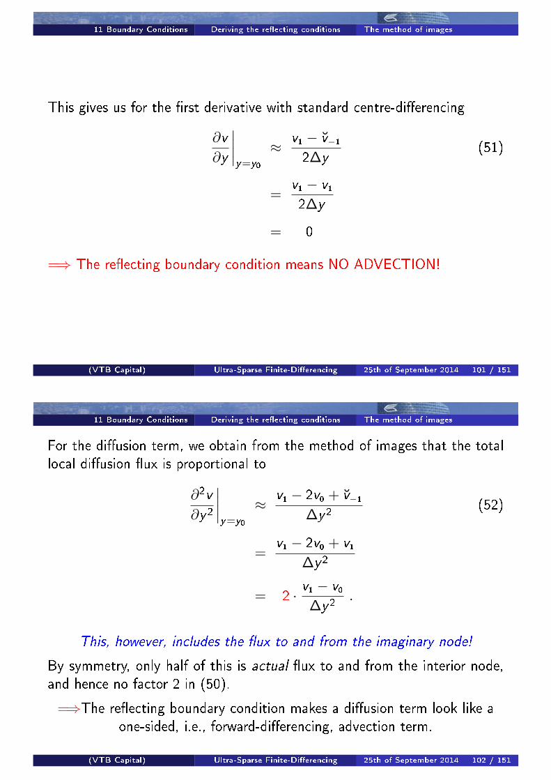
11 Boundary Conditions Deriving the re�ecting conditions From continuous equations
We note that conventional (spatially continuous) notation for a re�ecting boundarycondition is
∂v
∂y= 0. (53)
In a spatially discretised form, this forces the advection term to be 0.
The di�usion term can be realized by extending the domain by an additional (non-imaginary) node at y−1 (though this can in principle be asymmetric, i.e., closer toy0):
-2 -1 0 1 2 3 4
y
v−1
v0
v1
v2
(VTB Capital) Ultra-Sparse Finite-Di�erencing 25th of September 2014 103 / 151
11 Boundary Conditions Deriving the re�ecting conditions From continuous equations
Using forward di�erencing for advection terms in this extra node, the condi-tion
0 =∂v
∂y
∣∣∣∣y=y−1
≈ v0 − v−1∆y
(54)
enforces the identityv−1 ≡ v0 . (55)
This gives us for the di�usion term in y0
∂2v
∂y2
∣∣∣∣y=y0
≈ v1 − 2v0 + v−1∆y2
=v1 − 2v0 + v0
∆y2=
v1 − v0∆y2
(56)
which is exactly what we had from the spatially discretised method of images.
This derivation here is based on the spatially continuous re�ection con-dition (53) results in the same dynamics on the interior and the boundarynode in y0. The only di�erence is the extra auxiliary node at y−1 which is ofno dynamic value or modelling contribution. It is literally a waste of space.
(VTB Capital) Ultra-Sparse Finite-Di�erencing 25th of September 2014 104 / 151

12 Ensuring continuous-time stability Local di�usivity in continuous time
The three components of L̃ = L̃z + L̃y + L̃zy are:-
L̃z : advection-di�usion generator with local di�usivity
Dz(z , y) = 12
(ς(z,y)2
∆z2− |ρ|ς(z,y)α
√2κ
∆z∆y
)(57)
L̃y : advection-di�usion generator with local di�usivity
Dy (z , y) = 12
(2κα2
∆y2− |ρ|ς(z,y)α
√2κ
∆z∆y
)(58)
L̃zy : pure di�usion generator with local di�usivity
Dzy (z , y) = 12|ρ|ς(z,y)α
√2κ
∆z∆y (59)
withς(z , y) := σ0 e
−z f (ez)g(y) . (21)
(VTB Capital) Ultra-Sparse Finite-Di�erencing 25th of September 2014 105 / 151
12 Ensuring continuous-time stability Local di�usivity in continuous time
Why the special attention on the di�usion part?
A pure advection term can give rise to oscillatory modes, butnot to growing modes.
The sign of the advection coe�cient can be either way � it has no impacton mode stability.
A physical di�usion term has eigenvalues with non-positive real parts. Realworld di�usion does not concentrate distributions, it di�uses them.The clue is in the name.
A di�usion term is physical if its local di�usivity is non-negative.
A di�usion term with negative local di�usivity causes exponentially growingmodes. It violates the Maximum Principle.
A growing (localized) mode can be caused by any local di�usivity of anyof the three of L̃z , L̃y , and L̃zy to be negative anywhere.
In order to ensure continuous-time stability, we demand that alllocal di�usivities are non-negative everywhere.
(VTB Capital) Ultra-Sparse Finite-Di�erencing 25th of September 2014 106 / 151
12 Ensuring continuous-time stability Local di�usivity in continuous time Anti-di�usive �ux limiting
For any given value of |ρ|, either Dz or Dy can be negative, but not both.
To see this, de�neR(z , y) := ς(z,y)
α√2κ
∆y∆z , (60)
then
Dz(z , y) = 12ς(z,y)α
√2κ
∆z∆y
(R(z , y)− |ρ|
)(61)
Dy (z , y) = 12ς(z,y)α
√2κ
∆z∆y
(1
R(z,y) − |ρ|). (62)
Since R(z , y) ≥ 0, both of Dz(z , y) and Dy (z , y) are non-negative when
|ρ| ≤ min
(R(z , y),
1
R(z , y)
). (63)
(VTB Capital) Ultra-Sparse Finite-Di�erencing 25th of September 2014 107 / 151
12 Ensuring continuous-time stability Local di�usivity in continuous time Anti-di�usive �ux limiting
However, when
|ρ| > |ρ|max (64)with
|ρ|max := minz,y
(R(z , y),
1
R(z , y)
), (65)
then some of the local di�usivities Dz(z , y) and Dy (z , y) on the lattice arenegative, which is not admissible.
When this happens, we �oor the respective local di�usivity at zero.
This is called Anti-Di�usive Flux Limiting.
Note that only one of Dz(z , y) and Dy (z , y) can be negative at any one node.
We emphasize that this �ooring of coe�cients does not constitute an inconsistency with
our model choice because our model choice is the net result of discretisation, after all
adjustments, in the form of the �nal (spatially discrete) generator L̃.
(VTB Capital) Ultra-Sparse Finite-Di�erencing 25th of September 2014 108 / 151
12 Ensuring continuous-time stability Local di�usivity in continuous time How bad could it possibly be?
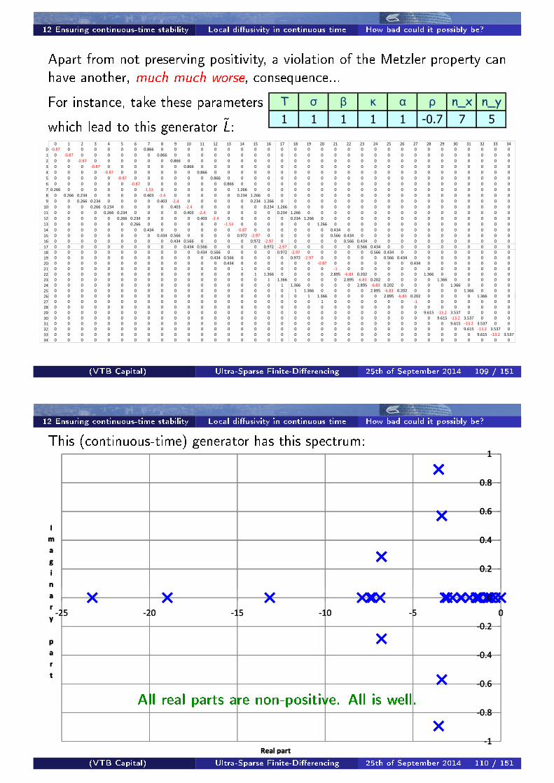
Apart from not preserving positivity, a violation of the Metzler property canhave another, much much worse, consequence...
For instance, take these parameters � � � � � � ��� ���
� � � � � ���� � �which lead to this generator L̃:
� � � � � � � � � �� �� �� �� �� �� �� �� �� � �� �� �� �� �� �� �� �� �� � �� �� �� �� ��
� ���� � � � � � � ����� � � � � � � � � � � � � � � � � � � � � � � � � � � �
� � ���� � � � � � � ����� � � � � � � � � � � � � � � � � � � � � � � � � � �
� � � ���� � � � � � � ����� � � � � � � � � � � � � � � � � � � � � � � � � �
� � � � ���� � � � � � � ����� � � � � � � � � � � � � � � � � � � � � � � � �
� � � � � ���� � � � � � � ����� � � � � � � � � � � � � � � � � � � � � � � �
� � � � � � ���� � � � � � � ����� � � � � � � � � � � � � � � � � � � � � � �
� � � � � � � ���� � � � � � � ����� � � � � � � � � � � � � � � � � � � � � �
� ����� � � � � � � ���� � � � � � � ����� � � � � � � � � � � � � � � � � � � � �
� � ����� ����� � � � � ����� ��� � � � � � ����� ����� � � � � � � � � � � � � � � � � � � �
� � ����� ����� � � � � ����� ��� � � � � � ����� ����� � � � � � � � � � � � � � � � � � �
�� � � � ����� ����� � � � � ����� ��� � � � � � ����� ����� � � � � � � � � � � � � � � � � �
�� � � � � ����� ����� � � � � ����� ��� � � � � � ����� ����� � � � � � � � � � � � � � � � �
�� � � � � � ����� ����� � � � � ����� ��� � � � � � ����� ����� � � � � � � � � � � � � � � �
�� � � � � � � ����� � � � � � � ���� � � � � � � ����� � � � � � � � � � � � � � �
�� � � � � � � � ����� � � � � � � ���� � � � � � � ����� � � � � � � � � � � � � �
�� � � � � � � � � ����� ����� � � � � ���� ��� � � � � � ����� ����� � � � � � � � � � � � �
�� � � � � � � � � � ����� ����� � � � � ���� ��� � � � � � ����� ����� � � � � � � � � � � �
�� � � � � � � � � � � ����� ����� � � � � ���� ��� � � � � � ����� ����� � � � � � � � � � �
�� � � � � � � � � � � � ����� ����� � � � � ���� ��� � � � � � ����� ����� � � � � � � � � �
� � � � � � � � � � � � � ����� ����� � � � � ���� ��� � � � � � ����� ����� � � � � � � � �
�� � � � � � � � � � � � � � ����� � � � � � � ���� � � � � � � ����� � � � � � � �
�� � � � � � � � � � � � � � � � � � � � � � � � � � � � � � � � � � � �
�� � � � � � � � � � � � � � � � � ����� � � � � ���� ���� ����� � � � � ����� � � � � � �
�� � � � � � � � � � � � � � � � � � ����� � � � � ���� ���� ����� � � � � ����� � � � � �
�� � � � � � � � � � � � � � � � � � � ����� � � � � ���� ���� ����� � � � � ����� � � � �
�� � � � � � � � � � � � � � � � � � � � ����� � � � � ���� ���� ����� � � � � ����� � � �
�� � � � � � � � � � � � � � � � � � � � � ����� � � � � ���� ���� ����� � � � � ����� � ��� � � � � � � � � � � � � � � � � � � � � ����� � � � � ���� ���� ����� � � � � ����� � �
�� � � � � � � � � � � � � � � � � � � � � � � � � � � � � � � � � � � �
�� � � � � � � � � � � � � � � � � � � � � � � � � � � � � � � � � � � �
� � � � � � � � � � � � � � � � � � � � � � � � � � � � � ���� ���� ����� � � � �
�� � � � � � � � � � � � � � � � � � � � � � � � � � � � � � ���� ���� ����� � � �
�� � � � � � � � � � � � � � � � � � � � � � � � � � � � � � � ���� ���� ����� � �
�� � � � � � � � � � � � � � � � � � � � � � � � � � � � � � � � ���� ���� ����� �
�� � � � � � � � � � � � � � � � � � � � � � � � � � � � � � � � � ���� ���� �����
�� � � � � � � � � � � � � � � � � � � � � � � � � � � � � � � � � � � �
(VTB Capital) Ultra-Sparse Finite-Di�erencing 25th of September 2014 109 / 151
12 Ensuring continuous-time stability Local di�usivity in continuous time How bad could it possibly be?
This (continuous-time) generator has this spectrum:
�
���
���
���
���
�
�
�
�
�
�
�
�
�
�
�
�
�
��
����
����
����
����
�
���
���
���
���
�
��� ��� ��� ��� �� �
�
�
�
�
�
�
�
�
�
�
�
�
��� ���
��
����
����
����
����
�
���
���
���
���
�
��� ��� ��� ��� �� �
�
�
�
�
�
�
�
�
�
�
�
�
��� ���
All real parts are non-positive. All is well.
(VTB Capital) Ultra-Sparse Finite-Di�erencing 25th of September 2014 110 / 151
12 Ensuring continuous-time stability Local di�usivity in continuous time How bad could it possibly be?
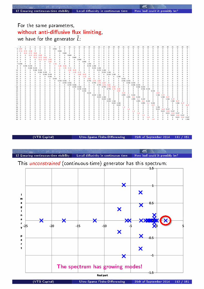
For the same parameters,without anti-di�usive �ux limiting,we have for the generator L̃:
� � � � � � � � � �� �� �� �� �� �� �� �� �� � �� �� �� �� �� �� �� �� �� � �� �� �� �� ��
� ���� � � � � � � ����� � � � � � � � � � � � � � � � � � � � � � � � � � � �
� ���� ���� ���� � � � � � ����� � � � � � � � � � � � � � � � � � � � � � � � � � �
� � ���� ���� ���� � � � � � ����� � � � � � � � � � � � � � � � � � � � � � � � � �
� � � ���� ���� ���� � � � � � ����� � � � � � � � � � � � � � � � � � � � � � � � �
� � � � ���� ���� ���� � � � � � ����� � � � � � � � � � � � � � � � � � � � � � � �
� � � � � ���� ���� ���� � � � � � ����� � � � � � � � � � � � � � � � � � � � � � �
� � � � � � � ���� � � � � � � ����� � � � � � � � � � � � � � � � � � � � � �
� ����� � � � � � � ���� � � � � � � ����� � � � � � � � � � � � � � � � � � � � �
� � ����� ����� � � � � � ���� ���� � � � � ����� ����� � � � � � � � � � � � � � � � � � � �
� � ����� ����� � � � � � ���� ���� � � � � ����� ����� � � � � � � � � � � � � � � � � � �
�� � � � ����� ����� � � � � � ���� ���� � � � � ����� ����� � � � � � � � � � � � � � � � � �
�� � � � � ����� ����� � � � � � ���� ���� � � � � ����� ����� � � � � � � � � � � � � � � � �
�� � � � � � ����� ����� � � � � � ���� ���� � � � � ����� ����� � � � � � � � � � � � � � � �
�� � � � � � � ����� � � � � � � ���� � � � � � � ����� � � � � � � � � � � � � � �
�� � � � � � � � ����� � � � � � � ���� � � � � � � ����� � � � � � � � � � � � � �
�� � � � � � � � � ����� ����� � � � � ���� ���� ���� � � � � ����� ����� � � � � � � � � � � � �
�� � � � � � � � � � ����� ����� � � � � ���� ���� ���� � � � � ����� ����� � � � � � � � � � � �
�� � � � � � � � � � � ����� ����� � � � � ���� ���� ���� � � � � ����� ����� � � � � � � � � � �
�� � � � � � � � � � � � ����� ����� � � � � ���� ���� ���� � � � � ����� ����� � � � � � � � � �
� � � � � � � � � � � � � ����� ����� � � � � ���� ���� ���� � � � � ����� ����� � � � � � � � �
�� � � � � � � � � � � � � � ����� � � � � � � ���� � � � � � � ����� � � � � � � �
�� � � � � � � � � � � � � � � ����� � � � � � � ���� � � � � � � ���� � � � � � �
�� � � � � � � � � � � � � � � � ����� ����� � � � � ���� ��� ����� � � � � ����� ���� � � � � �
�� � � � � � � � � � � � � � � � � ����� ����� � � � � ���� ��� ����� � � � � ����� ���� � � � �
�� � � � � � � � � � � � � � � � � � ����� ����� � � � � ���� ��� ����� � � � � ����� ���� � � �
�� � � � � � � � � � � � � � � � � � � ����� ����� � � � � ���� ��� ����� � � � � ����� ���� � �
�� � � � � � � � � � � � � � � � � � � � ����� ����� � � � � ���� ��� ����� � � � � ����� ���� ��� � � � � � � � � � � � � � � � � � � � ����� ����� � � � � ���� ��� ����� � � � � ����� ���� �
�� � � � � � � � � � � � � � � � � � � � � ����� � � � � � � ���� � � � � � � ����
�� � � � � � � � � � � � � � � � � � � � � � ��� � � � � � � ���� � � � � � �
� � � � � � � � � � � � � � � � � � � � � � � ��� � � � � � ���� ���� ����� � � � �
�� � � � � � � � � � � � � � � � � � � � � � � � ��� � � � � � ���� ���� ����� � � �
�� � � � � � � � � � � � � � � � � � � � � � � � � ��� � � � � � ���� ���� ����� � �
�� � � � � � � � � � � � � � � � � � � � � � � � � � ��� � � � � � ���� ���� ����� �
�� � � � � � � � � � � � � � � � � � � � � � � � � � � ��� � � � � � ���� ���� �����
�� � � � � � � � � � � � � � � � � � � � � � � � � � � � ��� � � � � � � ����
(VTB Capital) Ultra-Sparse Finite-Di�erencing 25th of September 2014 111 / 151
12 Ensuring continuous-time stability Local di�usivity in continuous time How bad could it possibly be?
This unconstrained (continuous-time) generator has this spectrum:
���
�
���
�
�
�
�
�
�
�
�
�
�
�
�
����
��
����
�
���
�
���
��� ��� ��� ��� �� � �
�
�
�
�
�
�
�
�
�
�
�
�
��� �������
��
����
�
���
�
���
��� ��� ��� ��� �� � �
�
�
�
�
�
�
�
�
�
�
�
�
��� ���
The spectrum has growing modes!
(VTB Capital) Ultra-Sparse Finite-Di�erencing 25th of September 2014 112 / 151
12 Ensuring continuous-time stability Local di�usivity in continuous time How bad could it possibly be?
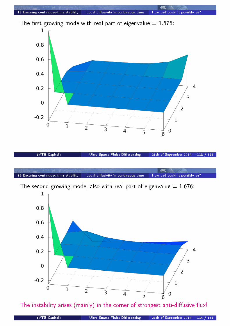
The �rst growing mode with real part of eigenvalue = 1.676:
0 1 2 3 4 5 6 0
1
2
3
4
-0.2
0
0.2
0.4
0.6
0.8
1
(VTB Capital) Ultra-Sparse Finite-Di�erencing 25th of September 2014 113 / 151
12 Ensuring continuous-time stability Local di�usivity in continuous time How bad could it possibly be?
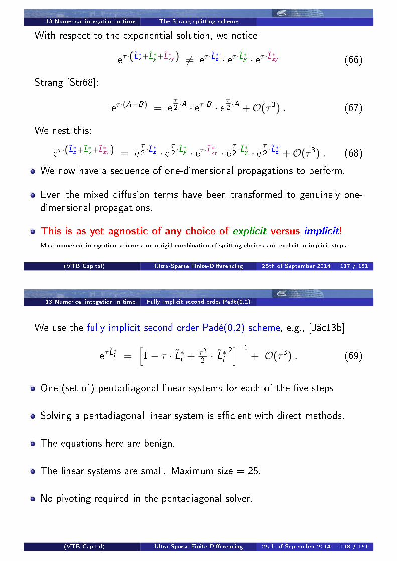
The second growing mode, also with real part of eigenvalue = 1.676:
0 1 2 3 4 5 6 0
1
2
3
4
-0.2
0
0.2
0.4
0.6
0.8
1
The instability arises (mainly) in the corner of strongest anti-di�usive �ux!
(VTB Capital) Ultra-Sparse Finite-Di�erencing 25th of September 2014 114 / 151

12 Ensuring continuous-time stability Local di�usivity in continuous time How bad could it possibly be?
Note that these instabilities are not to be confused with those arising fromschemes for numerical integration in time.Those, typically, (as for the �rst order explicit scheme), are associated withthe mode of the most negative eigenvalue (here, about -22):
0 1 2 3 4 5 6 0
1
2
3
4
-0.2
0
0.2
0.4
0.6
0.8
1
(VTB Capital) Ultra-Sparse Finite-Di�erencing 25th of September 2014 115 / 151
13 Numerical integation in time Actual continuous time
Recall that the spatially discrete dynamic equations
∂∂t p̃ = L̃∗ · p̃ (22)
have the continuous-time solution
p̃(t + τ) = eτ ·L̃∗· p̃(t) . (23)
In principle, this can be evaluated directly by the aid of a numerical routinefor the computation of the exponential of τ · L̃∗.
Much more e�ciently, one would use a method that gives the result of theaction of eτ ·L̃
∗on a given vector p̃.
E.g., R. Sidje's ExpoKit [Sid98] which combines a Krylov-Arnoldi projection to reduce the dimensionality combined
with a 12-th order (!) Padé(6,6) approximation to the exponential of the reduced linear system (which is much smaller
than the original linear system). ExpoKit also automatically inserts sub-steps based on a formal error analysis.
For production purposes, we can do something faster.
(VTB Capital) Ultra-Sparse Finite-Di�erencing 25th of September 2014 116 / 151
13 Numerical integation in time The Strang splitting scheme
With respect to the exponential solution, we notice
eτ ·(L̃∗z+L̃∗y+L̃∗zy) 6= e
τ ·L̃∗z · eτ ·L̃∗y · eτ ·L̃∗zy (66)
Strang [Str68]:
eτ ·(A+B) = e
τ2·A · eτ ·B · e
τ2·A +O(τ3) . (67)
We nest this:
eτ ·(L̃∗z+L̃∗y+L̃∗zy) = e
τ2·L̃∗z · e
τ2·L̃∗y · eτ ·L̃∗zy · e
τ2·L̃∗y · e
τ2·L̃∗z +O(τ3) . (68)
We now have a sequence of one-dimensional propagations to perform.
Even the mixed di�usion terms have been transformed to genuinely one-dimensional propagations.
This is as yet agnostic of any choice of explicit versus implicit!Most numerical integration schemes are a rigid combination of splitting choices and explicit or implicit steps.
(VTB Capital) Ultra-Sparse Finite-Di�erencing 25th of September 2014 117 / 151
13 Numerical integation in time Fully implicit second order Padé(0,2)
We use the fully implicit second order Padé(0,2) scheme, e.g., [Jäc13b]
eτ L̃∗i =
[1− τ · L̃∗i + τ2
2· L̃∗i
2]−1
+ O(τ3) . (69)
One (set of) pentadiagonal linear systems for each of the �ve steps
Solving a pentadiagonal linear system is e�cient with direct methods.
The equations here are benign.
The linear systems are small. Maximum size = 25.
No pivoting required in the pentadiagonal solver.
(VTB Capital) Ultra-Sparse Finite-Di�erencing 25th of September 2014 118 / 151
13 Numerical integation in time Remark on alternative schemes
Other schemes are available, e.g., Craig-Sneyd [CS88], Modi�ed Craig-Sneyd [itHM10], Hundsdorfer-Verwer [itHW09, HV03],
or, when combined with the Strang splitting method, Crank-Nicolson scheme [CN47],Lawson-Morris [LM78], etc.
All of these schemes have explicit components.
Explicit components forego positivity preservation.
We propagate Green's functions, i.e., probabilities:we cannot a�ord having any negative p̃z marginals
since that would result in arbitrageable vanilla option prices.
With all of the L̃i being Metzler, the �rst order fully implicit scheme per-fectly preserves positivity.
The second order fully implicity scheme is not perfect, but much betterthan any of the alternatives, and of second order (!)
As long as we take 5 steps to the �rst observation horizon, we found wealways have non-negative probabilities with Padé(0,2).
(VTB Capital) Ultra-Sparse Finite-Di�erencing 25th of September 2014 119 / 151
13 Numerical integation in time Fine correction of the forward
In continuous time, our generator L̃∗ was a perfect x-martingale operator.
With a numerical integration scheme, we incur a small error of order τ3.
At every target horizon, all we want is an implied volatility interpolator fromthe option prices computed from the discrete probabilities.
We correct for the (very small) drift error by a numerical rescaling of theinterpolator strike levels by the e�ective numerical forward.
We interpolate implied volatilities with the arbitrage-free interpolation methoddiscussed in [Jäc13a].
The net result is a spatially continuous implied volatility pro�le at the targethorizon that has no drift error whatsoever.
No arbitrage, no drift error on the forward, everybody wins.
(VTB Capital) Ultra-Sparse Finite-Di�erencing 25th of September 2014 120 / 151
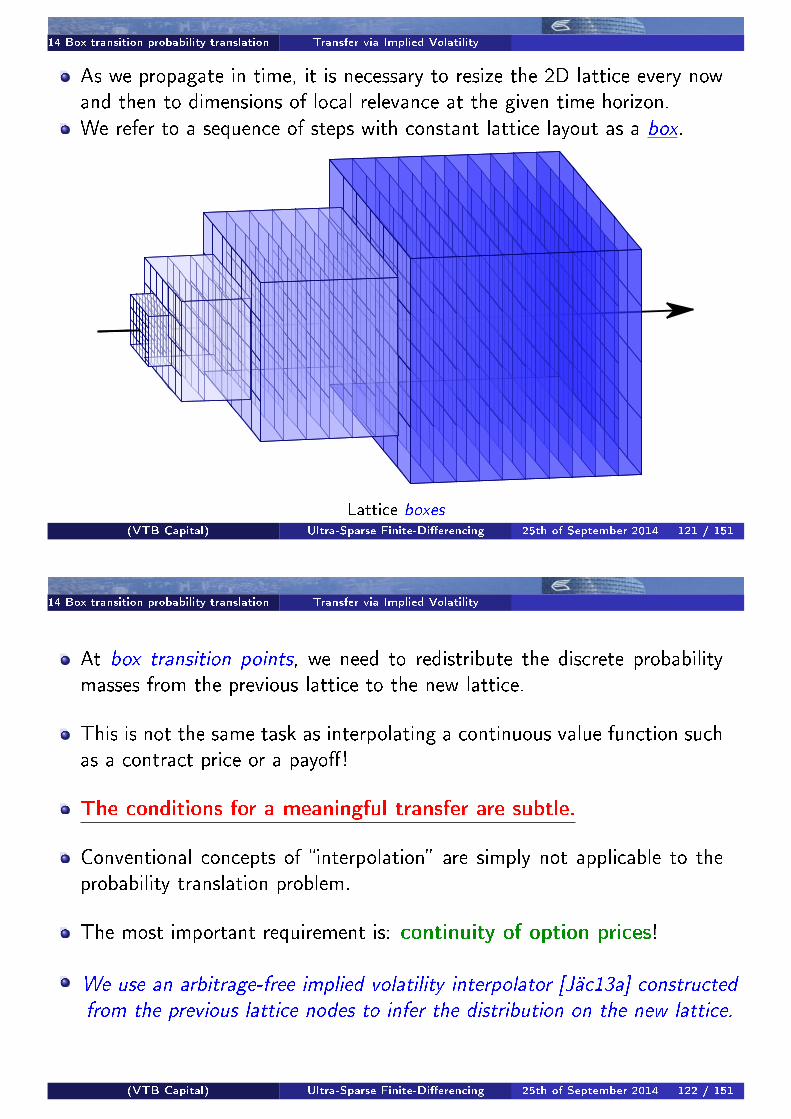
14 Box transition probability translation Transfer via Implied Volatility
As we propagate in time, it is necessary to resize the 2D lattice every nowand then to dimensions of local relevance at the given time horizon.
We refer to a sequence of steps with constant lattice layout as a box.
Lattice boxes(VTB Capital) Ultra-Sparse Finite-Di�erencing 25th of September 2014 121 / 151
14 Box transition probability translation Transfer via Implied Volatility
At box transition points, we need to redistribute the discrete probabilitymasses from the previous lattice to the new lattice.
This is not the same task as interpolating a continuous value function suchas a contract price or a payo�!
The conditions for a meaningful transfer are subtle.
Conventional concepts of �interpolation� are simply not applicable to theprobability translation problem.
The most important requirement is: continuity of option prices!
We use an arbitrage-free implied volatility interpolator [Jäc13a] constructedfrom the previous lattice nodes to infer the distribution on the new lattice.
(VTB Capital) Ultra-Sparse Finite-Di�erencing 25th of September 2014 122 / 151
14 Box transition probability translation Transfer via Implied Volatility From prices back to probabilities
First, we compute out-of-the money option prices {vi}, i = 1...nz , struckat the new lattice's spot levels.
Dropping the leftmost and rightmost nodes, we bootstrap a set of discretez-marginal probabilities p̃′(z ′i ) such that
v ′k =imin(ez
′k )∑
i=1
p̃′(z ′i ) · (ez′k − e
z ′i ) for 1 < k < nz+12
v ′k =nz∑
i=imin(ez′k )
p̃′(z ′i ) · (ez′i − e
z ′k ) for nz+1
2< k < nz
p̃′(z ′nz+12
) = 1−∑
i 6= nz+12
p̃′(z ′i )
(70)
where we have assumed that nz is odd and greater than four.
(VTB Capital) Ultra-Sparse Finite-Di�erencing 25th of September 2014 123 / 151
14 Box transition probability translation Transfer via Implied Volatility From prices back to probabilities
We then redistribute p′i in the y direction by building a two-dimensionalinterpolator Q(z , y) of discrete probabilities from p̃(zi , yj), i.e., from thedata of the earlier box's lattice.
We use this two-dimensional interpolator for the purpose of interpolationin the y -direction, conditional on a given z-level, and so to distribute thez-marginal probability mass at some level zi in the y -direction.
After �ooring and conditioning, the discrete Green's function on the newlattice is given by
p̃(z ′i , y′j ) = p̃′(zi ) ·
(Q(z ′i , y
′j ))
+∑l
(Q(z ′i , y
′l ))
+
. (71)
(VTB Capital) Ultra-Sparse Finite-Di�erencing 25th of September 2014 124 / 151
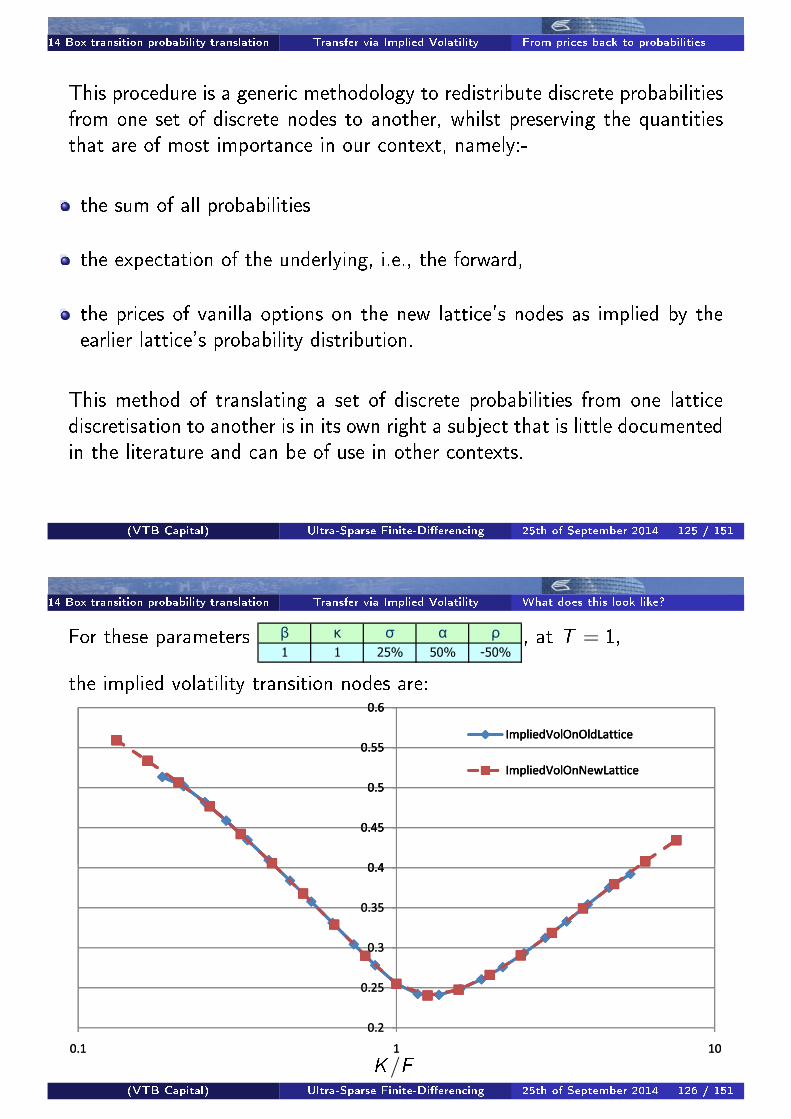
14 Box transition probability translation Transfer via Implied Volatility From prices back to probabilities
This procedure is a generic methodology to redistribute discrete probabilitiesfrom one set of discrete nodes to another, whilst preserving the quantitiesthat are of most importance in our context, namely:-
the sum of all probabilities
the expectation of the underlying, i.e., the forward,
the prices of vanilla options on the new lattice's nodes as implied by theearlier lattice's probability distribution.
This method of translating a set of discrete probabilities from one latticediscretisation to another is in its own right a subject that is little documentedin the literature and can be of use in other contexts.
(VTB Capital) Ultra-Sparse Finite-Di�erencing 25th of September 2014 125 / 151
14 Box transition probability translation Transfer via Implied Volatility What does this look like?
For these parameters � � � � �
� � ��� ��� ����
, at T = 1,
the implied volatility transition nodes are:
���
����
���
����
���
������ �����������
������ ����������
���
����
���
����
���
����
���
����
���
��� � ��
������ �����������
������ ����������
���
����
���
����
���
����
���
����
���
��� � ��
������ �����������
������ ����������
K/F(VTB Capital) Ultra-Sparse Finite-Di�erencing 25th of September 2014 126 / 151
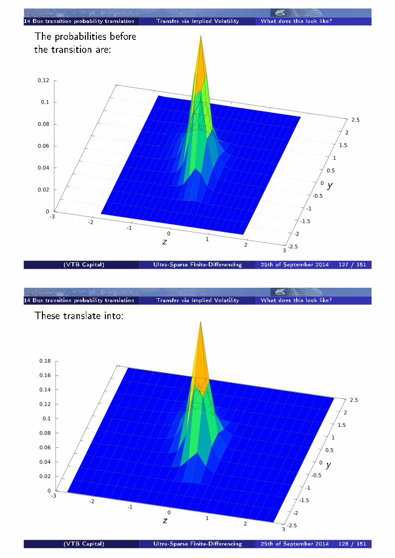
14 Box transition probability translation Transfer via Implied Volatility What does this look like?
The probabilities beforethe transition are:
-2.5
-2
-1.5
-1
-0.5
0
0.5
1
1.5
2
2.5
-3-2
-1 0
1 2
3
0
0.02
0.04
0.06
0.08
0.1
0.12
z
y
(VTB Capital) Ultra-Sparse Finite-Di�erencing 25th of September 2014 127 / 151
14 Box transition probability translation Transfer via Implied Volatility What does this look like?
These translate into:
-2.5
-2
-1.5
-1
-0.5
0
0.5
1
1.5
2
2.5
-3-2
-1 0
1 2
3
0
0.02
0.04
0.06
0.08
0.1
0.12
0.14
0.16
0.18
z
y
(VTB Capital) Ultra-Sparse Finite-Di�erencing 25th of September 2014 128 / 151
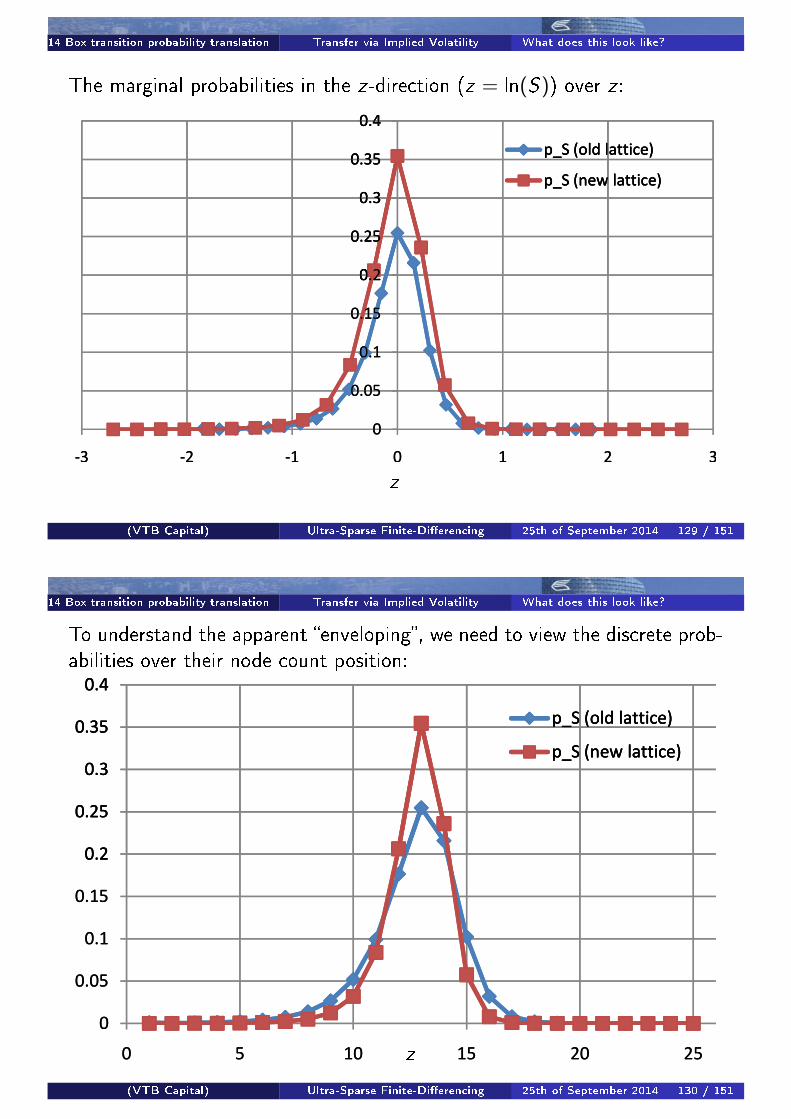
14 Box transition probability translation Transfer via Implied Volatility What does this look like?
The marginal probabilities in the z-direction (z = ln(S)) over z :
���
����
���
����
���
����� ��������
��������������
�
����
���
����
���
����
���
����
���
�� �� �� � � � �
����� ��������
��������������
�
����
���
����
���
����
���
����
���
�� �� �� � � � �
����� ��������
��������������
z
(VTB Capital) Ultra-Sparse Finite-Di�erencing 25th of September 2014 129 / 151
14 Box transition probability translation Transfer via Implied Volatility What does this look like?
To understand the apparent �enveloping�, we need to view the discrete prob-abilities over their node count position:
���
����
���
����
���
����� ��������
��������������
�
����
���
����
���
����
���
����
���
� � �� �� �� ��
����� ��������
��������������
�
����
���
����
���
����
���
����
���
� � �� �� �� ��
����� ��������
��������������
z
(VTB Capital) Ultra-Sparse Finite-Di�erencing 25th of September 2014 130 / 151
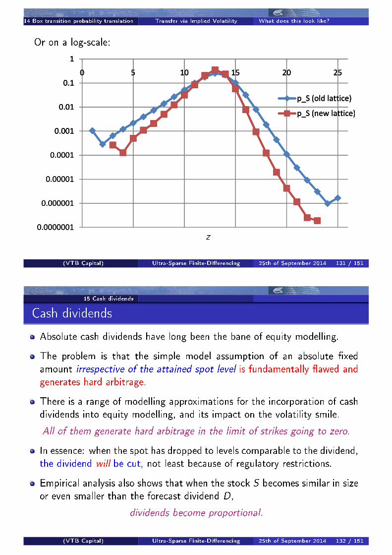
14 Box transition probability translation Transfer via Implied Volatility What does this look like?
Or on a log-scale:
�����
����
���
�
� � �� �� �� ��
�������� ������
��������� ������
���������
��������
�������
������
�����
����
���
�
� � �� �� �� ��
�������� ������
��������� ������
���������
��������
�������
������
�����
����
���
�
� � �� �� �� ��
�������� ������
��������� ������
z
(VTB Capital) Ultra-Sparse Finite-Di�erencing 25th of September 2014 131 / 151
15 Cash dividends
Cash dividends
Absolute cash dividends have long been the bane of equity modelling.
The problem is that the simple model assumption of an absolute �xedamount irrespective of the attained spot level is fundamentally �awed andgenerates hard arbitrage.
There is a range of modelling approximations for the incorporation of cashdividends into equity modelling, and its impact on the volatility smile.
All of them generate hard arbitrage in the limit of strikes going to zero.
In essence: when the spot has dropped to levels comparable to the dividend,the dividend will be cut, not least because of regulatory restrictions.
Empirical analysis also shows that when the stock S becomes similar in sizeor even smaller than the forecast dividend D,
dividends become proportional.
(VTB Capital) Ultra-Sparse Finite-Di�erencing 25th of September 2014 132 / 151
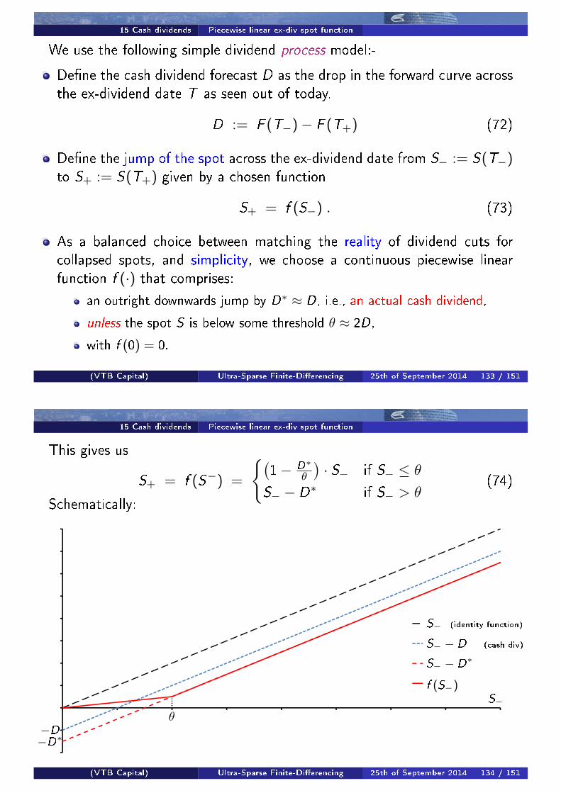
15 Cash dividends Piecewise linear ex-div spot function
We use the following simple dividend process model:-
De�ne the cash dividend forecast D as the drop in the forward curve acrossthe ex-dividend date T as seen out of today.
D := F (T−)− F (T+) (72)
De�ne the jump of the spot across the ex-dividend date from S− := S(T−)to S+ := S(T+) given by a chosen function
S+ = f (S−) . (73)
As a balanced choice between matching the reality of dividend cuts forcollapsed spots, and simplicity, we choose a continuous piecewise linearfunction f (·) that comprises:
an outright downwards jump by D∗ ≈ D, i.e., an actual cash dividend,
unless the spot S is below some threshold θ ≈ 2D,
with f (0) = 0.
(VTB Capital) Ultra-Sparse Finite-Di�erencing 25th of September 2014 133 / 151
15 Cash dividends Piecewise linear ex-div spot function
This gives us
S+ = f (S−) =
{(1− D∗
θ
)· S− if S− ≤ θ
S− − D∗ if S− > θ(74)
Schematically:
S−
−D−D∗
θ
S− (identity function)
S− − D (cash div)
S− − D∗
f (S−)
(VTB Capital) Ultra-Sparse Finite-Di�erencing 25th of September 2014 134 / 151
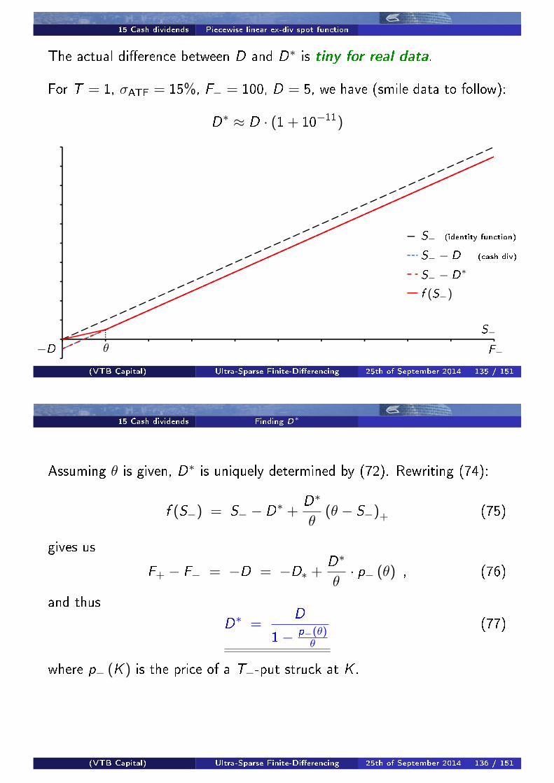
15 Cash dividends Piecewise linear ex-div spot function
The actual di�erence between D and D∗ is tiny for real data.
For T = 1, σATF = 15%, F− = 100, D = 5, we have (smile data to follow):
D∗ ≈ D · (1 + 10−11)
S−
F−−D θ
S− (identity function)
S− − D (cash div)
S− − D∗
f (S−)
(VTB Capital) Ultra-Sparse Finite-Di�erencing 25th of September 2014 135 / 151
15 Cash dividends Finding D∗
Assuming θ is given, D∗ is uniquely determined by (72). Rewriting (74):
f (S−) = S− − D∗ +D∗
θ(θ − S−)+ (75)
gives us
F+ − F− = −D = −D∗ +D∗
θ· p− (θ) , (76)
and thus
D∗ =D
1− p−(θ)θ
(77)
where p− (K ) is the price of a T−-put struck at K .
(VTB Capital) Ultra-Sparse Finite-Di�erencing 25th of September 2014 136 / 151
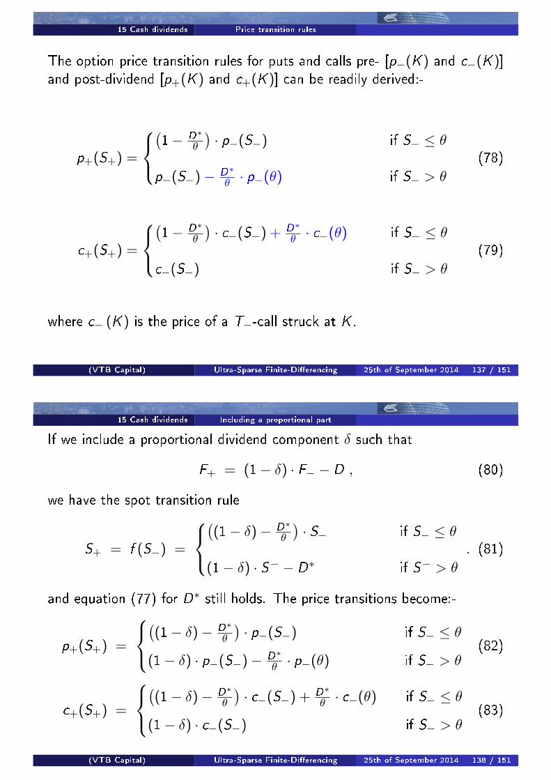
15 Cash dividends Price transition rules
The option price transition rules for puts and calls pre- [p−(K ) and c−(K )]and post-dividend [p+(K ) and c+(K )] can be readily derived:-
p+(S+) =
(1− D∗
θ
)· p−(S−) if S− ≤ θ
p−(S−)− D∗
θ · p−(θ) if S− > θ
(78)
c+(S+) =
(1− D∗
θ
)· c−(S−) + D∗
θ · c−(θ) if S− ≤ θ
c−(S−) if S− > θ
(79)
where c− (K ) is the price of a T−-call struck at K .
(VTB Capital) Ultra-Sparse Finite-Di�erencing 25th of September 2014 137 / 151
15 Cash dividends Including a proportional part
If we include a proportional dividend component δ such that
F+ = (1− δ) · F− − D , (80)
we have the spot transition rule
S+ = f (S−) =
((1− δ)− D∗
θ
)· S− if S− ≤ θ
(1− δ) · S− − D∗ if S− > θ
. (81)
and equation (77) for D∗ still holds. The price transitions become:-
p+(S+) =
((1− δ)− D∗
θ
)· p−(S−) if S− ≤ θ
(1− δ) · p−(S−)− D∗
θ · p−(θ) if S− > θ(82)
c+(S+) =
((1− δ)− D∗
θ
)· c−(S−) + D∗
θ · c−(θ) if S− ≤ θ
(1− δ) · c−(S−) if S− > θ(83)
(VTB Capital) Ultra-Sparse Finite-Di�erencing 25th of September 2014 138 / 151

15 Cash dividends The smile before and after Actual implied volatility smile data
T = 1, β = 0.5, κ = 1, σ = 15%, α = 30%, ρ = −50%, F− = 100, D = 5 (as before):-
10%
15%
20%
25%
30%
35%
40%
45%
50%
0 25 50 75 100 125 150 175 200
sigma(T-)
sigma(T+)
(VTB Capital) Ultra-Sparse Finite-Di�erencing 25th of September 2014 139 / 151
15 Cash dividends The smile before and after Actual implied volatility smile data
Near the money:-
13%
14%
15%
16%
17%
18%
19%
75 100 125
sigma(T-)
sigma(T+)
(VTB Capital) Ultra-Sparse Finite-Di�erencing 25th of September 2014 140 / 151
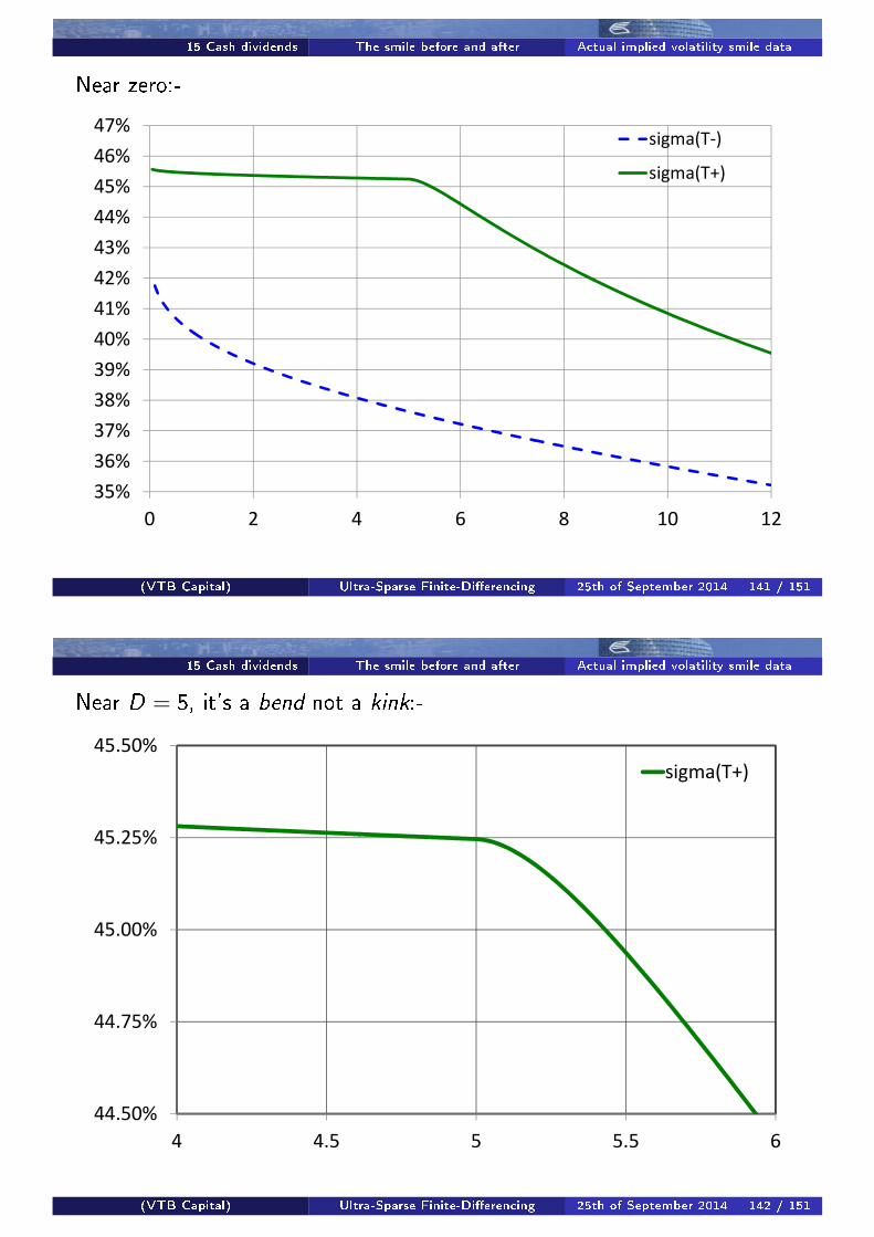
15 Cash dividends The smile before and after Actual implied volatility smile data
Near zero:-
35%
36%
37%
38%
39%
40%
41%
42%
43%
44%
45%
46%
47%
0 2 4 6 8 10 12
sigma(T-)
sigma(T+)
(VTB Capital) Ultra-Sparse Finite-Di�erencing 25th of September 2014 141 / 151
15 Cash dividends The smile before and after Actual implied volatility smile data
Near D = 5, it's a bend not a kink:-
44.50%
44.75%
45.00%
45.25%
45.50%
4 4.5 5 5.5 6
sigma(T+)
(VTB Capital) Ultra-Sparse Finite-Di�erencing 25th of September 2014 142 / 151
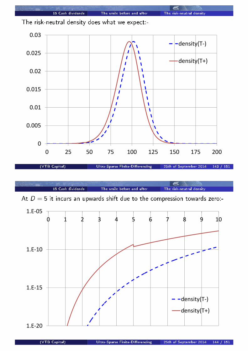
15 Cash dividends The smile before and after The risk-neutral density
The risk-neutral density does what we expect:-
0
0.005
0.01
0.015
0.02
0.025
0.03
0 25 50 75 100 125 150 175 200
density(T-)
density(T+)
(VTB Capital) Ultra-Sparse Finite-Di�erencing 25th of September 2014 143 / 151
15 Cash dividends The smile before and after The risk-neutral density
At D = 5 it incurs an upwards shift due to the compression towards zero:-
1.E-20
1.E-15
1.E-10
1.E-05
0 1 2 3 4 5 6 7 8 9 10
density(T-)
density(T+)
(VTB Capital) Ultra-Sparse Finite-Di�erencing 25th of September 2014 144 / 151
15 Cash dividends Piecewise a�ne dividends in DHI
Within the DHI framework, we can include this piecewise a�ne dividendmodel with great ease using the techniques developed for box transitions!
All we need, is a transition at which we do not change the lattice layout,i.e., a box transition without change in lattice dimensions.
Instead, we populate the probability levels at T+ from option prices struckat the lattice node levels, following the price transitions rules (82) and (83).
This of course requires option prices at T− at strikes at which there are nolattice nodes. For this, we have the implied volatility interpolator at T− asat any other box transition.
All else is already in place! And not a shred of arbitrage!
This is another example where the probability transfer method via trans-formation to an implied volatility smile, and back, is of great use.
(VTB Capital) Ultra-Sparse Finite-Di�erencing 25th of September 2014 145 / 151
16 Conclusion
We presented a framework to e�ectively convert your favourite (smooth) stochas-tic volatility equations into a (quasi-) parametric implied volatility surface.
We used the Hyp-Hyp local-stochastic volatility model.
The purpose is volatility parametrisation and ∆-hedging of vanillas.
The framework is de�ned on a spatial discretisation of an idealised model process.
It is numerically implemented via ultra-sparse �nite di�erencing.
Dynamic Delta largely immunizes against di�erent parameter combinations forthe same smile. It turns out that this is the same as the Local Volatility Delta.
Extensions to normal, as opposed to log-normal, volatilities are possible.
Spatial discretisation gives us a continuous-time-�nite-state Markov chain.
(VTB Capital) Ultra-Sparse Finite-Di�erencing 25th of September 2014 146 / 151
16 Conclusion
A continuous-time perfect martingale from Itô's lemma for pure jump processes.
The importance of being Metzler.
This ensures continuous-time stability and is necessary for positivity preservation.
The seven point stencil for cross-derivatives allows us to remain consistent andstable for all levels of correlation.
Absorbing boundary conditions in all spot-like directions, re�ecting boundary con-ditions for volatility to maximize the use of the grid. No redundancies.
Algebraic operator splitting and anti-di�usive �ux limiting. Keep it physical.
The second order Strang/Padé(0,2) scheme.
Fully implicit and fully Locally-One-Dimensional.
Box transition probability transfer via mapping to implied volatilities, z-marginalbootstrapping from prices, and redistribution in the volatility direction from aconditional probability interpolator.
Also useful for genuinely arbitrage-free cash dividend modelling.
(VTB Capital) Ultra-Sparse Finite-Di�erencing 25th of September 2014 147 / 151
References
[AH11] J. Andreasen and B. Huge.Volatility Interpolation.Risk, March 2011.ssrn.com/abstract=1694972.
[BLOG93] J.P. Boris, A.M. Landsberg, A.S. Oran, and J.H. Gardner.LCPFCT - A Flux-Corrected Transport Algorithm for Solving Generalized Continuity Equations.Technical report, Naval Research Laboratory, April 1993.http://www.dtic.mil/get-tr-doc/pdf?AD=ADA265011.
[CN47] J. Crank and P. Nicolson.A practical method for numerical evaluation of solutions of partial di�erential equations of the heat-conduction type.Proc. Camb. Philos. Soc., 43:50�67, 1947.
[CR76] J. C. Cox and S. A. Ross.The valuation of options for alternative stochastic processes.Journal of Financial Economics, 3:145�166, March 1976.
[CS88] I.J.D. Craig and A.D. Sneyd.An alternating-direction implicit scheme for parabolic equations with mixed derivatives.Comput. Math. Applic., 16:341�350, 1988.www.sciencedirect.com/science/article/pii/0898122188901502.
[Gat04] J. Gatheral.A parsimonious arbitrage-free implied volatility parameterization with application to the valuation ofvolatility derivatives.In ICBI Global Derivatives Conference Madrid, 2004.faculty.baruch.cuny.edu/jgatheral/madrid2004.pdf.
[GJ13] J. Gatheral and A. Jacquier.Arbitrage-free SVI volatility surfaces, March 2013.arxiv.org/pdf/1204.0646.pdf.
(VTB Capital) Ultra-Sparse Finite-Di�erencing 25th of September 2014 148 / 151
References
[Hag13] P. Hagan.Arbitrage-free SABR.WBS 9th Fixed Income Conference, Munich, October 2013.
[Hes93] S. L. Heston.A closed-form solution for options with stochastic volatility with applications to bond and currency options.
The Review of Financial Studies, 6:327�343, 1993.
[HKL02] P. Hagan, D. Kumar, and A. S. Lesniewski.Managing Smile Risk.Wilmott Magazine, pages 84�108, September 2002.
[HV03] W. Hundsdorfer and J.G. Verwer.Numerical Solution of Time-Dependent Advection-Di�usion-Reaction Equations.Springer, 2003.ISBN 3-540-03440-4.
[itHM10] K.J. in 't Hout and C. Mishra.Stability of the Modi�ed Craig�Sneyd scheme for two-dimensional convection-di�usion equations withmixed derivative term.Working paper, University of Antwerp, April 2010.arxiv.org/pdf/1011.6528.pdf.
[itHW09] K.J. in 't Hout and B.D. Welfert.Unconditional stability of second-order ADI schemes applied to multi-dimensional di�usion equations withmixed derivative terms.Appl. Num. Math., 59:677��692, 2009.
[Jäc13a] P. Jäckel.Clamping Down on Arbitrage, December 2013.www.jaeckel.org/ClampingDownOnArbitrage.pdf.
(VTB Capital) Ultra-Sparse Finite-Di�erencing 25th of September 2014 149 / 151
References
[Jäc13b] P. Jäckel.Finite di�erencing schemes as Padé approximants, April 2013.www.jaeckel.org/FiniteDifferencingSchemesAsPad%C3%A9Approximants.pdf.
[Jäc13c] P. Jäckel.Let's be rational.www.jaeckel.org/LetsBeRational.pdf, November 2013.
[JK07] P. Jäckel and C. Kahl.Hyp Hyp Hooray, June 2007.www.jaeckel.org/HypHypHooray.pdf.
[Kuz07] D. Kuzmin.Operator splitting techniques.Technical report, Universität Dortmund, July 2007.www.mathematik.uni-dortmund.de/~kuzmin/cfdintro/lecture11.pdf.
[Kuz10] D. Kuzmin.A Guide to Numerical Methods for Transport Equations.self-published, 2010.www.mathematik.uni-dortmund.de/~kuzmin/Transport.pdf.
[LM78] J.D. Lawson and J.Ll. Morris.The Extrapolation of First Order Methods for Parabolic Partial Di�erential Equations I.SIAM Journal of Numerical Analysis, 15:1212�1224, 1978.www.cs.uwaterloo.ca/research/tr/1977/CS-77-20.pdf.
[LS11] A. Lipton and A. Sepp.Filling the Gaps.Risk, pages 66�71, October 2011.ssrn.com/abstract=2150646.
(VTB Capital) Ultra-Sparse Finite-Di�erencing 25th of September 2014 150 / 151
References
[Min88] H. Minc.Nonnegative Matrices.John Wiley and Sons, 1988.
[MM80] J.D. Macbeth and L.J. Merville.Tests of the Black-Scholes and Cox Call Option Valuation models.Journal of Finance, 35(2):285�301, 1980.efinance.org.cn/cn/fe/19800505Tests%20of%20the%20Black-Scholes%20and%20Cox%20Call%20Option%20Valuation%20Models,%20pp..pdf.
[Rub83] M. Rubinstein.Displaced di�usion option pricing.Journal of Finance, 38:213�217, March 1983.
[Sid98] R. Sidje.Expokit: A Software Package for Computing Matrix Exponentials.ACM Trans. Math. Softw., 24:130�156, 1998.www.maths.uq.edu.au/expokit.
[SS91] E. M. Stein and J. C. Stein.Stock Price Distribution with Stochastic Volatility : An Analytic Approach.Review of Financial Studies, 4:727�752, 1991.
[Str68] G. Strang.On the construction and comparison of di�erence schemes.SIAM J. Numerical Analysis, 5:509�517, 1968.
[SZ99] R. Schöbel and J. Zhu.Stochastic Volatility With an Ornstein Uhlenbeck Process: An Extension.European Finance Review, 3:23�46, 1999.ssrn.com/abstract=100831.
(VTB Capital) Ultra-Sparse Finite-Di�erencing 25th of September 2014 151 / 151