arX

iv:a

stro

-ph/

0211

051v

1 4

Nov

200

2

Ultra-High Energy Gamma Rays in Geomagnetic Field and

Atmosphere

H.P. Vankov1, N. Inoue2 and K. Shinozaki3

1Institute for Nuclear Research and Nuclear Energy, Sofia 1784, Bulgaria

2Department of Physics, Saitama University, Saitama 338-8570, Japan

3Institute for Cosmic Ray Research, University of Tokyo, Chiba 277-8582, Japan

(May 28, 2018)

Abstract

The nature and origin of ultra-high energy (UHE: referring to > 1019 eV)

cosmic rays are great mysteries in modern astrophysics. The current theories

for their explanation include the so-called ”top-down” decay scenarios whose

main signature is a large ratio of UHE gamma rays to protons. Important step

in determining the primary composition at ultra-high energies is the study of

air shower development. UHE gamma ray induced showers are affected by the

Landau-Pomeranchuk-Migdal (LPM) effect and the geomagnetic cascading

process. In this work extensive simulations have been carried out to study

the characteristics of air showers from UHE gamma rays. At energies above

several times 1019 eV the shower is affected by geomagnetic cascading rather

than by the LPM effect. The properties of the longitudinal development such

as average depth of the shower maximum or its fluctuations depend strongly

on both primary energy and incident direction. This feature may provide a

possible evidence of the UHE gamma ray presence by fluorescence detectors.

1

I. INTRODUCTION

The ultra-high energy (UHE; > 1019 eV) cosmic ray research has been initiated about

40 years ago. Several experiments have been carried out and at present AGASA [2], HiRes

[3] and Yakutsuk [4] experiments are in operation to observe air showers initiated by UHE

cosmic rays (see for a review [1]). Today the number of recorded events is already big enough

to convince even strong sceptics that the cosmic ray energy spectrum extends well beyond

the theoretically expected Greisen-Zatzepin-Kuz’min (GZK) cutoff around 5 × 1019 eV [5].

The origin and nature of these particles are still unsolved questions. The problem is that it is

very difficult to extend our understanding of particle acceleration to such extraordinary high

energies and the propagation of these particles in the cosmic microwave background (CMB)

radiation restricts the distance to their potential sources within several tens of megaparsecs

(1 Mpc = 3.1× 1024 cm).

Various models of UHE cosmic ray origin have been proposed. They are currently a

subject of very intensive discussion (see for a review [6]). Models can be categorized into

two basic groups of “scenarios”: “bottom-up” and “top-down”.

Conventional “bottom-up” scenarios look for astrophysical sources called “Zevatrons”

(1 Z eV = 1021 eV) that can accelerate particles to energies in excess of 1020 eV. The

composition of UHE cosmic rays is expected to be hadronic. Possible candidates include

clusters of galaxies, active galactic nuclei (AGN) radio lobes, AGN central regions, young

neutron stars, magnetars, gamma ray bursts, etc.

In the “top-down” scenarios UHE cosmic rays instead of being accelerated are generated

from decay of some exotic very heavy (1022 – 1025 eV) X-particles that are supposed to have

been formed in the early universe. The sources of X-particles may be topological defects

(cosmic strings, cosmic necklaces, magnetic monopoles, domain walls) [7] or long-lived super-

heavy relic particles [8].

The cascade process initiated by a super-high energy neutrino (∼ 1022 eV) in the relic

neutrino background (the so-called Z-burst model) [9] is another possible scenario which is

2

a hybrid of astrophysical Zevatrons with new particles [10].

In general, “top-down” and “hybrid” scenarios predict a rather high flux of UHE neu-

trinos exceeding the observed cosmic ray flux. Gamma rays account for a part or most of

the highest energy cosmic rays above 1020 eV, whereas nucleons would dominate at lower

energies. Thus the primary composition, especially the gamma ray content (reffered to as

gamma/proton ratio), is a powerful discriminator between the models of the UHE cosmic

ray origin. It should be mentioned that even within conventional ”bottom-up” models one

can expect a significant gamma/proton ratio due to the decay of neutral pions produced in

cosmic ray interactions with the 2.7 K CMB photons. Under certain circumstances (extra-

galactic magnetic field strength, distance to the sources, maximal proton energy, slope of the

proton energy spectrum, etc.), the subsequent electromagnetic cascade in the intergalactic

space can lead to a UHE gamma ray flux comparable to the observed cosmic ray flux [11,12].

Air showers initiated by UHE gamma rays have characteristic features in comparison

with “ordinary” hadronic showers. Two effects must be taken into account for a study of air

shower development in case of gamma ray primaries —– the Landau-Pomeranchuk-Migdal

(LPM) effect and cascading in the geomagnetic field.

The influence of the LPM effect [13,14] on shower development has been studied by

many authors during the last thirty years. The effect reduces the Bethe-Heitler (BH) cross

sections for bremsstrahlung and pair production at energies >∼ 1019 eV in the atmosphere

leading to a significant elongation of the electromagnetic shower and large fluctuations in

the shower development. Generally, this effect is well understood although there is no

commonly accepted standard code taking into account the LPM effect in electromagnetic

shower modeling. It should be pointed out that other possible mechanisms of suppression

of bremsstrahlung and pair creation processes at extremely high energies have to be more

carefully studied [15].

Once the electron-positron pair is produced in UHE gamma ray interaction with the

geomagnetic field away from the Earth’s surface, it initiates an electromagnetic ”cascade”

due to synchrotron radiation before entering the atmosphere. As a result, the energy of

3

the primary gamma ray is shared by a bunch of lower energy secondary particles which

are mainly photons and a few electron-positron pairs. The influence of the LPM effect on

subsequent showers in the atmosphere is significantly weakened.

The history of electromagnetic cascade calculations in the geomagnetic field is also long

enough since it started with the work of McBreen and Lambert [16]. The main results of

previous works [12,17–20] are in a good agreement . Recent calculations refined the previous

ones revealing some practically important features in the cascading process. For example,

in [21] it is shown that the study of two major components of the giant air showers, the

size spectra and muon content, can reveal the nature of the UHE cosmic rays if the spe-

cific dependence on the shower arrival direction is observed. Some observables that can be

extracted from the Pierre Auger Observatory detectors (longitudinal profiles, lateral distri-

bution and front curvature) are discussed in [22]. In [23] the technique of adjoint cascade

equations was applied to study UHE gamma ray shower characteristics in the geomagnetic

field and in the atmosphere emphasizing the muon component of air shower.

The aim of the present paper is to study in details the UHE gamma ray shower char-

acteristics that are measurable by air fluorescence detectors. It is also important to know

the difference in longitudinal shower development between gamma ray and hadronic show-

ers which can be used for an effective separation between these primary species. In the

following, we will discuss the dependence of UHE gamma ray shower characteristics on the

incident direction and the possibility of detecting such showers in the future experiments.

II. ELECTROMAGNETIC INTERACTIONS IN MAGNETIC FIELD

About sixty years ago soon after Auger’s discovery of the extensive air showers, Pomer-

anchuk [24] estimated the maximal energy of primary cosmic ray electrons and gamma rays

that is allowed to enter the atmosphere after interactions with geomagnetic field. According

to his calculations, the maximal electron energy Ec due to radiation in the geomagnetic field

is a few times 1017 eV (∼ 4 × 1017 eV for vertically incident electrons on the geomagnetic

4

equatorial plane). Whatever energy greater than Ec electrons have, they lose their energies

rapidly down to below Ec. The analogous gamma ray energy due to pair creation in the

geomagnetic field is ∼ 6× 1019 eV.

Similar to cascading in matter, the main elementary processes leading to particle multi-

plication in magnetic field are magnetic bremsstrahlung (synchrotron radiation) and mag-

netic pair production. It is well known that essentially non-zero probabilities for magnetic

bremsstrahlung and pair production require both strong field and high energies [25]. The

relevant parameter determining the criteria for this is:

χ =E

mc2H⊥

Hcr(1)

where E is the particle energy, H⊥ is the magnetic field strength (the component perpen-

dicular to the particle trajectory), m is the electron mass and Hcr = 4.41× 1013 G.

The total probabilities (cross sections) for radiation and pair production for a given

value of the magnetic field strength depend only on χ and are shown in Fig. 1. Magnetic

pair production has significant probability for χ ≥ 0.1. For effective shower development,

however, one needs even higher values of χ ≥ 1 because the radiated photon spectrum

becomes harder with increasing χ. The maximal photon energy estimated by Pomeranchuk

(∼ 6× 1019 eV) comes from the condition χ ∼ 1.

We use the expressions of Bayer et al. [26] for the differential probabilities (per unit

length) for magnetic bremsstrahlung and magnetic pair production:

π (ε, ω) dω =αm2

π√3

dω

ε2

(

ε− ω

ε+

ε

ε− ω

)

K 2

3

(

2u

3χ

)

−∞∫

2u

3χ

K 1

3

(y) dy

(2)

for bremsstralung, and

γ (ω, ε)dε =αm2

π√3

dε

ω2

(

ω − ε

ε+

ε

ω − ε

)

K 2

3

(

2u1

3χ

)

+

∞∫

2u1

3χ

K 1

3

(y) dy

(3)

for pair creation, where ε and ω are the electron and photon energies and u = ω/(ε − ω),

u1 = ω2/ε(ω − ε). Here h̄ = c = 1. Kν (z) =∞∫

0e−zch(t)ch (νt) dt is the modified Bessel

function known as MacDonald’s function.

5

While for χ ≫ 1 (strong field) the electromagnetic cascade develops similar to the cas-

cade in matter [27], in case of χ ≤ 1 the photon interaction length increases sharply with

decreasing photon energy. Electrons continue to radiate and the shower becomes a bunch

of secondary photons carrying more than 94− 95% of the primary energy.

III. SIMULATION

In our simulation studies of air showers initiated by gamma rays and hadrons (proton

or iron), we use the AIRES code (version 2.2.1) [28] incorporated with QGSJET hadronic

interaction model [29]. AIRES includes the LPM effect in simulation of electromagnetic

showers. For simulations of electromagnetic cascades in the geomagnetic field we use our

original code.

To simulate showers initiated by UHE gamma rays, we first model cascading in the geo-

magnetic field starting with a single UHE gamma ray far away from the Earth’s surface down

to the top of the atmosphere. Then secondary particles that reach the top of atmosphere

are set as an input for the AIRES code. Finally, the air shower initiated by the UHE gamma

ray is constructed as a superposition of lower energy gamma ray sub-showers. In practice,

we use a library of pre-simulated showers in the atmosphere which has been calculated by

the AIRES code.

A. Electromagnetic cascading in geomagnetic field

We simulate the electromagnetic cascade in the geomagnetic field by injecting a UHE

gamma ray at a distance of 3Re away from the Earth’s surface where Re is the Earth’s

radius of 6.38 × 108 cm. The primary gamma ray and secondary particles are propagated

by taking account of pair production and synchrotron radiation on each step (a step-size

of 1km). Only particles above a threshold energy of 1016 eV are followed in the simulation

until they reach the top of the atmosphere. This threshold energy is low enough to neglect

the contribution of sub-threshold particles in the cascade.

6

In order to examine the properties of electromagnetic cascades as a function of the

incident direction, we divide uniformly the sky by bins of 5◦ for both azimuth and zenith

angles to 1085 points and simulate 50 events for each point. In our simulation we use the

International Geomagnetic Reference Field (IGRF) and World Magnetic Model (WMM)

which provide a good approximation for the geomagnetic field up to 600 km above sea level

[30]. Above this altitude the geomagnetic field is extrapolated from this model.

In the present work we examine the properties of UHE gamma ray showers for the

location of Utah, USA (Long. = 113.0◦ W, Lat. = 39.5◦N and 1500 m above sea level) near

the site of the HiRes experiment. In this location, IGRF gives the field of 0.53 G pointing

25◦ downword from 14◦ east of the geographical (true) north.

B. Atmospheric shower simulation

The simulations of atmospheric showers are carried out independently from the geo-

magnetic cascading process. Using AIRES code, we first prepare a library of sub-showers

initiated by gamma rays with zenith angles of 39.7◦, 54◦ and 61.6◦ and energy fixed be-

tween 1016 and 1021 eV at logarithmically equally spaced values (10 energies per decade).

The number of all charged particles are recorded at 5 g cm−2 intervals in vertical depth.

The library contains 500 showers at each energy. It should be noted that this number is

significantly greater than the maximal number (∼ 100) of secondary gamma rays from the

geomagnetic cascade in each energy bin.

The construction of UHE gamma ray initiated shower is carried out by a method similar

to the so-called ”boot-strap” method as following: i-th secondary particle with energy E(GM)i

at the top of atmosphere is followed by a sub-shower with the nearest energy E(atm)i selected

randomly from the library. The secondary electron is replaced by a gamma ray with the

same energy. By summing up the sub-showers (i = 1, . . . , N (GM)γ ) with a weight wi =

E(GM)i /E

(atm)i , the atmospheric shower initiated by a single gamma ray with energy E

(γ)0 is

represented as a superposition of sub-showers with total energyNγ∑

wiE(atm)i = E

(γ)0 .

7

In the present work we also aimulate amples of 500 hadron (proton and iron) initiated

showers for the same zenith angles and energy range to compare the results.

IV. RESULT

A. Properties of geomagnetic cascading

The cascade development is determined by the features of the cross sections of the pro-

cesses and the field strength. The maximal values of the parameter χ which governs cascad-

ing do not much exceed 1, e.g. χ = 1.33 for 1020 eV and H⊥ = 0.3 G, and χ = 13.3 for 1021

eV and same H⊥, i.e. one can expect only a few gamma ray interactions (pair creations)

in the shower. But such H⊥ values are characteristic for the surface of the Earth. The

field strength rapidly decreases with the geocentric distance, ∼ 1/Re, which means that the

cascade starts not far from the surface of the Earth. The first interaction of the gamma rays

with the energies of interest occurs in relatively narrow range of distances not further than

3Re . For example, the mean altitude of the first interaction of vertical gamma rays with

primary energy E(γ)0 = 1021 eV is about 5300 km.

The typical shower profiles averaged over 1000 showers for E(γ)0 = 1020 eV and different

threshold energies for secondary photons and electrons are shown in Fig. 2 (bottom panel).

The zenith angle is 40◦ and the azimuth corresponds to north (strong field). For comparison

in this figure is also shown the shower profile for the secondary photons with energy above

1016 eV in a shower coming from south (weak field). This picture differs too much from the

cascade development in the matter. As the primary energy distributes between the electron

and photon components (see the top panel of Fig. 2), the mean photon energy decreases

and when χ < 1 the mean free path for pair production sharply increases (see Fig. 1). The

energy of the electron component starts to return quickly to the photon component and the

shower converts to a beam of photons carrying the bulk of the primary energy. For the case

shown in Fig. 2 (strong field) the mean number of gamma ray interactions per shower in

8

the geomagnetic field is approximately 1 (1.11 for the sample of 1000 showers) which means

that there is almost no pair creation after the initial interaction. For E(γ)0 = 5 × 1020 eV

and same conditions this number increases to 4.16. This is the reason for the much smaller

number of electrons than photons in the shower. In our example, for the strong field, the

mean number of electrons reaching the top of the atmosphere, is 2.22 (=2 × 1.11) for 1016

eV threshold energy. These electrons carry ∼ 2% of the primary energy. In the case of weak

field (line with symbols in Fig. 2), the probability of the primary gamma ray to interact in

the geomagnetic field is only ∼ 6− 7% and this happens on an average of 200 km from the

sea level.

In Utah, the southern sky region is close to the direction of the geomagnetic field and

hence the effect of geomagnetic cascading is relatively small. Gamma rays arriving from the

northern sky region travel through stronger field whose strength increases with the zenith

angle. Generally, primary gamma rays are most affected by the geomagnetic field when they

come from the northern sky or near the horizon.

Fig. 3 shows maps for the gamma ray conversion (interaction) probability (grey scale)

with the geomagnetic field for all incident directions in horizontal coordinates. The different

panels correspond to primary energies E(γ)0 = 1019.5, 1020, 1020.5 and 1021 eV. The radial

coordinate is the zenith angle θ. The inner circles correspond to θ = 30◦ and 60◦, and the

outer one is of the horizon. Azimuths are as labeled ‘N’ denotes the true north). Dashed

curves indicate the opening angles of 30◦, 60◦ and 90◦ to the local magnetic field.

The region with smaller probability is around the direction which is parallel to the

local geomagnetic field. From this region, primary gamma rays are most likely to enter

the atmosphere without interaction. Thus, this region can be referred to as “window” for

the primary gamma rays. Through this window they can reach the top of the atmosphere

surviving interaction and be observed as ‘LPM showers’. The size of this window shrinks

rapidly with increasing primary energy and almost all gamma rays with E(γ)0

>∼ 1020 eV

initiate a geomagnetic cascade above the atmosphere.

Fig. 4 shows maps of the average multiplicity of the secondary particles (number of

9

electrons plus photons above 1016 eV; grey scale) at the top of atmosphere on the same

coordinates as in Fig. 3. The average energy of secondary particles (E(γ)0 /multiplicity) is

plotted in Fig. 5.

The patterns of these maps match well the field strength, i.e. the direction of the

geomagnetic field at the ground level, which reflects the fact that the first interaction occurs

not far from the Earth’s surface.

For low primary energy and/or weak field strength, i.e. small E(γ)0 H⊥, the primary

gamma ray does not or only once produces electron-pair before reaching the top of the atmo-

sphere. The produced electrons continuously radiate photons by magnetic bremsstrahlung

and the multiplicity increases with the primary energy. Nevertheless, radiated photons can

hardly interact again with the geomagnetic field unless χ >∼ 1.

For the direction with very strong field (or very high primary energy), i.e. large E(γ)0 H⊥,

e.g. for the northern sky region or near-horizontally incident gamma rays, the multiplicity is

almost proportional to the primary energy which leads to a nearly constant average particle

energy at the top of the atmosphere (see Fig. 5). This energy is about a few times of 1017

eV. In the sky regions where the conversion probability is 100% the maximal average energy

of the secondary particles, which are mainly photons, do not exceed several times 1019 eV.

This is consistent with the estimation by Pomeranchuk [24] described previously and thus

the LPM effect is ineffective in the atmosphere except for the window regions.

The multiplicity distribution of secondary particles at the top of the atmosphere for

different incident zenith angles (39.7◦, 54◦ and 61.6◦) and azimuths corresponding to north

and south, are plotted in Fig. 6. Each histogram includes 1000 simulated showers.

The columns in the first bin of each panel correspond to the primary gamma rays that

do not interact in the geomagnetic field. In regions with 100% conversion probability the

fluctuations are small for large E(γ)0 H⊥ due to the better cascade development by the more

gamma ray interactions above the astmosphere.

Fig. 7 shows the average energy distribution (spectrum) of secondary particles at the

top of the atmosphere. The data belong to the same set of simulated showers as in Fig. 6.

10

Here the ‘surviving’ primary gamma rays manifest themselves by the columns in the last

bins of some histograms.

The maximum of the spectrum shifts towards the higher energies when E(γ)0 increases.

However, except for the cases where the probability of survival primaries is large, i.e. the

conversion probability is not close to 100%, this shift slows down for E(γ)0 > 1020 eV and

the shape of the spectrum remains almost same for the highest energies. As mentioned

previously, the multiplicity of secondaries is almost proportional to E(γ)0 . The spectra display

sharp cutoff at a few times 1019 eV and subsequent sub-showers in the atmosphere are not

affected by the LPM effect. We discuss this in the next subsection.

We estimate the lateral spread of particles at the top of the atmosphere. All particles are

contained within a radius of about 10 cm. This value is much greater than 0.1 mm given in

[16,19] but is still too small to be taken into account. Thus, successive shower developments

in the atmosphere can be correctly expressed as a superposition of atmospheric sub-showers

initiated by secondary particles with such energy spectra.

B. Shower development in the atmosphere

Fig. 8 shows examples of individual shower developments initiated by primary gamma

rays with Eγ0 = 1019, 1020 and 1021 eV. Left and right panels correspond to azimuths from

north and south, respectively. Zenith angles are 39.7◦, 54◦ and 61.6◦. Dashed curves repre-

sent the average shower profiles for proton primaries.

This figure illusrates very well a remarkable feature of the shower development at these

energies — significantly small fluctuations in the case that the primary gamma ray interacts

with the geomagnetic field. The largest fluctuations in the shower development can be found

for Eγ0 = 1020 eV, θ = 39.7◦ and incident direction from south. In this case the primary

gamma ray conversion probability in the geomagnetic field is only several percent and the

LPM effect affects strongly the shower development in the atmosphere. Increasing primary

energy leads to significant decrease of fluctuations and this trend is stronger for the sky

11

regions close to the horizon (large H⊥). These two effects are more pronounced for northern

sky regions.

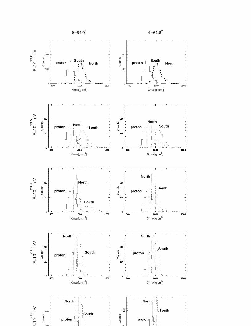
Fig. 9 shows distributions of the average depth of the shower maximum in the atmosphere

〈Xmax〉 for showers with E(γ)0 = 1019, 1019.5, 1020, 1020.5 and 1021 eV. We present the cases of

zenith angles of 54◦ and 61.6◦ in left and right panels, respectively. In each panel, the solid

line indicates the distribution of proton showers. Dotted and dashed lines represent those

for gamma ray showers from azimuths of north and south, respectively.

The shape of 〈Xmax〉 distributions of gamma ray showers noticeably varies with primary

energy and incident direction. As the primary energy increases, the distributions become

narrower and the mean values are almost constant for energies > 1020 eV (see also Fig. 11).

Some distributions having two maxima or long tail to the deeper Xmax result from a mixture

of converted and not-converted gamma rays above the atmosphere.

In Fig. 10, maps of Xmax are shown on the same coordinates as in Figs. 3 – 5.

The data for this figure are obtained by the following approximation. The simulation

of the shower development is based on the method described in the previous section. For a

given zenith angle we use data from the library of pre-simulated showers with similar zenith

angle. Since the magnitude of the LPM effect depends on the atmospheric density profile

along the particle trajectory, there is a small dependence on the incident zenith angle. In

the vertical region for 1020 eV, this effect possibly matters and 〈Xmax〉 can be higher than

shown due to the lack of air shower library for this direction. For higher primary energy or

other sky region, however, primary gamma rays are converted and thus it is not necessary

to take into account the LPM effect for the estimation of 〈Xmax〉.

In each map, i.e. for each E(γ)0 , 〈Xmax〉 reflects the dependence of geomagnetic cascading

on the incident direction. Typically, gamma ray showers with larger 〈Xmax〉 are predomi-

nantly coming from southern sky region. Only for 1020 eV there is a small window where

gamma ray showers are affected by the LPM effect. This region may serve as a probe for

UHE gamma ray presence.

Fig. 11 shows the relation between 〈Xmax〉 and E(γ)0 for gamma ray showers. For com-

12

parison, corresponding relations for proton and iron primaries are also drawn in the figure.

Incident azimuths of gamma rays are from north and south. Dashed lines and thick solid

lines are for zenith angles of 54◦ and 61.6◦, respectively. The dotted curve indicates the case

of no geomagnetic field.

For proton and iron showers 〈Xmax〉 increases with E(γ)0 and the slope of the relation,

i.e. the elongation rates are almost constant and are 54 and 56 g cm−2/decade, respectively.

The elongation rate for gamma ray showers is greater than those of hadronic ones and is

also constant according to the electromagnetic cascade theory up to energies ∼ 2× 1019 eV.

Above this energy the LPM effect steepens the relation of 〈Xmax〉 versus E(γ)0 as shown by

the dotted line in the figure.

The geomagnetic cascading starts to “work” approximately at the same energy, about

several times 1019 eV. At this energy which depends on the incident direction, 〈Xmax〉 reaches

its maximum. Above this energy the geomagnetic cascade develops well enough to suppress

the LPM effect in the atmosphere. This leads to a rapid decrease of 〈Xmax〉.

The slow increase of 〈Xmax〉 after its minimum results from the slow increase of the

fraction of secondary photons above the threshold for the LPM effect (see Fig. 7). The

multiplicity also increases proportionally to E(γ)0 which leads to almost constant average

photon energy in the bunch above 1020 eV. It must be noted that a superposition of BH

sub-showers has smaller 〈Xmax〉 than a single BH shower with an energy equal to the sum

of the sub-shower energies.

In Fig. 12, the fluctuations of Xmax (the standard deviation of Xmax distribution) are

shown as a function of primary energy . The line key is the same as in Fig. 11 but the case

of no geomagnetic field is not shown.

Similar to 〈Xmax〉, the fluctuations for gamma ray showers vary typically depending on

primary energy and incident direction, while those for proton and iron showers are almost

constant, ∼ 67 g cm−2 and ∼ 26 g cm−2, respectively.

For gamma ray showers, the picture between 1919 and 1020 eV is similar to that in Fig.

11. Large fluctuations are due to the LPM effect. For energies at which the geomagnetic

13

cascading is effective, the fluctuations decrease rapidly with the energy. At the highest

energies, the fluctuations tend to be as small as those for iron showers. This behavior

attributes to a competition between the LPM effect and geomagnetic cascading as in Fig.

11.

V. DISCUSSION AND CONCLUSIONS

Our study shows that the longitudinal development of gamma ray showers is not simply

scaled with primary energy. Shower development in the energy region above ∼ 1019.5 eV

shows very specific dependence both on the primary energy and incident direction. 〈Xmax〉

of gamma ray showers is larger than that expected for proton showers. Furthermore, the

elongation rate of gamma ray showers shows considerable variation with energy depending on

their incident directions. The future observation of these longitudinal shower characteristics

with better statistical accuracy would be the possible key for studying the UHE gamma ray

flux. Also, additional information may be obtained from the properties of Xmax fluctuations.

In order to acquire a definite conclusions of the primary composition of UHE cosmic rays,

more elaborate considerations may be required due to a limited statistics and difficulty in

separating between gamma ray and hadronic showers. For example as is shown above, the

fluctuations of Xmax for gamma ray showers become even less than those for proton showers

and are close to iron showers above 1020 eV. We expect that the development of a number

of UHE showers would be measured with a better accuracy in the near future which will be

the first decisive step in looking for UHE gamma rays.

If the observed showers develop slowly from the sky region nearby the window (see Figs.

2 – 4 and 9) showing typical characteristics of LPM showers, this could be a noticeable and

physically important evidence of the UHE gamma ray presence.

As was earlier mentioned in [21], magnetic bremsstrahlung process may be important for

the shower development at high altitudes where the atmospheric density is very low. Ac-

cording to the estimations in [31], made by numerical integration of the system of cascade

14

equations, the interaction of shower particles with the geomagnetic field inside the atmo-

sphere becomes important for cascades created by primary gamma rays with energies higher

than ∼ 3× 1020 eV. For example, injecting the gamma rays with energy 1020 eV vertically

into the atmosphere, the number of particles in showers at sea level calculated only with

LPM effect is ∼ 13% less than that in showers when interactions with the geomagnetic

effect (for H⊥ = 0.35 G) taken into account. This difference increases with the primary

energy up to ∼ 2.5 times for 1021 eV. Using our own simple hybrid code for one-dimensional

atmospheric shower simulation we obtain similar results showing also a noticeable shift of

the shower maximum. This work is now in progress.

Planned projects (Auger [32], EUSO [33], etc.) to study UHE cosmic rays promise

to observe individual shower development with better accuracy. It is important to find the

effective and reasonable physical parameters from simulation studies in order to discriminate

gamma ray showers from hadronic ones on event by event basis. It can be also strong

probe by including the fluctuation study in addition to average shower development in the

discussions about the composition of UHE cosmic rays.

ACKNOWLEDGMENTS

We thank T. Stanev for valuable help and discussions. H.P.Vankov is thankful to Japan

Society for the Promotion of Science(JSPS) for support of his visit to Japan where this work

was conceived, and to the National Graduate Institute for Policy Study (GRIPS) for its

hospitality.

15

REFERENCES

[1] M. Nagano and A.A. Watson , Rev. Mod. Phys. 72, 689 (2000).

[2] H. Ohoka et al., Nucl. Instrum. Meth. A 385, 268 (1997).

[3] C.C.H. Jui et al., inProceedings of the 27th International Cosmic Ray Conference,

Hamburg, Germany, Vol. 1, 354 (2001).

[4] B.N. Afanasiev et al., in Proceedings of the Tokyo Workshop on Techniques for the Study

of the Extremely High Energy Cosmic Rays, Tanashi, Tokyo, 1993, edited by M. Nagano

(Institute of Cosmic Ray Research, University of Tokyo), p.32.

[5] K. Greisen, Phys. Rev. Lett. 16, 748 (1966) ; G.T. Zatsepin and V.A. Kuz’min, Pis’ma

Zh. Eksp. Teor. Fiz. 4, 114 (1996) [JETP Lett. 4, 78 (1966)].

[6] P. Bhattachrjee and G. Sigl, Phys. Rept. 327, 109 (2000) and references therein.

[7] P. Bhattacharjee, C.T. Hill, and D.N. Schramm, Phys. Rev. Lett. 69, 567 (1992) .

[8] V. Berezinsky, P. Blasi and A. Vilenkin, Phys. Rev. D 58, 103515 (1998) .

[9] T.J. Weiler, Phys. Rev. Lett. 49, 234 (1982) .

[10] A. Olinto, http://xxx.lanl.gov/astro-ph/0201257.

[11] F. Halzen, R. Protheroe, T. Stanev and H. Vankov, Phys. Rev. D 41, 343 (1990) ; J.

Wdowczyk and A.W. Wolfendale, Astrophys. J. 349, 35 (1990).

[12] F.A. Aharonian, B.L. Kanewsky and V.V. Vardanian, Astrophys. Space. Sci. 167, 111

(1990) .

[13] L.D. Landau and I.J. Pomeranchuk, Dokl. Akad. Nauk. SSSR 92, 535 (1953) (in Rus-

sian).

[14] A.B. Migdal, Phys. Rev. 103, 1811 (1956) .

[15] S. Klein, Rev. Mod. Phys. 71, 1501 (1997) .

16

[16] B. McBreen and C.J. Lambert, Phys. Rev. D 24, 2536 (1981).

[17] H.P. Vankov and P. Stavrev, Phys. Lett. B 266, 178 (1991) .

[18] S. Karakula and W. Bednarek, in Proc. of 24th International Cosmic Ray Conference,

Rome, Italy, Vol.1, 266 (1995).

[19] K. Kasahara, in Proceedings of International Symposium on EHECR: Astrophysics and

Future Observations, Tanashi, Tokyo, Japan, 1966, edited by M. Nagano (Institute for

Cosmic Ray Research, University of Tokyo 1997), p. 221.

[20] W. Bednarek, http://xxx.lanl.gov/astro-ph/9911266; astro-ph/011061.

[21] T. Stanev and H.P. Vankov, Phys. Rev. D 55, 1365 (1997) .

[22] X. Bertou, P. Billoir and S. Dagoret-Campagne, Astropart. Phys. 14, 121 (2000) .

[23] A.V. Plyasheshnikov and F.A. Aharonian, J. Phys. G: Nucl. Part. Phys. 238, 267 (2002)

.

[24] I. Pomeranchuk, Pis’ma Zh. Eksp. Teor. Fiz. 9, 915 (1939) (in Russian).

[25] T. Erber, Rev. Mod. Phys. 38, 626 (1966) .

[26] V.H. Bayer, B.M. Katkov and V.S. Fadin, Radiation of Relativistic Electrons (Atomiz-

dat, Moscow, 1973) (in Russian).

[27] V. Anguelov and H. Vankov, J. Phys. G: Nucl. Part. Phys. 25, 1755 (1999) .

[28] S.J. Sciutto, http://xxx.lanl.gov/astro-ph/9911331).

[29] N.N. Kalmykov and S.S. Ostapchenko, Phys. At. Nucl. 56(3), 346 (1993) .

[30] Distributed by National Geophysical Center, USA, http://www.ngdc.noaa.gov.

[31] B.L. Kanevsky and A.I. Goncharov, Voprosy atomnoy nauki i techniki, Ser.:Tehnika.

fiz.eksperimenta, 1989, vyp.4(4), 34; A.I. Goncharov, Thesis, Tomsk Polytechnical In-

17

stitute, 1991 (in Russian).

[32] AUGER Collaboration, Website: www.auger.org.

[33] EUSO Collaboration, Website: www.ifcai.pa.cnr.it/˜EUSO/.

18

FIGURES

0.1 1 10 100 100010

-11

10-10

10-9

10-8

10-7

10-6

10-5

brem

pair

Inte

ract

ion

prob

abili

ty [

cm

G

]

-1

-1

χ

FIG. 1. The total probabilities (cross sections) for magnetic bremsstrahlung and pair produc-

tion as a function of parameter χ.

19

0.01

0.1

1

10

100

0.0

0.1

0.9

1.0

Ene

rgy

flux

/ Eγ

3

21

3

2

1E

γ = 1020 eV

0.5 01

Num

ber

of p

artic

les

distance to the Earth, Re

FIG. 2. Shower profile (bottom panel) in the geomagnetif field for primary gamma ray with

energy 1020 eV and different threshold energies: 1—1016 eV, 2—1019 eV and 3—5× 1019 eV. The

zenith angle is 40◦ and the azimuths corresponds to the north. Solid and dotted curves indicates

for photons and electrons, respectively. Curves with symbols show the number of photons with

energies > 1016 eV in showers with the same primary energy and azimuth from the south. The

energy flux carried by photons (solid curve) and electrons (dotted curve) is shown on the top panel

for azimuth from the north. Re is the Earth’s rudius(= 6.38 × 108cm).

20

Conversion Probability0 50 100%

Conversion Probability0 50 100%

Conversion Probability0 50 100%

Conversion Probability0 50 100%

Conversion Probability0 50 100%

Conversion Probability0 50 100%

Conversion Probability0 50 100%

Conversion Probability0 50 100%

Conversion Probability0 50 100%

Conversion Probability0 50 100%

Conversion Probability0 50 100%

Conversion Probability0 50 100%

N

W

S

E

Conversion Probability0 50 100%

Conversion Probability0 50 100%

Conversion Probability0 50 100%

Conversion Probability0 50 100%

Conversion Probability0 50 100%

Conversion Probability0 50 100%

Conversion Probability0 50 100%

Conversion Probability0 50 100%

Conversion Probability0 50 100%

Conversion Probability0 50 100%

Conversion Probability0 50 100%

Conversion Probability0 50 100%

N

W

S

E

Conversion Probability0 50 100%

Conversion Probability0 50 100%

Conversion Probability0 50 100%

Conversion Probability0 50 100%

Conversion Probability0 50 100%

Conversion Probability0 50 100%

Conversion Probability0 50 100%

Conversion Probability0 50 100%

Conversion Probability0 50 100%

Conversion Probability0 50 100%

Conversion Probability0 50 100%

Conversion Probability0 50 100%

N

W

S

E

Conversion Probability0 50 100%

Conversion Probability0 50 100%

Conversion Probability0 50 100%

Conversion Probability0 50 100%

Conversion Probability0 50 100%

Conversion Probability0 50 100%

Conversion Probability0 50 100%

Conversion Probability0 50 100%

Conversion Probability0 50 100%

Conversion Probability0 50 100%

Conversion Probability0 50 100%

Conversion Probability0 50 100%

N

W

S

E

E=10 [eV]19.5 21.020.520.0E=10 [eV] E=10 [eV] E=10 [eV]

FIG. 3. Maps of gamma ray conversion probability in the geomagnetic field for primary energies

1019.5, 1020, 1020.5 and 1021 eV. Inner circles correspond to zenith angles 30◦, 60◦ and horizon.

1 10 100 1000 10000

Multiplicity1 10 100 1000 10000

Multiplicity1 10 100 1000 10000

Multiplicity1 10 100 1000 10000

Multiplicity1 10 100 1000 10000

Multiplicity1 10 100 1000 10000

Multiplicity1 10 100 1000 10000

Multiplicity1 10 100 1000 10000

Multiplicity1 10 100 1000 10000

Multiplicity

N

W

S

E

1 10 100 1000 10000

Multiplicity1 10 100 1000 10000

Multiplicity1 10 100 1000 10000

Multiplicity1 10 100 1000 10000

Multiplicity1 10 100 1000 10000

Multiplicity1 10 100 1000 10000

Multiplicity1 10 100 1000 10000

Multiplicity1 10 100 1000 10000

Multiplicity1 10 100 1000 10000

Multiplicity

N

W

S

E

1 10 100 1000 10000

Multiplicity1 10 100 1000 10000

Multiplicity1 10 100 1000 10000

Multiplicity1 10 100 1000 10000

Multiplicity10 100 1000 10000

Multiplicity1 10 100 1000 10000

Multiplicity10 100 1000 10000

Multiplicity10 100 1000 10000

Multiplicity10 100 1000 10000

Multiplicity

N

W

S

E

10 100 1000 10000

Multiplicity10 100 1000 10000

Multiplicity10 100 1000 10000

Multiplicity10 100 1000 10000

Multiplicity10 100 1000 10000

Multiplicity10 100 1000 10000

Multiplicity10 100 1000 10000

Multiplicity1 10 100 1000 10000

Multiplicity1 10 100 1000 10000

Multiplicity

N

W

S

E

E=10 [eV]19.5 21.020.520.0E=10 [eV] E=10 [eV] E=10 [eV]

FIG. 4. Maps of average multiplicity of secondary particles with energy > 1016 eV at the top

of atmosphere. Primary gamma ray energies and coordinates are the same as in Fig. 3.

17.0 18.0 19.0 20.0 21.0

Log(Average energy)

N

W

S

E

17.0 18.0 19.0 20.0 21.0

Log(Average energy)

N

W

S

E

17.0 18.0 19.0 20.0 21.0

Log(Average energy)

N

W

S

E

17.0 18.0 19.0 20.0 21.0

Log(Average energy)

N

W

S

E

E=10 [eV]19.5 21.020.520.0E=10 [eV] E=10 [eV] E=10 [eV]

FIG. 5. Maps of average energy of secondary particles with energy > 1016 eV at the top of

atmosphere. Primary gamma ray energies and coordinates are the same as in Figs. 3 and 4.

21

0 1 2 3 4

Log(Multiplicity)

0

500

1000

Cou

nts

0 1 2 3 4

Log(Multiplicity)

0

500

1000

Cou

nts

0 1 2 3 4

Log(Multiplicity)

0

500

1000

Cou

nts

0 1 2 3 4

Log(Multiplicity)

0

500

1000

Cou

nts

19.5

20.0

20.5

21.0

0 1 2 3 4

Log(Multiplicity)

0

500

1000

Cou

nts

0 1 2 3 4

Log(Multiplicity)

0

500

1000

Cou

nts

0 1 2 3 4

Log(Multiplicity)

0

500

1000

Cou

nts

0 1 2 3 4

Log(Multiplicity)

0

500

1000

Cou

nts

19.520.0

20.5

21.0

0 1 2 3 4

Log(Multiplicity)

0

500

1000

Cou

nts

0 1 2 3 4

Log(Multiplicity)

0

500

1000

Cou

nts

0 1 2 3 4

Log(Multiplicity)

0

500

1000

Cou

nts

0 1 2 3 4

Log(Multiplicity)

0

500

1000

Cou

nts

19.5

20.0

20.5

21.0

0 1 2 3 4

Log(Multiplicity)

0

500

1000

Cou

nts

0 1 2 3 4

Log(Multiplicity)

0

500

1000

Cou

nts

0 1 2 3 4

Log(Multiplicity)

0

500

1000

Cou

nts

0 1 2 3 4

Log(Multiplicity)

0

500

1000

Cou

nts

19.5

20.0

20.5

21.0

0 1 2 3 4

Log(Multiplicity)

0

500

1000

Cou

nts

0 1 2 3 4

Log(Multiplicity)

0

500

1000

Cou

nts

0 1 2 3 4

Log(Multiplicity)

0

500

1000

Cou

nts

0 1 2 3 4

Log(Multiplicity)

0

500

1000

Cou

nts

19.5

20.0

20.5

21.0

0 1 2 3 4

Log(Multiplicity)

0

500

1000

Cou

nts

0 1 2 3 4

Log(Multiplicity)

0

500

1000

Cou

nts

0 1 2 3 4

Log(Multiplicity)

0

500

1000

Cou

nts

0 1 2 3 4

Log(Multiplicity)

0

500

1000

Cou

nts

0 1 2 3 4

Log(Multiplicity)

0

500

1000

Cou

nts

19.5

20.020.5

21.0

North South=

39.7

=61

.6=

54.0

θθ

θo

oo

FIG. 6. Multiplicity distribution of secondary particles (photons plus electrons) at the top of

atmosphere for primary energies of 1019.5, 1020, 1020.5 and 1021 eV and different zenith angles of

39.7◦, 54◦ and 61.6◦. Arrival directions of gamma rays are from north and south.

22

16 17 18 19 20 21

Log(Particle energy[eV])

16

17

18

19

20

21

Log(

EdN

/dlo

gE[e

V])

16 17 18 19 20 21

Log(Particle energy[eV])

16

17

18

19

20

21

Log(

EdN

/dlo

gE[e

V])

16 17 18 19 20 21

Log(Particle energy[eV])

16

17

18

19

20

21

Log(

EdN

/dlo

gE[e

V])

21.0

19.5

20.0

20.5

16 17 18 19 20 21

Log(Particle energy[eV])

16

17

18

19

20

21

Log(

EdN

/dlo

gE[e

V])

16 17 18 19 20 21

Log(Particle energy[eV])

16

17

18

19

20

21

Log(

EdN

/dlo

gE[e

V])

21.0

20.5

20.0

19.5

16 17 18 19 20 21

Log(Particle energy[eV])

16

17

18

19

20

21

Log(

EdN

/dlo

gE[e

V])

16 17 18 19 20 21

Log(Particle energy[eV])

16

17

18

19

20

21

Log(

EdN

/dlo

gE[e

V])

21.0

20.5

20.0

19.5

16 17 18 19 20 21

Log(Particle energy[eV])

16

17

18

19

20

21

Log(

EdN

/dlo

gE[e

V])

16 17 18 19 20 21

Log(Particle energy[eV])

16

17

18

19

20

21

Log(

EdN

/dlo

gE[e

V])

21.0

20.5

20.0

19.5

16 17 18 19 20 21

Log(Particle energy[eV])

16

17

18

19

20

21

Log(

EdN

/dlo

gE[e

V])

16 17 18 19 20 21

Log(Particle energy[eV])

16

17

18

19

20

21

Log(

EdN

/dlo

gE[e

V])

20.5

21.0

20.0

19.5

16 17 18 19 20 21

Log(Particle energy[eV])

16

17

18

19

20

21

Log(

EdN

/dlo

gE[e

V])

16 17 18 19 20 21

Log(Particle energy[eV])

16

17

18

19

20

21

Log(

EdN

/dlo

gE[e

V])

21.0

20.5

20.0

19.5

North South=

39.7

=61

.6=

54.0

θθ

θo

oo

FIG. 7. Energy distribution (spectrum) of secondary particles (photons plus electrons) at the

top of atmosphere. Each panel corresponds to that in Fig. 6.

23

FIG. 8. Longitudinal development of individual gamma ray showers in the atmosphere for

primary energies of 1021, 1020 and 1019 eV (from top) and different zenith angles of 39.7◦, 54◦

and 61.6◦. Arrival azimuths are from true north and south. Dashed curves correspond to average

shower developments for proton primaries calculated with QGSJET model.

24

500 1000 15000

100

200

500 1000 15000

100

200

500 1000 15000

100

200

proton

Xmax[g cm ]

Cou

nts

-2

NorthSouth

100

200

proton

Cou

nts

North

South

100

200

proton

Cou

nts

North

South

500 1000 15000

100

200

500 1000 15000

100

200

500 1000 15000

100

200

500 1000 15000

100

200

Xmax[g cm ]

Cou

nts

-2

North

Southproton

500 1000 15000

100

200

500 1000 15000

100

200

500 1000 15000

100

200

500 1000 15000

100

200

proton

Xmax[g cm ]

Cou

nts

-2

North

South

500 1000 15000

100

200

500 1000 15000

100

200

500 1000 15000

100

200

proton

Xmax[g cm ]

Cou

nts

-2

North

South

500 1000 15000

100

200

500 1000 15000

100

200

500 1000 15000

100

200

proton

Xmax[g cm ]

Cou

nts

-2

North

South

500 1000 15000

100

200

500 1000 15000

100

200

500 1000 15000

100

200

Cou

nts

2500 1000 1500

0

100

200

500 1000 15000

100

200

500 1000 15000

100

200

proton

Xmax[g cm ]

Cou

nts

2

NorthSouth

500 1000 15000

100

200

proton

Xmax[g cm ]

Cou

nts

-2

SouthNorth

500 1000 15000

100

200

proton

Xmax[g cm ]

Cou

nts

-2

SouthNorth

E=

10

eV

19.5

20.5

21.0

E=

10

eV

E=

10

e

V

20.0

E=

10

eV

19.0

E=

10

eV

θ =54.0 θ =61.6o o

25

FIG. 9. Xmax distributions for proton and gamma ray showers for primary energies of 1019,

1019.5, 1020, 1020.5 and 1021 eV and different zenith angles of 39.7◦, 54◦ and 61.6◦. Azimuths are

north (dotted lines) and south (dashed lines).

800 900 1000<Xmax>[g cm ]-2

800 900 1000800 900 1000800 900 1000800 900 1000800 900 1000800 900 1000800 900 1000800 900 1000800 900 1000800 900 1000800 900 1000800 900 1000

N

W

S

E

800 900 1000<Xmax>[g cm ]-2

800 900 1000800 900 1000800 900 1000800 900 1000800 900 1000800 900 1000800 900 1000800 900 1000800 900 1000800 900 1000800 900 1000800 900 1000

N

W

S

E

800 900 1000<Xmax>[g cm ]-2

800 900 1000800 900 1000800 900 1000800 900 1000800 900 1000800 900 1000800 900 1000800 900 1000800 900 1000800 900 1000800 900 1000800 900 1000

N

W

S

E

800 900 1000<Xmax>[g cm ]-2

800 900 1000800 900 1000800 900 1000800 900 1000800 900 1000800 900 1000800 900 1000800 900 1000800 900 1000800 900 1000800 900 1000800 900 1000

N

W

S

E

E=10 [eV] E=10 [eV]E=10 [eV]E=10 [eV]19.5 20.0 20.5 21.0

FIG. 10. Maps of average depth of shower maximum 〈Xmax〉 in the atmosphere for primary

energies 1019.5, 1020, 1020.5 and 1021 eV. Coordinates are the same as in Fig. 4.

26

−2

Gamma−ray (no geomag)

South

North

Gamma−ray

61.6o o

Proton Iron

54.0

18 19 20 21

Log(Primary energy[eV])

600

800

1000

X

max

[g c

m ]

FIG. 11. The average depth of shower maximum 〈Xmax〉 in the atmosphere as a function of

primary energy for gamma ray showers. Corresponding relations for proton and iron are also drawn

by solid lines. Arrival directions of gamma rays are from north and south as denoted. The dotted

curve indicates the case of no geomagnetic field. Dashed line and thick solid curves are for zenith

angles of 54◦ and 61.6◦, respectively.

27

North

South

Gamma-ray

54.0o 61.6o

Proton

Iron

18 19 20 21

Log(Primary energy[eV])

0

50

100

150

SD

[g c

m

]-2

FIG. 12. Fluctuations (standard deviation σ) of Xmax as a function of primary energy. The

line key is as in Fig. 11 but the case of no geomagnetic field is not shown.

28