Embed Size (px)
Citation preview

Ultimate X Poker Analysis
Gary J. Koehler John B. Higdon Eminent Scholar and Chair
Department of Information Systems and Operations Management, 351 Stuzin, The Warrington College of Business,
Administration, University of Florida, Gainesville, FL 32611, ([email protected]).
Casinos offer many forms of video poker machines (technically, slot machines). Finding optimal
strategies to play these games is tedious but straightforward. However, a recently introduced game
poses a greater analysis challenge since optimal play depends on not only the current hand of play
but the impact on a subsequent hand. This leads to analyzing a very large non-discounted Markov
Decision problem. This paper explores this analysis.
Key words: Gambling, non-discounted Markov Decision Problem, poker.
August 4, 2010
Revised March, 2011
Copyright © 2010, 2011 Gary J. Koehler

2
1. Introduction
Most casinos offer various types of video poker slot machines, such as Jacks or Better or Deuces
Wild. Unlike most other types of slot machines, the probabilities of outcomes are known to
players and optimal play can be determined. After a bet is placed, the machine displays five
cards randomly drawn without replacement from a deck of cards. The player selects zero, one or
more of these to hold, discarding the rest. The machine then fills-in the discarded cards drawn
randomly from the deck with the initial five cards removed. The player wins an amount based
on the outcome of this completed hand and on the pay-table for the selected game. A typical
table of payouts per betting unit (e.g., a quarter or dollar) for placing a maximum bet (typically
of five betting units) is as shown in Table 1:
Jacks or Better Deuces Wild
Outcome Value Outcome Value
Royal Straight Flush 800 Natural Royal Straight Flush 800
Straight Flush 50 Four Deuces 200
Four of a Kind 25 Wild Royal Straight Flush 25
Full House 9 Five of a Kind 15
Flush 6 Straight Flush 9
Straight 4 Four of a Kind 4
Three of a Kind 3 Full House 4
Two Pair 2 Flush 3
Jacks or Better Pair 1 Straight 2
Three of a Kind 1
Otherwise 0 Otherwise 0
Table 1: Outcome Values per betting unit (on a maximum bet).
These games have well-known optimal strategies (e.g., see http://wizardofodds.com/videopoker
Shackleford 2010).
Finding an optimal strategy is straightforward, though tedious. Let be the set of all five-card
hands that can be dealt from a deck of cards. In most video poker games, the deck is a standard
one containing 52 cards. (Some games, like Joker Poker, include additional cards - in Joker
Poker there is one additional card, a Joker, a ―wild‖ card meaning it can be used as any card).
Also, in most games, the order of the cards in a five card hand is not important. However, in
some variations, order is important. reflects these considerations once a particular game is
selected.

3
For any five card hand, H , let iH be the ith
subset of H , i=0,…,31. For example, if
2 , , ,3 ,7H H JC QD S S , meaning a hand containing a 2 of Hearts, a Jack of Clubs, a Queen of
Diamonds, a 3 of Spades and a 7 of Spades, then
0
1
2
3
4
5
6
7
31
2
2 ,
2 ,
,
2 , ,
...
2 , , ,3 ,7
H
H H
H JC
H H JC
H QD
H H QD
H JD QD
H H JD QD
H H JC QD S S
Let jV be the value of outcome j relevant to the game (e.g., a Flush) and
|j i j iP H prob outcome H
be the probability of outcome j computed from all possible completions of subset i from the deck
of cards with the cards listed in H removed. The expected return for choosing subset i is
iH j j i
j
R V P H . The set of optimal actions, HS , for hand H is found by solving
arg maxH j j ii j
S V P H .
Ties can be broken by choosing from optimizing actions based on other criteria (e.g., those
minimizing or maximizing the variance). For example, for H JS,10H,JH,2D,2C in Deuces
Wild with the outcome values in Table 1, there are two optimal actions giving an expected value
of 4.9361702127659575:
JS,JH,2D,2C variance = 9.4214576731552722
10H,JH,2D,2C variance = 51.549117247623357.
In the following we focus on just expected values so we are indifferent between optimal actions.
Let

4
HH j j i S
j
R V P H
be the expected optimal return for hand H when using any action in HS .
An optimal strategy, S , for the game, is composed of the collection of optimal actions for each
hand. The expected value of an optimal strategy is
S H H
H
R P R
where HP is the probability of hand H . Of course, in a fair game, 1
HP
. The optimal
expected profit is computed by
H H
H
P R K
where K is the cost of playing one round of the game. For example, in Jacks or Better and
Deuces Wild with the outcome values in Table 1, the optimal expected profits per hand of play
are -0.00456096 and -0.010869, respectively.
The number of possible hands for a standard 52 card deck (ignoring order) is
52
2,598,9605
so a brute force analysis would require examining each of these and the possible 32 different
ways to select subsets to hold followed by an enumeration of all possible outcomes. The subsets
producing a maximum expected value would be chosen and these would comprise HS . The
number of completions of sub-hand i are
47
iH
Thus, each hand’s evaluation requires the examination of
31
0
472,598,960
i iH
hands. Thus, a straightforward analysis to find all 2,598,960 optimal actions would require
examining 22,598,960 hands.

5
A standard trick to ameliorate the computational challenge is to recognize that many hands are
just permutations over the suites of other hands, and hence have the same expected outcomes.
For example, 2 , , ,3 ,7S JC QD H H is just a simple suite permutation of 2 , , ,3 ,7H JC QD S S
where Spades replaces Hearts, and Hearts replaces Spades. There are 24 permutations of the
four suites. When this fact is taken into account, there are only 134,459 unique poker hands that
need to be examined (for a 52 card deck where order is not important). Let be this
reduced set and for any H , let f H be the number of hands in having permutations
that map to H. Then the value of an optimal strategy is
S H H
H
R f H P R
As alluded to above, there are many variants of video poker including ones dependent on a deck
of 53 cards (Joker Poker), or on the order of the cards (e.g., sometimes a sequential Royal
Straight Flush has a separate, larger payout) or type of suite involved (some variants offer a
progressive jackpot based on a player attaining a Royal Straight Flush in Diamonds – called
Royal Diamonds) in the outcome. Others depend on the standard outcomes (like a four of a
kind), but give different payouts depending on the rank (e.g., four Aces pays more than other
four of a kind hands) and possibly on the value of a fifth card (a kicker). Even for the same
game, there are many variants of the payout tables, some actually giving a positive expected
profit for the game! In any case, establishing an optimal return for the many variants of video
poker is straightforward (although tedious) following the general ideas above.
A byproduct of this analysis is an optimal strategy, S, which dictates the optimal action for each
possible starting hand. This is often translated into a simple decision list (Rivest, 1987) or
decision tree (Quinlan, 1993) using features1 of hands so a human player can memorize the
strategy for play at a casino. A decision list gives a ranked list of rules for selecting subsets to
hold. For example, a partial such decision list for Jacks or Better with the pay table in Table 1 is
(http://wizardofodds.com/jacksorbetter Shackleford 2010):
1 Here a feature is a characteristic of a hand that captures useful information for identifying optimal actions. For
example, ―4 to a straight flush‖ is a feature meaning the hand has four cards of a possible straight flush hand such as
8 ,9 , , ,3C C JC QC H .

6
Dealt royal flush
Dealt straight flush
Dealt four of a kind
4 to a royal flush
Dealt full house
Dealt flush
3 of a kind
Dealt straight
4 to a straight flush
Two pair
High pair
3 to a royal flush
4 to a flush
…
A only
3 to a straight flush (type 3)
Garbage, discard everything
This means that one first checks if the dealt hand is a royal straight flush. If so, hold that. If not,
then check if it is a straight flush. If so, hold that. If not, then proceed to the next test. And so
on.
Some video poker machines offer multiple line versions of the games. A multi-line game starts
with displaying one five-card hand and the player selects some subset to hold, as usual. This held
hand is randomly completed for each line of play (each from a deck containing the remaining
cards after removing the initial hand). That is, if the game has ten lines (including the initial
hand), then there are ten outcome hands. The expected return and optimal strategies all remain
the same as the single line game. However, the variance of the multi-line game and the
associated gambler’s ruin probabilities for a fixed budget would be different.
Recently an interesting new type of video poker game has been released by IGT
(https://www.igt.com), called Ultimate X Poker (for example, see
http://www.casinoenterprisemanagement.com/articles/february-2009/new-class-iii-slots-
february-2009). The outcome of the current hand (like a Flush) results in an immediate payoff,
as usual, plus establishes a multiplier for the next hand’s outcome. For example, the multipliers
for one version of Deuces Wild are shown in Table 2. So, if the current hand results in a Flush
the player gets the usual payoff (for example, 3 bet units for each unit bet as shown in Table 1)
7
plus establishes a multiplier of 5 (Table 2) that will be applied to the payoff of the next hand. If
the next hand results in a win, the player receives 5 times the normal amount. In any case,
whatever the outcome, the multiplier is adjusted for the next hand.
In Ultimate X Poker, the value of an action is the value of the outcome, jV , of the current hand
(times the current multiplier) plus a multiple of the value of the outcome of the next hand. The
cost of playing is twice the usual cost. Ultimate X Poker is offered usually as multi-line games
(e.g., 3, 5 and 10 lines).
Deuces Wild Multipliers
Outcome Multiplier
Natural Royal Straight Flush 4
Four Deuces 4
Wild Royal Straight Flush 4
Five of a Kind 3
Straight Flush 12
Four of a Kind 7
Full House 5
Flush 5
Straight 3
Three of a Kind 2
Otherwise 1
Table 2: Ultimate X Multiplies for 10 Line, Deuces Wild
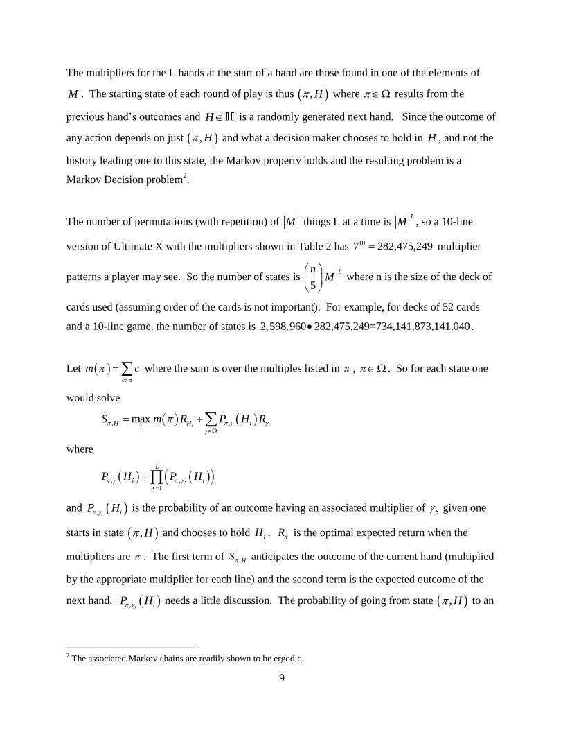
In multi-line versions, the outcome of each line establishes the multiplier for the next hand on
that line. Figure 1 shows the game after a hand has established multipliers. Here the multiplier
on the second hand was 2 at the start of play and zero for the other two hands. Two deuces were
held. The completion resulted in outcomes of a four of a kind on hand one (giving a multiplier
of 7 for the next hand on this line), and three of a kinds on the other two hands (giving
multipliers for the next hands of 2). The payout on this hand was the regular payout for the three
of a kind (1), plus two times the payout for a three of a kind, plus the regular payout for a four of
a kind (4) giving a total of 7 (times the number of bet units played).

8
Figure 1: 3-line deuces wild Ultimate X Poker (http://www.videopoker.com/)
An analysis of this game is substantially more involved than the typical video poker game since
the current hand’s return depends on the outcome of the previous hand. This note provides an
analysis of the game. To our knowledge, this game had not been rigorously analyzed. A
leading expert on gambling analyses, Michael Shackleford, states while referring to tables of
expected returns of the various forms of the Ultimate X game:
―This would have been a very difficult analysis, and nobody would have cared, other than
me, if I cracked it. So the above tables have been kindly provided by IGT (the game
maker), who I thank. All I know is that they did an "exhaustive" analysis, meaning they
looked at the billions of possible game states to arrive at a return‖
(http://wizardofodds.com/ultimatex Shackleford 2010).
Just what type of analysis IGT performed was not reported. As it turns out, our analysis
confirms the IGT values, so they obviously performed a rigorous analysis. Nonetheless, their
work is unpublished and this paper makes clear the challenges of analyzing this game and leaves
open several interesting avenues for future research.
2. Analysis of Ultimate X Poker
Let L be the number of lines played. Let M be the set of possible payoff multipliers. For
example, in Table 2, 1,2,3,4,5,7,12M . Let be the set of permutations of the elements of
M taken L at a time with repetition. For example, for 2L
1,1 , 1,2 , 1,3 , 1,4 , 1,5 , 1,7 , 1,12 , 2,1 , , 12,12 .
9
The multipliers for the L hands at the start of a hand are those found in one of the elements of
M . The starting state of each round of play is thus , H where results from the
previous hand’s outcomes and H is a randomly generated next hand. Since the outcome of
any action depends on just , H and what a decision maker chooses to hold in H , and not the
history leading one to this state, the Markov property holds and the resulting problem is a
Markov Decision problem2.
The number of permutations (with repetition) of M things L at a time is L
M , so a 10-line
version of Ultimate X with the multipliers shown in Table 2 has 107 282,475,249 multiplier
patterns a player may see. So the number of states is 5
LnM
where n is the size of the deck of
cards used (assuming order of the cards is not important). For example, for decks of 52 cards
and a 10-line game, the number of states is 2,598,960 282,475,249=734,141,873,141,040 .
Let c
m c
where the sum is over the multiples listed in , . So for each state one
would solve
, ,maxiH H i
iS m R P H R
where
, ,
1
L
i iP H P H
and , iP H is the probability of an outcome having an associated multiplier of given one
starts in state , H and chooses to hold iH . R is the optimal expected return when the
multipliers are . The first term of ,HS anticipates the outcome of the current hand (multiplied
by the appropriate multiplier for each line) and the second term is the expected outcome of the
next hand. , iP H needs a little discussion. The probability of going from state , H to an
2 The associated Markov chains are readily shown to be ergodic.

10
outcome having an associated multiplier of is dependent only on iH , not on . Of course,
an optimal choice for subset i does depend on , and we use our notation to reflect this.
Since the present decision impacts future returns and decisions, several considerations are
possible. If the time-value of money plays a role (for example, a professional gambler may play
the game over a period of months or years), then one might discount the returns from future
hands by focusing on the following problem
,maxiH i
im R P H R
.
Here 0,1 is a discount factor giving the expected present value of money from the next
decision period. Since the game play is quick, it is hard to imagine that would be measurably
smaller than 1.0 so, more commonly, one would probably not discount the future returns. In
such cases a non-discounted form of the problem is appropriate.
Another factor is the length of play. Although there will always be only a finite number of
rounds of play, the mathematical analysis and long-term results are best handled by assuming an
infinite number of rounds of play. This not only simplifies the calculations but gives strategies
that are optimal for assuming a reasonable number of rounds are played. For the non-discounted
problem this can result in infinite (negate or positive) total returns. So, for the non-discounted
case, one focuses on maximizing the average gain per round of play (e.g., see Derman 1970).
The infinite horizon, non-discounted, Markov Decision problem (ndMDP) for this game is stated
as
,max
0
iH ii
H
v g m R P H v
P v
(1)
where g is the maximal gain per round of play and P is the steady-state probability of being in
state (before a hand is dealt) under optimal decisions. The value v is interpreted as the
relative bias for state . Note that g KL is the optimal expected return per bet unit for
the game.

11
An ndMDP is usually solved using one of three methods: value iteration, policy iteration or
linear programming (for example, see Derman, 1970). All of these methods are computationally
sensitive to the number of states involved, which, as shown above, could be very large. Both
linear programming and policy improvement methods would require enormous numbers of
equations and are not practical alternatives since both would require working with items (e.g.,
matrices) having a size equal to at least the square of the number of states, truly large sizes.
Value iteration offers an advantage in that one needs only essentially four vectors the size of the
(two for the relative biases v and two for the stationary probabilities P ). Indeed, there are
value iteration methods needing only two such vectors (where Gauss-Seidel iterations are used
e.g., Porteus 1981).
We studied this problem using value-iteration (Derman 1970). With value iteration one
successively solves
1 1
,maxi
n n n
H ii
H
v g m R P H v
(2)
1 1 1n n ng P v
,
1
, H
n n
i SP P P H
These iterations continue until the change in iterates (1 1 1, ,n n nv g P
) reduces to some small
value. It is well-known that these converge. For a one line version of the Ultimate X Poker game
in Table 2 we found the results shown in Table 3. The optimal gain rate is 1.989680522g
making it a negative expected value game (since 2K ). Its expected return per unit bet is
0.994840.
Deuces Wild – 1 Line
v P
(1) -1.003399219 0.556280413
(2) -0.01819477 0.265939238
(3) 0.968865825 0.058338112
(4) 1.956764857 0.001788994

12
(5) 2.945128634 0.051826156
(7) 4.922771038 0.060508713
(12) 9.868120983 0.005318374
Table 3: Solution to one line version of the game with multiples in Table 2
To proceed much beyond one line games, some algorithmic tricks are needed because the
problem sizes grow so fast. Now, many of the states, , are equivalent in terms of a
player’s expected return and the transition probabilities to subsequent states. We discussed
earlier how the outcomes of many hands are equivalent to other hands where the suites have been
permuted. Likewise, many of the multiplier permutations are equivalent. For example, in a 3-
line game, 3,5,5 will give the same expected payouts as 5,3,5 and 5,5,3 . Clearly the
order of the multipliers across the lines of play is not important. Let C contain just the
unique combinations (say those in sorted order). So
1
1
M LC
M
.
Hence, one can focus on just C payoff patterns (i.e., the number of combinations with
repetition), recognizing that some may have multiple different ways they can be seen. Thus, for
a ten-line game, one can reduce the state space size to
16
134,459 1,076,747,6726
C
states. This is clearly better than the 147.34 10 states shown earlier, but is still a large number.
With this, we can reduce (2) in a straightforward manner. Before doing so, another reduction
results from the following theorem. This insight was first noted by Shackleford
(http://wizardofodds.com/ultimatex Shackleford 2010) where he states:
―The strategy in Ultimate X will depend not only on your cards, but the sum of the
current multipliers.‖

13
Theorem 1
Let , then R R if m m .
Proof:
Solutions satisfy (1) so
,maxiH i
iH
R g m R P H R
,maxiH i
iH
R g m R P H R
and then
,
,
max
max
i
i
H ii
H
H ii
H
m R P H R
R R
m R P H R
, ,
, ,, ,
i S i SH H
H H
H H
H i S i S
m R m R
P H R P H R
.
But, by assumption, m m so we get this last term reduces to
, ,, ,H Hi S i S
H
P H P H R R
.
Likewise
, ,, ,H Hi S i S
H
R R P H P H R R
.
However, as discussed earlier, , ,i iP H P H so we have 0 0R R .
Thus the computational burden can be reduced further to considering just representative
combinations in C for each possible sum m . Let D C be such a set. For example,
for the multipliers in Table 2 the differences in state sizes are shown in Table 4.

14
3-Lines 5-Lines 10-Lines
343 16,807 282,475,249
C 84 462 8,008
D 29 51 106
Table 4: Size of Sets
Then the first line of (2) can be reduced to
1 1
,maxi
n n n
H ii
H D
v g m R P H v D
(3)
1 1 / ,n nv v D m m
where
, ,i i
m m
P H P H
Of course, the first line can be reduced further to
1 1
,maxi
n n n
H ii
H D
v g f H m R P H v D
(4)
1 1 / ,n nv v D m m .
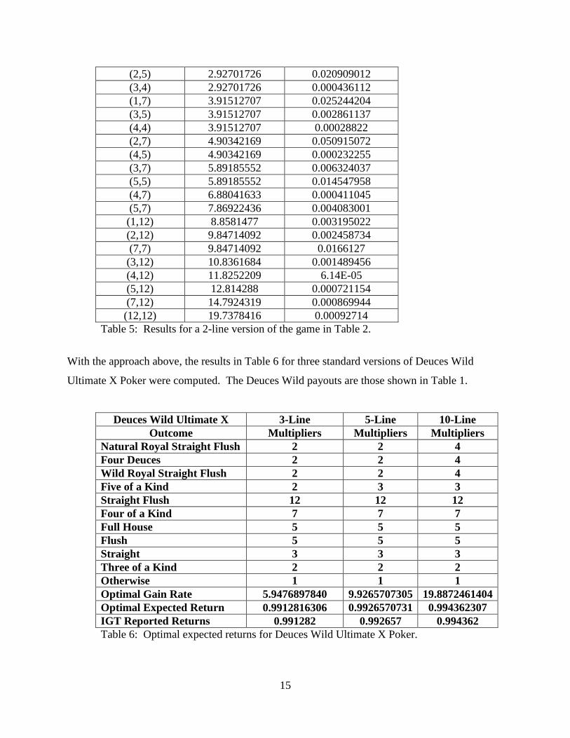
Using this approach we found the results shown in Table 5 for a 2-line version of the game with
multipliers in Table 2. The optimal gain rate is 3.978525287g . The expected return per unit
bet is 0.994631.
Deuces Wild – 2 Lines
D v P
(1,1) -2.0052132 0.392717712
(1,2) -1.0209311 0.207469421
(1,3) -0.0347993 0.044863041
(2,2) -0.0347993 0.114908538
(1,4) 0.95206921 0.001048511
(2,3) 0.95206921 0.019711084
(1,5) 1.9393246 0.045285236
(2,4) 1.9393246 0.000842345
(3,3) 1.9393246 0.02056649
15
(2,5) 2.92701726 0.020909012
(3,4) 2.92701726 0.000436112
(1,7) 3.91512707 0.025244204
(3,5) 3.91512707 0.002861137
(4,4) 3.91512707 0.00028822
(2,7) 4.90342169 0.050915072
(4,5) 4.90342169 0.000232255
(3,7) 5.89185552 0.006324037
(5,5) 5.89185552 0.014547958
(4,7) 6.88041633 0.000411045
(5,7) 7.86922436 0.004083001
(1,12) 8.8581477 0.003195022
(2,12) 9.84714092 0.002458734
(7,7) 9.84714092 0.0166127
(3,12) 10.8361684 0.001489456
(4,12) 11.8252209 6.14E-05
(5,12) 12.814288 0.000721154
(7,12) 14.7924319 0.000869944
(12,12) 19.7378416 0.00092714
Table 5: Results for a 2-line version of the game in Table 2.
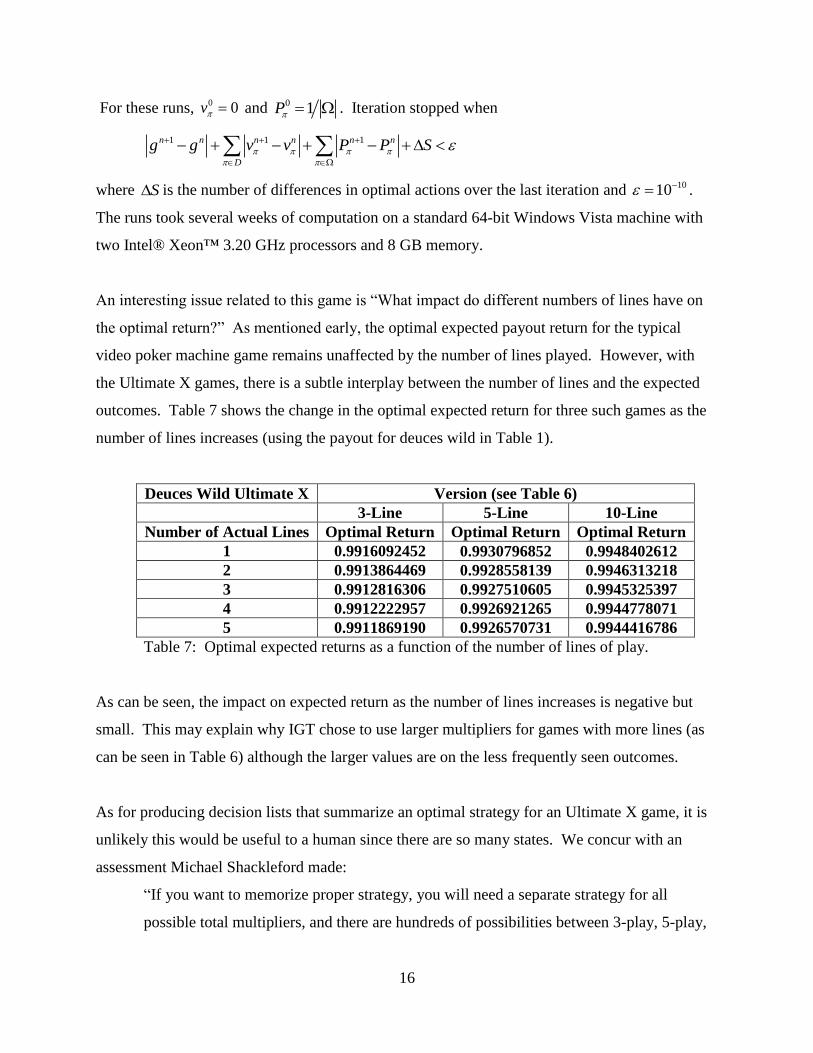
With the approach above, the results in Table 6 for three standard versions of Deuces Wild
Ultimate X Poker were computed. The Deuces Wild payouts are those shown in Table 1.
Deuces Wild Ultimate X
Video Poker
3-Line 5-Line 10-Line
Outcome Multipliers Multipliers Multipliers
Natural Royal Straight Flush 2 2 4
Four Deuces 2 2 4
Wild Royal Straight Flush 2 2 4
Five of a Kind 2 3 3
Straight Flush 12 12 12
Four of a Kind 7 7 7
Full House 5 5 5
Flush 5 5 5
Straight 3 3 3
Three of a Kind 2 2 2
Otherwise 1 1 1
Optimal Gain Rate 5.9476897840 9.9265707305 19.8872461404
Optimal Expected Return 0.9912816306 0.9926570731 0.994362307
IGT Reported Returns 0.991282 0.992657 0.994362
Table 6: Optimal expected returns for Deuces Wild Ultimate X Poker.
16
For these runs, 0 0v and 0 1P . Iteration stopped when
1 1 1n n n n n n
D
g g v v P P S
where S is the number of differences in optimal actions over the last iteration and 1010 .
The runs took several weeks of computation on a standard 64-bit Windows Vista machine with
two Intel® Xeon™ 3.20 GHz processors and 8 GB memory.
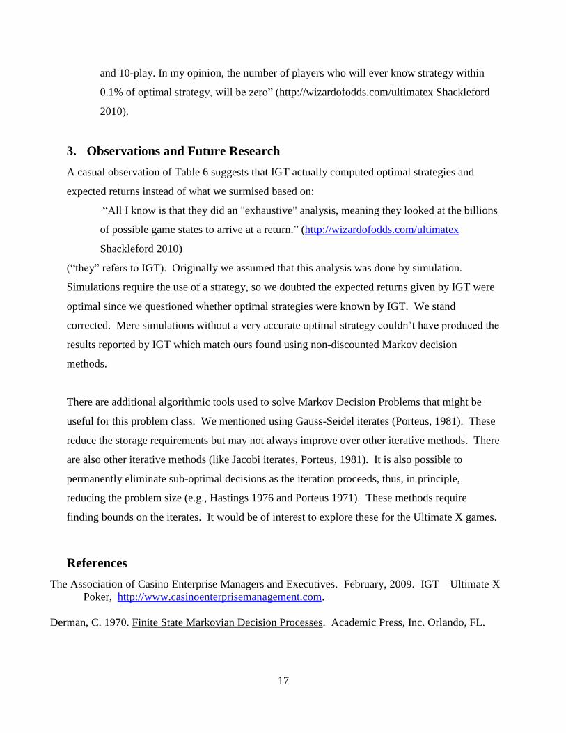
An interesting issue related to this game is ―What impact do different numbers of lines have on
the optimal return?‖ As mentioned early, the optimal expected payout return for the typical
video poker machine game remains unaffected by the number of lines played. However, with
the Ultimate X games, there is a subtle interplay between the number of lines and the expected
outcomes. Table 7 shows the change in the optimal expected return for three such games as the
number of lines increases (using the payout for deuces wild in Table 1).
Deuces Wild Ultimate X
Video Poker
Version (see Table 6)
3-Line
5-Line 10-Line
Number of Actual Lines Optimal Return Optimal Return Optimal Return
1 0.9916092452 0.9930796852 0.9948402612
2 0.9913864469 0.9928558139 0.9946313218
3 0.9912816306 0.9927510605 0.9945325397
4 0.9912222957 0.9926921265 0.9944778071
5 0.9911869190 0.9926570731 0.9944416786
Table 7: Optimal expected returns as a function of the number of lines of play.
As can be seen, the impact on expected return as the number of lines increases is negative but
small. This may explain why IGT chose to use larger multipliers for games with more lines (as
can be seen in Table 6) although the larger values are on the less frequently seen outcomes.
As for producing decision lists that summarize an optimal strategy for an Ultimate X game, it is
unlikely this would be useful to a human since there are so many states. We concur with an
assessment Michael Shackleford made:
―If you want to memorize proper strategy, you will need a separate strategy for all
possible total multipliers, and there are hundreds of possibilities between 3-play, 5-play,
17
and 10-play. In my opinion, the number of players who will ever know strategy within
0.1% of optimal strategy, will be zero‖ (http://wizardofodds.com/ultimatex Shackleford
2010).
3. Observations and Future Research
A casual observation of Table 6 suggests that IGT actually computed optimal strategies and
expected returns instead of what we surmised based on:
―All I know is that they did an "exhaustive" analysis, meaning they looked at the billions
of possible game states to arrive at a return.‖ (http://wizardofodds.com/ultimatex
Shackleford 2010)
(―they‖ refers to IGT). Originally we assumed that this analysis was done by simulation.
Simulations require the use of a strategy, so we doubted the expected returns given by IGT were
optimal since we questioned whether optimal strategies were known by IGT. We stand
corrected. Mere simulations without a very accurate optimal strategy couldn’t have produced the
results reported by IGT which match ours found using non-discounted Markov decision
methods.
There are additional algorithmic tools used to solve Markov Decision Problems that might be
useful for this problem class. We mentioned using Gauss-Seidel iterates (Porteus, 1981). These
reduce the storage requirements but may not always improve over other iterative methods. There
are also other iterative methods (like Jacobi iterates, Porteus, 1981). It is also possible to
permanently eliminate sub-optimal decisions as the iteration proceeds, thus, in principle,
reducing the problem size (e.g., Hastings 1976 and Porteus 1971). These methods require
finding bounds on the iterates. It would be of interest to explore these for the Ultimate X games.
References
The Association of Casino Enterprise Managers and Executives. February, 2009. IGT—Ultimate X
Poker, http://www.casinoenterprisemanagement.com.
Derman, C. 1970. Finite State Markovian Decision Processes. Academic Press, Inc. Orlando, FL.
18
Hastings, N. A. J. 1976. Test for Nonoptimal Actions in Undiscounted Finite Markov Decision
Chains. Management Science, Vol. 23, No. 1, pp. 87-92.
Porteus, E. L. 1981. Computing the Discounted Return in Markov and Semi-Markov Chains.
Naval Research Logistics Quarterly, Volume 28 Issue 4, Pages 567 – 577.
Porteus, E. L. 1971. Some Bounds for Discounted Sequential Decision Processes. Management
Science, 18, No. l, pp. 7-11.
Quinlan, J. R. C4.5: Programs for Machine Learning. Morgan Kaufmann Publishers, 1993.
Rivest, R. 1987. Learning Decision Lists. Machine Learning, 2, No. 3, pp. 229-246.
Shackleford, M. 2010. The Wizard of Odds Web Site, http://wizardofodds.com/.