UL Winter School Quantitative Stream Unit B2: …teaching.sociology.ul.ie/ws/wsCatDatsl8.pdfUL Winter School Quantitative Stream Unit B2: Categorical Data Analysis ... 6 UL Winter

sociologyAT UNIVERSITY OF LIMERICK

UNIVERSITY OF LIMERICKsociology




UL Winter School Quantitative Stream Unit B2: Categorical Data Analysis

UL Winter School Quantitative StreamUnit B2: Categorical Data Analysis

Brendan HalpinDepartment of SociologyUniversity of Limerick

[email protected]

January 16–18, 2017

1







Outline

1 Association in tables

2 Logistic regression

3 Extensions to multinomial, ordinal regression

4 Multinomial logistic regression

5 Ordinal logit

6 Special topics: depending on interest

2







Overview

Overview

This 3-day section focuses on categorical dataAnalysis of data in tables, association between categoricalvariablesLogistic regression: regression with a binary variable asdependentExtensions of logistic regression – multinomial, ordinal.Draws heavily on Chs 8 (part) and 15 of Agresti & Finlay

3






UL Winter School Quantitative Stream Unit B2: Categorical Data AnalysisAssociation in tables

Outline





5 Ordinal logit


4






UL Winter School Quantitative Stream Unit B2: Categorical Data AnalysisAssociation in tablesAssociation in tables

Association in tables

Tables display association between categorical variablesMade evident by patterns of percentagesTested by χ2 test

5







Association

How do we characterise association?Is there association?What form does it take?How strong is it?

6







Is there association?

This is what the χ2 test determines – evidence of associationDoes not characterise nature or size!Depends on NOther tests exist, such as Fisher’s exact test

7







What form does it take?

Examine percentagesCompare observed and expected: residualsStandardised residuals: behave like z , i.e., should lie in range−2 : +2 about 95% of time, if independence is true

z = O−E√E(1−row proportion)(1−col proportion)

= O−E√E(1− R

T)(1− C

T)

8







How strong is it?

Many possible measures of associationDifference in proportionsRatio of proportions or “relative rate”Ratio of odds or “odds ratio”

(see http://teaching.sociology.ul.ie:3838/apps/orrr/)

9







Ordinal variables

Ordinal variables may have more structured associationSimpler pattern, analogous to correlationX high, Y high; X low, Y low

10







Characterising ordinal association

Focus on concordant/discordant pairsPairs of cases which differ on both variables

Concordant: case that is higher on one variable also higher onotherDiscordant: higher on one, lower on the other

Gamma, γ̂ = C−DC+D

Values range −1 ≤ γ ≤ +1like correlation in interpretationHas asymptotic standard error ⇒ t-test possible

11







Higher order tables

We can consider association in higher-order tables, e.g., 3-wayIs the association between A and B the same for differentvalues of C?Does the association between A and B dissapear if we controlfor C?

12







Simpson’s paradox etc.

Scouting example (ch 10): negative association betweenscouting and delinquencyControl for family characteristics (church attendance) and itdisappearsSee also death penalty example: note pattern of odds ratiosCochran-Mantel-Haenszel test: 2× 2× k tableH0 : within each of k 2× 2 panels, OR = 1

13







Scouting 1/3

| delinqscout | 0 1 | Total

-----------+----------------------+----------0 | 36 364 | 4001 | 60 340 | 400

-----------+----------------------+----------Total | 96 704 | 800

14







Scouting 2/3

--------------------------------------------------| church and delinq| ---- 0 --- ---- 1 --- ---- 2 ---

scout | 0 1 0 1 0 1----------+---------------------------------------

0 | 10 40 18 132 8 1921 | 40 160 18 132 2 48

--------------------------------------------------

15







Scouting 3/3

| churchscout | 0 1 2 | Total

-----------+---------------------------------+----------0 | 50 150 200 | 4001 | 200 150 50 | 400

-----------+---------------------------------+----------Total | 250 300 250 | 800

16







Loglinear modelling

More complex questions and larger tables can be handled byloglinear modellingTreats all variables as “dependent variables”Can test null hypothesis of independence, as well as specifiedpatterns of interaction

17






UL Winter School Quantitative Stream Unit B2: Categorical Data AnalysisLogistic regression

Outline





5 Ordinal logit


18






UL Winter School Quantitative Stream Unit B2: Categorical Data AnalysisLogistic regressionLogistic regression

Logistic regression

OLS regression requires interval dependent variableBinary or “yes/no” dependent variables are not suitableNor are rates, e.g., n successes out of m trialsErrors are distinctly not normalWhile predicted value can be read as a probability, can departfrom 0:1 rangeParticular difficulties with multiple explanatory variables.

19







Linear Probability Model

OLS gives the “linear probability model” in this case:

Pr(Y = 1) = a+ bX

data is 0/1, prediction is probabilityAssumptions violated, but if predicted probabilities in range0.2–0.8, not too badSee credit card example: becomes unrealistic only at very lowor high income

20







Logistic transformation

Probability is bounded [0 : 1]OLS predicted value is unboundedHow to transform probability to −∞ :∞ range?Odds: p

1−p – range is 0 :∞Log of odds: log p

1−p has range −∞ :∞

21







Logistic regression

Logistic regression uses this as the dependent variable:

log(

Pr(Y = 1)1− Pr(Y = 1)

)= a+ bX

Alternatively:

Pr(Y = 1)1− Pr(Y = 1)

= ea+bX

Or:

Pr(Y = 1) =ea+bX

1+ ea+bX=

11+ e−a−bX

22







Parameters

The b parameter is the effect of a unit change in X onlog(

Pr(Y=1)1−Pr(Y=1)

)

This implies a multiplicative change of eb in Pr(Y=1)1−Pr(Y=1) , in the

OddsThus an odds ratioBut the effect of b on P depends on the level of bSee credit card exampleDeath penalty example allows us to see the link between oddsratios and estimates

23






UL Winter School Quantitative Stream Unit B2: Categorical Data AnalysisLogistic regressionInference

Inference

In practice, inference is similar to OLS though based on adifferent logicFor each explanatory variable, H0 : β = 0 is the interesting null

z = β̂SE is approximately normally distributed (large sample

property)

More usually, the Wald test is used:(β̂SE

)2has a χ2

distribution with one degree of freedom

24







Likelihood ratio tests

The “likelihood ratio” test is thought more robust than theWald test for smaller samplesWhere l0 is the likelihood of the model without Xj , and l1 thatwith it, the quantity

−2(log

l0l1

)= −2 (log l0 − log l1)

is χ2 distributed with one degree of freedom

25







Nested models

More generally, −2(log lo

l1

)tests nested models: where model

1 contains all the variables in model 0, plus m extra ones, ittests the null that all the extra $β$s are zero (χ2 with m df)If we compare a model against the null model (no explanatoryvariables, it tests

H0 : β1 = β2 = . . . = βk = 0

Strong analogy with F -test in OLS

26






UL Winter School Quantitative Stream Unit B2: Categorical Data AnalysisLogistic regressionMaximum likelihood

Maximum likelihood estimation

What is this “likelihood”?Unlike OLS, logistic regression (and many, many other models)are extimated by maximum likelihood estimationIn general this works by choosing values for the parameterestimates which maximise the probability (likelihood) ofobserving the actual dataOLS can be ML estimated, and yields exactly the same results

27







Iterative search

Sometimes the values can be chosen analyticallyA likelihood function is written, defining the probability ofobserving the actual data given parameter estimatesDifferential calculus derives the values of the parameters thatmaximise the likelihood, for a given data set

Often, such “closed form solutions” are not possible, and thevalues for the parameters are chosen by a systematiccomputerised search (multiple iterations)Extremely flexible, allows estimation of a vast range ofcomplex models within a single framework

28







Likelihood as a quantity

Either way, a given model yields a specific maximum likelihoodfor a give data setThis is a probability, henced bounded [$0:1$]Reported as log-likelihood, hence bounded [$-∞:0$]Thus is usually a large negative numberWhere an iterative solution is used, likelihood at each stage isusually reported – normally getting nearer 0 at each step

29






UL Winter School Quantitative Stream Unit B2: Categorical Data AnalysisLogistic regressionTabular data

Tabular data

If all the explanatory variables are categorical (or have fewfixed values) your data set can be represented as a tableIf we think of it as a table where each cell contains n yeses andm − n noes (n successes out of m trials) we can fit groupedlogistic regressionn successes out of m trials implies a binomial distribution ofdegree m

logn

m − n= α+ βX

The parameter estimates will be exactly the same as if thedata were treated individually

30






UL Winter School Quantitative Stream Unit B2: Categorical Data AnalysisLogistic regressionTabular data

Tabular data and goodness of fit

But unlike with individual data, we can calculate goodness offit, by relating observed successes to predicted in each cellIf these are close we cannot reject the null hypothesis that themodel is incorrect (i.e., you want a high p-value)Where li is the likelihood of the current model, and ls is thelikelihood of the “saturated model” the test statistic is

−2(log

lils

)

The saturated model predicts perfectly and has as manyparameters as there are “settings” (cells in the table)The test has df of number of settings less number ofparameters estimated, and is χ2 distributed

31






UL Winter School Quantitative Stream Unit B2: Categorical Data AnalysisLogistic regressionGoodness of fit and accuracy of classification

Fit with individual data

Where the number of “settings” (combinations of values ofexplanatory variables) is large, this approach to fit is notfeasibleCannot be used with continuous covariatesHosmer-Lemeshow statistic attempts to create an analogy

Divide sample into deciles of predicted probabilityCalculate a fit measure based on observed and predictednumbers in the ten groupsSimulation shows this is χ2 distributed with 2 dfNot a perfect solution, sensitive to how the cuts are made

Pseudo-R2 measures exist, but none approaches the cleaninterpretation as in OLSSee http://www.ats.ucla.edu/stat/mult_pkg/faq/general/Psuedo_RSquareds.htm

32







Predicting outcomes

Another way of assessing the adequacy of a logit model is itsaccuracy of classification:

True yes True no

Predicted yes a c

Predicted no b d

Proportion correctly classified: a+da+b+c+d

Sensitivity: aa+b ; Specificity:

dc+d

False positive: ca+c ; False negative: b

b+d

Stata: estat class

33







Some problems

Zero cells in tables can cause problems: no yeses or no noesfor particular settingsNot automatically a problem but can give rise to attempts toestimate a parameter as −∞ or +∞If this happens, you will see a large parameter estimate and ahuge standard errorIn individual data, sometimes certain combinations of variableshave only successes or only failuresIn Stata, these cases are dropped from estimation – you needto be aware of this as it changes the interpretation (you maywish to drop one of the offending variables instead)

34






UL Winter School Quantitative Stream Unit B2: Categorical Data AnalysisExtensions to multinomial, ordinal regression

Outline





5 Ordinal logit


35






UL Winter School Quantitative Stream Unit B2: Categorical Data AnalysisMultinomial logistic regression

Outline





5 Ordinal logit


36






UL Winter School Quantitative Stream Unit B2: Categorical Data AnalysisMultinomial logistic regressionbaseline category extension of binary

What if we have multiple possible outcomes, not justtwo?

Logistic regression is binary: yes/noMany interesting dependent variables have multiple categories

voting intention by partyfirst destination after second-level educationhousing tenure type

We can use binary logistic byrecoding into two categoriesdropping all but two categories

But that would lose information

37







Multinomial logistic regression

Another idea:Pick one of the J categories as baselineFor each of J − 1 other categories, fit binary modelscontrasting that category with baselineMultinomial logistic effectively does that, fitting J − 1 modelssimultaneously

logP(Y = j)

P(Y = J)= αj + βjX , j = 1, . . . , c − 1

Which category is baseline is not critically important, butbetter for interpretation if it is reasonably large and coherent(i.e. "Other" is a poor choice)

38







Predicting p from formula

logπjπJ

= αj + βjX

πjπJ

= eαj+βjX

πj = πJeαj+βjX

πJ = 1−J−1∑

k=1

πk = 1− πJJ−1∑

k=1

eαk+βkX

πJ =1

1+∑J−1

k=1 eαk+βkX

=1

∑Jk=1 e

αk+βkX

⇒ πj =eαj+βjX

∑Jk=1 e

αk+βkX

39






UL Winter School Quantitative Stream Unit B2: Categorical Data AnalysisMultinomial logistic regressionInterpreting example, inference

Example

Let’s attempt to predict housing tenureOwner occupierLocal authority renterPrivate renter

using age and employment statusEmployedUnemployedNot in labour force

mlogit ten3 age i.eun

40







Stata output

Multinomial logistic regression Number of obs = 15490LR chi2(6) = 1256.51Prob > chi2 = 0.0000

Log likelihood = -10204.575 Pseudo R2 = 0.0580

------------------------------------------------------------------------------ten3 | Coef. Std. Err. z P>|z| [95% Conf. Interval]

-------------+----------------------------------------------------------------1 | (base outcome)-------------+----------------------------------------------------------------2 |

age | -.0103121 .0012577 -8.20 0.000 -.012777 -.0078471|

eun |2 | 1.990774 .1026404 19.40 0.000 1.789603 2.1919463 | 1.25075 .0522691 23.93 0.000 1.148304 1.353195

|_cons | -1.813314 .0621613 -29.17 0.000 -1.935148 -1.69148

-------------+----------------------------------------------------------------3 |

age | -.0389969 .0018355 -21.25 0.000 -.0425945 -.0353994|

eun |2 | .4677734 .1594678 2.93 0.003 .1552223 .78032453 | .4632419 .063764 7.26 0.000 .3382668 .5882171

|_cons | -.76724 .0758172 -10.12 0.000 -.915839 -.6186411

------------------------------------------------------------------------------

41







Interpretation

Stata chooses category 1 (owner) as baselineEach panel is similar in interpretation to a binary regression onthat category versus baselineEffects are on the log of the odds of being in category j versusthe baseline

42







Inference

At one level inference is the same:Wald test for Ho : βk = 0LR test between nested models

However, each variable has J − 1 parametersBetter to consider the LR test for dropping the variable acrossall contrasts: H0 : ∀ j : βjk = 0Thus retain a variable even for contrasts where it isinsignificant as long as it has an effect overallWhich category is baseline affects the parameter estimates butnot the fit (log-likelihood, predicted values, LR test onvariables)

43






UL Winter School Quantitative Stream Unit B2: Categorical Data AnalysisOrdinal logit

Outline





5 Ordinal logit


44






UL Winter School Quantitative Stream Unit B2: Categorical Data AnalysisOrdinal logit

Predicting ordinal outcomes

While mlogit is attractive for multi-category outcomes, it isimparsimoniousFor nominal variables this is necessary, but for ordinal variablesthere should be a better wayWe consider three useful models

Stereotype logitProportional odds logitContinuation ratio or sequential logit

Each approaches the problem is a different way

45






UL Winter School Quantitative Stream Unit B2: Categorical Data AnalysisOrdinal logitStereotype logit

Stereotype logit

If outcome is ordinal we should see a pattern in the parameterestimates:

. mlogit educ c.age i.sex if age>30[...]Multinomial logistic regression Number of obs = 10905

LR chi2(4) = 1171.90Prob > chi2 = 0.0000


------------------------------------------------------------------------------educ | Coef. Std. Err. z P>|z| [95% Conf. Interval]

-------------+----------------------------------------------------------------Hi |

age | -.0453534 .0015199 -29.84 0.000 -.0483323 -.04237442.sex | -.4350524 .0429147 -10.14 0.000 -.5191636 -.3509411_cons | 2.503877 .086875 28.82 0.000 2.333605 2.674149

-------------+----------------------------------------------------------------Med |

age | -.0380206 .0023874 -15.93 0.000 -.0426999 -.03334132.sex | -.1285718 .0674878 -1.91 0.057 -.2608455 .0037019_cons | .5817336 .1335183 4.36 0.000 .3200425 .8434246

-------------+----------------------------------------------------------------Lo | (base outcome)------------------------------------------------------------------------------

46







Ordered parameter estimates

Low education is the baselineThe effect of age:

-0.045 for high vs low-0.038 for medium vs low0.000, implicitly for low vs low

Sex: -0.435, -0.129 and 0.000Stereotype logit fits a scale factor φ to the parameterestimates to capture this pattern

47







Scale factor

Compare mlogit:

logP(Y = j)

P(Y = J)= αj + β1jX1 + β2jX, j = 1, . . . , J − 1

with slogit

logP(Y = j)

P(Y = J)= αj + φjβ1X1 + φjβ2X2, j = 1, . . . , J − 1

φ is zero for the baseline category, and 1 for the maximumIt won’t necessarily rank your categories in the right order:sometimes the effects of other variables do not coincide withhow you see the ordinality

48







Slogit example

. slogit educ age i.sex if age>30[...]Stereotype logistic regression Number of obs = 10905

Wald chi2(2) = 970.21Log likelihood = -9784.863 Prob > chi2 = 0.0000

( 1) [phi1_1]_cons = 1------------------------------------------------------------------------------

educ | Coef. Std. Err. z P>|z| [95% Conf. Interval]-------------+----------------------------------------------------------------

age | .0457061 .0015099 30.27 0.000 .0427468 .04866542.sex | .4090173 .0427624 9.56 0.000 .3252045 .4928301

-------------+----------------------------------------------------------------/phi1_1 | 1 (constrained)/phi1_2 | .7857325 .0491519 15.99 0.000 .6893965 .8820684/phi1_3 | 0 (base outcome)

-------------+----------------------------------------------------------------/theta1 | 2.508265 .0869764 28.84 0.000 2.337795 2.678736/theta2 | .5809221 .133082 4.37 0.000 .3200862 .841758/theta3 | 0 (base outcome)

------------------------------------------------------------------------------(educ=Lo is the base outcome)

49







Interpreting φ

With low education as the baseline, we find φ estimates thus:

High 1Medium 0.786Low 0

That is, averaging across the variables, the effect of mediumvs low is 0.786 times that of high vs lowThe /theta terms are the αjs

50







Surprises from slogit

slogit is not guaranteed to respect the order

Stereotype logistic regression Number of obs = 14321Wald chi2(2) = 489.72

Log likelihood = -13792.05 Prob > chi2 = 0.0000

( 1) [phi1_1]_cons = 1------------------------------------------------------------------------------


age | .0219661 .0009933 22.11 0.000 .0200192 .02391292.sex | .1450657 .0287461 5.05 0.000 .0887244 .2014071

-------------+----------------------------------------------------------------/phi1_1 | 1 (constrained)/phi1_2 | 1.813979 .0916542 19.79 0.000 1.634341 1.993618/phi1_3 | 0 (base outcome)

-------------+----------------------------------------------------------------/theta1 | .9920811 .0559998 17.72 0.000 .8823235 1.101839/theta2 | .7037589 .0735806 9.56 0.000 .5595436 .8479743/theta3 | 0 (base outcome)


age has a strongly non-linear effect and changes the order of φ

51







Recover by including non-linear age

Stereotype logistic regression Number of obs = 14321Wald chi2(3) = 984.66

Log likelihood = -13581.046 Prob > chi2 = 0.0000

( 1) [phi1_1]_cons = 1------------------------------------------------------------------------------


age | -.1275568 .0071248 -17.90 0.000 -.1415212 -.1135924|

c.age#c.age | .0015888 .0000731 21.74 0.000 .0014456 .0017321|

2.sex | .3161976 .0380102 8.32 0.000 .2416989 .3906963-------------+----------------------------------------------------------------

/phi1_1 | 1 (constrained)/phi1_2 | .5539747 .0479035 11.56 0.000 .4600854 .6478639/phi1_3 | 0 (base outcome)

-------------+----------------------------------------------------------------/theta1 | -1.948551 .1581395 -12.32 0.000 -2.258499 -1.638604/theta2 | -2.154373 .078911 -27.30 0.000 -2.309036 -1.999711/theta3 | 0 (base outcome)


52







Stereotype logit

Stereotype logit treats ordinality as ordinality in terms of theexplanatory variablesThere can be therefore disagreements between variables aboutthe pattern of ordinalityIt can be extended to more dimensions, which makes sense forcategorical variables whose categories can be thought of asarrayed across more than one dimensionSee Long and Freese, Ch 6.8

53






UL Winter School Quantitative Stream Unit B2: Categorical Data AnalysisOrdinal logitProportional odds

The proportional odds model

The most commonly used ordinal logistic model has anotherlogicIt assumes the ordinal variable is based on an unobservedlatent variableUnobserved cutpoints divide the latent variable into the groupsindexed by the observed ordinal variableThe model estimates the effects on the log of the odds ofbeing higher rather than lower across the cutpoints

54







The model

For j = 1 to J − 1,

logP(Y > j)

P(Y <= j)= αj + βx

Only one β per variable, whose interpretation is the effect onthe odds of being higher rather than lowerOne α per contrast, taking account of the fact that there aredifferent proportions in each one

55







J − 1 contrasts again, but different

But rather thancomparecategoriesagainst abaseline it splitsinto high andlow, with all thedata involvedeach time

56







An example

Using data from the BHPS, we predict the probability of eachof 5 ordered responses to the assertion "homosexualrelationships are wrong"Answers from 1: strongly agree, to 5: strongly disagreeSex and age as predictors – descriptively women and youngerpeople are more likely to disagree (i.e., have high values)

57







Ordered logistic: Stata output

Ordered logistic regression Number of obs = 12725LR chi2(2) = 2244.14Prob > chi2 = 0.0000


------------------------------------------------------------------------------ropfamr | Coef. Std. Err. z P>|z| [95% Conf. Interval]

-------------+----------------------------------------------------------------2.rsex | .8339045 .033062 25.22 0.000 .7691041 .8987048

rage | -.0371618 .0009172 -40.51 0.000 -.0389595 -.035364-------------+----------------------------------------------------------------

/cut1 | -3.833869 .0597563 -3.950989 -3.716749/cut2 | -2.913506 .0547271 -3.02077 -2.806243/cut3 | -1.132863 .0488522 -1.228612 -1.037115/cut4 | .3371151 .0482232 .2425994 .4316307

------------------------------------------------------------------------------

58







Interpretation

The betas are straightforward:The effect for women is .8339. The OR is e.8339 or 2.302Women’s odds of being on the "approve" rather than the"disapprove" side of each contrast are 2.302 times as big asmen’sEach year of age reduced the log-odds by .03716 (OR 0.964).

The cutpoints are odd: Stata sets up the model in terms ofcutpoints in the latent variable, so they are actually −αj

59







Linear predictor

Thus the α+ βX or linear predictor for the contrast betweenstrongly agree (1) and the rest is (2-5 versus 1)

3.834+ 0.8339× female− 0.03716× age

Between strongly disagree (5) and the rest (1-4 versus 5)−0.3371+ 0.8339× female− 0.03716× age

and so on.

60







Predicted log odds

61







Predicted log odds per contrast

The predicted log-odds lines are straight and parallelThe highest relates to the 1-4 vs 5 contrastParallel lines means the effect of a variable is the same acrossall contrastsExponentiating, this means that the multiplicative effect of avariable is the same on all contrasts: hence "proportionalodds"This is a key assumption

62







Predicted probabilities relative to contrasts

63







Predicted probabilities relative to contrasts

We predict the probabilities of being above a particularcontrast in the standard waySince age has a negative effect, downward sloping sigmoidcurvesSigmoid curves are also parallel (same shape, shifted left-right)We get probabilities for each of the five states by subtraction

64







Inference

The key elements of inference are standard: Wald tests and LRtestsSince there is only one parameter per variable it is morestraightforward than MNLHowever, the key assumption of proportional odds (that thereis only one parameter per variable) is often wrong.The effect of a variable on one contrast may differ fromanotherLong and Freese’s SPost Stata add-on contains a test for this

65







Testing proportional odds

It is possible to fit each contrast as a binary logitThe brant command does this, and tests that the parameterestimates are the same across the contrastIt needs to use Stata’s old-fashioned xi: prefix to handlecategorical variables:

xi: ologit ropfamr i.rsex ragebrant, detail

66







Brant test output

. brant, detail

Estimated coefficients from j-1 binary regressions

y>1 y>2 y>3 y>4_Irsex_2 1.0198492 .91316651 .76176797 .8150246

rage -.02716537 -.03064454 -.03652048 -.04571137_cons 3.2067856 2.5225826 1.1214759 -.00985108

Brant Test of Parallel Regression Assumption

Variable | chi2 p>chi2 df-------------+--------------------------

All | 101.13 0.000 6-------------+--------------------------

_Irsex_2 | 15.88 0.001 3rage | 81.07 0.000 3

----------------------------------------

A significant test statistic provides evidence that the parallelregression assumption has been violated.

67







What to do?

In this case the assumption is violated for both variables, butlooking at the individual estimates, the differences are not bigIt’s a big data set (14k cases) so it’s easy to find departuresfrom assumptionsHowever, the departures can be meaningful. In this case it isworth fitting the "Generalised Ordinal Logit" model

68







Generalised Ordinal Logit

This extends the proportional odds model in this fashion

logP(Y > j)

P(Y <= j)= αj + βjx

That is, each variable has a per-contrast parameterAt the most imparsimonious this is like a reparameterisation ofthe MNL in ordinal termsHowever, can constrain βs to be constant for some variablesGet something intermediate, with violations of POaccommodated, but the parsimony of a single parameter wherethat is acceptableDownload Richard William’s gologit2 to fit this model:

ssc install gologit2

69






UL Winter School Quantitative Stream Unit B2: Categorical Data AnalysisOrdinal logitSequential logit

Sequential logit

Different ways of looking at ordinality suit different ordinalregression formations

categories arrayed in one (or more) dimension(s): slogitcategories derived by dividing an unobserved continuum:ologit etccategories that represent successive stages: thecontinuation-ratio model

Where you get to higher stages by passing through lower ones,in which you could also stay

Educational qualification: you can only progress to the nextstage if you have completed all the previous onesPromotion: you can only get to a higher grade by passingthrough the lower grades

70







"Continuation ratio" model

Here the question is, given you reached level j , what is yourchance of going further:

logP(Y > j)

P(Y = j)= α+ βXj

For each level, the sample is anyone in level j or higher, andthe outcome is being in level j + 1 or higherThat is, for each contrast except the lowest, you drop thecases that didn’t make it that far

71







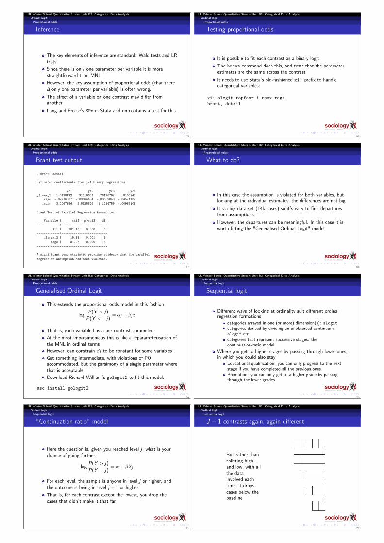
J − 1 contrasts again, again different

But rather thansplitting highand low, with allthe datainvolved eachtime, it dropscases below thebaseline

72







Fitting CR

This model implies one equation for each contrastCan be fitted by hand by defining outcome variable andsubsample for each contrast (ed has 4 values):

gen con1 = ed>1gen con2 = ed>2replace con2 = . if ed<=1gen con3 = ed>3replace con3 = . if ed<=2logit con1 odoby i.osexlogit con2 odoby i.osexlogit con3 odoby i.osex

73







seqlogit

Maarten Buis’s seqlogit does it more or less automatically:

seqlogit ed odoby i.osex, tree(1 : 2 3 4 , 2 : 3 4 , 3 : 4 )

you need to specify the contrastsYou can impose constraints to make parameters equal acrosscontrasts

74






UL Winter School Quantitative Stream Unit B2: Categorical Data AnalysisSpecial topics: depending on interest

Outline





5 Ordinal logit


75






UL Winter School Quantitative Stream Unit B2: Categorical Data AnalysisSpecial topics: depending on interestAlternative specific options

Clogit and the basic idea

If we have information on the outcomes (e.g., how expensivethey are) but not on the individuals, we can use clogit

76






UL Winter School Quantitative Stream Unit B2: Categorical Data AnalysisSpecial topics: depending on interestAlternative specific options

asclogit and practical examples

If we have information on the outcomes and also on theindividuals, we can use asclogit, alternative-specific logitSee examples in Long and Freese

77






UL Winter School Quantitative Stream Unit B2: Categorical Data AnalysisSpecial topics: depending on interestModels for count data

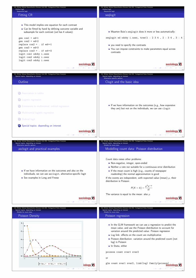
Modelling count data: Poisson distribution

Count data raises other problems:Non-negative, integer, open-endedNeither a rate nor suitable for a continuous error distributionIf the mean count is high (e.g., counts of newspaperreadership) the normal approximation is good

If the events are independent, with expected value (mean) µ, theirdistribution is Poisson:

P(X = k) =µke−µ

k!

The variance is equal to the mean: also µ

78







Poisson Density

79







Poisson regression

In the GLM framework we can use a regression to predict themean value, and use the Poisson distribution to account forvariation around the predicted value: Poisson regressionLog link: effects on the count are multiplicativePoisson distribution: variation around the predicted count (notlog) is PoissonIn Stata, either

poisson count xvar1 xvar2

or

glm count xvar1 xvar2, link(log) family(poisson)

80







Over dispersion

If the variance is higher than predicted, the SEs are not correctThis may be due to omitted variablesOr to events which are not independent of each otherAdding relevant variables can help

81







Negative binomial regression

Negative binomial regression is a form of poisson regressionthat takes an extra parameter to account for overdispersion. Ifthere is no overdispersion, poisson is more efficient

82







Zero inflated, zero-truncated

Another issue with count data is the special role of zeroSometimes we have zero-inflated data, where there is a subsetof the population which is always zero and a subset whichvaries (and may be zero). This means that there are morezeros than poisson would predict, which will bias its estimates.Zero-inflated poisson (zip) can take account of this, bymodelling the process that leads to the all-zeroes stateZero-inflated negative binomial (zinb) is a version that alsocopes with over dispersionZero truncation also arises, for example in data collectionschemes that only see cases with at least one event. ztp dealswith this.

83

Documents

UL Winter School Quantitative Stream Unit B2: …teaching.sociology.ul.ie/ws/wsCatDatsl8.pdfUL Winter School Quantitative Stream Unit B2: Categorical Data Analysis ... 6 UL Winter