UDC 004.94:621.51 doi: 10.32620/aktt.2021.5.03 J. JACOBY

ISSN 1727-7337 (print)

АВІАЦІЙНО-КОСМІЧНА ТЕХНІКА І ТЕХНОЛОГІЯ, 2021, № 5(175) ISSN 2663-2217 (online) 24

UDC 004.94:621.51 doi: 10.32620/aktt.2021.5.03

J. JACOBY, T. BAILEY, V. ZHARIKOV

Tri-Sen Turbomachinery Controls Systems, Houston Texas, USA

CONSIDERATIONS AND COMPLICATIONS WITH "FIRST PRINCIPLES"

DYNAMIC MODELLING OF INDUSTRIAL COMPRESSORS

Readily available processing hardware and "off-the-shelf" (OTS) simulation software has made "high fidelity"

first principles models of both steady and transient states, for both axial and centrifugal industrial compressors,

relatively easy to construct. These high-fidelity models are finding their way into "real-time. digital twin" per-

formance monitors, front-end engineering design, and post-design – pre-construction compressor performance

evaluation. The compressor models are useful for reliably demonstrating the compressor and – to some degree,

based on the complexity of the model – process response to various operating conditions. Once the model is

constructed, it is trivial to run a "what-if" analysis of compressor performance to answer questions related to

(a) recommendations or validation of the recycle/vent valve size and actuation speed, (b) general piping layout

and sizing around the compressor, (c) and hot gas bypass requirements, to name a few. This paper takes a

practical approach in discussing the compressor and process parameters necessary for building these dynamic

"high-fidelity" industrial-compressor models. We identify compressor inputs and compressor responses that are

faithfully modeled by first-principle equations available in the simulation software and those that typically re-

quire a compromise between an "ab initio" and data-fitting approximation. We discuss the simulation's tendency

to overstate pressure excursions during surge events and understate the compressor operation in the "stonewall"

region. We also discuss using the simulator software's compressor-stage enthalpy calculations to predict and

quantify the compressor train reverse rotation. We use our broad experience and understanding of the compres-

sor operation and simulation and our experience with the AVEVA™ Dynamic-Simulation "OTS" simulation

software as the basis for this discussion.

Keywords: compressor model; high fidelity; first principles; industrial compressors; dynamic simulation; com-

pressor surge; compressor stonewall; choke flow; steady state; transient; surge event; recycle; vent; reverse

rotation.

Introduction

Industrial compressors are used throughout energy

processing and are an integral part of midstream (pipe-

line) and downstream (refining, LNG, chemicals) and

storage processes. These processes include transporta-

tion, refrigeration, separation, and generation of reaction

pressure.

The purpose of this paper is to promote further dis-

cussion concerning foundational considerations, limita-

tions, and “workarounds” in the modelling of industrial

compressor transient operation using off-the-shelf (com-

mercially available), high-fidelity, process simulation

software.

Definitions

First-Principles (ab initio) modelling.

First-principles models, in general, are built using

established laws of chemistry and physics without

additional assumptions, inference, or modifications

based upon empirical testing or data fitting. This paper

discusses using the first principles equations of state

included in the Dynamic Simulation high fidelity

modelling software [1] and the assumptions and

inference associated with the compressor data inputs

required to make the models work.

High Fidelity modelling.

As far as we are aware, there are no absolute criteria

for what constitutes “high-fidelity” for industrial

compressor modeling. Like most things, there is a

diminishing marginal utility for model tuning, and we

“overlay” an engineering sensibility to compressor

modelling where; “close enough is good enough.” We

define a compressor model as high-fidelity if it generates

temperatures, pressures, and flows that match the

compressor manufacturers API617 data sheets or the

end-users heat and material balance at a steady-state,

within 1.0%.

Dynamic Compressor Modelling.

Dynamic compressor models are typically designed

to assess compressor operation and performance both

from the standpoint of compressor protection (surge and

J. Jacoby, T. Bailey, V. Zharikov, 2021

Двигуни і енергоустановки літальних апаратів

25

stonewall), and from a process operations perspective.

Compressor models are used to evaluate compressor re-

cycle/vent valve sizing, the recycle/vent valve associated

actuator speed of response, compressor piping size and

volume, and the design and suitability of the compressor

controls. The discussions in this paper are limited to the

transient compressor operation viewpoint (as opposed to

steady-state, except when constructing the model.) These

transient operations typically include startup, trip, and

process upsets and failures (e.g., unusual, and rapid pro-

cess changes that affect compressor discharge pres-

sure) [2].

Compressor Performance Map.

To evaluate the transient compressor operation, we

start with the compressor manufacturer's performance

curve. The performance curves typically include multiple

speed lines (for variable speed machines or machines

with inlet guide vanes), a single-speed line (for constant

speed machines), the surge points for the speed lines, a

guaranteed point, and efficiency curves. In addition, the

performance curve also specifies the compressor inlet

conditions, inlet feed MW, compressibility, and the spe-

cific heat ratio (K) or the polytropic efficiency (η). A per-

formance “curve” is provided for each compressor stage.

Fig. A. Representation of typical compressor

performance curve [3]

Compressor Surge.

In “Application Guideline for Centrifugal Compres-

sor Surge Control Systems”, the surge is defined as “the

operating point at which the compressor peak head capa-

bility and minimum flow limit are reached” [2]. Com-

pressor operational excursions to the “left” of the surge

line are typically referred to as unstable. These excur-

sions (surge events) are created by abnormally high com-

pressor discharge pressure (head). They can result in

compressor flow reversals (which lower the discharge

pressure), creating a surge cycle. Surge events can cause

severe damage to the compressor, including; bearing fail-

ure, impeller rubbing, and seal damage [4].

Fig. B. Representation of typical compressor

surge “region”

Compressor Stonewall.

Compressor Stonewall or Choke is an operating

condition (low discharge pressure and high flow rate for

a given speed line) where the velocity of the gas for a

given compressor stage has accelerated to Mach-1, and

no further increase in flow is possible [5].

Fig. C. Representation of typical compressor Stonewall

or chocked flow “region”



Compressor manufacturers have found that pro-

longed compressor operation in stonewall can lead to fa-

tigue failures of the impeller cover and blades. There is

also an increase in the compressor discharge temperature

due to the rise in entropy across the region of sonic ve-

locity [5].

Considerations

Compressor model data inputs.

To build a credible “high-fidelity” compressor

model, the following data is required:

Driver (motor or turbine data) including power,

torque, speed gearing;

Compressor performance curves – to model

compressor characteristics (head/capacity relationship);

Manufacturers compressor data sheets

(API617) – to validate the steady-state model;

Process heat and material balance (if available)-

to validate the steady-state model;

Process isometric drawings – to determine pip-

ing volumes and pressure drops;

Process and instrumentation drawings (P&ID) –

to determine compressor, vessel, and piping arrange-

ment;

Process flow diagram (PFD) – important com-

pressor, vessel, and piping arrangement;

Valve data – recycle valves, block valves, con-

trol valves, check valves, etc.- to model CV, and valve

flow characteristics;

Valve Actuator data – to model valve speed of

response;

Heat exchanger data – to model heat exchangers

(capacity, heat transfer characteristics, flow rates, and

temperatures for fluid streams).

Compressor Model Boundaries.

In general, the compressor model starts at the clos-

est significant volume outside of the recycle loop (vessel,

etc.) on the inlet of the compressor. The compressor

model typically ends after the first check valve outside of

the recycle loop on the discharge side of the compressor.

For refrigeration compressor models, it may be necessary

to model the discharge condensers and liquid accumula-

tors.

Equations of State (EOS) Selection.

Modern “off-the-shelf” high fidelity modelling soft-

ware platforms offer a selection of first-principles equa-

tion-of-state simulation selections for use in modelling a

compressor. These selections include [1]:

Industrial Steam Tables;

Braun K10;

Redlich-Kwong (RK) ;

Soave-Redlich-Kwong (SRK) and derivatives;

Peng- Robinson (PR) and derivatives;

Others.

The difficulty associated with multiple “EOSs” is

deciding and choosing which EOS to use for a given

compressor model. When building the compressor

model, we typically start with the SRK EOS, and com-

pare parameters for a given steady-state compressor con-

dition (pressure, temperature, flow), with the compressor

manufacturers' performance data sheets or the process

heat and material balance sheet, or both.

If the model is in close agreement (within 1.0%) of

the performance data or material balance, we use that

EOS to evaluate transient conditions. If the EOS results

in steady-state conditions that differ from the compressor

manufacturers performance data sheets or the process

heat and material balance sheet by more than 1.0%, we

iterate the different available EOSs until we find the

“best” EOS fit.

Modelling Inertia.

For a high-fidelity model, the entire compressor

train inertia needs to be considered. Typically, this data

is available from the compressor manufacturer. If the

data is unavailable, the compressor train inertia can be

inferred from operation data (specifically, coast down

data).

Modelling Friction Losses.

Modelling friction losses improves the fidelity of

the model characteristics for a shutdown. Friction losses

are typically modelled using a small percentage (1…2%)

of power (linear relationship). In general, friction losses

are determined empirically.

Modelling Windage Losses.

OTS simulation packages typically have windage

loss inputs, but most compressor manufacturers include

windage losses in their performance curves.

Complications

Compressor feed-gas composition:

Feed-gas composition for ethylene refrigeration,

propylene refrigeration, chlorine, compression, and air

applications are typically simple, with straightforward

chemistry, and can be used directly with the simulator

package equations of state. On the other hand, there are

feeds, including cracked gas, wet gas, and recycle gas ap-

plications, that can be problematic because of the com-

plicated process flow, feed composition, and chemistry.

For example, the cracked gas feed used in an “Eth-

ylene” production process can include more than 40 com-

ponents (Tabl. 1):


27

Fig. D. Simplified crack gas process flow diagram (level controls, check valves,

flow elements etc. omitted for simplicity)

Table 1

Crack gas feed from 3rd party data analysis

(CMF = component mole flow (as a percentage of flow)

Component CMF

H2O 33.556%

ETHYLENE 22.751%

HYDROGEN 21.080%

METHANE 8.474%

ETHANE 8.094%

PROPYLENE 2.422%

N-BUTANE 1.634%

1,3-BUTADIENE 0.465%

PROPANE 0.280%

ACETYLENE 0.261%

BENZENE 0.219%

1-BUTENE 0.138%

C7+ 0.133%

CYCLOPENTADIENE 0.072%

1,4-PENTADIENE 0.053%

TOLUENE 0.037%

TRANS-2-BUTENE 0.036%

CARBON-MONOXIDE 0.032%

N-PENTANE 0.032%

CIS-2-BUTENE 0.028%

METHYL-ACETYLENE 0.028%

STYRENE 0.028%

O-XYLENE 0.020%

PROPADIENE 0.019%

VINYLACETYLENE 0.017%

NAPHTHALENE 0.013%

1-PENTENE 0.013%

ISOBUTYLENE 0.010%

N-HEXANE 0.008%

1-PHENYLNAPHTHALENE 0.006%

METHYLCYCLOPENTADIENE 0.006%

1-METHYLINDENE 0.005%

Table 1 (continued)

Component CMF

1-METHYL-2-ETHYLBENZENE 0.004%

N-OCTADECYLBENZENE 0.004%

INDENE 0.004%

ALPHA-METHYL-STYRENE 0.003%

ETHYLBENZENE 0.003%

CYCLOHEPTENE 0.003%

ISOBUTANE 0.002%

2-METHYL-1,3-BUTADIENE 0.002%

CARBON-DIOXIDE 0.002%

Etc. (4 components less than .002%) 0.001%

100.00%

Molecular Weight (as given) 19.7

Because of the chemical complexity and variations

of this feed and to reduce simulation processing load (cal-

culating performance), the cracked gas feed composition

is often simplified. This simplification is accomplished

by “lumping” components that are “materially insignifi-

cant” individually (less than 0.5% of feed) but added to-

gether must be accounted for. This creates a quasi-hybrid

model that uses first principles equations of state and data

fitting of the feed.

Table 2

Simplified crack gas feed

Component CMF MW MW by %

H2O 33.69% 18.02 6.07

ETHYLENE 22.84% 28.05 6.41

H2 21.17% 2.02 0.43

METHANE 8.51% 16.04 1.36

ETHANE 8.13% 30.07 2.44



Table 2 (continued) Component CMF MW MW by %

Propylene 2.43% 42.08 1.02

BUTANE 1.64% 58.12 0.95

1,3 Butadiene 0.47% 54.09 0.25

PROPANE 0.28% 44.1 0.12

ACETYLN 0.26% 26.04 0.07

BENZENE 0.22% 78.11 0.17

1BUTENE 0.14% 56.11 0.08

DECANE 0.22% 142.28 0.32

100.00% Calc MW 19.70

This lumping of the minor components in the feed

can have a minor or significant impact on multi-stage

compressor models. As the gas in a multi-stage model

passes through the compressor, heat exchangers, etc., the

different gas components (with similar mole weights)

condense or vaporize at different temperatures and pres-

sure (which the simulation faithfully replicates with the

selected EOS), causing the density of the feed gas to

change as it travels through the compressor model to suc-

cessive stages. If the component “lumping” or simplifi-

cation is done well, the compressor model performance

will match the compressor data sheets or process heat and

material balance. If the simplification is “off”, the model

will not match the compressor data sheets or process heat

and material balance.

Choosing a component(s) for a “good” simplifica-

tion of the minor components in the complex gas fees is

most often iterative. It often requires significant experi-

ence with the process and model “construction.”

Fig. E. Effect of “low” calculated moleweight

operating point

Fig. F. Effect of “high” calculated moleweight

on operatingpoint

Compressor simulation performance to the

“left” of the surge line (point).

When a compressor works through a surge event

(excessive head), the actual flow quickly decreases to-

wards the y-axis without a further increase in the head.

As the compressor flow reverses, the head begins to fall,

allowing the flow to increase again (compressor recov-

ers) [6]. As the flow increases, if whatever created the

excessively high discharge pressure (head) hasn’t re-

solved, the compressor operating point will move back

towards the surge point and create a surge cycle.

When we configure a performance curve into a sim-

ulation tool, the left-most data point in the performance

curve (high head, low flow) is typically interpreted by the

simulator software as the surge point. An issue we face

when using the Dynamic-Simulator is that the simulation

package interpolates the compressor head to the “left” of

the surge point using a linear approximation with a non-

zero slope (gradual increase in head to the left of the

surge point).

Fig. G. An approximation of “actual” head and flowpast

the last performance data point (surge point)

Fig. H. A typical OTS approximation of head past

the last performance data point (surge point)


29

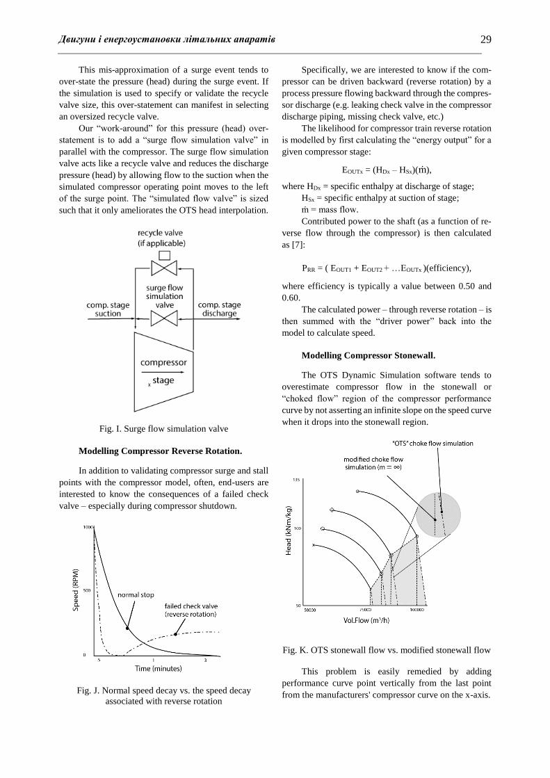
This mis-approximation of a surge event tends to

over-state the pressure (head) during the surge event. If

the simulation is used to specify or validate the recycle

valve size, this over-statement can manifest in selecting

an oversized recycle valve.

Our “work-around” for this pressure (head) over-

statement is to add a “surge flow simulation valve” in

parallel with the compressor. The surge flow simulation

valve acts like a recycle valve and reduces the discharge

pressure (head) by allowing flow to the suction when the

simulated compressor operating point moves to the left

of the surge point. The “simulated flow valve” is sized

such that it only ameliorates the OTS head interpolation.

Fig. I. Surge flow simulation valve

Modelling Compressor Reverse Rotation.

In addition to validating compressor surge and stall

points with the compressor model, often, end-users are

interested to know the consequences of a failed check

valve – especially during compressor shutdown.

Fig. J. Normal speed decay vs. the speed decay

associated with reverse rotation

Specifically, we are interested to know if the com-

pressor can be driven backward (reverse rotation) by a

process pressure flowing backward through the compres-

sor discharge (e.g. leaking check valve in the compressor

discharge piping, missing check valve, etc.)

The likelihood for compressor train reverse rotation

is modelled by first calculating the “energy output” for a

given compressor stage:

EOUTx = (HDx – HSx)(ṁ),

where HDx = specific enthalpy at discharge of stage;

HSx = specific enthalpy at suction of stage;

ṁ = mass flow.

Contributed power to the shaft (as a function of re-

verse flow through the compressor) is then calculated

as [7]:

PRR = ( EOUT1 + EOUT2 + …EOUTx )(efficiency),

where efficiency is typically a value between 0.50 and

0.60.

The calculated power – through reverse rotation – is

then summed with the “driver power” back into the

model to calculate speed.

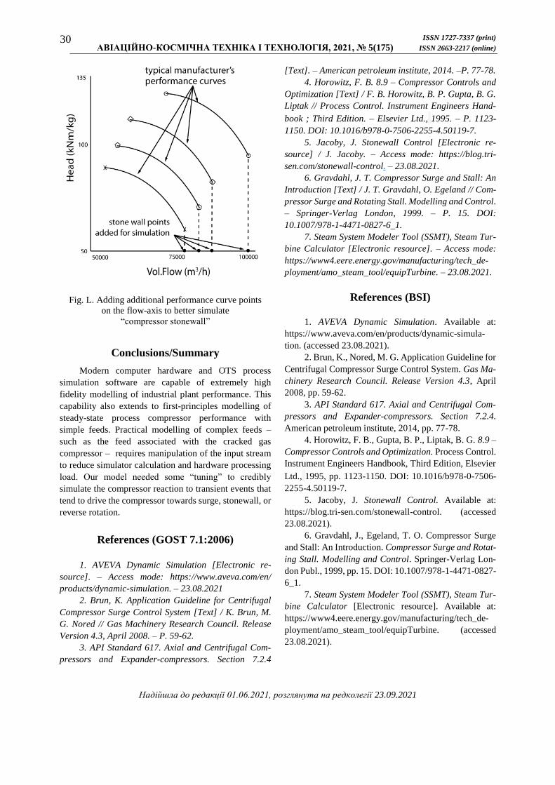
Modelling Compressor Stonewall.

The OTS Dynamic Simulation software tends to

overestimate compressor flow in the stonewall or

“choked flow” region of the compressor performance

curve by not asserting an infinite slope on the speed curve

when it drops into the stonewall region.

Fig. K. OTS stonewall flow vs. modified stonewall flow

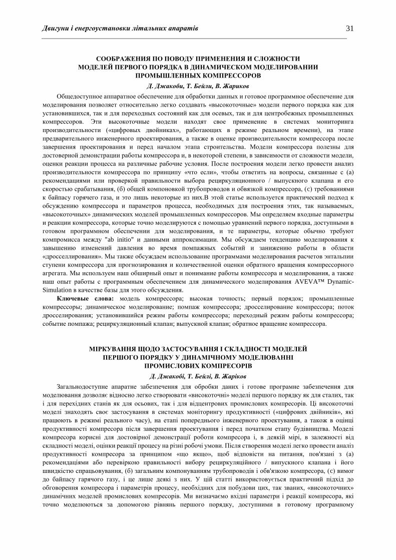
This problem is easily remedied by adding

performance curve point vertically from the last point

from the manufacturers' compressor curve on the x-axis.



Fig. L. Adding additional performance curve points

on the flow-axis to better simulate

“compressor stonewall”

Conclusions/Summary

Modern computer hardware and OTS process

simulation software are capable of extremely high

fidelity modelling of industrial plant performance. This

capability also extends to first-principles modelling of

steady-state process compressor performance with

simple feeds. Practical modelling of complex feeds –

such as the feed associated with the cracked gas

compressor – requires manipulation of the input stream

to reduce simulator calculation and hardware processing

load. Our model needed some “tuning” to credibly

simulate the compressor reaction to transient events that

tend to drive the compressor towards surge, stonewall, or

reverse rotation.

References (GOST 7.1:2006)

1. AVEVA Dynamic Simulation [Electronic re-

source]. – Access mode: https://www.aveva.com/en/

products/dynamic-simulation. – 23.08.2021

2. Brun, K. Application Guideline for Centrifugal

Compressor Surge Control System [Text] / K. Brun, M.

G. Nored // Gas Machinery Research Council. Release

Version 4.3, April 2008. – P. 59-62.

3. API Standard 617. Axial and Centrifugal Com-

pressors and Expander-compressors. Section 7.2.4

[Text]. – American petroleum institute, 2014. –P. 77-78.

4. Horowitz, F. B. 8.9 – Compressor Controls and

Optimization [Text] / F. B. Horowitz, B. P. Gupta, B. G.

Liptak // Process Control. Instrument Engineers Hand-

book ; Third Edition. – Elsevier Ltd., 1995. – P. 1123-

1150. DOI: 10.1016/b978-0-7506-2255-4.50119-7.

5. Jacoby, J. Stonewall Control [Electronic re-

source] / J. Jacoby. – Access mode: https://blog.tri-

sen.com/stonewall-control. – 23.08.2021.

6. Gravdahl, J. T. Compressor Surge and Stall: An

Introduction [Text] / J. T. Gravdahl, O. Egeland // Com-

pressor Surge and Rotating Stall. Modelling and Control.

– Springer-Verlag London, 1999. – P. 15. DOI:

10.1007/978-1-4471-0827-6_1.

7. Steam System Modeler Tool (SSMT), Steam Tur-

bine Calculator [Electronic resource]. – Access mode:

https://www4.eere.energy.gov/manufacturing/tech_de-

ployment/amo_steam_tool/equipTurbine. – 23.08.2021.

References (BSI)

1. AVEVA Dynamic Simulation. Available at:

https://www.aveva.com/en/products/dynamic-simula-

tion. (accessed 23.08.2021).

2. Brun, K., Nored, M. G. Application Guideline for

Centrifugal Compressor Surge Control System. Gas Ma-

chinery Research Council. Release Version 4.3, April

2008, pp. 59-62.

3. API Standard 617. Axial and Centrifugal Com-

pressors and Expander-compressors. Section 7.2.4.

American petroleum institute, 2014, pp. 77-78.

4. Horowitz, F. B., Gupta, B. P., Liptak, B. G. 8.9 –

Compressor Controls and Optimization. Process Control.

Instrument Engineers Handbook, Third Edition, Elsevier

Ltd., 1995, pp. 1123-1150. DOI: 10.1016/b978-0-7506-

2255-4.50119-7.

5. Jacoby, J. Stonewall Control. Available at:

https://blog.tri-sen.com/stonewall-control. (accessed

23.08.2021).

6. Gravdahl, J., Egeland, T. O. Compressor Surge

and Stall: An Introduction. Compressor Surge and Rotat-

ing Stall. Modelling and Control. Springer-Verlag Lon-

don Publ., 1999, pp. 15. DOI: 10.1007/978-1-4471-0827-

6_1.

7. Steam System Modeler Tool (SSMT), Steam Tur-

bine Calculator [Electronic resource]. Available at:

https://www4.eere.energy.gov/manufacturing/tech_de-

ployment/amo_steam_tool/equipTurbine. (accessed

23.08.2021).

Надійшла до редакції 01.06.2021, розглянута на редколегії 23.09.2021


31

СООБРАЖЕНИЯ ПО ПОВОДУ ПРИМЕНЕНИЯ И СЛОЖНОСТИ

МОДЕЛЕЙ ПЕРВОГО ПОРЯДКА В ДИНАМИЧЕСКОМ МОДЕЛИРОВАНИИ

ПРОМЫШЛЕННЫХ КОМПРЕССОРОВ

Д. Джакоби, T. Бейли, В. Жариков

Общедоступное аппаратное обеспечение для обработки данных и готовое программное обеспечение для

моделирования позволяет относительно легко создавать «высокоточные» модели первого порядка как для

установившихся, так и для переходных состояний как для осевых, так и для центробежных промышленных

компрессоров. Эти высокоточные модели находят свое применение в системах мониторинга

производительности («цифровых двойниках», работающих в режиме реальном времени), на этапе

предварительного инженерного проектирования, а также в оценке производительности компрессора после

завершения проектирования и перед началом этапа строительства. Модели компрессора полезны для

достоверной демонстрации работы компрессора и, в некоторой степени, в зависимости от сложности модели,

оценки реакции процесса на различные рабочие условия. После построения модели легко провести анализ

производительности компрессора по принципу «что если», чтобы ответить на вопросы, связанные с (а)

рекомендациями или проверкой правильности выбора рециркуляционного / выпускного клапана и его

скоростью срабатывания, (б) общей компоновкой трубопроводов и обвязкой компрессора, (c) требованиями

к байпасу горячего газа, и это лишь некоторые из них.В этой статье используется практический подход к

обсуждению компрессора и параметров процесса, необходимых для построения этих, так называемых,

«высокоточных» динамических моделей промышленных компрессоров. Мы определяем входные параметры

и реакции компрессора, которые точно моделируются с помощью уравнений первого порядка, доступными в

готовом программном обеспечении для моделирования, и те параметры, которые обычно требуют

компромисса между "ab initio" и данными аппроксимации. Мы обсуждаем тенденцию моделирования к

завышению изменений давления во время помпажных событий и занижению работы в области

«дросселлирования». Мы также обсуждаем использование программами моделирования расчетов энтальпии

ступени компрессора для прогнозирования и количественной оценки обратного вращения компрессорного

агрегата. Мы используем наш обширный опыт и понимание работы компрессора и моделирования, а также

наш опыт работы с программным обеспечением для динамического моделирования AVEVA™ Dynamic-

Simulation в качестве базы для этого обсуждения.

Ключевые слова: модель компрессора; высокая точность; первый порядок; промышленные

компрессоры; динамическое моделирование; помпаж компрессора; дросселирование компрессора; поток

дросселирования; установившийся режим работы компрессора; переходный режим работы компрессора;

событие помпажа; рециркуляционный клапан; выпускной клапан; обратное вращение компрессора.

МІРКУВАННЯ ЩОДО ЗАСТОСУВАННЯ І СКЛАДНОСТІ МОДЕЛЕЙ

ПЕРШОГО ПОРЯДКУ У ДИНАМІЧНОМУ МОДЕЛЮВАННІ

ПРОМИСЛОВИХ КОМПРЕСОРІВ

Д. Джакобі, T. Бейлі, В. Жаріков

Загальнодоступне апаратне забезпечення для обробки даних і готове програмне забезпечення для

моделювання дозволяє відносно легко створювати «високоточні» моделі першого порядку як для сталих, так

і для перехідних станів як для осьових, так і для відцентрових промислових компресорів. Ці високоточні

моделі знаходять своє застосування в системах моніторингу продуктивності («цифрових двійників», які

працюють в режимі реального часу), на етапі попереднього інженерного проектування, а також в оцінці

продуктивності компресора після завершення проектування і перед початком етапу будівництва. Моделі

компресора корисні для достовірної демонстрації роботи компресора і, в деякій мірі, в залежності від

складності моделі, оцінки реакції процесу на різні робочі умови. Після створення моделі легко провести аналіз

продуктивності компресора за принципом «що якщо», щоб відповісти на питання, пов'язані з (а)

рекомендаціями або перевіркою правильності вибору рециркуляційного / випускного клапана і його

швидкістю спрацьовування, (б) загальним компонуванням трубопроводів і обв'язкою компресора, (c) вимог

до байпасу гарячого газу, і це лише деякі з них. У цій статті використовується практичний підхід до

обговорення компресора і параметрів процесу, необхідних для побудови цих, так званих, «високоточних»

динамічних моделей промислових компресорів. Ми визначаємо вхідні параметри і реакції компресора, які

точно моделюються за допомогою рівнянь першого порядку, доступними в готовому програмному



забезпеченні для моделювання, і ті параметри, які зазвичай вимагають компромісу між "ab initio" і даними

апроксимації. Ми обговорюємо тенденцію моделювання до завищення змін тиску під час помпажних подій і

заниження роботи в області «дроселювання». Ми також обговорюємо використання програмами

моделювання розрахунків ентальпії ступені компресора для прогнозування і кількісної оцінки зворотного

обертання компресорного агрегату. Ми використовуємо наш великий досвід і розуміння роботи компресора і

моделювання, а також наш досвід роботи з програмним забезпеченням для динамічного моделювання

AVEVA™ Dynamic-Simulation в якості бази для цього обговорення.

Ключові слова: модель компресора; висока точність; перший порядок; промислові компресори;

динамічне моделювання; помпаж компресора; дроселювання компресора; потік дроселювання; сталий режим

роботи компресора; перехідний режим роботи компресора; подія помпажу; рециркуляційний клапан;

випускний клапан; зворотне обертання компресора.

Джеймс Джакоби – Бакалавр машиностроения, Старший вице-президент в Трай-Сен системы управле-

ния турбомашинным оборудованием, Хьюстон, штат Техас, США.

email: [email protected]

Томас Бейли – Бакалавр экономики, МБА, Директор по маркетингу в Трай-Сен системы управления

турбомашинным оборудованием, Хьюстон, штат Техас, США.

Виталий Жариков – Магистр машиностроения, Инженер проекта в Трай-Сен системы управления тур-

бомашинным оборудованием, Хьюстон, штат Техас, США.

James Jacoby – BS Mechanical Engineering, Senior Vice President at Tri-Sen Turbomachinery Controls

Systems, Houston Texas, USA,

e-mail: [email protected], ORCID: 0000-0002-0151-6602.

Thomas Bailey – BS Economics, MBA, Director of Marketing at Tri-Sen Turbomachinery Controls


e-mail: [email protected], ORCID: 0000-0003-4210-648X.

Vitalii Zharikov – MS Mechanical Engineering, Project Engineer at Tri-Sen Turbomachinery Controls


e-mail: [email protected], ORCID: 0000-0003-0356-4154.

mailto:[email protected]




Documents

UDC 004.94:621.51 doi: 10.32620/aktt.2021.5.03 J. JACOBY