Embed Size (px)
Citation preview

DISTORTIONAL BUCKLING OF
C AND Z MEMBERS IN BENDING
Progress Report Submitted to: The American Iron and Steel Institute (AISI)
August 2004
Cheng Yu, Ben Schafer
Department of Civil Engineering The Johns Hopkins University
Baltimore, Maryland
i
Table of Contents Abstract ............................................................................................................................... 1 1. Distortional Buckling Test on Cold-Formed Steel Beams ............................................. 2
1.1 Introduction............................................................................................................... 2 1.2 Distortional Buckling Tests ...................................................................................... 3
1.2.1 Selection of Specimen........................................................................................ 3 1.2.2 Testing Setup ..................................................................................................... 6 1.2.3 Panel-to-Purlin Fastener Configuration ............................................................. 7
1.3 Tension Tests ............................................................................................................ 9 1.4 Test Results............................................................................................................. 11 1.5 Examination of Several Tests of Note .................................................................... 14
1.5.1 Test Failed in Lateral-Torsional Buckling Mode: Re-Test of D8C097........... 14 1.5.3 Test Failed by Material Yielding: Test of D3.62C054-3E4W......................... 16 1.5.4 Tests Failed in Local Buckling Mode.............................................................. 17 1.5.2 Tests Failed in Unexpected Mode.................................................................... 18
1.6 Comparison with Local Buckling Tests.................................................................. 19 1.7 Comparison with Current Design Specifications.................................................... 30
2. Finite Element Modeling .............................................................................................. 32 2.1 Introduction............................................................................................................. 32 2.2 Modeling Details and Boundary/Loading Conditions ............................................ 32 2.3 Geometric Imperfection .......................................................................................... 35 2.4 Residual Stress ........................................................................................................ 36 2.5 Comparison with Experimental Results.................................................................. 36 2.6 Extended Finite Element Analysis.......................................................................... 42
3. Stress Gradient Effect on the Buckling of Thin Plates ................................................. 45 3.1 Introduction............................................................................................................. 45 3.2 Analytic Solution: Energy Method ......................................................................... 48 3.3 Stress Gradient on Stiffened Elements ................................................................... 49 3.4 Stress Gradient on Unstiffened Elements ............................................................... 52
3.4.1 Deflection Function and Boundary Conditions ............................................... 53 3.4.2 Deflection Function 1 ...................................................................................... 54 3.4.3 Deflection Function 2 ...................................................................................... 55 3.4.4 Deflection Function 3 ...................................................................................... 56 3.4.5 Verification of Three Deflection Functions..................................................... 57 3.4.6 Results.............................................................................................................. 62
3.5 Discussion ............................................................................................................... 64 4. Conclusions................................................................................................................... 65 Acknowledgement ............................................................................................................ 66 References......................................................................................................................... 66 Appendix: Summary of Recent Work.............................................................. 68
A1. Distortional Buckling Tests ................................................................................... 68 A2. Finite Element Modeling ....................................................................................... 68 A3. Stress Gradient Effect on the Thin Plate................................................................ 69
A3.1 Elastic Buckling ............................................................................................... 69 A3.2 Ultimate Strength ............................................................................................. 71
A4. Partial Restraint Effect on the Distortional Buckling of Cold-Formed Beams...... 73
ii
A5. The Outline of the Doctoral Thesis........................................................................ 74 A6. Reference ............................................................................................................... 77
1
Abstract
Laterally braced cold-formed steel beams generally fail due to local and/or distortional buckling in combination with yielding. For many cold-formed steel studs, joists, purlins, or girts, distortional buckling may be the predominant buckling mode, unless the compression flange is partially restrained by attachment to sheathing or paneling. Distortional buckling of cold-formed steel C and Z members in bending remains a largely unaddressed problem in the current North American Specification for the Design of Col-Formed Steel Structural Members (NAS 2001). Further, adequate experimental data on unrestricted distortional buckling in bending is unavailable. Therefore, a series of distortional buckling tests on C and Z members in bending has been completed at the structural testing lab of Johns Hopkins University. These tests are essentially the extended research (phase 2) of a recently completed experimental project on local buckling of C and Z beams (phase 1, as summarized in Yu and Schafer 2003). This second phase of four point bending tests use nominally identical specimens to the first phase and a similar testing setup. However, the corrugated panel attached to the compression flange is removed in the constant moment region so that distortional buckling may occur. The experimental data is being used to help develop and validate an efficient and reliable design procedure for C and Z members in bending.
A nonlinear inelastic finite element model by ABAQUS was setup and verified by the experiment results. The FE model considers the geometric imperfection and the material nonlinearity. The finite element analysis is extended to a broader range of section dimensions, material properties, restraint, and loading conditions.
This report also presents an analytical method to calculate the elastic buckling stress of the rectangular thin plate under nonuniform applied axial stresses. Two cases are considered, buckling of a plate simply supported on all four sides and buckling of a plate simply supported on three sides with one unloaded edge free and the opposite unloaded edge rotationally restrained. These two cases illustrate the influence of stress (moment) gradient on stiffened and unstiffened elements, respectively. The axial stress gradient is equilibrated by shear forces along the supported edges. A Rayleigh-Ritz solution with an assumed deflection function as a combination of a polynomial and trigonometric series is employed. Finite element analysis using ABAQUS validates the analytical model derived herein. The results help establish a better understanding of the stress gradient effect on typical thin plates and are intended to lead to the development of design provisions to account for the influence of moment gradient on local and distortional buckling of thin-walled beams.

2
1. Distortional Buckling Test on Cold-Formed Steel Beams
1.1 Introduction
Determination of the ultimate bending capacity of cold-formed steel C and Z members is complicated by yielding and the potential for local, distortional, and lateral-torsional buckling of the section, as shown in the finite strip analysis of Figure 1.
102
103
104
0
0.5
1
1.5
half−wavelength (mm)
Mcr
/ M
y
AISI96 Ex. 1−10
My=12.75kN−m
Local Mcr
/My=0.86 Dist. M
cr/M
y=0.65
Lateral−torsional
Figure 1 Buckling modes of a cold-formed steel beam
Existing experimental and analytical work indicates that the current North American Specification provisions (NAS 2001) are inadequate for predicting bending capacity of C and Z members when distortional buckling occurs (e.g., Hancock et al. 1996, Rogers and Schuster 1995, Schafer and Peköz 1999, Yu and Schafer 2002).
To investigate this problem, a joint MBMA-AISI project was recently completed at Johns Hopkins University entitled: Test Verification of Effect of Stress Gradient on Webs of Cee and Zee Sections. This “Phase 1” testing focused on the role of web slenderness in local buckling failures. A panel was through-fastened to the compression flange at a close fastener spacing to insure that distortional buckling and lateral-torsional buckling were restricted. The “Phase 1” testing provided the upper-bound capacity for a bending member failing in the local mode. This progress report details “Phase 2” work on distortional buckling of the same C and Z members examined in Phase 1. Although many C and Z members in bending have attachments (panel or otherwise), which stabilize the compression flange and help restrict distortional buckling, many do not. Negative bending of continuous members (joists, purlins, etc.) and wind suction on walls and panels (without interior sheathing) are common examples where no such beneficial attachments exist – these members are prone to distortional failures. Even when attachment to the compression flange exists it may not fully restrict distortional buckling, as may be the case for thin panels with large center-to-center fastener spacing and/or thick insulation between the purlin and panel. Flexural members are typically more prone
3
to distortional failures than compression members, due to the dominance of local web buckling in standard compression members. Geometry, unique to flexural members, such as the sloping lip stiffener used in Zs is inefficient in retarding distortional buckling. For example, a typical 8 in. deep Z with t = 0.120 in. has a distortional buckling stress that is ½ the local buckling stress. The advent of higher strength steels also increases the potential for distortional failures (Schafer and Peköz 1999, Schafer 2002a). In many flexural members, left unrestricted, distortional buckling is the expected failure mode.
1.2 Distortional Buckling Tests
1.2.1 Selection of Specimen
The distortional buckling tests reported here employ nominally the same geometry as the previously conducted local buckling tests. Specimens were selected to provide systematic variation in web slenderness (h/t) while also varying the other non-dimensional parameters that govern the problem such as flange slenderness (b/t), edge stiffener slenderness (d/t) and relevant interactions, such as the web height to flange width (h/b) ratio. However, as commercially available sections were used, the manner in which the h/t variation could be completed was restricted by the availability of sections. A selection of the cross-sections selected for testing is summarized in Figure 2 and Table 1.
Table 1 Summary of specimens selected for testing
h/t b/t d/t h/b d/b Performed Tests number min max min max min max min max min max Group 1 Z: h, b ~d fixed, t varied 7 71.3 138.2 21.9 39.3 7.0 13.4 3.2 3.6 0.28 0.37 Group 2 Z: h, b ~d fixed, t varied 2 126.6 140.4 38.6 42.0 10.1 11.5 3.2 3.3 0.26 0.28 Group 3 C: h, b d fixed, t varied 8 80.7 241.7 20.3 59.1 6.4 20.3 3.8 4.1 0.26 0.35 Group 4 C: b, d fixed, h, t varied 7 66.9 186.7 30.9 43.1 6.4 12.9 2.0 6.0 0.19 0.31
Total 24 66.9 241.7 20.3 59.1 6.4 20.3 2.0 6.0 0.19 0.37
Figure 2 Typical geometry of tested C and Z members
Geometry of the C and Z members used in the distortional buckling tests is summarized in Figure 3. The dimensions of the specimens were recorded at mid-length and mid-distance between the center and loading points, for a total of three measurement locations for each specimen. The mean dimensions, as determined from the three sets of measurements, are given in Table 2.

4
t t
h h
rht
rdt rht
rdt
bt bt
θt
bc bc
dt dt
rhc rdc θc
rhc rdc
dc
θt
dc
θc
Figure 3 Definitions of specimen dimensions for Z and C
The variables used for the dimensions and the metal properties are defined as follows:
h out-to-out web depth
bc out-to-out compression flange width
dc out-to-out compression flange lip stiffener length
θc compression flange stiffener angle from horizontal
bt out-to-out tension flange width
dt out-to-out compression flange lip stiffener length
θt tension flange stiffener angle from horizontal
rhc outer radius between web and compression flange
rdc outer radius between compression flange and lip
rht outer radius between web and tension flange
rdt outer radius between tension flange and lip
t base metal thickness
fy yield stress
E modulus of elasticity
5
Table 2 Measured geometry of beams for distortional buckling tests
Group No. Test label Specimen h
(in.) bc
(in.) dc
(in.) θc
(deg) bt
(in.) dt
(in.) θt
(deg) rhc
(in.) rdc (in.)
rht (in.)
rdt (in.)
t (in.)
fy (ksi)
D8.5Z120-4E1W D8.5Z120-4 8.44 2.63 0.93 54.20 2.47 1.00 50.20 0.34 0.34 0.34 0.34 0.1181 61.35 D8.5Z120-1 8.43 2.65 0.94 48.10 2.52 0.99 52.10 0.36 0.36 0.35 0.35 0.1181 61.89
D8.5Z115-1E2W D8.5Z115-2 8.54 2.56 0.91 49.00 2.40 0.89 48.30 0.35 0.35 0.37 0.37 0.1171 64.14 D8.5Z115-1 8.50 2.66 0.82 48.33 2.47 0.87 48.30 0.37 0.37 0.39 0.39 0.1166 65.79
D8.5Z092-3E1W D8.5Z092-3 8.40 2.58 0.95 51.90 2.41 0.94 51.60 0.29 0.29 0.31 0.31 0.0893 57.59 D8.5Z092-1 8.42 2.59 0.93 52.40 2.39 0.95 50.90 0.28 0.28 0.31 0.31 0.0897 57.75
D8.5Z082-4E3W D8.5Z082-4 8.48 2.52 0.94 48.50 2.39 0.97 51.30 0.28 0.28 0.30 0.30 0.0810 59.21 D8.5Z082-3 8.50 2.53 0.94 49.90 2.37 0.96 49.50 0.28 0.28 0.30 0.30 0.0810 58.99
D8.5Z065-7E6W D8.5Z065-7 8.48 2.47 0.83 50.00 2.47 0.82 49.33 0.32 0.32 0.33 0.33 0.0642 62.36 D8.5Z065-6 8.52 2.48 0.87 53.00 2.43 0.83 48.33 0.32 0.32 0.34 0.34 0.0645 63.34
D8.5Z065-4E5W D8.5Z065-5 8.50 2.36 0.67 51.33 2.52 0.90 47.17 0.27 0.27 0.28 0.28 0.0645 62.79 D8.5Z065-4 8.40 2.40 0.81 47.33 2.25 0.65 51.17 0.30 0.30 0.27 0.27 0.0619 58.26
D8.5Z059-6E5W D8.5Z059-6 8.44 2.42 0.77 50.40 2.39 0.86 48.00 0.32 0.32 0.30 0.30 0.0618 58.54
1
D8.5Z059-5 8.50 2.42 0.80 48.30 2.40 0.76 48.33 0.30 0.30 0.32 0.32 0.0615 59.05 D11.5Z092-3E4W D11.5Z092-4 11.23 3.47 0.94 48.70 3.40 0.91 49.60 0.33 0.33 0.31 0.31 0.0827 69.89
D11.5Z092-3 11.25 3.43 0.89 49.29 3.46 0.87 49.50 0.33 0.33 0.32 0.32 0.0889 70.11 D11.5Z082-3E4W D11.5Z082-4 11.40 3.41 0.88 48.40 3.40 0.86 49.90 0.30 0.30 0.32 0.32 0.0812 73.65
2
D11.5Z082-3 11.33 3.41 0.94 50.20 3.42 0.93 50.97 0.31 0.31 0.31 0.31 0.0818 71.80 D8C097-7E6W D8C097-7 8.13 2.15 0.65 80.75 2.13 0.62 80.00 0.27 0.29 0.27 0.30 0.1001 85.18
D8C097-6 8.15 2.09 0.64 81.00 2.09 0.61 80.00 0.27 0.29 0.27 0.30 0.1005 85.27 D8C097-5E4W D8C097-5 8.06 2.00 0.66 86.70 1.99 0.67 83.00 0.28 0.30 0.28 0.28 0.0998 83.73
D8C097-4 8.06 2.03 0.67 83.00 2.00 0.68 83.00 0.27 0.28 0.27 0.28 0.0998 84.16 D8C085-2E1W D8C085-2 8.06 1.98 0.63 86.00 1.96 0.68 86.60 0.22 0.22 0.23 0.22 0.0825 52.80
D8C085-1 8.06 1.98 0.62 88.60 1.96 0.68 89.00 0.22 0.19 0.23 0.19 0.0848 51.85 D8C068-6E7W D8C068-6 7.94 1.91 0.66 80.00 1.97 0.64 77.80 0.16 0.16 0.16 0.16 0.0708 78.94
D8C068-7 7.94 1.97 0.64 76.50 1.95 0.67 77.50 0.16 0.16 0.16 0.16 0.0708 79.87 D8C054-7E6W D8C054-7 8.01 2.04 0.53 83.40 2.03 0.57 88.70 0.24 0.23 0.21 0.23 0.0528 40.81
D8C054-6 8.00 2.05 0.59 89.40 2.04 0.56 83.30 0.22 0.23 0.23 0.24 0.0520 40.68 D8C045-1E2W D8C045-1 8.18 1.95 0.67 89.00 1.92 0.66 87.60 0.28 0.19 0.22 0.20 0.0348 21.38
D8C045-2 8.14 1.94 0.69 88.80 1.92 0.69 88.30 0.28 0.20 0.23 0.20 0.0348 21.04 D8C043-4E2W D8C043-4 8.02 2.01 0.53 87.30 2.01 0.53 88.80 0.17 0.18 0.17 0.20 0.0459 45.44
D8C043-2 8.03 1.99 0.52 88.93 1.98 0.54 87.70 0.18 0.19 0.20 0.19 0.0472 45.47 D8C033-1E2W D8C033-2 8.15 1.99 0.68 87.10 1.91 0.63 85.80 0.17 0.30 0.20 0.30 0.0337 20.47
3
D8C033-1 8.08 2.00 0.61 86.00 1.96 0.77 88.00 0.21 0.26 0.18 0.28 0.0339 20.35 D12C068-10E11W D12C068-11 12.03 2.03 0.51 81.97 2.00 0.53 85.33 0.22 0.22 0.24 0.23 0.0645 32.90
D12C068-10 12.05 2.02 0.54 85.87 1.98 0.51 94.80 0.24 0.24 0.27 0.23 0.0648 34.70 D12C068-1E2W D12C068-2 11.92 2.05 0.52 82.47 2.03 0.59 77.37 0.26 0.24 0.25 0.24 0.0664 56.31
D12C068-1 11.97 2.12 0.52 80.60 2.00 0.56 83.30 0.25 0.25 0.26 0.26 0.0668 55.86 D10C068-4E3W D10C068-4 10.08 2.00 0.48 83.23 2.08 0.53 83.30 0.26 0.21 0.23 0.23 0.0626 22.01
D10C068-3 10.10 2.07 0.53 80.70 2.08 0.52 81.85 0.24 0.23 0.23 0.22 0.0634 22.54 D10C056-3E4W D10C056-3 9.99 1.97 0.66 88.00 1.95 0.63 89.00 0.13 0.16 0.13 0.13 0.0569 77.28
D10C056-4 10.00 1.94 0.72 88.60 1.92 0.66 87.70 0.13 0.16 0.13 0.18 0.0569 76.93 D10C048-1E2W D10C048-1 9.94 2.06 0.62 86.10 1.94 0.63 79.60 0.20 0.19 0.20 0.19 0.0478 51.08
D10C048-2 9.94 2.02 0.63 85.70 1.95 0.63 83.70 0.18 0.19 0.19 0.20 0.0486 50.62 D6C063-2E1W D6C063-2 5.99 1.99 0.63 88.74 1.97 0.63 87.30 0.19 0.17 0.19 0.22 0.0578 55.94
D6C063-1 5.99 1.99 0.62 87.03 1.97 0.63 86.13 0.22 0.17 0.22 0.17 0.0559 57.82 D3.62C054-3E4W D3.62C054-4 3.73 1.88 0.41 87.00 1.87 0.43 89.00 0.26 0.24 0.27 0.27 0.0555 32.11
4
D3.62C054-3 3.72 1.89 0.35 88.00 1.86 0.36 88.00 0.24 0.28 0.26 0.26 0.0556 32.91
Note: Typical specimen label is DxZ(or C)xxx-x. For example, D8.5Z120-1 means the specimen is 8.5 in. high for the web, Z- section, nominal 0.12 in thick and the beam number is 1. Typical test label is DxZ(or C)xxx-xExW. For example, test D8.5Z120-4E1W means the two-paired specimens are D8.5Z120-4 at the east side and D8.5Z120-1 at the west side.

6
1.2.2 Testing Setup
The basic testing setup is illustrated in Figure 4 through Figure 6. The 16 ft span length, four-point bending test, consists of a pair of 18 ft long C or Z beams in parallel loaded at the 1/3 points. The members are oriented in an opposed fashion, such that in-plane rotation of the C or Z leads to tension in the panel, and thus provides additional restriction against lateral-torsional buckling. Small angles, 1.25 × 1.25 × 0.057 in., are attached to the tension flanges every 12 in. Hot-rolled tube sections, 10 × 7.5 × 6 × 0.25 in., bolt the pair of C or Z beams together at the load points and the supports, and insure shear and web crippling problems are avoided at these locations.
Figure 4 Elevation view of distortional buckling tests
Figure 5 Panel setup for distortional buckling tests
Figure 6 Loading point configuration
7
No panel is placed inside the constant moment region (Figure 5). Instead, the through-fastened panel, t = 0.019 in., 1.25 in. high rib, is attached to the compression flanges in the shear spans only to restrict both the distortional and the lateral-torsional buckling in these regions, but leaving distortional buckling free to form.
The loading system employs a 20 kip MTS actuator, which has a maximum 6 in. stroke. The test was performed in displacement control at a rate of 0.0015 in./sec An MTS 407 controller and load cell monitored the force and insured the desired displacement control was met. Meanwhile, specimen deflections were measured at the 1/3 points with position transducers.
1.2.3 Panel-to-Purlin Fastener Configuration
The panel-to-purlin fastener configuration employed in the distortional buckling tests is the same as that used in the earlier local buckling tests, except the through-fastened panel in the constant moment region is removed. This setup is expected to restrict later-torsional buckling while allowing distortional and local buckling to occur. Examination of the ratio of the elastic distortional buckling moment (McrD) to elastic local buckling moment (McrL) indicates that a large number of members, particularly the Zs, are anticipated to fail in a mechanism dominated by distortional buckling (i.e., McrD/McrL≤1). Even when McrD/McrL>1 distortional buckling may govern because of reduced post-buckling strength in distortional failures (Schafer and Peköz 1999). Table 3 shows the elastic buckling loads of all performed tests. In Table 3, McrL-ABAQUS, McrD-ABAQUS and McrLTB-ABAQUS respectively is elastic local, distortional and lateral-torsional buckling loads calculated by ABAQUS considering the complete testing setup. My is the summation of yield moments of both specimens in each test.
As shown in Table 3, all tests except D8C097-5E4W have either local (McrL-ABAQUS) or distortional buckling (McrD-ABAQUS) to be the first buckling mode and later-torsional buckling (McrLTB-ABAQUS) is successfully restricted. Further, the test setup does not change the local and distortional buckling moments significantly (compare CUFSM results in Table vs. ABAQUS results to observe this). Distortional buckling is expected to be the failure mechanism for all Z beams and local or distortional for the C beams. Figure 7, 8 and 9 show typical elastic buckling results by ABAQUS.

8
Table 3 Elastic buckling loads of performed tests
Test label McrL-
ABAQUS (kips-in.)
McrD-ABAQUS (kips-in.)
McrLTB-ABAQUS (kips-in.)
D8.5Z120-4E1W 1520.6 771.8 1218.8 D8.5Z115-1E2W >1450.7 719.6 1173.7 D8.5Z092-3E1W 684.2 449.6 747.0 D8.5Z082-4E3W 501.0 352.3 >565.6 D8.5Z065-7E6W 253.1 210.7 >301.8 D8.5Z065-4E5W 206.2 173.5 >230.1 D8.5Z059-6E5W 217.7 183.2 >254.9 D11.5Z092-3E4W 633.7 463.8 >760.3 D11.5Z082-3E4W 500.1 385.0 >608.1 D8C097-5E4W 795.7 609.8 533.7 D8C085-2E1W 450.5 396.5 >468.2 D8C068-6E7W 293.9 279.7 >338.1 D8C054-7E6W 116.8 129.2 >144.3 D8C045-1E2W 36.3 >42.5 >42.5 D8C043-4E2W 85.9 >107.1 >107.1 D8C033-1E2W 32.7 >41.6 >41.6 D12C068-1E2W 201.8 208.0 >255.8 D12C068-10E11W 183.2 189.4 >231.9 D10C068-4E3W 184.1 185.9 >226.6 D10C056-3E4W 139.8 >165.5 >165.5 D10C048-1E2W 88.5 >88.5 >88.5 D6C063-2E1W 180.6 162.9 >190.3 D3.62C054-3E4W >120.4 66.4 93.8
Note: lower bounds are given to those modes which are not included in the first 30 eigenmodes calculated in the ABAQUS analysis.
Figure 7 Lateral-torsional buckling mode of beam D8C097-5E4W
9
Figure 8 Distortional buckling mode of beam D8C097-5E4W
Figure 9 Local buckling mode of beam D8C097-5E4W
1.3 Tension Tests
Tension tests were carried out following “ASTM E8–00 Standard Test Methods for Tension Testing of Metallic Material” (ASTM, 2000). Three tensile coupons were taken from the end of each specimen: one from the web flat, one from the compression flange flat, and one from the tension flange flat. A screw-driven ATS 900; with a maximum capacity of 10 kips was used for the loading. An MTS 634.11E-54 extensometer was employed to monitor the deformation. Two methods for yield strength determination were employed: 1) 0.2% Offset Method for the continuous yielding materials; and 2) Auto Graphic Diagram Method for the materials exhibiting discontinuous yielding, Test results are summarized in Table 4. All the Z beams have similar material properties; the yield stresses are between 60 to 70 ksi and for most Z beams the fu/fy ratios are around 130%. On the contrary, the C beams have greatly varying material properties, the yield stresses are measured from 20 to 85 ksi, and the range of fu/fy ratios is from the lowest 101% (for a high strength material) to the highest 207% (for a low strength material). In all cases the tested yield stresses are employed to calculate the beam strength. The elastic moduli E is assumed to be 29500 ksi in all of the members. This E value is supported by tension test results during Phase 1 experiments.

10
Table 4 Summary of tension test results
Specimens t (in.) fy (ksi) fu (ksi) fu / fy D10C068-3 0.0634 22.54 40.87 181% D10C068-4 0.0626 22.01 40.26 183% D11.5Z082-4 0.0812 73.65 93.21 127% D11.5Z082-5 0.0818 71.80 92.02 128% D11.5Z092-2 0.0889 70.11 90.25 129% D11.5Z092-3 0.0827 69.89 89.91 129% D12C068-1 0.0668 55.86 73.61 132% D12C068-10 0.0648 34.70 56.75 164% D12C068-11 0.0645 32.90 56.92 173% D12C068-2 0.0664 56.31 73.69 131% D3.62C054-3 0.0556 32.91 53.32 162% D3.62C054-4 0.0555 32.11 53.56 167% D8.5Z059-1 0.0615 59.05 79.41 134% D8.5Z059-2 0.0618 58.54 79.11 135% D8.5Z065-1 0.0619 58.26 78.44 135% D8.5Z065-2 0.0645 62.79 83.24 133% D8.5Z065-3 0.0645 63.34 83.36 132% D8.5Z065-4 0.0642 62.36 83.47 134% D8.5Z082-3 0.0810 58.99 73.85 125% D8.5Z082-3 0.0810 58.99 73.85 125% D8.5Z082-4 0.0810 59.21 74.02 125% D8.5Z092-1 0.0897 57.75 72.59 126% D8.5Z092-3 0.0893 57.59 72.14 125% D8.5Z115-1 0.1166 65.79 84.67 129% D8.5Z115-2 0.1171 64.14 83.88 131% D8.5Z120-1 0.1181 61.89 83.26 135% D8.5Z120-4 0.1181 61.35 83.10 135% D8C033-1 0.0339 20.35 42.19 207% D8C033-2 0.0337 20.47 41.95 205% D8C043-2 0.0472 45.47 61.01 134% D8C043-4 0.0459 45.44 61.04 134% D8C054-6 0.0520 40.68 50.85 125% D8C054-7 0.0528 40.81 52.52 129% D8C097-5 0.0998 83.73 90.74 108% D8C097-4 0.0998 84.16 91.08 108% D8C068-6 0.0708 78.94 80.75 102% D8C068-7 0.0708 79.87 80.87 101% D8C097-6 0.1005 85.27 91.82 108% D8C097-7 0.1001 85.18 90.77 107% D10C048-1 0.0478 51.08 58.54 115% D10C048-2 0.0486 50.62 57.77 114% D10C056-3 0.0569 77.28 80.38 104% D10C056-4 0.0569 76.93 81.60 106% D8C085-1 0.0848 51.85 64.17 124% D8C085-2 0.0825 52.80 65.85 125% D6C063-1 0.0559 57.82 69.46 120% D6C063-2 0.0578 55.94 66.77 119% D8C045-1 0.0348 21.38 42.67 200% D8C045-2 0.0348 21.04 42.64 203%
11
1.4 Test Results
Table 5 Distortional buckling test results
No. Test label Specimen Mtest (kips-in)
My (kips-in)
Mcrl (kips-in)
Mcrd (kips-in)
Mtest/ My
Mtest/ MAISI
Mtest/ MS136
Mtest/ MNAS
Mtest/ MAS/NZS
Mtest/ MEN1993
Mtest/ MDSl
Mtest/ MDSd
D8.5Z120-4E1W D8.5Z120-4* 254 265 734 391 0.96 0.95 0.95 0.95 1.08 1.00 0.96 1.08 D8.5Z120-1 254 269 740 362 0.94 0.93 0.93 0.93 1.09 1.00 0.94 1.09 D8.5Z115-1E2W D8.5Z115-2 237 271 712 363 0.88 0.86 0.86 0.86 1.02 0.92 0.88 1.02 D8.5Z115-1* 237 278 693 332 0.85 0.88 0.88 0.88 1.03 0.93 0.85 1.03 D8.5Z092-3E1W D8.5Z092-3* 153 186 325 209 0.82 0.83 0.85 0.82 1.01 0.88 0.82 1.01 D8.5Z092-1 153 188 328 210 0.82 0.83 0.85 0.83 1.00 0.87 0.82 1.00 D8.5Z082-4E3W D8.5Z082-4* 127 176 240 163 0.72 0.77 0.81 0.76 0.95 0.83 0.77 0.95 D8.5Z082-3 127 176 240 166 0.72 0.77 0.81 0.76 0.94 0.83 0.77 0.94 D8.5Z065-7E6W D8.5Z065-7* 93 146 118 95 0.64 0.75 0.82 0.75 0.96 0.93 0.81 0.96 D8.5Z065-6 93 149 121 103 0.63 0.72 0.79 0.72 0.92 0.88 0.79 0.92 D8.5Z065-4E5W D8.5Z065-5 80 144 109 88 0.56 0.70 0.75 0.70 0.86 0.83 0.72 0.86 D8.5Z065-4* 80 122 107 83 0.65 0.72 0.80 0.72 0.97 0.90 0.80 0.97 D8.5Z059-6E5W D8.5Z059-6* 71 129 103 85 0.55 0.65 0.71 0.65 0.83 0.80 0.70 0.83
1
D8.5Z059-5 71 130 103 83 0.55 0.64 0.70 0.64 0.83 0.79 0.69 0.83 D11.5Z092-3E4W D11.5Z092-4 262 402 306 210 0.65 0.85 0.92 0.85 1.07 1.15 0.84 1.07 D11.5Z092-3* 262 404 303 208 0.65 0.86 0.93 0.86 1.07 1.07 0.84 1.07 D11.5Z082-3E4W D11.5Z082-4* 233 393 230 169 0.59 0.86 0.91 0.86 1.06 1.03 0.84 1.06
2
D11.5Z082-3 233 387 238 183 0.60 0.84 0.89 0.84 1.03 1.02 0.84 1.03 D8C097-7E6W D8C097-7 204 251 394 287 0.81 0.85 0.88 0.85 0.99 0.90 0.83 0.99 D8C097-6* 204 250 392 290 0.82 0.85 0.89 0.85 0.99 0.91 0.83 0.99 D8C097-5E4W D8C097-5* 166 234 377 296 0.71 0.73 0.76 0.76 0.84 0.77 0.71 0.84 D8C097-4 166 238 384 297 0.69 0.72 0.74 0.72 0.83 0.75 0.70 0.83 D8C085-2E1W D8C085-2* 122 124 215 191 0.99 0.99 1.02 1.02 1.09 1.03 0.99 1.10 D8C085-1 122 124 232 203 0.98 0.98 1.01 1.01 1.07 1.02 0.98 1.07 D8C068-6E7W D8C068-6 105 158 138 139 0.67 0.76 0.85 0.83 0.89 0.84 0.82 0.89 D8C068-7* 105 161 140 134 0.65 0.77 0.86 0.84 0.89 0.85 0.80 0.89 D8C054-7E6W D8C054-7 49 61 58 62 0.79 0.86 0.96 0.85 1.01 0.98 0.95 1.01 D8C054-6* 49 60 56 67 0.80 0.86 0.95 0.85 1.00 0.98 0.97 0.99 D8C045-1E2W D8C045-1 17 22 17 34 0.75 0.76 0.84 0.83 0.83 0.90 0.96 0.84 D8C045-2* 17 21 17 35 0.77 0.77 0.86 0.85 0.85 0.91 0.98 0.84 D8C043-4E2W D8C043-4* 43 60 38 47 0.72 0.90 0.97 0.90 1.00 1.03 0.99 1.01 D8C043-2 43 61 40 49 0.70 0.86 0.94 0.94 0.98 0.98 0.95 0.97 D8C033-1E2W D8C033-2 16 20 15 32 0.82 0.82 0.91 0.90 0.90 0.97 1.05 0.89
3
D8C033-1* 16 20 15 29 0.81 0.82 0.91 0.91 0.93 1.00 1.04 0.92 D12C068-10E11W D12C068-11* 95 107 84 90 0.88 0.92 1.05 1.05 1.21 1.13 1.12 1.21 D12C068-10 95 112 86 94 0.84 0.88 1.00 1.00 1.15 1.07 1.08 1.15 D12C068-1E2W D12C068-2* 99 188 92 98 0.52 0.67 0.72 0.70 0.86 0.79 0.79 0.86 D12C068-1 99 188 96 101 0.52 0.67 0.72 0.70 0.85 0.78 0.77 0.85 D10C068-4E3W D10C068-4* 51 53 82 85 0.95 0.95 1.01 1.01 1.05 1.01 0.98 1.05 D10C068-3 51 57 89 96 0.90 0.90 0.94 0.95 0.96 0.94 0.91 0.97 D10C056-3E4W D10C056-3* 85 174 66 90 0.49 0.71 0.74 0.74 0.81 0.79 0.80 0.81 D10C056-4 85 172 66 96 0.49 0.69 0.72 0.72 0.79 0.76 0.80 0.79 D10C048-1E2W D10C048-1* 62 96 40 59 0.65 0.86 0.90 0.90 1.00 1.00 1.03 1.00 D10C048-2 62 96 41 62 0.64 0.85 0.89 0.89 0.98 0.97 1.01 0.98 D6C063-2E1W D6C063-2 52 62 87 78 0.85 0.94 0.99 0.92 1.00 0.85 0.89 1.00 D6C063-1* 52 62 79 71 0.85 0.95 1.01 0.94 1.03 0.85 0.92 1.03 D3.62C054-3E4W D3.62C054-4 17 16 70 35 1.04 1.08 1.08 1.08 1.07 1.08 1.04 1.05
4
D3.62C054-3* 17 16 69 30 1.04 1.14 1.14 1.11 1.12 1.10 1.04 1.09
Note *: Controlling specimen, weaker capacity by AISI (1996)

12
Summaries of the distortional buckling test results are given in Table 5. Included for each test are the elastic buckling moments (Mcrl, Mcrd) as determined by the finite strip method using CUFSM (Schafer 2001) and the ratios of test-to-predicted capacities for several design methods including the existing American Specification, MAISI (AISI 1996), the existing Canadian Standard, MS136 (S136 1994), the newly adopted North American Specification, MNAS (NAS 2001), the existing Australia/New Zealand Standard, MAS/NZS
(AS/NZS 1996), the existing European Standard EN1993, MEN1993 (EN1993 2002) and the recently proposed Direct Strength Method (DSM, Schafer and Peköz, 1998; Schafer, 2002a,b – MDSl for local failure MDSd for distortional failures).
The actuator load-displacement responses of all distortional buckling tests are given in Figure 10 to Figure 13. Compared with the phase 1 local buckling tests, more non-linear response is observed prior to formation of the failure mechanism. The specimens which have a capacity at or near the yield moment (Mtest/My ~ 1, see Table 5) exhibit the most nonlinear deformation prior to failure; while the more slender specimens have essentially elastic response prior to formation of a sudden failure mechanism.
D8.5Z120-4E1W D8.5Z115-1E2W D8.5Z092-3E1W D8.5Z082-4E3W D8.5Z065-4E5W D8.5Z065-1E1W
⑦ D8.5Z059-2E1W
⑦
Figure 10 Actuator force-displacement responses of distortional buckling tests - Group 1
13
D8C097-7E6W D8C097-5E4W D8C085-2E1W D8C068-6E7W D8C054-7E6W D8C045-1E2W
⑦ D8C043-4E2W ⑧ D8C033-1E2W
⑧ ⑦
Figure 11 Actuator force-displacement responses of distortional buckling tests - Group 2
D11.5Z092-3E4W D11.5Z082-5E4W
Figure 12 Actuator force-displacement responses of distortional buckling tests - Group 3

14
⑦
D12C068-1E2W D12C068-10E11W D10C068-4E3W D10C056-3E4W D10C048-1E2W D6C063-2E1W
⑦ D3.62C054-3E4W
Figure 13 Actuator force-displacement responses of distortional buckling tests - Group 4
1.5 Examination of Several Tests of Note
1.5.1 Test Failed in Lateral-Torsional Buckling Mode: Re-Test of D8C097
As shown in Table 3, D8C097-5E4W is the only test, which has a lower lateral-torsional buckling moment than that of local or distortional buckling (Figure 7, 8 and 9). In fact, lateral-torsional buckling failure was observed in the testing, as shown in Figure 14. Therefore, a re-test of D8C097-7E6W with proper modifications was performed. In the new test, an additional angle was used to connect the two purlins at mid-span, in order to restrict later-torsional buckling (Figure 15) while at the same time not to boost the distortional buckling moment.
15
Figure 14 Test D8C097-5E4W with standard setup
Figure 15 Test D8C097-7E6W with angle added
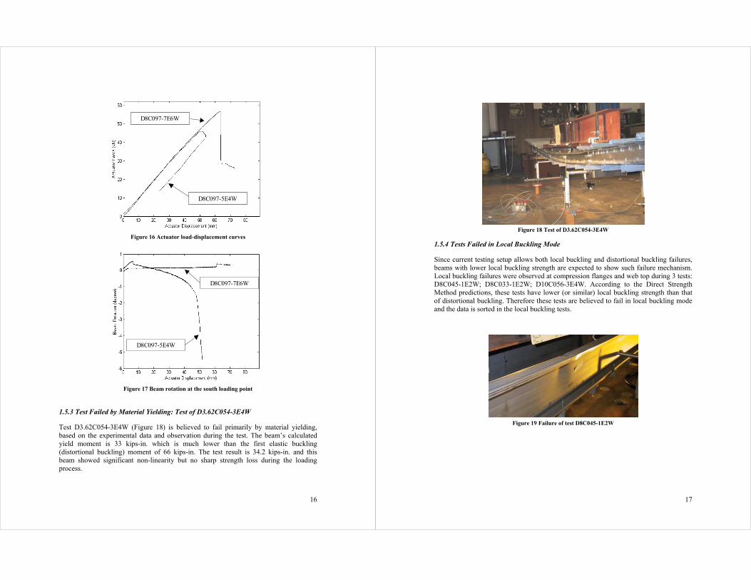
Elastic finite element analysis was performed to examine the new testing setup. After the angle is added to the compression flange the lateral-torsional buckling moment of D8C097-7E6W is increased from 589.5 kips-in., to 618.7 kips-in. Distortional buckling remains at almost the same value of 601.9 kips-in. Without the benefit of a nonlinear finite element analysis it was still decided to examine the experimental results with the angle attached. Figure 15 shows the failure mode of the new test (D8C097-7E6W) and Figure 16 shows the comparison of actuator load-displacement curves. The new test provided an increased strength and featured a distortional buckling failure mechanism. According to the Direct Strength Method calculation, the test-to-predicted result is increased from 84% for D8C097-5E4W to 99% for D8C097-7E6W. During the new test, the rotation and lateral movement observed in the previous test did not occur. One the other hand, the buckling happened at the compression flange which rotated against the web-flange junction. Deflection was also observed at the compression portion of web but it did not trigger the failure. Figure 17 shows the comparison of the rotation of beams at south loading point, the rotation angel is calculated according to the deflection data from two position transducers. It indicates the beam with standard setup had significant, continued increasing rotation during the test, but the beam with new setup had little rotation. Above all, test D8C097-7E6W is believed to fail in distortional buckling, and its data is included in subsequent analyses. D8C097-5E4W which provides an examination of the role of lateral-torsional buckling is not considered a distortional buckling test.
16
D8C097-5E4W
D8C097-7E6W
Figure 16 Actuator load-displacement curves
D8C097-5E4W
D8C097-7E6W
Figure 17 Beam rotation at the south loading point
1.5.3 Test Failed by Material Yielding: Test of D3.62C054-3E4W
Test D3.62C054-3E4W (Figure 18) is believed to fail primarily by material yielding, based on the experimental data and observation during the test. The beam’s calculated yield moment is 33 kips-in. which is much lower than the first elastic buckling (distortional buckling) moment of 66 kips-in. The test result is 34.2 kips-in. and this beam showed significant non-linearity but no sharp strength loss during the loading process.
17
Figure 18 Test of D3.62C054-3E4W
1.5.4 Tests Failed in Local Buckling Mode
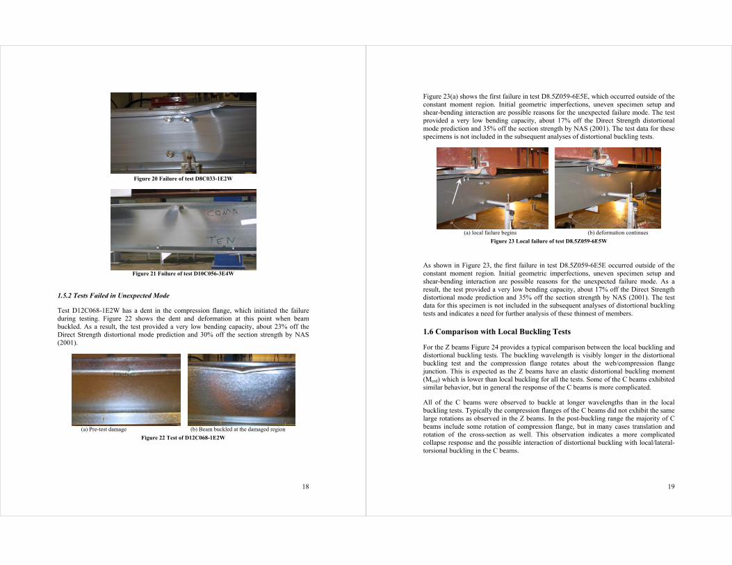
Since current testing setup allows both local buckling and distortional buckling failures, beams with lower local buckling strength are expected to show such failure mechanism. Local buckling failures were observed at compression flanges and web top during 3 tests: D8C045-1E2W; D8C033-1E2W; D10C056-3E4W. According to the Direct Strength Method predictions, these tests have lower (or similar) local buckling strength than that of distortional buckling. Therefore these tests are believed to fail in local buckling mode and the data is sorted in the local buckling tests.
Figure 19 Failure of test D8C045-1E2W
18
Figure 20 Failure of test D8C033-1E2W
Figure 21 Failure of test D10C056-3E4W
1.5.2 Tests Failed in Unexpected Mode
Test D12C068-1E2W has a dent in the compression flange, which initiated the failure during testing. Figure 22 shows the dent and deformation at this point when beam buckled. As a result, the test provided a very low bending capacity, about 23% off the Direct Strength distortional mode prediction and 30% off the section strength by NAS (2001).
(a) Pre-test damage (b) Beam buckled at the damaged region
Figure 22 Test of D12C068-1E2W
19
Figure 23(a) shows the first failure in test D8.5Z059-6E5E, which occurred outside of the constant moment region. Initial geometric imperfections, uneven specimen setup and shear-bending interaction are possible reasons for the unexpected failure mode. The test provided a very low bending capacity, about 17% off the Direct Strength distortional mode prediction and 35% off the section strength by NAS (2001). The test data for these specimens is not included in the subsequent analyses of distortional buckling tests.
(a) local failure begins (b) deformation continues
Figure 23 Local failure of test D8.5Z059-6E5W
As shown in Figure 23, the first failure in test D8.5Z059-6E5E occurred outside of the constant moment region. Initial geometric imperfections, uneven specimen setup and shear-bending interaction are possible reasons for the unexpected failure mode. As a result, the test provided a very low bending capacity, about 17% off the Direct Strength distortional mode prediction and 35% off the section strength by NAS (2001). The test data for this specimen is not included in the subsequent analyses of distortional buckling tests and indicates a need for further analysis of these thinnest of members.
1.6 Comparison with Local Buckling Tests
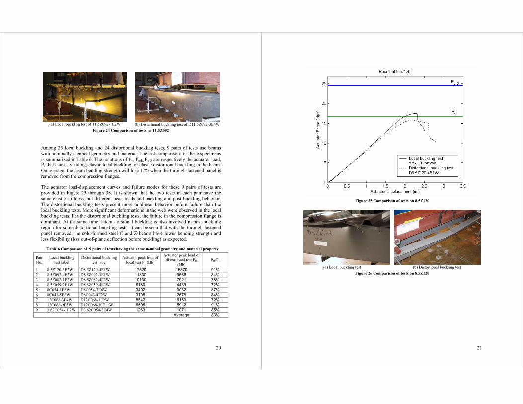
For the Z beams Figure 24 provides a typical comparison between the local buckling and distortional buckling tests. The buckling wavelength is visibly longer in the distortional buckling test and the compression flange rotates about the web/compression flange junction. This is expected as the Z beams have an elastic distortional buckling moment (Mcrd) which is lower than local buckling for all the tests. Some of the C beams exhibited similar behavior, but in general the response of the C beams is more complicated.
All of the C beams were observed to buckle at longer wavelengths than in the local buckling tests. Typically the compression flanges of the C beams did not exhibit the same large rotations as observed in the Z beams. In the post-buckling range the majority of C beams include some rotation of compression flange, but in many cases translation and rotation of the cross-section as well. This observation indicates a more complicated collapse response and the possible interaction of distortional buckling with local/lateral-torsional buckling in the C beams.
20
(a) Local buckling test of 11.5Z092-1E2W
(b) Distortional buckling test of D11.5Z092-3E4W
Figure 24 Comparison of tests on 11.5Z092
Among 25 local buckling and 24 distortional buckling tests, 9 pairs of tests use beams with nominally identical geometry and material. The test comparison for these specimens is summarized in Table 6. The notations of Py, PcrL, PcrD are respectively the actuator load, P, that causes yielding, elastic local buckling, or elastic distortional buckling in the beam. On average, the beam bending strength will lose 17% when the through-fastened panel is removed from the compression flanges.
The actuator load-displacement curves and failure modes for these 9 pairs of tests are provided in Figure 25 through 38. It is shown that the two tests in each pair have the same elastic stiffness, but different peak loads and buckling and post-buckling behavior. The distortional buckling tests present more nonlinear behavior before failure than the local buckling tests. More significant deformations in the web were observed in the local buckling tests. For the distortional buckling tests, the failure in the compression flange is dominant. At the same time, lateral-torsional buckling is also involved in post-buckling region for some distortional buckling tests. It can be seen that with the through-fastened panel removed, the cold-formed steel C and Z beams have lower bending strength and less flexibility (less out-of-plane deflection before buckling) as expected.
Table 6 Comparison of 9 pairs of tests having the same nominal geometry and material property
Pair No.
Local buckling test label
Distortional buckling test label
Actuator peak load of local test PL (klb)
Actuator peak load of distortional test PD
(klb) PD/PL
1 8.5Z120-3E2W D8.5Z120-4E1W 17520 15870 91% 2 8.5Z092-4E2W D8.5Z092-3E1W 11330 9566 84% 3 8.5Z082-1E2W D8.5Z082-4E3W 10130 7921 78% 4 8.5Z059-2E1W D8.5Z059-4E3W 6180 4439 72% 5 8C054-1E8W D8C054-7E6W 3492 3032 87% 6 8C043-5E6W D8C043-4E2W 3195 2678 84% 7 12C068-3E4W D12C068-1E2W 8542 6160 72% 8 12C068-9E5W D12C068-10E11W 6505 5912 91% 9 3.62C054-1E2W D3.62C054-3E4W 1263 1071 85% Average 83%
21
Figure 25 Comparison of tests on 8.5Z120
(a) Local buckling test (b) Distortional buckling test
Figure 26 Comparison of tests on 8.5Z120

22
Figure 27 Comparison of tests on 8.5Z092
(a) Local buckling test (b) Distortional buckling test
Figure 28 Comparison of tests on 8.5Z092
23
Figure 29 Comparison of tests on 8.5Z082
(a) Local buckling test (b) Distortional buckling test
Figure 30 Comparison of tests on 8.5Z082

24
Figure 31 Comparison of tests on 8.5Z059
(a) Local buckling test (b) Distortional buckling test
Figure 32 Comparison of tests on 8.5Z059
25
Figure 33 Comparison of tests on 8.5Z054
(a) Local buckling test (b) Distortional buckling test
Figure 34 Comparison of tests on 8.5Z054
Py

26
Figure 35 Comparison of tests on 8C043
(a) Local buckling test (b) Distortional buckling test
Figure 36 Comparison of tests on 8C043
27
Figure 37 Comparison of tests on 12C068
(a) Local buckling test (b) Distortional buckling test
Figure 38 Comparison of tests on 12C068

28
Figure 39 Comparison of tests on 12C068
(a) local buckling test (b)Distortional buckling test
Figure 40 Comparison of tests on 12C068
29
Figure 41 Comparison of tests on 3.62C054
(a) Local buckling test (b) Distortional buckling test
Figure 42 Comparison of tests on 3.62C054

30
1.7 Comparison with Current Design Specifications
Six design methods are considered for comparison: AISI (1996), S136 (1994), AS/NZS (1996), NAS (2001), EN1993 (2002) and DSM (2003). Specific specification predictions of the tested beams are listed in Table 5. Table 7 provides a summary of the test-to-predicted ratios. In average, all six methods give good strength predictions to the local buckling tests. DSM uses a single strength curve, while the other five methods apply effective width concepts in the calculation of bending strength. For the distortional buckling, only AS/NZS, EN1993 and DSM have specific equations for this mode. Table 7 shows that all three methods give good predictions to the tests, though the Eurocode predictions still remain about 5% unconservative on average. The Direct Strength Method has the best statistical results for any of the distortional buckling methods. AISI, S136 and NAS provide systematically unconservative predictions for the distortional buckling strength, the average error is between 10~15%. AISI (1996), S136 (1994) and NAS (2001) are only applicable to local buckling failures.
Table 7 Summary of test-to-predicted ratios for existing and proposed design methods
Mtest/ MAISI
Mtest/ MS136
Mtest/ MNAS
Mtest/ MAS/NZS
Mtest/ MEN1993
Mtest/ MDSM
µ 1.01 1.06 1.02 1.01 1.01 1.03 Controlling specimens σ 0.04 0.04 0.05 0.04 0.06 0.06
µ 1.00 1.05 1.01 1.00 1.01 1.03
Local buckling
tests Second specimens σ 0.05 0.06 0.07 0.05 0.06 0.07
µ 0.84 0.92 0.88 1.02 0.96 1.02 Controlling specimens σ 0.08 0.08 0.09 0.07 0.09 0.07
µ 0.85 0.90 0.87 1.00 0.94 1.00
Distortional buckling
tests Second specimens σ 0.08 0.07 0.09 0.07 0.09 0.07
DSM provides specific predictions for both local and distortional buckling of beams and is briefly summarized here. Since the beams are fully laterally braced, the maximum capacity due to long wavelength buckling Mne = My. For local buckling the capacity is:
776.0≤λ l , MDSl = My (1)
λl > 0.776, ( )( )( ) yMM
MM
DS MMy
cr
y
cr4.04.0
15.01 ll
l −= (2)
λl = lcry MM (3)
Where Mcrl = critical elastic local buckling moment and My = moment at first yield. For distortional buckling the capacity is:
673.0≤λd , MDSd = My (4)
λd > 0.673, ( )( )( ) yMM
MM
DSd MMy
crd
y
crd5.05.0
22.01−= (5)
λd= crdy MM (6)
31
Where Mcrd = Critical elastic distortional buckling moment. As shown in Table 7, the Direct Strength Method provides good agreement with both test series. The high test-to-predicted ratios for distortional buckling (Mtest/MDSd) in the local buckling tests indicate that distortional buckling was successfully restricted with the testing details employed in the Phase 1 testing. The overall agreement for MDSd in the distortional buckling tests indicates that distortional buckling dominated the failure mechanism when the compression flanges were unrestrained and validates the general expression used for distortional buckling in the DSM method (which was calibrated to other data).
Figure 43 provides a graphical representation of Equations 1 - 6 along with the results for both series tests. The average upper and lower bounds of laterally braced beams are well captured by the local and distortional buckling equations of the Direct Strength method. Local buckling test data are relatively more concentrated along the corresponding design curve than that of distortional buckling tests. The distortional buckling data show more deviation as the slenderness (My/Mcr ) increases.
Figure 43 Direct Strength Method vs. test results

32
2. Finite Element Modeling
2.1 Introduction
The experimental results build a solid background for further finite element analysis that can expand the buckling study to examine further cross sections, different loading and support conditions, and other structural details used in today’s industry. Elastic eigenvalue buckling analysis has already been used to determine the panel fastener configuration for local buckling tests. However, in order to simulate the real flexural bending tests, or to capture the buckling mechanism of cold-formed steel members, nonlinear inelastic finite element analysis is necessary.
2.2 Modeling Details and Boundary/Loading Conditions
The overall view of the finite element modeling is shown in Figure 44. The cold-formed steel purlins, panel and hot-rolled tubes are modeled using S4R shell element. The loading beam uses 8-node linear solid element (C3D8) and is simplified to be rectangular section.
lo a d in g p o in t
Figure 44 Finite element modeling of local buckling tests.
The beam is simply supported at the bottom flanges under the two end tubes. The tube and purlin is connected by imposing 4 nodes (to simulate the four bolts) of the purlin to the surface of the tube. ABAQUS provides a Multi-Point Constraints (*MPC in ABAQUS) library for different connection/contact modeling. The “*Tie” option is used for the tube-to-purlin connection (Figure 45), that is to make the global displacements and rotations as well as all other active degrees of freedom equal at two nodes. The same method is also employed for the panel-to-purlin connection (Figure 46). The loading beam is simply connected to the tubes (Figure 45) using *Pin option in ABAQUS, that makes the global displacements equal but leaves the rotations, if they exist, independent
33
of each other. The angle at the bottom of the purlins is simulated by keeping the distance between two nodes on the tension flanges constant (Figure 47) (*Link in ABAQUS).
Solid element (C3D8)Shell element (S4R)
Pin connection between Load
beam and tube
Tie connection between purlin
and tube
Solid element (C3D8)Shell element (S4R)
Pin connection between Load
beam and tube
Tie connection between purlin
and tube
Figure 45 Connections at the 1/3 point of beams
Shell element (S4R) Tie connection between purlin
and panel
Shell element (S4R) Tie connection between purlin
and panel
Figure 46 Panel-to-purlin connection
two nodes linked
Figure 47 Modeling of angles at the tension flanges (view from under the beam)
The material nonlinearity is one of the primary nonlinearity considerations for the postbuckling analysis of cold-formed steel members. Since the Z and C purlins are the research objectives, only purlins are modeled as inelastic material (note, typical yield stress for the panel is quite high, about 100 ksi, and failures were observed to initiate in the members, not the panels, for all local and distortional buckling tests).
34
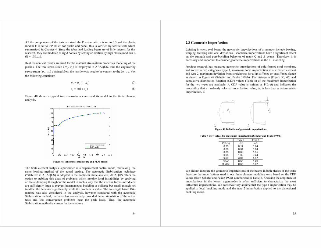
All the components of the tests are steel, the Possion ratio v is set to 0.3 and the elastic moduli E is set to 29500 ksi for purlin and panel, this is verified by tensile tests which summarized in Chapter 4. Since the tubes and loading beam are of little interest for this research, they are modeled as rigid bodies by setting an artificially high elastic modulus E (E = 10Esteel).
Real tension test results are used for the material stress-strain properties modeling of the purlins. The true stress-strain ( eσ , eε ) is employed in ABAQUS, thus the engineering
stress-strain ( tσ , tε ) obtained from the tensile tests need to be convert to the ( eσ , eε ) by
the following equations:
)1( eet εσσ += (7)
)1ln( et εε += (8)
Figure 48 shows a typical true stress-strain curve and its model in the finite element analysis.
Figure 48 True stress-strain cure and FEM model
The finite element analysis is performed in a displacement control mode, mimicking the same loading method of the actual testing. The automatic Stabilization technique (*stabilize in ABAQUS) is adopted in the nonlinear static analysis, ABAQUS offers the option to stabilize this class of problems which involve local instabilities by applying artificial damping throughout the model in such a way that the viscous forces introduced are sufficiently large to prevent instantaneous buckling or collapse but small enough not to affect the behavior significantly while the problem is stable. The arc-length based Riks method was also considered in the analysis, however compared with the automatic Stabilization method, the latter has consistently provided better simulation of the actual tests and less convergence problems near the peak loads. Thus, the automatic Stabilization method is chosen for the analyses.
35
2.3 Geometric Imperfection
Existing in every real beam, the geometric imperfections of a member include bowing, warping, twisting and local deviations. Geometric imperfections have a significant effect on the strength and post-buckling behavior of many C and Z beams. Therefore, it is necessary and important to consider geometric imperfections in the FE modeling.
Previous research has measured geometric imperfections of cold-formed steel members, and sorted in two categories: type 1, maximum local imperfection in a stiffened element and type 2, maximum deviation from straightness for a lip stiffened or unstiffened flange as shown in Figure 49 (Schafer and Peköz 1998b). The histogram (Figure 50, 46) and cumulative distribution function (CDF) values (Table 8) of the maximum imperfection for the two types are available. A CDF value is written as P(∆<d) and indicates the probability that a randomly selected imperfection value, ∆, is less than a deterministic imperfection, d.
d
1
1
d
2
2
Figure 49 Definition of geometric imperfections
Table 8 CDF values for maximum imperfection (Schafer and Peköz 1998b)
Type 1 Type 2 P(∆<d) d1/t d2/t 0.25 0.14 0.64 0.50 0.34 0.94 0.75 0.66 1.55 0.95 1.35 3.44 0.99 3.87 4.47 mean 0.50 1.29
st. dev. 0.66 1.07
We did not measure the geometric imperfections of the beams in both phases of the tests; therefore the imperfections used in our finite element modeling were based on the CDF values (from Schafer and Peköz 1998) summarized in Table 8. Knowing the amplitude of imperfections in the lowest eigenmodes is often sufficient to characterize the most influential imperfections. We conservatively assume that the type 1 imperfection may be applied to local buckling mode and the type 2 imperfection applied to the distortional buckling mode.

36
0 1 2 3 4 50
5
10
15
20
25
30
35
40
45
d/t
num
ber
of o
bser
vati
ons
0 1 2 3 4 5 6 7
0
5
10
15
20
25
30
35
d/t
num
ber
of o
bser
vati
ons
Figure 50 Histogram of type 1 imperfection
(Schafer and Peköz 1998b) Figure 51 Histogram of type 2 imperfection
(Schafer and Peköz 1998b)
For each test two different magnitudes of geometric imperfections are generated, the first uses a 25% CDF maximum magnitude, and the second a 75% CDF imperfection, thus covering the middle 50% of anticipated imperfection magnitudes. The imperfection shape is a superposition of the local and distortional buckling mode scaled to the appropriate CDF value. For numerical efficiency the buckling shape is obtained by using finite strip analysis in CUFSM and the resulting coordinates used to offset the geometry of the ABAQUS model appropriately.
2.4 Residual Stress
Unlike hot-rolled steel members, residual stresses in cold-formed members are dominated by a flexural, or through thickness variation in the residual stress. This variation of residual stresses leads to early yielding on the faces of cold-formed steel elements. However it is difficult to include the residual stress in the model and more important, the experimental result is in great shortage. The experimentally measuring the through thickness variation of a thin plate is even not practical currently.
The residual stress is not directly measured in the tests. The material properties of the flanges and webs were measured by the tensile tests, but no difference of the strength is observed. Therefore the residual stress is not considered in the finite element modeling in this research.
2.5 Comparison with Experimental Results
For each test, two nonlinear finite element analyses are performed, one FEM model use the imperfection with 25% CDF maximum magnitude and the other one uses the imperfection with 75% CDF thus covering the middle 50% of anticipated imperfection magnitudes. The imperfection shape is obtained by superposing the local and distortional buckling mode, scaled to the appropriate CDF value. For numerical efficiency, the finite strip analysis by CUFSM is used to generate the buckling shapes.
Figure 52 shows the comparison of the local buckling test result of 11.5Z092-1E2W with the result of finite element model with 25% CDF imperfection. Figure 53 shows the
37
comparison of the distortional buckling test result of D11.5Z092-3E4W with the result of finite element model with 25% CDF imperfection. It can be seen the ABAQUS gives good prediction of the buckling shapes for both tests: the local buckling tests is characterized by short and repeated buckling waves at the compression flange and the top portion of the web; the test without the restraint by panel fails in a typical distortional buckling mode that is the compression flange rotates with longer wavelength than local mode.
(a) FEM result (loading beam removed for better view)
(b) Test result
Figure 52 Local buckling test of 11.5Z092-1E2W
(a) FEM result (loading beam removed for better view)
(b) Test result
Figure 53 Distortional buckling test of D11.5Z092-3E4W

38
The finite element analysis results are summarized in Table 9 for the local buckling tests and Table 10 for the distortional buckling tests. On average, the failure load is bounded by the two finite element simulations with 25% and 75% CDF maximum imperfections. The pair of simulations show that the middle 50% of imperfections exhibit a range of 14% of the bending capacity, thus providing a measure of the imperfection sensitivity. Average test-to-predicted ratios for the finite element analysis of the local buckling tests are closer to 1 (100%) than the distortional buckling tests. The finite element analysis for the distortional buckling tests shows slightly greater scatter (greater imperfection sensitivity) and the mean response of the FE simulations is slightly greater than the average tested strength. Figure 54 shows the FEM accuracy vs. web slenderness, and indicates a slight tendency for the finite element analysis to over-predict the observed strength for very slender sections and under-predict for stockier sections. This may be partially driven by the choice of a constant d/t imperfection size – thus leading to smaller imperfection sizes for the more slender members which typically employ thinner material.
0
0.2
0.4
0.6
0.8
1
1.2
1.4
0.4 0.6 0.8 1 1.2 1.4 1.6 1.8 2
web slenderness = λweb = (fy/fcr_web)0.5
FE
M-t
o-t
est
ra
tio
25% CDF
75% CDF
Figure 54 Comparison of finite element results with tests
In total it is concluded that the elastic, post-buckling, and peak strength behavior of the beams are well simulated by this finite element model and its assumptions. However, the post-collapse behavior and final mechanism formation is only approximated by the model. Lack of agreement in the large deflection post-collapse range could be a function of the solution scheme (e.g., use of artificial damping via the *stabilize option) or more basic modeling assumptions, such as ignoring any plasticity in the panels. Load-deflection response for six of the approximately 8 in. deep sections is given in Figure 55.
39
Table 9 Summary of finite element analysis results for local buckling tests
Ptest(lbs) P25% P25%/Ptest P75%(lbs) P75%/Ptest
8.5Z120-3E2W 17520 17968 103% 16484 94% 8.5Z105-2E1W 16720 17294 103% 15806 95% 8.5Z092-4E2W 11330 11901 105% 11170 99% 8.5Z082-1E2W 10130 11446 113% 10749 106% 8.5Z073-4E3W 8341 8770 105% 7309 88% 8.5Z065-3E1W 5969 6771 113% 5886 99% 8.5Z059-2E1W 6180 6749 109% 5748 93% 11.5Z073-2E1W 12120 13956 115% 12396 102% 11.5Z082-2E1W 17123 17294 101% 15806 92% 11.5Z092-1E2W 22000 23417 106% 19790 90% 8.5Z059-4E3W 6275 6855 109% 5763 92% 8C097-2E3W 10770 11175 104% 10200 95% 8C068-4E5W 6476 6762 104% 5614 87% 8C054-1E8W 3492 3849 110% 3233 93% 8C043-5E6W 3195 3574 112% 3082 96% 6C054-2E1W 2803 2882 103% 2240 80% 4C054-1E2W 1731 1720 99% 1365 79% 12C068-9E5W 6505 6697 103% 5968 92% 3.62C054-1E2W 1263 1170 93% 987 78% 12C068-3E4W 8542 9458 111% 8655 101% 10C068-2E1W 4381 4233 97% 3937 90% 8C068-1E2W 6141 6854 112% 5557 90% 8C043-3E1W 2985 3482 117% 3026 101%
mean 106% 93% standard deviation 6% 7%
Note: Ptest: Peak tested actuator load P25%: Peak load of simulation with 25% CDF of maximum imperfection P75%: Peak load of simulation with 75% CDF of maximum imperfection

40
Table 10 Summary of finite element analysis results for distortional buckling tests
Test Label Ptest(lbs) P25% P25%/Ptest P75%(lbs) P75%/Ptest
D8.5Z120-4E1W 15870 16283 103% 14839 94%
D8.5Z115-1E2W 14837 16402 111% 13028 88%
D8.5Z092-3E1W 9566 10740 112% 8779 92%
D8.5Z082-4E3W 7921 9160 116% 7775 98%
D8.5Z065-7E6W 5826 6891 118% 6053 104%
D11.5Z092-3E4W 16377 16817 103% 14443 88%
D8.5Z065-4E5W 4993 5876 118% 5155 103%
D11.5Z082-4E3W 14578 15172 104% 14473 99%
D12C068-1E2W 6160 8157 132% 7566 123%
D8C043-4E2W 2678 3051 114% 2751 103%
D12C068-10E11W 5912 5497 93% 4930 83%
D8C033-1E2W 1024 1089 106% 950.8 93%
D8C054-7E6W 3032 3363 111% 2919 96%
D10C068-4E3W 3185 3235 102% 2746 86%
D8C097-5E4W 10350 12353 119% 9985 96%
D3.62C054-3E4W 1071 1027 96% 838 78%
D8C097-7E6W 12751 13690 107% 10771 84%
D10C048-1E2W 3874 4228 109% 3806 98%
D8C045-1E2W 1033 1134 110% 1023 99%
D6C063-2E1W 3271 3537 108% 2992 91%
D8C085-2E1W 7646 7723 101% 6677 87%
D10C056-3E4W 5309 7723 109% 5003 94%
D8C068-6E7W 6553 6829 104% 6211 95%
mean 109% 94%
standard deviation 8% 9% Note: Ptest: Peak tested actuator load
P25%: Peak load of simulation with 25% CDF of maximum imperfection P75%: Peak load of simulation with 75% CDF of maximum imperfection
41
Figure 55 Comparison of selected tests with finite element analysis results

42
2.6 Extended Finite Element Analysis
After being verified by the real tests, the finite element analysis can be extended to other practical sections which are not included in both series tests. The maximum imperfection of 50% CDF ( 34.0/1 =td , 94.0/2 =td ) is applied in the extended finite element simulations and typical stress-strain curves obtained from tensile tests are applied for the material model in FEA. Based on the statistical results of finished FE analyses, the 50% CDF simulation, on average, will give strength predictions within an error of 7% of the real values for local buckling tests and 9% for the distortional buckling tests.
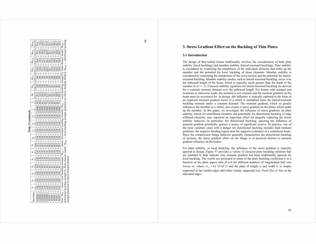
The completed FEA results and section geometry are summarized in Table 11. The geometry is chosen from industry standard cold-formed steel section and the tested specimens in the experimental work. Each geometry section is applied five different level strengths of material; the yielding stresses are 33 ksi, 44 ksi, 56.1 ksi, 62.2 ksi and 73.4 ksi. Figure 56 shows the comparison of FEA results with the Direct Strength predications. It indicates that the direct strength method provides conservative but pretty reasonable predictions for both local and distortional buckling strengths. The distortional buckling prediction gives good agreement with the FEA results. The local buckling
strengths for the unslender sections ( ( ) 8.0/ 5..0 <cry MM ) becomes is more scattered and
the Direct Strength Method tends to give unconservative predictions for some beams at this region.
Figure 56 FEA results vs. DSM predications
43
Tab
le 1
1 S
ecti
on d
imen
sion
s an
d r
esu
lts
of e
xten
ded
fin
ite
elem
ent
anal
ysis
Spe
cim
en
h (in.
) b c
(i
n.)
d c
(in.
) θ c
(d
eg)
b t
(in.
) d t
(i
n.)
θ t
(deg
) r h
c (i
n.)
r dc
(in.
) r h
t (i
n.)
r dt
(in.
) t
(in.
) f y
(k
si)
My
(kip
s-in
.)
Mcf
L
(kip
s-in
.)M
crD
(k
ips-
in.)
MF
EL
(k
ips-
in.)
MF
ED
(k
ips-
in)
MD
SL
(k
ips-
in)
MD
SD
(k
ips-
in)
8Z2.
25x0
50
8.0
2.3
0.9
50
2.3
0.9
50
0.24
0.
24
0.24
0.
24
0.05
00
33
54.7
56
.1
58.5
52
.8
48.2
47
44
8Z
2.25
x050
8.
0 2.
3 0.
9 50
2.
3 0.
9 50
0.
24
0.24
0.
24
0.24
0.
0500
44
72
.9
56.1
58
.5
65.9
58
.6
57
52
8Z2.
25x0
50
8.0
2.3
0.9
50
2.3
0.9
50
0.24
0.
24
0.24
0.
24
0.05
00
56.1
93
.0
56.1
58
.5
79.1
67
.6
67
61
8Z2.
25x0
50
8.0
2.3
0.9
50
2.3
0.9
50
0.24
0.
24
0.24
0.
24
0.05
00
62.2
10
3.2
56.1
58
.5
83.5
70
.6
71
65
8Z2.
25x0
50
8.0
2.3
0.9
50
2.3
0.9
50
0.24
0.
24
0.24
0.
24
0.05
00
73.4
12
1.7
56.1
58
.5
89.6
76
.0
79
71
8Z2.
25x1
00
8.0
2.3
0.9
50
2.3
0.9
50
0.24
0.
24
0.24
0.
24
0.05
00
33
106.
2 43
8.0
26
1.5
11
4.2
114.
2 10
6 10
6 8Z
2.25
x100
8.
0 2.
3 0.
9 50
2.
3 0.
9 50
0.
24
0.24
0.
24
0.24
0.
0500
44
14
1.6
438.
0
261.
5
145.
6 13
6.4
142
135
8Z2.
25x1
00
8.0
2.3
0.9
50
2.3
0.9
50
0.24
0.
24
0.24
0.
24
0.05
00
56.1
18
0.6
438.
0
261.
5
180.
3 16
5.5
181
160
8Z2.
25x1
00
8.0
2.3
0.9
50
2.3
0.9
50
0.24
0.
24
0.24
0.
24
0.05
00
62.2
20
0.3
438.
0
261.
5
189.
1 17
3.3
200
171
8Z2.
25x1
00
8.0
2.3
0.9
50
2.3
0.9
50
0.24
0.
24
0.24
0.
24
0.05
00
73.4
23
6.3
438.
0
261.
5
214.
1 19
6.0
236
191
8.5Z
2.6
x70
8.5
2.5
0.9
50
2.5
0.9
50
0.25
0.
25
0.25
0.
25
0.07
00
73.4
19
3.2
152.
3
119.
4
157.
1 13
6.3
152
126
8.5Z
2.6
x70
8.5
2.5
0.9
50
2.5
0.9
50
0.25
0.
25
0.25
0.
25
0.07
00
62.2
16
3.8
152.
3
119.
4
142.
6 12
4.2
136
114
8.5Z
2.6
x70
8.5
2.5
0.9
50
2.5
0.9
50
0.25
0.
25
0.25
0.
25
0.07
00
56.1
14
7.6
152.
3
119.
4
135.
5 11
9.0
127
107
8.5Z
2.6
x70
8.5
2.5
0.9
50
2.5
0.9
50
0.25
0.
25
0.25
0.
25
0.07
00
44
115.
8 15
2.3
11
9.4
11
1.2
100.
1 10
8 91
8.
5Z2.
6x7
08.
5 2.
5 0.
9 50
2.
5 0.
9 50
0.
25
0.25
0.
25
0.25
0.
0700
33
86
.8
152.
3
119.
4
87.9
81
.7
87
76
11.5
Z3.
5x8
0 11
.5
3.5
0.9
50
3.5
0.9
50
0.30
0.
30
0.30
0.
30
0.08
00
33
179.
5 22
1.9
16
9.9
17
1.3
152.
4 16
4 13
7 11
.5Z
3.5
x80
11.5
3.
5 0.
9 50
3.
5 0.
9 50
0.
30
0.30
0.
30
0.30
0.
0800
44
23
9.4
221.
9
169.
9
212.
7 18
2.6
198
164
11.5
Z3.
5x8
0 11
.5
3.5
0.9
50
3.5
0.9
50
0.30
0.
30
0.30
0.
30
0.08
00
56.1
30
5.3
221.
9
169.
9
255.
5 21
3.0
233
190
11.5
Z3.
5x8
0 11
.5
3.5
0.9
50
3.5
0.9
50
0.30
0.
30
0.30
0.
30
0.08
00
62.2
33
8.6
221.
9
169.
9
267.
6 22
4.3
250
202
11.5
Z3.
5x8
0 11
.5
3.5
0.9
50
3.5
0.9
50
0.30
0.
30
0.30
0.
30
0.08
00
73.4
39
9.5
221.
9
169.
9
292.
7 24
2.5
278
223
8C06
8-6
7.9
1.9
0.7
80
2.0
0.6
77.8
0.
16
0.16
0.
16
0.16
0.
0700
33
65
.2
134.
3
136.
3
69.4
63
.7
65
64
8C06
8-6
7.9
1.9
0.7
80
2.0
0.6
77.8
0.
16
0.16
0.
16
0.16
0.
0700
44
86
.9
134.
3
136.
3
87.5
79
.4
85
79
8C06
8-6
7.9
1.9
0.7
80
2.0
0.6
77.8
0.
16
0.16
0.
16
0.16
0.
0700
56
.1
110.
8 13
4.3
13
6.3
10
7.2
97.1
10
0 93
8C
068-
6 7.
9 1.
9 0.
7 80
2.
0 0.
6 77
.8
0.16
0.
16
0.16
0.
16
0.07
00
62.2
12
2.9
134.
3
136.
3
112.
5 10
1.8
108
99
8C06
8-6
7.9
1.9
0.7
80
2.0
0.6
77.8
0.
16
0.16
0.
16
0.16
0.
0700
73
.4
145.
0 13
4.3
13
6.3
11
5.1
115.
1 12
0 11
1 8.
5Z09
2-2
8.
4 2.
6 0.
9 51
.8
2.4
1.0
50.4
0.
28
0.28
0.
31
0.31
0.
0900
33
10
8.0
332.
7
208.
9
117.
2 10
9.5
108
104
8.5Z
092
-3
8.4
2.6
0.9
51.8
2.
4 1.
0 50
.4
0.28
0.
28
0.31
0.
31
0.09
00
44
144.
1 33
2.7
20
8.9
14
9.3
136.
6 14
4 12
8 8.
5Z09
2-4
8.
4 2.
6 0.
9 51
.8
2.4
1.0
50.4
0.
28
0.28
0.
31
0.31
0.
0900
56
.1
183.
7 33
2.7
20
8.9
18
5.4
165.
9 18
4 15
0 8.
5Z09
2-5
8.
4 2.
6 0.
9 51
.8
2.4
1.0
50.4
0.
28
0.28
0.
31
0.31
0.
0900
62
.2
203.
7 33
2.7
20
8.9
19
4.0
172.
8 20
3 16
0 8.
5Z09
2-6
8.
4 2.
6 0.
9 51
.8
2.4
1.0
50.4
0.
28
0.28
0.
31
0.31
0.
0900
73
.4
240.
3 33
2.7
20
8.9
22
1.1
193.
2 22
7 17
8 8.
5Z12
0-2
8.
5 2.
6 1.
0 47
.8
2.5
1.0
48.9
0.
36
0.36
0.
34
0.34
0.
1176
33
14
2.6
728.
9
365.
5
155.
6 14
9.7
143
143
8.5Z
120
-2
8.5
2.6
1.0
47.8
2.
5 1.
0 48
.9
0.36
0.
36
0.34
0.
34
0.11
76
44
190.
2 72
8.9
36
5.5
19
8.2
190.
3 19
0 18
3 8.
5Z12
0-2
8.
5 2.
6 1.
0 47
.8
2.5
1.0
48.9
0.
36
0.36
0.
34
0.34
0.
1176
56
.1
242.
5 72
8.9
36
5.5
24
5.7
236.
2 24
2 21
7 8.
5Z12
0-2
8.
5 2.
6 1.
0 47
.8
2.5
1.0
48.9
0.
36
0.36
0.
34
0.34
0.
1176
62
.2
268.
9 72
8.9
36
5.5
25
8.3
248.
1 26
9 23
3 8.
5Z12
0-2
8.
5 2.
6 1.
0 47
.8
2.5
1.0
48.9
0.
36
0.36
0.
34
0.34
0.
1176
73
.4
317.
3 72
8.9
36
5.5
29
3.0
283.
3 31
7 26
0
44
T
able
11
(con
tin
ued
)
Spe
cim
enh (in.
) b c
(i
n.)
d c
(in.
) θ c
(d
eg)
b t
(in.
) d t
(i
n.)
θ t
(deg
) r h
c (i
n.)
r dc
(in.
) r h
t (i
n.)
r dt
(in.
) t
(in.
) f y
(k
si)
My
(kip
s-in
.)
Mcf
L
(kip
s-in
.)
Mcr
D
(kip
s-in
.)M
FE
L
(kip
s-in
.)
MF
ED
(k
ips-
in)
MD
SL
(k
ips-
in)
MD
SD
(k
ips-
in)
8.5Z
082
-1
8.46
2.
50
0.95
49
.0
2.36
0.
97
50.3
0.
28
0.28
0.
30
0.30
0.
0806
33
.0
97.0
23
6 16
4 10
3.2
94.8
97
.0
91.2
8.
5Z08
2-1
8.
46
2.50
0.
95
49.0
2.
36
0.97
50
.3
0.28
0.
28
0.30
0.
30
0.08
06
44.0
12
9.3
236
164
130.
6 11
6.9
129.
3 11
3.2
8.
5Z08
2-1
8.
46
2.50
0.
95
49.0
2.
36
0.97
50
.3
0.28
0.
28
0.30
0.
30
0.08
06
56.1
16
4.9
236
164
161.
2 14
1.3
164.
9 13
6.0
8.
5Z08
2-1
8.
46
2.50
0.
95
49.0
2.
36
0.97
50
.3
0.28
0.
28
0.30
0.
30
0.08
06
62.2
18
2.8
236
164
169.
6 14
7.3
179.
8 14
7.2
8.
5Z08
2-1
8.
46
2.50
0.
95
49.0
2.
36
0.97
50
.3
0.28
0.
28
0.30
0.
30
0.08
06
73.4
21
5.7
236
164
204.
2 16
4.4
205.
6 16
7.6
8C
097-
1 8.
04
2.09
0.
58
85.1
2.
07
0.53
86
.3
0.28
0.
28
0.29
0.
28
0.09
80
33.0
90
.1
361
258
98.1
92
.3
90.1
90
.1
8C09
7-1
8.04
2.
09
0.58
85
.1
2.07
0.
53
86.3
0.
28
0.28
0.
29
0.28
0.
0980
44
.0
120.
1 36
1 25
8 12
4.6
118.
0 12
0.1
120.
1
8C09
7-1
8.04
2.
09
0.58
85
.1
2.07
0.
53
86.3
0.
28
0.28
0.
29
0.28
0.
0980
56
.1
153.
1 36
1 25
8 15
4.6
140.
6 15
3.1
148.
0
8C09
7-1
8.04
2.
09
0.58
85
.1
2.07
0.
53
86.3
0.
28
0.28
0.
29
0.28
0.
0980
62
.2
169.
8 36
1 25
8 16
2.9
148.
3 16
9.8
160.
7
8C09
7-1
8.04
2.
09
0.58
85
.1
2.07
0.
53
86.3
0.
28
0.28
0.
29
0.28
0.
0980
73
.4
200.
3 36
1 25
8 18
4.9
162.
8 20
0.3
183.
8
Not
e: M
cfL
---
elas
tic l
ocal
buc
klin
g m
omen
t; M
cfD
---
elas
tic d
isto
rtio
nal
buck
ling
mom
ent;
MF
EL
---
loca
l bu
cklin
g st
reng
th b
y fi
nite
ele
men
t m
odel
; M
FE
D --
- di
stor
tiona
l bu
cklin
g st
reng
th b
y fi
nite
ele
men
t m
odel
; M
DS
L -
-- l
ocal
buc
klin
g st
reng
th p
redi
ctio
n by
Dir
ect
Str
engt
h M
etho
d; M
DS
D -
-- d
isto
rtio
nal
buck
ling
st
reng
th p
redi
ctio
n by
Dir
ect S
tren
gth
Met
hod.
45
3. Stress Gradient Effect on the Buckling of Thin Plates
3.1 Introduction
The design of thin-walled beams traditionally involves the consideration of both plate stability (local buckling) and member stability (lateral-torsional buckling). Plate stability is considered by examining the slenderness of the individual elements that make up the member and the potential for local buckling of those elements. Member stability is considered by examining the slenderness of the cross-section and the potential for lateral-torsional buckling. Member stability modes, such as lateral-torsional buckling, occur over the unbraced length of the beam, which is typically much greater than the depth of the member (L/d >> 1). Classical stability equations for lateral-torsional buckling are derived for a constant moment demand over the unbraced length. For beams with unequal end moments or transverse loads, the moment is not constant and the moment gradient on the beam must be accounted for. In design, this influence is typically captured in the form of an empirical moment gradient factor (Cb) which is multiplied times the lateral-torsional buckling moment under a constant demand. The moment gradient, which so greatly influences the member as a whole, also creates a stress gradient on the plates which make up the member. In this paper, we investigate the influence of stress gradients on plate stability, which for unstiffened elements and potentially for distortional buckling of edge stiffened elements, may represent an important effect for properly capturing the actual stability behavior. In particular, for distortional buckling, ignoring the influence of moment gradient potentially ignores a source of significant reserve. In practice, one of the most common cases with a danger for distortional buckling includes high moment gradients: the negative bending region near the supports (columns) of a continuous beam. Since the compression flange behavior generally characterizes the distortional buckling of sections, the stress gradient effect on the flange is of practical interest to moment gradient influence on the beams.
For plate stability, or local buckling, the influence of the stress gradient is typically ignored in design. Figure 57 provides a variety of classical plate buckling solutions that are intended to help indicate why moment gradient has been traditionally ignored for local buckling. The results are presented in terms of the plate buckling coefficient k as a function of the plate aspect ratio β=a/b for different numbers of longitudinal half sine waves, m. where: )/( 22 tbDkcr πσ = and the plate of length a, and width b, is simply
supported at the loaded edges and either simply supported (ss), fixed (fix) or free at the unloaded edges.

46
β
k
ss ss fix
fix m=1 m=2 m=3 m=4 m=5 m=6 m=7 m=8 m=9 m=10
m=1 m=2 m=3 m=4 m=5 m=6 m=7
m=1 m=2 m=3 m=4
m=1
ss ss
ss
ss
ss ss fix
free
ss ss ss
free
m=2 m=3
Figure 57 Buckling of uniformly compressed rectangular plates
Figure 57 indicates that when the unloaded edges are supported, the length of the buckled wave is quite short and many buckled waves (high m) can form in even relatively short lengths. When one of the unloaded edges is unsupported (e.g. fix-free) the behavior is modified from the supported case and now even at relatively large β values the number of expected half-waves (m) are small. The behavior of the ss-free case is particularly interesting. Instead of the distinct garland curves of the earlier cases, now for higher β, the single half-wave case (m=1) asymptotes to k=0.425 instead of increasing for large β. For the ss-free case multiple wavelengths (m) all yield similar solutions for large β.
To connect the plate solutions of Figure 1 to actual beams, consider the top flanges of the beams of Figure 58. Local buckling of the compression flange of the hat of Figure 58(a) is somewhere between the ss-ss and fix-fix case of Figure 57. What would be the influence of moment gradient on the local buckling of the compression flange in this solution? One anticipates that even a sharply varying moment gradient is unlikely to change the stress demands on the flange significantly. Therefore, traditional local buckling of a stiffened element – such as the compression flange of the hat – is assumed to not require modification due to the moment gradient. However, now consider the channel of Figure 58(b). As the compression flange buckles the web/flange juncture provides support somewhere between the fix-free and ss-free case of Figure 57. The potential that moment gradient may have influence on the buckling results is real. Further, and somewhat counter-intuitively, the weaker the support on the unloaded edge, the greater the potential for an increase in the buckling load due to the moment gradient.
47
(a) hat section (b) channel section
Figure 58 Section shapes
Channel sections with unstiffened flanges such as that of Figure 58(b) are widely used in practice. Finite strip analysis (FSA) provides a means to examine the plate stability and member stability within one solution. Figure 59 gives a typical FSA result for a 9 in. deep, 4 in. wide C section (with t=0.04 in.) subject to bending moment. The y axis is a multiplier times the applied moment (load factor) which indicates the magnitude of the elastic buckling moment, and the x axis is the half wavelength in inches.
100
101
102
103
0
10
20
30
40
50
60
70
80
90
half−wavelength (in.)
load
fact
or
Distortional Lateral-torsional
Figure 59 Finite strip result of the buckling of C section in bending
It is the convention of the authors to term buckling modes that occur at half-wavelengths greater than the largest dimension of the member in compression as distortional buckling. Thus, the “local buckling” of the fix-free and ss-free cases presented in Figure 1 would be termed distortional. Our definition of distortional buckling provides a necessary distinction for lipped channels, where local buckling does not involve translation of the fold-lines of a cross-section, but only rotation. The FSA results show that distortional buckling involves rotation of the compression flange about the web-flange juncture while lateral-torsional buckling involves translation and rotation of the entire section, without any distortion of the cross-section itself. Distortional buckling occurs at about a 10 in. half wavelength, which is relatively long compared to the flange width. Therefore, the influence of moment gradient on the buckling of this section may be of practical interest.

48
3.2 Analytic Solution: Energy Method
To investigate the influence of stress gradient on plate stability we will consider the buckling of stiffened (Figure 60) and unstiffened (Figure 61) elements via the Rayleigh-Ritz method. As shown in Figure 60 and Figure 61, we consider unequal stresses applied at the ends to account for the influence of moment gradient on the applied stress for a plate isolated from the member.
o
Y
min σ maxσ
τ
a
b simply supported
X
τ
τ τ
Figure 60 Stiffened element subject to a stress gradient
o
Y
min σ max σ
τ
a
b
free edge
elastic restrained edge τ τ
X
Figure 61 Unstiffened element subject to a stress gradient
The Rayleigh-Ritz method has been widely applied to determine the buckling stress of plates. In this method, an assumed deflection function satisfying the boundary conditions is used in the expression for the total potential energy Π . The total potential energy is the summation of internal strain energy U of the plate during bending, and the work done by the external forces T. Classical solutions from thin plate theory (e.g. Timoshenko and Gere 1961) result in:
TU +=Π (9)
49
dxdyyx
w
y
w
x
w
y
w
x
wDU
b a
∫ ∫
∂∂
∂−
∂∂
∂∂
−−
∂∂
+∂∂
=0 0
22
2
2
2
22
2
2
2
2
)1(22
µ (10)
∫ ∫
∂∂
∂∂
+
∂∂
+
∂∂
−=b a
xyyx dxdyy
w
x
w
y
w
x
wtT
0 0
22
22
τσσ (11)
Using the principle of minimum total potential energy, the equilibrium configuration of the plate is identified by Equations (12).
( )Niwi
K2,10 ==∂
Π∂ (12)
Equation (12) represents a system of N simultaneous homogeneous equations with iw
and load σ (σmax is used in present paper) as unknowns. For nontrivial solution of iw ’s,
the determinant of the coefficient matrix of the system of equations must vanish. The lowest value of σmax that leaves the determinant of the coefficient matrix to be zero is the critical load of the plate.
3.3 Stress Gradient on Stiffened Elements
Earlier work of Libove, Ferdman and Reusch (1949) considered the influence of stress gradient on a simply supported rectangular plate (ss-ss) of uniform thickness. The plate is shown in Figure 4. The distribution of compressive stress in the plate is assumed to be linear in the loading (longitudinal) direction. The difference between the compressive stresses at the two loaded edges is equilibrated by shear stresses along the unloaded edges. The Rayleigh-Ritz method is used to obtain the buckling stresses and a double Fourier sin series is employed as the assumed deflection function:
∑∑= =
=M
m
N
nmn b
yn
a
xmww
1 1
sinsinππ
, (13)
Via (12) the equilibrium equations are derived as Equation (14) (same as Equation A11 in Libove, Ferdman and Reusch 1949).
( )( )∑
=±= −
+
+−
+
−
+
M
oddipp
pjav
ijpi
piipw
r
rij
i
kw
1222
222
2
222
1
11
8β
βπ

50
( )( )∑ ∑=
≠=±
=
=−−
+−
−M
p
N
jqoddip
qpq pijq
ijpqw
r
r
1 ,...5,3,12222
01
14 (14)
NjMi ...,5,3,1;...,3,2,1 ==
where max
min
σσ
=r (15)
Revisiting their results we can provide Figure 62 and Table 12 to quantitatively demonstrate the influence of stress gradient on stiffened elements. It can be seen that the stress gradient increases the buckling load at the maximum loaded edge and the influence is vanishing when the aspect ratio of the plate (β) becomes large.
0 5 10 15 20 25 303
4
5
6
7
8
9
10
β
kmax
r = −1 r = −0.8r = −0.6r = −0.4r = −0.2r = 0 r = 0.2 r = 0.4 r = 0.6 r = 0.8 r = 1
Figure 62 kmax vs. plate aspect ratio (β) for stiffened element
Consistent with our intuition from Figure 57, we can conclude that the influence of stress gradient diminishes quickly for local buckling of a stiffened element, but perhaps not as quickly as is generally assumed in design. The kmax values of Table 12 may be used to predict the increased local buckling stress due to the influence of a stress gradient, and for continuous beams where sharp moment gradients are more likely to persist, the boost may be significant. We now turn to the more complicated and interesting problem of the stability of unstiffened elements under a stress gradient.
ss
ss
ss
ss
ss
ss
maxσ
maxσ
maxσ
tb
Dkcr 2
2
maxmax )(πσ =
51
Table 12 Numerical results of kmax values for ss-ss stiffened elements
r β
-1 -0.8 -0.6 -0.4 -0.2 0 0.2 0.4 0.6 0.8 1
1.0 18.018 15.066 12.582 10.528 8.863 7.533 6.480 5.645 4.979 4.441 4.000
1.2 14.721 12.750 11.063 9.628 8.410 7.375 6.497 5.751 5.119 4.585 4.134
1.4 12.519 11.103 9.877 8.818 7.905 7.117 6.436 5.846 5.333 4.884 4.470
1.6 10.963 9.884 8.935 8.100 7.364 6.712 6.128 5.597 5.105 4.640 4.202
1.8 9.833 8.975 8.210 7.525 6.910 6.353 5.841 5.363 4.907 4.465 4.045
2.0 8.993 8.291 7.656 7.082 6.558 6.079 5.635 5.215 4.810 4.405 4.000
2.5 7.655 7.187 6.754 6.355 5.984 5.638 5.314 5.009 4.718 4.437 4.134
3.0 6.893 6.549 6.227 5.924 5.639 5.368 5.109 4.858 4.608 4.341 4.000
3.5 6.409 6.139 5.882 5.639 5.406 5.182 4.965 4.752 4.540 4.321 4.072
4.0 6.073 5.851 5.639 5.434 5.237 5.045 4.858 4.673 4.486 4.284 4.000
4.5 5.827 5.639 5.456 5.280 5.109 4.941 4.776 4.611 4.443 4.264 4.045
5.0 5.638 5.474 5.315 5.160 5.008 4.858 4.710 4.561 4.408 4.243 4.000
5.5 5.489 5.344 5.202 5.063 4.926 4.791 4.656 4.520 4.380 4.227 4.030
6.0 5.367 5.237 5.109 4.983 4.858 4.735 4.611 4.486 4.355 4.213 4.000
6.5 5.267 5.148 5.031 4.915 4.801 4.687 4.573 4.456 4.335 4.201 4.022
7.0 5.181 5.072 4.965 4.858 4.752 4.646 4.540 4.431 4.317 4.191 4.000
7.5 5.108 5.007 4.908 4.809 4.710 4.611 4.511 4.408 4.301 4.182 4.017
8.0 5.045 4.951 4.858 4.765 4.673 4.580 4.486 4.389 4.287 4.174 4.000
8.5 4.990 4.902 4.814 4.727 4.640 4.552 4.463 4.371 4.274 4.166 4.013
9.0 4.941 4.858 4.776 4.694 4.611 4.528 4.443 4.355 4.263 4.160 4.000
9.5 4.898 4.820 4.742 4.663 4.585 4.506 4.425 4.341 4.253 4.154 4.011
10.0 4.860 4.785 4.711 4.636 4.561 4.486 4.408 4.328 4.243 4.148 4.000
11.0 4.791 4.723 4.656 4.588 4.520 4.451 4.380 4.306 4.227 4.139 4.000
12.0 4.735 4.673 4.611 4.549 4.486 4.421 4.355 4.287 4.213 4.130 4.000
13.0 4.687 4.630 4.573 4.515 4.456 4.396 4.335 4.270 4.201 4.123 4.000
14.0 4.646 4.593 4.540 4.486 4.431 4.375 4.317 4.256 4.191 4.117 4.000
15.0 4.611 4.561 4.511 4.460 4.408 4.355 4.301 4.243 4.182 4.112 4.000
16.0 4.580 4.533 4.486 4.438 4.389 4.339 4.287 4.232 4.174 4.107 4.000
17.0 4.552 4.508 4.463 4.418 4.371 4.324 4.274 4.222 4.166 4.102 4.000
18.0 4.528 4.486 4.443 4.400 4.355 4.310 4.263 4.213 4.160 4.098 4.000
19.0 4.506 4.465 4.425 4.383 4.341 4.298 4.253 4.205 4.154 4.095 4.000
20.0 4.486 4.447 4.408 4.369 4.328 4.287 4.243 4.198 4.148 4.091 4.000
21.0 4.467 4.431 4.393 4.355 4.317 4.277 4.235 4.191 4.143 4.088 4.000
22.0 4.451 4.415 4.380 4.343 4.306 4.267 4.227 4.185 4.139 4.086 4.000
23.0 4.435 4.402 4.367 4.332 4.296 4.259 4.220 4.179 4.134 4.083 4.000
24.0 4.421 4.389 4.355 4.322 4.287 4.251 4.213 4.174 4.130 4.081 4.000
25.0 4.408 4.377 4.345 4.312 4.278 4.243 4.207 4.169 4.127 4.078 4.000
26.0 4.396 4.366 4.335 4.303 4.270 4.237 4.201 4.164 4.123 4.076 4.000
27.0 4.385 4.355 4.325 4.295 4.263 4.230 4.196 4.160 4.120 4.074 4.000
28.0 4.375 4.346 4.317 4.287 4.256 4.224 4.191 4.156 4.117 4.073 4.000
29.0 4.365 4.337 4.308 4.279 4.250 4.219 4.186 4.152 4.114 4.071 4.000
30.0 4.355 4.328 4.301 4.273 4.243 4.213 4.182 4.148 4.112 4.069 4.000
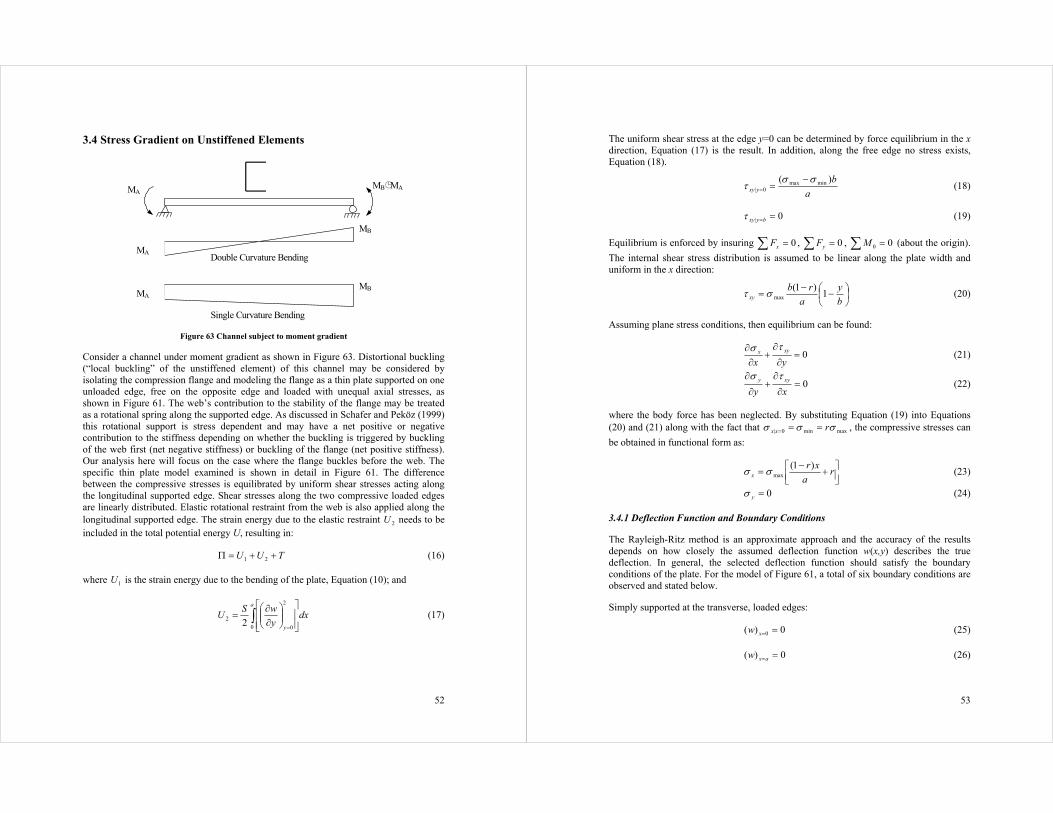
52
3.4 Stress Gradient on Unstiffened Elements
Double Curvature Bending
MB
MB
MB MA MA
MA
MA
Single Curvature Bending
Figure 63 Channel subject to moment gradient
Consider a channel under moment gradient as shown in Figure 63. Distortional buckling (“local buckling” of the unstiffened element) of this channel may be considered by isolating the compression flange and modeling the flange as a thin plate supported on one unloaded edge, free on the opposite edge and loaded with unequal axial stresses, as shown in Figure 61. The web’s contribution to the stability of the flange may be treated as a rotational spring along the supported edge. As discussed in Schafer and Peköz (1999) this rotational support is stress dependent and may have a net positive or negative contribution to the stiffness depending on whether the buckling is triggered by buckling of the web first (net negative stiffness) or buckling of the flange (net positive stiffness). Our analysis here will focus on the case where the flange buckles before the web. The specific thin plate model examined is shown in detail in Figure 61. The difference between the compressive stresses is equilibrated by uniform shear stresses acting along the longitudinal supported edge. Shear stresses along the two compressive loaded edges are linearly distributed. Elastic rotational restraint from the web is also applied along the longitudinal supported edge. The strain energy due to the elastic restraint 2U needs to be included in the total potential energy U, resulting in:
TUU ++=Π 21 (16)
where 1U is the strain energy due to the bending of the plate, Equation (10); and
∫
∂∂
==
a
y
dxy
wSU
0
2
0
2 2 (17)
53
The uniform shear stress at the edge y=0 can be determined by force equilibrium in the x direction, Equation (17) is the result. In addition, along the free edge no stress exists, Equation (18).
a
byxy
)( minmax0|
σστ
−== (18)
0| ==byxyτ (19)
Equilibrium is enforced by insuring ∑ = 0xF , ∑ = 0yF , ∑ = 00M (about the origin).
The internal shear stress distribution is assumed to be linear along the plate width and uniform in the x direction:
−
−=
b
y
a
rbxy 1
)1(maxστ (20)
Assuming plane stress conditions, then equilibrium can be found:
0=∂
∂+
∂∂
yxxyx
τσ (21)
0=∂
∂+
∂
∂
xyxyy τσ
(22)
where the body force has been neglected. By substituting Equation (19) into Equations (20) and (21) along with the fact that maxmin0| σσσ rxx === , the compressive stresses can
be obtained in functional form as:
+
−= r
a
xrx
)1(maxσσ (23)
0=yσ (24)
3.4.1 Deflection Function and Boundary Conditions
The Rayleigh-Ritz method is an approximate approach and the accuracy of the results depends on how closely the assumed deflection function w(x,y) describes the true deflection. In general, the selected deflection function should satisfy the boundary conditions of the plate. For the model of Figure 61, a total of six boundary conditions are observed and stated below.
Simply supported at the transverse, loaded edges:
0)( 0 ==xw (25)
0)( ==axw (26)

54
Elastic restraint against rotation along one supported longitudinal edge:
0)( 0 ==yw (27)
002
2
2
2
==
∂∂
=
∂∂
+∂∂
yyy
wS
x
w
y
wD µ (28)
One free longitudinal edge:
02
2
2
2
=
∂∂
+∂∂
=byx
w
y
wD µ (29)
0)2(2
3
3
3
=
∂∂
∂−+
∂∂
=byyx
w
y
wD µ (30)
Due to the complicated boundary conditions, a single trigonometric (sin or cos) term is not appropriate to approximate the real deflection in either direction. However, the linearity of differential equations (27) to (29) imply that the deflection function ),( yxw
can be formed as ∑=
N
iii xByA
1
)()( , where iA is a function of y alone and iB is a function
of x alone. If, for every i, Ai(y)Bi(x) is compatible with all the boundary conditions, then the linear summation of each term )()( xByA ii will satisfy the boundary conditions. In
this paper, three different approximate deflection functions are proposed and examined.
3.4.2 Deflection Function 1
The first deflection function considered, Equation (32), is motivated by the work of Lundquist and Stowell (1942) who explored the buckling of unstiffened element subject to uniform compressive stresses. Lundquist and Stowell employed a trigonometric term in the longitudinal direction and a polynomial term in the transverse direction to establish the deflection function, as below:
+
+
+
+=
a
x
b
ya
b
ya
b
ya
b
yB
b
yAw
πsin
2
3
3
2
4
1
5
(31)
where A and B are arbitrary deflection amplitudes and 963.41 −=a , 852.92 =a , and
778.93 −=a . The deflection curve across the width of the plate is taken as the sum of a
straight line and a cantilever-deflection curve. The values of 1a , 2a and 3a were
determined by taking the proportion of two deflection curves that gave the lowest buckling stress for a fixed-edge flange with µ =0.3.
55
For the unstiffened element under a stress gradient, the single trigonometric term in the loading direction is no longer appropriate. We therefore use a summation of trigonometric terms in the longitudinal direction and polynomial terms in the transverse direction for the deflection function, Equation (32), where the values of 1a , 2a and 3a
are same as Equation (31).
+
+
+
+= ∑
= a
xi
b
ya
b
ya
b
ya
b
yB
b
yAw
N
i
πsin
1
2
3
3
2
4
1
5
(32)
The arbitrary amplitudes A and B are actually related to each other; the relationship can be obtained by substituting Equation (30) into boundary condition (27), resulting in
ADa
SbB
32= (33)
Therefore, the deflection function, Equation (32), may be simplified as:
+
+
+
+= ∑
= a
xi
b
ya
b
ya
b
ya
b
y
Da
Sb
b
yww
N
ii
πsin
21
2
3
3
2
4
1
5
3
(34)
The equilibrium equations can be constructed by substituting the deflection function into the total potential energy expression Equations (15) and taking the derivative of the function as Equation (12). The buckling stress σmax is the minimum eigenvalue of the resulting matrix of equilibrium expressions. The size of matrix is .NN ×
It should be noted that deflection function 1 is not compatible with boundary the conditions, Equations (28) and (29). However, it was found to give reasonable results in the research done by Lundquist and Stowell (1942) and was thus considered here.
3.4.3 Deflection Function 2
Unlike deflection function 1 which is based on a physical representation of the expected shape, deflection function 2 is a more general combination of polynomials and trigonometric functions. A fourth order polynomial is assumed for the transverse deflection and a sin function for the longitudinal deflection as given in Equation (35).
( )
+++= ∑
= a
xiycycycycww
N
iiiiii
πsin
1
44
33
221 (35)
The deflection function must satisfy all the boundary conditions. Therefore, the parameters 1ic , 2ic , 3ic , 4ic are determined by substituting Equation 35 into the
boundary conditions of Equations (24) to (29), resulting in:
11 =ic (36)

56
D
Sci 22 = (37)
−+
−×
−−−−−+=
22
12
)2()2(2
2
222
1
22
422
32
13212
22
3212
22
32
12
222
32
12
22
3
a
bi
Dk
Sb
a
bi
Dkk
S
Dkkka
bSi
kkka
i
Dkka
Sbi
kka
bici
πµπµ
πµπµπµπµ (38)
Dkk
S
Dkka
bSi
kka
i
Dkka
Sbi
kka
bici
31322
22
322
22
312
222
312
22
4 )2()2(2
−−−−−+=πµπµπµπµ (39)
Ni K,2,1= where
2
322
1 6a
bibk
πµ−= (40)
2
222
2
3)2(6
a
bik
πµ−−= (41)
22
322
212
422
1
2
3
4)2(
2412
ka
bi
k
b
ka
bi
k
bk
πµπµ −+−−= (42)
The equilibrium equations can be constructed by the same method as described for deflection function 1, the buckling stress (σmax)cr is the minimum eigenvalue of the resulting NN × matrix of equilibrium expressions.
3.4.4 Deflection Function 3
As an extension of the second deflection function a third deflection function using a 5th order polynomial in the transverse direction was also considered:
( ) ( )[ ]∑=
++++++=
N
iiiiiiiiii a
xiyqyqyqwypypypypww
1
53
42
312
44
33
2211 sin
π (43)
where 1iw , 2iw are arbitrary deflection amplitudes. The parameters p and q were
determined by the boundary conditions.
11 =ip (44)
D
Spi 22 = (45)
57
12
1422
2
222
112
22
3 22 ka
Mbi
a
bi
Dk
S
ka
bipi
πµπµπµ +
−+= (46)
14 Mpi = (47)
1
22
12
2422
1
3
12
522
1
1220
k
Mb
ka
Mbi
k
b
ka
biqi −+−=
πµπµ (48)
22 Mqi = (49)
13 =iq (50)
where
2
322
1 6a
bibk
πµ−= (51)
2
222
2
3)2(6
a
bik
πµ−−= (52)
22
322
1
22
422
3
124
4)2(
112
kb
a
biv
kb
a
bik
−−−
−=
ππµ (53)
3131
222
312
22
32
22
322
22
1 2)2()2(
kDk
S
Dkk
Sbi
kka
bi
Dkk
bSi
kka
iM +−−−+−=
πµπµπµπµ (54)
31
3
312
522
32
2
322
422
2
20605)2(
kk
b
kka
bi
kk
b
kka
biM +−−−=
πµπµ (55)
The size of the resulting matrix of equilibrium expressions is NN 22 × .
3.4.5 Verification of Three Deflection Functions
Finite element analysis using ABAQUS 6.3 was employed to examine the results of the previous Rayleigh-Ritz solutions. The S4R5 shell element was used for the thin plate with E=29500 ksi and µ=0.3. The element size is 0.1 in. x 0.1 in. The plate is simply supported along three edges, and free along one unloaded edge. The uneven load is equilibrated by shear forces acting along one simply supported edge, similar to Figure 61.
Table 13 provides the buckling stresses calculated by ABAQUS, (σmax)cr (FEM), and the ratio of the Rayleigh-Ritz solutions to the ABAQUS solution. Figure 64 shows the buckled shape for the case with r=0, a=10 in., b=3 in., t=0.0333 in., and S=0 kips-in/in. In general, all three deflection functions give good agreement with the finite element

58
results. Deflection functions 2 and 3 have closer results to the FEM, with average error less than 1%. Deflection function 1 provides systematically higher buckling stress than the FEM results and the other two functions, and the error grows when the stress gradient effect is large or S is large. Since deflection function 2 provides both accuracy and reasonable computational efficiency, it is selected for further analyses. According to a convergence study of deflection function 2, the number of terms to be kept in the expansions (and thus the size of the NxN matrix to be solved,) is selected via the following:
a/b<=10, N=20;
a/b>10 and a/b<=20, N=40;
a/b>20 and a/b<=40, N=60;
a/b>40 and a/b<=60, N=80.
(a) ABAQUS result (b) Rayleigh-Ritz solution
Figure 64 Comparison of buckling shapes of unstiffened element for stress gradient factor r=0
59
Table 13 Results of numerical models with different deflection functions
r a
(in.) b
(in.) T
(in.)
S (kip-in/in)
cr)( maxσ (FEM)
(ksi) DF2/FEM DF2/FEM DF2/FEM
1 10 2.5 0.04 0 3.3277 1.0011 0.9990 0.9979 0.9 10 2.5 0.04 0 3.4976 1.0011 0.9989 0.9979 0.7 10 2.5 0.04 0 3.8523 1.0015 0.9988 0.9977 0.5 10 2.5 0.04 0 4.2131 1.0023 0.9985 0.9973 0.3 10 2.5 0.04 0 4.5697 1.0035 0.9981 0.9968 0.1 10 2.5 0.04 0 4.9198 1.0050 0.9976 0.9962 0 10 2.5 0.04 0 5.0930 1.0058 0.9973 0.9959
-0.1 10 2.5 0.04 0 5.2654 1.0066 0.9971 0.9957 -0.3 10 2.5 0.04 0 5.6091 1.0085 0.9968 0.9951 -0.5 10 2.5 0.04 0 5.9528 1.0107 0.9965 0.9947 -0.7 10 2.5 0.04 0 6.2979 1.0132 0.9963 0.9943 -0.9 10 2.5 0.04 0 6.6450 1.0160 0.9963 0.9940
Case 1
-1 10 2.5 0.04 0 6.8194 1.0196 0.9964 0.9936 1 10 2 0.05 0 7.7316 1.0034 1.0019 1.0009
0.9 10 2 0.05 0 8.1205 1.0035 1.0019 1.0009 0.7 10 2 0.05 0 8.8898 1.0038 1.0016 1.0006 0.5 10 2 0.05 0 9.6180 1.0044 1.0011 1.0000 0.3 10 2 0.05 0 10.3050 1.0052 1.0006 0.9993 0.1 10 2 0.05 0 10.9660 1.0060 0.9999 0.9985 0 10 2 0.05 0 11.2900 1.0065 0.9996 0.9982
-0.1 10 2 0.05 0 11.6120 1.0069 0.9992 0.9978 -0.3 10 2 0.05 0 12.2490 1.0081 0.9987 0.9971 -0.5 10 2 0.05 0 12.8840 1.0093 0.9982 0.9964 -0.7 10 2 0.05 0 13.5170 1.0108 0.9978 0.9959 -0.9 10 2 0.05 0 14.1520 1.0125 0.9974 0.9953
Case 2
-1 10 2 0.05 0 14.4710 1.0133 0.9972 0.9950 1 10 3 0.0333 0 1.6963 1.0004 0.9979 0.9968
0.9 10 3 0.0333 0 1.7836 1.0005 0.9978 0.9967 0.7 10 3 0.0333 0 1.9715 1.0009 0.9978 0.9966 0.5 10 3 0.0333 0 2.1721 1.0019 0.9977 0.9965 0.3 10 3 0.0333 0 2.3793 1.0035 0.9974 0.9962 0.1 10 3 0.0333 0 2.5884 1.0056 0.9972 0.9958 0 10 3 0.0333 0 2.6931 1.0068 0.9971 0.9957
-0.1 10 3 0.0333 0 2.7979 1.0081 0.9970 0.9955 -0.3 10 3 0.0333 0 3.0078 1.0110 0.9969 0.9952 -0.5 10 3 0.0333 0 3.2185 1.0143 0.9970 0.9951 -0.7 10 3 0.0333 0 3.4307 1.0181 0.9974 0.9952 -0.9 10 3 0.0333 0 3.6446 1.0224 0.9979 0.9954
Case 3
-1 10 3 0.0333 0 3.7522 0.9931 0.9983 0.9955 1 10 3 0.0333 inf 4.2469 0.9981 0.9979 0.9975
0.9 10 3 0.0333 Inf 4.4542 0.9991 0.9978 0.9974 0.7 10 3 0.0333 Inf 4.8233 1.0073 0.9969 0.9964 0.5 10 3 0.0333 Inf 5.1333 1.0205 0.9956 0.9951 0.3 10 3 0.0333 Inf 5.4055 1.0363 0.9944 0.9938 0.1 10 3 0.0333 Inf 5.6546 1.0540 0.9933 0.9927 0 10 3 0.0333 Inf 5.7731 1.0636 0.9929 0.9922
-0.1 10 3 0.0333 Inf 5.8887 1.0735 0.9926 0.9918 -0.3 10 3 0.0333 Inf 6.1131 1.0947 0.9920 0.9911 -0.5 10 3 0.0333 Inf 6.3309 1.1176 0.9917 0.9907 -0.7 10 3 0.0333 Inf 6.5442 1.1421 0.9917 0.9905 -0.9 10 3 0.0333 Inf 6.7545 1.1684 0.9918 0.9904
Case 4
-1 10 3 0.0333 inf 6.8587 1.1822 0.9920 0.9905 Mean 1.0237 0.9971 0.9958
Standard deviation 0.0427 0.0026 0.0026

60
Table 14 Numerical results of kmax values of ss-free unstiffened element
r β
-1 -0.8 -0.6 -0.4 -0.2 0 0.2 0.4 0.6 0.8 1
1.0 4.765 4.298 3.841 3.402 2.992 2.621 2.299 2.025 1.796 1.606 1.447
1.2 3.605 3.263 2.930 2.609 2.306 2.029 1.785 1.576 1.399 1.252 1.128
1.4 2.894 2.631 2.375 2.127 1.891 1.673 1.477 1.307 1.163 1.041 0.938
1.6 2.423 2.214 2.009 1.810 1.619 1.440 1.278 1.134 1.010 0.905 0.816
1.8 2.093 1.921 1.752 1.588 1.430 1.279 1.140 1.016 0.906 0.813 0.733
2.0 1.852 1.707 1.565 1.426 1.291 1.162 1.041 0.930 0.832 0.747 0.674
2.5 1.465 1.363 1.264 1.166 1.070 0.976 0.885 0.798 0.718 0.647 0.584
3.0 1.241 1.164 1.088 1.013 0.939 0.866 0.794 0.723 0.655 0.592 0.535
3.5 1.096 1.035 0.974 0.914 0.854 0.795 0.735 0.676 0.616 0.559 0.506
4.0 0.996 0.945 0.894 0.844 0.794 0.744 0.694 0.642 0.590 0.538 0.487
4.5 0.922 0.879 0.836 0.793 0.750 0.707 0.663 0.618 0.571 0.523 0.474
5.0 0.866 0.828 0.791 0.753 0.715 0.677 0.639 0.599 0.556 0.512 0.465
5.5 0.822 0.789 0.755 0.722 0.688 0.654 0.619 0.583 0.545 0.503 0.458
6.0 0.786 0.756 0.726 0.696 0.666 0.635 0.603 0.571 0.536 0.497 0.453
6.5 0.757 0.730 0.703 0.675 0.647 0.619 0.590 0.560 0.528 0.491 0.449
7.0 0.733 0.708 0.683 0.657 0.632 0.606 0.579 0.551 0.521 0.487 0.446
7.5 0.712 0.689 0.665 0.642 0.618 0.594 0.569 0.543 0.515 0.483 0.443
8.0 0.694 0.672 0.651 0.629 0.607 0.584 0.561 0.537 0.510 0.480 0.441
8.5 0.678 0.658 0.638 0.617 0.597 0.576 0.554 0.531 0.506 0.477 0.439
9.0 0.664 0.645 0.627 0.607 0.588 0.568 0.547 0.525 0.502 0.474 0.438
9.5 0.652 0.634 0.617 0.598 0.580 0.561 0.541 0.521 0.498 0.472 0.436
10.0 0.641 0.624 0.608 0.590 0.573 0.555 0.536 0.516 0.495 0.470 0.435
11.0 0.623 0.607 0.592 0.577 0.561 0.544 0.527 0.509 0.489 0.467 0.434
12.0 0.607 0.593 0.579 0.565 0.551 0.535 0.520 0.503 0.485 0.464 0.432
13.0 0.594 0.582 0.569 0.556 0.542 0.528 0.513 0.498 0.481 0.461 0.431
14.0 0.583 0.572 0.560 0.547 0.535 0.522 0.508 0.494 0.478 0.459 0.431
15.0 0.574 0.563 0.552 0.540 0.528 0.516 0.503 0.490 0.475 0.457 0.430
16.0 0.566 0.555 0.545 0.534 0.523 0.511 0.499 0.486 0.472 0.456 0.429
17.0 0.558 0.549 0.539 0.528 0.518 0.507 0.496 0.483 0.470 0.454 0.429
18.0 0.552 0.543 0.533 0.524 0.514 0.503 0.492 0.481 0.468 0.453 0.429
19.0 0.546 0.537 0.528 0.519 0.510 0.500 0.489 0.478 0.466 0.452 0.428
20.0 0.541 0.533 0.524 0.515 0.506 0.497 0.487 0.476 0.464 0.451 0.428
21.0 0.536 0.528 0.520 0.512 0.503 0.494 0.484 0.474 0.463 0.450 0.428
22.0 0.532 0.524 0.516 0.508 0.500 0.491 0.482 0.472 0.461 0.449 0.428
23.0 0.528 0.521 0.513 0.505 0.497 0.489 0.480 0.471 0.460 0.448 0.427
24.0 0.524 0.517 0.510 0.503 0.495 0.487 0.478 0.469 0.459 0.447 0.427
25.0 0.521 0.514 0.507 0.500 0.493 0.485 0.477 0.468 0.458 0.446 0.427
26.0 0.518 0.511 0.505 0.498 0.490 0.483 0.475 0.466 0.457 0.446 0.427
27.0 0.515 0.509 0.502 0.496 0.489 0.481 0.474 0.465 0.456 0.445 0.427
28.0 0.513 0.506 0.500 0.493 0.487 0.480 0.472 0.464 0.455 0.445 0.427
29.0 0.510 0.504 0.498 0.492 0.485 0.478 0.471 0.463 0.454 0.444 0.427
30.0 0.508 0.502 0.496 0.490 0.483 0.477 0.470 0.462 0.454 0.444 0.427
61
Table 15 Numerical results of kmax values for fix-free unstiffened element
r β
-1 -0.8 -0.6 -0.4 -0.2 0 0.2 0.4 0.6 0.8 1
1.0 5.073 4.626 4.187 3.760 3.351 2.971 2.628 2.327 2.071 1.854 1.672
1.2 4.024 3.702 3.386 3.077 2.776 2.490 2.223 1.982 1.770 1.587 1.432
1.4 3.404 3.161 2.922 2.687 2.457 2.233 2.017 1.815 1.630 1.466 1.323
1.6 3.012 2.820 2.632 2.448 2.268 2.089 1.914 1.742 1.578 1.425 1.288
1.8 2.749 2.594 2.442 2.294 2.148 2.005 1.863 1.720 1.577 1.434 1.299
2.0 2.566 2.437 2.311 2.187 2.067 1.950 1.834 1.719 1.601 1.476 1.343
2.5 2.291 2.201 2.112 2.025 1.939 1.855 1.772 1.689 1.605 1.514 1.396
3.0 2.139 2.067 1.996 1.925 1.854 1.781 1.705 1.623 1.532 1.424 1.299
3.5 2.037 1.976 1.915 1.853 1.790 1.725 1.656 1.583 1.503 1.410 1.293
4.0 1.961 1.907 1.853 1.797 1.741 1.682 1.622 1.558 1.492 1.421 1.343
4.5 1.901 1.853 1.804 1.753 1.702 1.649 1.594 1.537 1.474 1.402 1.299
5.0 1.853 1.809 1.763 1.718 1.670 1.622 1.571 1.518 1.459 1.390 1.287
5.5 1.813 1.772 1.730 1.688 1.644 1.599 1.552 1.503 1.449 1.387 1.304
6.0 1.779 1.741 1.702 1.662 1.622 1.580 1.536 1.490 1.439 1.382 1.299
6.5 1.749 1.714 1.678 1.641 1.603 1.563 1.522 1.478 1.431 1.375 1.287
7.0 1.724 1.691 1.657 1.622 1.586 1.549 1.510 1.469 1.424 1.371 1.293
7.5 1.702 1.670 1.638 1.605 1.571 1.536 1.499 1.460 1.417 1.368 1.299
8.0 1.682 1.652 1.622 1.591 1.558 1.525 1.490 1.452 1.412 1.364 1.288
8.5 1.665 1.636 1.607 1.577 1.547 1.515 1.481 1.445 1.406 1.361 1.289
9.0 1.649 1.622 1.594 1.566 1.536 1.506 1.473 1.439 1.402 1.358 1.299
9.5 1.635 1.609 1.582 1.555 1.527 1.497 1.466 1.434 1.398 1.356 1.289
10.0 1.622 1.597 1.571 1.545 1.518 1.490 1.460 1.428 1.394 1.353 1.287
11.0 1.599 1.576 1.552 1.528 1.503 1.476 1.449 1.419 1.387 1.349 1.290
12.0 1.580 1.558 1.536 1.513 1.490 1.465 1.439 1.412 1.381 1.346 1.290
13.0 1.563 1.543 1.522 1.501 1.478 1.455 1.431 1.405 1.376 1.342 1.287
14.0 1.549 1.530 1.510 1.490 1.469 1.447 1.424 1.399 1.372 1.340 1.291
15.0 1.536 1.518 1.499 1.480 1.460 1.439 1.417 1.394 1.368 1.337 1.287
16.0 1.525 1.507 1.490 1.471 1.452 1.432 1.412 1.389 1.364 1.335 1.288
17.0 1.515 1.498 1.481 1.464 1.445 1.426 1.406 1.385 1.361 1.333 1.289
18.0 1.506 1.490 1.473 1.457 1.439 1.421 1.402 1.381 1.358 1.332 1.287
19.0 1.497 1.482 1.466 1.450 1.434 1.416 1.398 1.378 1.356 1.330 1.289
20.0 1.490 1.475 1.460 1.445 1.428 1.412 1.394 1.375 1.353 1.328 1.287
21.0 1.483 1.469 1.454 1.439 1.424 1.407 1.390 1.372 1.351 1.327 1.288
22.0 1.476 1.463 1.449 1.434 1.419 1.404 1.387 1.369 1.349 1.326 1.288
23.0 1.471 1.457 1.444 1.430 1.415 1.400 1.384 1.367 1.347 1.325 1.287
24.0 1.465 1.452 1.439 1.426 1.412 1.397 1.381 1.364 1.346 1.324 1.288
25.0 1.460 1.448 1.435 1.422 1.408 1.394 1.378 1.362 1.344 1.323 1.287
26.0 1.455 1.443 1.431 1.418 1.405 1.391 1.376 1.360 1.342 1.322 1.287
27.0 1.451 1.439 1.427 1.415 1.402 1.388 1.374 1.358 1.341 1.321 1.288
28.0 1.447 1.435 1.424 1.412 1.399 1.386 1.372 1.357 1.340 1.320 1.287
29.0 1.443 1.432 1.420 1.409 1.396 1.383 1.370 1.355 1.339 1.319 1.288
30.0 1.439 1.428 1.417 1.406 1.394 1.381 1.368 1.353 1.337 1.319 1.287

62
3.4.6 Results
Two unstiffened elements are investigated here, one where the supported longitudinal edge has no rotational restraint (ss-free) and one where the supported has infinite rotational restraint (fix-free). The plate buckling coefficient kmax for the elements subject to a variety of stress gradients is summarized in Table 14 for the ss-free case and Table 15 for the fix-free case. Figure 65 and Figure 65 give a graphic representation of the stress gradient effect on these two different unstiffened elements. For the ss-free unstiffened plate under uniform compression, the plate buckling coefficient k asymptotes to 0.425. It is shown in Figure 65 that the stress gradient boosts the buckling stress at the maximum loaded edge greatly, especially when the plate aspect ratio (β) is less than 10. Similar results are observed for the fix-free unstiffened element in Figure 66, the buckling coefficient kmax converges to 1.287 (buckling coefficient for uniform compression) gradually.
0 5 10 15 20 25 300
0.5
1
1.5
2
2.5
β
kmax
r = −1 r = −0.8r = −0.6r = −0.4r = −0.2r = 0 r = 0.2 r = 0.4 r = 0.6 r = 0.8 r = 1
Figure 65 kmax vs. plate aspect ratio (β) for ss-free unstiffened element
Figure 67 shows the relation between the plate buckling coefficient kmax and the stress gradient factor r for a ss-free unstiffened element. Figure 67 indicates that the increase in the plate buckling coefficient kmax can be assumed a linear function with r except for approximately square (β =1) plates. For design, we intend to provide simple empirical relations for kmax(r, β, S)
ss
free
ss
free
ss
free
maxσ
maxσ
maxσ
tb
Dkcr 2
2
maxmax )(πσ =
63
0 5 10 15 20 25 301
1.5
2
2.5
3
3.5
4
β
r = −1 r = −0.8 r = −0.6 r = −0.4 r = −0.2 r = 0 r = 0.2 r = 0.4 r = 0.6 r = 0.8 r = 1
kmax
Figure 66 kmax vs. plate aspect ratio (β) for fix-free unstiffened element
Figure 67 kmax vs. stress gradient factor r for ss-free unstiffened element
fix
free
fix
free
fix
free
maxσ
maxσ
maxσ
tb
Dkcr 2
2
maxmax )(πσ =

64
3.5 Discussion
Figure 68 shows a comparison of the three different elements subject to a stress gradient with r=0 (compressive stress only acting on one edge). The y axis is the stress gradient solutions derived here, normalized to k0 which is the solution for elements under uniform stress (no stress gradient, r=1). As shown in Figure 68, the stress gradient has the most influence on the ss-free unstiffened element. The plate buckling coefficient for the stiffened element kmax converges rapidly to approximately 1.1k0 and then more slowly to 1.0 k0. For the ss-free unstiffened element kmax>1.1k0, even for β as large as 30. However, the fix-free unstiffened element is approximate the same as the stiffened element. The moment gradient influence on unstiffened sections can be expected in the area between the curves of ss-free and fix-free unstiffened elements of Figure 68. If we compare to the section in Figure 59, if a moment gradient went from a maximum to an inflection point (M=0, r=0) over a length of 4 in. x 30 = 120 in. (10 ft.) then one would expect a boost in the plate buckling coefficient of as much as 1.1 – if the moment gradient is sharper the boost would be greater. The significant influence on the unstiffened element, particularly in the case where the web provides little restraint, can make the moment gradient a considerable factor when one analyzes the buckling strength. These solutions suggest a reserve that may be relied upon in many loading cases, particularly with regard to unstiffened elements.
Figure 68 Comparison of stiffened and unstiffened elements subject to stress gradient r=0
maxσ
65
4. Conclusions
Experiments on a wide variety of industry standard laterally braced C and Z beams where the compression flange is unrestrained over a distance of 64 in. indicate that distortional buckling is the most likely failure mode. Distortional failures occur even when local buckling is at a lower critical elastic moment than distortional buckling. Previous testing (Phase 1 of this project) demonstrated that if additional rotational restraint can be provided to the compression flange, such as through engagement of a through-fastened deck, the distortional mode can be avoided and a local mode triggered instead. While in nearly all of the sections distortional buckling dominated the failure other limit states are possible, even at unbraced lengths of 64 inches. For example, in one test on an 8 in. deep C beam with a nominal t = 0.097 in. and a 64 in. unbraced length lateral-torsional buckling (LTB) initiated the failure. The thicker specimens have high local and distortional buckling stresses and can thus be controlled by LTB. The thinnest specimens may also be controlled by other limit states, one member was observed to fail in local buckling, and another in a shear + bending failure. While these failure modes were uncommon they serve to demonstrate the variety of behavior that may occur at even modest unbraced lengths.
Comparison of the experimental results with existing and proposed design specifications indicates that the previously employed American Specification (AISI) and Canadian Standard (S136) as well as the newly adopted joint North American Specification (NAS) provide a poor prediction of the strength for members failing in the distortional mode. Errors are, on average, 10 – 15 % unconservative for these design specifications. The Eurocode which provides some measures for distortional buckling is, on average, 5% unconservative. Two methods which include explicit procedures for distortional buckling the Australian/New Zealand (AS/NZS) standard and the Direct Strength Method (recently adopted as Appendix 1 of the NAS) provide far better predictions in distortional failures with conservative errors of, on average, 2% and 1% for the respective methods.
A non-linear finite element model of the testing has been setup and verified by the experimental data. The extended FE analysis has been carried out to a number of cold-formed steel beams which are not included in the two series tests. The results show Direct Strength Method gives reasonable and conservative predictions for both local and distortional buckling strength of beams. The analysis is still undergoing and more geometric sections will be examined.
An analytical method to determine the buckling stress of thin plates subject to a stress gradient is derived and verified by finite element analysis. The results show that under astress gradient, the buckling stress at the maximum loading end is higher than the uniform buckling stress of the same plate. Compared with the stiffened element, the unstiffened element has more influence by the stress gradient and the influence vanishes more slowly when the plate aspect ratio becomes large. It indicates that ignoring the moment gradient effect leads to conservative predictions of the strength of thin-walled beams, particular for the cases where the web provides little restraint to the flange. The authors intend to seek simple empirical expression kmax(r, β, S) for thin plates and further

66
develop the code provisions to account for the moment gradient effect on thin-walled beams.
Using the experiments and the finite element analysis, research is now underway to explore the influence of partial restraint and moment gradient on the bending strength of laterally braced cold-formed steel members and development of code provisions to account for these phenomena.
Acknowledgement
The sponsorship of AISI for both phases of this work, and MBMA for phase 1 and a graduate fellowship is gratefully acknowledged. Donation of materials by Varco-Pruden, Clark Steel and the Dietrich Design Group is also gratefully acknowledged. The assistance of the AISI task group in developing the testing plan is appreciated. Don Johnson, Maury Golovin, Joe Nunnery, Joe Wellinghoff, and Steve Thomas have all been helpful with their ideas and generous with their time. The experiments would not have been possible without the help of Johns Hopkins undergraduates, Liakos Ariston, Brent Bass, Andrew Myers, Sam Phillips, and Tim Ruth, Sam’s work during Phase 1 and Tim’s during Phase 2 has been particularly helpful. Finally, the work has been helpfully aided by the laboratory technician Jack Spangler, and our machinist Jim Kelly.
References
AISI (1996). “Specification for the Design of Cold-Formed Steel Structural Members.
1996”, American Iron and Steel Institute. Washington, D.C. ASTM (2000) “E8-00, Standard test methods for tension testing of metallic material”,
American Society for Testing and Materials. Pennsylvania. Elhouar, S., Murray, T.M. (1985) “Adequacy of Proposed AISI Effective Width
Specification Provisions for Z- and C-Purlin Design.” FSEL/MBMA 85-04, Univ. of Oklahoma.
ABAUQS (2001). ABAQUS Version 6.2., ABAQUS, Inc. Pawtucket, RI.
(www.abaqus.com) NAS (2001). “ North American Specification for the Design of Cold-Formed Steel
Structural Members.”, American Iron and Steel Institute, Washington, D.C. S136 (1994). “Cold-Formed Steel Structural Members” S136-94. Canadian Standards
Association. Ontario, Canada. AS/NZS (1996). AS/NZS 4600: 1996 Cold-Formed Steel Structures. Standards Australia
and the Australian Institute of Steel Construction EN1993 (2002) “European Standard EN1993-1-3. Eurocode 3: Design of steel structure”
European Committee for Standardization. DSM (2003) “Appendix 1 of the North American Specification for the Design of Cold-
formed Steel Structural Members.” American Iron and Steel Institute, Washington, D.C.
67
Hancock, G.J., Rogers, C.A., Schuster, R.M. (1996). “Comparison of the Distortional
Buckling Method for Flexural Members with Tests.” 13th In’l. Spec. Conf. on Cold-Formed Steel Structures, 125-140, St. Louis, MO.
Rogers, C.A., Schuster, R.M. (1995) “Interaction Buckling of Flange, Edge Stiffener and
Web of C-Sections in Bending.” Research Into Cold Formed Steel, Final Report of CSSBI/IRAP Project, Department of Civil Engineering, University of Waterloo, Waterloo, Ontario.
Schafer, B.W. (2002a). “Local, Distortional, and Euler Buckling in Thin-walled
Columns.” J. of Struct. Eng., ASCE, 128(3) 289-299. Schafer, B.W. (2002b). “Design Manual for Direct Strength Method of Cold-Formed
Steel Design.”, AISI, Washington, D.C. (www.ce.jhu.edu/bschafer/direct_strength). Schafer, B.W. (2001). "CUFSM 2.5: Users Manual and Tutorials"
(www.ce.jhu.edu/bschafer/cufsm). Schafer, B.W., Peköz, T. (1999). “Laterally Braced Cold-Formed Steel Flexural
Members with Edge Stiffened Flanges.”, J. of Struct. Eng. ASCE, 125(2) 118-127. Schafer, B.W., Peköz, T. (1998a). “Direct Strength Prediction of Cold-Formed Steel
Members using Numerical Elastic Buckling Solutions.” 14th Int’l. Spec. Conf. on Cold-Formed Steel Structures, St. Louis, Missouri.
Schafer, B.W., Peköz, T. (1998b). “Computational Modeling of Cold-Formed Steel:
Characterizing Geometric Imperfections and Residual Stresses.” Elsevier, Journal of Constructional Steel Research. 47 (3) 193-210.
Yu, C., Schafer, B.W. (2003). “Local buckling Test on Cold-Formed Steel Beams” ASCE
Journal of Structural Engineering. 129 (12) 1596-1606.
Yu, C., Schafer, B.W. (2002). “Local buckling Test on Cold-Formed Steel Beams” 16th
Int’l Spec. Conf. on Cold-Formed Steel Structures, Orlando, Florida Lundquist E., Stowell E. (1942). “Critical Compressive Stress for Outstanding Flanges”. NACA Report No. 734. National Advisory Committee for Aeronautics, Washington, 1942. Libove, C., Ferdman, S., Reusch, J. (1949). “Elastic Buckling of A Simply Supported Plate Under A Compressive Stress That Varies Linearly in the Direction of Loading”. NACA Technical Notet No. 1891. National Advisory Committee for Aeronautics, Washington, 1949. Timoshenko, S.P., Gere, J.M. (1961). “Theory of Elastic Stability”, Second Edition. McGrqw-Hill Book Co., 1961 Lau, S.C.W., Hancock, G.J. (1987). “Distortional Buckling Formulas for Channel Columns” ASCE, Journal of Structural Engineering. 113 (5) 1063-1078. Schafer, B.W., Peköz, T. (1999). “Laterally Braced Cold-Formed Steel Flexural Members with Edge Stiffened Flanges” ASCE, Journal of Structural Engineering. 125 (2) 118-127.

68
Appendix: Summary of Recent Work
By Cheng Yu
A1. Distortional Buckling Tests
Since last report for AISI in February 2004, five more distortional buckling tests, including the tensile tests, on C beans have been completed. So far, all the available geometries of cold-formed steel sections have been tested Among the 24 distortional buckling tests, 7 of them are believed not to fail in distortional buckling mode. The tests show that without the full restraint on the compression flange, the cold-formed steel beam can fail in local and lateral torsional buckling. In average, the full restraint on flange can increase the bending strength by 20%.
The main body of North American Specification NAS 2002, AISI 1996 and CSA S136 are adequate for strength predictions of beams in local buckling failure. Direct Strength Method, Eurocode EN1993 and AS/NZS 4600 provide good agreement with the experimental results for both local and distortional buckling tests.
A2. Finite Element Modeling
The finite element model by ABAQUS uses shell elements for the purlins, decking and tubes; solid elements for the loading beam. The auto Stabilization method in ABAQUS is employed for the nonlinear inelastic analysis. The modified Riks method was originally considered but not used later on because it always has convergence related problems when analysis comes to the peak load region. Figure A1 shows a comparison of these two methods on a Z beam test. The Modified Riks method ends due to error, the auto Stabilization method works well.
Figure A1 Comparison of nonlinear algorithms
69
Geometric imperfection and material nonlinearity are considered in the finite element model. And it has been used to simulate the completed tests; the results validate the FEA model. Then the FE analysis was extended to a number of beams which are not performed in the lab. Up to now, total 45 local buckling and 45 distortional buckling tests have been analyzed by the FE model. The results as shown in Figure A2 indicates that the Direct Strength Method works well for both failure mode.
Figure A2 FEA results vs. DSM predications
A3. Stress Gradient Effect on the Thin Plate
The research of the stress gradient (in the loading direction) effect on the thin plate is the first step towards a successful understanding of the moment gradient effect on the cold-formed beams. The result will help to study the stress gradient effect on the Winter’s curve which is essential to the Effective Width Concept and the strength curve based design methods like the Direct Strength Method and AS/NZS specification.
A3.1 Elastic Buckling
The elastic buckling of think plate under stress gradient has already been well studied. The analytical method used to calculate the buckling stresses and the results are detailed in the report. Beyond the content in the report, two deflection functions (Equation A1 and A2) for the stiffened element are newly derived. Unlike Libove’s work (Libove 1949), the new deflection functions can calculate the buckling of stiffened element with elastic restraint on the two longitudinal edges as shown in Figure A3.
[ ]
−+−= ∑
= a
xibyyBbyyAw
N
iii
πsin)()(
1
2 (A1)
+−= ∑
= a
xi
b
yBbyyAw
N
iii
ππsinsin)(
1
(A2)

70
o
Y
min σ max σ
τ
a
b simply supported and elastically restrained
X
τ
τ τ
Figure A3 Analytical model of stiffened element with elastic restraint on edges
The two new deflection functions and the deflection function used by Libov 1949 are being verified by finite element model of ABAQUS. The examination work has not been finished yet, but the up to date result (summarized in Table A1) is promising. It is shown that the deflection 2 gives the best result.
Table A1 Comparison of three analytical model with the FE results
r
a (in.)
b (in.)
t (in.)
S(kip-in/in)
cr)( maxσ (FEM)
(ksi) DF1/FEM DF2/FEM Libove/FEM
1 10 2.5 0.04 0 27.469 71.66% 99.39% 99.38%
0.9 10 2.5 0.04 0 28.480 72.63% 99.66% 99.82%
0.7 10 2.5 0.04 0 29.706 76.56% 100.04% 100.82%
0.5 10 2.5 0.04 0 30.725 80.65% 100.13% 101.74%
0.3 10 2.5 0.04 0 31.668 84.42% 100.13% 102.72%
0.1 10 2.5 0.04 0 32.567 87.84% 100.09% 103.79%
0 10 2.5 0.04 0 33.006 89.44% 100.05% 104.34%
-0.1 10 2.5 0.04 0 33.438 90.99% 100.01% 104.94%
-0.3 10 2.5 0.04 0 34.288 93.96% 99.91% 106.19%
-0.5 10 2.5 0.04 0 35.124 96.83% 99.80% 107.56%
-0.7 10 2.5 0.04 0 35.948 99.63% 99.69% 109.05%
-0.9 10 2.5 0.04 0 36.764 97.41% 99.56% 110.68%
Case 1
-1 10 2.5 0.04 0 37.170 96.35% 99.50% NA 1 12 3 0.05 0 29.657 72.01% 99.89% 99.89%
0.9 12 3 0.05 0 31.074 72.24% 99.11% 99.26% 0.7 12 3 0.05 0 32.046 76.99% 100.62% 101.42% 0.5 12 3 0.05 0 33.125 81.16% 100.78% 102.40% 0.3 12 3 0.05 0 34.121 85.02% 100.84% 103.44% 0.1 12 3 0.05 0 35.071 88.51% 100.85% 104.56% 0 12 3 0.05 0 35.532 90.15% 100.84% 105.16%
-0.1 12 3 0.05 0 35.987 91.75% 100.83% 105.79% -0.3 12 3 0.05 0 36.881 94.79% 100.79% 107.13% -0.5 12 3 0.05 0 37.759 97.73% 100.74% 108.58% -0.7 12 3 0.05 0 38.623 100.62% 100.67% 110.14% -0.9 12 3 0.05 0 39.478 98.43% 100.61% 111.84%
Case 2
-1 12 3 0.05 0 39.902 97.39% 100.57% NA Mean 87.89% 100.20% 104.61%
Standard deviation 9.6% 0.5% 3.7%
71
A3.2 Ultimate Strength
Nonlinear inelastic analysis by ABAQUS is used to study the ultimate strength/postbuckling behavior of thin plate under stress gradient in the longitudinal direction. The main work is to verify the Winter’s curve (Equation A3) for the stress gradient cases.
122.0
1 ≤
−= λ
λρ (A3)
where E
f
t
w
k
=
052.1λ
k= plate buckling coefficient t= thickness of compression element E= modulus of elasticity f= maximum compressive edge stress in the element without considering the
safety factor.
The finite element model uses shell element S4R5 for the plate. The shape of initial geometric imperfection is assumed to be the first buckling mode. The maximum initial deflection is scaled to 50% CDF of the local buckling shape, d/t=0.34 (Schafer 1998). The material stress vs. strain curves are determined from the real tensile tests in the buckling tests just completed. Five different yield strength levels are selected: 33 ksi, 44 ksi, 56.1 ksi, 62.2 ksi, 73.4 ksi. The Modified Riks method in ABAQUS is employed.
0.0
0.2
0.4
0.6
0.8
1.0
1.2
0.00 1.00 2.00 3.00 4.00 5.00λ
Winter curve
ABAQUS r=1
ABAQUS r=0
Figure A4 ABAQUS results vs. Winter’s curve
Figure A4 shows the comparison of ABAQUS results with the Winter’s curve. The data is summarized in Table A2 and Table A3. “ABAQUS r=1” is the stiffened (simply
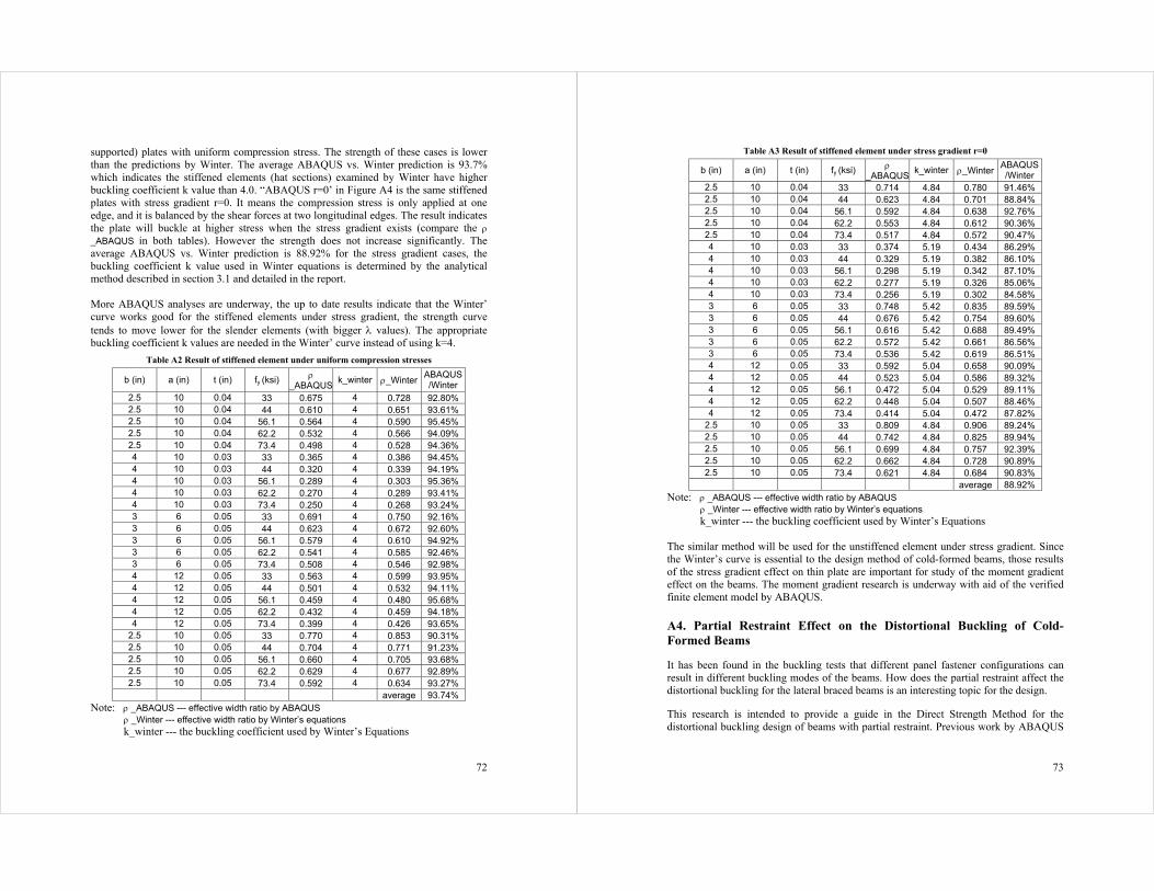
72
supported) plates with uniform compression stress. The strength of these cases is lower than the predictions by Winter. The average ABAQUS vs. Winter prediction is 93.7% which indicates the stiffened elements (hat sections) examined by Winter have higher buckling coefficient k value than 4.0. “ABAQUS r=0’ in Figure A4 is the same stiffened plates with stress gradient r=0. It means the compression stress is only applied at one edge, and it is balanced by the shear forces at two longitudinal edges. The result indicates the plate will buckle at higher stress when the stress gradient exists (compare the ρ _ABAQUS in both tables). However the strength does not increase significantly. The average ABAQUS vs. Winter prediction is 88.92% for the stress gradient cases, the buckling coefficient k value used in Winter equations is determined by the analytical method described in section 3.1 and detailed in the report. More ABAQUS analyses are underway, the up to date results indicate that the Winter’ curve works good for the stiffened elements under stress gradient, the strength curve tends to move lower for the slender elements (with bigger λ values). The appropriate buckling coefficient k values are needed in the Winter’ curve instead of using k=4.
Table A2 Result of stiffened element under uniform compression stresses
b (in) a (in) t (in) fy (ksi) ρ _ABAQUS
k_winter ρ_WinterABAQUS/Winter
2.5 10 0.04 33 0.675 4 0.728 92.80% 2.5 10 0.04 44 0.610 4 0.651 93.61% 2.5 10 0.04 56.1 0.564 4 0.590 95.45% 2.5 10 0.04 62.2 0.532 4 0.566 94.09% 2.5 10 0.04 73.4 0.498 4 0.528 94.36% 4 10 0.03 33 0.365 4 0.386 94.45% 4 10 0.03 44 0.320 4 0.339 94.19% 4 10 0.03 56.1 0.289 4 0.303 95.36% 4 10 0.03 62.2 0.270 4 0.289 93.41% 4 10 0.03 73.4 0.250 4 0.268 93.24% 3 6 0.05 33 0.691 4 0.750 92.16% 3 6 0.05 44 0.623 4 0.672 92.60% 3 6 0.05 56.1 0.579 4 0.610 94.92% 3 6 0.05 62.2 0.541 4 0.585 92.46% 3 6 0.05 73.4 0.508 4 0.546 92.98% 4 12 0.05 33 0.563 4 0.599 93.95% 4 12 0.05 44 0.501 4 0.532 94.11% 4 12 0.05 56.1 0.459 4 0.480 95.68% 4 12 0.05 62.2 0.432 4 0.459 94.18% 4 12 0.05 73.4 0.399 4 0.426 93.65%
2.5 10 0.05 33 0.770 4 0.853 90.31% 2.5 10 0.05 44 0.704 4 0.771 91.23% 2.5 10 0.05 56.1 0.660 4 0.705 93.68% 2.5 10 0.05 62.2 0.629 4 0.677 92.89% 2.5 10 0.05 73.4 0.592 4 0.634 93.27%
average 93.74% Note: ρ _ABAQUS --- effective width ratio by ABAQUS ρ _Winter --- effective width ratio by Winter’s equations k_winter --- the buckling coefficient used by Winter’s Equations
73
Table A3 Result of stiffened element under stress gradient r=0
b (in) a (in) t (in) fy (ksi) ρ _ABAQUS
k_winter ρ_Winter ABAQUS /Winter
2.5 10 0.04 33 0.714 4.84 0.780 91.46% 2.5 10 0.04 44 0.623 4.84 0.701 88.84% 2.5 10 0.04 56.1 0.592 4.84 0.638 92.76% 2.5 10 0.04 62.2 0.553 4.84 0.612 90.36% 2.5 10 0.04 73.4 0.517 4.84 0.572 90.47% 4 10 0.03 33 0.374 5.19 0.434 86.29% 4 10 0.03 44 0.329 5.19 0.382 86.10% 4 10 0.03 56.1 0.298 5.19 0.342 87.10% 4 10 0.03 62.2 0.277 5.19 0.326 85.06% 4 10 0.03 73.4 0.256 5.19 0.302 84.58% 3 6 0.05 33 0.748 5.42 0.835 89.59% 3 6 0.05 44 0.676 5.42 0.754 89.60% 3 6 0.05 56.1 0.616 5.42 0.688 89.49% 3 6 0.05 62.2 0.572 5.42 0.661 86.56% 3 6 0.05 73.4 0.536 5.42 0.619 86.51% 4 12 0.05 33 0.592 5.04 0.658 90.09% 4 12 0.05 44 0.523 5.04 0.586 89.32% 4 12 0.05 56.1 0.472 5.04 0.529 89.11% 4 12 0.05 62.2 0.448 5.04 0.507 88.46% 4 12 0.05 73.4 0.414 5.04 0.472 87.82%
2.5 10 0.05 33 0.809 4.84 0.906 89.24% 2.5 10 0.05 44 0.742 4.84 0.825 89.94% 2.5 10 0.05 56.1 0.699 4.84 0.757 92.39% 2.5 10 0.05 62.2 0.662 4.84 0.728 90.89% 2.5 10 0.05 73.4 0.621 4.84 0.684 90.83%
average 88.92% Note: ρ _ABAQUS --- effective width ratio by ABAQUS ρ _Winter --- effective width ratio by Winter’s equations k_winter --- the buckling coefficient used by Winter’s Equations The similar method will be used for the unstiffened element under stress gradient. Since the Winter’s curve is essential to the design method of cold-formed beams, those results of the stress gradient effect on thin plate are important for study of the moment gradient effect on the beams. The moment gradient research is underway with aid of the verified finite element model by ABAQUS.
A4. Partial Restraint Effect on the Distortional Buckling of Cold-Formed Beams
It has been found in the buckling tests that different panel fastener configurations can result in different buckling modes of the beams. How does the partial restraint affect the distortional buckling for the lateral braced beams is an interesting topic for the design.
This research is intended to provide a guide in the Direct Strength Method for the distortional buckling design of beams with partial restraint. Previous work by ABAQUS

74
and CUFSM indicates that the panel fastener in full testing setup can be modeled as a rotation spring in finite strip analysis (CUFSM), Figure A5, which provides a simple way to calculate the elastic buckling moment of beams with restraints.
Figure A5 Finite strip analysis of partial restraint section
With the aid of the nonlinear FE model by ABAQUS, research is underway to examine the ultimate strength of lateral braced beams with different fastened panel configurations.
A5. The Outline of the Doctoral Thesis
Chapter 1 Introduction 1.1 Cold-Formed Steel Structural Members 1.2 Design Methods for Cold-Formed Steel Structural Members
1.2.1 Design Specifications for Cold-Formed Steel Structural Members 1.2.2 The Effective Width Concept 1.2.3 New Design Method – Direct Strength Method
1.3 Motivation and Objectives 1.4 Outline of Thesis
Chapter 2 Local Buckling Tests on Cold-Formed Steel Beams 2.1 Introduction 2.2 Local Buckling Tests
2.2.1 Specimen Selection 2.2.2 Specimen Dimensions 2.2.3 Testing Details 2.2.4 Panel-to-Purlin Fastener Configuration
2.3 Experimental Results 31 2.4 Comparison with Design Methods
2.4.1 Test-to-Predicted Ratio 2.4.2 The Web Effective Width
2.5 Conclusions
Chapter 3 Distortional Buckling Tests on Cold-Formed Steel Beams 3.1 Introduction
75
3.2 Distortional Buckling Tests 3.2.1 Specimen Selection and Dimensions 3.2.2 Testing Setup 3.2.3 Panel-to-Purlin Fastener Configuration
3.3 Experimental Results 3.4 Examination of Several Tests of Note
3.4.1 Test Failed in Lateral-Torsional Buckling Mode: Re-Test of D8C097 3.4.2 Test Failed by Material Yielding: D3.62C054-3E4W 3.4.3 Tests Failed in Local Buckling Mode 3.4.4 Tests Failed in Unexpected Mode
3.5 Comparison with Local Buckling Tests 3.6 Comparison with Design Methods
3.7 Conclusions
Chapter 4 Tensile Tests 4.1 Introduction 4.2 Testing Setup 4.3 Experimental Results Chapter 5 Finite Element Modeling of Cold-Formed Beams 5.1 Introduction 5.2 Elastic Buckling Solution Methods
5.2.1 Finite Element Method 5.2.2 Finite Strip Method
5.3 Ultimate Strength Solution Method/Postbuckling Strength Analysis 5.3.1 Modified Riks Method 5.3.2 STABILIZ Method in ABAQUS
5.4 Finite Element Modeling 5.4.1 Shell Element 5.4.2 Modeling Details and Loading/Boundary Conditions 5.4.3 Geometric Imperfection 5.4.4 Material Modeling 5.4.5 Residual Stress
5.5 Finite Element Analysis 5.5.2 Elastic Buckling Results 5.5.3 Ultimate Strengths/Postbuckling Results
5.6 Conclusions
Chapter 6 Applications of the Finite Element Modeling 6.1 Introduction
6.2 Extended Finite Element Analysis on Cold-Formed Steel Beams 6.2.1 Selection of Specimens 6.2.2 Comparison with Direct Strength Method
6.3 Moment Gradient Effect on Cold-Formed Steel Beams 6.3.1 FE Modeling 6.3.2 Results

76
6.4 Partial Restraint Effect on Lateral Braced Beams 6.4.1 FE Modeling 6.4.2 Results 6.5 Conclusions
Chapter 7 Stress Gradient Effect on Thin Plates 7.1 Introduction 7.1 Analytic Solution: Energy Method 7.2 Stress Gradient on Elastic Buckling of Stiffened Elements
7.2.1 Deflection function and boundary conditions 7.2.2 Early work and Recalculation 1 7.2.3 Deflection Function 1 7.2.4 Deflection Function 2 7.2.5 Verification by Finite Element Model 7.2.6 Results
7.3 Stress Gradient on Elastic Buckling of Unstiffened Elements 7.3.1 Deflection function and boundary conditions 7.3.2 Deflection function 1 7.3.3 Deflection Function 2 7.3.4 Deflection Function 3 7.3.5 Verification by Finite Element Model 7.3.6 Results 7.3.7 Discussion
7.4 Ultimate Strength of Stiffened Elements under Stress Gradient 7.4.1 Finite Element Model 7.4.2 Comparison with Winter Equations
7.5 Ultimate Strength of Unstiffened Element under Stress Gradient 7.5.1 Finite Element Model 7.5.2 Comparison with Winter Equations
7.6 Conclusions
Chapter 8 Design of Cold-Formed Steel Beams in Distortional Buckling Failures 8.1 Introduction 8.1 Distortional Buckling of Beams under Moment Gradient 8.2 Distortional Buckling of Beams with Partial Restraint 8.3 Conclusions
Chapter 9 Conclusions and Recommendations 9.1 Summary
9.2 Recommendations for Future Research
Reference Appendix A --- Data Sheets for the Local buckling Test of Cold-Formed Steel Beams Appendix B --- Data Sheets for the Distortional buckling Test of Cold-Formed Steel Beams
77
A6. Reference
Yu, C; Schafer, B.W (2004). “Report to The American Iron and Steel Institute (AISI)”, August 2004
ABAUQS (2001). ABAQUS Version 6.2., ABAQUS, Inc. Pawtucket, RI.
(www.abaqus.com) Schafer, B.W. (2001). "CUFSM 2.5: Users Manual and Tutorials"
(www.ce.jhu.edu/bschafer/cufsm). Schafer, B.W., Peköz, T. (1998). “Computational Modeling of Cold-Formed Steel:
Characterizing Geometric Imperfections and Residual Stresses.” Elsevier, Journal of Constructional Steel Research. 47 (3) 193-210.
Libove, C., Ferdman, S., Reusch, J. (1949). “Elastic Buckling of A Simply Supported Plate Under A Compressive Stress That Varies Linearly in the Direction of Loading”.