Tyre Library for Vehicle Energy ModelMaster’s thesis in Automotive Engineering

POOJA RAMACHANDRA HEGDE

VAMSHI KRISHNA GUNDA

Department of Applied MechanicsCHALMERS UNIVERSITY OF TECHNOLOGYGothenburg, Sweden 2017

Master’s thesis 2017:64

Tyre Modelling for On-road and Off-roadapplications

POOJA RAMACHANDRA HEGDEVAMSHI KRISHNA GUNDA

Vehicle Dynamics GroupDepartment of Applied MechanicsChalmers University of Technology

SE-412 96 GothenburgGothenburg, Sweden 2017

Tyre Modelling for On-road and Off-road applicationsPOOJA RAMACHANDRA HEGDEVAMSHI KRISHNA GUNDA

© POOJA RAMACHANDRA HEGDE,VAMSHI KRISHNA GUNDA, 2017.

Industrial Supervisor: Gunnar Olsson and Brziak Rudolf, at ÅF Industry, Trollhät-tanAcademic Supervisor: Pär Pettersson, Chalmers Examiner: Prof. Bengt J H Jacob-son, Vehicle Dynamics Group, Chalmers

Master’s Thesis 2017:64ISSN 1652-8557Division of Vehicle Engineering and Autonomous SystemsDepartment of Applied MechanicsChalmers University of TechnologySE-412 96 GothenburgTelephone +46 31 772 1000

Cover: artistic illustration of car tyre sinking into soft soil.

Typeset in LATEXPrinted by Chalmers University of TechnologyGothenburg, Sweden 2017

iv

AbstractA growing need to minimize fuel consumption motivates research towards energyloss due to tyre components. Performing tyre tests to determine the nature of theselosses for every scenario may turn out to be expensive. Magic tyre formula is widelyaccepted to give comparable results to real world but the model is not motivatedwith physical principles. An effective tyre model motivated through physical princi-ples that can predict the tyre output characteristics is needed. The key contributorsto torque loss in tyres which are rolling resistance and tyre slip losses are studiedin this thesis work. The aim of the project was to study the effect of tyre slip androlling resistance on longitudinal force generation for hard and soft surfaces. Thework presented here on is an attempt at arriving at a physical model by improv-ing the basic brush tyre model for hard ground and extending the Bekker-Reeceterramechanics theories for deformable ground. The models are built with Matlabscripts and Simulink which gives the user complete flexibility to tune parameterswith more test data and customize the models with new additions.

The brush tyre model was improved from the basic model by incorporating dif-ferent values of friction coefficients for stick region and slip region in the contactpatch. Further add-ons for the model with semi-empirical equations are developedby varying friction coefficient with inflation pressure and varying friction coefficientwith longitudinal slip to provide the user flexibility to tune parameters in caseswhere test data is available. The rolling resistance is modelled with an impact lossmodel that captures variation of rolling resistance force with speed and accounts fora non-zero value of rolling resistance at zero speed. The model used for soft ground isan extension to Bekker’s sinkage theory for deformable surfaces and Reece’s modelthat relates sinkage rate of wheel with contact patch pressure. There is also anattempt to introduce an empirical relationship for a special case of tyre and roaddeforming simultaneously.

The obtained simulation results were compared with available test data for vali-dation. The results show that the extended brush model without the add on isreliable and produces comparable results with test data up to a slip range of 30%where passenger cars operate in normal driving conditions. The model with add-onactivated and tuned with test data gives closely matching results for full range ofslip. Results for rolling resistance shows that the model captures the nonlineari-ties for rolling resistance with speed effectively while also having an offset from theorigin as desired. Different tyre types are studied here and typical values for themodel parameters are tabulated. Simulation results for deformable ground showcomparable results with results from research papers conducted for dry sand andsoft loam. The model replicates the desirable trends and motivates the obtainedresults through physical concepts.

Keywords: tyre models, Brush model, Soft ground modelling, Bekker-reece model,rolling resistance, terramechanics, traction, tyres

v

AcknowledgementsWe would like to thank our examiner Prof.Bengt Jacobson and our academic super-visor Lic.Pär Pettersson for their guidance and suggestions throughout this masterthesis project. We are grateful for the numerous interesting discussions that havegreatly contributed to the completion of this thesis.We are also very thankful to our supervisors at ÅF consult, Dr.Gunnar Olsson andCiv.Ing.Rudolf Briziak for their valuable inputs and discussions. The weekly meet-ings were vital in keeping up with the overall project schedule and meet the deadlines.

We want to thank Docent Fredrik Bruzelius from VTI and Lic.Anton Albinssonfor providing us with test data for validation of results which was very valuable forthe thesis.

Our sincere thanks to Ms. Sreelekha for making the cover art for us.Lastly, we also want to express our gratitude to our family and friends for theirsupport and continuous encouragement during the stressful weeks of the project.

POOJA RAMACHANDRA HEGDE, VAMSHI KRISHNA GUNDAGothenburg, June 2017

vii

List of Symbols

β shape factorFz normal load [N]vx vehicle velocity [m/s]R wheel radius [m]D wheel diameter [m]b tyre width [m]H tread height [m]T wheel torque [Nm]Pi Tyre inflation pressure [Pa]Ti torque loss due to momentum transfer from wheel to ground [Nm]Fx longitudinal force at wheel contact [N]ω wheel rotation speed [rad]e offset distance from wheel centre where vertical reaction force acts at

wheel contact [m]rrc Rolling resistance coefficientKz Vertical stiffness of the tyre [N/m]Vx longitudinal velocity of tyre [m/s]Vz vertical velocity of tyre [m/s]sx longitudinal slipδ maximum vertical deformation of the tyre [m]p momentum of wheel [kgm

s]

mt mass of wheel [kg]εt tuning constant for energy loss due to momentum transferεf tuning constant for energy loss due to tyre flexingPt power loss due to momentum transfer [W]Pf power loss due to tyre flexing [W]Wf work done per revolution for flexing of tyre [J]Frimpact rolling resistance force due to momentum transfer in tyreFrflex rolling resistance force due to flexing of tyreFr total rolling resistance forcek1 cohesive modulus of terrain deformationk2 frictional modulus of terrain deformationn exponent of terrain deformationz sinkage depth [m]c soil cohesionφ Friction angle of soil [rad]γs unit soil weight [kg]R0 undeformed tyre radius [m]c0 exponent of terrain deformationc1 exponent of terrain deformationm exponent of terrain deformationρ soil density [kg/m3]Jx shear deformation in tyre [m]kx shear deformation modulus [Pa]

ix

Contents

1 Introduction 11.1 Background . . . . . . . . . . . . . . . . . . . . . . . . . . . . . . . . 11.2 Problem motivating the project . . . . . . . . . . . . . . . . . . . . . 11.3 Objective . . . . . . . . . . . . . . . . . . . . . . . . . . . . . . . . . 11.4 Deliverables . . . . . . . . . . . . . . . . . . . . . . . . . . . . . . . . 11.5 Limitations . . . . . . . . . . . . . . . . . . . . . . . . . . . . . . . . 2

2 Hard Surface 32.1 Tyre Fundamentals . . . . . . . . . . . . . . . . . . . . . . . . . . . . 3

2.1.1 Grip on road surface . . . . . . . . . . . . . . . . . . . . . . . 32.1.2 Longitudinal Slip . . . . . . . . . . . . . . . . . . . . . . . . . 32.1.3 Mechanism involved in tyre-road friction . . . . . . . . . . . . 42.1.4 Influence of road surfaces on the coefficient of friction . . . . . 42.1.5 Rolling Resistance . . . . . . . . . . . . . . . . . . . . . . . . 4

2.2 Simple Brush Model . . . . . . . . . . . . . . . . . . . . . . . . . . . 52.3 Improved Brush Model . . . . . . . . . . . . . . . . . . . . . . . . . . 6

2.3.1 Contact patch length . . . . . . . . . . . . . . . . . . . . . . . 82.3.2 Calibration of the Model . . . . . . . . . . . . . . . . . . . . . 9

2.4 Add-ons to the Brush Model . . . . . . . . . . . . . . . . . . . . . . . 112.4.1 Add on-1: Friction dependency on contact Pressure . . . . . . 112.4.2 Add-on 2: Friction dependency on slip . . . . . . . . . . . . . 12

2.5 Rolling Resistance Modelling . . . . . . . . . . . . . . . . . . . . . . . 132.5.1 Spring Damper approach for rolling resistance . . . . . . . . . 132.5.2 Momentum transfer approach for rolling resistance . . . . . . 152.5.3 Energy loss due to momentum transfer . . . . . . . . . . . . . 152.5.4 Energy loss due to flexing . . . . . . . . . . . . . . . . . . . . 17

3 Soft Surface 193.1 Introduction . . . . . . . . . . . . . . . . . . . . . . . . . . . . . . . . 19

3.1.1 Bekker’s sinkage theory . . . . . . . . . . . . . . . . . . . . . 193.2 Rigid Wheel Model . . . . . . . . . . . . . . . . . . . . . . . . . . . . 20

3.2.1 Bekker’s theory applied to wheels . . . . . . . . . . . . . . . . 203.2.2 Enhanced Bekker’s Model . . . . . . . . . . . . . . . . . . . . 213.2.3 Model with velocity influence . . . . . . . . . . . . . . . . . . 24

4 Validation & Results 25

xi

Contents

4.1 Hard Surface . . . . . . . . . . . . . . . . . . . . . . . . . . . . . . . 254.1.1 Fx(sx) Validation . . . . . . . . . . . . . . . . . . . . . . . . . 25

4.1.1.1 Requirements . . . . . . . . . . . . . . . . . . . . . 254.1.1.2 Requirements verification . . . . . . . . . . . . . . . 254.1.1.3 Tyre-Brush Model Behaviour . . . . . . . . . . . . . 284.1.1.4 Validation of tyre-brush model with measured data . 28

4.1.2 Rolling Resistance validation . . . . . . . . . . . . . . . . . . . 334.1.2.1 Requirements for rolling resistance model . . . . . . 334.1.2.2 Rolling Resistance behaviour . . . . . . . . . . . . . 33

4.2 Soft Surface Validation . . . . . . . . . . . . . . . . . . . . . . . . . . 374.2.1 Requirements on the model - Soft Surface . . . . . . . . . . . 374.2.2 Enhanced bekker model Behaviour . . . . . . . . . . . . . . . 37

4.2.2.1 Validation . . . . . . . . . . . . . . . . . . . . . . . . 39

5 Conclusions 415.1 Outcomes . . . . . . . . . . . . . . . . . . . . . . . . . . . . . . . . . 415.2 Hard Surface . . . . . . . . . . . . . . . . . . . . . . . . . . . . . . . 415.3 Soft Surface . . . . . . . . . . . . . . . . . . . . . . . . . . . . . . . . 425.4 Future work . . . . . . . . . . . . . . . . . . . . . . . . . . . . . . . . 42

Bibliography 43

A Appendix 1 IA.1 Flexible tyre Model . . . . . . . . . . . . . . . . . . . . . . . . . . . . IA.2 User manual for simulink model . . . . . . . . . . . . . . . . . . . . . IVA.3 Matlab scripts . . . . . . . . . . . . . . . . . . . . . . . . . . . . . . . VII

A.3.1 initialization - hard surface and rolling resistance . . . . . . . VIIA.3.2 Sensitivity - Hard surface . . . . . . . . . . . . . . . . . . . . VIIIA.3.3 Rolling resistance model . . . . . . . . . . . . . . . . . . . . . XIA.3.4 Sensitivity - rolling resistance . . . . . . . . . . . . . . . . . . XIIA.3.5 Initialization - soft soil . . . . . . . . . . . . . . . . . . . . . . XVIA.3.6 sensitivity - soft soil . . . . . . . . . . . . . . . . . . . . . . . XVIII

xii

1Introduction

1.1 BackgroundThe world is moving towards efficient vehicles in terms of energy consumption and isin demand of smart solutions to reduce energy losses. Tyres are one of the importantsources for losses in vehicles and the focal point of this work. The main losses intyres are due to rolling resistance and longitudinal slip, which are considered inthis report. To optimize the vehicle efficiency and longitudinal performance, it isessential to have correct model parameterization explaining the physical principlesbehind the modelling concept.

1.2 Problem motivating the projectIt is often difficult to get access to good force-slip characteristics of the tyres whenperforming energy- and performance simulations in general. In addition, the tyrerolling resistance data is often only available at limited and standard conditions.So, there is a need to develop a tool or tyre model to generate tyre characteristics,based on basic data, physical principles and/or empirical relationships.

1.3 ObjectiveThe objective is to build a model that generates tyre rolling resistance (RR) andlongitudinal force and slip data for different tyre and surface types. This modelwill be used in energy and longitudinal performance simulations with MATLABand Simulink in different applications under different conditions. Parameters togenerate the above data will be presented in a library.

1.4 Deliverables• Tyre model that generates tyre RR and Longitudinal force and slip data from

physical parameters• A Simulink module that can be implemented in the ÅF energy model• A library of tyre behavioural response variables based on tyre and road Phys-

ical parameters• A validation of the model using data obtained from running the tyre model in

single tyre "virtual test-rig"

1

1. Introduction

1.5 Limitations• The study is concentrated on only straight line driving conditions. Losses due

to lateral slip and aligning moment in the contact patch are not considered• The study is performed on passenger car tyres and not on truck/motorcycle

tyres.• Only steady-state condition of the tyre strain and stress are considered.

2

2Hard Surface

2.1 Tyre FundamentalsThis section aims at looking at a brief description of some of the basic concepts thatare relevant to this master thesis project. We consider pneumatic tyres as they arewidely used because of superior grip and comfort properties compared to e.g. solidtyres.

2.1.1 Grip on road surfaceTyres are the only components of the vehicle that has direct interaction with theroad. They have two fundamental functions, tyres give directional stability and actas drive or brake torque transmission components.

Slippage and Skidding

Tyre slip on the contact patch is produced when the vehicle accelerates, brakes orcorners and there is relative motion between contact area and the road.

If we break it down, generating grip involves generating friction forces, Fx in 2.1which opposes the vehicle’s skidding off the road. However, it should be notedthat it is the slippage which produces the friction forces for grip, Fx = f(sx). Tosummarize, there are two forms of relative motion in the tyre contact patch, micro-motion, explained as slippage, which counteracts the macro-motion, often known asskidding. [16]

2.1.2 Longitudinal SlipIt is defined as ratio of speed difference between tyre and road surface to the ref-erence speed. The reference speed during braking can be vehicle speed vx, as theobjective is to bring the vehicle speed to zero. Similarly it can be the wheel speedR · ω during acceleration.

Longitudinal slip for positive propulsion, sx :

sx = R · ω − vx|R · ω|

(2.1)

3

2. Hard Surface

Longitudinal slip for negative propulsion, sx :

sx = R · ω − vx|vx|

(2.2)

2.1.3 Mechanism involved in tyre-road frictionThe two shear stresse developed by relative slip between tyre and road surface canbe explained on a microscopic level as:

• Molecular Adhesion - At the molecular level where there is attraction betweenthe road surface and the rubber material.

• Hysteresis loss - Loss caused by different paths taken by the rubber materialin a stress vs strain diagram for loading and unloading

2.1.4 Influence of road surfaces on the coefficient of frictionThe type of road surface plays a major role in tyre interaction with road/soil. Dryasphalt has a high value for friction coefficient as both adhesion and hysteresis lossesare high for this surface. Ice on the other hand has very low friction coefficient dueto the smooth surface and the adhesion losses are very low. The values change withthe surface material and temperature. It becomes even more complex if there aremultiple surfaces or mixture of different surfaces.

2.1.5 Rolling ResistanceRolling resistance (RR) is one of the major contributors for energy loss in tyres. Itbecomes crucial to study RR for different tyres to reduce fuel consumption. Moderntyres have less RR compared to old tyres. It is important to see how RR varies withdifferent tyre design parameters in order to optimize and select appropriate tyres.

We get the better understanding of the rolling resistance effect on the whole vehicleby looking at the equation of motion as a whole with gradient and aerodynamicresistances included

mv = T

Rl

− Froll,driven − Froll,undriven − Fgrade − Fair (2.3)

Where T is the wheel torque coming from the propulsion system or brake system.Rolling resistance force is defined as a resistance to motion of the wheel. Considerthe rolling wheel with a normal load of Fz and a loaded radius of Rl shown in figure2.1.

4

2. Hard Surface

Figure 2.1: Driven wheel with rolling resistance

As the wheel moves forward, the pressure distribution at the contact patch shiftsfrom the line of symmetry of the wheel. This results in an offset e from the centrewhere the reaction force acts. Taking moments about the wheel centre, we have

Fx = T

Rl

− Fz ·e

Rl

(2.4)

The quantity eRl

in the above equation is termed as co-efficient of rolling resistance(rrc). Hence the expression for rolling resistance coefficient becomes

rrc =TRl− FxFz

(2.5)

2.2 Simple Brush Model

The brush model is often used to explain how tyres develop traction forces in theroad-tyre contact patch. This model describes the physics behind the tyre behaviourat local level, for each contact point in the contact patch.

The tyre contact patch is separated into adhesion and sliding region, shown in fig2.2. In the adhesive region, the bristles are adhered to the road surface and theforce generations is due to static friction. In the sliding region, the bristles slide onthe road surface due to the influence of sliding friction. Hence, the resulting forcegeneration in sliding region is independent of the bristle deformation.

This report aims to improve the simple brush model to estimate the traction forcesin the tyres as close to real behaviour, which can be compared to magic tyre formulaas depicted in the below figure.

5

2. Hard Surface

2.3 Improved Brush ModelImproved brush model, uses the following assumptions that are different in ways(points 2-4) from simple brush model and brings closer to measured tyre character-istics:

• Sliding and shear stress only in longitudinal direction• Parabolic pressure distribution over the contact patch, where as simple brush

model typically assumes uniform pressure distribution• Contact length is calculated as a function of vertical force, where as in simple

brush model it is known as constant value• Difference between static and dynamic coefficient of friction, where as in simple

brush model there is no difference• Steady state operating conditions like temperature.

(a)

(b)

Figure 2.2: (a): Physical model of tyre brush model for longitudinal slip, (b):velocity of upper and lower points in a cross section of brush element [5]

Lets consider a brush element i, which comes in contact with road surface at positionξ = 0 and time t = 0 then sticks to the road till breakaway point at ξ = ξc and timet = t′ and slips thereafter and finally leaves the road surface at ξ = L . The positionof an element i can be defined by its upper point (ξci, attached to the carcass) orits lower point(ξri, contact point on the road), see fig 2.2(b).

In adhesive region, the brush elements stick to the ground and their positions aredefined by

ξci =∫ t′

0Rω dt

ξri =∫ t′

0vx dt

(2.6)

6

2. Hard Surface

The longitudinal deformation of an element in the adhesion region is:

δi = ξci − ξri =∫ t′

0(Rω − vx) dt =

∫ t′

0vsx dt (2.7)

There comes the discussion whether to use carcass plane ξc or road plane ξr as longi-tudinal reference plane ξ for further equations. Rubber bristles are attached firmlyto the carcass and equally spaced there i.e, the bristles spacing dξc is constant atcarcass plane and dξr at road plane is not constant. So, we use carcass plane asreference for further equations.

Assuming constant velocities, (2.7) with (2.6) gives:

δ = vsxξciRω

= sx · ξ (2.8)

where vsx/Rω is longitudinal slip, sx as per (2.2)

The rubber elements develop shear stress governed by Hooke’s law:

τ = G · γ (2.9)

where τ is shear stress, G is shear modulus and γ is shear deformation angle

γ = δ

H(2.10)

where H is tread height.

Combining these equations:

τ = G · sx · ξH

= Cx = G ·W · L2

2 ·H = 2 · Cx · sx · ξW · L2 (2.11)

where Cx is the longitudinal slip stiffness, L is tyre contact patch length and W tyrecontact patch width, W = (0, b] where b is tyre geometric width.

The friction is assumed to be constant but has different value depending on whichregion the bristles are operating on the road. Introducing two different friction co-efficients, µstick for stick friction and µslip for sliding friction, gives more realisticapproach for brush model with a peak in non linear tyre characteristic curves, seefig 2.4

Also the symmetric parabolic pressure distribution p(ξ) is defined by:

p(ξ) = 6 · FzW · L2 · ξ · (1−

ξ

L) (2.12)

where Fz is normal load on the tyre

7

2. Hard Surface

The break-away point ξ = ξc is defined where the friction limit is reached, τ =µstick · p(ξ)

τ(ξc) = 2 · Cx · sx · ξcW · L2 = µstick · p(ξc)

⇒ ξc = (1− Cx · sx3 · Fz · µstick

) · L(2.13)

The expression for longitudinal force becomes

Fx = W ·∫ ξc

0

2 · CxW · L2 · sx · ξ dξ︸ ︷︷ ︸

stick

+ W ·∫ L

ξcµslip · p(ξ) dξ︸ ︷︷ ︸

slip

(2.14)

Simplifying further yields the final expression as:

Fx · sgn(sx) =

µslip · Fz if ω · vx < 0

Cx · |sx| − (2− µslipµstick

) · (Cx·|sx|)2

3·µstick·Fz+ (3− 2 µslip

µstick) · (Cx·|sx|)3

27·(µstick·Fz)2

else if |sx| < 3µstick·FzCx

µslip · Fz else(2.15)

2.3.1 Contact patch lengthThe tyre contact area with road surface is assumed to be approximately rectangular.The width of the contact patch area is assumed to be width of the tyre, but in realityit can be less than this value and at maximum it reaches the width of the tyre. Thisvariation has less effect on the simulation results and assumed to be operating atmaximum value all the time.

Contact patch length is derived based on the vertical deformation of the tyre in thecontact patch. Deformation is dependent on the vertical stiffness of the tyre.Using an inextensible ring model, a simple vertical stiffness relationship was derivedwhere the vertical stiffness of the tire, Kz is a proportionality constant between tyreload F and deflection z [4]. In other words it is the secant stiffness expressed asFz/z. The model inputs parameters are the inflation pressure, the diameter of thetyre and the rolling tread width. These inputs are related to general tyre designparameters and not to the detailed tyre architecture.

Kz = 2.74 · Pi ·√b · (2 ·R) + 33800 (2.16)

The units are Kz N/m, Pi in Pa , b in m, and R in m. The constant at the end ofthe formula, 33800 N/m , represents the zero inflation pressure residual stiffness ofthe tyre, usually called the structural stiffness.

The equation (2.16) can estimate the vertical stiffness Kz for a wide range of pneu-matic tyres and shown to be valid for a variety of belted radial tyre sizes, frompassenger car to heavy truck, with no change in the constants. The modelled stiff-ness values lie within 10% of the measured value.

8

2. Hard Surface

Figure 2.3: The stiffness formula applied to a large body of passenger car data.Predicted vs. measured vertical stiffness [4]

2.3.2 Calibration of the ModelThis section analyses the effect of different stick and slip friction coefficients intro-duced in (2.15)

The calibration factor β is introduced to tune the shape of the force/slip curve forgiven braking stiffness and peak brake force.

β = µstickµslip

, ≥ 1 (2.17)

This approach realizes that the peak brake force is lowered as the factor β is in-creased. In order to attain the same peak brake force value, the static friction isadjusted and a derivation is shown.By differentiating (2.15) with sx, the slip where the force has its maximum is givenby:

∂Fx∂sx

= 0,⇒ sx,peak = 3 · µstick · FzCx · (3− 2 µslip

µstick) ; for |sx| <

3 · µstick · FzCx

(2.18)

and the peak longitudinal force is

Fx,peak = (4µstick − 3µslip)µ2stick

(3µstick − 2µslip)2 Fz (2.19)

9

2. Hard Surface

In order to adjust the same peak force for changing β, the static friction can beexpressed from the (2.19) by µstatic = Fx,peak(3β−2)2

βFz(4β−3)

Figure 2.4: Normalized force-slip curve derived by the brush model with differ-ent friction values for adhesive and sliding areas. Solid line is the Magic Formulaestimated from real data and Dashed curve has β = 1, 1.2 and 1.4

In fig 2.4 the force-slip curve is plotted for different values of β and compared againstMagic tyre Formula.

The calibration factor β depends majorly on the surface and is fairly assumed con-stant for a given surface during simulations. Based on the simulation results incomparison to the measured data, the following range of typical values is suggested.

Table 2.1: Typical Calibration factor β values suggested for different surfaces

Road type β valuesAsphalt 1.2 - 1.8Snow 1 - 1.2Ice 1

Further in this report, the same approach of velocity dependent friction has beenused extensively to generate the results.

10

2. Hard Surface

2.4 Add-ons to the Brush ModelTo increase the flexibility of the brush tyre model, the simple physical approach isto introduce a sliding-velocity dependent friction coefficient. This approach givesgood results at low slips and saturates to a constant value at high slip, see 2.7(a).

In addition to the above approach, to introduce extra degrees of freedom in themodel at high slip values, we analyze two add-ons for the model. These are semi-empirical rules and it is no longer a question of Coulomb friction.

2.4.1 Add on-1: Friction dependency on contact PressureIn rubber friction experiments, it is often observed that the slip friction coefficientµslip depends on the contact pressure p [17].

(a) (b)

Figure 2.5: (a): Physical model of tyre brush model for pressure distribution, (b):Slip friction co-efficient dependency on Ground pressure

To include this effect, we introduce the following relation µslip = f(p), to decreasethe slip friction coefficient with increase in pressure in brush elements.

µslip(ξ) = µ0 − µ1 ·p(ξ)p0

(2.20)

where:µ0 = µ0,slip = µstick

β

µ1 = 0.05, tuning constantp(ξ) = Contact patch pressure at any brush elementp0 = 4 ∗ 104 Pa, average of the pressure over the contact patch area

11

2. Hard Surface

Substituting (2.20) in (2.14) and integrating over the contact patch from ξ = 0 toξ = L gives the a modified brush model expression, check appendix.

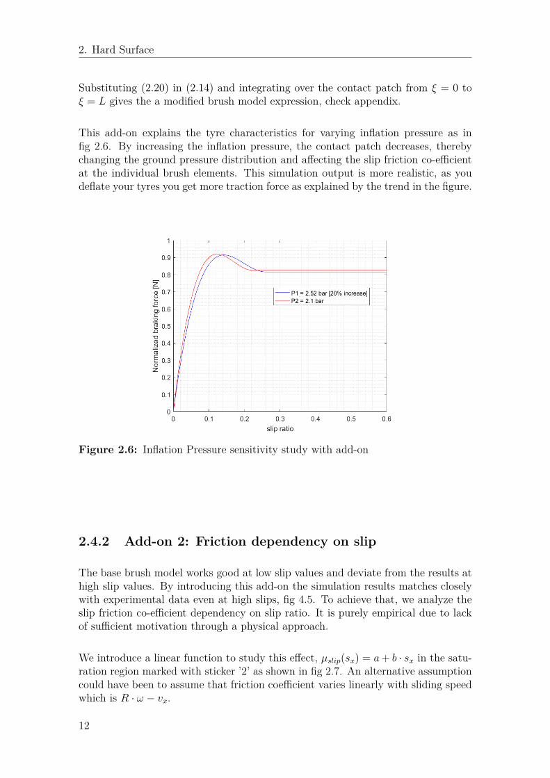
This add-on explains the tyre characteristics for varying inflation pressure as infig 2.6. By increasing the inflation pressure, the contact patch decreases, therebychanging the ground pressure distribution and affecting the slip friction co-efficientat the individual brush elements. This simulation output is more realistic, as youdeflate your tyres you get more traction force as explained by the trend in the figure.

Figure 2.6: Inflation Pressure sensitivity study with add-on

2.4.2 Add-on 2: Friction dependency on slip

The base brush model works good at low slip values and deviate from the results athigh slip values. By introducing this add-on the simulation results matches closelywith experimental data even at high slips, fig 4.5. To achieve that, we analyze theslip friction co-efficient dependency on slip ratio. It is purely empirical due to lackof sufficient motivation through a physical approach.

We introduce a linear function to study this effect, µslip(sx) = a+ b · sx in the satu-ration region marked with sticker ’2’ as shown in fig 2.7. An alternative assumptioncould have been to assume that friction coefficient varies linearly with sliding speedwhich is R · ω − vx.

12

2. Hard Surface

(a) (b)

Figure 2.7: (a): Base Brush model, (b): Brush model with Add on-2

The output characteristics with add on activated is approximated more accuratelyto the measurement data, see fig 4.5. The user has flexibility to run the simulationswith or without add ons and also combining the add ons.

2.5 Rolling Resistance Modelling

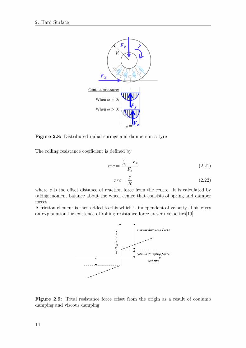
2.5.1 Spring Damper approach for rolling resistanceDifferent concepts can be used to model rolling resistance. In this section, rollingresistance is modelled assuming radial spring and damper elements extending fromrim to the outer diameter of the tyre throughout the circumference[10]. As shown infigure 2.8, the springs compress upon entering the contact patch and recover whileleaving. The energy dissipation occurs in the damper elements and this leads toadditional torque requirement for maintaining constant wheel speed.

13

2. Hard Surface

Figure 2.8: Distributed radial springs and dampers in a tyre

The rolling resistance coefficient is defined by

rrc =TRl− FxFz

(2.21)

rrc = e

R(2.22)

where e is the offset distance of reaction force from the centre. It is calculated bytaking moment balance about the wheel centre that consists of spring and damperforces.A friction element is then added to this which is independent of velocity. This givesan explanation for existence of rolling resistance force at zero velocities[19].

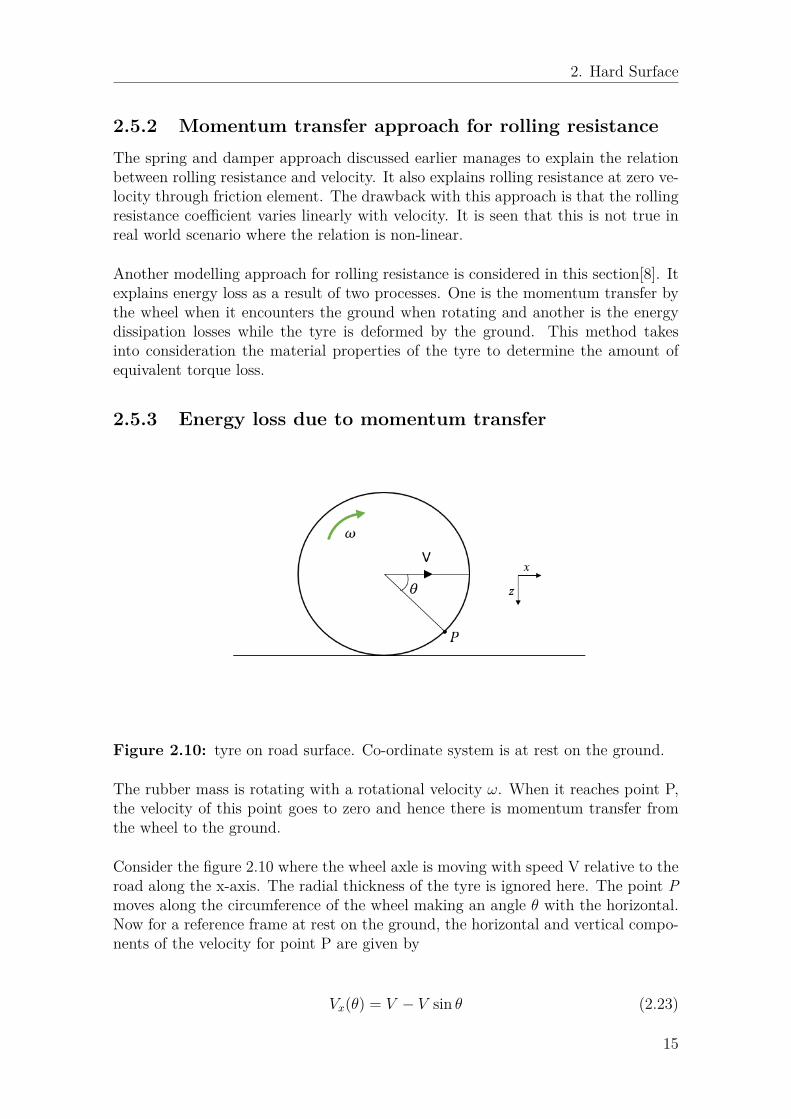
Figure 2.9: Total resistance force offset from the origin as a result of coulumbdamping and viscous damping

14

2. Hard Surface

2.5.2 Momentum transfer approach for rolling resistanceThe spring and damper approach discussed earlier manages to explain the relationbetween rolling resistance and velocity. It also explains rolling resistance at zero ve-locity through friction element. The drawback with this approach is that the rollingresistance coefficient varies linearly with velocity. It is seen that this is not true inreal world scenario where the relation is non-linear.

Another modelling approach for rolling resistance is considered in this section[8]. Itexplains energy loss as a result of two processes. One is the momentum transfer bythe wheel when it encounters the ground when rotating and another is the energydissipation losses while the tyre is deformed by the ground. This method takesinto consideration the material properties of the tyre to determine the amount ofequivalent torque loss.

2.5.3 Energy loss due to momentum transfer

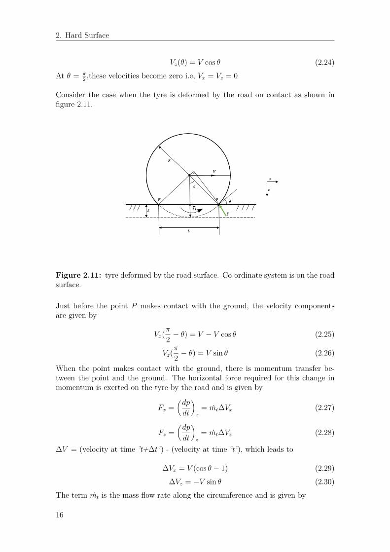
Figure 2.10: tyre on road surface. Co-ordinate system is at rest on the ground.

The rubber mass is rotating with a rotational velocity ω. When it reaches point P,the velocity of this point goes to zero and hence there is momentum transfer fromthe wheel to the ground.

Consider the figure 2.10 where the wheel axle is moving with speed V relative to theroad along the x-axis. The radial thickness of the tyre is ignored here. The point Pmoves along the circumference of the wheel making an angle θ with the horizontal.Now for a reference frame at rest on the ground, the horizontal and vertical compo-nents of the velocity for point P are given by

Vx(θ) = V − V sin θ (2.23)

15

2. Hard Surface

Vz(θ) = V cos θ (2.24)At θ = π

2 ,these velocities become zero i.e, Vx = Vz = 0

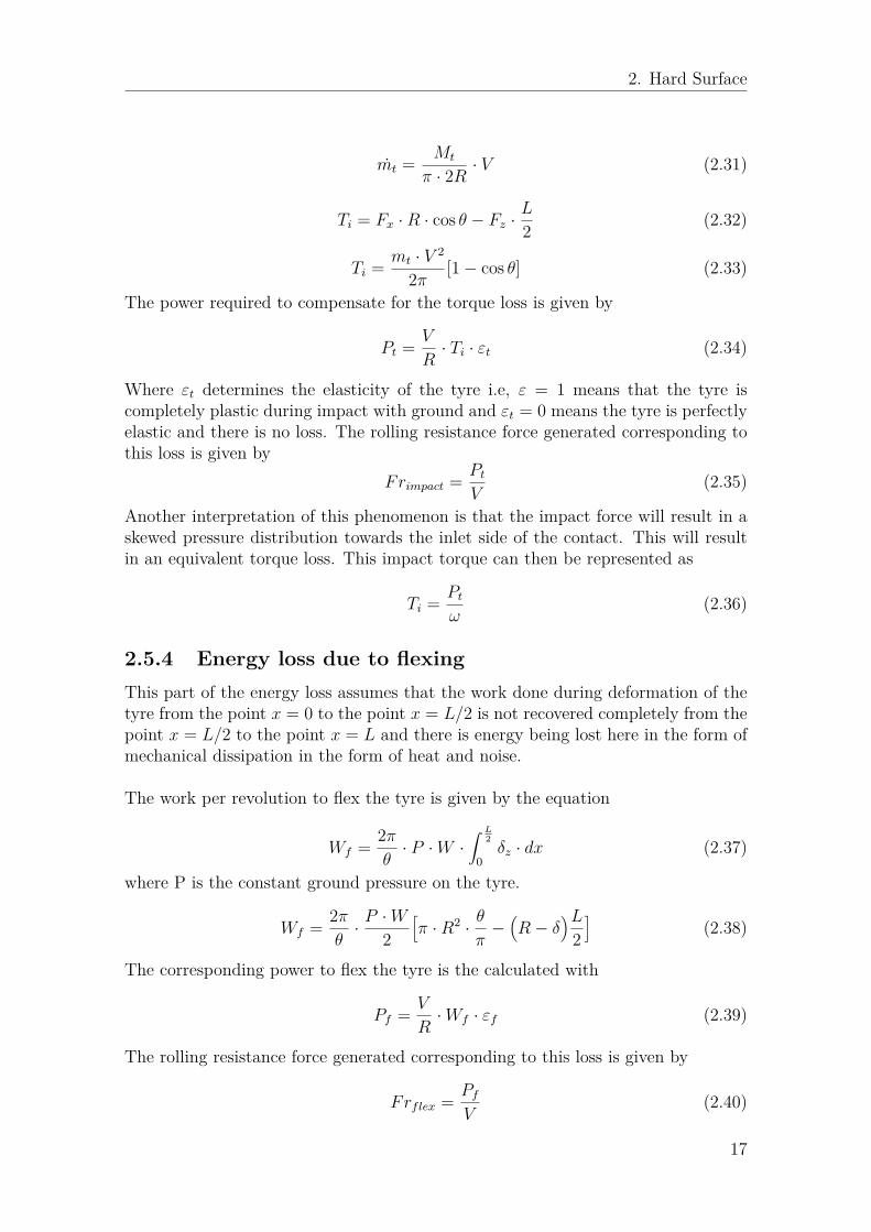
Consider the case when the tyre is deformed by the road on contact as shown infigure 2.11.

Figure 2.11: tyre deformed by the road surface. Co-ordinate system is on the roadsurface.

Just before the point P makes contact with the ground, the velocity componentsare given by

Vx(π

2 − θ) = V − V cos θ (2.25)

Vz(π

2 − θ) = V sin θ (2.26)

When the point makes contact with the ground, there is momentum transfer be-tween the point and the ground. The horizontal force required for this change inmomentum is exerted on the tyre by the road and is given by

Fx =(dp

dt

)x

= mt∆Vx (2.27)

Fz =(dp

dt

)z

= mt∆Vz (2.28)

∆V = (velocity at time ’t+∆t’) - (velocity at time ’t’), which leads to

∆Vx = V (cos θ − 1) (2.29)∆Vz = −V sin θ (2.30)

The term mt is the mass flow rate along the circumference and is given by

16

2. Hard Surface

mt = Mt

π · 2R · V (2.31)

Ti = Fx ·R · cos θ − Fz ·L

2 (2.32)

Ti = mt · V 2

2π [1− cos θ] (2.33)

The power required to compensate for the torque loss is given by

Pt = V

R· Ti · εt (2.34)

Where εt determines the elasticity of the tyre i.e, ε = 1 means that the tyre iscompletely plastic during impact with ground and εt = 0 means the tyre is perfectlyelastic and there is no loss. The rolling resistance force generated corresponding tothis loss is given by

Frimpact = PtV

(2.35)

Another interpretation of this phenomenon is that the impact force will result in askewed pressure distribution towards the inlet side of the contact. This will resultin an equivalent torque loss. This impact torque can then be represented as

Ti = Ptω

(2.36)

2.5.4 Energy loss due to flexingThis part of the energy loss assumes that the work done during deformation of thetyre from the point x = 0 to the point x = L/2 is not recovered completely from thepoint x = L/2 to the point x = L and there is energy being lost here in the form ofmechanical dissipation in the form of heat and noise.

The work per revolution to flex the tyre is given by the equation

Wf = 2πθ· P ·W ·

∫ L2

0δz · dx (2.37)

where P is the constant ground pressure on the tyre.

Wf = 2πθ· P ·W2

[π ·R2 · θ

π−(R− δ

)L2]

(2.38)

The corresponding power to flex the tyre is the calculated with

Pf = V

R·Wf · εf (2.39)

The rolling resistance force generated corresponding to this loss is given by

Frflex = PfV

(2.40)

17

2. Hard Surface

The total rolling resistance force is given by adding equations 2.35 and 2.40

Fr = Frimpact + Frflex (2.41)

Fr =(

mt

2π ·R [1− cos θ] · εt)· V 2 +

(εfR

2πθ· P ·W2

[π ·R2 · θ

π−(R− δ

)L2])

(2.42)

At V=0, the velocity dependent term Frimpact becomes zero but the velocity inde-pendent term Frflex still exists giving an offset at the origin.

18

3Soft Surface

3.1 Introduction

Soil-wheel interaction on soft surfaces is often not modeled due to the complex natureof such an interaction. Factors like the rolling resistance and braking force varysignificantly compared to hard surfaces which leads to a higher energy consumption.There is a need to capture the mechanics of this interaction for off-road vehicles orpassenger cars travelling over soft surfaces. The significant difference in this casecompared to hard surface is that the wheel sinks into the ground and this sinkagedepends on the surface properties as well as geometric properties of the wheel. Themodel becomes more complex when factors of velocity dependence and inflationpressure dependence are included. The efforts of many researchers on this subjectare explored and an attempt is made to develop a single model to predict the mainfeatures of a tyre operating in off-road scenarios[2,3,6,7,9,11,12,14].

3.1.1 Bekker’s sinkage theory

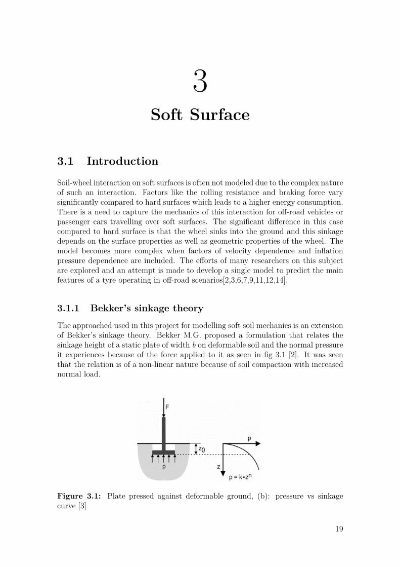
The approached used in this project for modelling soft soil mechanics is an extensionof Bekker’s sinkage theory. Bekker M.G. proposed a formulation that relates thesinkage height of a static plate of width b on deformable soil and the normal pressureit experiences because of the force applied to it as seen in fig 3.1 [2]. It was seenthat the relation is of a non-linear nature because of soil compaction with increasednormal load.

Figure 3.1: Plate pressed against deformable ground, (b): pressure vs sinkagecurve [3]

19

3. Soft Surface

Bekker’s sinkage equation is based on experimental data that includes various surfaceproperties. It is given by:

P (z) = k · zn = (k1

b+ k2) · zn (3.1)

where k1, k2 and n are termed as pressure-sinkage parameters and determined byplate sinkage tests. This equation has played a vital role in developing tyre modelsfor vehicle terrain interaction for off road applications.

The model presented in the thesis works includes both rigid tyres and flexible tyres.The rigid wheel can be assumed as a first approximation of flexible tyre.

3.2 Rigid Wheel Model

This model assumes tyre as a rigid wheel especially when the surface is softer thanthe tyre resulting in more significant deformation of the terrain than the tyre itselfprovided a minimum tyre inflation pressure is maintained. Another scenario whenthis assumption holds true is when the tyre is inflated to a point where the com-bined pressure of the stiff carcass and the inflation pressure exceed the load bearingcapacity of the terrain.

Reece [11] and Karafiath [12] asserted that equation 3.1 is inconsistent with theperception from bearing capacity theory and later modified to :

P (z) = (ck′1 + bγk′

2)(zb

)n(3.2)

where P is the pressure in Pa, z is the sinkage in m, c is the cohesion of the soil inPa, k′1 and k′2 are modified from equation 3.1 by introducing ( z

b) so that the quanti-

ties k1 and k2 become dimensionless, b is a width of the tyre in m, n is the sinkageexponent and γ is the weight density of soil in N/m3.

3.2.1 Bekker’s theory applied to wheels

The same principle can be extended to a wheel that is sinking in the ground. Therecan be two cases, one where the wheel is static on the soil surface as seen in fig 4.20aand one where the wheel is moving with a velocity of ω on the soil surface as seenin fig 4.20b.

20

3. Soft Surface

(a) (b)

Figure 3.2: (a): Static wheel on soft soil (b): Rotating wheel on soft soil

In the first case where the wheel is static, the height of the soil in front of thewheel is the same as behind the wheel making the entry angle θf and exit angleθr equal. The normal load distribution is symmetric about the wheel centre. Thesecond case however is more complicated as the wheel moves forward which makesthe soil height at the point of entry higher than the height at the point of exit.The entry and exit angles have different values and the normal load distribution isskewed. The point at which the load distribution is maximum is extended to thewheel centre and the angle between this line and the centre line is termed as θm.For any arbitrary angle θ, it can be seen from geometry that

z(θ) = R0(cos θ − cos θf ) (3.3)

3.2.2 Enhanced Bekker’s ModelThe Bekker equation 3.2 applied to wheels is the basis for the modeling approachused in this thesis [3]. The skewed load distribution in the contact area gives rise tonormal stress and shear stress along the entire contact patch as seen in figure 3.2b.

Figure 3.3: Soft surface model simulation result, typical tyre characteristics indeformable ground

21

3. Soft Surface

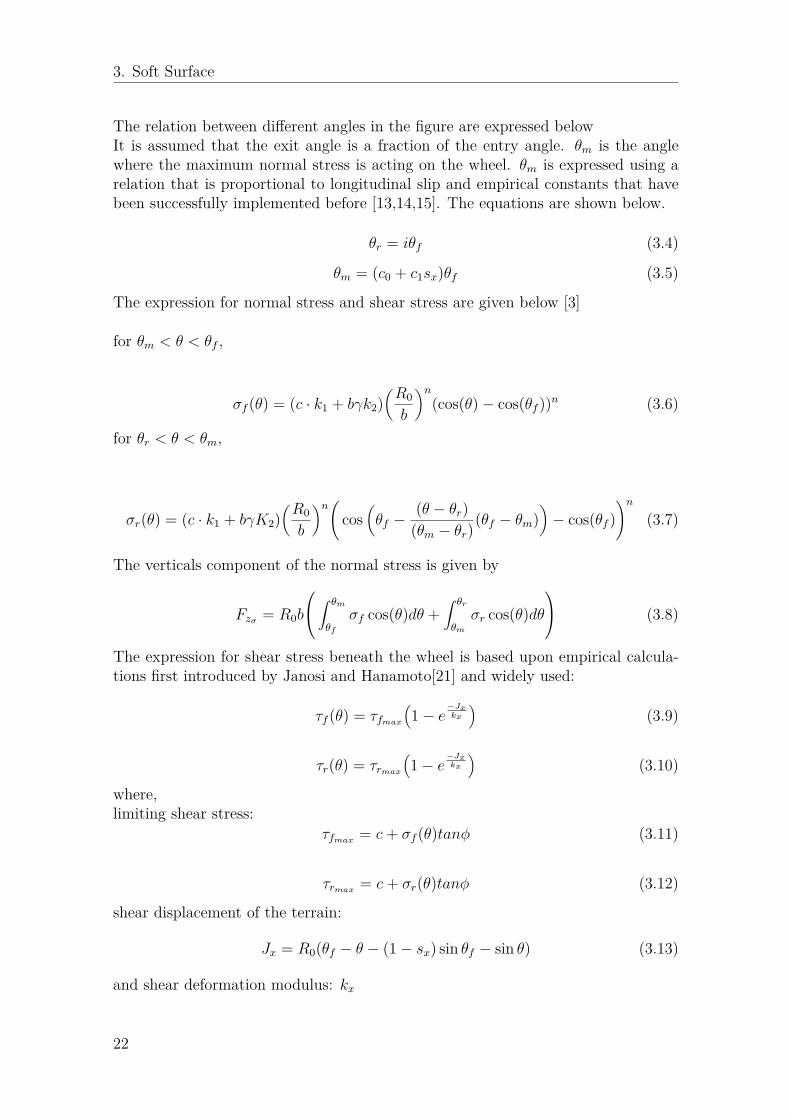
The relation between different angles in the figure are expressed belowIt is assumed that the exit angle is a fraction of the entry angle. θm is the anglewhere the maximum normal stress is acting on the wheel. θm is expressed using arelation that is proportional to longitudinal slip and empirical constants that havebeen successfully implemented before [13,14,15]. The equations are shown below.

θr = iθf (3.4)

θm = (c0 + c1sx)θf (3.5)

The expression for normal stress and shear stress are given below [3]

for θm < θ < θf ,

σf (θ) = (c · k1 + bγk2)(R0

b

)n(cos(θ)− cos(θf ))n (3.6)

for θr < θ < θm,

σr(θ) = (c · k1 + bγK2)(R0

b

)n(cos

(θf −

(θ − θr)(θm − θr)

(θf − θm))− cos(θf )

)n(3.7)

The verticals component of the normal stress is given by

Fzσ = R0b

∫ θm

θf

σf cos(θ)dθ +∫ θr

θmσr cos(θ)dθ

(3.8)

The expression for shear stress beneath the wheel is based upon empirical calcula-tions first introduced by Janosi and Hanamoto[21] and widely used:

τf (θ) = τfmax(1− e

−Jxkx

)(3.9)

τr(θ) = τrmax(1− e

−Jxkx

)(3.10)

where,limiting shear stress:

τfmax = c+ σf (θ)tanφ (3.11)

τrmax = c+ σr(θ)tanφ (3.12)

shear displacement of the terrain:

Jx = R0(θf − θ − (1− sx) sin θf − sin θ) (3.13)

and shear deformation modulus: kx

22

3. Soft Surface

The verticals component of the shear stress is given by

Fzτ = R0b

∫ θm

θf

τf sin(θ)dθ +∫ θr

θmτr sin(θ)dθ

(3.14)

The total load ′F ′z on the tyre is balanced with the vertical components given byequations (1.8) and (1.14)

Fz = Fzσ + Fzτ (3.15)

The only unknown in the set of equations leading to 1.15 is the entry angle of thewheel θf .The model calculates this value through multiple iterations to match thevertical load.

The obtained value for the angle is substituted in the equation below to find out thehorizontal force component Fx.

Fxσ = R0b

∫ θm

θf

σf sin(θ)dθ +∫ θr

θmσr sin(θ)dθ

(3.16)

Fxτ = R0b

∫ θm

θf

τf cos(θ)dθ +∫ θr

θmτr cos(θ)dθ

(3.17)

Fx = Fxσ + Fxτ (3.18)

Figure 3.4: Soft surface model simulation result, typical tyre characteristics indeformable ground plotted for vx = 5.5m/s and Fz = 4000N

The Fxσ part in the equation 3.18 constitutes the rolling resistance for this model.In other words, it is viewed as a part of the total horizontal force on the tyre and nofurther modeling is required. It is seen that there is an offest at origin in the plot3.4 which is the rolling resistance.

23

3. Soft Surface

3.2.3 Model with velocity influenceThe base model discussed in 3.2.2 does not take velocity of the vehicle into account.It has been suggested in paper [6] that traction force and rolling resistance is de-pendent on wheel speed. This section provides a velocity dependence to the basemodel that may be used if necessary. These equations represent a general trend incomparison to the results from the paper [7] but were not validated with test data.However, the empirical parameters may be tuned to match with experimental datawhen available.

Figure 3.5: Influence of velocity to the sinkage tests

The new equation is an extension of the base model with additional empirical pa-rameters.The only equations that are different from the base model are

for θm < θ < θf ,

σf (θ) = (ck1 + bρk2)(R

b

)n(cos(θ)− cos(θf ))n

(( vx1− vx

)sin( θ

v0))m

(3.19)

for θr < θ < θm,

σr(θ) = (ck1 + bρk2)(R

b

)n(cos

(θf −

(θ − θr)(θm − θr)

(θf − θm))− cos(θf )

)n(( vx

1− vx

)sin( θ

v0))m (3.20)

The constant ’m’ is tuned to obtain plot curves for varying velocity. Comparisonof plots with and without velocity dependence are done in the later parts of thereport.

24

4Validation & Results

4.1 Hard Surface

4.1.1 Fx(sx) ValidationThere are two ways in which the model is validated in the following sections.Sections 4.1.1.1 to 4.1.1.3 are validated by checking the model behaviour qualita-tively to see if the model follows the desired direction/trend by changing a singledesign parameter or operating condition at a time. Section 4.1.1.4 is validated bytaking existing data for a particular tyre and tuning the empirical parameters of themodel.

4.1.1.1 Requirements

In instances where data is missing to validate the tyre model, One way is to checkif it meets the requirements on model. These requirements are proposed by vehicledynamic researchers based on experience and found to be true for well known magicformula. The requirements of a model on hard surface are:

1. For increasing Fz, the slip where Fx,peak occurs should slightly increase∂sx,peak∂Fz

> 02. For increasing Fz, the Fx,peak should increase almost proportional to Fz, but

degressively∂Fx,peak∂Fz

> 0,∂2Fx,peak∂F 2

z≤ 0

3. For increasing Fz, the longitudinal stiffness Cx should increase almost propor-tionally, but degressively∂Cx∂Fz

> 0,∂2Cx∂F 2

z< 0

4. For increasing Pinflation, the rolling resistance coefficient should decrease∂rrc∂Pinfl

< 0

5. The model should be possible to verify experiment data

4.1.1.2 Requirements verification

Simulation output behaviourThe simulation results of the tyre-brush model are in agreement with the require-ments listed in previous section. The fig 4.1 explains the requirements 1 to 3 listed

25

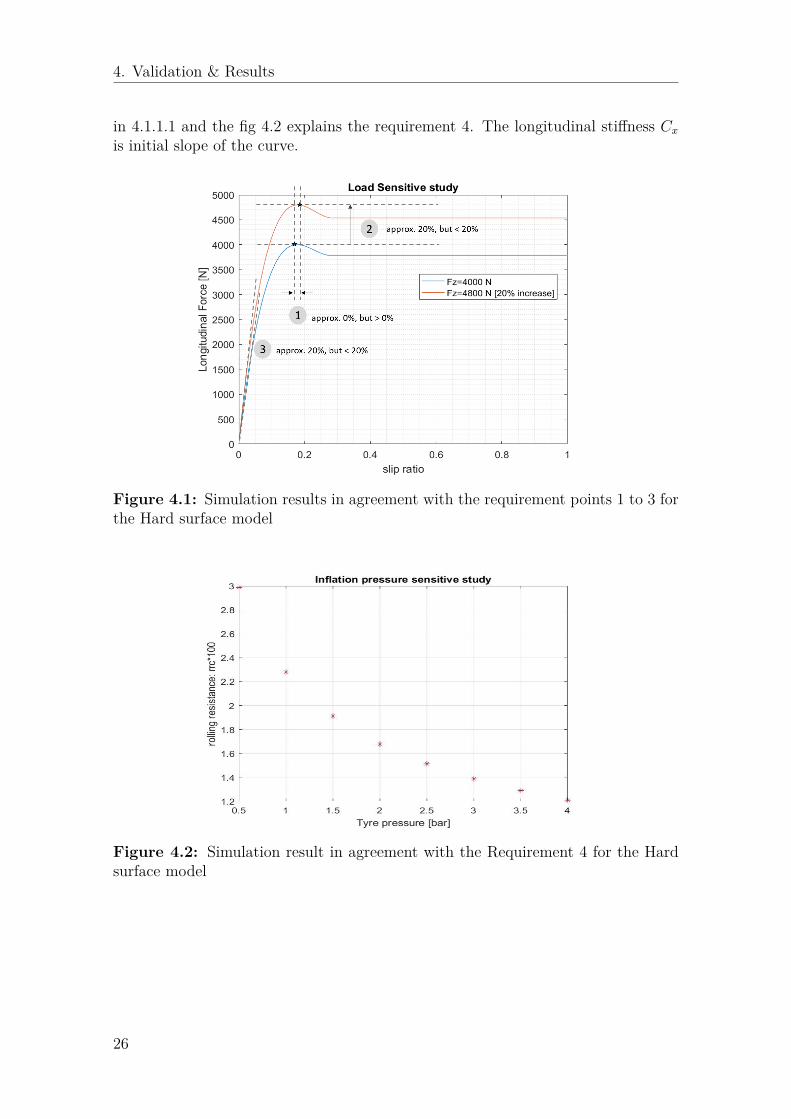
4. Validation & Results

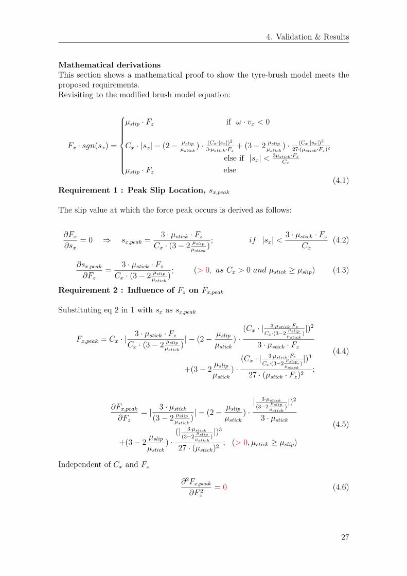
in 4.1.1.1 and the fig 4.2 explains the requirement 4. The longitudinal stiffness Cxis initial slope of the curve.

Figure 4.1: Simulation results in agreement with the requirement points 1 to 3 forthe Hard surface model

Figure 4.2: Simulation result in agreement with the Requirement 4 for the Hardsurface model

26

4. Validation & Results

Mathematical derivationsThis section shows a mathematical proof to show the tyre-brush model meets theproposed requirements.Revisiting to the modified brush model equation:

Fx · sgn(sx) =

µslip · Fz if ω · vx < 0

Cx · |sx| − (2− µslipµstick

) · (Cx·|sx|)2

3·µstick·Fz+ (3− 2 µslip

µstick) · (Cx·|sx|)3

27·(µstick·Fz)2

else if |sx| < 3µstick·FzCx

µslip · Fz else(4.1)

Requirement 1 : Peak Slip Location, sx,peak

The slip value at which the force peak occurs is derived as follows:

∂Fx∂sx

= 0 ⇒ sx,peak = 3 · µstick · FzCx · (3− 2 µslip

µstick) ; if |sx| <

3 · µstick · FzCx

(4.2)

∂sx,peak∂Fz

= 3 · µstick · FzCx · (3− 2 µslip

µstick) ; (> 0, as Cx > 0 and µstick ≥ µslip) (4.3)

Requirement 2 : Influence of Fz on Fx,peak

Substituting eq 2 in 1 with sx as sx,peak

Fx,peak = Cx · |3 · µstick · Fz

Cx · (3− 2 µslipµstick

) | − (2− µslipµstick

) ·(Cx · | 3·µstick·Fz

Cx·(3−2µslipµstick

)|)2

3 · µstick · Fz

+(3− 2 µslipµstick

) ·(Cx · | 3·µstick·Fz

Cx·(3−2µslipµstick

)|)3

27 · (µstick · Fz)2 ;

(4.4)

∂Fx,peak∂Fz

= | 3 · µstick(3− 2 µslip

µstick) | − (2− µslip

µstick) ·| 3·µstick

(3−2µslipµstick

)|)2

3 · µstick

+(3− 2 µslipµstick

) ·(| 3·µstick

(3−2µslipµstick

)|)3

27 · (µstick)2 ; (> 0, µstick ≥ µslip)

(4.5)

Independent of Cx and Fz

∂2Fx,peak∂F 2

z

= 0 (4.6)

27

4. Validation & Results

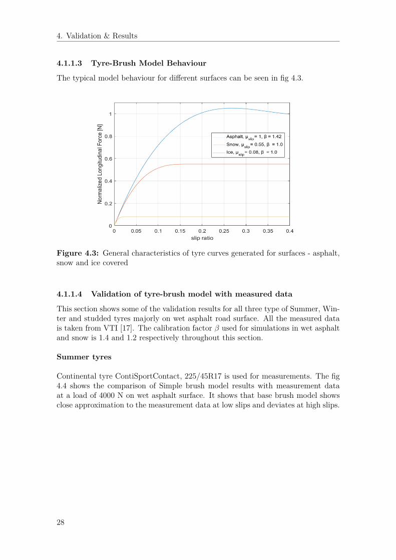
4.1.1.3 Tyre-Brush Model Behaviour

The typical model behaviour for different surfaces can be seen in fig 4.3.

Figure 4.3: General characteristics of tyre curves generated for surfaces - asphalt,snow and ice covered

4.1.1.4 Validation of tyre-brush model with measured data

This section shows some of the validation results for all three type of Summer, Win-ter and studded tyres majorly on wet asphalt road surface. All the measured datais taken from VTI [17]. The calibration factor β used for simulations in wet asphaltand snow is 1.4 and 1.2 respectively throughout this section.

Summer tyres

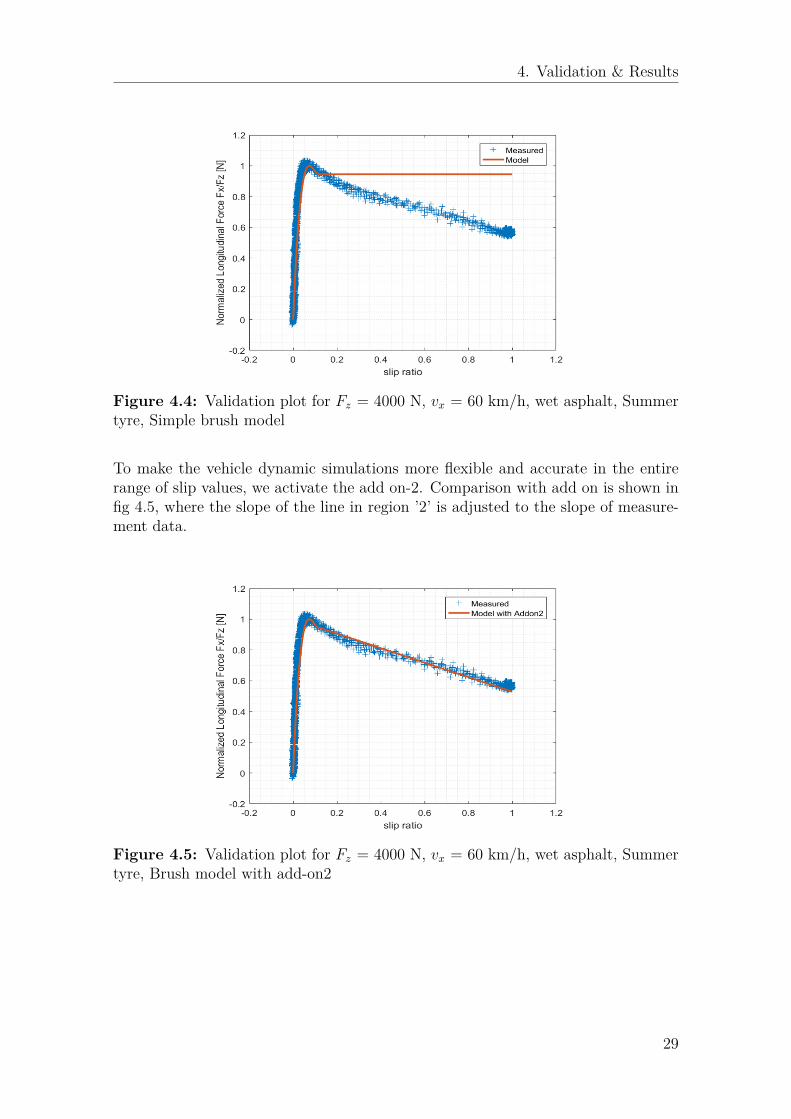
Continental tyre ContiSportContact, 225/45R17 is used for measurements. The fig4.4 shows the comparison of Simple brush model results with measurement dataat a load of 4000 N on wet asphalt surface. It shows that base brush model showsclose approximation to the measurement data at low slips and deviates at high slips.

28

4. Validation & Results

Figure 4.4: Validation plot for Fz = 4000 N, vx = 60 km/h, wet asphalt, Summertyre, Simple brush model

To make the vehicle dynamic simulations more flexible and accurate in the entirerange of slip values, we activate the add on-2. Comparison with add on is shown infig 4.5, where the slope of the line in region ’2’ is adjusted to the slope of measure-ment data.

Figure 4.5: Validation plot for Fz = 4000 N, vx = 60 km/h, wet asphalt, Summertyre, Brush model with add-on2

29

4. Validation & Results

Winter tyres

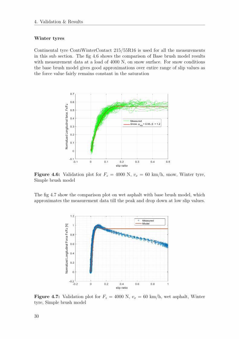
Continental tyre ContiWinterContact 215/55R16 is used for all the measurementsin this sub section. The fig 4.6 shows the comparison of Base brush model resultswith measurement data at a load of 4000 N, on snow surface. For snow conditionsthe base brush model gives good approximations over entire range of slip values asthe force value fairly remains constant in the saturation

Figure 4.6: Validation plot for Fz = 4000 N, vx = 60 km/h, snow, Winter tyre,Simple brush model

The fig 4.7 show the comparison plot on wet asphalt with base brush model, whichapproximates the measurement data till the peak and drop down at low slip values.

Figure 4.7: Validation plot for Fz = 4000 N, vx = 60 km/h, wet asphalt, Wintertyre, Simple brush model

30

4. Validation & Results

The model is made flexible at high slips by activating the add on-2 and the resultsare shown in fig 4.8

Figure 4.8: Validation plot for Fz = 4000 N, vx = 60 km/h, wet asphalt, Wintertyre, Brush model with add on-2

Studded tyres

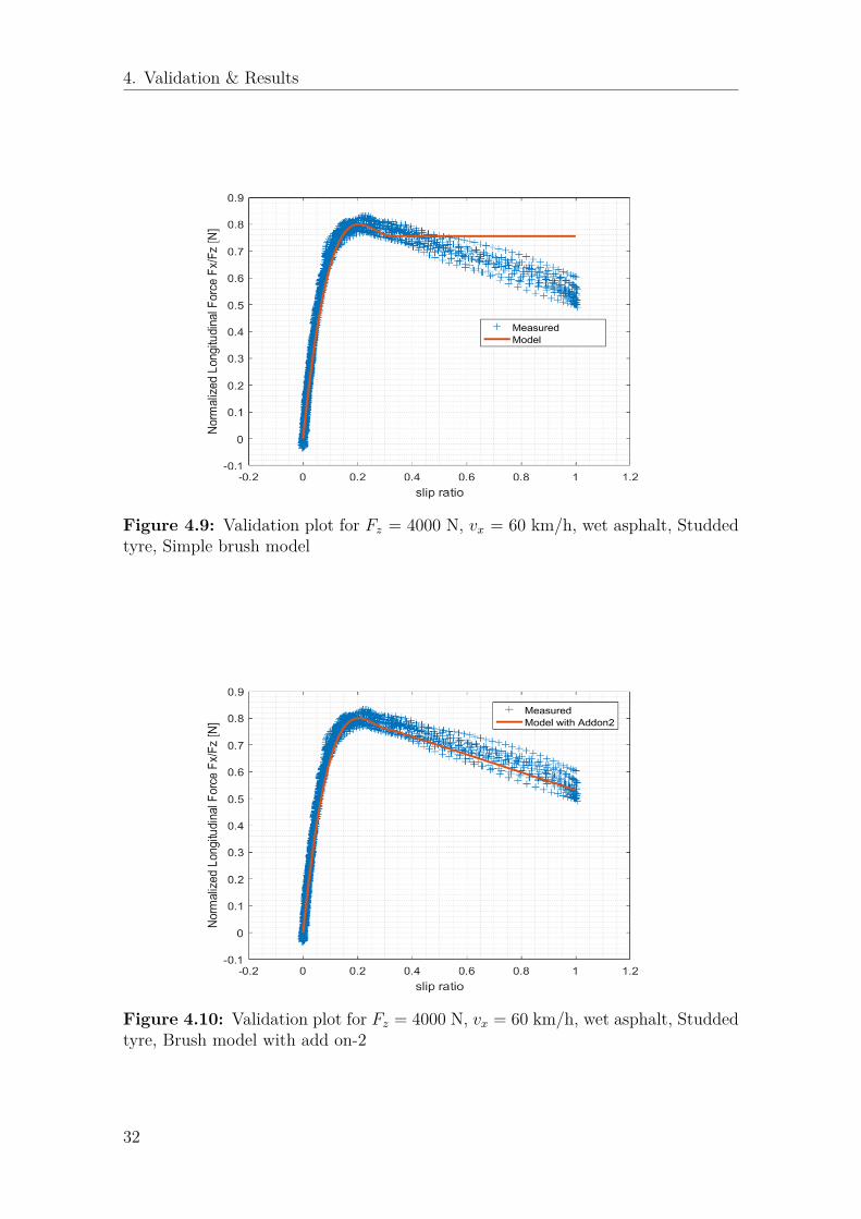
Gislaved Nordfrost 3, 215/55R16 tyre is used for all measurement data in this subsection. Similarly to summer and winter tyres, the base brush model gives goodapproximation at low slip values and activating the add on-2 gives better approxi-mation at high slips. The results are depicted in 4.9 for base model and 4.10 for themodel with add on.

For the cases where pure physical approach is desired, one can use the base brushmodel which gives good approximation of the model till the saturation is reached.Most of the vehicle dynamic simulations are performed for low slip conditions andthe base model gives good results.

The model with add ons gives the user more flexibility to run the simulations inentire slip ranges by adjusting some empirical constants. To conclude, the improvedbrush model is flexible for the user as per the requirements.

31

4. Validation & Results

Figure 4.9: Validation plot for Fz = 4000 N, vx = 60 km/h, wet asphalt, Studdedtyre, Simple brush model

Figure 4.10: Validation plot for Fz = 4000 N, vx = 60 km/h, wet asphalt, Studdedtyre, Brush model with add on-2

32

4. Validation & Results

4.1.2 Rolling Resistance validation

4.1.2.1 Requirements for rolling resistance model

Certain criteria are expected to be met by the rolling resistance model based onprevious researches and general trends observed in measurement data. This providesa good base to validate the model when obtaining experimental data is difficult. Themain requirements for the rolling resistance model are listed below continuing to thelist from the 4.1.1.1.

6. Rolling resistance coefficient varies quadratically with vehicle velocity from itsvalue at zero velocity.

7. There is a non-zero value for rolling resistance coefficient at zero velocity.

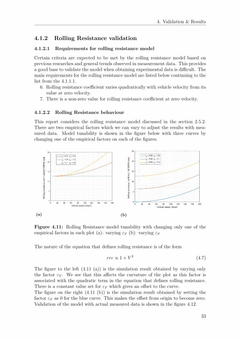
4.1.2.2 Rolling Resistance behaviour

This report considers the rolling resistance model discussed in the section 2.5.2.There are two empirical factors which we can vary to adjust the results with mea-sured data. Model tunability is shown in the figure below with three curves bychanging one of the empirical factors on each of the figures.

(a) (b)

Figure 4.11: Rolling Resistance model tunability with changing only one of theempirical factors in each plot (a): varying εT (b): varying εF

The nature of the equation that defines rolling resistance is of the form

rrc ∝ 1 + V 2 (4.7)

The figure to the left (4.11 (a)) is the simulation result obtained by varying onlythe factor εT . We see that this affects the curvature of the plot as this factor isassociated with the quadratic term in the equation that defines rolling resistance.There is a constant value set for εF which gives an offset to the curve.The figure on the right (4.11 (b)) is the simulation result obtained by setting thefactor εF as 0 for the blue curve. This makes the offset from origin to become zero.Validation of the model with actual measured data is shown in the figure 4.12.

33

4. Validation & Results

(a) Comparison to data fromMichelin 185/65 R15 MXL

(b) Comparison to data from Miche-lin 185/65 R15 MXV

(c) Comparison to data from Miche-lin 195/60 R15 MXV

(d) Comparison to data fromMichelin 205/50 VR16 MXW

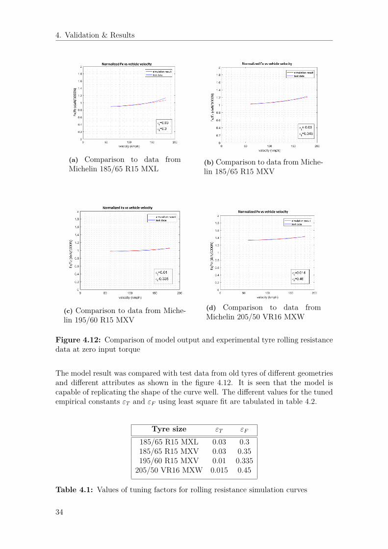
Figure 4.12: Comparison of model output and experimental tyre rolling resistancedata at zero input torque

The model result was compared with test data from old tyres of different geometriesand different attributes as shown in the figure 4.12. It is seen that the model iscapable of replicating the shape of the curve well. The different values for the tunedempirical constants εT and εF using least square fit are tabulated in table 4.2.

Tyre size εT εF

185/65 R15 MXL 0.03 0.3185/65 R15 MXV 0.03 0.35195/60 R15 MXV 0.01 0.335

205/50 VR16 MXW 0.015 0.45

Table 4.1: Values of tuning factors for rolling resistance simulation curves

34

4. Validation & Results

It should be noted that the data used here are for old tyres and are not representativeof tyres on modern cars. The values of εT and εF may change significantly for moderntyres.The values of εT and εF depend on tyre geometric properties and material properties.As seen in fig 4.12 (a) there is a higher curvature compared to fig 4.12 (c). The tyredimensions in these two cases differ largely. Depending on the build of the tyre(racetyre, passenger tyre), the tuning constants can be generalized and assumed to lie ina range. The magnitude of change in the results for these varying parameters arestudied here.

Figure 4.13: sensitivity of the model to changes in normal load by keeping geo-metric and physical parameters constant.

It is seen that the rolling resistance coefficient increases with increase in normalload. The increase in normal load causes an increase in the contact patch length.This leads to an increase in the work done due to flexing as seen in the equation2.38. Although, we do not have an explicit requirement on how rolling resistancecoefficient should vary with Fz, others have come to opposite conclusion [22].

35

4. Validation & Results

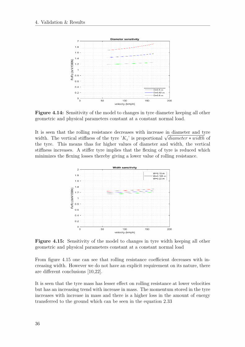
Figure 4.14: Sensitivity of the model to changes in tyre diameter keeping all othergeometric and physical parameters constant at a constant normal load.

It is seen that the rolling resistance decreases with increase in diameter and tyrewidth. The vertical stiffness of the tyre ’Kz’ is proportional

√diameter ∗ width of

the tyre. This means thas for higher values of diameter and width, the verticalstiffness increases. A stiffer tyre implies that the flexing of tyre is reduced whichminimizes the flexing losses thereby giving a lower value of rolling resistance.

Figure 4.15: Sensitivity of the model to changes in tyre width keeping all othergeometric and physical parameters constant at a constant normal load

From figure 4.15 one can see that rolling resistance coefficient decreases with in-creasing width. However we do not have an explicit requirement on its nature, thereare different conclusions [10,22].

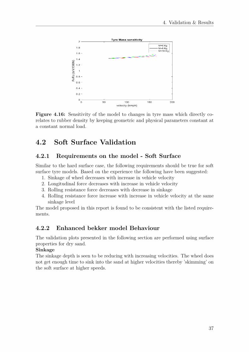
It is seen that the tyre mass has lesser effect on rolling resistance at lower velocitiesbut has an increasing trend with increase in mass. The momentum stored in the tyreincreases with increase in mass and there is a higher loss in the amount of energytransferred to the ground which can be seen in the equation 2.33

36

4. Validation & Results

Figure 4.16: Sensitivity of the model to changes in tyre mass which directly co-relates to rubber density by keeping geometric and physical parameters constant ata constant normal load.

4.2 Soft Surface Validation

4.2.1 Requirements on the model - Soft SurfaceSimilar to the hard surface case, the following requirements should be true for softsurface tyre models. Based on the experience the following have been suggested:

1. Sinkage of wheel decreases with increase in vehicle velocity2. Longitudinal force decreases with increase in vehicle velocity3. Rolling resistance force decreases with decrease in sinkage4. Rolling resistance force increase with increase in vehicle velocity at the same

sinkage levelThe model proposed in this report is found to be consistent with the listed require-ments.

4.2.2 Enhanced bekker model BehaviourThe validation plots presented in the following section are performed using surfaceproperties for dry sand.SinkageThe sinkage depth is seen to be reducing with increasing velocities. The wheel doesnot get enough time to sink into the sand at higher velocities thereby ’skimming’ onthe soft surface at higher speeds.

37

4. Validation & Results

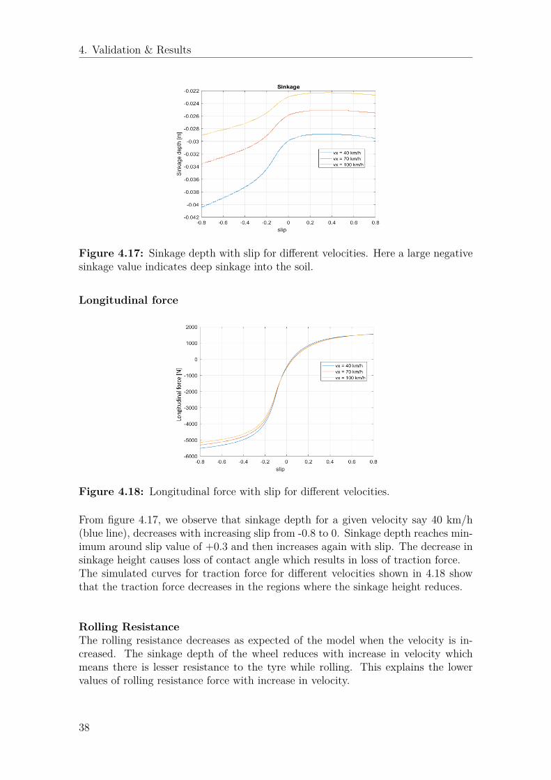
Figure 4.17: Sinkage depth with slip for different velocities. Here a large negativesinkage value indicates deep sinkage into the soil.

Longitudinal force

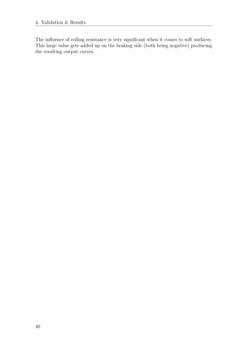
Figure 4.18: Longitudinal force with slip for different velocities.

From figure 4.17, we observe that sinkage depth for a given velocity say 40 km/h(blue line), decreases with increasing slip from -0.8 to 0. Sinkage depth reaches min-imum around slip value of +0.3 and then increases again with slip. The decrease insinkage height causes loss of contact angle which results in loss of traction force.The simulated curves for traction force for different velocities shown in 4.18 showthat the traction force decreases in the regions where the sinkage height reduces.

Rolling ResistanceThe rolling resistance decreases as expected of the model when the velocity is in-creased. The sinkage depth of the wheel reduces with increase in velocity whichmeans there is lesser resistance to the tyre while rolling. This explains the lowervalues of rolling resistance force with increase in velocity.

38

4. Validation & Results

Figure 4.19: Rolling resistance with slip for different velocities

4.2.2.1 Validation

It is often very difficult to obtain measurement data for soft surface. Validation ofthe model is done by comparing simulation results with results from the paper [3],assuming same soil parameters.The assumed soil parameters for this simulation are :

surface k1 k2 n c(Pa) φ(deg) γ(N/m3)sand 34 49.68 0.7 1150 31.1 15,696

moist loam 24.45 96.34 0.97 3300 33.7 15,196

Table 4.2: Soil property values used in the simulation for soft soil

The madel output:

(a) (b)

Figure 4.20: (a): Model output (b): Simulation result from paper[3]

The two curves in the above figure exhibit similar trends. The model developed issuccessfully able to replicate the existing simulation output. The two curves saturateat similar levels braking force levels significantly higher than the driving force levels.

39

4. Validation & Results

The influence of rolling resistance is very significant when it comes to soft surfaces.This large value gets added up on the braking side (both being negative) producingthe resulting output curves.

40

5Conclusions

5.1 Outcomes

Working models to calculate the rolling resistance and longitudinal force at the con-tact patch for hard surface and soft surface applications are built using Simulinkand Matlab.

The results presented in this report were obtained by running just the tyre modelindependently. Although this tyre model can be integrated with the main energymodel of AF consult.

Typical values of physical and emperical parameters for passenger cars is presented.

The results obtained from running the models is compared with available test dataand/or model requirements for validation.

5.2 Hard Surface

The model simulations show that the improved brush model is capable of producingreliable results up to a slip range of about 30% and typical values of β for differentsurfaces are studied and tabulated. Since most car operations are within this sliplimit it is reasonable to use the brush model up to these slip values.

The model gives closely matching results with experimental data even in the satu-ration region if the add-ons are active and some minimal parameters are tuned.

The impact loss approach for rolling resistance gives a physical explanation for thenon-linear relationship of rolling resistance value with velocity.

The report also explains the non zero rolling resistance for zero velocity. The energylost while the wheel is deformed and recovers its shape is due to mechanical energydissipation in the form of heat and noise. This value depends on the extent ofelasticity of the tyre.

41

5. Conclusions

5.3 Soft SurfaceThe developed model is consistent and gives physical explanations for the mechanicsof soil-wheel interaction when a tire goes over a deformable surface. The simulatedoutput results matches quite closely with the results published in paper[20].

Rolling resistance is a part of the model and included in the horizontal force equa-tion. This eliminates the need to have a separate model for rolling resistance.

The influence of velocity on traction and sinkage depth is an addition to the modelwhich predicts the desired trend satisfactorily.

There is a flexibility to select deformable tyre for the model which is empirical[9].Validation of this concept is not a part of this thesis work and provided as a basefor future work.

5.4 Future work1. Temperature plays an important role in tyre performance because rubber materialproperties and inflation pressure differ with varying temperature. These tempera-ture dependent effects can be added to both of the present models to improve theaccuracy of results.2. Tyre performance which includes tyre wear and loss due to vibration for differenttyre patterns can be included to the models to make it more accurate.3. The empirical parameters used in the add-ons can be generalized for differenttypes of tyres and road surfaces by tuning the model with larder sets of test datawhen available.4. The rolling resistance model for hard surfaces can be developed further by pro-viding a physical explanation for the loss mechanism during flexing of tyres (sec2.5.4). Finding test data of modern tyres to tune the values of εT and εF will be ofsignificance for obtaining realistic results.5. The flexible tyre model for soft surfaces can be developed by motivating themodel with explanations based on physical principles.6. The effect of sand/soil being thrown rearwards by a spinning wheel is not cap-tured in the present model. This effect can be added to the current model to improveaccuracy.7. The computation time for running the soft soil model can be reduced by avoidingthe iterations in the future.

42

Bibliography

[1] Bengt Jacobson, Vehicle Dynamics Compendium. Chalmers University of Tech-nology, Sweden, 2016.

[2] Bekker, M. G. Theory of land locomotion : the mechanics of vehicle mobility .Ann Arbor : University of Michigan Press, [1962, 2d print.]

[3] C. Senatore, C. Sandu, Journal of Terramechanics 48 (2011) 265–276[4] Rhyne, T. B. “Development of a Vertical Stiffness Relationship for Belted

Radial Tires,” Tire Science and Technology, TSTCA, Vol. 33, no. 3, July-September 2005, pp. 136-155.

[5] Jacob Svendenius, Tire Modeling and Friction Estimation, PhD thesis, 2007,Lund University

[6] Pope RG. The effect of wheel speed on rolling resistance, Journal of Terrame-chanics 1971;8(1):51–8

[7] I. Shmulevich a, U. Mussel, D. Wolf, The effect of velocity on rigid wheelperformance, Journal of Terramechanics 35 (1998) 189–207

[8] John R.Smith and J.Charles Tracy, David S.Potter, Tire Rolling Resistance ASpeed Dependent Contribution, SAE paper 780255 (1978)

[9] Brendan J. Chan, Development of an off-road capable tire model for vehicledynamics simulations, PhD thesis, 2008, Virginia Polytechnic Institute

[10] Bharat Mohan, Redrouthu Sidharth Das, Tyre modelling for rolling resistance,Master’s thesis 2014:24, Chalmers University of Technology

[11] Reece, A. R., 1964, "Problems of Soil-Vehicle Mechanics," Land LocomotionLaboratory (USATACOM), Warren, MI

[12] Karafiath, L. L., E. A. Nowatzki, 1978, Soil Mechanics for Off-Road VehicleEngineering, Trans Tech Publications

[13] Wong JY, Reece AR. Prediction of rigid wheel performance based on analysis ofsoil–wheel stresses, part II. Performance of towed rigid wheels. J Terramechanics1967;4(2):7–25.

[14] Shibly H, Iagnemma K, Dubowsky S. An equivalent soil mechanics formulationfor rigid wheels in deformable terrain, with application to planetary explorationrovers. J Terramechanics 2005;42:1–13.

[15] Liang D, Hai-bo G, Zong D, Jian-guo T. Wheel slip-sinkage and its predictionmodel of lunar rover. J Cent South Univ Technol 2010;17:129–35.

[16] Michelin. 2001. The tyre Grip. u.o. : Michelin, 2001[17] Gaetano Fortunato et. al, Dependency of Rubber Friction on Normal Force or

Load: Theory and Experiment, Tire Science and Technology January-March2017, Vol. 45, No. 1, pp. 25-54

[18] VTI data

43

Bibliography

[19] S.K. Clark, R.N. Dodge. A handbook for the rolling resistance of pneumatictires, The university of Michigan, Ann Arbor 1979

[20] C. Senatore, C. Sandu. Off-road tire modeling and the multi-pass effect forvehicledynamics simulation, Virginia Tech, Blacksburg 2011

[21] Janosi Z, Hanamoto B. Analytical determination of drawbar pull as a func-tion of slip for tracked vehicles in deformable soils. In: Proceedings of the 1stinternational conference on terrain-vehicle systems, Turin, Italy; 1961

[22] Zuzana Šabartová, A joint model of vehicle, tyres, and operation for the opti-mization of truck tyres, 4th International Tyre Colloquium 2015, pp. 177-186

44

AAppendix 1

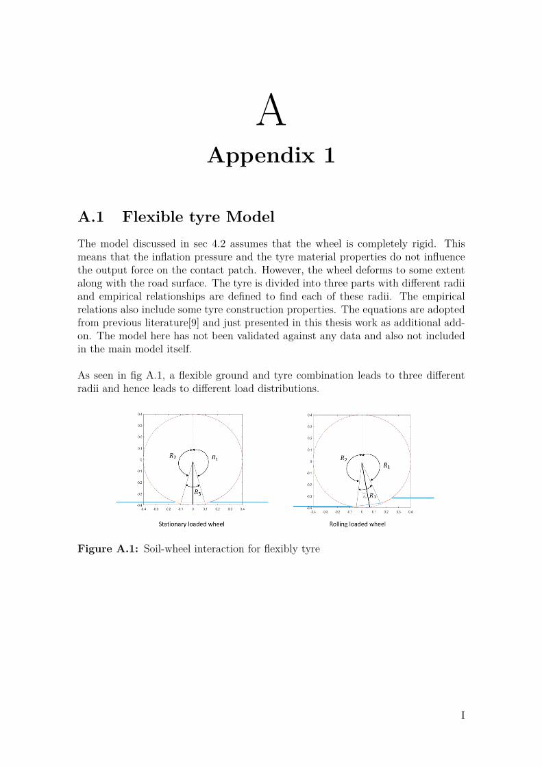
A.1 Flexible tyre ModelThe model discussed in sec 4.2 assumes that the wheel is completely rigid. Thismeans that the inflation pressure and the tyre material properties do not influencethe output force on the contact patch. However, the wheel deforms to some extentalong with the road surface. The tyre is divided into three parts with different radiiand empirical relationships are defined to find each of these radii. The empiricalrelations also include some tyre construction properties. The equations are adoptedfrom previous literature[9] and just presented in this thesis work as additional add-on. The model here has not been validated against any data and also not includedin the main model itself.

As seen in fig A.1, a flexible ground and tyre combination leads to three differentradii and hence leads to different load distributions.

Figure A.1: Soil-wheel interaction for flexibly tyre

I

A. Appendix 1

Figure A.2: Different angles formed during soil-wheel interaction on soft surface

The normal stress on the contact patch is given by the following equations :for θe < θ < θf ,

σf1(θ) = (cK1 + bρK2)[R2

(θ

b

)(cos θ − cos θe)

]n(A.1)

for θm < θ < θf ,

σf2(θ) = (cK1 + bρK2)[R1

(θ

b

)(cos θ − cos θe)

]n(A.2)

for θr < θ < θm,

σr1(θ) = (cK1 + bρK2)

R1

(θ

b

)[cos

(θe −

(θ − θb)(θe − θm)θm − θb

)− cos θe

]n

(A.3)

for θb < θ < θr,

σr2(θ) = (cK1 + bρK2)

R3

(θ

b

)[cos

(θe −

(θ − θb)(θe − θm)θm − θb

)− cos θe

]n

(A.4)

The verticals component of the normal stress is given by

Fzσ = R2b∫ θf

θeσf cos (θ)dθ +R1b

∫ θm

θf

σr cos(θ)dθ

+R1b∫ θr

θmσf cos(θ)dθ +R3b

∫ θb

θrσr cos(θ)dθ

(A.5)

Similarly, the expression for shear stress

II

A. Appendix 1

τf 1,2(θ) = τfmax(1− e

−Jx1,2kx

)(A.6)

τr3,4(θ) = τrmax(1− e

−Jx3,4kx

)(A.7)

where

τf1,2max = c+ σf 1,2(θ)tanφ (A.8)

τf3,4max = c+ σf 3,4(θ)tanφ (A.9)

Jx1,2 = R(θf 1,2 − θ − (1− sx) sin θf 1,2 − sin θ) (A.10)

Jx3,4 = R(θf3,4 − θ − (1− sx) sin θf 3,4 − sin θ) (A.11)

III

A. Appendix 1

A.2 User manual for simulink modelThe model for computation of rolling resistance force and tractive force generatedon the contact parch are combined into one Simulink module. A simplified view ofthe main blocks is shown in the figure A.3.The developed tyre models are run independently (outside of the AF energy model).The input values are loaded as constant values for running the model. When inte-grated into the main energy model, some of these inputs become dynamic inputscoming in from the main vehicle model.

Figure A.3: Simulink model of hard surface

The model takes in inputs for normal load(Fz) and vehicle velocity(vx) in the formof constant blocks. Slip(sx) is given as a ramp input here ranging between -1 to +1.However, the model is flexible to take in dynamic inputs(for Fz,vx) from the mainvehicle model while running a real simulation and calculate slip with the availablewheel speed(ω) from the main vehicle model. Other parameters are scripted in aseparate Matlab file called (initialize.m) that is executed at the beginning of everyrun. The model parameters are represented in the figure A.5.

The first function block contains equations to compute the contact patch length androlling resistance force.The contact patch length is then sent to the second block which contains the brushmodel equations to compute longitudinal force.These values are plotted with normalized Fx

(FxFz

)on the x-axis and longitudinal

slip (sx) on the y-axis and saved in the workspace.

Note: It is not possible to use the SYMS command inside a function to perform in-tegrations in the brush model equation. The integration was performed separatelyand the result was copied into the function block.

Sensitivity scriptThe sensitivity.m script contains plots for model sensitivity with different param-eters. Depending on what parameter is studied, the user has to comment out the

IV

A. Appendix 1

relevant inputs in the initialize.m file so that the inputs are taken from the sensitiv-ity.m file instead. The script has an execution command that will run the initialize.mfile and the Simulink model file and produce the required plots. This holds good forthe other sensitivity scripts as wellfiles associated with hard surface and rolling resistance

• Brushmodelnonsym.xls- main simulink model for hard surface and rolling re-sistance

• Initialize.m - initializes input parameters for both hard surface and rollingresistance

• sensitivity.m - to produce plots that check model sensitivity with various pa-rameters for hard surface model

• RRsensitivity.m - to produce plots that check model sensitivity with variousparameters for rolling resistance

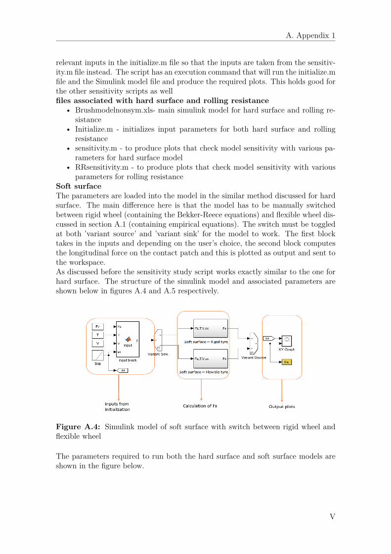
Soft surfaceThe parameters are loaded into the model in the similar method discussed for hardsurface. The main difference here is that the model has to be manually switchedbetween rigid wheel (containing the Bekker-Reece equations) and flexible wheel dis-cussed in section A.1 (containing empirical equations). The switch must be toggledat both ’variant source’ and ’variant sink’ for the model to work. The first blocktakes in the inputs and depending on the user’s choice, the second block computesthe longitudinal force on the contact patch and this is plotted as output and sent tothe workspace.As discussed before the sensitivity study script works exactly similar to the one forhard surface. The structure of the simulink model and associated parameters areshown below in figures A.4 and A.5 respectively.

Figure A.4: Simulink model of soft surface with switch between rigid wheel andflexible wheel

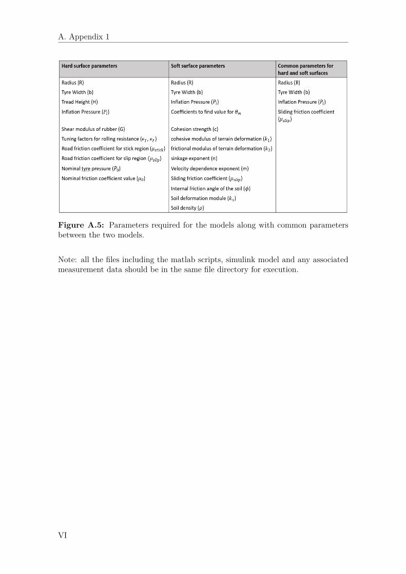
The parameters required to run both the hard surface and soft surface models areshown in the figure below.

V

A. Appendix 1

Figure A.5: Parameters required for the models along with common parametersbetween the two models.

Note: all the files including the matlab scripts, simulink model and any associatedmeasurement data should be in the same file directory for execution.

VI

A. Appendix 1

A.3 Matlab scripts

A.3.1 initialization - hard surface and rolling resistance

Some clean upclc; clear all; close all;

Contents• %%%% Simulation parameters %%%%%%%%%%%%%%%%%%%%%%%• Initialization Parameters• Road properties• For mu varying with presure• Rolling Resistance

%%%% Simulation parameters %%%%%%%%%%%%%%%%%%%%%%%sampleTime = 0.01; % Simulation Step Size [s]simTime = 10; % Simulation end time [s]

Initialization ParametersR = 0.611/2; % Radius of the tyre in mW = 0.205; % width of tyre in mP = 2.5; % Inflation pressure in bars or daN/cm^2H = 0.01;%/(a4*(Fz/Fz0)+1-a4); % Tread height in m%V = 13.88;Fz = 5000;

a=1.5;d = 200; % vertical damping stiffness of tyrec = 200; % tyre vertical spring stiffness (no influence)G = 1.1*8.63e04*a; % Longitudinal stiffness of the tyre

Road propertiesa1=1;a0=1;

mu_stk = a1; % friction co-efficient in stick regionmu_slp = a1/a0; % friction co-efficient in slip region

For mu varying with presureP0 = 10e04;mu0 = mu_stk/a0;mu1 = 0.12;

VII

A. Appendix 1

Rolling Resistance

M =9.4; % kgjt = 0.014 ; % factor for impact termjf = 0.46; % factor for flexing term

A.3.2 Sensitivity - Hard surface

Contents

• Load sensitivity• Diameter sensitivity• Width Sensitivity• Inflation pressure Sensitivity• velocity influence• Surface• Inflation pressure Sensitivity

Load sensitivity

clear allclose allR = 0.3;W = 0.2;P = 2.1;V = 25;omega = 60*5/18/R;a1=1; %[1:asphalt, 0.6:snow, 0.08:Ice]a0=1.42; %[1.42:asphalt, 1:snow, 1:Ice]

% case 1Fz=6000;sim(’Brush_Model_nonsym’)figure(1)plot(sx,Fx)grid onhold on

%case 2Fz=4000;sim(’Brush_Model_nonsym’)plot(sx,Fx)xlabel(’slip ratio’) % x-axis labelylabel(’Longitudinal Force [N]’) % y-axis labellegend(’Fz=6000 N’,’Fz=4000 N’)title(’Load Sensitive study’)

VIII

A. Appendix 1

Diameter sensitivity% case 1R = 0.4;sim(’Brush_Model_nonsym’)figure(2)plot(sx,Fx)grid onhold on

%case 2R=0.3;sim(’Brush_Model_nonsym’)plot(sx,Fx)xlabel(’slip ratio’) % x-axis labelylabel(’Longitudinal Force[N]’) % y-axis labellegend(’R=0.4 m’,’R=0.3 m’)title(’Diameter senstive study’)

Width Sensitivity% case 1W = 0.25;sim(’Brush_Model_nonsym’)figure(3)plot(sx,Fx)grid onhold on

%case 2W=0.2;sim(’Brush_Model_nonsym’)plot(sx,Fx)xlabel(’slip ratio’) % x-axis labelylabel(’Longitudinal Force [N]’) % y-axis labellegend(’W=0.25 m’,’W=0.2 m’)title(’Width sensitive study’)

Inflation pressure Sensitivity% case 1P = 1.5;sim(’Brush_Model_nonsym’)figure(4)plot(sx,Fx,’b’,sx,rrc.*Fz,’-.b’)grid onhold on

IX

A. Appendix 1

%case 2P =2.5;sim(’Brush_Model_nonsym’)plot(sx,Fx,’r’,sx,rrc.*Fz,’-.r’)xlabel(’slip ratio’) % x-axis labelylabel(’Longitudinal Force [N]’) % y-axis labellegend(’P1 = 1.5 bar’,’rolling resistance at P1’,’P2 = 2.5 bar’,’rolling resistance at P2’)title(’Inflation pressure sensitive study’)

velocity influence% case 1omega = 10*5/18/R;sim(’Brush_Model_nonsym’)figure(5)plot(sx,rrc*100)grid onhold on

%case 2omega = 100*5/18/R;sim(’Brush_Model_nonsym’)plot(sx,rrc*100)xlabel(’slip ratio’) % x-axis labelylabel(’rolling resistance: rrc*100’) % y-axis labellegend(’Vx = 10 kmph’,’Vx = 100 kmph’)title(’Velocity sensitive study’)

Surfacea1=1;a0 = 1.42;omega = 60*5/18/R;

sim(’Brush_Model_nonsym’)figure(6)plot(sx,Fx)grid onhold on

a1 = 0.4;a0 = 1;sim(’Brush_Model_nonsym’)plot(sx,Fx)hold on

X

A. Appendix 1

a1 = 0.08;a0 = 1;sim(’Brush_Model_nonsym’)plot(sx,Fx)hold off

xlabel(’slip ratio’) % x-axis labelylabel(’Longitudinal Force [N]’) % y-axis labellegend(’Asphalt, mu = 1’,’Snow, mu = 0.4’,’Ice, mu = 0.08’)title(’Different Surfaces’)

Inflation pressure Sensitivity% case 1P1 = [0.5 1 1.5 2 2.5 3 3.5 4];for i = 1:length(P1)Pi = P1(i);sim(’Brush_Model_nonsym’)figure(7)plot(Pi,rrc.*100,’*’)grid onhold onendhold off

xlabel(’Tyre pressure [bar]’) % x-axis labelylabel(’rolling resistance: rrc*100’) % y-axis label%legend(’P=1.5 bar’,’P = 2.5 bar’)title(’Inflation pressure sensitive study’)

A.3.3 Rolling resistance model%close all%clear all

V=(5/18)*linspace(0,180,1000); %vehicle velocity in meters per second

v=V*18/5; %kmph%V=16.7;%vehicle velocity in meters per secondrun ’InitializeModel’%Fz = 5000;Kz = 0.0274*P*((W*2*R*10^6)^0.5) + 3.38; % in daN/mmRe = R -(Fz/Kz/10^4); % in mkmax = acos(Re/R);% in radL = 2*(R^2 - Re^2)^0.5;

XI

A. Appendix 1

%del=R-Re;alpha = asin(L/(2*R));p_g = Fz/(W*L);

for i=1:length(V)

T(i) = ((M.*V(i).^2)/(2*pi))*(1-cos(alpha));P_t(i) = V(i).*T(i)/Re;U_t(i) = P_t(i)*jt;A_f(i) = (2*pi*p_g.*W)*((pi*R^2*(alpha/pi))-(Re)*(L/2))/(alpha*2);p_f(i) = A_f(i).*V(i)/(pi*2*R);U_f(i) = p_f(i)*(jf);

rt(i) = U_t(i)./V(i)/Fz;rf(i) = U_f(i)./V(i)/Fz;rrc(i) = (rt(i)+rf(i));end

figure(1)

plot(v,rrc*(50),’r’)xlim([0,200]);ylim([0,2]);xlabel(’velocity (kmph)’);ylabel(’Fx/Fz (daN/1000)’);%title(’Simulation plot - velocity vs normalized Fx’);hold on

%loading test data% load ’rr_expt_data’% plot(x_009,y_009/10,’b’)% legend(’simulation result’,’test data’,’location’,’Northeast’)% %t = annotation(’textbox’);% %sz = t.FontSize;% %t.FontSize = 12;% grid minor% hold on

A.3.4 Sensitivity - rolling resistance

Contents• Diameter sensitivity• Width Sensitivity• Load Sensitivity• saving files

%RR sensitivityclear all

XII

A. Appendix 1

clcclose all

R = 0.622/2; % Radius of the tyre in mW = 0.185; % width of tyre in mP = 2.5; % Inflation pressure in bars or daN/cm^2H = 0.01;%/(a4*(Fz/Fz0)+1-a4); % Tread height in mM=8;Fz=5000;

figure(1)% load ’rr_expt_data’% plot(x_006,y_006/10,’b’)% legend(’simulation result’,’test data’,’location’,’Northeast’)

grid minorhold on%%mass sensitivity%case 1M=6;run ’RR’

plot(v,rrc*(50),’r’)xlim([0,200]);ylim([0,2]);xlabel(’velocity (kmph)’);ylabel(’Fx/Fz (daN/1000)’);hold on

%case 2M=8;run ’RR’

plot(v,rrc*(50),’b’)xlim([0,200]);ylim([0,2]);xlabel(’velocity (kmph)’);ylabel(’Fx/Fz (daN/1000)’);hold on

%case 3M=10;run ’RR’

plot(v,rrc*(50),’g’)xlim([0,200]);

XIII

A. Appendix 1

ylim([0,2]);xlabel(’velocity (kmph)’);ylabel(’Fx/Fz (daN/1000)’);title(’Tyre Mass sensitivity’);legend(’M=6 Kg’,’M=8 Kg’,’M=10 Kg’,’location’,’Northeast’)hold off

Diameter sensitivity

figure(2)%case 1R=0.500/2;run ’RR’

plot(v,rrc*(50),’r’)xlim([0,200]);ylim([0,2]);xlabel(’velocity (kmph)’);ylabel(’Fx/Fz (daN/1000)’);hold on

%case 2R=0.622/2;run ’RR’

plot(v,rrc*(50),’b’)xlim([0,200]);ylim([0,2]);xlabel(’velocity (kmph)’);ylabel(’Fx/Fz (daN/1000)’);hold on

%case 3R=0.800/2;run ’RR’

plot(v,rrc*(50),’g’)xlim([0,200]);ylim([0,2]);xlabel(’velocity (kmph)’);ylabel(’Fx/Fz (daN/1000)’);title(’Diameter sensitivity’);legend(’D=0.5 m’,’D=0.62 m’,’D=0.8 m’,’location’,’Northeast’)grid minorhold off

XIV

A. Appendix 1

Width Sensitivityfigure(3)%case 1W=0.15;run ’RR’

plot(v,rrc*(50),’r’)xlim([0,200]);ylim([0,2]);xlabel(’velocity (kmph)’);ylabel(’Fx/Fz (daN/1000)’);hold on

%case 2W=0.185;run ’RR’

plot(v,rrc*(50),’b’)xlim([0,200]);ylim([0,2]);xlabel(’velocity (kmph)’);ylabel(’Fx/Fz (daN/1000)’);hold on

%case 3W=0.22;run ’RR’

plot(v,rrc*(50),’g’)xlim([0,200]);ylim([0,2]);xlabel(’velocity (kmph)’);ylabel(’Fx/Fz (daN/1000)’);title(’Width sensitivity’);legend(’W=0.15 m’,’W=0.185 m’,’W=0.22 m’,’location’,’Northeast’)grid minorhold off

Load Sensitivityfigure(4)%case 1Fz=3000;run ’RR’

plot(v,rrc*(50),’r’)

XV

A. Appendix 1

xlim([0,200]);ylim([0,2]);xlabel(’velocity (kmph)’);ylabel(’Fx/Fz (daN/1000)’);hold on

%case 2Fz=5000;run ’RR’

plot(v,rrc*(50),’b’)xlim([0,200]);ylim([0,2]);xlabel(’velocity (kmph)’);ylabel(’Fx/Fz (daN/1000)’);hold on

%case 3Fz=7000;run ’RR’

plot(v,rrc*(50),’g’)xlim([0,200]);ylim([0,2]);xlabel(’velocity (kmph)’);ylabel(’Fx/Fz (daN/1000)’);title(’Normal Load sensitivity’);legend(’Load=3000 N’,’Load=5000 N’,’Load=7000 N’,’location’,’Northeast’)grid minorhold off

A.3.5 Initialization - soft soil

Some clean up

clc; clear all; close all;

Contents

• %%%% Simulation parameters %%%%%%%%%%%%%%%%%%%%%%%• Model Selection• Initialization Parameters• Flexible tyre

XVI

A. Appendix 1

%%%% Simulation parameters %%%%%%%%%%%%%%%%%%%%%%%sampleTime = 0.01; % Simulation Step Size [s]simTime = 10; % Simulation end time [s]

Initialization Parameters% Vehicle properties% Tyre properties // Continental Contitrac SUV P265/70/R17r = 0.4;b = 0.265;c0 = 0.4;c1 = 0.2;g =-0.0;

% Dry Sandc = 1150; % [Pa] cohesion strengthk1 = 34; % kc,coeffieint in bekker pressure sinkage expressionk2 = 49.68; % kp,coeffieint in bekker pressure sinkage expressionn = 0.3;%0.7; % sinkage exponentv0 = 60*5/18;v1 = 2;m = 1;%0.3 or 1; % velocity dependence exponentmu = 0.7; % sliding friction coefficient of Dry sandphi = 31.1*pi/180; %[radians], angle of internal friction of the soilkx = 0.015; % soil deformation module for zero side slip anglerho = 15696; %[N/m3] density of soil*g

% % Moist loam% c = 22670; % [Pa] cohesion strength% k1 = 3.25; % kc,coeffieint in bekker pressure sinkage expression% k2 = 4600; % kp,coeffieint in bekker pressure sinkage expression% n = 0.99; % sinkage exponent% v0 = 60*5/18;% v1 = 2;% m = 1;%0.3 or 1; % velocity dependence exponent% mu = 0.4; % sliding friction coefficient of Dry sand% phi = 22*pi/180; %[radians], angle of internal friction of the soil% kx = 0.015; % soil deformation module for zero side slip angle% rho = 1258*9.8; %[N/m3] density of soil*g

Flexible tyred0 = 0.0230; % delta, deflection in the tire [m]z0 = 0.0845; % zetab0 = 6.3579; % beta

XVII

A. Appendix 1

A.3.6 sensitivity - soft soil

Velocity sensitivity

clear allclose all

vx = 20*5/18; % 20 km/h% case 1% Rigid wheel or flexible tyre modelm0 = 1; %[1,2]=[rigid,flexible] tyre modelM0 = Simulink.Parameter(m0);sim(’Sand_Model’)figure(1)plot(sx,Fx,’b’)grid on;hold onfigure(2)plot(sx,s0,’b’)grid on;hold on% case 2m0 = 2; %[1,2]=[rigid,flexible] tyre modelM0 = Simulink.Parameter(m0);sim(’Sand_Model’)figure(1)plot(sx,Fx,’r’)figure(2)plot(sx,s0,’r’)legend(’Rigid’,’Flexible’)

clear allclose all

m0 = 1; %[1,2]=[rigid,flexible] tyre modelM0 = Simulink.Parameter(m0);%case 2vx = 40*5/18; % 100 km/hsim(’Sand_Model’)figure(3)plot(sx,Fx)grid onhold onfigure(4)plot(sx,s0)grid onhold on

XVIII

A. Appendix 1

%case 3vx = 70*5/18; % 100 km/hsim(’Sand_Model’)figure(3)plot(sx,Fx)figure(4)plot(sx,s0)

%case 4vx = 100*5/18; % 100 km/hsim(’Sand_Model’)figure(3)plot(sx,Fx)figure(4)plot(sx,s0)

% xlabel(’slip ratio’) % x-axis label% ylabel(’Longitudinal Force [N]’) % y-axis label% legend(’vx = 10 km/h’,’vx = 40 km/h’,’vx = 70 km/h’,’vx = 100 km/h’)% title(’Velocity Sensitive study’)

XIX