Embed Size (px)
Citation preview

Universitat Stuttgart - Institut fur WasserbauLehrstuhl fur Hydromechanik und Hydrosystemmodellierung
Prof. Dr.-Ing. Rainer Helmig
Diplomarbeit
Two-phase flow modeling in porous media with kinetic interphase
mass transfer processes in fractures.
Benjamin FaigleMatrikelnummer: 2218010
Stuttgart, April 2009
Examiner: Prof. Dr.-Ing. R. Helmig Tutors: Dr.-Ing. Jennifer Niessner
Dipl.-Ing. Klaus Mosthaf


I hereby certify that I have prepared this thesis independently, and that only those sources,aids and advisors that are duly noted herein have been used and / or consulted.
Signature
Date


Contents
1 Motivation 1
1.1 Introduction . . . . . . . . . . . . . . . . . . . . . . . . . . . . . . . . . . . 1
1.2 Fractured Media . . . . . . . . . . . . . . . . . . . . . . . . . . . . . . . . 1
1.3 Fracture-Matrix System . . . . . . . . . . . . . . . . . . . . . . . . . . . . 3
1.4 Exemplary Application: Nuclear Storage Site . . . . . . . . . . . . . . . . . 5
1.4.1 Gas Infiltration from Cavern . . . . . . . . . . . . . . . . . . . . . . 6
1.5 Structure of the Thesis . . . . . . . . . . . . . . . . . . . . . . . . . . . . . 7
2 Model Concepts 9
2.1 Basic Concepts . . . . . . . . . . . . . . . . . . . . . . . . . . . . . . . . . 9
2.1.1 Definitions . . . . . . . . . . . . . . . . . . . . . . . . . . . . . . . . 9
2.1.1.1 Scales . . . . . . . . . . . . . . . . . . . . . . . . . . . . . 9
2.1.1.2 Phases α – Wetting and Non-Wetting Fluids . . . . . . . . 10
2.1.1.3 Components κ . . . . . . . . . . . . . . . . . . . . . . . . 11
2.1.1.4 Porosity φ . . . . . . . . . . . . . . . . . . . . . . . . . . . 12
2.1.1.5 Saturation . . . . . . . . . . . . . . . . . . . . . . . . . . . 13
2.1.1.6 Permeability, Conductivity . . . . . . . . . . . . . . . . . . 14
2.1.2 Constitutive Relationships . . . . . . . . . . . . . . . . . . . . . . . 15
2.1.2.1 Capillarity . . . . . . . . . . . . . . . . . . . . . . . . . . . 15
2.1.2.2 Relative Permeability . . . . . . . . . . . . . . . . . . . . 17
2.1.3 Flow in Porous Media: Darcy’s Law . . . . . . . . . . . . . . . . . 18
2.1.4 Compositional Model . . . . . . . . . . . . . . . . . . . . . . . . . . 19
2.1.4.1 Diffusion . . . . . . . . . . . . . . . . . . . . . . . . . . . 19
2.1.4.2 Equilibrium Laws for Fluids . . . . . . . . . . . . . . . . . 19
2.2 Conceptual Models for Multiphase Flow . . . . . . . . . . . . . . . . . . . 22
2.2.1 Two-Phase Model . . . . . . . . . . . . . . . . . . . . . . . . . . . . 22
2.2.2 Two-Phase Two-Component Model . . . . . . . . . . . . . . . . . . 22
2.2.3 Shortcomings of the Discussed Approaches . . . . . . . . . . . . . . 23
2.3 The new Concept including Interfacial Area . . . . . . . . . . . . . . . . . 25
2.3.1 Constitutive Relationships . . . . . . . . . . . . . . . . . . . . . . . 26
2.3.1.1 Relative Permeability krα . . . . . . . . . . . . . . . . . . 26
2.3.1.2 Specific Interfacial Area awn . . . . . . . . . . . . . . . . . 26
2.3.1.3 Production/ Destruction Rate of Specific Interfacial Area . 27
2.3.1.4 Static Production Rate of Specific Interfacial Area ewn . . 29
i

3 Mathematical and Numerical Model 333.1 Balance Equations for Two-Phase-Flow - 2p . . . . . . . . . . . . . . . . . 333.2 Balance Equations for Components - 2p2c . . . . . . . . . . . . . . . . . . 353.3 Balance Equations including Interfacial Area - 2p2cia . . . . . . . . . . . . 37
3.3.1 Mass and Momentum Equations . . . . . . . . . . . . . . . . . . . . 373.3.1.1 Balances for Bulk Phases . . . . . . . . . . . . . . . . . . 383.3.1.2 Balances for the Interfaces . . . . . . . . . . . . . . . . . . 38
3.3.2 Simplified Differential Equation System . . . . . . . . . . . . . . . . 403.4 Numerical Discretization . . . . . . . . . . . . . . . . . . . . . . . . . . . . 43
3.4.1 Time Discretization . . . . . . . . . . . . . . . . . . . . . . . . . . . 433.4.2 Space Discretization . . . . . . . . . . . . . . . . . . . . . . . . . . 443.4.3 Implementation in DUMUX . . . . . . . . . . . . . . . . . . . . . . 47
4 Case Studies 494.1 Model Setups . . . . . . . . . . . . . . . . . . . . . . . . . . . . . . . . . . 49
4.1.1 Grid Generation . . . . . . . . . . . . . . . . . . . . . . . . . . . . . 504.1.2 Model Parameters . . . . . . . . . . . . . . . . . . . . . . . . . . . 51
4.1.2.1 Fluid Parameters . . . . . . . . . . . . . . . . . . . . . . . 514.1.2.2 Soil and Fracture Parameters . . . . . . . . . . . . . . . . 524.1.2.3 Model Concepts . . . . . . . . . . . . . . . . . . . . . . . 534.1.2.4 Initial and Boundary Conditions . . . . . . . . . . . . . . 53
4.2 Verification Study for the Conceptual Models . . . . . . . . . . . . . . . . 544.2.1 Homogeneous Setup - No Fracture . . . . . . . . . . . . . . . . . . . 544.2.2 Fracture-Matrix System with One Fracture . . . . . . . . . . . . . . 58
4.2.2.1 Simulatory Challenges for the Heterogeneous Setup . . . . 634.2.3 Fracture-Matrix System with Multiple Fractures . . . . . . . . . . . 66
4.2.3.1 Angular Setup . . . . . . . . . . . . . . . . . . . . . . . . 664.2.3.2 Perpendicular Setup . . . . . . . . . . . . . . . . . . . . . 69
5 Final Remarks 715.1 Summary and Conclusion . . . . . . . . . . . . . . . . . . . . . . . . . . . 715.2 Outlook . . . . . . . . . . . . . . . . . . . . . . . . . . . . . . . . . . . . . 72
A Heterogeneous Setup with one Fracture 73
ii

List of Figures
1.1 Exposed wall of fractured sandstone . . . . . . . . . . . . . . . . . . . . . . 31.2 Fractured granite with predominant fracture directions . . . . . . . . . . . 41.3 Implementation of microscale data to gain macroscale simulative results . . 8
2.1 Fractures on different lengthscales (from Silberhorn-Hemminger (2002)). . . 92.2 Definition of the REV (Bear, 1972). . . . . . . . . . . . . . . . . . . . . . . 102.3 Contact angle of different phases (Wolff, 2008). . . . . . . . . . . . . . . . 112.4 Conceptual models for fractures (Coborny et al., 1994) . . . . . . . . . . . 132.5 Averaging from microscale to macroscale (Class, 2001). . . . . . . . . . . . 132.6 Intramolecular forces and Surface tension . . . . . . . . . . . . . . . . . . . 152.7 Capillary pressure in a capillary tube (Helmig, 1997). . . . . . . . . . . . . 162.8 Capillary pressure–saturation relationships (Helmig, 1997). . . . . . . . . . 172.9 Permeability . . . . . . . . . . . . . . . . . . . . . . . . . . . . . . . . . . . 172.10 Comparison of real mixture behaviour with Raoult’s law and Henry’s law. 212.11 Two-phase model concept . . . . . . . . . . . . . . . . . . . . . . . . . . . 222.12 Two-phase two-component model concept . . . . . . . . . . . . . . . . . . 222.13 Hysteresis of capillary pressure (Niessner and Hassanizadeh, 2009). . . . . 242.14 Two-phase two-component model with interfacial-area . . . . . . . . . . . . 252.15 Comparison of the different relative permeability functions. . . . . . . . . . 272.16 Interfacial area surfaces. . . . . . . . . . . . . . . . . . . . . . . . . . . . . 282.17 Bounding curves of the fracture . . . . . . . . . . . . . . . . . . . . . . . . 292.18 Production of Interfacial Area. . . . . . . . . . . . . . . . . . . . . . . . . . 302.19 Interpolation of the static production term of interfacial area. . . . . . . . 30
3.1 Mass balance . . . . . . . . . . . . . . . . . . . . . . . . . . . . . . . . . . 333.2 Discretization of any variable u. . . . . . . . . . . . . . . . . . . . . . . . . 433.3 Box-method . . . . . . . . . . . . . . . . . . . . . . . . . . . . . . . . . . . 453.4 Box construction in two dimensions, after (Class, 2001). . . . . . . . . . . . 45
4.1 Sketches of the applied model setups. . . . . . . . . . . . . . . . . . . . . . 504.2 Simulation grid created with mesh generator ICEM CFD. . . . . . . . . . . 514.3 Comparison of the different model concepts for the homogeneous case. . . . 554.4 Temporal characteristics at an exemplary node. . . . . . . . . . . . . . . . 564.5 Mass transfer after 50 seconds. . . . . . . . . . . . . . . . . . . . . . . . . . 564.6 Mass transfer with respect to infiltration rates . . . . . . . . . . . . . . . . 574.7 Different model concepts at the beginning of the simulation.. . . . . . . . . 58
iii

4.8 Mass transfer of air . . . . . . . . . . . . . . . . . . . . . . . . . . . . . . . 594.9 Mass fractions for an exemplary node. . . . . . . . . . . . . . . . . . . . . 604.10 Capillary pressure of the different model concepts. . . . . . . . . . . . . . 604.11 Interfacial area and static production rate of interfacial area. . . . . . . . . 624.12 Saturation Sn at various nodes over the timespan of simulation. . . . . . . 634.13 Numerical obstacles . . . . . . . . . . . . . . . . . . . . . . . . . . . . . . . 644.14 Saturation Sn at one of the crucial timesteps endangering numerical stability. 654.15 Effect of the microscale diffusion length on system validity. . . . . . . . . . 654.16 Model sketch for the angular setup. . . . . . . . . . . . . . . . . . . . . . 664.17 Dependancy on the applied grid, after 6 seconds. . . . . . . . . . . . . . . 674.18 Comparison of mass transfer for both fractures. . . . . . . . . . . . . . . . 684.19 Final state of the simulation runs which includes a second fracture. . . . . 684.20 Deviance of the new concepts . . . . . . . . . . . . . . . . . . . . . . . . . 70
A.1 Final state of the simultation runs with one single fracture. . . . . . . . . . 74
iv

List of Tables
4.1 Fluid properties of the wetting and non-wetting phase. . . . . . . . . . . . 524.2 Comparison of soil properties between fracture and matrix. . . . . . . . . . 524.3 Interfacial Area Surface Coefficients. . . . . . . . . . . . . . . . . . . . . . 524.4 Boundary Curves. . . . . . . . . . . . . . . . . . . . . . . . . . . . . . . . . 534.5 Set of primary variables. . . . . . . . . . . . . . . . . . . . . . . . . . . . . 544.6 Initial and Dirichlet Boundary Conditions . . . . . . . . . . . . . . . . . 544.7 Computational expenses for a 100 second simulation run. . . . . . . . . . . 574.8 Computational expenses for the fractured case. . . . . . . . . . . . . . . . . 61
v

vi
Nomenclature
symbol definition dimensionA area [m2]aαβ volume specific interfacial area between phase α and β [m2/m3]Dκ
α molecular diffusion coefficient of compontent κ in phase α [m2/s]Dκ
α macroscale diffusion coefficient [m2/s]cκα concentration of component κ in phase α [kg/m3]
Eαβ production rate of interfacial area [1/m · s]eαβ static production rate of interfacial area [1/m]F vector of force [N ]g magnitude of gravitational constant [m/s2]g gravity vector (0, 0,−g)T [m/s2]G solution domain [−]H Henry constant [Pa−1]krα relative permeability of phase α [−]Kf hydraulic conductivity [m/s]K intrinsic permeability tensor [m2]K permeability tensor [m2]m Van Genuchten (VG) parameter [−]Mκ Molar weight of component κ [g/mol]N basis function, ansatz function [−]n Van Genuchten (VG) parameter [−]p pressure [Pa]pκ
α partial pressure of component κ in phase α [Pa]pc capillary pressure [Pa]pd Brooks–Corey (BC) parameter, denoted as the entry pressure [Pa]pα,sat saturation vapor pressure [Pa]q secondary volume flux (sources and sinks) [m3/(m3s)]qN,α neumann boundary flux of phase α [m3/(m2s)]Sα saturation of phase α [−]Se effective saturation of water [−]Sr,α residual saturation of phase α [−]t time [s]u solution variable [−]vα velocity of phase α w.r.t. the solid phase [m/s]vαβ velocity of the interface αβ w.r.t. the solid phase [m/s]V volume [m3]
vii

xκα mole fraction of component κ in phase α [−]
Xκα mass fraction of component κ in phase α [−]
Xκα,s equilibrium massfraction of component κ in phase α [−]
x, y, z coordinates [m]α Van Genuchten (VG) parameter [Pa−1]Γ Boundary of a volume of interest [−]Γαβ Areal mass density of the αβ-interface [kg/m2]∆ increment [−]ε residual [−]λ Brooks–Corey (BC) parameter [−]σ surface tension [N/m2]τ Tortuosity [−]jκα diffusive flux of component κ [kg · m4/s]jκαβ diffusive flux over the interphase αβ [kg · m4/s]µ dynamic viscosity [kg/(ms)]ν kinematic viscosity, ν = µ/ [m2/s] density [kg/m3]φ porosity [−]
Exponents:κ general componentA, W specific components air, waterm timestep¯ volume averaged quantity˜ approximated nodal valueˆ discrete nodal value˘ discretized terms seperated from nodal values uupw upwindx, y, z coordinate directions
Indices:α, β general phasei node ij neighboring nodes j to node ik sum of neighboring nodes j to node i and node in non-wetting phases solid phasew wetting phase
viii

Chapter 1
Motivation
1.1 Introduction
Flow and transport processes in porous media gain increasing attention in many natural,industrial, and even biological systems. In most cases, there is more than one fluid in-volved, which may lead to multiphase conditions. Then, phenomena such as mass transferbetween the phases or capillary forces are obtainable. Multiphase flow problems in porousmedia are manifold, and range from natural to technical problems.Taken the porous medium of the subsurface as a classical natural example, a wide rangeof possible substances may come into focus. Besides the exploitation of resources such asoil and gas, sustainable management of the groundwater requires profound knowledge ofthe underlying flow processes. Being an important resource of drinking water, the protec-tion of groundwater from harmful pollution remains an ongoing task for applied scienceand research. The plentiful sources and types of contaminants range from infiltrationthrough rainfall that is loaded with nutrients to oil spills from leaking tanks, thus reme-diation techniques have to be chosen in accordance to the problem, whereas they are atall possible. Consequently, multiphase modeling becomes essential to asses the longtermrisks, especially in the fields of anthropogenic activities such as nuclear storage, or CO2
injection into deep geological formations.Technical porous media problems cover large-scale transport processes such as dissolvedsalt intrusion through concrete which corrodes the iron reinforcement, down to small-scalegas flow composed of oil troplets and solid particles through catalytic converters, or thediffusive flow in the layers of fuel cells. All those presented problems have in common thatthey require an interdisciplinary approach comprising, amongst others, fluid mechanics,geology, thermodynamics, mathematics, and physics.
1.2 Fractured Media
Under natural conditions, all rock mass on earth is fractured to some extend, which makesfractures an important and fascinating task of research for aquifer systems. It is assumedthat fractured or even karstic fractured aquifers contribute to about 75 % or the earth’ssurface (Dietrich et al., 2005). Fractures are mechanical breaks in rocks, acting as local
1

2 CHAPTER 1. MOTIVATION
separations or discontinuity faces in a geological formation. They originate from stress ex-ceeding the rock strength around flaws, heterogeneities, and physical discontinuities. Thestrains arise from lithostatic, tectonic, and thermal stresses which induces fractures rang-ing from microscopic to continental scales, and directing in all dimensions. An exemplarypicture of a fractured sandstone is given in Figure 1.1. The understanding of fractureproperties is very important in the fields of engineering, geotechnology, and hydrogeology,as they strongly influence water or contaminant flow. The abundance of fractured materialwidens the area of application from industrial applications to petroleum, geothermal andwater supply reservoirs, as well as safety assessments for nuclear storage sites or rechargeprocesses in the unsaturated zone, to name only few.The hydraulic properties of hard rock are predominantly determined by the fractures,both by their properties and by their spatial geometry. Based on their genesis, the differ-ent kinds of fractures can be classified into geologically based groups, amongst all of themtwo are addressed here: joints and faults. Joints are dilating fractures where the roughsurfaces moved away from each other in a perpendicular direction. However, the imageof a large displacement process may lead to a misapprehension of huge void channels.Instead, larger parts of the fracture area are in contact with the opposite complementaryfracture face which thus limits the ideal of two parallel, fully displaced plates. Faults, incontrast, are shear displacement fractures with predominantly lateral movement of theadjected rocks. Due to the parallel displacement, fault surfaces are polished and markedby linear features in contrast to the ornamented surfaces of joints, and may thus producepotential pathways for fluid flow (Long et al., 1996). Since faults or joints do not usuallyconsist of one single defined fracture, fracture sets or fracture zones are of high interest inregards to fluid flow. Effective properties such as porosity or conductivity to fluid flow arehighly dependent on the connectivity of the fracture network, which in turn varies withfracture genesis. The underlying geological processes and scales of interest (see Chapter2.1.1.1) are thus crucial for the determination of fluid flow in such structures.Further problems arise if the fractures are modeled as a continuum which is an averaged
description of complex discontinuities by a set of continuous state variables, amongst them(Long et al., 1996; Dietrich et al., 2005)
• As we have seen, the exact spatial configuration and geometry of possible pathwaysas streamtubes to flow are incredibly difficult to define on smaller scales, resultingin high uncertainties.
• Dispersion, a process caused by the variation of the different pathways leading todifferent flow velocities and pathlengths, inhabits highly anisotropic behaviour alongthe fractures. It is thus questionable to tackle this phenomenom alike proceduresin porous media, whilst experimental data for fractured porous media are not yetsufficient.
• As fractures occur on every scale, it is challenging to transform effective parameteresfrom the testing laboratory to the scale of interest of the model domain.
• Flow through fractures may be accommodated using the fracture aperture, thedistance between two neighboring fracture walls, as a model parameter. However,

1.3. FRACTURE-MATRIX SYSTEM 3
Figure 1.1: Exposed wall of fractured sandstone with horizontal fractures caused by sed-iment layering and vertical fractures due to mechanical stress (Dietrich et al., 2005).
since fracture aperture is not constant in nature, its distribution has to be addressedin a statistical manner which should at best be measured in situ, in the place.
1.3 Fracture-Matrix System
As discussed above, fractures occur on a variety of lengthscales, ranging from tiny fissuresto faults and joints with considerable aperture sizes. In order to reduce the complexicityof the system, it is desirable to disregard structural information when their influencecan be detected with the help of effective parameters, while being still able to capturelarge heterogeneities. The fractured rock mass is thus assumed to be binary divided intofractures or fractured zones on the one side, and average-fractured rock, denoted as thematrix, on the other side (see the concept of an REV in Chapter 2.1.1.1, as well as Chapter2.1.3). This assumption seems reasonable, because small, unconnected fissures within therock matrix are not regarded as preferential pathways for contaminant solutes, thus donot increase flow velocity as severe as large-scale and connected fractures do. Followingtheir parallel genesis due to common stress tensors (Figure 1.2), it seems furthermorereasonable to group single fractures together to fracture zones with a defined direction toapply an continuum modeling approach. However, the simplification to a matrix which ispervaded by fractures, gives rise to even more questions (Long et al., 1996), for example:
• What is the right choice of the scale of interest, which processes are negligible, whichones of high interest?
• The contrasts of the fracture and the matrix properties are huge, conductivity differs

4 CHAPTER 1. MOTIVATION
Figure 1.2: Exposed fracture zone of a weathered granite with predominant fracturedirections, Norway.

1.4. EXEMPLARY APPLICATION: NUCLEAR STORAGE SITE 5
by several orders of magnitude. Are the processes in both parts compareable, doassumptions which are valid for porous media (i.e. slow, laminar flow; thermody-namic equilibrium) also hold for flow in fractures? Are mathematical descriptionsvalid for both parts?
• Since fractures and the matrix interact, how could both parts be connected in amodel? Fractures tend to desaturate before the pores of the matrix because ofcapillary effects, thus dry fractures act as barriers to fluid flow. However, fracturesurfaces may be sealed with minerals, thus capillary forces may be to weak to drawwater from the high-permeable fractures. This means that water as well as gasmigrate through the fracture, which now acts as pathways to fluid flow.
• Which conceptual model is appropriate for a simulatory link between the fractureand the matrix? Which numerical schemes have to be used to successfully connectthem?
After all, fracture-matrix systems represent an exciting and challenging task, both for ba-sic research as well as applied science. There is further need to investigate flow processesboth numerically and with experiments, to broaden the knowledge and to improve sys-tematic understanding of the underlying processes. In conclusion, fracture-matrix systemsare important for a large range of problems - one of them will be exemplarily addressedin the following section in little more detail.
1.4 Exemplary Application: Nuclear Storage Site
Any usage of nuclear energy requires a solution for the nuclear waste. Current politi-cal discussions about an extended production of nuclear energy to fight climate change(wether that is appropriate or not will not be addressed in this work) even sharpensthe urgent need for convenient disposal sites for spent fuel. Besides the storage in saltcavities, the focus was directed towards rock dumping sites which seems advantageouslybecause they are considered virtually impermeable. As discussed in the chapters afore,the impermeable rock mass, also denoted as “natural barrier”, is usually interlaced withfractures, and if properly connected, significant flow processes may be indeed possible.With regards to the incredible timespans where safety has to be ensured, any migrationof pollutants must be taken serious and under careful consideration. Risk assessmentover tens of thousands of years demands huge efforts for simulation technology, so basicknowledge of the underlying processes is acutely significant.While the Yucca Mountain site, a nuclear storage facility in the US, already lies above
groundwater level and thus in the unsaturated zone, most projected storage sites will belocated around 500m under the groundwater level, thus fully saturated conditions can beexpected. Observations from recent experiments from the Aspo Hard Rock Laboratoryin Sweden (Figure 1.3(a)), however, report that multiphase conditions even occur undersuch physical conditions, leading to a drastic reduction of the effective permeability inaddition to other effects. The evolution of a second gaseous phase originates on the oneside from the effect of degassing, where a pressure drop in the vicinity of the disposal
6 CHAPTER 1. MOTIVATION
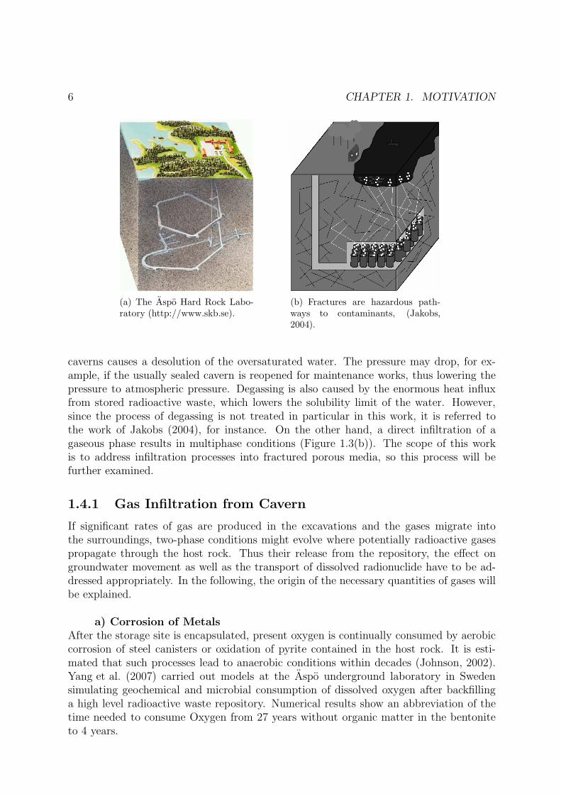
(a) The Aspo Hard Rock Labo-ratory (http://www.skb.se).
(b) Fractures are hazardous path-ways to contaminants, (Jakobs,2004).
caverns causes a desolution of the oversaturated water. The pressure may drop, for ex-ample, if the usually sealed cavern is reopened for maintenance works, thus lowering thepressure to atmospheric pressure. Degassing is also caused by the enormous heat influxfrom stored radioactive waste, which lowers the solubility limit of the water. However,since the process of degassing is not treated in particular in this work, it is referred tothe work of Jakobs (2004), for instance. On the other hand, a direct infiltration of agaseous phase results in multiphase conditions (Figure 1.3(b)). The scope of this workis to address infiltration processes into fractured porous media, so this process will befurther examined.
1.4.1 Gas Infiltration from Cavern
If significant rates of gas are produced in the excavations and the gases migrate intothe surroundings, two-phase conditions might evolve where potentially radioactive gasespropagate through the host rock. Thus their release from the repository, the effect ongroundwater movement as well as the transport of dissolved radionuclide have to be ad-dressed appropriately. In the following, the origin of the necessary quantities of gases willbe explained.
a) Corrosion of MetalsAfter the storage site is encapsulated, present oxygen is continually consumed by aerobiccorrosion of steel canisters or oxidation of pyrite contained in the host rock. It is esti-mated that such processes lead to anaerobic conditions within decades (Johnson, 2002).Yang et al. (2007) carried out models at the Aspo underground laboratory in Swedensimulating geochemical and microbial consumption of dissolved oxygen after backfillinga high level radioactive waste repository. Numerical results show an abbreviation of thetime needed to consume Oxygen from 27 years without organic matter in the bentoniteto 4 years.

1.5. STRUCTURE OF THE THESIS 7
Under such anaerobic conditions, the oxidation of iron or steel can be formulated as
3Fe + 4H2O → Fe3O4 + 4H2 . (1.1)
To guaranty the safety requirements for the installed canisters, numerous studies havebeen undertaken to estimate the corrosion rate of the applied container materials. Sincethe chemical reaction depends on the partial pressure of the present hydrogen, the tem-perature, the pH-conditions in the surroundings and the presence of water or humidity,a constant gas production rate over the vast timescale of such a storage site can not beexpected. However, results form studies with buried archaeological artifacts indicate thatcomparable rates are likely to be sustained over thousands of years, so it is reasonableto assume an average gas production rate over a time frame of the order of the canisterlifetime (Johnson et al., 2004). Nontheless, any quantities should be treated with caresince the different investigations were undertaken under diverse environments (differentrock types, timescales etc.).The range of the total gas volume that is produced per year varies between 100 −
150m3/yr.(Smart, 2008) up to 240m3/yr. (Johnson et al., 2004), and are thus high enoughto have an impact on flow behaviour and phase composition in the saturated zone. Notethat the corrosion of other alloys such as Zircalloy are not taken into account in the con-text of already high uncertainties of the steel corrosion rate, and because the total massof the alloy is magnitudes smaller than that of steel in the emplacement tunnels.
b) Radiolysis of WaterRadiolysis denotes the cleavage of a chemical bond, similar to the process of photolysis,but influenced by ionizing radiation. The products of radiolysis are molecules, ions orradicals. In the presence of water, α−, β− and γ−radiation can produce hydrogen andoxygen, hydrogen peroxide and further short-lived radical species (Rompp et al., 1999).Since the canisters effectively shield radiation over their projected lifetime of 10 000 years,significant gas production will commence after canister breaching. However, a roughbounding estimate presuming that a thin water layer covers the complete fuel surfacesyields a production rate of only 5l per year, so radiolysis can be neglected in respect tothe production rates due to corrosion (Johnson et al., 2004).
1.5 Structure of the Thesis
Adjacent to the introduction, Chapter 2 provides a general definition of the most impor-tant terms and the underlying principal physical concepts. Subsequently, an overview ofthe conceptual standard models in regards to multiphase flow is given, and the limitationsof the approach is presented. The conceptual model of the new approach is introducedin the last section, and the conceptual benefits are discussed. Chapter 3 gives a ba-sic derivation of the mathematical descriptions with respect to each of the conceptualmodels. Thus, the final governing equations as well as supplementing correlations arepresented, and the numerical implementation bridges the gap to the simulatory part ofthis work. Here, microscale properties have to be implemented in the coarser framework,and test cases for the simulations are assembled in Chapter 4, followed by a discussion ofthe results. Chapter 5 gives a summary of this work and ventures a brief perspective.

8 CHAPTER 1. MOTIVATION
Figure 1.3: Implementation of microscale data to gain macroscale simulative results, withfigures taken from Joekar-Niasar et al. (2007); Nuske (2009).

Chapter 2
Model Concepts
2.1 Basic Concepts
As discussed in the previous chapter, the structure of porous media and fracture-matrixsystems is particularly complex, and a detailed description of the geometry of the porestructure or fracture-matrix interfaces is not infeasible. In order to model such diversestructures, a continuum approach defined on a larger scale with averaged microscale prop-erties is necessary. The averageing process generates new macroscale properties such asvolume-based saturation or fluid-dependent relative permeability are generated, and mi-croscale discontinuities can no longer be identified.
2.1.1 Definitions
2.1.1.1 Scales
Theoretically, most physical processes or properties are based on attributes or interac-tions of single molecules on a very small scale, denoted in this work as the molecular
scale. To examine interactions caused by the dipolar moments of molecules, for example,incredibly large numbers of molecules would have to be considered, since 1g of pure watercontains over 1022 molecules! Thus, it is more common to use a statistical approach,
mm
µm
fracture network
groundwaterreservoir
hydrogeolocical
with rock matrix
aquifer structure
km
m
boundary layer
single fracturemm
Figure 2.1: Fractures on different lengthscales (from Silberhorn-Hemminger (2002)).
9

10 CHAPTER 2. MODEL CONCEPTS
volumeV0 =REV
Inhomogeneousmedium
Homogeneousmedium
Domain ofmicroscopiceffects
Domain ofporousmedium
physi
calpro
per
ty,
e.g.
por
osity
φ
Figure 2.2: Definition of the REV (Bear, 1972).
where molecular attributes are upscaled to fluid properties such as density, viscosity, orinterfacial tensions. Since in such a microscale scope the explicit description of moleculesvanishes, physical processes which result from molecular interaction have to be describedwith new properties such as diffusion or heat transfer coefficients. The microscale is thelargest scale where a clear spatial separation of fluid phases can be detected, and whereclear interfaces between the fluids are present. Flow in porous media can be describedon this scale by the Navier-Stokes equations for which the exact structure of the solidsurfaces needs o be described. For large systems, a larger or coarser scale is needed forthe description flow in porous media, what requires another continuum step towards amacroscale.
An averaging procedure over a representative elementary volume (REV) (Bear, 1972)introduces macroscale parameters (see the following sections), as well as constitutive rela-tionships (Chapter 2.1.2) or even new mathematical equations (Chapter 2.1.3). Originat-ing from the inability to solve the real underlying phenomena, Bear referred to them as“parameters of ignorance”, and some of the associated problems are addressed in Chapter2.2.3.On the one hand, the size of the REV must be large enough to avoid undesired fluctua-tions of, for example, grain size distribution which varies the porosity, but on the otherhand, its resolution should still be small enough to unravel dependencies of the entire flowdomain, for example fractures. While these limits can be defined for homogeneous mediausing the procedures presented in Bear (1972), it is much more complex with regardsto fracture-matrix systems because of the diverse lengthscales of the heterogeneities (seeNuske (2009); Jakobs (2004), Figure 2.1).
2.1.1.2 Phases α – Wetting and Non-Wetting Fluids
A phase denotes matter with a homogeneous chemical composition and uniform physicalproperties. Under multiphase conditions, the phases are separated by an interface across

2.1. BASIC CONCEPTS 11
θ
non−wetting phase wetting phase
> 90°
< 90°
θ
Figure 2.3: Contact angle of different phases (Wolff, 2008).
which discontinuities in the material properties exist. Phases may be differentiated ac-cording to their state of matter (solid, fluid, or gaseous), yet phase changes occur due tochanges of the conditions, e.g. a pressure drop. Based on their chemical polarity, twofluids may be immiscible on the microscale, thus creating a clear interface between thesingle phases leading to a pressure difference (see 2.1.2.1). Since there is no interfacebetween different gases, they are completely mixed within one phase.With respect to the solid matrix, the phases (α) may be classified as wetting (w) or non-wetting (n) phases. Under natural subsurface conditions, the solid matrix is usually polar(which may not hold for technical applications such as the hydrophobic diffusion-layer infuel cells), and thus the fluid with the higher polarity is more strongly attracted. Thisbehaviour is represented by the contact angle θ between the fluid-fluid interface and thesolid surface, where the fluid with an acute boundary angle (θ < 90) is referred to as thewetting fluid.Throughout this thesis, the term “phases” is only used for the fluids, air and water in
specific, while the solid phase is denoted as the “solid matrix”. “Twophase conditions” inthis thesis therefore prevail if two fluid phases exist in a porous medium, the underlyingthird phase.
2.1.1.3 Components κ
In real systems, phases are neither perfectly separated nor absolutely insoluble. There-fore, every phase consists of different chemical constituents which are present in thesystem, for example dissolved ions in saline water. Considering complex systems, werather use the concept of components which are chemically independent constituents(Atkins and De Paula, 2006). The number of components κ in a system represents theminimum number of independent constituents for the description of the phase compo-sition. It depends on the conceptional model which chemical species or mixtures aregrouped together as one component: Air, for example, can on the one hand be treatedas one component if solubility effects of air in water is the point of interest. On theother hand, air is a mixture of several components (nitrogen, oxygen, argon etc) whosecomposition defines, for example, the partial pressure. The composition of the phases isquantifiable by using the expression of mass fractions Xκ
α, which is defined as the mass ofa component over the total mass of the phase. Obviously, the sum over all components

12 CHAPTER 2. MODEL CONCEPTS
in a phase must equal one:
∑
κ
Xκα = 1 for all components κ = κ1, κ2, . . . (2.1)
However, if we are interested in the actual number of molecules with disregard to theirmasses, we can make a transition to mole fractions, describing the number of moles of thecomponent κ in phase α:
xκα =
Xκα
Mκ. (2.2)
Mκ denotes the mass of one mole of a component and corresponds to the molecular massof the substance. Like mass fractions, the mole fractions sum up to one,
∑
κ
xκα = 1 for all components κ = κ1, κ2, . . . (2.3)
Throughout this work, equations are intended to be as general as possible, thus compo-nents are generally denoted as κ. However, to improve readability, whenever the compo-nents have to be distinguished, the superscripts A and W for the components air andwater are used rather then κ1, κ2 . . . , because a two-phase system of water and air isregarded.
2.1.1.4 Porosity φ
The concept of an REV requires, among other parameters, a minimum Volume V0 toobtain a unique, non-oscillating value for the ratio φ of pore volume Vpore to total volumeVtotal. This gives the a definition of porosity:
φ =Volume of pore space within the REV
Total Volume=
Vpore
Vtotal(2.4)
In most cases, parts of the pore space is not available for fluid flow since, since not allpores are connected. Therefore, a decreased value φeff may be used for the descriptionof fluid flow. In addition, the solid phase may change with temperature or pressure vari-ations. Clay, for example, is capable of swelling or shrinking depending on water yield,hence porosity changes with soil saturation. However, the solid phase, and thus porosity,is assumed to remain constant in this work.In fracture voids, porosity is expectably equal to one. As discussed in Chapter 1, spatialvariations of fracture aperture are significant, but ought to be averaged out on the REV-scale. For the numerical model, a single fracture needs to be incorporated in the modelframework of larger grid elements, so an upscaling approach gets necessary. In addition,as discussed in Chapter 1, fractures exist on a variety of lengthscales. From the modelingperspective, complex networks of discrete fractures were transferred to a concept of frac-tured zones or water-conducting features (Figure 2.4). Those areas represent active flowsubsystems with considerably higher porosity than the surrounding rock matrix. Thus,if the term “fracture” is used in the following, it may also refer to a fracture zone. Thereal fracture aperture of several connected single fractures is, therefore, represented by anadjusted artificial porosity of a fracture zone.

2.1. BASIC CONCEPTS 13
Figure 2.4: Hydrogeological and numerical conceptual models for fractures(Coborny et al., 1994).
2.1.1.5 Saturation
Within the REV, it is not feasible to preassume the exact spatial distribution of fluidphases or the pore matrix, but the ratio of their volumes is taken into account instead.Therefore, new system parameters such as effective saturation are introduced which donot exist below the REV-scale. Under multiphase conditions, each phase can occupy acertain ratio of pore space, which can be written as:
Sα =volume of phase α in REV
volume of pore space in REV=
Vα
Vpore
(2.5)
The averaging process to the REV-scale as shown in Figure 2.5 assumes that the pore
averaging
soil matrix
liquid phase
gas phase
microscale REV
Figure 2.5: Averaging from microscale to macroscale (Class, 2001).
space in the REV is completely filled by all phases α combined, which determines thefollowing supplementary constraint:
∑
α
Sα = 1 (2.6)

14 CHAPTER 2. MODEL CONCEPTS
Displacement processes between phases are referred to as between drainage or imbibition:If a non-wetting fluid moves into a porous medium which was initially saturated withthe wetting phase, the saturation Sw of the wetting fluid will gradually decrease. Thisdrainage process may last until no further wetting fluid can be displaced, and a residualwetting saturation Sr,w remains. If this displacement process is inverted (i.e. imbibition),the non-wetting saturation converges towards the residual non-wetting saturation Sr,n.Values of residual saturations depend on the pore geometry, the heterogeneity and thedisplacement process, but also on the number of drainage and imbibition cycles. Inaddition, the imbibition curve does not follow the same pathway as the drainage curve,therefore these processes are strongly hysteretic. Detailed discussions on the phenomenomof hysteresis and the underlying causes can be found in Sheta (1999); Helmig (1997).Most material laws that are based on the saturation (see Chapter 2.1.2.1,2.1.2.2) use theeffective saturation Se, where the saturation is adjusted by the residual values (see Helmig(1997)):
Se(pc) =Sw − Swr
1 − Swr − Snr(2.7)
2.1.1.6 Permeability, Conductivity
Flow in porous media is slowed down by the solid matrix. To account for this friction,another macroscale parameter which is termed hydraulic conductivity Kf was introducedby Henry Darcy, see Chapter 2.1.3. The ease with which water can propagate throughthe pore space or fractures is dependent on viscous forces of the fluid, as well as frictionwith the soil grains.
Kf = K ·αg
µα
. (2.8)
Note that effects of the fluid and the solid matrix are disconnected, isolating the materialparameter K as solely a property of the porous medium, thus denoted as the intrinsicpermeability. In general, the permeability is written in tensoral form because the porousmedium is usually not homogeneous:
K =
kxx kxy kxz
kyx kyy kyz
kzx kzy kzz
. (2.9)
The grains are naturally neither well-sorted nor of uniform shape, but rather in a layeredconfiguration, thus the resistance to fluid flow varies with the spatial direction. Thisnon-uniform permeability holds even stronger for fractures, caused by their genesis fromwell-defined stress tensors, as discussed in Chapter 1.2. However, the three dimensionalorientation of soil grains as well as of fractures are not taken into account for the funda-mental setups discussed in this thesis, thus from Chapter 4 on, the tensoral property ofthe permeability is neglected, using a uniform scalar permeability:
K =
kxx 0 00 kyy 00 0 kzz
!= K with kxx = kyy = kzz . (2.10)

2.1. BASIC CONCEPTS 15
Figure 2.6: Intermolecular forces of a fluid molecule within the fluid (a) and at the interface(b) (Rompp et al., 1999) .
The predominance of certain flow directions within the fracture are nevertheless accountedfor because a harmonic averaging technique is applied for the permeability
Kaverage =n
n∑
i=0
1
Ki
. (2.11)
Hence, flow from the fracture over the fracture-matrix interface encounters higher resis-tance since it is increased by neighboring nodes of the matrix.
2.1.2 Constitutive Relationships
If two or more fluids are involved, further functional dependencies arise when describingfluid movement, fluid-solid interaction or interactions at fluid interfaces. To get these ac-cessible on a REV-scale, constitutive relationships determine macroscale capillary pressureand relative permeability. Additional relationships are necessary for the new approach inChapter 2.3.
2.1.2.1 Capillarity
Whilst molecules within a fluid are equally attracted by intermolecular forces (Figure2.6: (a)), those forces are not balanced at an interface between the phases (Figure 2.6:(b)). Molecules near the interface are pulled back into the fluid, therefore fluids tend tominimize their surface under multiphase conditions.If the phases are also in contact with a solid matrix, adhesion forces further influence theshape of the interface since molecules of the wetting phase are supplementarily attractedto the solid (see Fig 2.7). The change of the fluid interface towards a thermodynamicequilibrium (a minimum of the total energy of the system) results in a pressure differenceat the interface, referred to as the capillary pressure:
pc = pn − pw, (2.12)
where pn is the pressure of the non-wetting phase, and pw denotes the pressure of thewetting phase. The Young-Laplace-equation relates the capillary pressure to the shape of

16 CHAPTER 2. MODEL CONCEPTS
θ
pw
pn
d
Figure 2.7: Capillary pressure in a capillary tube (Helmig, 1997).
the surface (for details see Class (2001); Helmig (1997)) on the microscale:
pc =4σ cos θ
d, (2.13)
where σ represents the interfacial tension, θ the contact angle, and d the pore diameter.Equation 2.1.2.1 shows that any decrease of the diameter results in an increase of thecapillary pressure. Such a decrease in occupied diameter occurs, for example, when awater-saturated soil is drained and the wetting phase retreats to smaller pores or frac-tures. The phenomenon of capillarity on the macroscale is therefore upscaled in standardapproaches as a function of the saturation,
pc = pc(Sw) . (2.14)
Of the numerous capillary pressure–saturation relationships which were developed in thelast decades, those of Brooks and Corey (1964) and of Van Genuchten (1980) are mostwidely used. Both the Brooks-Corey and Van Genuchten formulation are relatedto the effective saturation Se (equation 2.7):
Brooks-Corey: pc(Sw) = pdS− 1
λe ; for pc ≥ pd (2.15)
Van Genuchten: pc(Sw) =1
α
(
S− 1
me − 1
)1
n
; for pc ≥ 0 (2.16)
The parameters pd and λ as well as n, m and α are determined by fitting curves toexperimental data. Examples are shown in Figure 2.8. The right axis intercept of theBrooks-Corey curve represents the parameter pd, denoted as entry pressure. This is theminimum pressure required to start a drainage process and can be seen as a useful materialparameter to easily distinguish different materials. However, especially in fractures, theentry pressure is not observable that clearly.

2.1. BASIC CONCEPTS 17
0.0 0.1 0.2 0.3 0.4 0.5 0.6 0.7 0.8 0.9 1.0
water saturation
0
2
4
6
8
10
capi
llary
pre
ssur
e*
[105 P
a]
Brooks-Corey
Van Genuchten
Van Genuchten: n = 4.37 m = .77 = .37
Brooks-Corey: = 2 Pd = 2 Swr= .1
Figure 2.8: Capillary pressure–saturation relationships (Helmig, 1997).
2.1.2.2 Relative Permeability
Under multiphase conditions (see Figure 2.9), a migrating phase might be hindered by theother phase, a process which changes the resistance to flow and thus the hydraulic conduc-tivity. According to the separation principle described in Chapter 2.1.1.6, this hinderingprocess is decoupled from general fluid properties as well as the resistance of grains. Arelative permeability is therefore introduced to account for fluid-fluid interactions whichare mainly a function of the saturation:
wetting phase (w)
non-wetting phase (n)
Kf = K ·αgµα
Kf = K · krα ·αgµα
Figure 2.9: Fluid movement in porous matrix under singlephase (left) and under multi-phase (right) condition.

18 CHAPTER 2. MODEL CONCEPTS
Kf = K · krα ·αg
µα(2.17)
0 ≦
nphases∑
α=1
krα (Sα) ≦ 1 (2.18)
The extension of the relative permeability can be determined either mathematically (equa-tion (2.19)) or experimentally, for example, by a pore network model that combinesmacroscale capillarity and empirical approaches. Both tortuosity, the elongation of path-ways or change in flow velocities due to differing streamlines, may be regarded as wellas the flow reduction caused by a reduced cross-section, which is in turn proportional tosaturation. Generally, in case of an applied Van Genuchten model, the theorem ofMualem is used:
krw = Se
[
1 −
(
1 − S1
me
)m]2
(2.19a)
krn = (1 − Se)1
3
[
1 − S1
me
]2m
(2.19b)
2.1.3 Flow in Porous Media: Darcy’s Law
The first examinations of advective flow through porous media was done by French en-gineer Henry Darcy in 1856. He found that the advective flow rate through a sandcolumn is, in good approximation, linearly proportional to the gradient of the socalledhydraulic head ∇h:
v = −K · g
µα(∇h). (2.20)
The Darcy velocity v is a macroscopic quantity, which does not exist below the macroscale.The velocity within the pore channels is indeed higher (v/φ). For modeling purposes, weuse the formulation
v = −K1
µ(∇p − g) for single-phase conditions, (2.21a)
vα = −Kkrα
µα
(∇pα − αg) for multi-phase conditions. (2.21b)
While the original Darcy law was obtained for slow, laminar, linear flow of one phase, itis now regarded by consensus as a macroscale momentum equation (the derivation can befound in Hassanizadeh and Gray (1980)). Using the relative permeability krα as a scalingfactor, it is applied for multiphase flow (Helmig, 1997) with the following assumptions:
• The momentum transfer between the phases caused by mass transfer is neglected.
• The momentum transfer by viscous shear within a phase is neglected. Newton’s lawfor an incompressible fluid is assumed for the viscous stress.
• The solid phase is rigid, and the no-slip condition prevails at the fluid-rock inter-phase.
• Due to the slow fluid velocities, inertial or cross coupling terms are ignored.

2.1. BASIC CONCEPTS 19
Equivalents to Darcy’s law in fractures are discussed, for example, in Dietrich et al.(2005); Jakobs (2004). In this thesis, we use a Darcy‘an approach for the fractures,where the parameters corresponding to the hydraulic conductivity are deduced using nor-malisation schemes for a statistical distribution of fracture aperture (Nuske, 2009). Com-pared to flow in porous media, fractures as active flow subsystems possess considerablyhigher conductivity and are thus subject to higher flow velocities.
2.1.4 Compositional Model
The terms phases and components are introduced at the beginning of this chapter, andmixing procedures or solubility effects of the components have already been mentioned.A spatial or temporal variance in the composition of the phases may cause mass transferbetween the phases or diffusive flow evening out the concentration differences. However,the underlying physical and chemical processes for phase transitions or phase changes aremanifold (e.g. chemical reactions and chemical equilibria, evaporation and condensation,changes of boundary conditions altering solubility etc.). Thus, it is only focused ondiffusive mass transport and the thermodynamic states of equilibrium. Note that nomass transfer between the fluids and the solid matrix is taken into account in this work,so processes of sorption or matrix dissolution are disregarded.
2.1.4.1 Diffusion
As explained above, mixing procedures of the components affect the phase compositionand may thus lead to concentration differences: Let us consider a large water bottle,for example, where the base is covered by coloured material such as copper sulfate. Asparts of the solid phase go into solution, the colour front slowly propagates upwardsthrough the water. This is a diffusive process which is caused on the molecular scaleby random movement of the solute particles or molecules. As always, we are seeking amacroscale approach where complex particle movement is averaged and transferred to alarger scale in a Eulerian approach. The first major step was done by Adolf Fick,who treated diffusion similar to Fourier’s law for heat and Ohm’s law for electricalconduction (Cussler, 1997). Fick’s first law suggested a proportionality factor Dκ, calleddiffusion coefficient, to relate the diffusive flux jκ
α to the concentration gradient ∇c:
jκα = −Dκ∇cκ
α (2.22)
= −αDκ∇Xκ
α (2.23)
If we examine the diffusive process at an interface between two phases, mass conservationdemands that the diffusive flux from one of the phases results in a diffusive flux of equalmagnitude in the other phase, i.e. jAw = −jAn . However, if diffusive processes are overlainby chemical reactions or cumulative surfactants at the interface or other phenomenamodulating the mass balance at the interface, this suggestion does not hold.
2.1.4.2 Equilibrium Laws for Fluids
Whenever change is induced on a real system, it undergoes kinetic processes until itachieves a state of equilibrium. As an example for such a process, we can consider a

20 CHAPTER 2. MODEL CONCEPTS
bottle of carbonized water that is filled with additional pressure to increase the solubilityof carbon dioxide in order to evoke an even fresher drinking experience. If we now openthe bottle, the pressure drops to atmospheric level, and we can hear the fizzling noiseof escaping gas: The pressure drop lowers the solubility of the gas in the water phase,leading to an evolution of a separated gaseous phase forming bubbles. Those kineticprocesses as well as the correct thermodynamic description of the underlying change inthe phase composition are hard to tackle. It thus became a common assumption todescribe multiphase flow processes in a porous medium as a series of equilibrium stateswhich can be addressed by simplified formulations following the laws of Henry, Raoult
or Dalton. With regards to the bottle, we can regard the process as a series of partialpressure drops, each reaching an equilibrium state of composition, i.e. gas volume andthus water saturation while disregarding the actual kinetic process. The equilibriumassumption seems reasonable as long as the kinetic process is much faster than the flowvelocities or temporal changes of the system - which may hold for porous medium, butcertainly not for the water bottle.Let us reconsider the closed water bottle at given temperature in equilibrium, the numberof molecules that leave the water phase also enter it, therefore, the composition remainsconstant. The pressure above the liquid phase has converged to the socalled saturationvapor pressure which is a function of the substance an the temperature
pα,sat = pα,sat(T ) . (2.24)
For pure substances as well as for most mixtures, such functions are well-defined and canbe found in the literature. As an example for pure substances below boiling point, theAntoine equation may be chosen with the form
ln p = A −B
(C + T ), (2.25)
where A, B and C being material constants (Rompp et al., 1999).
a) Dalton’s lawIn most natural cases, the substances of interest are not pure but mixtures of severalcomponents. If the components do not react with each other, Dalton’s law holds. Thisstates that the sum of the pressures of all components equals to the total pressure of thegaseous mixture,
pα =∑
κ
pκα . (2.26)
Here, pκ is the pressure of a component κ if it would fill the whole volume of the mixtureby itself, denoted as the partial pressure. Thus, with the definition of equation (2.3), weget
pκα = xκ
αpκα . (2.27)
b) Raoult’s lawThe relationship between the vapour pressures of mixtures and their concentration wasfirst examined by French chemist Francois Marie Raoult in 1882. He describes the

2.1. BASIC CONCEPTS 21
decrease in vapour pressure of a pure substance in a mixture by relating it to the molefraction,
pκα = xκ
αpκα,sat . (2.28)
As discussed above, pκα,sat is the partial pressure of the pure substance which can be de-
duced for example from the Antoine-equation. However, Raoult’s law is only validfor ideal solutions, which are highly diluted such that the dissolved substances have nosignificant effect on the vapour pressure and do not attract each other. For the scopeof this thesis, this is applied to the amount of water dissolved in the non-wetting phasebecause it is expected to be considerably low.
c) Henry’s lawWe have discussed the composition of the gaseous phase. The corresponding fractionswithin the liquid phase, however, cannot be addressed by a combination of Raoult’sand Antointe’s law. Thus, we make use of the work of William Henry which datesback to 1803 and states that the solubility of gases in liquids is proportional to the partialpressure of the gas. As discussed in the example with the bottle of carbonized water, moregas goes into solution if the pressure rises. For ideal gases and ideally diluted solutions,meaning again low ranges of solute concentration and low pressure, a linear relationshipis obtained,
xκα = Hκ
αpκα . (2.29)
The parameter Hκα denotes the Henry coefficient which is strongly dependent on tem-
perature. The ranges of validity of both Henry’s law and Raoult’s law are illustratedby Figure 2.10 where both approaches are compared with the real behaviour of a mix-ture. Note that both laws are also only valid if a state of equilibrium is already reachedwhich may not valid for fast kinetic processes or states where one phase has completelydisappeared (see section 2.3).
H
0 1
pn
xAw
pn,sat
Henry’s lawRaoult’s lawactual behaviour
Figure 2.10: Comparison of real mixture behaviour with Raoult’s law and Henry’s law.
22 CHAPTER 2. MODEL CONCEPTS
2.2 Conceptual Models for Multiphase Flow
Scientific models create an abstract of the usually very complex reality. Their main goalto describe all relevant processes and entities of a system has to be balanced with thenecessity to reduce and simplify the considered system. In regards to hydrosystems, thedegree of abstraction varies with scales, conditions and compostitions, and need carefulconsideration. Yet computational performance has multiplied during the last decades, somore and more detailed and complex descriptions became both possible and handable.Anyway, the knowledge of the assumptions behind the conceptual models are crucial tobridge the gap between model and nature.
2.2.1 Two-Phase Model
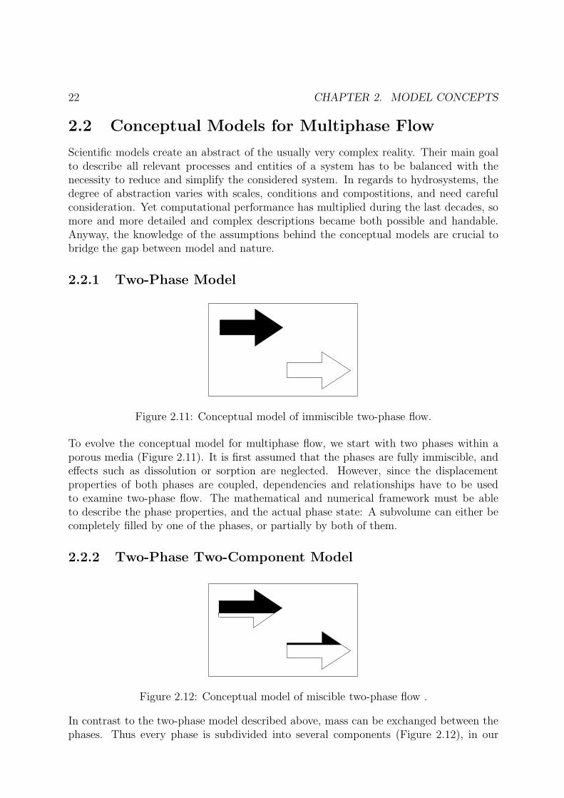
Figure 2.11: Conceptual model of immiscible two-phase flow.
To evolve the conceptual model for multiphase flow, we start with two phases within aporous media (Figure 2.11). It is first assumed that the phases are fully immiscible, andeffects such as dissolution or sorption are neglected. However, since the displacementproperties of both phases are coupled, dependencies and relationships have to be usedto examine two-phase flow. The mathematical and numerical framework must be ableto describe the phase properties, and the actual phase state: A subvolume can either becompletely filled by one of the phases, or partially by both of them.
2.2.2 Two-Phase Two-Component Model
Figure 2.12: Conceptual model of miscible two-phase flow .
In contrast to the two-phase model described above, mass can be exchanged between thephases. Thus every phase is subdivided into several components (Figure 2.12), in our

2.2. CONCEPTUAL MODELS FOR MULTIPHASE FLOW 23
case each phase consists of two components. Multicomponent models have to reproducethermodynamic mixing processes and thus the composition of the phases, as well astheir general spatial distribution and changes with time. However, proper kinetics ofthe mass exchange between the phases are most often ignored by assuming a reversibleprocess that run through a series of equilibrium states. The actual non-static processis approximated by a series of quasi-static states. This so-called local thermodynamic
equilibrium assumption may hold for slow processes which seem usual in porous media,but comes with the price of indispensable side-effects to account for non-static behaviourof real natural systems.
2.2.3 Shortcomings of the Discussed Approaches
As we have seen, the complex flow regime of multiphase flow and multicomponent trans-port is depicted by an extension of Darcy’s Law (see Chapter 2.1.3) with the help ofphase- or component-dependent constitutive relationships. This abstraction gives rise tothe following concerns:
a) Application of Darcy’s LawWhile the original empirical relationship was found examining singlephase flow throughhomogeneous porous medium, it is now used in its extended version for complex regimessuch as heterogeneous multiphase flow. The only conceptual change to the Darcy modelis an extension by the relative permeability and the adaption of the parameters to thevarying phase composition:
vα = −Kkrα
µα(∇pα − αg)
Thus the only driving forces for advective flows which are explicitly included are pressuredifferences and gravity. The relative permeability function has to account for all otherdriving forces, for example cross coupling of fluids (which means vn = vn(vw)) as wellas interfacial forces. As Hassanizadeh and Gray (1993) put it, the extension of Darcy’slaw to complex systems seems analogous to applying the ideal gas law to real gases byan increasingly complex ideal gas constant R, for example. They rather suggest to find ageneral formulation for real gases, that can in turn be simplified to the ideal gas law,
PV = nRT . (2.30)
Such an approach, the derivation of governing equations for multiphase flow which canthen be simplified to the extended Darcy method, will be presented in Chapter 2.3.
b) Macroscale CapillarityAs described in Chapter 2.1.2.1, capillarity on the microscale can be mathematicallydescribed using interface and fluid properties. On the REV-scale, however, standard ap-proaches use dependencies on volume-averaged properties such as saturation in place ofinterface-related parameters. This approach is not able to depict hysteresis: Capillarityon the macroscale is not only dependent on the state, but also on the process (wether thesoil is drained or imbibed) and the history of the soil (wether the soil is primarily drained

24 CHAPTER 2. MODEL CONCEPTS
Figure 2.13: Hysteresis of capillary pressure (Niessner and Hassanizadeh, 2009).
or drainage-imbibition cycles are regarded). Thus, capillary pressure varies between acertain range for a given saturation, as is shown in Figure 2.13.Additionally, several other inconsistencies are discussed in Hassanizadeh and Gray (1993).
As an example, capillary pressure is used to conjoin the averaged pressure of the phases,by using the supplementary constraint in equation (2.12). Whilst state equations for thephases predict a dependence on the density of the phases (i.e. pα = pα(, T )), usual cap-illary pressure functions solely regard the phase saturation as a parameter. Furthermore,let us consider a porous media in equilibrium, where both phases are subject to staticpressures. Thus equation (2.12) reduces to the form
pc = ng − wg , (2.31)
which means that the capillary pressure at equilibrium is independent from saturation,soil type or other properties. Thus the question arises wether a macroscale capillary pres-sure that is only dependent on saturation is a too simplified approach.
c) Relative PermeabilityAs already discussed, the relative permeability krα(Sw) is used to alter the single-phasepermeability in the presence of another phase. Although this parameter is not derivedfrom a physical upscaling process, this empirical scaling factor has to account for a com-bination of all coupling effects under multiphase conditions. In addition, the relativepermeability function is also hysteretic, and investigations indicate dependencies on a listof other parameters (Niessner and Hassanizadeh, 2009). Avraam and Payatakes (1995)summarize that relative permeability is also dependent on the capillary number, the vis-cosity ratio, wettablity characteristics expressed by the equilibrium contact angle θ, acoalescence factor, and discovered a strong correlation with the corresponding flow mech-anisms:
krα = krα(Sα; Ca, τ, cos θ, Co, saturation history, ...). (2.32)

2.3. THE NEW CONCEPT INCLUDING INTERFACIAL AREA 25
d) Mass TransferMass transfer between the phases can only take place across the fluid-fluid interface. How-ever, since the interfacial area is not known as a parameter, current model concepts makestrong assumptions regarding kinetic mass transfer. The approach discussed in Chapter2.2.2 uses the assumption of a local thermodynamic equilibrium, other methods are re-viewed in Niessner and Hassanizadeh (2008b). However, although the interfacial area isobviously important to examine fluxes over the interface, none of those approaches usesinterfacial area as a parameter. Thus, no physically motivated description of kinetic massexchange is possible.
2.3 The new Concept including Interfacial Area
Figure 2.14: Conceptual model of miscible two-phase flow with proper kinetic mass trans-fer.
To overcome the shortcomings of the standard models, Hassanizadeh and Gray (1980,1990, 1993) proposed a fundamental approach based on physical principles instead ofextensions to an empirical correlation. The concept provides equations that accountfor traditionally inaccessible phenomena, but can still be reduced to Darcy’s Law andstandard approaches which prove to be particularly stable for slow processes, for example.The changes of the conceptual model with regards to the standard models are as follows:
• The parameter held responsible for hysteretic behaviour of multiphase flow, the cap-illary pressure, is not solely calculated from static experimental curves. Instead, ageneral constitutive correlation including all the relevant macroscale material prop-erties is employed. An additional balance of specific interfacial area yields for thephenomena of capillarity as an macroscale primary variable.
• The interfaces between the phases are also taken into account. This includes bal-ancing at the interface, as well as considering the total area of the interface as avariable determining the processes. Note that the interface between the solid matrixand the fluids is not included in this work, so sorptive effects are neglected.

26 CHAPTER 2. MODEL CONCEPTS
• A thermodynamic equilibrium is not presumed, so the new approach is not limitedto problems where this assumption holds. Moreover, it is expected that simulationsbetter approximate the natural behaviour of non-equilibrium if thermodynamic con-siderations are fully included.
The changes to the standard approach can be best described following the mathematicaldevelopment of the governing equations, which is done in Chapter 3.3.
2.3.1 Constitutive Relationships
By extending general balances, new relationships arise for the new concept. Followingthe principal idea behind the work of Hassanizadeh and Grey, the new correlationsare physically motivated and solely based on primary variables. They are meant to rep-resent the complex behaviour of two-phase flow, without the need for artificial fitting orcorrelation parameters.
2.3.1.1 Relative Permeability krα
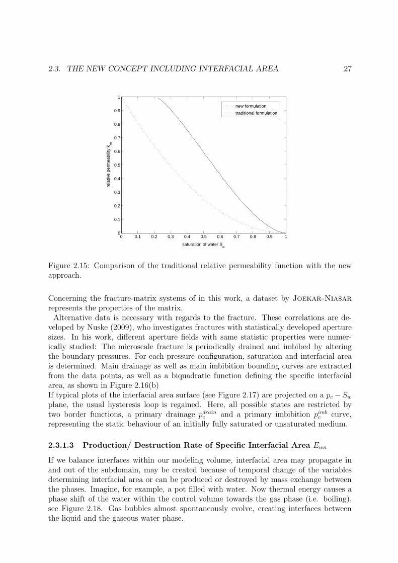
Through exploitation of thermodynamic principles, Hassanizadeh and Gray (1993) de-rived equations of motion, which directly lead to expressions for the phase velocities. Incomparison with the multiphase formulation of Darcy’s law, additional dependenciesbesides the pressure gradient and gravity are observable, while the artificial parameter ofthe relative permeability reduces to the saturation squared. The coefficients defining theseadditional terms, however, are only dependent on the saturation and specific interfacialarea (besides density and temperature, in the general case). This leads to the conjecturethat a comprehension of interfacial area redundantizes complex functions of the relativepermeability (Equations (2.19)). Instead, the factor S2
α = krα is used, which is displayedin comparison with the traditional function in Figure 2.15.
2.3.1.2 Specific Interfacial Area awn
Usually, the macroscale capillary pressure is derived from external curves originatingfrom equilibrium experiments, which face problems under dynamic conditions. Substan-tial derivation of thermodynamics (Hassanizadeh and Gray, 1993) as well as pore networkmodels (Joekar-Niasar et al., 2007) show that macroscale capillarity depends on the satu-ration and on the specific interfacial area awn, i.e. the interfacial area per representary ele-mentary volume. Being of biquadratic nature, this new functional relationship pc(Sw, awn)does not have to be unique for all given saturations and interfacial area (Fig 2.16(a)). Theinverse relationship, in contrast, is able to assign capillary pressure and saturation to aspecific interfacial area function, awn(Sw, pc) which is single valued. Joekar-Niasar et al.(2007) generated the data points for porous media computationally using pore-networkmodels, and obtained workable correlations by fitting bi-quadratic functions to the readingpoints with the coefficients
awn(Sw, pc) = a00 + a10 · Sw + a01 · pc + a11 · pc · Sw + a20 · S2w + a21 · p
2c . (2.33)
2.3. THE NEW CONCEPT INCLUDING INTERFACIAL AREA 27
0 0.1 0.2 0.3 0.4 0.5 0.6 0.7 0.8 0.9 10
0.1
0.2
0.3
0.4
0.5
0.6
0.7
0.8
0.9
1
saturation of water Sw
rela
tive
perm
eabi
lity
k rn
new formulation
traditional formulation
Figure 2.15: Comparison of the traditional relative permeability function with the newapproach.
Concerning the fracture-matrix systems of in this work, a dataset by Joekar-Niasar
represents the properties of the matrix.Alternative data is necessary with regards to the fracture. These correlations are de-
veloped by Nuske (2009), who investigates fractures with statistically developed aperturesizes. In his work, different aperture fields with same statistic properties were numer-ically studied: The microscale fracture is periodically drained and imbibed by alteringthe boundary pressures. For each pressure configuration, saturation and interfacial areais determined. Main drainage as well as main imbibition bounding curves are extractedfrom the data points, as well as a biquadratic function defining the specific interfacialarea, as shown in Figure 2.16(b)If typical plots of the interfacial area surface (see Figure 2.17) are projected on a pc − Sw
plane, the usual hysteresis loop is regained. Here, all possible states are restricted bytwo border functions, a primary drainage pdrain
c and a primary imbibition pimbc curve,
representing the static behaviour of an initially fully saturated or unsaturated medium.
2.3.1.3 Production/ Destruction Rate of Specific Interfacial Area Ewn
If we balance interfaces within our modeling volume, interfacial area may propagate inand out of the subdomain, may be created because of temporal change of the variablesdetermining interfacial area or can be produced or destroyed by mass exchange betweenthe phases. Imagine, for example, a pot filled with water. Now thermal energy causes aphase shift of the water within the control volume towards the gas phase (i.e. boiling),see Figure 2.18. Gas bubbles almost spontaneously evolve, creating interfaces betweenthe liquid and the gaseous water phase.

28 CHAPTER 2. MODEL CONCEPTS
(a) Interfacial area surface for the soil matrix (Joekar-Niasar et al., 2007).
(b) Interfacial area surface for the fracture (Nuske, 2009).
Figure 2.16: Interfacial area surfaces.

2.3. THE NEW CONCEPT INCLUDING INTERFACIAL AREA 29
Figure 2.17: Specific interfacial area of the fracture and corresponding bounding curves(Nuske, 2009).
Obviously, these production or destruction rates, denoted as Ewn in the following, arecrucial to any balance of interfaces. At this point, there are no experimental data availableconcerning this rate, thus Niessner and Hassanizadeh (2008a) proposed the following:A porous medium which is fully saturated with one phase does not possess any fluidinterfaces, thus awn = 0. As soon as the other phase infiltrates, interfaces are created.This production is increased the faster the phase gets removed (i.e. the faster the changein the phase saturation), hence Ewn ∝
(
∂Sw
∂t
)
. At some point during the invasion process,production of interfacial area must cease, and is to be reverted because at the end of thedisplacement process, one-phase conditions recur, i.e. awn = 0. So throughout a completedisplacement process, the rate of change of interfacial area Ewn > 0 (awn = 0) starts witha positive value, reaches a ridge value of awn ( with Ewn = 0) and settles down towardsawn = 0 with a negative value Ewn < 0. Following this characteristic, a further parametercharacterizing the magnitude of change as well as differencing between production anddestruction rate becomes necessary. Being separated from changes in the saturation, it iscalled the static part of the production rate, ewn which is derived in the following.
2.3.1.4 Static Production Rate of Specific Interfacial Area ewn
In the absence of experimental data, a formulation of ewn is gained mathematically by an-alyzing equation (3.34e). We assume that advective fluxes of interfaces play a minor partfor the distinction between production and destruction. Reformulation of the simplified

30 CHAPTER 2. MODEL CONCEPTS
awn = 0 awn > 0
⇒
ControlVolume
Heating
Pot
Figure 2.18: Production of Interfacial Area.
balance equation thus yields:
ewn(Sw, pc) ·∂Sw
∂t=
∂awn
∂t(2.34)
ewn(Sw, pc) =∂awn
∂pc·
((
dpc
dSw
))
process
+∂awn
∂Sw, (2.35)
where(
dpc
dSw
)
processstands for the the derivative of the actual path along the drainage
or imbibition cycle, whereas all other derivatives can be calculated analytically using the
general interfacial area function awn(Sw, pc) (Chapter 2.3.1.2). As long as(
dpc
dSw
)
processcan
not be deduced otherwise, Niessner and Hassanizadeh (2008a) propose to interpolate theproduction rate of the process path of interest between the two bounding solutions of theprimary drainage and primary imbibition process (see Figure 2.19(a)). Within the wide
0 0
ewn
edrainwn
eimbwn
S⋆w Sdrain
wSimbw
Sw
(a) Interpolation of ewn afterNiessner and Hassanizadeh (2008a).
0 0
ewn
edrainwn
eimbwn
p⋆c pdrain
cpimbc
pc
(b) More stable Interpolation of ewn .
Figure 2.19: Interpolation of the static production term of interfacial area.
range of possible saturations modeled in this work, numerical problems arise in areas with

2.3. THE NEW CONCEPT INCLUDING INTERFACIAL AREA 31
steep derivatives of the Van Genuchten-bounding curves. These occur in areas nearthe residual saturations Sw,res and Sn,res. An interpolation via saturation implies that allvalues Sw, Sdrain
w , Simbw may lie near residual, each producing steep slopes, and leads thus
to a predominance of the term(
dpc
dSw
)
process. It is hence supposed to interpolate known
ewn-values over capillary pressure, as shown in Figure 2.19(b), because then only the realsaturation Sw may lie within the range of the residual saturations. The correct staticproduction or destruction rate is thus interpolated between edrain
wn and eimbwn according to
ewn =1
(pdrainc − pimb
c )
(
edrainwn ·
(
pc − pimbc
)
+ eimbwn ·
(
pdrainc − pc
))
(2.36)

32 CHAPTER 2. MODEL CONCEPTS

Chapter 3
Mathematical and Numerical Model
3.1 Balance Equations for Two-Phase-Flow - 2p
control volume
solid matrix
non-wetting phase (n)
wetting phase (w)
In Iw
Aw
An
Qn
Qw
Mw
Mn
Figure 3.1: Mass balance of a control volume.
In general, multiphase flow can be described by balance equations for mass, momentumand energy (Helmig, 1997). Figure 3.1 shows a control volume with a solid phase and twofluid phases. To briefly derive a mass balance, we first consider a change of mass withinthe system over time, which yields a storage term denoted by M . Mass may furthermorebe transported over the boundary, referred to as the flux term A. Sources or sinks withinthe control volume are denoted by Q. Because we disregard mass exchange between thephases and the solid matrix, mass exchange I can only occur over the interface betweenthe phases. In the need of mass conservation, the mass balance can be formulated for allphases α:
Mα + Aα = Iα + Qα (3.1)
Fluid phases within the control volume Ω comprise the mass∫
Ω
SααdΩ. However, the
phases occupy only the available pore space φ, so the storage term Mα can be formulated
33

34 CHAPTER 3. MATHEMATICAL AND NUMERICAL MODEL
as follows:
Mα :=∂
∂t
∫
Ω
φSααdΩ (3.2)
We get the flux term Aα over Ω by applying the Gauss integral theorem yielding theflows over the boundary Γ:
Aα :=
∫
Ω
∇ · (φαvα)dΩ (3.3)
In multiphase models without components, exchange between the phases is neglected,because the phases are expected to be immiscible:
Iα :=
∫
Ω
iαdΩ = 0 (3.4)
Production or withdrawal due to external sources or sinks is given as follows:
Qα :=
∫
Ω
qαdΩ (3.5)
Inserting the terms (3.2), (3.3), (3.4) and (3.5) into equation (3.1) gives:
∂
∂t
∫
Ω
φSααdΩ +
∫
Ω
∇ · (φαvα)dΩ =
∫
Ω
qαdΩ (3.6)
Equation (3.6) can also be written in differential form as
∂(φSαα)
∂t+ ∇ · (φαvα) = qα . (3.7)
Generally, the term vα has to be expressed by a solution of the Naiver-Stokes equation,which describes the flow on the pore scale. However, within the concept of an REV,Darcy’s law may be used as a macroscale momentum equation.Replacing vα with equation (2.21b), equation (3.7) results in:
∂(φSαα)
∂t−∇
(
αkrα
µαK(∇pα − αg)
)
= qα (3.8)
With the additional constraints pn = pw + pc and Sn + Sw = 1, the unknowns for whichthe equation system has to be resolved are reduced to one saturation and one pressure,therefore two mass balance equations are sufficient to close the system. As was discussedin Chapter 2.1.1.4, porosity is kept constant, and may be thus excluded from the partialexpression of the storage term. We thus conclude for both phases
φ∂(wSw)
∂t−∇ ·
(
wkrw
µwK(∇pw − wg)
)
= qw , (3.9a)
φ∂(nSn)
∂t−∇ ·
(
nkrn
µnK(∇pn − ng)
)
= qn . (3.9b)

3.2. BALANCE EQUATIONS FOR COMPONENTS - 2P2C 35
A resume of the dominant underlying assumptions of equations (3.9) includes
• No mixture or solution of the two fluid phases.
• Mass transfer between fluids and solid disregarded.
• Porosity is kept constant.
• Velocity of the phases is resolved by Darcy’s law.
• Dispersion is not taken into account.
3.2 Balance Equations for Components - 2p2c
If the solubility among the phases cannot be neglected, an expression for the componentsκ has to be implemented into the pure twophase balance equation (3.1):
Mκα + Aκ
α = Iκα + Qκ
α (3.10)
The single terms are set up as for the 2p-model, but extended by mass fractions Xκα.
Hence the number of unknowns in a twophase two-component system is enhanced byadditional mass fractions. However, the corresponding mass fractions can be calculatedwith the additional supplementary constraint
∑
κ
Xκα = 1. In order to set up the mass bal-
ance, we have to balance all components in the respective phases. For a twophase systemconsisting of two components, this yields four balance equations. If there are solubilityeffects, for example, mass is transferred over the interface, and the mass exchange Iκ
α
cannot be neglected. Several means to determine mass exchange are discussed in Helmig(1997); Niessner and Hassanizadeh (2008b)Most standard models assume that the time scale of mass transfer is large comparedto the time scale of flow, which means that the composition of the phases is at a localthermodynamic equilibrium. Mass fractions are therefore directly calculated with ther-modynamic laws for equilibrium states, which is discussed in Chapter 2.1.4.2, justifiedby considerably low solubility limits. This equilibrium assumption reduces the unknownstate variables to two, thus a reduction to two equations is possible. The total mass ofa component is balanced by a summation over equal components, which eliminates themass exchange terms Iκ
α. To enhance readability, components A, W and phases w, n areused instead of general expressions:
W : φ∂(
¯wSwXWw + ¯nSnX
Wn
)
∂t−∇ ·
(
¯wXWw vw + ¯nXW
n vn
)
−∇ ·(
jWw + jWn)
= qw
(3.11a)
A : φ∂(
¯wSwXAw + ¯nSnX
An
)
∂t−∇ ·
(
¯wXAw vw + ¯nXA
n vn
)
−∇ ·(
jAw + jAn)
= qn
(3.11b)

36 CHAPTER 3. MATHEMATICAL AND NUMERICAL MODEL
with
vw = −K ·krw
µw(∇pw − ¯wg) (3.12)
vn = −K ·krn
µn(∇pn − ¯ng) (3.13)
pc = pn − pw (3.14)
Sw + Sn = 1 (3.15)
XWw + XA
w = 1 (3.16)
XWn + XA
n = 1 . (3.17)
(3.18)
Note that the mass balance contains macroscale diffusion jκα within the flux term Aκα,
which can be calculated by a Fick‘ian diffusion expression:
jκα = −Dκαα∇Xκ
α, (3.19)
where Dκα are macro-scale diffusion coefficients. On the macroscale, structural properties
of porous media are described by the tortuosity, which accounts for the elongation ofthe path lengths due to convolutions, and porosity. Microscale diffusion coefficients Dκ
α
which can be found in the literature, are thus upscaled with dependencies on saturation,porosity and tortuosity (Helmig, 1997):
Dκα = φτSnD
κα . (3.20)
Here, Dκα is the real, microscale diffusion coefficient (see Atkins and De Paula (2006);
Cussler (1997)) and the tortuosity τ can be gained, for example, through the model ofMillington and Quirk (1961):
τ = φ1
3 S7
3
n . (3.21)
To conclude the most important assumptions of equations (3.11):
• Solution and phase mixtures are treated by equilibrium laws (see Chapter 2.1.4.2).
• Mass transfer between fluids and solid disregarded.
• Porosity is kept constant.
• Velocity of the phases is resolved by Darcy’s law.
• Dispersion is not taken into account.
• Diffusion is resolved by an Fick-ian expression.

3.3. BALANCE EQUATIONS INCLUDING INTERFACIAL AREA - 2P2CIA 37
3.3 Balance Equations including Interfacial Area -
2p2cia
3.3.1 Mass and Momentum Equations
To introduce the new approach including interfacial area, the derivation of the basicbalance equations is discussed in more detail than the standard approaches in the previouschapters. In a two-phase system, both phases and the fluid-fluid interface can be balancedwith six mass and three momentum balance equations.1a) Mass balances for phase components (here for κ · α = 4 equations):
Phase w:∂(
φSw ¯wXκw
)
∂t+ ∇ ·
(
φSw ¯wXκwvw
)
−∇ ·(
φSw jκw)
= ¯wQκw +
1
V
∫
Awn
[wXκw (vwn − vw) + jκw] · nwn dA (3.22)
Phase n:∂(
φSn ¯nXκn
)
∂t+ ∇ ·
(
φSn ¯nXκn vn
)
−∇ ·(
φSnjκn
)
= ¯nQκn +
1
V
∫
Awn
[nXκn (vwn − vn) + jκn] · nwn dA (3.23)
1b) Momentum balance for phases (2):
Phase w:∂ (φSw ¯wvw)
∂t+ ∇ · (φSw ¯wvwvw) −∇ · (φSwTκ
w)
=1
V
∫
Awn
[wvw (vwn − vw) + tκw] · nwn dA (3.24)
Phase n:∂ (φSn ¯nvn)
∂t+ ∇ · (φSn ¯nvnvn) −∇ · (φSnT
κn)
=1
V
∫
Awn
[nvn (vwn − vn) + tκn] · nwn dA (3.25)
2a) Mass balances for wn-interface components (2):
∂(
ΓwnXκwnawn
)
∂t+ ∇ ·
(
ΓwnXκwnawnvwn
)
−∇ ·(
jκwnawn
)
=1
V
∫
Awn
[wXκw (vw − vwn) + jκw + nXκ
n (vn − vwn) + jκn] · nwn dA (3.26)
2b) Momentum balance for wn-interface (1):
∂(
Γwnvwnawn
)
∂t+ ∇ ·
(
Γwnvwnawnvwn
)
−∇ · (Tκwnawn)
=1
V
∫
Awn
[wvw (vw − vwn) + tκwn + nvn (vn − vwn) + tn] · nwn dA, (3.27)

38 CHAPTER 3. MATHEMATICAL AND NUMERICAL MODEL
where the overbars denote volume-averaged (macro-scale quantities). Besides, Awn is theinterface separating the w-phase and the n-phase in an averaging volume, Γwn is the arealmass density of the wn-interface, and jκwn is the diffusive flux of component κ in thewn-interface. A solution of a system of 9 coupled differential equations requires decentamount of computational power, plus constitutive relationships that are currently notavailable. Therefore Niessner and Hassanizadeh (2008b) proposed a simplified version,which can be seen as a extension of the equation system presented in Chapter 3.2 to asystem of five partial differential equations, which include specific interfacial area as aparameter.
3.3.1.1 Balances for Bulk Phases
In analogy to the typical models of multiphase flow, the momentum balances for the bulkphases are simplified to Darcy-equations, which can then substituted the expressions forthe velocities vα on the left hand side in equations (3.22) and (3.23). We then analyzethe right hand side representing mass exchange between the phases and interfaces byseparating the advective (Iκ
adv,α) and the diffusive (Iκdiff,α) mass transfer:
∂(
φSα ¯αXκα
)
∂t+ ∇ ·
[
φSα ¯αXκα (−K · λw (∇pα − ¯αg))] −∇ ·
(
φSαjκα
)
=¯αQκα +
1
V
∫
Awn
[αXκα (vwn − vα) + jκα] · nwn dA
=¯αQκα + Iκ
adv,α + Iκdiff,α (3.28)
Niessner and Hassanizadeh (2008b) argue that the advective transfer of mass over theinterface does barely influence the total mass of the bulk phase, so the term Iκ
adv,α forthe bulk phases is negligible. For the interfaces in contrast, advective transfer resultsin a production (or respectively destruction) term denoted as Ewn. The diffusive masstransfer term Iκ
diff,α represents a microscale behaviour, and Niessner and Hassanizadeh(2008b) obtained a first-order Fick’ian expression:
Iκdiff,α = jκα · nwn = ±
Dκ ¯α
dκawn
(
Xκα,s − Xκ
α
)
(3.29)
with Dκ as the micro-scale Fick’ian diffusion coefficient for component κ, dκ as thediffusion length of component κ. Xα,s is the mass fraction corresponding to the solubilitylimit of component κ, and Xα is the real mass fraction at a distance of dκ from theinterface.Note that in contrast to the diffusive fluxes discussed around equation (3.19), this diffusiveprocess is described by microscale quantities. Thus, it is hard to quantify a correctdiffusion length dκ corresponding to the modeled problem.
3.3.1.2 Balances for the Interfaces
In their work, Hassanizadeh and Gray (1993) summarized their combination of the massand momentum balances, plus energy and entropy balances using the second law of ther-modynamics. Analogous to their derivation from momentum balances of phases to the

3.3. BALANCE EQUATIONS INCLUDING INTERFACIAL AREA - 2P2CIA 39
Darcy equation, they reduced the general momentum balance of the interface. On themacroscopic scale, inertial and viscous effects are neglected in the momentum balance ofthe interfaces, as it is done with the fluids. An exploitation of the entropy balance in com-bination with the second law of thermodynamics yields a simplified and linearized formof the momentum balance of the interface (Hassanizadeh and Gray, 1990). According tothe procedure of phases, cross-coupling effects of viscous drag forces are neglected, whichleads to the following equation of motion:
Rwn · vwn = ∇(awnγwn) − awnΓwng − awnΓwnΛwn∇Sw , (3.30)
with the material properties Rwn and Λwn, velocity of the wn-interface (i.e. the interfacebetween the fluid phases) vwn, the macro-scale surface tension γwn, and the interfacialmass density Γwn. If we now state that the effect of gravity on the interfacial movement isnegligible, which is reasonable since we disregard any surfactants that possibly increase themass of the interface significantly, the term awnΓwng gets zero. Until further investigationsare undertaken about the influence of the last term in equation (3.30), we assume thatthe only driving force for interfacial movement is a gradient of specific interfacial area∇awn. With these assumptions, equation (3.30) can be simplified for two phases to
vwn = −Kwn∇awn , (3.31)
where Kwn is a new material property which combines the resistance R−1wn to interfacial
movement originating from drag forces and the influence of surface tension γwn. We thusend up with a Darcy-like expression for interfacial area movement, analogous to the bulkphases.
Focusing on the mass conservation, we assume that no surfactants are involved, so fluxesthrough the interface do not affect the compostition of the interface. This yields that allthe mass propagating from one phase into the interface has to end up in the other phase,or leads to an increase or decrease of interfacial area. The mass balance in equation (3.26)can therefore be summed up to one total mass balance of all components in the interfacewith
∑
κ
Xκwn = 1, eliminating mass fractions:
∂ (awn)
∂t+ ∇ · (awnvwn)
=1
V · Γwn
∫
Awn
[
w (vw − vwn) + (jAw + jWw ) + n (vn − vwn) + (jAn + jWn )]
· nwn dA
=1
V · Γwn
∫
Awn
[w (vw − vwn) + n (vn − vwn)] · nwn dA (3.32)
Note that all diffusive terms jκα on the left hand side vanish after the summation be-cause any loss of matter in one phase has to be fully replaced by the other component, i.e. jWw = −jAw. The appropriate consideration also holds for the microscale diffusivefluxes on the right hand side, but since it represents inter-phase transfer, mass is replacedfrom the respective phase, i.e jWw = −jAn . It is not reasonable to neglect the advec-tive mass transfer for interfaces as it was done for the bulk phases (3.3.1.1), therefore
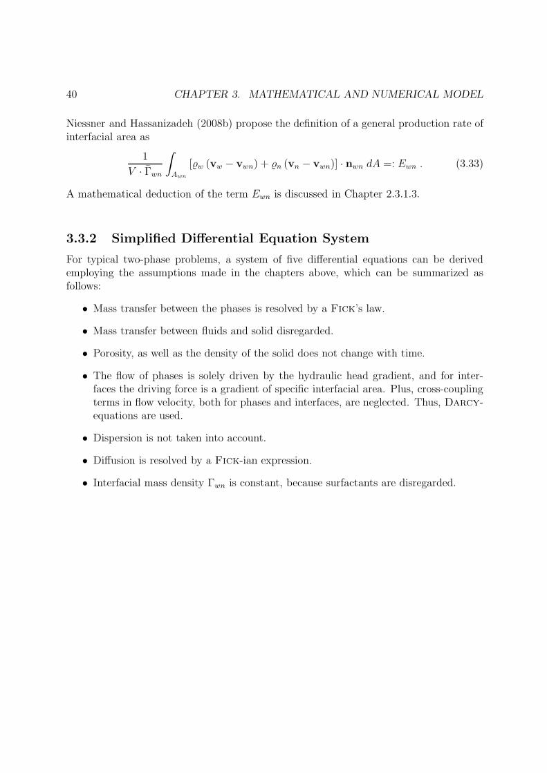
40 CHAPTER 3. MATHEMATICAL AND NUMERICAL MODEL
Niessner and Hassanizadeh (2008b) propose the definition of a general production rate ofinterfacial area as
1
V · Γwn
∫
Awn
[w (vw − vwn) + n (vn − vwn)] · nwn dA =: Ewn . (3.33)
A mathematical deduction of the term Ewn is discussed in Chapter 2.3.1.3.
3.3.2 Simplified Differential Equation System
For typical two-phase problems, a system of five differential equations can be derivedemploying the assumptions made in the chapters above, which can be summarized asfollows:
• Mass transfer between the phases is resolved by a Fick’s law.
• Mass transfer between fluids and solid disregarded.
• Porosity, as well as the density of the solid does not change with time.
• The flow of phases is solely driven by the hydraulic head gradient, and for inter-faces the driving force is a gradient of specific interfacial area. Plus, cross-couplingterms in flow velocity, both for phases and interfaces, are neglected. Thus, Darcy-equations are used.
• Dispersion is not taken into account.
• Diffusion is resolved by a Fick-ian expression.
• Interfacial mass density Γwn is constant, because surfactants are disregarded.

3.3. BALANCE EQUATIONS INCLUDING INTERFACIAL AREA - 2P2CIA 41
This leads to the final set of equations for the new approach:
φ∂(
Sw ¯wXWw
)
∂t+ ∇ ·
(
¯wXWw vw
)
−∇ ·(
jWw)
= ¯wQWw −
DW ¯n
dWawn
(
XWn,s − XW
n
)
(3.34a)
φ∂(
Sw ¯wXAw
)
∂t+ ∇ ·
(
¯wXAw vw
)
−∇ ·(
jAw)
= ¯wQAw +
DA ¯w
dAawn
(
XAw,s − XA
w
)
(3.34b)
φ∂(
Sn ¯nXWn
)
∂t+ ∇ ·
(
¯nXWn vn
)
−∇ ·(
jWn)
= ¯nQWn +
DW ¯n
dWawn
(
XWn,s − XW
n
)
(3.34c)
φ∂(
Sn ¯nXAn
)
∂t+ ∇ ·
(
¯nXAn vn
)
−∇ ·(
jAn)
= ¯nQAn −
DA ¯w
dAawn
(
XAw,s − XA
w
)
(3.34d)
∂awn
∂t+ ∇ · (awnvwn) = ewn(Sw, pc) ·
∂Sw
∂t= Ewn (3.34e)
vw = −K ·S2
w
µw(∇pw − ¯wg) (3.34f)
vn = −K ·S2
n
µn(∇pn − ¯ng) (3.34g)
vwn = −Kwn∇awn (3.34h)
pc = pn − pw (3.34i)
Sw + Sn = 1 (3.34j)
XWw + XA
w = 1 (3.34k)
XWn + XA
n = 1 (3.34l)
awn = awn(Sw, pc), (3.34m)
The macro-scale diffusive fluxes jκα are calculated according to the standard model byFick’s law, using equation (3.19) in combination with (3.20).In order to fully describe present and future states of a given system, a minimal numberof independent variables are needed, which are denoted as primary variables. All otherstate variables can then be obtained by constitutive relationships, as discussed in Chapter2.1.2. While the traditional approach uses constitutive relationships for mass fractionsand capillary pressure, the five balance equations in the new approach permit a solutionof five primary values:
• In analogy to the equation system described in Chapter 3.1 we also have a twophasesystem, so one saturation and one pressure are primary unknown variables (thecorresponding pressure and saturation are coupled by pn = pw+pc and Sn+Sw = 1).For further information, it is referred to the Gibbs phase rule in any thermodynamictext book.
• In contrast to the two-component model of Chapter 3.2 we do not postulate equi-librium mass fractions, so two of the real mass fractions are also primary unknownvariables (closed by the supplementary constraint
∑
κ
Xκα = 1 for all phases α).

42 CHAPTER 3. MATHEMATICAL AND NUMERICAL MODEL
• A thermodynamically derived balance of interfacial area is able to deduce the cap-illary pressure as the fifth unknown variable from a dependancy of pc on awn andSw (i.e. pc = pc(awn, Sw)).
To find a unique solution for the partial differential equations, the set of primary variableshave to be initially defined to declare the starting state of the system, which are thuscalled initial values. Boundary conditions interrelate the equation system with its spatialsurroundings. The spatial boundary conditions mostly used are Dirichlet boundaryconditions uD along boundary ΓD, as well as Neumann boundary conditions uN alongboundary ΓN :
u = uD Dirichlet boundary condition (3.35a)
∂u
∂n= uN Neumann boundary condition (3.35b)
With respect to the general form of the balance equation, the Neumann boundary con-dition represents a flux across the boundary ΓN (see Chapter 3.4.2) with respect to theexterior unit normal vector n, denoted in this work with qN,α.

3.4. NUMERICAL DISCRETIZATION 43
3.4 Numerical Discretization
u
f(u)
t,x, · · ·
u1 u2
u3
Figure 3.2: Discretization ofany variable u.
All mathematical models described afore are based on a sys-tem of balance equations which are both highly coupled andnon-linear, where an analytical solution does not exist. Tosolve the differential equations numerically, a certain dis-cretization scheme is needed to approximate the functionsf(u) by discrete values u at certain spatial and temporalnodes corresponding to an underlying grid (see Figure 3.2).The finer the grid is chosen, the closer the numerical ap-proximation gets towards an accurate solution of the math-ematical problem, yet a fine grid obviously comes with theprice of high computational costs.As has been discussed in the mathematical models inthis chapter, all governing equations are based on time-dependent storage term M , a flux term A and sources orsinks I +Q (equations (3.1) and (3.10)). This allows to dis-cretize all three approaches likewise. However, in order toget towards a consistent discretization of the unknowns u,they are separated from the terms of equation (3.10) to get a matrix form of the equationsystem as in Helmig (1997)
M ·
[
du
dt
]
+ A · [u] = R , (3.36)
where R comprises the matrix of the Neumann boundary fluxes, as well as sources andsinks and mass transfer terms. This equation system in matrix form can then be solvedusing, for example, an iterative Newton method. The discretization of M := M(u) ·
[
dudt
]
in time will be done in Chapter 3.4.1, whereas the spatial discretization will be presentedin Chapter 3.4.2.
3.4.1 Time Discretization
In this diploma thesis, time dependent problems for the different model concepts aresolved by an implicit Euler-method (Helmig, 1997), by what timestep sizes are notgenerally restricted by stability. While the spatial discretization is conducted with anfinite element discretization, a finite difference scheme is applied to discretize in time.Thus the differential operator ∂
∂tis approximated by a difference quotient over the timestep
∆t.Reformulating (3.36) to separate the differential operator yields
[
du
dt
]
= M−1·
(
−A · [u] + R)
, (3.37)
which corresponds to an an differential equation of the form
du
dt= f(u) . (3.38)

44 CHAPTER 3. MATHEMATICAL AND NUMERICAL MODEL
The application of an implicit Euler integration will yield for timestep m and its suc-cessive timestep m + 1:
um+1 − um
∆t= f(um+1) (3.39a)
um+1 = um + ∆t · f(um+1) . (3.39b)
Thus, transferred back to equation (3.36), the discretization in time yields:
[
um+1]
= [um] + ∆t · M−1·
(
A · [u] + R)
(3.40)
It was tested if the static production term in equation (3.34e) has to be also discretizedfor both timesteps within the implicit Euler-step as
Em+1wn =
em+1wn Sm+1
w − emwnSm
w
∆t,
or directly calculated from the new timestep:
Em+1wn = em+1
wn
Swm+1
− Smw
∆t.
Because the latter reduces computational effort to only one static production rate em+1wn per
timestep, significant performance benefits can be gained without any noticeable effects onthe solution. Besides, this solution technique corresponds more to the physical meaningof a static production rate as a source or sink to the interfacial area balance.
3.4.2 Space Discretization
The spatial discretization scheme used in this thesis is a fully upwinding finite-elementfinite-volume method, or box-method (Helmig, 1997; Helmig and Huber, 1998). The wholemodel domain G is first covered by a finite-element mesh with the nodes at the cornersof the elements e. The correct analytical solutions f(u) = (f(Sw), f(pc), f(awn) · · · ) arethus approximated according to a finite-element approach by:
u ≈ u =∑
i
uiNi , (3.41)
where Ni prescribes an interpolation function (also called shape function, ansatz functionetc.) at the node i, connecting the node i with all neighboring nodes j. The order of theshape functions determines the order of approximation, i.e. how close the discretizationcomes near the original solution f(u). Usually, as was done in this work, linear shapefunctions were used (see Figure 3.3, part I), with the restriction
Ni(xl) = δil =
1 if l = i , which means that xl ∈ Bi
0 otherwise, i.e. l = j or xl /∈ Bi .(3.42)
However, this discretization (u → u) leads to a global residual or global defect ε, which

3.4. NUMERICAL DISCRETIZATION 45
u
x
f(u)
u1 u2
u3
Ni,1 Ni,2
ij1 j2
→
(a) Part I: Ansatz Functions Ni.
u
f(u)
x
u1 u2
u3
Ni,1 Ni,2
ij1 j2
Error ε
→
(b) Part II: Error ε.
u
f(u)
x
FV-box Bi
u1 u2
u3
Ni,1 Ni,2
ij1 j2
(c) Part III: Discretization u andFV-box Bi.
Figure 3.3: Box-method .
i
Bi
e
barycenter ofelement e
Figure 3.4: Box construction in two dimensions, after (Class, 2001).
we want to be as small as possible (see Figure 3.3, part II). In case of an exact solutionof the primary variables, ε has to become zero. Therefore a weighting function Wi isintroduced which minimizes the error within the domain G:
∫
G
Wiε!= 0 for all i . (3.43)
A second mesh is layered around each node i of the finite element mesh, with its cornersat the edge midpoints or the centres of gravity of adjected elements, respectively (Figure3.4. Hence every node is contained within a bounding box Bi, building a secondary finitevolume mesh (see Figure 3.3, Part III). The whole model domain G is subdivided intosmaller subdomains, represented by the boxes Bi. Following the purpose of the weightingfunctions, they must satisfy the condition
∑
i Wi = 1 for all boxes∑
i Bi over the modeldomain G. Thus, the defect can be regarded within each subdomain of the model domain,so from the physical perspective a local mass conservation is enforced for each subdomain:
∫
Bi
Wiε!= 0 . (3.44)
This local mass conservation is one of the major advantages of the box method, while itstill features the flexibility of Finite Element methods.

46 CHAPTER 3. MATHEMATICAL AND NUMERICAL MODEL
To visualize the discretization with one example of the governing equations, the represen-tative but clear balance equation (3.34e) is chosen (the discretization of the other balancescan be found in, for example, Class (2001)): Inserting equation (3.41) in combination withequation (3.42) into equation (3.34e)), with upwinding of specific interfacial area in theflux term, yields
∑
i
∂(awn,iNi)
∂t+ ∇ ·
(
∑
i
aupwwn,ijKwn∇ (awn,iNi)
)
−∑
i
Ewn,i = ε . (3.45)
Upwinding techniques where developed, for example, by S. K. Godunov in 1959, exam-ining shock fronts of advective problems. Over the decades upwinding schemes proved tobe very robust by reducing numerical oscillation and producing considerably steep shockprofiles (B.van Leer and P.Roe in Hassaini et al. (1997)). Generally, the schemes use thedirection of propagation in a flow field, i.e. the characteristic speed, for the computationof advective fluxes. A simple first-order upwinding scheme is used here, defined by
aupwwn,ij =
awn,i for awn,i ≥ awn,j
awn,j otherwise, for awn,i < awn,j .(3.46)
We use a box-method weighting (equation (3.44)) to diminish the residual within one boxBi:
∑
k
∫
Bi
WiNk∂(awn,k)
∂t+
∫
Bi
Wi ∇·
(
∑
k
aupwwn,ikKwn∇ (awn,kNk)
)
−
∫
Bi
WiEwn,i = 0 , (3.47)
k comprises the specific node i of box Bi and all neighboring nodes j. The integral termin the middle, which was referred to as the flux term A at the beginning of this chapter,is transferred using the Green-Gauss theorem:
A :=
∮
ΓBi
Wi
∑
k
aupwwn,ikKwn∇ (awn,kNk)nΓBi
dΓBi−
∫
Bi
∇Wi
∑
k
aupwwn,ikKwn∇ (awn,kNk) dBi
(3.48)For the box scheme, the weighting function is piecewise constant within the box
Wi =
1 if within Bi
0 otherwise ,(3.49)
which means that ∇Wi = 0. Thus, the right integral of equation (3.48) vanishes. Fordiscretized values u, it holds that
∇u = ∇
(
∑
k
uk · Nk
)
=∑
k 6=i
(uk − ui)∇Nk =∑
j
(uj − ui)∇Nj . (3.50)
For any given box we also post that∫
BiNidBi = Vi , which is the volume of the box Bi.
All this combined, the equation (3.47) is discretized for each node i as
∂(awn,i)
∂tVi + 1 ·
∑
j
(awn,j − awn,i) aupwwn,ji
∮
ΓBi/∈ΓN
Kwn∇Nj · nΓBidΓBi
− Vi · Ewn,i = qN,α ,
(3.51)

3.4. NUMERICAL DISCRETIZATION 47
where ΓN denotes a Neumann boundary, and qN,α denotes Neumann boundary fluxes ofphase α.
Combining the spatial with the temporal discretization (equations (3.51) and (3.39a))yields
am+1wn,i − am
wn,i
∆t·Vi+
∑
j
(
am+1wn,j − am+1
wn,i
)
aupw,m+1
wn,ji
∮
ΓBi/∈ΓN
Kwn∇Nj ·nΓBidΓBi
−Vi·Em+1wn,i = qm+1
N,α .
(3.52)The flux integral over the boundaries is time independent as long as the shape functions,the permeability as well as the finite element mesh remain constant with time. Since noadaptive methods are used in this work, this restriction holds.
3.4.3 Implementation in DUMUX
All numerical simulations of this thesis are carried out using the programming frame-work DUNE, the Distributed and Unied Numerics Environment. Using C++ techniques,DUNE is a modular toolbox for the solution of partial differential equations for grid-basedproblems. The framework consist of modules such as solvers, grids or discretization algo-rithms etc., forming a ready-to-use toolbox for more specialized applications.The additional module DuMux (Dune for Multi -phase, -physics, -component, -scaleFlow in Porous Media) has been developed by Flemisch et al. (2007) to provide a frame-work for efficient implementation of models for porous media flow problems. Thus themodel for fully coupled two-phase flow can be used and adapted for the standard approachmodels of Chapter 2.2.2, while a new module had to be developed and implemented forthe new approach. As DuMux is still in the stage of development, one of the majortasks during the thesis was to maintain the interfacial-area module during the process ofongoing structural improvements.

48 CHAPTER 3. MATHEMATICAL AND NUMERICAL MODEL

Chapter 4
Case Studies
A numerical test scenario for two-phase flow is assembled to investigate the differencesbetween the model approaches on a fundamental basis, and to test the performance of thenew approach. Since principle investigations are intended, simple model configurations intwo dimensions are chosen to avoid disruptive effects. All study setups are based on thetest setup presented in the work of Jakobs (2004). In contrast to his studies, an interfacecondition at the boundary between the fracture and the matrix is not yet implementedto this stage: A relationship of pc(Sw, awn) is much more complicated than the standardcase of pc(Sw). However, this will be an important field of further development, as willbe presented later.Despite of the underlying motivation discussed in Chapter 1.4, the purpose of the numer-ical test cases was to show the functionality of the model concepts in the scope of strongparameter heterogeneities between the fracture and the matrix, as well as to indicate thedifferences, strengths, or disadvantages of the mathematical models, instead of simulatinga proper nuclear storage site. Up to this work, only homogeneous macroscale domainswere modeled with the new concept.
4.1 Model Setups
The sketches of the case setups are displayed in Figure 4.1. Fully saturated gas is infil-trated into a water-filled domain of 8m times 10m. Impermeable boundary conditionsare defined on both sides and at the bottom, aside from the infiltration interval rangingfrom 3m to 5m. At the top of the model domain, a Dirichlet-boundary is chosen, seeChapter 4.1.2.4. Three different principal setups may be distinguished:
1. Homogeneous setup: The model domain only consists of matrix material, no frac-tures are implemented. It is thus possible to examine a homogenous flow regime,without disturbance from discontinuities caused by the fracture-matrix interaction(left part of Figure 4.1).
2. A setup with one fracture: Located in the middle of the simulation domain, itstretches from 1m above the infiltration zone straight upwards to an height of 8m,comprising a width of 10cm (see the right part of Figure 4.1). Although it is referred
49

50 CHAPTER 4. CASE STUDIES
to as “one fracture”, the area is intended to represent an active flow system ofconnected fractures, see Figure 2.4.
3. Several fractures: a further fracture is added to examine the spread of the non-wetting phase under different gravitational influence. In addition, validity and ap-plicability of the new concept are surveyed. Both multifracture model setups arebased on Figure 4.1 b), and the actual conformation is explained at the beginningof the respective chapters.
10 [m]
8 [m] 8 [m]
a) Homogeneous
qNqN
x
y
b) One fracture
Dirichlet BCDirichlet BC
Boundary Condition I: Dirichlet
BC II: impermeable
BC III:Neumann qN
BC IV: impermeable
Figure 4.1: Sketches of the applied model setups.
4.1.1 Grid Generation
The choice of the numerical grid was found to be an important task to gain stability ofthe simulation runs and to produce valid results. Around the infiltration zone, a finerresolution leads to an increase in the pressure gradients. Thus a lower infiltration rateor smaller timesteps are needed to attain numerical convergence, which obviously results

4.1. MODEL SETUPS 51
Figure 4.2: Simulation grid created with mesh generator ICEM CFD.
in longer simulation runtimes until the gaseous front reaches the fracture. Furthermore,especially around the top and bottom node of the fracture, discretization resolution in-fluences the numerical stability.First attempts were made with a homogeneous quadratic grid, but the stability of thesimulation runs appeared enhanceable by using the mesh generator ICEM CFD. That is,the mesh is refined in the areas of interest around the fractures. It became even moreimportant when constructing a more complex geometry (see Chapter 4.2.3). For the setupof 1 fracture, the applied mesh is exemplarily displayed in Figure 4.2.
4.1.2 Model Parameters
Besides spatial information about the model domain, physical properties have to be pro-vided. Since the investigations are of principal nature, there was neither experimentaldata for the specific setup nor an existing natural template for the examined case, thussoil parameters could be chosen freely.
4.1.2.1 Fluid Parameters
In the simulation runs, water represents the wetting phase. Although the motivationwould indicate to simulate a gaseous phase composed of mainly hydrogen, gas with thestandard composition of air was selected as the non-wetting phase, because the highermolar mass of air caused less numerical fragility. The fluid parameters were displayed inTable 4.1.

52 CHAPTER 4. CASE STUDIES
Table 4.1: Fluid properties of the wetting and non-wetting phase.
Phase Substance Density[
kgm3
]
Diffusion coefficient [m2
s]
Wetting phase Water 1000 2.2 · 10−9
Non-wetting phase Air Ideal gas 2.25 · 10−5
4.1.2.2 Soil and Fracture Parameters
As already mentioned, we were free to use any soil parameters. However, natural con-ditions call for harsh differences between fractures and matrix, thus high differences inpermeability of 4 orders of magnitude are chosen. In order to compare all model con-cepts, a soil matrix with known interfacial-area surfaces, as well as bounding curves forprimary drainage and imbibition are necessary, and appropriate data is found in the workof Joekar-Niasar et al. (2007). Both for primary drainage and primary imbibition, a Van
Table 4.2: Comparison of soil properties between fracture and matrix.
Porosity Φ Conductivity K [m2] Initial Saturation Entry pressure pd
Matrix 0.1 10−12 0.95 6009.50 PaFracture 0.3 10−8 0.95 1067.05 Pa
Genuchten formulation was used, see Table 4.4. However, to visualize the differencesbetween fracture and matrix, Table 4.2 also shows the corresponding entry pressures ofa Brooks-Corey description: The open voids of the fracture are much larger than thebiggest pores of the matrix, the non-wetting phase can thus enter the domain of thefracture with ease. Hence, infiltration processes into the fracture proceed at much lowerpressures than re-exfiltration into the matrix.Interfacial area parameters (see Table 4.3) are bound to the biquadratic fitting functionsof equation (2.33). The Van Genuchten model parameters from Table 4.4 correspondto equation (2.16).
Table 4.3: Interfacial Area Surface Coefficients.
Interfacial Area Surface Function
a00 [ 1
m] a01 [ 1
m] a10 [ 1
m·Pa] a11 [ 1
m·Pa] a20 [ 1
m] a21 [ 1
m·Pa2 ]
Matrix 688.886 4167.65 -0.185 -0.039 -4058.7 1.058 · 10−5
Fracture -73.35 391.95 0.0058 -0.0232 -301.3818 −2.569 · 10−8

4.1. MODEL SETUPS 53
Table 4.4: Boundary Curves.
Primary Drainage Primary Imbibition Residual Saturation
α m n α m n Sw,res Sn,res
Matrix 0.00014 0.853 8.818 0.00024 0.928 14.0 0.069 0.390Fracture 0.000446 0.694 3.268 0.000615 0.885 8.696 0.212 0.391
Programming measures are undertaken that the residual saturation of the wetting phaseis set to zero if the primary drainage curve is regarded. As the standard approach isbound on drainage-only, the imbibition curve could not be implemented in this model.
4.1.2.3 Model Concepts
Three different model approaches form the basis of the simulations:
1. A standard two-phase two-component model, abbreviated as 2p2c (Chapter 3.2).This model is bound to states of equilibrium and macroscale capillarity is calculatedby a Van Genuchten description for primary drainage.
2. The extended two-phase two-component model which includes non-equilibrium ki-netic mass transfer over the interfaces, denoted as 2p2cia4. This is a simplified ver-sion of the new interfacial-area based approach presented in Chapter 3.3.2, wherewe disregard hysteretic behaviour of the capillary pressure, thus capillarity is boundon the primary drainage curve. The governing equations of this approach are thefour equations (3.34a) to (3.34d).
3. A full interfacial area approach as discussed in Chapter 3.3.2, including the fullequation system (3.34). Because of the five equations that are used, this model isabbreviated in the following as 2p2cia5. The full approach is not restricted to statesof equilibrium, and macroscale capillary pressure is obtained from the model.
The motivation for the application of all three models was to use the standard approach2p2c and extend it step by step (2p2cia4, 2p2cia5 ). It is thus possible to examine sta-bility as well as performance, and compare the simulation results to discuss wether thedifferences are significant or not.The more complex the equation system gets, the more independent primary variables maybe resolved, see Table 4.5. Note that the standard approach switches the second primaryvariable (Sn) to a mass fraction if one phase disappears.
4.1.2.4 Initial and Boundary Conditions
The set of initial values (Table 4.6) has to be chosen according to the set of primaryvariables, or the quantity of differential equations, respectively.

54 CHAPTER 4. CASE STUDIES
Table 4.5: Set of primary variables.
Primary Variables
Standard Approach (2p2c) pw, Sn
Simplified Interfacial Area Approach (2p2cia4 ) pw, Sn, XAw , XW
n
Interfacial Area Approach (2p2cia5 ) pw, Sn, XAw , XW
n , pc
Boundary Conditions (Chapter 3.3.2) are denoted in Figure 4.1, where Dirichlet ischosen along the top side, and all other boundaries are of type Neumann with
qN,n(x, y) =
−0.005 m3
m2sif 3m ≦ x ≦ 5m
0 otherwise, which means a no-flow boundary.(4.1)
Simulation results prove that the solution is independent from the Dirichlet boundaryat the top, because its distance from the area of interest, mainly the area around the topcorner of the fracture, is large enough to negate the influence of the boundary condition.
Table 4.6: Initial Boundary Conditions, identical to applied Dirichlet Boundary Con-ditions.
Initial and Dirichlet values Model Concept
Pressure pw [Pa] 10200 + (10 − y) · 9810 2p2c, 2p2cia4, 2p2cia5
Saturation Sn [-] 0.05 2p2c, 2p2cia4, 2p2cia5
Mass Fraction XAw [-] pn
HAw
2p2c, 2p2cia4, 2p2cia5
Mass Fraction XWn [-] pw,sat
pn2p2cia4, 2p2cia5
Capillary Pressure pc [Pa] pc(Sw) (Equation (2.16)) 2p2cia5
4.2 Verification Study for the Conceptual Models
4.2.1 Homogeneous Setup - No Fracture
The homogeneous setup allows general validation and verification of the different modelconcepts, plus an estimation of the significance of the underlying physical processes. Inorder to investigate general conformity of the results, the propagation of the gaseous phaseis compared after a 100 second simulation run, as shown in Figure 4.3. The encountereddifferences are predominantly caused by the different relative permeability descriptions ofthe respective models, see Chapter 2.1.2.2 versus Chapter 2.3.1.1. However, if capillar-ity and mass transfer due to non-equilibrium effects are to be compared, a similar frontpropagation is favorable. For further comparative studies, the simple relative permability

4.2. VERIFICATION STUDY FOR THE CONCEPTUAL MODELS 55
formulation kr,α = S2α is thus also applied to the 2p2c-model, which then yields good
congruence (Picture 4.3(d)). The results for all model concepts using the relative perme-ability function of Chapter 2.1.2.2 are also in full agreement.If variables besides the saturation are compared, let them be capillary pressure or mass
(a) 2p2c - Sn. (b) 2p2cia4 - Sn.
(c) 2p2cia5 - Sn. (d) 2p2c with permeability of kr,α = Sα.
Figure 4.3: Comparison of the different model concepts for the homogeneous case.
fractions, the conformity is also approved. Figure 4.4 illustrates the 2p2c-model drawn bya solid black line, the 2p2cia4 -model by a grey but dashed line, and the 2p2cia5 -model bya dotted black line. All characteristics match very well over time, the new approaches areable to resolve comparable results when the same relative permeability function is usedfor all models. Capillary pressure, however, shows small variances: Figure 4.4(a) indicatesa short imbibition process at the beginning of the simulation, thus the whole process isnot purely drainage. The model domain is, for numerical reasons to get the 2p2c-methodto convergence, not fully saturated with water at the beginning, therefore an increasein water saturation remains possible. When entering the domain, the propagating gasfront pushes forward an evolving water front, creating a small imbibition zone ahead ofthe strong drainage area at the gaseous front. For the homogeneous setup, however, thisimbibition process is too weak to significantly reduce capillary pressure and thus to sub-stantially influence the overall process.Additionally, the assumption of an equilibrium process and thus negligible mass transfer
seems appropriate for the slow homogeneous case. The real mass fractions gained by the

56 CHAPTER 4. CASE STUDIES
(a) Capillary pressure pc . (b) Mass fraction of air in water-phase XAn .
Figure 4.4: Temporal characteristics at an exemplary node.
extended models (2p2cia4, 2p2cia5 ) are very close to the equilibrium mass fractions ofthe standard approach (Figure 4.4(b)). Although mass transfer due to non-equilibrium isrecognizeable in Figure 4.5(a), the variation from equilibrium mass fraction is marginal:the mass transfer term in Equation (3.29) includes a diffusion coefficient which is 5 magni-tudes larger than the one for the component air. Recognizeable effects of non-equilibriumare solely detectable for the component air (Figure 4.5(b)). Areas below equilibrium,indicated by a positive sign of the mass transfer, are only observable in the vicinity of theinfiltration zone.
Figure 4.6 shows the saturation of the non-wetting phase (grey) as well as the non-
(a) Mass transfer of water into gaseous phaseIWn [ kg
sm3 ].(b) Mass transfer of air into water phase IA
w [ kgsm3 ]
.
Figure 4.5: Mass transfer after 50 seconds.
equilibrium mass transfer of air into water IAw (black) along the first meter of infiltration,
marked by the white line on the right picture. An infiltration rate of qN = −0, 005 kgsm2 is
represented by a solid line, while the dotted line marks qN = −0, 007 kgsm2 and the dashed
line qN = −0, 01 kgsm2 . With increasing infiltration rates, the phase velocity is also meant
to increase to sustain the gas flow. In consequence, more mass gets transferred due to

4.2. VERIFICATION STUDY FOR THE CONCEPTUAL MODELS 57
Table 4.7: Computational expenses for a 100 second simulation run.
model concept timesteps computational time
2p2c 14 80 s2p2cia4 14 158 s2p2cia5 15 228 s
non-equilibrium near the infiltration area, hence the distance of obtained mass fractionsfrom equilibrium mass fractions also increases. For problems with high infiltration rateswhich may be observed near the wells of sites for subsurface storage of carbon dioxide,non-equilibrium effects may thus play a significant role.As expected, the solution of more nonlinear equations enhances the computational de-
Figure 4.6: Mass transfer with respect to infiltration rates (black, in [ kgsm3 ]) and saturation
of the gaseous phase (grey, in [-]) .
mand. Table 4.7 lists the time to complete the simulation of 100 seconds as well as thenecessary timesteps. Both new concept require much more Newton-iteration steps toreach convergence, which explains increased computational demand without an increasein timesteps.

58 CHAPTER 4. CASE STUDIES
4.2.2 Fracture-Matrix System with One Fracture
The next model setup under investigation is a fracture-matrix system with one singlevertical fracture, see Figure 4.1 b). As discussed in the previous chapter, the standardapproach is used with the simplified relative permeability function to gain comparableresults. The pictures in Figure 4.7 show the saturation of the gaseous phase at the begin-
(a) 2p2c - Sn after 3s. (b) 2p2cia5 - Sn after 3s.
Figure 4.7: Different model concepts at the beginning of the simulation..
ning of the simulation (after three seconds which equals three timesteps). Gravity causesthe initial gas volume inside the fracture to propagate upwards and accumulate at the topnode of the fracture. That is the saturation of gas is lower inside the fracture comparedto the matrix which is generally still subject to initial saturations of around Sn = 0.05.Thus gas infiltrates from all sides into the fracture, slightly lowering the gaseous contentaround the fracture. In accordance to the homogeneous simulations, all model descrip-tions draw a comparative phase propagation. At this early stage of the simulation, massfractions of the interfacial-area models are lower than equilibrium mass fractions in thelower and upper part of the the fracture, because the flow velocity is instantly very high.This effect is caused by an initial gas volume in the fracture that is driven upwards bygravity. Since that flow regime is dependent on the initial conditions and is not subjectto the infiltration process, these starting effects are not discussed here.Throughout the simulation, mass transfer of water is primarily caused by numerical fluc-tuations rather than real differences in mass fractions, because the diffusion coefficient isfive orders of magnitude larger compared to that of the component air. Thus, slightlyenhanced flow velocities due to worse grid elements, for example, may already cause con-siderable mass transfer without any significant change in mass fractions.In contrast, mass transfer of the component air due to states of non-equilibrium, as de-fined by equation (3.29), is further examined. Apart from starting effects, mass fractions

4.2. VERIFICATION STUDY FOR THE CONCEPTUAL MODELS 59
of air below equilibrium (and thus positive mass transfer) are only observable at the infil-tration zone, which was already discussed for the homogeneous case, and is therefore notvisualized here. Figure 4.8 shows the mass transfer of air with a negative sign, i.e. transferof the component air into the non-wetting phase, at two representative timesteps. Apartfrom the infiltration front, negative mass transfer is encountered within the fracture assoon as it is flushed with gas (Figure 4.8(a)). The reason for this effect is ambiguous.One possible explanation may be numerical diffusion, which counteract .Later, as the upper side fills with gas, negative mass transfer is observable in the areas
(a) Mass transfer of air IAw after 24s. (b) Mass transfer of air IA
w after 60s.
Figure 4.8: Mass transfer of air IAw = DA ¯w
dA awn
(
XAw,s − XA
w
)
[ kgm2s
] .
where significant changes in saturation occur (Figure 4.8(b). Figure 4.9 compares realmass fraction XA
w (stroked) and equilibrium mass fraction XAw,s (dotted) for an exemplary
node in the upper area of the fracture with the wetting phase saturation Sw (dashed). Asthe gaseous plume spreads downwards, it reaches the selected node around 60 seconds,where even more water gets drained. These changes in saturation are too high to actuallyreach equilibrium. The final mass fraction of air in water can be found in Figure A.1 inthe appendix, as well as the final distribution of the non-wetting phase after 100 seconds.To investigate differences in capillary pressure, both approaches that are bound on pri-mary drainage (i.e. 2p2c and 2p2cia4 ) are compared with the 2p2cia5 -model featuringhysteresis. Figure 4.10 shows the chronological behaviour of the capillary pressure atthe bottom node of the fracture, drawn with respect to time (left) and to water satura-tion (right). The 2p2cia4 -model bound on the primary drainage process is representedby the solid black line. The other lines show instantiations of the 2p2cia5 -model withvarying permeability to the interfaces, ranging from Kwn = 10−10 [m3
s] (dotted, black),
Kwn = 10−11 [m3
s] (dashed, black) to Kwn = 10−12 [m3
s] (solid, grey). Within the first
six seconds, the 2p2cia5 -model is able to simulate the imbibition process of the fracture
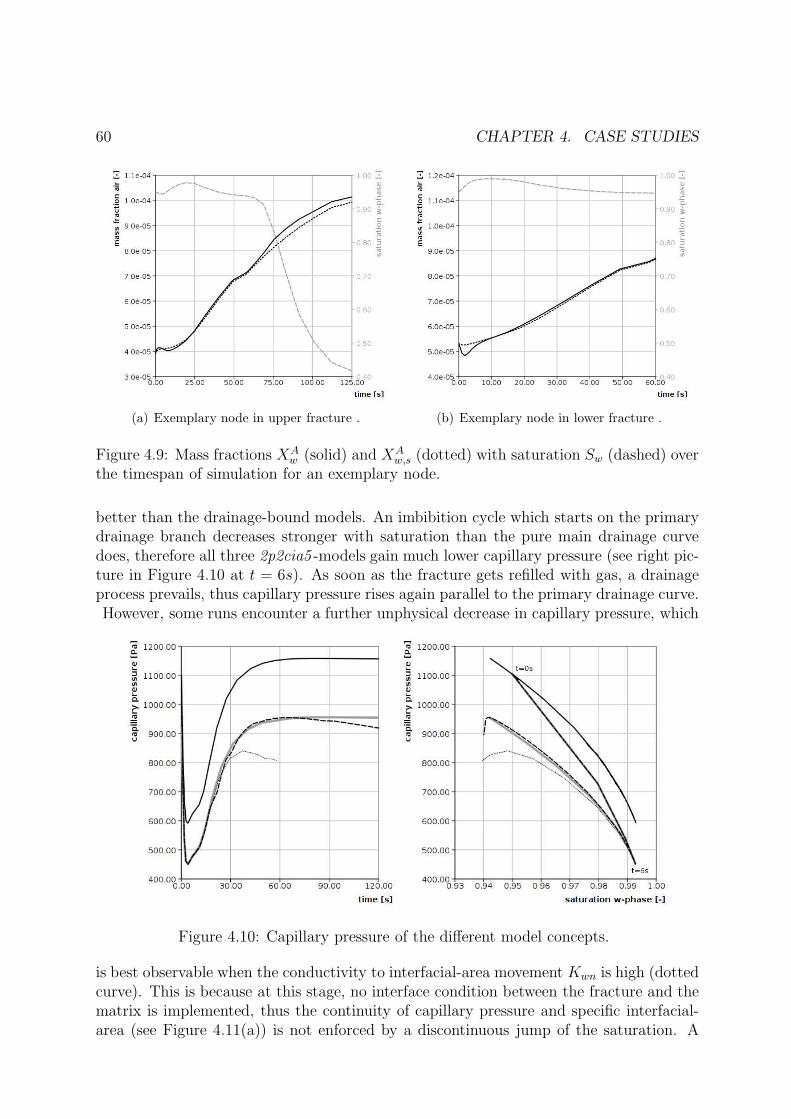
60 CHAPTER 4. CASE STUDIES
(a) Exemplary node in upper fracture . (b) Exemplary node in lower fracture .
Figure 4.9: Mass fractions XAw (solid) and XA
w,s (dotted) with saturation Sw (dashed) overthe timespan of simulation for an exemplary node.
better than the drainage-bound models. An imbibition cycle which starts on the primarydrainage branch decreases stronger with saturation than the pure main drainage curvedoes, therefore all three 2p2cia5 -models gain much lower capillary pressure (see right pic-ture in Figure 4.10 at t = 6s). As soon as the fracture gets refilled with gas, a drainageprocess prevails, thus capillary pressure rises again parallel to the primary drainage curve.However, some runs encounter a further unphysical decrease in capillary pressure, which
Figure 4.10: Capillary pressure of the different model concepts.
is best observable when the conductivity to interfacial-area movement Kwn is high (dottedcurve). This is because at this stage, no interface condition between the fracture and thematrix is implemented, thus the continuity of capillary pressure and specific interfacial-area (see Figure 4.11(a)) is not enforced by a discontinuous jump of the saturation. A

4.2. VERIFICATION STUDY FOR THE CONCEPTUAL MODELS 61
limit case of Kwn = 0 would result in equation (3.34e) being independent of the spatialvariation of specific interfacial-area. Thus, from the mathematical perspective, continuityof specific interfacial area does not have to be enforced. Therefore, the missing implemen-tation of an interface condition regarding to specific interfacial area is no more crucialto the solution. In our applied range of Kwn, interface conductivity with low magnitudepermits steep gradients, which produces less problems in regards to a missing interfacecondition. Higher interface conductivity results in greater fluxes evening out the gradients,therefore equation (3.34e) gets more dominated by diffusive fluxes, which necessitates thatthe continuity of the state variable has to be preserved.
Compared with the homogeneous case, the heterogeneous setup demands higher computa-tional efforts, thus all three model concepts require more time to finish the simulation, seeTable 4.8. Again, the different models concepts require comparable amount of timesteps,thus the computational effort has to be spent to reach convergence within each time step.Note that the performance of the 2p2cia5 -model varies with the parameter of interfacepermeability, Kwn.
Table 4.8: Computational expenses for the fractured case.
model concept timesteps computational time
2p2c 21 230 s2p2cia4 22 503 s2p2cia5 21 715 s
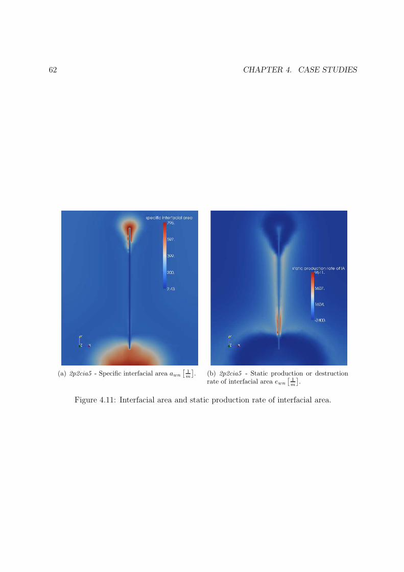
62 CHAPTER 4. CASE STUDIES
(a) 2p2cia5 - Specific interfacial area awn
[
1
m
]
. (b) 2p2cia5 - Static production or destructionrate of interfacial area ewn
[
1
m
]
.
Figure 4.11: Interfacial area and static production rate of interfacial area.

4.2. VERIFICATION STUDY FOR THE CONCEPTUAL MODELS 63
4.2.2.1 Simulatory Challenges for the Heterogeneous Setup
Figure 4.12: Saturation Sn at various nodes over the timespan of simulation.
For various periods, some models fail to converge because of distinct mechanisms, whichare addressed chronologically in this subchapter. To gain some orientation, an overviewof the temporal changes in saturation is given in Figure 4.12. The first numerical obstacleis formed after around six seconds, when the initial drainage process inside the fractureis reversed by an infiltration of gas from the matrix. Models with high conductivity tointerfacial movement fail to reverse the imbibition process (i.e. fail to reelevate saturationand thus capillary pressure) at the bottom corner of the fracture, and the simulationaborts. Such a failing simulation run with Kwn = 10−8 [m3
s] is visualized in Figure 4.13(a)
with a dotted black line, in comparison with successful simulations of Kwn = 10−12 [m3
s]
(grey solid) and the 2p2cia4 -model (black solid).At the beginning, capillary effects drained the areas around the fracture. Later, when
the fracture gets consistently filled with gas, exfiltration into matrix commences aroundthe upper part of the fracture because of gravitational forces. After reinfiltration into thematrix has started, another turning point in the characteristic of the saturation in theupper areas of the fracture indicates a further increase in the gaseous saturation, becausethere is still a consistent gas flow through the fracture: Around 24 seconds, the front of thegaseous phase reaches the fracture, which thus gets considerably filled with gas (Figure4.14(a)). While the fracture gets filled up even in the lower parts, the gaseous flow fromthe matrix into the fracture reverses. These turning points cause the sign of the term∂Sw
∂tto alter, which results in convergence problems concerning the fifth balance equation
over the Newton-steps: although it is a physically correct behaviour, it is challengingfor numerical stability. Some configurations of the 2p2cia5 -model with, for example, poormesh quality or again high permeability values for the interfaces Kwn, do not succeed inswitching the flow process at the adjected nodes to the fracture, and thus fail to converge

64 CHAPTER 4. CASE STUDIES
(a) Capillary pressure over the time at the bot-tom edge of the fracture.
(b) Production term of interfacial area in an up-per node neighboring to the fracture IA
w .
Figure 4.13: Numerical obstacles at 6seconds (left) and 30 seconds (right).
around 30 seconds.To improve convergence, especially for configurations with higher permeability to in-
terfacial area, it was necessary to limit the influence of the term ∂awn
∂pc·
(
dpc
dSw
)
processof
equation (2.35), because both factors can attain very high values. Models without sucha limitation procedure gain such overdominated static production terms that they stopany further charging of the fracture: The fracture then seems sealed after 20 seconds andsimulations abort before 40 seconds, without any change in the fracture saturation. Yetit is expected that deeper knowledge about the general production term Ewn, either byexperiments or by microscale simulatory models can redundantize this regulatory artifact.At this stance, proper experimental data is missing both for the permeability to interfacialarea as well as for the diffusion length for molecules crossing the interface. The latter isneeded for the microscale diffusive flux (Equation (3.29)). After all, Somasundaram et al.(1999) suggest that values of below one nanometer are still reasonable. For numericalstability, it is found that significant mass transfer has to be ensured, thus diffusion lengthis required to be very small. If the prefactor of Equation (3.29)), Dκα
dκ , gets too small,mass fractions at disproportionate distances from equilibrium are gained. Figure 4.15plots variables over a line that is limited by the two arrows in the left picture, and com-pares real (solid black) and equilibrium (dotted, black) mass fractions. A diffusion lengthof d = 10−7m is shown on top, and d = 10−8m is underneath. Not only the saturationreaches negative values, but the mass fraction of air in water encounter unreasonable fluc-tuations: The prefactor seems to be too small for the process, hence mass transfer has tobe bolstered by a larger interspace from equilibrium.

4.2. VERIFICATION STUDY FOR THE CONCEPTUAL MODELS 65
(a) 2p2cia5 - Sn timestep 11 ≈ 24s . (b) 2p2cia5 - Sn timestep 12 ≈ 30s.
Figure 4.14: Saturation Sn at one of the crucial timesteps endangering numerical stability.
Figure 4.15: Comparison of higher (top, d = 10−7m) and lower (bottom, d = 10−8m)diffusion lengths.
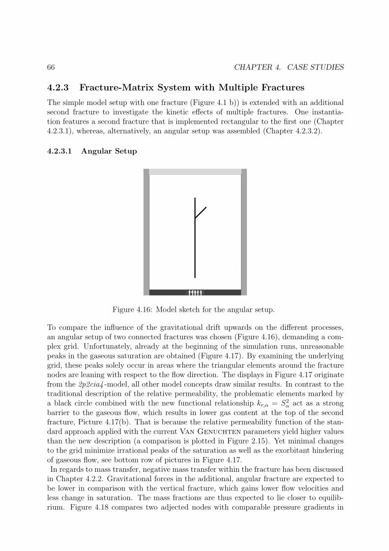
66 CHAPTER 4. CASE STUDIES
4.2.3 Fracture-Matrix System with Multiple Fractures
The simple model setup with one fracture (Figure 4.1 b)) is extended with an additionalsecond fracture to investigate the kinetic effects of multiple fractures. One instantia-tion features a second fracture that is implemented rectangular to the first one (Chapter4.2.3.1), whereas, alternatively, an angular setup was assembled (Chapter 4.2.3.2).
4.2.3.1 Angular Setup
Figure 4.16: Model sketch for the angular setup.
To compare the influence of the gravitational drift upwards on the different processes,an angular setup of two connected fractures was chosen (Figure 4.16), demanding a com-plex grid. Unfortunately, already at the beginning of the simulation runs, unreasonablepeaks in the gaseous saturation are obtained (Figure 4.17). By examining the underlyinggrid, these peaks solely occur in areas where the triangular elements around the fracturenodes are leaning with respect to the flow direction. The displays in Figure 4.17 originatefrom the 2p2cia4 -model, all other model concepts draw similar results. In contrast to thetraditional description of the relative permeability, the problematic elements marked bya black circle combined with the new functional relationship kr,α = S2
α act as a strongbarrier to the gaseous flow, which results in lower gas content at the top of the secondfracture, Picture 4.17(b). That is because the relative permeability function of the stan-dard approach applied with the current Van Genuchten parameters yield higher valuesthan the new description (a comparison is plotted in Figure 2.15). Yet minimal changesto the grid minimize irrational peaks of the saturation as well as the exorbitant hinderingof gaseous flow, see bottom row of pictures in Figure 4.17.In regards to mass transfer, negative mass transfer within the fracture has been discussed
in Chapter 4.2.2. Gravitational forces in the additional, angular fracture are expected tobe lower in comparison with the vertical fracture, which gains lower flow velocities andless change in saturation. The mass fractions are thus expected to lie closer to equilib-rium. Figure 4.18 compares two adjected nodes with comparable pressure gradients in

4.2. VERIFICATION STUDY FOR THE CONCEPTUAL MODELS 67
(a) Traditional relative perme-ability, unfortunate grid.
(b) kr,α = S2
α, unfortunate grid. (c) Applied grid, enlarged.
(d) Traditional relative perme-ability, better grid.
(e) kr,α = S2
α, better grid. (f) Improved grid, enlarged.
Figure 4.17: Dependancy on the applied grid, after 6 seconds.
both parts of the fracture system. Unfortunately, the distance from equilibrium is thatsmall that it can only be visualized by the whole mass transfer term IA
w of Equation (3.29).Still, non-equilibrium mass transfer is detected to be higher in the vertical fracture thanin the angular one, confirming a dependence on process velocity, or on driving forces foradvective flow, respectively. Note that the process of mass transfer is subject to the grid,so a comparison of both fracture parts strongly depends on the chosen nodes.Simulations were carried out until 150 seconds, the final distribution of the gaseous phase
is shown in Figure 4.19. Compared to the the angular fracture, gravitational forces pulla higher gas volume into the vertical part. However, the 2p2cia5 -model directs slightlymore gas into the angular fracture in comparison with the other drainage-bound models.

68 CHAPTER 4. CASE STUDIES
Figure 4.18: Mass transfer of air over the timespan of simulation for adjected nodes inthe vertical (dotted) and angular (solid) fracture.
(a) 2p2c, identical with 2p2cia4 - saturation Sn. (b) 2p2cia5 - saturation Sn.
Figure 4.19: Final state of the simulation runs which includes a second fracture.

4.2. VERIFICATION STUDY FOR THE CONCEPTUAL MODELS 69
4.2.3.2 Perpendicular Setup
Although the model setup is axially symmetrical, the grid generator is not forced tomesh symmetric, thus differences evolve between the left and the right half of the cappingfracture. However, symmetry demands that the underlying physical processes are identical
(a) Model sketch for the perpendicularsetup.
(b) Differences in element configuration betweenboth vertical branches.
for both branches, so any encountered deviation is of pure numerical origin. Whilstdifferences are observable for the propagation of the gaseous phase, they are present in allmodels. The right part of Figure 4.20 shows linear plots between the two arrows markedon the left picture, at a simulation time of 50 seconds. The upper subfigure comparesthe real mass fraction (solid) with the equilibrium mass fraction (dotted) of the 2p2cia5 -model, compared with the saturation of gas on the right axis. The lower subfigure presentsthe primary drainage-bound capillary pressure that is gained by the 2p2c-model (dashed)and the resolved capillary pressure of the unbound 2p2cia5 -model (solid). Compared tothe fluctuations of saturation, and thus also capillary pressure, the processes includedin the new interfacial-area based models (non-equilibrium mass transfer as well a betterdetermination of capillary pressure) do not enforce larger nonconformity. Nor do they, inregards to meshing, reduce numerical stability.

70 CHAPTER 4. CASE STUDIES
Figure 4.20: Deviances of XAw and pc gained by the 2p2cia5 -model (black, solid) with XA
w,s
(dotted) and the drainage-bound pc (dashed), in comparison with the saturation (grey).
Chapter 5
Final Remarks
5.1 Summary and Conclusion
An alternative to the standard approach to model multiphase multicomponent transporthas been presented which is able to eliminate the hysteretic behaviour of macroscale cap-illary pressure, and which is not bound on local thermodynamic equilibrium. The newapproach was implemented in the modeling framework DuMux, and several case scenarioswere assembled.Additionally, the distinct properties of fractures and their interconnection with the hostmatrix were regarded. Measurements determining upscaled effective parameters as wellas interfacial area which are gained through the work of Nuske (2009) have been imple-mented and proved to produce meaningful results on the larger scale. Numerical stabilitywas challenging with regards to the distinct differences between the fracture and thematrix, yet reasonable attempts improving mesh quality significantly enhanced the per-formance. While the new approach demands longer simulation time compared to thetraditional approach, numerical convergence was gained in equal measure. It is expectedthat further work, an implementation of an interface condition, for example, will furtherimprove performance and stability, and remaining numerical restrictions will dissolute.The new concept was verified for the test case of an infiltration of a gaseous phase intoa saturated, homogeneous domain. An application of conforming concepts for the rela-tive permeability function gained comparable results with regards to the gas distribution.Even when infiltrating into a fractured domain, no significant changes in phase distribu-tion between the different model concepts are observable. However, both additional effectsof the new approach, namely mass transfer due to non-equilibrium and process-dependingcapillary pressure, have been obtained. On the one hand, the new approach exhibits statesof non-equilibrium within the fracture due to high process velocities. The states are closerto a state of equilibrium if the flow regime is subject to smaller driving forces. However,the defining parameters (here especially the diffusion length) have to be further examinedto improve a correct estimation of the magnitude of such non-equilibrium processes. Onthe other hand, a determination of capillary pressure that is neither bound on drainage,nor on imbibition cycles, was successfully included in the numerical framework. A depen-dence besides the saturation on imbibition or drainage processes and process history isonce again monitored within the fracture.
71

72 CHAPTER 5. FINAL REMARKS
5.2 Outlook
To gain better insights into kinetic interphase mass transfer, the experimental knowledgeof the underlying processes has to be extended. Parameters which are necessary on themacroscale, such as the interface permeability Kwn, the production or destruction rateof interfacial area Ewn, or the diffusion length for microscale mass transfer d, have to befurther examined on the porescale to revoke current assumptions. If satisfactory infor-mation with regards to these underlying processes are gained through experiments, thephysically-based models can be verified and adjusted to match the experimental results.Future research has to be done to identify areas with significant local mass transfer ac-cording to process characteristics, possibly with a concept of dimensionless numbers (i.e.Damkohler number). A further interesting task would be to examine an example thatis capillary dominant with extensive drainage and imbibition cycles, where a physicallycorrect determination of capillary pressure is extremely important (for example the de-termination of recharge through the unsaturated zone for agricultural needs).A desirable employment to environmental applications of interest, such as CO2 injectioncomprising high flow velocities near the injection wells, requires improvements of the nu-merical framework. Multi-scale and multi-physics techniques save computing time anddata demand, thus reduce the compareatively larger simulation time of the new approach.Plus, the additional effective parameters have only to be collected in subdomains whereeffects of non-equilibrium are expected. Since even large systems in the range of kilome-ters call for a local determination of fine-scale mass transfer, refinement techniques arenecessary.Furthermore, the set of governing equations has to be extended for non-isothermal pro-cesses with energy balances. It is expected that mass transfer through non-equilibrium issignificant for non-isothermal applications such as thermally-enhanced soil remediation.As already mentioned, with regards to fracture-matrix systems, an interface condition isto be implemented. This will not only improve system stability and validity, but can fur-ther be extended to broaden the range of application to coupling procedures of differentflow regimes, i.e. flow through porous media coupled with free-flow. Then, even biologicapplications such as the transfer of therapeutic agents into and from the interstitium canbe examined.

Appendix A
Heterogeneous Setup with oneFracture
This section presents aditional visualizations of the test case of one single fracture, whichdo not have to be adressed in detail in the recent chapters.
73

74 APPENDIX A. HETEROGENEOUS SETUP WITH ONE FRACTURE
(a) 2p2c, identical with 2p2cia4 - saturation Sn. (b) 2p2cia5 - saturation Sn.
(c) 2p2cia5 - Equilibrium mass fraction of air
XAw,s.
(d) 2p2cia5 - Real mass fraction of air XAw .
Figure A.1: Final state of the simultation runs with one single fracture.
Bibliography
Atkins, P. W. and De Paula, J. (2006). Atkins’ Physical chemistry, volume 8. ed. OxfordUniversity Press.
Avraam, D. G. and Payatakes, A. C. (1995). Generalized relative permeability coeffi-cients during steady-state two-phase flow in porous media, correlation with the flowmechanisms. Transport in Porous Media, 20(1):135–168.
Bear, J. (1972). Dynamics of Fluids in Porous Media. Elsevier, New York.
Brooks, A. and Corey, A. (1964). Hydraulic Properties of Porous Media. In Hydrol. Pap.
Fort Collins, Colorado State University.
Class, H. (2001). Theorie und numerische Modellierung nichtisothermer Mehrphasen-
prozesse in NAPL–kontaminierten porosen Medien. PhD thesis, Mitteilungsheft 105,Institut fur Wasserbau, Universitat Stuttgart.
Coborny, O., Vomvoris, S., and Lanyon, G. W. (1994). Flow characterisation in crystallinerocks from combined continuum and stochastic fracture-flow models. In Dracos, T. andStauffer, F., editors, Transport and Reactive Processes in Aquifers, pages 311–316.
Cussler, E. L. (1997). Diffusion : mass transfer in fluid systems. Cambridge UniversityPress, 2nd ed. edition.
Dietrich, P., Helmig, R., Sauter, M., Holzl, H., Kongeter, J., and Teutsch, G. (2005). Flow
and Transport in Fractured Porous Media. Springer Verlag.
Flemisch, B., Fritz, J., Helmig, R., Niessner, J., and Wohlmuth, B. (2007). Dumux:a multi-scale multi-physics toolbox for flow and transport processes in porous media.ECCOMAS Thematic Conference on Multi-scale Computational Methods for Solids and
Fluids, page 8287.
Hassaini, M. Y., van Leer, B., and Rosendale, J. V. (1997). Upwind and high resolution
schemes. Springer.
Hassanizadeh, S. M. and Gray, W. G. (1980). General conservation equations for multi-phase systems: 3. constitutive theory for porous media ow. Advances in Water Re-
sources.
75

76 BIBLIOGRAPHY
Hassanizadeh, S. M. and Gray, W. G. (1990). Mechanics and thermodynamics of multi-phase flow in porous media including interphase boundaries. Adv. Water Resour., 13,
169-186.
Hassanizadeh, S. M. and Gray, W. G. (1993). Toward an improved description of thephysics of two-phase flow. Advances in Water Resources.
Helmig, R. (1997). Multiphase Flow and Transport Processes in the Subsurface. SpringerVerlag.
Helmig, R. and Huber, R. (1998). Comparison of galerkin-type discretization techniquesfor two-phase flow in heterogeneous porous media. Advances in Water Resources,21(8):697 – 711.
Jakobs, H. (2004). Simulation nicht-isothermer Gas-Wasser-Prozesse in komplexen Kluft-
Matrix-Systemen. PhD thesis, Institut fur Wasserbau, Universitat Stuttgart.
Joekar-Niasar, V., Hassanizadeh, S. M., and Leijnse, A. (2007). Insights into therelation-ships among capillary pressure, saturation, interfacial area and relative permeabilityusing pore-network modeling. Transport in Porous Media.
Johnson, L. H. (2002). Project Opalinus Clay: Safety report : Demonstration of disposal
feasibility for spent fuel, vitrified high-level waste and long-lived intermediate-level waste.NAGRA, Nationale Genossenschaft fr die Lagerung Radioaktiver Abflle.
Johnson, L. H., Marshall, P., Zuidema, P., and Gribi, P. (2004). Effects of post disposal
gas generation in a repository for spent fuel, high level waste and long lived intermediate
level waste sited in opalinus clay. NAGRA, Nationale Genossenschaft fr die LagerungRadioaktiver Abfalle.
Long, J., Aydin, A., Brown, S., Einstein, H., Hestir, K., Hsieh, P., Myer, L., Nolte, K.,Norton, D., Olsson, O., Paillet, F., Smith, J., and Thomson, L., editors (1996). Rock
Fractures and Fluid Flow: Contemporary Understanding and Applications. CommitteeOn Fracture Characterization And Fluid Flow, National Academies Press.
Millington, R. and Quirk, J. (1961). Permeability of porous solids. Trans. Faraday Soc.,57:1200–1207.
Niessner, J. and Hassanizadeh, S. (2008a). A model for two-phase flow in porous mediaincluding fluid-fluid interfacial area. Water Resour. Res., 44.
Niessner, J. and Hassanizadeh, S. (2008b). Modeling kinetic interphase mass transferfor two-phase flow in porous media including fluid-fluid interfacial area. submittet to:
Transport in Porous Media.
Niessner, J. and Hassanizadeh, S. (2009). Multiphase Flow Research, chapter Two-PhaseFlow and Transport in Porous Media Including Fluid-Fluid Interfacial Area. NovaScience Publishers.

BIBLIOGRAPHY 77
Nuske, K. P. (2009). Determination of interfacial area - capillary pressure - saturationrelationships for a single fracture. Master’s thesis, Universitat Stuttgart.
Rompp, H., Falbe, J., and Amelingmeier, E. (1999). Rompp - Lexikon Chemie. ThiemeVerlag, Stuttgart.
Sheta, H. (1999). Simulation von Mehrphasenvorgangen in porosen Medien unter Ein-
beziehung von Hysterese–Effekten. PhD thesis, Mitteilungsheft 100, Institut fur Wasser-bau, Universitat Stuttgart.
Silberhorn-Hemminger, A. (2002). Modellierung von Kluftaquifersystemen: Geostatistis-
che Analyse und deterministisch-stochastische Kluftgenerierung. PhD thesis, Institutfur Wasserbau, Universitat Stuttgart.
Smart, N. (2008). The effect of radiation on the anaerobic corrosion of steel. Journal of
Nuclear Materials, 379.
Somasundaram, T., Lynden-Bell, R. M., and Patterson, C. H. (1999). The passage ofgases through the liquid water/vapour interface: a simulation study. PCCP - Phys.
Chem. Chem. Phys, 1:143–148.
Van Genuchten, M. (1980). A closed-form equation for predicting the hydraulic conduc-tivity of unsaturated soils. Soil Sci. Soc. Am. J., 44:892–898.
Wolff, M. (2008). Comparison of mathematical and numerical models for twophase flowin porous media. Master’s thesis, Institut fur Wasserbau, Universitat Stuttgart.
Yang, C., Samper, J., Molinero, J., and Bonilla, M. (2007). Modelling geochemical andmicrobial consumption of dissolved oxygen after backfilling a high level radiactive wasterepository. Journal of Contaminant Hydrology, 93:130 – 148.

78 BIBLIOGRAPHY