Two Distinct Modes of Tropical Indian Ocean Precipitation

Two Distinct Modes of Tropical Indian Ocean Precipitation in Boreal Winterand Their Impacts on Equatorial Western Pacific*

BO WU AND TIANJUN ZHOU

LASG, Institute of Atmospheric Physics, Chinese Academy of Sciences, Beijing, China

TIM LI

IPRC, and Department of Meteorology, University of Hawaii at Manoa, Honolulu, Hawaii

(Manuscript received 30 January 2011, in final form 18 August 2011)

ABSTRACT

The observational analysis reveals two distinct precipitation modes, the zonal dipole (DP) mode and the

monopole (MP) mode, in the tropical Indian Ocean (TIO) during the El Nino mature winter, even though sea

surface temperature anomalies (SSTAs) have a similar basinwide warming pattern [referred to as the Indian

Ocean basin mode (IOBM)]. The formation of the two precipitation modes depends on the distinct evolutions

of the SSTA in the tropical Pacific and Indian Ocean. Both of the precipitation modes are preceded by an

Indian Ocean dipole (IOD). The IOD associated with the DP mode developed in late summer and was

triggered by Pacific El Nino through a ‘‘Sumatra–Philippine pattern.’’ The IOD associated with the MP mode

developed in early summer when the Pacific SSTAs were still normal. The different IOD onset time leads to

salient differences in subsequent evolution including the transfer of a dipole SST pattern to a basinwide

pattern. As a result, in the boreal winter, the zonal SSTA gradient associated with the DP mode is much

stronger than that associated with the MP mode. The strong SSTA zonal gradient associated with the DP

mode drives an anomalous Walker circulation in the TIO, while the nearly uniform warm SSTA associated

with the MP mode forces a basin-scale upward motion. The two modes have opposite impacts on the zonal

wind over the equatorial western Pacific, with anomalous westerly (easterly) occurring during the DP (MP)

mode, and thus they may have distinct impacts on El Nino evolution.

1. Introduction

During ENSO mature winter, the sea surface temper-

ature anomalies (SSTAs) in the tropical Indian Ocean

(TIO) evolve to a basin-scale uniform mode, referred to

as Indian Ocean basin mode (IOBM) (Klein et al. 1999;

Huang and Kinter 2002; Krishnamurthy and Kirtman

2003). The IOBM is generally seen as a response to

ENSO remote forcing (Klein et al. 1999; Venzke et al.

2000; Alexander et al. 2002; Lau and Nath 2003). The

warm SSTA in the equatorial central-eastern Pacific

stimulate an anomalous Walker circulation whose de-

scending branch would suppress the convection over the

eastern TIO and thus influence the atmospheric circula-

tion over the TIO. The suppressed convection would in-

crease the downward shortwave radiative flux, and the

low-level wind anomalies would decrease the upward

latent heat flux (Klein et al. 1999). Meanwhile, the anti-

cyclonic wind stress anomalies would excite oceanic

Rossby waves (Huang and Kinter 2002; Yu et al. 2005).

When the Rossby waves propagate westward to the

southwestern TIO, where the climatological thermocline

is shallow, it would warm the SSTA there (Xie et al. 2002;

Baquero-Bernal and Latif 2005). Therefore, both surface

thermal forcing and oceanic subsurface dynamics con-

tribute to the formation of the IOBM (Hong et al. 2010).

In addition, the variation of the oceanic mixed layer depth

plays a role in the TIO warming (Lau and Nath 2003).

The Indian Ocean dipole mode (IOD), which usually

develops in boreal summer and reaches a peak phase in

boreal fall (Saji et al. 1999; Webster et al. 1999), is

* School of Ocean and Earth Science and Technology Contri-

bution Number 8523 and the International Pacific Research Center

Contribution Number 831.

Corresponding author address: B. Wu, LASG, Institute of At-

mospheric Physics, Chinese Academy of Sciences, Beijing 100029,

China.

E-mail: [email protected]

1 FEBRUARY 2012 W U E T A L . 921

DOI: 10.1175/JCLI-D-11-00065.1

� 2012 American Meteorological Society

another air–sea coupled mode that may influence the

occurrence of the IOBM (Li et al. 2003; Hong et al.

2010). During summer and fall, the IOD, especially its

eastern pole, develops and maintains through a positive

‘‘wind–evaporation–SST’’ feedback— the cold SSTAs

suppress local convection and thus stimulate an anoma-

lous anticyclone over the southern TIO; in turn, the

southeasterly anomalies to the northeastern flank of

the anticyclone, which is in the same direction with the

background mean wind, further cool the SSTA by en-

hancing local evaporation, coastal upwelling and mixing

(Li et al. 2002, 2003; Shinoda et al. 2004). The operation

of the positive feedback relies on the maintenance of

the mean southeasterly wind. However, with the onset

of the Asian winter monsoon, the mean northwesterly

gradually replaces the southeasterly and controls the

coast of Sumatra. The change in the mean wind causes

the positive feedback transfer to a negative feedback that

damps the cold SSTA quickly (Li et al. 2003; Tokinaga

and Tanimoto 2004).

On the other hand, during boreal summer and fall, the

easterly anomalies over the equatorial Indian Ocean,

excited by the negative heating over the southeastern

TIO would stimulate oceanic downwelling Rossby waves

propagating westward (Yu et al. 2005). The Rossby waves

reflect to equatorial downwelling Kelvin waves in the

western boundary (Yuan and Liu 2009). After the Kelvin

waves reach the eastern TIO, it would help the negative

SSTA to damp and transfer to the positive SSTA (Li et al.

2003; Yuan and Liu 2009). The studies above suggested

that the evolution from IOD to IOBM is attributed to

the combined effects of the local negative feedback and

the oceanic wave dynamics.

As a dominant mode in the TIO, the IOBM may exert

a great impact on the variability in the tropical Pacific.

During El Nino decaying summer, with the decay of warm

SSTA in the central-eastern Pacific, the IOBM plays an

important role in the maintenance of the western North

Pacific (WNP) anomalous anticyclone (WNPAC) (Yang

et al. 2007; Li et al. 2008; Xie et al. 2009; Wu et al. 2009a,

2010; Huang et al. 2010), and thus has a strong impact on

the East Asian summer monsoon.

However, whether the IOBM has a great effect on the

tropical Pacific during El Nino mature winter is still a

controversial issue because of the presence of strong

El Nino remote forcing. Using a linearized model forced

by a basin-wide warm SSTA pattern, Watanabe and Jin

(2002) showed that the IOBM may induce an anomalous

anticyclone in the WNP through induced basin-wide

convection anomaly over the TIO. A similar experiment

but with a different model was done by Annamalai et al.

(2005a), who emphasized the role of SSTA over the

southwestern TIO. The easterly wind stress anomalies

to the southern flank of the anomalous anticyclone in-

duced by the IOBM may stimulate oceanic upwelling

Kelvin waves and favor a fast termination of the El Nino

(Weisberg and Wang 1997a,b; Kim and Lau 2001; Lau

and Wu 2001; Kug and Kang 2006). In contrast, Wu et al.

(2009a) noted, based on observational data analyses, that

during El Nino mature winter, the convection over the

eastern TIO is suppressed by the descending branch of

the El Nino–induced anomalous Walker circulation. As

a result, the warm SSTA in the eastern TIO is a passive

response to El Nino remote forcing. On the other hand,

warm SSTA in the western TIO plays an active role in

forcing anomalous ascending motion. As a consequence

of the dipole precipitation anomaly pattern in the TIO,

a westerly wind anomaly rather than an eastern anomaly

should appear over the equatorial western Pacific.

A related question is whether or not the TIO vari-

ability can significantly contribute to the ENSO evolu-

tion. The clarification of the question may advance our

understanding of the interactive nature of the TIO and

tropical Pacific. As shown in section 3, the TIO has two

distinct modes of precipitation anomalies in boreal win-

ter. Though both the modes are associated with basin-

wide warming patterns, they have opposite impacts on

the zonal wind over the tropical western Pacific. In this

study we will analyze the two anomalous precipitation

modes, especially their formation mechanisms. We will

also explore their teleconnection patterns with the trop-

ical Pacific variability.

The rest of the paper is organized as follow. Datasets,

analysis methods, and model are described in section 2.

In section 3, we obtain two dominant modes of the TIO

precipitation during boreal winter through an EOF anal-

ysis. The differences in the precipitation, atmospheric

circulation, and SST anomalies between the two dom-

inant modes are investigated. In section 4, we present

possible mechanisms responsible for the formation of

the two distinct modes. The different impacts of the two

TIO precipitation modes on the atmospheric circulation

over the tropical western Pacific are investigated in sec-

tion 5. Section 6 summarizes the major findings.

2. Datasets, methods, and model

a. Datasets

The datasets used in the present study consist of 1)

precipitation data from the Global Precipitation Cli-

matology Project (GPCP) (Adler et al. 2003); 2)

SST data from the Met Office (UKMO) Hadley

Center’s sea ice and SST dataset (HadISST) (Rayner

et al. 2003); 3) atmospheric circulation and surface

heat flux from the National Centers for Environment

Prediction (NCEP)–Department of Energy Atmospheric

922 J O U R N A L O F C L I M A T E VOLUME 25

Model Intercomparison Project II reanalysis (NCEP2)

(Kanamitsu et al. 2002); 4) ocean temperature and cir-

culation from the NCEP Global Ocean Data Assimi-

lation System (GODAS), which is forced by the

momentum flux, heat flux, and freshwater flux from the

NCEP2 (Behringer and Xue 2004). All the datasets

cover the period of 1979–2008, except for the GODAS

data, which are available over the period of 1980–2008.

In addition, the following datasets are used for the

comparison with the above datasets: 1) National Oceanic

and Atmospheric Administration (NOAA) interpolated

outgoing longwave radiation (OLR) (Liebmann and

Smith 1996); 2) the Climate Prediction Center (CPC)

Merged Analysis of Precipitation (CMAP) data (Xie

and Arkin 1997); 3) the surface heat flux in the reanalysis

data from the Japanese long-term reanalysis cooperative

research project (JRA-25) carried out by the Japan Me-

teorological Agency and the Central Research Institute

of Electric Power Industry (Onogi et al. 2007); 4) ocean

temperature and current derived from the Simple Ocean

Data Assimilation (SODA) (Carton et al. 2000); and

5) the National Centers for Environmental Prediction–

National Center for Atmospheric Research (NCEP–

NCAR) reanalysis data (Kalnay et al. 1996).

Following previous studies, IOD and Nino-3.4 indexes

are used to depict the IOD and ENSO. The IOD index

is defined as the difference of the area-averaged SSTA

between western (108S–108N, 508–708E) and eastern

TIO (108S–08, 908–1108E) in fall [September–November

(SON)], and the Nino-3.4 index is defined as the area-

averaged SSTA in the equatorial central-eastern Pacific

(58S–58N, 1708–1208W) in winter [December–February

(DJF)].

b. Methods

Because anomalous precipitation and associated dia-

batic heating, rather than the SSTA, have direct impacts

on the atmospheric circulation, we first analyze the two

dominant EOF modes of the DJF mean precipitation

anomalies over the TIO (158S–158N, 408–1108E). Cor-

responding atmospheric and oceanic anomalies are then

obtained through regressions against the time series of

normalized principle components (PCs). It is worth men-

tioning that the two distinct dominant patterns cannot be

derived from the DJF SSTA field in the TIO.

The robustness of the EOF results is carefully exam-

ined. First, we test the credibility of the precipitation data

by applying the same EOF analysis to the OLR data or

CMAP precipitation data. The obtained EOF spatial

patterns are generally similar to that derived from the

GPCP data, indicating that the results are not sensitive to

the data used. Second, we apply EOF analysis to 500-hPa

omega data for the period of 1950–2009 (NCEP–NCAR

reanalysis data). The obtained EOF spatial pattern is also

analogous to that derived from the GPCP data, suggest-

ing that the results are also insensitive to the analysis pe-

riod. Third, we test the credibility of the EOF analysis

method by comparing with a composite analysis. The years,

during which the normalized PC values are greater than 1.0

or less than 21.0 standard deviations, are selected to make

the composite analysis. The spatial pattern derived from the

composite is generally consistent with that derived from the

EOF analysis, indicating that the two dominant modes are

realistic. Because our focus is on the interannual variability,

variances longer than 8 years are filtered out through

a Lanczos filter prior to the analysis (Duchon 1979).

c. Model

In the study, a dry version of the Princeton AGCM

(Held and Suarez 1994) is used to assess the atmospheric

responses to specific heating over the TIO. Following

previous studies (Ting and Yu 1998; Jiang and Li 2005;

Li 2006), the model is linearized by specified realistic 3D

winter-mean (December–February) wind and temper-

ature fields. Based on the linearization, we can test the

model response to specific anomalous heating under the

realistic basic mean state. The model use a sigma vertical

coordinate with 5 evenly spaced levels from the top of

the atmosphere (s 5 0) to the surface (s 5 1). It has

a horizontal resolution of T42, equivalent to 2.88 3 2.88.

A more detailed description of the model can be found

in Jiang and Li (2005).

The model was used to study the low-level anomalous

anticyclone over the northeastern Indian Ocean during

El Nino developing summer (Wang et al. 2003) and the

reinitiation of the boreal summer intraseasonal oscilla-

tion over the TIO (Jiang and Li 2005).

3. Two dominant winter precipitation patterns andassociated large-scale circulations

The EOF analysis is applied to the DJF precipitation

anomaly field. The Rule N test based on the Monte Carlo

experiments is used to select the meaningful EOF mode

(Preisendorfer 1988; Li et al. 2000). The first three modes

pass the 5% significance level. The first and second modes

account for 25.2% and 14.4% of total variances, respec-

tively. According to the North role (North et al. 1982), the

two modes are well distinguished from each other and

from other modes.

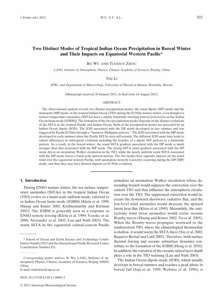
The spatial patterns of the first two leading modes are

shown in Figs. 1a,b. The TIO precipitation anomalies in

the EOF1 exhibit a dipole pattern, with a negative center

in the southeastern TIO and a positive center in the

western TIO. In contrast, the TIO precipitation anomalies

in the EOF2 generally exhibit a monopole pattern.


According to their distinct spatial patterns, the EOF1

and EOF2 are referred to as the dipole precipitation

(DP) mode and the monopole precipitation (MP) mode,

respectively.

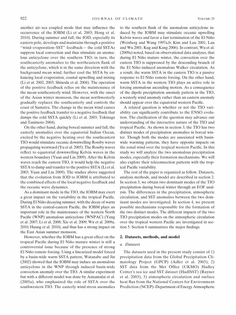
The time series of principal components (PCs) of the

two modes are shown in Fig. 1e. The power spectrum

densities and red noises of the PCs are shown in Fig. 2.

The PC1 has a major spectral peak in 2–3 yr and a sec-

ondary peak in 4–5 yr, while the PC2 has a major spectral

peak in 5 yr and a secondary peak in 2–3 yr.

Though the precipitation anomalies in the TIO are

distinct, both the modes correspond to a similar basin-

wide warming in the TIO at a first glance (Figs. 1c,d).

However, in fact, the spatial structures of the IOBM in

the two modes also have differences. For the MP mode,

the warm SSTA in the TIO is quite uniform, while the

SSTA associated with the DP mode shows a strong zonal

gradient, with the warm SSTA in the western TIO being

much stronger than that in the eastern TIO.

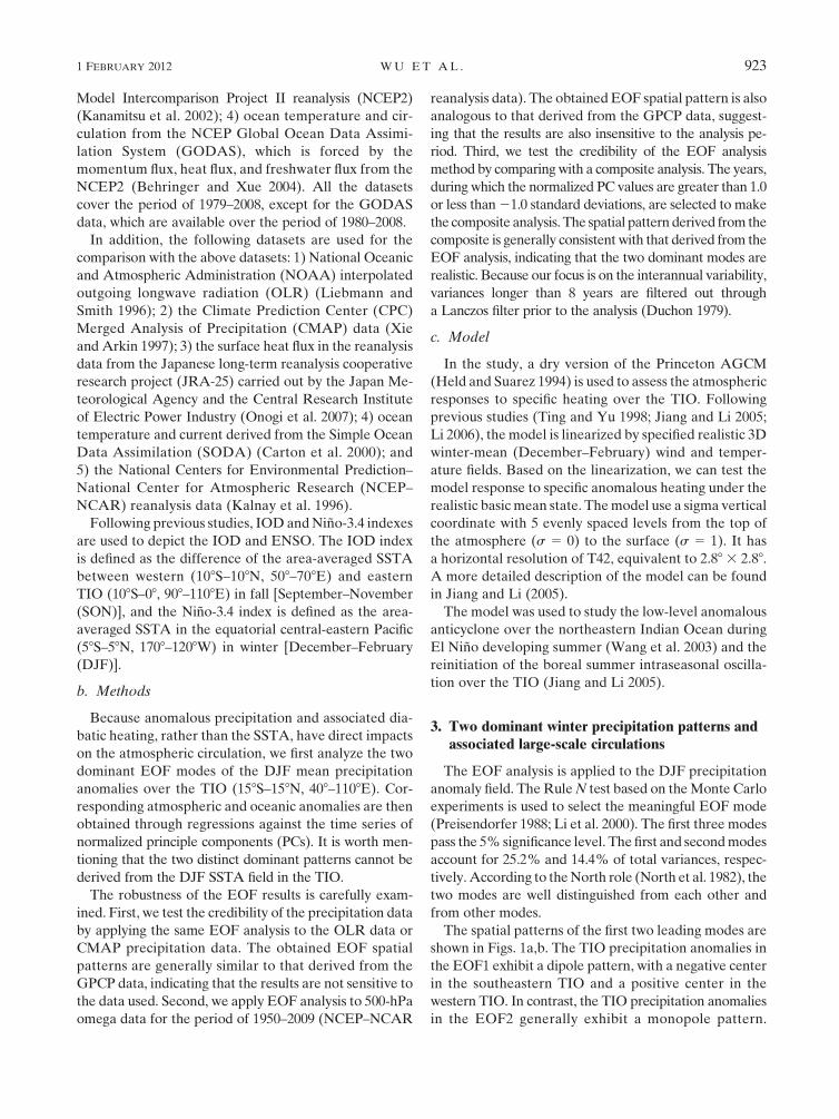
The different SSTA patterns correspond to different

zonal atmospheric circulation anomalies. Figure 3 shows

200-hPa velocity potential. For the DP mode, a diver-

gence over the tropical central-eastern Pacific connects

a divergence to its west, whose center is located over the

eastern TIO, Maritime Continent and tropical western

Pacific (Fig. 3a). Almost the entire TIO is covered by the

convergence, except for the far western TIO, indicating

that the vertical motion over the TIO is suppressed by

the descending branch of the anomalous Walker circu-

lation excited by the anomalous ascent motion over

the equatorial central-eastern Pacific (Chou 2004; Ham

et al. 2007; Wu et al. 2009a). For the MP mode, a well-

organized zonal tripole structure is seen over the tropi-

cal Pacific and TIO (Fig. 3b). Two divergences over the

TIO and central-eastern Pacific grip a convergence over

the tropical western Pacific and Maritime Continent.

The divergence over the TIO is stronger and more sig-

nificant than that over the central Pacific, implying that

FIG. 1. (a) The DJF-mean precipitation anomalies (GPCP; units: mm day21) and the cor-

responding 925-hPa wind anomalies (NCEP2; units: m s21) regressed onto the principal

component of the first EOF mode (DP mode). (b) As in (a), but for the second EOF mode (MP

mode). (c),(d) As in (a),(b), but for the SSTA (HadISST; units: K). (e) Normalized principal

components of the first and second EOF modes.


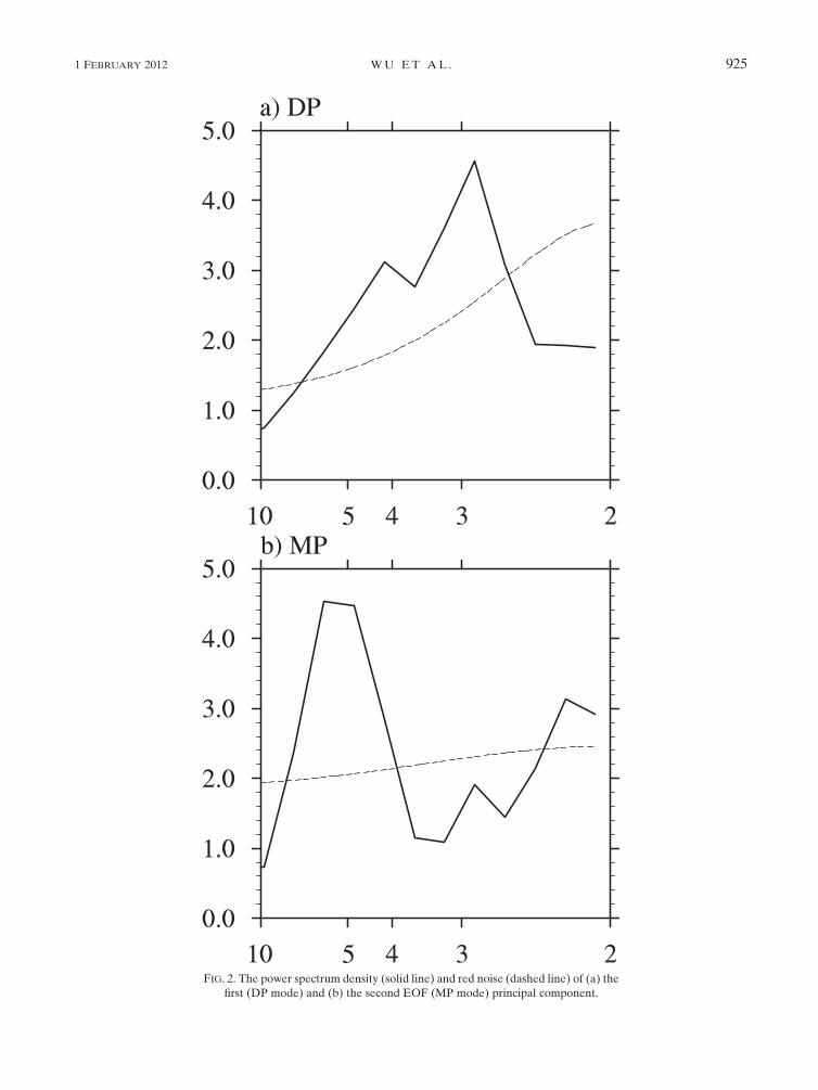
FIG. 2. The power spectrum density (solid line) and red noise (dashed line) of (a) the

first (DP mode) and (b) the second EOF (MP mode) principal component.


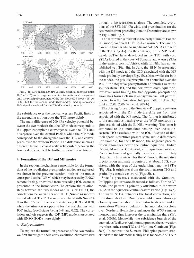
the subsidence over the tropical western Pacific links to

the ascending motion over the TIO more tightly.

The main difference of 200-hPa velocity potential be-

tween the two modes is that the DP mode corresponds to

the upper-tropospheric convergence over the TIO and

divergence over the central Pacific, while the MP mode

corresponds to the divergence over the TIO and conver-

gence over the western Pacific. The difference implies a

different Indian Ocean–Pacific relationship between the

two modes, which will be further explored in section 5.

4. Formation of the DP and MP modes

In the section, mechanisms responsible for the forma-

tions of the two distinct precipitation modes are explored.

As shown in the previous section, both of the modes

correspond to the IOBM, which may be caused by ENSO

remote forcing, or evolved from preceding IOD event as

presented in the introduction. To explore the relation-

ships between the two modes and IOD or ENSO, the

correlations between PCs and IOD (Nino-3.4) indexes

are calculated. The PC1 is more correlated with Nino-3.4

than the PC2, with the coefficients being 0.59 and 0.38,

while the situation is opposite for the correlations with

IOD index (coefficients being 0.44 and 0.62). The corre-

lation analysis suggests that DP (MP) mode is associated

with ENSO (IOD) more tightly.

a. Early evolution

To explore the formation processes of the two modes,

we first investigate their early evolution characteristics

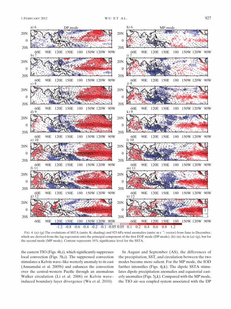
through a lag-regression analysis. The complete evolu-

tions of the SST, 925-hPa wind, and precipitations for the

two modes from preceding June to December are shown

in Fig. 4 and Fig. 5.

The difference is evident in the early summer. For the

DP mode, canonical El Nino–like warm SSTAs are ap-

parent in June, while no significant cold SSTAs are seen

in the TIO (Fig. 4a). On the contrary, for the MP mode,

dipole SSTAs have developed in the TIO, with cold

SSTAs located in the coast of Sumatra and warm SSTAs

in the eastern coast of Africa, while El Nino has not es-

tablished yet (Fig. 4h). In July, the El Nino associated

with the DP mode and the IOD associated with the MP

mode gradually develop (Figs. 4b,i). Meanwhile, for both

the modes, the positive precipitation anomalies over the

WNP, the negative precipitation anomalies over the

southeastern TIO, and the northward cross-equatorial

low-level wind linking the two opposite precipitation

anomalies form a classical antisymmetric Gill pattern,

referred to as the ‘‘Sumatra–Philippine pattern’’ (Figs. 5b,i,

Li et al. 2002, 2006; Wu et al. 2009b).

The driving forces to the Sumatra–Philippine patterns

associated with the DP mode are different from that

associated with the MP mode. The former is attributed

to the anomalous heating over the WNP monsoon re-

gion associated with the El Nino warming. The latter is

attributed to the anomalous heating over the south-

eastern TIO associated with the IOD. Because of that,

their spatial structures present some subtle differences.

For example, for the DP mode, the negative precipi-

tation anomalies cover the entire equatorial Indian

Ocean, Maritime Continent, and equatorial western

Pacific in June and gradually move southward in July

(Figs. 5a,b). In contrast, for the MP mode, the negative

precipitation anomaly is centered at about 108S, con-

sistent with the area of the underlying negative SSTA

(Fig. 5h). It originates from the southeastern TIO and

gradually extends eastward (Figs. 5h,i).

Specific processes associated with the Sumatra–

Philippine patterns are discussed as follows. For the DP

mode, the pattern is primarily attributed to the warm

SSTA in the equatorial central-eastern Pacific (Figs. 4a,b).

The warm SSTA enhances the local convection, and

thus stimulates twin Rossby wave–like anomalous cy-

clones symmetric about the equator to its west and an

anomalous Walker circulation. The anomalous cyclone

over Northern Hemisphere enhances the WNP summer

monsoon and thus increases the precipitation there (Wu

et al. 2009b). Meanwhile, the subsidence branch of the

anomalous Walker circulation suppressed the convection

over the southeastern TIO and Maritime Continent (Figs.

5a,b). In contrast, the Sumatra–Philippine pattern asso-

ciated with the MP mode mainly links to the cold SSTA in

FIG. 3. (a) DJF-mean 200-hPa velocity potential (contour units:

1026 m2 s21) and divergence wind (vector units: m s21) regressed

onto the principal component of the first mode (DP mode). (b) As

in (a), but for the second mode (MP mode). Shading represents

10% significance level for the 200-hPa velocity potential.


the eastern TIO (Figs. 4h,i), which significantly suppresses

local convection (Figs. 5h,i). The suppressed convection

stimulates a Kelvin wave–like westerly anomaly to its east

(Annamalai et al. 2005b) and enhances the convection

over the central-western Pacific through an anomalous

Walker circulation (Li et al. 2006) or Kelvin wave–

induced boundary layer divergence (Wu et al. 2010).

In August and September (AS), the differences of

the precipitation, SST, and circulation between the two

modes become more salient. For the MP mode, the IOD

further intensifies (Figs. 4j,k). The dipole SSTA stimu-

lates dipole precipitation anomalies and equatorial east-

erly anomalies (Figs. 5j,k). Compared with the MP mode,

the TIO air–sea coupled system associated with the DP

FIG. 4. (a)–(g) The evolutions of SSTA (units: K; shading) and 925-hPa wind anomalies (units: m s21; vector) from June to December,

which are derived from the lag regression onto the principal component of the first EOF mode (DP mode). (h)–(n) As in (a)–(g), but for

the second mode (MP mode). Contour represents 10% significance level for the SSTA.


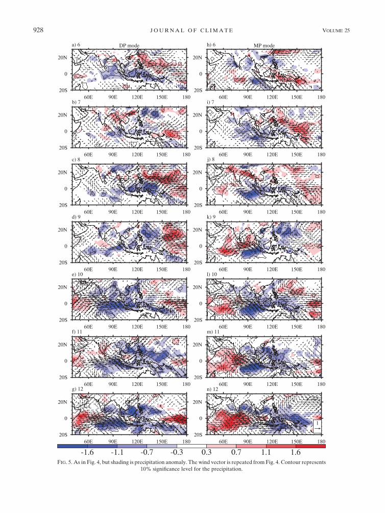
FIG. 5. As in Fig. 4, but shading is precipitation anomaly. The wind vector is repeated from Fig. 4. Contour represents

10% significance level for the precipitation.


mode develops much slower. The cold SSTA in the

southeastern TIO just slightly strengthens and SSTA is

hardly seen in the western TIO (Figs. 4c,d). Though the

negative precipitation anomalies in the eastern equatorial

Indian Ocean extend westward with the enhancement of

the El Nino remote forcing, the low-level wind anomalies

over the TIO are still scattered (Figs. 5c,d).

In October, the IOD associated with the MP mode

reaches peak phase, especially the warm SSTA of the

western pole being much stronger than the preceding

AS (Fig. 4l). The warm SSTA center is located in the

southwestern TIO, where the climatological thermocline

is shallow at the time. The SSTA results from the com-

bined effects of the oceanic Rossby wave (Xie et al. 2002;

Du et al. 2009) and surface latent heat flux (Wu and Yeh

2010). Correspondingly, the anomalous precipitation,

equatorial easterly, and southern TIO anomalous an-

ticyclone (SIOAC) are much stronger than that seen in

the AS (Fig. 5l). For the DP mode, with the warm SSTA

developing in the far western TIO, an IOD-like SSTA

pattern establishes (Fig. 4e). Correspondingly, the dipole

precipitation pattern, equatorial easterly anomalies and

SIOAC also form (Fig. 5e). However, it is worth noting

that the spatial structure of the IOD associated with the

DP mode is different from that associated with the MP

mode. For the DP mode, the warm SSTA of the western

pole is mainly located in the far northwestern TIO and

the coast of Africa, so that the zonal distance between the

two poles of the IOD is much larger than that associated

with the MP mode. Correspondingly, the positive pre-

cipitation anomalies in the western TIO are shifted

westward, and the negative precipitation anomalies in

the eastern TIO extend westward. The equatorial east-

erly anomalies extend westward 208 farther than that

associated with the MP mode, and the SIOAC is also

shifted westward.

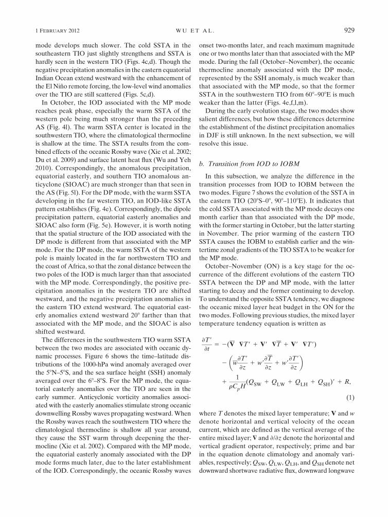
The differences in the southwestern TIO warm SSTA

between the two modes are associated with oceanic dy-

namic processes. Figure 6 shows the time–latitude dis-

tributions of the 1000-hPa wind anomaly averaged over

the 58N–58S, and the sea surface height (SSH) anomaly

averaged over the 68–88S. For the MP mode, the equa-

torial easterly anomalies over the TIO are seen in the

early summer. Anticyclonic vorticity anomalies associ-

ated with the easterly anomalies stimulate strong oceanic

downwelling Rossby waves propagating westward. When

the Rossby waves reach the southwestern TIO where the

climatological thermocline is shallow all year around,

they cause the SST warm through deepening the ther-

mocline (Xie et al. 2002). Compared with the MP mode,

the equatorial easterly anomaly associated with the DP

mode forms much later, due to the later establishment

of the IOD. Correspondingly, the oceanic Rossby waves

onset two-months later, and reach maximum magnitude

one or two months later than that associated with the MP

mode. During the fall (October–November), the oceanic

thermocline anomaly associated with the DP mode,

represented by the SSH anomaly, is much weaker than

that associated with the MP mode, so that the former

SSTA in the southwestern TIO from 608–908E is much

weaker than the latter (Figs. 4e,f,l,m).

During the early evolution stage, the two modes show

salient differences, but how these differences determine

the establishment of the distinct precipitation anomalies

in DJF is still unknown. In the next subsection, we will

resolve this issue.

b. Transition from IOD to IOBM

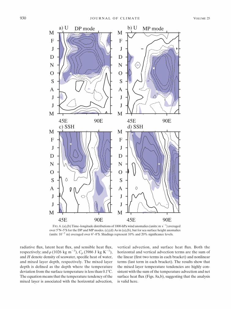
In this subsection, we analyze the difference in the

transition processes from IOD to IOBM between the

two modes. Figure 7 shows the evolution of the SSTA in

the eastern TIO (208S–08, 908–1108E). It indicates that

the cold SSTA associated with the MP mode decays one

month earlier than that associated with the DP mode,

with the former starting in October, but the latter starting

in November. The prior warming of the eastern TIO

SSTA causes the IOBM to establish earlier and the win-

tertime zonal gradients of the TIO SSTA to be weaker for

the MP mode.

October–November (ON) is a key stage for the oc-

currence of the different evolutions of the eastern TIO

SSTA between the DP and MP mode, with the latter

starting to decay and the former continuing to develop.

To understand the opposite SSTA tendency, we diagnose

the oceanic mixed layer heat budget in the ON for the

two modes. Following previous studies, the mixed layer

temperature tendency equation is written as

›T9

›t5 2(V � $T9 1 V9 � $T 1 V9 � $T9)

2 w›T9

›z1 w9

›T

›z1 w9

›T9

›z

� �

11

rCpH(QSW 1 QLW 1 QLH 1 QSH)9 1 R,

(1)

where T denotes the mixed layer temperature; V and w

denote horizontal and vertical velocity of the ocean

current, which are defined as the vertical average of the

entire mixed layer; $ and ›/›z denote the horizontal and

vertical gradient operator, respectively; prime and bar

in the equation denote climatology and anomaly vari-

ables, respectively; QSW, QLW, QLH, and QSH denote net

downward shortwave radiative flux, downward longwave


radiative flux, latent heat flux, and sensible heat flux,

respectively; and r (1026 kg m23), Cp (3986 J kg K21),

and H denote density of seawater, specific heat of water,

and mixed layer depth, respectively. The mixed layer

depth is defined as the depth where the temperature

deviation from the surface temperature is less than 0.18C.

The equation means that the temperature tendency of the

mixed layer is associated with the horizontal advection,

vertical advection, and surface heat flux. Both the

horizontal and vertical advection terms are the sum of

the linear (first two terms in each bracket) and nonlinear

terms (last term in each bracket). The results show that

the mixed layer temperature tendencies are highly con-

sistent with the sum of the temperature advection and net

surface heat flux (Figs. 8a,b), suggesting that the analysis

is valid here.

FIG. 6. (a),(b) Time–longitude distributions of 1000-hPa wind anomalies (units: m s21) averaged

over 58N–58S for the DP and MP modes. (c),(d) As in (a),(b), but for sea surface height anomalies

(units: 1022 m) averaged over 68–88S. Shadings represent 10% and 20% significance levels.


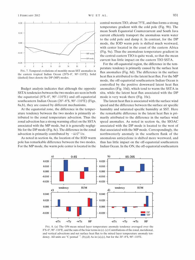
Budget analysis indicates that although the opposite

SSTA tendencies between the two modes are seen in both

the equatorial (88S–08, 908–1108E) and off-equatorial

southeastern Indian Ocean (208–88S, 908–1108E) (Figs.

8a,b), they are caused by different mechanisms.

At the equatorial zone, the difference in the temper-

ature tendency between the two modes is primarily at-

tributed to the zonal temperature advection. Thus the

zonal advection has a strong warming effect on the SSTA

associated with the MP mode, but it is generally negligi-

ble for the DP mode (Fig. 8c). The difference in the zonal

advection is primarily contributed by 2u›T9/›x.

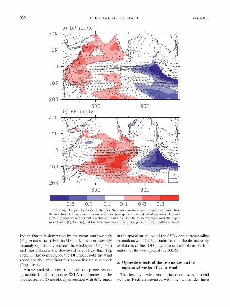
As noted in section 4a, the location of the IOD warm

pole has remarkable difference between the two modes.

For the MP mode, the warm pole center is located in the

central-western TIO, about 758E, and thus forms a strong

temperature gradient with the cold pole (Fig. 9b). The

mean South Equatorial Countercurrent and South Java

current efficiently transport the anomalous warm water

to the cold pole and damp it. In contrast, for the DP

mode, the IOD warm pole is shifted much westward,

with center located in the coast of the eastern Africa

(Fig. 9a). Thus the anomalous temperature gradient in

the central-eastern TIO is quite weak, so that the mean

current has little impact on the eastern TIO SSTA.

For the off-equatorial region, the difference in the tem-

perature tendency is primarily caused by the surface heat

flux anomalies (Fig. 8d). The difference in the surface

heat flux is attributed to the latent heat flux. For the MP

mode, the off-equatorial southeastern Indian Ocean is

controlled by the positive downward latent heat flux

anomalies (Fig. 10d), which tend to warm the SSTA in

situ, while the latent heat flux associated with the DP

mode is very weak there (Fig. 10c).

The latent heat flux is associated with the surface wind

speed and the difference between the surface air specific

humidity and saturated specific humidity at SST. Here

the remarkable difference in the latent heat flux is pri-

marily attributed to the difference in the surface wind

speed anomalies. As noted in section 4a, the SIOAC

associated with the DP mode is located to the west of

that associated with the MP mode. Correspondingly, the

northwesterly anomaly in the southern flank of the

anomalous anticyclone is shifted more westward, and

thus has little impact on the off-equatorial southeastern

Indian Ocean. In the ON, the off-equatorial southeastern

FIG. 7. Temporal evolutions of monthly mean SST anomalies in

the eastern tropical Indian Ocean (208S–08, 908–1108E). Solid

(dashed) lines denote the DP (MP) modes.

FIG. 8. (a) The ON-mean mixed layer temperature anomaly tendency averaged over the

88S–08, 908–1108E, and the sum of the four terms in (c). (c) Contributions of the zonal, meridional,

and vertical advections and net surface heat flux to the mixed layer temperature anomaly ten-

dency. All units are 8C pentad21. (b),(d) As in (a),(c), but for the 208–88S, 908–1108E.


Indian Ocean is dominated by the mean southwesterly

(Figure not shown). For the MP mode, the northwesterly

anomaly significantly reduces the wind speed (Fig. 10b)

and thus enhances the downward latent heat flux (Fig.

10d). On the contrary, for the DP mode, both the wind

speed and the latent heat flux anomalies are very week

(Figs. 10a,c).

Above analysis shows that both the processes re-

sponsible for the opposite SSTA tendencies in the

southeastern TIO are closely associated with differences

in the spatial structures of the SSTA and corresponding

anomalous wind fields. It indicates that the distinct early

evolutions of the IOD play an essential role in the for-

mation of the two types of the IOBM.

5. Opposite effects of the two modes on theequatorial western Pacific wind

The low-level wind anomalies over the equatorial

western Pacific associated with the two modes have

FIG. 9. (a) The spatial patterns of October–November mean oceanic temperature anomalies,

derived from the lag regression onto the first principal component (shading, units: 8C), and

climatological oceanic currents (vector, units: m s21). Both fields are averaged over the upper

mixed layer. (b) As in (a), but for the second mode. Contour represents 10% significance level.


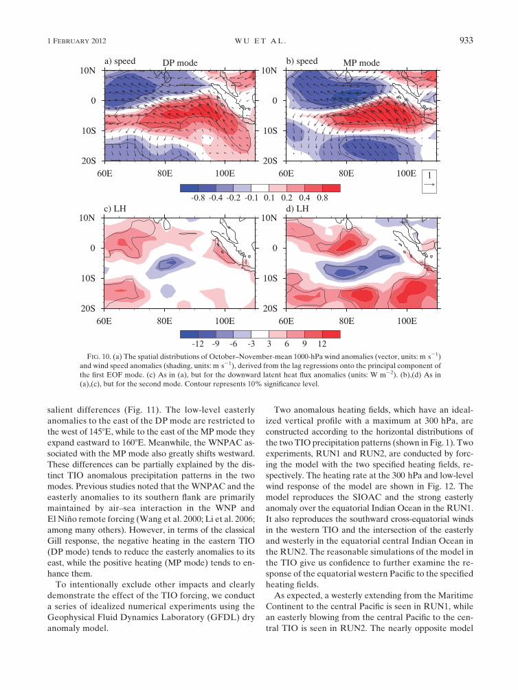
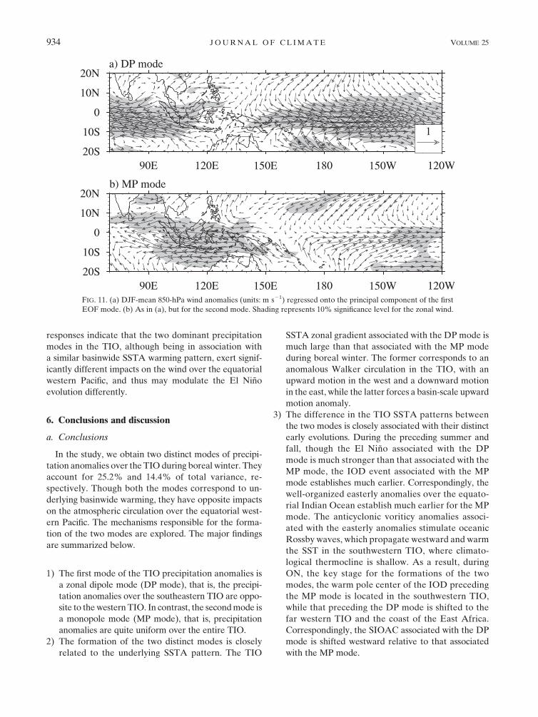
salient differences (Fig. 11). The low-level easterly

anomalies to the east of the DP mode are restricted to

the west of 1458E, while to the east of the MP mode they

expand eastward to 1608E. Meanwhile, the WNPAC as-

sociated with the MP mode also greatly shifts westward.

These differences can be partially explained by the dis-

tinct TIO anomalous precipitation patterns in the two

modes. Previous studies noted that the WNPAC and the

easterly anomalies to its southern flank are primarily

maintained by air–sea interaction in the WNP and

El Nino remote forcing (Wang et al. 2000; Li et al. 2006;

among many others). However, in terms of the classical

Gill response, the negative heating in the eastern TIO

(DP mode) tends to reduce the easterly anomalies to its

east, while the positive heating (MP mode) tends to en-

hance them.

To intentionally exclude other impacts and clearly

demonstrate the effect of the TIO forcing, we conduct

a series of idealized numerical experiments using the

Geophysical Fluid Dynamics Laboratory (GFDL) dry

anomaly model.

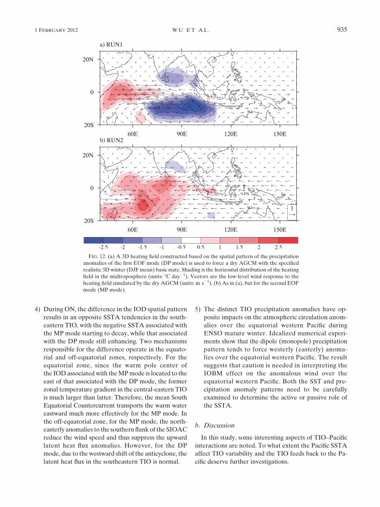
Two anomalous heating fields, which have an ideal-

ized vertical profile with a maximum at 300 hPa, are

constructed according to the horizontal distributions of

the two TIO precipitation patterns (shown in Fig. 1). Two

experiments, RUN1 and RUN2, are conducted by forc-

ing the model with the two specified heating fields, re-

spectively. The heating rate at the 300 hPa and low-level

wind response of the model are shown in Fig. 12. The

model reproduces the SIOAC and the strong easterly

anomaly over the equatorial Indian Ocean in the RUN1.

It also reproduces the southward cross-equatorial winds

in the western TIO and the intersection of the easterly

and westerly in the equatorial central Indian Ocean in

the RUN2. The reasonable simulations of the model in

the TIO give us confidence to further examine the re-

sponse of the equatorial western Pacific to the specified

heating fields.

As expected, a westerly extending from the Maritime

Continent to the central Pacific is seen in RUN1, while

an easterly blowing from the central Pacific to the cen-

tral TIO is seen in RUN2. The nearly opposite model

FIG. 10. (a) The spatial distributions of October–November-mean 1000-hPa wind anomalies (vector, units: m s21)

and wind speed anomalies (shading, units: m s21), derived from the lag regressions onto the principal component of

the first EOF mode. (c) As in (a), but for the downward latent heat flux anomalies (units: W m22). (b),(d) As in

(a),(c), but for the second mode. Contour represents 10% significance level.


responses indicate that the two dominant precipitation

modes in the TIO, although being in association with

a similar basinwide SSTA warming pattern, exert signif-

icantly different impacts on the wind over the equatorial

western Pacific, and thus may modulate the El Nino

evolution differently.

6. Conclusions and discussion

a. Conclusions

In the study, we obtain two distinct modes of precipi-

tation anomalies over the TIO during boreal winter. They

account for 25.2% and 14.4% of total variance, re-

spectively. Though both the modes correspond to un-

derlying basinwide warming, they have opposite impacts

on the atmospheric circulation over the equatorial west-

ern Pacific. The mechanisms responsible for the forma-

tion of the two modes are explored. The major findings

are summarized below.

1) The first mode of the TIO precipitation anomalies is

a zonal dipole mode (DP mode), that is, the precipi-

tation anomalies over the southeastern TIO are oppo-

site to the western TIO. In contrast, the second mode is

a monopole mode (MP mode), that is, precipitation

anomalies are quite uniform over the entire TIO.

2) The formation of the two distinct modes is closely

related to the underlying SSTA pattern. The TIO

SSTA zonal gradient associated with the DP mode is

much large than that associated with the MP mode

during boreal winter. The former corresponds to an

anomalous Walker circulation in the TIO, with an

upward motion in the west and a downward motion

in the east, while the latter forces a basin-scale upward

motion anomaly.

3) The difference in the TIO SSTA patterns between

the two modes is closely associated with their distinct

early evolutions. During the preceding summer and

fall, though the El Nino associated with the DP

mode is much stronger than that associated with the

MP mode, the IOD event associated with the MP

mode establishes much earlier. Correspondingly, the

well-organized easterly anomalies over the equato-

rial Indian Ocean establish much earlier for the MP

mode. The anticyclonic voriticy anomalies associ-

ated with the easterly anomalies stimulate oceanic

Rossby waves, which propagate westward and warm

the SST in the southwestern TIO, where climato-

logical thermocline is shallow. As a result, during

ON, the key stage for the formations of the two

modes, the warm pole center of the IOD preceding

the MP mode is located in the southwestern TIO,

while that preceding the DP mode is shifted to the

far western TIO and the coast of the East Africa.

Correspondingly, the SIOAC associated with the DP

mode is shifted westward relative to that associated

with the MP mode.

FIG. 11. (a) DJF-mean 850-hPa wind anomalies (units: m s21) regressed onto the principal component of the first

EOF mode. (b) As in (a), but for the second mode. Shading represents 10% significance level for the zonal wind.


4) During ON, the difference in the IOD spatial pattern

results in an opposite SSTA tendencies in the south-

eastern TIO, with the negative SSTA associated with

the MP mode starting to decay, while that associated

with the DP mode still enhancing. Two mechanisms

responsible for the difference operate in the equato-

rial and off-equatorial zones, respectively. For the

equatorial zone, since the warm pole center of

the IOD associated with the MP mode is located to the

east of that associated with the DP mode, the former

zonal temperature gradient in the central-eastern TIO

is much larger than latter. Therefore, the mean South

Equatorial Countercurrent transports the warm water

eastward much more effectively for the MP mode. In

the off-equatorial zone, for the MP mode, the north-

easterly anomalies to the southern flank of the SIOAC

reduce the wind speed and thus suppress the upward

latent heat flux anomalies. However, for the DP

mode, due to the westward shift of the anticyclone, the

latent heat flux in the southeastern TIO is normal.

5) The distinct TIO precipitation anomalies have op-

posite impacts on the atmospheric circulation anom-

alies over the equatorial western Pacific during

ENSO mature winter. Idealized numerical experi-

ments show that the dipole (monopole) precipitation

pattern tends to force westerly (easterly) anoma-

lies over the equatorial western Pacific. The result

suggests that caution is needed in interpreting the

IOBM effect on the anomalous wind over the

equatorial western Pacific. Both the SST and pre-

cipitation anomaly patterns need to be carefully

examined to determine the active or passive role of

the SSTA.

b. Discussion

In this study, some interesting aspects of TIO–Pacific

interactions are noted. To what extent the Pacific SSTA

affect TIO variability and the TIO feeds back to the Pa-

cific deserve further investigations.

FIG. 12. (a) A 3D heating field constructed based on the spatial pattern of the precipitation

anomalies of the first EOF mode (DP mode) is used to force a dry AGCM with the specified

realistic 3D winter (DJF mean) basic state. Shading is the horizontal distribution of the heating

field in the midtroposphere (units: 8C day21). Vectors are the low-level wind response to the

heating field simulated by the dry AGCM (units: m s21). (b) As in (a), but for the second EOF

mode (MP mode).


1) The differences in the surface wind over the equato-

rial western Pacific between the two modes may

further influence SSTA evolution in the equatorial

central-eastern Pacific. For the MP mode, the IOD-

related SSTA establishes prior to the SSTA in the

equatorial central-eastern Pacific (Figs. 4h,i). The

negative pole of the IOD suppresses local convection

and thus stimulates Kelvin wave–like westerly anom-

alies to its east, extending to the equatorial central

Pacific. The westerly anomalies would contribute to

the onset and development of ENSO, suggesting that

IOD may be one of triggering factors of ENSO, if it

established prior to ENSO (Saji and Yamagata 2003).

2) The DP and MP modes would have opposite contri-

butions to ENSO phase transition through the op-

posite impacts on the low-level wind anomalies over

the equatorial western Pacific during boreal winter.

In terms of a lag-regression analysis, the SSTA in the

equatorial central-eastern Pacific associated with the

MP mode tend to transform to an opposite phase

earlier than that associated with the DP mode (Figure

not shown). The stronger easterly wind anomalies

to the east of the MP mode may stimulate stronger

oceanic upwelling Kelvin waves, which propagate

eastward and accelerate El Nino decaying.

3) Though the EOF and lead–lag analyses indicate that

the TIO variability associated with the MP mode tends

to influence the low-level wind variability over the

tropical Pacific, caution is needed to interpret the

relationship between the MP mode and ENSO. In

addition to remote forcing from the Indian Ocean,

ENSO is primarily modulated by a variety of air–sea

interaction processes in the Pacific. For example,

three typical MP mode years, 1980, 1982, and 1994,

have different TIO–Pacific relationships. They all have

a strong IOD event, but only 1982 has a strong ENSO

event. 1980 is a normal year, while 1994 is a weak

El Nino year (Meyers et al. 2007). This is consistent

with the fact that the MP mode only has weak cor-

relation with Nino-3.4 index (section 4a).

We found that the MP modes are closely linked to the

preceding IOD. However, the initiation of the IOD is

still unknown. Our preliminary analysis indicates that

the IOD associated with the MP mode is trigged by a

shoaling of the thermocline in the eastern equatorial

Indian Ocean. In the preceding year of the IOD initia-

tion, Rossby waves in the southern off-equatorial Indian

Ocean propagate westward and reflect to Kelvin waves

in the East African coast, which propagate eastward and

shoal the thermocline in the eastern tropical Indian

Ocean (Rao et al. 2009). The mechanism responsible for

the IOD initiation deserves further studies.

Major conclusions from this study are obtained from

the observational analysis. They should be further tested

and explored by numerical experiments. We analyzed

twentieth-century experiments (20C3M) of the some

coupled general circulation models that participated in

phase 3 of the Coupled Model Intercomparison Project

(CMIP3). All runs are integrated from the 1850 to the

present. It is found that the UKMO Hadley Centre gen-

eral circulation model version 1 (UKMO-HADGEM1)

reproduces the DP and MP modes analogous to the

observation (figure not shown). Since the 150-yr model

output provides much larger sample sets, we plan to

analyze the long integration result to reveal statistically

significant features. We will also diagnose models that

failed to reproduce the two distinct precipitation modes.

In addition, idealized numerical experiments may be

conducted to investigate specific processes responsible

for the remote El Nino impact on the TIO and the

effect of the TIO SSTA on the Pacific SST and wind

evolution.

Acknowledgments. This work was supported by NSFC

Grant 41005040, National Program on Key Basic Re-

search Project (2010CB951904), and National High-

Tech Research and Development Plan of China

(2010AA012302). TL was supported by ONR Grants

N000140810256 and N000141010774 and by the Inter-

national Pacific Research Center that is sponsored by

the Japan Agency for Marine-Earth Science and Tech-

nology (JAMSTEC), NASA (NNX07AG53G), and

NOAA (NA17RJ1230).

REFERENCES

Adler, R. F., and Coauthors, 2003: The version-2 Global Pre-

cipitation Climatology Project (GPCP) monthly precipitation

analysis (1979–present). J. Hydrometeor., 4, 1147–1167.

Alexander, M. A., I. Blade, M. Newman, J. R. Lanzante, N.-C. Lau,

and J. D. Scott, 2002: The atmospheric bridge: The influence of

ENSO teleconnections on air–sea interaction over the global

oceans. J. Climate, 15, 2205–2231.

Annamalai, H., P. Liu, and S.-P. Xie, 2005a: Southwest Indian

Ocean SST variability: Its local effect and remote influence on

Asian monsoons. J. Climate, 18, 4150–4167.

——, S.-P. Xie, J. P. McCreay, and R. Murtgudde, 2005b: Impact of

Indian Ocean surface temperature on developing El Nino.

J. Climate, 18, 302–319.

Baquero-Bernal, A., and M. Latif, 2005: Wind-driven oceanic

Rossby waves in the tropical South Indian Ocean with and

without an active ENSO. J. Phys. Oceanogr., 35, 729–746.

Behringer, D. W., and Y. Xue, 2004: Evaluation of the global

ocean data assimilation system at NCEP: The Pacific Ocean.

Preprints, Eighth Symp. on Integrated Observing and Assimi-

lation Systems for Atmosphere, Oceans, and Land Surface,

Seattle, WA, Amer. Meteor. Soc., 2.3. [Available online at

http://ams.confex.com/ams/84Annual/techprogram/paper_

70720.htm.]


Carton, J. A., G. Chepurin, and X. H. Cao, 2000: A Simple Ocean

Data Assimilation analysis of the global upper ocean 1950–95.

Part II: Results. J. Phys. Oceanogr., 30, 311–326.

Chou, C., 2004: Establishment of the low-level wind anomalies over

the western North Pacific during ENSO development. J. Climate,

17, 2195–2212.

Du, Y., S.-P. Xie, G. Huang, and K. Hu, 2009: Role of air–sea in-

teraction in the long persistence of El Nino–induced North

Indian Ocean warming. J. Climate, 22, 2023–2038.

Duchon, C., 1979: Lanczos filtering in one and two dimensions.

J. Appl. Meteor., 18, 1016–1022.

Ham, Y.-G., J.-S. Kug, and I.-S. Kang, 2007: Role of moist energy

advection in formulating anomalous Walker circulation asso-

ciated with El Nino. J. Geophys. Res., 112, D24105, doi:10.1029/

2007JD008744.

Held, I. M., and M. J. Suarez, 1994: A proposal for the inter-

comparison of the dynamical cores of atmospheric general

circulation models. Bull. Amer. Meteor. Soc., 75, 1825–1830.

Hong, C.-C., T. Li, L. Ho, and Y.-C. Chen, 2010: Asymmetry of the

Indian Ocean basinwide SST anomalies: Roles of ENSO and

IOD. J. Climate, 23, 3563–3576.

Huang, B. H., and J. L. Kinter, 2002: Interannual variability in the

tropical Indian Ocean. J. Geophys. Res., 107, 3199, doi:10.1029/

2001JC001278.

Huang, G., K. Hu, and S.-P. Xie, 2010: Strengthening of tropical

Indian Ocean teleconnection to the Northwest Pacific since

the mid-1970s: An atmospheric GCM study. J. Climate, 23,

5294–5304.

Jiang, X. A., and T. Li, 2005: Reinitiation of the boreal summer

intraseasonal oscillation in the tropical Indian Ocean. J.

Climate, 18, 3777–3795.

Kalnay, E., and Coauthors, 1996: The NCEP/NCAR 40-Year Re-

analysis Project. Bull. Amer. Meteor. Soc., 77, 437–472.

Kanamitsu, M., W. Ebisuzaki, J. Woollen, S.-K. Yang, J. J. Hnilo,

M. Fiorino, and G. L. Potter, 2002: NCEP-DOE AMIP-II

Reanalysis (R-2). Bull. Amer. Meteor. Soc., 83, 1631–1643.

Kim, K. M., and K. M. Lau, 2001: Dynamics of monsoon-induced

biennial variability in ENSO. Geophys. Res. Lett., 28, 315–318.

Klein, S. A., B. J. Soden, and N. C. Lau, 1999: Remote sea surface

temperature variations during ENSO: Evidence for a tropical

atmospheric bridge. J. Climate, 12, 917–932.

Krishnamurthy, V., and B. P. Kirtman, 2003: Variability of the

Indian Ocean: Relation to monsoon and ENSO. Quart. J. Roy.

Meteor. Soc., 129, 1623–1646.

Kug, J. S., and I. S. Kang, 2006: Interactive feedback between

ENSO and the Indian Ocean. J. Climate, 19, 1784–1801.

Lau, K. M., and H. T. Wu, 2001: Principal modes of rainfall–SST

variability of the Asian summer monsoon: A reassessment of

monsoon–ENSO relationship. J. Climate, 14, 2880–2895.

Lau, N.-C., and M. J. Nath, 2003: Atmosphere–ocean variations in

the Indo-Pacific sector during ENSO episodes. J. Climate, 16,

3–20.

Li, S. L., J. Lu, G. Huang, and K. M. Hu, 2008: Tropical Indian

Ocean basin warming and East Asian summer monsoon: A

multiple AGCM study. J. Climate, 21, 6080–6088.

Li, T., 2006: Origin of the summertime synoptic-scale wave train in

the western North Pacific. J. Atmos. Sci., 63, 1093–1102.

——, Y. S. Zhang, E. Lu, and D. Wang, 2002: Relative role of

dynamic and thermodynamic processes in the development

of the Indian Ocean dipole. Geophys. Res. Lett., 29, 2110,

doi:10.1029/2002GL015789.

——, B. Wang, C. P. Chang, and Y. S. Zhang, 2003: A theory for the

Indian Ocean dipole-zonal mode. J. Atmos. Sci., 60, 2119–2135.

——, P. Liu, X. Fu, B. Wang, and G. A. Meehl, 2006: Spatiotem-

poral structures and mechanisms of the tropospheric biennial

oscillation in the Indo-Pacific warm ocean regions. J. Climate,

19, 3070–3087.

Li, X.-F., L. J. Pietrafesa, S.-F. Lan, and L.-A. Xie, 2000: Signifi-

cance test for empirical orthogonal function (EOF) analysis of

meteorological and oceanic data. Chin. J. Oceanology Lim-

nol., 18, 10–17.

Liebmann, B., and C. A. Smith, 1996: Description of a complete

(interpolated) outgoing longwave radiation dataset. Bull.

Amer. Meteor. Soc., 77, 1275–1277.

Meyers, G., P. McIntosh, L. Pigot, and M. Pook, 2007: The years of

El Nino, La Nina, and interactions with the tropical Indian

Ocean. J. Climate, 20, 2872–2880.

North, G. R., T. L. Bell, R. F. Cahalan, and F. J. Moeng, 1982:

Sampling errors in the estimation of empirical orthogonal

functions. Mon. Wea. Rev., 110, 699–706.

Onogi, K., and Coauthors, 2007: The JRA-25 Reanalysis. J. Meteor.

Soc. Japan, 85, 369–432.

Preisendorfer, R. W., 1988: Principal Component Analysis in Me-

teorology and Oceanography. Elsevier Science, 425 pp.

Rao, S. A., J.-J. Luo, S. K. Behera, and T. Yamagata, 2009: Gen-

eration and termination of Indian Ocean dipole events in 2003,

2006, and 2007. Climate Dyn., 33, 751–767.

Rayner, N. A., D. E. Parker, E. B. Horton, C. K. Folland, L. V.

Alexander, D. P. Rowell, E. C. Kent, and A. Kaplan, 2003:

Global analyses of sea surface temperature, sea ice, and night

marine air temperature since the late nineteenth century.

J. Geophys. Res., 108, 4407, doi:10.1029/2002JD002670.

Saji, N. H., and T. Yamagata, 2003: Structure of SST and surface

wind variability during Indian Ocean dipole mode events:

COADS observations. J. Climate, 16, 2735–2751.

——, B. N. Goswami, P. N. Vinayachandran, and T. Yamagata,

1999: A dipole mode in the tropical Indian Ocean. Nature, 401,

360–363.

Shinoda, T., M. A. Alexander, and H. H. Hendon, 2004: Remote

response of the Indian Ocean to interannual SST variations in

the tropical Pacific. J. Climate, 17, 362–372.

Ting, M. F., and L. H. Yu, 1998: Steady response to tropical heating

in wavy linear and nonlinear baroclinic models. J. Atmos. Sci.,

55, 3565–3582.

Tokinaga, H., and Y. Tanimoto, 2004: Seasonal transition of SST

anomalies in the tropical Indian ocean during El Nino and

Indian Ocean dipole years. J. Meteor. Soc. Japan, 82, 1007–

1018.

Venzke, S., M. Latif, and A. Villwock, 2000: The coupled GCM

ECHO-2. Part II: Indian Ocean response to ENSO. J. Climate,

13, 1371–1383.

Wang, B., R. G. Wu, and X. H. Fu, 2000: Pacific–East Asian tele-

connection: How does ENSO affect East Asian climate?

J. Climate, 13, 1517–1536.

——, ——, and T. Li, 2003: Atmosphere–warm ocean interaction

and its impacts on Asian–Australian monsoon variation.

J. Climate, 16, 1195–1211.

Watanabe, M., and F. F. Jin, 2002: Role of Indian ocean warming in

the development of Philippine Sea anticyclone during ENSO.

Geophys. Res. Lett., 29, 1478, doi:10.1029/2001GL014318.

Webster, P. J., A. M. Moore, J. P. Loschnigg, and R. R. Leben,

1999: Coupled ocean–temperature dynamics in the Indian

Ocean during 1997–98. Nature, 401, 356–360.

Weisberg, R. H., and C. Z. Wang, 1997a: A western Pacific oscil-

lator paradigm for the El Nino–Southern Oscillation. Geo-

phys. Res. Lett., 24, 779–782.


——, and ——, 1997b: Slow variability in the equatorial west-

central Pacific in relation to ENSO. J. Climate, 10, 1998–2017.

Wu, B., T. J. Zhou, and T. Li, 2009a: Seasonally evolving dominant

interannual variability modes of East Asian climate. J. Cli-

mate, 22, 2992–3005.

——, ——, and ——, 2009b: Contrast of rainfall–SST relationships

in the western North Pacific between the ENSO developing

and decaying summers. J. Climate, 16, 4398–4405.

——, T. Li, and T. J. Zhou, 2010: Relative role of Indian Ocean and

western North Pacific SST forcing in the East Asian summer

monsoon anomalies. J. Climate, 23, 2974–2986.

Wu, R., and S.-W. Yeh, 2010: A further study of the tropical Indian

Ocean asymmetric mode in boreal spring. J. Geophys. Res.,

115, D08101, doi:10.1029/2009JD012999.

Xie, P., and P. A. Arkin, 1997: Global precipitation: A 17-year

monthly analysis based on gauge observations, satellite

estimates, and numerical model outputs. Bull. Amer. Meteor.

Soc., 78, 2539–2558.

Xie, S.-P., H. Annamalai, F. A. Schott, and J. P. McCreary, 2002:

Structure and mechanisms of South Indian Ocean climate

variability. J. Climate, 15, 864–878.

——, K. Hu, J. Hafner, H. Tokinaga, Y. Du, G. Huang, and T. Sampe,

2009: Indian Ocean capacitor effect on Indo–western Pacific

climate during the summer following El Nino. J. Climate, 22,

730–747.

Yang, J. L., Q. Y. Liu, S.-P. Xie, Z. Y. Liu, and L. X. Wu, 2007:

Impact of the Indian Ocean SST basin mode on the Asian

summer monsoon. Geophys. Res. Lett., 34, L02708, doi:10.1029/

2006GL028571.

Yu, W. D., B. Q. Xiang, L. Liu, and N. Liu, 2005: Understanding

the origins of interannual thermocline variations in the tropi-

cal Indian Ocean. Geophys. Res. Lett., 32, L24706, doi:10.1029/

2005GL024327.

Yuan, D. L., and H. L. Liu, 2009: Long-wave dynamics of sea level

variations during Indian Ocean dipole events. J. Phys. Oce-

anogr., 39, 1115–1132.


Documents

Two Distinct Modes of Tropical Indian Ocean Precipitation