Two-Dimensional Vertical Reynolds-Averaged Navier-Stokes · PDF fileTwo-Dimensional Vertical Reynolds-Averaged Navier-Stokes Equations Versus One-Dimensional Saint-Venant Model for

Archives of Hydro-Engineering and Environmental MechanicsVol. 53 (2006), No. 4, pp. 295–309© IBW PAN, ISSN 1231–3726

Two-Dimensional Vertical Reynolds-Averaged Navier-StokesEquations Versus One-Dimensional Saint-Venant Model for

Rapidly Varied Open Channel Water Flow Modelling

Michał Szydłowski, Piotr Zima

Gdańsk University of Technology, Faculty for Civil and Environmental Engineering,ul. Narutowicza 11/12, 80-952 Gdańsk, Poland, e-mails: [email protected], [email protected]

(Received March 27, 2006; revised July 18, 2006)

AbstractThe paper concerns mathematical modelling of free surface open channel water flow. In orderto simulate the flow two models are used – two-dimensional vertical Reynolds-AveragedNavier-Stokes equations and one-dimensional Saint-Venant equations. The former is solvedwith SIPMLE algorithm of finite difference method using Marker and Cell technique to tracea free surface movement. The latter is solved using the finite volume method. The dam-break(water column collapse) problem on horizontal bottom is investigated as a test case. Thecalculated results are compared with each other. The numerical simulations are examinedagainst laboratory experiment presented by Koshizuka et al (1995). The possibility of usingthe described models to simulate rapidly varied flow is discussed.

Key words: mathematical modelling, Reynolds-Averaged Navier-Stokes equations, Saint-Venant equations, free surface flow, rapidly varied flow, dam-break problem

1. Introduction

During the last almost half century, a lot of work on mathematical modelling influid dynamics was carried out. The considerable progress in hardware and softwaredevelopment has made possible the use of mathematical models in engineering andindustry. The numerical solutions of equations describing hydrodynamics processesin open channels – being a part of computational fluid dynamics (CFD) – arealso intensively investigated. This development already started during the eighties(Abbott 1979, Cunge et al 1980, Granatowicz and Szymkiewicz 1989) and continues(Fletcher 1991, Anderson 1995, Szymkiewicz 2000).

The mathematical equations (representing fundamental laws of physics) that gov-ern the phenomenon of free surface water flow, the Navier-Stokes (NS) equations,are well known. However, their solution is practically impossible (despite currentcomputer powers) for the scale of any real case. Hence the simplified models areusually solved for numerical simulation of open channel flow. The most widely used

296 M. Szydłowski, P. Zima

models of one-dimensional flow are the Saint-Venant (SV) equations. They can bederived from NS equations using the spatial averaging procedure. In this paper wecompare numerical solutions for rapidly varied free surface flow in open channel,computed with two-dimensional vertical Reynolds-Averaged NS (RANS) equationsand one-dimensional SV model. The analysis will be useful to assess whether theSV equations constitute an adequate model of free surface water flow near somelocal effects (i.e. steep wave fronts, hydraulic jumps, etc.) or not and answer thequestion as to whether they can be used for simulation of typical water engineeringproblems.

2. Mathematical Models of Free Surface Water Flow

2.1. Navier-Stokes Equations

In general, the open channel water flow is a three dimensional time dependent,incompressible, fluid dynamics problem with a free surface. The well known NSequations (together with continuity equation) describe the dynamics of a portion ofany fluid (Sawicki 1998). However, the water flow in natural and artificial channelsand reservoirs is usually turbulent. In order to eliminate the problem of turbulencethe NS equations can be averaged in time to obtain RANS equations that describethe mean flow (Sawicki 1998). Then the effects of the turbulent fluctuations on themean flow can be imposed applying some turbulence models. The three dimensionalRANS model is often used in technical fluid mechanics, but is still too complex tobe applied to describe open channel flow for practical cases. Many numerical tech-niques for solving RANS equations have been successfully applied so far (Fletcher1991, Anderson 1995). They are usually based on the finite difference method(FDM), finite element method (FEM) or finite volume method (FVM). One of themost popular and often used technique is a SIMPLE scheme (Semi Implicit Methodfor Pressure Linked Equations) of FDM (Potter 1982). In this algorithm a divergenceof RANS equations is considered. It leads to the Poisson equation which describespressure field evolution (pressure-correction equation). In the study presented inthis paper the SIMPLE algorithm is used to solve two-dimensional vertical RANSequations on a rectangular, staggered grid.

If RANS model is used to describe the open channel flow the free surfacemovement problem must be solved. The free surface moves with the velocity ofthe fluid particles located at the boundary, and therefore its position must be foundduring computation. One of the techniques to solve this problem is the Markerand Cell (MAC) method (Welch et al 1966). The application of this method tosolve open channel flow is possible, but unique, due to huge computational powerneeded to simulate some real cases. Therefore, the solutions are often limited totwo dimensional (in the vertical plane) test cases (Maronnier et al 1999, Mohapatraet al 1999, Zima 2005, Zwart et al 1999).

Two-Dimensional Vertical Reynolds-Averaged Navier-Stokes Equations . . . 297

2.2. Saint-Venant Equations

Two-dimensional shallow water (SW) equations can be obtained from the RANSmodel using a depth averaging procedure (Szymkiewicz 2000). This process elimi-nates the free surface location problem from the solution. For the equations deriva-tion, it is assumed that the vertical component of velocity can be neglected, pressurefield is hydrostatic, bottom slope is small and bottom friction can be approximatedas for steady flow conditions. Therefore, SW equations are not a true mathematicalrepresentation of the free surface water flow, but they reduce one of the spatial di-mensions from the problem. Finally, two-dimensional SW equations can be reducedto the SV model considering only one-dimensional water flow in the channel. Ingeneral, Saint-Venant assumptions are not satisfied for rapidly varied flow in anopen channel and this model seems to be a poor representation of real phenomenaof the flow near local hydraulic effects. In this paper we present the comparisonbetween numerical solution to RANS and SV models for rapidly varied flow in anopen channel during the dam-break problem (collapse of water column) on a hori-zontal bottom. Unfortunately, the FDM and FEM numerical methods for SV modelsolution are often inefficient for modelling rapidly varied flow, when discontinuitieslike hydraulic jumps or steep fronts exist. In order to ensure the proper solution toSV equations the FVM is applied (Szydłowski 2004). The calculated results analysisillustrates the influence of RANS equations spatial averaging procedure leading tothe SV model on the quality of numerical simulation of rapidly varied free surfacewater flow.

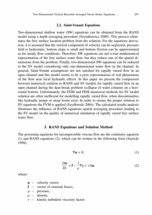
3. RANS Equations and Solution Method

The governing equations for incompressible viscous flow are the continuity equation(1) and RANS equations (2), which can be written in the following form (Sawicki1998):

∇u = 0, (1)

DuDt= f −

1ρ∇p + ν∆u, (2)

where:

u – velocity vector,f – vector of external forces,p – pressure,ρ – density,ν – kinetic turbulent viscosity factor.


If the divergence operator is applied, equation (2) can be rewritten as pressurecorrection equation (Potter 1982):

∆ p̄ = −∇ · (u · ∇u) , (3)

where p̄ denotes normalized pressure expressed as p̄ = p/ρ.In the vertical Cartesian plane x-y (neglecting one of the horizontal dimensions)

RANS equations are solved only for two velocity components (horizontal ux inx-direction and vertical uy in y-direction) and for the pressure p. The external bodyforces vector includes the acceleration due to gravity g with components ρg. Theequations (1, 2, 3) can be rewritten in differential form for both velocity componentsas follows:

∂ux

∂x+∂uy∂y= 0, (4)

∂ux

∂t+ ux∂ux

∂x+ uy∂ux

∂y= gx −

1ρ

∂p∂x+ ν

(∂2ux

∂x2 +∂2ux

∂y2

),

∂uy∂t+ ux∂uy∂x+ uy∂uy∂y= gy −

1ρ

∂p∂y+ ν

(∂2uy∂x2 +

∂2uy∂y2

),

(5)

∂2 p̄∂x2 +

∂2 p̄∂y2= −

(∂ux

∂x

)2

+ 2(∂ux

∂y

) (∂uy∂x

)+

(∂uy∂y

)2. (6)

Equations (5, 6) are solved using a SIMPLE algorithm of FDM. The mainidea of this method is applying the splitting technique to the solution. The firststep is a prediction of the velocity field integrating equations (5). The explicitscheme is used to obtain values of velocity components with values of pressurefrom previous time step. In the second step, the correction of pressure field iscomputed using equation (6). Then, it is used to correct the velocity field to satisfythe zero divergence condition (4).

In order to determine the free surface location the flow domain is defined usingthe MAC method (Welch et al 1966).

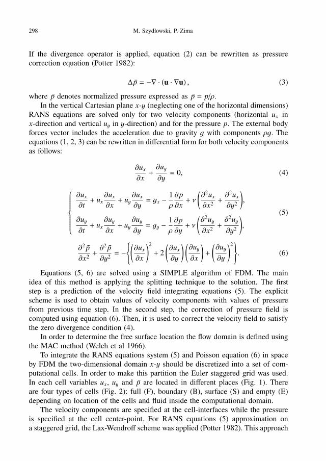
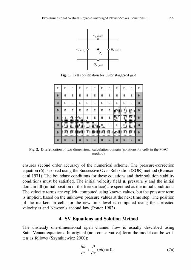
To integrate the RANS equations system (5) and Poisson equation (6) in spaceby FDM the two-dimensional domain x-y should be discretized into a set of com-putational cells. In order to make this partition the Euler staggered grid was used.In each cell variables ux, uy and p̄ are located in different places (Fig. 1). Thereare four types of cells (Fig. 2): full (F), boundary (B), surface (S) and empty (E)depending on location of the cells and fluid inside the computational domain.

The velocity components are specified at the cell-interfaces while the pressureis specified at the cell center-point. For RANS equations (5) approximation ona staggered grid, the Lax-Wendroff scheme was applied (Potter 1982). This approach


Fig. 1. Cell specification for Euler staggered grid

Fig. 2. Discretization of two-dimensional calculation domain (notations for cells in the MACmethod)

ensures second order accuracy of the numerical scheme. The pressure-correctionequation (6) is solved using the Successive Over-Relaxation (SOR) method (Remsonet al 1971). The boundary conditions for these equations and their solution stabilityconditions must be satisfied. The initial velocity field u, pressure p̄ and the initialdomain fill (initial position of the free surface) are specified as the initial conditions.The velocity terms are explicit, computed using known values, but the pressure termis implicit, based on the unknown pressure values at the next time step. The positionof the markers in cells for the new time level is computed using the correctedvelocity u and Newton’s second law (Potter 1982).

4. SV Equations and Solution Method

The unsteady one-dimensional open channel flow is usually described usingSaint-Venant equations. In original (non-conservative) form the model can be writ-ten as follows (Szymkiewicz 2000):

∂h∂t+∂

∂x(uh) = 0, (7a)


∂u∂t+ u∂u∂x+ g∂h∂x= g

(S0 − S f

), (7b)

where u is the flow mean velocity (depth averaged velocity component in x-direction– ux), h water depth, g acceleration due to gravity, x and t represent distance andtime and S0 and S f denote bed and friction slopes, respectively. The friction slopecan be defined by Manning’s formula, which for the rectangular channel of unitwidth has the form:

S f =n2u |u|h4/3 . (8)

The model (7a, b) describes gradually varied, one-dimensional free surface flow.Unfortunately, this non-conservative form of equations is inadequate when hydraulicjumps or steep water wave fronts can appear. It was proved (Abbott 1979) that thewater flow with discontinuities can be properly described using a conservative formof SV model only. This can be written in vector form as follows (Cunge et al 1980)

∂U∂ t+∂F∂ x+ S = 0, (9)

where:

U = h

uh

, F = uh

u2h + 0.5gh2

, S =

0

−gh(S0 − S f

) . (10a, b, c)

Equation (10) can be rewritten in equivalent form as

∂U∂ t+ div F + S = 0. (11)

In order to integrate the equations system (11) in space the FVM was cho-sen (LeVeque 2002). Applying this method one-dimensional domain x must bediscretized into the set of line segment cells (Fig. 3). Each cell is defined by itscentre-point and each flow parameter is averaged inside the cell.

∂Ui

∂ t∆xi +

(Fi+1/2 − Fi−1/2

)+

(Si+1/2 + Si−1/2

)∆xi = 0. (12)

In order to calculate the fluxes F at cell interfaces the Roe (1981) scheme isused. Detailed description of the method is available in the literature (Toro 1997,Szydłowski 2004, Zoppou and Roberts 2003) therefore it is omitted here. The sourceterms S are approximated using the method proposed by Bermudez and Vazquez


Fig. 3. Discretization of one-dimensional calculation domain

(1994). The numerical algorithm is completed with a two-step explicit scheme ofFDM for integration in time. This scheme is of second-order accuracy in time andits stability is restricted by Courant number (Potter 1982).

5. Numerical Calculations and Results Discussion

The mathematical models described in points 2 and 3 of this paper have beenused to simulate a CFD standard problem – dam-break flow test on the horizontalbottom. The problem is equivalent to the water column collapse effect. The flow ondry bottom downstream of the ‘dam’ was considered. Numerical results obtainedwith both models were compared. Moreover, the results of a laboratory experimentcarried out by Koshizuka et al (1995) were used to examine the calculations. It iswell known that the SV model is not a true mathematical representation of the freesurface water flow. However, shallow water models are commonly used for simulat-ing the dam-break flows, assuming that the vertical velocities and non-hydrostaticpressure distribution do not affect the long term results (Morris 2000, Szydłowski2003). In this analysis, we compare the numerical results for the free surface profilesand the front velocity obtained using SV and RANS models at the beginning of thewater flow process – immediately after water column collapse.

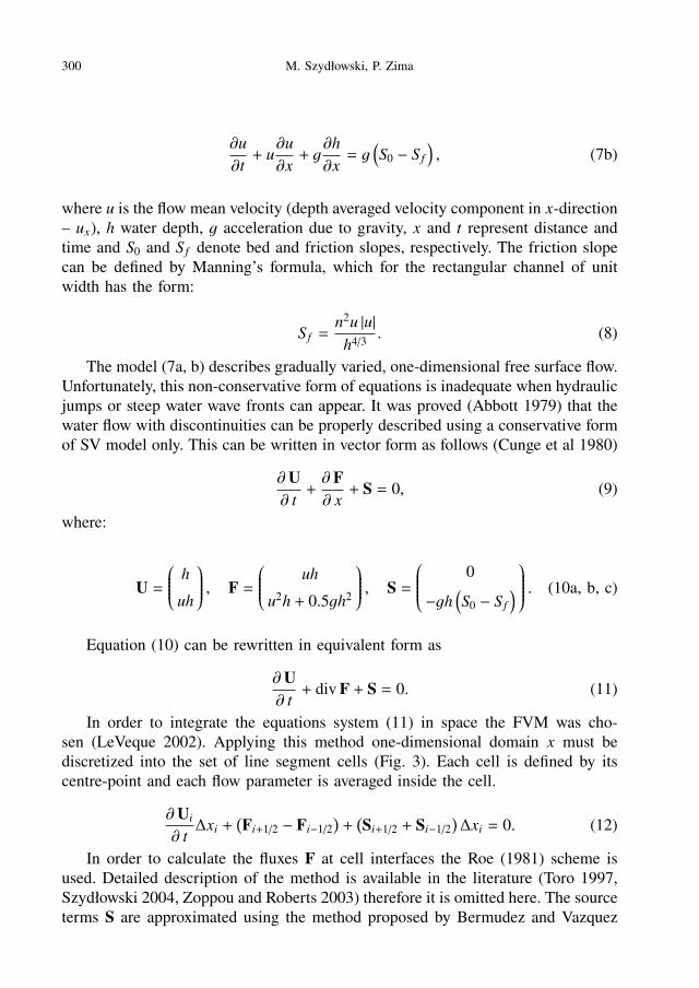
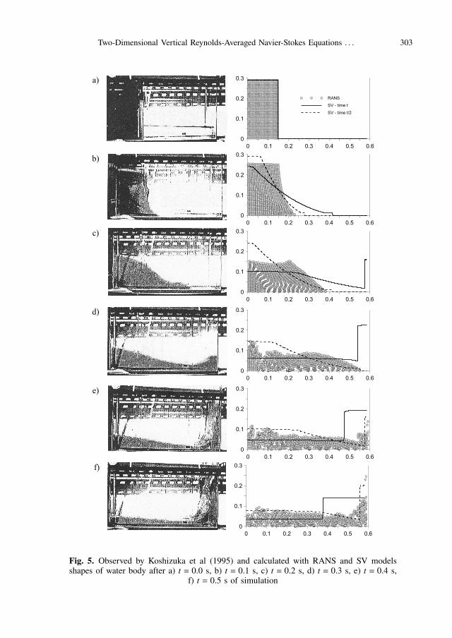
Geometry of domain and initial position of water column is presented in Fig-ure 4. In the laboratory experiment, a glass box with the scale L = 14.6 cm was used.The water column was supported by the vertical wall, which was drawn up rapidly(about 0.05 s) for the beginning of collapse. The experiment was recorded usinga video camera. Some pictures of water body during the experiment are presentedin Figure 5. Before the ‘dam-break’ the water body was at rest. After sudden waterrelease, two effects were observed – depression of water table travelling upstreamand steep water front going downstream of the initial water surface discontinuity.After reaching the box wall, the wave moving downstream reflects there, forminga sudden surface swelling going upstream. Moreover, a water splash effect can beobserved near the wall.

The numerical simulation with RANS model with the following parameterswas carried out: number of cells 1891 (∆x = ∆y = 0.973 cm), number of particlesn = 800. Gravitation unit gy = −9.806 ms−2 and turbulent kinetic viscosity factorν = 10−3 m2s−1 were imposed. However, viscous effect on the bottom and walls ofthe channel was neglected – the slip boundary condition was imposed there.


Fig. 4. Geometry of domain and initial shape of water column

Numerical simulation with SV model was carried out using a mesh composedof 1169 computational cells (∆x = 0.0005 m). Time integration was done usinga two-step explicit scheme with time step ∆t = 0.0001 s ensuring solution stability.In the first simulation a bottom friction was neglected. The slip boundary conditionon the channel bottom for RANS equations and Manning coefficient equal to zeroin SV model are equivalent to the frictionless open channel flow case. This as-sumption makes computed results possible to compare with others. Moreover, thissimplification is not far from the test case, where the flow over a glass surface ofsmall friction is considered.

The free surface profiles obtained using an SV model for different times isshown in Fig. 5 as solid lines. The results of computing with RANS model (particleslocations only) for the example calculation are presented in the same Figure as thecircle marks.

In order to analyse the wave front propagation problem the flow was considereduntil the front have touched the vertical box wall. The position of the water front isoverestimated by the SV model, as compared with the numerical solution to RANSequations. It was observed that the wave front approximated with SV model is abouttwo times faster than that computed with RANS model or an observed one. Thiseffect can also be seen watching the shapes of water table computed with SV modelfor times equal to half the simulation time (dotted line in Fig. 5). The water levelfor these moments fits the RANS computations and observations quite well.

The front location discrepancy is a result of difference of wave front propagationvelocity predicted using SV and RANS equations. The distance travelled by the frontas a function of time for numerical simulations and experiments is shown in Fig. 6.

The measurements and computed results in non-dimensional relation x/L areshown on the normalized time (tn = t

√2g/L) background. The slope of the curve

defines the velocity of the wave front. The significant disagreement between SV


Fig. 5. Observed by Koshizuka et al (1995) and calculated with RANS and SV modelsshapes of water body after a) t = 0.0 s, b) t = 0.1 s, c) t = 0.2 s, d) t = 0.3 s, e) t = 0.4 s,

f) t = 0.5 s of simulation


Fig. 6. Wave front position – experimental and calculated results

model results and RANS equations is observed. Moreover, it can be observed thatthe numerical solution to RANS model matches quite well with the laboratorymeasurements. It can be seen that velocity of the wave front predicted with nu-merical solution to SV equations is overestimated in comparison with experimentand solution to two-dimensional RANS equations. It is found here that wave frontsimulated with SV model moves on a horizontal and frictionless bottom with theaveraged non-dimensional velocity of about 1.8. This value is close to analyticalsolution to SV equations for dry bottom conditions proposed by Ritter (1892),where the wave front non-dimensional speed is equal to 2. This difference hasoccurred because the dry bottom in analysed numerical simulation is substitutedwith the zone covered by the thin water film (10−6 m) while the Ritter solution isobtained for a depth equal to zero. However, it can be seen (Fig. 6) that measuredand simulated with RANS model the wave front just after a water column collapsepropagates radically slower with averaged non-dimensional velocity of about 0.96.This is consistent with experimental results presented by Maronnier et al (1999)and Zwart et al (1999) who have reported the measurements where the averagednon-dimensional wave front speed (for similar dam break problems) was about 1.1.

Analyzing the wave front velocity obtained with SV and RANS models (Fig. 6)it can be seen that the front velocity approximated using the former is constant (aslong as the depth upstream the dam remains equal to the initial value) while thelatter gives significant front speed variation. Just after the water release, the frontis slower than that computed with SV equations and then an acceleration can beobserved (in accordance with experiments). Finally – after a short time from thebeginning of water flow – the front velocity is fixed (the slope of distance-timecurve becomes constant).


On the other hand it can be seen (Fig. 6) that if the bottom friction (defined asthe Manning coefficient) is added to SV model solution (the only one possible wayto consider the water viscosity and flow turbulence in this model) it will producethe front velocity close to the speed computed with RANS model for the periodafter a short-term effect of front acceleration. In Figure 6 it can be observed as thecomparable slopes of distance-time curves for both models.

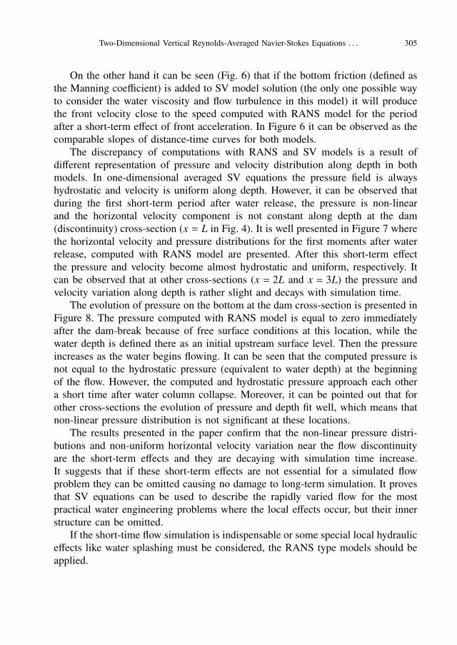
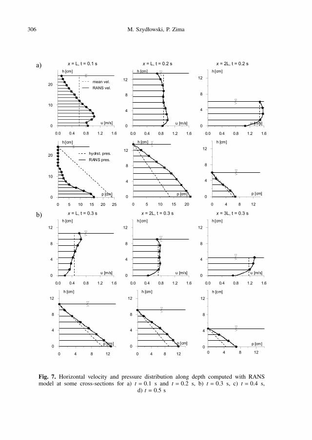
The discrepancy of computations with RANS and SV models is a result ofdifferent representation of pressure and velocity distribution along depth in bothmodels. In one-dimensional averaged SV equations the pressure field is alwayshydrostatic and velocity is uniform along depth. However, it can be observed thatduring the first short-term period after water release, the pressure is non-linearand the horizontal velocity component is not constant along depth at the dam(discontinuity) cross-section (x = L in Fig. 4). It is well presented in Figure 7 wherethe horizontal velocity and pressure distributions for the first moments after waterrelease, computed with RANS model are presented. After this short-term effectthe pressure and velocity become almost hydrostatic and uniform, respectively. Itcan be observed that at other cross-sections (x = 2L and x = 3L) the pressure andvelocity variation along depth is rather slight and decays with simulation time.

The evolution of pressure on the bottom at the dam cross-section is presented inFigure 8. The pressure computed with RANS model is equal to zero immediatelyafter the dam-break because of free surface conditions at this location, while thewater depth is defined there as an initial upstream surface level. Then the pressureincreases as the water begins flowing. It can be seen that the computed pressure isnot equal to the hydrostatic pressure (equivalent to water depth) at the beginningof the flow. However, the computed and hydrostatic pressure approach each othera short time after water column collapse. Moreover, it can be pointed out that forother cross-sections the evolution of pressure and depth fit well, which means thatnon-linear pressure distribution is not significant at these locations.

The results presented in the paper confirm that the non-linear pressure distri-butions and non-uniform horizontal velocity variation near the flow discontinuityare the short-term effects and they are decaying with simulation time increase.It suggests that if these short-term effects are not essential for a simulated flowproblem they can be omitted causing no damage to long-term simulation. It provesthat SV equations can be used to describe the rapidly varied flow for the mostpractical water engineering problems where the local effects occur, but their innerstructure can be omitted.

If the short-time flow simulation is indispensable or some special local hydrauliceffects like water splashing must be considered, the RANS type models should beapplied.


Fig. 7. Horizontal velocity and pressure distribution along depth computed with RANSmodel at some cross-sections for a) t = 0.1 s and t = 0.2 s, b) t = 0.3 s, c) t = 0.4 s,

d) t = 0.5 s


Fig. 7. (continued) Horizontal velocity and pressure distribution along depth computed withRANS model at some cross-sections for a) t = 0.1 s and t = 0.2 s, b) t = 0.3 s, c) t = 0.4 s,

d) t = 0.5 s


Fig. 8. Pressure (•) and depth (–) evolution at a) x = L (dam cross-section), b) x = 2L,c) x = 3L

6. Summary and Conclusions

In the paper, rapidly varied open channel flow due to dam-break effect was analysed.The analysis was based on experimental (Koshizuka et al 1995) and numerical in-vestigation of the water column collapse problem. In order to calculate the evolutionof flow parameters two mathematical models were used – RANS and SV equations.

Concluding, it should be pointed out that SV model (assuming hydrostaticpressure and uniform velocity distribution along water depth) is not an adequatedescription of flow near the local hydraulic effects (i.e. steep wave fronts, hy-draulic jumps, etc.). The better simulation results for short-term problems can beensured using RANS equations. Unfortunately, this model is too complex (even inthe two-dimensional vertical plane) to be applied for practical, free surface waterengineering problems. Therefore, SV equations still remain the main mathematicalmodel of open channel rapidly varied flow ensuring sufficiently good simulation re-sults for long-term typical engineering application problems where inner structureof local hydraulic effects and short-term pressure and velocity distribution evolutioncan be neglected. However, if the detailed description of flow parameters of localhydraulic effect is necessary, the RANS type models must be used.

Acknowledgment

The authors wish to acknowledge the financial support offered by Polish Ministryof Education and Science for the research project 2 P06S 034 29.

ReferencesAbbott M. B. (1979), Computational Hydraulics: Elements of the Theory of Free-Surface Flows,

Pitman, London.Anderson J. D. (1995), Computational Fluid Dynamics, McGraw-Hill Inc., New York.Bermudez A., Vazquez M. E. (1994), Upwind methods for hyperbolic conservation laws with source

terms, Computers and Fluids, 23, 1049–1071.


Cunge J. A., Holly Jr F. M., Verwey A. (1980), Practical Aspects of Computational River Hydraulics,Pitman, London.

Fletcher C. A. J. (1991), Computational Techniques for Fluid Dynamics 1. Fundamental and GeneralTechniques, Springer-Verlag, Berlin.

Granatowicz J., Szymkiewicz R. (1989), A comparison of the solution effectiveness of theSaint-Venant equations with finite element method and finite difference method, Archives ofHydro-Engineering and Environmental Mechanics, Vol. 36, No. 3–4, 199–210 (in Polish).

Koshizuka S., Tamako H., Oka Y. (1995), A Particle Method for Incompressible Viscous Flow withFluid Fragmentation, Computational Fluid Dynamics Journal, Vol. 4, No. 1, 29–46.

LeVeque R. J. (2002), Finite Volume Method for Hyperbolic Problems, Cambridge University Press,New York.

Maronnier V., Picasso M., Rappaz J. (1999), Numerical simulation of free surface flows, Journal ofComputational Physics, Vol. 155, 439–455.

Mohapatra P. K., Eswaran V., Bhallamudi S. M. (1999), Two-dimensional analysis of dam-break flowin vertical plane, Journal of Hydraulic Engineering, Vol. 25, No. 2, 183–192.

Morris M. W. (editor) (2000), Final Report – Concerted Action on Dam-break Modelling, HR Walling-ford Ltd., Wallingford.

Potter D. (1982), Computational Physics, PWN, Warsaw (in Polish).Remson I., Hornberger G., Molz F. (1971), Numerical Methods in Subsurface Hydrology, Wiley and

Sons, New York.Ritter A. (1892), Die Fortplanzung der Wasserwellen, Zeitschrift des Vereines Deutscher Ingeniere,

33(36), 947–954.Roe P. L. (1981), Approximate Riemann solvers, parameters vectors and difference schemes, Journal

of Computational Physics, Vol. 43, 357–372.Sawicki J. (1998), Free Surface Flows, PWN, Warsaw (in Polish).Szydłowski M. (editor) (2003), Mathematical Modelling of Dam-break Hydraulic Effects, Monographs

of Water Management Committee of Polish Academy of Science, Vol. 22, Warsaw (in Polish).Szydłowski M. (2004), Implicit versus explicit finite volume schemes for extreme, free surface water

flow modelling, Archives of Hydro-Engineering and Environmental Mechanics, Vol. 51, No. 3,287–303.

Szymkiewicz R. (2000), Mathematical Modelling of Open Channel Flows, PWN, Warsaw (in Polish).Toro E. F. (1997), Riemann Solvers and Numerical Methods for Fluid Dynamics, Springer-Verlag,

Berlin.Welch J. E., Harlow F. H., Shannon J. P., Daly B. J. (1966), The MAC Method, Technical Report

La-3425, Los Alamos National Laboratory.Zima P. (2005), The numerical simulation of two-dimensional vertical incompressible viscous flow,

[in:] Proceedings of Water Management and Hydraulic Engineering Ninth International Sympo-sium, Ottenstein-Austria, Sept. 4–7 2005, eds. H. P. Nachtnebel, C. J. Jugovic, Vienna, BOKU,Univ. Natural Resour. a. Appl. Sci., 455–462.

Zoppou C., Roberts S. (2003), Explicit schemes for dam-break simulations, Journal of HydraulicEngineering, Vol. 129, No. 1, 11–34.

Zwart P. J., Raithby G. D., Raw M. J. (1999), The integrated space-time finite volume method and itsapplication to moving boundary problems, Journal of Computational Physics, Vol. 154, 497–519.

Documents

Two-Dimensional Vertical Reynolds-Averaged Navier-Stokes · PDF fileTwo-Dimensional Vertical Reynolds-Averaged Navier-Stokes Equations Versus One-Dimensional Saint-Venant Model for