Embed Size (px)
Citation preview
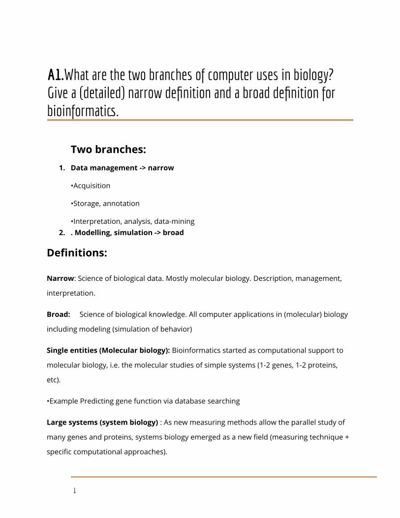
A1.What are the two branches of computer uses in biology? Give a (detailed) narrow definition and a broad definition for bioinformatics.
Two branches:1. Data management -> narrow
•Acquisition
•Storage, annotation
•Interpretation, analysis, data-mining2. . Modelling, simulation -> broad
Definitions:
Narrow: Science of biological data. Mostly molecular biology. Description, management,
interpretation.
Broad: Science of biological knowledge. All computer applications in (molecular) biology
including modeling (simulation of behavior)
Single entities (Molecular biology): Bioinformatics started as computational support to
molecular biology, i.e. the molecular studies of simple systems (1-2 genes, 1-2 proteins,
etc).
•Example Predicting gene function via database searching
Large systems (system biology) : As new measuring methods allow the parallel study of
many genes and proteins, systems biology emerged as a new field (measuring technique +
specific computational approaches).
1

•Example: Studying gene expression in a whole genome using next generation sequencing
A2. Give a generalized description of structures as entities and relationships-examples for entities and relationships in various systems!
System Entities Relationships
a) conceptual models of natural systems
Molecules Atoms atomic interactions/chemical bonds
Assemblies Proteins, DNA molecular contacts
Pathways Enzymes Chemical reactions
Genetic networks Genes Co-regulation
b) structural descriptions
Protein structure Atoms Chemical bonds
Protein structure Secondary structures Sequential and topological vicinity
Folds Calpha atoms Peptide bond
Protein sequence Amino acid Sequential vicinity
Structure definitions are hierarchical (atom – amino acid – protein – pathway – cell – tissue
etc.) For a given problem it is convenient to choose a standard description or “core
structural level”. E.g. DNA sequences are the standard level for molecular biology problems.
For a standard or core description, we always have an underlying logical structure, plus
various additional, simplified and annotated views. (annotation means extending with
external information).
2

Structure is a (~constant space-time) arrangement of elements or properties. Function is a
role played within a system.
A3.Describe the core data-types used in bioinformatics! Name the underlying models, the principal form of description and give examples of extended and simplified descriptions(annotations)!
Sequences
Logical structure: Chemical formula (series of amino acids
or nucleotides)
Standard description: Series of characters :IFPPVPGP
Simplified and/or extended visualization: DNA binding and
signal binding regions marked on the pic
3D structures
Logical structure: 3D chemical structures
Standard description: 3D coordinates + subunit descriptions (atomic,
amino acid, nucleotide)-(xi, yi, zi)n
Simplified and/or extended (annotated) visualization: kis ábra hogy mit hol köt meg
ilyenek
Networks
Logical structure: entities, relationships
3

Standard description: Graphs
Simplified and/or extended (annotated) visualization: másik kis ábra ahol a gárfon be
vannak jelölve a dolgok, pl: signal synthesis, signal transduction
Texts
Human messages written in scientific language.
Like other data, they have logical structure, standard, simplified and extended descriptions
and databases. BUT: messages have an emitter (author) and an audience (reader,
reviewer). In other words they are context dependent (unlike, say, sequences or atoms)
Loosely structured (not as well as molecules). There are ontologies for the language but
not for the articles themselves!
Title, abstract -simplified descriptors
QUESTION-> introduction
ANSWER-> results, methods -standard description
CONCLUSIONS-> discussion
references, keywords- annotations
Sequences resemble languages („language metaphor”)
3D structures resemble real life objects („object metaphore”)
Networks resemble social asemblies („social metaphore”)
Scientific papers are messages (”communication metaphor”)
4

5

A4. Give a short overview of data representation types (structured, unstructured, mixed), and what is granularity!
Predictive models can use any property (unstructured descriptions). For exact prediction,
“information richness” is important, not the exact meaning of the variables
For interpretative models, the content should be as simple as possible, but the meaning is
important (as structured as possible)
Types: unstructured and structured (depending if we know or want to use the internal
structure)
Granularity: resolution of the description (e.g. 4 nucleootides, 16 dinucleotides)
Unstructured representations
•We know nothing about internal structure
•Only the properties are known (global descriptors), can be discreet
or continuous.
•Best described as vectors (each dimension is an attribute, the
contents is the value..). Sometimes a large number of dimensions.
•Vector operations are fast(real valued vectors)
Here we use the EAV terminology.
(AV)n -> binary/real valued vectors
Vector types:
6

Binary vectors consist of 0 or 1 values, e.g. 0,1,0,0,1,0. Indicate the presence or absence of
attributes.
Non-binary vectors can contain real or integer-valued components, e.g., 0.5, 0.9, 1.0.
Structured representation
•We know the internal structure in terms or Entities and
Relationships (both described in terms of attributes and values ->
EAV and “RAV”)
•Information-rich, allows detailed comparisons.
•Need alignment (matching) for comparison…
•Examples: character strings (sequences), graphs (most molecular structures are like this..)
(EAV)m (RAV)n->graphs
Mixed or composition-like descriptions
•We decompose an object to parts of known structure, and
count the parts (atomic composition, H2O, or amino acid
composition of proteins).
•The result is a vector, fast operations, alignment (matching) is
not necessary
•The information content of the vector depends on the
granularity of the parts. Atomic composition of proteins or of people is not informative.
(EAV)n -> vectors (binary/real valued)
7

Granularity:
Granularity is the resolution of a description (e.g. of a vector)
Too high resolution: all objects seem to be different, no similarity between members of the
same group...
Too low resolution: All objects are equal, no difference between different groups
Finding the right amount of detail is hard. This is part of „the curse of dimensionality”
At low dimensions, all sequences are similar. At very high ones all are different…
8

For a given problem, you can find an optimal resolution. Say you want to find the optimal
granularity to separate two sequence groups, using word vectors (one of the groups can be
very large a random selected group).
You can calculate all distances within the groups and between the groups.
You can compare the two distance sets with standard statistics, such as a t-test etc.
You do this for all resolutions, and see - from a plot - if there is one which is more
significant than the other.
This is true of course only for normal distributions, but we can suppose that the bias will be
the same for all points on the plot.
9

A5. What are the substitution matrices? Describe PAM and Blosum matrices!
Substitution matrices in details
The susbstitution matrix (also called scoring matrix) contains costs for amino acid
identities and substitutions in an alignment.
For amino acids, it is a 20x20 symmetrical matrix that can be constructed from pairwise
alignments of related sequences
“Related” means either :
● evolutionary relatedness described by an “approved” evolutionary tree (Dayhoff’s
PAM matrices)
● any sequence similarity as described in the PROSITE database (Hennikoff’s BLOSUM
matrices)
Groups of related sequences can be organized into a multiple alignment for calculation of
the matrix elements.
Matrix elements are calculated from the observed and
expected frequencies (using a “log odds” principle).
PAM matrices
Percent Accepted Mutation: Unit of evolutionary change
for protein sequences [Margaret Dayhoff78].
10

Calculated from related sequences organized into “accepted” evolutionary trees (71 trees,
1572 exchange [only])
Derived from manual alignments of closely related small proteins with ~15% divergence.
20x20 matrix, columns add up to the no of cases observed.
Converted into scoring matrix by log-odds and scaling.
Pam_1 = 1% of amino acids mutate
Pam_30 = (Pam_1)^30 (matrix multiplication)
First useful scoring matrix for protein
Assumed a Markov Model of evolution (I.e. all sites equally mutable and independent)
Higher PAM numbers to detect more remote sequence similarities
Lower PAM numbers to detect high similarities
1 PAM ~ 1 million years of divergence
Errors in PAM 1 are scaled 250X in PAM 250
PAM 40 - prepared by multiplying PAM 1 by itself a total of 40 times, best for short
alignments with high similarity
PAM 120 - prepared by multiplying PAM 1 by itself a total of 120 times, best for general
alignment
PAM 250 - prepared by multiplying PAM 1 by itself a total of 250 times, best for detecting
distant sequence similarity
11

BLOSUM Matrices (most often used)
Developed by Henikoff & Henikoff (1992)
BLOcks SUbstitution Matrix
Derived from the BLOCKS database
Much later entry to matrix “sweepstakes”
No evolutionary model is assumed
Built from PROSITE derived sequence blocks
Uses much larger, more diverse set of protein sequences (30% - 90% ID)
Lower BLOSUM numbers to detect more remote sequence similarities
Higher BLOSUM numbers to detect high similarities
Sensitive to structural and functional substitution
Errors in BLOSUM arise from errors in alignment
BLOSUM 90 - prepared from BLOCKS sequences with >90% sequence ID
best for short alignments with high similarity
BLOSUM 62 - prepared from BLOCKS sequences with >62% sequence ID
best for general alignment (default)
BLOSUM 30 - prepared from BLOCKS sequences with >30% sequence ID
best for detecting weak local alignments
12

13

A6. What types of alignments exist according to what we compare with what? Give examples for the usage of each method!
We usually compare one unknown sequence or less known sequence, the “query”, with a
known sequence, the “subject” or the “database entry”.
We can now classify the alignment problems according to what the query is and what the
subject or entry is.
What is the technical difference between the various heuristic algorithms? Mostly,
a) the how we reduce the search space to a manageable size (choosing a good
representation, clever memory management and searching schemes), and
b) the way how we calculate the random distribution (for the significance calculation).
What do we align?
1) Two gene/protein sequences (basic exercise)
One-to-one: Pairwise alignment (approximate string matching)
Goal: finding the best alignment.
If resources allow it, we use exhaustive algorithms.
For a single pair we also use visual evaluation by dot plot, sequence plots
(hydrophobicity, etc.)
14

2) One gene/protein seq vs a database of many gene/protein seq.s: DATABASE
SEARCHING
Usually called database searching. Many pairwise alignments (approximate string
matching). One-to-many.
Goal: finding the best matching item (eg. sorting by score).
Single gene/protein analysis. Exhaustive alignments are usually too time consuming.
GPU methods now make them possible...
Rather, we use heuristics to restrict exhaustive alignment to a few sequences and to
shorter regions… (e.g. BLAST).
3) Many short DNA seq.s vs one long DNA seq e.g. genome. (IDENTIFYING
MUTATIONS)
Genome sequencing. Short seq.s can be expressed sequence tags, sequence reads
from shotgun sequencing etc. Short seq.s are highly redundant and noisy (contain
random mistakes, truncations etc.). Many-to-one.
Goal: finding the best matching regions. Many short seq.s can match the same
region. Exhaustive alignment is too time/resource intensive.
Heuristics necessary to reduce search place BLAT, BWA. These heuristics are
different from BLAST.
4) Many very short seq.s vs. many very short seq’s ( 1) DIAGNOSING KNOWN DISEASE
MUTATIONS IN SELECTED HUMAN GENES, BACTERIAL METAGENOMICS)
Targeted resequencing (diagnostic tasks…). Many-to-one (a few or few hundred
times).
15
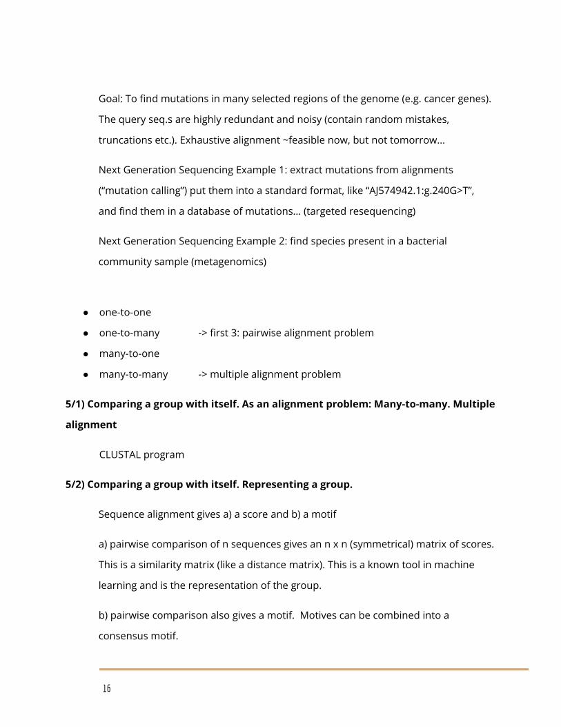
Goal: To find mutations in many selected regions of the genome (e.g. cancer genes).
The query seq.s are highly redundant and noisy (contain random mistakes,
truncations etc.). Exhaustive alignment ~feasible now, but not tomorrow…
Next Generation Sequencing Example 1: extract mutations from alignments
(“mutation calling”) put them into a standard format, like “AJ574942.1:g.240G>T”,
and find them in a database of mutations… (targeted resequencing)
Next Generation Sequencing Example 2: find species present in a bacterial
community sample (metagenomics)
● one-to-one
● one-to-many -> first 3: pairwise alignment problem
● many-to-one
● many-to-many -> multiple alignment problem
5/1) Comparing a group with itself. As an alignment problem: Many-to-many. Multiple
alignment
CLUSTAL program
5/2) Comparing a group with itself. Representing a group.
Sequence alignment gives a) a score and b) a motif
a) pairwise comparison of n sequences gives an n x n (symmetrical) matrix of scores.
This is a similarity matrix (like a distance matrix). This is a known tool in machine
learning and is the representation of the group.
b) pairwise comparison also gives a motif. Motives can be combined into a
consensus motif.
16

A (G or C)AA(any nucleotide x 5)T -> regular expression etc.
This is another important representation of the group.
17

A7. Describe pairwise and multiple alignments! Give the relationship between pairwise and multiple alignment (difference in complexity and its consequences, construction of pairwise from multiple alignment and multiple from pairwise alignment)!
(EZT INNENTŐL NEM TUDOM HONNAN SZEDTEM MOST HIRTELEN-
The input of a sequence alignment algorithm:
1) Two sequences
2) A scoring scheme (a score formula AND a scoring (substitution) matrix)*
*This is applicable also to the comparison of 3D structures of macromolecules, or any other type of linear object descriptions
The steps of sequence alignment:
1) Find all possible alignments (Mappings) between two sequences and find the best according to some “quick” score.
2) Calculate a final quantitative score for the best alignment (Matching)
The results of sequence alignment:
1) A score (similarity score or distance)
2) A motif (common substructure, consensus description…)
Score =
(Gap) penalty =
18

Gap penalty functions:
Linear: Penalty rises monotonous with length of gap
Affine: Penalty has a gap-opening and a separate length component
Probabilistic: Penalties may depend upon the neighboring residues
Other functions: Penalty first rises fast, but levels off at greater length values
The alignment algorithms themselves are in: B4
What methods to select according to the time/resources we have?
If we have time/resources, we can try exhaustive algorithms. This is an option with
supercomputers or GPU implementations…
For realistic problems (and realistic resources) we need heuristic alignments that restrict
the search space to a manageable size…. at a price of loosing some accuracy.
● Alignments can be exhaustive or heuristic
Exhaustive, also called dynamic programming, if we do not need much of resources
(e.g. we have few sequences to align)
Heuristic, for realistic problems where time is an issue
● Alignments can be global and local
Global: from beginning to end
Local: pinpoint highly similar regions (more realistic)
-IDÁIG DE EZ IS BIZTOS KELL VALAHOVA )
19

What is a multiple alignment
•A method to visualize a group of sequences. A group description.
•A group of similar sequences has two main representations:
A similarity group -> multiple alignment
-> tree
Why not exhaustive algorithms?
•In the previous lectures we heard that exhaustive, dynamic programming algorithm
can be used to align TWO sequences
•Smith Waterman for local alignment, and Needleman Wunsch for global alignment.
•Since we analyze short sites or single domain proteins Needleman Wunsch is often
used...
From Pairwise To Multiple
•A multiple alignment can be
decomposed into to pairwise
alignments.
•Delete all lines but two and then
delete all columns that are empty
(contain only gaps).
•This pairwise alignment will still contain the “traces” of the multiple alignment: A
simple pairwise alignment algorithm may give a different result.
20

•A multiple alignment can not always be constructed from pairwise alignments.
•Mathematicians say there are sequences that can not be well aligned
•Engineers know that these strange cases are those that should never be aligned, to
start with…. (slide 6)
Additive approach(“once a gap, always a gap”)
•Do all pairwise alignments (e.g. Needleman Wunsch)
•Select a simple, ADDITIVE representation for the alignments:
•For instance: Sequence A in alignment X can be represented as a series of gaps at
given positions (pos 4, 5; pos 5: 1). This is a sparse vector.
•Such representations can be added. Sequence A in the multiple alignment will
contain the max amount of gaps at each position. This is a special case of vector
addition.
•After constructing the multiple alignment in such a way, we need to remove all
columns that contain only gaps.
21
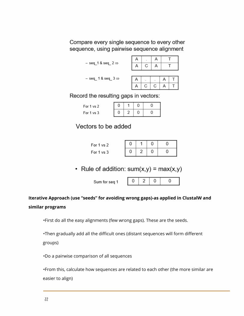
Iterative Approach (use “seeds” for avoiding wrong gaps)-as applied in ClustalW and
similar programs
•First do all the easy alignments (few wrong gaps). These are the seeds.
•Then gradually add all the difficult ones (distant sequences will form different
groups)
•Do a pairwise comparison of all sequences
•From this, calculate how sequences are related to each other (the more similar are
easier to align)
22

•Perform multiple alignment in order; the most similar are aligned first, the others
are saved for later
1: Pairwise Comparison: Compare every single sequence to every other sequence,
using pairwise sequence alignment, record the resulting similarity scores
2: Calculate the guide tree: Construct a guide tree from the matrix containing the
pairwise comparison values, using a clustering algorithm –Neighbor-Joining (Clustal
W)
3: Multiple Alignment: Using the guide tree, we start aligning groups of sequences,
the purpose of the guide tree is to know which sequences are most alike; so we can
align the “easy” ones first, and postpone the tricky ones to later in the procedure!
The most similar sequences give the “seeds”, CLUSTAL combines the seeds.
What are alignments good for?
-An alignment built from a group can be used to find new members of the group –
this is a more sensitive comparison than sequence alignment…The tools are Profiles
and HMMs (see a later lecture!)
-Alignments libraries for interesting sequence groups like protein domain types…
(today there are ~12,000 types). Searching such small collections is possible with
exhaustive algorithms, in short times. Predicting the functions in new sequences
(genome annotation).
-One can align MAs – this is the most sensitive comparison for sequences today…
Practical use 1. highlighting conserved positions in a Multiple Alignment: Conserved
positions are the essence of a multiple alignment
23

Practical use 2. constructing a consensus sequence from conserved positions
Practical use 3. constructing a regular expression from conserved positions
24

A8. Protein groups are heterogeneous from a number of points
of view. Name a few group properties that make protein
classification difficult! Explain the role of within - group and
between - group similarities!
25

B1. Describe data comparison-score, common alignment patterns!
Understanding data: grouping and classifying, organizing into knowledge items, matching to
other knowledge items.
Humans operate on “logical structures”. Computers operate on descriptions (which are
given to them by humans).
Similarity by structure: similarity groups/neighbourhoods, multiple alignments, evolutionary
trees
Similarity by context/function: metabolic pathways, subunits, ligands,
genomes, trajectories
Patterns are more than the sum of their parts. The emergence of
new patterns is not explained by the traditional, structuralist
approach
Similarity by Humans and Machines
Humans use intuitive patterns, and similarity is defined as a shared pattern (motif). AFTER
that we also use scores
Patterns are either instinctive or knowledge based
The choice and form of the patterns is flexible
26

Consensus patterns are in the memory, validated and updated by experience
->Flexible, qualitative
Computers use descriptions (vectors, character strings) and a) compute numerical
similarity measures („scores”), b) search for predefined patterns
Descriptions, numerical measures and patterns are all predefined
Scores and motifs are validated by statistics (significance, predefined algorithms)
Memory: dbases
-> Rigid. quantitative
A “representation”
•Entities are described by the EAV scheme (entity, attribute, value). E.g. apple has an
attribute “weight”, its value is 150 g. Protein X has a molecular weight of 100,000 daltons
•Relations are described in the same way: A single chemical bond has an attribute “length”
which is 1.4 Angstroms. Here we call this a RAV (relation, attribute, value) scheme.
•A “structure” is a structured set of encapsulated EAV substructures
Comparison
Input: Two descriptions
Output:
- For unstructured: a score (similarity, distance), mandatory
- For structured: a score (like above, mandatory ) AND a common pattern (result of
matching=alignment), optional
Proximity measures (scores)
27

•Similarity measures (zero for different objects, large for identical objects)
•Distances (large different objects, zero for identical objects)
•Exist both for vectors and for structures…
•“Well behaved”: if bounded, e.g. [0,1]
•Don’t expect linearity in any sense… (“twice as similar” makes no sense)
•Similarity S~1/D or 1-k*D..
Vector distances
•The concept of proximity is based on the concept of distance.
•The most popular distance of two points, a and b in the plane is the euclidean distance:
(ez itt a gyök alatt van )
Metric properties:
1. Distance is positive Dab >= 0,
2. Distance from oneself is zero, Daa =0.
3. Distance is the same in both directions, Dab= Dba
4. Triangular inequality Dab + Dbc > Dac
Generalized Distances
•The concept of distance can be extended to n
dimensions:
28

•AND it can be extended to exponents other than 2
Similarity measures for vectors
•The dot product or inner product of two vectors is by
defined:
•For binary vectors (dimensions zero or one) this is the number of matching nonzero
attributes.
• Vectors of unit length have a dot product [0,1], 1.0 for identical vectors
Association measures
•Association measures are typically used to measure the similarity
between binary (“presence-absence”) descriptions (property sets).
The Jaccard (or Tanimoto) coefficient [0,1] expresses the similarity
of two property sets a and b of non-zero attributes, respectively as:
A remark on proximity measures
•There is a very large and ever growing number of proximity measures.
•For easy problems, many of them work equally well… For difficult problems none of them
do.
Comparing structured descriptions
•Input: 2 structured descriptions (say, sequences)
•Output: 1) a proximity measure (score) and 2) a shared pattern (motif).
29

•You can use proximity measures if you can turn the description into a vector (see
composition-type description).
•In addition, you can match (align) structures that gives a shared pattern.
Matching (general) structures: Matching graphs consists of finding the largest common
subgraph. A computationally hard problem. Finding approximately identical subgraphs is
NP complete. In the human mind, matching is instinctive (comparing cars…)
Matching bit or character-strings, Hamming distance: The Hamming distance is the number of
exchanges necessary to turn one string of bits or characters into another one (the number
of positions not connected with a straight line). The two strings are of identical length and
no alignment is done.
The exchanges in character strings can have different costs, stored in a lookup table. In this
case the value of the Hamming distance will be the sum of costs, rather than the number of
the exchanges
Edit distance between character strings (sequences), Levenshtein distance: Defined as a sum of
costs assigned to matches, replacements and gaps (= insertions and deletions). The two
strings do not need to be of the same length. A numerical similarity measure between
biological sequences is a maximum value calculated within a range of alignment. The
maximum depends on the scoring system that includes 1) a lookup table of costs, such as
the Blosum matrix for amino acids, and 2) the costing of the gaps. The scores are often not
metric, but closed to metricity…
Motif between aligned sequences: Shared motifs point to evolutionary conservation. More
informative than simple sequences. „What a sequence whispers, an alignment pattern
shouts out loud”
30

Significance of a similarity score
31

B2. Give a short overview of the statistics of alignments (e-value, p-value, z-score, linearization, Karlin-Altschul statistics)!
Significance:
1) The probability of finding a score by chance (p-value) ;
2) The number of times you expect to find a score >= a certain value by chance (E-value,
expect value). (the smaller, the better – true for both)
You can estimate p by making a histogram of chance (random) scores, linearizing it and
reading p from the linear curve.
This area is the p-value
The p-value is the probability of
observing data at least as
extreme as that observed.
Methods to estimate significance differ in how they model the distribution of random
scores (DRS)
a) Calculation of score by simulating DRS with random shuffled sequences (Z-score).
Applicable to a single alignment…
b) Comparison with a histogram of unrelated similarity scores (using either a random db or
the low (approximately random) scores of the real data.
32

b1) Without knowing the distribution (linearization and reading from the curve)
b2) Determining the distribution (like the extreme value distribution of the Karlin-
Altschul statistics, see later at the BLAST program)
Karlin-Altschul: local alignment without gaps
The Z-score: Calculating significance for comparing two sequences, A and B.
First calculate score comparing A and B (this is the “genuine score”, Sgenuine)
Then repeat N times (N > 100):
● Randomise sequence A by shuffling its residues in a random fashion (This will be the
“random database”)
● Align randomised sequence A to sequence B, and calculate alignment score
Srandom
Calculate mean Ŝrandom and standard deviation σrandom
Calculate Z-score: Z = (Sgenuine – Ŝrandom) / σrandom
Z-score statistics – why not to use it:
Z-score implies a normal distribution of scores – this is NOT true!
Shuffling sequence A will give sequences with the same composition as A…. (other
compositions are not considered)
Biased sequences, like AAAAAAAAA remain the same at randomization so σrandom will be
close to zero…
Natural sequences are NOT like random shuffled ones, some dipeptides, tripeptides (and
~nucleotides) are more frequent than others.
33

Calculating Z-scores for all alignment pairs during database searches (i.e. for one million
alignments) is not practical – Takes too long.
b1) Estimating significance from an unknown distribution
34

Where to get the distribution of random (chance) similarities?:
a) comparison with real sequences, omitting largest scores.
b) Using many, different simulated, random-shuffled sequences. Neither is “correct”
but both work quite well
Usually one has to extrapolate quite far since large S values are rare (red line)… True, but
there is no other way.
35

B3. Explain the Dot Plot method! Write down the algorithm, describe the parameters and list some usages!
Graphical comparison of sequences using “Dotplots”.
Basic Principles:
1) Write sequences of length n on two diagonal axes. This defines an n x n matrix, called
the dot matrix or alignment matrix.
2) Imagine that we put now a red dot to those positions where the nucleotides x(i) and y(i)
are identical.
3) If the two sequences are identical, the diagonal will be red. x(i) = y(i) all along the
sequences
4) If 10 nucleotides are deleted in sequence y at a certain position, but the two are
otherwise identical, then after the point of deletion y(i) = x(I +10)
We can view this two ways:
y(i) = x(i +10) insertion in x or y(i-10) = x(i) deletion in y
Scoring schemes
DNA: Simplest Scheme is the Identity Matrix, more complex matrices can be used.
The use of negative numbers is only pertinent when these matrices are used for computing
textual alignments.
36

Using a wider spread of scores eases the expansion of the scoring matrix to sensibly
include ambiguity codes.
For Protein sequence dotplots more complex scoring schemes are required.
Scores must reflect far more than alphabetic identity.
Faster plots for perfect matches:
To detect perfectly matching words, a dotplot program has a choice of strategies1. Select a scoring scheme and a word size (11, say)
For every pair of words, compute a word match score in the normal way
- only if the maximum cut- off score is achieved(11)- celebrate with a dot
- if the possible maximum cut- off score is still not achieved- do not celebrate
with a dot
2. For every pair of words:
- see if the letters are exactly the same- celebrate with a dot
- if they are not- do not celebrate with a dot
To detect exactly matching words, fast character string matching can replace laborious
computation of match scores to be compared with a cut-off score Many packages include a
dotplot option specifically for detecting exactly matching words.
Particular advantage when seeking strong matches in long DNA sequences.
Dotplot parameters:
1)The scoring scheme:
DNA: Usually, DNA Scoring schemes award a fixed reward for each matched
pair of bases and a fixed penalty for each mismatched pair of bases.
Choosing between such scoring schemes will affect only the choice of a
sensible cut-off score and the way ambiguity codes are treated.
37
Protein: Protein scoring schemes differ in the evolution distance assumed between
the proteins being compared. The choice is rarely crucial for dotplot programs.
2)The cut-off score
The higher the cut-off score the less dots will be plotted.
But, each dot is more likely to be significant.
The lower the cut-off score the more dots will be plotted.
But, dots are more likely to indicate a chance match (noise).
3)The word size
Large words can miss small matches. Smaller words pick up smaller features. The smallest
“features” are often just “noise”.
For sequence with regions of small matching features- small words pick up small features
individually. Larger words show matching regions more clearly. The lack of detail can be an
advantage.
Other uses of dotplot :
Detection of Repeats: ugyanaz a szekvencia felvitele mindkét tengelyre
Detection of Stem Loops: ugyanaz a szekvencia felvitele mindkét tengelyre, majd az egyik
megfordítása
38

B4. What is the difference between global and local alignment? Explain the main algorithms (Needleman&Wunsch and Smith&Waterman), and gap-handling!
Pairwise alignment – the simplest case
We have two (protein or DNA) sequences originating from a common ancestor.
The purpose of an alignment is to line up all positions that originate from the same
position in the ancestral sequence. The purpose of an alignment is to line up all residues
that were derived from the same residue position in the ancestral gene or protein in two
sequences.
Global alignment
Align two sequences from “head to toe”, i.e. from 5’ ends to 3’ ends from N-termini to C-
termini.
Exhaustive algorithm published by: Needleman, S.B. and Wunsch, C.D. (1970)
“A general method applicable to the search for similarities in the amino acid sequence of
two proteins” J. Mol. Biol. 48:443-453.
“Exhaustive” means: all cases tested so the result (the alignment) is guaranteed to be
optimal.
Simple rules:
–Match (i,j) = 1, if residue (i) = residue (j); else 0
–Gap = 1
–Score (i,j) = Maximum of:
39

•Score (i+1,j+1) + Match (i,j)
•Score (i+1,j) + Match (i,j) - Gap
•Score (i,j+1) + Match (i,j) - Gap
Advanced rules:
–Match (i,j) =•W(i,j), where W is a score matrix, like PAM250
–Gap =Gap_init + Gap_length x length_of_gap
–Score (i,j) = Maximum of:
•Score (i+1,j+1) + Match (i,j)
•Score (i+1,j) + Match (i,j) - Gap
•Score (i,j+1) + Match (i,j) - Gap
Local alignment
Locate region(s) with high degree of similarity in two sequences
Exhaustive algorithm published by: Smith, T.F. and Waterman, M.S. (1981)
“Identification of common molecular subsequences” J. Mol. Biol. 147:195-197.
Simple rules:
– Match (i,j) = 1, if residue (i) = residue (j); else 0
–Gap = 1
–Score (i,j) = Maximum of:
•Score (i+1,j+1) + Match (i,j)
•Score (i+1,j) + Match (i,j) - Gap
•Score (i,j+1) + Match (i,j) - Gap
•0
Advanced rules:
–Match (i,j) = W(i,j), where W is a score matrix, like PAM250
40

–Gap = Gap_init + Gap_length x length_of_gap
–Score (i,j) = Maximum of:
•Score (i+1,j+1) + Match (i,j)
•Score (i+1,j) + Match (i,j) - Gap
•Score (i,j+1) + Match (i,j) - Gap
•0
41

B5. What is the main idea of dynamic programming - example: multiple alignment of 3 sequences (additive approach)? Describe the principle of the ClustalW algorithm (iterative approach)!
Concepts of dynamic programming
Dynamic programming is a method for solving complex problems by breaking them down
into simpler subproblems
Solve the subproblems and combine the solution of the subproblems to reach an overall
solution
Solve each subproblem only once, store the result, and reuse it if needed later
Advantages :
● Solves mathematical and practical problems
● It can work with exponentially growing data
● Easy to optimize
● Run time is low (but higher memory usage)
● Opportunity to parallel running
Needleman-Wunsch algorithm
Dynamic programming solution to pairwise global alignment
Residues are aligned based on a scoring scheme that takes into account the evolutionary
relations
These scores can be summarized in a substitution matrix( like BLOSUM62)
We will also need a gap penalty but I this algorithm is detailed somewhere else
42
Smith- Waterman algorithm
Dynamic programming solution to pairwise local alignment
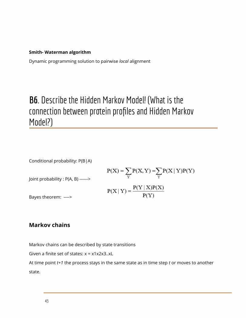
B6. Describe the Hidden Markov Model! (What is the connection between protein profiles and Hidden Markov Model?)
Conditional probability: P(B|A)
Joint probability : P(A, B) ------>
Bayes theorem: ---->
Markov chains
Markov chains can be described by state transitions
Given a finite set of states: x = x1x2x3..xL
At time point t+1 the process stays in the same state as in time step t or moves to another
state.
Transition probability: pij (the probability of moving from the ith state to the jth) we can
build a state transition matrix from them:
43

Markov property: next state depends only on the actual one:
The Markov chain above is able to generate random sequences
We need: beginning and end points
HMM - CpG islands
GC -rich,long region of DNA or
RNA (at least 200bp)
Being on an island: „+” symbol
Are we on a CpG island?
When we have a character series we can’t say which character comes from the island and
which is not, this makes the model „hidden”.
HMM- components
Hidden states (CpG island/loaded dice) and (observable) emitted symbols ({ACTG}/{ 1 , 2 , 3 ,
4 , 5 , 6 })
Output matrix: probability of observable symbols given that the hidden model is in a
certain hidden state
Initial distribution: the probability of the model being in a certain hidden state at time 0
State transition matrix : probability of moving from one hidden state to another hidden state
44

Viterbi algorithm
What is the most probable path? which series should we choose?
Most probable path:
Let Vk(i) be the probability that the most probable path ends at k. state where it emits
symbol xi
where ei(xi+1) is the probability of emitting xi+1 at the state l. , akl is the transition
probability from k to l
With dynamic programming we can get the most probable path:
Forward algorithm: estimates the probability of a sequence reading it forward
Backward algorithm: estimates the probability of a sequence reading it backward
Posterior decoding of the characters generated by the unfair casino. Y axis gives the
probability that the ith roll was made by normal dice.
45

Baum-Welch method
Usually we don’t know the parameters (transition and emission probabilities) of the HMM,
so we want to estimate them
Baum - Welch method: expectation maximalization
Algorithm:
● We start with random state series whose length matches
● The average length of the sequences (model)
● We align the sequences to the model
● We estimate the parameters (transition and emission probabilities)
● We calculate the state transition for the new parameters
● Iterate this as long as the model changes
Profile HMM
Given a protein family and we want to find other members of this family in a given
database.
We can make a profile that represents the protein family and we compare the database
elements to this profile. An HMM can describe such a profile
States:
M: match state
I: insertion state
46

D: deletion state (silent state – no emission)
n: length of sequence (number of matches)
47

B8. What is similarity searching in a database, what are the main steps, the importance of it, what kind of heuristics do you know?Given a query and a database, find the entry in the database that is most similar to the
query in terms of a numerical similarity measure (distance, similarity score, etc.)
(In contrast: retrieval looks for an exact match to the query.
Is John on the paylist? Retrieval: Yes/No, based on exact matching.
Similarity search: His brother Joe Brown is. So we classify John into the Brown family, based
on approximate matching.)
Steps of similarity searching
Starting stage: Query and DB are in the same format (the search format) and we have a
similarity measure.
1. Compare query with all entries in the DB and register similarity score. Store results
above some threshold (cutoff)
2. Calculate significance of the score (compared to chance similarities)
3. Rank entries according to similarity score or significance (top list)
4. Report the best hit (usually after some simple statistics, e.g. if it is higher than a
threshold…), add alignment pattern.
5. Assume function of query, i.e. classify query into a class present in the database.
Alignment pattern is a confirmatory proof for classification.
Important formulas
48
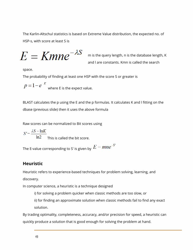
The Karlin-Altschul statistics is based on Extreme Value distribution, the expected no. of
HSP-s, with score at least S is
m is the query length, n is the database length, K
and l are constants. Kmn is called the search
space.
The probability of finding at least one HSP with the score S or greater is
where E is the expect value.
BLAST calculates the p using the E and the p formulas. It calculates K and l fitting on the
dbase (previous slide) then it uses the above formula
Raw scores can be normalized to Bit scores using
This is called the bit score.
The E-value corresponding to S' is given by
Heuristic
Heuristic refers to experience-based techniques for problem solving, learning, and
discovery.
In computer science, a heuristic is a technique designed
i) for solving a problem quicker when classic methods are too slow, or
ii) for finding an approximate solution when classic methods fail to find any exact
solution.
By trading optimality, completeness, accuracy, and/or precision for speed, a heuristic can
quickly produce a solution that is good enough for solving the problem at hand.
Search heuristics belong to i) i.e. they serve for reducing the search space.
49

We use a version of the edit distance and a specific substitution matrix (Dayhoff, BLOSUM,
etc.)
Why we need heuristics, and what kind…
•Exhaustive algorithms (Dynamic programming) are expensive,
•We use heuristics that make use of the properties of biological sequences (BLAST)
Computational heuristics:
a) exact matching is fast,
b) search space can be easily reduced.
Biological heuristics include
a) local similarities are dense,
b) similar regions are near each other,
c) low complexity sequences excluded, etc.
Computational heuristics I.- Word based methods
•Exact word matching is fast, use it whenever you can.
•Word composition vectors are a possibility but: word (n-gram) dimensionality grows fast
with word size
•Longer words are more informative but few of the possible words occur in a given
sequence, and most of them only once…
•We can make use of the longer words if we look only for shared (common) words. There
are much fewer of these…
•Potentially shared words are all the words of two sequences… (for two 100-amino acid
sequences, how many words of size 2 are in total?
•Word indexing methods, such as hash tables are extremely fast. But you need to build an
index (extra overhead).
Computational heuristics II.- Search space reduction
50

•Most sequences in a dbase are not similar to a given query. It is easy to construct filters
that throw away uninteresting sequences.
•Threshold based filtering is important, but has drawbacks (you can throw away important
hits)
•Two step workflows: Use fast methods to filter out most of the dbase entries, and use
increasingly expensive methods only for the important ones.
•Typical filter 1: Keep only sequences that contain n common words with the query.
•Typical filer 2: The shared words should be in the right distance. Or, they should be in the
right serial order.
Biological heuristics I. Search space reduction
•If you absolutely need dynamic programming, search only the vicinity of the diagonal
Biological heuristics II.- Short conserved sequences
•Sequence related by evolution always contain conserved regions that are highly similar,
contain rows of identical residues… Identify them during the calculation that do not and
omit them from the score….
•Danger: difficult to define, what is a conserved region (and what is a good threshold)
Biological heuristics III. - Repetitive or “low complexity” regions
•Biological sequences often contain repetitive of “biased composition”, “low complexity”
regions. These can be excluded from the query by masking them in advance with X-es in
order to omit them from the entire calculation
•Such sequences contain a biased composition of n-gram words, they are thus less
complex (can be described with fewer words).
•They give background noise since e.g. AAAAAA would match all sequences containing A-s.
51
•Such low-complexity regions should be excluded from the comparisons. The SEG program
of John Wootton masks them with X-es, before comparison.
Similarity searching today
•Genome sequences (especially microbes) are determined today by the thousands.
•Automated similarity searching (BLAST) is used to annotate their proteins by similarity.
Up to 40% of protein sequences (ORFs) are still unannotated. This usually includes the shell
genome, i.e. most of the specific functions, like toxicity, pathogenesis. The rest, i.e. the core
genome is always well known
What do we expect from heuristics?
•Should be 100-200 times faster than dynamic programming
•Should be able to find distant similarities between sequences related by evolution (e.g. in
new genomes).
•This is the goal of traditional heuristic search programs (FASTA, BLAST, BLAT, we now deal
only with BLAST).
•New fields, like medical diagnostics may require different heuristics.
52

B9. Describe BLAST algorithms in details! What kind of
heuristics does BLAST use? How can the BLAST specificity be
improved? List 5 different BLAST programs (query type)!
Blast: Basic Local Alignment Search Tool
Input: 1) query sequence 2) sequence dbase a) in preprocessed form [for fast screening] b)
in “normal” form for presenting the alignments using Smith-Waterman
Output: a) Toplist of most similar sequences, ranked according to significance (Expect
value). b) Alignments (Smith-Waterman)
BLAST is a ranker, and is used for “nearest neighbour” classification. Threshold p~E<10-4 is
routine, applicable in 90% of the cases……. Difficult to understand the protein names
BLAST algorithm
1) Stores dbase in a hash table, with n-mer words and occurrences (preprocessing) (n=~11
for nucleotides, 2-4 for amino acids).
2) Records words in a query, includes similar words, based on BLOSUM similarity.
3) Selects dbase entries that share a given no of common words with the query (fast).
4) From here it selects those where the shared words densely cluster in certain regions
(“seed” of “high scoring pair”, HSP)
5) Elongates HSPs and splices them together by some criterion.
6) Calculates significance of the spliced region(s) using the BLAST formula.
7) Ranks the top scoring entries by significance, and presents a) the scores and b) the
pairwise alignments for the toplist.
53

Important BLAST tricks
•Two-pass search. Hash table preprocessing of dbase – allows a fast first-pass scan of the
database.
•Extending query representation with “similar words” (e.g. AGàAG,AA,GA,GG [supposing
wordsize =2 and A~G is a similarity relationship]) – makes first pass sensitive.
•Looking for HSPs (conserved regions) – fast, gapless search.
•“Seed and extend” strategy – approximate step for finding the alignment region AND its
score.
•Good statistics (Karlin-Altschul) à significance of alignment region.
•Smith-Waterman alignment – time consuming step restricted to only the alignment region
-> fast
For real protein sequences, p values are very very small. E-values are bigger, but for
P<0.000001, P and E are practically identical…
How does BLAST calculate E-values?
•Every BLAST "hit" has a score, x, derived from the substitution matrix.
•K and l parameters for the E value formula have been previously calculated and stored for
m (the length of the database ) and n (the length of the query).
•Now we can get P(S≥x), by plugging in K and into E and which is our "p-value"
•To get the expected number of times this score will occur over the whole database, we
multiply by m. This is the “e-value” you see reported in BLAST.
Increasing BLAST specificity: removal of aspecific (biased composition) regions
•Repetitive sequences will specifically match with many queries
54
CSGSCTECT seq_1
CCCGCCGCC seq_2
•Sequence complexity is an empirical measure, proportional to the number of words (of
arbitrary length) necessary to reproduce a sequence. Seq_2 is of low complexity because it
can be rewritten using CC and CG only.
•Low complexity regions have a biased composition, they are often very repetitive.
SGSGSGS, GGGGG etc.
•Low complexity regions can be removed replaced by XXX so that they will not take part in
the alignment (SEG program). Has a threshold parameter…
•Problem: some interesting sequences ARE of low complexity
55

Evaluation of BLAST results
•Trivial case (one outstanding score)
•One class stands out (compared with other classes)
We feel better, if the proteins are provided with class labels (not individual names)
and the top hits are from the same class….
-> Class-annotated database
Most popular online Blastp servers: NCBI, ExPASy, Swiss EMBnet
Why is it difficult to use BLAST on domains (similarity groups)?
Hits are usually very weak. No simple thresholding rule as E<10-4
Solution: sophisticated group representations, based on multiple alignment
positive group ----negative group(non members)
- D within <<< D between
Similarity within >>> Similarity between
- D within ~ D between
Similarity within ~ Similarity between
The neighborhoods of positive members include negative members…
Using BLAST to find function of an unknown protein sequence
TYPE1
•Strong similarity (e.g. E<10-4 or 10-10) to a protein with known function.
•No similarity to proteins with different function. This is called an
unequivocal similarity.
•You can assume that your unknown protein has the same function as your
first hit.
56

TYPE2
•The best hit has no function (“hypothetical protein”, “protein with unknown
function”).
•The best hit is a member of a group in COG (KOG) protease.
COG: Cluster of orthologous proteins
•Strong similarity to a group with known function allows assignment of
function (say, trypsin)
•Known function is described with a fixed vocabulary
TYPE3
•The best hit has no function (“hypothetical protein”, “protein with unknown
function”).
•The best hit is not a member of a known protein group in COG/KOG.
•But it is a member of an automated cluster in Uniref.
•Look up the neighbors in some other clustering database, and see if it has
strong similarities of any protein with a known cluster. If yes, use that
function.
•This is facilitated with the ProgMap resource
TYPE4
•The best hit is not in an automatically generated cluster or it is alone in it.
•Game over…(?? oké? )
•Or, you should use ore sophisticated methods, based on multiple alignment.
Ide még biztos lehetne írni dolgokat a BLASThoz az előadás végén levő diákból de azok
már rohatul nem érdekelnek.
57