Embed Size (px)
Citation preview

46 • Tutorial Guide to Using AquiferWin32
Tutorial
Starting with a Simple TestWhat you will learn:
• entering data into the program
• analyzing a test with one observation well using the Theis method
• manual type curve matching
• using weighted least-squares matching
• specifying units
• modifying the graph & displaying bitmaps
• printing your results
• pasting your graph into Microsoft Word
AquiferWin32 is designed to be both easy to use and very flexible in analyzing aquifertest data and displaying the results. The first part of the tutorial shows you how toanalyze a simple aquifer test, one in which there is only one observation well. Thisfirst analysis will use the Theis solution (1935) for confined aquifers. The data arefrom a real aquifer test reported by Kruseman and de Ridder (1990; page 59).
Kruseman and de Ridder call this aquifer test Oude Korendijk for the area where thetest was conducted. The pumping well was screened over the entire aquifer thicknessof 7 meters. Piezometers were placed at distances of 0.8, 30, 90, and 215 meters.The well was pumped at a constant discharge rate of 0.547 m3/min for 14 hours. Thistutorial will use time and drawdown data for the 30 meter piezometer.
Entering DataThe easiest way to get time and drawdown data into AquiferWin32 is to copy the datato the clipboard from a spreadsheet and then paste the data into the AquiferWin32
spreadsheet. Any Windows spreadsheet, like Excel, can be used to manipulate thedata before using it in the aquifer test analysis.
You start the AquiferWin32 program using the Start menu in Windows 95/NT 4.0. To
start a new aquifer test, simply click the button on the Standard toolbar or selectFile->New. Selecting New from the File menu displays five types of documents oranalysis types, including (1) “AquiferWin32 Flow Model”, (2) “AquiferWin32Analysis”, (3) “AquiferWin32 Simulation”, (4) “AquiferWin32 Slug Test”, and (5)“AquiferWin32 Step Test”. A Flow Model document is used for analytical

Guide to Using AquiferWin32 Tutorial • 47
groundwater flow modeling or the analysis of very complex pump tests. An Analysisdocument is for normal analysis of aquifer test data and is the document created when
clicking the button on the Standard toolbar. A Simulation document is forsimple modeling of an aquifer test and presenting contours of drawdown. A SlugTest document is a special type of analysis document for evaluating the results ofslug tests using several different methods. A Step Test document is for analyzingvariable discharge aquifer test data from the pumping well.
In this first tutorial exercise, simply click the button of the Standard toolbar tostart. Two windows are created within the AquiferWin32 frame, including aspreadsheet on the left and a graph on the right. The default graph type is for theTheis confined analysis and we will not change that for this example. Thespreadsheet contains one default data from which to begin data entry. If the defaultdata line is absent, it has been disabled using the Spreadsheet Information propertysheet accessed using the Edit->Options menu. If the default data line is absent,depress the Ins key.
The first thing you should do when starting a new analysis is to set the units for thepumping test data. Select Edit->Units to tell AquiferWin32 what units you are using.In this case, select minutes (min) for Time Units, meters (m) for Length Units, meterscubed per minute (cu m/min) for Pumping Rate Units, and square meters per minute(sq m/min) for Transmissivity Units. Click the Apply Globally check-box at thebottom of the property sheet to set these units for the entire analysis including all datatypes. Take note of the Convert Data check-box at the bottom of the propertysheet. The convert option would transform all data from the units initially shown onthe property sheet to those you want to use. This can be convenient when you wantto convert units later on; however, we do not want AquiferWin32 to perform anycalculations at this point. When both the Apply Globally and Convert Data check-boxes are checked, the entire document will be updated to a new set of units withoutaffecting the analysis results. This feature is of primary use when peer reviewinganalyses that were done in a different set of units than the one you are comfortablewith. You can simply change the units and review the analysis. In this example, wejust want to define what our units are. Accept the property sheet by clicking the OKbutton.
AquiferWin32 has a very sophisticated unit conversion scheme that allows you toconvert just about any data item in the program from one set of units to another atany time. We will explore unit conversion in more detail later. Right now, we justwant to set up the units that our data were entered in. The time and drawdown datapoints for this test are provided in a file called kdr_ok.xls which is in Microsoft ExcelVersion 7.0 format. You can enter the data for this test in three ways, (1) open thisfile in your spreadsheet, copy the data to the clipboard, and paste into the spreadsheetin AquiferWin32 , (2) manually type the data into the AquiferWin32 spreadsheet, or (3)input the data from an ASCII text file (kdr_ok.dat).
To paste the data into the AquiferWin32, simply go into your spreadsheet (Excel orLotus, etc.), open the kdr_ok.xls file, drag a selection block around the first twocolumns of data from spreadsheet row 6 through row 39, and copy the data to theclipboard. Next, click on the left side of line 1 in the AquiferWin32 spreadsheet. Type
Ctrl-V or click the button on the Standard toolbar to paste the data intoAquiferWin32. The default first point is still in the spreadsheet, however, so go to line35 in the spreadsheet, click on the line to highlight the data, and hit the Del key.
Many users have indicated that they do not want the default first line in thespreadsheet when a new document is created. It’s primary purpose is to facilitate

48 • Tutorial Guide to Using AquiferWin32
manual data entry; however, most often the data is imported or pasted into thespreadsheet. To eliminate the default data row from appearing in future documents,click on the Edit->Options menu and click on the Add initial row to thespreadsheet check-box to remove the check as below.
To import the data from a text file, click on the first line in the spreadsheet tohighlight that row. Select File->Import and find the file called kdr_ok.dat.AquiferWin32 will notify you that 34 lines were imported. As with pasting from theclipboard, there will be one extra line to be deleted. In this case, however, you willdelete the first line.
You may also enter the data by hand. Simply click on the first cell in the spreadsheetand start typing the data. The first column is for time and the second column isdrawdown. These data are shown below for the 30 meter piezometer.
Time (min) Drawdown (m)
0.100 0.040
0.250 0.080
0.500 0.130
0.700 0.180
1.000 0.230
1.400 0.280
1.900 0.330
2.330 0.360
2.800 0.390

Guide to Using AquiferWin32 Tutorial • 49
3.360 0.420
4.000 0.450
5.350 0.500
6.800 0.540
8.300 0.570
8.700 0.580
10.000 0.600
13.100 0.640
18.000 0.680
27.000 0.742
33.000 0.753
41.000 0.779
48.000 0.793
59.000 0.819
80.000 0.855
95.000 0.873
139.000 0.915
181.000 0.935
245.000 0.966
300.000 0.990
360.000 1.007
480.000 1.050
600.000 1.053
728.000 1.072
830.000 1.088
You will see the data being displayed in the graph window as they are entered. Afterentering the data shown above, your screen should look similar to the one shownbelow (if the data point locations are different from those shown below, select Calc->Reset Data Offset ):

50 • Tutorial Guide to Using AquiferWin32
Now that we have the time and drawdown data, we will enter the remaining test data.Select Edit->Aquifer Test to enter the pumping rate and distance to observationwell. Click on the Pumping tab on this property sheet and enter the followinginformation:
Pumping Well Name P1
Pumping rate 0.547 m3/min.
Pumping well screen length 7 m
Monitoring Well Name H30
Radial Distance 30 m
Screen length 7 m
The property sheet should resemble the one below. Click OK when you are done.

Guide to Using AquiferWin32 Tutorial • 51
At this point, the data for our analysis have been entered. This involved essentiallytwo steps, (1) enter the time and drawdown into the spreadsheet and (2) define thepumping rate and radial distance to the observation well. Now, click anywhere onthe graph window. You will notice that the toolbar buttons that were gray are nowready for use. The toolbar and menu respond to the currently active window. Thespreadsheet and graph are two different windows and they have two different menus.
Analyzing the TestAquiferWin32 provides two ways to estimate aquifer properties from time-drawdowndata: (1) manual curve matching, and (2) a nonlinear least-squares statistical match.We will show you the statistical matching first.
Click on the graph to activate most of the toolbar. Click the button on theMatch toolbar to automatically choose the best value of transmissivity and storagecoefficient for this test. AquiferWin32 uses the Marquardt (modified Gauss-Newton)nonlinear least-squares technique to find the best statistical match between the fielddata and the type curve you have chosen, in this case the Theis curve. You will see T(transmissivity) and S (storage coefficient) displayed on the status bar at the bottomof the AquiferWin32 frame window. The values should be 0.334 m2/min for T and0.000112 for S after the optimization is complete.
You may view detailed results of the nonlinear least-squares match by selecting theEdit->Solution menu. The Solution tab on the Solution Information property sheetdisplays the type of analysis you have performed (in this case, the Theis analysis).Other tabs include:
• Parameters (the initial guesses for parameter values)
• Results (optimized parameters computed by either manual or nonlinearleast-squares)

52 • Tutorial Guide to Using AquiferWin32
• Exceptions (unlink or unfix parameters; set enforced minimum andmaximum values for parameters)
• Statistics (match point data and statistical measures)
• Data (time and drawdown data used to construct the type curve)
We will discuss this property sheet in more detail later in this tutorial. For now, justclick the tabs to see what types of information are displayed. One unique feature ofAquiferWin32 is the ability to display the units for any field by moving the mousecursor over that field. The units are displayed as tooltips (a box drops down from thefield) and on the status bar. You may also right click on the field to display a contextmenu containing more options. One of the options on the context menu is a unitconversion feature.
The values reported by Kruseman and de Ridder are 0.272 m2/min for T and 0.00016for S. They obtained different results because they ignored late time data. You cancome close to these results by pressing the down arrow key on the keyboard oncefollowed by the left arrow key three times (NOTE: the number of times you pressthe arrow keys is system-dependent and may vary). This moves the data over thecurve and yields T and S values that are closer to the Kruseman and de Ridderresults.
In addition to using the arrow keys on the keyboard, AquiferWin32 provides two sets offour arrows (up, down, left, right) on the toolbar. There are four large arrows andfour small arrows. The large arrows move the data farther than the small arrows.The keyboard arrow keys are equivalent to the large arrows on the toolbar. Holdingdown the shift key and pressing the keyboard arrow keys is equivalent to clicking thesmall arrows on the toolbar which move the data a small distance for fine tuning thematch.
Weighted DataNotice that the last 12 points on the curve do not match very well with the type curve.You can remove them from the analysis by changing their weights in AquiferWin32.AquiferWin32 performs the nonlinear least-squares analysis on weighted residuals(errors). A higher weight means that the error has less significance to the results. Bydefault all data points have a weight of 1.0. We will now change the weights of thelast 12 data points to a value of 1000.0. Select Edit->Aquifer Test as before andclick on the Well Data tab. You will see a spreadsheet showing time, drawdown,symbol type, and weight. Scroll to the last part of the spreadsheet and enter the value1000.0 for the last 12 points. Alternatively, select the last 12 rows by clicking themouse in the left most column of the spreadsheet containing row numbers on row 23and dragging a selection around the remaining rows. Right click the mouse on thespreadsheet to activate the context menu and select the Selection menu. TheSelection Edit Options property sheet is displayed. Tabs exist for each column of thespreadsheet. Since we are interested in the value of weight, click on the Weight tab,click on the Set Value radio button and enter “1000” into the adjacent edit field asbelow.

Guide to Using AquiferWin32 Tutorial • 53
You might also change the symbol type to show that these points are being treateddifferently. To change the symbol type directly on the spreadsheet, double click onthe spreadsheet cell containing the symbol you wish to change. You may change thecolor, size, and shape of the symbol. In this case, click on the Symbol tab, click theSet Value radio button, and set the Symbol combo box to a triangle as below.Accept the property sheets by clicking the OK buttons.

54 • Tutorial Guide to Using AquiferWin32
After modifying the weights click the button on the Match toolbar again and youshould end up with a transmissivity value of 0.28 m2/min and a storage value of0.000167. These are close to the Kruseman and de Ridder results.
Changing Analysis TypesThe example presented so far used the Theis method for confined aquifers. You maychange the analysis type at any time by selecting Edit->Solution. We will cover themore advanced tests in later sections.
Modifying the GraphYou may modify just about any feature of the graph presented in AquiferWin32.Changing axes and labels is accomplished by selecting the Edit->Graph menu(NOTE: you must first click on the graph side of the window to enable editing ofthe graph). The Graph Information property sheet is displayed with the followingtabs:
Graph Title of the graph and size of the graph in inches
X-axis Style and annotation of the X-axis
Y-axis Style and annotation of the Y-axis
Line Types Thickness and color of the graph border, axes, grid lines
Line Styles Color, thickness, labeling, style of data and type curveline(s)
You should explore these options to see how you can modify the style of the graph.The default settings are usually adequate, however, for most applications.
Another useful feature to annotate the plot is the use of legends, titles, and frames toenhance the graph. These are selected on the Add menu when the graph window ishighlighted. One common use of these features is to add a logo for your firm. To dothis, select Add->Frame. Now drag a rectangle on the graph. The FrameInformation property sheet will be displayed for this frame. Click on the Contentstab and change the Type field to “Bitmap”. Click the Browse button to find thebitmap file you want to display (an example ESILOGO.BMP is provided for thetutorial). Most of the time, you will check the check-box Scale to Rectangle whichforces the bitmap to fit within the rectangular frame. You may move the framearound on the screen and resize it. You may add as many frames as you like to thegraph.
You will often want to add legends to the graph to display the value of T and S forexample. Legends are somewhat complex and are covered in another chapter. Thebest approach to legends is to create one that you like and then copy/paste it from oneAquiferWin32 document to another. That way, you only have to create it once. Wehave provided one example in a file called theis.aqw. To copy the legend from thisexample into your AquiferWin32 document, open the file theis.aqw in AquiferWin32,click on the legend to highlight it, and copy it to the clipboard. Now switch back toyour analysis (select Window and click on your document). Select Edit->Paste orpress Ctrl-V and move the legend anywhere you would like on the graph. Note thatAquiferWin32 uses a multiple-document interface (MDI) so you may open as manyfiles as you like.
Below is an example of what a final analysis would look like by modifying the title,adding the legend, and performing the analysis with the weighted time-drawdown

Guide to Using AquiferWin32 Tutorial • 55
data as discussed above. This custom legend also includes information identifyingwhich data points were used and which were ignored.
Printing ResultsAquiferWin32 prints the graph on your screen using any available Windows™ driver.Simply select File->Page Setup to decide margins etc. Now select File->Print orFile->Print Preview to print the graph.
Displaying a Graph in Another ApplicationAquiferWin32 is an OLE server application. This means that you can copy a graphfrom AquiferWin32 into another Windows application (Word or Excel, for example).You have the choice of linking the graph to the AquiferWin32 file so that it can bemodified if you change your analysis in the future.
To copy a graph to Word, for example, you would run AquiferWin32 and perform theanalysis. Click on the graph window and select Edit->Copy. Now, run Word (orany other Windows application) and select Edit->Paste Special. A property sheet isdisplayed that allows you to paste the graph as a “Picture” or as an “AquiferWin32Analysis Document Object”. If you choose the latter, you may then double click onthe graph in Word to modify it. You may also choose an option called Paste Linkwhich would link the graph to your AquiferWin32 file so that the Word documentwould be modified when you change the analysis. This is a powerful feature thatallows you to create customized reports for your aquifer test analysis.
Multiple Type Curve ExampleWhat you will learn:

56 • Tutorial Guide to Using AquiferWin32
• Analyzing an aquifer test in a leaky aquifer with one well
• Displaying and manipulating multiple type curves
Many of the aquifer test analysis methods use a family of type curves. In this case,your goal is to not only fit the data to a curve but to also choose the best curve.AquiferWin32 is designed to help in this type of analysis by displaying a family of typecurves for these methods. You may choose how many curves are displayed and mayuse this feature to prepare sets of master type curves for use in analyzing data in thefield (i.e., the old-fashioned way!).
In this second example, we will analyze an aquifer test reported by Lohman (1979;page 33) using the Hantush (1960) method for leaky aquifers with storage in theaquitard. This method uses a family of curves with each curve having a constantvalue for β, which accounts for the thickness, hydraulic conductivity, and storageproperties of the aquitard.
Follow these steps to prepare for the analysis of the Lohman data:
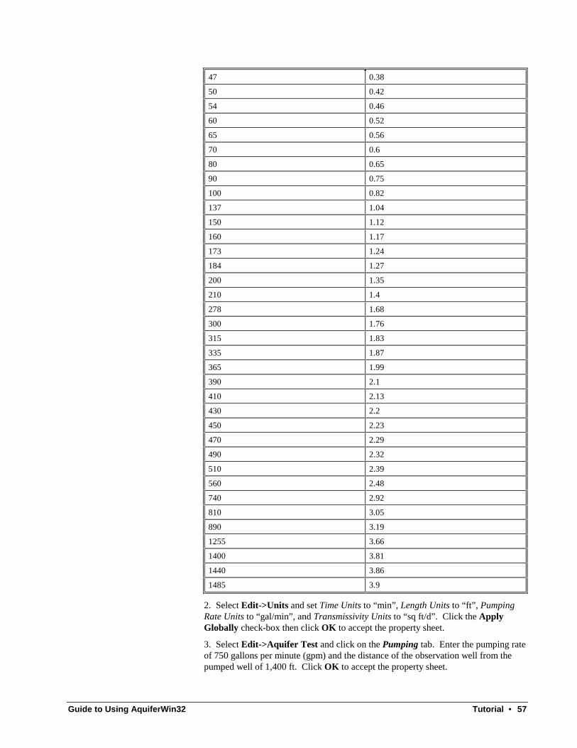
1. Click the button on the Standard toolbar and enter the time and drawdowndata for the test. These data are given in an ASCII text file loh33.dat and in thefollowing table. Remember, to import the ASCII file click on the first row in thespreadsheet and select File->Import. You can also right click on the spreadsheetand select Import from the context menu.
Time (min) Drawdown(ft)
6.37 0.01
8.58 0.02
10.23 0.03
11.9 0.04
12.95 0.05
14.42 0.06
15.1 0.07
16.88 0.08
17.92 0.1
21.35 0.12
21.7 0.13
22.7 0.14
23.58 0.15
24.65 0.17
29 0.21
30 0.22
32 0.24
34 0.26
36 0.28
38 0.3
41 0.33
44 0.36
Guide to Using AquiferWin32 Tutorial • 57
47 0.38
50 0.42
54 0.46
60 0.52
65 0.56
70 0.6
80 0.65
90 0.75
100 0.82
137 1.04
150 1.12
160 1.17
173 1.24
184 1.27
200 1.35
210 1.4
278 1.68
300 1.76
315 1.83
335 1.87
365 1.99
390 2.1
410 2.13
430 2.2
450 2.23
470 2.29
490 2.32
510 2.39
560 2.48
740 2.92
810 3.05
890 3.19
1255 3.66
1400 3.81
1440 3.86
1485 3.9
2. Select Edit->Units and set Time Units to “min”, Length Units to “ft”, PumpingRate Units to “gal/min”, and Transmissivity Units to “sq ft/d”. Click the ApplyGlobally check-box then click OK to accept the property sheet.
3. Select Edit->Aquifer Test and click on the Pumping tab. Enter the pumping rateof 750 gallons per minute (gpm) and the distance of the observation well from thepumped well of 1,400 ft. Click OK to accept the property sheet.

58 • Tutorial Guide to Using AquiferWin32
4. Click on the graph window and then select Edit->Solution. The Solution tab isshown first by default. Change the combobox from “Theis, 1935 (Confined)” to“Hantush, 1960 (Leaky Aquifer with Storage)”. Click the Curves tab to see whichvalues of β will be plotted as separate type curves. You may add additional curvesby clicking the Add button.
5. Click the Parameters tab and ensure the all three Hydraulic Parameters are freeto vary. The small check-boxes that are intended to resemble push pins located to theright of Transmisivity, Storage coefficient and Beta should all be unchecked. If theywere checked, as with Radial distance and Pumping rate, the values would be heldconstant during optimizations.
6. Click OK to accept the property sheet.
You are now ready to analyze the data. It is strongly recommended that a manualmatch be performed first. Using the arrow keys on the keyboard, attempt to manuallymatch the data to the third type curve from the left. Essentially, you try to determinewhich type curve best matches your data. Then, set the combo box on the Matchtoolbar to that value, in this case use “2.00”. You could also toggle through the typecurves by using Ctrl-T on the keyboard. Once you have changed the selected typecurve, make final adjustments to the manual match. A manual match will update theinitial guesses for parameter values based on the match point and the selected typecurve so you must move the data after a new type curve has been selected to updateits initial guess.
The default behavior of the application is to calculate an initial guess for T and Susing a straight line method. Although this works well for some analyses, it doesn’twork for this one; therefore, deactivate this default behavior by clicking the Edit->Solution menu, click the Advanced button on the Solution Information propertysheet and click the Calculate Initial Estimates check-box to remove the check. Ifyou do not deactivate the calculation of initial estimates, you will get an errormessage during an optimization stating that the numerical solution has becomeunstable. This means that the Marquardt procedure could not come up with animproved estimate for T and S. One problem with the Marquardt method is that yourinitial guess for T and S must be fairly close to the “right” answer before it will workproperly. You will get another message after the error dialog that asks if you wouldlike to turn off the option to automatically estimate initial guesses for parameters.Selecting Yes on this dialog does the same thing as removing the check from theCalculate Initial Estimates check-box.
Click the button on the Match toolbar to analyze the test results using thenonlinear least-squares technique. The solution should converge to a T value ofabout 2,190 to 2,200 ft2/d, an S value of about 4.6e-05, and a beta value of 1.76.
In order to have the correct type curve on the graph (for a beta value of 1.76), selectEdit->Solution, click on the Curves tab, select “2.00” in the Curve Information listbox, click the Edit button, and change the value to “1.76”. Click the OK button onthe dialog and the OK button on the property sheet. The type curves will thenrecalculate. Select the 1.76 type curve and click the calculator button. The valuesobtained by Lohman were 2,170 ft2/d and 3.0e-05 for T and S, respectively. Anexample legend can be copied from han60.aqw and pasted into both the Match Dataand Predicted tab views. Your screen should look similar to the one shown below.

Guide to Using AquiferWin32 Tutorial • 59
If you are familiar with other aquifer test software such as AQTESOLV, you will seethat AquiferWin32 has a slightly different philosophy or focus. Whereas most otheraquifer test analysis packages rely heavily on the automatic matching procedures,AquiferWin32 is designed to be more like the visual or manual matching techniquesadvocated by most hydrogeology text books (See Fetter, 1994 for example) and byASTM. AQTESOLV, for example, cannot display a family of type curves (only 1curve and 2 sensitivity curves can be displayed). An alternative view of the matchresults is presented in the Predicted view tab. Click on this tab and also click on theView->Clip Data menu to clip the predicted curve to the graph window. Theresultant graph is the same type of graph presented in AQTESOLV displaying theobserved drawdown versus time data and predicted drawdown versus time curve.This graph can be annotated and modified as required and an example is shownbelow.

60 • Tutorial Guide to Using AquiferWin32

Guide to Using AquiferWin32 Tutorial • 61
Using Multiple Observation Wells
What you will learn:
• analyzing an aquifer test with multiple observation wells
• advanced discussion of unit conversions
• more about adding legends
• optimizing the solution for all wells and for individual wells
• more about using AquiferWin32 as an OLE server
The remaining tutorial examples cover advanced topics in AquiferWin32. Theseexamples are designed to show you how to perform unit conversions, annotate plots,and work with complex data sets.
This section outlines how to analyze a multiple well pump test. The particular dataare taken from Lohman, (1979; page 19). The first step is to create a new
AquiferWin32 Analysis document by clicking on the button on the Standardtoolbar. Once the document is created, the first step is to set the units to be used inthe analysis. The Edit->Units menu displays the Unit Information property sheetwith two tabs. The first tab, Summary, contains the four basic parameters and theirrespective units. The values represent either the program defaults or the valuespreviously saved as default. Under normal circumstances, you would set thesummary units to most closely approximate the units of the data collected. In thisinstance, we will intentionally deviate from the norm in order to demonstrate unitchanges activated from other parts of the program. Set Time Units, Length Units,Pumping Rate Units and Transmissivity Units to “sec”, “ft”, “gal/min” and “sq ft/d”.Click the Save As Default check-box and the Apply Globally check-box. There isno need to click the Convert Data check-box because no data exist yet. (NOTE:Whenever a new parameter or well is created in AquiferWin32, the default valuessaved in this way are used to set the initial units.)
Before exiting the property sheet, click on the Units tab. This tab allows specificparameters to be assigned units. AquiferWin32 allows the ultimate flexibility when itcomes to setting units; however, it is imperative that one understands the paradigm.Every parameter contained in AquiferWin32 has units that can be expressed in terms ofthree generic "units"; these are length (L), time (T) and volume (V) with the possiblevalues organized into three sets of radio buttons. When a parameter is selected in theParameter combobox, the appropriate radio button sets are activated. Simply selectthe desired unit from each radio button set. One of the most complicated parameters,Transmissivity, can be expressed in dimensionless units as V/T/L. If you selectgallons, days and feet for V, T and L the resulting units would be gallons per day perfoot (gal/d/ft). If you select cubic feet, days and feet, the resulting units would besquare feet per day (sq ft/d). (NOTE: If changes are made to both tabs of thisproperty sheet, the values on the Summary tab take priority.) Accept theproperty sheet by clicking the OK button.
Since we are setting up a multiple well scenario, click on the Site Map view tab toactivate it. Now we should set up the map via the Options->Map->Parametersmenu. Click on the Window tab and set both Height and Width to “1000”. If we had

62 • Tutorial Guide to Using AquiferWin32
a basemap of the site, we would click on the File tab and enter a map file name whichwould automatically set the map window dimensions based on the map beingimported. (NOTE: Unlike other ESI software, the map is stored with thedocument so that it is self-contained.) Accept the property sheet and add the wells
by using the Add->Well menu or clicking the button on the Analytic toolbar. Ineither case, the cursor will change to perform a drag insert. Move the cursor to thedesired location on the map and click the left mouse button. For our purposes, putthe cursor anywhere and edit the Well Information property sheet as below.
Although it is a good idea to fully define the pertinent construction parameters, it isnot required for this example. The reason is that the Theis analysis (which we intendto use) does not use any of the well construction parameters. Click on the Display taband click on the Display check-box so that the well name, PW, is displayed and clickon the OK button. In similar fashion, add three more wells using the default wellconstruction information:
Name X Y
N-1 100 300
N-2 500 100
N-3 900 100
Now that the "Site" has been defined, the next step is to define the "Aquifer Test".Click on the Edit->Aquifer Test menu. The first tab of the Aquifer Test Informationproperty sheet contains user-fields. These user-fields can be used to annotate anyGraph or Map View and are also included in the hard copy report. Click on thePumping tab and select “PW” in the Pumping Well combobox. Now we must definethe pumping schedule. Click the left mouse button in the Pumping Rates spreadsheet

Guide to Using AquiferWin32 Tutorial • 63
or Tab into it from the Pumping Well combobox. Hit the Ins key or right click themouse within the spreadsheet and select Insert from the context menu. We nowwant to set the pumping rate to 96,000 ft3/d but the units on the column are gallonsper minute (gpm). Right click the mouse within the spreadsheet and select ColumnConversion to display the Unit Information property sheet as below.
Select “Pumping Rate” in the Column combobox and set the Time units to “days” andthe Volume units to “cubic feet”. Click on the Apply Units and Apply Globallycheck-boxes and click on the OK button. The column title will change to reflect thenew units.
To enter the data, click the mouse in spreadsheet row 1 and column 2 and enter“96000”. At this point, if you were to hit the Tab key or the Enter key a new datarow would be added and you could continue entering the pumping schedule. Hit theEsc key once to clear the field. Now lets assume you really want your pumping ratesdisplayed in gpm. Right click the mouse to bring up the context menu and activatethe Column Conversion menu. With “Pumping Rates” selected in the Columncombobox, set the Volume units to “gallons” and the Time units to “minutes”.Activate Apply Units, Apply Globally and Convert Data then click on the OKbutton. The pumping rate is now displayed as 498.667 gal/min.
The next step is to define the wells monitored during the test. Click the Wells tab andmove wells N-1, N-2 and N-3 from the Available Wells list to the Monitored Wellslist by clicking the Add button three times. (NOTE: This and other Add/Removelist box pairs are Drag and Drop enabled so you can drag items from one listbox to the other.)
To enter the drawdown data for the monitoring wells, click on the Well Data tab.This spreadsheet has tabs along the bottom for the Match Data and each of themonitored wells. Click on the N-1 tab to begin entering the data. By now you

64 • Tutorial Guide to Using AquiferWin32
probably have experience entering data into the spreadsheet using the keyboard so wewill import the data from an ASCII file. Click the right mouse button within thespreadsheet to activate the context menu and select Import. Import the file n-1.datwhich should be contained in the AquiferWin32 directory. Repeat the procedure for theother three monitored wells using n-2.dat for well N-2 and n-3.dat for well N-3.Since this tutorial attempts to represent real world, we must now correct a mistake.The time data contained in the ASCII files are represented in minutes and the units onthe Time columns in the respective spreadsheets is seconds. Activate the contextmenu (right click the mouse) and select Column Conversion. Set the Columncombobox to “Time” and click on the “minutes” radio button. Click on the ApplyUnits and Apply Globally check-boxes and then click the OK button to perform theunit change. The Apply Globally check-box made the unit change to all time datathroughout the data file saving us some time. Obviously, global unit changes withoutdata conversion must be done with care.
After we accept the Aquifer Test Information property sheet by clicking the OKbutton, we are ready for the next step. You will note that the Match Dataspreadsheet to the left of the map has only changed in that the units on the Timecolumn are now minutes due to our global time unit change. We must now define the"Analysis" by using the Edit->Analysis menu. The Analysis tab contains additionaluser fields and determines how the pumping rate is calculated from the pumpingschedule. In this case, the default, Calculate Time Average Pumping, is acceptable.Click on the Match Data tab as shown below.

Guide to Using AquiferWin32 Tutorial • 65
There are various ways to analyze this problem so we will begin with the mosttraditional which is to combine all the wells together adjusted by radial distance. Toaccomplish this, click on the Include Well In Match Data radio button and the AdjustData for Radial Distance check-box. Change the selection in the Well Designatorcombobox to “N-2” and repeat the previous settings. Also, change the Symbol Styleto something other than the default. Repeat the procedure for well N-3 and click theOK button. Since we have made changes to the symbol styles, the following dialogwill be displayed to confirm that we want to reset all symbols. Click the Yes button.
The spreadsheet has now been populated with the resulting data to be analyzed. Atthis point the columns of the spreadsheet may need to be expanded to better see thecolumn titles and data. The easiest way is to click within the spreadsheet and selectthe View->Optimize menu which will make the columns just wide enough to displaytheir contents. Click on the Match Data tab to display the Type Curve Graph. Sincewe have made some unit changes without converting the data, it is good practice toclick the Calc->Reset Data Offset menu to reinitialize the data offsets. Notice that

66 • Tutorial Guide to Using AquiferWin32
the data is nowhere to be seen. This is because the Adjusted Time coordinates aremuch lower than the minimum for the graph. You can either repeatedly hit the rightarrow key until they come into view or optimize the solution via the Calc->Optimizemenu. In this example, optimizing the solution gives a Transmissivity value of13376.4 ft2/d and a Storage coefficient value of .000201527.
Another way to analyze the same data is to include each well individually andoptimize them as a group. Choose the Edit->Analysis menu and click on the MatchData tab. For each monitoring well click on the Include Well Individually radiobutton and click on the Adjust Data for Radial Distance to stop dividing the timedata by radial distance squared. Click on the OK button and the window would looklike the one below.
Now that there are multiple data sets being analyzed individually, things are morecomplicated; however, this flexibility allows more detailed analysis of the data. Thegroup optimization procedure allows total control over which parameters areoptimized across data sets. Before we delve into the intricacies of this procedure it isimportant to understand how to work with multiple data sets. The first thing tounderstand is that each well has its own set of analysis parameters that can bemanipulated individually. To demonstrate, manually match the currently selecteddata set, N-1, to the type curve using the arrow keys. Fine tune the match by holdingdown the shift key while using the arrow keys. To see how close your visual match isto the "optimized" match, activate the Calc->Optimize menu. Toggle between datasets using the Edit->Toggle Data Set menu or the accelerator key Ctrl-D. Noticethat the view tab changes to "Match Data - N-2" to indicate the active well. Also,note that the data values in the spreadsheet change to reflect the active well. Repeatthe manual match and optimize match for this data set and for the N-3 data set. Asyou toggle between data sets the status bar reflects the differing values calculated forTransmissivity and Storage Coefficient. The same results could be achieved bysimply using the Calc->Optimize Group menu which will optimize all data setsindividually because we have not set any parameters to be optimized as a group.
Using this procedure, you can determine the variability of the calculated parameters(Transmissivity and Storage Coefficient) to data from each well. To simulate the

Guide to Using AquiferWin32 Tutorial • 67
previous results when all data were adjusted by radial distance and treated as onedata set, use the Edit->Group Optimize Parameters menu. The Group OptimizeParameters property sheet is an Add/Remove list box pair in which the AvailableParameters list box contains all analysis parameters that are free to vary in each dataset. Click the Add button twice to move both “Transmissivity” and “StorageCoefficient” to the Optimized Parameters list box and click the OK button. Now,clicking the Calc->Optimize Group menu will optimize all three data sets such thatthe best value of Transmissivity and Storage Coefficient are determined. Click theCalc->Optimize Group menu and toggle through the data sets. Notice that the valueof Transmissivity and Storage Coefficient displayed in the status bar are all the sameand, not coincidentally, equal the values calculated using the more traditionalanalysis we performed first.
The final step in any analysis is to prepare a graph for the report. The first thing todo is add a legend to the graph indicating which symbols represent the well data.Click on the Add->Legend menu and drag a rectangle along the bottom of thewindow. After dragging a rectangle, the Legend Information property sheet will bedisplayed. Set the Spatial Parameters such that X1 equals “1”, Y1 equals “.25”, X2equals “9” and Y2 equals “0”. Click on the Contents tab and click the DisplayBorder check-box to deactivate it. Next click the Items tab and click on theAutomatic Maintenance of Graph Data Sets check-box to activate it. Finally,click the OK button to accept the changes. A legend will be displayed containing thesymbol and well name for each data set. In order to edit the label and/or font used,use the Edit->Graph menu to display the Graph Information property sheet. Clickon the Line Styles tab, set the Data Set combobox to “N-1” and enter "Well N-1" inthe Label field. This will override the default label which is the name of the well.Click on the Font button and change the Font to “Times New Roman”, the Font Styleto “Bold”. Click the OK button and then set Color to “Red”. Repeat the procedurefor N-2 and N-3 and click the OK button to accept the changes.
Add a more meaningful title to the graph by right clicking on the graph and selectingGraph from the context menu. On the Graph tab, change the Title field to be"Lohman Theoretical Confined Aquifer Test" and click on the OK button. Nowannotate the graph to display the calculated Transmissivity for all three wells. Usethe Add->Legend menu and drag a rectangle in the lower right area of the graph andset X1 equal to “5”, Y1 equal to “1.5”, X2 equal to “8.5” and Y2 equal to “3.25”.Click on the Contents tab and set the Type combobox to “Solid”. Click on the Itemstab and set the Item Type combobox to “Title Object” and click on the Add button.Set the Title field to "Well N-1" and X, Y to “.25”, “1.25”. Click on the OK button.Repeat the add procedure for wells N-2 and N-3 using X, Y of “.25”, “.75” and X, Yof “.25”, “.25” respectively. Now change the Item Type combobox to “ParameterObject” and click the Add button. The following property sheet should be displayed.

68 • Tutorial Guide to Using AquiferWin32
In the Tree Control List Box, click on the + sign for “Specific Wells” to reveal thedetail. Continue to drill down into “Specific Wells/N-1/AnalysisParameters/Transmissivity” and select “Transmissivity”. Set the X and Y values to“1.1” and “1.25”. Add two more parameters for N-2 and N-3 using X, Y values of“1.1”, “.75” and “1.1”, “.25”. Accept the legend by clicking on the OK button. Theresulting graph is displayed below.

Guide to Using AquiferWin32 Tutorial • 69
Now that the analysis has been performed and the beautification procedure is done,activate the Edit->Group Optimize Parameters menu and remove “Transmissivity”and “Storage Coefficient” from the Optimized Parameters list box by clicking theRemove button twice. Accept the property sheet by clicking the OK button.Activate the Calc->Optimize Group menu and notice that the legend is updated atthe end of each iteration. When the process has completed, you now have a graph inwhich the data from all three monitoring wells have been optimized independentlyand the resulting transmissivity values are displayed.
Now save the analysis document via File->Save As and name the file multwell.aqwand exit the program.
Suppose that you are generating your final report using an OLE Container programsuch as Microsoft Word. Since AquiferWin32 is an OLE Server, you can link thenewly created analysis document directly into the report such that subsequentchanges to the analysis will be automatically updated in your report. To perform thisoperation, start up your OLE Container (e.g. Microsoft Word) and create a newdocument. Click on Insert->Object menu and you should get a property sheetsomething like this:
Notice that there are entries in the Object Type list box for the four AquiferWin32
document types. If you were to select one of them and click the OK button, youwould find yourself in AquiferWin32 editing a new document of the selected type.Such a document would then remain an editable part of the document totally self-contained. Since we want to create an OLE Link click on the Create from File tabwhich will display the following property sheet.

70 • Tutorial Guide to Using AquiferWin32
Click on the Browse button and locate the file multwell.aqw, click the Link to Filecheck-box and close the property sheet using the OK button. When all the windowflashing and disk access stops, the graph from your analysis document will be part ofthe Word document.

Guide to Using AquiferWin32 Tutorial • 71
Double click the mouse on the graph and you will find yourself in AquiferWin32
editing multwell.aqw. Click the mouse within the graph in AquiferWin32 and hit thedown arrow key. Use the menu File->Save to save the change and change windowsto the OLE client software in normal windows fashion. Notice that the graphicwithin the Word document has changed to reflect the change made to the AquiferWin32
analysis.

72 • Tutorial Guide to Using AquiferWin32
Analyzing Recovery Tests
What you will learn:
• analyzing the recovery of an aquifer test
• alternative solution using variable pumping
The first tutorial demonstrated how to analyze a simple aquifer test, one in whichthere is only one observation well. This tutorial shows how to analyze the recoverydata from that same test taken from a real aquifer test reported by Kruseman and deRidder (1990; page 59).
As previously stated, Kruseman and de Ridder call this aquifer test Oude Korendijkfor the area where the test was conducted. The pumping well was screened over theentire aquifer thickness of 7 meters. Piezometers were placed at distances of 0.8, 30,90, and 215 meters. The well was pumped at a constant discharge rate of 0.547m3/min for 14 hours. This tutorial will use time and drawdown data includingrecovery for the 30 meter piezometer.
Entering Data
Start a new aquifer test by clicking the button on the Standard toolbar or selectFile->New. The default graph type is for the Theis confined analysis which we willchange after the data has been entered. The first thing you should do when starting anew analysis is to set the units for the pumping test data. Select Edit->Units to tellAquiferWin32 what units you are using. In this case, select minutes (min) for TimeUnits, meters (m) for Length Units, meters cubed per minute (cu m/min) for PumpingRate Units, and square meters per minute (sq m/min) for Transmissivity Units. Clickthe Apply Globally check-box at the bottom of the property sheet to set these unitsfor the entire analysis including all data types and accept the property sheet byclicking the OK button.
Import the drawdown versus time data including recovery from the file fulltest.dat.To import the data from a text file, click on the first line in the spreadsheet tohighlight that row. Select File->Import and find the file. AquiferWin32 will notifyyou that 51 lines were imported. If necessary, delete the default 1,1 data point.
It is important to note that the data for a recovery test is the same as for a pumpingtest. Time is relative to the start of pumping and drawdown is relative to the originalstatic water level before pumping began. You do not have to delete the data from thepumping test because the recovery analysis will automatically ignore it.
Now that we have the time and drawdown data, we will enter the remaining test data.Select Edit->Aquifer Test to enter the pumping rate and distance to observationwell. Click on the Pumping tab on this property sheet and enter the followinginformation:
Pumping Well Name P1
Pumping rate 0.547 m3/min.
Pumping well screen length 7 m
Monitoring Well Name H30

Guide to Using AquiferWin32 Tutorial • 73
Radial Distance 30 m
Screen length 7 m
The property sheet should resemble the one below. Click OK when you are done.
Traditional AnalysisAt this point, click the Edit->Solution menu to activate the Solution Informationproperty sheet. Select “Theis, 1946 (Recovery)” in the solution combobox. Clickthe Parameters tab and enter “830” into the Time Recovery Starts edit field.(NOTE: Forgetting to enter the Time Recovery Starts correctly is the mostcommon mistake made using this analysis; it is used to properly convert thedata for the analysis.) Accept the property sheet by clicking the OK button. Theresulting graph is shown below. The data points prior to recovery are not displayedand a linear regression has been performed to calculate a transmissivity of .31m2/min.

74 • Tutorial Guide to Using AquiferWin32
In a recovery test, as with other tests, the late data is usually assumed to be morerepresentative. In this case, the late data is on the left of the graph because it hasbeen scaled during the analysis. Click the Edit->Aquifer Test menu and click on theWell Data tab. Change the weight on lines 35 through 39 to 100 which will removethem from consideration for the purposes of linear regression. Also, change thesymbol to a triangle for the same data points to visually indicate which points arebeing ignored. Accept the property sheet by clicking the OK button. Now click theCalc->Optimize menu to recalculate an answer.

Guide to Using AquiferWin32 Tutorial • 75
Variable Pumping AnalysisThe linear regression Theis recovery analysis is the traditional method for analyzingrecovery data; however, AquiferWin32 offers another alternative. Since AquiferWin32
supports variable pumping rates, we can analyze the pumping and recovery datasimultaneously. To set up for this analysis we must add wells to the site map to setup for a multiple well analysis. Click the Site Map tab on the view to activate themap. Click the Add->Well menu and left click the mouse somewhere on the map.The Well Information property sheet will be displayed. Enter the values as below.
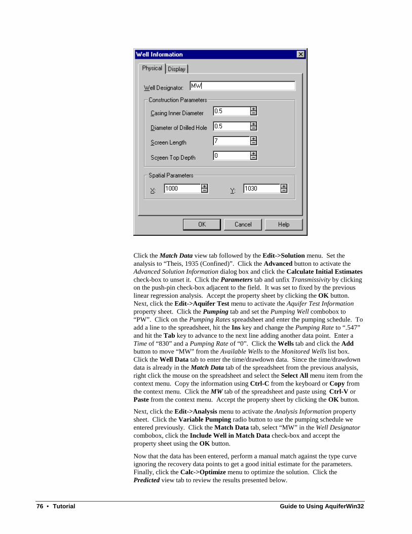
Repeat the procedure to add the monitoring well and enter the values as below.
76 • Tutorial Guide to Using AquiferWin32
Click the Match Data view tab followed by the Edit->Solution menu. Set theanalysis to “Theis, 1935 (Confined)”. Click the Advanced button to activate theAdvanced Solution Information dialog box and click the Calculate Initial Estimatescheck-box to unset it. Click the Parameters tab and unfix Transmissivity by clickingon the push-pin check-box adjacent to the field. It was set to fixed by the previouslinear regression analysis. Accept the property sheet by clicking the OK button.Next, click the Edit->Aquifer Test menu to activate the Aquifer Test Informationproperty sheet. Click the Pumping tab and set the Pumping Well combobox to“PW”. Click on the Pumping Rates spreadsheet and enter the pumping schedule. Toadd a line to the spreadsheet, hit the Ins key and change the Pumping Rate to “.547”and hit the Tab key to advance to the next line adding another data point. Enter aTime of “830” and a Pumping Rate of “0”. Click the Wells tab and click the Addbutton to move “MW” from the Available Wells to the Monitored Wells list box.Click the Well Data tab to enter the time/drawdown data. Since the time/drawdowndata is already in the Match Data tab of the spreadsheet from the previous analysis,right click the mouse on the spreadsheet and select the Select All menu item from thecontext menu. Copy the information using Ctrl-C from the keyboard or Copy fromthe context menu. Click the MW tab of the spreadsheet and paste using Ctrl-V orPaste from the context menu. Accept the property sheet by clicking the OK button.
Next, click the Edit->Analysis menu to activate the Analysis Information propertysheet. Click the Variable Pumping radio button to use the pumping schedule weentered previously. Click the Match Data tab, select “MW” in the Well Designatorcombobox, click the Include Well in Match Data check-box and accept theproperty sheet using the OK button.
Now that the data has been entered, perform a manual match against the type curveignoring the recovery data points to get a good initial estimate for the parameters.Finally, click the Calc->Optimize menu to optimize the solution. Click thePredicted view tab to review the results presented below.

Guide to Using AquiferWin32 Tutorial • 77

78 • Tutorial Guide to Using AquiferWin32
Analyzing Slug Tests
What you will learn:
• analyzing a slug test
• using different slug test analysis techniques
• more about unit conversions
Slug tests seem to be routine in many field investigations because they are simple andcost-effective to perform. If you are looking for a procedure to perform all slug tests,this tutorial may be the answer. The first step is to use the File->New menu to create
a new document since the button on the Standard toolbar defaults to an“AquiferWin32 Analysis” document. Select “AquiferWin32 Slug Test” from the listbox and click the OK button. The default analysis for a slug test is the traditionallinear regression version of Bouwer and Rice.
The next step is to enter the time and displacement data. The particular data set wewill use is taken from Lohman (1979; page 29). The data represent recovery in awell under confined conditions.
To continue our theme of making life a little easier, the data is stored in the filedawson.dat. Before importing the data, however, activate the spreadsheet view byclicking the mouse in the column title part of the spreadsheet. Use the Edit->Unitsmenu and set the values as below.
Accept the property sheet by clicking the OK button. Next, import the data by rightclicking the mouse on the spreadsheet and selecting Import from the context menu.

Guide to Using AquiferWin32 Tutorial • 79
Locate the file dawson.dat and load in the data. Notice that the import has left theinitial data value 1,1. Click the left mouse button on the line number column(leftmost column) and hit the Del key to delete the row. Now, click the mouse in thegraph view and, resisting the temptation to use the Calc->Optimize menu, click onthe Edit->Aquifer Test menu. At this point, skip the user fields and click on theWell tab. It is important to complete the well construction information on this tabbecause the analysis requires it. The field book says that: "the well is cased to 24 mbelow the top of the aquifer with 6 inch casing and drilled as a 15.2 cm open hole toa depth of 122 m and the theoretical initial displacement should be .56 m". Put ameaningful value in the Well Name field like "Well". Now enter the Casing InnerDiameter which is initially set to “.5” meters. If you are unsure of the units, movethe mouse cursor over the Casing Inner Diameter field and wait. The units "m" willbe displayed as a tool tip and the status bar will display "Casing Inner Diameter (m)".
Lets take a moment to learn about units and unit conversions. In this case, we have afield that wants meters and we have a value in inches. Let us assume that ourcalculator battery died. You now have several options. The obvious first option is todo the conversion manually and enter the value. A second option is to right click onthe Casing Inner Diameter field, select the Units menu, change the units to inches,click the OK button and enter 6 into the field. The system doesn't care what unitsyou use because it internally converts all data before performing calculations. Youcan go wild and use whatever units you want on a parameter by parameter basis.(This is not recommended if you are using Windows 3.x since the tool tip reminderas to unit values doesn't work!) For our purposes here, click the Cancel button tocancel the changes.
Click on the Edit->Aquifer Test menu again and feel free to fill in any user fields onthe Test tab before clicking to the Well tab. After entering something meaningful inthe Well Name field, enter “6” in the Casing Inner Diameter field. Right click on theCasing Inner Diameter field and select Data Conversion from the context menu.Click on inches in the Length radio buttons of the From tab of the embeddedproperty sheet to indicate the units of the previously entered value. Click on the Totab and notice that the units to convert to are not editable and reflect the prevailingunits of the parameter being edited. Now click the Convert button followed by theOK button. The value of 6 inches has been converted to meters and the field hasbeen updated with the converted value.
To complete the data entry, type “.1524”, “98” and “24” in the Diameter of DrilledHole, Screen Length and Screen Top Depth fields. Finally, enter “.56” into theInitial Displacement field and accept the property sheet by clicking the OK button.
The next step is to click on the Edit->Solution menu and update any additionalparameters that are required for the analysis. Since this is a linear regressionsolution, the Convergence Information on the Solution tab is disabled. Click on theWell Parameters tab and note the previously entered well construction parametersare being used and there is one additional parameter. The Gravel Pack Porositydefaults to “.3” which is fine. In fact, unless the water is recovering within the screenor open hole interval, this value is not used by the analysis. It is important to note atthis point the custom check-boxes to the right of the fields. The lower check-boxindicates whether the parameter is "linked" to a value entered at another section ofthe program. In this case, the first four parameters are linked to the values previouslyenter in the Aquifer Test Information property sheet. Should we choose to do so, wecan unlink any or all of the values and enter an override value. This action will notchange the linked value and the linked value can be restored by relinking theparameter. The upper check-box is not used in a linear regression analysis; however,

80 • Tutorial Guide to Using AquiferWin32
it determines if the parameter is free to vary in a curve match scenario. A linkedvalue is always fixed so it has to be unlinked to be estimated by the program.
Click on the Hydraulic Parameters tab and change the Aquifer Thickness to “124”.If we wanted to simulate recovery within the well screen, the Maximum Water Depthshould be set so the program can determine if such a condition exists. Now click onthe Well Results tab and notice an additional parameter is present that was notpresent on the Well Parameters tab. The Effective Casing Inner Diameter is acalculated value used by the analysis that differs from the Casing Inner Diameteronly if recovery is occurring within the screened interval. Click on the HydraulicResults tab and notice three additional calculated parameters which are specific tothis analysis. An attempt has been made to provide you with all the values you wouldneed should you want to do the calculations on paper. Accept the property sheet byclicking on the OK button.
Now the time has come to calculate the optimized solution. For this analysis, theoptimized solution is achieved via linear regression. Click in the graph view and
click the button on the Match toolbar or use the Calc->Optimize menu. Noticethat a linear regression has been performed on the data and the Bouwer and Ricesolution has been calculated. What a minute, this is supposed to be a confinedanalysis and the value for initial displacement should be .56 not the .453982calculated by linear regression. Lets ignore for the moment that we know thesolution is confined.
There are two primary ways to determine the initial displacement, H0, and the slopeof the line. The first way is to manually set it. Move the mouse cursor over thelinear regression line near the center of the graph. The cursor will change to theNSEW cursor (the one with arrows pointing up, down, left and right). Double clickthe left mouse button and the Regression Line Information property sheet isdisplayed.
Actually, this property sheet is the best way to set H0 so change Intercept to the valuewe know to be cast in stone, “.56” meters. Now if you are a veteran slug tester or ifyou read Bouwer and Rice, you know that the slope of the line and the wellconstruction parameters are the only parameters that are involved in the calculation.How then do we proceed? Accept the property sheet by clicking the OK button.You now have a "best fit line" that doesn't hit any of the data points. (There areactually three lines on your screen; the outermost lines are actually part of the

Guide to Using AquiferWin32 Tutorial • 81
rectangle that surrounds the line and indicates that the line has been selected. If youclick the left mouse button outside of this rectangle the selection will disappear.)Now, move the mouse cursor over the rightmost section of the line. The cursor willchange to an EW (arrow left and arrow right) cursor indicating that you can move it.Click the left mouse button, hold it down and drag the end of the line around untilyou are satisfied that you have generated an acceptable match to the data. Notice thatas you drag the line around, the calculated value of hydraulic conductivity, K,changes too. If you were to move the entire line, the calculated value of K would notchange because only the slope matters. Incidentally, the same procedure works forthe left portion of the regression line so you never have to use the Regression LineInformation property sheet as you did above; simply move the left portion of the lineto reset the H0 (intercept) value. However you slice it, you have full control on thesolution just as you would if you were doing it on paper.
The second approach is for those people who are drawn to the optimize button. Howcan we change the "optimized" solution? Right click the mouse on the spreadsheetand select the Columns menu from the context menu. An Add/Remove list box pairis displayed showing that there are two additional columns available to you. Moveboth the weight and symbol columns from the Available Columns to the DisplayedColumns by clicking the Append button twice and click the OK button. Where arethey? Use the View->Optimize menu to optimize the spreadsheet so that all columnsare visible and only as wide as they need to be. (NOTE: You can also access thesedata from the Well Data tab on the Aquifer Test Information property sheet).Change the weight on data rows 5 through 21 to a number of 100 or greater. For alllinear regression analyses, a weight of 100 or greater removes the point fromconsideration during the linear regression calculation. You can also change thesymbol displayed for these data by double clicking the mouse on the current symboland changing it. This would give a visual indication of which data were ignored. Inthis case, H0 is calculated to be .516 and not the theoretical value of .56; however, itis not always possible to know the theoretical H0 and the data may be the onlyindicator as to its value. The important point is that you have lots of ways to performthe analysis.
Since manually changing the weights and symbols can be time consuming, you coulddrag select lines 5 through 21 and click the Edit->Selection menu. On the SelectionEdit Options property sheet, click on the Weight tab. Click the Set Value radiobutton and enter 100 into the adjacent edit field. Now click on the Symbol tab, clickthe Set Value radio button, change the Symbol combobox to a triangle and accept theproperty sheet. This option is easier for bulk changes to the spreadsheet.
Now lets assume you are convinced that the Bouwer and Rice solution is appropriate.How would you know? AquiferWin32 takes a step toward answering that question witha second Bouwer and Rice solution base on a curve match. Change the weights allback to 1 and all the symbols back to the same style if you changed them. You mayalso want to slide the splitter bar over to hide the Weight and Symbol columns. Youcould also remove the columns in an analogous manner to the one used to add themearlier.
Click on the Edit->Solution menu and select “Black, 1978 (Unconfined Aquifer)” inthe Analysis combobox. If you look through the property sheet, you will notice thatnothing has changed from Bouwer and Rice. Click the Hydraulic Parameters taband click on the push pin check-box next to the Hydraulic Conductivity field. Theprevious linear regression analysis initialized the value to fixed. Accept the propertysheet by clicking OK and attempt to match the data to the curve using the arrowkeys. Use the Edit->Aquifer Test menu to activate the Aquifer Test Informationproperty sheet and click on the Well tab. Change the Initial Displacement to “.56”and try again. Notice that the data is automatically rescaled to the new value and

82 • Tutorial Guide to Using AquiferWin32
doesn’t match any better. Obviously, this data doesn’t represent an unconfinedaquifer response as shown below.
Another step to try is to click the Edit->Solution menu and go to the HydraulicParameters tab. Unlink and unfix the Initial Displacement value by clicking both of
the check-boxes to the right of the field so it looks like this . Accept theproperty sheet by clicking the OK button. Now click Calc->Optimize button andlook at the results. This process will optimize both T and H0 but doesn’t result in agood match. The validity of this step is determined by how confident you are withthe value of H0.
Since the unconfined solution did not give an acceptable match and because we knowthe response is confined, we will move on to the confined solution. Click on theEdit->Solution menu and select “Cooper, Bredehoeft & Papadopulos, 1967(Confined Aquifer)” for a confined slug test analysis. Click on the HydraulicParameters tab and relink the Initial Displacement by clicking on the lower of thetwo check-boxes to the right of the field. Now click on the OK button. The systemwill calculate the 10 standard type curves for this analysis. Use the arrow keys tomatch the data to the third curve from the left. Hit the Ctrl-T key twice to select thatcurve (the currently selected type curve changes color), fine tune your match andlook to the status bar for the answer.
To get an optimized solution, go ahead and select the Calc->Optimize menu. Noticethat now the optimized solution has matched to a curve that is not displayed. Clickon the Edit->Solution menu and click on the Hydraulic Parameters tab and click onthe little push pin check-box to the right of the Alpha field. This will "fix" theparameter and remove it from optimization. Set the value to .001 and click on theApply button to optimize the match. This would essentially optimize the manualmatch we did earlier. Click on the little right arrow at the upper right of the propertysheet to advance the tabs and click on the Statistics tab to quantify the "accuracy" ofthe curve match. The residual standard deviation is .004379. Now click on theExceptions tab, select “Initial Displacement” in the Parameter combobox and clickon the Linked Value check-box followed by the Fixed Value check-box; this tabprovides an alternative way to link/unlink and fix/unfix parameters and also shows

Guide to Using AquiferWin32 Tutorial • 83
you where range information can be set for each parameter. It is sometimesnecessary to enforce minimum and maximum parameter values to achieve anoptimized match. In this case, they are not necessary so click on the Apply button.Notice that the calculated value for Initial Displacement has changed to .547477 anda look at the Statistics tab reveals a residual standard deviation of .003467.
How do I optimize the solution for Alpha and get the curve on the graph? Go back tothe Hydraulic Parameters tab and click on the push pin check-box next to Alpha andclick on the Apply button. Now click on the Hydraulic Results tab to see thecalculated values or look in the status bar. Go to the Curves tab and decide whatcurves you want on the graph. Remove all but one of the values from the CurveInformation list box by selecting them and clicking the Delete button. Select the oneremaining value and click on the Edit button. Change the value to “.000136”,change the Label Format to “EXPONENTIAL” and change the Precision to “6” andclick the OK button on the property sheet. Click the OK button on property sheetand there is your optimized answer. If you are not concerned with having the exacttype curve represented on the graph you can skip this last step and use the Predictedview tab which displays the observed displacement data with the predicteddisplacement curve through the data.
The final step in any analysis is to prepare a graph for the report. The first thing todo is add a legend to the graph indicating what the symbols represent. Click on theAdd->Legend menu and drag a rectangle along the bottom of the window. Afterdragging a rectangle, the Legend Information property sheet will be displayed. Setthe Spatial Parameters such that X1 equals “1”, Y1 equals “.25”, X2 equals “9” andY2 equals “0”. Click on the Contents tab and click the Display Border check-box todeactivate it. Next click the Items tab and click on the Automatic Maintenance ofGraph Data Sets check-box to activate it. Finally, click the OK button to accept thechanges. A legend will be displayed containing the symbol and well name for eachdata set. In order to edit the label and/or font used, use the Edit->Graph menu todisplay the Graph Information property sheet. Click on the Line Styles tab, set theData Set combobox to “Time/Drawdown” and enter "Well Response" in the Labelfield. This will override the default label which is “Time/Drawdown”. Click on theFont button and change the Font to “Times New Roman” and the Font Style to“Bold”. Next, change the Color to “Red”.
Add a more meaningful title to the graph by right clicking on the graph and selectingGraph from the context menu. On the Graph tab, change the Title field to be"Dawsonville Slug Test" and click on the OK button. Now lets annotate the graph todisplay the calculated Transmissivity, Alpha and Storage Coefficient. Use the Add->Legend menu and drag a rectangle in the lower left area of the graph and set X1equal to “1.2”, Y1 equal to “1.2”, X2 equal to “4.25” and Y2 equal to “3.0”. Click onthe Contents tab and set the Type combobox to “Solid”. Click on the Items tab andset the Item Type combobox to “Parameter Object” and click on the Add button. Thefollowing property sheet should be displayed.

84 • Tutorial Guide to Using AquiferWin32
In the Tree Control List Box, click on the + sign for “Current Well” to reveal thedetail. Continue to drill down into “Current Well/AnalysisParameters/Transmissivity” and select “Transmissivity”. Set the X and Y values to“0.25” and “1.25”. Add two more parameters, “Alpha” and “Storage Coefficient”using X, Y values of “.25”, “.75” and “.25”, “.25” and click on the Units check-box toturn off display of the units. Accept the legend by clicking on the OK button. Theresulting graph is displayed below.

Guide to Using AquiferWin32 Tutorial • 85
Simulating Aquifer Tests
What you will learn:
• simulating an aquifer test
• plotting simulated drawdown contours
• plotting simulated hydrographs at observation wells
The Professional version of AquiferWin32 can also be used to simulate pump tests. Ifyou have an idea of the type of response and hydraulic properties of an aquifer, youcan estimate the aquifer response to a given pumping rate. The response can bedepicted as contour maps at given times and drawdown versus time graphs at anynumber of monitoring wells.
First, use the File->New menu and create an “AquiferWin32 Simulation” document.The only visible object on the Test Simulator view is an arrow. This arrow is thereference head arrow used to define the uniform flow field from which to subtract thedrawdown predicted by the analysis. To edit the parameters click the Edit->Reference Head menu. We are not going to change any of the values because weare interested in a contour map of drawdown. Given this fact, click the View->Reference Head menu to hide the reference head arrow.
As with other tutorials, use the Edit->Units menu to set up the units to be used forthe simulation. Edit the values as below.
Instead of using the Add->Well menu to add wells to the map, click on the Edit->Map Items menu to display the Map Item Information property sheet. Set the ItemType to “Well Object” and click the Add button. The Well Information property
86 • Tutorial Guide to Using AquiferWin32
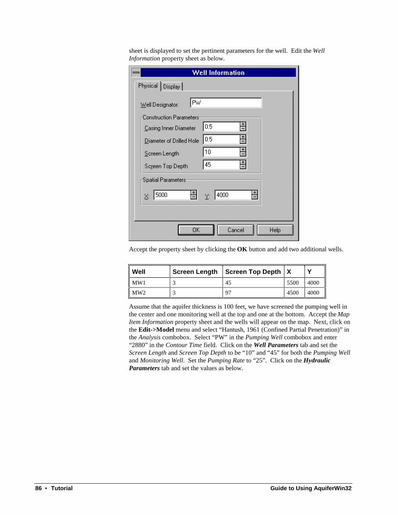
sheet is displayed to set the pertinent parameters for the well. Edit the WellInformation property sheet as below.
Accept the property sheet by clicking the OK button and add two additional wells.
Well Screen Length Screen Top Depth X Y
MW1 3 45 5500 4000
MW2 3 97 4500 4000
Assume that the aquifer thickness is 100 feet, we have screened the pumping well inthe center and one monitoring well at the top and one at the bottom. Accept the MapItem Information property sheet and the wells will appear on the map. Next, click onthe Edit->Model menu and select “Hantush, 1961 (Confined Partial Penetration)” inthe Analysis combobox. Select “PW” in the Pumping Well combobox and enter“2880” in the Contour Time field. Click on the Well Parameters tab and set theScreen Length and Screen Top Depth to be “10” and “45” for both the Pumping Welland Monitoring Well. Set the Pumping Rate to “25”. Click on the HydraulicParameters tab and set the values as below.

Guide to Using AquiferWin32 Tutorial • 87
Click on the OK button to accept the values and click the Calc->Recalculate menuto calculate the simulation. The resulting contour map represents a projection of thedrawdown expected in monitoring wells screened between 45 and 55 feet in responseto a pumping well similarly screened pumping at 15 gpm for 2 days.
Next we will adjust the contour parameters. Click on the Options->Contour->Parameters, change the Minimum Level to “-8.5” and the Interval to “.25”. Clickon the Labels tab and change Distance between to “2000”. Click on the Font buttonand change the point size to “14” and change the Font Style to “Bold”. Click on theOK button and click on the Yes button in response to the subsequent message box.Click the View->Full->Screen menu to adjust the map scale. The resulting windowis shown below.

88 • Tutorial Guide to Using AquiferWin32
To generate drawdown versus time data for the two monitoring wells previouslyadded to the map, click on the Edit->Simulation menu and click on the Add buttontwice to move “MW1” and “MW2” from the Available Wells list box to theMonitored Wells list box. Click on the Well Data tab and notice that the spreadsheethas three tabs along the bottom. One tab for each monitored well and the SimulationTimes tab. The values contained in the Simulation Times tab are used for allmonitored wells. Click on the OK button to accept the property sheet and click theCalc->Recalculate menu to calculate the solution. To view the graphic results, clickthe View->Well Data menu to add two additional tabs to the view. Click on both ofthe new tabs to view the results. Click on the View->Clip Data menu to clip all datapoints not contained within the limits of the graph. The difference between the twographs is caused by the effects of partial penetration.
Now we want to adjust the graph to display the same axis scales. Although we couldchange them individually, an easier way is to click the Edit->Default Well Graphmenu. Click the X-Axis tab and enter “.01” for the Minimum X edit field and click onthe Automatic Minimum check-box to unset it. Click the Y-Axis tab and click onthe Automatic Minimum check-box to unset it. Click the OK button to accept theproperty sheet. In order to activate the defaults, click the Edit->Simulation menuand go to the Wells tab. Click the Remove button twice to remove the wells. Nowadd them back to the Monitored Wells list using the Add button. When we removedthem the graph parameters were removed. Adding them, initializes graph parametersusing the Default Well Graph parameters. Click the OK button to accept thechanges. Click the Calc->Recalculate menu and the graphs are as presented below.

Guide to Using AquiferWin32 Tutorial • 89

90 • Tutorial Guide to Using AquiferWin32
Water Table AquifersWhat you will learn:
• Using Neuman’s Water Table Analysis Method
This section outlines how to analyze an unconfined aquifer pump test. The particulardata are taken from Lohman (1979; page 38, Table 14). The first step is to create a
new analysis document by clicking on the button on the Standard toolbar. Thistoolbar button creates a new “AquiferWin32 Analysis” document whereas the File->New menu presents the four potential document types.
Once the document is created, the first step is to set the units to be used in thesimulation. The Edit->Units menu displays a property sheet with two tabs. The firsttab, Summary, contains the four basic parameters and their respective units. Thevalues represent either the program defaults or the values previously saved as default.Under normal circumstances, you would set the summary units to most closelyapproximate the units of the data collected. Set Time Units, Length Units, PumpingRate Units and Transmissivity Units to “min”, “ft”, “gal/min” and “sq ft/min”. Clickthe Save As Default check-box and the Apply Globally check-box. There is noneed to click the Convert Data check-box because no data exist yet. Accept theproperty sheet by clicking the OK button.
Click on the Edit->Aquifer Test menu. The first tab of the Aquifer Test Informationproperty sheet contains user-fields. These user-fields can be used to annotate anygraph or map view and are also included in the hard copy report. Click on thePumping tab and enter “PW” as the Well Name in the Pumping Well section andenter “1080” into the Pumping rate field. Enter “MW” as the Well Name in theMonitoring Well section and enter “73” in the Radial distance field. The remainderof the well construction information is not required since this analysis will notconsider partial penetration.
To enter the well response data for the monitoring well, click on the Well Data tab.This spreadsheet has one tab along the bottom for the match data. Click on the rownumber column of the first data row to select it and hit the Del key to delete the datarow. By now you probably have experience entering data into the spreadsheet usingthe keyboard so we will import the data from an ASCII file. Click the right mousebutton within the spreadsheet to activate the context menu and select Import toimport the data from the file unconf.dat.
After we accept the Aquifer Test Information property sheet by clicking the OKbutton, we are ready to select the analysis to use. Click the left mouse button in thegraph view to activate its menu. Select the Calc->Reset Data Offset menu which isgood practice when changing units without converting the data. Click the Edit->Solution menu, click on the Analysis combobox and select “Neuman, 1972(Unconfined Aquifer)”. Click on the Parameters tab and notice the Radial distanceand Pumping rate have been updated based on our previous entries in the AquiferTest Information property sheet. Set the Specific Yield to be two orders of magnitudehigher than the value of Storage coefficient and click the “Push Pin” check-box on
the control adjacent to the Specific Yield field so it looks like this . Thevalues entered on this tab represent our initial guesses for the analysis and all “fixed”

Guide to Using AquiferWin32 Tutorial • 91
values are transferred to the calculated values as well. In this case, we want totransfer the adjustment of Specific Yield to the calculated values to affect the typecurves being generated. Strictly speaking, this step is not necessary but will generatea better set of type curves. (NOTE: The ratio of Storage coefficient and SpecificYield dictate the offset between the “Early” and “Late” portions of the typecurves). Click on the Curves tab and set the contents of the Curve Information listbox to “0.001”, “0.01”, “0.05”, “0.10” and “1.00”. Click on the OK button and thescreen should appear as below.
Click on the Calc menu and make sure there is a check mark next to the MatchEarly Data menu. If it is not, click on the Calc->Match Early Data menu. Movethe data around using the arrow keys to perform a manual match of the early (leftmost) data points to the left side of the type curves. Use Edit->Toggle Type Curveor Ctrl-T to select the appropriate type curve. Look at the status bar and note thevalues for T and S which are representative of matching the early data (the initialconfined response). Although matches are subjective, match to a T of approximately20.3 and an S of approximately .0025 using the .05 type curve. Next, click the Calc->Match Late Data menu to match the late data. Notice that the data moves and thestatus bar T and S change. This is because both the Early and Late Matches are keptindependently as if they were two separate monitoring wells. Repeat the procedurefor the late (right most) data to determine T and S for the late data (the unconfinedresponse). This time, match to a T of approximately 23.6 and an S of approximately0.111 using the .05 type curve. As you toggle between the early and late solutions,you can see the difference in the value of T.
Now that you have made your two matches as prescribed by the analysis you havefinished the traditional solution. To improve the presentation of the results, you canclick Calc->Recalculate Type Curves to calculate a set of type curves consistentwith the new Storage Coefficient and Specific Yield ratio. By recalculating the typecurves, you will have to reset the selected type curve. This step gives you better typecurves than the traditional ones in the literature because they have been calculatedspecifically to your solutions. Use Ctrl-T to toggle the type curve selection back tothe .05 type curve.

92 • Tutorial Guide to Using AquiferWin32
If you want to get an optimized solution and eliminate the need for two separatematches, click Edit->Solution, click on the Parameters tab and unfix Specific Yieldas discussed before. Alternatively, you could click on the Exceptions tab, set theParameter combobox to “Specific Yield”, and click the Fixed Value check-box tounset the check. In either case, you are allowing Specific Yield to be optimized.Click the Solution tab and click the Advanced button and click off the CalculateInitial Estimates check-box. The initial estimates calculation is not necessarybecause we performed a manual match. In some cases, this being one, the initialestimates calculation can cause the solution to become unstable. Click the OKbutton to close the property sheet and click the Calc->Optimize menu. To see theresults of the optimization, click on the Edit->Solution menu and go to the Resultstab. If you would like the exact type value of .0468 instead of .05, click on theCurve tab and change Value from .05 to .0468 and set Precision to “3”. Since acurve value was changed, the type curves will automatically be recalculated. Theoptimized view is as below.

Guide to Using AquiferWin32 Tutorial • 93
Step Test Analysis
What you will learn:
• Using the Eden and Hazel method to determine well performance
• Automatic and manual matching procedures
For this particular test, users are guided through the input and analysis of a data settaken from Kruseman and De Ridder (1994), page 204. These data are also used inan example file (clarke4.aqp) which can be used to check the analysis results. Thedata was taken from Clarke L. (1977), The analysis and planning of step-drawdowntests. Q. Jl. Eng. Geol, volume 10.
The first step is to set up a new file in which to input the step test data. Selecting theFile->New menu displays the five types of documents or analysis types, including“AquiferWin32 Flow Model”, “AquiferWin32 Analysis”, “AquiferWin32Simulation”, “AquiferWin32 SlugTest” and “AquiferWin32” StepTest. Select“AquiferWin32 StepTest” and click the OK button. This action will bring up thedefault Eden and Hazel (Part 1) screen.
The next step is the specification of the units to be used in the input and analysis. Itis recommended that these be specified at this stage, although as you know, the unitscan be modified after input. For this example, set Time Units, Length Units,Pumping Rate Units and Transmissivity Units to “min”, “m”, “cu m/d” and “sq m/d”.Click the Save As Default check-box and the Apply Globally check-box. There isno need to click the Convert Data check-box because no data exist yet. Accept theproperty sheet by clicking the OK button.
Once the step test has been selected and the units of input chosen, the data inputprocess can begin. You should be familiar by this stage with the options for inputtingdata and be well versed in all of the methods. Since this is a large data file, it isrecommended that the file clarkedd.dat be imported as an ASCII file using the File->Import menu option. This file contains only the drawdown/time data and whenimported the file should contain 174 lines. It is again important to remove the initialdefault value from the first row of the time/drawdown column. Next enter thepumping rate and time data. This is entered by selecting the Edit->Aquifer Testmenu, clicking the Pumping tab and entering the data on the table as shown below.

94 • Tutorial Guide to Using AquiferWin32
Accept the property sheet by clicking the OK button. Normally, the graph axes willautomatically rescale to match the data; however, if you now look at the graph, thedata may appear to be missing. This is not due to its abduction but to the fact that theaxes will have to be rescaled to allow the display of this data. In this particular casethe maximum on these linear scaled axes should be set such that the maximum valuefor x is 24000 and the maximum value for y is 30. Click in the graph view andactivate the Edit->Graph menu. Click the X-Axis tab and enter “24000” in theMaximum X field and click the Automatic Maximum check-box to unset it. Clickthe Y-Axis tab and enter “30” in the Maximum Y field and click the AutomaticMaximum check-box to unset it. When new data sets are to be analyzed thedrawdown or y-axis can be scaled according to the maximum value of drawdownencountered. In the case of the x-axis it is suggested that the initial scale be set to ahigh value to display the whole data set and that it is scaled down to increaseresolution of the data at an appropriate lower value of H as desired.
At this point it is worth mentioning data weighting. Some of the early data in thedata sets will not be very useful in the analysis. If it is desired that some of this databe excluded from the analysis, go to the Edit->Aquifer Test menu, Well Data tabwhich can be used to change the weighting of some data points. If the weight on apoint is set to 100 or greater, it is then after excluded from the analysis. A change inthe symbol type can be used in conjunction with this function to allow the user todistinguish excluded data on the graph. The resulting graph is shown below.

Guide to Using AquiferWin32 Tutorial • 95
Now that these initial data have been entered the test is ready to run. However it isworth noting that there are a number of extra inputs which are specified in theproperty sheet. The Edit->Site, Edit->Aquifer Test and Edit->Analysis menusactivate property sheets that can be used for the input of details which can be laterdisplayed in the form of title boxes, headers, footers, parameter boxes etc. Thedetails can be entered into the defined boxes or one of the “ User Fields” in the Usertab of each property sheet. User fields are customizable parameter fields which allowinput of a wide range of preferred data or text items. Click on the Edit->Site menuto bring up the Site Information property sheet. If you click on the User tab, you willsee that each field has a default name. This default name can be changed easily byfollowing the following instructions. Right click the mouse on the title for User Field1 to activate the context menu and select the Edit menu. Enter “Date” into the UserField Title field and click OK to accept the dialog. Repeat the procedure to set UserField 2 to “Start Time”. If you activate the context menu for User Field 3 theproperty sheet would resemble the one below.

96 • Tutorial Guide to Using AquiferWin32
Enter “12/31/98” into the newly identified Date field. If you also activate the Saveas Default menu for any of the fields, the system registry will be updated and futureAquiferWin32 sessions will use the value.
In addition to customizing the property sheets, this information can then be accessedin the parameter objects to enhance graphical output. Accept the property sheet byclicking the OK button. Click the Add->Parameter menu and click the left mousebutton within the graph. Drilling down into the tree list you will see the newlycreated fields as below.

Guide to Using AquiferWin32 Tutorial • 97
There are several ways to analyze the data and obtain a solution. These are brieflydescribed in turn below. The Step toolbar below shows the buttons to be used for thestep analyses. The buttons from left to right are: a combobox for choosing the activestep which is used in conjunction with both the manual match and the singleregression analysis; the button for performing single linear regression based on theactive step; the multiple regression button; and the optimization button. There areanalogous menus on the Calc menu.
The Calc->Linear Regression–>Single Step menu or toolbar button calculatesa linear regression line based on the active step. In this case, the data for the firststep or pumping period is used. Since this analysis requires that the slope of allregression lines for all steps be equal, the remaining steps are calculated byspecifying the slope and then finding the intercept of the best fit line. The step ischosen either by using the toolbar combobox shown above, or using the Edit->Toggle Step menu or Ctrl+D accelerator key. Analysis Step 2 is required tocomplete the analysis.
The Calc->Linear Regression->Multiple Step menu or toolbar buttonperforms a linear regression on all steps combined to find the best slope across allsteps and the individual intercepts for each step. Analysis Step 2 is required tocomplete the analysis.
The Calc->Optimize menu or toolbar button performs the Marquardt (modifiedGauss-Newton) nonlinear least-squares technique to calculate an optimized solution.

98 • Tutorial Guide to Using AquiferWin32
Analysis Step 2 is not required to complete the analysis. Furthermore, parameterscan be fixed and/or constrained during the optimization process. This is described inmore detail in previous sections.
In this instance, change the active step to Step 6 and will use the Calc->LinearRegression->Single Step menu to calculate a resulting in a Transmissivity of 217 sqm/d. The resulting graph is shown below.
To complete the analysis, click on the Step 2 tab of the graph view. Once again, thedata points, which were calculated based on the results of Step 1, may not be visibleif autoscalling has been deactivated. Regardless, click the Edit->Graph menu, clickthe X-Axis tab and change the Maximum X to “6000” and click the AutomaticMaximum check-box to unset it. Click the Edit->Graph menu, click the Y-Axis taband change the Maximum Y to “.001” and click the Automatic Maximum check-boxto unset it. Also, change the Precision to “4”. Finally, click the Graph tab andchange the X-Origin to “1.1” so the axis label is not clipped.
To complete Step 2, click the Calc->Linear Regression->Single Step menu ortoolbar button. The result of this step is to calculate the Coefficient of TurbulentHead Loss as 1.31607e-007 sq d/m5. Whether you use the Calc->LinearRegression->Single Step or the Calc->Linear Regression->Multiple Step in Step1, Step 2 remains the same. If you had used the Calc->Optimize menu, Step 2would be done automatically. The resulting graph is shown below.
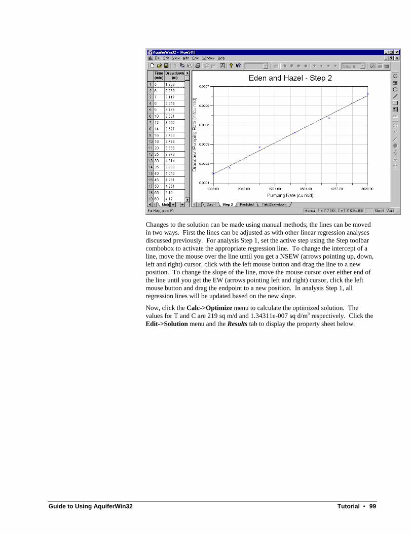
Guide to Using AquiferWin32 Tutorial • 99
Changes to the solution can be made using manual methods; the lines can be movedin two ways. First the lines can be adjusted as with other linear regression analysesdiscussed previously. For analysis Step 1, set the active step using the Step toolbarcombobox to activate the appropriate regression line. To change the intercept of aline, move the mouse over the line until you get a NSEW (arrows pointing up, down,left and right) cursor, click with the left mouse button and drag the line to a newposition. To change the slope of the line, move the mouse cursor over either end ofthe line until you get the EW (arrows pointing left and right) cursor, click the leftmouse button and drag the endpoint to a new position. In analysis Step 1, allregression lines will be updated based on the new slope.
Now, click the Calc->Optimize menu to calculate the optimized solution. Thevalues for T and C are 219 sq m/d and 1.34311e-007 sq d/m5 respectively. Click theEdit->Solution menu and the Results tab to display the property sheet below.

100 • Tutorial Guide to Using AquiferWin32
An alternative view of the “goodness of fit” is contained in the Predicted view tab.The graph, shown below, was adjusted from the default by changing the axes tolinear, changing the labels, etc. It is a useful interpretive aid and allows you toestablish the accuracy of the fit of the results by comparing observed and predicteddrawdown versus time.
Another graph presented in the Yield/Drawdown tab predicts the drawdown createdby pumping at a given rate and over a specified time. The time is currently taken tobe the average of the time of each step, equal to 180 minutes in this example. Thedrawdown line (shown in black on the graph) of the yield/drawdown curve shows thetotal drawdown/yield relationship for the given time, while the second line shows theeffect of aquifer loss (shown in red on the graph) giving the hypothetical relationship

Guide to Using AquiferWin32 Tutorial • 101
for a 100% efficient borehole. The curve is useful in evaluating the extent ofturbulent losses. The enhanced graph is shown below.

102 • Tutorial Guide to Using AquiferWin32
Analytical Flow Model
What you will learn:
• performing an analytical flow model
• plotting simulated drawdown contours
• plotting simulated hydrographs at wells
• setting up a transient simulation with variable pumping rates
• automatically calibrating the model to observed target heads
• adding a legend to the contour map with a color flood bar
The Modeling version of AquiferWin32 can also be used to perform analytical flowmodels or analyze multiple pumping well aquifer tests. The analytical elementssupported by a specific model are specified in the model specific documentation andhelp file. In general, all models support wells and targets which is what we will usein this tutorial. Additionally, some models support steady-state calculations, somesupport transient calculations and some support both.
First, use the File->New menu and create an “AquiferWin32 Flow Model”document. The only visible object on the view is an arrow. This arrow is thereference head arrow used to define the uniform flow field from which to subtract thedrawdown predicted by the analysis. The first thing to do is set up the units byclicking the mouse within the map and then using the Edit->Units menu. Select“min” for Time Units, “ft” for Length Units, “gal/min” for Pumping Rate Units and“sq ft/d” for Transmissivity Units. Click the Save As Defaults and Apply Globallycheck-boxes and accept the property sheet by clicking the OK button. It is importantto save your selections as the defaults because these values are used whenever newitems are created within the document.
Next, we need to define the map window within which you are going to work. In thiscase, click the mouse within the map window and use the File->Map menu to importthe file example.map. This file represents a large site; however we are going to focusour attention on a subset of this map. Click the Options->Map->Window menu anddrag a rectangle on the map. On the Map Window dialog that is displayed, enter“40000” for Origin X, “4200” for Origin Y, “2000” for Height and “3000” for Width.Accept the dialog by clicking the OK button. When asked to adjust the contourwindow to the new map windows, select the YES button.
Now, we need to define the initial heads for the model. To edit the parameters clickthe Edit->Reference Head menu. Set the value of Head to be “200”, Gradient to be“.001”, Angle to be “135”, X to be “37351” and Y to be “8280”. This reference headlocation is not located on the map window we are using but it serves to calculate thecorrect initial head distribution for this simulation.
Instead of using the Add->Well menu to add wells to the map, click on the Edit->Analytic Elements menu to display the AnalyticElement Information propertysheet. Set the Item Type to “Well Object” and click the Add button. The WellInformation property sheet is displayed to set the pertinent parameters for the well.On the Well Information property sheet set Well to “PW1”, X to “41250”, Y to“5100” and click the Transient Pumping Rate radio button. Click the Display tab

Guide to Using AquiferWin32 Tutorial • 103
and click the Display Label check-box. Now click the Transient tab and import thefile pw1gpm.dat to set the pumping schedule for this well. Accept the property sheetby clicking the OK button. Repeat the procedure to enter PW2 with an x-coordinateof 40750, a y-coordinate of 5100 and import the pumping schedule in filepw2gpm.dat. Accept the Analytic Element Information property sheet by clicking theOK button.
Now that we have set up two wells with variable pumping rates, click the Edit->FlowModel menu and set the solution to “Theis, 1935 (Confined)”. Click the Parameterstab and set Transmissivity to “600”, the Storage Coefficient to “.005”, the AquiferThickness to “100” and the Porosity to “.3”. The aquifer thickness and porosityparameters are used during particle tracking but not during calculation of hydraulichead. Accept the property sheet by clicking the OK button and the view shouldappear as below.
Notice that the view tabs have changed to Step 1, Step 2… This reflects that fact thatthis solution does not support direct calculation of steady state conditions and thecalculation was automatically changed to transient. Click the Options->Transientmenu to set up the time steps for the simulation. Click the Time Steps tab and fill itout as below.

104 • Tutorial Guide to Using AquiferWin32
Accept the property sheet and you will be asked if you would like to recalculate themodel. Click Yes to proceed with the recalculation. Click the Options->Contour->Parameters menu and set X Nodes to “100”, Y Nodes to “100”. Go to the Levelstab and set Minimum Level to “203” and Interval to “.5”. Now go to the Labels taband click on the Font button. Set the Size to “10” and the Font Style to “Bold”. Alsoset the value of Distance between to “500” and the Precision to “1”. Accept theproperty sheet by clicking OK. Click the Yes button to recalculate and click the Yesbutton to propagate the changes to all time steps.
The model is now calculated generating 5 view tabs representing the 5 time stepspreviously defined. The rightmost status bar cell displays the time represented by thecontour map in minutes. The contour map for Step 5 is displayed below.

Guide to Using AquiferWin32 Tutorial • 105
The next step is to calibrate the model to observed heads. Click the Add->Targetmenu and add a target between the two wells. Set the Target Designator to “MW1”,X to “41000”, Y to “5300” and click the Transient Target Head radio button. Next,click the Transient tab and import the file mw1.dat. Click the Add->Target menuand add another target between the two wells. Set the Target Designator to “MW2”,X to “41000”, Y to “5100” and click the Transient Target Head radio button. Next,click the Transient tab and import the file mw2.dat.
Now that we have set head targets to calibrate the model we can check how well ourinitial estimates of parameters match. Click the Edit->Simulation menu to thedefine the well and targets for which predicted calculations are to be performed.Using the context menu, activated by the right mouse click, use the Select All menufollowed by the Delete menu. Now import the file simtimes.dat to import the timesat which we want to calculate predicted heads. The default values do not really workin this example because we want increased time resolution in the time periods duringwhich pumping rate changes are occurring. Go to the Wells tab, click the Addbutton twice to move MW1 and MW2 from the Available Wells list to the MonitoredWells list. Accept the property sheet by clicking the OK button. No click the Calc->Recalculate menu to recalculate the model. To view the graphs for the monitoredwells, click the View->Well Data menu. Click the left-pointing arrow in the lowerleft corner of the map view to slide the tabs and reveal the MW1 and MW2 tabs.
Go the MW1 tab and click the Edit->Graph menu, click the Y-Axis tab and changethe Axis Type radio button to Arithmetic Scale and the Axis Numbers Format to“FIXED”. Also, change the Y-Axis label to “Hydraulic Head” because our model isset to calculate hydraulic head instead of drawdown. Repeat the procedure for theMW2 tab.
Notice that the observed and predicted heads do not match very well based on theinitial estimates of the parameters. To quantify the match, use the Calc->TargetStatistics menu to activate the Target Statistics Information property sheet. Theresidual standard deviation is .7. Now we will perform an optimization to estimateparameter values that best match the target values. Now take a look at the MW1 andMW2 view tabs to see the visual difference and click the Calc->Target Statistics

106 • Tutorial Guide to Using AquiferWin32
menu to quantify the match. In this case, the standard deviation is .0005 andrepresents a significantly better calibration.
After autocalibration, the next logical step is to enhance the graphical output. Clickon the Step 5 view tab to display the hydraulic head contour map for time step 5.Click the Add->Legend menu and drag a rectangle in the lower right corner of themap. Set X1 to “41700”, Y1 to “4275”, X2 to “42900” and Y2 to “5175”. Click theContents tab and set Type to “Solid” the change to the Contents tab. Set Item Typeto “Legend Object” and click the Add button. Set X1 to “900”, Y1 to “50”, X2 to“950” and Y2 to “550”. Click the Items tab and set the Automatic Maintenance ofColor Flood Legend check-box. Basically, we are reserving space within the legendto display a labeled color bar for a color flood. Accept the property sheet by clickingthe OK button. Set the Item Type to “Title Object” and click the Add button. Set Xto “900”, Y to “600” and Title to “Head (ft)”. Click the Font button and set the Sizeto “8”. Accept the dialog and property sheet by clicking the respective OK buttons.Add another title with an X of “500”, Y of “750”, Title of “LEGEND”, and set thefont to 12 point bold. Change the Item Type to “Parameter” and click the Addbutton. Set X to “50”, Y to “400” and set the list control to “Transmissivity” under“Model Parameters”. Click the Font button and set the Size to “8” and the Font styleto “Bold”. Accept the Parameter Information property sheet by clicking the OKbutton.
Add another parameter and set X to “50”, Y to “300” and set the list control to“Storage Coefficient” under “Model Parameters”. Click the Units check-box tounset it. Set the Format to “EXPONENT”. Click the Font button and set the Size to“8” and the Font style to “Bold”. Accept the Parameter Information property sheetby clicking the OK button. Add a final parameter and set X to “50”, Y to “100” andset the list control to “Time” under “Contour Parameters”. Click the Font button andset the Size to “8” and the Font style to “Bold”. Accept the Parameter Informationproperty sheet by clicking the OK button. Now accept the Legend Informationproperty sheet by clicking the OK button.
Now that a legend is displayed, click the View->Display Color Flood menu and theresulting contour map is displayed below.

Guide to Using AquiferWin32 Tutorial • 107