TUTORIAL IN BIOSTATISTICS DEVELOPMENT OF A CLINICAL ...lcc.uma.es/~jja/recidiva/064.pdf · and Etiological Agents of Pneumonia, Sepsis and Meningitis in Young Infants FRANK E. HARRELL,

*Correspondence to: Frank E. Harrell Jr, PhD, Box 600, Health Sciences Center, University of Virginia, CharlottesvilleVA 22908, U.S.A. E-mail: [email protected]

Contract grant sponsor: Agency for Health Care Policy and Research; contract grant number: HS-06830, HS-07137

CCC 0277—6715/98/080909—36$17.50( 1998 John Wiley & Sons, Ltd.

STATISTICS IN MEDICINE

Statist. Med. 17, 909—944 (1998)

TUTORIAL IN BIOSTATISTICS

DEVELOPMENT OF A CLINICAL PREDICTION MODELFOR AN ORDINAL OUTCOME:

The World Health Organization Multicentre Study of Clinical Signsand Etiological Agents of Pneumonia, Sepsis and Meningitis

in Young Infants

FRANK E. HARRELL, Jr.1*, PETER A. MARGOLIS2, SANDY GOVE3, KAREN E. MASON3,E. KIM MULHOLLAND4, DEBORAH LEHMANN5, LULU MUHE6,

SALVACION GATCHALIAN7 AND HEINZ F. EICHENWALD8and the

WHO/ARI YOUNG INFANT MULTICENTRE STUDY GROUP

1 Division of Biostatistics and Epidemiology, Department of Health Evaluation Sciences, University of Virginia, Charlottesville,U.S.A.

2 The Division of Community Pediatrics, University of North Carolina, Chapel Hill, U.S.A.3 Programme for the Control of Acute Respiratory Infection (ARI) of the World Health Organization, Geneva, Switzerland

4 MRC, The Gambia5 Papua New Guinea Institute of Medical Research, Goroka

6 Department of Paediatrics and Child Health, Addis Ababa University, Ethiopia7 Research Institute for Tropical Medicine, Alabang, Philippines

8 Department of Pediatrics, University of Texas Southwestern Medical Center, Dallas, U.S.A.

SUMMARY

This paper describes the methodologies used to develop a prediction model to assist health workers indeveloping countries in facing one of the most difficult health problems in all parts of the world: thepresentation of an acutely ill young infant. Statistical approaches for developing the clinical predictionmodel faced at least two major difficulties. First, the number of predictor variables, especially clinical signsand symptoms, is very large, necessitating the use of data reduction techniques that are blinded to theoutcome. Second, there is no uniquely accepted continuous outcome measure or final binary diagnosticcriterion. For example, the diagnosis of neonatal sepsis is ill-defined. Clinical decision makers must identifyinfants likely to have positive cultures as well as to grade the severity of illness. In the WHO/ARI YoungInfant Multicentre Study we have found an ordinal outcome scale made up of a mixture of laboratory anddiagnostic markers to have several clinical advantages as well as to increase the power of tests for riskfactors. Such a mixed ordinal scale does present statistical challenges because it may violate constant slope

assumptions of ordinal regression models. In this paper we develop and validate an ordinal predictive modelafter choosing a data reduction technique. We show how ordinality of the outcome is checked against eachpredictor. We describe new but simple techniques for graphically examining residuals from ordinal logisticmodels to detect problems with variable transformations as well as to detect non-proportional odds andother lack of fit. We examine an alternative type of ordinal logistic model, the continuation ratio model, todetermine if it provides a better fit. We find that it does not but that this model is easily modified to allow theregression coefficients to vary with cut-offs of the response variable. Complex terms in this extended modelare penalized to allow only as much complexity as the data will support. We approximate the extendedcontinuation ratio model with a model with fewer terms to allow us to draw a nomogram for obtainingvarious predictions. The model is validated for calibration and discrimination using the bootstrap. We applymuch of the modelling strategy described in Harrell, Lee and Mark (Statist. Med. 15, 361—387 (1998)) forsurvival analysis, adapting it to ordinal logistic regression and further emphasizing penalized maximumlikelihood estimation and data reduction. ( 1998 John Wiley & Sons, Ltd.

1. INTRODUCTION

The presentation of an acutely ill young infant presents health workers in all parts of the worldwith one of their most difficult problems. Serious infections are the main cause of morbidity andmortality in infants under 3 months of age in developing countries. Diagnosis is difficult— meningitis or pneumonia might appear as clear clinical syndromes, but more often the picture ismixed and the infant is labelled as ‘sepsis’. Even in industrialized countries, treatment is usuallybased on clinical impressions supported by laboratory data, which by itself is often inconclusive.In developing countries, clinical signs are the only tools available in most places. The ability todetect serious bacterial infection early in young infants is important in defining appropriateprevention and treatment strategies. A better clinical prediction rule to be used by peripheralhealth workers might result in more appropriate referral to hospital as well as less antibiotic usein very low-risk infants.

We set out to determine which combination of clinical signs most accurately predict the groupof infants who have meningitis, sepsis or pneumonia. There is no single ‘gold standard’ againstwhich to correlate these signs. It is tempting to use as an endpoint the physician’s expert clinicaldiagnosis. This would induce a circularity which would inflate the predictive discrimination of theprediction model, because clinical signs are major determinants of the overall clinical impression.Death is the only endpoint that can be ascertained for every infant, but truly ill infants who weresuccessfully treated early with antibiotics may not die.

Even without a gold standard, however, there are a number of generally agreed laboratory testswhich could be used to construct a reasonable outcome scale, including cerebro-spinal fluid(CSF) culture from a lumbar puncture (LP), blood culture (BC), arterial oxygen saturation (SaO

2,

a measure of lung function), and chest X-ray (CXR). In this study, 249 infants died, and deathcould be placed at the top of an ordinal outcome scale. Many of the deaths were related tostarting treatment too late so they were not preventable with antibiotics. For this paper, wechoose to ignore death (but not to exclude patients who died) when constructing the scale as themain goal was to predict treatable disease. Ignoring death resulted in some of the clinical signsbeing stronger predictors. Two-thirds of the deaths were redistributed to other positive outcomecategories.

We model an ordinal outcome scale using the proportional odds (PO) form of an ordinallogistic model1 and the forward continuation ratio (CR) ordinal logistic model.2 (see references3—18 for some excellent background references, applications, and extensions to the ordinal

910 F. HARRELL E¹ A¸.

Statist. Med. 17, 909—944 (1998)( 1998 John Wiley & Sons, Ltd.

models.) We predicted this ordinal outcome using clinical symptoms, signs, and basic variablessuch as age, weight, temperature and respiratory rate. Nine major statistical problems had to beaddressed in these analyses:

1. How does one avoid estimating a separate coefficient for the large number of clinical signs?(Overfitting and poor model validation would result if all signs were treated as separatecandidate variables in the model.)19

2. Can expert clinicians assign weights for signs a priori that adequately predict the outcomes?3. Given that the clinical signs can be combined in meaningful ways, how should a cluster of such

variables be quantified? Should weights for multiple signs be summed or should the cluster bescored using the weight associated with the most severe sign present? Is the union of all signs(that is, presence of any sign) within a cluster an adequate summary of that cluster?

4. How can continuous predictors such as respiratory rate or temperature be modelled flexiblywithout assuming linearity?

5. Since the response variable is a hierarchical assignment made up of disparate measurements isthe proportional odds assumption likely to be violated?

6. Will another type of ordinal logistic model provide a better fit?7. How can the constant slopes assumption be relaxed without causing overfitting?8. How does one diagram the final ordinal model so that field health workers can quickly obtain

predicted risks of various severities of outcome?9. How does one validate an ordinal regression model without sacrificing sample size?

Section 2 gives a brief overview of the World Health Organization/Acute Respiratory Infection(WHO/ARI) Multicentre Study design. Section 3 provides the definition of the ordinal outcomescale. In Section 4 we discuss how clinical signs were scored (individually) and clustered. Section 5tests the adequacy of weights specified by subject-matter specialists and depicts the utility ofvarious scoring schemes using a tentative ordinal logistic model. Section 6 depicts a simple way toassess the assumption of ordinality of the response with respect to each predictor, and to examinethe PO and CR assumptions separately for each predictor. In section 7 we derive a tentativeproportional odds model using cluster scores and using regression splines to allow otherpredictors to be flexibly related to the log odds of an outcome. Section 8 shows how residualsfrom binary logistic models can be adapted to the ordinal case, and uses smoothed residual plotsto assess the proportional odds assumption with respect to each predictor. Section 9 examines thefit of a continuation ratio model. Section 10 shows how the CR model can easily be extended (andfitted using standard software) to allow some or all of the regression coefficients to vary withcut-offs of the response level as well as to provide formal tests of constant slopes. Section 11 showshow penalized maximum likelihood estimation is used to improve future predictive accuracy. InSection 12 the full model is approximated by a sub-model, and a nomogram is constructed for theapproximate model. Section 13 demonstrates how the ordinal model is validated using thebootstrap. Many of the methods discussed here were discussed in Harrell et al.20 where the focuswas on survival analysis. This modelling strategy used here generally follows that paper, withadditional stress on penalized estimation.

Cole et al.17 also presented a case study in developing a PO ordinal logistic model fordiagnosing illness in infants under 6 months of age. In their study, which was based on patientswho were less severely ill than those in the present study, the ordinal outcome was physicians’subjective assessment of the severity of illness. The analysis was based on stepwise variableselection of individual clinical signs which would be expected to prevent the model calibration to

CLINICAL PREDICTION MODEL FOR AN ORDINAL OUTCOME 911


*Some mothers refused having blood drawn for their children, adding a slight bias to the remaining sampled group whichmade them slightly more sick. At one site, the sample was systematic (every fifth patient) but sampling was done moreoften when mothers refused to participate

be accurate for very low and very high risk infants. That paper included a nice example ofoptimally rounding regression coefficients so that a simple severity score could be derived.

For almost all steps of the analysis, computer code is shown, both to make the steps moreconcrete as well as to show their feasibility. All analyses were done using S-plus version 3.221 onUNIX using Sun Sparcstation 2 and 10 computers in conjunction with the Design libraryof UNIX and Microsoft Windows S-plus functions.22 For binary and PO logistic modelsDesign has a general penalized maximum likelihood estimation facility in the lrm function.It also has a function cr.setup which allows the CR model to be fitted in an extremelyflexible way using a binary logistic model on a modified input data set. Design is available athttp://www.med.virginia.edu/medicine/clinical/hes/biostat.htm. varclus, transcan, impute,and scat1d are separate functions in the Hmisc library in statlib, also written by the first author.

2. STUDY DESIGN

The WHO/ARI Multicentre Study of Clinical Signs and Etiological Agents of Pneumonia, Sepsisand Meningitis in Young Infants was undertaken in Ethiopia, The Gambia, Papua New Guinea,and the Phillippines to collect data that would allow better screening criteria to be derived forfinding infants at high risk of serious infection.23 Standardized laboratory and clinical evalu-ations (clinical history, risk factors such as low birth weight, CXR, SaO

2, BC, LP etc.) were done.

Infants brought for primary care were enrolled if any of the following were present: cough;difficult, fast or noise breathing; fever or hypothermia; not feeding well (less than half of normalintake); abnormally sleepy or difficult to wake; convulsions; rectal temperature *37)5°C or)35)5°C; or mother volunteered that the baby was very sick, irritable, or has stopped breathingor turned blue/black. Infants were excluded if the illness began in hospital (except for delivery),the clinic visit was for trauma, burn, or routine care such as immunization, weight (1500 gduring the first 48 hours of life, there was a documented episode of previous pneumonia, sepsis, ormeningitis within the last 3 weeks, if an obvious congenital malformation was present, or if theinfant had previously been enrolled in the study. 8418 infants were screened and the 4552 havinga positive symptom without an exclusion were enrolled.

To be a candidate for BC and CXR, an infant had to have a clinical indication for one of thethree diseases, according to prespecified criteria in the study protocol (n"2398). Blood work-up(but not LP) and CXR was also done on a random sample intended to be 10 per cent of infantshaving no signs or symptoms suggestive of infection (n"175).* Infants with signs suggestive ofmeningitis had LP. All 4552 infants received a full physical exam and standardized pulse oximetryto measure SaO

2. The vast majority of infants getting CXR had the X-rays interpreted by three

independent radiologists.For determining outcomes, BC was considered positive if the blood culture was definite or

probable for bacterial infection.23 CSF was positive if the CSF culture was positive or there weremore than 10 white cells in the CSF, after a correction was made for a bloody tap. CXR is positiveif all radiologists who read the CXR and ruled it interpretable classified the infant’s X-ray asdefinitely or probably abnormal.



*Proportion of deaths for BC#, BC!, CSF#, CSF!, SaO2(90 per cent, SaO

2*90 per cent were, respectively,

0)30, 0)08, 0)29, 0)05, 0)25, 0)04

Table I. Ordinal outcome scale

Outcome Definition n Fraction in outcome levellevel ½

BC, CXR Not Randomindicated indicated sample*

4552 (n"2398) (n"1979) (n"175)

0 None of the above 3551 0)63 0)96 0)911 90%)SaO

2(95% or CXR# 490 0)17 0)04s 0)05

2 BC# or CSF# or SaO2(90% 511 0)21 0)00t 0)03

*A separate sample of patients not indicated for laboratory work-up but having it anywaysSaO

2was measured but CXR was not done

tAssumed zero since neither BC nor LP were done

The analyses which follow are not corrected for verification bias24 with respect to BC, LP andCXR, but Section 3 has some data describing the extent of the problem.

3. ORDINAL OUTCOME SCALE

Rationale and details of the outcome scale construction are found in a background paper.25 Asdiscussed by Follman,26 it is useful to derive new outcome variables (risk scores) by observinghow non-fatal events predict death. We followed this scheme but extended it with a two-stagestrategy. First, we found that the more important non-fatal response measures, BC#, CSF#,and severe hypoxemia (SaO

2(90 per cent, altitude adjusted), had roughly equal weight in

predicting death* so the union of these findings was used as the top outcome level. Next, CXRand moderate hypoxemia (90(SaO

2(95 per cent) were examined for their association with the

probability that the patient had BC# or CSF#. These two markers were found to have thesame associations with this worse outcome (probabilities of BC#XCSF# were equal for CXR#and for SaO

23[90 per cent, 95 per cent), and were lower but equal for CXR! and SaO

2*95

per cent).Patients were then assigned to the worst qualifying outcome category. Table I shows the

definition of the ordinal outcome variable ½ and shows the distribution of ½ by the laboratorywork-up strategy.

The effect of verification bias is a false negative fraction of 0)03 for ½"2, from comparing thedetection fraction of zero for ½"2 in the ‘not indicated’ group with the observed positivefraction of 0)03 in the random sample that was fully worked up. The extent of verification bias in½"1 is 0)05!0)04"0)01. In what follows, these biases will be ignored.

4. VARIABLE CLUSTERING

Expert clinical judgement was used to enumerate a list of clinical variables to collect, including 47clinical signs. The list reflects the content of an expert paediatric examination. As a first step in



coding the predictor variables, all questionnaire items that were connected (for example, usingskip rules such as ‘if condition was present, what was its severity?’) were scored as a single variableusing equally spaced codes, with 0—3 representing, for example, sign not present, mild, moderate,severe. The resulting list of clinical signs with their abbreviations is given in Table II. The signs areorganized into clusters as will be discussed below. Here, hx stands for history, ausc forauscultation, and hxprob for history of problems. Two signs (qcr, hcm) were listed twice becausethey were later placed into two clusters each.

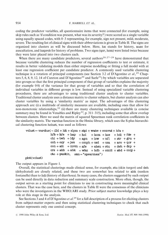
When there are many candidate predictors, several authors20,27~29 have demonstrated thatbecause variable clustering reduces the number of regression coefficients to test or estimate, itresults in better validating models than either stepwise modelling or fitting a full model with atleast one regression coefficient per candidate predictor. A commonly used variable clusteringtechnique is a rotation of principal components (see Section 3.2 of D’Agostino et al.,29 Chap-ters 5, 6, 8, 9, 12, 14 of Cureton and D’Agostino30 and Sarle31) by which variables are separatedinto groups so that the first principal component of that group of variables explains the majority(for example 0)8) of the variance for that group of variables and so that the correlation ofindividual variables in different groups is low. Instead of using specialized variable clusteringprocedures, there are advantages to using traditional cluster analysis to cluster variables.Traditional cluster analysis uses a distance matrix to cluster subjects, but cluster analysis can alsocluster variables by using a ‘similarity matrix’ as input. The advantages of this clusteringapproach are: (i) a multitude of similarity measures are available, including ones that allow fornon-monotonic relationships,32 (ii) there are many clustering techniques available (a concisesummary may be found in Venables and Ripley33, p. 311—315), including some that allow overlapbetween clusters. Here we used the matrix of squared Spearman rank correlation coefficients inthe similarity matrix. The varclus function in the Hmisc library, which uses the S-plus hierarchi-cal clustering function hclust, was used as follows:

The output appears in Figure 1.Overall, the statistical clusterings made clinical sense, for example, stu (skin turgor) and deh

(dehydrated) are closely related, and these two are somewhat less related to abk (sunkenfontanelle) than to hdi (history of diarrhoea). In many cases, the clusters suggested by such outputcan be used directly in data reduction and summary scale construction. More often, though, theoutput serves as a starting point for clinicians to use in constructing more meaningful clinicalclusters. That was the case here, and the clusters in Table II were the consensus of the clinicianswho were the investigators in the WHO/ARI study. Prior subject matter knowledge plays a keyrole at this stage in the analysis.

See Sections 3 and 4 of D’Agostino et al.29 for a full description of a process for eliciting clustersfrom subject-matter experts and then using statistical clustering techniques to check that eachcluster represents only one central concept.



Table II. Clinical signs

Cluster name Sign abbreviation Name of sign Values

bul.conv abb bulging fontanelle 0—1convul hx convulsion 0—1

hydration abk sunken fontanelle 0—1hdi hx diarrhoea 0—1deh dehydrated 0—2stu skin turgor 0—2dcp digital capillary refill 0—2

drowsy hcl less activity 0—1qcr quality of crying 0—2csd drowsy state 0—2slpm sleeping more 0—1wake wakes less easy 0—1aro arousal 0—2mvm amount of movement 0—2

agitated hcm crying more 0—1slpl sleeping less 0—1con consolability 0—2csa agitated state 0—1

crying hcm crying more 0—1hcs crying less 0—1qcr quality of crying 0—2smi2 smiling ability]age'42 days 0—2

reffort nfl nasal flaring 0—3lcw lower chest in-drawing 0—3gru grunting 0—2ccy central cyanosis 0—1

stop.breath hap hx stop breathing 0—1apn apnoea 0—1

ausc whz wheezing 0—1coh cough heard 0—1crs crepitation 0—2

hxprob hfb fast breathing 0—1hdb difficulty breathing 0—1hlt mother report respiratory problems none, chest, other

feeding hfa hx abnormal feeding 0—3absu sucking ability 0—2afe drinking ability 0—2

labor chi previous child died 0—1fde fever at delivery 0—1ldy days in labour 1—9twb water broke 0—1

abdominal abd abdominal distension 0—4jau jaundice 0—1omph omphalitis 0—1

fever.ill illd ge-adjusted number days illhfe hx fever 0—1

pustular conj conjuctivitis 0—1oto otoscopy impression 0—2puskin pustular skin rash 0—1



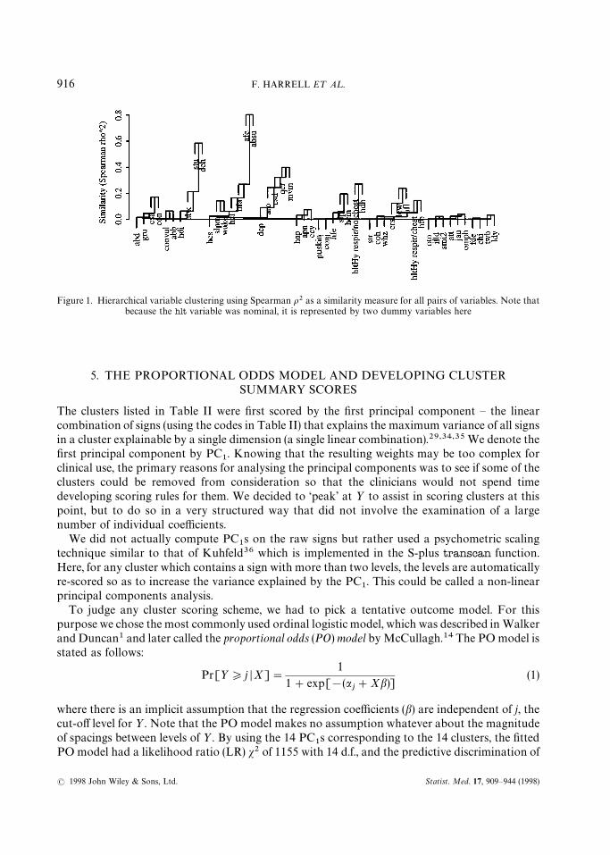
Figure 1. Hierarchical variable clustering using Spearman o2 as a similarity measure for all pairs of variables. Note thatbecause the hlt variable was nominal, it is represented by two dummy variables here

5. THE PROPORTIONAL ODDS MODEL AND DEVELOPING CLUSTERSUMMARY SCORES

The clusters listed in Table II were first scored by the first principal component — the linearcombination of signs (using the codes in Table II) that explains the maximum variance of all signsin a cluster explainable by a single dimension (a single linear combination).29,34,35 We denote thefirst principal component by PC

1. Knowing that the resulting weights may be too complex for

clinical use, the primary reasons for analysing the principal components was to see if some of theclusters could be removed from consideration so that the clinicians would not spend timedeveloping scoring rules for them. We decided to ‘peak’ at ½ to assist in scoring clusters at thispoint, but to do so in a very structured way that did not involve the examination of a largenumber of individual coefficients.

We did not actually compute PC1s on the raw signs but rather used a psychometric scaling

technique similar to that of Kuhfeld36 which is implemented in the S-plus transcan function.Here, for any cluster which contains a sign with more than two levels, the levels are automaticallyre-scored so as to increase the variance explained by the PC

1. This could be called a non-linear

principal components analysis.To judge any cluster scoring scheme, we had to pick a tentative outcome model. For this

purpose we chose the most commonly used ordinal logistic model, which was described in Walkerand Duncan1 and later called the proportional odds (PO) model by McCullagh.14 The PO model isstated as follows:

Pr[½*j DX]"1

1#exp[!(aj#Xb)]

(1)

where there is an implicit assumption that the regression coefficients (b) are independent of j, thecut-off level for ½. Note that the PO model makes no assumption whatever about the magnitudeof spacings between levels of ½. By using the 14 PC

1s corresponding to the 14 clusters, the fitted

PO model had a likelihood ratio (LR) s2 of 1155 with 14 d.f., and the predictive discrimination of



*See reference 20 for details; Dxy"2(c!1

2) where c is the probability of concordance between pairs of XbK and ½ values,

which is a generalization of a receiver operating characteristic curve area

Table III. Clinician combinations, rankings and scorings of signs

Cluster Combined/ranked signs in order of severity Weights

bul.conv abbXconvul 0—1drowsy hcl, qcr'0, csd'0XslpmXwake, aro'0, mvm'0 0—5agitated hcm, slpl, con"1, csa, con"2 0, 1, 2, 7, 8, 10refort nfl'0, lcw'1, gru"1, gru"2, ccy 0—5ausc whz, coh, crs'0 0—3feeding hfa"1, hfa"2, hfa"3, absu"1Xafe"1, absu"2Xafe"2 0—5abdominal jauXabd'0Xomph 0—1

the clusters was quantified by a Somers’ Dxy

rank correlation between XbK and ½ of 0)596.* Thefollowing clusters were not statistically important predictors and we assumed that the lack ofimportance of the PC

1s in predicting½ (adjusted for the other PC

1s) justified a conclusion that no

sign within that cluster was clinically important in predicting ½: hydration, hxprob, pustular,crying, fever.ill, stop.breath, labor. This list was identified using a backward step-down pro-cedure on the full model. The total Wald s2 for these 7 PC

1s was 22)4 (P"0)002). The reduced

model had LR s2"1133 with 7 d.f., Dxy"0)591. The bootstrap validation in Section 13 penaliz-

ed for fitting the 7 predictors.During a meeting of the study group, the clinicians were asked to rank the clinical severity of

signs within each potentially important cluster. During this step, the clinicians also rankedseverity levels of some of the component signs, and some cluster scores were simplified, especiallywhen the signs within a cluster occurred infrequently. The clinicians also assessed whether theseverity points or weights should be equally spaced, assigning unequally spaced weights for onecluster (agitated). The resulting rankings and sign combinations are shown in Table III. The signsor sign combinations separated by a comma are treated as separate categories, whereas somesigns were unioned (‘or’-ed) when the clinicians deemed them equally important. As an example, ifan additive cluster score was to be used for drowsy, the scorings would be 0"none present,1"hcl, 2"qcr'0, 3"csd'0 or slpm or wake, 4"aro'0, 5"mvm'0 and the scoreswould be added.

This table reflects some data reduction already (unioning some signs and selection of levels ofordinal signs) but more reduction is needed. Even after signs are ranked within a cluster, there arevarious ways of assigning the cluster scores. We investigated six methods. We started with thepurely statistical approach of using PC

1to summarize each cluster. Second, all sign combinations

within a cluster were unioned to represent 0—1 cluster score. Third, only sign combinationsthought by the clinicians to be severe were unioned, resulting in drowsy"aro'0 or mvm'0,agitated"csa or con"2, reffort"lcw'1 or gru'0 or ccy, ausc"crs'0, and feeding"absu'0or afe'0. For clusters that are not scored 0—1 in Table III, the fourth summarization method wasa hierarchical one which used the weight of the worst applicable category as the cluster score. Forexample, if aro"1 but mvm"0, drowsy would be scored as 4. The fifth method counted thenumber of positive signs in the cluster. The sixth method summed the weights of all signs or sign



Table IV. Predictive information of various cluster scoring strategies

Scoring method LR s2 d.f. AIC

PC1

of each cluster 1133 7 1119Union of all signs 1045 7 1031Union of higher categories 1123 7 1109Hierarchical (worst sign) 1194 7 1180Additive, equal weights 1155 7 1141Additive using clinician weights 1183 7 1169Hierarchical, data-driven weights 1227 25 1177

combinations present. Finally, the worst sign combination present was again used as in thesecond method, but the points assigned to the category were data driven ones obtained by usingextra dummy variables. This provides an assessment of the adequacy of the clinician-specifiedweights. By comparing rows 4 and 7 in Table IV we see that response data-driven sign weightshave a slightly worse Akaike information criterion (AIC) or LR s2!2]d.f. (which penalizes themodel for complexity37), indicating that the number of extra b parameters estimated was notjustified by the improvement in s2. The hierarchical method, using the clinicians’ weights,performed quite well. The only cluster with inadequate clinician weights was ausc — see following.The PC

1method, without any guidance, performed well, as in Harrell et al.19 The only reasons

not to use it are that it requires a coefficient for every sign in the cluster and coefficients are nottranslatable into simple scores such as 0, 1,2 .

Representation of clusters by a simple union of selected signs or of all signs is inadequate, butotherwise the choice of methods is not very important in terms of explaining variation in ½. Wechose the fourth method, a hierarchical severity point assignment (using weights which wereprespecified by the clinicians), for its ease of use and of handling missing component variables (inmost cases) and potential for speeding up the clinical exam (examining to detect more importantsigns first). Because of what was learned regarding the relationship between ausc and ½, wemodified the ausc cluster score by redefining it as ausc"crs'0 (crepitations present). Note thatneither the ‘tweaking’ of ausc nor the examination of the seven scoring methods displayed inTable IV will be taken into account in the model validation.

One attractive alternative approach that we did not try was the battery reduction strategydescribed in Chapter 12 of Cureton and D’Agostino30 in which one finds a subset of the variablesin each cluster whose PC

1adequately represents the whole cluster’s PC

1.

6. ASSESSING ORDINALITY OF ½ FOR EACH X, AND UNADJUSTEDCHECKING OF PO AND CR ASSUMPTIONS

A basic assumption of all commonly used ordinal regression models is that the response variablebehaves in an ordinal fashion with respect to each predictor. Assuming that a predictor X islinearly related to the log odds of some appropriate event, a simple way to check for ordinality isto plot the mean of X stratified by levels of ½ (denote these by EK (X D½"y)). These means shouldbe in a consistent order. If for many of the Xs, two adjacent categories of ½ do not distinguish themeans, that is evidence that those levels of ½ should be pooled.



*For inner values of ½ in the PO models, these probabilities are differences between terms given by equation (1)

One can also estimate the mean or expected value of X D½"j given that the ordinal modelassumption hold. This is a useful tool for examining those assumptions, at least in an unadjustedfashion. For simplicity, assume that X is discrete, and let P

jx"Pr(½"j DX"x, model) be the

probability that ½"j given X"x that is dictated from the model being fitted, with X being theonly predictor in the model. Then

Pr(X"x DX"j, model)"Pr(½"j DX"x, model)Pr(X"x)/Pr(½"j )

E(X D½"j, model)"+x

xPjx

Pr(X"x)/Pr(½"j ) (2)

and the expectation can be estimated by

EK (X D½"j, model)"+x

xPKjx

fx/g

j(3)

where PKjx

denotes the estimate of Pjx

from the fitted 1-predictor model*, fx

is the frequency ofX"x in the sample of size n, and g

jis the frequency of ½"j in the sample. This estimate can be

computed conveniently without grouping the data by X. For n subjects let the n values of X bex1, x

2,2 ,x

n. Then

EK (X D½"j )"n+i/1

xiPKjxi

/gj. (4)

Figure 2 was produced by the S-plus function plot.xmean.ordinaly in the Design library, whichplots simple ½-stratified means overlaid with EK (X D½"j, model), with j on the x-axis. Here weexpect strongly non-linear effects for temp, rr and hrat, so for those predictors we plot the meanabsolute differences from suitable ‘normal’ values as an approximate solution:

par(mfrow"c(3,4)) d3]4 matrix of plotsplot.xmean.ordinaly(Y&age#abs(temp-37)#abs(rr-60)#abs(hrat-125)#

waz#bul.conv#drowsy#agitated#reffort#ausc#feeding#abdominal, cr"T)

The plot is shown in Figure 2. ½ does not seem to operate in an ordinal fashion with respect toage, Drr-60 D or ausc. For the other variables, ordinality holds, and PO holds reasonably wellexcept for bul.conv, drowsy and abdominal. For heart rate, the PO assumption appears to besatisfied perfectly. CR model assumptions appear to be no less tenuous than PO assumptions, atleast when fitting one variable at a time.

There is a relationship between score residuals defined later in equation (6) and a slightlydifferent comparison between stratified means of X and expected values under the model.Suppose that simple means and expected values were computed under the condition that ½*jinstead of the condition ½"j. Then EK (X D½*j )!EK (X D½*j, model) is proportional to themean of the score residuals for the PO model.

7. A TENTATIVE FULL PROPORTIONAL ODDS MODEL

Using summary cluster scores that were developed in Section 5, the original list of 14 clusters with47 signs was reduced to 7 predictors as listed in Table III: two unions of signs (bul.conv,



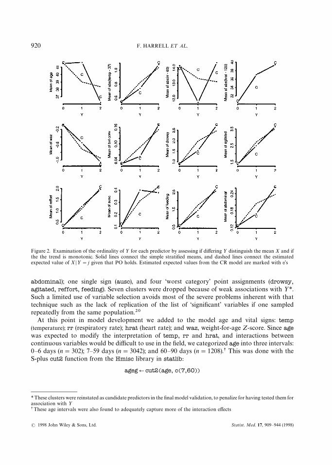
Figure 2. Examination of the ordinality of ½ for each predictor by assessing if differing ½ distinguish the mean X and ifthe the trend is monotonic. Solid lines connect the simple stratified means, and dashed lines connect the estimatedexpected value of X D½"j given that PO holds. Estimated expected values from the CR model are marked with c’s

*These clusters were reinstated as candidate predictors in the final model validation, to penalize for having tested them forassociation with ½

sThese age intervals were also found to adequately capture more of the interaction effects

abdominal); one single sign (ausc), and four ‘worst category’ point assignments (drowsy,agitated, reffort, feeding). Seven clusters were dropped because of weak associations with ½*.Such a limited use of variable selection avoids most of the severe problems inherent with thattechnique such as the lack of replication of the list of ‘significant’ variables if one sampledrepeatedly from the same population.20

At this point in model development we added to the model age and vital signs: temp(temperature); rr (respiratory rate); hrat (heart rate); and waz, weight-for-age Z-score. Since agewas expected to modify the interpretation of temp, rr and hrat, and interactions betweencontinuous variables would be difficult to use in the field, we categorized age into three intervals:0—6 days (n"302); 7—59 days (n"3042); and 60—90 days (n"1208).s This was done with theS-plus cut2 function from the Hmisc library in statlib:

agegQcut2(age, c(7,60))



*Four knots were used for hrat because it was thought to be less important a priori, and fewer were used for waz becauseit was thought to operate almost linearlysActually, the statement which produced this output is latex(anova(f1)), which typeset the output using the LAT

EX

document processing language42

The new variables temp, rr, hrat, waz were missing in, respectively, n"13, 11, 147 and 20infants. Because the three vital sign variables are somewhat correlated with each other, cus-tomized imputation models were developed to impute all the missing values without assuminglinearity or even monotonicity of any of the regressions. The S-plus transcan and imputefunctions from Hmisc were used to impute vital signs as follows:

vsign.transQtranscan(&temp#hrat#rr, imputed"T)tempQimpute(vsign.trans, temp)hrat Qimpute(vsign.trans, hrat)rr Qimpute(vsign.trans, rr)

After transcan estimated optimal restricted cubic spline transformations, temp could be pre-dicted with adjusted R2"0)17 from hrat and rr, hrat could be predicted with adjustedR2"0)14 from temp and rr, and rr could be predicted with adjusted R2 of only 0)06. The firsttwo R2, while not large, mean that customized imputations are more efficient than imputing withconstants. Imputations on rr were closer to the median rr of 48/minute as compared with theother two vital signs whose imputed values have more variation. In a similar manner, waz wasimputed using age, birth weight, head circumference, body length, and prematurity (adjusted R2

for predicting waz from the others was 0.74).The continuous predictors temp, hrat, rr were not assumed to linearly relate to the log odds

that ½*j. Flexible piecewise cubic polynomials (restricted cubic spline functions38~41 with5 knots or join points for temp, rr and 4 knots for hrat,waz* ) were used to model the effects ofthese variables, using the rcs function with the binary and PO logistic regression function lrm inthe Design library:

f1Qlrm(Y&ageg * (rcs(temp,5)#rcs(rr,5)#rcs(hrat,4))#rcs(waz,4)#bul.conv#drowsy#agitated#reffort#ausc#feeding#abdominal, x"T, y"T) dx"T, y"T used by resid( ) below

Here the asterisk in the formula indicates that main effects and interactions are to be fitted. Thismodel has LR s2 of 1393 with 45 d.f. and D

xy"0)653. Wald tests of non-linearity and interaction

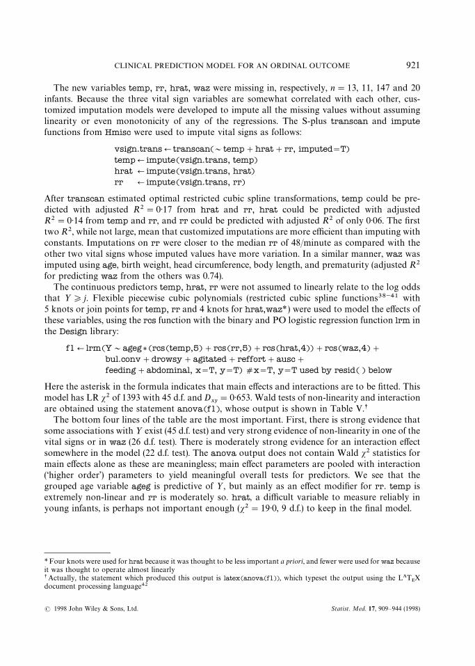
are obtained using the statement anova(f1), whose output is shown in Table V.sThe bottom four lines of the table are the most important. First, there is strong evidence that

some associations with ½ exist (45 d.f. test) and very strong evidence of non-linearity in one of thevital signs or in waz (26 d.f. test). There is moderately strong evidence for an interaction effectsomewhere in the model (22 d.f. test). The anova output does not contain Wald s2 statistics formain effects alone as these are meaningless; main effect parameters are pooled with interaction(‘higher order’) parameters to yield meaningful overall tests for predictors. We see that thegrouped age variable ageg is predictive of ½, but mainly as an effect modifier for rr. temp isextremely non-linear and rr is moderately so. hrat, a difficult variable to measure reliably inyoung infants, is perhaps not important enough (s2"19)0, 9 d.f.) to keep in the final model.



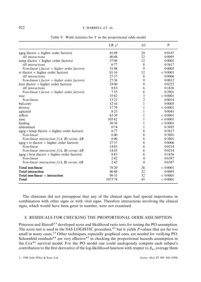
Table V. Wald statistics for ½ in the proportional odds model

LR s2 d.f. P

ageg (factor#higher order factors) 41)49 24 0)0147All interactions 40)48 22 0)0095

temp (factor#higher order factors) 37)08 12 0)0002All interactions 6)77 8 0)5617Non-linear ( factor#higher order factors) 31)08 9 0)0003

rr (factor#higher order factors) 81)16 12 (0)0001All interactions 27)37 8 0)0006Non-linear ( factor#higher order factors) 27)36 9 0)0012

hrat (factor#higher order factors) 19)00 9 0)0252All interactions 8)83 6 0)1836Non-linear ( factor#higher order factors) 7)35 6 0)2901

waz 35)82 3 (0)0001Non-linear 13)21 2 0)0014

bul.conv 12)16 1 0)0005drowsy 17.79 1 (0)0001agitated 8)25 1 0)0041reffort 63)39 1 (0)0001ausc 105)82 1 (0)0001feeding 30)38 1 (0)0001abdominal 0)74 1 0)3895ageg]temp (factor#higher order factors) 6)77 8 0)5617

Non-linear 6)40 6 0)3801Non-linear interaction: f (A, B) versus AB 6)40 6 0)3801

ageg]rr (factor#higher order factors) 27)37 8 0)0006Non-linear 14)85 6 0)0214Non-linear interaction: f (A, B) versus AB 14.85 6 0)0214

ageg]hrat (factor#higher order factors) 8)83 6 0)1836Non-linear 2)42 4 0)6587Non-linear interaction: f (A, B) versus AB 2)42 4 0)6587

Total non-linear 78)20 26 (0)0001Total interaction 40)48 22 0)0095Total non-linear#interaction 96)31 32 (0)0001Total 1073)78 45 (0)0001

The clinicians did not presuppose that any of the clinical signs had special importance incombination with other signs or with vital signs. Therefore interactions involving the clinicalsigns, which would have been great in number, were not examined.

8. RESIDUALS FOR CHECKING THE PROPORTIONAL ODDS ASSUMPTION

Peterson and Harrell15 developed score and likelihood ratio tests for testing the PO assumption.The score test is used in the SAS LOGISTIC procedure,43 but it yields P-values that are far toosmall in many cases.15 Other techniques, especially graphical ones, are needed for verifying PO.Schoenfeld residuals44 are very effective45 in checking the proportional hazards assumption inthe Cox46 survival model. For the PO model one could analogously compute each subject’scontribution to the first derivative of the log-likelihood function with respect to b

m, average them



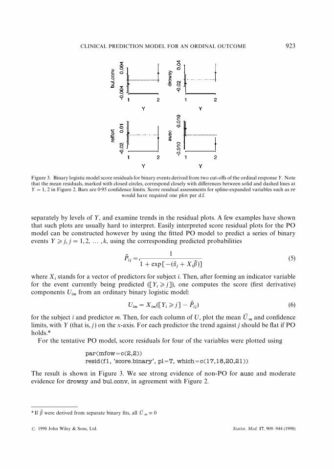
Figure 3. Binary logistic model score residuals for binary events derived from two cut-offs of the ordinal response½. Notethat the mean residuals, marked with closed circles, correspond closely with differences between solid and dashed lines at½"1, 2 in Figure 2. Bars are 0)95 confidence limits. Score residual assessments for spline-expanded variables such as rr

would have required one plot per d.f.

* If bK were derived from separate binary fits, all ºM>m,0

separately by levels of ½, and examine trends in the residual plots. A few examples have shownthat such plots are usually hard to interpret. Easily interpreted score residual plots for the POmodel can be constructed however by using the fitted PO model to predict a series of binaryevents ½*j, j"1, 2,2 , k, using the corresponding predicted probabilities

PKij"

1

1#exp[!(aLj#X

ibK )]

(5)

where Xistands for a vector of predictors for subject i. Then, after forming an indicator variable

for the event currently being predicted ([½i*j]), one computes the score (first derivative)

components ºim

from an ordinary binary logistic model:

ºim"X

im([½

i*j]!PK

ij) (6)

for the subject i and predictor m. Then, for each column of º, plot the mean ºM>m

and confidencelimits, with ½ (that is, j ) on the x-axis. For each predictor the trend against j should be flat if POholds.*

For the tentative PO model, score residuals for four of the variables were plotted using

par(mfow"c(2,2))resid(f1, ’score.binary’, pl"T, which"c(17,18,20,21))

The result is shown in Figure 3. We see strong evidence of non-PO for ausc and moderateevidence for drowsy and bul.conv, in agreement with Figure 2.



In binary logistic regression, partial residuals are very useful because after the analyst fits lineareffects for all predictors, computes partial residuals, and smooths the relationship between eachpredictor and its partial residuals, the resulting trend is an estimate of the true relationshipbetween each predictor and the log odds. The partial residual is defined as follows, for the ithsubject and mth predictor variable:47,48

rim"bK

mX

im#

½i!PK

iPKi(1!PK

i)

(7)

where

PKi"

1

1#exp[!(aL #XibK )]

. (8)

A smoothed plot (for example, using the moving linear regression algorithm in lowess49) ofX

imversus r

improvides a non-parametric estimate of how X

mrelates to the log relative odds that

½"1 DXm.

For ordinal ½, we just need to compute binary model partial residuals for all cut-offs j :

rim"bK

mX

im#

[½i*j]!PK

ijPKij(1!PK

ij)

(9)

then to make a plot for each m showing smoothed partial residual curves for all j, looking forsimilar shapes and slopes for a given predictor for all j. Each curve provides an estimate of howX

mrelates to the relative log odds that ½*j. Since partial residuals allow examination of

predictor transformation (linearity) while simultaneously allowing examination of PO (parallel-ism), partial residual plots are generally preferred over score residual plots for ordinal models.

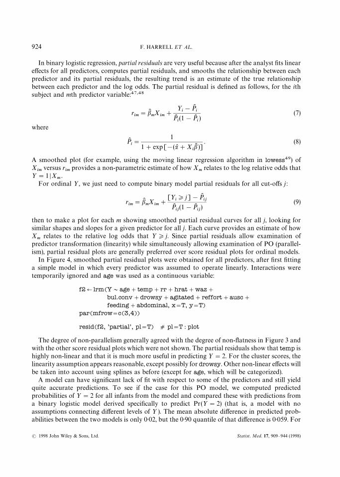
In Figure 4, smoothed partial residual plots were obtained for all predictors, after first fittinga simple model in which every predictor was assumed to operate linearly. Interactions weretemporarily ignored and age was used as a continuous variable:

f2Qlrm(Y&age#temp#rr#hrat#waz#bul.conv#drowsy#agitated#reffort#ausc#feeding#abdominal, x"T, y"T)

par(mfrow"c(3,4))

resid(f2, ’partial’, pl"T) d pl"T : plot

The degree of non-parallelism generally agreed with the degree of non-flatness in Figure 3 andwith the other score residual plots which were not shown. The partial residuals show that temp ishighly non-linear and that it is much more useful in predicting ½"2. For the cluster scores, thelinearity assumption appears reasonable, except possibly for drowsy. Other non-linear effects willbe taken into account using splines as before (except for age, which will be categorized).

A model can have significant lack of fit with respect to some of the predictors and still yieldquite accurate predictions. To see if the case for this PO model, we computed predictedprobabilities of ½"2 for all infants from the model and compared these with predictions froma binary logistic model derived specifically to predict Pr(½"2) (that is, a model with noassumptions connecting different levels of ½ ). The mean absolute difference in predicted prob-abilities between the two models is only 0)02, but the 0)90 quantile of that difference is 0)059. For



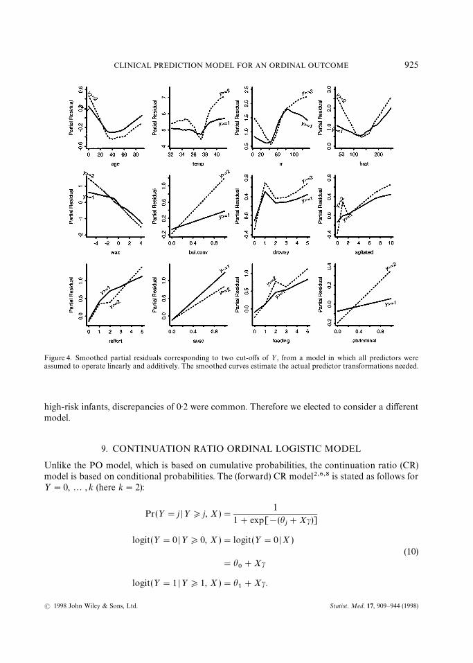
Figure 4. Smoothed partial residuals corresponding to two cut-offs of ½, from a model in which all predictors wereassumed to operate linearly and additively. The smoothed curves estimate the actual predictor transformations needed.

high-risk infants, discrepancies of 0)2 were common. Therefore we elected to consider a differentmodel.

9. CONTINUATION RATIO ORDINAL LOGISTIC MODEL

Unlike the PO model, which is based on cumulative probabilities, the continuation ratio (CR)model is based on conditional probabilities. The (forward) CR model2,6,8 is stated as follows for½"0,2 , k (here k"2):

Pr(½"j D½*j, X)"1

1#exp[!(hj#Xc)]

logit(½"0 D½*0, X )"logit(½"0 DX )(10)

"h0#Xc

logit(½"1 D½*1, X )"h1#Xc.



The CR model has been said to be likely to fit ordinal responses when subjects have to ‘passthrough’ one category to get to the next (which is the case here with respect to SaO

2). The CR

model is a discrete version of the Cox proportional hazards model.To check CR model assumptions, binary logistic model partial residuals are again valuable. We

fit a sequence of binary logistic models using a series of binary events and the correspondingapplicable (increasingly small) subsets of subjects, and plot smoothed partial residuals againstX for all of the binary events. In S-plus we now fit the sequence of binary fits and then use theplot.lrm.partial function, which assembles partial residuals for a sequence of fits and constructsone graph per predictor:

cr0Qlrm(Y""0&age#temp#rr#hrat#waz#bul.conv#drowsy#agitated#reffort#ausc#feeding#abdominal, x"T, y"T)

d Use the update function to save repeating model right hand sided An indicator variable for Y"1 is the response variable belowcrlQupdate(cr0, Y""1&., subset"Y'"1)plot.lrm.partial(cr0, cr1, center"T)

The output is in Figure 5. There is not much more parallelism here than in Figure 4. For the twomost important predictors, ausc and rr, there are strongly differing effects for the differing eventsbeing predicted (for example, ½"0 vs. ½"1 D½*1). As is often the case, there is no oneconstant b model that satisfies assumptions with respect to all predictors simultaneously,especially when there is evidence for non-ordinality for ausc in Figure 2. The CR model will needto be generalized to adequately fit this data set.

10. EXTENDED CONTINUATION RATIO MODEL

By comparing Figures 4 and 5 it is seen that the CR model in its ordinary form has no advantageover the PO model for this data set. The PO model has been extended by Peterson and Harrell15to allow for unequal slopes for some or all of the X’s for some or all levels of ½. This partial POmodel requires specialized software, and with the demise of SAS Version 5 PROC LOGIST,software is not currently available. Armstrong and Sloan6 and Berridge and Whitehead8 showedhow the CR model can be fitted using ordinary binary logistic model software, after certain rowsof the X matrix are duplicated and a new binary ½ vector is constructed. For each subject, oneconstructs separate records by considering successive conditions ½*0, ½*1,2 ,½*k!1for a response variable with values 0, 1,2 , k. The binary response for each applicable conditionor ‘cohort’ is set to 1 if the subject failed at the current ‘cohort’ or ‘risk set’, that is, if ½"j wherethe cohort being considered is ½*j. The constructed cohort variable is carried along with thenew X and ½. This variable is considered to be categorical and its coefficients are fitted by addingk!1 dummy variables to the binary logistic model. The CR model is restated as follows:

Pr(½"j D½*j, X )"1

1#exp[!(a#hj#Xc)]

. (11)

Here a is an overall intercept, h0,0, and h

1,2 , h

k~1are increments from a. In S-plus notation,

the model isy&cohort#X1#X2#X3#2 ,



Figure 5. lowess smoothed partial residual plots for binary models which are components of an ordinal continuationratio model

with cohort denoting a polytomous variable and the columns of X denoted by X1,X22 , etc.The CR model can be extended to allow for some or all of the c’s to change with the cohort or½-cut-off.6 Suppose that non-constant slope is allowed for X1 and X2. The S-plus notation forthe extended model would be

y&cohort*(X1#X2)#X3

The interaction notation (* ) implies that lower-order effects are also included in the model. Theextended CR model is a discrete version of the Cox survival model with time-dependentcovariables.

The cr.setup function in Design returns a list of vectors useful in constructing a data set usedto ‘trick’ a binary logistic function into fitting CR models. The subs vector in this list containsobservation numbers in the original data, some of which are repeated so that subscripting onsubs will cause the subject’s row of predictor variable values to be replicated the desired numberof times (min(½#1, k) times if ½"0, 1,2 , k). Each replication corresponds to the conditioningevent or risk set (cohort) ½*j, and the new dummy response variable y indicates whether or not½"j.



uQcr.setup(Y) d Y is original ordinal response vectorattach(mydata[u$subs,]) d my data is the original dataset

d mydata[i,] subscripts the input data,d using duplicate values of i for repeats

y Qu$y d constructed binary responsecohort Qu$cohort d cohort or risk set categories

Here the cohort variable has values ‘all’, ‘Y'"1’ corresponding to the conditioning events inequation (10). After the attach command runs, vectors such as age are lengthened (to 5553records) by duplicating the correct observations according to the magnitude of a subject’s½ value. Now we fit a fully extended CR model which makes no equal slopes assumptions, that is,the model has to fit ½ assuming the covariables are linear and additive. At this point, we omithrat but add back all variables which were deleted by examining their association with ½. Recallthat most of these 7 cluster scores were summarized using PC

1. Adding back ‘insignificant’

variables will allow us to validate the model fairly using the bootstrap, as well as to obtainconfidence intervals which are not falsely narrow.50

fullQlrm(y&cohort*(ageg*(rcs(temp,5)#rcs(rr,5))#rcs(waz,4)#bul.conv#drowsy#agitated#reffort#ausc#feeding#abdominal#hydration#hxprob#pustular#crying#fever.ill#stop.breath#labor), x"T, y"T)

d x"T, y"T is for pentrace, validate, calibrate belowlatex(anova(full))

This model has LR s2"1824 with 87 d.f. Wald statistics produced by anova(full) are inTable VI. For brevity, tests of non-linear effects and many tests with P'0)1 are not shown.

The global test of the constant slopes assumption in the CR model (test of all interactionsinvolving cohort) has s2"172 with 43 d.f., P(0)0001. Consistent with Figure 5, the formal testsindicate that ausc is the biggest violator, followed by waz and rr.

At this point we select the CR model for this problem because of its flexibility, both in testingthe equal slopes assumption and in parameterizing non-equal-slopes extensions.

11. PENALIZED ESTIMATION

The traditional estimation technique used for logistic models, maximum likelihood estimation(MLE), is optimal (that is, has lowest variance) among techniques which yield unbiased estimatesfor large samples. The bias of an estimator is not its most important attribute, however. Theprobability that a parameter estimate bK

iis close to the true population value is a function of the

mean squared error of that estimate, which is the variance plus the square of the bias. In manycases, especially for small samples, one can sacrifice the bias and lower the variance by a sufficientamount so that the mean squared error of the estimate is lower than that of the MLE. As anexample, if one were using patients’ sex to predict mortality and there were two males in thesample, the probability of death for males would be more reliably estimated by ‘shrinking’ ittoward the probability of death for the overall sample, which is dominated by females. Shrinkagecan be much more general, for example, shrinking a non-linear regression effect toward a lineareffect if the evidence for non-linearity is weak.



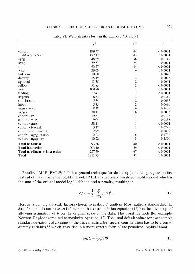
Table VI. Wald statistics for y in the extended CR model

s2 d.f. P

cohort 199)47 44 (0)0001All interactions 172)12 43 (0)0001

ageg 48)89 36 0)0742temp 59)37 24 0)0001rr 93)77 24 (0)0001waz 39)69 6 (0)0001bul.conv 10)80 2 0)0045drowsy 15)19 2 0)0005agitated 13)55 2 0)0011reffort 51)85 2 (0)0001ausc 109)80 2 (0)0001feeding 27)47 2 (0)0001hxprob 6)62 2 0)0364stop.breath 5.34 2 0)0693labor 5)35 2 0)0690ageg]temp 8)18 16 0)9432ageg]rr 38)11 16 0)0015cohort]rr 19)67 12 0)0736cohort]waz 9)04 3 0)0288cohort]ausc 38)11 1 (0)0001cohort]fever.ill 3)17 1 0)0749cohort]stop.breath 2)99 1 0)0839cohort]ageg]temp 2)22 8 0)9736cohort]ageg]rr 10)22 8 0)2500

Total non-linear 93)36 40 (0)0001Total interaction 203)10 59 (0)0001Total non-linear#interaction 257)70 67 (0)0001Total 1211)73 87 (0)0001

Penalized MLE (PMLE)51~53 is a general technique for shrinking (stabilizing) regression fits.Instead of maximizing the log-likelihood, PMLE maximizes a penalized log-likelihood which isthe sum of the ordinal model log-likelihood and a penalty, resulting in

log¸!

1

2j

p+i/1

(sibi)2. (12)

Here s1, s

2,2 , s

pare scale factors chosen to make s

ibiunitless. Most authors standardize the

data first and do not have scale factors in the equation,51 but equation (12) has the advantage ofallowing estimation of b on the original scale of the data. The usual methods (for example,Newton—Raphson) are used to maximize equation (12). The usual default values for s are samplestandard deviations of columns of the design matrix, but special consideration has to be given todummy variables,52 which gives rise to a more general form of the penalized log-likelihood

log¸!

1

2jb@Pb (13)



where P is a penalty matrix. Rows and columns of P can easily be set to zero for parameters forwhich no shrinkage is desired.52,53

The main problem in using PMLE is the choice of j. Many authors use cross-validation tosolve for the j which optimizes an unbiased estimate of predictive accuracy, but it is easy to showthat one must use a huge number of data splits to get a precise estimate of the optimum j. A fasterand usually more reliable strategy, based on findings from a small number of simulation studies, isto choose the j which maximizes the ‘effective’ AIC. Gray (Eq. 2)9)53 and others show how tocompute the ‘effective d.f.’ in this situation (that is, higher j causes more shrinkage which lowersthe effective d.f.). The effective AIC is

LR s2!2]effective d.f. (14)

where LR s2 is the likelihood ratio s2 for the penalized model, but ignoring the penalty function.The lrm function will do PMLE, and a separate function called pentrace searches for the

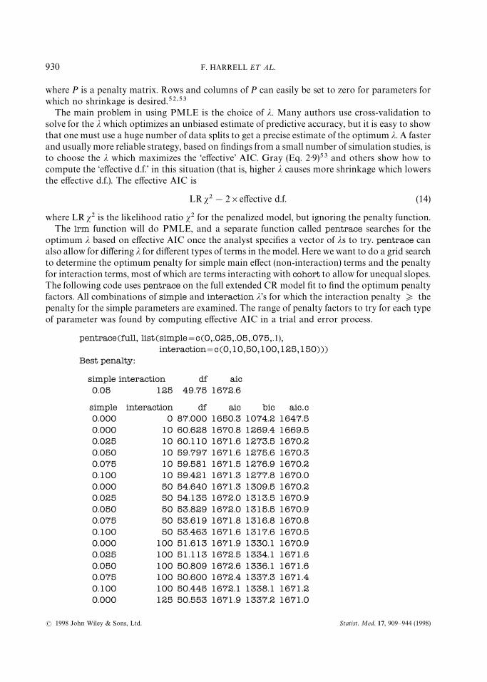
optimum j based on effective AIC once the analyst specifies a vector of js to try. pentrace canalso allow for differing j for different types of terms in the model. Here we want to do a grid searchto determine the optimum penalty for simple main effect (non-interaction) terms and the penaltyfor interaction terms, most of which are terms interacting with cohort to allow for unequal slopes.The following code uses pentrace on the full extended CR model fit to find the optimum penaltyfactors. All combinations of simple and interaction j’s for which the interaction penalty * thepenalty for the simple parameters are examined. The range of penalty factors to try for each typeof parameter was found by computing effective AIC in a trial and error process.

pentrace(full, list(simple"c(0,.025,.05,.075,.1),interaction"c(0,10,50,100,125,150)))

Best penalty:

simple interaction df aic0.05 125 49.75 1672.6

simple interaction df aic bic aic.c0.000 0 87.000 1650.3 1074.2 1647.50.000 10 60.628 1670.8 1269.4 1669.50.025 10 60.110 1671.6 1273.5 1670.20.050 10 59.797 1671.6 1275.6 1670.30.075 10 59.581 1671.5 1276.9 1670.20.100 10 59.421 1671.3 1277.8 1670.00.000 50 54.640 1671.3 1309.5 1670.20.025 50 54.135 1672.0 1313.5 1670.90.050 50 53.829 1672.0 1315.5 1670.90.075 50 53.619 1671.8 1316.8 1670.80.100 50 53.463 1671.6 1317.6 1670.50.000 100 51.613 1671.9 1330.1 1670.90.025 100 51.113 1672.5 1334.1 1671.60.050 100 50.809 1672.6 1336.1 1671.60.075 100 50.600 1672.4 1337.3 1671.40.100 100 50.445 1672.1 1338.1 1671.20.000 125 50.553 1671.9 1337.2 1671.0



*See Hurvich and Tsai54 for the definition of aic.c, the ‘corrected AIC’. Regarding the Bayesian information criterion(bic) of Schwarz,55 several simulations have shown that models selected by BIC had too much shrinkage and hence invalidation samples predicted less well than ones selected using AIC

0.025 125 50.054 1672.6 1341.1 1671.70.050 125 49.750 1672.6 1343.2 1671.70.075 125 49.542 1672.4 1344.4 1671.50.100 125 49.387 1672.1 1345.1 1671.30.000 150 49.653 1671.8 1343.0 1670.90.025 150 49.155 1672.5 1347.0 1671.60.050 150 48.852 1672.5 1349.0 1671.60.075 150 48.643 1672.3 1350.2 1671.50.100 150 48.489 1672.1 1351.0 1671.2

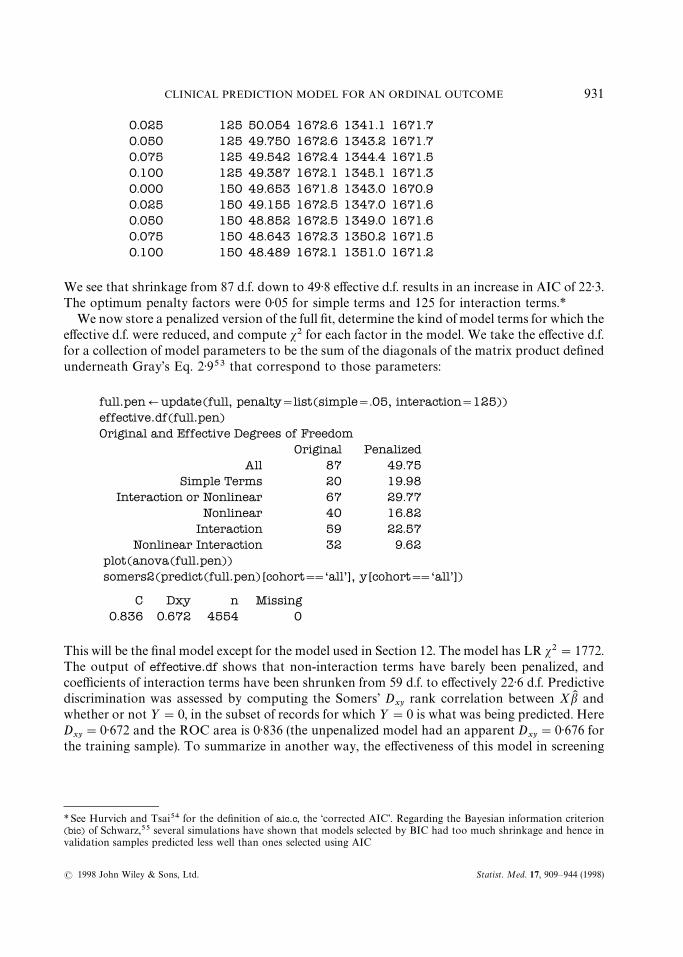
We see that shrinkage from 87 d.f. down to 49)8 effective d.f. results in an increase in AIC of 22)3.The optimum penalty factors were 0)05 for simple terms and 125 for interaction terms.*

We now store a penalized version of the full fit, determine the kind of model terms for which theeffective d.f. were reduced, and compute s2 for each factor in the model. We take the effective d.f.for a collection of model parameters to be the sum of the diagonals of the matrix product definedunderneath Gray’s Eq. 2)953 that correspond to those parameters:

full.penQupdate(full, penalty"list(simple".05, interaction"125))effective.df(full.pen)Original and Effective Degrees of Freedom

Original PenalizedAll 87 49.75

Simple Terms 20 19.98Interaction or Nonlinear 67 29.77

Nonlinear 40 16.82Interaction 59 22.57

Nonlinear Interaction 32 9.62plot(anova(full.pen))somers2(predict(full.pen)[cohort""‘all’], y[cohort""‘all’])

C Dxy n Missing0.836 0.672 4554 0

This will be the final model except for the model used in Section 12. The model has LR s2"1772.The output of effective.df shows that non-interaction terms have barely been penalized, andcoefficients of interaction terms have been shrunken from 59 d.f. to effectively 22)6 d.f. Predictivediscrimination was assessed by computing the Somers’ D

xyrank correlation between XbK and

whether or not ½"0, in the subset of records for which ½"0 is what was being predicted. HereD

xy"0)672 and the ROC area is 0)836 (the unpenalized model had an apparent D

xy"0)676 for

the training sample). To summarize in another way, the effectiveness of this model in screening



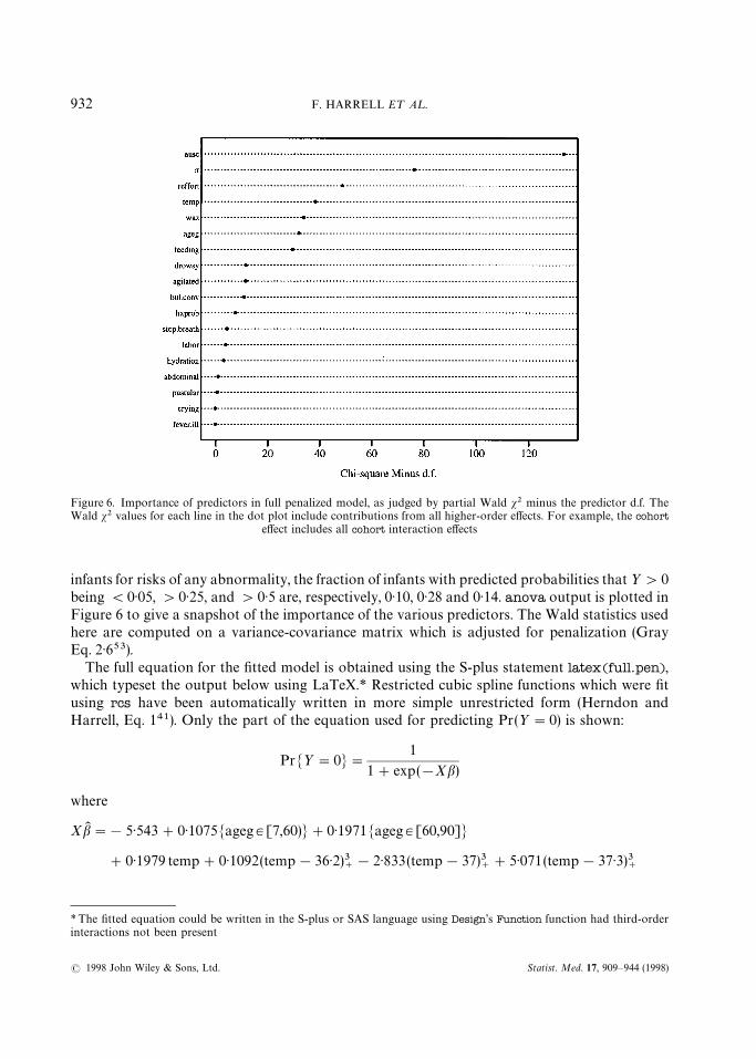
Figure 6. Importance of predictors in full penalized model, as judged by partial Wald s2 minus the predictor d.f. TheWald s2 values for each line in the dot plot include contributions from all higher-order effects. For example, the cohort

effect includes all cohort interaction effects

*The fitted equation could be written in the S-plus or SAS language using Design’s Function function had third-orderinteractions not been present

infants for risks of any abnormality, the fraction of infants with predicted probabilities that ½'0being (0)05, '0)25, and '0)5 are, respectively, 0)10, 0)28 and 0)14. anova output is plotted inFigure 6 to give a snapshot of the importance of the various predictors. The Wald statistics usedhere are computed on a variance-covariance matrix which is adjusted for penalization (GrayEq. 2)653).

The full equation for the fitted model is obtained using the S-plus statement latex(full.pen),which typeset the output below using LaTeX.* Restricted cubic spline functions which were fitusing rcs have been automatically written in more simple unrestricted form (Herndon andHarrell, Eq. 141). Only the part of the equation used for predicting Pr(½"0) is shown:

PrM½"0N"1

1#exp(!Xb)

where

XbK "!5)543#0)1075Mageg3[7,60)N#0)1971Mageg3[60,90]N

#0)1979 temp#0)1092(temp!36)2)3`!2)833(temp!37)3

`#5)071(temp!37)3)3

`



!2)508(temp!37)7)3`#0)1606(temp!39)3

`

#0)02091 rr!6)337]10~5(rr!32)3`#8)405]10~5(rr!42)3

`#6)152]10~5(rr!49)3

`

!0)0001018(rr!59)3`#1)96]10~5(rr!76)3

`

!0)0759waz#0)02509(waz#2)9)3`!0)1185(waz#0)75)3

`#0)1226(waz!0)28)3

`

!0)02916(waz!1)73)3`!0)4418bul.conv!0)08185drowsy!0)05327 agitated

!0)2304 reffort!1)159 ausc!0)16 feeding!0)1609 abdominal

!0)0541hydration#0)08086hxprob#0)00752pustular#0)04712 crying

#0)004299 fever.ill!0)3519 stop.breath#0)06864 labor

#Mageg3[7,60)N[6)5]10~5 temp!0)0028(temp!36)2)3`!0)008691(temp!37)3

`

!0)004988(temp!37)3)3`#0)02592(temp!37)7)3

`!0)009445(temp!39)3

`]

#Mageg3[60,90]N[0)000132temp!0)001826(temp!36)2)3`!0)0164(temp!37)3

`

!0)0476(temp!37)3)3`#0)09142(temp!37)7)3

`!0)02559(temp!39)3

`]

#Mageg3[7,60)N[!0)0009438 rr!1)045]10~6(rr!32)3`!1)67]10~6(rr!42)3

`

!5)189]10~6[rr!49)3`#1)429]10~5(rr!59)3

`!6)382]10~6(rr!76)3

`]

#Mageg3[60,90]N[!0)001921 rr!5)521]10~6(rr!32)3`!8)628]10~6(rr!42)3

`

!4)147]10~6(rr!49)3`#3)813]10~5(rr!59)3

`!1)984]10~5(rr!76)3

`]

and McN"1 if subject is in group c, otherwise, (x)`"x if x'0, 0 otherwise.

To show the shapes of effects of the predictors we use the following code. For the continuousvariables temp and rr which interact with age group, we show the effects for all three age groups,separately for each ½ cut-off. All effects have been centred so that the log odds at the medianpredictor value is zero when cohort"‘all’, so these plots actually show log odds relative to thereference values. The patterns in Figure 7 are in agreement with those in Figure 5:

par(mfrow"c(4,4))ylQc(!2.5, 1) d put all plots on common y-axis scale

d Plot predictors which interact with another predictord Vary ageg over all age groups, then vary temp over itsd default range (10th smallest to 10th largest values in data)d Make a separate plot for each ‘cohort’d ref.zero centers effects using median x

for(co in levels(cohort)) Mplot(full.pen, temp"NA, ageg"NA, cohort"co, ref.zero"T, ylim"yl, conf.int"F)text(37.5, 1.5, co) d add title showing current cohort

N



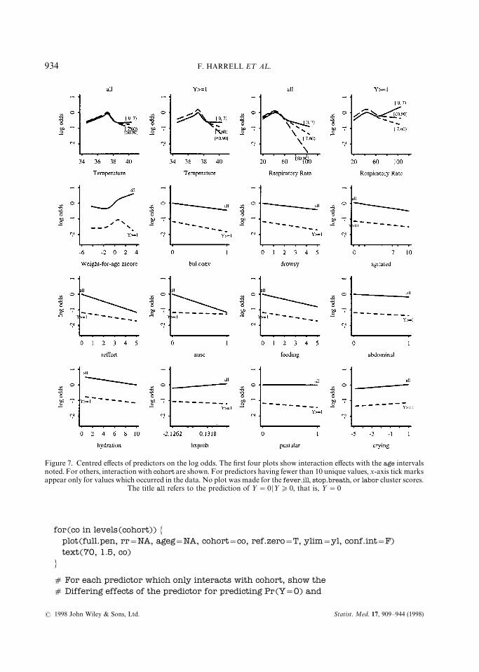
Figure 7. Centred effects of predictors on the log odds. The first four plots show interaction effects with the age intervalsnoted. For others, interaction with cohort are shown. For predictors having fewer than 10 unique values, x-axis tick marksappear only for values which occurred in the data. No plot was made for the fever.ill, stop.breath, or labor cluster scores.

The title all refers to the prediction of ½"0 D½*0, that is, ½"0

for(co in levels(cohort)) Mplot(full.pen, rr"NA, ageg"NA, cohort"co, ref.zero"T, ylim"yl, conf.int"F)text(70, 1.5, co)

N

d For each predictor which only interacts with cohort, show thed Differing effects of the predictor for predicting Pr(Y"0) and



*The lasso method of Tibshirani57 addresses this problem

d Pr(Y"1 DY'0) on the same graph

plot(full.pen, waz "NA, cohort"NA, ref.zero"T, ylim"yl, conf.int"F)plot(full.pen, bul.conv"NA, cohort"NA, ref.zero"T, ylim"yl, conf.int"F)) ) ) )

plot(full.pen, crying "NA, cohort"NA, ref.zero"T, ylim"yl, conf.int"F)

12. USING APPROXIMATIONS TO SIMPLIFY THE MODEL

It is tempting to use P-values and stepwise methods to develop a parsimonious prediction model.Besides invalidating confidence limits and causing measures of predictive accuracy such asadjusted R2 to be optimistic, there are many other reasons not to rely on stepwise techniques (seeHarrell et al.20 for citations). We follow Spiegelhalter’s advice to use full model fits in conjunctionwith shrinkage.56

Parsimonious models can be developed, however, by approximating predictions from themodel to any desired level of accuracy. Let K "Xb denote the predicted log odds from the fullpenalized ordinal model, including multiple records for subjects with ½'0. Then we can usea variety of techniques to approximate K from a subset of the predictors (in their raw form). Withthis approach one can immediately see what is lost over the full model by computing, for example,the mean absolute error in predicting K . Another advantage to full model approximations is thatshrinkage used in computing K is inherited by any model that predicts K . In contrast, the usualstepwise methods result in bK that are too large since the final coefficients are estimated as if themodel structure was prespecified.*

Even though CART (classification and regression trees58) when used on X and ½ often findsprediction rules that validate poorly because of the extremely large number of models searched,27CART can be very useful as an approximator for a complex model. For the current problem,CART would be particularly useful as it would result in a prediction tree that would be easy forhealth workers to use. Unfortunately, a 50-node CART was required to predict K with anR2*0)9, and the mean absolute error in the predicted logit was still 0)4. This will happen whenthe model contains many important continuous variables.

We chose to approximate the full model using its important components, by using a stepdowntechnique predicting K from all of the component variables using ordinary least squares. In usingstepdown with the least squares function ols in Design there is a problem with infinite F statisticswhen the initial R2"1)0, so we will specify p"1 to ols. Because cohort interacts with thepredictors, separate approximations can be developed for each level of ½. For this example weapproximate the log odds that ½"0 using the cohort of patients used for determining ½"0,that is, ½*0 or cohort"‘all’:

plogit Qpredict(full.pen)

fQols(plogit&ageg*(rcs(temp,5)#rcs(rr,5))#rcs(waz,4)#bul.conv#drowsy#agitated#reffort#ausc#feeding#



*To see how this compares with prediction using the full model, the extra clinical signs in that model that are not in theapproximate model were predicted individually on the basis of XbK from the reduced model along with the signs that are inthat model, using ordinary linear regression. The signs not specified when evaluating the approximate model were then setto predicted values based on the values given for the 6-day old infant above. The resulting XbK for the full model is !0)81and the predicted probability is 0)31, as compared with !0)68 and 0)34 quoted above

abdominal#hydration#hxprob#pustular#crying#fever.ill#stop.breath#labor, sigma"1,subset"cohort"‘all’)

d Do fast backward stepdownfastbw(f, aics"1e10) d 1e10 causes all variables to eventually be

d deleted so can see most important ones in order

d Fit an approximation to the full penalized model using mostd important variablesfull.approxQols(plogit&rcs(temp,5)#ageg*rcs(rr,5)#rcs(waz,4)#

bul.conv#drowsy#reffort#ausc#feeding,subset"cohort""‘all’)

The approximate model had R2 against the full penalized model of 0)972, and the mean absoluteerror in predicting K was 0)17. The D

xyrank correlation between the approximate model’s

predicted logit and the binary event ½"0 is 0)665 as compared with the full model’s Dxy"0)672.

Next, turn to diagramming this model approximation so that all predicted values can becomputed without the use of a computer. We draw a type of nomogram which converts eacheffect in the model to a 0—100 scale which is just proportional to the log odds. These points areadded across predictors to derive the ‘total points’, which are converted to K and then topredicted probabilities. For the interaction between rr and ageg, Design’s nomogram functionautomatically constructs 3 rr axes — only one is added into the total point score for a givensubject. Here we draw a nomogram for predicting the probability that ½'0, which is1!Pr(½"0). This probability is derived by negating bK and XbK in the model derived to predictPr(½"0).

fQfull.approxf$coefficients Qf$coefficientsf$linear-predictors Qf$linear.predictors

nomogram(f,temp"32:41, rr"seq(20,120,by"10), waz"seq(!1.5,2,by".5),fun"plogis, funlabel"’Pr(Y'0)’,fun.at"c(.02,.05,seq(.1,.9,by".1),.95,.98))

d plogis is S-PLUS’s builtin 1/(1#exp(!x)) function

The nomogram is shown in Figure 8. As an example in using the nomogram, a 6-day old infantgets approximately 9 points for having a respiratory rate of 30/min, 19 points for havinga temperature of 39°C, 11 points for waz"0, 14 points for drowsy"5, and 15 points forreffort"2. Assuming that bull.conv"ausc"feeding"0, that infant gets 68 total points. Thiscorresponds to XbK "!0)6 and a probability of 0)35. Values computed directly from thefull.approx formula were XbK "!0)68 and a probability of 0)34.*



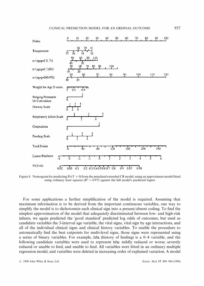
Figure 8. Nomogram for predicting Pr(½'0) from the penalized extended CR model, using an approximate model fittedusing ordinary least squares (R2"0)972 against the full model’s predicted logits)

For some applications a further simplification of the model is required. Assuming thatmaximum information is to be derived from the important continuous variables, one way tosimplify the model is to dichotomize each clinical sign into a present/absent coding. To find thesimplest approximation of the model that adequately discriminated between low- and high-riskinfants, we again predicted the ‘good standard’ predicted log odds of outcomes, but used ascandidate variables the 3-interval age variable, the vital signs, vital sign by age interactions, andall of the individual clinical signs and clinical history variables. To enable the procedure toautomatically find the best cutpoints for multi-level signs, those signs were represented usinga series of binary variables. For example, hfa (history of feeding) is a 0—4 variable, and thefollowing candidate variables were used to represent hfa: mildly reduced or worse; severelyreduced or unable to feed, and unable to feed. All variables were fitted in an ordinary multipleregression model, and variables were deleted in increasing order of explained variation. A model



which retained 7 individual signs resulting in Dxy"0)664 and R2 against the optimal model’s

predicted logit of 0)954.

13. VALIDATING THE MODEL

Most analysts validate a fitted model using held-back data, but this method has severe draw-backs.20 The bootstrap technique59 allows the analyst to derive bias (overfitting) — correctedestimates of predictive accuracy without holding back valuable data during the model develop-ment phase. The steps required for using the bootstrap to bias-correct indexes such as D

xyand

calibration error was summarized in Harrell et al.20 For the full CR model which was fitted usingPMLE, we used 150 bootstrap replications to estimate and then to correct for optimism invarious statistical indexes: D

xy; generalized R2;60 intercept and slope of a linear recalibration

equation for XbK (related to Section 7 of van Houwelingen and le Cessie;61 see also Phillipset al.62); the maximum calibration error for Pr(½"0) based on the linear-logistic recalibration(Emax), and the Brier quadratic probability score B.63 PMLE is used at each of the 150resamples. During the bootstrap simulations, we sample with replacement from the patients andnot from the 5553 expanded records, hence the specification cluster"u$subs, where u$subs isthe vector of sequential patient numbers computed from cr.setup above. To be able to measurethe predictive accuracy of the predicted probability of a single event, the subset parameter isspecified so that Pr(½"0) is being assessed even though 5553 observations are used to developeach of the 150 models. The output and the S-plus statement used to obtain the output are shownbelow:

validate(full.pen, B"150, cluster"u$subs, subset"cohort""‘all’)

index.orig training test optimism index.corrected nDxy 0.672 0.675 0.666 0.009 0.662 150R2 0.376 0.383 0.370 0.013 0.363 150

Intercept !0.031 !0.033 0.001 !0.034 0.003 150Slope 1.029 1.031 1.002 0.029 1.000 150Emax 0.000 0.000 0.001 0.001 0.001 150

B 0.120 0.119 0.121 !0.002 0.122 150

We see that for the apparent Dxy"0)672 the optimism from overfitting was estimated to be 0)009

for the PMLE model, so the bias-corrected estimate of predictive discrimination is 0)662. Theintercept and slope needed to recalibrate XbK to a 45° line are very near (0, 1). The estimate of themaximum calibration error in predicting Pr(½"0) is 0)001 which is quite satisfactory. Thecorrected Brier score is 0)122.

The simple calibration statistics just listed do not address the issue of whether predicted valuesfrom the model are miscalibrated in a non-linear way. Steps for estimating bias-correctedcalibration curves for survival time models and for non-parametrically estimating a smoothcalibration curve for a binary logistic model on a separate validation sample were givenpreviously.20 Putting these two techniques together we arrive at the following plan for esti-mating a calibration curve using the bootstrap, with the only assumption being the smoothness ofthe curve. Choose a single binary event for which to check the calibration of the estimated



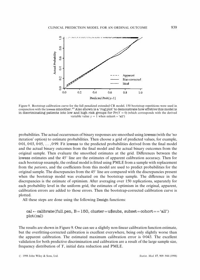
Figure 9. Bootstrap calibration curve for the full penalized extended CR model. 150 bootstrap repetitions were used inconjunction with the lowess smoother.49 Also shown is a ‘rug plot’ to demonstrate how effetive this model isin discriminating patients into low and high risk groups for Pr(½"0) (which corresponds with the derived

variable value y"1 when cohort"’all’)

probabilities. The actual occurrences of binary responses are smoothed using lowess (with the ‘noiteration’ option) to estimate probabilities. Then choose a grid of predicted values, for example,0)01, 0)03, 0)05,2 , 0)99. Fit lowess to the predicted probabilities derived from the final modeland the actual binary outcomes from the final model and the actual binary outcomes from theoriginal sample. Then evaluate the smoothed estimates at the grid. Differences between thelowess estimates and the 45° line are the estimates of apparent calibration accuracy. Then foreach bootstrap resample, the ordinal model is fitted using PMLE from a sample with replacementfrom the patients, and the coefficients from this model are used to predict probabilities for theoriginal sample. The discrepancies from the 45° line are compared with the discrepancies presentwhen the bootstrap model was evaluated on the bootstrap sample. The difference in thediscrepancies is the estimate of optimism. After averaging over 150 replications, separately foreach probability level in the uniform grid, the estimates of optimism in the original, apparent,calibration errors are added to those errors. Then the bootstrap-corrected calibration curve isplotted.

All these steps are done using the following Design functions:

calQcalibrate(full.pen, B"150, cluster"u$subs, subset"cohort""‘all’)plot(cal)

The results are shown in Figure 9. One can see a slightly non-linear calibration function estimate,but the overfitting-corrected calibration is excellent everywhere, being only slightly worse thanthe apparent calibration. The estimated maximum calibration error is 0)043. The excellentvalidation for both predictive discrimination and calibration are a result of the large sample size,frequency distribution of ½, initial data reduction and PMLE.



14. SUMMARY

Clinically-guided variable clustering and item weighting, done with very limited use of theoutcome variable, resulted in a great reduction in the number of candidate predictor degrees offreedom and hence increased the true predictive accuracy of the model. Sources summarizingclusters of clinical signs, along with the temperature, respiratory rate, and weight-for-age aftersuitable non-linear transformation and allowance for interactions with age, are powerful pre-dictors of the ordinal response. Graphical methods are effective for detecting lack of fit in the POand CR models and for diagramming the final model. Model approximation is a better approachthan stepwise methods (that use ½) to develop parsimonious clinical prediction tools. Approxim-ate models inherit the shrinkage from the full model. For the ordinal model developed here,substantial shrinkage of the full model was needed.

The bootstrap, as in a wide variety of other situations, is an effective tool for validating anordinal logistic model with respect to discrimination and calibration without having the need tohold back data during model development. The final CR ordinal logistic model accuratelypredicted severity of diagnosis/outcome (as summarized by several disparate outcome variables)in infants screened for pneumonia, sepsis, and meningitis in developing countries. There wasnothihg about the continuation ratio model that made it fit the data set better than other ordinalmodels (which we have found to be the case in one other large data set), and in fact there is someevidence that the equal-slopes CR model fits the data more poorly than the equal-slopes POmodel. The real benefit of the CR model is that using standard binary logistic model software onecan flexibly specify how the equal-slopes assumption can be relaxed.

Faraway64 has demonstrated how all data-driven steps of the modelling process increase thereal variance in ‘final’ parameter estimates, when one estimates variances without assuming thatthe final model was prespecified. For ordinal regression modelling, the most important modellingsteps are (i) choice of predictor variables; (ii) selecting or modelling predictor transformations; and(iii) allowance for unequal slopes across ½-cut-offs (that is, non-PO or non-CR). Regarding steps(ii) and (iii) one is tempted to rely on graphical methods such as residual plots to make detours inthe strategy, but it is very difficult to estimate variances or to properly penalize assessments ofpredictive accuracy for subjective modelling decisions. Regarding (i), shrinkage has been provento work better than stepwise variable selection when one is attempting to build a main-effectsmodel.56 Choosing a shrinkage factor is a well-defined, smooth, and often a unique process asopposed to binary decisions on whether variables are ‘in’ or ‘out’ of the model. Likewise, insteadof using arbitrary subjective (residual plots) or objective (s2 due to cohort]covariable interac-tions, that is, non-constant covariable effects) assessments, shrinkage can systematically allowmodel enhancements in so far as the information content in the data will support, through the useof differential penalization. Shrinkage is a solution to the dilemma faced when the analystattempts to choose between a parsimonious model and a more complex one that fits the data.Penalization does not require the analyst to make a binary decision, and it is a process that can bevalidated using the bootstrap.



APPENDIX

WHO/ARI Young Infant Multicentre Study Group*

Study sites Addis Ababa,Ethiopia

Fajara, Gambia Goroka, PapuaNew Guinea

Manila, Philippines

Principalinvestigator

Lulu Muhe Kim Mulholland Deborah Lehmann Salvacion Gatchalian

Co-investigators, Olayinka Ogunlesi Gerard Saleu Beatriz QuiambaoStudy coordinators Martin Weber

Other investigators,clinicians

Meaza Tilahun Mark Manary Alphonse Rongap Ana Marie MorelesSileshi Lulseged Ayo Palmer Mexy Kakazo Leticia AbrahamSenait Kebede Pioto Namuigi

Sebeya LupiwaRebecca sehuko

Bacteriologists Afeworti Yohaness Richard Adegbola Alison Clegg Lydia SombreroBahrie Belete Osman Secka Audrey Michael Ma. Victoria AbrahamSigne Ringertz Tony Lupiwa

Matthew OmenaMark Mens

Radiologists Tsegaye Desta

Data management KidanemariamWlyesus

Joseph Bangali Don Lewis Elinor S. SunicoTeresita C. Cedulla

Institution/hospitals

Department ofPaediatrics and ChildHeath, Ethio-SwedishChildren’s Hospital,Addis AbabaUniversity

Medical ResearchCouncil Hospital andRoyal VictoriaHospital

Papua New GuineaInstitute of MedicalResearch Goroka BaseHospital

Research Institute ofTropical TropicalMedicine, PhillippinesGeneral Hospital,Quezon City GeneralHospital

Institution DirectorsNebiat Tafari Brian Greenwood Michael P. Alpers

*Not inclusivesDeceased

Study Co-ordination

Scientific co-ordinator: Dr Sandy Gove, WHO/ARIData management: Dr Peter Byass, University of Nottingham Medical SchoolData analysis: Dr Frank Harrell, University of Virginia, Charlottesville Mrs Karen Mason, WHO/ARIManagement, logistic, supplies: Mrs Frances McCaul, WHO/ARI

Mrs Sue Parker, WHO/ARIStudy advisors: Dr Claire Broome, Centers for Disease Control (CDC), Atlanta

Dr H. F. Eichenwald, University of Texas Southwestern Medical Center, DallasMr Mike Gratten, Queensland Institute of Medical Research, BrisbaneDr P. Margolis, University of North Carolina at Chapel HillDr R. Facklam, CDC, Atlanta

Radiology working group: Dr H. Tschappeler, Universitat BernDr A. Lamont, The Leicester Royal InfirmaryDr G. M. A. Hendry, Royal Hospital for Sick Children, EdinburghProfessor Philip E. S. Palmer, University of California, Davis

ACKNOWLEDGEMENTS

This work was supported by The World Health Organization ARI Programme, and for F.Harrell, Research Grants HS-06830 and HS-07137 from the Agency for Health Care Policy andResearch, Rockville, Maryland, U.S.A., and grants from the Robert Wood Johnson Foundation,



Princeton, NJ, U.S.A. F. Harrell wishes to dedicate his work on this project to the memory of hisdear colleague L. Richard Smith whose critical reading of this paper resulted in significantimprovements.

REFERENCES

1. Walker, S. H. and Duncan, D. B. ‘Estimation of the probability of an event as a function of severalindependent variables’, Biometrika, 54, 167—178 (1967).

2. Fienberg, S. E. ¹he Analysis of Cross-Classified Data, 2nd edn, MIT Press, Cambridge, MA, 1980.3. Agresti, A. ‘A survey of models for repeated ordered categorical response data’, Statistics in Medicine, 8,

1209—1224 (1989).4. Anderson, J. A. and Philips, P. R. ‘Regression, discrimination and measurement models for ordered

categorical variables’, Applied Statistics, 30, 22—31 (1981).5. Anderson, J. A. ‘Regression and ordered categorical variables’, Journal of the Royal Statistical Society,

Series B, 46, 1—30 (1984).6. Armstrong, B. G. and Sloan, M. ‘Ordinal regression models for epidemiologic data’, American Journal of

Epidemiology, 129, 191—204 (1989).7. Ashby, D., West, C. R. and Ames, D. ‘The ordered logistic regression model in psychiatry: Rising

prevalence of dementia in old people’s homes’, Statistics in Medicine, 8, 1317—1326 (1989).8. Berridge, D. M. and Whitehead, J. ‘Analysis of failure time data with ordinal categories of response’,

Statistics in Medicine, 10, 1703—1710 (1991).9. Brazer, S. R., Pancotto, F. S., Long III, T. T., Harrell, F. E., Lee, K. L., Tyor, M. P. and Pryor, D. B.

‘Using ordinal logistic regression to estimate the likelihood of colorectal neoplasia’, Journal of ClinicalEpidemiology, 44, 1263—1270 (1991).

10. Cox, C. ‘Location-scale cumulative odds models for ordinal data: A generalized non-linear modelapproach’, Statistics in Medicine, 14, 1191—1203 (1995).

11. Greenland, S. ‘Alternative models for ordinal logistic regression’, Statistics in Medicine, 13, 1665—1677(1994).

12. Hastie, T. J., Botha, J. L. and Schnitzler, C. M. ‘Regression with an ordered categorical response’,Statistics in Medicine, 8, 785—794 (1989).

13. Koch, G. G., Amara, I. A. and Singer, J. M. ‘A two-stage procedure for the analysis of ordinal categoricaldata’, in Sen, P. K. (ed.), BIOS¹A¹IS¹ICS: Statistics in Biomedical, Public Health and EnvironmentalSciences, Elsevier Science Publishers B.V., North-Holland, 1985.

14. McCullagh, P. ‘Regression models for ordinal data’, Journal of the Royal Statistical Society, Series B, 42,109—142 (1980).

15. Peterson, B. and Harrell, F. E. ‘Partial proportional odds models for ordinal response variables’, AppliedStatistics, 39, 205—217 (1990).

16. Whitehead, J. ‘Simple size calculations for ordered categorical data’, Statistics in Medicine, 12,2257—2271 (1993).

17. Cole, T. J., Morley, C. J., Thornton, A. J., Fowler, M. A. and Hewson, P. H. ‘A scoring system to quantifyillness in babies under 6 months of age’, Journal of Royal Statistical Society, Series A, 154, 287—304(1991).

18. Yee, T. W. and Wild, C. J. ‘Vector generalized additive models’, Journal of the Royal Statistical Society,Series B, 58, 481—493 (1996).

19. Harrell, F. E., Lee, K. L., Califf, R. M., Pryor, D. B. and Rosati, R. A. ‘Regression modelling strategies forimproved prognostic prediction’, Statistics in Medicine, 3, 143—152 (1984).

20. Harrell, F. E., Lee, K. L. and Mark, D. B. ‘Multivariable prognostic models: issues in developing models,evaluating assumptions and adequacy, and measuring and reducing errors’, Statistics in Medicine, 15,361—387 (1996).

21. MathSoft. S-Plus ºser’s Manual, »ersion 2.3, MathSoft, Inc., Seattle WA, 1995.22. Harrell, F. E. ‘Design: S-Plus functions for biostatistical/epidemiologic modeling, testing, estimation,

validation, graphics, prediction, and typesetting by storing enhanced model design attributes in the fit.UNIX and Microsoft Windows versions available from http://www.med.virginia.edu/medicine/clinical/hes/biostat.htm’ 1997.



23. WHO/ARI Study Group on the Clinical Signs and Etiological agents of Pneumonia, Sepsis andMeningitis in Young Infants, ‘Study methods’, in preparation (1997).

24. Zhou, X. ‘Effect of verification bias on positive and negative predictive values’, Statistics in Medicine, 13,1737—1745 (1994).

25. WHO/ARI Study Group on the Clinical Signs and Etiological Agents of Pneumonia, Sepsis andMeningitis in Young Infants, ‘Ordinal outcome scale’, in preparation (1997).

26. Follmann, D. ‘Multivariate tests for multiple endpoints in clinical trials’, Statistics in Medicine, 14,1163—1175 (1995).

27. Harrell, F. E., Lee, K. L., Matchar, D. B. and Reichert, T. A. ‘Regression models for prognosticprediction: Advantages, problems, and suggested solutions’, Cancer ¹reatment Reports, 69, 1071—1077(1985).

28. Marshall, G., Grover, F. L., Henderson, W. G. and Hammermeister, K. E. ‘Assessment of predictivemodels for binary outcomes: An empirical approach using operative death from cardiac surgery’,Statistics in Medicine, 13, 1501—1511 (1994).

29. D’Agostino, R. B., Belanger, A. J., Markson, E. W., Kelly-Hayes, M. and Wolf, P. A. ‘Development ofhealth risk appraisal functions in the presence of multiple indicators: The Framingham Study nursinghome institutionalization model’, Statistics in Medicine, 14, 1757—1770 (1995).

30. Cureton, E. E. and D’Agostino, R. B. Factor Analysis, An Applied Approach, Erlbaum Publishers, NewJersey, 1983.

31. Sarle, W. S. ‘The VARCLUS procedure’, in SAS/S¹A¹ºser’s Guide, vol. 2, 4th edn, SAS Institute, Inc.,Cary NC, 1990, Chapter 43, pp. 1641—1659.

32. Hoeffding, W. ‘A non-parametric test of independence’, Annals of Mathematical Statistics, 19, 546—557(1948).

33. Venables, W. N. and Ripley, B. D. Modern Applied Statistics with S-Plus, Springer-Verlag, New York,1994.

34. Jolliffe, I. T. Principal Component Analysis, Springer-Verlag, New York, 1986.35. Jackson, J. E. A ºser’s Guide to Principal Components, Wiley, New York, 1991.36. Kuhfeld, W. F., ‘The PRINQUAL procedure’, in SAS/S¹A¹ºser’s Guide, vol. 2, 4th edn, SAS Institute,

Inc., Cary NC, 1990, Chapter 34, pp. 1265—1323.37. Atkinson, A. C. ‘A note on the generalized information criterion for choice of a model’, Biometrika, 67,

413—418 (1980).38. Stone, C. J. and Koo, C. Y. ‘Additive splines in statistics’, Proceedings of the Statistical Computing

Section ASA, 45—48 (1995).39. Devlin, T. F. and Weeks, B. J. ‘Spline functions for logistic regression modeling’, in Proceedings of the

Eleventh Annual SAS ºsers Group International Conference, SAS Institute, Inc., Cary NC, 1986,pp. 646—651.

40. Harrell, F. E., Lee, K. L. and Pollock, B. G. ‘Regression models in clinical studies: Determiningrelationships between predictors and response’, Journal of the National Cancer Institute, 80, 1198—1202(1988).

41. Herndon, J. E. and Harrell, F. E. ‘The restricted cubic spline hazard model’, Communications in Statistics— ¹heory and Methods, 19, 639—663 (1990).

42. Lamport, L. ¸a¹eX: A Document Preparation System, 2nd edn, Addison-Wesley, Reading, MA,1994.

43. SAS Institute, Inc. SAS/S¹A¹ ºser’s Guide, vol. 2, 4th edn, SAS Institute, Inc., Cary NC, 1990.44. Schoenfeld, D. ‘Partial residuals for the proportional hazards regression model’, Biometrika, 69, 239—241

(1982).45. Grambsch, P. and Therneau, T. ‘Proportional hazards tests and diagnostics based on weighted

residuals’, Biometrika, 81, 515—526 (1994). Amendment and corrections in 82, 668 (1995).46. Cox, D. R. ‘Regression models and life-tables (with discussion)’, Journal of the Royal Statistical Society

Series B, 34, 187—220 (1972).47. Landwehr, J. M., Pregibon, D. and Shoemaker, A. C. ‘Graphical methods for assessing logistic

regression models (with discussion)’, Journal of the American Statistical Association, 79, 61—83 (1984).48. Collett, D. Modelling Binary Data, Chapman and Hall, London 1991.49. Cleveland, W. S. ‘Robust locally weighted regression and smoothing scatterplots’, Journal of the

American Statistical Association, 74, 829—836 (1979).



50. Altman, D. G. and Andersen, P. K. ‘Bootstrap investigation of the stability of a Cox regression model’,Statistics in Medicine, 8, 771—783 (1989).

51. le Cessie, S. and van Houwelingen, J. C. ‘Ridge estimators in logistic regression’, Applied Statistics, 41,191—201 (1992).

52. Verweij, P. and van Houiwelingen, H. C. ‘Penalized likelihood in Cox regression’, Statistics in Medicine,13, 2427—2436 (1994).

53. Gray, R. J. ‘Flexible methods for analyzing survival data using splines, with applications to breast cancerprognosis’, Journal of the American Statistical Association, 87, 942—951 (1992).

54. Hurvich, C. M. and Tsai, C. ‘Regression and time series model selection in small samples’, Biometrika,76, 297—307 (1989).

55. Schwarz, G. ‘Estimating the dimension of a model’, Annals of Statistics, 6, 461—464 (1978).56. Spiegelhalter, D. J. ‘Probabilistic prediction in patient management’, Statistics in Medicine, 5, 421—433

(1986).57. Tibshirani, R. ‘Regression shrinkage and selection via the lasso’, Journal of the Royal Statistical Society

Series B, 58, 267—288 (1996).58. Breiman, L., Friedman, J. H., Olshen, R. A. and Stone, C. J., Classification and Regression ¹rees,

Wadsworth and Brooks/Cole Pacific Grove, CA, 1984.59. Efron, B. and Tibshirani, R. An Introduction to the Bootstrap, Chapman and Hall, New York, 1993.60. Nagelkerke, N. J. D. ‘A note on a general definition of the coefficient of determination’, Biometrika, 78,

691—692 (1991).61. van Houwelingen, J. C. and le Cessie, S. ‘Predictive value of statistical models’, Statistics in Medicine, 8,

1303—1325 (1990).62. Phillips, A. N., Thompson, S. G. and Pocock, S. J. ‘Prognostic scores for detecting a high risk group:

Estimating the sensitivity when applied to new data’, Statistics in Medicine, 9, 1189—1198 (1990).63. Brier, G. W. ‘Verification of forecasts expressed in terms of probability’, Monthly ¼eather Review, 75,

1—3 (1950).64. Faraway, J. J. ‘The cost of data analysis’, Journal of Computational and Graphical Statistics, 1, 213—229

(1992).



Documents

TUTORIAL IN BIOSTATISTICS DEVELOPMENT OF A CLINICAL ...lcc.uma.es/~jja/recidiva/064.pdf · and Etiological Agents of Pneumonia, Sepsis and Meningitis in Young Infants FRANK E. HARRELL,