Embed Size (px)
Citation preview

ITC Data Analysis in Origin®
Tutorial GuideVersion 5.0, October 1998
The Calorimetry Experts
Using Origin® scientific plotting software to analyze calorimetric datafrom the MicroCal Omega, MCS or VP-ITC isothermal titration
calorimeters.


Table of Contents
Contents
The Calorimetry Experts....................................................................................................iSystem Requirements..................................................................................................... 2Installing Origin............................................................................................................. 2Registering with MicroCal Software..............................................................................3Starting Origin................................................................................................................3Menu Levels...................................................................................................................3 Simultaneously Running ITC and DSC Configurations................................................4View Mode.....................................................................................................................4A Note About Data Import.............................................................................................5Opening and Analyzing Previous Versions of Origin (*.ORG) Documents..................5Routine ITC Data Analysis............................................................................................ 7Curve Fitting................................................................................................................ 11Fitting Parameter Constraints.......................................................................................12Fitting Parameters Text................................................................................................ 12Creating a Final Figure for Publication........................................................................15
Lesson 2: Setting Baseline and Integration Range.......................................... 19Opening Multiple Data Files........................................................................................ 25Adjusting the Molar Ratio............................................................................................29Subtracting Reference Data..........................................................................................30Subtracting Reference Data: Additional Topics..........................................................32Reading Worksheet Values from Plotted Data.............................................................40Copy and Paste Worksheet Data.................................................................................. 42Exporting Worksheet Data........................................................................................... 43Displaying "Worksheet X" Values on the Worksheet .................................................45Importing Worksheet Data........................................................................................... 46
include omega6 \* MERGEFORMAT Lesson 6: Modifying Templates...... 47Modifying the DeltaH Template.................................................................................. 47Modifying the RawITC template..................................................................................50A Note About Units......................................................................................................51
include omega7 \* MERGEFORMAT Lesson 7: Advanced Curve Fitting...52Fitting with the Two Sets of Sites Model.....................................................................52NonLinear Least Squares Curve Fitting Session..........................................................55Controlling the Fitting Procedure ................................................................................56Deconvolution with Ligand in the Cell and Macromolecule in the Syringe................ 58Deconvolution with the Sequential Binding Sites Model............................................ 61Simulating Curves........................................................................................................ 64
include omega3 \* MERGEFORMAT Lesson 8: Other Useful Details......... 672 (chi-sqr) Minimization........................................................................................... 67
Line Types for Fit Curves............................................................................................ 68Inserting an Origin graph into Microsoft® Word........................................................ 68Calculating a Mean Value for Reference Data.............................................................70
Appendix: Equations Used for Fitting ITC Binding Data.............................. 70include omegandx \* MERGEFORMAT I. General Considerations.......................... 70II. Single Set of Identical Sites....................................................................................71III. Two Sets of Independent Sites..............................................................................73IV. Sequential Binding Sites....................................................................................... 74
Index......................................................................................................................76


Getting Started
Introduction to ITC Data Analysis
MicroCal Origin is a general purpose, scientific and technical data analysis and plottingtool. In addition, Origin can carry add-on routines to solve specific problems. Analyzingisothermal titration calorimetric (i.e., ITC) data from the OMEGA, MCS or VP-ITCinstruments is one such specific application.
This version of Origin includes routines designed to analyze ITC data. Most of the ITCroutines are implemented as buttons in plot window templates designed specifically forthe ITC data analysis software. Some routines are located in the ITC menu in the Originmenu display bar. This tutorial will show you how to use all of the ITC routines.
Lesson 1 provides an overview of the ITC data analysis and fitting process, and shouldbe read first. The subsequent lessons each look in more detail at particular aspects ofITC data analysis, and may be read in whatever order you see fit.
If you are unfamiliar with the basic operation of Origin, you may find it helpful to readthrough the Origin User’s Manual (particularly the introductory chapters and first severalchapters) before beginning this tutorial. Note that this ITC tutorial contains informationabout Origin only in so far as it applies to ITC data analysis. For a complete discussionof Origin's capabilities, please refer to the Origin User’s Manual.
If you have questions or comments, we would like to hear from you. Technical supportand customer service can be reached at the following numbers:
Toll-Free in North America: 800.633.3115
Telephone: 413.586.7720
Fax: 413.586.0149
Email: [email protected]
Web Page: www.microcalorimetry.com
1

ITC Tutorial Guide
Getting Started
In this chapter we describe how to install Origin on your hard drive, how to configureOrigin to include the ITC add-on routines, and how to start Origin Windows. Werecommend that you read your Origin User’s Manual for a complete guide to all ofOrigin's features.
System Requirements
Origin version 5 requires the following minimum system configuration: Microsoft Windows® 95 or later, or Windows NT® version 4.0 or later. 486/DX or higher processor. 8 megabytes (MB) of RAM (16 MB recommended). One 3.5-inch high-density disk drive. 12 MB of available hard drive spaces.
Installing Origin
To install a new copy of Origin or to upgrade an existing copy, run the programSETUP.EXE located on Disk 1, the Setup disk. The Setup program guides you throughthe installation process. Installation requires 12 MB of free disk space on the drivewhere you intend to install Origin. Additionally, installation requires 8 MB of free diskspace on the Windows drive (where your Windows operating system is installed) fortemporary files. Thus if you are installing Origin onto your Windows disk drive, 20 MBof free disk space is required during installation (only 12 MB of free space is requiredafter installation is completed).
The Setup program prompts you to type in your Origin serial number. If you areupgrading your version of Origin, your new serial number is located on the serial numberlabel affixed to the Origin package, or on the packing list. If you are a new Origin user,your serial number is located on your registration card, or on the serial number labelaffixed to the bottom of the Origin box.
To start the Setup program, perform the following: (Please refer to the 'Origin : Getting Started Booklet' for further information)
(When choosing a Destination directory (or folder) name to place Origin, make sure this name or anyother name in the path does not include a space, otherwise Origin will not operate properly)
1. Start Windows 95 or later, or Windows NT® version 4.0 or later.2. Close all Windows programs (if any are open).3. Insert the Origin Setup disk in the available floppy drive (A: or B:).4. Click Start, then select Run.5. Type A:\Setup (or B:\Setup) in the Open combination box.6. Click OK. The dialog box closes and the Origin Setup program begins.7. If you have a previous version of Origin you may want to install Origin 5.0 in a separate program
folder. Please change the program folder to be MicroCal Origin50 (from the default MicroCal Originname) when prompted. (see Origin's Getting Started Booklet for more information)
8. Follow the instructions presented by the Setup program to complete the installation.
2

Getting Started
9. After Disk 5 is completed make sure the 'X' is in the box to select the Custom disk installation (thisdisk contains the ITC specific routines) and click Next.
The installation program automatically creates an Origin50 program folder containing theprogram icons.
After installation is complete you will see the Origin50 program folder with the programicons. If you wish to create a shortcut desktop icon you may do the following. Rightclick the MicroCal Inc. ITC icon and select copy from the drop down menu, then rightclick anywhere on the desktop and select paste to install a desktop icon for Origin ITC.
Registering with MicroCal Software
MicroCal™ Software, Inc., a separate company from MicroCal™ , Inc., produces andsupports the Origin software package. MicroCal™, Inc. produces and supports thecalorimetric fitting routines imbedded in the Origin for DSC and Origin for ITCpackages. MicroCal, Inc. will provide technical support for all aspects of the softwarewithout registration. MicroCal Software will not provide technical support for thecalorimetric fitting routines, but if the copy is registered, will provide standard technicalsupport for the general purpose routines of the program .
Upon receipt of Origin, please fill out and return the registration form included with yourpackage to MicroCal Software. You may also register at any time by contacting theCustomer Support Department at MicroCal Software.
Starting Origin
To start Origin, double-click on the Origin 5.0 program icon on the Desk Top.Alternatively, click Start, then point to Programs. Point to the MicroCal Origin50folder then click on the MicroCal Inc. ITC program icon from the submenu.
Menu Levels
This ITC version of Origin comes with three distinct menu configuration options, ormenu levels (four, if you also purchased the optional DSC software module). Each menulevel has its own distinct menu commands. After Origin has opened you may change amenu level option under the Format : Menu option.
The four menu levels are:
General Full Menus - Select this option to run Origin in the generic, non-instrumentmode. This menu level contains no instrument-specific routines, but does contain manygeneral data analysis and graphics routines, not present in the instrument-specific menus,that you may find useful for other applications. You will find these general routinesdescribed in your Origin User’s Manual.
ITC Data Analysis - Select this option to run Origin in a configuration that includes theinstrument-specific ITC data analysis routines.
DSC Data Analysis - Select this option to run Origin in a configuration that includes theinstrument-specific DSC data analysis routines. Note that this menu level is availableonly if you purchased the optional DSC software module.
3

ITC Tutorial Guide
Short Menus - Select this option to run Origin with menus that are an abbreviatedversion of the General Full Menus configuration.
Note that you cannot switch to a new menu level if there is a maximized plot window orworksheet in the current project. A warning prompt will appear if you try to switchlevels while a window is maximized. If this happens, simply click on the window
Restore button. EMBED PBrush You will then be able to switch levels.
Simultaneously Running ITC and DSC Configurations
If you purchased both the ITC and DSC software modules, the installation program willhave automatically created icons in the MicroCal Origin50 program group for both theITC and the DSC software. This allows you to run two configurations simultaneously.The most likely reason to do this would be if you have both the MicroCal ITC and theMicroCal DSC microcalorimeters, and you intend to run them both on the samecomputer.
Double-click on either icon to run that configuration.
View Mode
Each Origin plot window can be viewed in any of four different view modes: Print View,Page View, Window View, and Draft View. These are available under the View menuoption.
Print View is a true WYSIWYG (What You See is What You Get) view mode. Thisview mode displays a page that corresponds exactly to the page from your hard copydevice. Exact font placement and size is guaranteed, at some sacrifice to screenappearance, since the printer driver fonts must be scaled to fit their positions on the page(this will not harm the appearance of true vector fonts). This is a slow process, andscreen refresh speed suffers as a result. Thus, reserve the Print View mode for previewingyour work prior to printing.
Origin automatically changes to Print View mode when graphics are exported to anotherapplication and when printing. The view mode automatically returns to the selected viewmode after the operation is complete.
Page View provides faster screen updating than Print View , but does not guaranteeexact text placement on the screen unless you are using typeface scaling software (suchas Adobe Type Manager). Use Page View mode until your application is ready forprinting or copying to another application. Change to Print View mode to check objectplacement before exporting, copying, or printing.
Window View expands the page to fill up the entire graph window. Labels, buttons, orother objects in a graph window that reside in the gray area of the page are not visible inWindow View mode.
Draft View has the fastest screen update of the four view modes. In Draft View, thepage automatically sizes to fill the graph window. This is a convenient mode to use whenyou are primarily interested in looking at on-screen data.
4

Getting Started
Note that view mode will not affect your print-outs. Only on-screen display is affected.
A Note About Data Import
MicroCal has produced three models of the ITC instrument (the OMEGA, the MCS ITCand the VP-ITC). All together, there are four different data collection software packagesavailable for use with these instruments - a DOS-based and a Windows-based packagefor the OMEGA, a Windows-based package for the MCS and a Windows-based packagefor the VP-ITC.
This version of Origin will accept data files from any of the four versions of the datacollection software. To import a data file generated by the Windows-based datacollection software (from the OMEGA, the MCS or the VP-ITC instruments), you clickon the Read Data.. button in the RawITC plot window and select ITC Data (*.IT?) fromthe filename list. To import a data file generated by the OMEGA DOS-based datacollection software, click on the down arrow of the Files of type: drop down list box andselect Omega Data (*.1). PLEASE NOTE: Data file names should not begin with anumber, nor should they contain any hyphens, periods or spaces.
Once a data file is called into Origin, all further operations on the data are identical,regardless of the original source of the data. Note that, in this tutorial, all data weregenerated by the OMEGA Windows-based data collection software, and so we will beusing only the Read Data - ITC Data (*.IT?) file opening procedure. If your own datafiles are generated with the Omega DOS-based data collection programs, you must openthem via the Read Data - Omega Data (*.1) procedure. Refer to Lesson 1 for moreinformation about data import.
Opening and Analyzing Previous Versions of Origin (*.ORG) Documents
To open a previous version of an Origin document (project), select File:Open. Thismenu command opens the Open dialog box. Select Old version (*.ORG) from the ListFiles of type: drop-down list. Select the desired file from the list box and click Open toclose the dialog box and open the document. You may then make formatting changes andprint the graph. If you wish to analyze the previous version of the document you mustupdate the document to version 5.0.
To update a previous version of Origin Document (project), select File:Update to Origin5.0 Interface. All templates will be updated to new templates compatible with version5.0. You may then analyze the data with version 5.0. Please note: when you update theOrigin templates to Origin 5.0 most of the text labeling on the graphs will be lost,including the fitting parameters. If you want to save the old fitting parameters text, youmust copy the text before you update to Origin 5.0. To copy the fitting parameter text (orany other text) right-click anywhere in the text box and select copy. After you update toOrigin 5.0 you may right-click in any of the 5.0 templates and select paste.
You may also save the individual data files from an Origin 2.9 document into a file formatsimilar to the original raw data from the ITC instrument. This is helpful if you do nothave the original raw data and wish to open a saved experimental data file from an Origin2.9 document directly into Origin 5.0. After opening an Old version (*.ORG) document,select File:Save Origin 2.9 ITC Data, from the Save ITC Data dialog box select the raw
5
Shortcut: Saved Origindocuments or projects(*.org or *.opj) may beopened from explorer bydouble-clicking on thefile name.

ITC Tutorial Guide
data file from the drop down Data List box and click on OK. The File Save As dialogbox will open and you will then be prompted to enter a filename for the data file, bydefault this will have an .itc extension selected.
6

Lesson 1:Routine ITC Data Analysis and Fitting7
Lesson 1: Routine ITC Data Analysis and Fitting
In this lesson you will learn to perform routine analysis of ITC data. For reasonablygood data, Origin makes a very good guess on the baseline, the range to integrate theinjection peaks, and the initialization of the fitting parameters. These factors can beadjusted manually, as described in the following chapters, but it is not always necessaryto do so.
Routine ITC Data Analysis
A series of sample ITC files have been included for your use with this tutorial. A typicalfile is designated RNAHHH.ITC. This file contains data from a single experimentwhich included 20 injections. It is located in the [samples] subfolder of the [origin50]folder.
Note: The .1 file extension indicates an ITC file generated with the non-WindowsMicroCal data acquisition software. The .ITC extension indicates an OMEGA, MCSITC or VP-ITC file generated with the Windows version of the MicroCal dataacquisition software. The two file types are identical, except that the procedure foropening them differs slightly, as described below.
To open the RNAHHH.ITC ITC file
Start Origin for ITC (as described in the previous section).The program opens and automatically displays the RawITC plot window. Along the leftside of the window you will notice several buttons. Clicking on these buttons gives youaccess to most of the ITC routines.

If you are not seeing the entire window as shown above, click on the Restore button
EMBED PBrush in the upper right corner of the RawITC template.
Click on the Read Data.. button. The Open dialog box opens, with the ITC Data(*.it?) selected as the Files of type:Use this button to open ITC files generated with the Windows based data acquisitionsoftware. To open a file generated with the non-Windows data acquisition software youwould select Omega Data (*.1) from the Files of type: drop down list.
Navigate to the C:\Origin50\samples folder (in previous versions of Windows, folderswere called directories), then select Rnahhh.itc from the Files list.PLEASE NOTE: Data file names should not begin with a number, nor should theycontain any hyphens, periods or spaces.
You may select a default folder for Origin to 'Look in' for a data file by selecting File :Set Default Folder... and entering the default path (e.g. for this tutorial you may wish tochoose the path to be C:\Origin50\Samples).(Your dialog box may not show the DOS filename extension .ITC, you may view theextension by opening Windows Explorer and selecting View : Options and removingthe check mark next to Hide MS-DOS file extensions for file types that are registered. )
Click Open.
Hint: You may prefer the shortcut method for opening files. Instead of selecting a fileand clicking Open, simply double-click (click twice rapidly) on the file name.
The RNAHHH file is read and plotted as a line graph in the RawITC window, in units ofcal/ second vs. minutes. Origin then automatically performs the following operations:
1) Selects Auto Baseline routine. Each injection peak is analyzed and a baseline iscreated.
2) Selects Integrate All Peaks routine. The peaks are integrated, and the area (ca l)under each peak is obtained.
You may viewmore information about thefiles by clicking the Detailsbutton.
EMBEDPBrus
Lesson 1:Routine ITC Data Analysis and Fitting9
3) Opens the DeltaH window. Plots the normalized area data rnahhh_ndh, in kcal permole of injectant versus the molar ratio ligand/macromolecule. Note that the DeltaHwindow contains buttons that access ITC routines.
Each time you open an ITC raw data file series, Origin creates eight data sets1. Theseeight data sets will always follow the naming convention shown below, that is, the nameof the ITC source file followed by an identifying suffix (injection number is indicated bythe row number i). Double click on the layer icon to view the available data sets :
rnahhh_dh Experimental heat change resulting from injection i, inca l/injection (not displayed).
rnahhh_mt Concentration of macromolecule in the cell before each injection i,after correction for volume displacement (not displayed).
rnahhh_xt Concentration of injected solute in the cell before each injection(not displayed).
rnahhh_injv Volume of injectant added for the injection i.
rnahhh_ndh Normalized heat change for injection i, in calories per mole ofinjectant added (displayed in DeltaH window).
rnahhh_xmt Molar ratio of ligand to macromolecule after injection i.
rnahhhbase Baseline for the injection data (displayed in red in the RawITCwindow).
1 Two temporary data sets are also created; rnahhhbegin contains the indices (row numbers) of thebeginning of an injection; rnahhhrange contains the indices of the integration range for the injection.
EMBED PBrush
EM

rnahhhraw_cp All of the original injection data (displayed in black in the RawITCwindow).
Origin creates three worksheets to hold these data sets. To open these worksheets referto Lesson 5, which describes how to open worksheets from plotted data, copy and pastedata, and export data to an ASCII file. Now would be a good time to save the area data (the RNAHHH integration results) as aseparate data file. We will use this data again in Lesson 4 when we subtract referencedata.
To save area data to a separate file
Select Window:DeltaH to make DeltaH the active window. Alternatively, you maypress and hold the Ctrl key and press the tab key to scroll through Origin's open windows.
SYMBOL 183 \f "Symbol" \s 10 \h Click on the Save Area Data buttonOrigin opens the File Save As dialog box, with Rnahhh.DH selected in the File nametext box.
SYMBOL 183 \f "Symbol" \s 10 \h Select a folder for the file and click OK.
Before fitting a curve to the data, it is a good idea to check the current concentrationvalues for this experiment.
To edit concentration values
Click on the Concentration button in the DeltaH window.
A dialog box opens showing the concentration values for the RNAHHH data.
Click OK or Cancel to close the dialog box.
You should always check that the concentration values are correct for each experiment.Incorrect values will negate the fitting results. If you need to edit the concentrationvalues, simply enter a new value in the appropriate text box.

Lesson 1:Routine ITC Data Analysis and Fitting11
The concentration and injection volume values which appear initially are those which theoperator enters before the experiment starts. The cell volume is a constant which isstored in the data collection software. This value is read by Origin whenever you call upan ITC data file.
Before you proceed to fit the data, you may want to manually adjust baselines orintegration details. These procedures are discussed in Lesson 2, but here we will simplyaccept the computer-generated results.
Curve Fitting
Origin provides three built-in curve fitting models: One Set of Sites, Two Sets of Sites,and Sequential Binding Sites. To invoke one of these models, click on the appropriatebutton in the DeltaH window.
The following describes the basic procedure for fitting a theoretical curve to your data.See Lesson 7 for advanced curve fitting lessons, and the Appendix for a discussion offitting equations.
To fit the area data to the One Set of Sites model
Click anywhere on the DeltaH plot window to make it the active window. Or selectDeltaH from the Window menu.
Click on the One Set of Sites button.
A new command menu display bar appears.The Fitting Function Parameters dialog box opens (there are two modes for the FittingSessions dialog box, basic and advanced, see page PAGEREF NLSFModes \h 58 formore information), showing initial values for the three fitting parameters for this model -N, K, and H.Origin initializes the fitting parameters, and plots an initial fit curve (as a straight line, inred, please see page PAGEREF LineTypes \h 69 for a discussion of line types) in theDeltaH window.
EMBED PBrush

Click 1 Iter. or 10 Iter. button in the Fitting Session dialog box to control the iterationof the fitting cycles.
Click 1 Iter. to perform a single iteration, 10 Iter. to perform 10 iterations. It is usuallynecessary that the 10 Iter. command be used more than once before a good fit isachieved. Repeat this step until you are satisfied with the fit, and Chi^2 is no longerdecreasing. Note that the fitting parameters in the dialog box update to reflect the currentfit.
Fitting Parameter Constraints
Each fitting model has a unique set of fitting parameters. For the One Set of Sites modelthese are N (number of sites), K (binding constant in M-1), and H (heat change incal/mole). A fourth parameter, S (entropy change in cal/mole/deg), is calculated from
H and K and displayed. You can use the Fitting Session dialog box to applymathematical constraints to the fitting parameters. We mention this subject only inpassing, for a detailed discussion see page PAGEREF ControlParameters \h 59 and theappendix.
To hold a parameter constant
The Vary? column in the Fitting Session dialog box contains three checkboxes, oneassociated with each fitting parameter. If a box is check marked, Origin will vary thatparameter during the fitting process in order to achieve a better fit. To hold a parameterconstant during iterations, click in the box to remove the checkmark from the checkbox.
Fitting Parameters Text
To copy and paste the fitting parameters to the DeltaH window
Once you have a good fit, click on the Done.. button and the fitting parameters will beautomatically pasted into a text window named Results and to the DeltaH window in atext label. This label is a named object (called Fit.P) that is linked to the fitting processthrough Origin's label control feature (For more information see the Origin User'sManual or for online help, right click anywhere in the text label and select LabelControl… then press the F1 key ).
Position and format this label just as you want the fitting parameters to appear. Whenyou paste the fitting parameters, they will replace the "Fit Parameters" label, but retain itsposition and style. Origin will use any text label named Fit.P to display the fittingparameters. To name a text label, click on the label once to select it, selectFormat:Label Control, and enter a name in the Object Name text box in the LabelControl dialog box.
To format the fitting parameters text
Double-click on the text in the plot window.
Lesson 1:Routine ITC Data Analysis and Fitting13
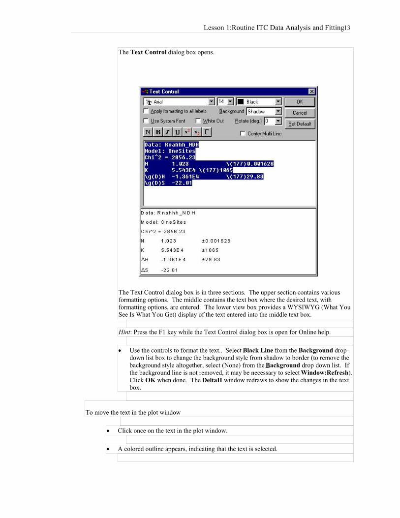
The Text Control dialog box opens.
The Text Control dialog box is in three sections. The upper section contains variousformatting options. The middle contains the text box where the desired text, withformatting options, are entered. The lower view box provides a WYSIWYG (What YouSee Is What You Get) display of the text entered into the middle text box.
Hint: Press the F1 key while the Text Control dialog box is open for Online help.
Use the controls to format the text.. Select Black Line from the Background drop-down list box to change the background style from shadow to border (to remove thebackground style altogether, select (None) from the Background drop down list. Ifthe background line is not removed, it may be necessary to select Window:Refresh).Click OK when done. The DeltaH window redraws to show the changes in the textbox.
To move the text in the plot window
Click once on the text in the plot window.
A colored outline appears, indicating that the text is selected.

Click and drag within the colored outline to move the text.
Click outside the colored outline to deselect the text.
Hint: If you click anywhere along the edge of the text background border, a colored sizebox appears around the text with various size boxes positioned around the perimeter.Click and drag on one of the small perimeter boxes to change the size of the textbackground frame. (Note: Origin will not allow you to size the background bordersmaller than will display the complete text, if you wish a smaller box size than allowedyou must reduce the font size of the text.)
Note that any formatting changes can be saved as part of the DeltaH plot windowtemplate file. See page PAGEREF modify_and_save \h 49 for details.
To view the Results Window
When fitting is done the fitting parameters are routed to the text window namedResults and the window is then minimized (it may be restored by selectingWindow : Results). (The Results Window is a Text window where you can edit orprint the text or copy all or part of the text to the plot window or to another textediting program.)
EMBED PBrush

Lesson 1:Routine ITC Data Analysis and Fitting15
Creating a Final Figure for Publication
To create a final figure for publication, select Final Figure from the ITC menu. TheITCFINAL plot window opens. This window contains two related graphs. The topgraph shows raw data in terms of mcal/second plotted against time in minutes, after theintegration baseline has been subtracted. The bottom graph shows normalizedintegration data in terms of kcal/mole of injectant plotted against molar ratio. The two Xaxes are linked, so that the integrated area for each peak appears directly below thecorresponding peak in the raw data.
-40
-20
0
0 10 20 30 40
Time (min)
µcal
/sec
0.0 0.5 1.0 1.5 2.0-14
-12
-10
-8
-6
-4
-2
0
Molar Ratio
kcal
/mol
e of
inje
ctan
t
If you modify the integration data or the fit curve in the DeltaH window, or the raw datain the RawITC window, simply select Final Figure again to update the ITCFINALwindow with your changes.
Note that the top graph in the ITCFINAL window still includes the integration baselineat Y = 0. You may wish to remove this baseline before printing the graph.
To remove the baseline from the raw data
Origin has drawn a red baseline (rnahhhbase) for the raw data at Y = 0. If you like, youcan remove this baseline as follows:

1. Double-click on the baseline. The Plot Details dialog box opens.
2. In the Plot Details dialog box, click on the Remove button. The dialog box closes, andthe baseline data are removed from the project. (Note: You may remove the baseline fromthe plotted data, by double-clicking on the Layer Control button in the upper left cornerof the ITCFinal window, and then move the rnahhhbase data from the Layer Contents listto the Available Data list by first highlighting it and then selecting the left-pointingarrow.)
To paste the fitting parameters to the ITCFinal window
Earlier in this lesson the fitting parameters were pasted to the DeltaH window. Beforeprinting, let's copy these parameters and paste them to the ITCFINAL window.
1. Click on the DeltaH window, or select DeltaH from the Window menu. DeltaHbecomes the active window.
2. Click on the fitting parameters text label we had placed in the upper-left corner of thewindow. A colored selection square surrounds the text.
Shortcut: Right-clickanywhere inside the axisof the graph and selectPlot Details …

Lesson 1:Routine ITC Data Analysis and Fitting17
3. Select the Edit:Copy command.
4. Click on the ITCFINAL window, or select ITCFinal from the Window menu.ITCFINAL becomes the active window. Click once on a position in the graph whereyou want the parameter box to appear.
5. Select the EDIT:PASTE command. The fitting parameters paste to the ITCFINALwindow.
6. We want to position the text label next to the integration data, but first we need toreduce the size of the label. Double click on the text label to open the Text Controldialog box. Select 8 (or type 8) in the center drop-down list to reduce the point size to 8.Click OK to close the dialog box.
7. Click and drag the label to position it next to the integration data, as shown below:
_________________________________________________________________________ Note: The user should understand that the "raw data" in the upper frame of the ITCFinal template isthe original raw data after the integration baseline has been subtracted from it. Once this subtractionhas been made by creating the ITCFinal figure, there is no way to recover the original raw data exceptby starting a new project and calling in the raw data file again, since the subtracted data has beenstored under the original filename and the original integration baseline replaced by the Y=0 baseline.________________________________________________________________________
Alternatively, tocopy and paste, youmay right-clickanywhere inside thetext box, select copythen right-clickwhere you want toposition the textlabel and selectpaste.
-40
-20
0
0 10 20 30 40
Time (min)
µca
l/sec
0 .0 0 .5 1.0 1 .5 2.0
-14
-12
-10
-8
-6
-4
-2
0
Data: Rnahhh_NDH
M odel: OneSites
Chi^2 = 2856.23
N 1.023 ± 0.001628
K 5.543E4 ± 1065
H -1.361E4 ± 29.83
S -22.01
Molar Ratio
kcal
/mol
e of
inje
ctan
t

To print the final figure
To print the page in the ITCFINAL window, select Print from the File menu. Beforeyou print, make sure ITCFINAL is the active window. When a window is active its titlebar changes from gray to blue (this can vary depending on your Windows setup, to viewor change your setup select Start:Settings:Control Panel then double click on Display andclick on the Appearance tab). Click on a window to make it active, or select the windowfrom the Window List in the Window menu.
To save the project and exit
Choose Save Project As... from the File menu.The file Save As dialog box opens.
Enter a name for the project (for example, Lesson 1) in the File Name text box. New toWindows 95 the name for the project may contain up to 255 characters and includespaces.
Click on the OK button.The entire contents of this project (including all data sets and plot windows) are savedinto a file called Lesson 1.OPJ.
Choose Exit from the File menu.Origin closes.
Shortcut:Click the SaveProject button onthe Standardtoolbar.
EMBEDPBrus

Lesson 2: Setting Baseline and integration Range
Lesson 2: Setting Baseline and Integration Range
In Lesson 1 you learned how to use Origin to perform routine data analysis of ITC files.In routine data analysis, integration details (baselines and integration ranges) aredetermined automatically. Sometimes, however, the automatically determined values arenot sufficiently accurate, and you will want to set integration details manually. This isespecially true when working with very small injection peaks. This lesson shows you howto manually set integration details.
Begin this lesson by starting Origin, then opening the RNAHHH. ITC data file, as you didat the beginning of Lesson 1.
To start Origin
Double-click on the Origin for ITC icon on the DeskTop. (If the icon is not available onthe DeskTop, Start from the task bar, then select Programs:MicroCalOrigin50:MicroCal Inc. ITC).
Origin opens and displays a new project with the RawITC template plot window.
To open the RNAHHH file
Click on the Read Data button. The Open dialog box opens, with the ITC Data (*.it?)file name extension selected.
If you have not previously Set Default Folder... to the samples subfolder, then navigateto the C:\Origin50\samples subfolder.
Select Rnahhh from the Files list.
Click OK.
Raw data are plotted in the RawITC window. Normalized area data are plotted in theDeltaH window.
Select the RawITC window from the file list in the Window menu.
Note: If you ever notice that the the RawITC window , or another window, has lost someof its formatting instructions (e.g., text rotation), this can happen from being in the DraftView mode. Draft View is the fastest view mode, and is very useful when preciseformatting is not required. The View Mode is selected from the Page menu. To view thepage as it will appear when printed, select Page View mode which is the slowest but mostaccurate. Page View mode is often the most useful, since it combines reasonably goodWYSIWYG accuracy with fast operation. (also see Origin User’s Manual or Origin’sHelp menu item, for more information on view mode).
To enter the Adjust Integration session
Click on the Adjust Integrations button in the RawITC window. The cursor changesinto a cross hair.

Move the cursor into the RawITC plot window and click on or near the injection peakyou want to adjust. For this example, click on peak 19 (second peak from the right). Thewindow zooms to shows the baseline region of peaks 18, 19 and 20. (Note: Origin willshow the injection peak before and the injection peak after the injection chosen, but anymanipulations will only affect the integrated area in the center injection)
A new set of buttons appears along the top edge of the window. Two dashed blue linesappear, the section of the plot between the lines is the integration range.
The basic procedure for adjusting integration details is to select a peak, adjust the baseline and theintegration range, integrate the peak, and then move on to the next peak and repeat the process.The expanded screen is shown below.
To adjust the baseline
Click on the Baseline button in the RawITC window (which has been temporarily titledPeak 19).The automatically generated points for this baseline appear. (For the baseline, Origin displays 15 points which includes the central peak and eachneighboring peak. In most cases you may want to adjust only the central five points forthe central peak of interest. The outermost points are usually more closely associatedwith the neighboring peaks.
Click on a point, then drag the mouse or use the and keys to move the point (note thatbaseline points can only move vertically). Use the and keys (or the mouse) to selectthe next point to the right or left. Repeat for each point you want to move.
Note: When any point on the baseline is moved, the position of the moved pointautomatically becomes part of the baseline and any future integration will be calculatedfrom this new baseline.
Lesson 2: Setting Baseline and integration Range
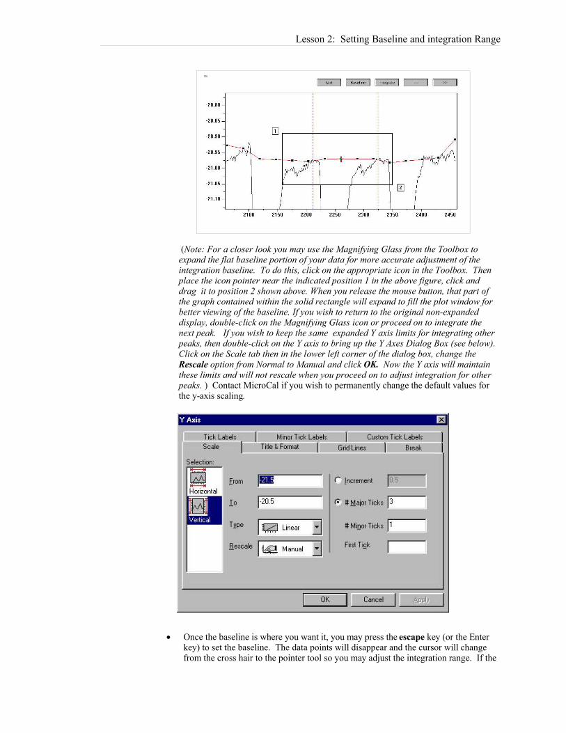
(Note: For a closer look you may use the Magnifying Glass from the Toolbox toexpand the flat baseline portion of your data for more accurate adjustment of theintegration baseline. To do this, click on the appropriate icon in the Toolbox. Thenplace the icon pointer near the indicated position 1 in the above figure, click anddrag it to position 2 shown above. When you release the mouse button, that part ofthe graph contained within the solid rectangle will expand to fill the plot window forbetter viewing of the baseline. If you wish to return to the original non-expandeddisplay, double-click on the Magnifying Glass icon or proceed on to integrate thenext peak. If you wish to keep the same expanded Y axis limits for integrating otherpeaks, then double-click on the Y axis to bring up the Y Axes Dialog Box (see below).Click on the Scale tab then in the lower left corner of the dialog box, change theRescale option from Normal to Manual and click OK. Now the Y axis will maintainthese limits and will not rescale when you proceed on to adjust integration for otherpeaks. ) Contact MicroCal if you wish to permanently change the default values forthe y-axis scaling.
Once the baseline is where you want it, you may press the escape key (or the Enterkey) to set the baseline. The data points will disappear and the cursor will changefrom the cross hair to the pointer tool so you may adjust the integration range. If the

integration range is already set you may click on the Integrate button and click on anarrow key to show an adjacent peak
To adjust the integration range
If the baseline data points are still visible double-click on any data point or press theEnter key or press the Esc key.The data points will disappear and the cursor will change from the cross-hair to thepointer tool.
Set a new integration range by clicking and dragging either line with the mouse.
The integration area for the central peak selected will be between the dashed blue lines.
To integrate the selected peak
Click on the Integrate button.This integrates the peak, using the current baseline and integration range. The curve inthe DeltaH window is updated accordingly. The integration results are also updated onthe worksheet containing the injection data.
To select another peak
Click on the and buttons to move to the next or
previous peak. Note that the current peak number is always displayed in the window titlebar.
To end the Adjust Integration session
Click on the Quit button. The RawITC window is restored to show all of the injection peaks. Note that the areadata in the DeltaH window will have updated to reflect any changes you made.

Lesson 2: Setting Baseline and integration Range
You will notice that the RawITC template includes a button to Integrate All Peaks. Thisbutton integrates all injection peaks and replots the area data. You will recall from theprevious lesson that the area data in the DeltaH window were originally created with theIntegrate All Peaks routine.
It is not necessary at this point to integrate on all peaks again. In fact, it is a good idea not to.If you now integrate on all peaks, you will not get the same area result as when you integratedeach peak separately.
To view the worksheet data
Select the Pointer tool by clicking on it in the Toolbox.
Double-click anywhere on the trace of the RawITC data plot in the plot window or selectFormat : Plot. The Plot Details dialog box opens for this data plot.
Click on the Worksheet button.The Worksheet containing the injection data opens.
Note: You may notice that the worksheet X axis values are in seconds, while the plotted datais shown in minutes. This is because the X axis has been factored, as described in Lesson 6.
You can now proceed to fit the data (see Lesson 1). If necessary, you can first delete any baddata points, as descried in the next lesson.
Shortcut to theWorksheet: Right-clickanywhere on the datatrace and select OpenWorksheet.

Lesson 3: Deleting Bad Data
After your injection data are integrated, the integration results are displayed in theDeltaH plot window. You can delete bad data points from the DeltaH window beforestarting the fitting session.
To delete bad data points
Select Window : DeltaH to make it the active window.
Click on the Remove Bad Data button.The pointer becomes a cross-hair.
Click on the point that you want to delete.A small red cross appears on the selected data point.The XY coordinates, index number, and data set name for the selected point aredisplayed immediately in the Data Display Tool (floating).
Note: If you have trouble selecting a particular data point, select a point near by and usethe left or right arrow keys to move to the data point you wish to select.
Press ENTER.The selected data point is deleted. Alternatively, after clicking on Remove Bad Data,you may double click on a data point to delete it.
Note: The main menu bar also contains a data deletion function under Data: RemoveBad Data Points… and this works a little differently. We recommend the user alwaysdelete data using the Remove Bad Data button located on the DeltaH plot window.
Though there is no Undo command available in this version of Origin with which to un-delete a data point, it is possible to recover if you have mistakenly deleted a point. Torecover, simply integrate the injection peaks again (by clicking on the Integrate AllPeaks button in the RawITC window). All of the injection peaks will re-integrate, andthe area data, including the deleted data point, will replot in the DeltaH window. Asecond way to recover the bad point, without reintegrating, is to click on theConcentration button and then click OK. Even if you did not change the concentration inthe dialog box, Origin goes back to the worksheet and normalizes on the concentrationagain which then restores the deleted point.
Shortcut to switchbetween Originwindows: Press andhold down the Ctrlkey while pressingthe Tab key.

Shortcut: Click theNew Projectbutton on theStandardtoolbar.
Lesson 4: Analyzing Multiple runs and subtracting Reference
Lesson 4: Analyzing Multiple Runs and Subtracting Reference
Origin allows you to open multiple runs of ITC data into the same project, and subtractone run from another. The heat of ligand dilution into buffer can thus be subtracted fromthe reaction heat by performing the control experiment of injecting into a buffer solution,and subtracting this reference data from the reaction heat data.
In order to subtract the reference injections, you must have both the sample and referencearea data in memory. This lesson shows you how to read two area data files into Originand subtract one from the other. In the first example below you will read two area (.DH)data files from disk. In the second example, you will work directly with two raw (*.ITC)ITC data files. This second example also illustrates some helpful procedures for dealingwith difficult data
Two reference data files, BUFFER.DH and FEBUF10.ITC, have been included in the[samples] subfolder for your use with this lesson.
Before you begin this lesson, open a new project. This will clear any old data that maybe in memory.
To open a new project
Choose Project from the New sub-menu under the File menu.
Opening Multiple Data Files
In the following example you will open two area (.DH) data files and subtract one fromthe other. Both area files were previously saved to disk. This example assumes that youhave previously opened the ITC file Rnahhh.itc into Origin, and saved the resulting areadata as Rnahhh.DH, as described in Lesson 1. If you have not yet done so, you shouldrefer to Lesson 1 now.
To read the sample and reference data into memory
Click on the Read Data.. button in the RawITC plot window.The File Open dialog box opens click on the down arrow in the Files of type: drop-down list box and select Area Data (*.DH).
SYMBOL 183 \f "Symbol" \s 10 \h Navigate to the [Origin50][samples] subfolder.Several .DH files will be listed in the File Name text field.
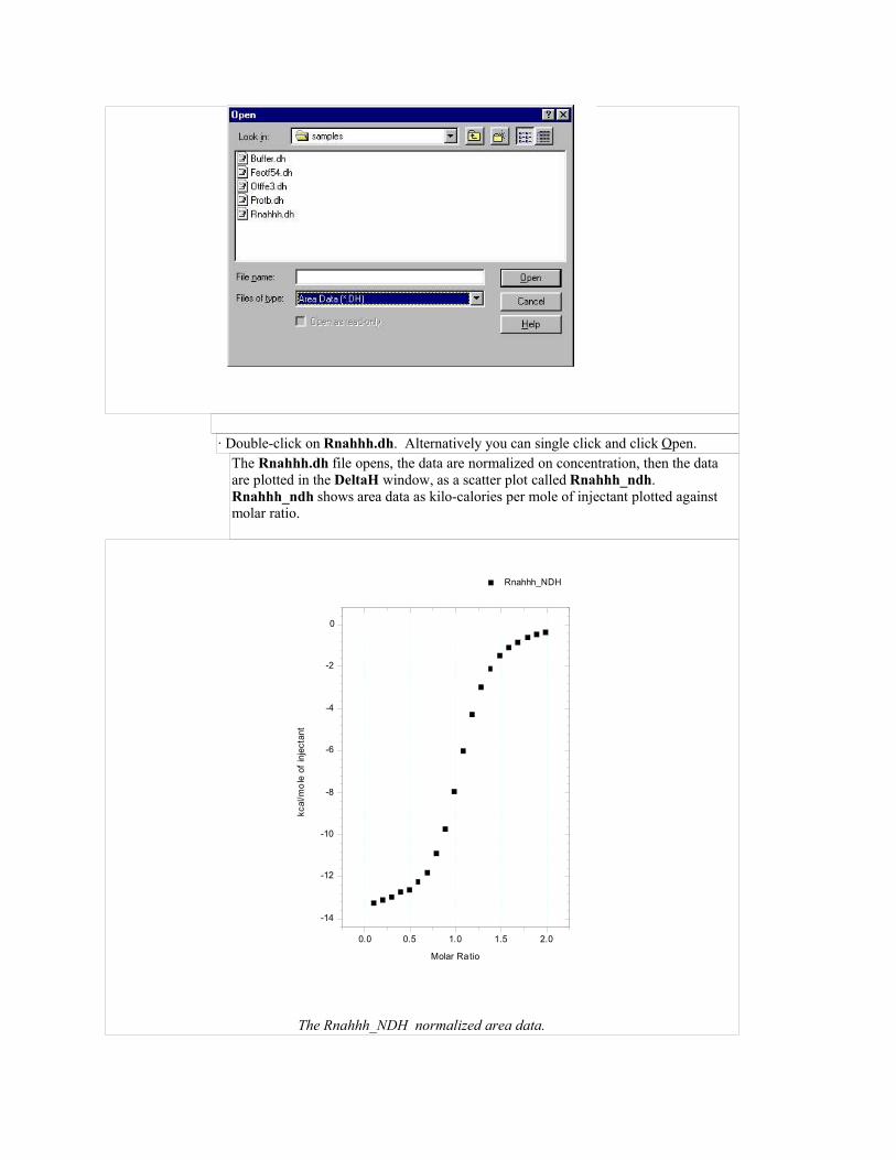
· Double-click on Rnahhh.dh. Alternatively you can single click and click Open.The Rnahhh.dh file opens, the data are normalized on concentration, then the dataare plotted in the DeltaH window, as a scatter plot called Rnahhh_ndh.Rnahhh_ndh shows area data as kilo-calories per mole of injectant plotted againstmolar ratio.
The Rnahhh_NDH normalized area data.
0.0 0.5 1.0 1.5 2.0
-14
-12
-10
-8
-6
-4
-2
0
Rnahhh_NDH
Molar Ratio
kcal
/mol
e of
inje
ctan
t
Lesson 4: Analyzing Multiple runs and subtracting Reference
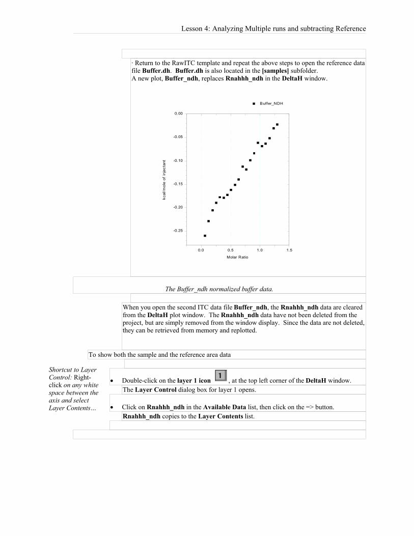
· Return to the RawITC template and repeat the above steps to open the reference datafile Buffer.dh. Buffer.dh is also located in the [samples] subfolder.A new plot, Buffer_ndh, replaces Rnahhh_ndh in the DeltaH window.
The Buffer_ndh normalized buffer data.
When you open the second ITC data file Buffer_ndh, the Rnahhh_ndh data are clearedfrom the DeltaH plot window. The Rnahhh_ndh data have not been deleted from theproject, but are simply removed from the window display. Since the data are not deleted,they can be retrieved from memory and replotted.
To show both the sample and the reference area data
Double-click on the layer 1 icon , at the top left corner of the DeltaH window.The Layer Control dialog box for layer 1 opens.
Click on Rnahhh_ndh in the Available Data list, then click on the => button.Rnahhh_ndh copies to the Layer Contents list.
Shortcut to LayerControl: Right-click on any whitespace between theaxis and selectLayer Contents…
0.0 0.5 1.0 1.5
-0.25
-0.20
-0.15
-0.10
-0.05
0.00
Buffer_NDH
Molar Ratio
kcal
/mol
e of
inje
ctan
t

Click OK.Rnahhh_ndh plots into the DeltaH window. The axes automatically rescale to show allof the data.
Rnahhh_ndh and Buffer_ndh, plotted together.
The Available Data list in the Layer Control dialog box shows all data sets currentlyavailable for plotting in this project. The Layer Contents list shows all data setscurrently plotted in the active layer. See the Origin User’s Manual or Origin's OnlineHelp menu item (or press F1) for more on handling Origin data.
Note that you can read any number of data files into the same DeltaH window. Whenmultiple data plots appear in the same window, you can set the active data plot byclicking on the plot type (line/symbol) icons next to the data set name in the legend:
0.0 0.5 1.0 1.5 2.0
-14
-12
-10
-8
-6
-4
-2
0
Buffer_NDH
Rnahhh_NDH
Molar Ratio
kcal
/mol
e of
inje
ctan
t

Lesson 4: Analyzing Multiple runs and subtracting Reference
A black border around the line/symbol icon indicates thecurrently active data plot. Editing, fitting, and otheroperations can only be carried out on the active plot.
Adjusting the Molar Ratio
Note in the above figure that the Buffer_ndh data plots from molar ratio 0 to ca. 1.3,while the Rnahhh_ndh data plots from 0 to ca. 2.0. In the case of the Buffer_ndh data,the molar ratio is in fact infinity since injections of 21.16 mM ligand solution were madeinto a cell which contained only buffer and no macromolecule (i.e., in order to determineheats of dilution of ligand into buffer).
Origin automatically assigns a concentration of 1.0 mM in order to obtain non-infinitevalues for the molar ratio to allow plotting of the Buffer_ndh points. Before subtractingthe reference data you should check that the molar ratio is identical for both data sets.This will ensure that the final result is accurate, and will also ensure that the two data setsplot in register (that is, injection #1 of the control experiment plots at the same molarratio as injection #1 of the sample experiment, etc.).
To adjust the molar ratio
1. Click on the Data menu, and check that Rnahhh is checkmarked. If not, selectRnahhh from the menu. This sets Rnahhh as the active data set.
(as a simpler alternative to the above procedure, you could have just clicked on the Rnahhh_NDH listing in the plot type icon.
2. In the DeltaH window, click on the Concentration button. In the dialog box thatopens, note the value in the C in Cell (mM) field (it should be .651).
3. Click Cancel to close the dialog box. Now repeat step 1, but this time set the Bufferdata set as active.
4. In the DeltaH window, click again on the Concentration button. This time a dialogbox opens to show the concentration values for Buffer. In the C in Cell (mM) field,enter .651. Click OK. The two data sets will now plot in register, as shown below:
EMBED PBrush
Alternatively you mayright-click on anyopen space betweenthe axis and click onRnahhh
EMBED PBrush

Subtracting Reference Data
To subtract Buffer_ndh from Rnahhh_ndh
Click on the Subtract Reference Data.. button in the DeltaH window.The Subtract Reference Data dialog box opens. The most recent file opened, in thiscase Buffer_NDH, will appear in both the Data and Reference drop down list box. Notethat the data set in the Reference box will be subtracted from the data set in the Data box.
Select Rnahhh_NDH from the Data drop down list.Rnahhh_NDH becomes highlighted and will be entered as the Data.

Lesson 4: Analyzing Multiple runs and subtracting Reference
Click OK.Every point in Buffer_ndh is subtracted from the corresponding point in Rnahhh_ndh.The result is plotted as Rnahhh_ndh in the active layer, in this case layer 1 in theDeltaH plot window.
Note that Buffer_ndh is not affected by this operation. It is cleared from the DeltaHwindow, but is still listed as available data in the Layer Control dialog box. TheOriginal Rnahhh_ndh data could be recovered by selecting Math : Simple Math andadding the Buffer_ndh data set to the new Rnahhh_ndh data set.
To save the project and all related data files
SYMBOL 183 \f "Symbol" \s 10 \h Select the File:Save Project As command from theOrigin menu bar.The Save As dialog box opens, with untitled selected as the file name.
0.0 0.5 1.0 1.5 2.0-14
-12
-10
-8
-6
-4
-2
0
Rnahhh_NDH
###
Molar Ratio
kcal
/mo
le o
f in
ject
ant

SYMBOL 183 \f "Symbol" \s 10 \h Enter a new name (Origin50 accepts long filenames)for the project, navigate to the folder in which you want to save the file, and click OK. Itis not necessary to enter the .opj file extension. This will be added automatically. Nowthat you have named the file, the next time you save it you can simply use the File:SaveProject command.
In order to save some memory space, you may find it useful to delete the originalinjection data. This may be useful when you are reading a large number of data sets intothe same Origin project.
To delete a data set from a project, either
Double-click on any layer icon in any plot window.
Select a data set from the Available Data list, then click on the Delete button.
or
If the data are plotted in a plot window, double-click on the trace of the data plot that youwant to delete.
The Plot Details dialog box opens. The name of the data set appears in the top leftcorner of the dialog box.
Click on the Remove button.
In either case the data set, along with any related data plots, is deleted from the project.If you have saved the data set to disk, the saved copy will not be affected.
Plotting Multiple Data Sets
Whenever multiple data sets are included in the same plot, there may be overlap of datapoints from the different data sets. There are two ways to eliminate this overlap bydisplacing one or more of the curves on the Y axis if you wish to do so. First, you mayselect Math : Simple Math and add or subtract a constant from all points in one data setto displace it. Remember if you are doing this on data plotted in the DeltaH template thatalthough data is plotted in kcal, the actual data is in the worksheet as cal so they must bemodified by adding or subtracting cal (see A Note about Units starting on pagePAGEREF units \h 53). Second, you may make the appropriate data set active byselecting it in the list for plot type icons. Then select Math : Y Translate. Use theresulting icon to select one data point in the active set , click on it, and hit enter (ordouble click on a data point). Then move the icon to the Y position on the graph whereyou wish that point to be after displacement, click on it and hit enter. The entire data setwill be translated on the Y axis by that amount.
Subtracting Reference Data: Additional Topics
In the previous example, the sample injection data and reference injection data matchedprecisely. This may not always be the case, however. Your reference data may have a

Lesson 4: Analyzing Multiple runs and subtracting Reference
different number of injections than your sample data, or the injection time spacing maydiffer between the two runs. You will see below how to deal with these situations.
In the following example you will open two ITC raw (*.ITC) data file series, onecontaining the sample data and one containing the reference data. You will then plot thearea data for each data file series, and subtract reference data from sample data.Begin by opening a new project:
Select Project from the New sub-menu under the File menu.
To open both sample and reference raw data files
Click on the Read Data.. button in the RawITC window and select ITC Data (*.it?)from the Files of type: drop down list box.
Double-click on Rnahhh in the File Name list (located in the [Origin50][samples]subfolder).
The Rnahhh.itc file opens.The data are integrated, normalized, and the area data plots in the DeltaH window.
Return to the RawITC window and repeat the above steps to open the Febuf10.itc datafile.
The Febuf10_ndh area data replaces Rnahhh_ndh in the DeltaH window. You need toplot both area data sets into layer 1.
To show both area data sets in layer 1
Double-click on the layer 1 icon in the DeltaH plot window.The Layer Control dialog box opens.
Select Rnahhh_ndh in the Available Data list, then click on the => button.Rnahhh_ndh joins Febuf10_ndh in the Layer Contents list.
Click OK.Rnahhh_ndh joins Febuf10_ndh in the DeltaH plot window.The axes automatically rescale to show all the data. Your plot window should now looklike the illustration below:

As we discussed earlier in this lesson (page PAGEREF ConcentrationCheck \h 31), youshould now check that the ligand concentrations for both data sets are identical. Makeeach data set active in turn, then click on the Concentration button in the DeltaHwindow, and check that value in the C in Cell (mM) field for Febuf10_ndh is identical tothat value for Rnahhh_ndh. In this case, you will find that the two values are the same.
Notice that Febuf10_ndh shows only twelve injections, while Rnahhh_ndh showstwenty. How do you subtract one data set from another when the number of injectionsdoesn't match? The quick and dirty way is to subtract a constant. A more precise methodwould be to fit a straight line to the reference data, then subtract the line. Let's lookbriefly at each method.
To subtract a constant from Rnahhh_ndh
Select the Data Reader tool from the toolbox.The pointer changes to a cross-hair.
Click the mouse on several different data points in the Febuf10_ndh data series in theDeltaH window, each time noting the Y value that appears in the Data Display.
EMBED PBrush

Lesson 4: Analyzing Multiple runs and subtracting Reference
Using these Y values, figure a rough average for the data. For this example, let's say theaverage Y value is 350 (See Calculating a Mean Value for Reference Data starting onpage PAGEREF CalculatingMean \h 71 for a method to quickly calculate a mean of thedata). (Note that the Data Reader tool shows values in calories, while the Y axis in thisgraph shows values in kcal. This is because the Y axis in the DeltaH plot windowtemplate is factored by a value of 1000. See Lesson 6 for more about factoring.)
Select Simple Math from the Math menu.The Math on/between Data Set dialog box opens.
Select Rnahhh_ndh from the Available Data list, then click on the uppermost =>button.
Rnahhh_ndh copies to the Y1 text box. Rnahhh_ndh also appears next to Y:. Y:indicates the name of the data set into which the resulting data will be copied.
Click in the Y2 text box and type " 350 " at the insertion point.
Click in the operator box, and type " - " at the insertion point.
Click OK.The constant "350" is subtracted from each value in the Rnahhh_ndh data set. Theresult is plotted as Rnahhh_ndh in the DeltaH window.
To subtract a straight line from RNAHHH_NDH
Click on the Pointer tool to deselect the Screen Reader tool. Now check theData menu to see that Febuf10_ndh is the active data set (the active data set will becheckmarked). All editing, and fitting operations are carried out on the active data set.Select Febuf10_ndh if it is not active.

Select Linear Regression from the Math menu.A straight line is fit to the Febuf10_ndh data. Origin assigns the nameLinearFit_Febuf10ND to the data set for this line.The Results window opens to display the fitting parameters. This can be a usefulfeature, but we are not interested in the fitting parameters right now. To close the ResultsWindow, select Minimize Window button located in the upper right handcorner of the window.
Select Simple Math from the Math menu.The Math dialog box opens.
EMBED PBrush
EMBED

Lesson 4: Analyzing Multiple runs and subtracting Reference
Select Rnahhh_NDH from the Available Data list, then click on the uppermost =>button.Rnahhh_NDH copies to the Y1 text box.
Select LinearFit_Febuf10ND from the Available Data list, then click on the lowermost=> button.LinearFit_Febuf10ND copies to the Y2 text box.
Click in the operator box and type " - ".
Click OK.Every point in LinearFit_Febuf10ND is subtracted from the corresponding point inRnahhh_ndh. The resulting data set is plotted as Rnahhh_ndh in the DeltaH plotwindow. Note that the Febuf10_ndh reference data plot (the original twelve injectionpoints) is not affected.
We will end this lesson with a note about injection timing. You may have noticed thedifference in injection time spacing between Rnahhhraw_cp and Febuf10raw _cp. Tomake this difference more apparent you need to plot both raw data sets in the same plotwindow.
EMBED PBrush
EMBED PBrush
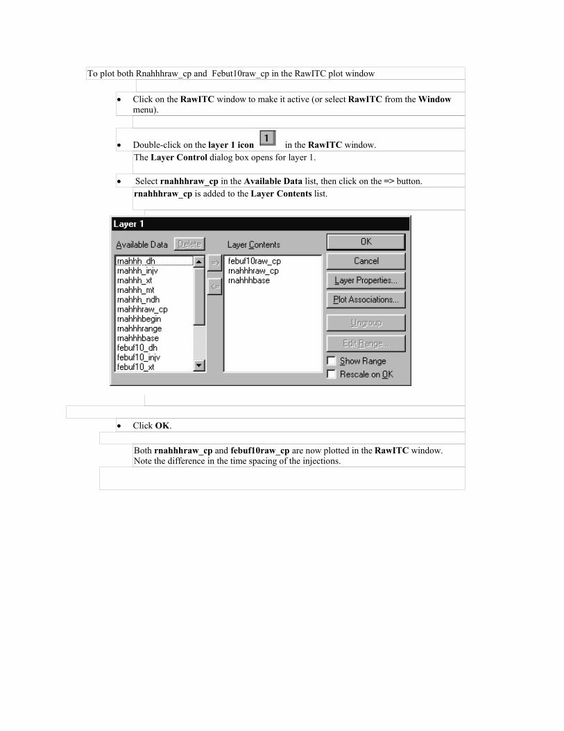
To plot both Rnahhhraw_cp and Febut10raw_cp in the RawITC plot window
Click on the RawITC window to make it active (or select RawITC from the Windowmenu).
Double-click on the layer 1 icon in the RawITC window.The Layer Control dialog box opens for layer 1.
Select rnahhhraw_cp in the Available Data list, then click on the => button.rnahhhraw_cp is added to the Layer Contents list.
Click OK.
Both rnahhhraw_cp and febuf10raw_cp are now plotted in the RawITC window.Note the difference in the time spacing of the injections.
Lesson 4: Analyzing Multiple runs and subtracting Reference
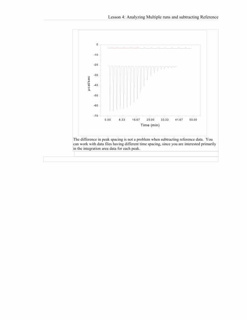
The difference in peak spacing is not a problem when subtracting reference data. Youcan work with data files having different time spacing, since you are interested primarilyin the integration area data for each peak.
0.00 8.33 16.67 25.00 33.33 41.67 50.00-70
-60
-50
-40
-30
-20
-10
0
Time (min)
µca
l/sec

Lesson 5: ITC Data Handling
Every data plot in Origin has an associated worksheet. The worksheet contains the X, Yand, if appropriate, the error bar values for the plot. A worksheet can contain values formore than one data plot.
It is always possible to view the worksheet from which data were plotted. This lessonshows you how to open the worksheet associated with a particular data plot, copy/pastethe data, export the data to an ASCII file, and import ASCII data.
Reading Worksheet Values from Plotted Data
Begin this lesson by opening the ITC Rnahhh.ITC data file series, as follows:
Select File : New : Project.A new Origin project opens to display the RawITC plot window.
Click on the Read Data.. button.The File Open dialog box opens, with the ITC Data (*.IT?) file name extensionselected.
If you have not previously Set Default Folder... to the samples folder, then navigate tothe C:\Origin50\samples folder.
Select Rnahhh from the file name list, and click OK.
As you saw in Lesson 1, Origin plots the Rnahhh data as a line graph in the RawITCplot window, automatically creates a baseline, integrates the peaks, normalizes theintegration data, and plots the normalized data in the DeltaH plot window. As a result,the following eight data sets are created:
rnahhh_dh Experimental heat change resulting from injection i, inmcal/injection (not displayed).
rnahhh_mt Concentration of macromolecule in the cell before eachinjection i, after correction for volume displacement (notdisplayed).
rnahhh_xt Concentration of injected solute in the cell before eachinjection (not displayed).
rnahhh_injv Volume of injectant added for the injection i.rnahhh_ndh Normalized heat change for injection i, in calories per mole of
injectant added (displayed in DeltaH window).rnahhh_xmt Molar ratio of ligand to macromolecule after injection i (X
value of data point).rnahhhbase Baseline for the injection data (displayed in red in the
RawITC window).rnahhhraw_cp All of the original injection data (displayed in black in the
RawITC window).
Shortcut: Select theNew Project button.
EMBEDPBru
Lesson 5: ITC Data Handling
In addition origin creates two temporary data sets:
rnahhhbegin Contains the indices (row numbers) of the start of an injection.
rnahhhrange Contains the indices of the integration range for the injections.
An Origin data set is named after its worksheet and worksheet column, usually separatedby an underscore. Thus the first six data sets above will all be found on the sameworksheet (RNAHHH), in columns named DH, INJV, Xt, Mt, XMt and NDH,respectively. The temporary two data sets above are located on separate worksheets,named rnahhhbase (an Origin created baseline) and RnahhhRAW (the experimentaldata). The temporary data sets are indices created by Origin and do not have a worksheetcreated.
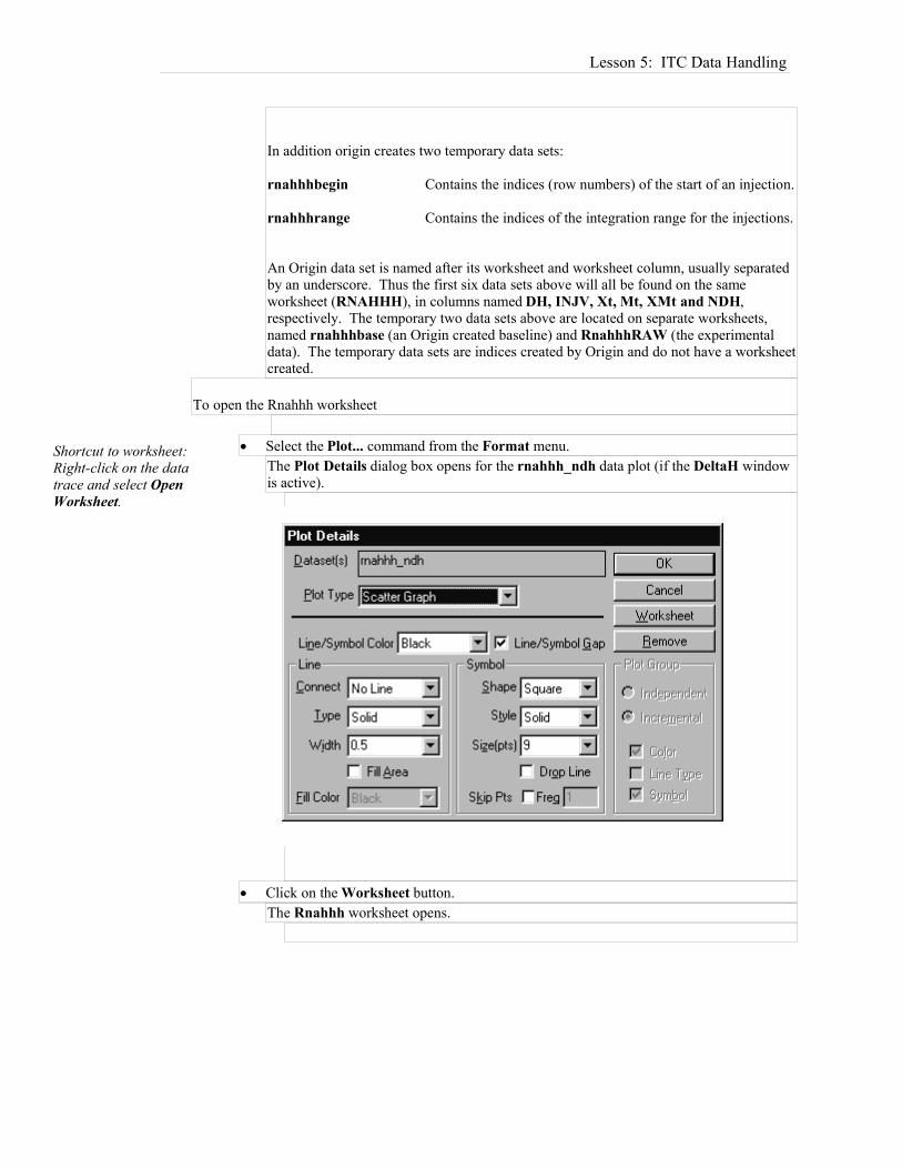
To open the Rnahhh worksheet
Select the Plot... command from the Format menu.The Plot Details dialog box opens for the rnahhh_ndh data plot (if the DeltaH windowis active).
Click on the Worksheet button.The Rnahhh worksheet opens.
Shortcut to worksheet:Right-click on the datatrace and select OpenWorksheet.

Copy and Paste Worksheet Data
Data can be copied from a worksheet to the clipboard, then pasted from the clipboardinto another Origin worksheet, a plot window, or another Windows application. To copyand paste worksheet data:
Select a range of worksheet values
Select the initial cell, row, or column in the range.To select a cell, click on the cell. To select an entire row, click on the row number. Toselect an entire column, click on the column heading.
To select a contiguous portion of worksheet values, click on the first cell, row or column,keep the mouse button depressed, drag to the final cell, row, or column that you want toinclude in the selection range, then release the mouse button. The entire selection rangewill now be highlighted. (Note: If you ever wish to select a range of cells where theinitial cell but not the final cell is in view, then click on the first cell and scroll to the finalcell, press and hold the shift key then click the final cell.
Copy the selected values to the clipboard
Choose Copy from the Edit menu, alternatively you may click the right mouse buttoninside the highlighted text and select Copy from the menu.The selected values are copied to Windows clipboard.
Select a destination for the copied values
To paste into a plot window, click on the plot window to make it active.
EMBED PBrush
EMBEDPBrus

Lesson 5: ITC Data Handling
To paste into a worksheet, click on the worksheet (or select File:New:Worksheet toopen a new worksheet), then click to select a single cell. This cell will be in the upperleft corner of the destination range.
To paste into another Windows application, switch to the target application, then followthe pasting procedure for that application.(Shortcut: If an application is already open you may switch to it by pressing and holdingdown the Alt key then pressing the Tab key till the application's icon is selected.
Paste the copied values from the clipboard to the destination
Select Paste from the Edit menu, alternatively click the right mouse button and selectPaste.The selected values are pasted from the clipboard.
Before you proceed, minimize the Rnahhh worksheet.
To minimize a worksheet window
Click on the Minimize Window button located in the upper right corner of theworksheet window.
Exporting Worksheet Data
The contents of any worksheet can be saved into an ASCII file. In this section you willopen the worksheet for the RnahhhBASE baseline data plotted in the RawITC window,and export the X and Y data to an ASCII file.
To open the Rnahhhbase worksheet
Click on the RawITC window (or choose RawITC from the Window menu) to make itthe active window.
Select RnahhhBASE from the Data menu.RnahhhBASE becomes checkmarked to show it is selected.
Select Plot... from the Format menu.
EMBED PBrush
Shortcut:To open a newworksheet click onthe New Worksheetbutton from theStandard toolbar.
Shortcut toworksheet:Right-click on thedata trace and selectOpen Worksheet.
EMBED

The Plot Details dialog box opens.
Click on the Worksheet button.The RnahhhBASE worksheet opens.
To export the worksheet data as an ASCII file
Select Export ASCII... from the File menu.The Export ASCII dialog box opens, with RnahhhBASE.DAT selected as the filename.
Click Save.
EMBED PBrush
Shortcut: Right-click on theupper left containingwhite-space thenselect Export ASCII.
Lesson 5: ITC Data Handling
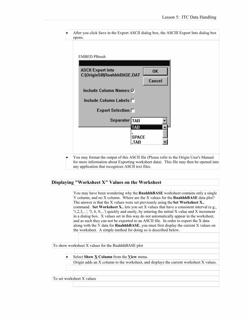
After you click Save in the Export ASCII dialog box, the ASCIII Export Into dialog boxopens.
You may format the output of this ASCII file (Please refer to the Origin User's Manualfor more information about Exporting worksheet data). This file may then be opened intoany application that recognizes ASCII text files.
Displaying "Worksheet X" Values on the Worksheet
You may have been wondering why the RnahhhBASE worksheet contains only a singleY column, and no X column. Where are the X values for the RnahhhBASE data plot?The answer is that the X values were set previously using the Set Worksheet X..command. Set Worksheet X.. lets you set X values that have a consistent interval (e.g.,'1,2,3,...', '3, 6, 9,...') quickly and easily, by entering the initial X value and X incrementin a dialog box. X values set in this way do not automatically appear in the worksheet,and as such they can not be exported to an ASCII file. In order to export the X dataalong with the Y data for RnahhhBASE, you must first display the current X values onthe worksheet. A simple method for doing so is described below.
To show worksheet X values for the RnahhhBASE plot
Select Show X Column from the View menu.Origin adds an X column to the worksheet, and displays the current worksheet X values.
To set worksheet X values
EMBED PBrush

Even when no X column is visible, you can change the X values associated with aworksheet. To do so (you cannot actually carry out the operation below if you havepreviously selected Show X Data immediately above, since the X data have already beenadded to the worksheet):
Select Set Worksheet X.. from the Format menu.The worksheet X dialog box opens. Note that the Set Worksheet X.. command isavailable only if there is no X column visible on the active worksheet.
Enter an initial X value and an X increment in the dialog box. Click OK.
Y values on this worksheet will plot against the values you set in the dialog box. Toshow these values on the worksheet, simply choose the Show X Column command fromthe View menu.
Importing Worksheet Data
ASCII files can be imported directly into an Origin worksheet or plot window. Thebasic worksheet Origin menu supports a number of additional file formats for importingdata (Lotus, Excel, dBASE, LabTech, etc.) while the menus for ITC or DSC DataAnalysis support routine ASCII import.
To import an ASCII file into a new worksheet
Choose Worksheet from the New sub-menu under the File menu. A new Originworksheet, Data1, opens.
Select the File : Import : ASCII command. (If you like, you can select File : ASCII :Options. This will allow you to set ASCII file import options.)The Import ASCII dialog box opens, set to open a data file with a .DAT extension.
Double-click on a file in the File Name list (for example, the RnahhhBASE.DAT file youjust exported). The RnahhhBASE data imports into the worksheet.
To import an ASCII data file into a plot window
Lesson 5: ITC Data Handling
Choose Graph from the New sub-menu under the File menu.
Choose Import ASCII: Single File from the File menu.
Select the rnahhhBASE.dat ASCII file from the Files list. Enter the appropriate Initial XValue (0 for RnahhhBASE.dat) and Increment in X (28.25287) and click OK.
include omega6 \* MERGEFORMAT Lesson 6: Modifying Templates
The RawITC, DeltaH, and ITCFinal plot windows (and all other plot windows inOrigin) are created from template files (*.OTP file extension). A template file is a filethat contains all of the attributes of a plot window (or a worksheet) except the data. Theimportant thing about template files is that you can change a plot window, and then savethe changes into the template file for that window. The next time you open the window itwill include your changes. Thus template files let you customize plot windows to meetyour specifications.
You can change any of Origin's template files. In this lesson we will edit both theDeltaH and ITCFinal plot windows, then save the changes into the correspondingtemplate file. Though the changes we make will be minor, you can actually change anyproperty of a template. For more information about customizing templates, refer to theOrigin User’s Manual or press the F1 key for Online Help.
Caution: In this lesson you will be modifying plot window templates that are basic toOrigin's operation. In the unlikely event that you make a mistake you are unable tocorrect, simply copy the original template file from the Custom disk of the installationdisks. This will correct any problem that may arise.
Modifying the DeltaH Template
The DeltaH template shows units of kilocalories/mole of injectant along the left Y axis.The scale for this axis is actually defined in terms of calories/mole of injectant, but theaxis is factored by 1000 to yield units of kilocalories/mole.
The right Y axis labels for the DeltaH template are hidden from view. In the followingexample we will modify the template so that the right Y axis labels are visible. We willthen factor the labels by 1000, so they will be identical to the left Y axis labels, and thensave these changes into the DeltaH template file.
To open the DeltaH plot window
If you are continuing from a previous lesson click on the New Project button from theStandard toolbar or select Project from the New sub-menu under the File menu to createa new project.
Click on the Read Data.. button in the RawITC windowThe File Open dialog box opens, with the ITC Data (*.ITC) file extension selected.
Shortcut: Tocreate a graph, clickon the New Graphbutton from theStandard toolbar
EMBED
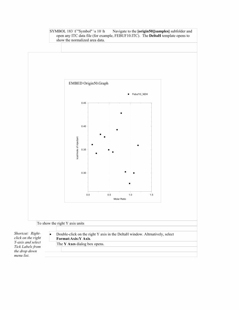
SYMBOL 183 \f "Symbol" \s 10 \h Navigate to the [origin50][samples] subfolder andopen any ITC data file (for example, FEBUF10.ITC). The DeltaH template opens toshow the normalized area data.
To show the right Y axis units
Double-click on the right Y axis in the DeltaH window. Altrnatively, selectFormat:Axis:Y Axis.The Y Axes dialog box opens.
Shortcut: Right-click on the rightY-axis and selectTick Labels fromthe drop downmenu list.
EMBED Origin50.Graph
0.0 0.5 1.0 1.5
0.30
0.35
0.40
0.45
Febuf10_NDH
Molar Ratio
kcal
/mol
e of
inje
ctan
t

Lesson 5: ITC Data Handling
Click on the Tick Labels Tab.
Select Right from the Selection List Box.
Click the Show Major Labels check box to insert a check mark.
Click OK.
The dialog box closes. The DeltaH window redraws to show tick labels along theright Y axis. The right axis labels are in units of calories/mole of injectant , while theleft axis labels are in kcal/mole of injectant.
EMBEDPBrush
EMBED Origin50.Graph
0.0 0.5 1.0 1.5
0.30
0.35
0.40
0.45
300
350
400
450
Febuf10_NDH
Molar Ratio
kcal
/mol
e of
inje
ctan
t

To factor the axis label values by 1000
Double-click on the right Y axis tick labels or select Format:Axis:Y Axis.The Y Axis dialog box opens.
Click on the Tick Labels Tab.
Select Right from the Selection List Box.
Enter 1000 in the Divide by Factor text box.
Click OK to close the dialog box.
Note : Now both axes plot in kcal since both are factored by 1000.
To save the changes into the DeltaH template file
Select File:SaveTemplate As….Origin opens a dialog box asking if you want to save the file as DELTAH.OTP (theDeltaH template file).
Click Cancel at this point if you do not want to change the original DeltaH template. Ifyou click OK, Origin will save the modified DeltaH window as DELTAH.OTP.
If you saved the modified template and now select the File:Read Data.. buttonthemodified DeltaH window will appear. Note that plotted data cannot be saved to atemplate file, so there is no need to delete the plotted area data before saving the DeltaHwindow.
To revert to the original DeltaH template
If you do decide to modify the DeltaH template, it is easy to recreate the original.Simply reverse the steps you used to create the modified template. That is, open theDeltaH window, open the Y-Axis dialog box, click on the Tick Labels tab, remove thecheck mark from the Show Major Labels check box, then select File: Save TemplateAs…
Modifying the RawITC template
The RawITC plot window shows bottom X axis tick labels in units of minutes. Let's usewhat we have just learned about factoring tick labels to change this axis scale so that thetick labels are in units of hours rather than minutes.
To factor the RawITC X axis tick labels by 3600
EMBEDPBrush
Shortcut:Click on the SaveTemplate icon fromthe Standardtoolbar.
EMBEDPBrus

Lesson 5: ITC Data Handling
Set the RawITC window as the active window (by either pressing and holding the Ctrlkey then pressing the Tab key, or selecting RawITC from the Window menu).
Double-click on the bottom X axis tick labels or select Format:Axis:X Axis.The X Axis dialog box opens.
Click on the Tick Labels Tab.
Select Bottom from the Selection List Box.
Enter 3600 in the Divide by Factor text box.Since the worksheet X values for raw ITC data are in terms of seconds, a factor of 3600gives us axis tick label values in units of hours for this axis.
Set Decimal Places to 2.
Click OK to close the dialog box.
Finally, double-click on the X axis title (it reads Time (min)) to open the Text Controldialog box, and edit the text to read Time (hrs).
To save the changes into the RawITC template file
Just as we did for the DeltaH template, select File: Save Template As.
Click Cancel in the Attention dialog box if you do not want to change the originalRawITC template. If you click OK, Origin will save the modified RawITC window asRawITC.OTP.
A Note About Units
Shortcut: Right-click on the bottomX-axis and selectTick Labels fromthe drop downmenu list

Raw data in ITC files are stored in terms of c al/second versus seconds, as you will seeif you open a worksheet containing raw data. The integrated area under the peaks dataare stored (in the worksheet column DH) in units of c al per injection. This is apparentif you open a worksheet containing integrated data.
However, for curve fitting and for better publication presentation, both the DeltaH andITCFinal plot windows present the integrated heat data as H' (kcal per mole of ligandinjected) which is more closely related to the fitting parameter H (calories per mole ofligand bound). That is, H' will be nearly equal to H (except for the factor of 1000) inearly injections when nearly all of the ligand added is bound. The factor of 1000 isachieved by entering that factor to the Y axis tick labels, as discussed earlier in thislesson.
Also, both the RawITC plot window and the upper graph in the ITCFinal plot windowdisplay X axis values in minutes, while the stored values are in seconds. In this case theX axis labels are factored by 60, as we discussed (for the RawITC window) earlier inthis lesson. If you double-click on the top X axis labels in the ITCFinal window, youwill notice there is a factor of 60 in the Divide by Factor text box , just as there was withthe RawITC window. Again, this factor setting is saved as part of the ITCFinaltemplate.
The Y axis data plotted in the DeltaH and lower ITCFinal templates (i.e., data with .ndhextension) are normalized on moles of injectant. If you ever wish to view theexperimental integrated heats in ca l per injection, then double-click on the Layer dialogbox, and move the _ndh file out of the Active data and move the _dh file into the Activedata. To complete the process, you must double-click on the Y axis tick labels andremove the factor of 1000.
include omega7 \* MERGEFORMAT Lesson 7: Advanced Curve Fitting
The model for one set of sites discussed in Lesson 1 will work for any number of sites nif all sites have the same K and H. If a macromolecule has sites with two differentvalues of K and/or H, then the model with two sets of sites must be used.
Whenever there are two sets of sites, the automatic initialization procedure is rarelyeffective. If the initialization parameters are extremely far away from best values, thenconvergence to the best values cannot take place as iterations proceed. In fact, often thefit gets worse rather than better with successive iterations. Therefore, the user must getinvolved in arriving at initialization parameters before the iterations can be started. Anindication of poor initialization occurs when values for the K parameter becomenegative during the fitting procedure.
Fitting with the Two Sets of Sites Model
The protein ovotransferrin has two very tight, non identical sites for binding ferric ions;one located in the N domain and one in the C domain. The Origin area dataFeOTF54.NDH shown below were obtained by titrating ovotransferrin with ferric ion.Injections 1-5 titrate primarily the stronger N site, injections 7-11 primarily the C site,while injections 13-15 result in no binding since both sites are already saturated.
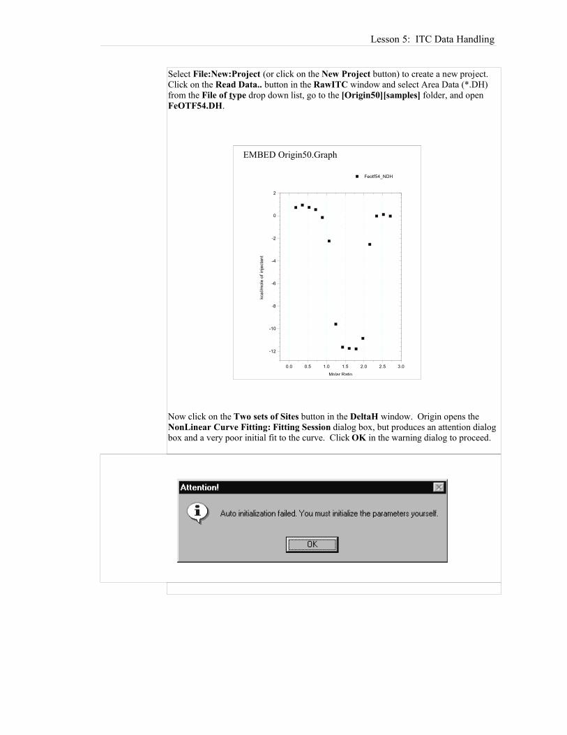
Lesson 5: ITC Data Handling
Select File:New:Project (or click on the New Project button) to create a new project.Click on the Read Data.. button in the RawITC window and select Area Data (*.DH)from the File of type drop down list, go to the [Origin50][samples] folder, and openFeOTF54.DH.
Now click on the Two sets of Sites button in the DeltaH window. Origin opens theNonLinear Curve Fitting: Fitting Session dialog box, but produces an attention dialogbox and a very poor initial fit to the curve. Click OK in the warning dialog to proceed.
EMBED Origin50.Graph
0.0 0.5 1.0 1.5 2.0 2.5 3.0
-12
-10
-8
-6
-4
-2
0
2
Feotf54_NDH
Molar Ratio
kcal
/mol
e of
inje
ctan
t

You will see that the auto initialization produces a curve which represents the data verypoorly. If iterations are started from this, the fit will not converge. A little intuition,however, will allow the operator to obtain a satisfactory initialization which will lead toconvergence.
Examination of the experimental points shows that the first few injections at a molar ratiobelow 1 produce ca. 1 kcal per mole of injectant, changing to ca. -12 kcal for molar ratio1 to 2 and finally changing to zero at molar ratios larger than 2. Begin manualinitialization then by entering 1 into both the N1 and N2 parameter boxes in the FittingSession dialog box. Because of the behavior noted above, H1 must be near +1000 andH2 close to -12,000, so enter these guesses into the appropriate parameter boxes. Sincethe experimental heats fall off quickly from the H1 value to the H2 value, it is clear thatK1 must be much larger than K2, and because the heat changes abruptly from the H2value to zero (i.e., beginning with the eleventh injection) it is also clear that K2 itselfmust be large (i.e., even though it is smaller than K1). Enter 1e8 into the K1 parameterbox, and 1e6 into the K2 parameter box. Be careful not to insert a space before or afterthe e when using exponential notation, or Origin will not accept the value.
Click on the Chi-Sqr button in the dialog box. Origin draws a new fit curve using theentered parameters, which is a much better representation of the data.

Lesson 5: ITC Data Handling
Though this fit is good enough to lead to correct convergence, we can still improve on itsome. Since the fit curve goes from H2 to zero much more gradually than the data, let'sincrease K2 from 1e6 to 1e8. We must still keep K1 larger than K2, so increase K1 from1e8 to 1e10. Click on Chi-Sqr button and observe that we now have a very goodinitialization curve. Select the 10 Iter. button a few times, and convergence occurs with afinal chi^2 of about 33,000.
Note that N1 and N2 are nearly the same magnitude, but not quite. It would beinteresting to see if a fit of nearly equal quality could be obtained with N1 and N2 exactlyequal to each other. (Although theoretically they should each be 1.0. Assign the value1.0 into the N1 and N2 parameter value box, click in the N1 and N2 checkboxes toremove the checkmark, and continue the iterations.
The final fit is not as good as when N1 and N2 are both floated, although there is noobvious explanation for this. Float all variables (by replacing the checkmark for N1 andN2) and iterate until you return to the earlier fit with a chi^2 of about 33,000. Note thatsometimes you may have to click on the 10 Iter. command many times before youachieve the smallest chi^2 value, as the fitting can become trapped in a local minimumfor several iterations. Click on the Done button to end the fitting session
NonLinear Least Squares Curve Fitting Session

Two NLSF Modes: Basic and AdvancedOrigin offers two modes of its nonlinear least squares fitter, Basic and Advanced. Whileboth modes allow you to fit your data, they differ substantilallly in the options theyprovide as well as in the degree of complexity.
By default, when you enter the NLSF Curve Fitting Session by selecting one of the threeITC curve fitting models, the Origin's nonlinear least squares fitter starts in the basicmode.
Basic ModeAllows for performing iterative curve fitting to the built in functions and plotting theresults to the graph. Click on the More… button to enter the Advanced mode.
Advanced ModeIn addition to the basic mode features the Advanced Mode allows for defining linearconstraints, adjusting the configuration of the fitting parameters, simulating data anddefining your own fitting function. Click on the Basic Mode button to return to theBasic mode.
Aborting the NLSF SessionIf you wish to exit the NLSF session without printing the fitting parameters to the Resultswindow or the graph text box, select the fitting session dialog box close EMBED PBrush
button and click No to the dialog box question: Do you want to end the current fittingsession?
Controlling the Fitting Procedure
You may enter the NLSF Curve Fitting Session and initialize the parameters by selectingone of the three fitting models (One Set of Sites, Two Sets of Sites or Sequential BindingSites). After the parameters have been determined you may re-enter the NLSF CurveFitting Session and keep the same fitting parameters by selecting from the menu, Math :Start Fitting Session. Normally the Fitter will open in the Basic mode, click on theMore… button to enter the Advanced Mode of the Fitter. From the Fitting Sessionwindow, select Options:Control to open the Control Parameters dialog box. Edit thisdialog box to specify several quantitative properties (as described below) of the fittingprocedure. These properties directly affect the way the fitter performs iterations.
The Control Parameters Dialog Box
For moreinformation on theFitting Session,press the F1 afteropening thedialog box.
EMBEDPBrush

Lesson 5: ITC Data Handling
The Tolerance Text BoxMicroCal has preset this value to be 0.05, but you may type a new value for the tolerancein this text box. When you click 'n Iter' in the Fit Session dialog box, this causes the fitterto try to perform, at most, n Levenberg-Marquardt (LM) iterations. If the relative changeof the value of chi-square between two successive iterations is less than the value in theTolerance text box, less than n iterations are performed. If you want the fitter to performstill more iterations, click on either the n Iter or the 1 Iter button in the Fitting Sessiondialog box. The value, 10, is specified as 'n' in the Max. Number of Iterations text box(see below).
The Max. Number of Iterations Drop-down ListSpecify the value for the maximum number of iterations performed when the n Iter buttonis clicked on in the Fitting Session dialog box. This has been preset by MicroCal to be10, but the user may change this number to be effective during a session of Origin, byentering a new value in the text box. However, the value will be reset to 10 after exitingOrigin.
The Derivative Delta GroupThis group determines how the fitter will compute the partial derivatives with respect toparameters for ITC fitting functions during the iterative procedure. If the Fixed Deltacheck box is unchecked (recommended for ITC users), then the actual value of Delta(derivative step size) for a particular parameter is equal to the current value of theparameter times the value specified in the Delta text box. The Maximum and Minimumtext boxes specify the limiting values of the actual Delta, in case a parameter valuebecomes too large or too small. MicroCal has preset the Delta to be .06 with the limitingmaximum to be 5 x 10+30 and the minimum to be 5 x 10-30. EMBED Equation.3 If
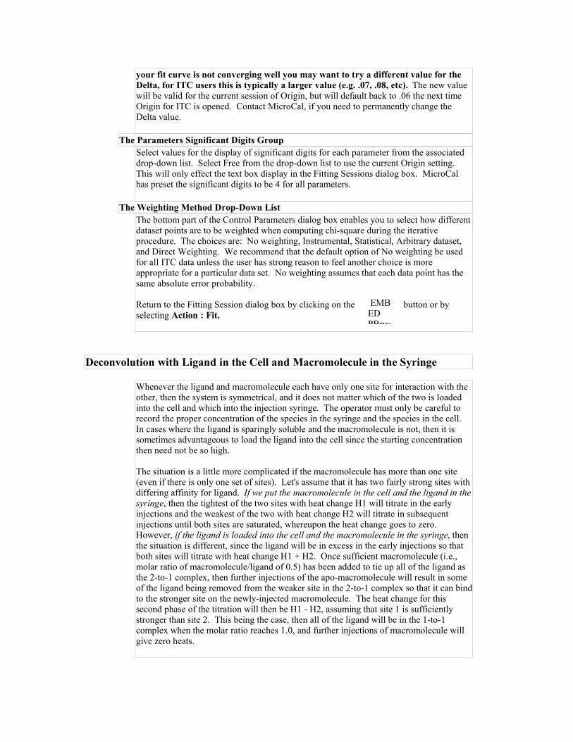
EMBEDPBrus
your fit curve is not converging well you may want to try a different value for theDelta, for ITC users this is typically a larger value (e.g. .07, .08, etc). The new valuewill be valid for the current session of Origin, but will default back to .06 the next timeOrigin for ITC is opened. Contact MicroCal, if you need to permanently change theDelta value.
The Parameters Significant Digits GroupSelect values for the display of significant digits for each parameter from the associateddrop-down list. Select Free from the drop-down list to use the current Origin setting.This will only effect the text box display in the Fitting Sessions dialog box. MicroCalhas preset the significant digits to be 4 for all parameters.
The Weighting Method Drop-Down ListThe bottom part of the Control Parameters dialog box enables you to select how differentdataset points are to be weighted when computing chi-square during the iterativeprocedure. The choices are: No weighting, Instrumental, Statistical, Arbitrary dataset,and Direct Weighting. We recommend that the default option of No weighting be usedfor all ITC data unless the user has strong reason to feel another choice is moreappropriate for a particular data set. No weighting assumes that each data point has thesame absolute error probability.
Return to the Fitting Session dialog box by clicking on the button or byselecting Action : Fit.
Deconvolution with Ligand in the Cell and Macromolecule in the Syringe
Whenever the ligand and macromolecule each have only one site for interaction with theother, then the system is symmetrical, and it does not matter which of the two is loadedinto the cell and which into the injection syringe. The operator must only be careful torecord the proper concentration of the species in the syringe and the species in the cell.In cases where the ligand is sparingly soluble and the macromolecule is not, then it issometimes advantageous to load the ligand into the cell since the starting concentrationthen need not be so high.
The situation is a little more complicated if the macromolecule has more than one site(even if there is only one set of sites). Let's assume that it has two fairly strong sites withdiffering affinity for ligand. If we put the macromolecule in the cell and the ligand in thesyringe, then the tightest of the two sites with heat change H1 will titrate in the earlyinjections and the weakest of the two with heat change H2 will titrate in subsequentinjections until both sites are saturated, whereupon the heat change goes to zero.However, if the ligand is loaded into the cell and the macromolecule in the syringe, thenthe situation is different, since the ligand will be in excess in the early injections so thatboth sites will titrate with heat change H1 + H2. Once sufficient macromolecule (i.e.,molar ratio of macromolecule/ligand of 0.5) has been added to tie up all of the ligand asthe 2-to-1 complex, then further injections of the apo-macromolecule will result in someof the ligand being removed from the weaker site in the 2-to-1 complex so that it can bindto the stronger site on the newly-injected macromolecule. The heat change for thissecond phase of the titration will then be H1 - H2, assuming that site 1 is sufficientlystronger than site 2. This being the case, then all of the ligand will be in the 1-to-1complex when the molar ratio reaches 1.0, and further injections of macromolecule willgive zero heats.

Lesson 5: ITC Data Handling
For example, take a look at the ITC integration data file OTFFe3.DH. To open this file,first click Done! in the fitting session menu bar to exit from the fitting session, then selectFile:New:Project (or click on the New Project button) to create a new project. Nowclick on the Read Data.. button in the RawITC window, select Files of type: Area Data(*.DH), then navigate to the [origin50][samples] folder, then double-click on OTFFe3in the File Name list. The normalized (.NDH) data plot into the plot window.
The data in file OTFFe3.DH were obtained with the macromolecule (ovotransferrin) inthe syringe and the ligand (a chelated form of ferric ion) in the cell. Injections 1-5correspond to formation of the diferric form of ovotransferrin with heat change H1 + H2.Injections 8-14 involve conversion of the diferric form into the mono ferric form withheat change H1 - H2.
Before fitting to this data, select Ligand is in (Cell) from the ITC menu.
Click OK in the Attention dialog box.
This switches the settings, letting Origin know that the ligand is now in the cell. Youmay confirm this by clicking on the ITC menu again and noting that the checkmark isnext to Ligand is in (Cell). (Note: Origin defines the "macromolecule" as the species
EMBED PBrush

with n greater than 1.0 and the "ligand" as the species with only one site, irrespective oftheir molecular weights.)
Now you can click on the Two Sets of Sites button to select the appropriate fittingmodel. The default fitting parameters will lead to a satisfactory convergence in this casebut lets try to improve on them before beginning interations. The first several injectionsindicate that H1 + H2 equals about -10,000 calories per mole. You might start off withvalues of -7000 for H1 and -3000 for H2. Set n1 and n2 equal to 1.0,, and click toremove the N1and N2 checkmark. Insert 1e8 for K1 and 1e6 for K2. Select Chi-Sqr,and use the 10 Iter. command to iterate until chi^2 no longer changes.
Notice that the estimated errors for K1 and K2 are quite large, being about 100% in thecase of K1. To verify this, change the K1 value from ca 3.2E7 to 5E7, remove thecheckmark from K1, and carry out 10 iterations. Remove the checkmark from K1 andclick on Chi-Sqr, which then shows a value of ca 32000. Click on 10 Iter. again, notethat the original K1 value of ca 3.2 x 10⁷ has reappeared, and that the new Chi-Sqr valueis only slightly smaller at ca 31000. Thus the two fits having very different fit parametervalues, have approximately the same Chi-Sqr. This is because these data show ratherlarge scatter from the smooth theoretical fit curve and are therefore not capable ofdefining precise values for the fitting parameters.
You may run across other instances in your own experiments when fitting parameters areeven more poorly defined than for OTFFe3.DH. The most likely situation for this tooccur is with two sets of sites, where K1 and K2 values are less than 10-fold different. Itis even possible that the set of "best fit" parameters may be quite different depending onthe initialization parameters which are used to start the fit; i.e., the curve-fitting routinecan become trapped in a local minimum for chi^2 and be unable to find the globalminimum. You can usually detect this by starting with several different sets ofinitialization parameters to see if you arrive at the same final minimum with nearly thesame fitting parameters.
When you are satisfied with the fit, click on the Done button in the dialog box to pastethe fitting parameters to the Results Window, the plot window and end the fittingsession. Go to the ITC menu, and reselect the default option, Ligand is in (Syringe)
EMBED PBrush

Lesson 5: ITC Data Handling
Deconvolution with the Sequential Binding Sites Model
All models discussed until now are concerned only with independent sites. It oftenoccurs in biological systems that the binding of a ligand to one site will be influenced bywhether or not ligands are bound to any of the other sites. If the sites happen to be non-identical in the first place, then binding studies alone cannot determine whether the sitesare independent or interacting. On the other hand, if the sites within a molecule areknown to be identical, then it is possible, sometimes, to determine if they are interacting.
Consider the simplest case, that of a macromolecule with two identical sites; this mightbe a homodimeric protein, for example. If the sites are identical, then we can no longerdistinguish between binding at the first site and binding at the second site, so thebookkeeping must be done in terms of the first ligand bound (K1, H1) and the secondligand bound (K2, H2), as described in the Appendix. A system with positivecooperativity means K2>K1, while negative cooperativity means K1>K2. Positivecooperativity is generally more difficult to distinguish from binding studies alone, sincethe tendency is for both sites on any single molecule to saturate together with heat changeH1 + H2, so that only one "phase" is seen in the titration curve. To determine ifcooperativity were present, one could use another technique which was able to show that,at half saturation, the dominant molecular forms were the macromolecule with either twoor no ligands attached, with very little of the singly-liganded form. Negativecooperativity can be more easily detected from binding studies, since there will be twodifferent "phases" occurring: the strong binding of the first ligand and the weakerbinding of the second.
The Origin file protb.dh shows integrated heat data on a macromolecule with twoidentical sites. If you have not done so yet click on Done! in the Fitting Sessionswindow to exit. Then select File:New:Project (or click on the New Project button) toopen a new project. To open protb.dh, click on the Read Data.. button in the RawITCwindow, then select Area Data (*.dh) from the File of Type: drop down box. Go to the[Origin50][samples] sub-folder, and double-click on protb.dh.
EMBED PBrush

Since there are clearly two phases to this binding isotherm, it exhibits negativecooperativity. Before fitting, edit the concentrations for this data as follows:
Click on the Concentration.. button in the DeltaH window.
Enter the following values in the dialog box: 20.7 mM ligand in the syringe; .494 mMmacromolecule in the cell; 4 l injection volume; 1.32 ml cell volume.
Click OK. Notice that the Y axis automatically rescales in accordance with the changesyou made.
Be sure to check the ITC menu to see that Ligand is in (Syringe) has the check mark ( ) next to it indicating it is the active mode. If the check mark is next to the Ligandis in (Cell), select the menu item Ligand is in (Syringe). This causes the mode to switchto having the ligand in the syringe.
To fit the data to the interacting sites model, click on the Sequential Binding Sitesbutton in the DeltaH window, then enter 2 for the number of sites. Enter guesses of 1e8,-8000, 1e6, -3000 for the parameters K1, H1, K2, and H2, respectively. Click on theChi-Sqr button to enter the above guesses then click on the 10 Iter. button several times,until you are satisfied with the convergence. These data can be deconvoluted with thedefault initialization parameters. The binding constant for the second ligand is about 70times weaker than for the first ligand, and the heat of binding is also less exothermic.Note that stoichiometric parameters n1 and n2 are not included as floating parameterswith the model of interacting sites, since this would allow a non-integral number ofligand molecules to bind in each step, which is a physical impossibility. This means thataccurate concentrations of ligand and macromolecule are more important here sinceconcentration errors cannot be covered up by non-integral values of n1 and n2 as is thecase with the model of two independent sites
(Note: Systems with identical binding sites have statistical degeneracy that influences thesaturation profile. For example, in a system with two identical sites the first ligand hastwo empty sites at which to bind while the second ligand has only one. The bindingconstants reported in the parameter box are phenomenological binding constants, whichinclude effects from degeneracy. To remove these effects and compare intrinisic bindingconstants Ko at each site, refer to eq (19) in the Appendix.
Binding of multiple ligands to transition metal ions
The binding of multiple ligands to transition metal ions is another example where thesequential binding model is appropriate, and where all sites are identical in the apo-metalion. The sample file Persson7.itc contains data on the binding of four Br- to Cd++ to

Lesson 5: ITC Data Handling
form CdBr4--. For practice call up the file and do curve fitting to obtain binding
parameters for each of the four bromide ions using the Sequential Binding Sites model.The concentrations of both Br- and Cd++ are correct as contained in the file.Convergence occurs (you must click on 10 Iter.. button several times) without operatorselection of initial parameters, but you may want to try to improve the initialization forpractice.
Using the Sequential Binding model with non-identical sites
The model of Sequential Binding can also be useful for systems with non-identical sites.The Two Sets of Sites model, discussed earlier, considers the saturation of individualsites on the same molecule, assumes they saturate independently of one another, and usesthree fitting parameters for each site; N, K and H. The model of Sequential Binding Sitesassumes a fixed sequence of binding, i.e., the first ligand which binds to an individualmolecule always binds to site 1, the second ligand which bids to an individual moleculealways binds to site 2, etc. The number of sequential sites must be exactly integral(1,2,3,…) so there is no fitting parameter equivalent to N, and best-fit is determined byonly two parameters, K and H, at each site once the total number of sites has beenselected by the operator. For a molecule which has 2 sites of quite different affinity (e.g.,K values different by a factor of five or more) the two models will tend to give equivalentvalues of K and H since thermodynamics will dictate binding to the site of highestaffinity first. However, when K values at two independent sites are more nearlyequivalent, then sequential binding will not be strictly followed.
EMBED Origin50.Graph
0 2 4 6 8 10 12
-0.5
0.0
0.5
1.0
1.5
Data: Persson7_NDH
Model: SequentialBindingSites
Chi^2 = 50.9854
K1 2332 ±35.68
H1 -320.6 ±6.428
S1 14.34
K2 117.0 ±5.193
H2 4525 ±121.6
S2 24.52
K3 2157 ±101.1
H3 1163 ±137.5
S3 19.12
K4 24.83 ±0.7786
H4 -6715 ±69.53
S4 -15.96
Persson7_NDH
Persson7_Fit
Molar Ratio
kcal
/mol
e o
f in
ject
ant

One inherent advantage of the sequential model is the smaller number of fittingparameters for each site. Using a model for independent sites, it would be extremelydifficult to obtain a unique fit for more than two sets of sites - which is why no fittingmodel for three sets of independent sites has been included in this software. As shownabove for the Persson7.itc file, the sequential model is capable of providing a unique fiteven for systems with four binding sites (if the K and/or H values are sufficientlydifferent for each site). Thus, for some multi-site systems the model of sequentialbinding may be the only choice available for providing a unique phenomenologicalcharacterization of binding parameters..
Simulating Curves
You may want to simulate titration experiments without actually going through the fittingroutine. The simulated curve may or may not be related to actual data which you haveobtained. To simulate data, there must be some ITC results in computer memory (eitherraw data called up, or an Origin project that contains data) but these results need not berelated to the simulations you carry out. The data in memory needs to contain at least asmany data points (or number of injections) as the curve you wish to simulate (Note: forproper simulation you must use a data file that had all injections of the same volume, sodo not use a file which used a preliminary 1st injection of a different size.)
To simulate a fit curve
Exit the fitting session and start a new project by selecting File:New:Project (or click onthe New Project button) from the menu. Click on the Read Data.. button in the RawITCwindow and select ITC Data (*.ITC) from the List Files As type box, and open theRnahhh.ITC data file located in the [Origin50][samples] folder (alternatively you mayread in the Area Data (*.dh) data file, Rnahhh.dh). The DeltaH window becomes theactive window.
Click on the Concentration.. button in the DeltaH window. When the concentrationsdialog box opens, change the concentrations and injection volume values to those desiredfor the simulation. For this example, set concentration in syringe to 14, concentration incell to 0.3, and injection volume to 3.0. (Note: If you do not see the Inject Vol. (ul) textbox, the file contained injections which were not all the same size, you will need to readin a different data file).

Lesson 5: ITC Data Handling
Click OK.
For this example we will simulate to the Two Sets of Sites model. Click on the Two setsof Sites button from the model fitting box. The Fitting Session dialog box will open withthe Two Sets of Sites model selected.
Enter the following parameters in the parameters text boxes:n1 = 1, K1 = 1e7, H1 = 10000, n2 = 1, K2 = 1e5, H2 = -10000.
Click on the Chi-Sqr button. The simulated curve yfit appears in the DeltaH window.Be careful not to click on the 1 or 10 Iter. buttons or the parameters will be changed.
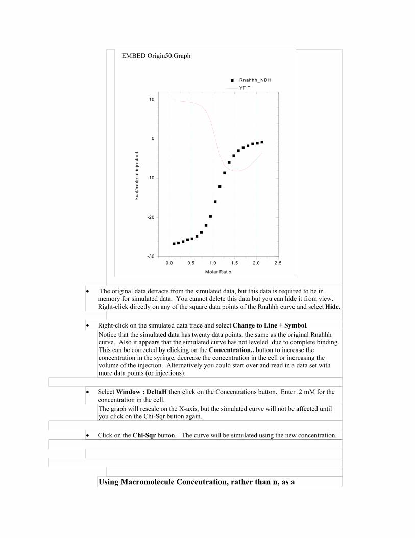
The original data detracts from the simulated data, but this data is required to be inmemory for simulated data. You cannot delete this data but you can hide it from view.Right-click directly on any of the square data points of the Rnahhh curve and select Hide.
Right-click on the simulated data trace and select Change to Line + Symbol.Notice that the simulated data has twenty data points, the same as the original Rnahhhcurve. Also it appears that the simulated curve has not leveled due to complete binding.This can be corrected by clicking on the Concentration.. button to increase theconcentration in the syringe, decrease the concentration in the cell or increasing thevolume of the injection. Alternatively you could start over and read in a data set withmore data points (or injections).
Select Window : DeltaH then click on the Concentrations button. Enter .2 mM for theconcentration in the cell.The graph will rescale on the X-axis, but the simulated curve will not be affected untilyou click on the Chi-Sqr button again.
Click on the Chi-Sqr button. The curve will be simulated using the new concentration.
Using Macromolecule Concentration, rather than n, as a
EMBED Origin50.Graph
0.0 0.5 1.0 1.5 2.0 2.5-30
-20
-10
0
10
Rnahhh_NDH
YFIT
Molar Ratio
kcal
/mol
e of
inje
ctan
t

Lesson 5: ITC Data Handling
Fitting Parameter
In some instances, you may know the value for the stoichiometric parameter n fromindependent studies, but are not able to come up with an accurate estimate formacromolecule concentration Mt (see Sigurskjold, Altman & Bundle, Eur. J. Biochem.197, 239-246 (1991). Using Origin, it is an easy matter to determine Mt (along with thecorrect binding constant and heat of binding) from curve-fitting. The procedure is asfollows: 1.) Guess at the macromolecular concentration and enter this incorrectconcentration, Mt*, into the Concentration dialog box. 2.) Select the model for curve-fitting and proceed to find the best fit in the usual way. The values which you obtain forthe binding constant and heat of binding will be correct since these depend only on theaccuracy of the ligand concentration. However, the best value which appears for thestochiometric parameter, n*, will be incorrect since you wish to assign this yourself and,after making the correct assignment n, to determine the actual Mt. 3.) Once curve-fittingis completed, you may calculate the correct Mt which is equal to the incorrectconcentration Mt* times the ratio n*/n. You may satisfy yourself that the aboveprocedure is correct by calling the RNAHHH.ITC data into Origin, do curve-fitting usingthe correct concentration, and record the best values of parameters n, K and H as thecorrect values. Now, change the concentration by multiplying the correct concentrationin the cell by 2 and enter that incorrect value into the Concentration dialog box. Docurve-fitting again and you will see that the new, incorrect value of n is exactly 50% ofthe correct value obtained using the correct concentration! The values for bindingconstant and heat of binding will be the same in the two cases.
include omega3 \* MERGEFORMAT Lesson 8: Other Useful Details
2 (chi-sqr) Minimization
The aim of the fitting procedure is to find those values of the parameters which bestdescribe the data. The standard way of defining the best fit is to choose the parametersso that the sum of the squares of the deviations of the theoretical curve(s) from theexperimental points for a range of independent variables is at a minimum. For the ITCmodels, where there is no weighting, the theoretical models can be represented by:
where: pi = the fitting parameters
the expression for 2 simplifies to :
where:
,...),,;( 321 pppxfy
221
2 ,...,;1 ppxfypn iieff

neff = the total number of experimental points used in the fitting
p = total number of adjustable parameters
yi = experimental data points
f(x;p1,p2,p3,…) = fitting function
Note: the difference d = neff - p is usually referred to as the number of degrees of freedom.
The above equation states that the Chi squared value of the fit is equal to the sum of thesquares of the deviations of the theoretical curve(s) from the experimental points dividedby the number of degrees of freedom. Since there is no weighting, it can be seen that thecalculated values are dependent on the magnitude of the scale and the number of datapoints.
Line Types for Fit Curves
You may select a line type to plot your data or fit curves from the Plot Details dialogbox. The Plot Details dialog box is available by double-clicking on the data plot, right-clicking on the data plot and selecting Plot Details from the shortcut menu or selectingthe desired data plot from the Data menu data list and selecting Format:Plot.
The Line Group
Select the desired line connection from the associated drop-down list. The lineconnection type affects interpolation results. The default line type for fit curves isStraight line. The most common method of connecting the fit curve data points arestraight, spline or B-spline:
Straight: A straight line is displayed between data points. This type of lineconnection will not give a smooth representation of the fit curve if there are few datapoints.
Spline: This option generates a cubic spline connection. To use the connection, the Xvalues must be discrete and increasing. Since curvature information is held in memory,the spline resolution remains the same regardless of page magnification. The SplineStepvariable in the ORIGIN.INI file controls the spline calculation increment. It is expressedin units of .1 point. This is usually the most satisfactory representation of the fit curve,but may exhibit an excursion from the actual fit curve if there is a sharp corner in thedata.
B-Spline: The B-spline curve can be described by parametric equations. Unlike splinecurves which pass through the original data points, the B-spline curve winds around theoriginal data points without passing through them. Thus this curve may not produce asatisfactory representation of the fit curve. For a complete discussion of the B-splineconnection, see the Origin User's Manual
Inserting an Origin graph into Microsoft® Word

Lesson 5: ITC Data Handling
There are two ways to include your Origin graph into Word (or other applications), youmay import your graph into Word or you may link (share) your graph with Word. Whenyou import your graph, Word will display the graph as an object and it cannot be editedby Origin tools (although it may be resized or reposition in the Word document). Whenyou link (share) your graph, Word displays the graph as an object which can be edited byOrigin and updated when the Origin graph changes.Please refer to the Origin manual for more information about Creating a GraphicPresentation.
Importing your graph into Word
Create you graph in Origin and when you are satisfied with its appearance, selectEdit:Copy page.
Open your Word document and click at the location where you want the graph to belocated.
Select Edit:Paste Special.
Select Origin Graph Object from the As list box.
Select the Paste radio button.
Click OK.
Linking your graph into Word
You must first create your graph in Origin and then save it as part of an Originproject (*.OPJ).
Open the saved Origin project (if it is not already opened) that includes the desiredgraph window.
Make the desired graph window active, select Edit:Copy Page.
Open your Word document and click at the location where you want to insert thegraph.
Select Edit:Paste Special.
Select Origin Graph Object from the As: list box
Select the Paste Link radio button.
Click OK.
After your Origin graph is linked to Word you may return to the original Origin graphand make changes to the graph. These changes can be reflected in the Word documentby:
Select Edit:Update Client from the Origin menu (to make immediate changes to theWord document graph).

(Shortcut: You may quickly start Origin and load the linked graph by simply double-clicking on the graph while in Word. Origin will be started with the original documentloaded, the changes can be made and by selecting Edit:Update Client, the changes willbe transferred to the Word document.)
Calculating a Mean Value for Reference Data
You may quickly calculate a mean value for the area data of any reference (or blank)injections by the following method. For this example we will calculate the mean of thearea data of the reference file Febuf10.itc (see Subtracting Reference Data starting onpage PAGEREF subtractingReference \h 32). From the RawITC window, click on Read Data.. button and open the file
Febuf10.itc (located in the [Origin50][Samples] folder).
Open the area data worksheet by right-clicking on any data point of the Febuf10.itcdata set in the DeltaH window and selecting Open Worksheet from the menu.
Select the NDH column by clicking on the column heading. All the cells of the column should be highlighted.
Click on the Statistics on Column(s) button. (Note: If you do not seethe button while the worksheet is open ; Select View:Toolbarsthen select the Worksheet check box.)
A new worksheet will appear with the mean, standard deviation, standard error of themean, the sum of the data and the number of data points of the NDH dataset column.
Appendix: Equations Used for Fitting ITC Binding Data
include omegandx \* MERGEFORMAT I. General Considerations
It will be assumed throughout that the macromolecule M is in the cell at an initial bulkconcentration Mto (moles/liter) before the first injection, and the ligand X to be injected isinitially at zero concentration in the cell. The working volume (cross-hatched area below) of thelollipop-shaped cell is Vo, the size of the ith injection is Vi and the total liquid which has beeninjected at any point during the experiment, V, is simply the sum of the individual V i for allinjections.
EMBEDPBrus
EMBED PBrush

Lesson 5: ITC Data Handling
Vo
V
At the beginning of an experiment, both the cell and the long communication tube are filled withmacromolecule solution, but it is only that contained within Vo that is sensed calorimetricallly,Because of the total-fill nature of the cell each injection acts to drive liquid out of the workingvolume and up into the inactive tube as shown by the darkened portion representing V. Thus,the concentration of macromolecule in V changes a small amount with each injection since thetotal number of moles of macromolecule initially in V (i.e. EMBED Unknown M t
o times Vo) atthe beginning of the experiment is later distributed in a larger volume, Vo + V . Since theaverage bulk concentration of macromolecule in V is the mean of the beginning concentrationEMBED Unknown M t
o and the present concentration Mt in the active volume, then conservationof mass requires that
EMBED Unknown M V M V M M Vto
o t o t to
12
(1)
so that
EMBED Unknown M M
VVV
V
t to o
o
12
12
(2)
Using similar reasoning, it is easily shown that the actual bulk concentration of ligand in Vo, Xt,is related to the hypothetical bulk concentration EMBED Unknown X t
o (assuming that all of theinjected ligand remained in Vo) as follows:
EMBED Unknown X V X V X Vto
o t o to
12
(3)
EMBED Unknown EMBED Unknown X X VVt t
o
o
1
2
(4)
The above expressions for Mt and Xt are used by Origin to correct for displaced volume effectswhich occur with each injection.
II. Single Set of Identical Sites

In the following equations,
K = Binding constant;n = # of sites;Vo = active cell volume;Mt and [M] are bulk and free concentration of macromolecule in Vo;Xt and [X] are bulk and free concentration of ligand, andEMBED Unknown = fraction of sites occupied by ligand X.
EMBED Unknown K
X
1 (5)
EMBED Unknown X X n Mt t (6)
Combining equations (5) and (6) above gives
EMBED Unknown 2 1 1 0
XnM nKM
XnM
t
t t
t
t
(7)
The total heat content Q of the solution contained in Vo (determined relative to zero for theunliganded species) at fractional saturation EMBED Unknown is
EMBED UnknownQ n M HVt o (8)
where H is the molar heat of ligand binding. Solving the quadratic equation (7) for EMBEDUnknown and then substituting this into eq. (8) gives
EMBED Unknown
QnM HVt o X
nM nKMX
nM nKMX
nMt
t t
t
t t
t
t
2
1 11 12 4
(9)
The value of Q above can be calculated (for any designated values of n, K, and H) at the endof the ith injection and designated Q(i). The parameter of interest for comparison withexperiment, however, is the change in heat content from the completion of the i-1 injection tocompletion of the i injection. The expression for Q in eq. (9) only applies to the liquid containedin volume Vo. Therefore, after completing an injection, it is obvious that a correction must bemade for displaced volume (i.e., Vi = injection volume) since some of the liquid in Vo after thei-1 injection will no longer be in Vo after the ith injection, even though it will contribute to theheat effect (assuming the kinetics of reaction and mixing are fast) before it passes out of theworking volume Vo. The liquid in the displaced volume contributes about 50% as much heat

Lesson 5: ITC Data Handling
effect as an equivalent volume remaining in Vo1 The correct expression then for heat released,
Q(i), from the ith injection is
EMBED Unknown
Q i Q i dVV
Q i Q i Q ii
o
( ) ( ) ( ) ( ) ( )
12
1 (10)
The process of fitting experimental data then involves 1) initial guesses (which most often canbe made accurately enough by Origin) of n, K, and H ; 2) calculation of Q (i) for eachinjection and comparison of these values with the measured heat for the correspondingexperimental injection; 3) improvement in the initial values of n, K, and H by standardMarquardt methods; and 4) iteration of the above procedure until no further significantimprovement in fit occurs with continued iteration.
III. Two Sets of Independent Sites
Using the same definition of symbols as above for set 1 and set 2, we have
EMBED Unknown K
X11
11
EMBED Unknown
K
X22
21
EMBED Unknown (11)
EMBED Unknown X X M n nt t 1 1 2 2 (12)
Solving equation (11) for EMBED Unknown 1 and EMBED Unknown 2 and thensubstituting into equation (12) gives
EMBED Unknown
X Xn M X K
X Kn M X K
X Ktt t
1 1
1
2 2
21 1(13)
Clearing equation (13) of fractions and collecting like terms leads to a cubic equation of theform
EMBED Unknown X p X q X r3 2 0 (14)
where
1 The first infinitesimal volume element in the i injection contributes no heat effect since it has alreadyequilibrated at existing concentrations after the i-1 injection. The last volume element of an injectioncontributes heat effects equal to the liquid remaining in Vo since its concentrations are equivalent to those inVo after the i injection. Assuming linearity over the small Vi volume increment, then the liquid in thedisplaced volume is only half as effective in producing heat relative to the liquid in Vo).

EMBED Unknown pK K
n n M Xt t 1 1
1 21 2
EMBED UnknownqnK
nK
MK K
XK Kt t
1
2
2
1 1 2 1 2
1 1 1
EMBED Unknownr XK K
t
1 2
(15)
Equations 14 and 15 can be solved for [X] either in closed form or (as done in Origin)numerically by using Newton’s Method if parameters n1, n2, K1, and K2 are assigned. Both 1
and 2 may then be obtained from equation 11 above.
As discussed earlier in section II, the heat content after any injection i is equal to
EMBED Unknown Q M V n H n Ht o 1 1 1 2 2 2 (16)
After a similar correction for displaced volume, the pertinent calculated heat effect for the iinjection is
EMBED UnknownQ i Q idVV
Q i Q i Q ii
o
( ) ( ) ( ) ( ) ( )
12
1
(17)
which may be used in the Marquardt algorithm to obtain best values for the six fittingparameters.
IV. Sequential Binding Sites
For sequential binding, the binding constants K1, K2, .....Kn must be defined relative to theprogress of saturation, so that
EMBED Unknown XM
MXK 1 EMBED Unknown
KMX
MX X22
EMBED Equation.2
(18)

Lesson 5: ITC Data Handling
In the sequential model, there is no distinction as to which sites are saturated, but only as to thetotal number of sites that are saturated. If the sites are identical, then there is a statisticaldegeneracy associated with the sequential saturation since the first ligand to bind has moreempty sites of the same kind to choose from than does the second ligand, etc. For identicalinteracting sites then, we can distinguish between the phenomenological binding constants Ki
(defined by eq (18)) and the intrinsic binding constants EMBED UnknownKio where the effect
of degeneracies has been removed. The relationship between the two binding constants is givenby:
EMBED Unknown oii K
iinK 1
(19)
All calculations given below, as well as parameters reported from curve-fitting, are in terms ofKi values but the operator may convert to EMBED Unknown Ki
o values, if desired, using eq(19). Since concentrations of all liganded species [MLi] can be easily expressed in terms of theconcentration of the non-liganded species, [M], then the fraction of total macromolecule having ibound ligands, Fi, is simply
EMBED Unknown FPo 1
EMBED Unknown FK X
P11
(20)
EMBED Unknown FK K X
P21 2
2
EMBED Unknown FK K K X
Pnn
n
1 2 ....
where
EMBED Unknown P K X K K X K K K Xnn 1 1 1 2
21 2[ ] [ ] .... .... [ ]
(21)
EMBED Unknown X X M iFt t ii
n
[ ]
1

Once n and values of fitting parameters K1 through Kn are assigned, then equations (20) - (21)may be solved for [X] by numerical methods (the Bisection method is used). After [X] isknown, all Fi may be calculated from equation (20) and the heat content after the ith injection isdetermined from
EMBED Unknown nnot HHHHFHHFHFVMQ ........... 32121211 (22)
And, as before,
EMBED UnknownQ i Q idVV
Q i Q i Q ii
o
( ) ( ) ( ) ( ) ( )
12
1
(23)
Which then leads into the Marquardt minimization routine.
Index INDEX \h "A" \c "2"
AAborting the NLSF Session, 58Active data set, 31, 37Active data set icon, 31Adjust integration session. see Integration detailsArea data. see also Subtracting reference (buffer) data
deleting, 34opening multiple runs, 27–29plotting in DeltaH window, 35–36saving, 10
ASCII data transfer. see Exporting ASCII data; Importing Worksheet dataAuto ITC Baseline command, 8Available Data list
in Layer Control dialog box, 29, 30, 35, 39in Math dialog box, 37, 38in Subtract Reference Data dialog box, 32
BBaseline
and Auto ITC Baseline command, 8creating automatically, 8modify in adjust integration session, 20–22
Binding equationsgeneral considerations, 73–74Sequential Binding Sites, 76–78

Lesson 5: ITC Data Handling
SingleSet of Identical Sites, 74–75Two Sets of Sites, 75–76
Blank injections. See Subtracting reference data
CCell Volume, 73Chi-Sqr button, 57, 64, 67, 68Chi-sqr Minimization, 69Control Parameters dialog box, 59–60Copy and paste worksheet data, 43–44Copy command, 43Curve fitting
fitting a straight line, 38invoking one of the three fitting models, 11line types, 69–70Nonlinear Least Squares Fitting Session, 11One Set of Sites, 11–12Sequential Binding Sites
fitting procedure, 63–66Two Sets of Sites, 55–60with ligand in cell and macromolecule in syringe, 63
DData
deleting, 34importing, 6
Data markersand setting integration range, 22
Data plotopening worksheet for, 44–46
Data Reader tool, 36Data set. see also ITC data
active, 37deleting, 34mean value, 71naming, 42naming conventions, 9, 41–42set as active, 31
Data, deleting points, 25Deconvolution. see Curve fittingDeleting bad data, 25DeltaH plot window. see templatesDerivative Delta Group, 59Draft view mode, 5, 19
EEditing concentration values, 10Exiting Origin, 18Exporting ASCII data, 44–46
FFinal figure, 15–17

Fitting Function dialog box, 11. see also Curve fittingFitting parameters
and Sequential Binding Sites, 63–66, 76–78and the single set of sites model, 11–12, 74–75and the two sets of sites model, 55–60, 75–76general considerations, 74text box, 12using macromolecule concentration, 68
IImporting data, 6Importing Worksheet Data, 47Initialization parameters, 55–58Installing Origin, 3Integrate injection peaks
in routine data analysis, 8Integrate on All Peaks command, 8, 23single peak, 22
Integration detailsand modifying baseline, 20–22defined, 19To adjust the integration range, 22, 21–23
ITC data. see also Subtracting reference (buffer) data; Area data; Routine ITC data analysisand opening multiple area data runs, 35–36and subtracting reference (buffer) data from reaction heat data, 27, 34–40data sets created in routine data analysis, 9, 41–42opening multiple area data runs, 27–29plotting in DeltaH window, 35–36
ITCFinal plot window. see TemplatesIterations
Max. Number of Iterations, 59
LLayer Contents list, 29, 30, 35, 39Layer Control dialog box, 29, 30, 35, 39Layer icon
double-clicking on, 29, 35, 39Line types for fit curves, 69–70Linear Regression command, 37
MMath dialog box
using to subtract reference data, 37, 38–39Mean value
of a data set, 71Menu Levels, 4
NNaming a data set, 9, 41–42
OOpening and Analyzing Previous Versions of Origin (*.ORG) Documents, 6

Lesson 5: ITC Data Handling
PPage view mode, 5, 19Paste command, 44Plot command, 42, 44Plot Details dialog box, 15–16, 23, 34, 42, 69Plot window templates. see TemplatesPlotting data. see Area data; ITC data; Raw ITC data files; Routine ITC data analysisPrint view mode, 5Project
opening, 19, 27, 35, 41saving, 18
RRaw ITC data files, opening, 7–8, 35, 41RawITC plot window. see TemplatesReaction heat, subtracting reference from. see ITC data; Subtracting reference (buffer) dataRead Data button, 6, 8, 49, 66Reference data. See Subtracting reference dataRegistering with MicroCal Software, 4Results window, 14Routine ITC data analysis. see also ITC data
and integrating injection peaks, 8and opening raw data files, 7–8, 35, 41
SSave area data, 10Sequential Binding Sites, 63–66
binding equations, 76–78multiple ligands to transition metal ions, 65non-identical sites, 65–66
Set Worksheet X command, 46Significant digits, 60Simple Math command, 37, 38Simulating Curves, 66–68Starting Origin, 4Subtract Reference Data button, 32Subtracting reference (buffer) data. see also ITC data
and calculating mean value for, 71and injection time spacing, 34, 39–40and opening multiple runs, 27–31subtracting a constant, 36–37subtracting a straight line, 37–39with a different number of injections than reaction data, 34–39
System requirements for Origin, 3
TTemplates
defined, 49DeltaH, 16, 19, 52ITCFinal, and creating a final figure for publication, 15–17modifying and saving, 49–52units used to display data in, 53–54
Text annotationsformatting, 12–14repositioning, 13
Tolerance Text Box, 59
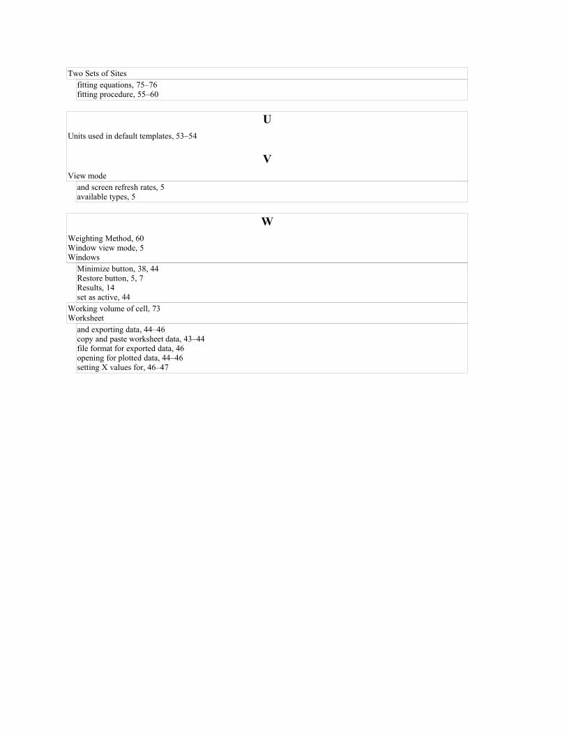
Two Sets of Sitesfitting equations, 75–76fitting procedure, 55–60
UUnits used in default templates, 53–54
VView mode
and screen refresh rates, 5available types, 5
WWeighting Method, 60Window view mode, 5Windows
Minimize button, 38, 44Restore button, 5, 7Results, 14set as active, 44
Working volume of cell, 73Worksheet
and exporting data, 44–46copy and paste worksheet data, 43–44file format for exported data, 46opening for plotted data, 44–46setting X values for, 46–47

Index