Embed Size (px)
Citation preview

January 2017
NASA/CR2017-219365
Tutorial for Collecting and Processing Images
of Composite Structures to Determine the Fiber
Volume Fraction
Lindsey Conklin
National Institute of Aerospace, Hampton, Virginia
https://ntrs.nasa.gov/search.jsp?R=20170001570 2018-06-28T21:55:37+00:00Z

NASA STI Program . . . in Profile
Since its founding, NASA has been dedicated to the advancement of aeronautics and space science. The NASA scientific and technical information (STI) program plays a key part in helping NASA maintain this important role.
The NASA STI program operates under the auspices of the Agency Chief Information Officer. It collects, organizes, provides for archiving, and disseminates NASA’s STI. The NASA STI program provides access to the NTRS Registered and its public interface, the NASA Technical Reports Server, thus providing one of the largest collections of aeronautical and space science STI in the world. Results are published in both non-NASA channels and by NASA in the NASA STI Report Series, which includes the following report types:
• TECHNICAL PUBLICATION. Reports of
completed research or a major significant phase of research that present the results of NASA Programs and include extensive data or theoretical analysis. Includes compilations of significant scientific and technical data and information deemed to be of continuing reference value. NASA counter-part of peer-reviewed formal professional papers but has less stringent limitations on manuscript length and extent of graphic presentations.
• TECHNICAL MEMORANDUM. Scientific and technical findings that are preliminary or of specialized interest, e.g., quick release reports, working papers, and bibliographies that contain minimal annotation. Does not contain extensive analysis.
• CONTRACTOR REPORT. Scientific and technical findings by NASA-sponsored contractors and grantees.
• CONFERENCE PUBLICATION. Collected papers from scientific and technical conferences, symposia, seminars, or other meetings sponsored or co-sponsored by NASA.
• SPECIAL PUBLICATION. Scientific, technical, or historical information from NASA programs, projects, and missions, often concerned with subjects having substantial public interest.
• TECHNICAL TRANSLATION. English-language translations of foreign scientific and technical material pertinent to NASA’s mission.
Specialized services also include organizing and publishing research results, distributing specialized research announcements and feeds, providing information desk and personal search support, and enabling data exchange services.
For more information about the NASA STI program, see the following:
• Access the NASA STI program home page at
http://www.sti.nasa.gov
• E-mail your question to [email protected]
• Phone the NASA STI Information Desk at 757-864-9658
• Write to: NASA STI Information Desk Mail Stop 148 NASA Langley Research Center Hampton, VA 23681-2199

National Aeronautics and
Space Administration
Langley Research Center Prepared for Langley Research Center
Hampton, Virginia 23681-2199 under Contract NNL09AA00A
January 2017
NASA/CR2017-219365
Tutorial for Collecting and Processing Images
of Composite Structures to Determine the Fiber
Volume Fraction
Lindsey Conklin
National Institute of Aerospace, Hampton, Virginia

Available from:
NASA STI Program / Mail Stop 148
NASA Langley Research Center
Hampton, VA 23681-2199
Fax: 757-864-6500
The use of trademarks or names of manufacturers in this report is for accurate reporting and does not
constitute an official endorsement, either expressed or implied, of such products or manufacturers by the
National Aeronautics and Space Administration.
iii
Table of Contents 1.0 Introduction ......................................................................................................................... 1 2.0 Collecting Images from the Microscope ............................................................................. 2 3.0 Image Processing Using ImageJ ....................................................................................... 12 4.0 Collecting Images of a Large Area of Interest .................................................................. 19 5.0 ImageJ Processing on Collected Noodle Images .............................................................. 33
List of Figures Figure 1. Covered microscope and computer. ................................................................................ 2
Figure 2. Microscope power switch. ............................................................................................... 2
Figure 3. Zeiss LSM 5 Exciter microscope. ................................................................................... 3
Figure 4. LSM, TV, and VIS buttons.............................................................................................. 3
Figure 5. Microscope touch screen. ................................................................................................ 4
Figure 6. Light source placed over area of interest. ........................................................................ 4
Figure 7. Microscope magnifications. ............................................................................................ 4
Figure 8. Course and fine adjustment knobs. .................................................................................. 5
Figure 9. Reflector settings. ............................................................................................................ 5
Figure 10. Computer desktop. ......................................................................................................... 5
Figure 11. Live button in AxioVision window. .............................................................................. 6
Figure 12. Live image in AxioVision window. .............................................................................. 6
Figure 13. Shading correction function. ......................................................................................... 7
Figure 14. MosaiX acquisition settings. ......................................................................................... 8
Figure 15. Results from autofocus error. ........................................................................................ 8
Figure 16. Full-scale image view. ................................................................................................... 9
Figure 17. MosaiX stitching function and results. .......................................................................... 9
Figure 18. Save As… window. ..................................................................................................... 10
Figure 19. Export window. ........................................................................................................... 11
Figure 20. Safely removing USB drive on desktop. ..................................................................... 11
Figure 21. Set Work position button. ............................................................................................ 12
Figure 22. Stage height confirmation............................................................................................ 12
Figure 23. ImageJ desktop icon. ................................................................................................... 13
Figure 24. ImageJ workspace. ...................................................................................................... 13
Figure 25. Opening a file in ImageJ.............................................................................................. 13
Figure 26. Selecting a file to open in ImageJ................................................................................ 13
Figure 27. RGB photometric interpretation. ................................................................................. 14
Figure 28. Control Panel. .............................................................................................................. 14
Figure 29. 8-bit image type selection. ........................................................................................... 14

iv
Figure 30. 8-bit photometric interpretation. .................................................................................. 14
Figure 31. ImageJ enhance contrast window. ............................................................................... 15
Figure 32. Example image (original). ........................................................................................... 15
Figure 33. Example image (after enhancing contrast). ................................................................. 15
Figure 34. ImageJ threshold window. ........................................................................................... 16
Figure 35. Example image (after auto-thresholding). ................................................................... 16
Figure 36. ImageJ Make Binary window. ..................................................................................... 16
Figure 37. Example image (after making binary). ........................................................................ 16
Figure 38. Sample image before opening. .................................................................................... 17
Figure 39. Sample image after opening. ....................................................................................... 17
Figure 40. Sample image before closing. ...................................................................................... 17
Figure 41. Sample image after closing. ........................................................................................ 17
Figure 42. Sample image before watershedding. .......................................................................... 17
Figure 43. Sample image after watershedding. ............................................................................ 17
Figure 44. ImageJ analyze particles window. ............................................................................... 18
Figure 45. Summary results from analyzing particles. ................................................................. 18
Figure 46. Example image (final result before analyzing particles). ............................................ 19
Figure 47. Alig. Rectangle tool. .................................................................................................... 19
Figure 49. Distance tool. ............................................................................................................... 20
Figure 50. Collected image to insert scale bar. ............................................................................. 21
Figure 51. Scale bar location in AxioVision window. .................................................................. 21
Figure 52. Scale bar placement on AxioVision window. ............................................................. 22
Figure 53. Scale bar’s automatic movement after exporting. ....................................................... 22
Figure 54. MosaiX Acquisition Setup window............................................................................. 23
Figure 55. Settings option in MosaiX Acquisition Setup window. .............................................. 23
Figure 56. Selected columns and rows in MosaiX Acquisition Setup window. ........................... 24
Figure 57. Current stage position relating to Setup grid. .............................................................. 24
Figure 58. Top image of noodle after stitching............................................................................. 25
Figure 59. Outlined area of interest. ............................................................................................. 25
Figure 60. Acquisition Setup tile for next image. ......................................................................... 26
Figure 61. Second collected image of noodle. .............................................................................. 26
Figure 62. Third – seventh collected images of noodle a) section 1, b) section 2, c) section 3, d)
section 4, and e) section 5. ................................................................................. 27
Figure 63. Panorama: Import from files option. ........................................................................... 28
Figure 65. Select folder with images for panorama. ..................................................................... 28
Figure 66. First image imported to make panorama. .................................................................... 29

v
Figure 67. First and second images imported to make panorama................................................. 29
Figure 68. Selection of tiles for deletion. ...................................................................................... 30
Figure 69. Selection second image for alignment. ........................................................................ 30
Figure 70. Second image alignment.............................................................................................. 31
Figure 71. Second image alignment, zoomed in. .......................................................................... 31
Figure 72. First and second noodle image combined in panorama workspace. ........................... 32
Figure 73. First and second noodle image combined in AxioVision workspace. .......................... 32
Figure 75. ImageJ Paintbrush tool location. ................................................................................. 33
Figure 76. ImageJ Brush Options for Paintbrush tool. ................................................................. 34
Figure 77. Traced scale bar of Figure 53 in ImageJ. .................................................................... 35
Figure 78. ImageJ Set Scale window. ........................................................................................... 35
Figure 79. Image dimension change to micrometers. ................................................................... 35
Figure 80. Global calibration warning message. .......................................................................... 36
Figure 81. ImageJ processing for complete noodle images. ......................................................... 36
Figure 82. ImageJ Wand (tracing) tool location. .......................................................................... 37
Figure 83. Noodle with yellow outline using tracing tool a) upper portion and b) lower portion.37
Figure 84. Threshold values set to 1 and 255. .............................................................................. 38
Figure 85. Entirely red thresholded noodle images a) upper portion and b) lower portion. ......... 38
Figure 86. Total area of the noodle. .............................................................................................. 39
Figure 87. Fiber area of the noodle. .............................................................................................. 39
Figure 88. Fiber Area Fraction Calculations Table. ..................................................................... 39

vi
Technology/Programs Used: Zeiss LSM 5 Exciter Microscope
AxioVision Release 4.8.2
ImageJ

1.0 Introduction
Fiber-reinforced composite structures have become more common in aerospace components due
to their light weight and structural efficiency. In general, the strength and stiffness of a composite
structure are directly related to the fiber volume fraction, which is defined as the fraction of fiber
volume to total volume of the composite. The most common method to measure the fiber volume
fraction is acid digestion, which is a useful method when the total weight of the composite and the
fiber weight can easily be obtained. However, acid digestion is a destructive test, so the material
will no longer be available for additional characterization. Acid digestion can also be difficult to
machine out specific components of a composite structure with complex geometries. These
disadvantages of acid digestion led the author to develop a method to calculate the fiber volume
fraction. The developed method uses optical microscopy to calculate the fiber area fraction based
on images of the cross section of the composite. The fiber area fraction and fiber volume fraction
are understood to be the same, based on the assumption that the shape and size of the fibers are
consistent in the depth of the composite. This tutorial explains the developed method for optically
determining fiber area fraction performed at NASA Langley Research Center.
The first step in the optical fiber-area-fraction determination is to section and polish a piece of the
composite structure in the area of interest. After polishing, the optical microscopy method uses a
confocal microscope, image collecting software, and image processing software. The confocal
microscope is a Zeiss LSM 5 Exciter 1microscope. The microscope has an automatic stage and
attached camera to easily collect images. The Zeiss image-collection software, AxioVision Release
4.8, is connected to the microscope. It can create stitched mosaics and panorama images of the
specimen underneath the microscope. After the images are collected from the microscope and
AxioVision, they are processed using the Java-based image-processing and analyzing software,
ImageJ.2 This software is open source, user-friendly, and has hundreds of plug-ins available to
users. After identifying the fibers in the image processing software, the fiber area fraction can be
calculated.
This tutorial first explains how to collect and process relatively small images. Then, a specific
example is used to describe how to collect and process images of complex structures. The complex
structure used in this example is a fluted-core sandwich structure that is comprised of facesheets,
webs, and noodles. The noodle specifically has complex geometry that would be difficult to
separate from the rest of the structure for acid digestion. Therefore, the developed optical method
is an ideal way of calculating the fiber volume fraction of this structural component.
1 is not an endorsement by the National Aeronautics and Space Administration 2 http://imagej.nih.gov/ij/

2
2.0 Collecting Images from the Microscope
1. Images can be collected using the Zeiss LSM 5 Exciter microscope (Fig. 1) currently
located in in Room 253 of Building 1205 at NASA Langley Research Center.
Figure 1. Covered microscope and computer.
2. Turn on the computer and the microscope.
a. The power switch is near the floor on a power strip on the left side of the
microscope (Fig. 2).
Figure 2. Microscope power switch.
b. The computer monitor also needs to be powered on. If the computer asks for a
password to log in under the username “administrator,” just press Enter on the
keyboard. A password is not required to log in.

3
3. Set up the microscope.
a. Take the blue cover off the microscope (Fig. 1). There are three buttons on the left
side of the microscope labeled LSM, TV, and VIS (Fig. 3). These buttons
represent the different viewing systems for the image. Press the VIS button in
order to see the image through the lens of the microscope (Fig. 4).
Figure 3. Zeiss LSM 5 Exciter microscope.
Figure 4. LSM, TV, and VIS buttons.
b. On the digital screen for the microscope settings, click Open for the RL-Shutter
(Fig. 5) in order to turn the light on. Then, manually move the specimen under the
microscope, so that the area of interest is under the light source (Fig. 6). Click on
Microscope in order to change to a different magnification. Starting at 5X, work
up to 100X (Fig. 7). Use the course and fine adjustment knobs (Fig. 8) in order to
focus on the specimen. These adjustment knobs are located on the right side of the
microscope, below the stage. Use the white joystick (Fig. 3) that is connected to
the microscope in order to look at a different area on the specimen. Note: If the
light does not appear to turn on, press on Reflector (next to Objectives at the top
White joystick
LSM, TV, VIS
buttons
Stage
Lens

4
of the screen). Then, click on BF, which stands for Brightfield (Fig. 9). This
should turn on the correct light.
Figure 5. Microscope touch screen.
Figure 6. Light source placed over area of interest.
Figure 7. Microscope magnifications.
Open shutter
Light source
100X magnification

5
Figure 8. Course and fine adjustment knobs.
Figure 9. Reflector settings.
4. Open AxioVision Rel. 4.8 on the computer desktop.
Figure 10. Computer desktop.
a. Instead of VIS, press the TV button on the left side of the microscope (Fig. 4).
This will allow the microscope image to be seen on the computer screen. Press the
Live button (Fig. 11) on the left hand side of the AxioVision window in order to
see the live image.
Course adjustment
(outer knob) Fine adjustment
(inner knob)
Brightfield reflector
AxioVision

6
Figure 11. Live button in AxioVision window.
b. In order to create the most optimal image, there are some options under the live
feed button (Fig. 12). Turn on the White Balance and Exposure options to
optimize the balance of color channels and adjust the exposure time, respectively.
Select the A. Min/Max and G. 0.45 (which is usually selected by default) in order
to optimize the contrast and brightness as well as the color reproduction on the
monitor, respectively.
Figure 12. Live image in AxioVision window.
5. Eliminate gradients that occur in the live image (Fig. 13).
a. Click on the Live Properties tab on the left hand side, underneath Live.
b. Click on the General tab.
c. Using the white joystick that is connected to the microscope, move the slide out
of the field of view (a.k.a. the specimen). For this specific type of specimen, move
to a region with uniform coloration. If there are any dust particles or anything that

7
would affect the shading, move the course adjustments to make the live image out
of focus.
d. Click on Shading Correction and wait for the system to calibrate. Note: If a
region with uniform coloration was properly selected, then this function will
correct any optical inhomogeneities. The ideal image will produce the same
colored pixels for all of the fiber cross-sections. This is optimally necessary for
thresholding in Step 17 of processing.
Figure 13. Shading correction function.
6. Create a stitched image of multiple microscope images.
a. Under the Work Area, click on MosaiX. Once it expands, click on Acquisition
(Fig. 14). Parameters and MosaiX settings will appear below.
b. Change the Autofocus from off to every tile (Fig. 14).
c. Note: If the resulting image looks like the image below (Fig. 15), then the amount
of rows chosen needs to be re-evaluated. If the camera starts to go beyond the
specimen area of interest, it will result in these unfocused areas towards the
bottom of the stitched image.

8
Figure 14. MosaiX acquisition settings.
Figure 15. Results from autofocus error.
d. Under the MosaiX settings, change the columns and rows as necessary. The
image needs to be less than 2000 MB (or 2 GB) in order to export it later. The
image size will display. Anything larger than a 29 X 29 image is not advised
because of 2GB memory limit of the computer. For this example, a 2 X 2 image
will be obtained (Fig. 14).
e. At the bottom of the acquisition settings (Fig. 14), press Start, and the
microscope camera will start capturing images and placing them together. This
may take up to an hour for a mosaic image that is relatively larger. For example, a
20 X 20 image will take a longer amount of time than a 10 X 10 image.
f. Note: If the captured images are all the same and the stage is not automatically
moving, then the program will need to be restarted. Cancel the current project and
exit out of AxioVision. Open AxioVision again and it should start working
properly.

9
g. To see the entire image, click on the magnifying glass with an arrow going
through it (Fig. 16).
Figure 16. Full-scale image view.
h. After the system has rendered multiple images, the images may not be correctly
aligned. In order to align images, click on Stitching, which is right below
Acquisition (Fig. 17). Do not change any parameters and press Start at the
bottom of the page (Fig. 17). The images should now be noticeably aligned. This
can be seen in the screenshot below (Fig. 17). As a result, the outer edges of the
entire image may be skewed. The alignment process is a much faster process than
the previous step of collecting all of the individual images.
Figure 17. MosaiX stitching function and results.
7. Save the project. File > Save As…
a. In order to save the project in AxioVision, save it as a .zvi file (the default file
type) (Fig. 18).

10
Figure 18. Save As… window.
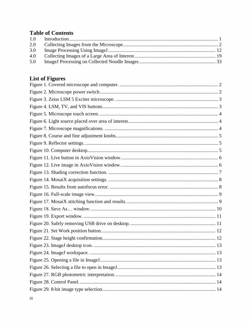
8. Export the stitched image. File > Export
a. Note: In order to save the image as high resolution, export the image as a .tif file
instead of saving as a .tif file.
b. Set the location for the exported file and set the File Type to TIF Tagged Image
File (Fig 19).
c. To save time and memory space, only export the stitched image. In order to do
this, all of the following choices need to be checked in the export menu (Fig. 19):
1. Generate merged image(s)
2. Merged images only
3. Gray scale
4. Convert to 8 bit
5. Apply display mappings
d. Click Start at the bottom of the window (Fig. 19). Remember that it will not
export an image that is above 2 GB. Under Output Files, the Status of the image
will say OK if the file was exported correctly. It will say Not enough memory
space if there is not enough memory on the computer or if the image is too large.
After the process is complete, verify that the file is in the designated location and
Close the export window.
11
Figure 19. Export window.
e. Note: If an error report message appears stating that AxioVision is going to close
after trying to export an image, follow these steps. In the Work Area, click on
Cameras > AxioCam MRc5. There will be three options: Adjust, Frame, and
General. Click on Frame and change the Camera Mode to B/W 1292 X 968
fast standard mode.
9. Copy the files onto a removable disk/USB drive.
a. Start > My Computer > Removable Disk
b. Drag the image files onto the Removable Disk Folder.
c. Once the files have been copied, safely remove the disk by clicking the icon on
the bottom-right of the desktop.
Figure 20. Safely removing USB drive on desktop.
10. Shut down the computer.
a. Exit AxioVision.
b. Start > Shut Down

12
c. Turn off the monitor.
11. Turn off the microscope.
a. On the digital touch screen, set the magnification to 5X (Fig. 7), and Close the
RL-Shutter (Fig. 7).
b. Click Load position (Fig. 7), then Set Work position (Fig. 21). A message
should appear stating Lower stage limit reached (Fig. 22). This means that the
stage is at the correct height for placement of subsequent specimens.
Figure 21. Set Work position button.
Figure 22. Stage height confirmation.
c. Turn the power off on the power strip and cover the microscope with the blue
cover.
3.0 Image Processing Using ImageJ
12. Download ImageJ using the following web address:
http://imagej.nih.gov/ij/download.html
13. Install ImageJ
14. Open/Run ImageJ. An illustration of the desktop image (Fig. 23) and the toolbar
workspace (Fig. 24) are provided below.

13
Figure 23. ImageJ desktop icon.
Figure 24. ImageJ workspace.
15. Open a file in ImageJ using File > Open (Fig. 25).
Figure 25. Opening a file in ImageJ.
a. Select the image to be used in processing (Fig. 26).
Figure 26. Selecting a file to open in ImageJ.
b. Ensure the photometric interpretation of the image is 8-bit and not RGB. This
information can be found directly above the displayed image. If the image is RGB
(Fig. 27), right click the image and select Control Panel (Fig. 28). Expand the
Image option, expand Type and select 8-bit (Fig. 29). Then, exit out of that
window. The description should now say 8-bit above the image (Fig. 30).

14
Figure 27. RGB photometric interpretation.
Figure 28. Control Panel. Figure 29. 8-bit image type selection.
Figure 30. 8-bit photometric interpretation.
16. Process > Enhance Contrast
a. Set the Saturated Pixels to 20% for high contrast. This setting can be changed
depending on how much contrast is needed. Also, check the box that says
Normalize (Fig. 31). The image before enhancing contrast (Fig. 32) and the
image after enhancing contrast (Fig. 33) are below.

15
Figure 31. ImageJ enhance contrast window.
Figure 32. Example image (original). Figure 33. Example image (after
enhancing contrast).
17. Image > Adjust > Threshold (Ctrl+Shift+T)
a. The threshold will usually select the red background; however, the opposite is
needed. In order to threshold (select in red) the fiber cross sections, check the box
that says Dark background (Fig. 34). This will invert the threshold selection
(Fig. 35).
b. Note: The threshold value bars are automatically set to default. It is recommended
not to change these. If the bars need to be adjusted, then the region of uniform
coloration (Step 5(c)) was incorrectly selected. This problem indicates that optical
inhomogeneities are present in the image. The fiber cross sections should ideally
be the same color, so the processor can automatically select all fiber cross section
pixels.

16
Figure 34. ImageJ threshold window. Figure 35. Example image (after auto-
thresholding).
18. Process > Smooth
19. Process > Binary > Make Binary
a. Keep all of the boxes checked and press OK (Fig. 36).
Figure 36. ImageJ Make Binary window. Figure 37. Example image (after making
binary).
20. Process > Binary > Open
a. Use this option if there are unnecessary and isolated pixels that are artifacts of the
image collection process. For example, see the images below (Figs. 38 and 39):
Threshold bars

17
Figure 38. Sample image before opening. Figure 39. Sample image after opening.
b. This will remove isolated pixels that appear in the binary image.
21. Process > Binary > Close
a. Use this option if holes need to be filled in various regions. For example, see the
images below (Figs. 40 and 41):
Figure 40. Sample image before closing. Figure 41. Sample image after closing.
b. This process will fill small holes that appear in the binary image.
c. Note: Sometimes, this option will merge 45 cross-sections together because it
will eliminate the small gaps in between them. This should not happen! Click
Edit > Undo in order to undo this process.
22. Process > Binary > Watershed
a. After completing Step 21, the fiber cross sections might be touching/overlapping
in the binary image. The watershed option (Figs. 42 and 43) uses segmentation to
separate the cross sections from one another. It works best when the objects are
not significantly overlapped.
Figure 42. Sample image before
watershedding.
Figure 43. Sample image after
watershedding.
b. This step takes a while for the larger images.
23. Is there unwanted area that should not be in the fiber-volume-fraction calculation?

18
a. Use the polygon selection tool in order to isolate the desired area directly
before analyzing the particles in Step 24. Outline each part that is to be included
with a left click and end the shape with a right click. Then, it will calculate the
area of the cross-section in the selected area.
24. Analyze > Analyze Particles
a. Only check the box (Fig. 44) that is labeled:
1. Summarize
b. Then, click OK (Fig. 44).
Figure 44. ImageJ analyze particles window.
c. A window will open that is labeled as the Summary (Fig. 45) of the final image
(Fig. 46). The most important categories for fiber-volume-fraction measurement
are Total Area and % Area (Fig. 45). Note: The Total Area represents the fiber
cross-sectional area (not the total area of the selected area) and the % Area
represents the percentage of fiber cross sections compared to the total area in the
selected space. Dividing the Total Area by the % Area (once turned into a
decimal) will give the area of the entire selected area.
Figure 45. Summary results from analyzing particles.

19
Figure 46. Example image (result before analyzing particles).
4.0 Collecting Images of a Large Area of Interest
Here are tips on how to use the microscope to collect images of a large area of interest, such as a
unidirectional carbon fiber noodle.
25. Obtain a 5X image of the entire noodle to find measurements.
a. Change the magnification of the microscope to 5X (Fig. 7).
b. Make a 3 X 3 or 4 X 4 image in order to create a mosaic of the entire noodle.
c. The noodle needs to be split into two halves because of the 2 GB memory
restrictions on the computer. Use the Alig. Rectangle tool (Fig. 47) in order to
create an outline for the top and bottom halves (Fig. 48). It will create red
rectangles around the selection and post the area for that square in µm2 (Fig. 48).
Figure 47. Alig. Rectangle tool.

20
Figure 48. Noodle measurements (3 X 3 image, 5X magnification).
d. Now that the rectangles have been created, use the Distance tool (Fig. 49) to find
the length and width for each rectangle (Fig. 48).
Figure 49. Distance tool.
e. Save or export the image in order to use this as a reference for deciding how many
columns and rows the image needs to be in Step 26(de). Exporting the image
will additionally require checking the box that says Burn in Annotations in the
export window (Fig. 19). This will permanently put the measurements on the
image. Notice that the top rectangle (Fig. 48) has dimensions of 5501.79 µm
(horizontal distance) X 1234.79 µm (vertical distance). The final image should
look similar to figure 48.
26. Create a small 100X image that includes a scale bar.
a. Change the magnification of the microscope on the microscope’s touch screen
from 5X to 100X (Fig. 7).
b. Under MosaiX > Acquisition, create a 3 X 3 image of any part of the specimen
that is outside of the noodle area. A white scale bar will be easier to view without
the fiber cross sections in sight. (Fig. 50).

21
Figure 50. Collected image to insert scale bar.
c. Click on the scale bar on the far left side of the AxioVision window (Fig. 51).
Click on the top-left of the 3 X 3 image and hold down the click. Drag a line
towards the top-right corner of the 3 X 3 image (Fig. 52). Drag the line far enough
to make a 100 µm scale bar.
Figure 51. Scale bar location in AxioVision window.
Scale bar

22
Figure 52. Scale bar placement on AxioVision window.
d. Export the image with the same options found in Step 8 (Fig. 19). Additionally,
click on Burn in Annotations in order to keep the scale bar in the exported
image. Note: Verify that the image was exported to the correct location. After the
image file was opened, note that the scale bar has moved toward the bottom-right
of the image (Fig. 53). This is why the placement of the scale bar (Fig. 52) in Step
26(c) is important.
Figure 53. Scale bar’s automatic movement after exporting.
e. Copy this image onto a flash drive in order to be used in Step 34.
27. Setting up the mosaic image to make the first (or top) half of entire area of interest.
a. Under MosaiX > Acquisition, click on Setup… under MosaiX Settings. A
window will appear that looks similar to the image below (Fig. 54).

23
Figure 54. MosaiX Acquisition Setup window.
b. Use the white joystick connected to the computer (Fig. 3) and coarse and fine
adjustments (Fig. 3) to move the specimen to the starting point of the top half.
The live stage image can be seen below the settings (Fig. 54). The starting point
will be the top-left corner of the first image.
c. Click on the Settings tab (Fig 55).
Figure 55. Settings option in MosaiX Acquisition Setup window.
d. Start to increase the number of columns until the top number of the MosaiX size
(µm) is slightly larger than the horizontal distance found in the top rectangle (Fig.
49). The example uses 42 columns because the corresponding MosaiX size of
5553.94 µm (Fig. 56) is slightly larger than the distance of 5501.79 µm (Fig. 49).
e. Start to increase the number of rows until the bottom number of the MosaiX size
(µm) is slightly larger than the vertical distance for the top half. The example uses
13 rows because the corresponding MosaiX size of 1274.17 µm (Fig. 56) is
slightly larger than the distance of 1234.79 µm (Fig. 49).
Live stage
image
Settings
Blue grid

24
Figure 56. Selected columns and rows in MosaiX Acquisition Setup window.
f. In the grid that is created on the right of the settings window (Fig. 57), there is a
blue grid that contains the selected number of rows and columns with a green plus
sign in the middle. The plus sign represents where the current stage position is
located. The current stage position needs to be placed at the top-left corner of the
grid. In order to do this, press the button that looks like a square with a green
plus sign on the top-left corner . After hovering over the icon, a text box will
appear stating “Moves the MosaiX image to the current stage position.” The
icon is located below the grid space in the row of options. Note: Every time the
stage position is moved to the desired starting point, this button needs to be
selected again. The stage position can only be selected on the grid, but the current
live image can be seen under the settings.
Figure 57. Current stage position relating to Setup grid.
g. Select the OK button at the bottom-right of the window (Fig. 57). Then, select
Start in the MosaiX Acquisition to start creating the image. It may require a few
trials to find the correct starting point and number of rows and columns.
Blue grid
Green plus sign
Current stage
position

25
h. Stitch together the image, which is the option below Acquisition for MosaiX.
The final result should look like the image below (Fig. 58):
Figure 58. Top image of noodle after stitching.
28. Setting up the mosaic images to make the second (or bottom) half.
a. Now that the top image has been created, the image will be used as a guide to
acquire the next set of images. First, identify the individual tiles that make up the
entire image. In the last row of the image below, identify the two outermost tiles
of the area of interest (Fig. 59).
Figure 59. Outlined area of interest.
b. These identified tiles (Fig. 59) represent the bounding tiles for the top of the next
image to be collected. These tiles are both seven tiles in from the left and right
side, so a total of 14 tiles should be deleted from the original number of columns.
Therefore, the next image should have 28 columns.
c. In the MosaiX > Acquisition > Setup > Settings, the live image needs to be
moved to the next starting point. In order to do this, double click on the tile that
was marked by the left arrow in the image above. The green plus sign should now
be in the newly identified tile (Fig. 60). Note: By using this tile as a starting point,
the initial tile will collect a row of tiles already collected in the previous image.
This is necessary in order for the images to overlap and align later.

26
Figure 60. Acquisition Setup tile for next image.
d. Press the button that looks like a square with a green plus sign on the top-left
corner . Hovering over the icon will cause it to say “Moves the MosaiX
image to the current stage position.” It is located below the grid space in the
row of options (Fig. 57). This will make that specific tile the top left corner of the
new image.
e. Change the number of columns according to the explanation in Step 28(b).
Change the number of rows as required, remaining in the field of view. The next
image in this example is a 28 X 5 mosaic (Fig. 61).
Figure 61. Second collected image of noodle.
f. Continue Steps 28(a–e) until images have been collected of the entire noodle
(Fig. 62). After collecting each one, stitch each respective image together. Save
each image as a .zvi file. When choosing names for these files, include numbers
so that the order of image collection is easily identifiable. Finally, save all of the
files into one folder to make them easier to access later. See the images below that
were created to form the whole noodle.

27
Figure 62. Third – seventh collected images of noodle a) section 1, b) section 2, c) section 3, d)
section 4, and e) section 5.
29. Stitch the images together using Panorama > Import from Files.
a. Above the MosaiX option is the Panorama option. Once expanded in the menu,
choose the second option: Import from Files (Fig. 63).
(a)
(b)
(c)
(d)
(e)

28
Figure 63. Panorama: Import from files option.
b. Click the button with three dots in the top-left of the window (Fig. 64) in
order to open the folder that includes all of the .zvi files. The folders will start to
open below (Fig. 65).
Figure 64. Open files to be imported for panorama.
Figure 65. Select folder with images for panorama.
c. Select the first image that was collected in Step 27. The image should appear in
the workspace to the right (Fig. 66).

29
Figure 66. First image imported to make panorama.
d. Select the second image that was collected in Step 27. The second image usually
does not appear in the immediate field of view, so scroll down or across to find
the second image in the workspace (Fig. 67).
Figure 67. First and second images imported to make panorama.
e. Delete any unnecessary tiles that are not a part of the area of interest. Hold down
the Ctrl button as tiles are selected to be deleted (Fig. 68). Then, click on the
button with green tiles and a red X (Fig. 68) that is located at the bottom of the
page. This will delete the selected tiles.
First imported
image
Second imported
image

30
Figure 68. Selection of tiles for deletion.
f. To move the second set of image tiles, hold down the Ctrl button and select each
individual tile of the second image (Fig. 69). Do not move the tiles as they are
being selected. If the tiles accidently move while being selected, press Ctrl + z to
undo.
Figure 69. Selection second image for alignment.
g. After all of the tiles are selected, move the collection of images towards the first
image by clicking a part of the selected collection and dragging it towards the first
set of images (Fig. 70). Align the images on top of each other by zooming in and
watching the bottom of the first image collection overlap with the top of the
second image collection (Fig. 71). This is why the previous note in Step 28(c) of
overlapping the image collections is very important.
Selected
tiles to be
deleted

31
Figure 70. Second image alignment.
Figure 71. Second image alignment, zoomed in.
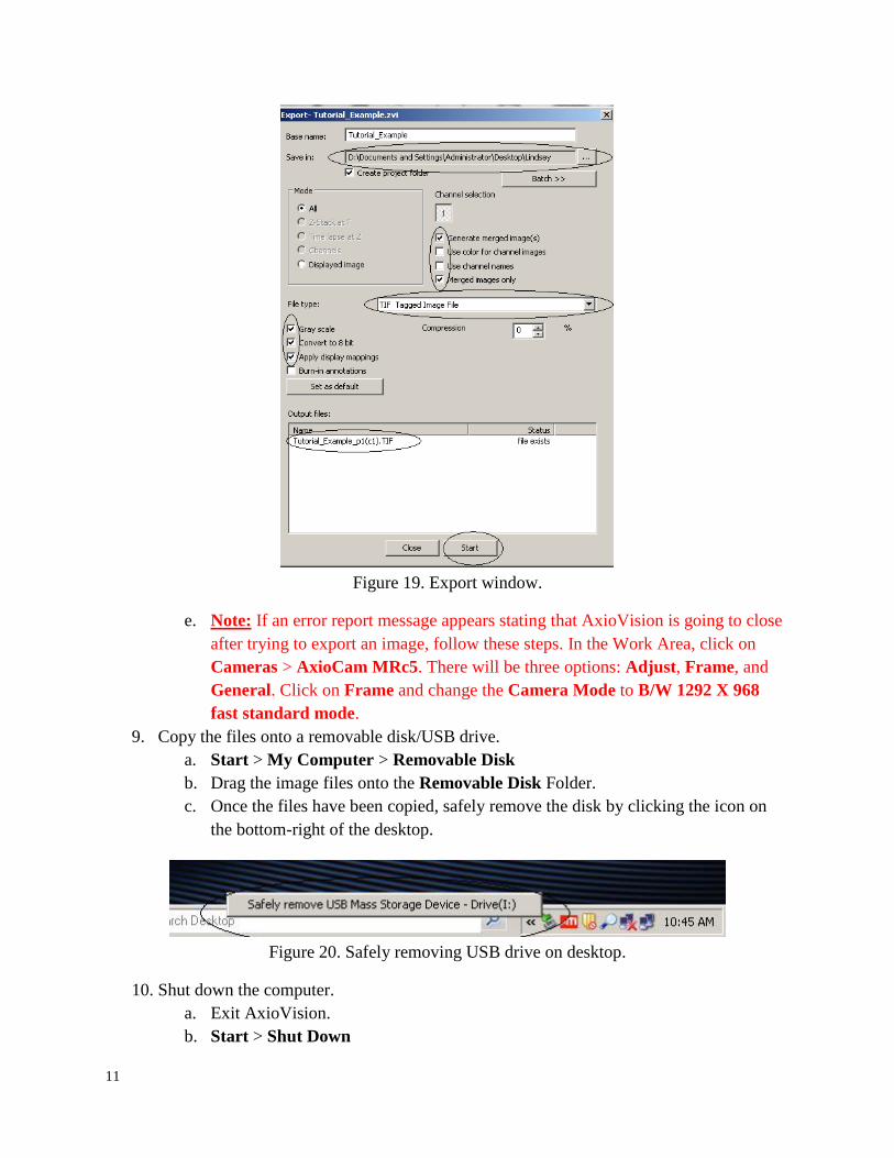
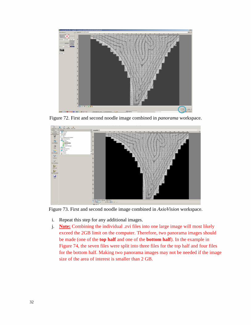
h. Press OK at the bottom-right of the panorama workspace (Fig. 72). The image
should now appear in a .zvi file format in the AxioVision workspace (Fig. 73).
Export the panorama image as a .tif file. Place it on a removable disk or flash
drive.
32
Figure 72. First and second noodle image combined in panorama workspace.
Figure 73. First and second noodle image combined in AxioVision workspace.
i. Repeat this step for any additional images.
j. Note: Combining the individual .zvi files into one large image will most likely
exceed the 2GB limit on the computer. Therefore, two panorama images should
be made (one of the top half and one of the bottom half). In the example in
Figure 74, the seven files were split into three files for the top half and four files
for the bottom half. Making two panorama images may not be needed if the image
size of the area of interest is smaller than 2 GB.

33
(a)
(b)
Figure 74. Outlined noodle using ImageJ Paintbrush tool a) upper portion and b) lower portion.
5.0 ImageJ Processing on Collected Noodle Images
30. After opening ImageJ, open the two images that were created in Step 29.
31. Double-click on the Paintbrush Tool in the tool bar (Fig. 75). The Brush Options
window will appear.
Figure 75. ImageJ Paintbrush tool location.
a. Manually change the Brush width to 100 (Fig 76).
b. Change the Color to Black (Fig. 76).

34
Figure 76. ImageJ Brush Options for Paintbrush tool.
32. Outline and define the fibers that are part of the area of interest.
a. Use the Paintbrush Tool in order to eliminate what is not a part of the area of
interest.
b. Note: Use the Magnifying Glass tool to zoom in and out with the
Paintbrush Tool and clearly define/outline the area of interest.
c. Color in the rest of the unnecessary parts using a Brush width of 200.
d. The final results should look like the two images shown before (Fig. 74a and Fig.
74b).
33. Eliminate the overlapping between the two images.
a. Use the Paintbrush Tool to make a straight line across the bottom of the first
image and the top of the second image. Hold down Shift while using the tool in
order to make straight horizontal lines.
b. This might take a few trial and error sessions to ensure that the correct amount of
the overlapping noodle was removed.
c. Note: Save these individual images (Fig. 74) in order to find the total area of the
noodle later.
34. Set the measurement scale from pixels to µm.
a. Open up the image created with a scale bar in Step 26 (Fig. 53).
b. Use the Straight Line Selection Tool in order to trace the known distance
(Fig. 77).

35
Figure 77. Traced scale bar of Figure 53 in ImageJ.
c. Analyze > Set Scale…
d. Enter in the Known distance (Fig. 78), which is 100 µm.
e. Change the Unit of length to “micrometers” (Fig. 78).
f. Check the box that says Global (Fig. 78) in order to apply this to all images that
will be manipulated.
g. Press OK (Fig. 78).
Figure 78. ImageJ Set Scale window.
h. Now, at the top left of the current image, the dimensions should display # X #
micrometers (Fig 79).
Figure 79. Image dimension change to micrometers.

36
i. Note: After applying this scaling, and choosing to open a new image, a message
may appear that looks like the image in Fig. 80. Exit out of the window in order to
keep the same scaling.
Figure 80. Global calibration warning message.
35. Perform Steps 16–23 in order to complete the image processing.
a. Save the processed images (Fig. 81) as different files than the previous images
(Fig. 76).
Figure 81. ImageJ processing for complete noodle images.
36. Determine the total area of the noodle.
a. Open the outlined images (Fig. 76) in ImageJ.

37
b. Use the Wand (tracing) tool (Fig. 82) in order to select the entire noodle
area. This is best done by clicking on any part of the black portion outlining the
noodle. Successful outlining can be seen when the entire area of interest has a
yellow outline (Fig 83).
Figure 82. ImageJ Wand (tracing) tool location.
Figure 83. Noodle with yellow outline using tracing tool a) upper portion and b) lower portion.
c. Image > Adjust > Threshold… Change the minimum threshold value to 1 and
the maximum threshold value to 255 (Fig. 84). The area of interest should be
entirely red (Fig. 85).
(a)
(b)

38
Figure 84. Threshold values set to 1 and 255.
Figure 85. Entirely red thresholded noodle images a) upper portion and b) lower portion.
d. Analyze > Analyze Particles… Add the total areas calculated by this function
(Fig. 86). These two numbers are the only numbers needed from this step. Note:
If the calculated areas in the summary table are close to zero or do not look
correct, then redo the function after getting rid of the yellow outlines of the
noodle. Note that the red thresholding should still be there.
(a)
(b)

39
Figure 86. Total area of the noodle.
37. Determine the area of fibers inside the noodle.
a. Open the processed images (Fig. 81).
b. Analyze > Analyze Particles… Add the total areas calculated by this function
(Fig. 87). This will represent the total amount of fiber area inside the noodle.
Figure 87. Fiber area of the noodle.
38. Determine the fiber area fraction based on the numbers calculated in Steps 36 and 37
(Figs. 86 and 87).
Noodle Part Fiber Area Total Area Fiber Area Fraction
Top Half 2.76 mm2 5.01 mm2 0.5509
Bottom Half 1.16 mm2 2.21 mm2 0.5249
Total Noodle 3.92 mm2 7.22 mm2 0.5429
Figure 88. Fiber Area Fraction Calculations Table.

REPORT DOCUMENTATION PAGE
Standard Form 298 (Rev. 8/98) Prescribed by ANSI Std. Z39.18
Form Approved OMB No. 0704-0188
The public reporting burden for this collection of information is estimated to average 1 hour per response, including the time for reviewing instructions, searching existing datasources, gathering and maintaining the data needed, and completing and reviewing the collection of information. Send comments regarding this burden estimate or any otheraspect of this collection of information, including suggestions for reducing the burden, to Department of Defense, Washington Headquarters Services, Directorate for InformationOperations and Reports (0704-0188), 1215 Jefferson Davis Highway, Suite 1204, Arlington, VA 22202-4302. Respondents should be aware that notwithstanding any otherprovision of law, no person shall be subject to any penalty for failing to comply with a collection of information if it does not display a currently valid OMB control number. PLEASE DO NOT RETURN YOUR FORM TO THE ABOVE ADDRESS.
1. REPORT DATE (DD-MM-YYYY) 2. REPORT TYPE 3. DATES COVERED (From - To)
4. TITLE AND SUBTITLE 5a. CONTRACT NUMBER
5b. GRANT NUMBER
5c. PROGRAM ELEMENT NUMBER
5d. PROJECT NUMBER
5e. TASK NUMBER
5f. WORK UNIT NUMBER
6. AUTHOR(S)
7. PERFORMING ORGANIZATION NAME(S) AND ADDRESS(ES) 8. PERFORMING ORGANIZATION REPORT NUMBER
10. SPONSOR/MONITOR'S ACRONYM(S)
11. SPONSOR/MONITOR'S REPORT NUMBER(S)
9. SPONSORING/MONITORING AGENCY NAME(S) AND ADDRESS(ES)
12. DISTRIBUTION/AVAILABILITY STATEMENT
13. SUPPLEMENTARY NOTES
14. ABSTRACT
15. SUBJECT TERMS
16. SECURITY CLASSIFICATION OF:
a. REPORT b. ABSTRACT c. THIS PAGE
17. LIMITATION OF ABSTRACT
18. NUMBER OF PAGES
19a. NAME OF RESPONSIBLE PERSON
19b. TELEPHONE NUMBER (Include area code)
(757) 864-9658
Fiber-reinforced composite structures have become more common in aerospace components due to their light weight and structural efficiency. In general, the strength and stiffness of a composite structure are directly related to the fiber volume fraction, which is defined as the fraction of fiber volume to total volume of the composite. The most common method to measure the fiber volume fraction is acid digestion, which is a useful method when the total weight of the composite, the fiber weight, and the total weight can easily be obtained. However, acid digestion is a destructive test, so the material will no longer be available for additional characterization. Acid digestion can also be difficult to machine out specific components of a composite structure with complex geometries. These disadvantages of acid digestion led the author to develop a method to calculate the fiber volume fraction. The developed method uses optical microscopy to calculate the fiber area fraction based on images of the cross section of the composite. The fiber area fraction and fiber volume fraction are understood to be the same, based on the assumption that the shape and size of the fibers are consistent in the depth of the composite. This tutorial explains the developed method for optically determining fiber area fraction performed at NASA Langley Research Center.
NASA Langley Research Center Hampton, VA 23681-2199
National Aeronautics and Space Administration Washington, DC 20546-0001
Unclassified - Unlimited Subject Category 24 Availability: NASA STI Program (757) 864-9658
NASA-CR-2017-219365
01- 01 - 2017 Contractor Report
STI Help Desk (email: [email protected])
U U U UU
Composite structures; Fiber volume fraction; Shell buckling knockdown factor
Tutorial for Collecting and Processing Images of Composite Structures to Determine the Fiber Volume Fraction
Conklin, Lindsey
869021.04.07.01.13
48
NASA
NNL09AA00A
Langley Technical Monitor: Marc R. Schultz


![[Eng]Tutorial Composite Beam 2007.0.1](https://img.dokumen.tips/doc/110x75/55cf9846550346d03396a560/engtutorial-composite-beam-200701.jpg)

![CSP00014[CIVIL-Tutorial]Composite Plate Girder Design-EC4](https://img.dokumen.tips/doc/110x75/55cf9353550346f57b9d4962/csp00014civil-tutorialcomposite-plate-girder-design-ec4.jpg)