Tutorial 10 Kalman and Particle filters - Semantic Scholar · Tutorial 10 Kalman and Particle filters H. 1R ... and the GPS and altimeter measurements that ... the use of the Kalman

* To whom any correspondence should be addressed.

Tutorial 10 Kalman and Particle filters

H. R. B. Orlande1,*, M. J. Colaço1, G. S. Dulikravich2, F. L. V. Vianna3, W. B. da Silva1,4, H. M. da Fonseca1,4 and O. Fudym4

1Department of Mechanical Engineering, Politécnica/COPPE, Federal University of Rio de Janeiro, UFRJ, Cid. Universitaria, Cx. Postal: 68503, Rio de Janeiro, RJ, 21941-972, Brazil, [email protected], [email protected], [email protected], [email protected] 2Department of Mechanical and Materials Engineering, Florida International University, 10555 West Flagler Street, EC 3462, Miami, Florida 33174, U.S.A., [email protected] 3Department of Subsea Technology, Petrobras Research and Development Center – CENPES, Av. Horácio Macedo, 950, Cidade Universitária, Ilha do Fundão, 21941-915, Rio de Janeiro, RJ, Brazil, [email protected] 4Université de Toulouse ; Mines Albi ; CNRS; Centre RAPSODEE, Campus Jarlard, F-81013 Albi cedex 09, France, [email protected]

Abstract. In this tutorial we present a general description of state estimation problems within the Bayesian framework. State estimation problems are addressed, in which evolution and measurement stochastic models are used to predict the dynamic behavior of physical systems. The application of two Bayesian filters to linear and non-linear unsteady heat conduction problems is demonstrated, namely: a) the Kalman filter, and b) the Particle Filter through the sampling importance resampling algorithm.

1. Introduction

State estimation problems, also designated as nonstationary inverse problems [1], are of great interest in innumerable practical applications. In such kinds of problems, the available measured data

is used together with prior knowledge about the physical phenomena and the measuring devices, in

order to sequentially produce estimates of the desired dynamic variables. This is accomplished in such a manner that the error is minimized statistically [2]. For example, the position of an aircraft can

be estimated through the time-integration of its velocity components since departure. However, it

may also be measured with a GPS system and an altimeter. State estimation problems deal with the

combination of the model prediction (integration of the velocity components that contain errors due to the velocity measurements) and the GPS and altimeter measurements that are also uncertain, in

order to obtain more accurate estimations of the system variables (aircraft position).

State estimation problems are solved with the so-called Bayesian filters [1,2]. In the Bayesian approach to statistics, an attempt is made to utilize all available information in order to reduce the

amount of uncertainty present in an inferential or decision-making problem. As new information is

obtained, it is combined with previous information to form the basis for statistical procedures. The formal mechanism used to combine the new information with the previously available information is

known as Bayes’ theorem [1,3].

The most widely known Bayesian filter method is the Kalman filter [1,2,4-9]. However, the

application of the Kalman filter is limited to linear models with additive Gaussian noises. Extensions of the Kalman filter were developed in the past for less restrictive cases by using linearization

techniques [1,3,6,7,8]. Similarly, Monte Carlo methods have been developed in order to represent the

posterior density in terms of random samples and associated weights. Such Monte Carlo methods,

usually denoted as particle filters among other designations found in the literature, do not require the

restrictive hypotheses of the Kalman filter. Hence, particle filters can be applied to non-linear models with non-Gaussian errors [1,4,8-18].

In this tutorial we present the Kalman filter and the Sampling Importance Resampling (SIR)

algorithm of the Particle filter. These Bayesian filters are used here to predict the temperature in a

medium where the heat conduction model and temperature measurements contain errors. Linear and non-linear heat conduction problems are examined, as well as Gaussian and non-Gaussian noises.

Before focusing on the heat conduction applications of interest, the state estimation problem is

defined and the Kalman and Particle filters are described below. Recent applications of the Kalman filter and of the Particle filter by our group can be found in [19-27].

2. State Estimation Problem In order to define the state estimation problem, consider a model for the evolution of the vector

x in the form

1 1( , )k k k k x f x v (1.a)

where the subscript k = 1, 2, …, denotes a time instant tk in a dynamic problem. The vector xnRx is

called the state vector and contains the variables to be dynamically estimated. This vector advances

in accordance with the state evolution model given by equation (1.a), where f is, in the general case,

a non-linear function of the state variables x and of the state noise vector vnRv .

Consider also that measurements znk Rz are available at tk, k = 1, 2, …. The measurements are

related to the state variables x through the general, possibly non-linear, function h in the form

( , )k k k kz h x n (1.b)

where nnRn is the measurement noise. Equation (1.b) is referred to as the observation

(measurement) model. The state estimation problem aims at obtaining information about xk based on the state evolution

model (1.a) and on the measurements 1: { , 1, , }k i i k z z given by the observation model (1.b) [1-

18].

The evolution-observation model given by equations (1.a,b) are based on the following

assumptions [1,4]:

(i) The sequence kx for k = 1, 2, …, is a Markovian process, that is,

0 1 1 1( , , , ) ( )k k k k x x x x x x (2.a)

(ii) The sequence kz for k = 1, 2, …, is a Markovian process with respect to the history

of kx , that is,

0 1( , , , ) ( )k k k k z x x x z x (2.b)

(iii) The sequence kx depends on the past observations only through its own history, that

is,

1 1: 1 1( , ) ( )k k k k k x x z x x (2.c)

where a b denotes the conditional probability of a when b is given.

In addition, for the evolution-observation model given by equations (1.a,b) it is assumed that for

i j the noise vectors iv and jv , as well as in and jn , are mutually independent and also mutually

independent of the initial state 0x . The vectors iv and jn are also mutually independent for all i and

j [1].

Different problems can be considered with the above evolution-observation model, namely [1]:

(i) The prediction problem, concerned with the determination of 1: 1( )k k x z ;

(ii) The filtering problem, concerned with the determination of 1:( )k k x z ;

(iii) The fixed-lag smoothing problem, concerned with the determination of 1:( )k k p x z ,

where 1p is the fixed lag;

(iv) The whole-domain smoothing problem, concerned with the determination of 1:( )k K x z ,

where 1: { , 1, , }K i i K z z is the complete sequence of measurements.

This paper deals only with the filtering problem. By assuming that 0 0 0( ) ( ) x z x is

available, the posterior probability density 1:( )k k x z is then obtained with Bayesian filters in two

steps [1-18]: prediction and update, as illustrated in figure 1. The Kalman filter and the particle filter used in this tutorial are discussed below.

Figure 1. Prediction and update steps for the Bayesian filter [1]

(x0)

Prediction

(x1)

Update

(x1 |x0)

(z1 |x1)

(x1| z1)

Prediction

(x2 | z1)

Update

(x2 |x1)

(z2 |x2)

(x2| z1:2)

(x0)

Prediction

(x1)

Update

(x1 |x0)

(z1 |x1)

(x1| z1)

Prediction

(x2 | z1)

Update

(x2 |x1)

(z2 |x2)

(x2| z1:2)

3. The Kalman Filter

For the application of the Kalman filter it is assumed that the evolution and observation models given by equations (1.a,b) are linear. Also, it is assumed that the noises in such models are Gaussian,

with known means and covariances, and that they are additive. Therefore, the posterior density

1:( )k k x z at tk, k = 1, 2, … is Gaussian and the Kalman filter results in the optimal solution to the

state estimation problem, that is, the posterior density is calculated exactly [1,2,4-9]. With the foregoing hypotheses, the evolution and observation models can be written respectively as:

1 1k k k k k x F x s v (3.a)

k k k k z H x n (3.b)

where F and H are known matrices for the linear evolutions of the state x and of the observation z, respectively, and s is a known vector of inputs. By assuming that the noises v and n have zero means

and covariance matrices Q and R, respectively, the prediction and update steps of the Kalman filter

are given by [1,2,4-9]:

Prediction:

1ˆ

k k k k

x F x s (4.a)

1T

k k k k k

P F P F Q (4.b)

Update:

1

T Tk k k k k k k

K P H H P H R (5.a)

ˆ ( )k k k k k k x x K z H x (5.b)

k k k kP I - K H P (5.c)

The matrix K is called Kalman’s gain matrix. Notice above that after predicting the state

variable x and its covariance matrix P with equations (4.a,b), a posteriori estimates for such

quantities are obtained in the update step with the utilization of the measurements z. The superscript “^” above indicates the estimate of the state vector.

For other cases for which the hypotheses of linear Gaussian evolution-observation models are

not valid, the use of the Kalman filter does not result in optimal solutions because the posterior density is not analytic. The application of Monte Carlo techniques then appears as the most general

and robust approach to non-linear and/or non-Gaussian distributions [1,4,8-18]. This is the case

despite the availability of the so-called extended Kalman filter and its variations, which generally involves a linearization of the problem. A Monte Carlo filter is described below.

4. The Particle Filter

The Particle Filter Method [1,4,8-18] is a Monte Carlo technique for the solution of the state estimation problem. The particle filter is also known as the bootstrap filter, condensation algorithm,

interacting particle approximations and survival of the fittest [8]. The key idea is to represent the

required posterior density function by a set of random samples (particles) with associated weights, and to compute the estimates based on these samples and weights. As the number of samples becomes very

large, this Monte Carlo characterization becomes an equivalent representation of the posterior

probability function, and the solution approaches the optimal Bayesian estimate. We present below the so-called Sequential Importance Sampling (SIS) algorithm for the particle

filter, which includes a resampling step at each instant, as described in detail in references [8,9]. The

SIS algorithm makes use of an importance density, which is a density proposed to represent another

one that cannot be exactly computed, that is, the sought posterior density in the present case. Then, samples are drawn from the importance density instead of the actual density.

Let 0:{ , 0, , }i

k i Nx be the particles with associated weights { , 0, , }i

kw i N and

0: { , 0, , }k j j k x x be the set of all states up to tk, where N is the number of particles. The weights

are normalized so that 1

1N

i

k

i

w

. Then, the posterior density at tk can be discretely approximated by:

0: 1: 0: 0:

1

( )N

i ik k k k k

i

w

x z x x (6.a)

where (.) is the Dirac delta function. By taking hypotheses (2.a-c) into account, the posterior density (6.a) can be written as [9]:

1:

1

( )N

i ik k k k k

i

w

x z x x (6.b)

A common problem with the SIS particle filter is the degeneracy phenomenon, where after a few

states all but one particle will have negligible weight [1,4,8-18]. This degeneracy implies that a large computational effort is devoted to updating particles whose contribution to the approximation of the

posterior density function is almost zero. This problem can be overcome by increasing the number of

particles, or more efficiently by appropriately selecting the importance density as the prior density

1( )ik k x x . In addition, the use of the resampling technique is recommended to avoid the degeneracy

of the particles.

Resampling involves a mapping of the random measure ,i i

k kwx into a random measure

* 1,i

k N x with uniform weights. It can be performed if the number of effective particles with large

weights falls below a certain threshold number. Alternatively, resampling can also be applied

indistinctively at every instant tk, as in the Sampling Importance Resampling (SIR) algorithm described

in [8,9] and illustrated by figure 2. Such algorithm can be summarized in the following steps, as applied to the system evolution from tk-1 to tk [8,9]:

Step 1. For i=1,…, N draw new particles ikx from the prior density 1( )i

k k x x and then use

the likelihood density to calculate the correspondent weights ikw = ( )i

k k z x .

Step 2. Calculate the total weight 1

Ni

w k

i

T w

and then normalize the particle weights, that is,

for i=1,…, N let 1i i

k w kw T w .

Step 3. Resample the particles as follows:

Step 3.1. Construct the cumulative sum of weights (CSW) by computing 1

i

i i kc c w

for i = 1,…, N, with 0 0c .

Step 3.2. Let i = 1 and draw a starting point 1u from the uniform distribution 1[0, ]U N .

Step 3.3. For j = 1, …, N

Move along the CSW by making 1

1 ( 1)ju u N j .

While j iu c make i = i +1.

Assign samples j ik kx x .

Assign weights 1j

kw N .

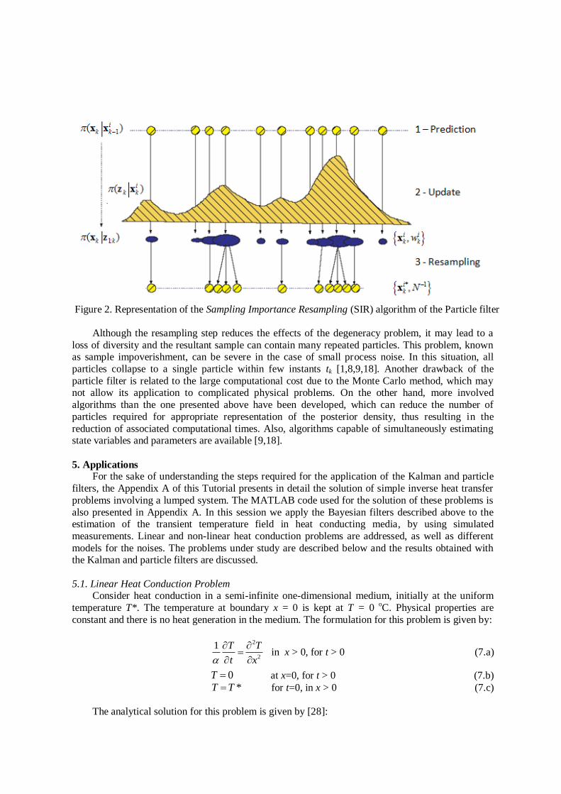
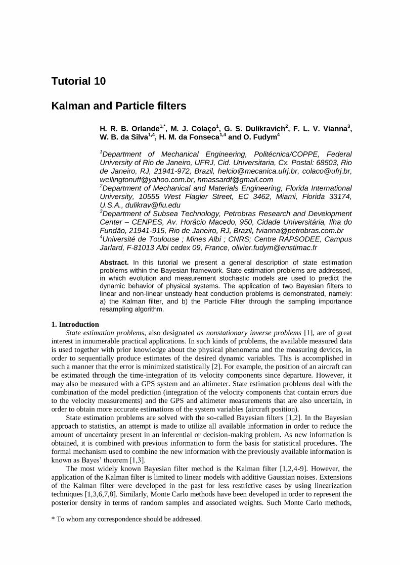
Figure 2. Representation of the Sampling Importance Resampling (SIR) algorithm of the Particle filter

Although the resampling step reduces the effects of the degeneracy problem, it may lead to a

loss of diversity and the resultant sample can contain many repeated particles. This problem, known as sample impoverishment, can be severe in the case of small process noise. In this situation, all

particles collapse to a single particle within few instants tk [1,8,9,18]. Another drawback of the

particle filter is related to the large computational cost due to the Monte Carlo method, which may not allow its application to complicated physical problems. On the other hand, more involved

algorithms than the one presented above have been developed, which can reduce the number of

particles required for appropriate representation of the posterior density, thus resulting in the

reduction of associated computational times. Also, algorithms capable of simultaneously estimating state variables and parameters are available [9,18].

5. Applications For the sake of understanding the steps required for the application of the Kalman and particle

filters, the Appendix A of this Tutorial presents in detail the solution of simple inverse heat transfer

problems involving a lumped system. The MATLAB code used for the solution of these problems is

also presented in Appendix A. In this session we apply the Bayesian filters described above to the estimation of the transient temperature field in heat conducting media, by using simulated

measurements. Linear and non-linear heat conduction problems are addressed, as well as different

models for the noises. The problems under study are described below and the results obtained with the Kalman and particle filters are discussed.

5.1. Linear Heat Conduction Problem Consider heat conduction in a semi-infinite one-dimensional medium, initially at the uniform

temperature T*. The temperature at boundary x = 0 is kept at T = 0 oC. Physical properties are

constant and there is no heat generation in the medium. The formulation for this problem is given by:

2

2

1 T T

t x

in x > 0, for t > 0 (7.a)

0T at x=0, for t > 0 (7.b)

*T T for t=0, in x > 0 (7.c)

The analytical solution for this problem is given by [28]:

( , ) *4

xT x t T erf

t

(8)

The discretization of equation (7.a) by using explicit finite-differences results in:

1

1 1(1 2 )k k k k

i i i iT rT r T rT

(9)

where the superscript k denotes the time step, the subscript i denotes the finite-difference node and

2( )

tr

x

(10)

For the solution of problem (7.a-c) with finite-differences we have to impose a boundary

condition at some fictitious surface at x=L. We assume L sufficiently large for the time range of interest, so that the finite domain behaves as a semi-infinite medium. Temperature at the surface x=L

was assumed to be T*.

The finite-difference solution for problem (7.a-c) can be written as:

1k k T FT S (11)

where

1

NT

T

T

Τ

(1 2 )

(1 2 )

(1 2 )

(1 2 )

r r

r r r

r r r

r r

F

0

0

*rT

S

(12.a-c)

In the equations above NT is the number of internal nodes in the finite-difference discretization. Matrix F is NTxNT and vectors T and S are NTx1.

Equation (11) is in appropriate form for the application of the Kalman filter (see equation 3.a).

In the present example it is assumed that state and measured variables are the transient temperatures

inside the medium at the equidistant finite difference nodes. Therefore, matrix H for the observation model (see equation 3.b) is the identity matrix.

The medium is considered to be concrete, with thermal diffusivity a = 4.9x10-7

m2/s. The

standard deviation for the measurement errors is considered constant and equal to 2 oC. The effects

of the standard deviation of the errors in the state model are examined below. Figures 3.a and 3.b

present the exact temperatures and the measured temperatures in the region, respectively. The final

time is taken as 250 seconds and measurements are supposed available in the region every 1 second.

The thickness of the medium is considered to be L = 0.1 m and the region is discretized with NT = 50 internal nodes.

Figure 3.a – Exact temperatures

Figure 3.b – Measured temperatures containing Gaussian errors with standard deviation of 2

oC

Figures 4.a,b present a comparison of exact, measured and predicted temperatures at positions

x = 0.002 m and x = 0.01 m, respectively. The predicted temperatures were obtained with the Kalman filter. The 99% confidence intervals for the predicted temperatures are also presented in these

figures. The results presented in figures 4.a,b were obtained with a standard deviation for the

evolution model errors of 1 oC. These figures clearly show a great improvement in the predicted

temperatures as compared to the measured temperatures at different positions inside the medium.

Note that predicted temperatures are much closer to the exact ones than the measurements. In fact, if

the model errors are reduced, the predicted temperatures tend to follow the model more closely. This

is exemplified in figures 5.a,b, where the standard deviation of the evolution model errors was reduced to 0.5

oC. On the other hand, if such errors are large, the predictions of the Kalman filter tend

to follow the measurements instead of the model. Such a fact is clear from the analysis of figures

6.a,b, which present the results for a standard deviation for the evolution model errors of 2 oC.

050

100150

200250

0

0.05

0.1-20

0

20

40

60

80

Time, s

Exact Temperature

x, m

T,

C

050

100150

200250

0

0.05

0.1-20

0

20

40

60

80

Time, s

Measured Temperature

x, m

T,

C

(a)

(b)

Figure 4 – Temperature at (a) x = 0.002 m and (b) x = 0.01 m – standard deviation for the evolution

model errors of 1 oC – Kalman filter

0 50 100 150 200 250-10

0

10

20

30

40

50

Time, s

T(x

=0.0

02 m

), C

Exact

Measured

Predicted

99% Confidence Interval

0 50 100 150 200 25015

20

25

30

35

40

45

50

55

60

Time, s

T(x

=0.0

1 m

), C

Exact

Measured

Predicted


(a)

(b)

Figure 5 – Temperature at (a) x = 0.002 m and (b) x = 0.01 m – standard deviation for the evolution

model errors of 0.5 oC – Kalman filter

0 50 100 150 200 250-10

0

10

20

30

40

50

60

Time, s

T(x

=0.0

02 m

), C

Exact

Measured

Predicted


0 50 100 150 200 25015

20

25

30

35

40

45

50

55

60

Time, s

T(x

=0.0

1 m

), C

Exact

Measured

Predicted


(a)

(b)

Figure 6 – Temperature at (a) x = 0.002 m and (b) x = 0.01 m – standard deviation for the evolution model errors of 5

oC – Kalman filter

The application of the particle filter with the sampling importance resampling algorithm

described above is presented in figures 7.a,b. These figures present the exact, measured and predicted temperatures at positions x = 0.002 m and x = 0.01 m, respectively. Fifty particles were used in this

0 50 100 150 200 250-10

0

10

20

30

40

50

60

Time, s

T(x

=0.0

02 m

), C

Exact

Measured

Predicted


0 50 100 150 200 25010

20

30

40

50

60

70

Time, s

T(x

=0.0

1 m

), C

Exact

Measured

Predicted


case. A comparison of figures 4.a,b and 7.a,b show that the particle filter, similarly to the Kalman

filter, provided accurate predictions for the temperature in the region. However, as expected, the computational cost of the particle filter was substantially larger than that of the Kalman filter. For

this example, the predictions obtained with the Kalman filter took 0.5 seconds and those obtained

with the particle filter took 6.9 seconds on a 1.8 GHz Centrino Duo computer with 1 Mbyte of RAM

memory.

(a)

(b)

Figure 7 – Temperature at (a) x = 0.002 m and (b) x = 0.01 m – standard deviation for the evolution model errors of 1

oC – Particle filter (SIR)

0 50 100 150 200 250-10

0

10

20

30

40

50

Time, s

T(x

=0.0

02 m

), C

Particle Filter with Re-sampling - Number of Particles = 50

Exact

Measured

Predicted


0 50 100 150 200 25015

20

25

30

35

40

45

50

55

60

Time, s

T(x

=0.0

1 m

), C


Exact

Measured

Predicted


We now examine a case involving uniformly distributed errors in the evolution model, instead

of Gaussian errors. For such case, the application of the Kalman filter does not result in optimal solutions. Consequently, only the particle filter was considered for the prediction of the temperatures

in the region. The results obtained with errors in the evolution model uniformly distributed in the

interval [-1,1] oC are presented in figures 8.a,b for x = 0.002 m and x = 0.01 m, respectively. These

figures show that the particle filter was not affected by the distribution of the errors and results similar to those obtained for the Gaussian distribution (see figures 7.a,b) were obtained.

(a)

(b)

Figure 8 – Temperature at (a) x = 0.002 m and (b) x = 0.01 m – evolution model errors having

uniform distribution in [-1,1] oC – Particle filter (SIR)

0 50 100 150 200 250-10

0

10

20

30

40

50

Time, s

T(x

=0.0

02 m

), C


Exact

Measured

Predicted


0 50 100 150 200 25015

20

25

30

35

40

45

50

55

60

Time, s

T(x

=0.0

1 m

), C


Exact

Measured

Predicted


5.2. Non-linear Heat Conduction Problem

Consider heat conduction in a one-dimensional medium with thickness L, initially at the uniform temperature T*. The boundary at x = 0 is kept insulated and a constant heat flux q* is

imposed at x = L. Thermophysical properties are temperature dependent and there is no heat

generation in the medium. The formulation for this problem is given by:

( ) ( )T T

C T k Tt x x

in 0 < x < L, for t > 0 (13.a)

0T

x

at x=0, for t > 0 (13.b)

( ) *T

k T qx

at x=L, for t > 0 (13.c)

*T T for t=0, in x > 0 (13.d)

We examine here a physical problem involving the heating of a graphite sample with an oxy-

acetylene torch [19]. The temperature dependence of the thermal conductivity, k(T), and volumetric heat capacity, C(T), of the graphite, measured for different temperatures, were curve-fitted (see

figure 9) with exponentials of the form:

3

1 2

T AC T A A e

(14.a)

3

1 2

T Bk T B B e

(14.b)

with the adjusted parameters A1, A2, A3, B1, B2 and B3 given in table 1.

Table 1. Parameters of the curve-fitted thermophysical properties

Parameter Mean

A1 (Jm-3

ºC-1

) 5,681,006

A2 (Jm-3

ºC-1

) 4,813,057

A3 (ºC) 547.00

B1 (Wm-1

ºC-1

) 24.52

B2 (Wm-1

ºC-1

) 183.05

B3 (ºC) 277.00

Figure 9. Temperature-dependent thermophysical properties

The sample was supposed to be initially at the room temperature of T* = 20 oC and the imposed

heat flux was q* = 105 W/m

2. The thickness of the slab was taken as L = 0.01 m. Finite volumes were

used for the solution of this nonlinear heat conduction problem, with the region discretized with 50

equal volumes. The final time was supposed to be 90 seconds and the time step was taken as 1 second. The errors in the state evolution and observation models were supposed to be additive,

Gaussian, uncorrelated, with zero mean and constant standard deviations.

In order to examine a very strict case, the standard deviation for the state evolution model was set to 5

oC and for the observation model as 10

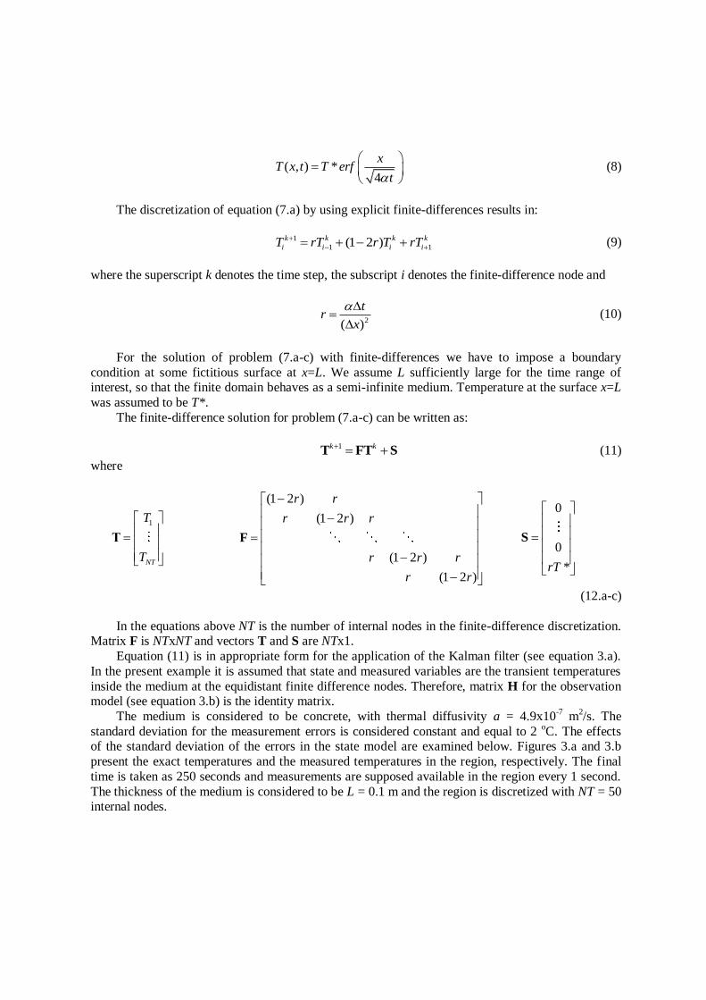
oC. Figures 10.a and 10.b present the exact and

measured temperatures, respectively, for such non linear heat conduction problem. It is apparent

from the analysis of these figures that extremely large measurement errors were considered for this

case. State evolution and measurement models were used for the prediction of the temperature

variation in the region. Due to the nonlinear character of the problem under consideration, only the

particle filter, in the form of the SIR algorithm described above, was used for the predictions. Fifty particles were used in such filtering algorithm.

Figures 11.a-d present a comparison of exact, measured and predicted temperatures at the

positions x = 0.0002 m, 0.001 m, 0.002 m and 0.004 m, respectively. An analysis of these figures reveals the robustness of the particle filter. Despite the very large errors in the evolution and

observation models, the predicted average temperatures are in excellent agreement with the exact

values. Furthermore, the 99% confidence intervals for the predicted temperatures are significantly

smaller than the dispersion of the measurements. Differently from the case analyzed above involving linear heat conduction, sample impoverishment is not observed in figures 11.a-d. This is probably

due to the large noise in the state model used for the nonlinear case. The computational time for this

case was 61.3 seconds.

0

20

40

60

80

100

120

140

160

180

200

0 500 1000 1500 2000 2500

1x106

2x106

3x106

4x106

5x106

6x106

Capacidade térm ica

Ca

pa

cid

ad

e T

érm

ica

Vo

lum

etr

ica

(J

/m3.°

C)

Tem peratura (°C)

Condutividade térm ica

Co

nd

uti

vid

ad

e t

érm

ica

(W

/m.°

C)

Thermal conductivity

Heat capacity

Temperature (oC)

Th

erm

al C

ond

uctivity (

Wm

-1oC

-1)

Volu

me

tric

Hea

t C

ap

acity (

Jm

-3oC

-1)

0

20

40

60

80

100

120

140

160

180

200

0 500 1000 1500 2000 2500

1x106

2x106

3x106

4x106

5x106

6x106

Capacidade térm ica

Ca

pa

cid

ad

e T

érm

ica

Vo

lum

etr

ica

(J

/m3.°

C)

Tem peratura (°C)

Condutividade térm ica

Co

nd

uti

vid

ad

e t

érm

ica

(W

/m.°

C)

Thermal conductivity

Heat capacity

Temperature (oC)

Th

erm

al C

ond

uctivity (

Wm

-1oC

-1)

Volu

me

tric

Hea

t C

ap

acity (

Jm

-3oC

-1)

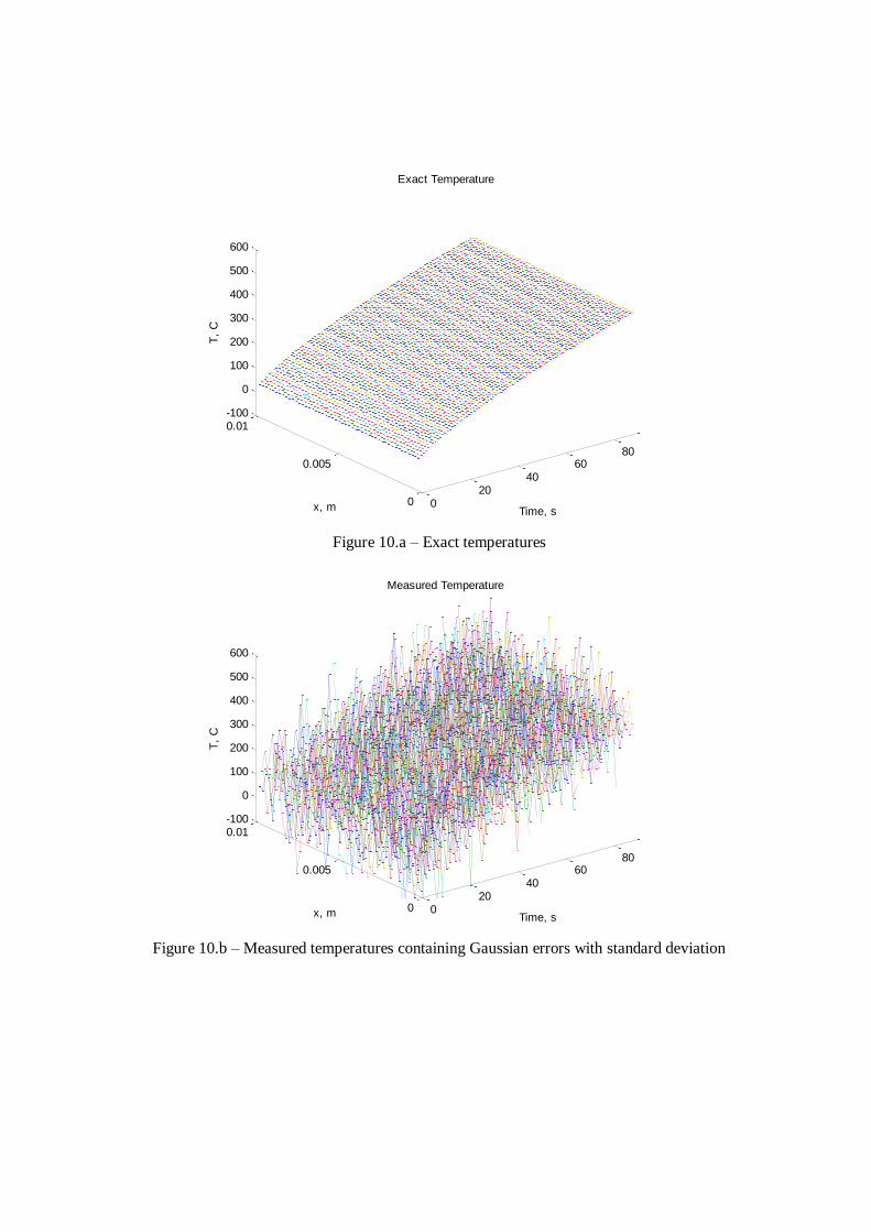
Figure 10.a – Exact temperatures

Figure 10.b – Measured temperatures containing Gaussian errors with standard deviation

020

4060

80

0

0.005

0.01-100

0

100

200

300

400

500

600

Time, s

Exact Temperature

x, m

T,

C

020

4060

80

0

0.005

0.01-100

0

100

200

300

400

500

600

Time, s

Measured Temperature

x, m

T,

C

Figure 11.a – Temperature at x = 0.0002 m for the nonlinear heat conduction problem – Particle filter

Figure 11.b – Temperature at x = 0.001 m for the nonlinear heat conduction problem – Particle filter

0 10 20 30 40 50 60 70 80 90-100

0

100

200

300

400

500

600

Time, s

T(x

=0.0

002 m

), C


Exact

Measured

Predicted


0 10 20 30 40 50 60 70 80 90-100

0

100

200

300

400

500

600

Time, s

T(x

=0.0

01 m

), C


Exact

Measured

Predicted


Figure 11.c – Temperature at x = 0.002 m for the nonlinear heat conduction problem – Particle filter

Figure 11.d – Temperature at x = 0.004 m for the nonlinear heat conduction problem – Particle filter

0 10 20 30 40 50 60 70 80 90-300

-200

-100

0

100

200

300

400

500

600

700

Time, s

T(x

=0.0

02 m

), C


Exact

Measured

Predicted


0 10 20 30 40 50 60 70 80 90-200

-100

0

100

200

300

400

500

600

Time, s

T(x

=0.0

04 m

), C


Exact

Measured

Predicted


6. Conclusions

This tutorial dealt with the application of the Kalman filter and of the particle filter to the estimation of the transient temperature field in linear and non-linear heat conduction problems. The

particle filter was coded in the form of the sampling importance resampling (SIR) algorithm. For

linear-Gaussian models, the Kalman filter and the particle filter provided results of similar accuracy.

However, the computational cost of the particle filter was significantly larger than that of the Kalman filter. On the other hand, in non-linear and/or non-Gaussian models the basic hypotheses required for

the application of the Kalman filter are not valid. The particle filter appears in the literature as an

accurate estimation technique of general use, including for non-linear and/or non-Gaussian models. The particle filter was successfully applied above to a non-linear heat conduction problem. Such

Monte Carlo technique provided accurate estimation results, even for a strict test-case involving very

large errors in the evolution and observation models. We note that more involved algorithms than the one presented above have been developed for the

particle filter, which can reduce the number of particles required for appropriate representation of the

posterior density, thus resulting in the reduction of associated computational times. Also, algorithms

capable of simultaneously estimating state variables and parameters are available (see [9,18]).

7. Acknowledgements

The financial support provided by FAPERJ, CAPES and CNPq, Brazilian agencies for the fostering of science, is greatly appreciated

8. References

1. Kaipio, J. and Somersalo, E., 2004, Statistical and Computational Inverse Problems, Applied Mathematical Sciences 160, Springer-Verlag.

2. Maybeck, P., 1979, Stochastic models, estimation and control, Academic Press, New York.

3. Winkler, R., 2003, An Introduction to Bayesian Inference and Decision, Probabilistic Publishing, Gainsville.

4. Kaipio, J., Duncan S., Seppanen, A., Somersalo, E., Voutilainen, A., 2005, State Estimation

for Process Imaging, Chapter in Handbook of Process Imaging for Automatic Control, editors: David Scott and Hugh McCann, CRC Press.

5. Kalman, R., 1960, A New Approach to Linear Filtering and Prediction Problems, ASME J.

Basic Engineering, vol. 82, pp. 35-45.

6. Sorenson, H., 1970, Least-squares estimation: from Gauss to Kalman, IEEE Spectrum, vol. 7, pp. 63-68.

7. Welch, G. and Bishop, G., 2006, An Introduction to the Kalman Filter, UNC-Chapel Hill,

TR 95-041. 8. Arulampalam, S., Maskell, S., Gordon, N., Clapp, T., 2001, A Tutorial on Particle Filters for

on-line Non-linear/Non-Gaussian Bayesian Tracking, IEEE Trans. Signal Processing, vol.

50, pp. 174-188. 9. Ristic, B., Arulampalam, S., Gordon, N., 2004, Beyond the Kalman Filter, Artech House,

Boston.

10. Doucet, A., Godsill, S., Andrieu, C., 2000, On sequential Monte Carlo sampling methods for

Bayesian filtering, Statistics and Computing, vol. 10, pp. 197-208. 11. Liu, J and Chen, R., 1998, Sequential Monte Carlo methods for dynamical systems, J.

American Statistical Association, vol. 93, pp. 1032-1044.

12. Andrieu, C., Doucet, A., Robert, C., 2004, Computational advances for and from Bayesian analysis, Statistical Science, vol. 19, pp. 118-127.

13. Johansen, A. Doucet, A., 2008, A note on auxiliary particle filters, Statistics and Probability

Letters, to appear.

14. Carpenter, J., Clifford, P., Fearnhead, P, 1999, An improved particle filter for non-linear problems, IEEE Proc. Part F: Radar and Sonar Navigation, vol. 146, pp. 2-7.

15. Del Moral, P., Doucet, A., Jasra, A., 2007, Sequential Monte Carlo for Bayesian

Computation, Bayesian Statistics, vol. 8, pp. 1-34. 16. Del Moral, P., Doucet, A., Jasra, A., 2006, Sequential Monte Carlo samplers, J. R. Statistical

Society, vol. 68, pp. 411-436.

17. Andrieu, C., Doucet, Sumeetpal, S., Tadic, V., 2004, Particle methods for charge detection,

system identification and control, Proceedings of IEEE, vol. 92, pp. 423-438. 18. Doucet, A., Freitas, N and Gordon, N., 2001, Sequential Monte Carlo Methods in Practice,

Springer, New York.

19. Orlande, H., Dulikravich, G. and Colaço, M., 2008, Application of Bayesian Filters to Heat Conduction Problem, EngOpt 2008 – International Conference on Eng. Optimization, (ed:

Herskovitz), June 1-5, Rio de Janeiro, Brazil.

20. Silva, W. B. Orlande, H. R. B.; Colaço, M. J., 2010, .Evaluation of Bayesian Filters Applied to Heat Conduction Problems, 2nd International Conference on Engineering Optimization,

Lisboa.

21. Silva, W. B. Orlande, H. R. B.; Colaço, M. J., Fudym, O., 2011, Application Of Bayesian

Filters To A One-Dimensional Solidification Problem, 21st Brazilian Congress of Mechanical Engineering, Natal, RN, Brazil.

22. Colaço, M. J., Orlande, H. R. B.; Silva, W. B., Dulikravich, G., 2011, Application Of A

Bayesian Filter To Estimate Unknown Heat Fluxes In A Natural Convection Problem, ASME 2011 International Design Engineering Technical Conferences & Computers and

Information in Engineering Conference, IDETC/CIE 2011, August 29-31, Washington, DC.

23. Fonseca, H., Orlande, H. R. B., Fudym, O., Sepulveda, F., 2010, Kalman Filtering For

Transient Source Term Mapping From Infrared Images, Inverse Problems, Design And Optimization Symposium, João Pessoa.

24. Vianna, F., Orlande, H. R. B., Dulikravich, G., 2010, Optimal Heating Control To Prevent

Solid Deposits In Pipelines, V European Conference On Computational Fluid Dynamics - ECCOMAS CFD 2010

25. Vianna, F., Orlande, H. R. B., Dulikravich, G., 2010, Pipeline Heating Method Based On

Optimal Control And State Estimation, Brazilian Congress Of Thermal Sciences And Engineering, Uberlândia.

26. Vianna, F., Orlande, H. R. B., Dulikravich, G, 2010, Temperature Field Prediction Of A

Multilayered Composite Pipeline Based On The Particle Filter Method, 14th International

Heat Transfer Conference, Washington. 27. Vianna, F., Orlande, H. R. B., Dulikravich, G, 2009, Estimation Of The Temperature Field

In Pipelines By Using The Kalman Filter, 2nd International Congress of Serbian Society of

Mechanics (IConSSM 2009) 28. Ozisik, M., 1993, Heat Conduction, Wiley, New York.

Appendix A In this appendix, for didactical purposes, we present the solution of a simple state estimation

problem in heat transfer, involving a lumped system. The problem is formulated and solved below,

by using the Kalman filter and the Particle filter, coded with the SIR algorithm. Two different cases are examined and a MATLAB code is included.

Physical Problem and Mathematical Formulation

We consider a slab of thickness L, initially at the uniform temperature T0, which is subjected to a uniform heat flux q(t) over one of its surfaces, while the other exchanges heat by convection and

linearized radiation with a medium at a temperature T with a heat transfer coefficient h (see figure

A.1). Temperature gradients are neglected inside the slab and a lumped formulation is used. The

formulation for this problem is given by [1]:

( ) ( )( )

d t mq tm t

dt h

for t > 0 (A.1.a)

0 for t = 0 (A.1.b)

where

( ) ( )t T t T (A.2.a)

0 0T T (A.2.b)

hm

c L (A.2.c)

and is the density and c is the specific heat of the homogeneous material of the slab.

Figure A.1. Physical problem [1]

Two illustrative cases are now examined, namely: (i) Heat Flux q(t) = q0 constant and deterministically known; and (ii) Heat Flux q(t) = q0 f(t) with unknown time variation. Results are

obtained for these two cases, by assuming that the plate is made of aluminum (kgm-3

, c =

896 Jkg-1

K-1

), with thickness L = 0.03 m, q0 = 8000 Wm-2

, T =20 oC, h = 50 Wm

-2K

-1 and T0 = 50

oC

[1]. Measurements of the transient temperature of the slab are assumed available. These

measurements contain additive, uncorrelated, Gaussian errors, with zero mean and a constant

standard deviation z. The errors in the state evolution model are also supposed to be additive,

uncorrelated, Gaussian, with zero mean and a constant standard deviation .

(i) Heat Flux q(t) = q0 constant and deterministically known

The analytical solution for this problem is given by:

00( ) (1 )mt mtq

t e eh

(A.3)

The only state variable in this case is the temperature ( )k kt since the applied heat flux q0 is

constant and deterministically known, as the other parameters appearing in the formulation. By using

a forward finite-differences approximation for the time derivative in equation (A.1.a), we obtain:

01(1 )k k

mqm t t

h (A.4)

Therefore, the state and observation models given by equations (3.a,b) are obtained with:

[ ]k kx

[(1 )]k m t F

0k

qm t

h

s

[1]k H

2[ ]k Q

2[ ]k zR (A5.a-f)

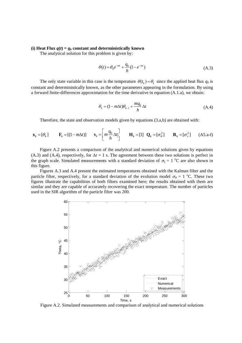
Figure A.2 presents a comparison of the analytical and numerical solutions given by equations

(A.3) and (A.4), respectively, for t = 1 s. The agreement between these two solutions is perfect in

the graph scale. Simulated measurements with a standard deviation of z = 1 oC are also shown in

this figure.

Figures A.3 and A.4 present the estimated temperatures obtained with the Kalman filter and the

particle filter, respectively, for a standard deviation of the evolution model = 1 oC. These two

figures illustrate the capabilities of both filters examined here; the results obtained with them are similar and they are capable of accurately recovering the exact temperature. The number of particles

used in the SIR algorithm of the particle filter was 200.

Figure A.2. Simulated measurements and comparison of analytical and numerical solutions

0 50 100 150 200 250 30025

30

35

40

45

50

55

60

Time, s

Theta

, °C

Exact

Numerical

Measurements

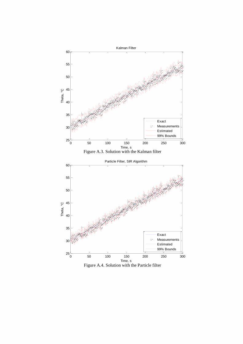
Figure A.3. Solution with the Kalman filter

Figure A.4. Solution with the Particle filter

0 50 100 150 200 250 30025

30

35

40

45

50

55

60

Time, s

Theta

, °C

Kalman Filter

Exact

Measurements

Estimated

99% Bounds

0 50 100 150 200 250 30025

30

35

40

45

50

55

60

Time, s

Theta

, °C

Particle Filter, SIR Algorithm

Exact

Measurements

Estimated

99% Bounds

(ii) Heat Flux q(t) = q0 f(t) with unknown time variation

The analytical solution for this problem is given by:

00

0

( ) ( )

t

mt mt

t

mqt e e f t dt

h

(A.6)

In this case, the state variables are given by the temperature ( )k kt and the function that

gives the time variation of the applied heat flux, that is, ( )k kf t f .As in the case examined above,

the applied heat flux q0 is constant and deterministically known, as the other parameters appearing in the formulation. By using a forward finite-differences approximation for the time derivative in

equation (A.1.a), we obtain the equation for the evolution of the state variable ( )k kt :

01 1(1 )k k k

mqm t t f

h

(A.7)

A random walk model is used for the state variable ( )k kf t f , which is given in the form:

1 1k k kf f (A.8)

where k-1 is Gaussian with zero mean and constant standard deviation rw. Therefore, the state and observation models given by equations (3.a,b) are obtained with:

k

k

kf

x

0(1 )

0 1k

mqm t t

h

F

0

0k

s

(A.9.a-c)

[1 0]k H

2

2

0

0k

rw

Q

2[ ]k zR

(A.9.d-f)

For the cases studied here, two different functions were examined for the time variation of the applied heat flux, specifically, a step function in the form:

1, 02

( )

0,2

final

final

final

tt

f tt

t t

(A.10)

and a ramp function in the form

( )final

tf tt

(A.11)

Figure A.5 presents a comparison of the analytical and numerical solutions given by equations (A.6) and (A.7), respectively, for the step variation of the heat flux. Figure A.6 presents a similar

comparison for the ramp variation of the heat flux. For both cases, we took t = 1 s. The agreement between these two solutions for both cases is perfect in the graph scale. Simulated measurements

with a standard deviation of z = 1 oC are also shown in these figures.

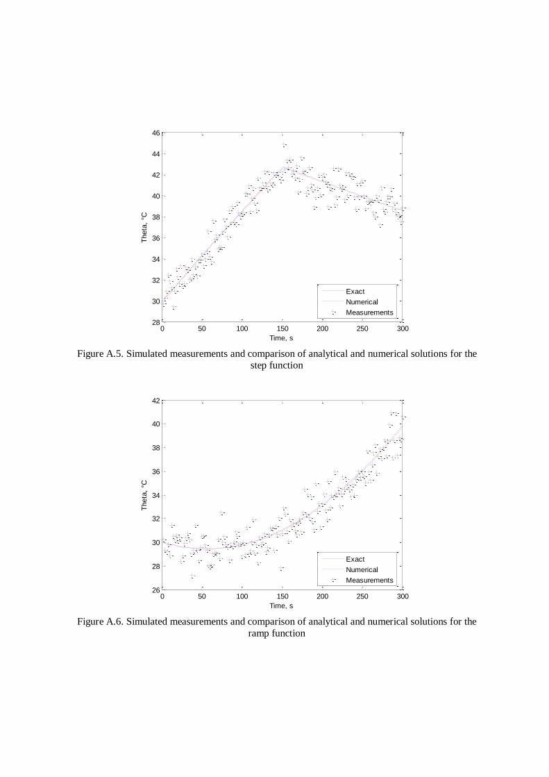
Figure A.5. Simulated measurements and comparison of analytical and numerical solutions for the

step function

Figure A.6. Simulated measurements and comparison of analytical and numerical solutions for the

ramp function

0 50 100 150 200 250 30028

30

32

34

36

38

40

42

44

46

Time, s

Theta

, °C

Exact

Numerical

Measurements

0 50 100 150 200 250 30026

28

30

32

34

36

38

40

42

Time, s

Theta

, °C

Exact

Numerical

Measurements

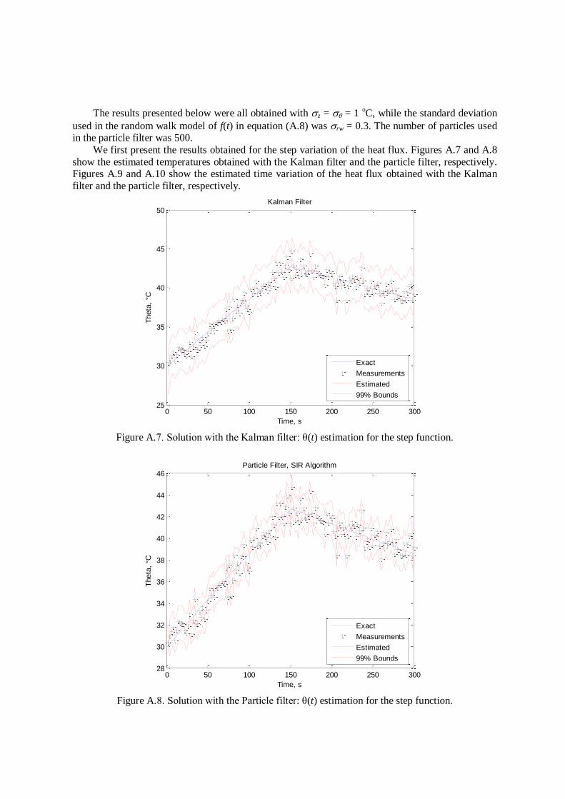
The results presented below were all obtained with z = = 1 oC, while the standard deviation

used in the random walk model of f(t) in equation (A.8) was rw = 0.3. The number of particles used in the particle filter was 500.

We first present the results obtained for the step variation of the heat flux. Figures A.7 and A.8

show the estimated temperatures obtained with the Kalman filter and the particle filter, respectively. Figures A.9 and A.10 show the estimated time variation of the heat flux obtained with the Kalman

filter and the particle filter, respectively.

Figure A.7. Solution with the Kalman filter: θ(t) estimation for the step function.

Figure A.8. Solution with the Particle filter: θ(t) estimation for the step function.

0 50 100 150 200 250 30025

30

35

40

45

50

Time, s

Theta

, °C

Kalman Filter

Exact

Measurements

Estimated

99% Bounds

0 50 100 150 200 250 30028

30

32

34

36

38

40

42

44

46

Time, s

Theta

, °C


Exact

Measurements

Estimated

99% Bounds

Figure A.9. Solution with the Kalman filter: f(t) estimation for the step function.

Figure A.10. Solution with the Particle filter: f(t) estimation for the step function.

The results obtained for the ramp variation of the heat flux are presented in figures A.11-A.14.

Figures A.11 and A.12 show the estimated temperatures obtained with the Kalman filter and the particle filter, respectively. Figures A.13 and A.14 show the estimated time variation of the heat flux

obtained with the Kalman filter and the particle filter, respectively

0 50 100 150 200 250 300-1.5

-1

-0.5

0

0.5

1

1.5

2

2.5

Time, s

f ,

no u

nits

Kalman Filter - f estimation

Exact

Estimated

99% Bounds

0 50 100 150 200 250 300-1

-0.5

0

0.5

1

1.5

2

2.5

Time, s

f ,

no u

nits

Particle Filter, SIR Algorithm - f estimation

Exact

Estimated

99% Bounds

Figure A.11. Solution with the Kalman filter: θ(t) estimation for the ramp function.

Figure A.12. Solution with the Particle filter: θ(t) estimation for the ramp function.

0 50 100 150 200 250 30024

26

28

30

32

34

36

38

40

42

44

Time, s

Theta

, °C

Kalman Filter

Exact

Measurements

Estimated

99% Bounds

0 50 100 150 200 250 30026

28

30

32

34

36

38

40

42

Time, s

Theta

, °C


Exact

Measurements

Estimated

99% Bounds

Figure A.13. Solution with the Kalman filter: f(t) estimation for the ramp function.

Figure A.14. Solution with the Particle filter: f(t) estimation for the ramp function.

Figures A.7-A.14 illustrate the capabilities of both filters examined here, for the simultaneous

estimation of the transient temperature and of the time variation of the applied heat flux. Note that measurements are available only for the temperature, and that a non-informative random walk model

was used for the variation of the heat flux. For both variations of the heat flux, and with both filters,

the recovered heat fluxes show oscillations due to the ill-posed character of the inverse problem (see figures A.9 and A.10 for the step function and A.13 and A.14 for the ramp function). Such

oscillations can be reduced by decreasing the standard deviation used for the random walk model for

f(t) (see equation A.8), resulting in smoother recovered functions. On the other hand, fast variations

0 50 100 150 200 250 300-1.5

-1

-0.5

0

0.5

1

1.5

2

Time, s

f ,

no u

nits


Exact

Estimated

99% Bounds

0 50 100 150 200 250 300-1.5

-1

-0.5

0

0.5

1

1.5

2

Time, s

f ,

no u

nits


Exact

Estimated

99% Bounds

cannot be resolved. This fact is illustrated in figures A.15-A.18 for the step variation of the heat flux,

where rw was taken as 0.1, instead of 0.3 as above (see also figures A.7-A.10).

Figure A.15. Solution with the Kalman filter: θ(t) estimation for the step function.

Figure A.16. Solution with the Particle filter: θ(t) estimation for the step function.

0 50 100 150 200 250 30025

30

35

40

45

50

Time, s

Theta

, °C

Kalman Filter

Exact

Measurements

Estimated

99% Bounds

0 50 100 150 200 250 30028

30

32

34

36

38

40

42

44

46

Time, s

Theta

, °C


Exact

Measurements

Estimated

99% Bounds

Figure A.17. Solution with the Kalman filter: f(t) estimation for the step function.

Figure A.18. Solution with the Particle filter: f(t) estimation for the step function.

The MATLAB code used for the cases presented above can be found at the end of this

Appendix.

References 1. Bayazitoglu, Y., Ozisik, M., 1988, Elements of Heat Transfer, McGraw Hill, New York.

0 50 100 150 200 250 300-0.2

0

0.2

0.4

0.6

0.8

1

1.2

1.4

Time, s

f ,

no u

nits


Exact

Estimated

99% Bounds

0 50 100 150 200 250 300-0.2

0

0.2

0.4

0.6

0.8

1

1.2

1.4

1.6

Time, s

f ,

no u

nits


Exact

Estimated

99% Bounds

MATLAB code for Case (i): Heat Flux q(t) = q0 is constant and deterministically known, and

(ii): Heat Flux q(t) = q0 f(t) is a state variable %%%%%%%%%%%%%%%%%%%%%%%%%%%%%%%%%%%%%%%%%%%%%%%%%%%%%%%%%%%%%%%%%%%%%%%%%%%

% Example for the Kalman Filter and the Particle Filter (SIR Algorithm) %

% %

% Slab of thickness L with lumped formulation - Example 2-4, Bayazitoglu%

% and Ozisik's book - page 26 %

% %

% Helcio R. B. Orlande, Henrique M. da Fonseca and Wellington B. da Silva% % June 01, 2011 %

% %

%%%%%%%%%%%%%%%%%%%%%%%%%%%%%%%%%%%%%%%%%%%%%%%%%%%%%%%%%%%%%%%%%%%%%%%%%%%

clc

clear all;

close all;

%%%%%%%%%%%%%%%%%%%%%%%%%%%%%%%%%%%%%%%%%%%%%%%%%%%%%%%%%%%%%%%%%%%%%%%%%%%

% physical parameters of the medium %

%%%%%%%%%%%%%%%%%%%%%%%%%%%%%%%%%%%%%%%%%%%%%%%%%%%%%%%%%%%%%%%%%%%%%%%%%%%

k = 204; % thermal conductivity, W/mK

ro = 2707; % density, kg/m^3

cp = 896; % spcific heat, J/kgK

lthick = 0.03; % thickness of the plate, m

%%%%%%%%%%%%%%%%%%%%%%%%%%%%%%%%%%%%%%%%%%%%%%%%%%%%%%%%%%%%%%%%%%%%%%%%%%%

% time discretization %

%%%%%%%%%%%%%%%%%%%%%%%%%%%%%%%%%%%%%%%%%%%%%%%%%%%%%%%%%%%%%%%%%%%%%%%%%%%

timefinal=300; % final time, s

deltatime=1; % time step, s

time=deltatime:deltatime:timefinal; % vector of physical time, s

%%%%%%%%%%%%%%%%%%%%%%%%%%%%%%%%%%%%%%%%%%%%%%%%%%%%%%%%%%%%%%%%%%%%%%%%%%%

% parameters for the equation %

%%%%%%%%%%%%%%%%%%%%%%%%%%%%%%%%%%%%%%%%%%%%%%%%%%%%%%%%%%%%%%%%%%%%%%%%%%%

temp0 = 50; % initial temperature, oC

q0 = 8000; % applied heat flux, W/m^2

tempinf=20; % external temperature, oC

htcoef=50; % heat transfer coefficient, W/m^2K

mcoef=htcoef/(ro*cp*lthick);

q0h=q0/htcoef;

theta0=temp0-tempinf;

%%%%%%%%%%%%%%%%%%%%%%%%%%%%%%%%%%%%%%%%%%%%%%%%%%%%%%%%%%%%%%%%%%%%%%%%%%%

% number of particles for the Particle Filter %

%%%%%%%%%%%%%%%%%%%%%%%%%%%%%%%%%%%%%%%%%%%%%%%%%%%%%%%%%%%%%%%%%%%%%%%%%%%

Nparti=200;

Nparti1=1/Nparti;

%%%%%%%%%%%%%%%%%%%%%%%%%%%%%%%%%%%%%%%%%%%%%%%%%%%%%%%%%%%%%%%%%%%%%%

% std for the measurement error, evolution model and random walk %

%%%%%%%%%%%%%%%%%%%%%%%%%%%%%%%%%%%%%%%%%%%%%%%%%%%%%%%%%%%%%%%%%%%%%%

stdmeas=0.3; % standard deviation of the measurement errors

stdmodel=0.03; % standard deviation of the evolution model

stdrw=0.03; % random walk of the estimated parameter

%%%%%%%%%%%%%%%%%%%%%%%%%%%%%%%%%%%%%%%%%%%%%%%%%%%%%%%%%%%%%%%%%%%%%%%%%%%

% Choose of the structure of the function f %

% %

% 1 = Constant function over all the experiment %

% 2 = Square time varying function %

% 3 = Ramp function %

% %

%%%%%%%%%%%%%%%%%%%%%%%%%%%%%%%%%%%%%%%%%%%%%%%%%%%%%%%%%%%%%%%%%%%%%%%%%%%

hf_type=3; % choose the function type

%%%%%%%%%%%%%%%%%%%%%%%%%%%%%%%%%%%%%%%%%%%%%%%%%%%%%%%%%%%%%%%%%%%%%%%%%%%

% Initializing vectors for constant heat flux %

%%%%%%%%%%%%%%%%%%%%%%%%%%%%%%%%%%%%%%%%%%%%%%%%%%%%%%%%%%%%%%%%%%%%%%%%%%%

if hf_type==1

thetanum=zeros(1,length(time));

xest=zeros(1,length(time));

P=zeros(1,length(time));

xestpf=zeros(1,length(time));

xestsir=zeros(1,length(time));

stdsir=zeros(1,length(time));

xpartiold=zeros(1,length(Nparti));

xpartinew=zeros(1,length(Nparti));

wparti=zeros(1,length(Nparti));

xpartires=zeros(1,length(Nparti));

wpartires=zeros(1,length(Nparti));

end

%%%%%%%%%%%%%%%%%%%%%%%%%%%%%%%%%%%%%%%%%%%%%%%%%%%%%%%%%%%%%%%%%%%%%%%%%%%

% Initializing vectors for time varying heat flux %

%%%%%%%%%%%%%%%%%%%%%%%%%%%%%%%%%%%%%%%%%%%%%%%%%%%%%%%%%%%%%%%%%%%%%%%%%%%

if hf_type==2||hf_type==3

thetanum=zeros(1,length(time));

xest=zeros(2,length(time));

P=zeros(2,2,length(time));

xestpf=zeros(2,length(time));

xestsir=zeros(2,length(time));

stdsir=zeros(2,length(time));

xpartiold=zeros(2,length(Nparti));

xpartinew=zeros(2,length(Nparti));

wparti=zeros(1,length(Nparti));

xpartires=zeros(2,length(Nparti));

wpartires=zeros(1,length(Nparti));

end

%%%%%%%%%%%%%%%%%%%%%%%%%%%%%%%%%%%%%%%%%%%%%%%%%%%%%%%%%%%%%%%%%%%%%%%%%%%

% form of function %

%%%%%%%%%%%%%%%%%%%%%%%%%%%%%%%%%%%%%%%%%%%%%%%%%%%%%%%%%%%%%%%%%%%%%%%%%%%

%%%%%%%%%%%%%%%%

% constant f %

%%%%%%%%%%%%%%%%

if hf_type==1

f=ones(1,(1/deltatime)*timefinal) ;

end

%%%%%%%%%%%%%%%%

% step f %

%%%%%%%%%%%%%%%%

if hf_type==2

f=[ones(1,(1/deltatime)*timefinal/2)...

zeros(1,(1/deltatime)*timefinal/2)];

end

%%%%%%%%%%%%%%%%

% ramp f %

%%%%%%%%%%%%%%%%

if hf_type==3

f=(1:deltatime:timefinal)/timefinal ; % ramp

end

%%%%%%%%%%%%%%%%%%%%%%%%%%%%%%%%%%%%%%%%%%%%%%%%%%%%%%%%%%%%%%%%%%%%%%%%%%%

% Exact Solution %

%%%%%%%%%%%%%%%%%%%%%%%%%%%%%%%%%%%%%%%%%%%%%%%%%%%%%%%%%%%%%%%%%%%%%%%%%%%

%%%%%%%%%%%%%%%%

% constant f %

%%%%%%%%%%%%%%%%

if hf_type==1

thetaexa = theta0*exp(-mcoef.*time)+q0h.*(1-exp(-mcoef.*time));

end

%%%%%%%%%%%%%%%%

% step f %

%%%%%%%%%%%%%%%%

if hf_type==2

Int=[(exp(mcoef.*(1:deltatime:(timefinal/2)))-1)...

(exp(mcoef.*timefinal/2)-1)*ones(1,(1/deltatime)*timefinal/2)] ;

thetaexa = exp(-mcoef.*time).*(theta0+q0h.*Int);

end

%%%%%%%%%%%%%%%%

% ramp f %

%%%%%%%%%%%%%%%%

if hf_type==3

thetaexa = exp(-mcoef.*time).*(theta0+q0h.*...

((1+exp(mcoef.*time).*(mcoef.*time-1))/(timefinal*mcoef)));

end

%%%%%%%%%%%%%%%%%%%%%%%%%%%%%%%%%%%%%%%%%%%%%%%%%%%%%%%%%%%%%%%%%%%%%%%%%%%

% Numerical solution (finite differece) %

%%%%%%%%%%%%%%%%%%%%%%%%%%%%%%%%%%%%%%%%%%%%%%%%%%%%%%%%%%%%%%%%%%%%%%%%%%%

bigq=mcoef*q0h*deltatime;

thetanum(1)=theta0;

for k = 1:(length(time)-1)

thetanum(k+1)=(1-mcoef*deltatime)*thetanum(k)+bigq*f(k);

end

%%%%%%%%%%%%%%%%%%%%%%%%%%%%%%%%%%%%%%%%%%%%%%%%%%%%%%%%%%%%%%%%%%%%%%%%%%%

% Simulated measurements %

%%%%%%%%%%%%%%%%%%%%%%%%%%%%%%%%%%%%%%%%%%%%%%%%%%%%%%%%%%%%%%%%%%%%%%%%%%%

unce=randn(1,length(time)); %random vector. mean=1 and std=0

thetameas=thetaexa+(stdmeas.*unce); %Tmeas=Texa+eps

%%%%%%%%%%%%%%%%%%%%%%%%%%%%%%%%%%%%%%%%%%%%%%%%%%%%%%%%%%%%%%%%%%%%%%%%%%%

% Kalman Filter %

%%%%%%%%%%%%%%%%%%%%%%%%%%%%%%%%%%%%%%%%%%%%%%%%%%%%%%%%%%%%%%%%%%%%%%%%%%%

%%%%%%%%%%%%%%%%%%%%%%%%%%%%

% constant f %

%%%%%%%%%%%%%%%%%%%%%%%%%%%%

if hf_type==1

F=(1-mcoef*deltatime);

S=bigq;

H=1;

Q=stdmodel^2;

R=stdmeas^2;

%%%%%%%%%%%%%%%%%%%%%%%%%%%%%%%%%%%%%%%%%%%%%%%%%%%%%%%%%%

%Initial State and its Covariance Matrix %

%%%%%%%%%%%%%%%%%%%%%%%%%%%%%%%%%%%%%%%%%%%%%%%%%%%%%%%%%%

xminus(1)=theta0+randn*stdmeas;

xest(1)=xminus(1);

P(1)=R;


%%%%%%%%%%%%%%%%%%%%%%%

% Prediction Kalman %

%%%%%%%%%%%%%%%%%%%%%%%

xminus=F*xest(k)+S;

Pminus=F*P(k)*F'+Q;

%%%%%%%%%%%%%%%%%%%%%%

% Update Kalman %

%%%%%%%%%%%%%%%%%%%%%%

Gainm=Pminus*H'*inv(H*Pminus*H'+R); %#ok<*MINV>

xest(k+1)=xminus+Gainm*(thetameas(k+1)-H*xminus);

P(k+1)=(eye(1)-Gainm*H)*Pminus;

end

%%%%%%%%%%%%%%%%%%%%%%%%%%%%

%Confidence interval %

%%%%%%%%%%%%%%%%%%%%%%%%%%%%

lbd=xest-2.576.*sqrt(P);

ubd=xest+2.576.*sqrt(P);

end % of the Kalman Filter estimation for a constant heat flux

%%%%%%%%%%%%%%%%%%%%%%%%%%%%

% time varying f %

%%%%%%%%%%%%%%%%%%%%%%%%%%%%

if hf_type==2 || hf_type==3

F=[(1-mcoef*deltatime) (mcoef*deltatime*q0h);0 1];

H=[1 0];

Q=[stdmodel^2 0 ;...

0 stdrw^2];

R=stdmeas^2;

%%%%%%%%%%%%%%%%%%%%%%%%%%%%%%%%%%%%%%%%%%%%%%%%%%%%%%%%%%%%%%%%%

% Initial State and its Covariance Matrix %

% %%%%%%%%%%%%%%%%%%%%%%%%%%%%%%%%%%%%%%%%%%%%%%%%%%%%%%%%%%%%%%%

xminus=[theta0+randn*stdmeas;

f(1)+randn*stdrw];

Pminus=Q;

xest(:,1)=xminus;

P(:,:,1)=Pminus;


%%%%%%%%%%%%%%%%%%%%%%%

% Prediction Kalman %

%%%%%%%%%%%%%%%%%%%%%%%

xminus=F*xminus;

Pminus=F*Pminus*F'+Q;

%%%%%%%%%%%%%%%%%%%%%%

% Update Kalman %

%%%%%%%%%%%%%%%%%%%%%%

Gainm=Pminus*H'*inv(H*Pminus*H'+R); %#ok<*MINV>

xnew=xminus+Gainm*(thetameas(k+1)-H*xminus);

Pnew=(eye(2)-Gainm*H)*Pminus;

%%%%%%%%%%%%%%%%%%%%%%%%%%%%%%%%%%%

% Storing the predicted variables %

%%%%%%%%%%%%%%%%%%%%%%%%%%%%%%%%%%%

xest(:,k+1)=xnew;

P(:,:,k+1)=Pnew;

%%%%%%%%%%%%%%%%%%%%%%%%%%%%%%%%%%

% Updating auxiliary variables %

%%%%%%%%%%%%%%%%%%%%%%%%%%%%%%%%%%

xminus=xnew;

Pminus=Pnew;

end

%%%%%%%%%%%%%%%%%%%%%%%%%%%%%

% Confidence interval %

%%%%%%%%%%%%%%%%%%%%%%%%%%%%%

lbdt=xest(1,:)-2.576.*sqrt(P(1,1));

ubdt=xest(1,:)+2.576.*sqrt(P(1,1));

lbdq=xest(2,:)-2.576.*sqrt(P(2,2));

ubdq=xest(2,:)+2.576.*sqrt(P(2,2));

end % of the Kalman Filter estimation for a time varying heat flux

%%%%%%%%%%%%%%%%%%%%%%%%%%%%%%%%%%%%%%%%%%%%%%%%%%%%%%%%%%%%%%%%%%%%%%%%%%%

% Particle Filter (SIR Algorithm) %

%%%%%%%%%%%%%%%%%%%%%%%%%%%%%%%%%%%%%%%%%%%%%%%%%%%%%%%%%%%%%%%%%%%%%%%%%%%

%%%%%%%%%%%%%%%%%%%%%%%%%%%%

% constant f %

%%%%%%%%%%%%%%%%%%%%%%%%%%%%

if hf_type==1

%%%%%%%%%%%%%%%%%%%%%%%%%%%%%

% Distribution Initial Time %

%%%%%%%%%%%%%%%%%%%%%%%%%%%%%

xestsir(1)=theta0;

for i=1:Nparti

xpartiold(i)=theta0+randn*stdmodel;

end

%%%%%%%%%%%%%%%%%%%%%%%%

% Advancing Particles %

%%%%%%%%%%%%%%%%%%%%%%%%


for i=1:Nparti

%%%%%%%%%%%%%%%%%%%%

% 1 - PREDICTION %

%%%%%%%%%%%%%%%%%%%%

xpartinew(i)=F*xpartiold(i)+S+randn*stdmodel;

%%%%%%%%%%%%%%%%%%%%

% Weights %

%%%%%%%%%%%%%%%%%%%%

wparti(i)=exp(-((xpartinew(i)-thetameas(k+1))/stdmeas)^2);

end

wtotal=sum(wparti);

wpartin=wparti./wtotal;

%%%%%%%%%%%%%%%%

% 2 - UPDATE %

%%%%%%%%%%%%%%%%

%xpartiw=xpartinew.*wparti;

%%%%%%%%%%%%%%%%%%%%%%

% Mean at time k+1 %

%%%%%%%%%%%%%%%%%%%%%%

xestpf(k+1)=xpartinew*wpartin';

%%%%%%%%%%%%%%%%%%%%%%%%%%%%%%%%%%%%

% Standard Deviation at time k+1 %

%%%%%%%%%%%%%%%%%%%%%%%%%%%%%%%%%%%%

% 3 - RESAMPLING %

%%%%%%%%%%%%%%%%%%%%%%

cresa=zeros(Nparti,1);

uresa=zeros(Nparti,1);

cresa(1)=wpartin(1);

for i=2:Nparti

cresa(i)=cresa(i-1)+wpartin(i);

end

iresa=1;

uresa(1)=rand*Nparti1;

for j=1:Nparti

uresa(j)=uresa(1)+Nparti1*(j-1);

while uresa(j) > cresa(iresa)

iresa=iresa+1;

end

xpartires(j)=xpartinew(iresa);

wpartires(j)=Nparti1;

end

%%%%%%%%%%%%%%%%%%%%%%%%%%%%%%%%%%

% Means and standard deviation %

%%%%%%%%%%%%%%%%%%%%%%%%%%%%%%%%%%

xestsir(k+1)=mean(xpartires);

stdsir(k+1)=std(xpartires);

xpartiold=xpartires;

%%%%%%%%%%%%%%%%%%%%%

% End of resampling %

%%%%%%%%%%%%%%%%%%%%%

%xpartiold=xpartinew;

end

%%%%%%%%%%%%%%%%%%%%%%%%%%%%%


%%%%%%%%%%%%%%%%%%%%%%%%%%%%%

lbdsir=xestsir-2.576.*stdsir;

ubdsir=xestsir+2.576.*stdsir;

end % of the Particle Filter estimation for a constant heat flux

%%%%%%%%%%%%%%%%%%%%%%%%%%%%%%%%

% time varying f %

%%%%%%%%%%%%%%%%%%%%%%%%%%%%%%%%

if hf_type==2 || hf_type==3

%%%%%%%%%%%%%%%%%%%%%%%%%%%%%

% Distribution Initial Time %

%%%%%%%%%%%%%%%%%%%%%%%%%%%%%

xestsir(:,1)=[theta0;f(1)];

for i=1:Nparti

xpartiold(1,i)=theta0+randn*stdmodel;

xpartiold(2,i)=f(1)+randn*stdrw;

end

%%%%%%%%%%%%%%%%%%%%%%%%

% Advancing Particles %

%%%%%%%%%%%%%%%%%%%%%%%%


for i=1:Nparti

%%%%%%%%%%%%%%%%%%%%

% 1 - PREDICTION %

%%%%%%%%%%%%%%%%%%%%

xpartinew(:,i)=F*xpartiold(:,i)+randn*[stdmodel;stdrw];

%%%%%%%%%%%%%%%%%%%%

% Weights %

%%%%%%%%%%%%%%%%%%%%

wparti(i)=exp(-((xpartinew(1,i)-thetameas(k+1))/stdmeas)^2);

end

wtotal=sum(wparti);

wpartin(1,:)=wparti./wtotal;

%%%%%%%%%%%%%%%%

% 2 - UPDATE %

%%%%%%%%%%%%%%%%

%xpartiw=xpartinew.*wparti;

%%%%%%%%%%%%%%%%%%%%%%

% Mean at time k+1 %

%%%%%%%%%%%%%%%%%%%%%%

xestpf(:,k+1)=xpartinew*wpartin';

%%%%%%%%%%%%%%%%%%%%%%%%%%%%%%%%%%%%

% Standard Deviation at time k+1 %

%%%%%%%%%%%%%%%%%%%%%%%%%%%%%%%%%%%%

% 3 - RESAMPLING %

%%%%%%%%%%%%%%%%%%%%%%

cresa=zeros(Nparti,1);

uresa=zeros(Nparti,1);

cresa(1)=wpartin(1);

for i=2:Nparti

cresa(i)=cresa(i-1)+wpartin(i);

end

iresa=1;

uresa(1)=rand*Nparti1;

for j=1:Nparti

uresa(j)=uresa(1)+Nparti1*(j-1);

while uresa(j) > cresa(iresa)

iresa=iresa+1;

end

xpartires(:,j)=xpartinew(:,iresa);

wpartires(j)=Nparti1;

end

%%%%%%%%%%%%%%%%%%%%%%%%%%%%%%%%%%

% Means and standard deviation %

%%%%%%%%%%%%%%%%%%%%%%%%%%%%%%%%%%

xestsir(1,k+1)=mean(xpartires(1,:)); % Tempearature

xestsir(2,k+1)=mean(xpartires(2,:)); % f

stdsir(1,k+1)=std(xpartires(1,:)); % Temperature

stdsir(2,k+1)=std(xpartires(2,:)); % f

xpartiold=xpartires;

%%%%%%%%%%%%%%%%%%%%%

% End of resampling %

%%%%%%%%%%%%%%%%%%%%%

%xpartiold=xpartinew;

end

%%%%%%%%%%%%%%%%%%%%%%%%%%%%%


%%%%%%%%%%%%%%%%%%%%%%%%%%%%%

lbdsirt=xestsir(1,:)-2.576.*stdsir(1,:);

ubdsirt=xestsir(1,:)+2.576.*stdsir(1,:);

lbdsirf=xestsir(2,:)-2.576.*stdsir(2,:);

ubdsirf=xestsir(2,:)+2.576.*stdsir(2,:);

end % of the Particle Filter estimation for a time varying heat flux

%%%%%%%%%%%%%%%%%%%%%%%%%%%%%%%%%%%%%%%%%%%%%%%%%%%%%%%%%%%%%%%%%%%%%%%%%%%

% plot of the results - constant f %

%%%%%%%%%%%%%%%%%%%%%%%%%%%%%%%%%%%%%%%%%%%%%%%%%%%%%%%%%%%%%%%%%%%%%%%%%%%

if hf_type==1

figure (1)

plot(time,thetaexa,'-b',time,thetanum,'--r');

xlabel('Time, s');

ylabel('Theta, °C');

legend('Exact','Numerical','Location','SouthEast');

figure (2)

plot(time,thetaexa,'-b',time,thetanum,'-r',time,thetameas,'+k');

xlabel('Time, s');


legend('Exact','Numerical','Measurements','Location','SouthEast');

figure (3)

plot(time,thetaexa,'-b',time,thetameas,'+k',time,xest,'-r',time,lbd,'--r',time,ubd,'--

r');

xlabel('Time, s');


title('Kalman Filter');

legend('Exact','Measurements','Estimated','99% Bounds','Location','SouthEast');

figure (4)

plot(time,thetaexa,'-b',time,thetameas,'+k',time,xestsir,'-r',time,lbdsir,'--

r',time,ubdsir,'--r');

xlabel('Time, s');


title('Particle Filter, SIR Algorithm');

legend('Exact','Measurements','Estimated','99% Bounds','Location','SouthEast');

end

%%%%%%%%%%%%%%%%%%%%%%%%%%%%%%%%%%%%%%%%%%%%%%%%%%%%%%%%%%%%%%%%%%%%%%%%%%%

% plot of the results - time varying f %

%%%%%%%%%%%%%%%%%%%%%%%%%%%%%%%%%%%%%%%%%%%%%%%%%%%%%%%%%%%%%%%%%%%%%%%%%%%

if hf_type==2||hf_type==3

figure (1)

plot(time,thetaexa,'-b',time,thetanum,'--r');

xlabel('Time, s');


legend('Exact','Numerical','Location','SouthEast');

figure (2)

plot(time,thetaexa,'-b',time,thetanum,'-r',time,thetameas,'+k');

xlabel('Time, s');


legend('Exact','Numerical','Measurements','Location','SouthEast');

figure (3)

plot(time,thetaexa,'-b',time,thetameas,'+k',time,xest(1,:),'-r',...

time,lbdt,'--r',time,ubdt,'--r');

xlabel('Time, s');


title('Kalman Filter');

legend('Exact','Measurements','Estimated','99% Bounds',...

'Location','SouthEast');

figure (4)

plot(time,thetaexa,'-b',time,thetameas,'+k',time,xestsir(1,:),'-r',...

time,lbdsirt,'--r',time,ubdsirt,'--r');

xlabel('Time, s');


title('Particle Filter, SIR Algorithm');

legend('Exact','Measurements','Estimated','99% Bounds',...

'Location','SouthEast');

figure (5)

plot(time,f,'-b',time,xest(2,:),'-r',time,lbdq,'--r',time,ubdq,'--r');

xlabel('Time, s');

ylabel('\itf \rm, no units');

title('Kalman Filter - \itf \rmestimation');

legend('Exact','Estimated','99% Bounds','Location','SouthEast');

figure (6)

plot(time,f,'-b',time,xestsir(2,:),'-r',time,lbdsirf,'--r',...

time,ubdsirf,'--r');

xlabel('Time, s');

ylabel('\itf \rm, no units');

title('Particle Filter, SIR Algorithm - \itf \rmestimation');

legend('Exact','Estimated','99% Bounds','Location','SouthEast');

end

Documents

Tutorial 10 Kalman and Particle filters - Semantic Scholar · Tutorial 10 Kalman and Particle filters H. 1R ... and the GPS and altimeter measurements that ... the use of the Kalman