AD-AO09 273

A REVISED COMPUTER PROGRAM FOR AXIAL COMPRESSOR DESIGN.VOLUME I. THEORY, DESCRIPTIONS, AND USER'S INSTRLUCTIONS

Richard N. Hearsey

Dayton University

Prepared for:

Aerospace Research Laboratories

January 1975

DISTRIBUTED BY:

Uh TuS. cEPiTsmT h SErICE

U. S. DEPARTMENDT OF COMMNERCE

UNCLASSIFIEDSECURITY CLASSIFICATION OF TW4IS PAGE (When DVet EntereJ)

REPORT DOUMETATIOM PAGE READ INSTRUCTIONSRT BEFORE COMPLETING FORM

I1. REPORT NUMBER 2. GOVT ACCESSION NO 3. .RECPIEINT-S CATA-.OG NUMBER

4 TITLE (and Subttle) S TYPE OF REPORT A PERIOD COVERED

A REVISED COMPUTER PROGRAM FOR Technical-FinalAXIAL COMPRESSOR DESIGN I Oct 73 -30 Nov. 1974Vol. I. Theory, Descriptions, and User's 0 PERFORMING ORO. REPORT NUMBER

Instructions UDRI-TR-74-47, Volume I7. AUTHOR(#) S. CO.oTRACT OR GRANT NUMSEW(8)

Richard M. Hearsey F33615-74-C-40309 PERFORMING ORGANIZATION NAME AND ADDRESS 10. PROGRAM ELEMENT. PROJECT. TASK

AREA & WORK UNIT NUMBERS

University of Dayton Research Institute 705027300 College Park Avenue and Project 3066Dayton. Ohio 45469

II. CONTROLLING OFFICE NAME AND ADDRESS 12. REPORT DATEAerospace Research Laboratories ARL(AFSC) January 1975Fluid Mechanics Facilities Research Lab. (LF) IS NUMBER OF PAGES121X arigh t +--P er son A FR, Oil 4543312

SMO ITORING AGENCY NAME 6 AODRESS(it diflferen hmm Conftolht Office) 1S SECURITY CLASS (oa thle report)

UnclassifiedIS. DECLASSIFICATION piOWNGRADING

SCHEDULE

IS. DISTRISUTION STATEMENT (o this RFtepor)

Approved for public release; distribution unlimited. D MIS

17 DISTRIBUTION ST ATEMENT (of the obstct entermled In Bleck 20, if dllfetent free Report)

DIS SUPPLEMENTARY NOTES

19 KEY WORDS (Conftiue an teorwoe side if necessary and id"rlfly by block number)

axial compressor ,.ordcd bytest data analysis NATIONAL TECHNICALcomputer program INFORMATION SERVICE

Us Dempo .. of C o.ejSionsoed. VA. 221S1

20 ABSTRACT (Contm*nu on reoevee•"ldt if necseesy and Identify by block number)

A revised computer program for the design of axial compressors ispresented. It comprises three principal sections, two alternative meansof determining blade geometry and an aerodynamic computation for theflow through the compressor. One method of determining blade geometryuses various analytic meanlines for the blade sections, and leads to theaerodynamic analysis of the flow through specified blading. The oth.er

DO "o* AP"73 1473 EDITION OF INOV6S IS OBSOLETE uNCLASSIFIEDSECURITY CLASSI4FICATION OF THIS PAGE fW7In Oat* Fng.cfd)

A.

UNCLASSIFIEDSECURITY CLASSIFICATION OF THIS PAGC(Wlhon Data r.nemd)

method consists of creating arbitrary blade sections to follow the flowdirections previously determined in an aerodynamic design calculation.The aerodynamic design section incorporites a loss calculation routine thatmay be used to estimate the design point performance of the compressor.One, two, or a.ll three sections may be used in any one run of the program.This first volume of two describing the program details the theory of themethod, describes the computer program, and gives all informationnecessary to use it.

A. & UNCLASSIFIEDji SECURITY CLASSIFICATION OF THIS PAG•6EW?,e Dare Ente,.Ei

PREFACE

The wo-k described in this Final Report was performed by theUniversitv •if Dayton Research Institute, 300 College Park Avenue, Dayton.Ohio 454t;9, -in-er Air Force Contract F33615-74-C-4030 during the periodOctooer 1973 to October 1974. It was a portion of Project 7065, Task 04of the Aerospace Research Laboratories, and Project 3066 of the AeroPropulsion Laboratory. Technical Monitors for the Air Force wereDr. A. J. Wennerstron,, ARL/LF, and Mr. M. A. Stibich, AFAPL/TBC,both at Wa ight-Patterson Air Force Base , Ohio 45433. This report wasinitially identified as UDRI-TR-74-47 by the University of Dayton.

iI,

TABLE OF CONTENTS

SECTION PAGE

I INTRODUCTION AND REPORT ARRANGEMENT I

11 SCOPE AND GENERAL METHOD OF PROGRAM 3

1. OVERALL PROGRAM 32. AERODYNAMIC SECTION 33. ANALYTIC MEANLINE BLADE SECTION 54. ARBITRARY MEANLINE BLADE SECTION 7

III INPUT DATA

1. DATA FORMAT 92. DATA ITEM DEFINITIONS 13

a. Initial Directives 14b. Analytic Meanline Blade Section 14c. Aerodynamic Section 22d. Arbitrary Meanline Blade Section 35

IV OUTPUT DATA 39

1. ANALYTIC MEANLINE SECTION 39Z. AERODYNAMIC SECTION 42

a. Regular Printed Output 42b. Diagnostic Printed Output 44c. Punched Card Output 50d. Precision Plot Output 51

3. ARBITRARY MEANLINE SECTION 51

V THEORY OF AERODYNAMIC ANALYSIS 54

1. MOMENTUM EQUATION 542. CONTINUITY EQUATION 613. FLUID PROPERTIES 644. RELATIVE TOTAL PRESSURE LOSS 65

COEFFICIENTS5. ENTHALPY AND ROTHALPY, AND 65

RELATED DEFINITIONS6. ANNULUS WALL BOUNDARY LAYERS 667. LOSS COEFFICIENT RE-ESTIMATION 67

iii

TABLE OF CONTENTS (Continued)

SECTION PAGE

8. OFF-DESIGN ANALYSIS SCHEME 68

(NWORK = 7)9. BLADE GEOMETRY 69

10. INTEGRATED PERFORMANCE 6911. RADIAL TRANSFER OF BLADE WAKES 7012. TURBULENT MIXING OF THE AXISYMMETRIC 73

FLOW

VI NUMERICAL PROCEDURES FOR AERODYNAMIC 77ANALYSIS

1. INTEGRATION OF DESIGN MOMENTUM 77EQUATION

2. INTEGRATION OF ANALYSIS MOMENTUM 80EQUATION

3. SATISFACTION OF CONTINUITY EQUATION 81

4. STREAMLINE RELOCATION ITERATION 82

5. CONVERGENCE CRITERIA 866. PRANDTL-MEYER FUNCTION 877. STAGNATION POINT PROVISION 88

8. INTERPOLATION 889. DEVIATION ANGLE DETERMINATION FOR 88

ANALYTIC MEANLINE BLADE SECTION10. TURBULENT MIXING CALCULATION 90

PROCEDURE

VII PROGRAM OPERATION AND STRUCTURE 96

1. IMPLEMENTATION 962. PROGRAM LOGIC 97

a. Resident 97b. Aerodynamic Section 97c. Analytic Meanline Blade Section 99d. Arbitrary Meanline Blade Section 99

3. PROGRAM AND SUBPROGRAM DESCRIPTIONS 101

a. Program UD0300 101b. Program UD03AR 101c. Program UD0301 104d. Subroutine UD0302 104

iv

TABLE OF CONTENTS (Continued)

SECTION PAGE

e. Subroutine UD0303 104f. Subroutine UD0304 104g. Subroutine UD0329 104h. Subroutine UD0305 104i. Subroutine UD0306 104j. Subroutine UD0330 104k. Subroutine UD0307 1041. Subroutine UD0309 106m. Subroutine UD0310 107n. Subroutine UD0311 107o. Subroutine UD0311 107p. Subroutine UDGI 108

q. Function UDG2 through UDG9. 108r. Subroutine UD0325 108

s. Subroutine UD0308 108t. Subroutine UD03Z6 l11u. Subroutine UD03AN 111

v. Subroutine UD0313 11w. Subroutine UD0314 111x. Subroutine UD0315 111y. Subroutine UD0316 111z. Subroutine UD0317 111

aa. Subroutine UD0318 111ab. Subroutine UD0319 111ac. Program UD03AB 111ad. Subroutine UD03Z0 112ae. Subroutine UD0321 112af. Subroutine UD0322 112ag. Subroutine UD0323 112ah. Subroutine UD03Z4 112ai. Subroutine UD03Z7 112

REFERENCES 113

LIST OF SYMBOLS 115

V

fltlf7 fli -* *r -f .

SECTION I

INTRODUCTION AND REPORT ARRANGEMENT

This report, in two volumes, desccibes a computer program thathas been developed for thf- design of axial compressors. It is an updatedversion of the prtgrarn presented in References 1 and 2. The principal

t purpose oi the program is to enable a single computer program to deter-mine the gecnmetry of the compressor blading, details of the flow withinthe compressor, and the design point performance of the machine. Someoptional calculation routines will also enable effects of mixing of the flowto be investigated. The program consists fundamentally of three sections;two alternative means of determining blade geometry, and an aerodynamiccomputation for the flow through the compressor.

One n- ethod of determiairg blade geometry involves the use of analyticmeanlincs for the blade sections. This section of the program is essentiallythe computer progr-m described in Reference 3, modified accarding toReference 5. These modifications are the difference between this sectionof the new program and the same section of the original program of Refer-ences 1 and 2, and extend the capabilities of the program section to includethe optional generation of "splitter" blades instead of conventional "prilc:-pal" blades, and also the optional output of data compatible with the NASTRANstress analysis program. Output from the section optionally includesrelative flow angles through the blades. These may be used as partial inputdata to the aerodynan:ic determination section of the program which will thenyield the flow characteristics for the blading. An alternative input form tothe aerodynamic section is the specification of the desired angular nmorn~entun.distribution through the blade. Output from this calculation vill includerelative flow angles through the blade. These may be used as input to thethird section of the program, the generation of blades having arbitrarysection meanlines. This section is based upon the computer progran.described in Reference 4, modified according to Reference 5. The nodifi-cations described in Reference 5 extend the program section capabilitiesas for the analytic meanline section mentioned above, and further, themethod of generating the meanline between the points prescribed by theaerodynamic section calculation has been inproved. For both bladingmethods, flow deviation angles link the blade angles to relative flow angles.

The aerodynan.ic section was written anew for the original programof References 1 and 2, and has been modified somewhat in this revisedversion. The principal changes are the addition of an optional alternativeform of momentum equation for the nmeridional velocity profiles andoptional output of pressure force data in a format compatible with the

1

NASTRAN stress analysis program. The aerodynamic section is described

in detail in this report, and sufficient information is given regarding the

blading sections to enable them and the whole prograrn to be used, but for

finer details of the blading calculations, the references given above should

be consulted.

The following three sections of this report give details of the capab.1i-.ies and method of the program, the input data requirements, and theresulting output data. These sections should give the casual program userall information necessary to use the program. Section V details the theoryof the methods used in the aerodynamic section. This will enable theaerodynamic flow model to be evaluated, and the various progran, limitationsar.d capabilities to be more fully understood. The systen, of equationsderived is necessarily solve-I numerically and iteratively, and the variousnumerical procedures involved are described in Section VI. Details ofthe FORTRAN programming, including implementation of the program ona particular computing system, are given in Section VII.

FORTRAN listings of the program and a sample run are shown inVolume II of the report.

SECTION II

SCOPE AND GENERAL METHOD OF PROGRAM

1. OVERALL PROGRAM

In one run of the program, any one section albnE. may be used or theaerodynamic section may be used in conjunction with either or both of the

bladi.g sections. When the blading sections are used alone, it is assumedthat one blade only will be produced in each run. When they are used inconjunction with the aerodynamic section, any nuiber of blades may beproduced b, either method, subject only to the limitations imposed by the

number of computing stations the aerodynamic section can handle. Whenthe analytic meanline blade section is used it. conjunction with the aero-dynamic sectior., the data from the blade calculations that are carried overto the aerodynamic analysis consists essentially of the blockage caused bythe blade and the blade angles. Two angles are involved, the "sectionangle" defined by the intersection of the blade mean surface with a cylinder,and the "lean angle" defined by the intersection of the blade mean surfacewith a computing station. Additional data describing the blade perform-ance are required before an aerodynamic analysis can be performed,namely, the deviation angles and a specification of the losses. This iscombined with the data from the blading section in an iraerface routine andthen the completed data are passed to the aerodynamic section. When thearbitrary meanline blade section is used following an aerodynamic designcalculation, the data carried over to the blading calculation consistessentially of the blade section angles for the blade. The aerodynamicdesign calculation produces the relative flow angles, which, in a mannersimilar to that mentioned above, are combined with the flow deviationangles except that in this case the calculation was included in the bladeprogram described in Referer.nce 4.

The program is written in standard FORTRAN IV and should beimmediately compatible with all mediun .o large computing systems. Alldevelopment running was done on a CDC 6600 systemT incorporatingCALCOMP software and on-line hardware at Wright-Patterson Air ForceBase. The program uses overlay; each of the i-x.ain sections uses close to130K (octal) of central nmemory.

2. AERODYNAMIC SECTION

The compressor flow computed in the aerodynamic section isassumed to be axisymmetric and inviscid. The two alternative momentumequations include entropy gradients in both the cross streamwise andstreamwise directions, and also tht. blade forces. The fluid properties are

3

all computed in a group of FUNCTION SUBPROGRAMS. As shown in thisreport, the properties are computed for a perfect gas. This may bechanged by replacing these routines. The streamline curvature method ofsolution is employed to solve the system of equations. In this method,a number of computing stations are located at strategic points in the flowand preferably, but not necessarily, close to orthogonal to the localmeridional streamline direction. Typically, several stations are situatedupstream of the first blade row; one will be at the edge of each blade rowand several will be downstream of the last blade row. Additionally,stations may be placed within the blade rows, and this is normally donewhen detailed blade evaluations are being performed for high speed blades.The stations may be defined quite freely; they need not be radial nor needthey be straight lines. A computing mesh is formed by the intersection ofthese (fixed) stations with the streamlines, whose locations are iterativelydetermined. An initial estimate is made of the streamline locations. Theflow within the compressor is computed on the basis of this estimate andthe resulting flow distribution enables a new est:mate to be made. Thisprocedure is repeated until th. estLrnated streamline pattern is correct(to within a given tolerance). Up to 30 computing stations and 21 stream..lines may be used to describe the flow field.

Losses occurring for each blade row may be specified by means ofthe radial distribution of relative total pressure loss coefficient, isen-tropic efficiencies, or entropy increases. Methods of specifying theangular momentum fall into two classes, "design" and "analysis". Forthe design cases, the radial distribution of total pressure, total enthalpy,absolute angular momentum, or absolute whirl velocity may be given.For the analysis cases, the relative flow angle distribution is required andthis may be specified directly, or a blade angle and deviation angle may begiven. Relative flow angle or blade angle may be given in the streamlinedirection, or as would occur were the streamsurfaces all concentriccylinders. An off-design analysis option involving relative total pressureloss coefficients and relative flow angles is included. In this, a mimimurnloss coefficient and a reference relative outlet flow angle are given anddeviations fromn these values computed as a function of relative inlet angleand its reference value. In order to produce designs in which the bladerow losses are consistent with a loss model (rather than being specified inthe data and then updated manually between computer runs), a loss re-estimation procedure is incorporated which may be used to continuouslyupdate relative total pressure loss coefficient val-aes as the computationproceeds. A second option using the same routine is to only use it tocompute and display new loss coefficients after the main solution iscomputed. Although intended as a design calculation aid, this routine maybe employed regardless of whether a design or analysis method ofdetermining angular momentum is employed for the blaie row.

4

Optionally, the blockage due to boundary layers on the annulus wallsmay be computed from a simple, attached turbulent boundary layerequation.

Provision is made in the procedure to incorporate two viscous floweffects, which are the turbalent mixing of the flow and the radial transferof the blade wakes. Used in conjunction wit% the off-design analysisoption mentioned above, this should enable the effect of these phenomenaon multistage compressor performance to be investigated.

When the analytic meanline blade section is used to create bladegeometry prior to execution of the aerodynamic section, an interfaceroutine determines the flow deviation angles. Then the relative flow anglesrequired by the aerodynamic section are ".he sum of the blade angles andthe deviatiop angles. The deviation anghts are calculated basicallyaccording to the method proposed in Reference 6, Equations 269 and 271In this method, the deviation angles are composed of a reference deviationfor a 1 0% thick urcamberel section, modified for blade type and actualthickness, plus a complnent depending upon camber, inlet angle, solidity,"and meanline form. Two extensions to the method have been made. First,the second component has been rr ade a function also of point of maximunr.camber, and second, provisions have been made to add in an arbitraryadditional component of deviation angle.

Optionally, output from the aerodynamic section is data describingthe aerodynamic loading on the blade(s) in a format compatible with theinput requirements of the NASTRAN stress analysis program. A conventionhas been established for locating the elements into which the blade isdivided that has been followed in each of the three program sections whereNASTRAN-compatible output is concerned. Reference 7 is a users manualfor the NASTRAN program.

3. ANALYTIC MEANLINE BLADE SECTION

As mentioned previously, this section is basically the programdescribed in Reference 3, modified according to Reference 5. The bladeis defined b', first producing a series of blade sections, one on each of a

nlmber of streamsurfaces (surfaces of revolution) through the blade, andthen stacking them in a prescribed manner to produce the blade. "Manu-facturing section" definitions in Cartesian coordinates may then beproduced by interpolation at a series of planes perpendicular to the stacking

axis.

Four alternative meanlines are available for the blade section. (Anyone blade uses one meanline type throughout.) The first one consists of afourth order polynomial in which the coefficients are determined by

satisfying the desired inlet and outlet angles and also specifying the ratios

of second derivative at the inlet and outlet to the maximum value occurringon the section. This is particularly suited to blades having inlet Machnumbers in the range of approximately 0. 8 to 1. 7, where a relativelystraight leading edge followed by increasing camber is desirable. The

second meanline is composed of two exponential functions and allowsadditional degrees of freedom. Similar specifications are made at the inlet

and outlet, and additionally, the location of the point where the two mean-line equations meet and the blade angle at that point are specified. Thisenables "S" sections to be specified, in addition to sections having contin-uously positive camber or a straight leading edge region and a camberedaft portion. Thus, a blade may be produced that is potentially useful inthe Mach number range of approximately 0. 8 to over 2. 0. The thirdrteanline is simply a circular arc so that only the inlet and outlet anglesmay be defined. Blades based upon this meanline have been successfullyused at subsonic and low transonic Mach numbers. The final meanline iscomposed of two circular arcs. Both the inlet and outlet ..ngles and thelocation of the point where the two meanline segments meet and the bladeangle at this point are required to be specified. This me..nline has

similar capabilities to the exponential meanline described above, and iscurrently in use in industry. In order to complete the blade sectionspecification (with any of the above mentioned meanlines), a thicknessdefinition is required. Two thickness specifications are used. The firstconsists of two third order polynomials, one applying from the leading

edge to the point of maximum thickness, and the second to the remainingportion of the section. By varying the location of the point of maximumthickness, and the thickness at the section edges and at the point ofmaximum thickness, thickness distributions compatible with mechanicalrequiremuents and all but the lowest speed aerodynamic requirements mayeasily be produced. This thickness is applied to all meanlines except the(single) circular arc. However, this limitation can be overcome by using

the multiple circular arc meanline with the zxtent of one arc set to someinsignificant fraction of the total chord. For the case of the circular arcmeanline only, the thickness distribution is set so that the two surfaces•roduced are also circular arcs, producing the so-called double circulararc section.

The stacking ot the blade ;s achieved by locating each of the (two-dintensional)sect.ons on the appropriate surface of revolution to form athree-dimensional "Aade definition. There are available three variations

in the stacking method. The f;rst is to stack t'he section (thiat is, pass thestacking axis, a radial line) through the twv,-dimensional section centroids,or points specified relative to the centroid. This will normally be U.ed for

rotor blades for reasons of stress. The other two methods are to stackthe blade at either the leading or tralling edge.

6

-b -. 7 V__1ý - .. l " 7C

The interpolation of sections in Cartesian coordinates, and there-fore convenient for the manufacturing process, is achieved by fitting aspline curve through points on the blade surfaces and noting where itpasses through the desired manufacturing planes.

Up to 80 points may be used to define each blade surface, and blade-sections on up to 21 streamsurfaces may be computed. The stream surfacesmay be defined at up to ten stations distributed upstream, within, and down-stream of the blade. When the blade program-section is used in conjunctionwith the aerodynamic program-section, the streamsurfaces and stationsare common to the two calculations, and hence, iteration between the twoprogram-sections is required to achieve similarity between the stream-surfaces that are specified to the blading prcgram-section and thosegenerated in the ensuing aerodynamic analysis.

A further capability of the analytic meanline program srztion is theoption to design "splitter" blades. Splitter blades are defined as bladeshaving the same trailing edge location at the principal blades, a leadingedge locatior somewhere between the leading and trailing edges of theprincipal blades, and the same meanline as that portion of the principalblades that they duplicate. (Typically, the chord of splitter blades will beabout one half that of the principal blades.) Two thickness distributionsmay be used in conjunction with the meanline obtained in this way; thedouble-circular-arc (DCA) thici .ess distribution, and the "standard"double-polynomial thickness distribution described above for the princ.nalblade s.

Also, output data may be produced that can be used directly as inputto the NASTRAN stress analysis program. Cards are created that describethe grid and elements that the blade has been divided into. These aregeometric properties of the blade. Cards may also be produced thatreflect the aerodynamic loading on the elements. As this program sectionis basically concerned with blade geometric properties, extra input isrequired to generate these loading figures. These may be derived from theoutput of a previous run of the aerodynamic section. Alternatively, theaerodynamic section itself may be directed to output the pressure-loaddata in NASTRAN-compatible form.

4. ARBITRARY MEANLINE BLADE SECTION

As mentioned prev;iously, this program section is based upors theprogram described in Reference 4 and modified according to Reference 5.As for the Analytic Meanline case, the blade is defined by first producinga series of blade sections, one on each of a number of stream surfaces,

7

and then stacking them to produce the blade. "Manufacturing section"definitions in Cartesian coordinates may then be produced by interpolationat a series of planes perpendicular to the stacking axis.

The unique feature of this blading method is the procedure used toproduce the section meanlincs. For each section, input to the calculationincludes relative flow angles at a number of points along the meridionalchordline. (These may either be input directly or have been produced bythe aerodynamic section.) The incidence angle ai the leading edge isspecified and hence the blade section inlet angle is known. The trailingedgc deviation angle is determined from an estimate of the cascade solidity,because the actual chord is, as yet, unknown. Then, a specification ofthe variation of deviation angle within the blade from the incidence angle atthe leading edge to the trailing edge value yields the blade angle at eachpoint whore the relativ_ flow angle was given. A spline-fit is made ofthe tangent of this angle distribution versus axially-projected chord length,and the resulting piece-wise cubic analytically integrated to yield a piece-wise quartic nr.eanline. This is a departure frorn the method presented inthe original program of References 1 and 2. In that case, a piece-wisecubic meanline was produced, but it was necessary to compute meanlinesfor a range of end-point conditions of the first cubic segment in order tofind a satisfactory solution, and, in somne cases, no feasible meanline wasever found. The new approach appears to produce an attractive meanline

II in all cases with no difficulty.

The length of the resulting meanline enables the cascade solidityestimate to be revised, and some iteration is normally required to get thetrailing edge deviation angle consistent. This is performed automaticallyby the program.

The remainder of the procedure to produce the final blade definitionis similar to that described for the Analytic Meanline Blade Section. Thetwo-part cubic thickness distribution is applied to each njeanline to definethe section surfaces. Stacking and interpolation of "manufacturing sections"proceed as described above.

Splitter blades may be designed by this program section just as des-cribed for the Analytic Meanline Section, except that in this case only thethickness distribution comprising of two third-order polynomials isavailable.

Output for subsequent use with the NASTRAN stress analysis programmay be produced just as for the Analytic Meanline Section.

8

SECTION III

INPUT DATA

1. DATA FORMAT

The input data consist of an initial indication of the number ofentries that are to be made to each of three program sections, and then adata-set for each entry to each section. The data that are required for theinterfacing of the output from the analytic meanline blade section to theaerodynamic section are included in the data-set for the analytic n'eanlinesection. Because input to the aerodynamic and arbitrary meanline sectionsmay be generated by previous execution of the analytic meanline and aero-dynamic sections, respectively, the input for these sections that are to besupplied directly by the user varies. This is indicated in the chart belowby giving the FORTRAN variable name for the file from which any dataare taken that are not always supplied directly.

LOG5 is the file from which input is taken that may be generated bythe analytic meanline section. When the analytic nmeanline section has beendirected to produce data for the aerodynamic section for a particular com-

•*{ puting station, LOG5 becomes an internally generated scratchfile. Other-wise, LOG5 is attached to the standard input unit and the user supplies thedata.. LOG6 is similarly used for the arbitrary meanline section. If theaerodynamic section has been directed to produce appropriate data, thesewill be stored within tI.e computer. Otherwise, the user supplies the datadirectly.

Three input formats are used; alphanim-eric, real, and integer. Onlyone type of data occurs on any one card (with the exception noted below),and normal FORTRAN convention indicates which quantities are integer.The alphanumeric format is used for the four title cards. Up to 72 cl.arac-ters may be used, starting in column 1. Real numbers are punched infields of 12 locations, starting in colnimn I of the card, up to six numbersper card. Decimal points should be included to ensure correct interpre-tation of the data, and the numbers may be placed anywhere within theallocated fields. Integers are punched in fields of three locations, startingin column 1. No decimal point may be used, and the numbers must occupythe right-most locations of the allocated fields. The one exception referredto above is the last record defined for the aerodynamic section. It consistsof three real numbers input in the usual nmanner in the first 36 columns,followed by two integers in the next three columns each. These data wouldnormally be produced by a prior run of the program, and the integers areincluded merely to check that the cards have net become mis-ordered.

9

In the following chart, one line corresponds to one card (exceptwhere more than one line is required to complete the description of thecard).

TITLEl

NANAL NAERO NARBIT

The following data-set is input to the analytic meanline section,and will occur NANAL times. The last record in this set isindicated with an asterisk.

TITLEZ

NLINES NSTNS NZ NSPEC NFOINT NBLADE ISTAK

(Con) IPUNCH ISECN IFCORD IFPLOT IPRINT ISPLIT INAST

(Con) IRLE IRTE NSIGN

ZINNER ZOUTER SCALE STACKX PLTSZE

KPTS IFANGS

XSTA RSTA - Occurs KPTS times OccursNSTNS

R BLAFOR - Occurs NLINES times tinies

"ZR BI B2 PP QQ RLE OccursNSPEC

TC TE Z CORD DELX DELY times

S BS - Only ifISECN = I or 3

RLES TCS TES ZZS PERSPT - Occurs NSPEC times if

ISPLIT I1

Xl X2 X3 XB - Occurs NLINES times for each station whereIFANGS = 2 if ISPLIT z I

10

NRAD NDPTS NDATR NSWITC NLE NTE

XKSHPE SPEED

NOUTI NOUTZ NOUT3 -Refers to leading edge station.

NR NTERP NMACH NLOSS NLI Occurs Thisfor each group

(Con) NL2 NEVAL NCURVE NLITER NDEL station onlywithin occurs

(Con) NOUTI NOUTZ NXOUT3 NBLAD blade or ifat trailing NAERO

R XLOSS -Occurs NR times edge I orIPUNCH

RTE ] Occurs =1NRAD

DM DVFRAC -Occurs NDPTS times times

RDTE DELTAD AC-Occurs NDATR times

The following data-set is input to the aerodynamic section andwill only occur if NAERO = 1. The last record in this set is indicated witha double asterisk.

TITLE3

CP GASR G EJ

NSTNS NSTRMS NMAX NFORCE NBL NCASE

(Con) NSPLIT NSETI NSET2 NREAD NPUNCH NPLOT

(Con) NPAGE NTRANS NM!X NMANY NSTPLT NEQN

NWHICH - Occurs NMANY times

G EJ SCLFAC TOLNCE VISK SHAPE

XSCALE PSCALE RLOW PLOW XMMAX RCONST

CONTR CONMX

FLOW SPDFAC - Occurs NCASE times

NSPEC 7 Occurs

XSTN RSTN - Occurs NSPEC times tiii.es

II

NDATA NTERP NDIMEN NMACH 7 Inlet

conditionDATAC DATAI DATA2 DATA3 -Occurs specification

NDATA times

(LOG5) NDATA NTERP NDIMEN NMACH NWORK

(Con) NLOSS NLI NLZ NEVAL NCURVE NLITER

(Con) NDEL NOUTI NOUT2 NOUT3 NBLADE Forsta-

(LOGS) SPEED-If NDATA >0 tions2

(LOG5) DATAC DATAl DATAZ DATA3 DATA4 Occurs thruOccurs NSTNS

(Con) DATA5 NDATA

times

(LOG5) DATA6 DATA7 DATA8 DATA9

DELC DELTA - Occurs NDEL times

WBLOCK BBLOCK BDIST -Occurs NSTNS times

NDIFF Occurs

DIFF FDHUB FDMID FDTIP -Occurs NDIFF times

NM NRAD Occurs

TERAD 7 Occurs NSETZ

NRAD timesDM WFRAC -Occurs NM times times

DELF(1) DELF(2).... DELF (NSTRMS) - if NSPLIT Ior NREAD = I

** R X XL II JJ - Occurs NSTRMS tinmes for NSTNS stations

if NREAD

The following (and final) data-set is input to the arbitrary mean-

line section, and will occur NARBIT times.

12

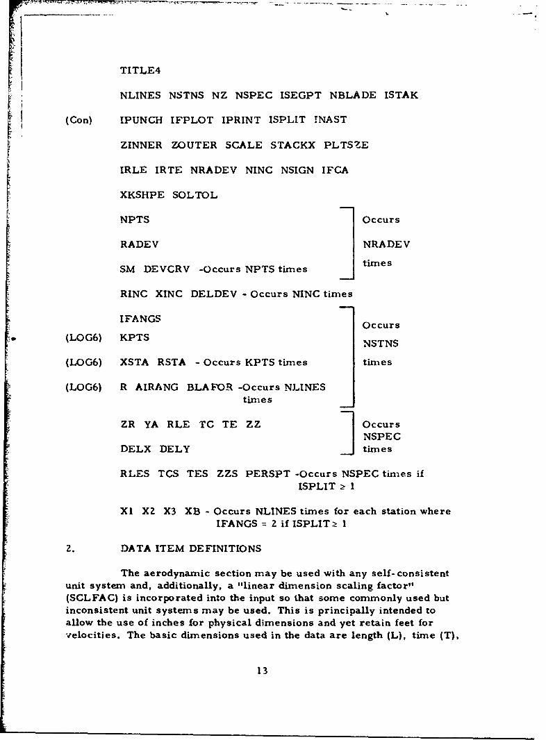
TITLE4

NLINES NSTNS NZ NSPEC ISEGPT NBLADE ISTAK

(Con) IPUNCH IFPLOT IPRINT ISPLIT INAST

ZINNER ZOUTER SCALE STACKX PLTSZE

IRLE IRTE NRADEV NINC NSIGN IFCA

XKSHPE SOLTOL

NPTS Occurs

RADEV NRADEV

SM DEVCRV -Occurs NPTS times J times

RINC XINC DELDEV - Occurs NINC times

IFANGS Occurs

(LOG6) KPTS NSTNS

(LOG6) XSTA RSTA - Occurs KPTS times times

(LOG6) R AIRANG BLAFOR -Occurs NLINEStimes

ZR YA RLE TC TE ZZ OccursNSPEC

DELX DELY times

RLES TCS TES ZZS PERSPT -Occurs NSPEC times ifISPLIT 2 1

XI X2 X3 XB - Occurs NLINES times for each station where

IFANGS = 2 if ISPLITŽ I

2. DATA ITEM DEFINITIONS

The aerodynamic section may be used with any self-consistentunit system and, additionally, a "linear dimension scaling factor"(SCLFAC) is incorporated into the input so that some commonly used butinconsistent unit systems may be used. This is principally intended toallow the use of inches for physical dimensions and yet retain feet for

velocities. The basic dimensions used in the data are length (L), time (T),

13

I , -- -

and force (F). Angles are expressed in degrees (A), and temperatures onan absolute temperature scale (D). Heat capacities (H) are also required.Some possible unit systems are given below, together with the corres-

ponding value of SCLFAC.

L T F D H SCLFAC

Feet Seconds Pounds Deg. Rankine BTU 1.0Inches Seconds Pounds Deg. Rankine BTU 12.0Metres Se,'ivnls Kilograms Deg. Kelvin CHU 1.0

Note t;- i some data names are used in more than one section; careshould be take. co consult the correct sub-division below for definitions.

a. Initial Directives

TITLEl This is a title card for the run.

NANAL The number of blades to be generated by analytic mean-line blade section.

NAERO If NAERO = 0, the aerodynamic section will not beentered.

If NAERO = 1, the aerodynamic section will be entered.

NARBIT The nunmber of blades to be generated by the arbitrarymeanline biade section.

b. Analytic Meanline Blade Section

For a more detailec discussion of the input to this sectionthrough item XB, see References 3 and 5. For this section, the dimen-

sioned input is either in degrees (A) or in length (L).

TITLEZ A title ca-d for the analytic meanline section of theprogram.

NLINES rhe number of strean-,surfaces which are defined, andon which blade sections will be designed. Must satisfy

2 < NLINES - 21.

NSTNS The number of computing stations at which the streanm-surface radii are specified. Must satisfy 3• NSTNS s 10.

NZ The nunmber of constant-z planes on which manufacturing(Cartesian) coordinates for the blade are required. Mustsatisfy 3 • NZ •< 15.

14

NSPEC The number of radially disposed points at which the

parameters of the blade sections are specified. Mustsatisfy I < NSPEC < Zl.

NPOINT The number of points that will be generated to specifythe pressure and suction surfaces of each blade section.Must satisfy 2 < NPOINr < 80. Generally, no less than30 should be used. It will be advantageous to specify 80points when precision plots of the sections are to beproduced directly by the program.

NBLADE The number of blades in the blade row.

ISTAK If ISTAK = 0, the blade will be stacked at the leadingedge.

If ISTAK = 1, the blade will be stacked at the trailingedge.

If ISTAK = 2, the blade will be stacked at, or offset"from, the section centroid.

IPUNCH If the data for subsequent aerodynamic analysis arecomputed (IFANGS = 1), they will also be punched out ifIPUNCH = 1. If not required, set IPUNCH to zero.

ISECN If ISECN = 0, the blade will be constructed using thepolynomial camber line and the standard (i. e. , double-cubic) thickness distribution.

If ISECN = 1, the exponential camber line and thestandard thickness distribution will be used.

If ISECN = 2, the circular arc camber line and the double-circular-arc thickness distribution will be used.

If ISECN = 3, the multiple-circular-arc meanline and thestandard thickness distribution will be ised.

IFCORD If IFCORD = 0, the meridional projections of the stream-surface blade section chords are specified.

If IFCORD = 1, the stream surface blade section chordsare specified.

15

IFPLOT Where CALCOMP software is incorporated into thecomputing system, IFPLOT specifies the creation ofprecision plots. (Further information regarding therequirements for this are given in the section entitled"Program Operation and Structure. ")

If IFPLOT = 0, no plots will be produced.

If IFPLOT = 1, a plot of the streamsurface sections willbe produced. All NLINES sections are shown super-imposed. The origin for each section plot is offsetfrom the centroid of the section by distances specifiedby DELX and DELY.

If IFPLOT = 2, a plot uf tht manufacturing sections willbe produced. The origin is the blade stacking axis, andall NZ sections are shown superimposed.

If IFPLOT = 3, both of the plots described for IFPLOT1 and 2 will be produced.

If IFPLOT = 4, individual plots of each of the manu-

facturing sections will be produced. The axes arerotated clockwise by the section stagger angle for eachplot, so that a large scale may be used.

IPRINT The input data is always listed by the program. Detailsof the stream surface and manufacturing sections areprinted as prescribed by IPRINT.

If IPRINT = 0, details of streanmsurface and manufacturingsections are printed.

If IPRINT = 1, details of stream surface sections *eprinted.

If IPRINT = 2, details of manufacturing sections areprinted.

If IPRINT = 3, details of neither stream surface normanufacturing sections are printed. (The interface datafor use with the aerodynamic section of the program isstill displayed.)

16

ISPLIT If ISPLIT - 0, principal (that is, conventional) bladesare to br! designed.

If ISPLIT - 1, splitter blades having the standard thick-ness distribution are to be designed.

If ISPLIT = 2, splitter blades having the DCA thicknessdistribution are to be designed.

INAST If INAST = 0, no NASTRAN--compatible data is generated.

If IINAST I = 3, NASTRAN-compatible data is generatedusing three-point averages.

If INAST 4, NASTRAN-compatible data is generatedusing four-point averages.

If INAST is positive, both geometric and pressure-loaddata -re output.

If INAST is negative, the pressure-load data is not out-put, and will have to be generated elsewhere, such asby the aerodynamic section.

See the Output Data description (Section IV, 1) for furtherdetails.

IRLE The computing station number at the blade leading edge.

IRTE The computing station number at the blade trailing edge.

NSIGN Jndicator used to sign blade pressure forces accordingto program sign conventions. For compressor rotors,if the machine rotates clockwise when viewed from thefront, set NSIGN to 1; otherwise, set NSIGN to -1.For compressor stators, the two values given forNSIGN are reversed.

ZINNER, The NZ manufacturing sections are equi-spaced betweenZOUTER z equals ZINNER and ZOUTER.

SCALE When precision plot.s are produced, SCALE is the scalefactor employed.

17

STACKX This is the axial coordinate of the stacking axis for theblade, relative to the same origin as used for thestation locations, XSTA.

PLTSZE The size (inches) of the plotter to be used in the creationof precision plots.

KPTS The number of points provided to specify the shape of acomputing station.

If KPTS = 1, the computing station is upright and linea&.

If KPTS = 2, the computing station is linear and eitherupright or inclined.

If KPTS > 2, a spline curve is fit through the pointsprovided to specify the shape of the station.

IFANGS If IFANGS = 0, the calculations of the quantities requiredfor aerodynamic analysis will be omitted at a particularcomputing station.

If IFANGS = 1, these calculations will be performed atthat station.

XSTA An array of KPTS axial coordinates (relative to an arbi-trary origin) which, together with RSTA, specify theshape of a particular computing station.

RSTA An array of KPTS radii which, together with XSTA,specify the shape of a particular computing station.

R The stream surface radii at NLINES locations at each ofthe NSTNS stations.

BLAFOR The difference in pressure between points on the bladepressure surface and suction surface. If zero is input,the output generated for the NASTRAN program willreflect no aerodynamic loading. The pressure differenceshould be in units of force per length squared, wherelength is the s.-ie unit as the dimensions of the bladeunder consideration

18

ZR The variation of properties of the streamsurface bladesection is specified as a function of strearnsurfacenumber. The various quantities are then interpolated

t (or extrapolated) at each streamsurface. The stream-surfaces are numbered consecutively from the inner-most outward, starting with 1. 0. ZR must increasemonotonically, there being NSPEC values in all.

BI The blade irlet angle.

B2 The blade outlet angle.

PP If ISECN = 0, PP is the ratio of the second derivative ofthe camber line at the leading edge to its maximum value.Must satisfy -2.0 < PP< 1.0.

If ISECN = 1, PP is the ratio of the second derivative ofthe camber line at the leading edge to its n aximum valueforward of the inflection point. Must satisfy 0. 0 < PP ! 1. 0.

If ISECN = 2 or 3, PP is superfluous.

QQ If ISECN = 0, QQ is the ratio of the second derivative ofthe camber line at the trailing edge to its maximum value.Must satisiy 0.0 < QQ T 1.0.

If ISECN = 1, QQ is the ratio of the second derivative ofthe camber line at the trailing edge to its maximum valuerearward of the inflection point. Must satisfy 0. 0 < QQ< 1.0.

If ISECN = 2 or 3, QQ is superfluous.

RLE The ratio of blade leading edge radius to chord.

TC The ratio of blade maximunm thickness to chord.

TE The ratio of blade trailing edge half-thickness to chord.

If ISECN = 2, TE is superfluous.

Z The location of the blade maximum thickness, as a fractionof camber line length from the leading edge.

If ISEGN = 2, Z is superfluous.

19

CORD If IFCORD 0, CORD is the meridional projcction of theblade chord.

If IFCORD 1, CORD is the blade chord.

DELX, The stacking axis passes through the stream surface bladeDELY sections, offset from the centroids, leading, or tra.ling

edge by DELX and DELY i,j the x and y directionsrespectively.

S, BS If ISECN = 1 or 3, S and BS are used to specify thelocations of the inflection point (as a fraction of the

meridionally-projected chord length) and the change incamber angle from the leading edge to the inflection point.If the absolute value of the angle at the inflection pointis larger than the absolute value of BI, BS should have

the same sign as BI, otherwise, BI and BS should be

of opposite sign.

RLES The ratio of splitter section leading edge radius to

splitter chord.

TCS The ratio of splitter section maximum thickness to

splitter chord.

TES The ratio of splitter section trailing-edge half-thicknes:to splitter chord. If ISPLIT = 2, this item is super-

fluous.

ZZS The location of the splitter section maximum thickness,as a fraction of splitter camber line length. If ISPLIT ;2, this item is superfluous.

PERSPT The ratio of desired splitter axial chord to main bladeaxial chord on the particular stream surface.

XI, X2, X3 These quantities are not :-ead. They may be left blank.

XB The blockage due to the principal blades that is to beadded to that computed for the splitter blades. (Generally,

cards containing these data in the correct format will have

been produced by use of the IFANGS = 1 and IPUNCH = Ioptions when computing the principal blades. Take careonly tV incorporate those cards that correspond to

locations within the splitter blade envelope.)

20

NRAD The number of radii at which a distribution of thefraction of trailing edge deviation is input. Mustsatisfy 1 • NRAD < 5.

NDPTS I .e number of points used to define each deviation curve.Must satisfy I • NDPTS: 11.

NDATR The number of radii at which an additional deviation angleincrement and the point of maximum camber arespecified. Must satisfy 1 < NDATR r 21.

NSWITC If NSWITC = 1, the deviation correlation parameter "m"for the NACA (A 1 0 ) meanline is used.

If NSWITC = 2, the deviation correlation parameter "Im"

for double-circular-arc blades is used.

NLE Station number at leading edge.

NTE Station number at trailing edge.

XKSHPE The blade shape correction factor in the deviation rule.

SPEED See definition for Aerodynamic Section.

NR The number of radii where a "loss" is input.

NTERP

NMACH

NLOSS

NLI

NL2

NEVAL

NCURVE See definition for Aerodynamic Section.

NLITER

NDEL

NOUTI

NOUT2

NOUT3

NBLAD IR Radius at which loss is specified.

21

XLOSS Loss description. The form is prescribed by NLOSS;see aerodynamic section.

RTE Radius at blade trailing edge where the following deviationfraction/chord curve applies.

If NRAD = 1, it has no significance. Must increasemonotonically.

DM The location on the meridional chord where the deviationfraction is given. Expressed as a fraction of themeridional chord from the leading 3dge. Must increasemonotonically.

DVFRAC Fraction of trailing -edge deviation that occurs at locationDM.

RDTE Radius at trailing edge where additional deviation andpoint of maximum camber are specified.

DELTAD Additional deviation angle added to that determined bydeviation rule. Input positive for conventionally positivedeviation for both rotors and stators.

AC Fraction of blade chord from leading edge where maximumcamber occurs.

c. Aerodynamic Section

TITLE3 A title card for the aerodynamic section of the program.

CP Specific heat at constant pressure. An input value ofzero will be reset to 0. 24. Units: H/F/D.

GASR Gas constant. An input value of zero will be reset to53.32. Units: L/SCLFAC/D.

G Acceleration due to gravity. An input value of zero willbe reset to 32. 174. Units: L/SCLFAC/T/T.

EJ Joules equivalent. An input value of zcro will be resetto 778.16. Units: LF/SCLFAC/H.

NSTNS Number of computing stations. Must satisfy 3 s NSTNSS30.

22

NSTRMS Nuriber of streanilineu. Must satisfy 3 < NSTRMS • 21.

An .nput value of zero will be reset to II.

NMAX Maxin.um number of passes through the iterative stream-line determination procedure. An input value of zero will

be reset to 40.

NFORCE The first NFORCE passes are performed with arbitrarynumbers inserted should any calculation produceimpossible values. Thereafter, execution will cease,

the calculation having "failed". An input value of zerowill be reset to 10.

NBL If NBL ý 0, the annulus wall boundary layer blockageallowance will be held at the values prescribed byWBLOCK.

If NBL = 1, blockage due to annulus wall boundary layerswill be recalculated except at station 1. VISK and

SHAPE are used in the calculation.

NGASE Number of speed/flow combinations to be computed.Must satisfy I < NCASEs 10, except that an input valueof zero will be reset to 1.

NSPLIT If NSPLIT = 0, the flow distribution between the stream-lines will be determined by the program so that roughlyuniform increments of computing station will occurbetween the streamlines at station 1.

If NSPLIT = 1, the flow distribution between the stream-lines is read in (see DELF).

NSET1 The blade loss coefficient re-evaluation option (specifiedby NEVAL) requires loss parameter/diffusion factordata. NSET1 sets of data are input, the set numbers beingallocated according to the order in which they are input.Up to 4 sets may be input (see NDIFF).

NSET2 When NLOSS = 4, the loss coefficients at the station aredetermined as a fraction of the value at the trailing edge.Then, NSET2 sets of curves are input to define thisfraction at a function of radius and nieridional chord. Upto 2 sets may be input (see NM).

23

NREAD If NREAD 0, the initial streamline pattern estimateis generated by the program.

If NREAD = 1, the initial streamiiline pattern estimate andalso the DELF values are read in. (See DELF, R, X,XL. )

NPUNCH If NPUNCH = 0, no action is taken.

If NPUNCH = 1, the final streamline pattern computedfor each running point calculationa that did not fail willbe punched. The DELF values are also punched.

NPLOT If NPLOT = 0, no action is taken.

If NPLOT = 1, a CALCOMP plot of the static pressuredistributions on hub, mid, and tip streamlines will bemade for each point.

If NPLOT = 2, a CALCOMP plot of the final streamlinepattern will be made for each point.

If NPLOT = 3, the plots made for NPLOT = I and 2 willboth be macle. (See XSCALE, PSCALE, RLOW, PLOW.)

NPAGE The maximum number of lines printed per page. Aninput value of zero will be reset to 80.

NTRANS If NTRANS = 0, no action is taken.

If NTRANS = 1, relative total pressure loss coefficientswill be modified to account for radial transfer of wakes.See Section V. 11.

NMIX If NMIX = 0, no action is taken.

If NMIX = 1, entropy, angular momentunm, and totalenthalpy distributions will be modified to account forturbulent mixing. See Section V. 12.

NMANY The number of computing stations for which bladedescriptive data is being generated by the analytic mean-line section.

Z4

NSTPLT If NSTPLT = 0, no action is taken.

If NSTPLT = 1, a line-printer plot of the changes madeto the midstreamline T coordinate is made for eachcomputing station. If more than 59 passes through theiterative procedure have been made, then the plots willshow the changes for the last 59 passes. The graphshould decay approximately exponentially towards zero,indicating that the streamline locations are stabilizing.Decaying oscillations are equally acceptable, but, growingoscillations show the need for heavier damping in thestreamline relocation calculations, that is, a decrease

in RCONST.

NEON This item controls the selection of the form of momentumequation that will be used to compute the meridionalvelocity distribution at each computing station. There aretwo basic forms, and for each case, one may select notto compute the tern.s relating to blade forces. (See alsoSection V. 1.)

If NEON = 0, the momentum equation involves the differ-ential form of the continuity equations and hence (0- Mterms in the denominator. Streamwise gradients ofentropy and angular momentum (blade forces) are con-puted within blades and at the blade edges (provided datathat describe the blades are given). Elsewhere, stream-wise entropy gradients only are included in a sin.pler formof the monsentum equation, except that at the first and lastcomputing station, all streamwise gradients are taken tobe zero. This is generally the preferred option whencomputing stations are located within the blade rows.

If NEON = 1, the momentum, equation form is similar tothat used when NEON = 0, but angular momentun, gradients(blade force terms) are nowhere computed. This generall)is the preferred option when computing stations are locatedat the blade edges only.

If NEON = Z, the momentum equation includes an explicitdVm 1dm term instead of the (I- ti) denominator terms.

All streanwise gradients (including blade force terms)are computed as for the case NEON = 0. When computingstations are located within the blade rows, the resultswill generally be similar to those obtained with NEON = 0.and solutions may be found that cannot be computed with

NEON = 0 due to high meridional Mach numbers.

25

IIf NEQN = 3, the momentum equation is similar to thatused when NEQN = 1, but (as for the case NEQN = 1) noangular momentum gradients are computed. This may beused when computing stations are located only at the bladeedges and high meridional Mach numbers preclude theuse of NEQN = 1.

NWHICH The numbers of each of the computing stations for whichblade descriptive data is being generated by the analyticmeanline section.

SCLFAC Linear dimension scale factor. An input value of zerowill be reset to 12.0.

TOLNCE Basic tolerance in iterative calculation scheme. An inputvalue of zero will be reset to 0. 001. (See discussion oftolerance scherme in Section VI.)

VISK Kinematic viscosity of gas (for annulus wall boundarylayer calculations). An input value of zero will be reset

to 0.00018. Units: LL/SCLFAC/SCLFAC/T.

SHAPE Shape factor for annulus wall boundary layer calculations.An input value of zero will be reset to 0. 7.

XSCALE The scale used for the physical dimensions in the staticpressure and streamline plots given as length unit perinch of plot.

PSCALE The scale used to plot static pressure given as pressureunit per inch of plot.

RLOW Mininmum value of radius shown on streamline plots.Units: L.

PLOW Minimum value of pressure shown on static pressureplots. Units: F/L/L.

XMMAX The square of the Mach number that appears in the equationfor the streamline relocation relaxation factor is limitedto be not greater than XMMAX. Thus, at computing sta-tions where the appropriate Mach number is high enoughfor the limit to be imposed, a decrease in XMMAXcorresponds to an increase in damping. If a value of zerois input, it is reset to 0. 6.

26

-17~~- -7 -_ :

RCONST The constant in the equation for the streamline relocationrelaxation factor. The value of 8. 0 that the analysis yieldsis often too high for stability. If zero is input, it is resetto 6.0.

CONTR The constant in the blade wake radial transfer calculations.

C•ONMX The eddy viscosity for the turbulent mixing calculations.Units: L 2 /SCLFAC 2 /T.

FLOW Compressor flow rate. Units: F/T.

SPDFAC The speed of rotation of each computing station is SPDFACtimes SPEED (I). The units for the product are revolutions/(60xT).

NSPEC The number of points used to define a computing station.Must satisfy 2 < NSPEC - 21, and also the sum of NSPECfor all stations ! 150. If 2 points are used, the station isa straight line. Otherwise, a spline-curve is fittedthrough the given points.

XSTN, RSTN The axial and radial coordinates, respectively, of a pointdefining a computing station. The first point must be onthe hub and the last point must be on the casing. Units: L.

NDATA Number of points defining conditions or blade geometry ata computing station. Must satisfy 0 : NDATA • 21, andalso the sum of NDATA for all stations < 100.

NTERP If NTERP = 0, and NDATA Ž 3, interpolation of the dataat the station is by spline-fit.

If NTERP = 1 (or NDATA -f 2), interpolation is linear_ I point-to -point.

NDIMEN If NDIMEN = 0, the data are input as a function of radius.

If NDIMEN = 1, the data are input as a function of radiusnormalized with respect to tip radius.

If NDIMEN = 2, the data are input as a function of distancealong the computing station from the hub.

27

If NDIMEN = 3,. the data are input as a function ofdistance along the computing station normalized withrespect to the total computing station length.

NMACH If NMACH = 0, the subsonic solution to the continuityequation is sought.

If NMA CH = 1, the supersonic solution to the continuityequation is sought. This should only be used at stationswhere the relative flow angle is specified, that is,NWORK = 5, 6, or 7.

DATAC The coordinate on the computing station, defined accordingto NDIMEN, where the following data items apply. Must

increase n.onotonically. For dimensional cases, units areL.

DATAI At Station I and if NWORK = 1, DATAI is total pressure.Units: F/L/L.

If NWORK = 0 and the station is at a blade leading edge,by setting NDATA =' 0, the blade leading edge may bedescribed. Then DATA I is the blade angle measured inthe cylindrical plane. Generally negative for a rotor,positive for a stator. (Define the blade lean angle (DATA3)

also.) Units: A.

If NWORK = 2, DATAI is total enthalpy. Units: H/F.

If NWORK = 3, DATA1 is angular momentum (ra,'4ius tin.esabsolute whirl velocity). Units: LL/SCLFAC/T.

If NWORK = 4, DATAI is absolute whirl velocity. Units:L/SCLFAC/T.

If NWORK = 5, DATA I is blade angle measured ip thestrean.surface plane. Generally negative for a rotor,positive for a stator. If zero deviation is input, it"becomesthe relative flow angle. Units: A.

If NWORK = 6, DATAI is the blade angle measured in thecylindrical plane. Gererally negative for a rotor, positivefor a stator. If zero deviation is input, it becomes, aftercorrection for stream surface orientation and station leanangle, the relative flow angle. Units: A.

28

If NWORK = 7, DATA I is the reference relative outletflow angle measured in the streaan;surface plane. Generallynegative for a rotor, positive for a stator. Units: A.

DATA2 At Station 1, DATA2 is total temperature. Units: D.

If NLOSS = 1, DATA2 is the relative total pressure losscoefficient. The relative total pressure loss is measuredfrom the station that is NLI stations removed from thecurrent station, NLl being negative to indicate anupstream station. The relative dynamic head is determinedNLZ stations removed from the current station, positivefor a downstream station, negativv for an upstream station.

If NLOSS = 2, DATA2 is the isentropic efficiency ofcompression relative to condition- NLI stations removed,NL1 being negative to indicate an upstream station.

If NLOSS = 3, DATAZ is the entropy rise relative to thevalue NLI stations removed, NLI being negative toindicate an upstream station. Units: H/F/D.

If NLOSS = 4, DATAZ is not used, but a relative totalpressure loss coefficient is determined from the trailingedge value and curve set number NGURVE of the NSET2families of curves. NLI and NL2 apply as for NLOSS = 1.

If NWORK = 7, DATA 2 is the reference (mininmum)relative total pressure loss coefficient. NLI and NL2apply as for NLOSS = 1.

DATA3 The blade lean angle measured from the projection of aradial line in the plane of the computing station, positivewhen the innermost portion of the blade precedes theoutermost in the direction of rotor rotation. Units: A.

DATA4 The fraction of the periphery that is blocked by the presenceof the blades.

DATA5 Cascade solidity. When a number of stations are used todescribe the flow through a blade, values are only requiredat the trailing edge. (They are used in the loss coefficientre-estimation procedure, and to evaluate diffusion factorsfor the output.)

29

DATA6 If NWORK = 5 or 6, DATA6 is the deviation anglemeasured in the streamsurface plane. Generally negativefor a rotor, positive for a stator. Units: A.

If NWORK = 7, DATA6 is reference relative inlet angle,to which the minimum loss coefficient (DATAZ) and thereference relative outlet angle (DATA7) correspond.Measured in the streamsurface plane and generallynegative for a rotor, positive for a stator. Units: A.

DATA7 If NWORK = 7, DATA7 is the rate of change of relativeoutlet angle with relative inlet angle.

DATA8 If NWORK = 7, DATA8 is the relative inlet angle largerthan the reference value at which the loss coefficient attainstwice its reference value. Measured in the streamnsurfaceplane. Units: A.

DATA9 If NWORK = 7, DATA9 is the relative inlet angle smallerthan the reference value at which the loss coefficient attainstwice its reference value. Measured in the stream surfaceplane. Units: A.

NWORK If NWORK = 0, constant entropy, angular momentum, andtotal enthalpy exist along streamlines from the previousstation. (If NMIX = 1, the distributions will be modified.)

If NWORK = 1, the total pressure distribution at the com-puting station is specified. Use for rotors only.

If NWORK = 2, the total enthalpy distribution at the com-puting station is specified. Use for rotors only.

If NWORK = 3, the absolute angular momentum distributionat the z!cnu,,ting station is specified.

If 74WORK = 4, the absolute whirl velocity distribution atthe computing station is specified.

If NW)RK = 5, the relative flow angle distribution at thestation is specified by giving blade angles and deviationangleF, both measured in the streanmsurface plane.

If NWORK = 6, the relative flow angle distribution at thestation is specified by giving the blade angles measuredin the cylindrical plane, and the deviation angles measuredin the stream surface plane.

30

If NWORK 7, the relative flow angle and relative totalpressure loss coefficient distributions are specified bymeans of an off-design analysis procedure. "Reference","stalling", and "choking" relative inlet angles arespecified. The minimunm loss coefficient varies para-bolically with the relative inlet angle so that it is twicethe minirruni value at the "stalling" or "choking" values.A maximum value of 0. 5 is imposed. "Reference"relative outlet angles and the rate of change of outletangle with inlet angle are specified, and the relative

outlet angle varies linearly irom the reference valuewith the relative inlet angle. NLOSS should be set to zero.

NLOSS I' :LOSS = 1, the relative total pressure loss coefficientdi•.tribution is specified.

If NLOSS = 2, the isentropic efficiency (for compression)distribution is specified.

If NLOSS = 3, the entropy rise distribution is specified.

If NLOSS = 4, the total pressure loss coefficient distribution

is specified by use of curve-set NCURVE of the NSETZfamilies of curves giving the fraction of final (trailingedge) loss coefficient.

NL1 The station fron, which the loss(in whatever form NLOSSspecifies) is measured, is NL1 stations removed from thestation being evaluated. NLI is negative to indicate an

upstream station.

NL2 When a relative total pressure loss coefficient is used tospecify losses, the relative dynamic head is taken NL2stations removed from the station being evaluated. NL2may be positive, zero, or negative; a positive valueindicates a downstream station, a negative value indicates

an upstream station.

NEVAL If NEVAL = 0, no action is taken.

If NEVAL >0, curve-set number NEVAL of the NSETIfamilies of curve giving diffusion loss parameter as afunction of diffusion factor will be used to re-estimiatethe relative total pressure loss coefficient. NLOSS must

be 1, and NLI and NL2 must specify the leading edge ofthe blade. See also NDEL.

31

If NEVAL <0, curve-set number I NEVAL I is used

NEVAL > 0, except that the re-estimation is only ma-eafter the overall computation is completed (with the inputlosses). The resulting loss coefficients are displayed but

not incorporated into the overall calculation. See alsoNDEL.

NCURVE When NLOSS = 4, curve-set NCURVE of the NSETZfamilies of curves, specifying the fraction of trailing-edge loss coefficient as a function of meridional chord

is used.

NLITER When NEVAL > 0, up to NLITER re-estimations of the losscoefficient will be n.ade at a given station during any onepass through the overall iterative procedure. Less than

NLITER re-estimations will be made if the velocityprofile is unchanged by re-estimating the loss coefficints.

(See discussion of tolerance scheme in Section VI.)

NDEL When NEVAL = 0, set NDEL to 0. When NEVAL / 0, and= I NDEL > 0, a component of the re-estinmated loss coefficient

is a shock loss. The relative inlet Mach number is

expanded (or compressed) through a Prandtl-Meyerexpansion on the suction surface, and NDEL is the numberof points at which the Prandtl-Meyer angle is given. If

NDEL = 0, the shock loss is set to zero. Must satisfyo • : NDEL - 21, and also the sunm of NDEL for all stations

ý5 100.

NOUTI If NOUTI = 0, no action is taken.

If NOUTI 1, cards will be punched that may be incorporatedinto the data deck for a subsequent run of Uhe analytic mean-line section. These a:e the (NLINES times NSTNS) cardsspecifying R.

NOUTZ If NOUTZ = 0, no action is taken.

If NOUT2 = 1, output records are created that nay be usedas input to the arbitrary meanline section. These arerecords specifying KPTS, XSTA, RSTA, R, and AIRANG.

If NARBIT = 0, the records will be issued is punch cards;If NARBIT = 1, the records will be stored within thecomputer on file LOG6.

32

NOUT, This data :zern controls the generat:on of NASTRAN-cornpatib] _ pressure difference output for use in asubseque-* blade stress analysis. For details of thetriangular mesh that is used, see the Output Descriptionin Section IV. 2. c.

If NOUT3 = 1, the station is at a blade leading edge.

If NOUT3 = 2, the station is at a blade trailing edge.

If NOUT3 = 3, the station is at the trailing edge of oneblade, and at the leading edge of another.

If NOUT3 = 0, the station may be between blade rows,or within a blade row for which output is required,depending upon the use of NOUT3 4 0 elsewhere. Seealso description of NBLADE below.

NBLADE This item is used in determining the pressure differenceacross the blade. The number of blades is I NBLADE !"If NBLADE is positive, "three-point averaging" is usedto determine the pressure difference across each bladeelement. If NBLADE is negative, "four-point averaging"is used. (See the Output Description in Section IV. 2. c.)If NBLADE is input as zero, a value of +10 is used. Ata leading edge, the value for the following station is used:elsewhere the value at a station applies to the interv, 1upstream of the station. Thus by varying the -ign ofNBLADE, the averaging method used for the pressure forcesmay be varied for different axial segments of a blade row.

SPEED This card is omitted if NDATA = 0. The speed of rotationof the blade. At a blade leading edge, it should be set tozero. The product SPDFAC times SPEED has units ofrevolutions/( T x 60).

DELC The coordinate at which Prandtl-Meyer expansion anglesare given. It defines the angle as a function of thedimaensions of the leading edge station, in the mannerspecified by NDIMEN for the current, that is trailingedge station. Must increase monotonically. For dimen-sional cases, units are L.

33

DELTA The Prandtl-Meyer expansion angles. A positive valueimplies expansion. If blade angles are given at the leadingedge, the incidence angles are added to the value specifiedby DELTA. Units: A. (Blade angles are measured inthe cylindrical plane.)

WBLOCK A blockage factor that is incorporated into the continuityequation to account for annulus wall boundary layers. Itie :xpressed as the fraction of total area at the computingstation that is blocked. If NBL = 1, values (except atStation 1) are revised during computation, involving dataitems VISK and SHAPE.

BBLOCK, A blockage factor is incorporated into the continuityBDIST equation that may be used to account for blade wakes or

other effects. It varies linearly with distance along thecomputing station. EBLOCK is the value at mid-station(expressed as the fraction of the periphery blocked), andBDIST is the ratio of the value on the hub to the mid-value.

NDIFF When NSETI> 0, there are NDIFF points defining lossdiffusion parameter as a function of diffusion factor.Must satisfy 1 • NDIFF • 15.

DIFF The diffusion factor at which loss parameters are specified.Must increase monotonically.

FDHUB Diffusion loss parameter at 10 per cent of the radial bladeheight.

FDMID Diffusion loss parameter at 50 per cent of the radial bladeheight.

FDTIP Diffusion loss parameter at 90 per cent of the radial bladeheight.

NM When NSETZ-2. 0, there are NM points defining the fractionof trailing edge loss coefficient as a function of meridionalchord. Must satisfy I - NM • 11.

NRAD The number of radial locations where NM loss fraction/chord points are given. Must satisfy 1 • NRAD , 5.

_)4

TERAD The fraction of radial blade height at the trailing edgewhere the following loss fraction/chord curve applies.If NRAD = 1, it has no significance.

DM The location on the meridional chord where the lossfraction is given. Expressed as a fraction of meridionalcho-rd from the leading edge. Must increase mono-tonically.

WFRAC Fraction of trailing edge loss coefficient that occurs atlocation DM.

DELF The fraction of the total flow that is to occur between thehub and each streamline. The hub and casing are included,so that the first value must be 0. 0, and the last (NETRM)value must be 1. 0.

R Estimated streamline radius. (These data are input fromhub to tip for the first station, from hub to tip for thesecond station, and so on.) Units: L.

X Estimated axial coordinate at intersection of streamlinewith computing station. Units: L.

XL Estimated "1istance along computing station from hub tointersection of streamline with computing station.Units: L.

II, JJ Station ,,nd streamline number. These are merely readin and printed out to give a check or th,: order of the cards,presumed to have been punched on p- evious run.

d. Arbitrary Meanline BlaA( :-ection

For a more detailed discussion of the input tr. this section, seeReference 4. In this section, the dimensioned input is either in degrees(A), or length (L).

TITLE4 A title card for the arbitrary meanline section of theprogram.

NLINES As for Analytic Meanline Section.

NSTNS As for Analytic Meanline Section.

NZ As for Analytic Meanline Section.

35

NSPEC As for Analytic Meanline Section.

ISEGPT The number of points to define each surface in each blade

segment, including the end-points common to the adjacentsegments. Must satisfy 2•ISEGPT and also (ISEGPT-1)

times the number of segments ! RO. (The number of

segments is IRTE - IRLE + I.)

NBLADE As for Analytic Meanline Section.

ISTAK As for Analytic Meanline Section.

IPUNCH As for Analytic Meanline Section.

IFPLOT As for Analytic Meanline Section.

IPRINT As for Analytic Meanline Section.

INAST As for Analytic Meanline Section.

ZINNER As for Analytic Meanline Section.

ZOUTER As for Analytic Meanline Section.

SCALE As for Analytic Meanline Section.

STACKX As for Analytic Meanline Section.

PLTSZE As for Analytic Meanline Section.

IRLE Station number at blade leading edge. Note that the firststation specified it..ne arbitrary meanline section is

number 1.

IRTE Station number at blade trailing edge.

NRADEV The number of radii at which a distribution of the fractionof trailing edge deviation is inp'.. Must satisfy

1 < NRADEV:• 5.

NINC The number of radii at which the incidence angle is

specified. Must satisfy I < NINC • 5.

NSIGN This is used to establish the sign convention. Normally,+ I for stators and -I for rotors.

36

4

IFCA If IFCA = 1, the deviation correlation parameter "ni"for the NACA (A 1 o) meanline is used.

If IFCA - 2. the deviation correlation parameter "Im"

for double-circular-arc blades is used.

XKSHPE The blade shape correction factor in the deviation rule.

SOLTOL Solidity tolerance in iteration for deviation angle.

NPTS The number of points defining the deviation curve.

RADEV Radius at the blade ti'ailing-edge where the followingdeviation fraction/chord curve applies. If NRADEV = 1.it %as no significance. Must increase mionotonically.

SlMI T'he location on the meridional chord where the deviationfraction "s given. Expressed as a fraction of the meridional

chord from the leading edge. Must increase monotonically.

DEVCRV Fraction of trailing-edge deviation that occurs at locationsm.

RINC Radius at which incidence angle and additional deviationangle is given.

XINC Incidence angle at radius RINC. Input positive for conven-

tionally-positive incidence for both rotors and stators.

DELDEV Additional deviation angle added to that determined bydeviation rule. Input positive for conventionally positivedeviation for both rotors and stators. Applied on thestreanrsurface that passes through the leading edgestation at radius RINC.

IFANGS As for Analytic Meanline Section.

XPTS As for Analytic Meanline Section.

XSTA As for Analytic Meanline Section.

RSTA As for Analytic Nleanline Section.

R Streamnsurface radius.

37

AIRANG Relative flow angle at radius R. Normally negative forrotors, positive for stators.

BLA MR As for Analytic Meanline Section.

ZR The variations of properties of the stream surface bladesections are specified as a function of stream surfacenumber. The streamsurfaces are numbered consecutivelyfrom the innermost outward. Iviust increase monotonically.

YA The chord is multiplied by the factor (1-YA) when thesolidity is determined, which is then used in the deviationangle calculations.

RLE The ratio of blade leading-edge radius to the chord.

TC The ratio of blade maximum thickness to chord.

TE The ratio of blade trailing-edge half-thickness to chord.

ZZ The point of blade nmaximum thickness, as a fraction ofcamber line length from the leading edge.

DELX, As for Analytic Meanline Section.DELY

Xl, X2 As for Analytic Meanline Section.X3, XB

38

ISECTION IV

OUTPUT DATA

1. ANALYTIC MEANLINE SECTION

Printed output may be considered to consist of four sections; a print-out of the input data, details of the blade sections on each streamrsurface, alisting of quantities required for aerodynamic analysis, and details of themanufacturing sections determined on the constant-z planes. These arebriefly described below. In the ,.xplanation which follows, parentheticalstatements are understood to refer to the particular case of the double-circular-arc blade (ISECN = 2).

The input data printout includes all quantities read in, and is self-explanatory.

Details of the stream surface blade sections are printed if IPRINT0 or 1. Listed first are the parameters defining the blade section. Theseare interpolated at the stream surface from the tables read in. Then followdetails of the blade section in "nornalized" form. The blade section geometryis given for the section specified, except that the meridional projection ofthe chord is unity. For this section of the output, the coordinate origin isthe blade leading edge. The following quantities are given: blade chord;stagger angle; can ber angle; section area; location of the centroid of thesection; second momen -. of area of the section about the centroid; orienta-tion of the principal axes; and the principal second moments of area rf thesection about the centroid. Then are listed the coordinates of the camberline, the camber line angle, the section thickness, and the coordinates ofthe blade surfaces. NPOINT values are given.

A lineprinter plot of the normalized section follows. The scales forthe plot are arranged so that the section just fills the page, so that the

- scales will generally differ from one plot to another. "Dimensional" detailsof the blade section are given next. The normalized data given previously isscaled to give a blade section as defined by IFCORD and CORD. For thissection of the output, the coordinates are with respect to the blade stackingaxis. The following quantities are given: blade chord; radius and locationof center of leading (and trailing) edge(s); section area, the second momentsof area of the section about the centroid and the principal second momentsof area of the section about the centroid. The coordinates of NPOINT pointson the blade surfaces are then listed, followed by the coordinates of 31points distributed at (roughly) six degree intervals around the leading (andtrailing) edges. Finally, the coordinates of the blade surfaces and pointsaround the leading (and trailing) edge(s) is (are) shown in Cartesian form.

39

The quantities required for aerodynamic analysis are printed at allcomputing stations specified by the IFANGS parameter. The radius, bladesection angle, blade lean angle, blade blockage, and relative angularlocation of the camber line are printed at each stream surface intersectionwith the particular computing station. The blade section angle is measuredin the cylindrical plane, and the blade lean angle is measured in the constant-axial-coordinate plane.

Details of the manufacturing sections are printed if IPRINT = 0 or 2.At each value of z specified by ZINNER, ZOUTER, and NZ, sectionproperties and coordinates are given. The origin for the coordinates is the

blade stacking axis. The following quantities are given: section area; thelocation of the centroid of the section; the second moments of area of thesection about the centroid; the principal second poments of area of thesection about the centroid; the orientation of the principal axes; and thesection torsional constant. Then the coordinates of NPOINT points on theblade section surfaces are listed, followed by 31 points around the leading

(and trailing) edge(s).

If NAERO = 1, the additional input and output required for, andgenerated by, the interface are also printed. (Apart from the input dataprintout, this is the only printed output when IPRINT = 3.)

If IPUNCH =1 and NAERO = 0, the program punches the quantitiesrequired for aerodynamic analysis, together with identifying indices denotingstation number and streamsurface number, on cards in the following format:

5 fields each of 12 locations for the quantities themselves, followed by 2fields each of 3 locations for the indices.

If INAST 40, cards are punched that may be used as input for theNASTRAN stress analysis program. For the purpose of stress analysis,the blade is divided into a number of triangular elements, each defined bythree grid points. The intersections between computing stations andstream surfaces are used as the grid points, and the grid points and elementnumbering scheme adopted through Program UD0300 is illustrated inFigire 1.

The NASTRAN input data format includes cards identified by the codesGRID, CTRIA2, PTRIA2, and PLOAD2. The data are fully described inReference 7, but briefly, the GRID cards each define a grid point num1berand give the coordinates at the grid point, the CTRLAZ cards each define anelement in terms of the three appropriate grid points (by number, and in asignificant order), the PTRIA2 cards each give an average blade thicknessfor an element, and the PLOAD2 cards each give an average pressureloading for an element. If IINAST = 3, the thicknesses and pressures are

40

II

Cc 4 c-j 9!' C.2, -)

kT biu 'iN3S ~

ifT

0

2

Figure 1. NASTRAN Grid Point and Element NumberingScheme.

obtained by averaging the values at the three grid points that comprise theblade element. Because of the different weighting towards the "front"and "rear" of the elements, the averages computed do not always varysensibly, especially near the blade edges, and therefore an alternativeaveraging procedure is also available. When IINAST I = 4, the averagesare formed from values at the four grid points which are rather obviouslyrelated to the blade element. (This is indicated in Figure 1.) Note thatas detailed in tae input data description, if INAST is negative, the PLOAD2cards are not punched.

Precision plots are produced if IFPLOT = 1, 2, 3. or 4 as describedunder the definition of IFPLOT given previously.

41

2. AERODYNAMIC SECTION

a. Regular Printed Output

The input data are first printed out in its entirety, and the resultsfor each running point follow. The output is generally self-explanatory anddefinitions are given here for some derived quantities. Tabular output isgenerally not started on a page unless it can be completed on the same page,according to the maximum number of lines permitted by the input variableNPAGE.

The results of each running point are given under a headinggiving the running point number. Any diagnostics generated during thecalculation will appear first under the heading. (Diagnostics are describedin the following section. ) Then, a station-by-station print out follows foreach station through to the last station, or to the station where the calcu-lation failed, if this occurred. One or more diagnostics will indicate thereason for the failure, in this event. Included in the meshpoint coordinatedata is the distance along the computing station from the hub to the inter-ception of the streamline with the station (L), and the station lean angle(GAMA). Where the radius of curvature of a streamline is shown as zero,the streamline has no curvature. The whirl angle is defined by

=c n0 VV (I)

For stations within a blade, or at a blade trailing edge, a rel-ative total pressure loss coefficient is shown. The loss of relative totalpressure is computed from the station defined by the input variable NLI. Ifa loss coefficient was used in the input for the station (NLOSS = 1 or 4, orNWORK = 7), the input variable NLZ defines the station where the norn.alizingrelative d;-namic head is taken; otherwise, it is taken at the station definedby NL1. If the cascade solidity is given as anything but zero, it is used inthe determination of diffusion factors. The following definition is used:

VLr V Voe.f .S= I- (2)

Inlet conditions (subscript 1) are taken from the stationdefined by the input variable NLI.

42

I

The last term in Equation 2 is multiplied by -I if the bladespeed is greater than zero, or the blade speed is zero and the precedingrotating blade row has negative rotation. This is necessary becauserelative whirl angles are (generally) negative for rotor blades and forstator blades that follow a rotor having "negative" wheel speed. Incidenceand deviation angles are treated in the same way. so that positive andnegative values have their conventional significance for all blades.

If annulus wall boundary layer computations were made (NBL= 1), details are shown for each station. Then, an overall result is given,including a statement of the number of passes that have been performed andwhether the calculation is converged, unconverged, or failed. When thecalculation is unconverged, the number of mesh points where the meridionalvelocity component has not remained constant to within the specified toler-ance (TOLNCE) on the last two passes is shown as IVFAIL. Similarily, thenumber of streamtubes, defined by the hub and each streamline in turn,where the fraction of the flow is not within the same tolerance of the targetvalue is shown as IFFAIL. If these numbers are small, say less than 10%of the maxintunm possible values, the results may generally be used. Other-

wise, the computation should be rerun, either for a greater number ofpasses, or with modified relaxation factor constants. If the punch-4 streamline option (NPUNCH =1) was used, the streamline pattern generatedin the first run may be input into the second run (with NREAD =1), restartingthe calculation essentially where it was terminated and thus effecting asaving in computer time. The default option relaxation constants will gener-ally be satisfactory but may need modification for sonme cases. If insufficientdamping is specified by the constants, the streamlines generated will tendto oscillate and this may be detected by observing a relatively small radiusof curvature for the mid-passage streamline that also changes sign from onestation to the next. This nmay be corrected by rerunning the problem (fromscratch) with a lower value input for RCONST, say, of 4. 0 instead of 6. 0. Whenthe damping is excessive, the velocities will tend to remain constant whilethe streamlines will not adjust rapidly to the correct locations. This will be

indicated by a small IVFAIL and a relatively large IFFAIL. For optimur.-= program performance, RCONST should be increased, and the strean"'ine

pattern generated thus far could be used as a starting point. The secondconstant XMMAX (the maxin-wtil value of the square of Mach numiber usedin the relaxation factor) is incorporated so that high subsonic or super-sonic cases the damping does not decrease ceptably. The defaultvalue of 0. 6 nmay be too low for rapid program convergence in some such

cases.

If the punching of blade pressure load data fur the NASTRANprogram is specified (by the input variable NOUT3),a self-explanatoryprintout is also moade. The blade clen'ent nit.bering scheme is the same asthat incorporated into both blading sections of the program, and illustrated

in Figure

41

If the loss coefficient re-estimation routine has been used for

any bladerow(s) (NEVAL # 0), a printout summarizing the computationsmade will follow. A heading indicating whether the re-estimation wasincorporated into the overall iterative procedure or whether it was merelymade "after the event" is first printed. Then follows a self-explanatory

tabulacion of various quantities involved in the redetermination of the losscoefficient on each streamline.

b. Diagnostic Printed Output

The various diagnostic nmessages that may be produced by the

aerodynamic section of the program are all shown. Where a computed valuewill occur, "x" is shown here.

JOB STOPPED - TOO MUCH INPUT DATA

The above message will occur if the sun. of NSPEC or NDATA

or NDEL for all stations is above the permitted limit. Execution ceases.

STATIC ENTHALPY BELOW LIMIT AT xxx. xxxxxExxx

The output routine (subroutine UD0311) calculates staticenthalpy at each rr.eshpoint when computing the various output parameters andthis message will occur if a value below the limit (HMIN) occurs. The limiting

value will be used, and the results printed become correspondingly arbitrary.

HMIN is set in the Program UD03AR and should be maintained at some

positive value well below any value that will be validly encountered incalculation.

PASSxxx STATIONxxx STREAMLINExxx PRANDTL-MEYERFUNCTION NOT CONVERGED - USE INLET MACH NO

The loss coefficient re-estimation procedure involves iterativelysolving for the Mach number in the Prandtl-Meyer function. If the calculationdoes not converge in 20 attempts, the above message is printed, and as

indicated, the Mach number following the expansion (or compressiopi) isassumed to equal the inlet value. (The routine only prints output followingthe completion of all computations and printing of the station-by-station

output data.)

PASSxxx STATIONxxx ITERATIONxxx STREAMLINExxx

MERIDIONAL VELOCITY UNCONVERGED VM = xx. xxxxxxExxVM(OLD) = xx. xxxxxxExx

44

For "analysis" cases, that is at stations where relative flow

angle is specified, the calculation of meridional velocity proceedsiteratively at each meshpoint from the nmid-strean,line to the case and then

to the hub. The variable LPMAX (set to 10 in Subroutines UD0308 andUD03Z6) limits the maximum number of iterations that may be made at astreamline without the velocity being converged before the calculationproceeds to the next streamline. The above message u ill occur if all iter-ations are used without achieving convergence, and the pass number isgreater than NFORCE. Convergence is here defined as occurring when thevelocity repeats to within TOLNCE/ 5. 0, applied nondimensionally. Noother program action occurs.

PASSxxx STATIONxxx MOMENTUM AND/OR CONTINUITYUNCONVERGED W/W SPEC = xx. xxxxx VM/VM (OLD) HUB

xx. xxxxxMID=xx. xxxxx TIP = xx. xxxxx

If,following completion of all ITMAX iterations permittedfor the flow rate or meridional velocity, the simultaneous solution of themomentum and continuity equations profile is unconverged, and the pass

number is greater than NFORCE, the above message occurs. Here con-verged means that the flow rate equals the specified value, and themeridional velocity repeats, to within TOLNCE/ 5. 0, applied nondim ension-ally. If loss coefficient re-estimation is specified (NEVAL> 0), anadditional iteration is involved, and the tolerance is halved. No furtherprogram action occurs.

PASSxxx STATIONxxx VM PROFILE NOT CONVERGED WITHLOSS RECALC VM NEW/VM PREV HUB = xx. xxxxxx MID =

xx. xxxxxx CASE = xx. xxxxxx

Wher. loss re-estination is specified (NEVAL> 0), up toNLITER solutions to the momentum and continuity equations are completed,each with a revised loss coefficier. variation. If, when the pass number isgreater than NFORCE, the velocity profile is not converged after the

NLITER cycles of calculation have been performed, the above message isissued. For convergence, the neridional velocities must repeat to withinTOLNCE/ 5. 0, applied nondin~ensionally. No further progran, action occurs.

A further check on the convergence of this procedure is to

compare the loss coefficients used on the final pass of calculation, and thusshown in the station-by-station results, with those shown in the output fromthe loss coefficient re-estimation routine, which are computed fronm the

final velocities, etc.

45

PASSxxx STATIONxxx ITERATIONxxx STREAMTUBExxx STATICENTHALPY BELOW LIMIT IN MOMENTUM EQUATION ATYxxx. xxxxxExxx

The static enthalpy is calculated (to find the static temperature)during computation of the "design" case momentum equation, thac is, whenwhirl velocity is specified. If a value lower than HMIN (see discussion of

second diagnostic message) is produced, the limiting value is inserted. Ifthis occurs when IPASS > NFORCE, the above message is printed. If thisoccurs on the final iteration, the calculation is deemed to have failed,calculation ceases, and results are printed out through to this station.

PASSxxx STATIONxxx ITERATIONxxx STREAMTUBExx-x LOOPxxxSTATIC H IN MOMENTUM EQUN. BELOW LIMIT AT xxx. xxxxxExxx

This corresponds to the previous message, but for the"analysis" case. For failure, it ,mnst occur on the final iteration and loop.

PASSxxx STATIONxxx ITERATIONxxx STREAMTUBExxxMERIDIONAL MACH NUMBER ABOVE LIMIT AT xxx. xxxxxExx

When Subroutine UD0308 is selected (NEQN = 0 or 1), themeridional Mach nunber is calculated during computation of the 'Iesignmomentum equation, and a maximum value of 0. 99 is permitted. If ahigher value is calculated, the limiting value is inserted. If this occurswhen IPASS > NFORCE, the above nessage is printed. If this occurs onthe final iteration, the calculation is deemed to have failed, calculationceases, and results are printed through to this station.

PASSxxx STATIONxxx ITERAT7 ONxxx STREAMTUBExxx LOOPxxxMERIDIONAL MACH NUMBER ABOVE LIMIT AT xxx. xxxxxExxx

This corresponds to the previous message, but for the "analysis"case. For failure, it must occur at the final iteration and loop.

P-f'SSxxx STATIONxxx ITERATIONxxx STREAMTUBExx.xMOMENTUM EQUATION EXPONENT ABOVE LIMIT AT xxx. xxxxxExxx

An exponentiation is performed during the computation of thedesign case momenttm- equation, and the maximum value of the exponent islimited to 88. 0. If this substitution is required when IPASS > NFORCE,the above message is printed. If it occurs on the final iteration, the calcu-lation is deemed to have failed, calculation ceases, and results are printedthrough to this station.

46

PASSxxx STATIONxxx ITERATIONSxxx STREAMLINExxx(MERIDIONAL VELOCITY) SQUARED BELOW LIMIT ATxxx. xxxxxyExxx.

If a meridional velocity, squared, of less than 1. 0 is calcu-lated during computation of the design-case momrentum equation, this limitis imposed. If this occurs when IPASS->NFORCE, the above message isprinted. If this occurs on the final iteration, the calculation is deemed tohave failed, calculation ceases, and results are printed out through to thisstation.

PASSxxx S7ATIONxxx ITERATIONxxx STREAMLINExxx LOOPxxx(MERIDIONAL VELOCITY) SQUARED BELOW LIMIT ATxxx. xxxxxExxx.

This corresponds to the previous message, but for the"analysis" case. For failure, it must occur on the last iteration and loop.

PASSxxx STATIONxxx ITERA TIONxxx STREAMTUBExxxSTATIC ENTHALPY BELOW LIMIT IN CONTINUITY EQUATIONAl xxx. xxxxxExxx.

The static enthalpy is calculated during computation of thecontinuity equation. If a value lower than HMIN (see discussion of seconddiagnobtic message) is produced, the limiting value is imposed. If thisoccurs when IPASS>NFCRCE, the above message is printed. If thisoccurs on the final iteration, the calculation is deemed to have failed,calculation ce.ses, and results are printed out through to this station.

PASSxxx STATIONxx ITERATIONxxx STREAMLINExxxMERIDIONAL VELOCITY BELOW LIMIT IN CONTINUITY ATxxx. xxxxxExxx.

If a meridional velocity of less than 1.0 is calculated when thevelocity profile is incremented by the anount estimated to be required tosatisfy continuity, this limit is imposed. If this occurs when IPASS >NFOPLIE, the above message is printed. If this occurs on the final iteration,the calculation is deemed to have failed, calculation ceases, and results areprinted through to this station.

PASSxxx STATIONxxx ITERATIONxxx OTHER CONTINUITY

EQUATION BPANCH REQUIRED

If when IPASS>NFORCE, a velocity profile is produced thatcorresponds to a subsonic solution to the continuity, equation wl-en a super-sonic solution is required, or vice versa, the above nmessage is printed. Ifthis occurs on the final iteration, failure is deemed .o have occurred, calcu-lation ceases, and results are printed out through to this station.

47

PASSxxx STATIONxxx ITERATIONxxx STREAMLINExxxMERIDIONAL VELOCITY GREATER THAN TWICE MID VALUE

During integration of the "design" momentumr equations,

no meridional velocity is permitted to be greater than twice the value onthe mid-streamline. If this occurs when IPASS>NFORCE, the abovemn-essage is printed. If this occurs on the final iteration, the calculationis deemed to have failed, calculation ceases, and results are printedthrough to this station. In the event that this limit interferes with a validvelocity profile, the constants that appear on cards $08$. 272, $08$. 279,$26$. 2Z9, and 526$. 236 may be modified accordingly. Note that as thecalculation is at this point working with the square of the mneridionalvelocity, the constant for a limit of 2. 0 tin.es the mid-streanline value,for instance, appears as 4. 0.

PASSxxx STATIONxxx ITERATIONxxx STREPAMLINExxxLOOPxxx MERIDIONAL VELOCITY ABOVE LIMIT xxxxxExxLIMIT = xxxxxExx.

During integration of the "analysis" nmomentumn equations, noIreridional velocity is pernitted ":, be greater than three times the valueon the mid-streamline. If this o c .rs when IPASS>NFORCE, the abovemnessage is printed. If this occurs on the final loop of the final iteration,

the calculation is deemed to have failed, calculation ceases, and resultsare printed through to this station. In the event that the limit interfereswith a valid veiocity profile, the constants that appear on cards$08$. 398, $08$. 409, $26$. 323, $26$. 334, and $26$. 329 may be modifiedaccordingly. In each case except that of the last card noted, the programis working with meridional velocity squared, so that a lin.it of, for instance,3. 0 times the nmid-streamline value appears as 9. 0.

"PA3Sxxx STATIONxxx STREAMLINExxx LIMITING MERIDIONALVELOCITY SQUARED z xxx.,.xExx.

In the Subroutine UD0308 (NEQN= 0 or 1), a maxinmumupermissable nmeridional velocity (equal to the speed of sound) is establishedfor each streamline at the beginning of each pass. The calculation yieldsthe square of the velocity, and If a value of less than 1.0 is obtained, a

value of 6250000. 0 is superimposed (which corresponds to a meridionalvelocity of 2500.0). If this occurs when IPASS>NFORCE, the above m1essageis printed, and the calculation is deemed to have failed. Calculation ceases

after the station computations are niade, and results are printed throughto this station.

48

PASSxxx STATIONxxx ITERATIONxxx STREAMLINExxxMERIDIONAL VELOCITY ABOVE SOUND S'•EED VM =xxxx. xx A = xxxx. xx.

In Subroutine UD0308 (NEON = 0 or 1), no meridional velocityis permitted to be larger than the speed of sound. The above message willoccur if this limit is violated during integration of the "design" n.omenturnwhen IPASS > NFORCE. If the limit is violated at any point when IPASS>

NFORCE and on the last permitted iteration (last permitted loop also inthe case of the "analysis" momentum equation), the calculation is deemedto have failed. Calculation ceases, and the results are printed through tothis station.

MIXING CALCULATION FAILURE NO. n

The above message occurs when flow mixing cz-lculations arespecified, and the computation fails. The overall calculation is halted, andresults are printed through to the station that is the upstreamn boundary forthe mixing interval in which the failure occurred. The integer n takes ondifferent values to indicate the specific problems as follows.

n = 1 In solving for the static pressure distribution at the upstream

boundary of each mixing seep, the average static enthalpy isdetermined in each streamtube (defined by an adjacent pairof streamlines). This failure indicates that a value less than

HMIN was deternmined.

n = 2 Calculation of the static pressure distribution at the upstreamboundary of the mixing step is iterative. This failure indicatesthat the procedure was not converged after 10 iterations.

n = 3 The static enthalpy on each streamline at the mixing stepupstream boundary is determined from the static pressureand entropy there. This failure indicates that a value lessthan HMIMIN was determined.

n = 4 The axial velocity distribution at the n.ixing step upstreamboundary is determined from the total enthalpy, static enthalpy,and tangential velocity distributions. This failure indicatesthat a value less than VMIN was determined.

n = 5 In solving for the •tatic pressure distribution at the downstreamboundary of each mixing step, the average static enthalpy isdetermined in each streanitube (defined by an adjacent pairof streamlines). This failure indicates that a value less thanHMIN was determined.

49

n = 6 Calculation of the static pressure distribution at the down-stream boundary of the mixing step is iterative. This failureindicates that the procedure was not converged after 10iterations.

n 7 The static enthalpy distribution at the mixing step downstreamboundary is found from the total enthalpy, axial velocity, andtangential velocity distribution±s. This failure indicates thata value less than HMIN was determined.

n = 8 In order to satisfy continuity, the static pressure level at themixing step downstream boundary is iteratively determined.This failure indicates that after 15 attempts, the procedurewas unconverged.

c. Punched Card Output

Four output options may result in punched cards being producedby the aerodynamic section of the progran.. Use of the input item NOUT3gives "P'LOAD2 - Cards" punched in a format compatible with the NASTRANstress analysis program. For the purposes of stress analysis, the bladeis taker to be composed of a number of triangular elements. Two suchelements are formed by the quadrilateral defined by two adjacent streamlinesand two adjacent zomputing stations. The way thtat each quadrilateral isdivided into tw• triangles, and the element numbering scheme that is used,are illustrated in Figure 1. The pressure difference for each elemient isgiven by an average of either three or four values at surrounding nmesh-points. The pressure difference at each meshpoint is computed from theequation

- i o + Vn 4( 8~)(3)

and as follows. At the blade leading edge (NOUT3 = I or 3), a forwarddifference is used to determine the n.eridional gradients. At the bladetrailing edge (NOUT3 = 2 or 3), the pressure difference is taken to be zero.At stations with the bladerow (NOUT3 = 0, following a leading edge), nmeancentral differences are used to determnine the meridional gradients. Whenthe input item NBLADE is positive 'or zero) for a particular blade axialsegment, then three-point averaging is used. For instance, for elen.entnumber 1 in Figure 1, pressure differences at grid points 1, 6, and 7 wouldbe used. If NBLADE is negative, four-point averaging is used. Forinstance for element nun.ber 1 in Figure 1, pressure differences at gridpoints 1, 2, 6, and 7 would be used. The same average would also apply toelement number 2.

50

7 -VW 1' 1- -_ ' - -_ - -. -- ý,-

If NPUNCH = 1, cards will be punched that may be used asinput when the NREAD = 1 option is used. These comprise one or more cardsdefining the DELF values, and then (NSTRMS times NSTNS) cards giving thestreamnline coordinates. These may be incorporated directly into a sub-st.quent input data deck. Note that one set will be punched for every runningpoint that does not fail.

For any station for which NOUTI = 1, NSTRMS cards givingthe streamline radius (R) will be punched that then may be used in asubsequent input data deck for the analytic meanline blade section. A setwill be punched for each running point that does not fail, immediatelyfollowing the NPUNCH = i cards t,'r the running point, if this option is alsospecified.

The input item NOUTZ controls the final possible card output.If NARBIT ý 0, this output is stored within the computer system on fileLOG6; otherwise, it will be placed on the punch file. For any station whereNOUT2 ý 0, data are output that give KPTS, XSTA, and RSTA (that definethe station geometry), and R and AIRANG (that define the stream surfaceradii and relativf air angles) for possible subsequent use in the arbitarymeanline sectio,, of the progrm. (Note that BLAFOR is left blank (zero);the first punch option described above will give PLOADZ -cards for sub-sequent use with the NASTRAN programr if desired.)

d. Precision Plot Output

Plots of the static pressure distribution and final streamlinepattern may be made for each running point according to the input variableNPLOT. The program assumies the availability of CALCOMP software togenerate instructions for a CALCOMP plotter. Generally, an I l-inchplotter would be used, and the input variables XSCALE, PSCALE, RLOW,and PLOW should be set accordingly.

3. ARBITRARY MEANLINE SECTION

Printed output from this section of the program may be considered toconsist of four sections; a printout of the input data; details of the bladesections on each stream surface; a listing of quantities required for aero-dynamic analysis; and details of the manufacturing sections determined onthe constant-z planes. These are briefly described below.

The input data printout includes all quantities read in, and is self-explanatory.

51

Details of the streamsurface blade sections are printed if IPRINT =

0 or 1. The iterative determination of a consistent deviation angle andcascade solidity is recorded by the successive values of deviation andsolidity that are produced. Next the camberline that meets the angle/meridional coordinate specification thus created is detailed, camberlinecoordinates, first and second derivatives, and radius of curvature beingshown. Also shown are the camberline angles and meridional coordinatesfor which the camberline was computed. Then follow details of the bladesection in "normalized" form. The blade section geometry is given forthe section specified, except that the meridional projection of the chord isunity. For this section of the output, the coordinate origin is the bladeleading edge. The following quantities are given: blade chord; stagger angle;

camber angle; section area; location of centroid of the section; second n.omentsof area of the section about the centroid; orientationi of the principal axes;and the principal second moments of area of the section about the centroid.

Then are listed the ccordinates of the camber line, the camber line angle,the section thickness, and the coordinates of the blade surfaces. A line-printer plot of the normalized section follows. The scales for the plot arearranged so that the section just fills the page, so that the scales will

generally differ fron, one plot to another. "Dimensional" details of the bladesection are given next. The normalized data given previously are scaledto give the proper blade section. For this section of the output, thecoordinates are with respect to the blade stacking axis. The following quan-tities are given: blade chord; radius and location of center of the leading

edge; section area; the second moments of area of the section about thecentroid. The cooidinates of points on the blade surfaces are then listed,followed by the coordinates of 31 points distributed at six degree intervalsaround the leading edge. Finally, the coordinates of the blade surfaces andpoints around the leading edge are shown in Cartesian form.

The quantities required for aerodynamic analysis are printed at allcomputing stations specified by the IFANGS parameter. The radius, bladesection angle, blade lean angle, blade olockage, and relative angular locationat the camber line are printed at each streamsurface intersection with theparticular computing section.

Details of the manufacturing sections are printed if IPRINT = 0 or 2.

At each value of z specified by ZINNER, ZOUTER, and NZ, sectionproperties and coordinates are given. The origin for the coordinates isthe blade stacking axis. The following quantities are given: section area;the location of the centroid of the 3ection; the second moments of area ofthe section about the centroid; the principal second moments of area of the

section about the centroid; the orientation of the principal axes; and thesection torsional constant. Then the coordinates of points on the bladesection surfaces are listed, followed by 31 points around the leading edge.

52

Precision plots are produced if IFPLOT = 1, 2, 3, or 4 as describedunder the definition of IFPLOT giver previously.

If IPUNCH = 1, the program ponches the quantities required for aero-iynan.ic analysis, together with identifying indices denoting station numberand streamsurface number, on cards in the following format: 5 fields each

of 12 locations for the quantities themselves, followed by 2 fields each of 3locations for the indices.

If INAST / 0, punched cards are output for use with the NASTRANstress analysis program. See the description given earlier for the corres-

ponding output from the analytic meanline section of the program for

details.

.1

!

53

SECTION V

THEORY OF AERODYNAMIC ANALYSIS

1. MOMENTUM EQUATION

The meridional velocity distribution along each computing station isfound by integrating a momentum equation. (The continuity equation suppliesthe necessary constant of integration. ) Two different, basic momentumequations are included in the program, and for each of them there are formsthat correspond to flow in the bladed and nonbladed regions of the compressors.

Thus there are four momentum equations in all, and selection of the one (ortwo) appropriate to an application is controlled by the input variable NEQN.Each of the four momentum equations may be written (and solved) in twoways, depending upon whether the calc-lation is of the "analysis" or "design"type. In the analysis case, the relative flow angle (g) is fixed, whereas inthe design case, it is the absolute angular momentum (rVS) that is fixed.One application of the program will usually involve two forms of momentumequation (for the bladed and nonbladed regions of the compressor), and someanalysis-type and some design-type calculations, so-called, regardless ofwhether the computation is actually a compressor design or analysisexercise.

The starting point for the development of the various equations ispresented by Wennerstrom in Reference 8, Equation 14, and reproducedhere. (Our sign convention for the station lean angle () is the reverseof his.)

Vi !"(oX) V C0544) V -" We d (r We)

F. is a force acting in the meridional plane and in the (projected) stream-

line direction. Fn is a force also in the meridional plane and normal toFm . Equation 4 is our first basic n.omentun, equation. In Reference 8,Wennerstronm defines the forces Fn, and Fn in the context of the bladedregions of a turboniachine. His Equations 3 and 19 define F,., thus:

54

Fn is defined by Wennerstrom's Equations 25 and 27 as follows:

Fn =(sec psec.~ V 5~V.)+pitc $-

(Qc-3 S&"t Sec (4k4) + -Sb4 Fo~L (0 V a W (6)

The first basic equation, adapted for the bladed regions of the compressor,is given by combining Equations 4, 5, and 6. If the input variable NEQN =2, this equation is used by the coniputer program at computing stations thatare at the edges of, or within, blade rows. (At leading edges, if the bladegeometry is not given, the equation adapted for nonbladed regions is used.)

The second equation that we obtain is given by considering the forcesFn andFn for nonbladed regions of the compressor. Our result differsslightly from that given by Wennerstroni in Reference 8, but he has agreedthat the treatment here is correct. In the nonbladed regions, there can beno force normal to the streamline direction, nor can there by any changein angular momentum along a st- eanmline. Then the forces become asfollows:

F": 0 (8)

The first basic equation, adapted for the nonbladed regions of the compressor,is given by combining Equations 4, 7, and 8. If the input variable NEQN = 2,this equation is used by tihe computer program at computing stations thatare neither at the edges of, nor within, bladerows. If the input variableNEQN = 3, this equation is used at all conmputing stations.

55

For the second pair of equations, the basic momentum equation

(Equation 4) is rewritten. The gradient Zj is eliminated through use ofthe contilhuity equation. The rules of partial differentiation together withthe geometric relationship

dm C (9)

yield

La 1 (10)

The tern, -E must now be eliminated, and the continuity equation is used

for this. The contiruity equation may be written (for axisymmetric flow)as

.~yoXV r)+ 0~fX~=~(1

This may be expanded to give

A + ~AVM +Ym r 7.X.+

Sin cIVM to dvi. a•,, _,

COS (I- tn tv _ -to? tanw Am

± ý(-fd,4ta&V) Od (- tahiti'Kr) tAssuming the fluid to be a perfect gas, the meridional density gradient

may be replaced using

56

WO VmdYe) 13)

(13)

Note that the possibility of streamwise gradients of entropy and angularmomentum is included. Equations 10, 12, and 13 are combined to give

cv _________ -t dw covrr Tý (14)

Equation 14 is used to elin.inate 'r'm from Equation 4 to give the second

basic equation. For the bladed regions, Equations 5 and 6 again give Fmand Ftj , and the second basic equation adapted for the bladed regions of thecompressor is obtained thus:

Vco5(4+ -} 0 W.,)

+ - ý (4 _ik< i

V-I1 ,o' - 7m- I J

If the input variable NEQN = 0, this equation is used by the computerprogram at computing s'tations that are at the edges of, or within, bladerows. (At leading edges, if the blade geometry is not given, the equationaday ted for nonbladed regions, Equation 16, is used.)

For the nonbladed regions, the streanmwise gradient of angularmomnentum in Equation 14 becomes zero, and Fm and Fn are given byEquations 7 and 8. Hence the second basic equation adapted for the non-bladed regions is obtained thus:

57

Vm I Im ________Y we 4(94) 2

+j CTJ.. tiR ~ F (16)

- I + t o h + - o

If the input "ariable NEQN = 0, this equation is used by the computerprogram at computing stations that are neither at the edges of, nor within,bladerows. If the input variable NEQN = 1, this equation is used at allcomputing stations.

The remaining manipulations are those to write the equations in formsconvenient for design or analysis-type calculations. For analysis calculations,when the relative flow angle ( P) is fixed, it is convenient to use a coordinatesystem rotating at blade speed. Then the rothalpy (1) is constant alongstreamlines through any one bladerow. Replacing We by Vm ton inEquation 4, and using Equations 5 and 6 for the forces Fvm and Fgn , theanalysis form of the first basic equation adapted for the bladed regions isobtained thus:

The analysis form of Equation 4 for nonbladed regions (which will only be

used when blade force terms are deliberately omitted by setting NEQN to3), is given by replacing We by V/m tfaui , and using Equations 7 and 8for the forces Fmand F. • The result is:

~' d~ CV14 Vw~ _4 1 a~~

(18)

- 143V _a - - (1 )

A 5 C8

For design-type calculations, because the absolute angular momentumis fixed, it is convenient to use stationary coordinates. Then for the bladedregions, instead of Equation 17, we obtain:

!a- id. VM v _•v aV O) (19)!

For the nonbladed regions, the design equation becomes:

__ - +- Ve d((20)

Four corresponding equations are realized that are based upon the secondbasic momentunm equation. The analysis form of Equation 15 (the equationfor the bladed regions) is:

+ V_-- ' -LO( +• '..*)(+).

V~1L d fVd Vo

VA59

For the nonbladed regions, the analysis form of Equation 16 is:

rvr

:: (This equation will only be used when bla~'e force terms are deliberately

omitted by setting NEON to 1. )

The design form of Equation 15 (in stationary coordinates, and for thebla~cd regions) is:

co W A))

5 _____ i - .. + ;d-h))

Finally, for the unbdaded regions, where Equation 16 pertains, the designform is:

(24)

S + v--Fax 1%

L 60

2. CONTINUITY EQUATION

The continuity equatton is used at each computing station, and servesto fix the constant of integration in the momentum equation. Tne equation is:

(25)

= LwVOS(4snrl),-

In order to determine on which branch of the continuity equation avelocity profile lies, and to be able to estimate by how much to change thevelocity level to satisfy continuity, the rate of change of flow with mid-radius meridional velocity is required. If a perfect gas is assumed, then,for the design case (angular momentum fixed) it is convenient to write:

2,1• CPT (26)

Using this in Equation 25 and differentiating with respect to midradiusmeridional velocity, the result is:

- Vl- (27)

It is assumed that:

VIM VM

Vl V--, M,'4. (28)

Then the final result is:

61

dw Ho?) W(29)

For the analysis case, the relative flow angle and relative total

density are constant, and we write:

L-TCPT / (30)

Using this in Equation 25, and differentiating with respect to midradiusmeridional velocity, the result is:

dw a M jW(31)

j VM~ d dV4 Nh

For analysis type calculations, it is often important to evaluate Equation

31 accurately, and therefore Equation 28 is not assunmed. Instead, the

meridional velocity at any point on a computing station is represented by:

= v + A (32)

Hence:

Al- (33)

62

The gradient is derived from Equation 21, 22, 17, or 18,

-epending upon whether the input variable NEQN = 0, 1, 2, or 3, respect-

ively. In the cases where Equations 17 or 21 apply, the streamwise

gradient of angular momentum is neglected. Thus from Equation 21, we

obtain:

dV1 ") Co

When Equation 22 applies, the result is the same except that the coefficient

of j; in Equation 34 is replaced by

From Equation 17, we obtain

(35)

When Equation 18 applies, the result is the same except that the coefficient

of in Equation 35 is replaced by:

(63

So for analysis-type calculations, the gradient is given

by Equations 31 and 33, with Equations 34 or 35 modified as appropriate.

3. FLUID PROPERTIES

As mentioned previously, the fluid properties are computed in theprogram for a perfect gas. The following basic relationships are used:

S + (36)

= Cpt (37)

By arbitrarily defining the entropy as zero for a pressure andtemperature of 1.0, the following relationships ma; be derived:

C Ce4(Sx /Cp +/Cp 103'.) (39)

$e N C (40)

The three previous equations are used to relate enthalpies, pressure,and entropies. The following two relationships are also required:

(42)

•-Cp

_-V• (43,

64

4. RELATIVE TOTAL PRESSURE LOSS COEFFICIENTS

Relative 'Lotal pressure loss coefficients may be used in the inputto specify, indirectly, thc entropy rise in the flow, and are calculated fo'rthe output data. When the dynamic head specified to normalize the loss

coefficient occurs ac some location different to that where the total pressure)s sought, the following definition applies:

. ' (44)

This gives the actual relative total pressure as the idea) value (com-puted from the station defined by the input variable NLI) less the pressureloss which is the product of the loss coefficient and the relative dynamichead (computed at the station specified by the input variable NL2). Theisentropic relative total pressure Pr: is given by the entropy at the stationdefined by NLI and the relative total entl ,loy. Basically, the same defini-tion applies when the normalizing dynamic head ,s specified to occur at thelocation where the total pressure is sought (input variable NLZ=O), but itis generally then more convenient to write the equation in the form

Pr + 0(45)

5. ENTHALPY AND ROTHALPY, AND RELATED DEFINITIONS

The Euler turbomachine equation relates changes in angular niomen-tun to change in total enthalpy thus

PIR1 4) (Y =-r e (46)

Absolute and relative whirl velocities are related by

e =4 (47)

Rothalpy is related to total enthalpy by

H TH (48)

65

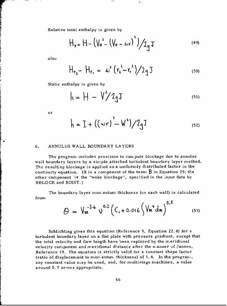
Relative total enthalpy is given by

Hr H- (v67- (V. - (49)2q

also

H Y27 r ~ (50)

Static enthalpy is given by

H,/ (51)

or

*= + ((, -I- w 2)/•J ,(52)

6. ANNULUS WALL BOUNDARY LAYERS

The program includes provision to compute blockage due to annulus

wall boundary layers by a simple attached turbulent boundary layer method.

The resulting blockage is applied as a uniformly distributed factor in the

continuity equation. (It is a component of the term B in Equation 25; the

other component is the "wake blockage", specified in the .nput data by

BBLOCK and BDIST.)

The boundary layer monmentum thickness (on each wall) is calculatedfrom v °

e9 = ,-4 (,+1o.o-16 Vcd) (53)

Schlichting gives this equation (Reference 9, Equation 22. 8) for a

turbulent boundary layer on a flat plate with pressure gradient, except that

the total velocity and flow length have been replaced by the meridional

velocity component and meridional distance after the manner of Jansen,

Reference 10. The equation is strictly valid for a constant shape factor

(ratio of displacement to monentun, thickness) of 1.4. In the program,

any constant value may be used, and, for multistage machines, a value

around 0. 7 seems appropriate.

66

The constant is determined from the specified blockage atthe inlet station which is assumed to occur as boundary layers of equalthickness on each wall. Then the integral is niade from the inlet stationto each station in the flow. If a hub does not exist in the machine at the

inlet, all the inlet blockage is assigned to the casing. Integration on thehub then commences at the "bullet nose" where the boundary layer isassuied to have zero thickness.

7. LOSS COEFFICIENT RE-ESTIMATION

The loss coefficient re-estimation procedure, if enacted, consistsof determining a diffusion loss coefficient and a shock loss coefficient, if

applicable, and summing these to give the total loss coefficient. This isdone for each streamline.

The diffusion loss coefficient is found by first calculating the diffusionfactor fron, Equation 2. The corresponding loss parameter is then inter-polated from each of the three loss parameter/diffusion factor curvesspecified to be used for the blade by I NEVAL I. These three curves giveloss parameters for 10, 50, a..d 90 per cent of the radial blade height(measured at the blade trailing edge), and the value for the particularstreamline radius is interpolhted fron, the three values. Then, the diffusionloss coefficient is given by

k) L3ra- Z~secj (54)

The shock loss coefficient, if calculated (NDEL 1 0), is found froman average Mach number at the presumed strong shock location. A suction-surface Mach number is found by expanding (or conmpressing) the relative

inlet Mach number through an expansion angle using the Prandtl-Meyerfunction.

The expansion angle is the sum of the value specified in the input(DELTA) and the incidence angle. If the blade geometry is not given at theblade leading edgc (NDATA =0), Lhe incidence is assumed to be zero. If therelative inlet Mach is less than unity, the expansion is calculated for aninlet value of unity. The shock Mach number is then taken as the meanof the relative inlet Mach number (or unity) and the suction surface Mach

67

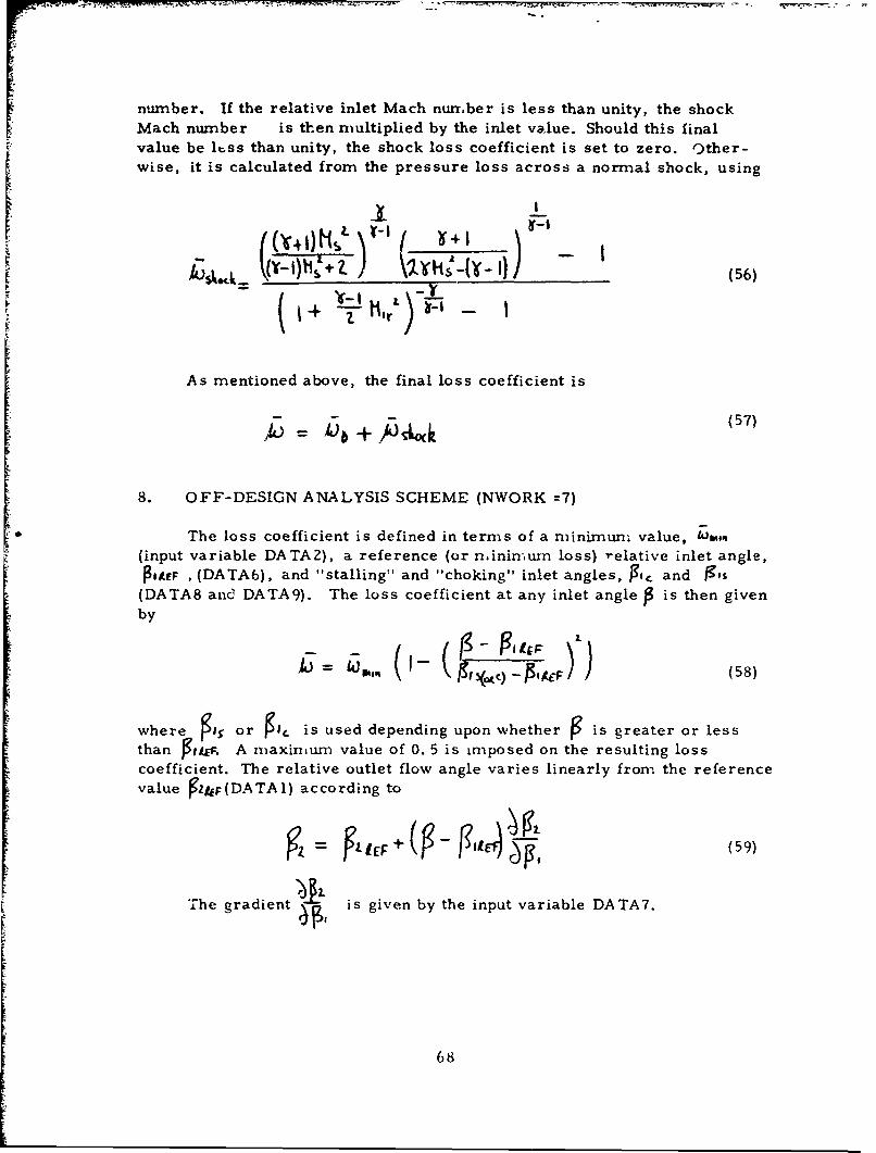
number. If the relative inlet Mach number is less than unity, the shockMach number is then multiplied by the inlet value. Should this finalvalue be lkss than unity, the shock loss coefficient is set to zero. other-wise, it is calculated from the pressure loss across a normal shock, using

+ +

- (t,. -4 )__ __ _ __ ___Z_ __ _I)__ _ (56)

As mentioned above, the final loss coefficient is

= (57)

8. OFF-DESIGN ANALYSIS SCHEME (NWORK =7)

The loss coefficient is defined in terms of a minimum value, Wiu,,n(input variable DATA2), a reference (or minimumn loss) relative inlet angle,

Poite , (DATAb), and "stalling" and "choking" inlet angles, gir- and Igo&(DATA8 and DATA9). The loss coefficient at any inlet angle P is then givenby

where r,$ or rc is used depending upon whether is greater or lessthan PI-. A maximunm value of 0. 5 is imrposed on the resulting losscoefficient. The relative outlet flow angle varies linearly from the referencevalue PgEF(DATAl) according to

+ P4 (59)

The gradient is given by the input variable DATA7.

68

9. BLADE GEOMETRY

For the purpose of determining relative flow ar~gles, deviation angles,and incidence angles, blade angles are required to be known on the strear-surface plane.

When the input variable NWORK equals 6, or blade leading edgegeometry is given, NWORK = 0 and NDATA >0, the angle given in the input(as DATA 1) is measured on the cylindrical plane. The corresponding valueon the streamsurface is found from

F'~~ubJ4 91 -(L (I1~J '' 9~)OS~u (60)

This equation is given in Reference 11. The aagle • is related tothe input blade lean angle by

+Ooa,4 = fx ty(61)

10. INTEGRATED PERFORMANCE

Machine performance is shown in the output in terms of pressureratio and isentropic efficiency on each streamline, and also as "integrated"figures for the whole flow.

In order to determine the integrated values, the following definitionsare made. At any station, the mean total enthalpy is given by

ýE = w/ (62)

The corresponding mean total pressure is given by

- . .6 (63)

69

From such values for the inlet station, a mean inlet entropy ( S,is found. An isentropic outlet totalenthalpy ( "I) is then fount" as a function

of the outlet mean total pressure ( I? ) and S, The integrated isentropicefficiency is then given by

S ii- • (64)

The inlet and outlet mean total pressures may also be used todetermine an integrated total pressure ratio.

11. RADIAL TRANSFER OF BLADE WAKES

A phenomenon of the flow through typical compre-cer rotor bladerows is the high losses recorded for blade sections near the tip. This isillustrated in Figure 2. 3 of Reference 6 where, for a given diffusion factor,rotor tip sections are shown to have a loss parameter fron, two to fourtimes larger than other blade sections. In compressor design and analysisprocedures, the traditional method has been to use different !;•s p,.rameter/diffusion factor curves for different blade section locations. The analysisin this subsection is an attempt to account analytically for the phenomenon.It is postulated that the result seen comes about not from differences in theboundary layer development mechanism, but from radial transfers of bladeboundary layer and wake flows, that is, secondary flows. These are causedby an imbalance of the radial forces on the slow-moving fluid particles, andthe inmbalance is the prinmary target of the following analysis. Because theresultant radial transfers are generally nmuch greater for rotors than stators,the effect is usually only easily discernable there, but the analysis may beapplied uniformly to rotors and stators. If the radial transfers are properlyaccounted for, the same wake generation model (loss coefficient correlation)may be used for all blade sections, provided it can be assumed that boundarylayer development on any blade section is affected at most to a second orderonly by the radial transfers.

The approach followed is to determine the ratio of radial shear stressto axial shear stress on an element of the blade surface boundary layers.It is then postulated that the extent of the radial movenment of the boundarylayer/wake material is proportional to the force ratio. The radial force isfound by considering the static pressure and centrifugal forces acting upona small volume of blade surface boundary layer. This is then related to theshear stress at the blade surface by the boundary layer thickness. Whenthe stress ratio is formed, the boundary layer thickness disappears fronmthe final result.

70

The radial stress is found from consideration of the forces actingon a small volume of the boundary layer, which show the net radial forceto be

Fr r - (65)

The small volume is in contact with the blade surface and, therefore,acts at the surface to produce a shear stress. If the boundary layer thick-ness is taken to be the conventional displacement t)ickness, then the shearstress is given by

+LLi. =(66)

The axial stress is found as follows. For a turbulent boundary layerwithout pressure gradient, Schlichting (Reference 9, Equation 21. 9) givesthe momentum thickness as

0 = o3�gX �J (67)

° and the shear stress is

(68)

At the blade trailing edge then, the axial stress is

S) 1(69)

The ratio of the stresses is

t' so S' C.7

71

If the shape factor is constant, we can write

000

It is now assumed that the tangent of the angle of the boundary layer/wakemovement is proportional to F1 . Thus a suitable axial dimension willyield the dimensional radial movement. For this dimension, the bladechord is taken. Hei e:

F r (72)

For our purposes, the free strean, velocity is the relative flow velocity.The constant K remains to be determined from experimental data. Inconjunction with the method of utilizing F" that is described below, a valueof 2. 0 appears to be approximately correct.

Equation 72 gives a radial movement distance at any radius, butsome further assumptions are required before this gives a loss profilemodified for the effects of radial transfers. Relative total pressure losscoefficient is approximately directly proportional to the thickness of thewake leaving the blade, and therefore the radial movement F is directlyapplied to a two-dimer'.ional loss coefficient distribution to produce thecorresponding three-dimensional distribution. Inputs to the numericalprocedure are loss coefficients presumed to be based upon blade elementcharacteristics (and therefore designated two-dimensional) for each strea.,-line, and F-values computed for each streaniline. These two quantitiesare spline-fit interpolated at 150 points uniformly distributed between huband casing. Each pair of values is taken to apply to an interval that liesabout the corresponding radial location. Thus at radius 1(ý , there is a losscoefficient /G and a shift F4 that apply to interval of width b where

In the case where ,I I or 150, 6) will be half the size of the other intervals.The loss coefficient fron. interval bt is redistributed according to F . itis assumed that the new distribution is a uniform division of th.* loss over

tda ( bt.3 ] ), so that in that region the new loss coefficient

attributable to OLO is

72

I ~+ FI) (4

The distributed loss coefficient "is seen at all of the 150 radii that themovement F crosses, including the starting point rj . In the event thatthe movement F3 prescribes a shift outside of the compressor annulus, F1is reduced so that the movement just reaches the annulus wall. Then 1431is proportionally larger than it would otherwise have been. This gives a"piling up" effect near a wall towards which there is boundary layer move-ment. The total loss coefficient at any radius is given by summing all of thei;3b components that apply to that radius. The last step is to determine losscoefficients for each of the streamlines that are being used in the basicflowfield calculation, and for which the original two-dimensional losscoefficients were given. To accomplish this, an eighth-order polynomialleast-squares fit of the 150rvalues is made, and then loss coefficientsat the desired radii are taken from the polynomial representation. Theleast-squares fit was introduced into the procedure because the 150-pointcurve exhibits some scatter and so cannot be used directly as input to acollating-curve interpolation scheme.

The procedure described above gives results that are, for engineeringpurposes, independent of the number of streamlines used to describe theflowfield. The selection of the number of points (150) at which the three-dimensional loss :oefficients are derived, and the use of an eighth-orderpolynornial fit for the three dimensional loss coefficient distribution do haveson.e effect on the results. As the number of points used to derive the losscoefficient distribution is reduced, the scatter of the resulting curveincreases, and effectively less radial transfer occurs. This is becausefewer of the shifts will be large enough to enter an adjacent accounting area.For larger numbers of points this effect diminishes, and there is generallylittle differeiice between the results for 100, 150, and 200 points. Aneighth-order polynomial fit normally retains all the essential features ofthe 150-point distribution, without being unduly influenced by the scatter.

12. TURBULENT MIXING OF THE AXISYMMETRIC FLOW

Assumptions that aro usuallymnade in turbomachine flowfield analystsare that the flow is inviscid and nonconducting, so that there is no transferof mass or energy across streamlines of the flow. The momentum equations

der'ved earlier (in Section V. 1) incorporate these assumptions as well asthe assumption that the flow i: axisyninietric. In reality, the flow isviscous and turbulent in n°.ture,and the effects of this are incorporatedinto the computation scheme.

73

The momentum equations are obtained by making the well-known

assumption that the flow may be described by the Navier-Stokes equations

for laminar flow, with the molecular kinematic viscosity replaced by anappropriate eddy viscosity. (See, for example, Reference 9.) For the

purpose of analyzing the turbulence, the flow is assumed to be containedby frictionless walls. Thus the result will be the effects of mixing of theflow without regard for annulus wall boundary layers. In fact, the entireflow is assumed to be of a boundary layer nature. Thus the momentum

equations, for axisymmetric, steady flow, and incorporating the boundarylayer type flow assumptionwhich eliminates second derivatives of velocityin the streamwise direction, are as follows:

V =) (76)

dWt (77)

It is now found convenient to consider the flow to be contained by a cylin-drical annulus. By making this assumption, it follows that the radialvelocity component must everywhere be very small compared to the othertwo velocity components, so that Equations 75, 76, and 77 may be written:

(78)

f~kr

74

t

ci~ - 'k~ _(80)

It is interesting to note that Equation 78 is the Simple Radial Equilibrium

Equation of turboniachinery, whereas Equations 79 and 80 retain viscousterms. T1.,s justifies a feature of the overall nethod that is introduced

later: the assumption that even when turbulent mixing effects are incor-

porated into computation, the ir.m,iscid momentum equations derived in

Section V. I may be used to compute the velocity profiles at each computing

station.

The boundary condition of frictionless walls may be expressed as:

-(81)

In order to determine the effect of turoulence upon the total enthalpy,

an energy equation is required. This is obtained from the energy equation

for laminar flow, neglecting conduction in the streamwise direction. Eddy

viscosity is again substituted for molecular viscosity, and the turbulent

Prandtl number is taken to be unity. Then the energy equation (for acylindrical annulus) is:

-(82)

The adiabatic wall boundary condition may be expressed as

- 0 at the walls (83)

(This assmes that 0

Continuity is satisfied at each axial location by use of the relation:

75

Sf' (84)

Equations 78, 79, 80, 82, and 84 with the boundary conditions givenby Equations 81 and 83 describe the selected model of turbulent flow, andare used to determine changes in the distributions of entropy, total enthalpy,and angular momentumw. The numerical procedure that is used is describedin Section VI. 10. The ee'y viscosity is presumed to be constant throughoutthe flowfield. This may be partially justified by considering that in the

typical situation where an eddy viscosity model is used, (such as the mixingof a free jet, or the shear layer between two parallel flows), there is oftena step change in vel' city at the upstream boundary, whereas in the case

of interest here the gradients in velocity are norm-ally similar in magnitude

throughout the flow. Application of the constant eddy viscosity model to

cases wvith step changes in conditions at the upstream boundary cculd be

expected to yield somewhat inaccurate profiles of conditions downstream,

although the basic trends would be reproduced.

76

SECTION VI

NUMERICAL PROCEDURES FOR AERODYNAMIC ANALYSIS

1. INTEGRATION OF DESIGN MOMENTUM EQUATION

The design-case momentum equation (Equation 19, 20, 23, or 24,as appropriate) is integrated as a lincai, first order equation in Vin

by assuming that only Vm is unknown. Then the integrating factortechnique may be applied to give:

I= Vle4 (-A (4j-?~) (I (-A (f1t ffl,~) ~ (85)

where, in the case of Equation 19,

Vm (86)

and (87)

eFor Equation 20, A reniains unchanged, and the last two terms inare replaced by:.

For Equation 23, the following definitions apply:

I ~ - -I-

"-.( )J (88)

77

B 3. 2IQ- &11 ( -,)_h( (89)

Equation 85 fails if A = 0, but then the following relation applies

ýJ 41+ (90)

In the computer program, the switch from Equation 85 to Equation 90 ismade when IA I io'

Equation 85 (or Eqdation 90) is applied to the interval between eachadjacent pair of streamlines in turn. A single value of the paranmeters Aland B is determined for each interval. Gradients in the direction of thecomputing station are found using:

Gradients in the strean,line direction are found from, (for Station I),

FF Fr Fr F /27 (92)

78

At the first and last computing stations, and du-ing the first pass of

calculation, the streanlwise gradients are asswuned to be zero. A value is

determined from Equation 92 for each streamline, and then an average value

is used in each streanmtube. This procedure is followed for each quantiLythat is given on a streamline rather than for a streantube. The streamlineslope angle • is given, at Station I, by

,,Y* )/t(93)

At the first (last) conmputing station, is given by

i- (94)

The radius of curvature of the streamlines is assumied to be zero atthe first and last stations and elsewhere is deternined from.:XT (95)-- X+ I( ,.- ) - t0 +( -2,)- (95)

The m•ethod of solution described above is based upon the assumptionthat the paramaeters A and B art- fixed. In fact, they are dependent to a

varying degree upon the xi.eridional velocity, and so the determination ofthe meridional velocity is iterative. " meridional velocity profile isestimated, the paramieters A and B are determined, and a new velocityprofile is deterin.ined from, the mid-streamline velocity and the A and Bparameters. Son,m instability in this procedure was observed on occasion,and therefore a relaxation factor 1Z has been introduced into the procedure

for the new estim ate of the iz ceridional velocities, thus:

r4V j o + (VpioP#Ae - VVolJ) (96)

where

(97)

79

The nondimensional change in VN in Equation 97 is computed as an - -

coordinate weighted average, and R is not permitted to be less than 0. 1.

So-ie lin.its are set on the values of Vn that mnay be recorded foreach streamline. A lower lhi.it of 1.0, and an upper limit of twice thevalue on the n.id-stream-line are imposed, if necessary. For the case ofSubroutine UD0308 only, there is also an upper limit equal to the localspeed of sound.

When a new meridional velocity profile has been estinmated by theabove procedure, the entropy distribution is recalculated if losses arespecified in such a way that the entropy is a function of meridional velocity.Then the continuity sunmmations described separately below are made and,

if continuity is not satisfied, or the resulting neridional velocity profilediffers fron; that initially assumed, a new iteration is started. Themaximum number of permnitted iterations is controllea by the variableITMAX, which is set (separately) to 20 in both Subroutine UD0308 andSubroutine UD0326.

2. INTEGRATION OF ANALYSIS MOMENTUM EQUATION

The analysis momentuii, equation (Equation 17, 18, 21, or 22, asappropriate) is nonlinear in Vm , and therefore a different schen.e to thatdescribed above for the design case equation is used. All the gradients andstreamline characteristics are computed as for the design case. Using anestimnate of the average meridional velocity in a given streamtube, thegradient dAm"/d.o is conmputed from, either Equation 17, 18, 21, or 22.This gradient is then used to step to the next streaiiline using:

I

The velocity determined by Equation 98 is not permicted to be less ihan 1.0nor greater than thiee tin.es the nmid-streamline value. Because the gradientdepends upon the mieridional velocity, tne velocity cietermination by dhisn.eans is iterative, and up to 10 loops are allowed.

When a new meridional velocity profile has ocen established by theabove procedure, the entropy distribution is recalculated if losses arespecified in such a way that the entropy is a function of meridional velocity.Then the continuity suwmmations described sepa':ately below are made and,if continuity is not satisfied, or the resulting n.eridional velocity profile

80

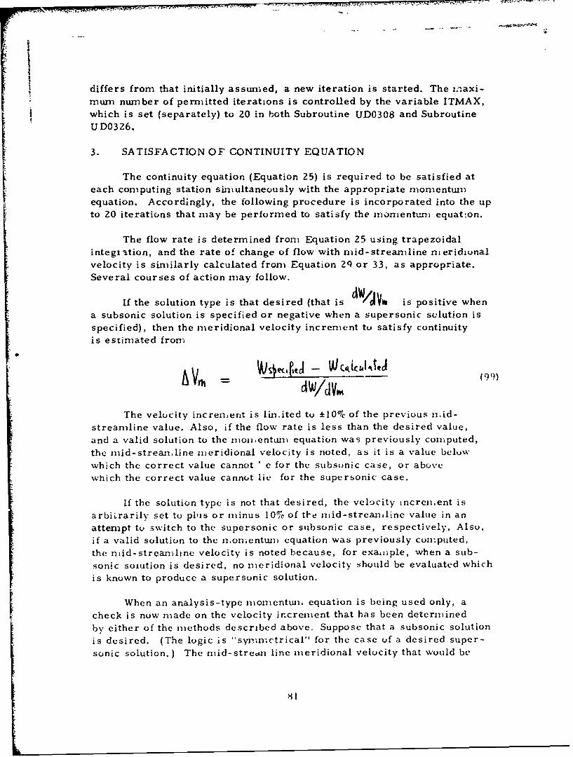
differs from that initially assumed, a new iteration is started. The inaxi-

mum number of permitted iterations is controlled by the variable ITMAX,which is set (separately) to 20 in both Subroutine UD0308 and Subroutine

UD0326.

3. SATISFACTION OF CONTINUITY EQUATION

The continuity equation (Equation 25) is required to be satisfied ateach computing station simultaneously with the appropriate momentum

equation. Accordingly, the following procedure is incorporated into the upto 20 iterations that may be performed to satisfy the momentum equatton.

The flow rate is determined from Equation 25 using trapezoidal

integiation, and the rate of change of flow with mid-streamline nieridionalvelocity is similarly calculated from Equation 2q or 33, as appropriate.

Several courses of action may follow.

If the solution type is that desired (that is A / W is positive whena subsonic solution is specified or negative when a supersonic solution isspecified), then the meridional velocity increment to satisfy continuityis estimated from

AVit (99)- a /d VM

The velocity increment is lin.ited to +I0% of the previous mid-streamline value. Also, if the flow rate is less than the desired value,

and a valid solution to the monentuim equation was previously comnputed,

the mid-streamline meridional velocity is noted, as it is a value belvw

which the correct value cannot ' e for the subsonic case, or above

which the correct value cannot lie for the supersonic case.

If the solution type is not that desired, the velocity incren.ent is

arbitrarily set to plus or minus 10% of the miid-streamline value in anattempt to switch to the supersonic or subsonic case, respectively. Also,

if a valid solution to the n.onmentwi- equation was previously com.puted,the mid-streamline velocity is noted because, for exatnple, when a sub-sonic soiution is desired, no meridional velocity should be evaluated which

is known to produce a supersonic solution.

When an analysis-type momentun, equation is being used only, a

check is now made on the velocity ir.cr•ment that has been determined

by either of the methods described above. Suppose that a subsonic solution

is desired. (The logic is "symn,.etrical" for the case of a desired super-

"sonic solution.) The mid-streai line meridional velocity that would be

81

given by modifying the previous value by the calculated increment ischecked to see if it would be higher than the lowest value which has beenshown to imply a supersonic solution, Vwh sv•ir . If so, a new incrementis calculated. The new increment is given by

--- (100)

Thus, the new velocity will be within the range of possible values,and will generally refine the previously established lin.its for the range.

A similar check is made with respect to the mininimun plausiblevelocity, that is V0 1 , the highest velocity shown to inmply a subsonicsolution at a flow rate lower than desired.

The meridional velocities on each streamline are incremented bythe amnount derived as described above, and a lower limit of 1.0 is imposedon the value produced.

If Subroutine UD0308 is being used (input variable NEQN = 0 or 1),an upper linmit equal to the local sound speed is also imposed upon thenieridion:,l velocity at each streanline. In this case, the maximum n1id-

sirean.line nieridional velocity allowable for a supersonic solution( Vj Sjýe, ) is set equal to (the sound speed x 1.05) initially.

When Subroutine UD0326 is being used (input variable NEQN - 2 or 3)VO to•v" is initialized to 2500.0. In both cases, the nininiwll

permitted velocitv for a subsonic solution is initialized tz zero.

A check is made on the convergence of the inomentwii and continuityequat,ons, and,if these do nut both cunveree. a new iteration is started,'ubject to the naximumi muiber of iterations permitted by the variableITMAX. If a new iteration is started, the entropy distribution is recalcu-lated if it is a function of meridior.al velocity, and then the nmomentulnequation integration plocedure is entered as described above.

4. STREAMLINE RELOCATION ITERATION

The positions of the strean.line are determined iteratively using thecondition that a constant fraction of the total flow should lie in each stream-

tube. The flow distribution used to revise tht.e strean.line cooccinate is afunction of the streamnline characteristics, and, therefore, the calculationis potentially unstable. :N relaxation factor is derived in the followinganaly-,is, which is based upon a similar analy.,is performed by Wilkinsonfor two-dimensional flou%, Refezence 12.

8 2

Consider a swirling flow in a cylindrical annulus, with no enthalpyor entropy gradients. Computing stations are uniformly spaced Ax apart,and are radial. Equation 20 may be applied, and simplified to give

, _ h, v2 00 c,) )1)

By asswuming orly small deviations from midradiu,. conditions, wecan approximate Equation 101 by

= -r. k (102)T r.

If we introduce an error in the streamiiline radius at one station only.then the corresponding radius of curvature is

S-- (103)

Combining Equations 102 and 103 gives

Al = yo K (104)

or

= -(~[XZ (105)

Mass flux distribution is proportional to V , and again, we approx-imate the distribution, using I

3 (106,

83

and

)4k 1 107)

For a high radius ratio, the flow between radii r, and Y~ is propor-

r

tional to and from the previous equations

(, Vw.<r = ,,,l,_.+ •• ,•

(108

To deternmine the effect of the error, we compare the predicted

location of the screamline that divides the flow into two equal parts with its

correction location, that is when = 0 The predicted location, YX , may

be found frou., the following equation

4"/ (109)

Using Equation 108, and assuming

Y'u -Vi4 XL (110)

this yields

where

84

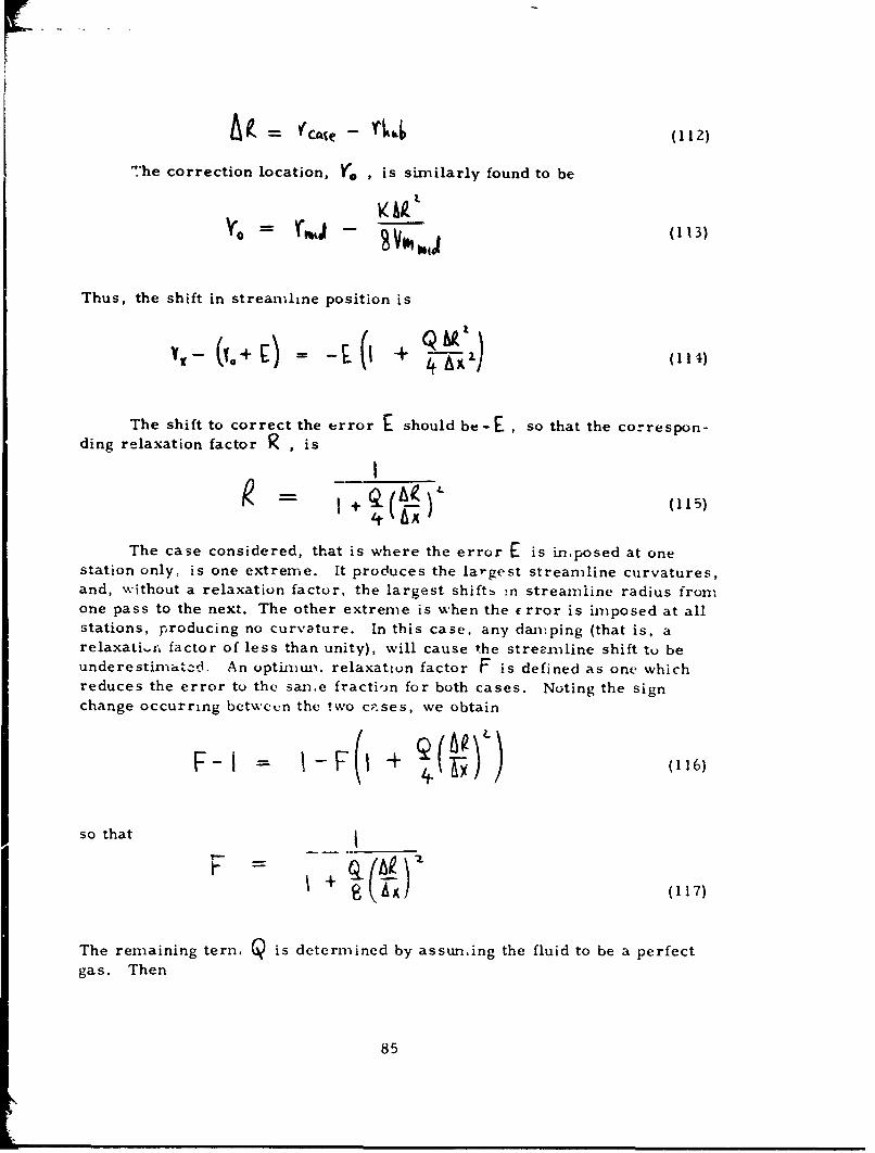
"'he correction location, ro , is similarly found to be

V"0 S - 1 (113)

Thus, the shift in streamline position is

+- ( + (114)

The shift to correct the trror E should be-E , so that the correspon-

ding relaxation factor J , is

x-L

The case considered, that is where the error E is inmposed at onestation only, is one extreme. It produces the largest streamline curvatures,and, without a relaxation factor, the largest shiftb ,n streamline radius fromone pass to the next. The other extreme is when the f rror is imposed at allstations, producing no curvature. In this case. any dam ping (that is, arelaxati..a, factor of less than unity), will cause the streanmline shift to beunderestimatcd. An optinnuri. relaxation factor F is defined as one whichreduces the error to the same fracti-'n for both cases. Noting the signchange occurring between the two ca.ses, we obtain

F-.I I (116)

so that

S+ • (117)

The remaining tern, Q is determined by assuming the fluid to be a perfectgas. Then

85

/VM +r ( (118)

and

Q= = i-K(119)

For the case when the relative flow angle is specified, the analysis startsfrom Equation 18, and, following the same steps as fur the case above,the final result is

I

F' = C (120)

and

void (121)

In the program, the length AR is taken as the computing stationlength and the length &X is taken as the meridional distance at mid-annulusto the nearer of the two adjacent computing stations. The constant S inEquations 117 and 120 has been found fron experience to often need reducingto 6 to ensure stability. It is input as the variable RCONST. The Machnumber squared that appears in Equations 119 and 121 is linmited in theprogram to the value input as XMMAX, and 0. 6 has been found to begenerally satisfactory. The relaxation factor finally determined is appliedto the streamline coordinate I. , thus

- ~ ' i~ ~ I J + F J c ((1 2 2 )

5. CONVERGENCE CRITERIA

The preceding four subsections have all described iterative proceduresinvolved in the overall determination of a solution. The convergence of each

86

t , of these procedures is nmeasured by nmeans of a tolerance., applied asS~described below, and related to a single input variable, TOLNCE. The

normal value for this is 0. 001.

When the meridional velocity at a station is determined by inte -

gration of the analysis form of thc nmonenttw• equation, the velocity at any

streaiL~line is iterati ely determlined in a stepping procedure froii, the

adjacent streanmline that is nearer to the mid-streamline. This iteration is

considered converged if the. calculated velot ity repeats to within a tolerance

of TCLNCE/5. 0, applied nondilnensionally. Thus. :f TOLNCE :0.001. two

successive m~eridional velocities ii~ust be w'ithin one part in 5000.

Following adjustnment of the velocity level on all streaii lines,, a ch•.ckis madL to see if both continuity and mom~entugn are satis~ied. The toler-

ance used is TOLNCE/5. 0. unless ? loss coefficient re-estizi.attton is

specified at the station (NE VAL > 0), when the tolerance is TOLNCE/10. 0.

Trhe continuity check is that the calculated flow niust equal the specifiedvalue to within the stated tolerance, applied nondin~ensionally. Then the

ii omentua•, equation solution is checked by requiring that the vclocities

equal those estimlated to within the samxe tolerance, applied nondiii.ensionally.

If loss coefficient re-estim~ation is specified at a com•puting station,

an extra iteration for the loss coefficients is involv'ed. Convergence of this

iteration is m~easured by comparing the estiziated ii.eridional velocities with

those calculated, and the tolerance applied is TO)LNCEi 5. 0. With LITER

set to say 5, this iteration will probably not converge to within the above

st•.ted tolerance during~ the first few pas.,es through the program•.

Overall convergence of the solution is determ~ined by two checks that

are miade at the end of each pass. The nmeridional velocities at each mesh

point nr,ust repeat to within a tolerance of TOLNCE. applied nondizl.ensionally.

Also, the proportion of •.ile total flow that p;asses between the hub and each

streamlhne unit be \tith .n TCLNCE of the desired value at every computing

station. For examlple, if somle streamline should have 0. 5 of the flow

betwveen it and the hub, and TOLNCE =0.00~i, the acceptable range is froml•

0. 499 to 0. 501.

:6. PRANDTL-MEYER FUNCTION

The Prandtl-Meyer fun.~tion is given by Equation 55, and in the course

of re-estimating the loss coefficients, it this is specified to be done,it isdesired to determine the Mach num~ber corresponding to a given an le,_ "9-

This is done iteratively using Newton's method, with the quantit -i*l

being so rather than M ). An initial estim~ate, F6 , of |•l-is nade

equal to~I-Mm 40.! where He is the Mach number before the expansion.

2 (123

This is repeated until and Fi. are within 0. 000001 (subject to a maximiunutmber of iterations of 20).

7. STAGNATION POINT PROVISION

If the "hub" radius at the inlet station is zero, a stagnation point isincorporated into the solution at the last station for which the "hub" radiusis zero. This must occur upstream• of any blade rows, and the whirl

velocity at zero radius nust be zero. The stagnation point is handled byimposing the zero meridional velocity at that point, and only integratingthe momentum equation inwards as far as the second streamline. The con-tinuity sunimation includes the innermost strean.line in the nornial t1.anner.A finite curvature will be shown in the results at the stagnation point, butthis is of no consequence because the momentunm equation is not computedin the innermost streanitube.

8. INTERPOLATION

The various tabulatea data input to the progranm is interpolated at thestreamline by the method specified by the input variable NTERP. Twoalternatives are available. If NTERP = 1, linear point-to-point interpolation(or extrapolation) is performed. This is not to be preferred generally,assuming the data points define a smooth curve.

If NTERP = 0, spline-fit interpolation is performed. The splinecurve consists of a series of algebraic cubics, one equation applying betweeneach adjacent pair of data-points. The coefficients are determined Such thatthe resultant curve passes through each point, and has continuous first andsecond derivatives. Various boundary conditions nmay be in,posed at eachend of the curve; in this case the second derivative at the end point is setto zero.

9. DEVIATION ANGLE DETERMINATION FORANALYTIC MEANLINE BLADE SECTION

The determination of the deviation angles for analytic n-eanline bladesis performed in Subroutine UD0319. A description of the procedure used isincluded in this section. The subroutine is only entered if the inputvariable NAERO = 1.

88

S.. . ............

The trailing edge leviation is calculated from

Solo 4 k .~t~ . (e ~))+ 5 b (124)

The parameters 5s lQ/•c , and $4) are given in the input as variablesXKSHPE, AC, and DELTAD, respectively. The camber (9) and solidityi ( O ) are derived from the basic determination of the blade sections. Theremaining parameters, , and .o , are found by inter-

polation from data given in Figures 161, 172, 164, and 195 of Reference6, respectively. Equation 124 is based upon Equations 269 and 271 ofReference 6, except that,when a parameter is shown in Reference 6 to bea function of relative air inlet angle, blade inlet angle is substituted inthis orogram.

For locations, that is,computing stations, within a blade row, thedeviation is determined fromn-

* 0 crekf3Tei(125)f~fe

The fraction is interpolated from the input variables DVFRAC andDM as a function of the location on the meridional chordline and, ifNRAD > 1, as a function of stream surface radius at the trailing edge.

The "station control card", blade speed, blade geometry, loss values(interpolated at the appropriate radii), and deviation angles are output ontothe file specified by unit LOG5 for each computing station within the blade,or at the blade trailing edge, in the format required by the aerodynamicsection. The station control card has NDATA set equal to the number ofstreamsurfaces on which blade sections are produced, 14WORK = 6, andNDIMEN = 0. The remaining variables are set according to the values inthe input data for that station.

At the blade leading edge, no deviation calculation is required, but a"station control card", a speed of zero, and blade geometry are output ontothe file specified by unit LOG5 if the input variable IFANGS for the leadingedge station is 1. The station control card has NDATA set equal to thenumber of streamsurfaces on which blade sections are produced, and allremaining variables on the control card are set to zero, except NOUTI,NOUT2, and NOUT3,which are reproduced as read in.

89

L

10. TURBULENT MIXING CALCULATION PROCEDURE

The equations derived in Section V. 12 describe the changes in thedistribution of conditions along "streamlines" of an axisymmetric, turbulentflow in a cylindrical annulus. In Section V. 1, equations we'-e derived forthe stationwise variation in meridional velocity of an axisynimetric, inviscidflow in an arbitrary annulus. These show the meridional velocity gradientto be a function of the distributions of entropy, total enthalpy, and angularmomentum (as well as the streamline characteristics). In order to incor-porate the rr.ixing calculations into the overall computations, first theturbulent flow equations are used to determine modifications to the station-wise distributions of entropy, total enthalpy, and angular momentum.

Then, th": r.-dified distributions are used in an inviscid momentum equa-tion to compute the meridional velocity profile. This method is ised for theinterval between each successive pair of computing stations from the firstto the last, for each pass through the iterative procedure to determinethe streamline locations, and hence the final solution. On a step-by-step

basis, the computation proceeds thus:

1) At Station 1, an inviscid momentum equation gives the meridionalvelocity distribution.

2) The turbulent flow equations are applied for the interval Station1 to Station 2 to give the distributions of entropy, total enthalpy,and angular momentum at Station 2.

3) If a blade-row lies between Stations 1 and 2, the distributionsof entropy, total enthalpy, and angular momentum at Station 2are redetermined, using the mt, Gified distributions determined

in step 2 as the inlet conditions. Thus the effects of the blade-row (if one exists) are superimposed upon the mixing calculation.

4) An inviscid momentum equation is used to determine themeridional velocity distribution at Station 2.

5) Steps 2, 3, and 4 are repeated for the intervals Station 3 to 4,4 to 5, and so on, to the last computing station.

6) A new streamline pattern estimate now exists, based upon the

meridional velocity profiles computed for each station. Unlessthe overall solution is converged, control returns to Step I foranother pass.

The application of the turbulent flow equations, Step 2 above, is made

as follows. The interval cf con,pressor annulus is approximated by a

cylindrical annulus, for which the hub and tip radii are the mnean hub and

90

tip radii of the segment of the compressor az..-alus, and for which thelength- is the nmean length of the segment of compressor annulus. Theevolution of conditions at the downstream boundary from those at theupstrean, boundary is made by stepping downstream through a number ofequal increments. The method by means of %hich the number ofincrements is chosen is described below. Each increment may be con-sidered to have an upstream boundary and a downstream boundary.Conditions at the first upstream boundary are those at the upstreamboundary of the whole mixing interval. Conditions at the downstreamboundary of an intermediate step become the upstrean, boundary conditionsfor the next step, until finally for the last step, the downstream boundaryconditions are those sought for the downstream boundary of the mixinginterval. Inputs to the calculation are, at the upstrea.i boundary, the nrrid-streamline static pressure, the mid-streamnline n.eridional velocity (bothas computed previously by the inviscid equations), the radial distributionsof entropy, total enthalpy, and angular momentum, and the eddy viscosity.For each mixing step, the calculation is made as follows:

1) The radial component equation (Equation 78) is integratedto give the static pressure distribution at the upstreamboundary. Equation 78 is written in the following form:

V Ar (126)

This equation is used to step from streamline to streamline,mean values of the quantities involved being used in eachradial interval. As the density distribution is not known,this must be determined itervatively from the static pressuresand the entropy.

2) For each streamline, the static pressure and entropy give thestatic enthalpy. The total and static enthalpies give the totalvelocity. The total velocity and tangential velocity componentgive the axial velocity component.

3) For the first step only, a continuity summation is made todetermine the flow rate.

41 The energy equation (Equation 82) is appliec )n each streamlineto give the total enthalpy distribution at the downstrean-. boundary.Equation 82 is written as follows:

91

WH - (127)

The method of obtaining all radial derivatives is describedbelow.

5) The tangential component equation (Equation 79) is used oneach streamline to give the downstream tangential velocitycomponent distribution. Equation 79 is writter.:

AV, Y r128)

6) The mid-streamline, downstream static pressure is estimated(as being equal to the upstream value).

7) The downstream radial distribution of static pressure isdetermined as was the upstream distribution in Step 1.

8) The axial component equation (Equation 80) is applied on eachstreamline for the downstream axial velocity distribution.Equation 80 is written:

I AVL - (129)

9) For each streamline, total enthalpy, tangential and axialvelocities yield static enthalpy. Static enthalpy and staticpressure give density. A summation is made for the flowrate at the downstream boundary.

10) If the flow rate computed in Step 9 differs from that establishedin Step 3, the mid-streamline static pressure is re-estimated,and control returns to Step 7. (The method of re-estimatingthe static pressure is given below.) Otherwise, controlpasses to Step 11.

92

11) Entropy at the downstream boundary is given by staticenthalpy and static pressure. Downstream boundary conditionsbecome upstream boundary conditions for the next step, andcontrol returns to Step I.

Radial derivatives of the form yO occur in Equations 127,

128, and 129. For streamlines away from the walls, the following methodis used:

SJ _ a _ .,(130)

Values near a wall must reflect the boundary condition: at

the wall. If the streamlines are numbered 1, 2, 3, ... starting at the wall,then

+ (131)

A value for streamline 1 is obtained by linearly extrapolating thevalues for streamline 3 and 2 to the radius at the wall. The vaiue at streamline3 is given by the general formula, Equation 130.

The number of steps into which each interval must be divided iscontrolled by the stability of the three equations used to step in the axialdirection. Consider the energy equation, and a linear variation of enthalpywith radius. The effect of mixing will be to reduce the enthalpy gradient,

but not to reverse the sign thereof. If an excessively large axial step ismade, the sign of tme gradient will change, and so the limit for stabilityis when the gradient is just eliminated. Writing the energy equation inapproximate form:

(132)

93

The critical streamlines are those adjacent to the walls. If the streami

lines are numbered 1, 2, 3. ..... starting at the wall, and equispaced, then,from Equations 130 and 131 (and for a linear enthalpy distribution):

a.01 41tt - (. U L133)Stitoowdiv 2 V r

QJR&IJ11ffiCK(134)StA4IKIVL Ar

where 6 is the change in enthalpy between stream.lines and Ir isthe streamline spacing.

The limit for stability is when:

or

and from Equations 133 and 134

61 > (135)

The san.e analysis niay be applied to the tangential and axial componentequations, with the same result. In practice, the limit of A- has beenfound to be slightly nmore than half the value given by Equation 135. Theprogram selects the number of steps to be four times that given býEquation 135, but even this will often lead to only one step being requiredfor each mixing interval.

94

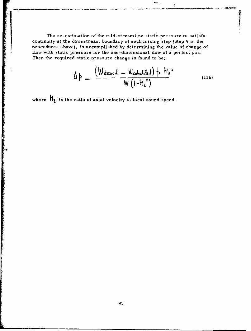
M!

The re-estimation of the n.id-streamline static pressure to satisfycontinuity at the downstream boundary of each mixing step (Step 9 in theprocedures above), is accomplished by determining the value of change offlow with static pressure for the one-dinmensional flow of a perfect gas.Then the required static pressure change is found to be:

(A 1 (136)

where H, is the ratio of axial velocity to local sound speed.

95

SECTION VII

PROGRAM OPERATION AND STRUCTURE

1. IMPLEMENTATION

The program is basically written in USA Standard FORTRAN andshould therefore be compatible with all current medium-to-large computingsystems, except as noted below. All development running has been done ona Control Data Corporation 6600 computer at Wright-Patterson Air ForceBase. The operating system was changed from Scope 3. 3 to Scope 3.4during the program development period. The operating systen, includesCALCOMP software and hardware for on-line precision plotting.

The program is loaded in three principal overlays by a small residentmain program, and the demands of the CDC Scope overlay scheme areincorporated into the coding. Under Scope 3. 4, the central memory require-ments for the three overlays are approximately as follows: the aerodynamicsection, 115K; the analytic meanline blade section, 125K; and the arbitrarymeanline blade section, 105K. These requirements would be reduced about10K under the more widely used Scope 3. 3 system. The aerodynamic sectionis divided into a principal loading and two alternative loadings. The alterna-tive loads are Subroutines UD0308 and UD0326, which handle two alternativemomentum equation formulations selected by the input variable NEON. Inorder to compile and run the program under systenms other than CDC Scope,the overlay-related calls will need to be modified. These are:

1) Card $MN$. 24 in Program UD0300 (the main program) whichcalls the analytic meanline section, cards $AN$. 2 and $AN$. 3.

2) Card $MN$. 27 in the main programwhich calls the aerodynamicsection, cards $AR$. 2 and $AR$. 3.

3) Card $MN$. 31 in the main program, which calls the arbitrarymeanline section, cards $AB$. 2 and $AB$. 3.

4) Card $AR$. 229 in Program UD03AR, which calls ProgramUD0308, cards $08$. 2 and $08$. 3.

5) Card $AR$. 231 in Program UD03AR, which calls ProgramUD0326, cards $26$. 2 and $26$. 3.

With the exception of the main program, each of the programs referred toabove is, in conventional FORTRAN terms, a Subroutine. The PROGRAM

96

statement attached to the main program, Card $MN$. 2, is peculiar to theCDC Scope system, and defines the following file usage by the program:

FORTRANCDC File Name Variable Name Value Description

"INPUT LOGI 1 Card readerOUTPUT LOG2 z Line printerPUNCH LOG3 3 Card punchFILE2 LOG5 5 Scratch fileFILE3 LOG6 6 Scratch filePLOT - CALCOMP plot file

- , The numerical values are assigned to the FORTRAN variables in the mainprogram starting with card $MN$. 8. (LOG4 is redundant.) LOGI andLOG2 are also defined in Subroutine UDGI on cards $GN$. 4 and $GN$. 5.

"Calls are incorp-rated into the coding to subroutines that are assunmedto be available as part of a CALCOMP plotting package. All the plotting isonly performed optionally so that the program may be used on a system that

i* does not include these routines in its library. However, it may be necessaryto add a dummy subroutine with the entry-point names PLOT, SYMBOL,NUMBER,AXIS, and LINE, as some systems will not permit programexecution with unsatisfied external references.

2. PROGRAM LOGIC

The complete program comprises of 42 FORTRAN programs andsubprograms. They are distributed among the three principal overlays asfollows:

a. Resident

Program UD0300. The main program, controls entry to eachsection.

b. Aerodynanic Section

Program UD03AR. The "main program" for the aerodynamicsection, controls logic within the section.

Subroutine UD0301. Spline-fit or linear interpolation and gradientdetermination.

Subroutine UD0302. Reads input data.

97

Subroutine UD0303. Checks lines printed per page.

Subroutine UD0304. Axisymmetric turbulent mixing calculations.

Subroutine UD0329. Determines rz;:al derivatives for mixingcalculation.

Subroutine UD0305. Handles interpolation of input data at a particularcomputing station.

Subroutine UD0306. Modification of loss coefficients to account forradial blade-wake transfers.

Subroutine UD0330. Solves simultaneous linear equations for least-square fit.

Subroutine UD0307. Determines entropy, rothalpy or enthalpy, andwhirl velocity at a computing station.

Subroutine UD0309. Re-estimates loss coefficients.

Subroutine UD0310. Annulus wall boundary layer calculation.

Subroutine UD03 11. Regular printed output.

Subroutine UD0312. Precision-plot output.

Subroutine UDGI. Reads data describing fluid.

Function UDG2. Enthalpy =f (entropy, pressure)

Function UDG3. Entropy = f (pressure, enthalpy)

Function UDG4. Pressure z f (enthalpy, entropy)

Function UDG5. Specific weight = f (enthalpy, entropy)

Function UDG6. Enthalpy = f (pressure. tenmperature)

Function UDG7. Temperature = f (enthalpy, entropy)

Function UDG8. Ratio of specific heats r f (enthalpy, entropy)

Function UDG9. Square of Mach nunber - f (static enthalpy,entropy, square of velocity)

98

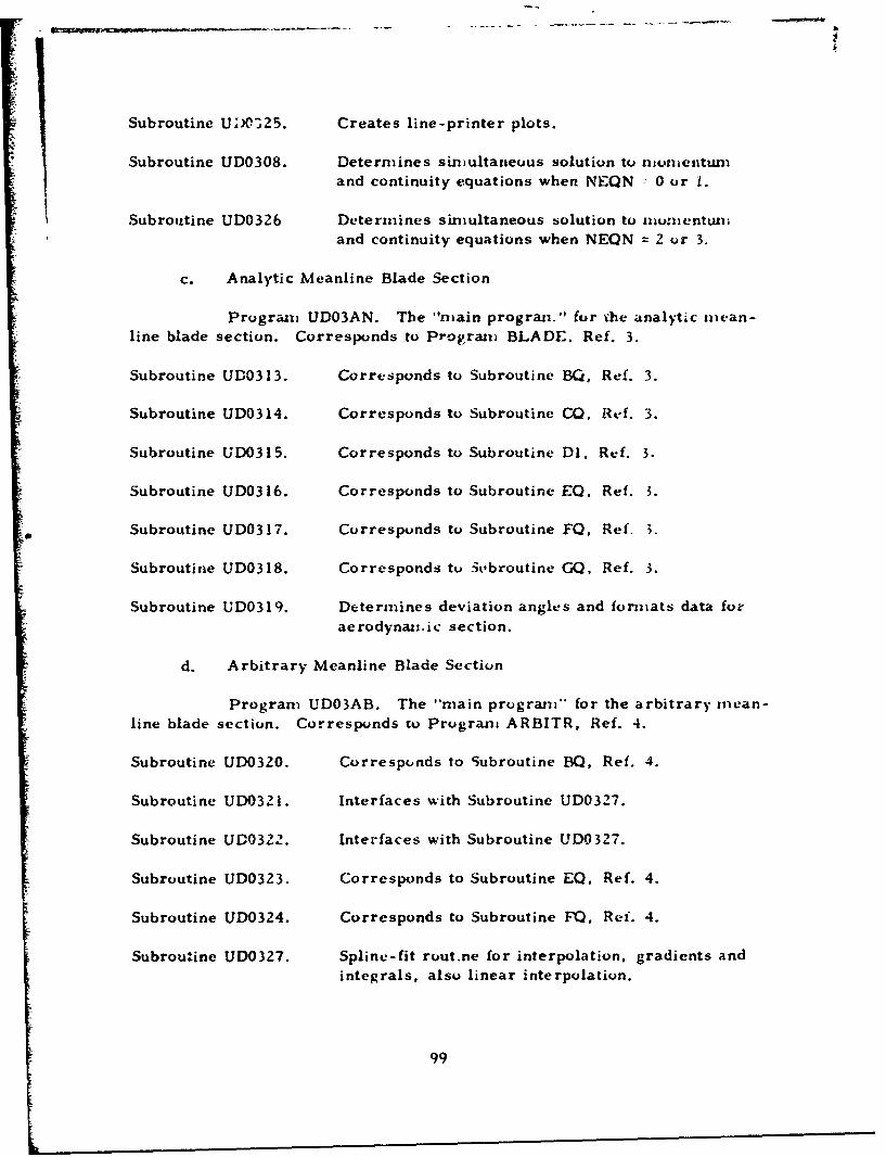
Subroutine U;.325. Creates line-printer plots.

Subroutine UD0308. Determines simultaneous solution to nmomnentumand continuity equations when NEQN 7 0 or 1.

Subroutine UD0326 Determines simultaneous solution to mouentwLaand continuity equations when NEQN = 2 or 3.

c. Analytic Meanline Blade Section

Program UD03AN. The "main progran." for ýhe analytic mean-line blade section. Corresponds to Program BLADE. Ref. 3.

Subroutine UD0313. Corresponds to Subroutine 80, Ref. 3.

Subroutine UD0314. Corresponds to Subroutine CO, Ref. 3.

Subroutine UD0315. Corresponds to Subroutine DI, Ref. 3.

Subroutine UD0316. Corresponds to Subroutine EQ. Ref. 3.

Subroutine UD0317. Corresponds to Subroutine FQ, Ref. 3.

Subroutine UD0318. Corresponds to itbroutine GQ, Ref. 3.

Subroutine UD0319. Determines deviation angles and formats data foraerodynamtic section.

d. Arbitrary Meanline Blade Section

Program UD03AB. The "main progran'" for the arbitrary mean-line blade section. Corresponds to Program ARBITR, Ref. 4.

Subroutine UD0320. Correspnds to Subroutine BQ, Ref. 4.

Subroutine UD0321. Interfaces with Subroutine UD0327.

Subroutine UD0322. Interfaces with Subroutine UD0327.

Subroutine UD0323. Corresponds to Subroutine EQ, Ref. 4.

Subroutine UD0324. Corresponds to Subroutine FQ, Ref. 4.

Subroutine UD0327. Spline-fit rout.ne for interpolation, gradients andintegrals, also linear interpolation.

99

The overall program logic is illustrated by the flow chart in

Figure 2. This shows all the significant actions in Program UD0300,expressed by n.eans of the FORTRAN variables and statement labels.

Start

If (NANAL. EQ. 0)I

DO 120 K= 1, NANAL120 CALL Analytic n.eanline section

130 V_If (NAERO. EQ.O

CALL Aerodynamic section

140

If (NARBIT. EQ. 0-

IDO 150 K= I, NARBIT

150 CALL Arbitrary n.eanline section

160

Stop

Figure 2. Overall Progranm Logic

Details of the operation of the analytic meanline section may

be found in References 3 and 5. The only significant modification made inincorporating the progranm described therein into Program UD0300 is theaddition of Subroutine UD0319. This subroutine is entered once as a final

operation if data from the analytic nmeanline blade section are required as

input for the aercdynamic section.

The arbitrary meanline blade section operates basically asdescribed in References 4 and 5, but a nev method of generating the mean-

line has been developed. Previously, a number of meanlines were

examined, based upon .k range of boundary conditions at the leading edge.The n.eanline was then selected from those obtained on the basis of theminimum number of inflection points and the largest minimum radius of

100

3

curvature on the meanline. The segment of meanline between each pointwhere the blade angle was specified (a computing station in the aerodynamicanalysis) was an algebraic cubic, so that the resulting meanline was a spline-

curve restrained to give the desired blade angle at each computing station.At the leading edge, the radius of curvature of the meanline was defined.The new procedure is to fiL a spline-curve through the specified angles ateach computing station. Then the analytic integral of the spline curve givesthe meanline which is therefore a piece-wise quartic. Boundary conditionsused for the spline-fit are that the second derivative be zero at each end.The new procedure has been found to give meanlines with generally largerminimum radii of curvature than the old procedure, and, in some instances,to give a satisfactory meanline when none could be found using the oldprocedure.

The logic of the aerodynamic section is illustrated by the flowchart shown in Figure 3, which is essentially a flow chart for ProgramUD03AR. All significant actions and calls to subroutines (other than toSubroutine UD0301 for interpolation) in the program are shown.

3. PROGRAM AND SUBPROGRAM DESCRIPTIONS

a. Program UD0300. Cards identified by $MN$. This is the mainprogram and controls entry to each section, as shown in Figure 2.

b. Program UD03AR. Cards identified by $AR$. This is the mainroutine of the aerodynamic section, and it controls the logic of the section,as shown in Figure 3. In terms of conventional FORTRAN it is a sub-routine, but is sl-own as a program because of the use of CDC Scope ovc y.Some significant points are distributed in the program as follows.

Operation First Related Card

Call UD0302 to read input. $AR$. 43

Determine if streamline estimate is required. $AR$. 51

Begin streamline estimation. $AR$. 54

Determine geometric constant in relaxation factor. $AR$. 152

Interpolate inlet conditions $AR$. 169

Estimate inlet station velocity. $AR$. 191

Set integers to begin a pass. $AR$. 196

101

- ICASL- a

_________- IC.n um).z 3.ad. P".t 4M90dl

100 816CASLW. 9. ANDl. 'W3AD.C. I).OAt(ICASLt G?. 1. AND UASIL. CO. MC

ZS4 tIFUCASK CO. 1)

Ir (rAf. GT I0f.IAS T1

5.1 V1OLD U) - YVd(l I)

440 IFEASS CT. Ii -

3*1 VML.IIZ - VHU0.3-I

460 UAM -i I: -

tFINWORURI. E.0

IYKXRA WI. LO. I ANID. MASS. CT tb CEt1j.... ak. I,a-sh

___ - Mlp ____tl"lt

SOO p.W . VII .U.j 4M L.. YAL

L. WAILAI

=U.M .l..a-.bn .. d. ... . te ,....

60 IF M.VAIL A'4. GT. 0 aIll V 10q C- P(.5..

(WAll. 7M7S7. I[PAASS)

640C.J VVII-b- W- - .. d PI-...l

(..AS. *I.. x -

LIM~P41SS fIPt.. I...C. . pn ,

640 ~ ~ ~ ~ .C.1 .91 -PW....t

IfAILKAIW.IL.0- 4 0 I . I . m.

Figure 3. Logic of Aerodynamic Sectii..n.

102

Optional call to UD0304 for turbulent mixing $AR$. 213calculations.

Call UD0305 to interpolate data at a bladed station. $AR$. 215

Optional call to UD0306 for blade wake transfer $AR$. 216calculations.

Call UD9307 to determine entropy, rothalpy, or $AR$. 218enthalpy and whirl velocity.

Set entropy, enthalpy, and angular momentum $AR$. 2Z0following blade free space.

Call UD0308 to solve momentum and continuity $AR$. 229equations, if NEQN = 0 or 1.

Call UD0326 to solve momentum and continuity $AR$. 231equations, if NEQN = 2 or 3.

Optional call to UD0309 to re-estimate loss $AR$. 234coefficients.

Check convergence of meridional velocity in loss $AR$. 236re-estimation loop.

Optional call to UD0310 to compute annulus wall $.A R$. 258boundary layers.

Check on overall convergence. $AR$. 263

Re-estimate streamline locations. $AR$. 267

Call UD0311 for printed output. $AR$. 304

Call UD0309 for printout of re-estimated loss $AR$. 309coefficients if specified.

Optional call to UD0312 for static pressure and $AR$. 311streamline plots.

Punch streamline pattern if specified. $AR$. 314

Punch strean line radii for analytic nmeanline $.AR$. 318section if specified.

103

L

Output data for arbitrary meanline section $AR$. 323if specified.

Optional call to UD03Z5 to plot streamline $AR$. 348relocation shifts.

c. Subroutine UD0301. Cards identified by $01$. Performslinear and splinefit interpolation and gradient determination.

d. Subroutine UD030Z. Cards identified by $02$. Reads and

prints (aerodynamic section) input data.

e. Subroutine UD0303. Cards identified by $03$. Checks and

updates number of lines printed per page.

f. Subroutine UD0304. Cards identified by $04$. Turbulentmixing calculations.

g. Subroutine UTD0329. Cards identified by $29$. Determines

radial derivatives for mixing calculations.

h. Subroutine UD0305. Cards identified by $05$. This subroutine

handles the interpolation of data prescribing conditions at a computingstation. If relative flow angle is not specified, this is derived from thedata.

i. Subroutine UD0306. Cards identified by $06$. Loss coefficients

are modified to account for radial transfer of blade wakes.

j. Subroutine UD0330. Cards identified by $30$. Solvessimultaneous linear equations.

k. Subroutine UD0307. Cards identified by $07$. If absolute

angular rvomentum is specified (or implied) at a computing station, thissubroutine determines total enthalpy, entropy, and whirl velocity. Ifrelative flow angle is specified, this was determined in Subroutine UD0305,and here the rothalpy and entropy are determined. Some significant points

in the program are distributed as follows.

Operation First Related Card

Determine enthalpy and entropy given total $07$.33pressure and loss coefficient baseo on localdynamic head.

104

L

I

Determine enthalpy and entropy given total $07$. 46pressure and loss cocfficient not based onlocal dynamic head.

Determine enthalpy and entropy given total $07$.62pressure and isentropic efficiency.

Determine enthalpy and entropy given total $07$. 66pressure and entropy rise.

Determine whirl velocity from enthalpy. $07$. 69

Determine whirl velocity when enthalpy $07$. 72is given.

Determine whirl velocity when angular $07$. 76momentum is given.

Set whirl velocity when given directly. $07$. 79

Determine enthalpy from whirl velocity. $07$. 81

Determine entropy given loss coefficient based $07$. 85on local dynamic head and enthalpy, directly orderived.

Determine entropy given loss coefficient not based $07$. 97on local dynamic head, and enthalpy, directly orderived.

Determine entropy given isentropic efficiency $07$. 112and enthalpy, directly or derived.

Determine entropy given entropy rise and $07$. 115enthalpy, directly or derived.

Determine rothalpy, given relative flow angle. $07$. 118

Determine entropy given loss coefficient based $07$. 1ZZon local dynamic head and relative flow angle.

Determine entropy given loss coefficient not based $07$. 134

on local dynamic head and relative flow angle.

10S

Determine entropy given isentropic efficiency $07$. 146and relative flow angle.

Determine entropy given entropy rise and $07$. 158relative flow angle.

1. Subroutine UD0309. Cards identified by $09$. This subroutine'-estimates the relative total pressure loss coefficients. If IPRINT = 0,

Snew values are placed in array DA TA Z; if IP R IN T = 1. the new values- - printed out. Some significant points in the subroutine are distributed

as follows.

Operation First Related Card

A maximum value for the calculated $09$. 28loss coefficient of 0. 7 is set. (This issubsequently only imposed when the valueis incorporated into the calculation, notwhen it is printed out.)

Heading depending upon use of calculated $09$. 35loss coefficients is printed.

Cascade solidity is interpolated. $09$.61

Diffusion factor is determined. $09$. 77

The loss parameters are interpolated from the $09$. 8210%, 50%, and 90% of blade-height curves asa function of diffusion factor.

The loss parameters are interpolated as a $09$. 93function of radial location.

The diffusion component of the loss coefficient $09$. 101is determined.

The shock component of the loss coefficient is $09$. 103omitted if NDEL = 0.

The Prandtl-Meyer expansion angle in the input $09$. 105data is interpolated.

If the blade geometry at the leading edge is not $09$. 106given, the incidence angle is not determined.

106

The expansion angle is the input value plus the $09$. 132incidence angle (or zero).

The inlet relative Mach number is determined. $09$. 139

The Prandtl-Meyer angle following the expansion $09$. 142is determined.

If the Prandtl-Meyer angle is less than zero, $09$. 144indicating compression to a Mach number ofless than unity, the suction surface Machnumber at shockwave impingement is set tounity.

The Mach number at the shockwave impingenment $09$. 149is determined iteratively.

The mean Mach number at the shock wave is the $09$. 163average of the relative inlet Mach number (orunity, if the inlet value is less than unity) andthe suction surface impingement-point Mach number.

The mean Mach number is multiplied by the $09$. 164relative inlet Mach number if this was lessthan unity.

No shock-loss is computed if the mean Mach $09$. 165number is less than unity.

The shock-loss component of the loss coefficient $09$. 167is determined.

The total loss coefficient is determined. $09$. 170

If the calculated results are to be printed, they $09$. i7lare not incorporated into the overall computation.

The limiting value of loss coefficient is imposed, $09$. 188if appropriate.

M. Subroutine UD0310. Cards identified by $10$. This subroutinecomputes the blockage due to the annulus wall boundary layers.

n. Subroutine UD0311. Cards identified by $11$. This subroutineprints the regular output.

107

- =

4L

o. Subroutine UD0312. Cards identified by $12$. This subroutinemakes plots of static pressure and the streamline pattern. All calls toCALCOMP software from the aerodynamic section occur in this subroutine.

p. Subroutine UDGI. Cards for UDGI and the associated functionsidentified by $GN$. The constants describing the fluid are read in bySubroutine UDGI, and communicated to the eight functions for thermo-dynamic properties by means of Common storage area GAS. This sub-routine and the eight associated functions may be modified to change the typeof fluid from a perfect gas.

q. Functions UDG2 through UDG9. These eight functions givethermodynamic properties as listed in the previous subsection.

r. Subroutine UD0325. Cards identified by $25$. This subroutinemakes line-printer plots of the change in Z -coordinates of the mid -stream-line from pass to pass, for each station, if requested.

s. Subroutine UD0308. Cards identified by $08$. This is the mostimportant subroutine in the aero section. It solves the momentum andcontinuity equations when NEQN = 0 or 1. Some significant points in thesubroutine are distributed as follows.

Operation First Related Card

Determine streamline slope angle. $08$. 64

Determine curvatu:'e of streamlines. $08$. 65

Determine streamwise gradient of blade $08$. 68blockage.

Determine streamwise gradient of entropy. $08$. 70

Determine streamwise gradient of angular $08$. 71momentum.

Determine streamline slope angle. $08$. 104$08$. 107

Determine tangent of station lean angle. $08$. 131

Determine gradient along computing station of $08$. 140entropy and streamline slope angle.

108

L•

Determine gradient along computing station $08$. 143of angular momentum and enthalpy. i

Determine local sound speed for design case. $08$. 148

Determine gradient along computing station $08$. 161of AM and rothalpy.

Determine local sound speed for analysis case. $08$. 165

Select analysis case momentum equation $08$. 184solution.

Start design case momentum equation solution. $08$. 185Determine static temperature.Determine parameter in momentum equation. $08$.220

Determine parameter A in momentum equation. $08$. 224

Integrate momentum equation. $08$. 241

Impose a maximum limit on any meridional $08$. 271velocity of 2. 0 times the mid-streamline value.

Impose a minimum limit on any meridional $08$. 280velocity of 1. 0.

NOW estimate of velocity is stored temporarily. $08$. z92

Meridional velocity is restr '.ted to be not $08$. 293greater than sound speed.

Relaxation factor is determined and applied $08$. 303

to give new velocity estimate.

Call UD0307 if entropy is a function of velocity. $08$. 312

Determine static enthalpy and square of $08$. 313meridional Mach number.

Start analytic case momentum equation solution. $08$. 330

Determine static temperature. $08$. 342.

109

-- t -- - - - -

Determine meridional velocity gradient. $08$. 381

Determine meridional velocity on adjacent $08$. 397streamline.

Impose a maximum limit on the meridional $08$. 398velocity of 3.0 times the mid-streamlinevalue.

Impose a minimum limit on the meridional $08$. 410velocity of 1. 0.

Impose a maximum limit on the meridional $08$. 424

ve.ocity of the local sound speed.

Check convergence of meridional velocity. $08$. 429

If entropy is a function of velocity, call UD0307. $08$. 452

Determine static enthalpy and square of $08$. 454relative Mach number.

Start continuity equation solution. Integrate $08$. 478continuity equat~on and equation for gradientof flow with velocity.

Normalize fractions of flow in each streamline $08$. 506for streamline re-estimation.

Check for supersonic solution. $08$. 508

Determine meridional velocity increment. $08$.511

Impose limits on velocity increment. $08$. 51Z

Add increment to meridional velocities, $08$. 519impose minimum value of 1. 0, maximumvalue of sound speed.Check convergence of momentum and continuity $08$. 555

equations.

Call UD0307 if entropy is a function of velocity. $08$. 565

Determine relative flow angle for design cases. $08$. 592

110

Determine enthalpy and whirl velocity for analysis $08$. 597cases.

t. Subroutine UD0326. Cards identified by $26$. This subroutineis very similar to Subroutine UD0308, and it solves the momentum andcontinuity equations when NEON = 1 or 2. It was created by modificationof Subroutine UD0308, and so is structured identically. Subroutine UD0326does not have the local sound speed as an upper limit on meridionalvelocity, and the A and B parameters of the momentum equation reflectthe alternative formulations.

u. Program UD03AN. Cards identified by $AN$. This is the mainroutine of the analytic meanline blade section of the program. In terms ofconventional FORTRAN it is a subroutine, but appears as a program herebecause of the use of CDC Scope ovarlay. See Program BLADE, Reference3 for details.

v. Subroutine UD0313. Cards identified by $13$. See SubroutineBO, Reference 3 for details.

w. Subroutine UD0314. Cards identified by $14$. See SubroutineCO, Reference 3 for details.

x. Subroutine UD031S. Cards identified by $15$. See SubroutineDI, Reference 3 for details.

y. Subroutine UD0316. Cards identified by $16$. See SubroutineEQ, Reference 3 for details.

z. Subroutine UD0317. Cards identified by $17$. See SubroutineFQ, Reference 3 for details.

aa. Subroutine UD0318. Cards identified bý $18$. See SubroutineGO, Reference 3 for details.

ab. Subroutine UD0319. Cards identified by $19$. This subroutinedetermines deviation angles and hence relative flow angles, reads in otherdata regarding the blade, and puts onto a scratch file, (LOG5), data forthe aerodynamic section.

ac. Program UD03AB. Cards identified by $AB$. This is the mainroutine of the arbitrary meanline blade section of the program. In termsof conventional FORTRAN it is a subroutine, but appears as a program herebecause of the use of CDC Scope overlay. See Progran, ARBITR, Refer'ence4 for details, except that some simplification occurs through use of the newn~eanline generation procedure.

1l1

ad. Szbroutine UD03Z0. Cards identified by $20$. See Subroutine20, Reference 4 for details.

ao. Subroutine UD0321. Cards identified by $21$. Calls SubroutineUDO3ZM.

af. Subroutine UD0322. Cards identified by $22$. Calls SubroutineUDO3Z7.

ag. Subroutine UD0323. Cards identified by $23$. See SubroutineEO, Reference 4 for details.

ah. Subroutine UD0324. Cards identified by $24$. See Subroutine10. Reference 4 for details.

aI. Subroutine UD03?7. Cards identified by $2?$. This subroutineprovides interpolation, derivatives and integrals based upon spline fitting,amd also linear interpolation.

liz

I

REFERENCES

1. Hearsey, R. M., "A Computer Program for Axial Compressor DesignVol. I. Theory, Descriptions, and Users Instructions", AFAPL-TR-73-66 Vol. I, AD 764733, Air Force Aero Propulsion Laboratory,Wright-Patterson Air Force Base, Ohio, 1973.

2. Hearsey, R.M., "A Computer Program for Axial Compressor DesignVol. II. Program Listing and Program Use Example", AFAPL-TR-73-66 Vol. 1I, AD 764734, Air Force Aero Propulsion Laboratory,Wright-Patterson Air Force Base, Ohio, 1973.

3. Frost, G.R., Hearsey, R.M., and Wennerstrom, A.J., " A Com-puter Program for the Specification of Axial Compressor Airfoils",ARL-72-0171, AD 756879, Aerospace Research Laboratories, Wright-Patterson Air Force Base, Ohio, 1972.

4. Frost, G. R., and Wennerstrom, A. J., "The Design of Axial Com-pressor Airfoils Using Arbitrary Camber Lines", ARL-73-0107,AD 765165, Aerospace Research Laboratories, Wright-PattersonAir Force Base, Ohio, 1973.

5. Frost, G. R., "Modifications to ARL Computer Programs Used forDesign of Axial Compressor Airfoils". ARL-74-0060, AerospaceResearch Laboratories, Wright-Patterson Air Foxce Base, Ohio,1974.

6. Johnson, I. A., et al. , Aerodynamic Design of Axial-Flow Compressors,NASA SP-36, National Aeronautics and Space Administration,Washington, D. C., 1965.

7. McCormick, C. W., et al., The Nastran Users Manual, NationalAeronautics and Space Administration, NASA SP-222, Washington,D.C., 1970.

8. Wennerstrom, A. J., "On the Treatment of Body Forces in the RadialEquilibr'um Equation of Turbomachinery", ARL 74-0150, AerospaceResearch Laboratories, Wright-Patterson Air Force Base, Ohio,1974, or TraupeI-Festschrift, Juris-Verlag, Zurich, pp 351-367, 1974.

9. Schlichting, H., Boundary Layer Theory, McGraw-Hil; Book Company,Inc., New York, 1962.

113

10. Jansen, W., The Application of End-Wall Boundary Layer Effectsin the Performance Analysis of Axial Compressors, ASME 67-WA/GT- I, The American Society of Mechanical Engineers, 1967.

11. Tysl, E. R., Schwenk, F. C., and Watkins, T. T., "ExperimentalInvestigation of a Transonic Compressor Rotor with a 1. 5-inchChord Length and an Aspect Ratio of 3.0 I-Design, OverallPerformance, and Rotating Stall Characteristica", NACA RM

E54L3 1, National Advisory Committee for Aeronautics, Washington,D.C., 1955.

IZ. Wilkinson, D. H., "Stability, Convergence and Accuracy of 2-Dimensional Streamline Curvature Methods Using Quasi-Orthorgonals",Proceedings of the Institution of Mechanical Engineers, London, 1970.

114

LIST OF SYMBOLS

A Parameter in momentum equation

Ratio of distance to maximum camber point to blade chord

Parameter in momentum equation

Blockage due to annulus wall boundary layers and blade wakes

Exponent in deviation rule, from Figure 164, Reference 6

C Blade chord

b• Diffusion factor

E A.rbitrary error in streamline locatiun

F Optimum streamline relocation relaxation factor

Radial force on element of boundary layer

F Radial movement of boundary layer material

3 Acceleration due to gravity

H Total enthalpy

H Boundary layer shape factor, ratio of displacement to momentumthicknesses

I I Static enthalpy

I Rothalpy, defined by Equation 48

T- Joules equivalent

Shae factor in deviation rule

Kt. Thickness factor in deviation rule, from Figure 172, Reference 6

Distance along computing station outwards from hub

I Mach number

Mm Ratio of meridional velocity component to speed of sound

Ratio of tangential velocity component to speed of sound

J1€ Ratio of relative velocity to speed of sound

rl Meridional distance in dirr ction of flow

P• Total pressure

P Ideal (isentropic) total pressure

Fj r Relative total pressure

115

LIST OF SYMBOLS (Continued)

r Static pressureSQ Rate of change of flow with meridional velocity at mid-radius

Streamline relocation relaxation factor

r Radius

Radius of curvature of stream surface projected onto meridional"•1 plane

S Entropy

T Total temperature

t Static temperature

0.0 Free-stream velocity

SVelocity

Vr Radial component of velocity

V1 Axial component of velocity

Si I Meridional component of velocity

Ve Tangential or whirl component of velocity, positive in directionof rotor rotation

W Flow rate

W Relative velocity

we !Relative tangential velocity component

W ,Specific weight

k4 lSpecific weight based on total conditions

X Axial coordinate

0( Absolute whirl angle, defined by Equation I

Relative flow angle, defined by talt P = We/ Vin

Ratio of specific heats

Station lean angle, defined by tal "r = bV/b

S Deviation angle

solo Reference deviation from Figure 161, Reference 6

Blade lean angle on a computing station, defined bywith 0 increasing in the direction of rotor rotation r 5X

116

LIST OF SYMBOLS (Continued)

Blade lean angle projected onto constant-x plane, defined by

Equation 61

Eddy viscosity

Q Isentropic efficiency

Camber ang]

Circumferential coordinate

e Boundary layer n'omenturn thickness

X Area coefficient, defined (I- Blade blockage)

9 Kinematic viscosity

Density

Cascade solidity

Boundary layer shear stress ,

Streamline slope angle, defined by " --

: Speed of rotation of blading and coordinate system

Relative total pressure loss coefficient

A

~11

IA .'U.S.Government Printing office: 1975 - 657.020/492