Turbulent Buoyant Jet of a Low-Density Gas Leaks Into a High

Turbulent Buoyant Jet of a Low-Density Gas

Leaks Into a High-Density Ambient: Hydrogen Leakage in Air

1. Introduction

The low-density gas jet injected into a high-density ambient has particular interest inseveral industrial applications such as fuel leaks, engine exhaust, diffusion flames, materialsprocessing, as well as natural phenomena such fires and volcanic eruptions. The mostinteresting application of this problem nowaday is the hydrogen leaks in air; since whenit mixes with air, fire or explosion can result. The expected extensive usage of hydrogenincreases the probability of its accidental release from hydrogen vessel infrastructure.Hydrogen energy has much promise as a new clean energy and is expected to replace fossilfuels; however, hydrogen leakage is considered to be an important safety issue and is a seriousproblem that hydrogen researchers must address. Hydrogen leaks may occur from loosefittings, o-ring seals, pinholes, or vents on hydrogen-containing vehicles, buildings, storagefacilities, or other hydrogen-based systems. Hydrogen leakage may be divided into twoclasses, the first is a rapid leak causing combustion, while the other is an unignited slow-leak.However, hydrogen is ignited in air by some source of ignition such as static electricity(autoignition) or any external source. Classic turbulent jet flame models can be used to modelthe first class of hydrogen leakage; cf. (Schefer et al., 2006; Houf & Schefer, 2007; Swain et al.,2007; Takeno et al., 2007). This work is focused on the second class of unignited slow-leaks.Previous work introduced a boundary layer theory approach to model the concentration layeradjacent to a ceiling wall at the impinging and far regions in both planar and axisymmetriccases for small-scale hydrogen leakage El-Amin et al. (2008); El-Amin & Kanayama (2009a;2008).This kind of buoyant jets ’plume’ is classed as non-Boussinesq; since the initial fractionaldensity difference is high, which is defined as, Δρ0 = (ρ∞ − ρ0) , where ρ0 is the initialcenterline density (density at the source) and ρ∞ is the ambient density. Generally, for binaryselected low-densities gases at temperature 15◦C, the initial fractional density differences are0.93 for H2 − Air, 0.86 for He − Air, 0.43 for CH4 − Air and 0.06 for C2H2 − N2. (Crapper &Baines, 1977) suggested that the upper bound of applicability of the Boussinesq approximationis that the initial fractional density difference Δρ0/ρ∞ is 0.05. In general, one can say that theBoussinesq approximation is valid for small initial fractional density difference, Δρ0/ρ∞ << 1.However, in these cases of invalid Boussinesq approximation a density equation must beused. Moreover, a discussion of this classification is given by (Spiegel & Veronis, 1960); and

M.F. El-Amin and Shuyu SunKing Abdullah University of Science and Technology (KAUST), Thuwal

Kingdom of Saudi Arabia

2

www.intechopen.com

2 Mass Transfer

the non-Boussinesq plume was studied, for example, in (Woods, 1997) and (Carlotti & Hunt,2005).The integral method was used by (Agrawal & Prasad, 2003) to derive similarity solutionsfor several quantities of interest including the cross-stream velocity, Reynolds stress, thedominant turbulent kinetic energy production term, and eddy diffusivities of momentum andheat for axisymmetric and planar turbulent jets, plumes, and wakes. (El-Amin & Kanayama,2009b) used the experimental results by (Schefer et al., 2008b) and others such as thestreamwise and centerline velocities, and the concentration at any downstream location withtheir empirical constants for the momentum-dominated regime of a buoyant jet resulting fromhydrogen leakage. In (El-Amin & Kanayama, 2009c), the similarity form of a non-Boussinesqhydrogen-air buoyant jet resulting from a small-scale hydrogen leakage in the air wasdeveloped. In (El-Amin, 2009), non-Boussinesq hydrogen-air buoyant jet resulting from asmall-scale hydrogen leakage in the air was investigated. Recently, (El-Amin et al., 2010)introduced analysis of a turbulent buoyant confined jet using realizable k − ǫ model andseveral empirical models were developed.In this chapter, we study the problem of low-density gas jet injected into high-density ambientnumerically with an example of hydrogen leakage in air which is important issue faceshydrogen energy developing. The resulting buoyant jet can be divided into two regimes,momentum-dominated and buoyant-dominated. We study each regime indvidualy undercertain assumptions and governing laws. Firstly, we used the integral method to derivea complete set of results and expressions for selected physical turbulent properties of themomentum-dominated buoyant jet regime of small-scale hydrogen leakage. In the secondpart, the buoyancy-dominated regime is investigated.A jet/plume represents an example of free shear flows, which is produced when the fluidexits a nozzle with initial momentum. In the ideal case of jet/plume, the initial volume fluxis assumed to be zero; however, in the real cases, the jet/plume has a finite source size andinitial volume flux. In the pure jet ”non-buoyant jet” the initial momentum flux as a highvelocity injection causes the turbulent mixing. In a pure plume the buoyancy flux causesa local acceleration which lead to turbulent mixing. In the general case of a buoyant jet”forced plume” a combination of initial momentum flux and buoyancy flux is responsiblefor turbulent mixing. In general, jets are considered the most popular flows on which newtheories of turbulence are tested. The popularity can be gauged by the extensive literaturethat exits about them. Comprehensive review of jets was presented by (Rajaratnam, 1976;List, 1982; Fischer et al., 1979). The behavior of the turbulent vertical round jet and plumewere considered by (Turner, 1973; Shabbir & Georg, 1994). Observations show that, after somedistance about 10d, where d is the inlet diameter, from the source, the flow becomes turbulentand expands conically; where the conical head (origin) is virtually located close to the source.Upper that 10d distance, the flow tends to be self-similar (i.e., the shapes of mean quantitiesbecome independent of the axial location when normalized by scales of velocity and length;(Hinze, 1975)). The instantaneous flow field is unsteady, complex and three-dimensional;however, when flow field is averaged over a period that is much larger than the timescale(the ration of the characteristic length scale to the velocity scale) in the flow, the resultingmean flow field is steady and two-dimensional (Papantoniou & List, 1989; Venkatakrishnanet al., 1999; Bhat & Narasimha, 1996). The vertical axis passing through the center of the inletis known as centerline and the mean flow as axisymmetric (symmetric around the centerline).It is worth mentioning that the axisymmetric jets/plumes are the best way for testing bothexperimental and numerical work. The distance along the centerline is denoted by z and that

20 Advanced Topics in Mass Transfer

www.intechopen.com

Turbulent Buoyant Jet of a Low-Density Gas LeaksInto a High-Density Ambient: Hydrogen Leakage in Air 3

b Ucl (z) Ccl (z) cm A α

Jet cm(z − z0)AdU0

(z−z0)5.6

√πdC0

2(z−z0)0.1 - 0.13 5-7 cm

2

Plume cm(z − z0)AF1/2

0

(z−z0)1/39.4Y

F1/30 (z−z0)5/3

0.1 - 0.13 3.9 - 4.7 5cm6

Table 1. Forms of jet/plume mean flow variables and their related coefficients.

in the horizontal by r. Mostly, the mean centerline velocity Ucl is taken as the velocity scale,and the jet/plume width, denoted by b, is taken as the length scale. The following forms inTable 1, show the mean flow variables, which are known as similarity solutions and suggestedby both experimental observations and dimensional analyses (e.g. (Fischer et al., 1979; Turner,1973; Hussein et al., 1994; Dai et al., 1995)). Note that, F0 = Kd2U0gΔρ0/ρ∞, K = π/(1 + λ2),λ = cm/cc and, Y = QC0 = (π/4)d2U0C0, Q = (π/4)d2U0 In the above equations, d is thenozzle diameter, cm is spread rate of the momentum. U0 and C0 are, respectively, the verticalvelocity and concentration at the inlet. Q, F0 and Y are respectively, volume flux, buoyancyflux and mass flux at the inlet. z0 is the virtual origin, that is, the distance above/below theorifice where the flow appears to originate. In this study we will assume that both the virtualorigin and the jet source have the same location, i.e. z0 = 0 , therefore, z − z0 in the aboveexpressions will replaced by z.

2. Momentum-dominated regime

The turbulent round jet is the most suitable model to describe unintended hydrogen releaseswith circular leak geometries, such as pinholes, through which the flow of hydrogen is anaxisymmetric jet. Measurements of the hydrogen distribution in a laboratory-scale hydrogenleak under flow conditions and neglecting the buoyancy effects are described by (Schefer et al.,2008b). They reported a Froude number of 268, which is in the momentum-dominated regimewhere the effects of buoyancy-generated momentum are small and the Reynolds number wassufficient for fully developed turbulent flow. Their results showed that hydrogen jets behavesimilar to jets of helium and conventional hydrocarbon fuels like methane and propane in themomentum-dominated regime. As with any jet flow, the hydrogen mass fraction centerlinedecay rate shows z−1 dependence, where z is the axial distance from the jet exit. In this section,we used the integral method to derive a complete set of results and expressions for selectedphysical turbulent properties of momentum-dominated buoyant jet regime of small-scalehydrogen leakage El-Amin & Kanayama (2009b). Several quantities of interest, includingthe cross-stream velocity, Reynolds stress, velocity-concentration correlation (radial flux),dominant turbulent kinetic energy production term, turbulent eddy viscosity and turbulenteddy diffusivity, are obtained. In addition, the turbulent Schmidt number is estimated andthe normalized jet-feed material density and the normalized momentum flux density arecorrelated. Experimental results from (?) and other works for the momentum-dominatedjet resulting from small-scale hydrogen leakage are used in the integral method. For anon-buoyant jet or momentum-dominated regime of a buoyant jet, both the centerline velocityand centerline concentration are proportional with z−1. The effects of buoyancy-generatedmomentum are assumed to be small, and the Reynolds number is sufficient for fullydeveloped turbulent flow. The hydrogen-air momentum-dominated regime or non-buoyantjet is compared with the air-air jet as an example of non-buoyant jets. Good agreement wasfound between the current results and experimental results from the literature. In addition,the turbulent Schmidt number was shown to depend solely on the ratio of the momentum

21Turbulent Buoyant Jet of a Low-Density Gas LeaksInto a High-Density Ambient: Hydrogen Leakage in Air

www.intechopen.com

4 Mass Transfer

z

clU

z0

00,CU

r

U

Centerline (Axis)

Nozzle

b

clC C

Fig. 1. Schematic of turbulent jet geometry.

spread rate to the material spread rate. Standard empirical Gaussian expressions for the meanstreamwise velocity U and concentration C are substituted into the governing equations ofthe momentum-dominated regime of a buoyant hydrogen jet, in order to derive a numberof turbulent quantities using integral methods. In the first step, the expression for U issubstituted into the continuity equation and a centerline velocity variation is assumed, andthe equation is integrated to determine the mean cross-stream velocity profile V. In the secondstep, the expressions for U and V are substituted into the simplified momentum equation andintegrated to determine the Reynolds stress. In the third step, the expressions for U and Vare substituted into the simplified concentration equation and integrated to determine thevelocity-concentration correlation.

2.1 Governing equations

Viscous stresses are assumed to be much smaller than the corresponding turbulent shearstresses provided that the nozzle Reynolds number is about a few thousand (Rajaratnam,1976). In self-similar region, the axisymmetric streamwise governing equations in cylindricalcoordinates (see Fig.1) obtained using simplifications of (Refs. (Agrawal & Prasad, 2003;Bhat & Narasimha, 1996; Chen & Rodi, 1980; Tennekes & Lumley, 1972; Gebhart et al., 1988;Rajaratnam, 1976)) the continuity, momentum, and concentration equations in cylindricalcoordinates for a vertical axisymmetric momentum-dominated regime of buoyant hydrogenfree jet can be written as,

∂ (rV)

∂r+

∂U

∂z= 0 (1)


www.intechopen.com


V∂U

∂r+ U

∂U

∂z+

1

r

∂(ruv)

∂r= 0 (2)

V∂C

∂r+ U

∂C

∂z+

1

r

∂(rvc)

∂r= 0 (3)

The overbar denotes that the time-averaged quantities u and v are the components of velocityfluctuations on the axisymmetric coordinates r and z, respectively. c is the concentrationfluctuation, ν is the kinematic viscosity, and D is the mass molecular diffusivity of hydrogen.The streamwise velocity and concentration at any downstream location for a self-similaraxisymmetric jet, can be approximated by a Gaussian distribution (Agrawal & Prasad, 2003;Bhat & Narasimha, 1996; Turner, 1986; List, 1982; Chen & Rodi, 1980; Agrawal & Prasad, 2002),

U(r,z) = Ucl(z)exp

(

− r2

b2(z)

)

(4)

C(r,z) = Ccl(z)exp

(

−λ2 r2

b2(z)

)

(5)

The centerline velocity Ucl and the centerline concentration Ccl vary with z−1, while the jetwidth b increases linearly with z (Agrawal & Prasad, 2003; Tennekes & Lumley, 1972; Bhat &Krothapalli, 2000). Dimensional arguments together with experimental observations suggestthat the mean flow variables, which are known as similarity solutions, are as follows ((Fischeret al., 1979; Hussein et al., 1994; Shabbir & Georg, 1994; Schefer et al., 2008b)),

Ucl(z) =AdU0

z − z0(6)

Ccl(z) =d∗

KC(z − z0)=

d(ρH2/ρair)

1/2

KC(z − z0)(7)

b(z) = cm(z − z0) (8)

In the above equations, d and U0 are the nozzle diameter and the vertical velocity at theinlet, respectively (Fig.1).z0 is the virtual origin, which is the distance above/below the orificewhere the flow appears to originate. The experimentally measured spread rate cm varies inthe range 0.1-0.13 and the constant A varies between 5-7 Fischer et al. (1979); Hussein et al.(1994). For this investigation, the value of the spread rate for the hydrogen jet of cm = 0.103was used, where this was experimentally determined by Schefer et al. [1]. The spread rate forthe concentration cc is given in the formula C = Ccl exp(−r2/[c2

c (z − z0)]). It is well knownthat cc �= cm, λ = cm/cc, meaning that the velocity and concentration spread have differentrates. The corresponding streamwise concentration for the hydrogen free jet given by Scheferet al. (2008b) is C = Ccl exp(−59r2/(z − z0)), which gives 59 = 1/c2

c and cc = 0.13, λ = 0.79.The expression for the streamwise concentration may then be rewritten as:

C(r,z) = Ccl(z)exp(−λ2η2) = Ccl(z)exp(−0.63η2) (9)

where η = r/b.


www.intechopen.com

6 Mass Transfer

-0.03

-0.025

-0.02

-0.015

-0.01

-0.005

0

0.005

0.01

0.015

0.02

0 0.5 1 1.5 2 2.5

さ

Present model based on H2-air jet (Schefer et al., 2008)

Present model based on air-air jet (Becker et al., 1967)

000000 0.5 1 1.5 2 2.



Panchapakesan & Lumley (1993)

clU

V

Fig. 2. Cross-stream velocity profile for the momentum-dominated jet.

2.2 Mean and turbulent quantities

The continuity equation for the time-averaged velocities can be solved by substituting from(4) and (6) into (1) to obtain the cross-stream velocity in the form:

V

Ucl=

cm

2η

(

−1 + exp(−η2) + 2η2 exp(−η2))

(10)

Fig.2 shows the normalized cross-stream velocity profiles V/Ucl plotted against thenormalized coordinate η. Since the case under study is a momentum-dominated(non-buoyant) jet, it is comparable with the air-air jet. The normalized cross-stream velocityprofiles V/Ucl (Eq. (12)) are based on measurements of a hydrogen-air jet by (Schefer et al.,2008b) and an air-air jet by (Becker et al., 1967), which are compared with measurements ofan air-air jet by (Panchapakesan & Lumley, 1993), as illustrated in Fig. 2. From this figure,it can be seen that the cross-stream velocity vanishes at the centerline and becomes outwardin the neighborhood of the centerline (0 ≤ η ≤ 1.12 for a hydrogen-air jet and an air-air jetaccording to Eq. (12), and 0 ≤ η ≤ 1.31 for measurements of an air-air jet from (Panchapakesan& Lumley, 1993)). A maximum is then reached (0.0173 for a hydrogen-air jet and 0.0178 foran air-air jet according to Eq. (12) at η = 0.5, and 0.0188 at η = 0.62 for measurements of anair-air jet (Panchapakesan & Lumley, 1993)), and then declines back to zero (η = 1.12 for ahydrogen-air jet and an air-air jet according to Eq. (10), and η = 1.31 for measurements ofan air-air jet Panchapakesan & Lumley (1993)). In addition, the cross-stream profile’s flowbecomes inward (V/Ucl < 0), reaches a minimum (-0.0216 for a hydrogen-air jet and -0.0222for an air-air jet at η = 2.1 according to Eq. (10), and -0.026 at η = 2.15 for measurementsof an air-air jet Panchapakesan & Lumley (1993)) and reaches an asymptote of 0 as η → ∞.The differences between maximum and minimum values of the cross-stream velocities notedabove are attributed to the high Reynolds number (Re = 11000) used in Ref. (Panchapakesan &Lumley, 1993). In addition, it is noteworthy that the cross-stream velocity asymptotes to zero(V → 0) much more slowly than the streamwise velocity U does. Thus, although the central


www.intechopen.com


0

0.005

0.01

0.015

0.02

0.025

0 0.5 1 1.5 2 2.5

さ





Exp. data & its curve-fitted of air-air jet by Panchapakesan & Lumley (1993)

2

clU

uv

Fig. 3. Reynolds stress profile for the momentum-dominated jet.

region is dominated by the axial component of velocity, the cross-stream flow predominatesfar away from it (Agrawal & Prasad, 2003). From Eq. (10), limη→∞(V/Ucl) = −cm/2η. Theinward extension of the curve cm/2η intersects the edge of the jet (η = 1) with a value of cm/2(0.0515 for the hydrogen-air jet and 0.053 for the air-air jet). The incremental volume flux canbe used to define the entrainment coefficient α (see Turner (1986)):

dμ

dz= 2πbUclα (11)

where /mu is the volume flux for axisymmetric jet given by:

μ =∫

∞

02πrU(r)dr (12)

From (Agrawal & Prasad, 2003), dμ/dz is the incremental volume flux entering the jet througha circular control surface at large r,

dμ

dz= lim

η→∞(−2πrV) = πbcmUcl (13)

Eqs. (11) and (13) give the entrainment coefficient α = cm/2 = 0.0515 for themomentum-dominated hydrogen-air jet and α = cm/2 = 0.053 for the air-air jet based onmeasurements by (Becker et al., 1967).By inserting the time-averaged profiles of U and V, Eq. (4) and Eq. (10), respectively, into themomentum equation, Eq. (4), we obtain the time-averaged profile for the Reynolds stress uvin the form:

uv

U2cl

=cm

2ηexp(−η2)

(

1 − exp(−η2))

(14)


www.intechopen.com

8 Mass Transfer

The normalized Reynolds stress uv/U2cl (Eq. (14)), based on measurements of a hydrogen-air

jet by (Schefer et al., 2008b) and an air-air jet by (Becker et al., 1967), are compared withmeasurements of an air-air jet by (Panchapakesan & Lumley, 1993), as shown in Fig. 3.This figure shows that the maximum Reynolds stress uv/U2

cl has a value of (0.0181 for ahydrogen-air jet and 0.0186 for an air-air jet according to Eq. (14) and at η = 0.6, and 0.019at η ≈ 0.68 for measurements of an air-air jet (Panchapakesan & Lumley, 1993)). It is notablethat the fitted-curve for the measurements of (Panchapakesan & Lumley, 1993) is used for thiscomparison.In the same manner used above, the time-averaged profiles of U and C are inserted into Eq. (3),and the time-averaged profile for the velocity-concentration correlation (radial flux) vc takesthe form:

vc

U2cl

=cm

2ηexp(−λη2)

(

1 − exp(−η2))

(15)

The normalized velocity-concentration correlation (radial flux) vc/U2cl (Eq. (15)) based on

measurements of hydrogen-air jet by (Schefer et al., 2008b) and air-air jet by (Becker et al.,1967) are compared with measurements of a helium-air jet by (Panchapakesan & Lu, 1993),as shown in Fig. 4. This figure shows that the maximum radial flux has a value of 0.021 forthe hydrogen-air jet and 0.023 for the air-air jet, according to Eq. (14) at η = 0.7, and 0.02 atη ≈ 0.88 for measurements (fitted-curve) of a helium-air jet (Panchapakesan & Lu, 1993).The dominant kinetic energy production term is defined by uv∂U/∂η. Using Eqs. (4), (6) and(14), gives:

uv

U3cl

∂U

∂η= cm exp(−2η2)

(

1 − exp(−η2))

(16)

0

0.005

0.01

0.015

0.02

0.025

0.03

0.035

0 0.5 1 1.5 2 2.5 3

さ


Present model based on He-air jet (Panchapakesan & Lumley, 1993)


Present model based on He-air jet (Panchapakesan & Lumley, 1993)

Exp. & its fitted-curve of He-air jet (Panchapakesan & Lumley, 1993)

2

clU

vc

Fig. 4. Velocity-concentration correlation profile for the momentum-dominated jet.


www.intechopen.com


0

0.002

0.004

0.006

0.008

0.01

0.012

0.014

0.016

0.018

0 0.25 0.5 0.75 1 1.25 1.5 1.75 2

さ

j••U

U

uv

cl

3

Fig. 5. Dominant kinetic energy production term profile for the momentum-dominated jet.

The complete turbulent kinetic energy equation can be found in the literature (e.g., seeWygnanski). Fig. 5 indicates that the dominant kinetic energy production term reduces tozero for large η, and has a maximum value of 0.015 at η = 0.6 for the hydrogen-air jet based onthe measurements by (Schefer et al., 2008b). The following definitions for the turbulent eddyviscosity νt and turbulent eddy diffusivity Dt may also be used,

uv = −νt∂U

∂r(17)

and

vc = −Dt∂C

∂r(18)

to derive corresponding expressions as,

νt

Uclb=

cm

4η2

(

1 − exp(−η2))

(19)

and

Dt

Uclb=

cm

4λ2η2

(

1 − exp(−η2))

(20)

respectively. Eqs. (19) and (20) indicate that the turbulent eddy viscosity and turbulent eddydiffusivity are not independent of η, as assumed in works such as (Tennekes & Lumley,1972), but are variable as a function of η, as suggested by others (Lessen, 1978). Both thenormalized turbulent eddy viscosity νt/(Uclb), Eq. (19), and the normalized turbulent eddydiffusivity Dt/(Uclb), Eq. (20) for the hydrogen-air jet based on the measurements by (Scheferet al., 2008b) are plotted in Fig.15. This figure shows that both νt/(Uclb) and Dt/(Uclb) have


www.intechopen.com

10 Mass Transfer

maximum values of 0.026 and 0.041, respectively, at the centerline (η = 0) of the jet and decayto 0 for large η. It is also interesting that the turbulent eddy diffusivity is greater than turbulenteddy viscosity. If the effects of molecular transport are neglected, the turbulent Schmidtnumber in the free turbulent flow may be defined as the quantitative difference between theturbulent transport rate of material and momentum. In other words, the turbulent Schmidtnumber, Sct = νt/Dt, is a ratio of the eddy viscosity of the turbulent flow νt to the eddymaterial diffusivity Dt. It is very well known from literature that the spreading rate of materialin free jets is greater than that of momentum; thus, the turbulent Schmidt number is less thanunity and has a significant effect on the predictions of species spreading rate in jet flows.The turbulent eddy viscosity νt and the turbulent eddy diffusivity Dt, given by Eqs. (19) and(20), respectively, give the turbulent Schmidt number as:

Sct =νt

Dt= λ2 (21)

It is interesting to note that the turbulent Schmidt number depends only on the coefficient λ,which, in turn, depends on the material. Using Eq. (21), the turbulent Schmidt number Sct

for hydrogen momentum-dominated jet is 0.63, based on the experimental results given by(Schefer et al., 2008b). However, the same formula (Eq. (21)) used with experimental results ofthe helium-air jet, cm = 0.116, cc = 0.138 (Panchapakesan & Lu, 1993), the turbulent Schmidtnumber Sct becomes 0.7. Irrespective of the turbulence structure, the constant value of theturbulent Schmidt number across the whole flow field implies that the momentum process issimilar to the material-transport process (He et al., 1999; Yimer et al., 2002).According to Eq. (21), if λ2 is replaced by Sct in Eq. (9), the streamwise concentration for themomentum-dominated jet may be rewritten as:

C(r,z) = Ccl(z)exp(−Sctη2) (22)

Eqs. (4) and (5) give,

U

Ucl= exp(−η2) (23)

Therefore, Eq. (22) becomes:

C

Ccl=

(

U

Ucl

)Sct

(24)

The normalized streamwise momentum flux density across an isothermal jet is given by:

G =

(

U

Ucl

)2

(25)

and the normalized jet-feed material density is given by:

W =UC

UclCcl(26)

Therefore, the mean profiles of jet-feed concentration and streamwise velocity are related by:

W = G(1+Sct)/2 (27)

Fig. 6 shows a plot of the correlation of the normalized jet-feed material density against thenormalized momentum flux density for the hydrogen-air jet, Sct = 0.63, helium-air jet, Sct =0.7, and air-air jet, Sct = 0.76.


www.intechopen.com


0

0.2

0.4

0.6

0.8

1

0 0.1 0.2 0.3 0.4 0.5 0.6 0.7 0.8 0.9 1

W

G

H2-air jet (Schefer et al., 2008)

He-air jet (Panchapakesan & Lumley, 1993)

Air-air jet (Becker et al., 1967)

Fig. 6. Correlation of the normalized jet-feed material density against the normalizedmomentum flux density for hydrogen, helium and air jets.

3. Buoyancy-dominated regime

In this part, we study the buoyancy-dominated regime. It is assumed that the local rate ofentrainment is consisted from two components; one is the component of entrainment due tojet momentum while the other is the component of entrainment due to buoyancy. The integralmodels of the mass, momentum and concentration fluxes are obtained and transformed to aset of ordinary differential equations using some similarity transformations El-Amin (2009);El-Amin & Kanayama (2009c). The resulting system is solved to determine the centerlinequantities which are used to get the mean axial velocity, mean concentration and mean densityof the jet. Therefore, the centerline and mean quantities are used together with the governingequation to determine some important turbulent quantities such as, cross-stream velocity,Reynolds stress, velocity-concentration correlation, turbulent eddy viscosity and turbulenteddy diffusivity.

3.1 Governing equations

Consider a vertical axisymmetric non-Boussinesq buoyant jet resulting from injecting alow-density gas jet into high-density ambient. Using cylindrical polar coordinates (z,r)with the z-axis vertical and the source at z = 0 (see Fig. 1, the continuity, momentum andconcentration equations of the steady vertical axisymmetric buoyant free jet can be written as(Agrawal & Prasad, 2003; Bhat & Narasimha, 1996; Chen & Rodi, 1980; Gebhart et al., 1988;Rajaratnam, 1976; Tennekes & Lumley, 1972; El-Amin, 2009),

∂ (rρV)

∂r+

∂ (rρU)

∂z= 0 (28)

∂ (rρUV)

∂r+

∂(

rρU2)

∂z+

∂ (rρuv)

∂r= gr (ρ − ρ∞) (29)


www.intechopen.com

12 Mass Transfer

∂ (rρVC)

∂r+

∂ (rρUC)

∂z+

∂ (rρvc)

∂r= 0 (30)

where U is the mean streamwise velocity, V is the mean cross-stream velocity profile, Cis the hydrogen concentration (mass fraction). The overbar denotes the time-averagedquantities, u, v are the components of velocity fluctuations on the axisymmetric coordinatesr, z, respectively. c is the concentration fluctuation, ρ is the mixture density and D is themass molecular diffusivity of the hydrogen in air. On the other hand, from the experimentalobservations, the equations for the vertical velocity, density deficiency and mass fractionprofiles with assuming that the hydrogen-air mixture behaves as an ideal gas, are as follows,

U(r,z) = Ucl(z)exp

(

− r2

b2(z)

)

(31)

ρ∞ − ρ(r,z) = (ρ∞ − ρcl(z))exp

(

−λ2 r2

b2(z)

)

(32)

ρ(r,z)C(r,z) = ρcl(z)Ccl(z)exp

(

−λ2 r2

b2(z)

)

(33)

where U(r,z) and ρ(r,z) are the mean velocity and mean density at any point of the jet body,Ucl(z) and ρcl(z) are the centerline velocity and density. The buoyancy spreading factor λ =cm/cc expresses the difference in spreading rates between the velocity and density deficiencyprofiles. It is well known that cm �= cc, i.e., velocity and density spread in different rates. Themass fraction concentration C is related to the mixture density by,

ρ =1

[(1/ρ0)− 1/ρ∞)]C + (1/ρ∞)(34)

while, the mole fraction concentration X is related to the mixture density by,

ρ = ρ∞(1 − X) + ρ0X (35)

Therefore, the mass fraction and mole fraction can be related as follows,

C =ρ0X

ρ∞(1 − X) + ρ0X=

RρX

1 + (Rρ − 1)X(36)

where Rρ =ρ0

ρ∞is the density ratio. Also, one can note that ρC = ρ0X, and therefore the

equation of concentration, Eq. (30), can be rewritten in terms of mole fraction X as follows,

∂ (rρVX)

∂r+

∂ (rρUX)

∂z+

1

ρ0

∂ (rρvc)

∂r= 0 (37)

or,

∂ (rρVX)

∂r+

∂ (rρUX)

∂z+

∂ (rρvx)

∂r= 0 (38)

where x is the corresponding turbulent fluctuation of the mole fraction concentration.


www.intechopen.com


3.2 Entrainment coefficient

The turbulent entrainment of the turbulent buoyant jet is defined as; the ambient fluid ismixed across the jet edge and becomes incorporated into the body of the jet. This processhas the effect of increasing the jet volume flux and increasing/decreasing the jet density. Theturbulent entrainment is usually parameterized by relating the inflow velocity to the meanflow in the jet body; instead of using details depend on transfers of mass and momentum atsmall scales which are very difficult to compute. (Houf & Schefer, 2008) have reported fromthat the local rate of entrainment increases as the jet leaves the momentum-dominated regionand enters a region where the effects of buoyancy become more pronounced. The entrainmentcoefficient is given by,

α =E

2πUclb(39)

According to this expression, the value of α increases gradually as the height increases fromjet region to plume region passing through the intermediate region. However, it has beenexperimentally observed that the value of the entrainment constant α approaches the limitingvalue of α = 0.82 for pure plume. Therefore the expression, Eq. (39), is used until reach thevalue 0.082 then it will be enforced to be equal to this value from this point and after. The localrate of entrainment may be given in the form,

E = Emom + Ebuoy (40)

Emom = 0.282

(

πd2

4

ρ0U20

ρ∞

)12

(41)

Here, Emom is the component of entrainment due to jet momentum (Houf & Schefer, 2008;Ricou & Spalding, 1961), while, Ebuoy is the component of entrainment due to buoyancy (Hirst,1971).

Ebuoy =2πUclba2

Fr1(42)

where Fr1 is the local Froude number which is defined as,

Fr1 =U2

clρ0

gd(ρ∞ − ρcl)(43)

The local Froude number Fr1 is high in the momentum-dominate region therefore Ebuoy termcan be neglected compared to Emom in the total entrainment expression, Eq. (40). However,as the buoyancy effect become more important, the local Froude number Fr1 decreases andEbuoy term begins to contribute. Determination of the constant a2 was developed by (Houf &Schefer, 2008), based on the experiment of the vertical hydrogen jet, to be dependent on thedensimetric Froude number Fr.

a2 =

{

17.313 − 0.11665Fr + 2.0771 × 10−4Fr ∀Fr < 2680.97 ∀Fr ≥ 268

(44)

The densimetric Froude number Fr is given by,


www.intechopen.com

14 Mass Transfer

Fr =

(

U20 ρ0

gd(ρ∞ − ρ0)

)12

(45)

3.3 Similarity solutions

Integrating the continuity equation (28) radially, gives,

d

dz

∫

∞

0rU(r,z)ρ(r,z)dr = −[rρV(r,z)]r=∞ = −ρ∞[rV(r,z)]r=∞ (46)

Since U(r,z) is negligible for r > b,then integrating Eq. (28) for b < r < ∞ gives,

∫

∞

b

∂

∂r(rV(r,z)ρ(r,z)dr = 0 (47)

Therefore, this implies to,− [rV(r,z)]r=∞ = bVe (48)

where Ve denotes the inflow velocity at the plume edge which is known as entrainmentvelocity. Thus we have,

d

dz

∫

∞

0rU(r,z)ρ(r,z)dr = bVeρ∞ (49)

This equation indicates that the increase in plume volume flux is supplied by a radial influxfrom the far field which in turn implies a flow across the plume boundary b. (Batchelor, 1954)concluded that a vigorous entrainment of the ambient will be gotten as the density ratio tendsto unity, ρcl/ρ∞ → 1, while as the density ratio tends to zero, ρcl/ρ∞ → 0, the entrainment fallsto zero and as the density ratio varies between the two limits there will be a smooth transition.The experiments by (Ricou & Spalding, 1961) suggests that the entrainment assumption forthe entrainment coefficient α, and arbitrary density ratio should be given in the form,

Ve = α

(

ρcl

ρ∞

)12

Ucl , V0(ρcl/ρ∞ → 1) = αUcl , V0(ρcl/ρ∞ → 0) = 0 (50)

Also, (Morton, 1965) assumed that the rate of entrainment into a strongly buoyant plume isa function of both density ratio ρcl/ρ∞ and depends on Reynolds stresses which have localmagnitude proportional to ρclU

2cl and hence on dimensional grounds, it seems reasonable

to assume a local entrainment velocity of α(ρcl/ρ∞)1/2Ucl . A similar assumption has beenmade by (Thomas, 1963) and (Steward, 1970); and results were suggested theoretically by(Townsend, 1966). Therefore, the Eq. (49) can be written in the form,

d

dz

∫

∞

0rU(r,z)ρ(r,z)dr = bρ∞α

(

ρcl(z)

ρ∞

)1/2

Ucl(z) (51)

Finally, the mass flux equation becomes,

d

dz

∫

∞

02πrU(r,z)ρ(r,z)dr = 2πbρ∞α

(

ρcl(z)

ρ∞

)1/2

Ucl(z) (52)

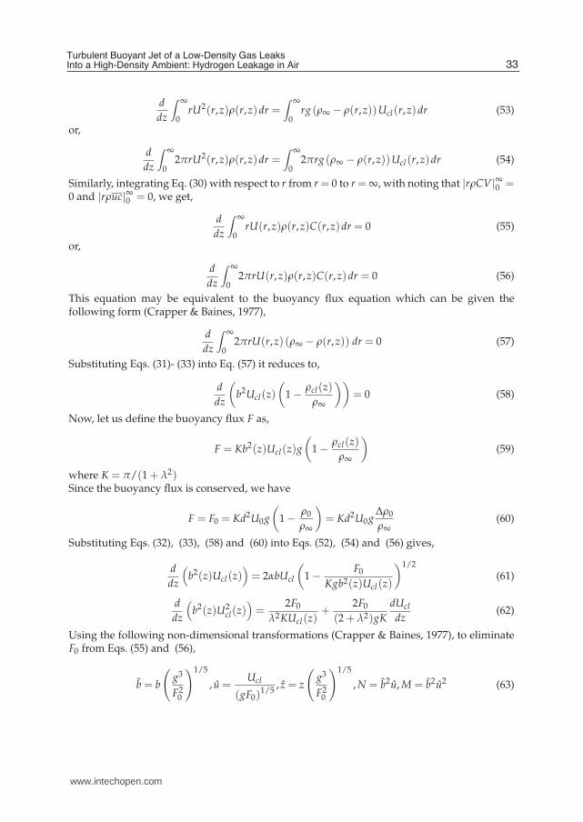
Now, let us integrate Eq. (29) with respect to r from r = 0 to r = ∞, with noting that |rρUV|∞0 =0 and |rρuv|∞0 = 0, we get,


www.intechopen.com


d

dz

∫

∞

0rU2(r,z)ρ(r,z)dr =

∫

∞

0rg (ρ∞ − ρ(r,z))Ucl(r,z)dr (53)

or,

d

dz

∫

∞

02πrU2(r,z)ρ(r,z)dr =

∫

∞

02πrg (ρ∞ − ρ(r,z))Ucl(r,z)dr (54)

Similarly, integrating Eq. (30) with respect to r from r = 0 to r = ∞, with noting that |rρCV|∞0 =0 and |rρuc|∞0 = 0, we get,

d

dz

∫

∞

0rU(r,z)ρ(r,z)C(r,z)dr = 0 (55)

or,

d

dz

∫

∞

02πrU(r,z)ρ(r,z)C(r,z)dr = 0 (56)

This equation may be equivalent to the buoyancy flux equation which can be given thefollowing form (Crapper & Baines, 1977),

d

dz

∫

∞

02πrU(r,z) (ρ∞ − ρ(r,z)) dr = 0 (57)

Substituting Eqs. (31)- (33) into Eq. (57) it reduces to,

d

dz

(

b2Ucl(z)

(

1 − ρcl(z)

ρ∞

))

= 0 (58)

Now, let us define the buoyancy flux F as,

F = Kb2(z)Ucl(z)g

(

1 − ρcl(z)

ρ∞

)

(59)

where K = π/(1 + λ2)Since the buoyancy flux is conserved, we have

F = F0 = Kd2U0g

(

1 − ρ0

ρ∞

)

= Kd2U0gΔρ0

ρ∞

(60)

Substituting Eqs. (32), (33), (58) and (60) into Eqs. (52), (54) and (56) gives,

d

dz

(

b2(z)Ucl(z))

= 2αbUcl

(

1 − F0

Kgb2(z)Ucl(z)

)1/2

(61)

d

dz

(

b2(z)U2cl(z)

)

=2F0

λ2KUcl(z)+

2F0

(2 + λ2)gK

dUcl

dz(62)

Using the following non-dimensional transformations (Crapper & Baines, 1977), to eliminateF0 from Eqs. (55) and (56),

b = b

(

g3

F20

)1/5

, u =Ucl

(gF0)1/5

, z = z

(

g3

F20

)1/5

, N = b2u, M = b2u2 (63)


www.intechopen.com

16 Mass Transfer

where b, u, z are known as top-hat variable (Thomas, 1963; Rooney & Linden, 1996) and aredefined respectively as dimensionless radius, centerline velocity and vertical coordinate ofthe plume. N and M are the dimensionless mass and momentum respectively. Using thetransformations (63), Eqs. (61) and (62) can be given in the form,

dN

dz= 2αM1/2

(

1 − 1

KN

)1/2

(64)

dM

dz=

(

1

KN − A

)

(

2N

λ2 M− 2αA

M3/2

N

(

1 − 1

KN

)1/2)

(65)

where A = 2/(2 + λ2).The corresponding initial conditions are,

N0 =1

(K(ρ∞ − ρ0)/ρ∞), M0 =

(

U20 /gb0

)2/5

(K(ρ∞ − ρ0)/ρ∞)6/5(66)

It is common in literature to use the dimensionless height z/d to express the jet travelingdistance from the source; so it will be more convenience to do the same in the current study.Using formulas (63), we can obtain the following relation between z and z,

z

d=

z

b0

=z√

M0

N0(67)

Also, the dimensionless centerline velocity and the jet/plume width can be related to theirtop-hat variables by the following relations,

b

d=

b

b0

=N

N0

√

M0

M(68)

Ucl

U0=

u

u0=

M

M0

N0

N(69)

3.4 Centerline quantities

In order to determine of the centerline quantities, the above non-linear first order ordinarydifferential system (64)- (65) with the associated initial conditions (66) are integratednumerically. With the aid of the above definition of the buoyancy flux F as well as therelation between density and mass fraction the centerline velocity and jet width and thereforecenterline density and centerline concentration can be determined. The solutions are obtainedfor hydrogen-air buoyant jet, for various values of Froude number Fr = 99 (U0 = 49.7),Fr = 152 (Fr = 76) and Fr = 268 (U0 = 134); as used for experiments by (Houf & Schefer,2008; Schefer et al., 2008a), at d = 0.00191, λ = 0.83, and Δρ0/ρ∞ = 0.93. The entrainmentcoefficient α is considered as a variable given by Eq. (41). The centerline hydrogen massfraction Ccl for H2-air jet at Fr = 99, Fr = 152 and Fr = 268 are plotted in Fig.7 and comparedwith the theoretical asymptotic limits for momentum-dominated jets (1/Ccl ∝ z) and thebuoyancy-dominated plume limit (1/Ccl ∝ z5/3).


www.intechopen.com


0.001

0.01

0.1

1

1 10 100 1000

Ccl (m

ass f

racti

on

)

z/d

Fr=99 Fr=152

Fr=268

Plume Theory:

Jet Theory:

Fig. 7. Comparison of the current model and jet theory of the centerline mass fraction(log-log plot) for H2 − Air jet, with different values of Froude number.

Fig. 8. Contours of the mean mole fraction for H2 − Air jet with different values of Froudenumber, with different values of Froude number.


www.intechopen.com

18 Mass Transfer

3.5 Mean quantities

Using the mean centerline quantities obtained above with the Gaussian profiles assumptionsof axial velocity, density deficiency and mass fraction, Eqs. (31)- (33), we can create a mapof the jet concentration and velocity. Using the relation between the mass fraction, molefraction and density, contours of mole fraction concentration are plotted in Fig.8. Fig. 9shows a comparison between the present calculations and experiments results (Schefer et al.,2008b) for radial profiles of the mean mass fraction concentration at several axial locationsfor momentum-dominated (Fr = 268) H2 − Air jet. The maximum centerline mass fraction ateach axial location occurs and decreases outward toward the surrounding air. Also, the samefigure indicates that the centerline concentration decreases in the downstream direction dueto mixing with the ambient air.Variations of the normalized mean density across the He-Air jet for axial locations from z/d =50 to 120 and compared with the experimental results by (Panchapakesan & Lu, 1993) at d =0.00612, λ = 0.84, and Δρ0/ρ∞ = 0.86 are shown in Fig.10. The maximum deviation of thepresent model from the experimental results in (Panchapakesan & Lu, 1993) is around 4% forthe normalized density. It is worth mentioning that for He− Air jet the entrainment coefficientis taken as a constant while it is considered as a variable as explained above for calculationsof H2 − Air jet. The mean cross-stream velocity can be obtained by solving the continuityequation for the time-averaged velocities by substituting from (33) and (32) into (28). Fig.12shows the normalized cross-stream velocity profiles V/Ucl plotted against the normalizedcoordinate r/cz for H2 − Air jet with various values of Froude number Fr = 268, 152 and 99.It can be seen from this figure that the cross-stream velocity vanishes at the centerline andbecomes outward in the neighborhood of the centerline. A maximum is then reached, thendeclines back to zero and then becomes inward (V/Ucl < 0), reaches a minimum and reachesan asymptote of zero as r/cz → ∞. The cross-stream velocity asymptotes to zero much moreslowly than the streamwise velocity does, thus, the central region is dominated by the axialcomponent of velocity, while the cross-stream flow predominates far away from it. Also,

0

0.02

0.04

0.06

0.08

0.1

0.12

0.14

0 2 4 6 8 10 12 14 16

C(r

,z)_

mass f

racti

on

r/d

Present, z/d=10 Present, z/d=25

Present, z/d=50 Present, z/d=100

Exp., z/d=10 Exp., z/d=25

Exp., z/d=50 Exp., z/d=100

Fr=268

Fig. 9. Radial profiles of the mean mass fraction for momentum-dominated (Fr=268) H2 − Airjet at several axial locations, compared with experimental results (Schefer et al., 2008b).


www.intechopen.com


0.84

0.88

0.92

0.96

1

0 0.05 0.1 0.15 0.2 0.25r/z

z/d=50

z/d=80

z/d=100

z/d=120

z/zzz d=50

z/d=====80

z/d=10000

z/d=dd 120

0.

Fig. 10. Radial profiles of the normalized mean density deficiency for He − Air jet at severalaxial locations. Dots refer to experimental results (Panchapakesan & Lu, 1993) at axiallocations from z/d=50 to 120.

Fig.11 indicates that as Froude number decreases and the distance from source increases thespreading rate increases and therefore the outward velocity increases.

3.6 Selected turbulent quantities

In this section, we determine some of the most important turbulent quantities such asReynolds stress, velocity-concentration correlation, etc. By substituting the time-averaged

-0.02

-0.01

0

0.01

0.02

0.03

0 1 2 3 4 5

V/U

cl

r/cz

Fr=99, z/d=25 Fr=99, z/d=100

Fr=152, z/d=25 Fr=152, z/d=100

Fr=268, z/d=25 Fr=268, z/d=100

Fig. 11. Radial profiles of the mean cross-stream velocity of H2 − Air jet with different valuesof Froude number at several axial locations.


www.intechopen.com

20 Mass Transfer

profiles of U, ρ and V obtained above into the momentum equation (29), we obtain thetime-averaged profile for the Reynolds stress uv. The radial profiles of normalized Reynoldsstress are plotted against the normalized coordinate r/cz at several axial locations for H2 − Airjet with various values of Froude number Fr = 268, 152 and 99, as shown in Fig.12. It isobserved from this figure that the Reynolds stress uv/U2

cl increases as the Froude numberdecreases due to increasing of jet spreading rate.Again, the time-averaged profile for the velocity-concentration correlation (radial flux) vcis determined by inserting the time-averaged profiles of U, ρ and C into the concentrationequation (30). The radial profiles of normalized velocity-concentration correlation are plottedin Fig.13 against the normalized coordinate r/cz at several axial locations for H2 − Air jetwith various values of Froude number Fr = 268, 152 and 99. This figure indicates that thevelocity-concentration correlation increases as the Froude number decreases. The turbulenteddy viscosity νt is related to Reynolds stress and the mean axial velocity by the relation,

uv = −νt∂U

∂r(70)

while, the turbulent eddy diffusivity Dt are related to the radial flux and the meanconcentration by the relation,

vc = −Dt∂C

∂r(71)

Using current calculation we can determine the turbulent eddy viscosity νt and turbulenteddy diffusivity Dt. Also, both the normalized turbulent eddy viscosity νt/Uclb, and thenormalized turbulent eddy diffusivity Dt/Uclb, are plotted in Fig.14 against the normalizedcoordinate r/cz at several axial locations for momentum-dominated H2 − Air jet (Fr = 268).Fig.14 illustrates that both νt/Uclb and Dt/Uclb have maximum values at the centerline ofthe jet and decay to zero for large r. If the effects of molecular transport are neglected,the turbulent Schmidt number in the free turbulent flow may be defined as the quantitativedifference between the turbulent transport rate of material and momentum. In other words,the turbulent Schmidt number, Sct = νt Dt, is a ratio of the eddy viscosity of the turbulent flow

0

0.005

0.01

0.015

0.02

0.025

0.03

0.035

0 0.5 1 1.5 2 2.5 3r/cz

Fr=99, z/d=50

Fr=99, z/d=100

Fr=152, z/d=50

Fr=152, z/d=100

Fr=268, z/d=50

Fr=268, z/d=100

0

0

Fig. 12. Radial profiles of the Reynolds stress for H2 − Air jet with different values of Froudenumber at several axial locations.


www.intechopen.com


0

0.005

0.01

0.015

0.02

0.025

0.03

0.035

0.04

0 0.5 1 1.5 2 2.5 3r/cz

Fr=99, z/d=50

Fr=99, z/d=100

Fr=152, z/d=50

Fr=152, z/d=100

Fr=268, z/d=50

Fr=268, z/d=100

Fig. 13. Radial profiles of the velocity-concentration correlation for H2 − Air jet with differentvalues of Froude number at several axial locations.

νt to the eddy material diffusivity Dt. It is very well known from literature that the spreadingrate of material in free jets is greater than that of momentum; thus, the turbulent Schmidtnumber is less than unity and has a significant effect on the predictions of species spreadingrate in jet flows. The turbulent eddy viscosity νt and the turbulent eddy diffusivity Dt, givethe turbulent Schmidt number as,

Sct =νt

Dt(72)

0.01

0.02

0.03

0.04

0.1 0.4 0.7 1 1.3r/cz

Fr=268

z/d=50,75, 100

El-Amin & Kanayama (2009 )

Fig. 14. Radial profiles of turbulent eddy viscosity and turbulent eddy diffusivity forH2 − Air with Fr = 268 (momentum-dominated) at several axial locations, compared with(El-Amin, 2009).


www.intechopen.com

22 Mass Transfer

0.7

0.8

0.9

1

1.1

1.2

1.3

0 0.2 0.4 0.6 0.8 1

Sct

r/cz

Fr=99, z/d=25 Fr=99, z/d=100

Fr=152, z/d=25 Fr=152, z/d=100

Fr=268, z/d=25 Fr=268, z/d=100

Fig. 15. Radial profiles of turbulent Schmidt number for H2 − Air jet with different values ofFroude number at several axial locations.

Turbulent Schmidt number is plotted in Fig.15 against the normalized coordinate r/cz atseveral axial locations for H2 − Air jet with various values of Froude number Fr = 268, 152 and99. In the momentum-dominated region the turbulent Schmidt number seems to be constantand the opposite is true when the buoyancy effects take place for small Froude number orfar distance from the jet source. Irrespective of the turbulence structure, the constant valueof the turbulent Schmidt number across the whole flow field implies that the momentumprocess is similar to the material-transport process. The opposite is true for the variable valuesof the turbulent Schmidt number indicate that the momentum process is not similar to thematerial-transport process. Now, let us define the normalized streamwise momentum fluxdensity across an isothermal jet as, G = (U/Ucl)

2, and the normalized jet-feed material densityas, W = UC/UclCcl . Also, by considering the analytical correlation of jet-feed concentration

and streamwise velocity derived by (El-Amin & Kanayama, 2009b) as, W = G(1 + Sct)/2 (seeFig.6).

4. References

Agrawal, A. & Prasad, A. K. (2002). Properties of vortices in the self-similar turbulent jet, Exp.Fluids 33: 565–577.

Agrawal, A. & Prasad, A. K. (2003). Integral solution for the mean flow profiles of turbulentjets, plumes, and wakes, ASME J Fluids Engineering 125: 813–822.

Batchelor, G. K. (1954). Heat convection and buoyancy effects in fluids, Q. J. R. Met. Soc.80: 339–358.

Becker, H. A., Hottel, H. C. & Williams, G. C. (1967). The nozzle-fluid concentration of theround turbulent free jet, J. Fluid Mech 30: 285–303.

Bhat, G. S. & Krothapalli, A. (2000). Simulation of a round jet and a plume in a regionalatmospheric model, Monthly Weather Review 128: 4108–4117.

Bhat, G. S. & Narasimha, R. A. (1996). A volumetrically heated jet: Large-eddy structure and


www.intechopen.com


entrainment characteristics, J. Fluid Mechanics 325: 303–330.Carlotti, P. & Hunt, G. R. (2005). Analytical solutions for turbulent non-boussinesq plumes, J.

Fluid Mechanics 538: 343–359.Chen, C. J. & Rodi, W. (1980). Vertical turbulent buoyant jets – a review of experimental data,

Pergamon Press, Oxford, UK.Crapper, P. F. & Baines, W. D. (1977). Non-boussinesq forced plumes, Atmospheric Environment

11: 415–420.Dai, Z., Tseng, L. K. & Faeth, G. M. (1995). Velocity statistics of round, fully developed,

buoyant turbulent plumes, Trans. ASME, J. Heat Transfer 117: 138–145.El-Amin, M. F. (2009). Non-boussinesq turbulent buoyant jet resulting from hydrogen leakage

in air, Int. J. Hydrogen Energy 34: 7873–7882.El-Amin, M. F., Inoue, M. & H., K. (2008). Boundary layer theory approach to the concentration

layer adjacent to a ceiling wall of a hydrogen leakage: far region, Int. J. HydrogenEnergy 33: 7642–7647.

El-Amin, M. F. & Kanayama, H. (2008). Boundary layer theory approach to the concentrationlayer adjacent to a ceiling wall at impinging region of a hydrogen leakage, Int. J.Hydrogen Energy 33: 6393–6400.

El-Amin, M. F. & Kanayama, H. (2009a). Boundary layer theory approach to the concentrationlayer adjacent to the ceiling wall of a hydrogen leakage: axisymmetric impinging andfar regions, Int. J. Hydrogen Energy 34: 1620–1626.

El-Amin, M. F. & Kanayama, H. (2009b). Integral solutions for selected turbulent quantities ofsmall-scale hydrogen leakage: a non-buoyant jet or momentum-dominated buoyantjet regime, Int. J. Hydrogen Energy 34: 1607–1612.

El-Amin, M. F. & Kanayama, H. (2009c). Similarity consideration of the buoyant jet resultingfrom hydrogen leakage, Int. J. Hydrogen Energy 34: 5803–5809.

El-Amin, M. F., Sun, S., Heidemann, W. & Mller-Steinhagen, H. (2010). Analysis of aturbulent buoyant confined jet using realizable k-¡ep¿ model, Heat and Mass TransferTo appear: 1–20.

Fischer, H. B., List, E. J., Koh, R. C. Y., Imberger, J. & Brooks, N. H. (1979). Mixing in Inland andCoastal Waters, Academic Press.

Gebhart, B., Jaluria, Y., Mahajan, R. L. & Sammakia, B. (1988). Buoyancy-induced flows andtransport, Hemisphere. Washington, DC.

He, G., Yanhu, G. & A., H. (1999). The effect of schmidt number on turbulent scalar mixing ina jet-in-cross flow, Int. J. Heat Mass Transfer 42: 3727–3738.

Hinze, J. O. (1975). Turbulence, 2nd ed., McGraw-Hill.Hirst, E. A. (1971). Analysis of buoyant jets within the zone of flow establishment, Technical

report, Oak Ridge National Laboratory, Report ORNL-TM-3470.Houf, W. G. & Schefer, R. W. (2007). Predicting radiative heat fluxes and flammability

envelopes from unintended releases of hydrogen, Int. J. Hydrogen Energy 32: 136–151.Houf, W. G. & Schefer, R. W. (2008). Analytical and experimental investigation of small-scale

unintended releases of hydrogen, Int. J. Hydrogen Energy 33: 1435–1444.Hussein, J. H., Capp, S. P. & George, W. K. (1994). Velocity measurements in a

high-reynolds-number, momentum-conserving, axisymmetric, turbulent jet, J. FluidMechanics 258: 31–75.

Lessen, M. (1978). On the power laws for turbulent jets, wakes and shearing layers and theirrelationship to the principal of marginal instability, J. Fluid Mech 88: 535–540.

List, E. J. (1982). Turbulent jets and plumes, Annual Review of Fluid Mechanics 14: 189–212.


www.intechopen.com

24 Mass Transfer

Morton, B. R. (1965). Modelling fire plumes, 10th Int. Symposium on Combustion, 844-859.Panchapakesan, N. R. & Lu (1993). Turbulence measurements in axisymmetric jets of air and

helium. part 2. helium jet, J. Fluid Mechanics 246: 225–247.Panchapakesan, N. R. & Lumley, J. L. (1993). Turbulence measurements in axisymmetric jets

of air and helium. part 1. air jet, J. Fluid Mechanics 246: 197–223.Papantoniou, D. & List, E. J. (1989). Large-scale structure in the far field of buoyant jets, J.

Fluid Mechanics 209: 151–190.Rajaratnam, N. (1976). Turbulent Jets, Elsevier Science, Place of publication.Ricou, F. & Spalding, D. B. (1961). Measurements of entrainment by axisymmetrical turbulent

jets, J. Fluid Mechanics 8: 21–32.Rooney, G. G. & Linden, P. F. (1996). Similarity considerations for non-boussinesq plumes in

an unstratified environment, J. Fluid Mechanics 318: 237–250.Schefer, R. W., Houf, W. G., Bourne, B. & Colton, J. (2006). Spatial and radiative properties of

an open-flame hydrogen plume, Int. J. Hydrogen Energy 31: 1332–1340.Schefer, R. W., Houf, W. G. & Williams, T. C. (2008a). Investigation of small-scale unintended

releases of hydrogen: buoyancy effects, Int. J. Hydrogen Energy 33: 4702–4712.Schefer, R. W., Houf, W. G. & Williams, T. C. (2008b). Investigation of small-scale

unintended releases of hydrogen: momentum-dominated regime, Int. J. HydrogenEnergy 33: 6373–6384.

Shabbir, A. & Georg, W. K. (1994). Experiment on a round turbulent plume, J. Fluid Mechanics275: 1–32.

Spiegel, E. A. & Veronis, G. (1960). On the boussinesq approximation for a compressible fluid,Astrophys. J. 131: 442–447.

Steward, F. R. (1970). Prediction of the height of turbulent diffusion buoyant flames, Combust.Sci. Technol. 2: 203–212.

Swain, M. R., Filoso, P. A. & Swain, M. N. (2007). An experimental investigation into theignition of leaking hydrogen, Int. J. Hydrogen Energy 32: 287–295.

Takeno, K., Okabayashi, K., Kouchi, A., Nonaka, T., Hashiguchi, K. & Chitose, K. (2007).Dispersion and explosion field tests for 40 mpa pressurized hydrogen, Int. J. HydrogenEnergy 32: 2144–2153.

Tennekes, H. & Lumley, J. L. (1972). A First Course in Turbulence, MIT Press, Cambridge, MA.Thomas, P. H. (1963). The size of flames from natural fires, 9th Symposium on Combustion,

844-859.Townsend, A. A. (1966). The mechanism of entrainment in free turbulent flows, J. Fluid

Mechanics 26: 689–715.Turner, J. S. (1973). Buoyancy effects in fluids, Cambridge Univ. Press, London.Turner, J. S. (1986). Turbulent entrainment: The development of the entrainment assumption,

and its application to geophysical flows, J. Fluid Mech 173: 431–471.Venkatakrishnan, L., Bhat, G. S. & Narasimha, R. (1999). Experiments on plume

with off-source heating: Implications for cloud fluid dynamics, J. Geophys. Res.104: 14271–14281.

Woods, A. W. (1997). A note on non-boussinesq plumes in an incompressible stratifiedenvironment, J. Fluid Mechanics 345: 347–356.

Yimer, I., Campbell, I. & Jiang, L. Y. (2002). Estimation of the turbulent schmidt number fromexperimental profiles of axial velocity and concentration for high-reynolds-numberjet flows, Canadian Aeronautics Space Journal 48: 195–200.


www.intechopen.com

Advanced Topics in Mass TransferEdited by Prof. Mohamed El-Amin

ISBN 978-953-307-333-0Hard cover, 626 pagesPublisher InTechPublished online 21, February, 2011Published in print edition February, 2011

InTech EuropeUniversity Campus STeP Ri Slavka Krautzeka 83/A 51000 Rijeka, Croatia Phone: +385 (51) 770 447 Fax: +385 (51) 686 166www.intechopen.com

InTech ChinaUnit 405, Office Block, Hotel Equatorial Shanghai No.65, Yan An Road (West), Shanghai, 200040, China

Phone: +86-21-62489820 Fax: +86-21-62489821

This book introduces a number of selected advanced topics in mass transfer phenomenon and covers itstheoretical, numerical, modeling and experimental aspects. The 26 chapters of this book are divided into fiveparts. The first is devoted to the study of some problems of mass transfer in microchannels, turbulence, wavesand plasma, while chapters regarding mass transfer with hydro-, magnetohydro- and electro- dynamics arecollected in the second part. The third part deals with mass transfer in food, such as rice, cheese, fruits andvegetables, and the fourth focuses on mass transfer in some large-scale applications such as geomorphologicstudies. The last part introduces several issues of combined heat and mass transfer phenomena. The bookcan be considered as a rich reference for researchers and engineers working in the field of mass transfer andits related topics.

How to referenceIn order to correctly reference this scholarly work, feel free to copy and paste the following:

M.F. El-Amin and Shuyu Sun (2011). Turbulent Buoyant Jet of a Low-Density Gas Leaks into High-DensityAmbient: Hydrogen Leakage in Air, Advanced Topics in Mass Transfer, Prof. Mohamed El-Amin (Ed.), ISBN:978-953-307-333-0, InTech, Available from: http://www.intechopen.com/books/advanced-topics-in-mass-transfer/turbulent-buoyant-jet-of-a-low-density-gas-leaks-into-high-density-ambient-hydrogen-leakage-in-air

© 2011 The Author(s). Licensee IntechOpen. This chapter is distributedunder the terms of the Creative Commons Attribution-NonCommercial-ShareAlike-3.0 License, which permits use, distribution and reproduction fornon-commercial purposes, provided the original is properly cited andderivative works building on this content are distributed under the samelicense.

https://creativecommons.org/licenses/by-nc-sa/3.0/

Documents

Turbulent Buoyant Jet of a Low-Density Gas Leaks Into a High