Turbulence-Flame Interactions in Type Ia Supernovae

A. J. Aspden1, J. B. Bell1, M. S. Day1, S. E. Woosley2, and M. Zingale3

ABSTRACT

The large range of time and length scales involved in type Ia supernovae (SN

Ia) requires the use of flame models. As a prelude to exploring various options

for flame models, we consider, in this paper, high-resolution three-dimensional

simulations of the small-scale dynamics of nuclear flames in the supernova envi-

ronment in which the details of the flame structure are fully resolved. The range

of densities examined, 1 to 8×107 g cm−3, spans the transition from the laminar

flamelet regime to the distributed burning regime where small scale turbulence

disrupts the flame. The use of a low Mach number algorithm facilitates the ac-

curate resolution of the thermal structure of the flame and the inviscid turbulent

kinetic energy cascade, while implicitly incorporating kinetic energy dissipation

at the grid-scale cutoff. For an assumed background of isotropic Kolmogorov

turbulence with an energy characteristic of SN Ia, we find a transition density

between 1 and 3 × 107 g cm−3 where the nature of the burning changes qual-

itatively. By 1 × 107 g cm−3, energy diffusion by conduction and radiation is

exceeded, on the flame scale, by turbulent advection. As a result, the effective

Lewis Number approaches unity. That is, the flame resembles a laminar flame,

but is turbulently broadened with an effective diffusion coefficient, DT ∼ u′l,

where u′ is the turbulent intensity and l is the integral scale. For the larger

integral scales characteristic of a real supernova, the flame structure is predicted

to become complex and unsteady. Implications for a possible transition to deto-

nation are discussed.

Subject headings: supernovae: general — white dwarfs — hydrodynamics —

nuclear reactions, nucleosynthesis, abundances — conduction — methods: nu-

merical — turbulence

1Lawrence Berkeley National Laboratory, 1 Cyclotron Road, MS 50A-1148, Berkeley, CA 94720

2Department of Astronomy and Astrophysics, University of California at Santa Cruz, Santa Cruz, CA

95064

3Department of Physics and Astronomy, Stony Brook University, Stony Brook, NY 11794

– 2 –

1. INTRODUCTION

The complex small-scale dynamics of turbulent thermonuclear flames are essential to

understanding SN Ia. Since the range of length scales is so large (star size ∼ 108 cm;

Kolmogorov scale and flame thickness < 1 mm), full star calculations must use a subgrid

model to describe the burning on the unresolved scales. Turbulent flame models (Niemeyer

& Hillebrandt 1995) that move the flame at the turbulent velocity have been successful at

producing explosions (Ropke & Hillebrandt 2005) with pure deflagrations. Another popular

flame model (Khokhlov 1991) moves the flame at the speed dictated by the Rayleigh-Taylor

instability, and has also produced successful explosions (Gamezo et al. 2003), although the

authors argue that a more realistic supernova is produced when a detonation ensues late in

the explosion (Gamezo et al. 2005). These two flame models can produce large differences

in the flame speeds at small scales, which will have a large effect on the outcome of full-

star simulations. Validation of these models against resolved flame calculations is needed to

resolve this discrepancy.

As the flame propagates outward from the center of the star, it encounters lower den-

sities, the speed decreases, and the flame thickens. A critical length scale in turbulent

combustion is the Gibson scale – the length scale at which the laminar flame speed equals

the turbulent velocity (see for example Peters 2000),

lG = l(sL

u′

)3

. (1)

Here sL is the laminar flame speed, and u′ and l are velocity and integral length scales

characterizing the turbulence, and we have assumed Kolmogorov scaling. At a density of

around 107 g cm−3, the flame becomes thick enough that turbulent eddies can disrupt its

structure before they burn away (Niemeyer & Woosley 1997), that is, the flame thickness is

larger than the Gibson scale. At this point, the burning fundamentally changes character

and the flame is said to be in the distributed burning regime (see Peters 2000 for some

discussion).

Here we look at the interaction of the flame and turbulence on the scale of the flame,

with the aim of validating turbulent flame models and better understanding the transition to

distributed burning. Previous studies of flames interacting with turbulence have focused on

flames interacting with vortical flow (two-dimensional simulations presented in Ropke et al.

2004) or statistical methods using one-dimensional turbulence (Lisewski et al. 2000a,b). An

open question is whether in the distributed burning regime, a mixed region of partially

burned fuel and ash can grow large enough such that it can ignite a detonation (Niemeyer

& Woosley 1997; Khokhlov et al. 1997; Niemeyer 1999). Detonations have gained renewed

interest lately as a means to burn the carbon/oxygen fuel left behind near the center of

– 3 –

the white dwarf in pure deflagration models (Gamezo et al. 2005). Although, it is unclear

whether detonations can traverse the pockets of partially burned fuel (Golombek & Niemeyer

2005). Recent results also suggest that the size of the region of partially burned fuel needed

to initiate a detonation is larger than previously believed (Dursi & Timmes 2006). Pan et al.

(2008) discusses the role of turbulent intermittency on the conditions needed for transition

to detonation.

Previously, we showed the transition to the distributed burning regime in two dimensions

(Bell et al. 2004b), where the Rayleigh-Taylor instability (RT), growing on scales smaller

than the flame thickness itself, is responsible for the transition. It has been suggested

(Niemeyer & Kerstein 1997) that turbulence generated by RT in type Ia supernovae should

obey Bolgiano-Obukhov (BO) statistics – formulated from considering a potential energy

cascade. However, recently is was shown that BO scaling only applies in two-dimensions

(Chertkov 2003; Zingale et al. 2005a). Three-dimensional RT-unstable flame calculations

have shown that turbulence is indeed Kolmogorov in nature and becomes isotropic on the

small scales (Zingale et al. 2005b; Cabot & Cook 2006). As first discussed in Niemeyer &

Kerstein (1997), BO scaling leads to a lower transition to distributed burning, and therefore,

makes a detonation transition more difficult. Therefore, although our two-dimensional results

led us to conclude that a DDT was unlikely (Bell et al. 2004b), a three-dimensional study is

warranted.

Figure 1 shows how the relevant length scales vary with fuel density. In particular, the

two red curves compare the laminar flame width and the Gibson scale. The laminar flame

widths have been calculated from simulated one-dimensional profiles. The Gibson scale is

evaluated assuming a turbulent intensity, u∗, of 107 cm s−1 on a length scale, L∗, of 106 cm, as

in Niemeyer & Woosley (1997). We see that the transition to distributed burning, assuming

Kolmogorov turbulence, should occur around 3 × 107 g cm−3.

In this paper, we present a three-dimensional study of turbulent thermonuclear flames

that explores a range of conditions from the flamelet regime to the distributed burning

regime. Specifically, we use a flame sheet embedded in a maintained turbulent velocity

field. Of particular interest is the response of the flames to wrinkling by the turbulence, and

the scaling of the turbulent flame speed with the turbulent intensity. Thermal diffusion is

orders of magnitude greater than species diffusion (the Lewis number is large) (Timmes &

Woosley 1992) and has a significant effect on the turbulence-flame interactions. Attention

is then focused on the distributed burning regime and potential implications for a transition

to detonation are discussed.

– 4 –

2. SIMULATION DESCRIPTION

We use a low Mach number hydrodynamics code, adapted to the study of thermonuclear

flames, as described in Bell et al. (2004a). The advantage of this method is that sound waves

are filtered out analytically, so the time step is set by the the bulk fluid velocity and not the

sound speed. This is an enormous efficiency gain for low speed flames. The input physics

used in the present simulations is largely unchanged, with the exception of the addition of

Coulomb screening, taken from the Kepler code (Weaver et al. 1978), to the 12C(12C,γ)24Mg

reaction rate. This yields a small enhancement to the flame speed, and is included for

completeness. The conductivities are those reported in Timmes (2000), and the equation of

state is the Helmholtz free-energy based general stellar EOS described in Timmes & Swesty

(2000). We note that we do not utilize the Coulomb corrections to the electron gas in the

general EOS, as these are expected to be minor in the conditions considered.

The non-oscillatory finite-volume scheme employed here permits the use of implicit

large eddy simulation (iles). This technique captures the inviscid cascade of kinetic energy

through the inertial range, while the numerical error acts in a way that emulates the phys-

ical effects of the dynamics at the grid scale, without the expense of resolving the entire

dissipation subrange. The approach was introduced by Boris et al. (1992), and has since

been used by many authors (e.g. Youngs (1991), Porter et al. (1992), Grinstein & Fureby

(2004), and Margolin et al. (2006)). An overview of the technique can be found in Grinstein

et al. (2007). Aspden et al. (2008) presented a detailed study of the technique using the

present numerical scheme, including a characterization that allowed for an effective viscosity

to be derived. Thermal diffusion plays a significant role in the flame dynamics, and so is

explicitly included in the model, whereas species diffusion is significantly smaller, and so is

not explicitly included.

The turbulent velocity field was maintained using a forcing term similar to that used in

the study of Aspden et al. (2008). Specifically, a forcing term was included in the momen-

tum equations consisting of a superposition of long wavelength Fourier modes with random

amplitudes and phases. The forcing term is scaled by density so that the forcing is somewhat

reduced in the ash. This approach provides a way to embed the flame in a zero-mean turbu-

lent background, mimicking the much larger inertial range that these flames would experience

in a type Ia supernova, without the need to resolve the large-scale convective motions that

drive the turbulent energy cascade. Figure 2 shows an example kinetic energy wavenumber

spectrum taken from Aspden et al. (2008) at a resolution comparable to that used here; the

dashed line denotes a minus five-thirds decay, and is illustrative of the turbulence found in

the present study. Aspden et al. (2008) demonstrated that the effective Kolmogorov length

scale is approximately 0.28∆x, and the integral length scale is approximately a tenth of the

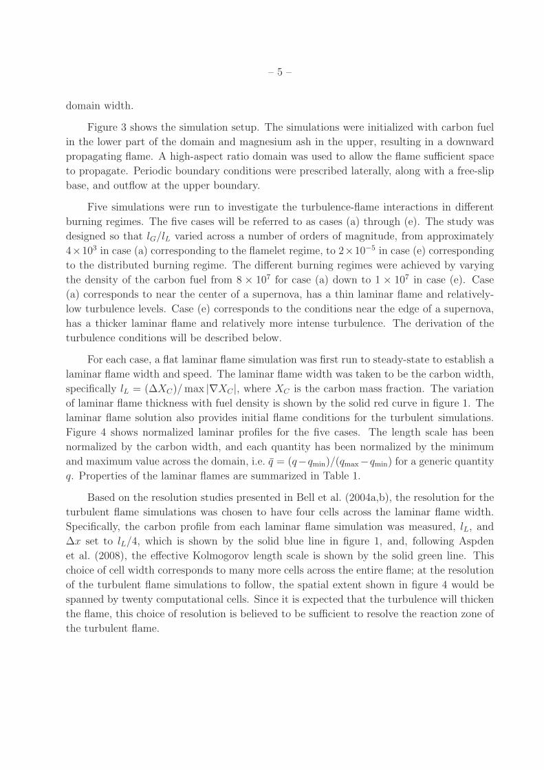
– 5 –

domain width.

Figure 3 shows the simulation setup. The simulations were initialized with carbon fuel

in the lower part of the domain and magnesium ash in the upper, resulting in a downward

propagating flame. A high-aspect ratio domain was used to allow the flame sufficient space

to propagate. Periodic boundary conditions were prescribed laterally, along with a free-slip

base, and outflow at the upper boundary.

Five simulations were run to investigate the turbulence-flame interactions in different

burning regimes. The five cases will be referred to as cases (a) through (e). The study was

designed so that lG/lL varied across a number of orders of magnitude, from approximately

4×103 in case (a) corresponding to the flamelet regime, to 2×10−5 in case (e) corresponding

to the distributed burning regime. The different burning regimes were achieved by varying

the density of the carbon fuel from 8 × 107 for case (a) down to 1 × 107 in case (e). Case

(a) corresponds to near the center of a supernova, has a thin laminar flame and relatively-

low turbulence levels. Case (e) corresponds to the conditions near the edge of a supernova,

has a thicker laminar flame and relatively more intense turbulence. The derivation of the

turbulence conditions will be described below.

For each case, a flat laminar flame simulation was first run to steady-state to establish a

laminar flame width and speed. The laminar flame width was taken to be the carbon width,

specifically lL = (∆XC)/ max |∇XC |, where XC is the carbon mass fraction. The variation

of laminar flame thickness with fuel density is shown by the solid red curve in figure 1. The

laminar flame solution also provides initial flame conditions for the turbulent simulations.

Figure 4 shows normalized laminar profiles for the five cases. The length scale has been

normalized by the carbon width, and each quantity has been normalized by the minimum

and maximum value across the domain, i.e. q = (q−qmin)/(qmax−qmin) for a generic quantity

q. Properties of the laminar flames are summarized in Table 1.

Based on the resolution studies presented in Bell et al. (2004a,b), the resolution for the

turbulent flame simulations was chosen to have four cells across the laminar flame width.

Specifically, the carbon profile from each laminar flame simulation was measured, lL, and

∆x set to lL/4, which is shown by the solid blue line in figure 1, and, following Aspden

et al. (2008), the effective Kolmogorov length scale is shown by the solid green line. This

choice of cell width corresponds to many more cells across the entire flame; at the resolution

of the turbulent flame simulations to follow, the spatial extent shown in figure 4 would be

spanned by twenty computational cells. Since it is expected that the turbulence will thicken

the flame, this choice of resolution is believed to be sufficient to resolve the reaction zone of

the turbulent flame.

– 6 –

Computational expense restricts the domain to a cross-section of 256 cells, and so, since

∆x is known, the domain width follows, and the forcing term determines the integral length

scale. The domain width and integral length scales are shown in figure 1 by the solid and

dashed black lines, respectively. It should be emphasized that the integral length scale

and effective Kolmogorov length scales are restricted by computational expense and are not

reflective of the values found in a supernova.

Turbulence characteristics can be estimated using a simple representation shear gener-

ation by the Rayleigh-Taylor instability. On the large scale of the supernova, the flame will

be unstable with a typical feature size of L∗ ∼ 106 cm. The velocity on this scale can be

estimated using the Sharp-Wheeler model (Sharp 1984),

u∗(L∗) ∼1

2

√

AtgL∗ . (2)

For an Atwood number, At ∼ 0.5 and gravitational acceleration, g ∼ 109 cm s−2, one has

u∗(L∗) ∼ 107 cm s−1, in agreement with the numbers used in Niemeyer & Woosley (1997).

More detailed simulations by Ropke (2007) in 3D find a distribution of turbulent intensities

peaking at 107 cm s−1, but with a high-velocity tail extending out to 108 cm s−1. For the

current simulations, the turbulent kinetic energy released by the large-scale RT motions is

assumed to cascade down to the flame scale following a Kolmogorov spectrum, as

u′(l) = u∗(L∗)

(

l

L∗

)1/3

, (3)

therefore, given the integral length scale, l, the turbulent velocity, u′(l), can be computed.

Throughout this paper, u∗ = 107 cm s−1 and L∗ = 106 cm have been assumed.

In cases (a)-(d), the aspect ratio of the domain was 4:1 and the flame placed one do-

main width from the upper boundary. In case (e) an aspect ratio of 8:1 was required to

accommodate the flame in the distributed burning regime, and the flame was initially placed

at the midpoint of the domain. In each case, adaptive mesh refinement was used to reduce

the computational expense. A base grid with 128 cells across was used, with one level of

amr with refinement factor 2 concentrated around the flame sheet. This gave an effective

resolution of 256 × 256 × 1024 for cases (a)-(d) and 256 × 256 × 2048 for case (e). Experi-

ments with additional resolution confirmed the adequacy of this choice. It was also ensured

that the use of amr had no detrimental effect on the turbulence. Specifically, the energy

containing scales were well captured by the base grid (see Aspden et al. (2008) for a study

of maintained homogeneous isotropic turbulence using the same approach) and there was

adequate refinement ahead of the flame to ensure that the cascade of energy to smaller scales

in the refined region (which have a short turn over time) could occur before these scales could

interact with the flame. Table 2 summarizes the properties of the turbulence simulations.

– 7 –

3. RESULTS

In each case, the flow undergoes an initial transition, as the turbulence wrinkles and

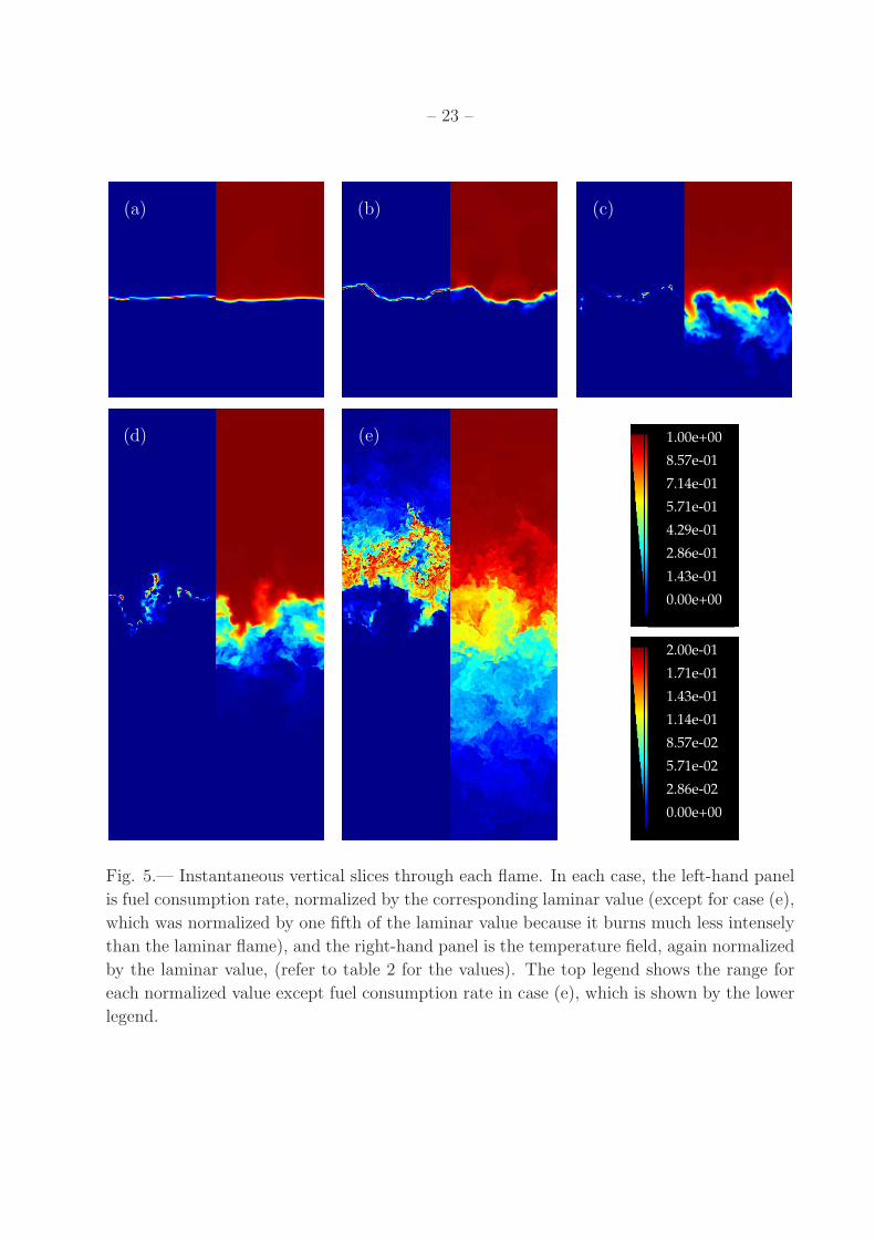
thickens the flame, until a quasi-steady state is established. Figure 5 shows instantaneous

vertical slices of fuel consumption rate (left panel) and temperature (right panel) for each

of the five cases once the quasi-steady state has been reached. In each case, the values have

been normalized by the corresponding laminar values, with the exception of case (e) where

the local fuel consumption rate is much lower and so has been normalized by a fifth of the

laminar value for contrast. By construction, the length scales are normalized by the laminar

flame width. Half of the domain is shown for cases (a)-(c) and case (e), and the entire

domain is shown for case (d).

Case (a) presents smooth and even burning, and is perturbed very little by the back-

ground turbulence. The temperature profile remains sharp. In case (b), the flame surface has

been deformed by the turbulence. Both regions of enhanced burning and regions of decreased

burning are observed, and appear to be correlated with the curvature of the flame sheet.

Specifically, enhanced burning appears to occur where the center of curvature is within the

fuel, and decreased when the center of curvature is in the ash. The temperature field presents

regions that are sharp, and regions that appear to be more diffuse. Again, this appears to

be correlated with curvature, with the more diffusive regions occurring where the center of

curvature is in the products.

In cases (c) and (d), as lG/lL decreases further, the background turbulence becomes

increasingly influential; the temperature field becomes more mixed, and the deformation of

the flame surface increases. The burning appears to occur in small high-intensity pockets,

punctuated by regions of local extinction.

In case (e), a dramatically different burning mode is observed. The temperature mixed

region and the burning region are much broader. The burning appears to be much less

intense (recall the image has been normalized by a fifth of the laminar value for contrast)

and is restricted to the high temperature end of the mixing zone. There is no well-defined

flame surface, but a broad flame brush. Interestingly, there appears to be some residual

low-level burning well above the main burning region, suggestive of incomplete burning in

the main flame zone.

These observations are further reinforced by three-dimensional renderings of the fuel

consumption rate, shown in figure 6, which elucidates the three-dimensional structure of the

flames. The images have been scaled in the same way as the corresponding slices. Case (a)

burns as a coherent connected flame sheet, but as the relative turbulence level increases in

cases (b) to (d), the flame sheet becomes increasingly disrupted and presents regions of local

– 8 –

extinction. Finally in case (e), in the distributed burning regime, the behavior is completely

different with a flame brush that is much broader but burns less intensely than the laminar

flame.

The curvature effects observed and the resulting burning rates are a consequence of the

thermo-diffusively-stable nature of the flames; the Lewis number is high – thermal diffusion

is much greater than species diffusion. Where the background turbulence elevates part of

the flame surface, resulting in negative curvature, there is a focusing of heat by diffusion.

Consequently, as the reaction rate is extremely sensitive to temperature, the fuel burns

quickly, and the flame is flattened. Conversely, where the turbulence pushes the flame

downwards, creating positive curvature, temperature diffusion leads to a defocusing of heat,

and the burning rate decreases. Again, this tends to flatten the flame. Curvature effects will

be explored further below.

The instantaneous global turbulent flame speed normalized by the laminar flame speeds

are shown in figure 7; the time scale is normalized by the laminar burning time – the time

it takes the laminar flame to burn one flame width. Note the different time axis for case

(e). Case (a) burns almost exactly at the the laminar flame speed. Curiously, cases (b) and

(c) actually burn more slowly overall than their laminar counterparts, and case (d) is only

around 30% faster. However, case (e) burns between approximately five and six times the

laminar flame speed.

To investigate the effects of curvature, it is useful to be able to define a flame surface.

There are a number of ways to do this, but it has been found that using isosurfaces of

temperature or fuel mass fraction is a practical way that avoids the difficulties associated

with the local extinction in these particular flames. We choose values for the isosurfaces

based on the temperature or fuel mass fraction values at the peak local fuel consumption

rate in the laminar flame. The isosurface was then located by using a standard “marching

cubes” algorithm, and optimized using the “QSlim” algorithm, see Garland (1999). Since

the temperature field is more diffusive than the fuel, the resulting isosurface was found to

be much smoother for temperature than the carbon, particularly where the isosurface was

within the fuel itself. Furthermore, because of the higher levels of turbulence in cases (d)

and (e), the isosurfaces were found to be too contorted to be useful.

Since the fuel consumption occurs over a finite width and is not localized to the flame

surface, a local consumption-based flame speed was evaluated by integrating the fuel con-

sumption rate through the surface. This involved constructing a set of integral curves along

the gradient vector of the progress variable through each point on the isosurface, ensuring

that the curves extended well beyond the region where the fuel consumption rate decreases

to zero. (We note that for this construction, we orient the normal to point into the ash.

– 9 –

With this orientation, the curvature, κ is negative when the center of curvature is in the

fuel.) These integral curves provided bounding edges of prism-shaped subvolumes that ef-

fectively cover the reaction zone. The consumption-based flame propagation speed was then

computed over each subvolume of the reaction zone by integrating the computed fuel con-

sumption rate over the subvolume. The local consumption-based flame speed was defined

as

slT =

1

ρ0XF,0A

∫

Ω

ρωF dΩ (4)

where ρ0XF,0 is the initial fuel density, Ω is the subvolume, ρωF is the local fuel consumption

rate, and A is the area of intersection of the flame with Ω. Defining the local speed in this

way has the property that the global burning speed is the integral of slT over the isosurface.

For additional detail about construction of the elements, Ω, see Bell et al. (2005).

Figure 8 compares instantaneous temperature and carbon isosurfaces for case (b), and

is colored by the integrated fuel consumption rate, slT . The correlation between burning rate

and curvature observed in figure 5 is more apparent here. Specifically, the regions of high fuel

consumption rate are strongly correlated with regions of negative curvature, i.e. where the

centers of curvature are within the fuel. Two examples are highlighted by arrows labeled ‘H’.

This correlation appears to differ slightly between the two isosurfaces. On the temperature

surface, there are regions of negative curvature where the burning is very low; two examples

are shown by arrows labeled ‘L’. However, the carbon surface does not appear to pass through

these regions; the labels are in the same place, but the carbon surface is much lower. The

temperature and carbon mass fraction have become decorrelated. Regions exists around the

peak burning temperature where there is no fuel, and so burning cannot occur. This is a

direct result of the competition between mixing by turbulence and thermal diffusion.

Figure 9 shows joint probability density functions (jpdf) of curvature (normalized by

the laminar flame width) and local integrated fuel consumption rate (normalized by the

laminar value), based on the temperature isosurface, ensemble-averaged over a number of

time-points after the flames have reached a quasi-steady state. The (negative) correlation

is clear and quantifies the between curvature and local flame speed observed above. It is

also evident that there is a significant change in burning across the three cases. Case (a)

shows that the majority of the fuel consumption occurs around the laminar rate. Case (b)

demonstrates that the flame is bimodal, in the sense that there are regions that are burning,

which are negatively correlated with curvature, but there are also regions of low burning or

local extinction, which occur with curvature of both signs. This suggests that where the

flame is burning, it is burning close to the laminar value (with low probability variability),

but because there are also regions of local extinction, the overall burning rate per unit area

is lower than the laminar value. Finally, in case (c), there is no preferred rate of burning, a

– 10 –

slight negative correlation with curvature, and significant regions of local extinction.

A common approach used for determining a model flame speed involves assuming that

the flame is burning locally at the laminar flame speed, and that global burning rate is equal

to the laminar flame speed times the area of the flame. Figure 10 shows the normalized

burning rate per unit area for cases (a-c). If the flame-modeling approach described above

was appropriate for these flames, this measure would be close to unity. This is indeed seen

to be the case for case (a), as the flame is burning in a very similar way to the laminar flame.

However, it is too simplistic an approximation for other two cases. The strong response

to curvature modulates the local burning speed. The values of approximately 0.8 and 0.5

suggest that using the laminar flame speed times the area of the flame would lead to an

overestimation of the global burning by factors of approximately 1.25 and 2 respectively.

The analysis indicates that even in the flamelet regime, a Markstein correction is needed to

predict the local flame speed accurately.

The way in which the burning occurs can be analyzed further by considering other joint

probability density functions. Figure 11 shows the jpdfs for all five cases of temperature and

carbon density, and figure 12 shows fuel consumption rate against temperature. Here the first

moment has been taken with respect to fuel consumption rate, specifically, for jpdf P (Q, T )

for fuel consumption rate Q and temperature T , the first moment is defined as QP (Q, T ).

This highlights the burning regions and prevent the large proportion of the domain that

is not burning from dominating the jpdf. Again, the pdfs have been ensemble-averaged.

The solid red line in each case denotes the laminar flame correlation. In case (a), it is clear

that the burning follows an almost identical path to the laminar flame. Case (b) present a

similar correlation, but there is greater variability around the main burning path. In cases

(c) and (d), the main burning path appears to have shifted away from the laminar flame, and

there is a large amount of variability from that main path. In case (e), a dramatic change is

observed, the burning path has collapsed to a single path that is significantly removed from

the laminar flame. In this case, the turbulent mixing dominates the thermal diffusion and

so the temperature and fuel cannot become decorrelated. Therefore, a single burning path

is observed, which is different than the laminar flame, with very little variability.

Figure 13 shows the joint probability density function of fuel consumption rate and

carbon mass fraction for case (e), again the first moment with respect to fuel consumption

rate has been taken to highlight the burning region. Similar to the corresponding temperature

plot, the burning path has collapsed to a curve that is significantly different than the laminar

flame and there is little variability around it. Importantly, this figure demonstrates that the

burning occurs at much lower mass fractions than in the laminar flame.

A normalized instantaneous flame structure in case (e) is compared with the laminar

– 11 –

flame structure in figure 14. The turbulent flame structure has been obtained by taking

planar averages. Here, the length scale has been normalized by the laminar flame carbon

width, and each of the other quantities has been normalized by the corresponding laminar

values, expect for the velocity, which has been normalized by the turbulent burning speed

due to its significantly enhanced value. The turbulent structure is dramatically different.

Note how the shape of the temperature and density profiles have changed, becoming closer

to hyperbolic tangents. In particular, the width of the temperature profile has decreased

relative to the carbon profile because the mixing is dominated by the turbulence rather

than thermal diffusion. Therefore, any comparison between the turbulent and laminar flame

widths will depend on the arbitrary choice of width definition. In spite of this, a rough

estimate of the carbon width is approximately 60 times the laminar flame width (roughly 140

cm). Some effect of thermal diffusion is still evident as the temperature profile and therefore

density profile are slightly wider than the species profile; the effective Lewis number is still

greater than unity. One of the biggest differences between the two flame structures is the fuel

consumption rate. In the turbulent case, the fuel consumption is very much lower, the peak

value is approximately an eighth of the laminar value. The physical location also appears

to have shifted to a relatively higher z location. It should be noted that in the distributed

burning regime, the flame width is strongly affected by the integral length scale of the

turbulence (and hence the domain size of the present calculations). The effect of the integral

length scale will be the subject of future work, but can be predicted by Damkohler scaling

(Damkohler 1940), which will be discussed in section 4. Some preliminary calculations (see

Woosley et al. (2008a) and Woosley et al. (2008b)) have produced encouraging results.

4. CONCLUSIONS

We have explored, in three dimensions, the properties of flames interacting with isotropic

Kolmogorov turbulence for the conditions appropriate to a Type Ia supernova. In particular

we have examined the consequences of a turbulent energy cascade with ε = u∗3/L∗ = 1015

erg g−1 s−1. This might correspond, for example, to a macroscopic integral scale of 10 km

in the supernova and speed on that scale of 100 km s−1. The range of densities explored is

characteristic of the transition from the flamelet regime to distributed burning at this energy

density. In particular, the Karlovitz number ((lL/lG)1/2) varies from 0.017 at the highest

density to 230 at the lowest. Two regimes of burning are clearly discernible. At the highest

density, turbulence merely wrinkles an otherwise laminar flame. The requirement that the

flame be resolved meant that we were not able to examine a sufficiently large integral scale

(l ≫ lG) to see the multiply-folded flames that should be present in the flamelet regime. The

width and speed of these individual flamelets were not greatly affected by the turbulence.

– 12 –

As the density is decreased, the flames initially remain in the flamelet regime; however,

the increase in turbulence intensity relative to the flame speed leads to enhanced wrinkling

of the flame. In this regime, we see significant Lewis number effects. The combination of the

sensitivity of the nuclear reaction rates to temperature and the large Lewis number leads

to significant variability in the local burning rate along the flame surface, with regions of

negative curvature burning much more intensely than regions of positive curvature.

For densities near 2.35 × 107 g cm−3 (Ka ≈ 3), turbulence begins to tear the flame,

altering its width and speed, but not completely disrupting the thin region where burning is

going on. This corresponds to the “thin reaction zone” regime of Peters (2000). By 1 × 107

g cm−3 (Ka = 230), however, the flame has been completely stirred and a qualitatively

different sort of distributed burning occurs. The width of the turbulent flame is now much

broader and it moves much faster. Turbulence takes over from radiation as the dominant

mode of energy transport, even on small scales. Because of this, the ratio of heat diffusion

to composition diffusion approaches unity, i.e. the Lewis number, which previously was

very large, approaches unity. This is clearly evident in figure 11, which shows the relation

between temperature and fuel concentration everywhere on the grid has collapsed to a line

corresponding to advective transport only.

This is the first time supernova flames have been simulated in the distributed regime

in three dimensions, and our calculations may even be a first in the combustion community

as well. Terrestrial flames with this degree of turbulence usually go out (Peters 2000). In

a supernova, with its long time scale and large size, extinction is impossible until the star

is completely disrupted. Still our results at high Karlovitz number confirm burning in the

distributed regime. Assuming Damkohler scaling (Damkohler 1940), the turbulent flame

speed, sT , and its width, lT , should obey the scaling relations

sT =

√

DT

τTnuc

, (5)

lT =√

DT τTnuc

, (6)

for a turbulent diffusion coefficient, DT ∼ u′ l, and nuclear time scale τTnuc

. It follows that

sT

sL

=

(

u′ l

sL lL

)1/2 (

τLnuc

τTnuc

)1/2

, (7)

where τLnuc

is the laminar nuclear time scale. A key point is that the nuclear time scale

is different in the laminar and distributed cases. Because of the different distributions of

temperature and carbon abundance in the two cases (figure 11), the nuclear time scale is

almost an order of magnitude longer in the turbulent case. From the information in Table

– 13 –

1, for case (e), τLnuc

= lL/sL = 6.5 × 10−4 s, while for the turbulent flame (figure 14),

τTnuc

= lT /sT = 7.2 × 10−3 s. This gives sT /sL ≈ 6.4, approximately 15-20% higher than

what was calculated (figure 7). The overestimate is reasonable since the average turbulent

diffusion coefficient is likely to be somewhat less than that derived for the largest possible

length scale, i.e., DT < u′l.

In the distributed burning regime with Karlovitz number greater than ten and Damkohler

number less than one, i.e. case (e), the mixing is dominated by turbulence and has a shorter

time scale than the chemical time scale. Therefore, the overall reaction rate is limited by

the chemistry that can occur along the burning path prescribed by figure 11(e), and so

the turbulent nuclear time scale is a constant. Together with the calculations presented

in Woosley et al. (2008a) and Woosley et al. (2008b), we believe that case (e) has achieved

the asymptotic value of τTnuc

.

For larger integral scales than those simulated here, assuming that τTnuc

remains fixed,

the turbulent speed, sT , and flame width, lT , would both increase as l2/3, as can be seen from

equation (7) and the fact that u′ ∝ l1/3. Such scaling cannot continue indefinitely though,

without eventually encountering the limit sT<∼u′. The flame cannot move much faster than

the turbulence that carries it.

For our assumed turbulent energy and composition, the length scale where l2/3 scaling

breaks down is predicted to be

lλ =

(

u′

sT

)3

l, (8)

or, for sT = 1.95 × 104 cm s−1 at u′ = 2.47 × 105 cm s−1 and l = 15 cm, as calculated here,

lλ ∼ 300 m. This compares reasonably well with the 155 m estimated by Woosley (2007)

using a very simplified representation of the flame structure.

The actual integral scale in the supernova is much larger even than this large value.

There, one expects a different sort of burning reflecting some distribution of turbulently

broadened flamelets with characteristic scale lλ embedded in an overall flame brush as large

as the actual integral scale, L∗ ∼ 10 km. Exploratory calculations in progress suggest a

highly variable flame width and speed in that domain that may be conducive to spontaneous

detonation.

As a practical consequence, the domination of turbulent transport at low density, means

one no longer needs to resolve the laminar flame scale. It thus becomes possible to carry

out meaningful simulations using much larger grid. In our next paper, we will demonstrate

the validity of a simple sub-grid model for the turbulent transport and carry out three-

dimensional calculations that take us into the unsteady burning regime.

– 14 –

The authors thank F. X. Timmes for making his equation of state and conductivity

routines available online. Support for A. Aspden was provided by a Seaborg Fellowship at

Lawrence Berkeley National Laboratory under Contract No. DE-AC02-05CH11231. Support

for J. Bell and M. Day was provided by the SciDAC Program of the Office of Advanced

Scientific Computing Resarch of the U.S Department of Energy under Contract No. DE-

AC02-05CH11231. At UCSC this research has been supported by the NASA Theory Program

NNG05GG08G and the DOE SciDAC Program (DE-FC02-06ER41438). M. Zingale was

supported by a DOE/Office of Nuclear Physics Outstanding Junior Investigator award, grant

No. DE-FG02-06ER41448 to SUNY Stony Brook. The computations presented here were

performed on the Jaguar XT4 at ORNL as part of an INCITE award and on the ATLAS

Linux Cluster at LLNL as part of a Grand Challenge Project.

– 15 –

REFERENCES

Aspden, A. J., Nikiforakis, N., Dalziel, S. B., & Bell, J. B. 2008, Submitted for publication.

www.seesar.lbl.gov/ccse/Publications/pub date.html

Bell, J. B., Day, M. S., Grcar, J. F., & Lijewski, M. J. 2005, Comm. App. Math. Comput.

Sci., 1, 29

Bell, J. B., Day, M. S., Rendleman, C. A., Woosley, S. E., & Zingale, M. A. 2004a, Journal

of Computational Physics, 195, 677

—. 2004b, ApJ, 608, 883

Boris, J. P., Grinstein, F. F., Oran, E. S., & Kolbe, R. L. 1992, Fluid Dynamics Research,

10, 199

Cabot, W. H., & Cook, A. W. 2006, Nature Physics, 2, 562

Chertkov, M. 2003, Phys. Rev. Letters, 91, 115001

Damkohler, G. 1940, Z. Elektrochem, 46, 601

Dursi, L. J., & Timmes, F. X. 2006, ApJ, 641, 1071

Gamezo, V. N., Khokhlov, A. M., & Oran, E. S. 2005, ApJ, 623, 337

Gamezo, V. N., Khokhlov, A. M., Oran, E. S., Chtchelkanova, A. Y., & Rosenberg, R. O.

2003, Science, 299, 77

Garland, M. 1999, Quadric-Based Polygonal Surface Simplification (Ph.D. Thesis, Carnegie

Mellon University)

Golombek, I., & Niemeyer, J. C. 2005, A&A, 438, 611

Grinstein, F. F., & Fureby, C. 2004, Computing in Science and Engineering, 6, 37

Grinstein, F. F., Margolin, L. G., & Rider, W. J. 2007, Implicit Large Eddy Simulation

(Cambridge University Press)

Khokhlov, A. M. 1991, A&A, 245, 114

Khokhlov, A. M., Oran, E. S., & Wheeler, J. C. 1997, ApJ, 478, 678

Lisewski, A. M., Hillebrandt, W., & Woosley, S. E. 2000a, ApJ, 538, 831

– 16 –

Lisewski, A. M., Hillebrandt, W., Woosley, S. E., Niemeyer, J. C., & Kerstein, A. R. 2000b,

ApJ, 537, 405

Margolin, L. G., Rider, W. J., & Grinstein, F. F. 2006, Journal of Turbulence, 7, 1

Niemeyer, J. C. 1999, ApJl, 523, L57

Niemeyer, J. C., & Hillebrandt, W. 1995, ApJ, 452, 769

Niemeyer, J. C., & Kerstein, A. R. 1997, New Astronomy, 2, 239

Niemeyer, J. C., & Woosley, S. E. 1997, ApJ, 475, 740

Pan, L., Wheeler, J. C., & Scalo, J. 2008, ArXiv e-prints, 803

Peters, N. 2000, Turbulent Combustion (Cambridge University Press)

Porter, D. H., Pouquet, A., & Woodward, P. R. 1992, Phys. Rev. Lett., 68, 3156

Ropke, F. K., & Hillebrandt, W. 2005, A&A, 431, 635

Ropke, F. K., Hillebrandt, W., & Niemeyer, J. C. 2004, A&A, 421, 783

Ropke, F. K. 2007, ApJ, 668, 1103

Sharp, D. H. 1984, Physica, 12D, 3

Timmes, F. X. 2000, ApJ, 528, 913

Timmes, F. X., & Swesty, F. D. 2000, ApJs, 126, 501

Timmes, F. X., & Woosley, S. E. 1992, ApJ, 396, 649

Weaver, T. A., Zimmerman, G. B., & Woosley, S. E. 1978, ApJ, 225, 1021

Woosley, S. E. 2007, ApJ, 668, 1109

Woosley, S. E., Aspden, A. J., Bell, J. B., Day, M. S., Kerstein, A. R., & Sankaran, V.

2008a, in SciDAC 2008, Journal of Physics: Conference Series

Woosley, S. E., Kerstein, A., Sankaran, V., & Ropke, F. 2008b, In preparation

Youngs, D. L. 1991, Physics of Fluids A, 4, 1312

Zingale, M., Woosley, S. E., Bell, J. B., Day, M. S., & Rendleman, C. A. 2005a, in SciDAC

2005

– 17 –

Zingale, M., Woosley, S. E., Rendleman, C. A., Day, M. S., & Bell, J. B. 2005b, ApJ, 632,

1021

This preprint was prepared with the AAS LATEX macros v5.2.

– 18 –

Case (a) (b) (c) (d) (e)

Fuel density (×107g/cm3) 8 4 3 2.35 1

Ash density (×107g/cm3) 5.74 2.64 1.91 1.43 0.52

Laminar flame width (lL) 5.00 × 10−3 3.19 × 10−2 7.24 × 10−2 1.49 × 10−1 2.31

Laminar flame speed (sL) 2.62 × 105 7.52 × 104 4.26 × 104 2.57 × 104 3.54 × 103

Fuel Mach number (sL/cF ) 5.0 × 10−4 1.6 × 10−4 9.7 × 10−5 6.1 × 10−5 1.0 × 10−5

Laminar peak FCR 2.10 × 1015 4.82 × 1013 8.96 × 1012 2.04 × 1012 7.61 × 109

Laminar velocity change 1.03 × 105 3.85 × 104 2.45 × 104 1.63 × 104 3.24 × 103

Laminar temperature change 4.20 × 109 3.60 × 109 3.37 × 109 3.18 × 109 2.57 × 109

Table 1: Laminar flame properties.

Case (a) (b) (c) (d) (e)

Fuel density (×107g/cm3) 8 4 3 2.35 1

Domain width (L) 0.32 2.0 4.6 9.5 150

Domain height (H) 1.28 8.0 18.4 38.0 1200

Integral length scale (l) 0.032 0.2 0.46 0.95 15

Turbulent intensity (u′) 3.17 × 104 5.85 × 104 7.72 × 104 9.83 × 104 2.47 × 105

Gibson scale (lG) 1.8 × 101 4.3 × 10−1 7.7 × 10−2 1.7 × 10−2 4.4 × 10−5

Karlovitz number√

lL/lG 1.67 × 10−2 0.274 0.968 2.96 2.28 × 102

Table 2: Simulation properties.

– 19 –

1 2 3 4 5 6 7 8

x 107

10−4

10−3

10−2

10−1

100

101

102

103

Density (g/cc)

leng

th s

cale

(cm

)

Laminar flame widthGibson scaleCell widthDomain widthIntegral length scaleEffective Kolmogorov length scale

Fig. 1.— Comparison of the variation of length scales at different fuel densities. The solid red

line shows how the laminar flame width increases with decreasing density. The dashed red

line shows how the Gibson scale (lG) decreases with density (Kolmogorov scaling appropriate

for a star has been assumed, see equation 1). The flame thickness and Gibson scale are

approximately equal at a density of ρ7 ≈ 3. This marks the transition between the flamelet

and distributed burning regimes. The cell width is shown by the solid blue line; the resolution

of the turbulent simulations was chosen such that lL = 4∆x. The available computational

resources limit the size of calculation and so the domain width in each case was L = 256∆x

and is shown by the solid black line. The forcing term used to maintain the turbulence

imposes an integral length scale that is approximately a tenth of the domain width, and

is shown by the dashed black line. Aspden et al. (2008) demonstrated that the effective

Kolmogorov length scale using this numerical scheme is approximately 0.28∆x, and is shown

by the solid green line. The vertical dashed lines denote the densities of the five turbulent

simulations.

– 20 –

10−2

10−1

100

100

101

102

103

104

Wavenumber normalised by effective Kolmogorov scale

Kin

etic

Ene

rgy

Fig. 2.— Kinetic energy wavenumber spectrum from a homogeneous isotropic turbulence

simulation at 2563, taken from Aspden et al. (2008). The same forcing term used to maintain

the turbulence is used in the present flame calculations. This figure demonstrates the range

of scales captured by the iles method for turbulent flow simulations at the resolution used

in the present study. The dashed black line denotes the minus five-thirds decay expected in

an inertial range.

– 21 –

ash

fuel

L

zero mean flowforced turbulence

flam

e pr

opag

atio

n

H

Fig. 3.— Diagram of the simulation setup (shown in two-dimensions for clarity). The domain

is initialized with a turbulent flow and a flame is introduced into the domain, oriented to that

the flame propagates toward the lower boundary. The turbulence is maintained by adding a

forcing term to the momentum equations. The top and bottom boundaries are outflow and

solid wall boundaries, respectively. The side boundaries are periodic.

– 22 –

−2.5 −2 −1.5 −1 −0.5 0 0.5 1 1.5 2 2.5

0

0.2

0.4

0.6

0.8

1

Normalised height

Nor

mal

ised

pro

files

DensityVelocityTemperatureCarbon mass fractionMagnesium mass fractionFuel consumption rate

−2.5 −2 −1.5 −1 −0.5 0 0.5 1 1.5 2 2.5

0

0.2

0.4

0.6

0.8

1

Normalised height

Nor

mal

ised

pro

files

DensityVelocityTemperatureCarbon mass fractionMagnesium mass fractionFuel consumption rate

−2.5 −2 −1.5 −1 −0.5 0 0.5 1 1.5 2 2.5

0

0.2

0.4

0.6

0.8

1

Normalised height

Nor

mal

ised

pro

files

DensityVelocityTemperatureCarbon mass fractionMagnesium mass fractionFuel consumption rate

−2.5 −2 −1.5 −1 −0.5 0 0.5 1 1.5 2 2.5

0

0.2

0.4

0.6

0.8

1

Normalised height

Nor

mal

ised

pro

files

DensityVelocityTemperatureCarbon mass fractionMagnesium mass fractionFuel consumption rate

−2.5 −2 −1.5 −1 −0.5 0 0.5 1 1.5 2 2.5

0

0.2

0.4

0.6

0.8

1

Normalised height

Nor

mal

ised

pro

files

DensityVelocityTemperatureCarbon mass fractionMagnesium mass fractionFuel consumption rate

−2.5 −2 −1.5 −1 −0.5 0 0.5 1 1.5 2 2.5

0

0.2

0.4

0.6

0.8

1

Normalised height

Nor

mal

ised

pro

files

DensityVelocityTemperatureCarbon mass fractionMagnesium mass fractionFuel consumption rate

−2.5 −2 −1.5 −1 −0.5 0 0.5 1 1.5 2 2.5

0

0.2

0.4

0.6

0.8

1

Normalised height

Nor

mal

ised

pro

files

DensityVelocityTemperatureCarbon mass fractionMagnesium mass fractionFuel consumption rate

−2.5 −2 −1.5 −1 −0.5 0 0.5 1 1.5 2 2.5

0

0.2

0.4

0.6

0.8

1

Normalised height

Nor

mal

ised

pro

files

DensityVelocityTemperatureCarbon mass fractionMagnesium mass fractionFuel consumption rate

−2.5 −2 −1.5 −1 −0.5 0 0.5 1 1.5 2 2.5

0

0.2

0.4

0.6

0.8

1

Normalised height

Nor

mal

ised

pro

files

DensityVelocityTemperatureCarbon mass fractionMagnesium mass fractionFuel consumption rate

−2.5 −2 −1.5 −1 −0.5 0 0.5 1 1.5 2 2.5

0

0.2

0.4

0.6

0.8

1

Normalised height

Nor

mal

ised

pro

files

DensityVelocityTemperatureCarbon mass fractionMagnesium mass fractionFuel consumption rate

−2.5 −2 −1.5 −1 −0.5 0 0.5 1 1.5 2 2.5

0

0.2

0.4

0.6

0.8

1

Normalised height

Nor

mal

ised

pro

files

DensityVelocityTemperatureCarbon mass fractionMagnesium mass fractionFuel consumption rate

−2.5 −2 −1.5 −1 −0.5 0 0.5 1 1.5 2 2.5

0

0.2

0.4

0.6

0.8

1

Normalised height

Nor

mal

ised

pro

files

DensityVelocityTemperatureCarbon mass fractionMagnesium mass fractionFuel consumption rate

(a)(b)(c)(d)(e)

Fig. 4.— Normalized laminar flame profiles. Each color denotes a different quantity, as

indicated by the legend. The line style corresponds to the five different cases; the dotted

line is case (a) through to the solid line for case (e). The length scales have been normalized

by the laminar flame width, defined to be the carbon width lL = (∆XC)/ max |∇XC |, where

XC is the carbon mass fraction. Each quantity has been normalized by the minimum and

maximum values attained (see table 2), q = (q(z)− qmin)/(qmax − qmin). Note the velocity is

given in the frame of reference of the flame.

– 23 –

(a) (b) (c)

(d) (e) 1.00e+00

8.57e-01

7.14e-01

5.71e-01

4.29e-01

2.86e-01

1.43e-01

0.00e+00

2.00e-01

1.71e-01

1.43e-01

1.14e-01

8.57e-02

5.71e-02

2.86e-02

0.00e+00

Fig. 5.— Instantaneous vertical slices through each flame. In each case, the left-hand panel

is fuel consumption rate, normalized by the corresponding laminar value (except for case (e),

which was normalized by one fifth of the laminar value because it burns much less intensely

than the laminar flame), and the right-hand panel is the temperature field, again normalized

by the laminar value, (refer to table 2 for the values). The top legend shows the range for

each normalized value except fuel consumption rate in case (e), which is shown by the lower

legend.

– 24 –

(a) (b) (c)

(d) (e)

Fig. 6.— Three dimensional instantaneous fuel consumption rate in each of the five cases,

rendered such that the burning intensity is linearly related to opacity of the image. In the

flamelet regime, the flame is coherent and flat. As the relative turbulence increases, the

flame becomes increasingly disrupted, which leads to regions of enhanced burning and re-

gions of local extinction. Finally, in the distributed burning regime in case (e), the character

of the burning changes dramatically; the flame is greatly broadened, burns much less in-

tensely (recall that the normalization is by a fifth of the laminar value), but the overall fuel

consumption rate is enhanced.

– 25 –

0 20 40 60 80 100 120 140 160 1800

1

2

3

4

5

6

Normalised time (a−d)

Nor

mal

ised

flam

e sp

eed

ρ

7=8

ρ7=4

ρ7=3

ρ7=2

ρ7=1

0 2 4 6 8 10 12 14 16 18

0

1

2

3

4

5

6

Normalised time (e)

Fig. 7.— Normalized turbulent flame speeds. The time scale has been normalized by the

laminar burning time, i.e. the time taken to burn one laminar flame width, specifically lL/sL.

Cases (a)-(d) use the lower time scale; case (e), which has a significantly different evolution,

uses the upper time scale. The turbulent flame speed has been normalized by the laminar

flame speed.

– 26 –

Fig. 8.— Comparison of isosurfaces based on temperature (top) and carbon mass fraction

(bottom) for case (b). The surfaces are colored by the locally integrated fuel consumption

rate (see the text and equation 4). The arrows labeled ‘H’ and ‘L’ highlight regions of

high and low fuel consumption rate, respectively, both of which are correlated with negative

curvature in the temperature isosurface. However, in the carbon isosurface, the surface is

much lower, indicating that although the fluid is at a sufficient temperature to burn, the fuel

is absent.

– 27 –

Curvature

Fue

l Con

sum

ptio

n R

ate

−0.08 −0.06 −0.04 −0.02 0 0.02 0.04 0.06 0.08

0.2

0.4

0.6

0.8

1

1.2

1.4

(a)

Curvature

Fue

l Con

sum

ptio

n R

ate

−0.6 −0.4 −0.2 0 0.2 0.4 0.6

0.2

0.4

0.6

0.8

1

1.2

1.4

1.6

1.8

(b)

Curvature

Fue

l Con

sum

ptio

n R

ate

−1 −0.5 0 0.5 1

0.5

1

1.5

2

2.5

3

(c)

Fig. 9.— Joint probability density functions of the locally integrated fuel consumption

rate (slT ) normalised by the laminar flame speed (sL) against curvature of the temperature

isosurface (κT ) normalized by the laminar flame width (lL); (a) ρ7 = 8, (b) ρ7 = 4, (c) ρ7 = 3.

The (negative) correlation is clear, specifically that the fuel consumption rate increases with

negative curvature. For case (b), the regions of negative curvature labeled ‘L’ in figure 8,

with low fuel consumption rate, explain the bimodal pdf here.

– 28 –

0 20 40 60 80 100 120 140 160 1800.4

0.5

0.6

0.7

0.8

0.9

1

1.1

Normalised time

Nor

mal

ised

flam

e sp

eed

per

unit

area

ρ7=8

ρ7=4

ρ7=3

Fig. 10.— Normalized turbulent flame speed per unit area. The turbulent flame speed has

been normalized by the laminar flame speed, and the area has been taken to be the area

of the temperature isosurface. The time scale has been normalized by the laminar burning

time (lL/sL). This demonstrates that a Markstein correction is required to construct a flame

model that captures the curvature dependence of the flame speed.

– 29 –

Temperature

Car

bon

Den

sity

0.5 1 1.5 2 2.5 3 3.5 4

x 109

0.5

1

1.5

2

2.5

3

3.5

x 107

(a)

Temperature

Car

bon

Den

sity

0.5 1 1.5 2 2.5 3 3.5 4

x 109

0.2

0.4

0.6

0.8

1

1.2

1.4

1.6

1.8

x 107

(b)

Temperature

Car

bon

Den

sity

0.5 1 1.5 2 2.5 3 3.5

x 109

2

4

6

8

10

12

14

x 106

(c)

Temperature

Car

bon

Den

sity

0.5 1 1.5 2 2.5 3 3.5

x 109

1

2

3

4

5

6

7

8

9

10

11

x 106

(d)

Temperature

Car

bon

Den

sity

0.5 1 1.5 2 2.5

x 109

0.5

1

1.5

2

2.5

3

3.5

4

4.5

x 106

(e)

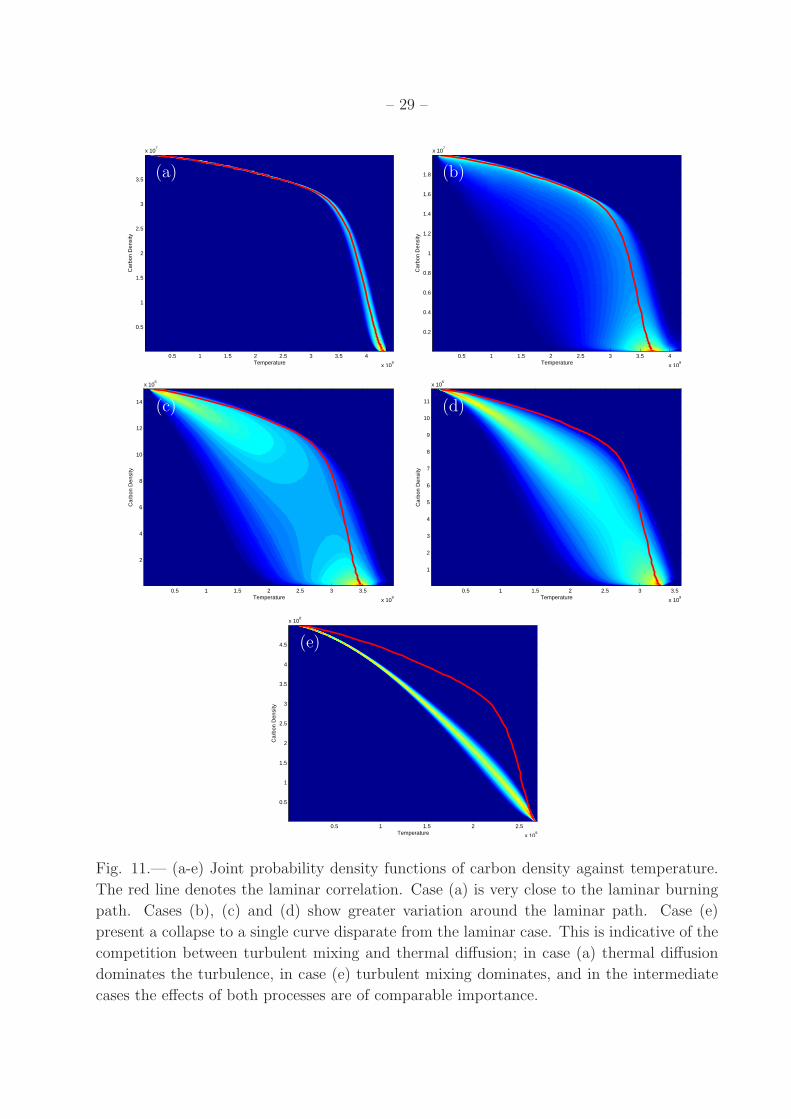
Fig. 11.— (a-e) Joint probability density functions of carbon density against temperature.

The red line denotes the laminar correlation. Case (a) is very close to the laminar burning

path. Cases (b), (c) and (d) show greater variation around the laminar path. Case (e)

present a collapse to a single curve disparate from the laminar case. This is indicative of the

competition between turbulent mixing and thermal diffusion; in case (a) thermal diffusion

dominates the turbulence, in case (e) turbulent mixing dominates, and in the intermediate

cases the effects of both processes are of comparable importance.

– 30 –

Temperature

Fue

l Con

sum

ptio

n R

ate

0.5 1 1.5 2 2.5 3 3.5 4

x 109

0.5

1

1.5

2

2.5

x 1015

(a)

Temperature

Fue

l Con

sum

ptio

n R

ate

0.5 1 1.5 2 2.5 3 3.5 4

x 109

2

4

6

8

10

12

14

x 1013

(b)

Temperature

Fue

l Con

sum

ptio

n R

ate

0.5 1 1.5 2 2.5 3 3.5

x 109

0.5

1

1.5

2

2.5

3

3.5

x 1013

(c)

Temperature

Fue

l Con

sum

ptio

n R

ate

0.5 1 1.5 2 2.5 3 3.5

x 109

0.5

1

1.5

2

2.5

3

3.5

4

4.5

5

x 1012

(d)

Temperature

Fue

l Con

sum

ptio

n R

ate

0.5 1 1.5 2 2.5

x 109

1

2

3

4

5

6

7

x 109

(e)

Fig. 12.— First moment with respect to fuel consumption rate of the joint probability density

function of fuel consumption rate against temperature. Again, the red line denotes the

laminar burning path, with which case (a) is in close agreement. Case (e) has collapsed to a

curve that is different from the laminar curve, and reiterates the lower local fuel consumption

rate observed in this case. The intermediate cases (b) through (d) show variation around the

mean path and move between the laminar and turbulent cases, and it is particularly clear

that greatly increased local fuel consumption rates are observed albeit with low probability.

– 31 –

Carbon Density

Fue

l Con

sum

ptio

n R

ate

0.05 0.1 0.15 0.2 0.25 0.3 0.35 0.4 0.45

1

2

3

4

5

6

7

x 109

Fig. 13.— First moment with respect to fuel consumption rate of the joint probability density

function of fuel consumption rate against carbon density for case (e); the other cases present

similar behavior to figures 11 and 12. This figure again shows the collapse to a burning path

different from the laminar case indicating the dominance of turbulent mixing, and the lower

local fuel consumption rates in this case, but also shows that the burning occurs at lower

carbon mass fractions than in the laminar case.

– 32 –

55 56 57 58 59 60 61 62 63 64 65

0

0.2

0.4

0.6

0.8

1

Height (cm)

Nor

mal

ised

pro

files

DensityTemperatureCarbonMagnesiumFCR

0 200 400 600 800 1000 1200

0

0.1

0.2

0.3

0.4

0.5

0.6

0.7

0.8

0.9

1

Height (cm)

Nor

mal

ised

flow

var

iabl

es

DensityTemperatureCarbonMagnesiumFCR

Fig. 14.— Comparison of laminar (left) and turbulent (right) profiles in case (e). In partic-

ular, note the disparate length scales between the two figures; the turbulent flame is around

60 times wider than the laminar flame. Each flow variable has been normalized by the min-

imum and maximum values in the laminar flame, except for the velocity which has been

normalized by the turbulent burning speed. Note the significant change in the shape of the

profiles and the relative widths. In the laminar case, thermal diffusion dominates, and so

the temperature profile (and therefore density profile) is much wider than the species mass

fraction profiles. In the turbulent case, thermal diffusion is dominated by turbulent mixing

and so the temperature, density and species mass fractions have similar profiles resembling

hyperbolic tangents. Furthermore, the fuel consumption rate is greatly reduced in the tur-

bulent case, but because of the greatly broadened flame width, the overall fuel consumption

rate is enhanced.