1

TurboPixels: Fast Superpixels Using GeometricFlows

Alex Levinshtein, Adrian Stere, Kiriakos N. Kutulakos, David J. Fleet, Sven J. DickinsonUniversity of Toronto

Toronto, Canadababalex,adrianst,kyros,fleet,sven@cs.toronto.edu

Kaleem SiddiqiMcGill UniversityMontreal, Canadasiddiqi@cim.mcgill.ca

Abstract— We describe a geometric-flow based algorithm forcomputing a dense over-segmentation of an image, often referredto as superpixels. It produces segments that on one handrespect local image boundaries, while on the other hand limitunder-segmentation through a compactness constraint. It is veryfast, with complexity that is approximately linear in imagesize, and can be applied to megapixel sized images with highsuperpixel densities in a matter of minutes. We show qualitativedemonstrations of high quality results on several complex im-ages. The Berkeley database is used to quantitatively compareits performance to a number of over-segmentation algorithms,showing that it yields less under-segmentation than algorithmsthat lack a compactness constraint, while offering a significantspeed-up over N-cuts, which does enforce compactness.

Index Terms— superpixels, image segmentation, image label-ing, perceptual grouping.

I. INTRODUCTION

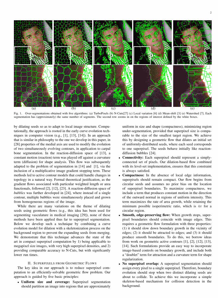
Superpixels [18] represent a restricted form of region segmenta-tion, balancing the conflicting goals of reducing image complexitythrough pixel grouping while avoiding under-segmentation. Theyhave been adopted primarily by those attempting to segment,classify or label images from labelled training data [8], [9],[10], [16], [18]. The computational cost of the underlying group-ing processes, whether probabilistic or combinatorial, is greatlyreduced by contracting the pixel graph to a superpixel graph.For many such problems, it is far easier to merge superpixelsthan to split them, implying that superpixels should aim to over-segment the image. Region segmentation algorithms which lacksome form of compactness constraint, e.g., local variation [6],mean-shift [3], or watershed [7], can lead to under-segmentationin the absence of boundary cues in the image. This can occur,for example, when there is poor contrast or shadows. Algorithmsthat do encode a compactness constraint, including N-Cuts[27]and TurboPixels (the framework we propose), offer an importantmechanism for coping with under-segmentation. Figure 1 showsthe over-segmentations obtained using these five algorithms; theeffect of a compactness constraint in limiting under-segmentationcan be clearly observed in the results produced by TurboPixelsand N-Cuts.

The superpixel algorithm of Ren and Malik [18] is a restrictedgraph cut algorithm, constrained to yield a large number of

small, compact, quasi-uniform regions. Graph cut segmentationalgorithms operate on graphs whose nodes are pixel values andwhose edges represent affinities between pixel pairs. They seeka set of recursive bi-partitions that globally minimize a costfunction based on the nodes in a segment and/or the edgesbetween segments. Wu and Leahy [26] were the first to segmentimages using graph cuts, minimizing the sum of the edge weightsacross cut boundaries. However, their algorithm is biased towardshort boundaries, leading to the creation of small regions. Tomitigate this bias, the graph cut cost can be normalized using theedge weights being cut and/or properties of the resulting regions.Although many cost functions have been proposed (e.g., [5], [11],[19], [25]), the most popular normalized cut formulation, referredto widely as N-Cuts, is due to Shi and Malik [21], and was thebasis for the original superpixel algorithm of [18].

The cost of finding globally optimal solutions is high. Sincethe normalized cut problem is NP-hard for non-planar graphs,Shi and Malik proposed a spectral approximation method with(approximate) complexity O(N3/2), where N is the numberof pixels. Space and run-time complexity also depend on thenumber of segments, and become prohibitive with large numbersof segments. In [20] a further reduction in complexity by afactor of

√N is achieved, based on a recursive coarsening of the

segmentation problem. However, the number of superpixels is nolonger directly controlled, nor is the algorithm designed to ensurethe quasi-uniformity of segment size and shape. Cour et al. [4]also proposed a linear time algorithm by solving a constrainedmulti-scale N-Cuts problem, but this complexity does not takethe number of superpixels into account. In practice, this methodremains computationally expensive and thus unsuitable for largeimages with many superpixels.

There are fast segmentation algorithms with indirect controlover the number of segments. Three examples include the localvariation graph-based algorithm of Felzenszwalb and Hutten-locher [6], the mean-shift algorithm of Comaniciu and Meer [3],and Vincent and Soille’s watershed segmentation [7]. However,as mentioned earlier, since they lack a compactness constraint,such algorithms typically produce regions of irregular shapes andsizes.

The TurboPixel algorithm introduced in this paper segments animage into a lattice-like structure of compact regions (superpixels)

2

(a) (b) (c) (d) (e)Fig. 1. Over-segmentations obtained with five algorithms: (a) TurboPixels (b) N-Cuts[27] (c) Local variation [6] (d) Mean-shift [3] (e) Watershed [7]. Eachsegmentation has (approximately) the same number of segments. The second row zooms in on the regions of interest defined by the white boxes.

by dilating seeds so as to adapt to local image structure. Compu-tationally, the approach is rooted in the early curve evolution tech-niques in computer vision (e.g., [1], [13], [14]). In an approachthat is similar in philosophy to the one we develop in this paper, in[28] properties of the medial axis are used to modify the evolutionof two simultaneously evolving contours, in application to carpalbone segmentation. In the reaction-diffusion space of [13], aconstant motion (reaction) term was played off against a curvatureterm (diffusion) for shape analysis. This flow was subsequentlyadapted to the problem of segmentation in [14] and [1], via theinclusion of a multiplicative image gradient stopping term. Thesemethods led to active contour models that could handle changes intopology in a natural way. Formal theoretical justification, as thegradient flows associated with particular weighted length or areafunctionals, followed [2], [12], [23]. A reaction-diffusion space ofbubbles was further developed in [24], where instead of a singlecontour, multiple bubbles were simultaneously placed and grownfrom homogeneous regions of the image.

While there are many variations on the theme of dilatingseeds using geometric flows (e.g., this idea has been used forsegmenting vasculature in medical imaging [29]), none of thesemethods have been applied thus far to superpixel segmentation.Below we develop such a technique by combining a curveevolution model for dilation with a skeletonization process on thebackground region to prevent the expanding seeds from merging.We demonstrate that this technique advances the state of theart in compact superpixel computation by 1) being applicable tomegapixel size images, with very high superpixel densities, and 2)providing comparable accuracy to N-Cuts, but with significantlylower run times.

II. SUPERPIXELS FROM GEOMETRIC FLOWS

The key idea in our approach is to reduce superpixel com-putation to an efficiently-solvable geometric flow problem. Ourapproach is guided by five basic principles:• Uniform size and coverage: Superpixel segmentation

should partition an image into regions that are approximately

uniform in size and shape (compactness), minimizing regionunder-segmentation, provided that superpixel size is compa-rable to the size of the smallest target region. We achievethis by designing a geometric flow that dilates an initial setof uniformly-distributed seeds, where each seed correspondsto one superpixel. The seeds behave initially like reaction-diffusion bubbles [24].

• Connectivity: Each superpixel should represent a simply-connected set of pixels. Our dilation-based flow combinedwith its level-set implementation, ensures that this constraintis always satisfied.

• Compactness: In the absence of local edge information,superpixels should remain compact. Our flow begins fromcircular seeds and assumes no prior bias on the locationof superpixel boundaries. To maximize compactness, weinclude a term that produces constant motion in the directionof the outward normal in regions of uniform intensity. Thisterm maximizes the rate of area growth, while retaining theminimum possible isoperimetric ratio, which is 4π for acircular region.

• Smooth, edge-preserving flow: When growth stops, super-pixel boundaries should coincide with image edges. Thisrequires a geometric flow formulation with three properties:(1) it should slow down boundary growth in the vicinity ofedges; (2) it should be attracted to edges; and (3) it shouldproduce smooth boundaries. To do this, we borrow ideasfrom work on geometric active contours [1], [2], [12], [13],[14]. Such formulations provide an easy way to incorporateimage-based controls on boundary growth, and include botha “doublet” term for attraction and a curvature term for shaperegularization.

• No superpixel overlap: A superpixel segmentation shouldassign every pixel to a single superpixel. Therefore, boundaryevolution should stop when two distinct dilating seeds areabout to collide. To achieve this we incorporate a simpleskeleton-based mechanism for collision detection in thebackground.

3

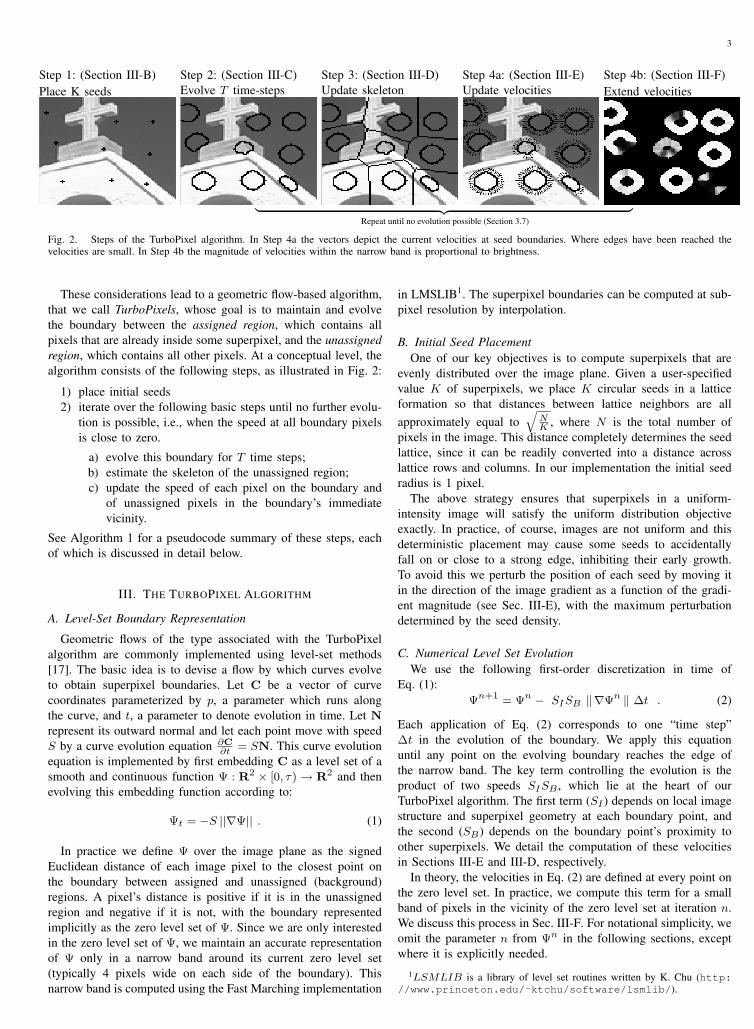
Step 1: (Section III-B) Step 2: (Section III-C) Step 3: (Section III-D) Step 4a: (Section III-E) Step 4b: (Section III-F)Place K seeds Evolve T time-steps Update skeleton Update velocities Extend velocities

︸ ︷︷ ︸Repeat until no evolution possible (Section 3.7)

Fig. 2. Steps of the TurboPixel algorithm. In Step 4a the vectors depict the current velocities at seed boundaries. Where edges have been reached thevelocities are small. In Step 4b the magnitude of velocities within the narrow band is proportional to brightness.

These considerations lead to a geometric flow-based algorithm,that we call TurboPixels, whose goal is to maintain and evolvethe boundary between the assigned region, which contains allpixels that are already inside some superpixel, and the unassignedregion, which contains all other pixels. At a conceptual level, thealgorithm consists of the following steps, as illustrated in Fig. 2:

1) place initial seeds2) iterate over the following basic steps until no further evolu-

tion is possible, i.e., when the speed at all boundary pixelsis close to zero.

a) evolve this boundary for T time steps;b) estimate the skeleton of the unassigned region;c) update the speed of each pixel on the boundary and

of unassigned pixels in the boundary’s immediatevicinity.

See Algorithm 1 for a pseudocode summary of these steps, eachof which is discussed in detail below.

III. THE TURBOPIXEL ALGORITHM

A. Level-Set Boundary Representation

Geometric flows of the type associated with the TurboPixelalgorithm are commonly implemented using level-set methods[17]. The basic idea is to devise a flow by which curves evolveto obtain superpixel boundaries. Let C be a vector of curvecoordinates parameterized by p, a parameter which runs alongthe curve, and t, a parameter to denote evolution in time. Let N

represent its outward normal and let each point move with speedS by a curve evolution equation ∂C

∂t = SN. This curve evolutionequation is implemented by first embedding C as a level set of asmooth and continuous function Ψ : R2 × [0, τ)→ R2 and thenevolving this embedding function according to:

Ψt = −S ||∇Ψ|| . (1)

In practice we define Ψ over the image plane as the signedEuclidean distance of each image pixel to the closest point onthe boundary between assigned and unassigned (background)regions. A pixel’s distance is positive if it is in the unassignedregion and negative if it is not, with the boundary representedimplicitly as the zero level set of Ψ. Since we are only interestedin the zero level set of Ψ, we maintain an accurate representationof Ψ only in a narrow band around its current zero level set(typically 4 pixels wide on each side of the boundary). Thisnarrow band is computed using the Fast Marching implementation

in LMSLIB1. The superpixel boundaries can be computed at sub-pixel resolution by interpolation.

B. Initial Seed PlacementOne of our key objectives is to compute superpixels that are

evenly distributed over the image plane. Given a user-specifiedvalue K of superpixels, we place K circular seeds in a latticeformation so that distances between lattice neighbors are allapproximately equal to

√NK , where N is the total number of

pixels in the image. This distance completely determines the seedlattice, since it can be readily converted into a distance acrosslattice rows and columns. In our implementation the initial seedradius is 1 pixel.

The above strategy ensures that superpixels in a uniform-intensity image will satisfy the uniform distribution objectiveexactly. In practice, of course, images are not uniform and thisdeterministic placement may cause some seeds to accidentallyfall on or close to a strong edge, inhibiting their early growth.To avoid this we perturb the position of each seed by moving itin the direction of the image gradient as a function of the gradi-ent magnitude (see Sec. III-E), with the maximum perturbationdetermined by the seed density.

C. Numerical Level Set EvolutionWe use the following first-order discretization in time of

Eq. (1):Ψn+1 = Ψn − SISB ‖∇Ψn ‖ ∆t . (2)

Each application of Eq. (2) corresponds to one “time step”∆t in the evolution of the boundary. We apply this equationuntil any point on the evolving boundary reaches the edge ofthe narrow band. The key term controlling the evolution is theproduct of two speeds SISB , which lie at the heart of ourTurboPixel algorithm. The first term (SI ) depends on local imagestructure and superpixel geometry at each boundary point, andthe second (SB) depends on the boundary point’s proximity toother superpixels. We detail the computation of these velocitiesin Sections III-E and III-D, respectively.

In theory, the velocities in Eq. (2) are defined at every point onthe zero level set. In practice, we compute this term for a smallband of pixels in the vicinity of the zero level set at iteration n.We discuss this process in Sec. III-F. For notational simplicity, weomit the parameter n from Ψn in the following sections, exceptwhere it is explicitly needed.

1LSMLIB is a library of level set routines written by K. Chu (http://www.princeton.edu/˜ktchu/software/lsmlib/).

4

Algorithm 1: TurboPixel AlgorithmInput: Image I, number of seeds KOutput: Superpixel boundaries BPlace K seeds on a rectangular grid in image I;1

Perturb the seed positions away from high gradient regions;2

Set all seed pixels to “assigned”;3

Set Ψ0 to be the signed Euclidean distance from the4

“assigned” regions;assigned pixels ←

∑x,y [Ψ0(x, y) >= 0];5

Compute the pixel affinity φ(x, y);6

n← 0;7

while Change in assigned pixels is large do8

Compute the image velocity SI ;9

Compute the boundary velocity SB ;10

S ← SISB ;11

Extend the speed S in a narrow band near the zero12

level-set of Ψn;Compute Ψn+1 by evolving Ψn within the narrow band;13

n← n+ 1;14

assigned pixels ←∑x,y [Ψn(x, y) >= 0];15

B ← homotopic skeleton of Ψn;16

return B17

D. Proximity-Based Boundary VelocityThe proximity-based velocity term ensures that the boundaries

of nearby superpixels never cross each other. To do this, we usea binary stopping term that is equal to 0 on the 2D homotopicskeleton of the unassigned region and is equal to 1 everywhereelse, i.e., SB(x, y) = 0 if and only if (x, y) is on the skeleton.This formulation allows the boundary of each superpixel to beguided entirely by the underlying image, until it gets very closeto another superpixel boundary.

Since the regions between evolving curves change at eachiteration of our algorithm, the skeleton must be updated as well.We do this efficiently by marking all pixels in these unassignedregions (i.e., those with Ψ(x, y) > 0) and then applying ahomotopy preserving thinning algorithm [22] on them to computethe skeleton. The thinning algorithm removes pixels ordered bytheir distance to the boundary of the region with the constraintthat all digital points that can be removed without altering thetopology are removed.

E. Image-Based Boundary VelocityOur image-based speed term combines the reaction-diffusion

based shape segmentation model of [1], [14], [24] with anadditional “doublet” term provided by the geodesic active contour[2], [12] to attract the flow to edges:

SI(x, y) = [ 1− ακ(x, y) ]φ(x, y)︸ ︷︷ ︸reaction-diffusion term

−β [ N(x, y) · ∇φ(x, y) ]︸ ︷︷ ︸“doublet” term

.

(3)The reaction-diffusion term ensures that the boundary’s evolu-

tion slows down when it gets close to a high-gradient region inthe image. It is controlled by three quantities: (1) a “local affinity”function φ(x, y), computed for every pixel on the image plane,that is low near edges and high elsewhere; (2) a curvature functionκ(x, y) that expresses the curvature of the boundary at point(x, y) and smoothes the evolving boundary; and (3) a “balancing”parameter α that weighs the contribution of the curvature term.

Intuitively, the doublet term ensures that the boundary isattracted to image edges, i.e., pixels where the affinity is low.Specifically, when a point (x, y) on the boundary evolves towarda region of decreasing affinity (an image edge), its normalN(x, y) will coincide with the negative gradient direction of φ,and the term acts as an attractive force. If the boundary crossesover an edge these two vectors will point in the same directionand cause a reversal in the boundary’s direction of motion.

Local affinity function Our algorithm does not depend on aspecific definition of the function φ, as long as it is low on edgesand is high elsewhere. For almost all the experiments in this paper,we used a simple affinity measure based on the grayscale intensitygradient:

φ(x, y) = e−E(x,y)/ν , E(x, y) =‖∇I‖

Gσ∗‖∇I‖+ γ. (4)

Our affinity function φ produces high velocities in areas withlow gradients, with an upper bound of 1. Dividing the gradientmagnitude in E(x, y) by a local weighted sum of gradientmagnitudes provides a simple form of contrast normalization.The support width of the normalization, controlled by σ, isproportional to the expected initial distance between seeds. Thisnormalization allows weak but isolated edges to have a significanteffect on speed, while suppressing edge strength in dense texture.The constant γ ensures that the effect of insignificant signalgradients remains small. We note that whereas our E(x, y) is asimple measure of grayscale image gradient, the implementationof N-Cuts we use for comparison ([27]) in our experiments inSection IV employs a more complex measure of interveningcontours computed using a texture-based edge map.

Normal and curvature functions The outward normal of thezero level set of Ψ at a point (x, y) is given by the derivatives ofΨ, i.e., N = ∇Ψ/‖∇Ψ ‖. The curvature of the zero level set, ata point (x, y), is given by [17]:

κ =ΨxxΨ2

y − 2ΨxΨyΨxy + ΨyyΨ2x

(Ψ2x + Ψ2

y)32

. (5)

As is standard for diffusive terms, the derivatives of Ψ used forκ are computed using central difference approximations. Centraldifference approximations are also used for all other calculationswith the exception of ‖∇Ψn ‖ in the level set form for thereaction term (φ(x, y)) in Eq. 3, for which upwind derivatives[17] must be used since it is a hyperbolic term.

Balancing parameters The balancing parameters α and β inEq. 3 control the relative contributions of the reaction-diffusionand doublet terms. Higher values of α prevent “leakage” throughnarrow edge gaps, but also prevent sharp superpixel boundariesthat may be sometimes desirable. High values of β cause betterstopping behavior of seeds on weak edges, but also slow downthe evolution of seeds elsewhere.2

F. Speed ExtensionThe velocity terms SI and SB have meaning only on the current

superpixel boundaries, i.e., the zero level set of Ψ. This leads

2Based on empirical observation, the values α = 0.3 and β = 1 werechosen. These values limit the amount of leakage during seed evolution,without slowing down the evolution in other regions. In the future, we intendto learn the optimal values for these parameters automatically by evaluatingthe performance of the algorithm on a training set of images.

5

to two technical difficulties. First, the zero level set is definedimplicitly and, hence, it lies “in between” the discrete imagepixels. Second, each time we invoke a level set update iteration(Eq. 2), the boundary must move by a finite amount (i.e., at leasta sizeable fraction of a pixel).

Speed extension gives a way to solve both problems and iscommon in existing curve evolution implementations [14]. Here,we extend φ and ∇φ, the only image-dependent terms, in thesame narrow band we use to maintain an accurate estimate ofΨ (see Sec. III-C). To each pixel (x, y) in this narrow band, wesimply assign the φ and ∇φ values of its closest pixel on theboundary3.

G. Termination Conditions & Final SegmentationThe algorithm terminates when the boundaries stop evolving.

Since in theory the boundaries can evolve indefinitely with ever-decreasing velocities, the algorithm terminates when the relativeincrease of the total area covered by superpixels falls below athreshold. We used a relative area threshold of 10−4 in all ourexperiments.

After termination, the evolution results are post-processed sothat the superpixel boundaries are exactly one pixel in width.This is done in three steps. First, any remaining large unas-signed connected regions are treated as superpixels. Next, verysmall superpixels are removed, making their corresponding pixelsunassigned. Finally, these unassigned regions are thinned, as inSec. III-D, according to the algorithm in [22]. The thinning isordered by a combination of Euclidean distance to the boundaryand a φ-based term, in order to obtain smooth superpixel contoursthat are close to edges.

H. Algorithm ComplexityThe complexity of our algorithm is roughly linear in the total

number of image pixels N for a fixed superpixel density. At eachtime step, all elements of the distance function Ψ are updated(see Eq. 2). Each update requires the computation of the partialderivatives of Ψ and evaluation of SISB . Thus each update takesO(N) operations.

The speed extension and homotopic skeleton computations arenot linear in image size. Both actions are O(N logN) but can bemade faster in practice. If b is the number of pixels in the narrowband (which is linear in the number of pixels that lie on zero-crossings), then the complexity of speed extension is O(N) +

O(b log b). While b can approach N in theory, it is usually muchsmaller in practice.

The homotopic skeleton computation isO(N)+O(k log k) [22],where k is the number of unassigned pixels. In practice, k � N ,especially toward the end of the evolution when few unassignedpixels remain.

It now remains to take into account the number of iterationsof the algorithm. Under ideal conditions, all the curves evolvewith maximal speed until they meet or reach an edge. Since theexpected distance between seeds is Dn initially (see Sec. III-B), it will take O(

√NK ) iterations for the algorithm to converge.

Hence, the algorithm converges more slowly for larger images,and more quickly as the superpixel density increases. Thus fora fixed superpixel density (keeping Dn constant), the number of

3The algorithm that efficiently computes Ψ for all pixels within the narrowband provides their closest boundary pixel as a byproduct, so no extracomputations are necessary.

100 150 200 250 300 350 400 450 500 5500

0.05

0.1

0.15

0.2

0.25

0.3

0.35

Number of superpixels

Und

erse

gmen

tatio

n E

rror

Turbo

Felz

SB

Ncuts

100 150 200 250 300 350 400 450 500 5500.55

0.6

0.65

0.7

0.75

0.8

0.85

0.9

0.95

1

Number of superpixels

Bou

ndar

y re

call

Turbo

Felz

SB

Ncuts

(a) (b)Fig. 3. Under-segmentation error (a) and accuracy (boundary recall) (b) asa function of superpixel density.

iterations will be constant, making the overall complexity roughlyO(N).

IV. EXPERIMENTAL RESULTS

We evaluate the performance of the TurboPixel algorithm bycomparing its accuracy and running time to three other algo-rithms: Normalized Cuts (Ncuts) and square blocks (Sb), bothof which encode a compactness constraint, and Felzenszwalb andHuttenlocher (Felz), which does not. The TurboPixel algorithmwas implemented in Matlab with several C extensions4. ForNcuts, we use the 2004 Ncut implementation based on [27]5,while for Sb, we simply divide the image into even rectangularblocks, providing a naive but efficient benchmark for accuracy(other algorithms are expected to do better). All experiments wereperformed on a quad-core Xeon 3.6 Ghz computer. We use theBerkeley database, which contains 300 (481×321 or 321×481)images. In our experiments, the image size is defined as thefraction of the area of the full image size of 154401 pixels. Inall experiments, performance/accuracy is averaged over at least25 images and in most cases over a larger number.6 Finally, thegradient-based affinity function of a grayscale image (Eq. 4) wasused for the TurboPixel algorithm, a difference in image intensitywas used as affinity in Felz, and a more elaborate (interveningcontours) affinity was used for Ncuts.

A. Under-segmentation Error

As stated in Section I, algorithms that do not enforce a com-pactness constraint risk a greater degree of under-segmentation.Given a ground-truth segmentation into segments g1, . . . , gKand a superpixel segmentation into superpixels s1, . . . , sL, wequantify the under-segmentation error for segment gi with thefraction [∑

{sj | sj∩gi 6=∅}Area(sj)]− Area(gi)

Area(gi). (6)

Intuitively, this fraction measures the total amount of “bleeding”caused by superpixels that overlap a given ground-truth segment,normalized by the segment’s area.

To evaluate the under-segmentation performance of a givenalgorithm, we simply average the above fraction across allground-truth segments and all images. Figure 3(a) compares

4A beta-version of our code is available at http://www.cs.toronto.edu/˜babalex/turbopixels_supplementary.tar.gz; the de-fault parameter values are the same as those used for the experiments inthis article.

5We use Version 7 from Jianbo Shi’s website http://www.cis.upenn.edu/˜jshi/software/files/NcutImage_7_1.zip

6Due to the long running time and large memory requirements of Ncuts,using the entire database was prohibitively expensive.

6

0.2 0.3 0.4 0.5 0.6 0.7 0.8 0.9 10

5

10

15

20

25

30

35

40

Image size (normalized # of pixels)

Tim

e (m

in)

TurboPixelsN−Cuts

0.2 0.3 0.4 0.5 0.6 0.7 0.8 0.9 10

5

10

15

20

25

30

Image size (normalized # of pixels)

Tim

e (s

ec)

1 2 3 4 50

5

10

15

20

25

Number of superpixels (100s)

Tim

e (m

in)

TurboPixelsN−Cuts

1 2 3 4 50

1

2

3

4

5

6

7

Number of superpixels (100s)

Tim

e (s

ec)

(a) (b) (c) (d)

Fig. 4. Timing evaluation. (a) Running time vs. image size. (b) An expanded version (a) to show the behavior of the TurboPixel algorithm. (c) Runningtime vs. superpixel density. (d) An expanded version of (c) showing the behavior of the TurboPixel algorithm.

the four algorithms using this metric, with under-segmentationerror plotted as a function of superpixel density. The inability ofFelz to stem the bleeding is reflected in the significantly higherunder-segmentation error over all three algorithms that encode acompactness constraint. Of these three, the TurboPixel algorithmachieves the least under-segmentation error.

B. Boundary Recall

Since precise boundary shape might be necessary for some ap-plications, we adopt a standard measure of boundary recall (whatfraction of the ground truth edges fall within a small distancethreshold (2 pixels in this experiment) from at least 1 superpixelboundary. As shown in Fig. 3(b), Felz offers better recall at lowersuperpixel densities, while at higher superpixel densities, Felz andTurboPixel are comparable, with both outperforming Ncuts andSb. The fact that Felz does not constrain its superpixels to becompact means that it can better capture the boundaries of thin,non-compact regions at lower superpixel densities.

C. Timing Evaluation

With the exception of the naive and clearly inferior Sb algo-rithm, the cost of enforcing a compactness constraint (Ncuts,TurboPixel) is significant; for example, Felz is, on average,10 times faster than TurboPixel. For our timing analysis, wetherefore restrict our comparison to TurboPixel and Ncuts, the twoprimary competitors in the class of algorithms with a compactnessconstraint. For any superpixel algorithm, it is appropriate toincrease the number of superpixels as the image size increases,so that the expected area (in pixels) of each superpixel remainsconstant. Fig. 4 (a and b) shows the running time of the twoalgorithms as a function of increased image size. The expectedsize of a superpixel is kept fixed at about 10×10 pixels.

The TurboPixel algorithm is several orders of magnitude faster.It is almost linear in image size compared to Ncuts, whose runningtime increases non-linearly. Due to “out of memory” errors, wewere unable to run Ncuts for all of the parameter settings usedfor the TurboPixel results. Fig. 4 (c and d) show running timeas a function of superpixel density, with the image size fixedat 240×160 (one quarter of the original size). The running timeof Ncuts increases in a non-linear fashion whereas the runningtime of the TurboPixel algorithm decreases as the density of thesuperpixels increases. This is due to the fact that the seeds evolveover a smaller spatial extent on average and thus converge faster.

D. Qualitative Results

Fig. 5 gives a qualitative feel for the superpixels obtainedby the TurboPixel algorithm for a variety of images from the

Berkeley database. Observe that the superpixel boundaries respectthe salient edges in each image, while remaining compact and uni-form in size.7 Fig. 6 provides a qualitative comparison against theresults obtained using Ncuts. The TurboPixel algorithm obtainssuperpixels that are more regularly shaped and uniform in sizethan those of Ncuts.

The TurboPixel algorithm is of course not restricted to workwith affinity functions that are based strictly on image gradient,as discussed in Section III-E, and hence more refined measurescan be used for superpixel boundary velocity. Fig. 7 showsthe performance of the algorithm when the boundary velocityincorporates the Pb edge detector [15]. Note how the edgebetween the leopard and the background is captured much betterwhen a Pb-based affinity is used. Moreover, the shapes of thesuperpixels inside the leopard are more regular for the latter case.

V. CONCLUSIONS

The task of efficiently computing a highly regular over-segmentation of an image can be effectively formulated as a set oflocally interacting region growing problems, and as such avoidsthe high cost of computing globally optimal over-segmentations(or their approximations), such as N-Cuts. Combining the powerof a data-driven curve evolution process with a set of skeletal-based external constraints represents a novel, highly efficientframework for superpixel segmentation. The results clearly indi-cate that while superpixel quality is comparable to the benchmarkalgorithm, our algorithm is several orders of magnitude faster,allowing it to be applied to large megapixel images with verylarge superpixel densities.

The framework is general and, like any region segmentationalgorithm, is based on a user-defined measure of affinity betweenpixels. While our experiments have demonstrated the use ofintensity gradient-based and Pb-based affinities, other more com-plex affinity measures, perhaps incorporating information frommultiple scales, are possible. Selecting the appropriate affinitymeasure is entirely task dependent. We offer no prescription, butrather offer a general framework into which a domain-dependentaffinity measure can be incorporated.

It is also important to note that we have intentionally skirtedseveral important domain-dependent problems. One global issueis the fact that our framework allows the user to control thesuperpixel shape and density. On the issue of density, our ap-proach is very generic, and one could imagine that with domain

7Supplementary material (http://www.cs.toronto.edu/˜babalex/turbopixels_supplementary.tar.gz) containsadditional results of the TurboPixel algorithm on megapixel sized imageswith superpixel densities in the thousands. Obtaining superpixels under suchconditions using Ncuts is prohibitively expensive.

7

Fig. 5. TurboPixel results on a variety of images from the Berkeley database, with a zoom-in on selected regions in the middle and right columns.

Ncuts TurboPixels Ncuts TurboPixelsFig. 6. A qualitative comparison of TurboPixel results with gray-level gradient-based affinity compared to results with Ncuts.

knowledge, seeds could be placed much more judiciously. Anddepending on the task, seeds could be placed with varying densityat the cost of lower superpixel uniformity. In some domains,varying seed density may be more desirable. In textured images,for example, seeds could be placed to capture the individualtexture elements better (like the spots of the leopard in Figure 6).Moreover, our framework allows us to guide superpixels to have acertain shape. Currently, in the absence of edges, the superpixelswould grow in a circular manner. However, one could imagine

growing superpixels to be elliptical instead. This could be moreuseful for extracting superpixels in narrow structures. Still, asshown in the experiments, the use of a compactness constraintclearly minimizes under-segmentation at a significantly highercomputational cost. If both under-segmentation and irregularlyshaped superpixel boundaries can be tolerated, the Felz algorithmis clearly the better choice, offering a tenfold speed-up as well asimproved boundary recall at lower superpixel densities.

Perhaps the most important issue is what to do with the

8

Fig. 7. Qualitative results of the TurboPixel algorithm using gradient-based (middle) and Pb-based (right) affinity functions.

(a) (b)

(c) (d)Fig. 8. Image representation using superpixels. Each superpixel from the original image (a) is colored with: (b) The average color of the original pixels init. (c) The best linear fit to the color of the original pixels in it. (d) The best quadratic fit to the color of the original pixels in it.

resulting superpixels. The application possibilities are numerous,ranging from image compression to perceptual grouping to figure-ground segmentation. Currently, superpixels are mainly used forimage labeling problems to avoid the complexity of having tolabel many more pixels. In the same manner, superpixels canbe used as the basis for image segmentation. In the graphcuts segmentation algorithm, the affinity can be defined oversuperpixels instead of over pixels, resulting in a much smallergraph. Superpixels can also be considered as a compact imagerepresentation. To illustrate this idea, in Figure 8 each superpixel’scolor is approximated by three polynomials (one per channel).Note that whereas the mean and the linear approximations seempoor, the quadratic approximation approaches the quality of theoriginal image.

ACKNOWLEDGMENTS

We thank Timothee Cour and Jianbo Shi for making their N-Cut package available, and Kevin Chu for his level set methodlibrary (LSMLIB), used in our TurboPixel implementation.

REFERENCES

[1] V. Caselles, F. Catte, T. Coll, and F. Dibos. A geometric model foractive contours in image processing. Num. Mathematik, 66:1–31, 1993.

[2] V. Caselles, R. Kimmel, and G. Sapiro. Geodesic active contours. IEEEICCV, pp. 694–699, 1995.

[3] D. Comaniciu and P. Meer. Mean shift: A robust approach toward featurespace analysis. IEEE Trans. PAMI, 24(5):603–619, 2002.

[4] T. Cour, F. Benezit, and J. Shi. Spectral segmentation with multiscalegraph decomposition. IEEE CVPR, vol. 2, pp. 1124–1131, 2005.

[5] I. Cox, S. Rao, and Y. Zhong. ’ratio regions’: A technique for imagesegmentation. ICPR, pp. B:557–564, 1996.

9

[6] P. Felzenszwalb and D. Huttenlocher. Efficient graph-based imagesegmentation. IJCV, 59(2):167–181, 2004.

[7] Luc Vincent and Pierre Soille. Watersheds in Digital Spaces: AnEfficient Algorithm Based on Immersion Simulations. PAMI, 13(6):583–598, 1991.

[8] X. He, R. Zemel, and D. Ray. Learning and incorporating top-downcues in image segmentation. ECCV, vol. 1, pp. 338–351, 2006.

[9] D. Hoiem, A. Efros, and M. Hebert. Automatic photo pop-up. ACMTrans. Graph., 24(3):577–584, 2005.

[10] D. Hoiem, A. Efros, and M. Hebert. Geometric context from a singleimage. IEEE ICCV, pp. 654–661, 2005.

[11] I. Jermyn and H. Ishikawa. Globally optimal regions and boundaries asminimum ratio weight cycles. IEEE Trans. PAMI, 23(10):1075–1088,2001.

[12] S. Kichenassamy, A. Kumar, P. Olver, A. Tannenbaum, and A. Yezzi.Gradient flows and geometric active contour models. IEEE ICCV, pp.810–815, 1995.

[13] B. Kimia, A. Tannenbaum, and S. Zucker. Toward a computationaltheory of shape: An overview. Lecture Notes in Computer Science,427:402–407, 1990.

[14] R. Malladi, J. Sethian, and B. Vemuri. Shape modeling with frontpropagation: A level set approach. IEEE Trans. PAMI, 17(2):158–175,1995.

[15] D. Martin, C. Fowlkes, and J. Malik. Learning to detect natural imageboundaries using local brightness, color, and texture cues. IEEE TransPAMI 26(5):530–549, 2004.

[16] G. Mori, X. Ren, A. Efros, and J. Malik. Recovering human bodyconfigurations: Combining segmentation and recognition. IEEE CVPR,vol. 2, pp. 326–333, 2004.

[17] S. Osher and J. Sethian. Fronts propagation with curvature dependentspeed: Algorithms based on hamilton-jacobi formulations. J. Comp.Physics, 79:12–49, 1988.

[18] X. Ren and J. Malik. Learning a classification model for segmentation.IEEE ICCV, pp. 10–17, 2003.

[19] S. Sarkar and P. Soundararajan. Supervised learning of large perceptualorganization: Graph spectral partitioning and learning automata. IEEEPAMI, 22:504–525, 2000.

[20] E. Sharon, A. Brandt, and R. Basri. Fast multiscale image segmentation.IEEE CVPR, vol. 1, pp. 70–77 2000.

[21] J. Shi and J. Malik. Normalized cuts and image segmentation. IEEETrans. PAMI, 22(8):888–905, 2000.

[22] K. Siddiqi, S. Bouix, A. Tannenbaum, and S. Zucker. Hamilton-jacobiskeletons. IJCV, 48(3):215–231, 2002.

[23] K. Siddiqi, Y. Lauziere, A. Tannenbaum, and S. Zucker. Area and lengthminimizing flows for shape segmentation. IEEE Trans. IP, 7(3):433–443, 1998.

[24] H. Tek and B. Kimia. Image Segmentation by Reaction-DiffusionBubbles. IEEE ICCV, pp. 156–162, 1995.

[25] S. Wang and M. Siskind. Image segmentation with ratio cut - supple-mental material. IEEE Trans. PAMI, 25(6):675–690, 2003.

[26] Z. Wu and R. Leahy. An optimal graph theoretic approach to dataclustering: Theory and application to image segmentation. IEEE Trans.PAMI, 15(11):1101–1113, 1993.

[27] S. Yu and J. Shi. Multiclass spectral clustering. IEEE ICCV, vol. 1, pp.313–319, 2003.

[28] Thomas B. Sebastian, Huseyin Tek, Joseph J. Crisco, Scott W. Wolfe,and Benjamin B. Kimia. Segmentation of Carpal Bones from 3d CTImages Using Skeletally Coupled Deformable Models. MICCAI, pp.1184–1194, 1998.

[29] L. Lorigo, O. Faugeras, W. Grimson, R. Keriven, R. Kikinis, A. Nabavi,and C. Westin. Codimension-Two Geodesic Active Contours for theSegmentation of Tubular Structures. CVPR, pp. 444–451, 2000.