Embed Size (px)
Citation preview

ibm.com/redbooks Redpaper
Front cover
Tuning Red Hat Enterprise Linux on IBM Eserver xSeries Servers
Eduardo Ciliendo
Describes ways to tune the operating system
Introduces performance tuning tools
Covers key server applications


International Technical Support Organization
Tuning Red Hat Enterprise Linux on IBM Eserver xSeries Servers
July 2005

© Copyright International Business Machines Corporation 2005. All rights reserved.Note to U.S. Government Users Restricted Rights -- Use, duplication or disclosure restricted by GSA ADP ScheduleContract with IBM Corp.
Second Edition (July 2005)
This edition applies to Red Hat Enterprise Linux AS running on IBM Eserver xSeries servers.
Note: Before using this information and the product it supports, read the information in “Notices” on page vii.

© Copyright IBM Corp. 2005. All rights reserved. iii
Contents
Notices . . . . . . . . . . . . . . . . . . . . . . . . . . . . . . . . . . . . . . . . . . . . . . . . . . . . . . . . . . . . . . . . . viiTrademarks . . . . . . . . . . . . . . . . . . . . . . . . . . . . . . . . . . . . . . . . . . . . . . . . . . . . . . . . . . . . . viii
Preface . . . . . . . . . . . . . . . . . . . . . . . . . . . . . . . . . . . . . . . . . . . . . . . . . . . . . . . . . . . . . . . . . ixHow this Redpaper is structured . . . . . . . . . . . . . . . . . . . . . . . . . . . . . . . . . . . . . . . . . . . . . . ixThe team that wrote this Redpaper . . . . . . . . . . . . . . . . . . . . . . . . . . . . . . . . . . . . . . . . . . . . .xBecome a published author . . . . . . . . . . . . . . . . . . . . . . . . . . . . . . . . . . . . . . . . . . . . . . . . . . xiComments welcome. . . . . . . . . . . . . . . . . . . . . . . . . . . . . . . . . . . . . . . . . . . . . . . . . . . . . . . . xi
Chapter 1. Understanding Linux performance . . . . . . . . . . . . . . . . . . . . . . . . . . . . . . . . . 11.1 The Linux CPU scheduler . . . . . . . . . . . . . . . . . . . . . . . . . . . . . . . . . . . . . . . . . . . . . . . . 31.2 The Linux memory architecture. . . . . . . . . . . . . . . . . . . . . . . . . . . . . . . . . . . . . . . . . . . . 41.3 The virtual memory manager . . . . . . . . . . . . . . . . . . . . . . . . . . . . . . . . . . . . . . . . . . . . . 51.4 Modular I/O elevators . . . . . . . . . . . . . . . . . . . . . . . . . . . . . . . . . . . . . . . . . . . . . . . . . . . 6
1.4.1 Anticipatory . . . . . . . . . . . . . . . . . . . . . . . . . . . . . . . . . . . . . . . . . . . . . . . . . . . . . . . 71.4.2 Complete Fair Queuing (CFQ) . . . . . . . . . . . . . . . . . . . . . . . . . . . . . . . . . . . . . . . . 71.4.3 Deadline . . . . . . . . . . . . . . . . . . . . . . . . . . . . . . . . . . . . . . . . . . . . . . . . . . . . . . . . . 71.4.4 NOOP . . . . . . . . . . . . . . . . . . . . . . . . . . . . . . . . . . . . . . . . . . . . . . . . . . . . . . . . . . . 7
1.5 The network subsystem . . . . . . . . . . . . . . . . . . . . . . . . . . . . . . . . . . . . . . . . . . . . . . . . . 71.5.1 TCP/IP transfer window . . . . . . . . . . . . . . . . . . . . . . . . . . . . . . . . . . . . . . . . . . . . . 8
1.6 Linux file systems . . . . . . . . . . . . . . . . . . . . . . . . . . . . . . . . . . . . . . . . . . . . . . . . . . . . . . 91.6.1 ext2 . . . . . . . . . . . . . . . . . . . . . . . . . . . . . . . . . . . . . . . . . . . . . . . . . . . . . . . . . . . . . 91.6.2 ext3, the default Red Hat file system . . . . . . . . . . . . . . . . . . . . . . . . . . . . . . . . . . . 91.6.3 ReiserFS . . . . . . . . . . . . . . . . . . . . . . . . . . . . . . . . . . . . . . . . . . . . . . . . . . . . . . . . . 91.6.4 JFS . . . . . . . . . . . . . . . . . . . . . . . . . . . . . . . . . . . . . . . . . . . . . . . . . . . . . . . . . . . . 101.6.5 XFS . . . . . . . . . . . . . . . . . . . . . . . . . . . . . . . . . . . . . . . . . . . . . . . . . . . . . . . . . . . . 10
1.7 The proc file system . . . . . . . . . . . . . . . . . . . . . . . . . . . . . . . . . . . . . . . . . . . . . . . . . . . 101.8 Understanding Linux performance metrics . . . . . . . . . . . . . . . . . . . . . . . . . . . . . . . . . . 12
1.8.1 Processor metrics . . . . . . . . . . . . . . . . . . . . . . . . . . . . . . . . . . . . . . . . . . . . . . . . . 121.8.2 Memory metrics. . . . . . . . . . . . . . . . . . . . . . . . . . . . . . . . . . . . . . . . . . . . . . . . . . . 131.8.3 Network interface metrics . . . . . . . . . . . . . . . . . . . . . . . . . . . . . . . . . . . . . . . . . . . 131.8.4 Block device metrics . . . . . . . . . . . . . . . . . . . . . . . . . . . . . . . . . . . . . . . . . . . . . . . 14
Chapter 2. Monitoring tools . . . . . . . . . . . . . . . . . . . . . . . . . . . . . . . . . . . . . . . . . . . . . . . 152.1 Overview of tool function. . . . . . . . . . . . . . . . . . . . . . . . . . . . . . . . . . . . . . . . . . . . . . . . 162.2 uptime . . . . . . . . . . . . . . . . . . . . . . . . . . . . . . . . . . . . . . . . . . . . . . . . . . . . . . . . . . . . . . 162.3 dmesg . . . . . . . . . . . . . . . . . . . . . . . . . . . . . . . . . . . . . . . . . . . . . . . . . . . . . . . . . . . . . . 172.4 top . . . . . . . . . . . . . . . . . . . . . . . . . . . . . . . . . . . . . . . . . . . . . . . . . . . . . . . . . . . . . . . . . 18
2.4.1 Process priority and nice levels. . . . . . . . . . . . . . . . . . . . . . . . . . . . . . . . . . . . . . . 192.4.2 Zombie processes. . . . . . . . . . . . . . . . . . . . . . . . . . . . . . . . . . . . . . . . . . . . . . . . . 19
2.5 iostat . . . . . . . . . . . . . . . . . . . . . . . . . . . . . . . . . . . . . . . . . . . . . . . . . . . . . . . . . . . . . . . 202.6 vmstat . . . . . . . . . . . . . . . . . . . . . . . . . . . . . . . . . . . . . . . . . . . . . . . . . . . . . . . . . . . . . . 212.7 ps and pstree . . . . . . . . . . . . . . . . . . . . . . . . . . . . . . . . . . . . . . . . . . . . . . . . . . . . . . . . 222.8 numastat . . . . . . . . . . . . . . . . . . . . . . . . . . . . . . . . . . . . . . . . . . . . . . . . . . . . . . . . . . . . 222.9 sar . . . . . . . . . . . . . . . . . . . . . . . . . . . . . . . . . . . . . . . . . . . . . . . . . . . . . . . . . . . . . . . . . 232.10 KDE System Guard. . . . . . . . . . . . . . . . . . . . . . . . . . . . . . . . . . . . . . . . . . . . . . . . . . . 24
2.10.1 Work space . . . . . . . . . . . . . . . . . . . . . . . . . . . . . . . . . . . . . . . . . . . . . . . . . . . . . 252.11 Gnome System Monitor . . . . . . . . . . . . . . . . . . . . . . . . . . . . . . . . . . . . . . . . . . . . . . . 282.12 free . . . . . . . . . . . . . . . . . . . . . . . . . . . . . . . . . . . . . . . . . . . . . . . . . . . . . . . . . . . . . . . 28

iv Tuning Red Hat Enterprise Linux on IBM Eserver xSeries Servers
2.13 pmap . . . . . . . . . . . . . . . . . . . . . . . . . . . . . . . . . . . . . . . . . . . . . . . . . . . . . . . . . . . . . . 292.14 strace . . . . . . . . . . . . . . . . . . . . . . . . . . . . . . . . . . . . . . . . . . . . . . . . . . . . . . . . . . . . . 292.15 ulimit . . . . . . . . . . . . . . . . . . . . . . . . . . . . . . . . . . . . . . . . . . . . . . . . . . . . . . . . . . . . . . 302.16 mpstat . . . . . . . . . . . . . . . . . . . . . . . . . . . . . . . . . . . . . . . . . . . . . . . . . . . . . . . . . . . . . 312.17 Capacity Manager . . . . . . . . . . . . . . . . . . . . . . . . . . . . . . . . . . . . . . . . . . . . . . . . . . . . 32
Chapter 3. Tuning the operating system . . . . . . . . . . . . . . . . . . . . . . . . . . . . . . . . . . . . . 353.1 Change management . . . . . . . . . . . . . . . . . . . . . . . . . . . . . . . . . . . . . . . . . . . . . . . . . . 363.2 Installation . . . . . . . . . . . . . . . . . . . . . . . . . . . . . . . . . . . . . . . . . . . . . . . . . . . . . . . . . . . 363.3 Daemons. . . . . . . . . . . . . . . . . . . . . . . . . . . . . . . . . . . . . . . . . . . . . . . . . . . . . . . . . . . . 383.4 Changing run levels . . . . . . . . . . . . . . . . . . . . . . . . . . . . . . . . . . . . . . . . . . . . . . . . . . . 403.5 Limiting local terminals . . . . . . . . . . . . . . . . . . . . . . . . . . . . . . . . . . . . . . . . . . . . . . . . . 423.6 SELinux. . . . . . . . . . . . . . . . . . . . . . . . . . . . . . . . . . . . . . . . . . . . . . . . . . . . . . . . . . . . . 423.7 Compiling the kernel . . . . . . . . . . . . . . . . . . . . . . . . . . . . . . . . . . . . . . . . . . . . . . . . . . . 433.8 Changing kernel parameters. . . . . . . . . . . . . . . . . . . . . . . . . . . . . . . . . . . . . . . . . . . . . 44
3.8.1 Where the parameters are stored . . . . . . . . . . . . . . . . . . . . . . . . . . . . . . . . . . . . . 453.8.2 Using the sysctl command . . . . . . . . . . . . . . . . . . . . . . . . . . . . . . . . . . . . . . . . . . 46
3.9 Kernel parameters. . . . . . . . . . . . . . . . . . . . . . . . . . . . . . . . . . . . . . . . . . . . . . . . . . . . . 463.10 Tuning the processor subsystem . . . . . . . . . . . . . . . . . . . . . . . . . . . . . . . . . . . . . . . . 47
3.10.1 Selecting the correct kernel . . . . . . . . . . . . . . . . . . . . . . . . . . . . . . . . . . . . . . . . 493.10.2 Interrupt handling . . . . . . . . . . . . . . . . . . . . . . . . . . . . . . . . . . . . . . . . . . . . . . . . 493.10.3 Considerations for NUMA systems . . . . . . . . . . . . . . . . . . . . . . . . . . . . . . . . . . . 49
3.11 Tuning the memory subsystem . . . . . . . . . . . . . . . . . . . . . . . . . . . . . . . . . . . . . . . . . . 503.11.1 Configuring bdflush (kernel 2.4 only) . . . . . . . . . . . . . . . . . . . . . . . . . . . . . . . . . 503.11.2 Configuring kswapd (kernel 2.4 only) . . . . . . . . . . . . . . . . . . . . . . . . . . . . . . . . . 513.11.3 Setting kernel swap behavior (kernel 2.6 only) . . . . . . . . . . . . . . . . . . . . . . . . . . 513.11.4 HugeTLBfs . . . . . . . . . . . . . . . . . . . . . . . . . . . . . . . . . . . . . . . . . . . . . . . . . . . . . 52
3.12 Tuning the file system . . . . . . . . . . . . . . . . . . . . . . . . . . . . . . . . . . . . . . . . . . . . . . . . . 523.12.1 Hardware considerations before installing Linux. . . . . . . . . . . . . . . . . . . . . . . . . 523.12.2 Other journaling file systems. . . . . . . . . . . . . . . . . . . . . . . . . . . . . . . . . . . . . . . . 553.12.3 File system tuning . . . . . . . . . . . . . . . . . . . . . . . . . . . . . . . . . . . . . . . . . . . . . . . . 55
3.13 The swap partition. . . . . . . . . . . . . . . . . . . . . . . . . . . . . . . . . . . . . . . . . . . . . . . . . . . . 603.14 Tuning the network subsystem . . . . . . . . . . . . . . . . . . . . . . . . . . . . . . . . . . . . . . . . . . 61
3.14.1 Speed and duplexing . . . . . . . . . . . . . . . . . . . . . . . . . . . . . . . . . . . . . . . . . . . . . 613.14.2 MTU size. . . . . . . . . . . . . . . . . . . . . . . . . . . . . . . . . . . . . . . . . . . . . . . . . . . . . . . 613.14.3 Increasing network buffers . . . . . . . . . . . . . . . . . . . . . . . . . . . . . . . . . . . . . . . . . 623.14.4 Increasing the packet queues . . . . . . . . . . . . . . . . . . . . . . . . . . . . . . . . . . . . . . . 623.14.5 Window sizes and window scaling . . . . . . . . . . . . . . . . . . . . . . . . . . . . . . . . . . . 623.14.6 Increasing the transmit queue length . . . . . . . . . . . . . . . . . . . . . . . . . . . . . . . . . 633.14.7 Decreasing interrupts . . . . . . . . . . . . . . . . . . . . . . . . . . . . . . . . . . . . . . . . . . . . . 633.14.8 Advanced networking options . . . . . . . . . . . . . . . . . . . . . . . . . . . . . . . . . . . . . . . 64
3.15 Driver tuning . . . . . . . . . . . . . . . . . . . . . . . . . . . . . . . . . . . . . . . . . . . . . . . . . . . . . . . . 673.15.1 Intel e1000–based network interface cards . . . . . . . . . . . . . . . . . . . . . . . . . . . . 673.15.2 Broadcom-based network interface cards. . . . . . . . . . . . . . . . . . . . . . . . . . . . . . 68
Chapter 4. Analyzing performance bottlenecks . . . . . . . . . . . . . . . . . . . . . . . . . . . . . . . 694.1 Identifying bottlenecks. . . . . . . . . . . . . . . . . . . . . . . . . . . . . . . . . . . . . . . . . . . . . . . . . . 70
4.1.1 Gathering information . . . . . . . . . . . . . . . . . . . . . . . . . . . . . . . . . . . . . . . . . . . . . . 704.1.2 Analyzing the server’s performance . . . . . . . . . . . . . . . . . . . . . . . . . . . . . . . . . . . 72
4.2 CPU bottlenecks . . . . . . . . . . . . . . . . . . . . . . . . . . . . . . . . . . . . . . . . . . . . . . . . . . . . . . 734.2.1 Finding CPU bottlenecks . . . . . . . . . . . . . . . . . . . . . . . . . . . . . . . . . . . . . . . . . . . 734.2.2 SMP . . . . . . . . . . . . . . . . . . . . . . . . . . . . . . . . . . . . . . . . . . . . . . . . . . . . . . . . . . . 734.2.3 Performance tuning options . . . . . . . . . . . . . . . . . . . . . . . . . . . . . . . . . . . . . . . . . 74

Contents v
4.3 Memory bottlenecks . . . . . . . . . . . . . . . . . . . . . . . . . . . . . . . . . . . . . . . . . . . . . . . . . . . 744.3.1 Finding memory bottlenecks . . . . . . . . . . . . . . . . . . . . . . . . . . . . . . . . . . . . . . . . . 744.3.2 Performance tuning options . . . . . . . . . . . . . . . . . . . . . . . . . . . . . . . . . . . . . . . . . 76
4.4 Disk bottlenecks . . . . . . . . . . . . . . . . . . . . . . . . . . . . . . . . . . . . . . . . . . . . . . . . . . . . . . 764.4.1 Finding disk bottlenecks . . . . . . . . . . . . . . . . . . . . . . . . . . . . . . . . . . . . . . . . . . . . 764.4.2 Performance tuning options . . . . . . . . . . . . . . . . . . . . . . . . . . . . . . . . . . . . . . . . . 79
4.5 Network bottlenecks . . . . . . . . . . . . . . . . . . . . . . . . . . . . . . . . . . . . . . . . . . . . . . . . . . . 794.5.1 Finding network bottlenecks . . . . . . . . . . . . . . . . . . . . . . . . . . . . . . . . . . . . . . . . . 794.5.2 Performance tuning options . . . . . . . . . . . . . . . . . . . . . . . . . . . . . . . . . . . . . . . . . 81
Chapter 5. Tuning Apache . . . . . . . . . . . . . . . . . . . . . . . . . . . . . . . . . . . . . . . . . . . . . . . . 835.1 Gathering a baseline . . . . . . . . . . . . . . . . . . . . . . . . . . . . . . . . . . . . . . . . . . . . . . . . . . . 845.2 Web server subsystems . . . . . . . . . . . . . . . . . . . . . . . . . . . . . . . . . . . . . . . . . . . . . . . . 845.3 Apache architecture models . . . . . . . . . . . . . . . . . . . . . . . . . . . . . . . . . . . . . . . . . . . . . 865.4 Compiling the Apache source code . . . . . . . . . . . . . . . . . . . . . . . . . . . . . . . . . . . . . . . 875.5 Operating system optimizations . . . . . . . . . . . . . . . . . . . . . . . . . . . . . . . . . . . . . . . . . . 875.6 Apache 2 optimizations . . . . . . . . . . . . . . . . . . . . . . . . . . . . . . . . . . . . . . . . . . . . . . . . . 88
5.6.1 Multiprocessing module directives . . . . . . . . . . . . . . . . . . . . . . . . . . . . . . . . . . . . 905.6.2 Compression of data . . . . . . . . . . . . . . . . . . . . . . . . . . . . . . . . . . . . . . . . . . . . . . . 925.6.3 Logging . . . . . . . . . . . . . . . . . . . . . . . . . . . . . . . . . . . . . . . . . . . . . . . . . . . . . . . . . 955.6.4 Apache caching modules . . . . . . . . . . . . . . . . . . . . . . . . . . . . . . . . . . . . . . . . . . . 96
5.7 Monitoring Apache . . . . . . . . . . . . . . . . . . . . . . . . . . . . . . . . . . . . . . . . . . . . . . . . . . . . 99
Chapter 6. Tuning database servers . . . . . . . . . . . . . . . . . . . . . . . . . . . . . . . . . . . . . . . 1016.1 Important subsystems . . . . . . . . . . . . . . . . . . . . . . . . . . . . . . . . . . . . . . . . . . . . . . . . . 1026.2 Optimizing the disk subsystem . . . . . . . . . . . . . . . . . . . . . . . . . . . . . . . . . . . . . . . . . . 102
6.2.1 RAID controllers cache size . . . . . . . . . . . . . . . . . . . . . . . . . . . . . . . . . . . . . . . . 1026.2.2 Optimal RAID level . . . . . . . . . . . . . . . . . . . . . . . . . . . . . . . . . . . . . . . . . . . . . . . 1036.2.3 Optimal stripe unit size . . . . . . . . . . . . . . . . . . . . . . . . . . . . . . . . . . . . . . . . . . . . 1036.2.4 Database block size . . . . . . . . . . . . . . . . . . . . . . . . . . . . . . . . . . . . . . . . . . . . . . 103
6.3 Optimizing DB2 memory usage . . . . . . . . . . . . . . . . . . . . . . . . . . . . . . . . . . . . . . . . . 1046.3.1 Buffer pools . . . . . . . . . . . . . . . . . . . . . . . . . . . . . . . . . . . . . . . . . . . . . . . . . . . . . 1046.3.2 Table spaces. . . . . . . . . . . . . . . . . . . . . . . . . . . . . . . . . . . . . . . . . . . . . . . . . . . . 105
6.4 Optimizing Oracle memory usage. . . . . . . . . . . . . . . . . . . . . . . . . . . . . . . . . . . . . . . . 1066.4.1 Shared pool. . . . . . . . . . . . . . . . . . . . . . . . . . . . . . . . . . . . . . . . . . . . . . . . . . . . . 1066.4.2 Database buffer cache . . . . . . . . . . . . . . . . . . . . . . . . . . . . . . . . . . . . . . . . . . . . 1076.4.3 Redo log buffer cache. . . . . . . . . . . . . . . . . . . . . . . . . . . . . . . . . . . . . . . . . . . . . 108
Chapter 7. Tuning LDAP . . . . . . . . . . . . . . . . . . . . . . . . . . . . . . . . . . . . . . . . . . . . . . . . . 1117.1 Hardware subsystems. . . . . . . . . . . . . . . . . . . . . . . . . . . . . . . . . . . . . . . . . . . . . . . . . 1127.2 Operating system optimizations . . . . . . . . . . . . . . . . . . . . . . . . . . . . . . . . . . . . . . . . . 1127.3 OpenLDAP 2 optimizations . . . . . . . . . . . . . . . . . . . . . . . . . . . . . . . . . . . . . . . . . . . . . 112
7.3.1 Indexing objects . . . . . . . . . . . . . . . . . . . . . . . . . . . . . . . . . . . . . . . . . . . . . . . . . 1137.3.2 Caching. . . . . . . . . . . . . . . . . . . . . . . . . . . . . . . . . . . . . . . . . . . . . . . . . . . . . . . . 114
Chapter 8. Tuning Lotus Domino . . . . . . . . . . . . . . . . . . . . . . . . . . . . . . . . . . . . . . . . . . 1158.1 Important subsystems . . . . . . . . . . . . . . . . . . . . . . . . . . . . . . . . . . . . . . . . . . . . . . . . . 116
8.1.1 Network adapter card . . . . . . . . . . . . . . . . . . . . . . . . . . . . . . . . . . . . . . . . . . . . . 1168.1.2 Server memory . . . . . . . . . . . . . . . . . . . . . . . . . . . . . . . . . . . . . . . . . . . . . . . . . . 1168.1.3 Processors . . . . . . . . . . . . . . . . . . . . . . . . . . . . . . . . . . . . . . . . . . . . . . . . . . . . . 1178.1.4 Disk controllers . . . . . . . . . . . . . . . . . . . . . . . . . . . . . . . . . . . . . . . . . . . . . . . . . . 118
8.2 Optimizing the operating system. . . . . . . . . . . . . . . . . . . . . . . . . . . . . . . . . . . . . . . . . 1188.3 Domino tuning . . . . . . . . . . . . . . . . . . . . . . . . . . . . . . . . . . . . . . . . . . . . . . . . . . . . . . . 119
8.3.1 The notes.ini file . . . . . . . . . . . . . . . . . . . . . . . . . . . . . . . . . . . . . . . . . . . . . . . . . 119

vi Tuning Red Hat Enterprise Linux on IBM Eserver xSeries Servers
8.3.2 Enabling transaction logging. . . . . . . . . . . . . . . . . . . . . . . . . . . . . . . . . . . . . . . . 124
Related publications . . . . . . . . . . . . . . . . . . . . . . . . . . . . . . . . . . . . . . . . . . . . . . . . . . . . 125IBM Redbooks . . . . . . . . . . . . . . . . . . . . . . . . . . . . . . . . . . . . . . . . . . . . . . . . . . . . . . . . . . 125Other publications . . . . . . . . . . . . . . . . . . . . . . . . . . . . . . . . . . . . . . . . . . . . . . . . . . . . . . . 125Online resources . . . . . . . . . . . . . . . . . . . . . . . . . . . . . . . . . . . . . . . . . . . . . . . . . . . . . . . . 125How to get IBM Redbooks . . . . . . . . . . . . . . . . . . . . . . . . . . . . . . . . . . . . . . . . . . . . . . . . . 126Help from IBM . . . . . . . . . . . . . . . . . . . . . . . . . . . . . . . . . . . . . . . . . . . . . . . . . . . . . . . . . . 127
Index . . . . . . . . . . . . . . . . . . . . . . . . . . . . . . . . . . . . . . . . . . . . . . . . . . . . . . . . . . . . . . . . . 129

Notices
This information was developed for products and services offered in the U.S.A.
IBM may not offer the products, services, or features discussed in this document in other countries. Consult your local IBM representative for information on the products and services currently available in your area. Any reference to an IBM product, program, or service is not intended to state or imply that only that IBM product, program, or service may be used. Any functionally equivalent product, program, or service that does not infringe any IBM intellectual property right may be used instead. However, it is the user's responsibility to evaluate and verify the operation of any non-IBM product, program, or service.
IBM may have patents or pending patent applications covering subject matter described in this document. The furnishing of this document does not give you any license to these patents. You can send license inquiries, in writing, to: IBM Director of Licensing, IBM Corporation, North Castle Drive Armonk, NY 10504-1785 U.S.A.
The following paragraph does not apply to the United Kingdom or any other country where such provisions are inconsistent with local law: INTERNATIONAL BUSINESS MACHINES CORPORATION PROVIDES THIS PUBLICATION "AS IS" WITHOUT WARRANTY OF ANY KIND, EITHER EXPRESS OR IMPLIED, INCLUDING, BUT NOT LIMITED TO, THE IMPLIED WARRANTIES OF NON-INFRINGEMENT, MERCHANTABILITY OR FITNESS FOR A PARTICULAR PURPOSE. Some states do not allow disclaimer of express or implied warranties in certain transactions, therefore, this statement may not apply to you.
This information could include technical inaccuracies or typographical errors. Changes are periodically made to the information herein; these changes will be incorporated in new editions of the publication. IBM may make improvements and/or changes in the product(s) and/or the program(s) described in this publication at any time without notice.
Any references in this information to non-IBM Web sites are provided for convenience only and do not in any manner serve as an endorsement of those Web sites. The materials at those Web sites are not part of the materials for this IBM product and use of those Web sites is at your own risk.
IBM may use or distribute any of the information you supply in any way it believes appropriate without incurring any obligation to you.
Information concerning non-IBM products was obtained from the suppliers of those products, their published announcements or other publicly available sources. IBM has not tested those products and cannot confirm the accuracy of performance, compatibility or any other claims related to non-IBM products. Questions on the capabilities of non-IBM products should be addressed to the suppliers of those products.
This information contains examples of data and reports used in daily business operations. To illustrate them as completely as possible, the examples include the names of individuals, companies, brands, and products. All of these names are fictitious and any similarity to the names and addresses used by an actual business enterprise is entirely coincidental.
COPYRIGHT LICENSE: This information contains sample application programs in source language, which illustrates programming techniques on various operating platforms. You may copy, modify, and distribute these sample programs in any form without payment to IBM, for the purposes of developing, using, marketing or distributing application programs conforming to the application programming interface for the operating platform for which the sample programs are written. These examples have not been thoroughly tested under all conditions. IBM, therefore, cannot guarantee or imply reliability, serviceability, or function of these programs. You may copy, modify, and distribute these sample programs in any form without payment to IBM for the purposes of developing, using, marketing, or distributing application programs conforming to IBM's application programming interfaces.
© Copyright IBM Corp. 2005. All rights reserved. vii

TrademarksThe following terms are trademarks of the International Business Machines Corporation in the United States, other countries, or both:
AIX®Blue Gene®DB2®Domino®Eserver®Eserver®
eServer™IBM®Lotus®Lotus Notes®Notes®Redbooks™
Redbooks (logo) ™ServeRAID™TotalStorage®xSeries®zSeries®
The following terms are trademarks of other companies:
Java and all Java-based trademarks are trademarks of Sun Microsystems, Inc. in the United States, other countries, or both.
Microsoft, Windows, and the Windows logo are trademarks of Microsoft Corporation in the United States, other countries, or both.
Intel, Intel Xeon, and Itanium are trademarks or registered trademarks of Intel Corporation or its subsidiaries in the United States and other countries.
UNIX is a registered trademark of The Open Group in the United States and other countries.
Linux is a trademark of Linus Torvalds in the United States, other countries, or both.
Other company, product, or service names may be trademarks or service marks of others.
viii Tuning Red Hat Enterprise Linux on IBM Eserver xSeries Servers

© Copyright IBM Corp. 2005. All rights reserved. ix
Preface
Linux® is an open source operating system developed by people all over the world. The source code is freely available and can be used under the GNU General Public License. The operating system is made available to users in the form of distributions from companies such as Red Hat. Some desktop Linux distributions can be downloaded at no charge from the Web, but the server versions typically must be purchased.
Over the past few years, Linux has made its way into the data centers of many corporations all over the globe. The Linux operating system has become accepted by both the scientific and enterprise user population. Today, Linux is by far the most versatile operating system. You can find Linux on embedded devices such as firewalls and cell phones, mainframes, and even the fastest computer on earth as of writing this book, the IBM® Blue Gene®/L. Naturally, performance of the Linux operating system has become a hot topic for both scientific and enterprise users. However, calculating a global weather forecast and hosting a database impose different requirements on the operating system. Linux has to accommodate all possible usage scenarios with the most optimal performance. The consequence of this challenge is that most Linux distributions contain general tuning parameters to accommodate all users.
IBM has embraced Linux, and it is now recognized as an operating system suitable for enterprise-level applications running on IBM Eserver® xSeries® servers. Most enterprise applications are now available on Linux as well as Microsoft® Windows®, including file and print servers, database servers, Web servers, and collaboration and mail servers.
With use in an enterprise-class server comes the need to monitor performance and, when necessary, tune the server to remove bottlenecks that affect users. This IBM Redpaper describes the methods you can use to tune Red Hat Enterprise Linux, tools that you can use to monitor and analyze server performance, and key tuning parameters for specific server applications. The purpose of this book is to understand, analyze, and tune the Linux operating system for the IBM eServer™ xSeries platform to yield superior performance for any type of application you plan to run on these systems. We focus on IBM eServer xSeries systems, but most of our suggestions apply just as well to the other IBM eServer platforms.
How this Redpaper is structuredTo help readers new to Linux or performance tuning get a fast start on the topic, we structured this book the following way:
� Understanding Linux performance
This chapter introduces the factors that influence systems performance and the way the Linux operating system manages system resources. The reader is introduced to several important performance metrics that are needed to quantify system performance.
� Monitoring Linux performance
The second chapter introduces the various utilities that are available for Linux to measure and analyze systems performance.
� Tuning the operating system
With the basic knowledge of the operating systems way of working and the skills in a variety of performance measurement utilities, the reader is now ready to go to work and explore the various performance tweaks available in the Linux operating system.

x Tuning Red Hat Enterprise Linux on IBM Eserver xSeries Servers
The team that wrote this RedpaperThis Redpaper was produced by a team of specialists from around the world working at the International Technical Support Organization, Raleigh Center.
Eduardo Ciliendo is an Advisory IT Specialist in the IBM Systems and Technology Group in Switzerland. He has more than 10 years of experience in computer sciences. Eddy studied Computer and Business Sciences at the University of Zurich and holds a post-diploma in Japanology. Eddy was one of the authors of the IBM Redbook Implementing Systems Management Solutions using IBM Director, SG24-6188-01, and Tuning IBM Sserver xSeries Servers for Performance, SG24-5287-03. As a Systems Engineer, he designs and advises in the creation of large-scale xSeries solutions. He also supports Swiss xSeries clients with complex technical questions related to systems management, system performance, and Linux. His main responsibilities are Linux and systems management. Eddy has written extensively about systems management and Linux. He is an IBM Sserver Certified Systems Expert, an IBM Sserver Certified Advanced Technical Expert for xSeries, and a Red Hat Certified Engineer.
Byron Braswell is a Networking Professional at the International Technical Support Organization, Raleigh Center. He received a B.S. degree in Physics and an M.S. degree in Computer Sciences from Texas A&M University. He writes extensively in the areas of networking, host integration, and personal computer software. Before joining the ITSO four years ago, Byron worked in IBM Learning Services Development in networking education development.
The team: Byron, Eduardo
Thanks to the following people for their contributions to this project:
Margaret TicknorDavid WattsTamikia BarrowCheryl GeraIBM International Technical Support Organization

Preface xi
Pat ByersAmy FreemanIBM
Nick CarrDouglas ShakshoberRed Hat
The following people contributed to the previous version of this redpaper:
� David Watts� Martha Centeno� Raymond Phillips� Luciano Magalhães Tomé
Become a published authorJoin us for a two- to six-week residency program! Help write an IBM Redbook dealing with specific products or solutions, while getting hands-on experience with leading-edge technologies. You’ll team with IBM technical professionals, Business Partners and/or customers.
Your efforts will help increase product acceptance and customer satisfaction. As a bonus, you’ll develop a network of contacts in IBM development labs, and increase your productivity and marketability.
Find out more about the residency program, browse the residency index, and apply online at:
ibm.com/redbooks/residencies.html
Comments welcomeYour comments are important to us!
We want our papers to be as helpful as possible. Send us your comments about this Redpaper or other Redbooks™ in one of the following ways:
� Use the online Contact us review redbook form found at:
ibm.com/redbooks
� Send your comments in an e-mail to:
� Mail your comments to:
IBM Corporation, International Technical Support OrganizationDept. HZ8 Building 662P.O. Box 12195Research Triangle Park, NC 27709-2195

xii Tuning Red Hat Enterprise Linux on IBM Eserver xSeries Servers

© Copyright IBM Corp. 2005. All rights reserved. 1
Chapter 1. Understanding Linux performance
We could begin this Redpaper with a list of possible tuning parameters in the Linux operating system, but it would be of limited value. Performance tuning is a difficult task that requires in-depth understanding of the hardware, operating system, and application. If performance tuning were simple, the parameters we are about to explore would be hard-coded into the firmware or the operating system and you would not be reading these lines. However, as shown in the following figure, server performance is affected by multiple factors.
Figure 1-1 Schematic interaction of different performance components
1
Applications
Libraries
Kernel
DriversFirmware
Hardware
Applications
Libraries
Kernel
DriversFirmware
Hardware

2 Tuning Red Hat Enterprise Linux on IBM Eserver xSeries Servers
We can tune the I/O subsystem for weeks in vain if the disk subsystem for a 20,000-user database server consists of a single IDE drive. Often a new driver or an update to the application will yield impressive performance gains. Even as we discuss specific details, never forget the complete picture of systems performance. Understanding the way an operating system manages the system resources aids us in understanding what subsystems we need to tune, given a specific application scenario.
The following sections provide a short introduction to the architecture of the Linux operating system. A complete analysis of the Linux kernel is beyond the scope of this Redpaper. The interested reader is pointed to the kernel documentation for a complete reference of the Linux kernel.
In this chapter we cover:
� 1.1, “The Linux CPU scheduler” on page 3� 1.2, “The Linux memory architecture” on page 4� 1.3, “The virtual memory manager” on page 5� 1.4, “Modular I/O elevators” on page 6� 1.5, “The network subsystem” on page 7� 1.6, “Linux file systems” on page 9� 1.7, “The proc file system” on page 10� 1.8, “Understanding Linux performance metrics” on page 12� 1.8.1, “Processor metrics” on page 12
Note: This Redpaper focuses on the performance of the Linux operating system as distributed by Red Hat.

Chapter 1. Understanding Linux performance 3
1.1 The Linux CPU schedulerThe basic functionality of any computer is, quite simply, to compute. To be able to compute, there must be a means to manage the computing resources, or processors, and the computing tasks, also known as threads or processes. Thanks to the great work of Ingo Molnar, Linux features a kernel using a O(1) algorithm as opposed to the O(n) algorithm used to describe the former CPU scheduler. The term O(1) refers to a static algorithm, meaning that the time taken to choose a process for placing into execution is constant, regardless of the number of processes.
The new scheduler scales very well, regardless of process count or processor count, and imposes a low overhead on the system. The algorithm uses two process priority arrays:
� active� expired
As processes are allocated a timeslice by the scheduler, based on their priority and prior blocking rate, they are placed in a list of processes for their priority in the active array. When they expire their timeslice, they are allocated a new timeslice and placed on the expired array. When all processes in the active array have expired their timeslice, the two arrays are switched, restarting the algorithm. For general interactive processes (as opposed to real-time processes) this results in high-priority processes, which typically have long timeslices, getting more compute time than low-priority processes, but not to the point where they can starve the low-priority processes completely. The advantage of such an algorithm is the vastly improved scalability of the Linux kernel for enterprise workloads that often include vast amounts of threads or processes and also a significant number of processors. The new O(1) CPU scheduler was designed for kernel 2.6 but backported to the 2.4 kernel family.
Figure 1-2 Architecture of the O(1) CPU scheduler on an 8-way xSeries 445 with Hyper-Threading enabled
Linux O(1) Scheduler 2.6.8.1Two node xSeries 445 (8 CPU)
One CEC (4 CPU)
One Xeon MP (HT)
One HT CPU
ParentSchedulerDomain
ChildSchedulerDomain
SchedulerDomainGroup
LogicalCPU
Load balancingonly if a childis overburdened
Load balancingvia scheduler_tick()and time slice
Load balancingvia scheduler_tick()
123…
123…
123…
12…
12…
12…
12…
12…
12…

4 Tuning Red Hat Enterprise Linux on IBM Eserver xSeries Servers
Another significant advantage of the new scheduler is the support for NUMA (non-uniform memory architecture) and symmetric multithreading processors, such as Intel® Hyper-Threading technology.
The improved NUMA support ensures that load balancing will not occur across CECs (central electronics complex) or so-called NUMA nodes unless a node gets overburdened. This mechanism ensures that traffic over the comparatively slow scalability links in a NUMA system are minimized. Although load balancing across processors in a scheduler domain group will be load balanced with every scheduler tick, workload across scheduler domains will only occur if that node is overloaded and asks for load balancing.
It is interesting to note that the Linux CPU scheduler does not use the process-thread model as most UNIX® and Windows operating systems do; it uses just threads. A process will be represented in Linux as a thread group and you might come across the term thread group ID or TDGID instead of the standard UNIX process ID or PID. Nevertheless, most Linux tools such as ps and top refer to PIDs, not TGIDs, so we will use the terms process and thread group interchangeably throughout this paper.
1.2 The Linux memory architectureToday we are faced with the choice of 32-bit systems and 64-bit systems. One of the most important differences for enterprise-class clients is the possibility of virtual memory addressing above 4 GB. From a performance point of view, it is therefore interesting to understand how the Linux kernel maps physical memory into virtual memory on both 32-bit and 64-bit systems.
As you can see in Figure 1-3 on page 5, there are obvious differences in the way the Linux kernel has to address memory in 32-bit and 64-bit systems. Exploring the physical-to-virtual mapping in detail is beyond the scope of this paper, so we highlight some specifics in the Linux memory architecture.
On 32-bit architectures such as the IA-32, the Linux kernel can directly address only the first gigabyte of physical memory (896 MB when considering the reserved range). Memory above the so-called ZONE_NORMAL must be mapped into the lower 1 GB. This mapping is completely transparent to applications, but allocating a memory page in ZONE_HIGHMEM causes a small performance degradation.
On the other hand, with 64-bit architectures such as x86-64 (also known as EM64T or AMD64 respectively), ZONE_NORMAL extends all the way to 64GB or to 128 GB in the case of IA-64 systems. (Actually even further, but as yet there is no system to support that amount of physical memory). As you can see, the overhead of mapping memory pages from ZONE_HIGHMEM into ZONE_NORMAL can be eliminated by using a 64-bit architecture.

Chapter 1. Understanding Linux performance 5
Figure 1-3 Linux kernel memory architecture for 32-bit and 64-bit systems
1.3 The virtual memory managerThe physical memory architecture of an operating system usually is hidden to the application and the user because operating systems map any memory into virtual memory. If we want to understand the tuning possibilities within the Linux operating system, we have to understand how Linux handles virtual memory. As explained in 1.2, “The Linux memory architecture” on page 4, applications do not allocate physical memory, but request a memory map of a certain size at the Linux kernel and in exchange receive a map in virtual memory. As you can see in Figure 1-4 on page 6, virtual memory does not necessarily have to be mapped into physical memory. If your application allocates a large amount of memory, some of it might be mapped to the swap file on the disk subsystem.
Another enlightening fact that can be taken from Figure 1-4 on page 6 is that applications usually do not write directly to the disk subsystem, but into cache or buffers. The bdflush daemon then flushes out data in cache/buffers to the disk whenever it has time to do so (or, of course, if a file size exceeds the buffer cache).
32-bit Architecture 64-bit Architecture
16MB
1GB
64GB
ZONE_NORMAL
ZONE_DMA
ZONE_HIGHMEM
“Reserved”128MB896MB
Pages in ZONE_HIGHMEMmust be mapped intoZONE_NORMAL
1GB
64GB
ZONE_DMA
ZONE_NORMAL
~~~~
Reserved for Kerneldata structures

6 Tuning Red Hat Enterprise Linux on IBM Eserver xSeries Servers
Figure 1-4 The Linux virtual memory manager
Closely connected to the way the Linux kernel handles writes to the physical disk subsystem is the way the Linux kernel manages disk cache. While other operating systems allocate only a certain portion of memory as disk cache, Linux handles the memory resource far more efficiently. The default configuration of the virtual memory manager allocates all available free memory space as disk cache. Hence it is not unusual to see productive Linux systems that boast gigabytes of memory but only have 20 MB of that memory free.
In the same context, Linux also handles swap space very efficiently. While swap is nothing more than a guarantee in case of overallocation of main memory in other operating systems, Linux utilizes swap space far more efficiently. As you can see in Figure 1-4, virtual memory is composed of both physical memory and the disk subsystem or the swap partition. If the virtual memory manager in Linux realizes that a memory page has been allocated but not used for a significant amount of time, it moves this memory page to swap space. Often you will see daemons such as getty that will be launched when the system starts up but will hardly ever be used. It appears that it would be more efficient to free the expensive main memory of such a page and move the memory page to swap. This is exactly how Linux handles swap, so there is no need to be alarmed if you find the swap partition filled to 50%. The fact that swap space is being used does not mean a memory bottleneck but rather proves how efficiently Linux handles system resources.
1.4 Modular I/O elevatorsApart from a vast amount of other features, the Linux kernel 2.6 employs a new I/O elevator model. While the Linux kernel 2.4 used a single, general-purpose I/O elevator, kernel 2.6 offers the choice of four elevators. Because the Linux operating system can be used for a wide range of tasks, both I/O devices and workload characteristics change significantly. A laptop computer quite likely has different I/O requirements from a 10,000-user database system. To accommodate this, four I/O elevators are available.
StandardC Library
(glibc)
KernelSubsystems
sh
httpd
mozilla
kswapd
bdflush
Slab Allocatorzonedbuddy
allocator
MMU
VM SubsystemDisk Driver
User SpaceProcesses Disk
PhysicalMemory

Chapter 1. Understanding Linux performance 7
1.4.1 AnticipatoryThe anticipatory I/O elevator was created based on the assumption of a block device with only one physical seek head (for example a single SATA drive). The anticipatory elevator uses the deadline mechanism described in more detail below plus an anticipation heuristic. As the name suggests, the anticipatory I/O elevator “anticipates” I/O and attempts to write it in single, bigger streams to the disk instead of multiple very small random disk accesses. The anticipation heuristic may cause latency for write I/O. It is clearly tuned for high throughput on general purpose systems such as the average personal computer.
1.4.2 Complete Fair Queuing (CFQ)The Complete Fair Queuing elevator is the standard algorithm used in Red Hat Enterprise Linux. The CFQ elevator implements a QoS (Quality of Service) policy for processes by maintaining per-process I/O queues. The CFQ elevator is well suited for large multiuser systems with a vast amount of competing processes. It aggressively attempts to avoid starvation of processes and features low latency.
1.4.3 DeadlineThe deadline elevator is a cyclic elevator (round robin) with a deadline algorithm that provides a near real-time behavior of the I/O subsystem. The deadline elevator offers excellent request latency while maintaining good disk throughput. The implementation of the deadline algorithm ensures that starvation of a process cannot occur.
1.4.4 NOOPNOOP stands for No Operation, and the name explains most of its functionality. The NOOP elevator is simple and lean. It is a simple FIFO queue that performs no data ordering, so it adds zero processor overhead to disk I/O. The NOOP elevator assumes that a block device either features its own elevator algorithm such as TCQ for SCSI, or that the block device has no seek latency such as a flash card.
1.5 The network subsystemThe network subsystem has undergone some change with the introduction of the new network API (NAPI). The standard implementation of the network stack in Linux focuses more on reliability and low latency than on low overhead and high throughput. While these characteristics are favorable when creating a firewall, most enterprise applications such as file and print or databases will perform more slowly than a similar installation under Windows.
In the traditional approach of handling network packets, as depicted by the blue arrows in Figure 1-5 on page 8, an Ethernet frame arrives at the network interface and is moved into the network interface cards buffer if the MAC address matches the MAC address of the interface card. The network interface card eventually moves the packet into a network buffer of the operating systems kernel and issues a hard interrupt at the CPU. The CPU then processes the packet and moves it up the network stack until it arrives at (for example) a TCP port of an application such as Apache.
This is only a simplified view of the process of handling network packets, but it illustrates one of the shortcomings of this very approach. As you have realized, every time an Ethernet frame with a matching MAC address arrives at the interface, there will be a hard interrupt. Whenever a CPU has to handle a hard interrupt, it has to stop processing whatever it was working on and handle the interrupt, causing a context switch and the associated flush of the

8 Tuning Red Hat Enterprise Linux on IBM Eserver xSeries Servers
processor cache. While one might think that this is not a problem if only a few packets arrive at the interface, Gigabit Ethernet and modern applications can create thousands of packets per second, causing a vast number of interrupts and context switches to occur.
Figure 1-5 The Linux network stack
Because of this, NAPI was introduced to counter the overhead associated with processing network traffic. For the first packet, NAPI works just like the traditional implementation as it issues an interrupt for the first packet. But after the first packet, the interface goes into a polling mode: As long as there are packets in the DMA ring buffer of the network interface, no new interrupts will be caused, effectively reducing context switching and the associated overhead. Should the last packet be processed and the ring buffer be emptied, then the interface card will again fall back into the interrupt mode we explored earlier. NAPI also has the advantage of improved multiprocessor scalability by creating soft interrupts that can be handled by multiple processors. While NAPI would be a vast improvement for most enterprise class multiprocessor systems, it requires NAPI-enabled drivers. We are not aware that many drivers are shipped today with NAPI enabled by default, so there is significant room for tuning, as we will explore in the tuning section of this Redpaper.
1.5.1 TCP/IP transfer windowThe principle of transfer windows is an important aspect of the TCP/IP implementation in the Linux operating system in regard to performance. Very simplified, the TCP transfer window is
DEVICE
/net/core/dev.c:_netif_rx_schedule(&queue->backlog_dev)
/net/core/dev.c:int netif_rx(struct sk_buff *skb)
/net/core/dev.c_raise_softirq_irqoff(NET_RX)SOFTIRQ)
net/core/dev.c:net_rx_action(struct softirq_action *h)
process_backlog(struct net_device *backlog_dev, int *budget)
netif_receive_skb(skb)
ip_rcv() arp_rcv()
NAPI
way

Chapter 1. Understanding Linux performance 9
the maximum amount of data a given host can send or receive before requiring an acknowledgement from the other side of the connection. These TCP windows start small and increase slowly with every successful acknowledgement from the other side of the connection.
High-speed networks may use a technique called window scaling to increase the maximum transfer window size even more. We will analyze the effects of these implementations in more detail in 3.14.5, “Window sizes and window scaling” on page 62.
1.6 Linux file systemsOne of the great advantages of Linux as an open source operating system is that it offers users a variety of supported file systems. Modern Linux kernels can support nearly every file system ever used by a computer system, from basic FAT support to high performance file systems such as the journaling file system JFS. However, because enterprise Linux distributions from Red Hat ship with only two file systems (ext2 and ext3), we will focus on their characteristics and give only an overview of the other frequently used Linux file systems.
1.6.1 ext2The extended 2 file system is the predecessor of the extended 3 file system. A fast, simple file system, it features no journaling capabilities, unlike most other current file systems.
1.6.2 ext3, the default Red Hat file systemSince the release of the Red Hat 7.2 distribution, the default file system at installation has been extended 3. This is an updated version of the widely used extended 2 file system with journaling added. Highlights of this file system include:
� Availability: ext3 always writes data to the disks in a consistent way, so in case of an unclean shutdown (unexpected power failure or system crash), the server does not have to spend time checking the consistency of the data, thereby reducing system recovery from hours to seconds.
� Data integrity: By specifying the journaling mode data=journal on the mount command, all data, both file data and metadata, is journalled.
� Speed: By specifying the journaling mode data=writeback, you can decide on speed versus integrity to meet the needs of your business requirements. This will be notable in environments where there are heavy synchronous writes.
� Flexibility: Upgrading from existing ext2 file systems is simple and no reformatting is necessary. By executing the tune2fs command and modifying the /etc/fstab file, you can easily update an ext2 to an ext3 file system. Also note that ext3 file systems can be mounted as ext2 with journaling disabled. Products from many third-party vendors have the capability of manipulating ext3 file systems. For example, PartitionMagic can handle the modification of ext3 partitions.
1.6.3 ReiserFSReiserFS is a fast journaling file system with optimized disk-space utilization and quick crash recovery. ReiserFS has been developed to a great extent with the help of SUSE and hence is today the default file system for SUSE LINUX products.

10 Tuning Red Hat Enterprise Linux on IBM Eserver xSeries Servers
1.6.4 JFSJFS is a full 64-bit file system that can support very large files and partitions. JFS was developed by IBM originally for AIX® and is now available under the GPL license. JFS is an ideal file system for very large partitions and file sizes that are typically encountered in HPC or database environments. If you would like to learn more about JFS, refer to:
http://jfs.sourceforge.net
1.6.5 XFSXFS is a high-performance journaling file system developed by SGI originally for its IRIX family of systems. It features characteristics similar to JFS from IBM by also supporting very large file and partition sizes. Therefore usage scenarios are very similar to JFS.
1.7 The proc file systemThe proc file system is not a real file system, but nevertheless is extremely useful. It is not intended to store data; rather, it provides an interface to the running kernel. The proc file system enables an administrator to monitor and change the kernel on the fly. Figure 1-6 depicts a sample proc file system. Most Linux tools for performance measurement rely on the information provided by /proc.
Figure 1-6 A sample /proc file system
/proc/
1/2546/ bus/
pci/usb/
driver/fs/
nfs/ide/irq/net/scsi/self/sys/
abi/debug/dev/fs/
binvmt_misc/mfs/quota/
kernel/random/
net/802/core/ethernet/

Chapter 1. Understanding Linux performance 11
Looking at the proc file system, we can distinguish several subdirectories that serve various purposes, but because most of the information in the proc directory is not easily readable to the human eye, you are encouraged to use tools such as vmstat to display the various statistics in a more readable manner. Keep in mind that the layout and information contained within the proc file system varies across different system architectures.
� Files in the /proc directory
The various files in the root directory of proc refer to several pertinent system statics. Here you can find information taken by Linux tools such as vmstat and cpuinfo as the source of their output.
� Numbers 1 to X
The various subdirectories represented by numbers refer to the running processes or their respective process ID (PID). The directory structure always starts with PID 1, which refers to the init process, and goes up to the number of PIDs running on the respective system. Each numbered subdirectory stores statistics related to the process. One example of such data is the virtual memory mapped by the process.
� acpi
ACPI refers to the advanced configuration and power interface supported by most modern desktop and laptop systems. Because ACPI is mainly a PC technology, it is often disabled on server systems. For more information about ACPI refer to:
http://www.apci.info
� bus
This subdirectory contains information about the bus subsystems such as the PCI bus or the USB interface of the respective system.
� irq
The irq subdirectory contains information about the interrupts in a system. Each subdirectory in this directory refers to an interrupt and possibly to an attached device such as a network interface card. In the irq subdirectory, you can change the CPU affinity of a given interrupt (a feature we cover later in this book).
� net
The net subdirectory contains a significant number of raw statistics regarding your network interfaces, such as received multicast packets or the routes per interface.
� scsi
This subdirectory contains information about the SCSI subsystem of the respective system, such as attached devices or driver revision. The subdirectory ips refers to the IBM ServeRAID™ controllers found on most IBM eServer xSeries systems.
� sys
Here you find the tunable kernel parameters such as the behavior of the virtual memory manager or the network stack. We cover the various options and tunables in /proc/sys in 3.8, “Changing kernel parameters” on page 44.
� tty
The tty subdirectory contains information about the respective virtual terminals of the systems and to what physical devices they are attached.

12 Tuning Red Hat Enterprise Linux on IBM Eserver xSeries Servers
1.8 Understanding Linux performance metricsBefore we can look at the various tuning parameters and performance measurement utilities in the Linux operating system, it makes sense to discuss various available metrics and their meaning in regard to system performance. Because this is an open source operating system, a significant amount of performance measurement tools are available. The tool you ultimately choose will depend upon your personal liking and the amount of data and detail you require. Even though numerous tools are available, all performance measurement utilities measure the same metrics, so understanding the metrics enables you to use whatever utility you come across. Therefore, we cover only the most important metrics, understanding that many more detailed values are available that might be useful for detailed analysis beyond the scope of this paper.
1.8.1 Processor metrics� CPU utilization
This is probably the most straightforward metric. It describes the overall utilization per processor. On xSeries architectures, if the CPU utilization exceeds 80% for a sustained period of time, a processor bottleneck is likely.
� Runable processes
This value depicts the processes that are ready to be executed. This value should not exceed 10 times the amount of physical processors for a sustained period of time; otherwise a processor bottleneck is likely.
� Blocked
Processes that cannot execute as they are waiting for an I/O operation to finish. Blocked processes can point you toward an I/O bottleneck.
� User time
Depicts the CPU percentage spent on user processes, including nice time. High values in user time are generally desirable because, in this case, the system performs actual work.
� System time
Depicts the CPU percentage spent on kernel operations including IRQ and softirq time. High and sustained system time values can point you to bottlenecks in the network and driver stack. A system should generally spend as little time as possible in kernel time.
� Idle time
Depicts the CPU percentage the system was idle waiting for tasks.
� Nice time
Depicts the CPU percentage spent on re-nicing processes that change the execution order and priority of processes.
� Context switch
Amount of switches between threads that occur on the system. High numbers of context switches in connection with a large number of interrupts can signal driver or application issues. Context switches generally are not desirable because the CPU cache is flushed with each one, but some context switching is necessary.
� Waiting
Total amount of CPU time spent waiting for an I/O operation to occur. Like the blocked value, a system should not spend too much time waiting for I/O operations; otherwise you should investigate the performance of the respective I/O subsystem.

Chapter 1. Understanding Linux performance 13
� Interrupts
The interrupt value contains hard interrupts and soft interrupts; hard interrupts have more of an adverse effect on system performance. High interrupt values are an indication of a software bottleneck, either in the kernel or a driver. Remember that the interrupt value includes the interrupts caused by the CPU clock (1000 interrupts per second on modern xSeries systems).
1.8.2 Memory metrics� Free memory
Compared to most other operating systems, the free memory value in Linux should not be a cause for worries. As explained in 1.3, “The virtual memory manager” on page 5, the Linux kernel allocates most unused memory as file system cache, so subtract the amount of buffers and cache from the used memory to determine (effectively) free memory.
� Swap usage
This value depicts the amount of swap space used. As described in 1.3, “The virtual memory manager” on page 5, swap usage only tells you that Linux manages memory really efficiently. Swap In/Out is a reliable means of identifying a memory bottleneck. Values above 200 to 300 pages per second for a sustained period of time express a likely memory bottleneck.
� Buffer and cache
Cache allocated as file system and block device cache. Note that in Red Hat Enterprise Linux 3 and earlier, most free memory will be used for cache. Under Red Hat Enterprise Linux 4 you can specify the amount of free memory allocated as cache via the page_cache_tuning entry in /proc/sys/vm.
� Slabs
Depicts the kernel usage of memory. Note that kernel pages cannot be paged out to disk.
� Active versus inactive memory
Provides you with information about the active use of the system memory. Inactive memory is a likely candidate to be swapped out to disk by the kswapd daemon.
1.8.3 Network interface metrics� Packets received and sent
This metric informs you of the quantity of packets received and sent by a given network interface.
� Bytes received and sent
This value depicts the number of bytes received and sent by a given network interface.
� Collisions per second
This value provides an indication of the number of collisions that occur on the network the respective interface is connected to. Sustained values of collisions often concern a bottleneck in the network infrastructure, not the server. On most properly configured networks, collisions are very rare unless the network infrastructure consists of hubs.
� Packets dropped
This is a count of packets that have been dropped by the kernel, either due to a firewall configuration or due to a lack in network buffers.

14 Tuning Red Hat Enterprise Linux on IBM Eserver xSeries Servers
� Overruns
Overruns represent the number of times that the network interface ran out of buffer space. This metric should be used in conjunction with the packets dropped value to identify a possible bottleneck in network buffers or the network queue length.
� Errors
The number of frames marked as faulty. This is often caused by a network mismatch or a partially broken network cable. Partially broken network cables can be a significant performance issue for copper-based Gigabit networks.
1.8.4 Block device metrics� Iowait
Time the CPU spends waiting for an I/O operation to occur. High and sustained values most likely indicate an I/O bottleneck.
� Average queue length
Amount of outstanding I/O requests. In general, a disk queue of 2 to 3 is optimal; higher values might point toward a disk I/O bottleneck.
� Average wait
A measurement of the average time in ms it takes for an I/O request to be serviced. The wait time consists of the actual I/O operation and the time it waited in the I/O queue.
� Transfers per second
Depicts how many I/O operations per second are performed (reads and writes). The transfers per second metric in conjunction with the kBytes per second value helps you to identify the average transfer size of the system. The average transfer size generally should match with the stripe size used by your disk subsystem.
� Blocks read/write per second
This metric depicts the reads and writes per second expressed in blocks of 1024 bytes as of kernel 2.6. Earlier kernels may report different block sizes, from 512 bytes to 4 KB.
� Kilobytes per second read/write
Reads and writes from/to the block device in kilobytes represent the amount of actual data transferred to and from the block device.

© Copyright IBM Corp. 2005. All rights reserved. 15
Chapter 2. Monitoring tools
The open and flexible nature of the Linux operating system has led to a significant number of performance monitoring tools. Some of them are Linux versions of well-known UNIX utilities, and others were specifically designed for Linux. The fundamental support for most Linux performance monitoring tools lays in the virtual proc file system.
In this chapter we outline a selection of Linux performance monitoring tools and discuss useful commands. It is up to the reader to select utilities to achieve the performance monitoring task.
All of the tools we discuss, with the exception of Capacity Manager, ship with a Red Hat Enterprise Linux (RHEL) distribution. There should be no need to download the tools from the Web or other sources.
The following tools are discussed in this chapter:
� 2.2, “uptime” on page 16� 2.3, “dmesg” on page 17� 2.4, “top” on page 18� 2.5, “iostat” on page 20� 2.6, “vmstat” on page 21� 2.10, “KDE System Guard” on page 24� 2.12, “free” on page 28� 2.13, “pmap” on page 29� 2.14, “strace” on page 29� 2.15, “ulimit” on page 30� 2.16, “mpstat” on page 31
2

16 Tuning Red Hat Enterprise Linux on IBM Eserver xSeries Servers
2.1 Overview of tool functionTable 2-1 lists the function of the monitoring tools covered in this chapter.
Table 2-1 Linux performance monitoring tools
2.2 uptimeThe uptime command can be used to see how long the server has been running and how many users are logged on, as well as for a quick overview of the average load of the server.
The system load average is displayed for the past 1-minute, 5-minute, and 15-minute intervals. The load average is not a percentage, but the number of processes in queue waiting to be processed. If processes that request CPU time are blocked (which means that the CPU has no time to process them), the load average will increase. On the other hand, if each process gets immediate access to CPU time and there are no CPU cycles lost, the load will decrease.
The optimal value of the load is 1, which means that each process has immediate access to the CPU and there are no CPU cycles lost. The typical load can vary from system to system: For a uniprocessor workstation, 1 or 2 might be acceptable, whereas you will probably see values of 8 to 10 on multiprocessor servers.
Tool Most useful tool function
uptime Average system load
dmesg Hardware and system information
top Processor activity
iostat Average CPU load, disk activity
vmstat System activity
numastat NUMA-related statistics
sar Collect and report system activity
KDE System Guard Real-time systems reporting and graphing
free Memory usage
ps Displays the running processes
pstree Displays the running processes in a tree view
pmap Process memory usage
strace Programs
ulimit System limits
mpstat Multiprocessor usage
Note: These tools are in addition to the Capacity Manager tool, which is part of IBM Director.

Chapter 2. Monitoring tools 17
You can use uptime to pinpoint a problem with your server or the network. For example, if a network application is running poorly, run uptime and you will see whether the system load is high. If not, the problem is more likely to be related to your network than to your server.
Example 2-1 Sample output of uptime
1:57am up 4 days 17:05, 2 users, load average: 0.00, 0.00, 0.00
2.3 dmesgThe main purpose of dmesg is to display kernel messages. dmesg can provide helpful information in case of hardware problems or problems with loading a module into the kernel.
In addition, with dmesg, you can determine what hardware is installed on your server. During every boot, Linux checks your hardware and logs information about it. You can view these logs using the command /bin/dmesg.
Example 2-2 partial output from dmesg
EXT3 FS 2.4-0.9.19, 19 August 2002 on sd(8,1), internal journalEXT3-fs: mounted filesystem with ordered data mode.IA-32 Microcode Update Driver: v1.11 <[email protected]>ip_tables: (C) 2000-2002 Netfilter core team3c59x: Donald Becker and others. www.scyld.com/network/vortex.htmlSee Documentation/networking/vortex.txt01:02.0: 3Com PCI 3c980C Python-T at 0x2080. Vers LK1.1.18-ac 00:01:02:75:99:60, IRQ 15 product code 4550 rev 00.14 date 07-23-00 Internal config register is 3800000, transceivers 0xa. 8K byte-wide RAM 5:3 Rx:Tx split, autoselect/Autonegotiate interface. MII transceiver found at address 24, status 782d. Enabling bus-master transmits and whole-frame receives.01:02.0: scatter/gather enabled. h/w checksums enableddivert: allocating divert_blk for eth0ip_tables: (C) 2000-2002 Netfilter core teamIntel(R) PRO/100 Network Driver - version 2.3.30-k1Copyright (c) 2003 Intel Corporation
divert: allocating divert_blk for eth1e100: selftest OK.e100: eth1: Intel(R) PRO/100 Network Connection Hardware receive checksums enabled cpu cycle saver enabled
ide-floppy driver 0.99.newidehda: attached ide-cdrom driver.hda: ATAPI 48X CD-ROM drive, 120kB Cache, (U)DMAUniform CD-ROM driver Revision: 3.12Attached scsi generic sg4 at scsi1, channel 0, id 8, lun 0, type 3
Tip: You can use w instead of uptime. w also provides information about who is currently logged on to the machine and what the user is doing.

18 Tuning Red Hat Enterprise Linux on IBM Eserver xSeries Servers
2.4 topThe top command shows actual processor activity. By default, it displays the most CPU-intensive tasks running on the server and updates the list every five seconds. You can sort the processes by PID (numerically), age (newest first), time (cumulative time), and resident memory usage and time (time the process has occupied the CPU since startup).
Example 2-3 Example output from the top command
top - 02:06:59 up 4 days, 17:14, 2 users, load average: 0.00, 0.00, 0.00Tasks: 62 total, 1 running, 61 sleeping, 0 stopped, 0 zombieCpu(s): 0.2% us, 0.3% sy, 0.0% ni, 97.8% id, 1.7% wa, 0.0% hi, 0.0% siMem: 515144k total, 317624k used, 197520k free, 66068k buffersSwap: 1048120k total, 12k used, 1048108k free, 179632k cached
PID USER PR NI VIRT RES SHR S %CPU %MEM TIME+ COMMAND13737 root 17 0 1760 896 1540 R 0.7 0.2 0:00.05 top 238 root 5 -10 0 0 0 S 0.3 0.0 0:01.56 reiserfs/0 1 root 16 0 588 240 444 S 0.0 0.0 0:05.70 init 2 root RT 0 0 0 0 S 0.0 0.0 0:00.00 migration/0 3 root 34 19 0 0 0 S 0.0 0.0 0:00.00 ksoftirqd/0 4 root RT 0 0 0 0 S 0.0 0.0 0:00.00 migration/1 5 root 34 19 0 0 0 S 0.0 0.0 0:00.00 ksoftirqd/1 6 root 5 -10 0 0 0 S 0.0 0.0 0:00.02 events/0 7 root 5 -10 0 0 0 S 0.0 0.0 0:00.00 events/1 8 root 5 -10 0 0 0 S 0.0 0.0 0:00.09 kblockd/0 9 root 5 -10 0 0 0 S 0.0 0.0 0:00.01 kblockd/1 10 root 15 0 0 0 0 S 0.0 0.0 0:00.00 kirqd 13 root 5 -10 0 0 0 S 0.0 0.0 0:00.02 khelper/0 14 root 16 0 0 0 0 S 0.0 0.0 0:00.45 pdflush 16 root 15 0 0 0 0 S 0.0 0.0 0:00.61 kswapd0 17 root 13 -10 0 0 0 S 0.0 0.0 0:00.00 aio/0 18 root 13 -10 0 0 0 S 0.0 0.0 0:00.00 aio/1
You can further modify the processes using renice to give a new priority to each process. If a process hangs or occupies too much CPU, you can kill the process (kill command). The columns in the output are:
PID Process identification.
USER Name of the user who owns (and perhaps started) the process.
PRI Priority of the process. (See 2.4.1, “Process priority and nice levels” on page 19 for details.)
NI Niceness level (that is, whether the process tries to be nice by adjusting the priority by the number given; see below for details).
SIZE Amount of memory (code+data+stack) used by the process in kilobytes.
RSS Amount of physical RAM used, in kilobytes.
SHARE Amount of memory shared with other processes, in kilobytes.
STAT State of the process: S=sleeping, R=running, T=stopped or traced, D=interruptible sleep, Z=zombie. Zombie processes are discussed further in 2.4.2, “Zombie processes” on page 19.
%CPU Share of the CPU usage (since the last screen update).
%MEM Share of physical memory.

Chapter 2. Monitoring tools 19
TIME Total CPU time used by the process (since it was started).
COMMAND Command line used to start the task (including parameters).
The top utility supports several useful hot keys, including:
t Displays summary information off and on.
m Displays memory information off and on.
A Sorts the display by top consumers of various system resources. Useful for quick identification of performance-hungry tasks on a system.
f Enters an interactive configuration screen for top. Helpful for setting up top for a specific task.
o Enables you to interactively select the ordering within top.
2.4.1 Process priority and nice levelsProcess priority is a number that determines the order in which the process is handled by the CPU. The kernel adjusts this number up and down as needed. The nice value is a limit on the priority. The priority number is not allowed to go below the nice value. (A lower nice value is a more favored priority.)
It is not possible to change the priority of a process. This is only indirectly possible through the use of the nice level of the process, but even this is not always possible. If a process is running too slowly, you can assign more CPU to it by giving it a lower nice level. Of course, this means that all other programs will have fewer processor cycles and will run more slowly.
Linux supports nice levels from 19 (lowest priority) to -20 (highest priority). The default value is 0. To change the nice level of a program to a negative number (which makes it higher priority), it is necessary to log on or su to root.
To start the program xyz with a nice level of -5, issue the command:
nice -n -5 xyz
To change the nice level of a program already running, issue the command:
renice level pid
To change the priority of a program with a PID of 2500 to a nice level of 10, issue:
renice 10 2500
2.4.2 Zombie processesWhen a process has already terminated, having received a signal to do so, it normally takes some time to finish all tasks (such as closing open files) before ending itself. In that normally very short time frame, the process is a zombie.
After the process has completed all of these shutdown tasks, it reports to the parent process that it is about to terminate. Sometimes, a zombie process is unable to terminate itself, in which case it shows a status of Z (zombie).
It is not possible to kill such a process with the kill command, because it is already considered “dead.” If you cannot get rid of a zombie, you can kill the parent process and then the zombie disappears as well. However, if the parent process is the init process, you should not kill it. The init process is a very important process and therefore a reboot may be needed to get rid of the zombie process.

20 Tuning Red Hat Enterprise Linux on IBM Eserver xSeries Servers
2.5 iostatThe iostat utility is part of the sysstat package. If you not have installed this package, search for the sysstat rpm in your Red Hat Enterprise Linux sources and install it.
The iostat command shows average CPU times since the system was started (similar to uptime). It also creates a report of the activities of the disk subsystem of the server in two parts: CPU utilization and device (disk) utilization. To use iostat to perform detailed I/O bottleneck and performance tuning, see 4.4.1, “Finding disk bottlenecks” on page 76.
Example 2-4 Sample output of iostat
Linux 2.4.21-9.0.3.EL (x232) 05/11/2004
avg-cpu: %user %nice %sys %idle 0.03 0.00 0.02 99.95
Device: tps Blk_read/s Blk_wrtn/s Blk_read Blk_wrtndev2-0 0.00 0.00 0.04 203 2880dev8-0 0.45 2.18 2.21 166464 168268dev8-1 0.00 0.00 0.00 16 0dev8-2 0.00 0.00 0.00 8 0dev8-3 0.00 0.00 0.00 344 0
The CPU utilization report has four sections:
%user Shows the percentage of CPU utilization that was taken up while executing at the user level (applications).
%nice Shows the percentage of CPU utilization that was taken up while executing at the user level with a nice priority. (Priority and nice levels are described in 2.4.1, “Process priority and nice levels” on page 19.)
%sys Shows the percentage of CPU utilization that was taken up while executing at the system level (kernel).
%idle Shows the percentage of time the CPU was idle.
The device utilization report has these sections:
Device The name of the block device.
tps The number of transfers per second (I/O requests per second) to the device. Multiple single I/O requests can be combined in a transfer request, because a transfer request can have different sizes.
Blk_read/s, Blk_wrtn/sBlocks read and written per second indicate data read from or written to the device in seconds. Blocks may also have different sizes. Typical sizes are 1024, 2048, and 4048 bytes, depending on the partition size. For example, the block size of /dev/sda1 can be found with:
dumpe2fs -h /dev/sda1 |grep -F "Block size"
This produces output similar to:
dumpe2fs 1.34 (25-Jul-2003)Block size: 1024
Blk_read, Blk_wrtnIndicates the total number of blocks read and written since the boot.

Chapter 2. Monitoring tools 21
2.6 vmstatvmstat provides information about processes, memory, paging, block I/O, traps, and CPU activity. The vmstat command displays either average data or actual samples. The sampling mode is enabled by providing vmstat with a sampling frequency and a sampling duration.
Example 2-5 Example output from vmstat
procs memory swap io system cpu r b swpd free buff cache si so bi bo in cs us sy id wa 1 0 0 1091396 42028 61480 0 0 1 1 103 8 0 0 100 0
The columns in the output are as follows:
� Process (procs)
– r: The number of processes waiting for runtime.– b: The number of processes in uninterruptable sleep.– w: The number of processes swapped out but otherwise runnable. This field is
calculated.
� Memory
– swpd: The amount of virtual memory used (KB).– free: The amount of idle memory (KB).– buff: The amount of memory used as buffers (KB).
� Swap
– si: Amount of memory swapped from the disk (KBps).– so: Amount of memory swapped to the disk (KBps).
� IO
– bi: Blocks sent to a block device (blocks/s).– bo: Blocks received from a block device (blocks/s).
� System
– in: The number of interrupts per second, including the clock.– cs: The number of context switches per second.
� CPU (percentages of total CPU time)
– us: Time spent running non-kernel code (user time, including nice time).– sy: Time spent running kernel code (system time).– id: Time spent idle. Prior to Linux 2.5.41, this included I/O-wait time.– Time spent waiting for IO. Prior to Linux 2.5.41, this appeared as zero.
The vmstat command supports a vast number of command line parameters that are fully documented in the man pages for vmstat. Some of the more useful flags include:
� -m displays the memory utilization of the kernel (slabs).
� -a provides information about active and inactive memory pages.
� -n displays only one header line, useful if running vmstat in sampling mode and piping the output to a file. (For example, root#vmstat –n 2 10 generates vmstat 10 times with a sampling rate of two seconds.)
� When used with the –p {partition} flag, vmstat also provides I/O statistics.
Attention: In sampling mode consider the possibility of spikes between the actual data collection. Changing sampling frequency to a lower value may evade such hidden spikes.

22 Tuning Red Hat Enterprise Linux on IBM Eserver xSeries Servers
2.7 ps and pstreeThe ps and pstree commands are some of the most basic commands when it comes to system analysis. The ps command provides a list of running processes. The number or processes listed depends on the options used. A simple ps -A command lists all processes with their respective process ID (PID) that can be crucial for further investigation. A PID number is necessary to use tools such as pmap or renice.
On systems running Java™ applications, the output of a ps -A command might easily fill up the display to the point where it is difficult to get a complete picture of all running processes. In this case, the pstree command might come in handy as it displays the running processes in a tree structure and consolidates spawned subprocesses (for example, Java threads). The pstree command can be very helpful to identify originating processes.
Example 2-6 A sample ps output
[root@bc1srv7 ~]# ps -A PID TTY TIME CMD 1 ? 00:00:00 init 2 ? 00:00:00 migration/0 3 ? 00:00:00 ksoftirqd/0 2347 ? 00:00:00 sshd 2435 ? 00:00:00 sendmail27397 ? 00:00:00 sshd27402 pts/0 00:00:00 bash27434 pts/0 00:00:00 ps
2.8 numastatWith NUMA systems such as the IBM eServer xSeries 445 and its follow-on model, the IBM eServer xSeries 460, NUMA architectures have become mainstream in enterprise data centers. However, NUMA systems introduce new challenges to the performance tuning process: Topics such as memory locality were of no interest until NUMA systems arrived. Luckily, Red Hat Enterprise Linux 4 provides a tool for monitoring the behavior of NUMA architectures. The numastat command provides information about the ratio of local versus remote memory usage and the overall memory configuration of all nodes. Failed allocations of local memory as displayed in the numa_miss column and allocations of remote memory (slower memory) as displayed in the numa_foreign column should be investigated. Excessive allocation of remote memory will increase system latency and most likely decrease overall performance. Binding processes to a node with the memory map in the local RAM will most likely improve performance.
Example 2-7 Sample output of the numastat command
[root@linux ~]# numastat
node1 node0numa_hit 76557759 92126519numa_miss 30772308 30827638numa_foreign 30827638 30772308interleave_hit 106507 103832local_node 76502227 92086995other_node 30827840 30867162

Chapter 2. Monitoring tools 23
2.9 sarThe sar utility is part of the sysstat package. If you not have installed this package, search for the sysstat rpm in your Red Hat Enterprise Linux sources and install it.
The sar command is used to collect, report, and save system activity information. The sar command consists of three applications: sar, which displays the data, and sa1 and sa2, which are used for collecting and storing the data. The sar tool features a wide range of options so be sure to check the man page for it.
With sa1 and sa2, the system can be configured to get information and log it for later analysis.
To accomplish this, add the lines to /etc/crontab (Example 2-8). Keep in mind that a default cron job running sar daily is set up automatically after installing sar on your system.
Example 2-8 Example of starting automatic log reporting with cron
# 8am-7pm activity reports every 10 minutes during weekdays.*/10 8-18 * * 1-5 /usr/lib/sa/sa1 600 6 &# 7pm-8am activity reports every an hour during weekdays.0 19-7 * * 1-5 /usr/lib/sa/sa1 &# Activity reports every an hour on Saturday and Sunday.0 * * * 0,6 /usr/lib/sa/sa1 &# Daily summary prepared at 19:055 19 * * * /usr/lib/sa/sa2 -A &
The raw data for the sar tool is stored under /var/log/sa/ where the various files represent the days of the respective month. To examine your results, select the weekday of the month and the requested performance data. For example, to display the network counters from the 21st, use the command sar -n DEV -f sa21 and pipe it to less as in Example 2-9.
Example 2-9 Displaying system statistics with sar
[root@linux sa]# sar -n DEV -f sa21 | lessLinux 2.6.9-5.ELsmp (linux.itso.ral.ibm.com) 04/21/2005
12:00:01 AM IFACE rxpck/s txpck/s rxbyt/s txbyt/s rxcmp/s txcmp/s rxmcst/s12:10:01 AM lo 0.00 0.00 0.00 0.00 0.00 0.00 0.0012:10:01 AM eth0 1.80 0.00 247.89 0.00 0.00 0.00 0.0012:10:01 AM eth1 0.00 0.00 0.00 0.00 0.00 0.00 0.00
You can also use sar to run near-real-time reporting from the command line (Example 2-10).
Example 2-10 Ad hoc CPU monitoring
[root@x232 root]# sar -u 3 10Linux 2.4.21-9.0.3.EL (x232) 05/22/2004
02:10:40 PM CPU %user %nice %system %idle02:10:43 PM all 0.00 0.00 0.00 100.0002:10:46 PM all 0.33 0.00 0.00 99.6702:10:49 PM all 0.00 0.00 0.00 100.0002:10:52 PM all 7.14 0.00 18.57 74.29
Tip: We suggest that you have sar running on most if not all of your systems. In case of a performance problem, you will have very detailed information at hand at very small overhead and no additional cost.

24 Tuning Red Hat Enterprise Linux on IBM Eserver xSeries Servers
02:10:55 PM all 71.43 0.00 28.57 0.0002:10:58 PM all 0.00 0.00 100.00 0.0002:11:01 PM all 0.00 0.00 0.00 0.0002:11:04 PM all 0.00 0.00 100.00 0.0002:11:07 PM all 50.00 0.00 50.00 0.0002:11:10 PM all 0.00 0.00 100.00 0.00Average: all 1.62 0.00 3.33 95.06
From the collected data, you see a detailed overview of CPU utilization (%user, %nice, %system, %idle), memory paging, network I/O and transfer statistics, process creation activity, activity for block devices, and interrupts/second over time.
2.10 KDE System GuardKDE System Guard (KSysguard) is the KDE task manager and performance monitor. It features a client/server architecture that enables monitoring of local and remote hosts.
Figure 2-1 Default KDE System Guard window
The graphical front end (Figure 2-1) uses sensors to retrieve the information it displays. A sensor can return simple values or more complex information such as tables. For each type of information, one or more displays are provided. Displays are organized in worksheets that can be saved and loaded independent of each other.
The KSysguard main window consists of a menu bar, an optional tool bar and status bar, the sensor browser, and the work space. When first started, you see the default setup: your local machine listed as localhost in the sensor browser and two tabs in the work space area.
Each sensor monitors a certain system value. All of the displayed sensors can be dragged and dropped into the work space. There are three options:
� You can delete and replace sensors in the actual work space.� You can edit worksheet properties and increase the number of rows and columns.� You can create a new worksheet and drop new sensors meeting your needs.

Chapter 2. Monitoring tools 25
2.10.1 Work spaceThe work space in Figure 2-2 shows two tabs:
� System Load, the default view when first starting up KSysguard� Process Table
Figure 2-2 KDE System Guard sensor browser
System LoadThe System Load worksheet shows four sensor windows: CPU Load, Load Average (1 Min), Physical Memory, and Swap Memory. Multiple sensors can be displayed in one window. To see which sensors are being monitored in a window, mouse over the graph and descriptive text will appear. You can also right-click the graph and click Properties, then click the Sensors tab (Figure 2-3). This also shows a key of what each color represents on the graph.
Figure 2-3 Sensor Information, Physical Memory Signal Plotter
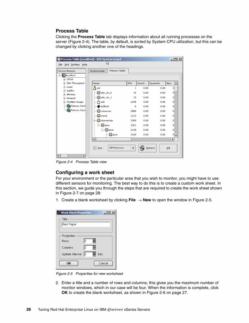
26 Tuning Red Hat Enterprise Linux on IBM Eserver xSeries Servers
Process TableClicking the Process Table tab displays information about all running processes on the server (Figure 2-4). The table, by default, is sorted by System CPU utilization, but this can be changed by clicking another one of the headings.
Figure 2-4 Process Table view
Configuring a work sheetFor your environment or the particular area that you wish to monitor, you might have to use different sensors for monitoring. The best way to do this is to create a custom work sheet. In this section, we guide you through the steps that are required to create the work sheet shown in Figure 2-7 on page 28:
1. Create a blank worksheet by clicking File → New to open the window in Figure 2-5.
Figure 2-5 Properties for new worksheet
2. Enter a title and a number of rows and columns; this gives you the maximum number of monitor windows, which in our case will be four. When the information is complete, click OK to create the blank worksheet, as shown in Figure 2-6 on page 27.

Chapter 2. Monitoring tools 27
Figure 2-6 Empty worksheet
3. Fill in the sensor boxes by dragging the sensors on the left side of the window to the desired box on the right. The types of display are:
– Signal Plotter: This displays samples of one or more sensors over time. If several sensors are displayed, the values are layered in different colors. If the display is large enough, a grid will be displayed to show the range of the plotted samples.
By default, the automatic range mode is active, so the minimum and maximum values will be set automatically. If you want fixed minimum and maximum values, you can deactivate the automatic range mode and set the values in the Scales tab from the Properties dialog window (which you access by right-clicking the graph).
– Multimeter: This displays the sensor values as a digital meter. In the Properties dialog, you can specify a lower and upper limit. If the range is exceeded, the display is colored in the alarm color.
– BarGraph: This displays the sensor value as dancing bars. In the Properties dialog, you can specify the minimum and maximum values of the range and a lower and upper limit. If the range is exceeded, the display is colored in the alarm color.
– Sensor Logger: This does not display any values, but logs them in a file with additional date and time information.
For each sensor, you have to define a target log file, the time interval the sensor will be logged, and whether alarms are enabled.
4. Click File → Save to save the changes to the worksheet.
Note: The fastest update interval that can be defined is two seconds.
Note: When you save a work sheet, it will be saved in the user’s home directory, which may prevent other administrators from using your custom worksheets.

28 Tuning Red Hat Enterprise Linux on IBM Eserver xSeries Servers
Figure 2-7 Example worksheet
Find more information about KDE System Guard at:
http://docs.kde.org/en/3.2/kdebase/ksysgaurd
2.11 Gnome System MonitorAlthough not as powerful as the KDE System Guard, the Gnome desktop environment features a graphical performance analysis tool. The Gnome System Monitor can display performance-relevant system resources as graphs for visualizing possible peaks and bottlenecks. Note that all statistics are generated in real time. Long-term performance analysis should be carried out with different tools.
2.12 freeThe command /bin/free displays information about the total amounts of free and used memory (including swap) on the system. It also includes information about the buffers and cache used by the kernel.
Example 2-11 Example output from the free command
total used free shared buffers cachedMem: 1291980 998940 293040 0 89356 772016-/+ buffers/cache: 137568 1154412Swap: 2040244 0 2040244

Chapter 2. Monitoring tools 29
When using free, remember the Linux memory architecture and the way the virtual memory manager works. The amount of free memory in itself is of limited use, and the pure utilization statistics of swap are no indication for a memory bottleneck.
Useful parameters for the free command include:
� -b, -k, -m, and -g display values in bytes, kilobytes, megabytes, and gigabytes.
� -l distinguishes between low and high memory (refer to 1.2, “The Linux memory architecture” on page 4).
� -c {count} displays the free output {count} number of times.
2.13 pmapThe pmap command reports the amount of memory that one or more processes are using. You can use this tool to determine which processes on the server are being allocated memory and whether this amount of memory is a cause of memory bottlenecks:
pmap <pid>
Example 2-12 Total amount of memory the smbd process is using
[root@x232 root]# pmap 8359smbd[8359]b723c000 (1224 KB) r-xp (08:02 1368219) /lib/tls/libc-2.3.2.sob736e000 (16 KB) rw-p (08:02 1368219) /lib/tls/libc-2.3.2.somapped: 9808 KB writable/private: 1740 KB shared: 64 KB
For the complete syntax of the pmap command, issue:
pmap -?
2.14 straceThe strace command intercepts and records the system calls that are called by a process, as well as the signals that are received by a process. This is a useful diagnostic, instructional, and debugging tool. System administrators find it valuable for solving problems with programs.
To use the command, specify the process ID (PID) to be monitored:
strace -p <pid>
Example 2-13 shows an example of the output of strace.
Example 2-13 Output of strace monitoring httpd process
[root@x232 html]# strace -p 815Process 815 attached - interrupt to quitsemop(360449, 0xb73146b8, 1) = 0poll([{fd=4, events=POLLIN}, {fd=3, events=POLLIN, revents=POLLIN}], 2, -1) = 1accept(3, {sa_family=AF_INET, sin_port=htons(52534), sin_addr=inet_addr("9.42.171.197")}, [16]) = 13semop(360449, 0xb73146be, 1) = 0getsockname(13, {sa_family=AF_INET, sin_port=htons(80), sin_addr=inet_addr("9.42.171.198")}, [16]) = 0fcntl64(13, F_GETFL) = 0x2 (flags O_RDWR)fcntl64(13, F_SETFL, O_RDWR|O_NONBLOCK) = 0read(13, 0x8259bc8, 8000) = -1 EAGAIN (Resource temporarily unavailable)poll([{fd=13, events=POLLIN, revents=POLLIN}], 1, 300000) = 1

30 Tuning Red Hat Enterprise Linux on IBM Eserver xSeries Servers
read(13, "GET /index.html HTTP/1.0\r\nUser-A"..., 8000) = 91gettimeofday({1084564126, 750439}, NULL) = 0stat64("/var/www/html/index.html", {st_mode=S_IFREG|0644, st_size=152, ...}) = 0open("/var/www/html/index.html", O_RDONLY) = 14mmap2(NULL, 152, PROT_READ, MAP_SHARED, 14, 0) = 0xb7052000writev(13, [{"HTTP/1.1 200 OK\r\nDate: Fri, 14 M"..., 264}, {"<html>\n<title>\n RedPaper Per"..., 152}], 2) = 416munmap(0xb7052000, 152) = 0socket(PF_UNIX, SOCK_STREAM, 0) = 15connect(15, {sa_family=AF_UNIX, path="/var/run/.nscd_socket"}, 110) = -1 ENOENT (No such file or directory)close(15) = 0
For the complete syntax of the strace command, issue:
strace -?
2.15 ulimitThis command is built into the bash shell and is used to provide control over the resources available to the shell and to the processes started by it on systems that allow such control.
Use the -a option to list all parameters that we can set:
ulimit -a
Example 2-14 Output of ulimit
[root@x232 html]# ulimit -acore file size (blocks, -c) 0data seg size (kbytes, -d) unlimitedfile size (blocks, -f) unlimitedmax locked memory (kbytes, -l) 4max memory size (kbytes, -m) unlimitedopen files (-n) 1024pipe size (512 bytes, -p) 8stack size (kbytes, -s) 10240cpu time (seconds, -t) unlimitedmax user processes (-u) 7168virtual memory (kbytes, -v) unlimited
The -H and -S options specify the hard and soft limits that can be set for the given resource. If the soft limit is passed, the system administrator will receive a warning. The hard limit is the maximum value that can be reached before the user gets the error messages Out of file handles.
For example, you can set a hard limit for the number of file handles and open files (-n):
ulimit -Hn 4096
For the soft limit of number of file handles and open files, use:
ulimit -Sn 1024
Attention: While the strace command is running against a process, the performance of the PID is drastically reduced and should only be run for the time of data collection.

Chapter 2. Monitoring tools 31
To see the hard and soft values, issue the command with a new value:
ulimit -Hnulimit -Sn
This command can be used, for example, to limit Oracle users on the fly. To set it on startup, enter the following lines, for example, in /etc/security/limits.conf:
soft nofile 4096hard nofile 10240
In addition, make sure that the /etc/pam.d/system-auth file has the following entry:
session required /lib/security/$ISA/pam_limits.so
This entry is required so that the system can enforce these limits.
For the complete syntax of the ulimit command, issue:
ulimit -?
2.16 mpstatThe mpstat utility is part of the sysstat package. If you not have installed this package, search for the sysstat rpm in your Red Hat Enterprise Linux sources and install it.
The mpstat command is used to report the activities of each of the available CPUs on a multiprocessor server. Global average activities among all CPUs are also reported.
The mpstat utility enables you to display overall CPU statistics per system or per processor. mpstat also enables the creation of statistics when used in sampling mode analogous to the vmstat command with a sampling frequency and a sampling count. Example 2-15 shows a sample output created with mpstat -P ALL to display average CPU utilization per processor.
Example 2-15 Output of mpstat command on multiprocessor system
[root@linux ~]# mpstat -P ALLLinux 2.6.9-5.ELsmp (linux.itso.ral.ibm.com) 04/22/2005
03:19:21 PM CPU %user %nice %system %iowait %irq %soft %idle intr/s03:19:21 PM all 0.03 0.00 0.34 0.06 0.02 0.08 99.47 1124.2203:19:21 PM 0 0.03 0.00 0.33 0.03 0.04 0.15 99.43 612.1203:19:21 PM 1 0.03 0.00 0.36 0.10 0.01 0.01 99.51 512.09
To display three entries of statistics for all processors of a multiprocessor server at one-second intervals, use the command:
mpstat -P ALL 1 2

32 Tuning Red Hat Enterprise Linux on IBM Eserver xSeries Servers
Example 2-16 Output of mpstat command on two-way machine
[root@linux ~]# mpstat -P ALL 1 2Linux 2.6.9-5.ELsmp (linux.itso.ral.ibm.com) 04/22/2005
03:31:51 PM CPU %user %nice %system %iowait %irq %soft %idle intr/s03:31:52 PM all 0.00 0.00 0.00 0.00 0.00 0.00 100.00 1018.8103:31:52 PM 0 0.00 0.00 0.00 0.00 0.00 0.00 100.00 991.0903:31:52 PM 1 0.00 0.00 0.00 0.00 0.00 0.00 99.01 27.72
Average: CPU %user %nice %system %iowait %irq %soft %idle intr/sAverage: all 0.00 0.00 0.00 0.00 0.00 0.00 100.00 1031.89Average: 0 0.00 0.00 0.00 0.00 0.00 0.00 100.00 795.68Average: 1 0.00 0.00 0.00 0.00 0.00 0.00 99.67 236.54
For the complete syntax of the mpstat command, issue:
mpstat -?
2.17 Capacity ManagerCapacity Manager, an add-on to the IBM Director system management suite for IBM eServers, is available in the ServerPlus Pack for IBM eServer xSeries systems. Capacity Manager offers the possibility of long-term performance measurements across multiple systems and platforms. Apart from performance measurement, Capacity Manager enables capacity planning, offering you an estimate of future required system capacity needs. With Capacity Manager, you can export reports to HTML, XML, and GIF files that can be stored automatically on an intranet Web server. IBM Director can be used on different operating system platforms, which makes it much easier to collect and analyze data in a heterogeneous environment. Capacity Manager is discussed in detail in the redbook Tuning IBM Eserver xSeries Servers for Performance, SG24-5287.
To use Capacity Manager, you first must install the respective RPM package on the systems that will use its advanced features. After installing the RPM, select Capacity Manager → Monitor Activator in the IBM Director Console.
Figure 2-8 The task list in the IBM Director Console
Drag and drop the icon for Monitor Activator over a single system or a group of systems that have the Capacity Manager package installed. A window opens (Figure 2-9 on page 33) in which you can select the various subsystems to be monitored over time. Capacity Manager for Linux does not yet support the full-feature set of available performance counters. System statistics are limited to a basic subset of performance parameters.
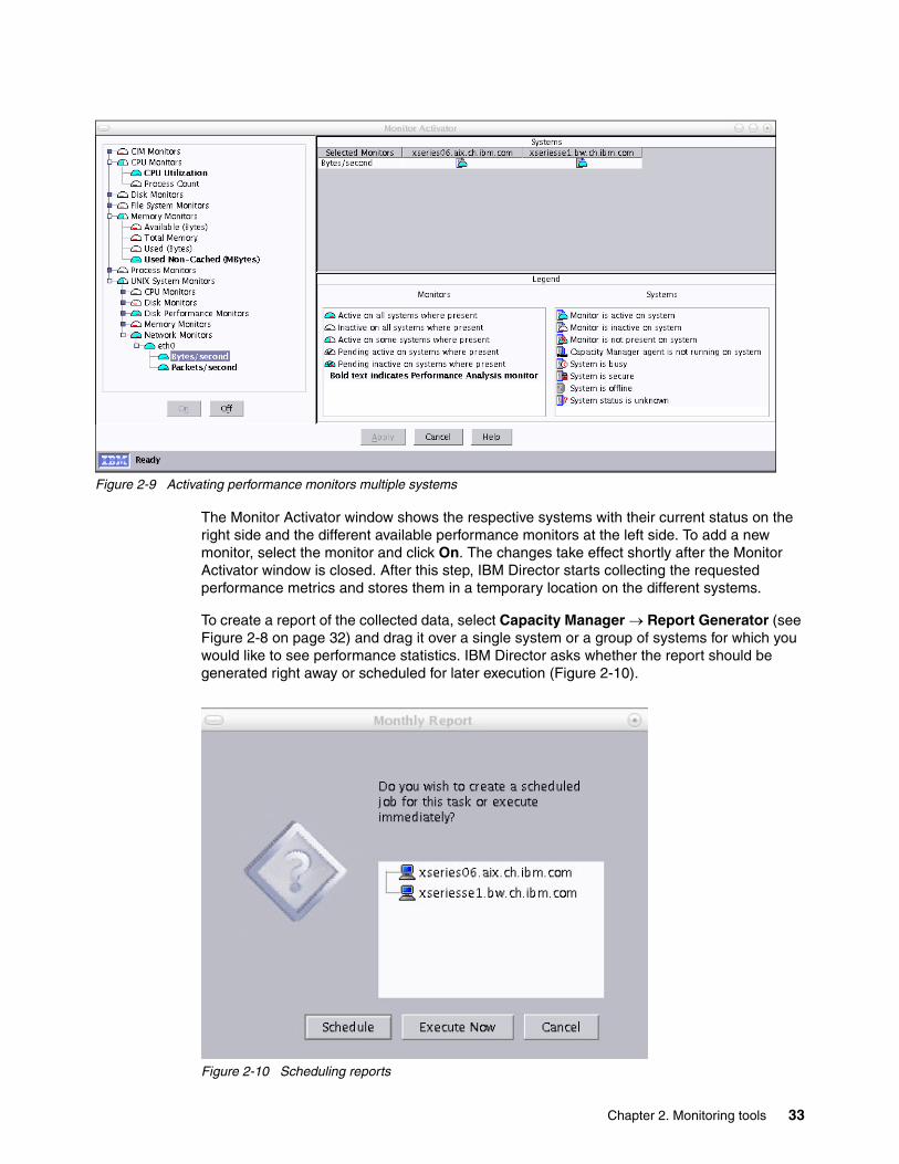
Chapter 2. Monitoring tools 33
Figure 2-9 Activating performance monitors multiple systems
The Monitor Activator window shows the respective systems with their current status on the right side and the different available performance monitors at the left side. To add a new monitor, select the monitor and click On. The changes take effect shortly after the Monitor Activator window is closed. After this step, IBM Director starts collecting the requested performance metrics and stores them in a temporary location on the different systems.
To create a report of the collected data, select Capacity Manager → Report Generator (see Figure 2-8 on page 32) and drag it over a single system or a group of systems for which you would like to see performance statistics. IBM Director asks whether the report should be generated right away or scheduled for later execution (Figure 2-10).
Figure 2-10 Scheduling reports

34 Tuning Red Hat Enterprise Linux on IBM Eserver xSeries Servers
In a production environment, it is a good idea to have Capacity Manager generate reports on a regular basis. Our experience is that weekly reports that are performed in off-hours over the weekend can be very valuable. An immediate execution or scheduled execution report is generated according to your choice. As soon as the report has completed, it is stored on the central IBM Director management server, where it can be viewed using the Report Viewer task. Figure 2-11 shows sample output from a monthly Capacity Manager report.
Figure 2-11 A sample Capacity Manager report
The Report Viewer window enables you to select the different performance counters that were collected and correlate this data to a single system or to a selection of systems.
Data acquired by Capacity Manager can be exported to an HTML or XML file to be displayed on an intranet Web server or for future analysis.

© Copyright IBM Corp. 2005. All rights reserved. 35
Chapter 3. Tuning the operating system
By its nature and heritage, the Linux distributions and the Linux kernel offer a variety of parameters and settings to let the Linux administrator tweak the system to maximize performance.
This chapter describes the steps you can take to tune Red Hat Enterprise Linux AS. The objective is to describe the parameters that give you the most improvement in performance and offer basic understanding of the techniques that are used in Linux, including:
� Linux memory management
� Page partitions in Linux
� File systems and their effect on performance
� Disabling unnecessary daemons
� Tuning parameters using sysctl
This chapter has the following sections:
� 3.1, “Change management” on page 36� 3.2, “Installation” on page 36� 3.3, “Daemons” on page 38� 3.4, “Changing run levels” on page 40� 3.7, “Compiling the kernel” on page 43� 3.8, “Changing kernel parameters” on page 44� 3.9, “Kernel parameters” on page 46� 3.10, “Tuning the processor subsystem” on page 47� 3.10, “Tuning the processor subsystem” on page 47� 3.11, “Tuning the memory subsystem” on page 50� 3.12, “Tuning the file system” on page 52� 3.14, “Tuning the network subsystem” on page 61
3

36 Tuning Red Hat Enterprise Linux on IBM Eserver xSeries Servers
3.1 Change managementWhile not strictly related to performance tuning, change management is probably the single most important factor for successful performance tuning. The following considerations might be second nature to you, but as a reminder we highlight these points:
� Implement a proper change management process before tuning any Linux system.
� Never start tweaking settings on a production system.
� Never change more than one variable during the tuning process.
� Retest parameters that supposedly improved performance; sometimes statistics come into play.
� Document successful parameters and share them with the community no matter how trivial you think they are. Linux performance is a topic that can benefit greatly from any results obtained in production environments.
3.2 InstallationIn a perfect world, tuning of any given system starts at a very early stage. Ideally a system is tailored to the needs of the application and the anticipated workload. We understand that most of the time an administrator has to tune an already installed system due to a bottleneck, but we also want to highlight the tuning possibilities available during the initial installation of the operating system.
Several issues should be resolved before starting the installation of Linux, including:
� Selection of the processor technology � Choice of disk technology� Applications
However, these issues are beyond the scope of this book. See the IBM Redbook Tuning IBM Eserver xSeries Servers for Performance, SG24-5287 to address these issues.
Ideally, the following questions should be answered before starting the installation.
� What version of Red Hat Linux do I need?
After you have collected the business and application requirements, decide which version of Linux to use. Enterprises often have contractual agreements that allow the general use of a specific Linux distribution. In this case, financial and contractual benefits will most likely dictate the version of Linux that can be used. However, if you have full freedom in choosing the version of Red Hat Enterprise Linux, there are some points to consider:
– A supported enterprise Linux or a custom made distribution?
In certain scientific environments it is acceptable to run an unsupported version of Linux, such as Fedora. For enterprise workloads, we strongly recommend a fully supported distribution such as Red Hat Enterprise Linux.
– What version of an enterprise distribution?
Red Hat Enterprise Linux comes in two flavors: the Enterprise Server and the Advanced Server. The two versions differ mainly in scalability, with the Enterprise Server limited to two processors and 16 GB of memory. Therefore, the Enterprise Server is the right choice for edge systems such as Web servers and distributed architectures. The Advanced Server version of Red Hat Enterprise Linux supports up to 32 processors (for Intel IA-32 and x86-64 systems) and up to 64 GB of memory (again speaking of Intel IA-32 and x86-64 systems).

Chapter 3. Tuning the operating system 37
With the advent of x86-64 architectures (AMD64 or EM64T respectively), clients also have the choice of running a 32-bit or 64-bit version of the OS on the system. Our benchmarks have shown that Linux systems run faster using a 64-bit operating system on an x86-64 CPU. Apart from performance, scalability and support for future applications might be of concern. Running a 64-bit operating system provides the advantage of being able to run both 32-bit applications (i386 binaries) and 64-bit applications (x86-64 binaries) at the same time. Considering all of these points, we generally suggest the use of a 64-bit operating system on x86-64 architectures unless application support hinders the deployment of a 64-bit environment.
� What partition layout to choose?
In the Linux community, the partitioning of a disk subsystem engenders vast discussion. The partitioning layout of a disk subsystem is often dictated by application needs, systems management considerations, and personal liking, and not performance. The partition layout will therefore be given in most cases. The only suggestion we want to give here is to use a swap partition if possible. Swap partitions, as opposed to swap files, have a performance benefit because there is no overhead of a file system. Swap partitions are simple and can be expanded with additional swap partitions or even swap files if needed.
� What file system to use?
The installation of Red Hat Enterprise Linux limits the choice of file systems because only two file systems are available during installation: ext2 and ext3. The Red Hat Enterprise Linux installer defaults to ext3 and this is acceptable in most cases, but we encourage you to consider using ext2. Smaller file systems that have no focus on integrity (for example, a Web server cluster) and systems with a strict need for performance (high-performance computing environments) can benefit from the performance of the ext2 file system. ext2 does not have the overhead of journaling, and even if ext3 has undergone tremendous improvements, there still is a difference. Also note that ext2 file systems can be upgraded easily to ext3.
� Package selection: minimal or everything?
During an installation of Red Hat Enterprise Linux, administrators are faced with the decision of a minimal-or-everything installation approach. Philosophies differ somewhat in this area. There are voices that prefer everything installations because there is hardly ever the need to install packages to resolve dependencies.
Consider these points: While not related to performance, it is important to point out that an “everything” or “near-everything” installation imposes security threats on a system. The availability of development tools on production systems may lead to significant security threats. The fewer packages you install, the less disk space will be wasted, and a disk with more free space performs better than a disk with little free space. Intelligent software installers such as the Red Hat Packet Manager or rpm or yum will resolve dependencies automatically if desired. Therefore, we suggest you consider a minimal packet selection with only those packages that are absolutely necessary for a successful implementation of the application.
� SELinux (Red Hat Enterprise Linux 4 only)
In Red Hat Enterprise Linux, the Anaconda installer defaults to the installation of SELinux. However, SELinux comes at a significant performance penalty and you should carefully evaluate whether the additional security provided by SELinux is really needed for a particular system. For more information, refer to 3.6, “SELinux” on page 42.
� Run level selection
The last choice given during the installation process is the selection of the run level your system defaults to. Unless you have a specific need to run your system in runlevel 5 (graphical user mode) we strongly suggest using runlevel 3 for all server systems.

38 Tuning Red Hat Enterprise Linux on IBM Eserver xSeries Servers
Normally there should be no need for a GUI on a system that resides in a data center, and the overhead imposed by runlevel 5 is considerable.
3.3 DaemonsAfter a default installation of Red Hat Enterprise Linux, several possibly unnecessary services and daemons might be enabled. Disabling unneeded daemons reduces the overall memory footprint of the system and, more important, reduces exposure to various security threats. Disabling unneeded daemons frees memory and decreases startup time and the number of processes that the CPU has to handle.
By default, several daemons that have been started can be stopped and disabled safely on most systems. Table 3-1 lists the daemons that are started in Red Hat Enterprise Linux installations. You should consider disabling these in your environment if applicable. Note that the table lists the respective daemons for Red Hat Enterprise Linux Version 3 and Version 4. For a more detailed explanation of these daemons, refer to the redhat-config-services GUI shown in Figure 3-1 on page 40.
Table 3-1 Tunable daemons started on a default installation
Daemons RHEL 3 RHEL 4 Description
apmd X X Advanced power management daemon. apmd will most likely not be used on a server.
arptables_jf X User space program for the arptables network filter. Unless you plan to use arptables, you can safely disable this daemon.
autofs X X Automatically mounts file systems on demand (for example, mounts a CD-ROM automatically). On server systems, file systems rarely have to be mounted automatically.
cpuspeed X Daemon to dynamically adjust the frequency of the CPU. In a server environment, this daemon is recommended off.
cups X X Common UNIX Printing System. If you plan to provide print services with your server, do not disable this service.
gpm Mouse server for the text console. Do not disable if you want mouse support for the local text console.
hpoj X HP OfficeJet support. Do not disable if you plan to use an HP OfficeJet printer with your server.
irqbalance X Balances interrupts between multiple processors. You may safely disable this daemon on a singe CPU system or if you plan to balance IRQ statically.
isdn X X ISDN modem support. Do not disable if you plan to use an ISDN modern with your server.
kudzu X X Detects and configures new hardware. Should be run manually in case of a hardware change.
netfs X X Used in support of exporting NFS shares. Do not disable if you plan to provide NFS shares with your server.
nfslock X X Used for file locking with NFS. Do not disable if you plan to provide NFS shares with your server.
pcmcia X X PCMCIA support on a server. Server systems rarely rely on a PCMCIA adapter so disabling this daemon is safe in most instances.
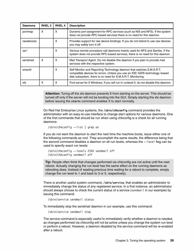
Chapter 3. Tuning the operating system 39
On Red Hat Enterprise Linux systems, the /sbin/chkconfig command provides the administrator with an easy-to-use interface to change start options for various daemons. One of the first commands that should be run when using chkconfig is a check for all running daemons:
/sbin/chkconfig --list | grep on
If you do not want the daemon to start the next time the machine boots, issue either one of the following commands as root. They accomplish the same results, the difference being that the second command disables a daemon on all run levels, whereas the --level flag can be used to specify exact run levels:
/sbin/chkconfig --levels 2345 sendmail off /sbin/chkconfig sendmail off
There is another useful system command, /sbin/service, that enables an administrator to immediately change the status of any registered service. In a first instance, an administrator should always choose to check the current status of a service (sendmail in our example) by issuing this command:
/sbin/service sendmail status
To immediately stop the sendmail daemon in our example, use this command:
/sbin/service sendmail stop
The service command is especially useful to immediately verify whether a daemon is needed, as changes performed via chkconfig will not be active unless you change the system run level or perform a reboot. However, a daemon disabled by the service command will be re-enabled after a reboot.
portmap X X Dynamic port assignment for RPC services (such as NIS and NFS). If the system does not provide RPC-based services there is no need for this daemon.
rawdevices X Provides support for raw device bindings. If you do not intend to use raw devices you may safely turn it off.
rpc* X Various remote procedure call daemons mainly used for NFS and Samba. If the system does not provide RPC-based services, there is no need for this daemon.
sendmail X X Mail Transport Agent. Do not disable this daemon if you plan to provide mail services with the respective system.
smartd X Self Monitor and Reporting Technology daemon that watches S.M.A.R.T. compatible devices for errors. Unless you use an IDE/ SATA technology–based disk subsystem, there is no need for S.M.A.R.T. Monitoring.
xfs X X Font server for X Windows. If you will run in runlevel 5, do not disable this daemon.
Daemons RHEL 3 RHEL 4 Description
Attention: Turing off the xfs daemon prevents X from starting on the server. This should be turned off only if the server will not be booting into the GUI. Simply starting the xfs daemon before issuing the startx command enables X to start normally.
Tip: People often think that changes performed via chkconfig are not active until the next reboot. Actually changing the run level has the same effect on the running daemons as rebooting does. Instead of wasting precious time waiting for a reboot to complete, simply change the run level to 1 and back to 3 or 5, respectively).

40 Tuning Red Hat Enterprise Linux on IBM Eserver xSeries Servers
Similarly, there is a GUI-based program for modifying which daemons are started, as shown in Figure 3-1. To run the GUI, click Main Menu → System Settings → Server Settings → Services or issue this command:
/usr/bin/redhat-config-services
Figure 3-1 Red Hat Service Configuration interface
3.4 Changing run levelsWhenever possible, do not run the graphical user interface on a Linux server. Normally, there is no need for a GUI on a Linux server, as most Linux administrators will happily assure you. All administrative tasks can be achieved efficiently via the command line, by redirecting the X display, or through a Web browser interface. If you prefer a graphical interface, there are several useful Web-based tools such as webmin, Linuxconf, and SWAT.
If a GUI must be used, start and stop it as needed rather than running it all the time. In most cases the server should be running at runlevel 3, which does not start the X Server when the machine boots up. If you want to restart the X Server, use startx from a command prompt.
1. Determine which run level the machine is running by using the runlevel command.
This prints the previous and current run level. For example, N 5 means that there was no previous run level (N) and that the current run level is 5.
2. To switch between run levels, use the init command. (For example, to switch to runlevel 3, enter the init 3 command.
The run levels that are used in Linux are:
0 Halt (Do not set initdefault to this or the server will shut down immediately after finishing the boot process.)
1 Single user mode
2 Multiuser, without NFS (the same as 3, if you do not have networking)
To change the current state, highlight the daemon and click Stop.
The check mark indicates the daemon will start at the next reboot.
Tip: Even if the GUI is disabled locally on the server, you can still connect remotely and use the GUI. To do this, use the -X parameter with the ssh command.
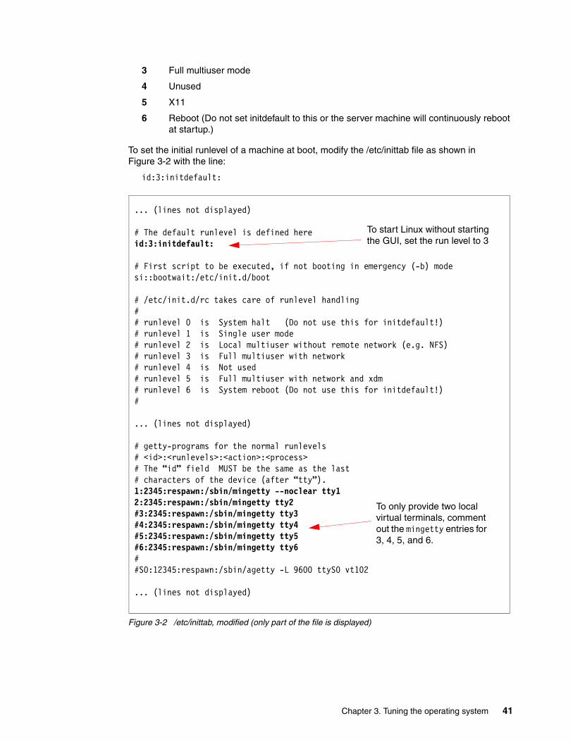
Chapter 3. Tuning the operating system 41
3 Full multiuser mode
4 Unused
5 X11
6 Reboot (Do not set initdefault to this or the server machine will continuously reboot at startup.)
To set the initial runlevel of a machine at boot, modify the /etc/inittab file as shown in Figure 3-2 with the line:
id:3:initdefault:
Figure 3-2 /etc/inittab, modified (only part of the file is displayed)
To start Linux without starting the GUI, set the run level to 3
To only provide two local virtual terminals, comment out the mingetty entries for 3, 4, 5, and 6.
... (lines not displayed)
# The default runlevel is defined hereid:3:initdefault:
# First script to be executed, if not booting in emergency (-b) modesi::bootwait:/etc/init.d/boot
# /etc/init.d/rc takes care of runlevel handling## runlevel 0 is System halt (Do not use this for initdefault!)# runlevel 1 is Single user mode# runlevel 2 is Local multiuser without remote network (e.g. NFS)# runlevel 3 is Full multiuser with network# runlevel 4 is Not used# runlevel 5 is Full multiuser with network and xdm# runlevel 6 is System reboot (Do not use this for initdefault!)#
... (lines not displayed)
# getty-programs for the normal runlevels# <id>:<runlevels>:<action>:<process># The “id” field MUST be the same as the last# characters of the device (after “tty”).1:2345:respawn:/sbin/mingetty --noclear tty12:2345:respawn:/sbin/mingetty tty2#3:2345:respawn:/sbin/mingetty tty3#4:2345:respawn:/sbin/mingetty tty4#5:2345:respawn:/sbin/mingetty tty5#6:2345:respawn:/sbin/mingetty tty6##S0:12345:respawn:/sbin/agetty -L 9600 ttyS0 vt102
... (lines not displayed)

42 Tuning Red Hat Enterprise Linux on IBM Eserver xSeries Servers
3.5 Limiting local terminalsBy default, six virtual consoles are spawned locally: Keys F1 through F6 provide access to separate consoles. The amount of memory used by the virtual terminals is negligible; nevertheless we try to get the most out of any system. Additionally, troubleshooting and process analysis will be simplified by simply reducing the amount of running processes, hence the reason for limiting the local terminals to two.
To do this, comment out each mingetty ttyx line you want to disable. As an example, in Figure 3-2 on page 41 we limited the consoles to two. This gives you a fallback local terminal in case a command kills the shell you were working on locally.
3.6 SELinuxRed Hat Enterprise Linux 4 introduced a new security model, Security Enhanced Linux (SELinux), which is a significant step toward higher security. SELinux introduces a mandatory policy model that overcomes the limitations of the standard discretionary access model employed by Linux. SELinux enforces security on user and process levels; hence a security flaw of any given process affects only the resources allocated to this process and not the entire system. SELinux works similar to a virtual machine. For example, if a malicious attacker uses a root exploit within Apache, only the resources allocated to the Apache daemon could be compromised.
Figure 3-3 Schematic overview of SELinux
However, enforcing such a policy-based security model comes at a price. Every access from a user or process to a system resource such as an I/O device must be controlled by SELinux. The process of checking permissions can cause overhead of up to 10%. SELinux is of great value to any edge server such as a firewall or a Web server, but the added level of security on a back-end database server may not justify the loss in performance.
Generally the easiest way to disable SELinux is to not install it in the first place. But often systems have been installed using default parameters, unaware that SELinux affects performance. To disable SELinux after an installation append the entry selinux=0 to the line containing the running kernel in the GRUB boot loader (Example 3-1 on page 43).
SELinux Kernel
SECURITYPOLICY
SECURITYENFORCEMENT
MODULE
Process
User
SYSTEMRESOURCES
RequestAccess
GrantAccess
Grant/Deny AccessBased on Policy
SELinux Kernel
SECURITYPOLICY
SECURITYENFORCEMENT
MODULE
Process
User
SYSTEMRESOURCES
RequestAccess
GrantAccess
Grant/Deny AccessBased on Policy

Chapter 3. Tuning the operating system 43
Example 3-1 Sample grub.conf file with disabled SELinux
default=0splashimage=(hd0,0)/grub/splash.xpm.gzhiddenmenutitle Red Hat Enterprise Linux AS (2.6.9-5.ELsmp) root (hd0,0) kernel /vmlinuz-2.6.9-5.ELsmp ro root=LABEL=/ selinux=0 initrd /initrd-2.6.9-5.ELsmp.img
If you decide to use SELinux with your Linux-based server, its settings can be tweaked to better accommodate your environment. On a running system, check whether the working set of the cached Linux Security Modules (LSM) permissions exceeds the default Access Vector Cache (AVC) size of 512 entries.
Check /selinux/avc/hash_stats for the length of the longest chain. Anything over 10 signals a likely bottleneck.
If the system experiences a bottleneck in the Access Vector Cache (for example, on a heavily loaded firewall), try to resize /selinux/avc/cache_threshold to a slightly higher value and recheck the hash stats.
3.7 Compiling the kernelCreating and compiling your own kernel has far less of an impact on improving system performance than often thought. Modern kernels shipped with most Linux distributions are modular—they load only the parts that are used. Recompiling the kernel can decrease kernel size and its overall behavior (for example, real-time behavior). Changing certain parameters in the source code might also yield some system performance. However, non-standard kernels are not covered in the support subscription that is provided with every Red Hat Enterprise Linux purchase. Additionally, the extensive ISV application and IBM hardware certifications that are provided for Red Hat Enterprise Linux are nullified if a non-standard kernel is used.
Having said that, performance improvements can be gained with a custom-made kernel, but they hardly justify the challenges you face running an unsupported kernel in an enterprise environment. While this is true for commercial workloads, if scientific workloads such as high performance computing are your area of interest, custom kernels might nevertheless be of interest to you.
Also do not attempt to use special compiler flags such as -C09 when recompiling the kernel. The source code for the Linux kernel has been hand-tuned to match the GNU C compiler. Using special compiler flags might at best decrease the kernel performance and at worst break the code.
Keep in mind that unless you really know what you are doing, you might actually decrease system performance due to wrong kernel parameters. If you understand these consequences and still wish to recompile the kernel, a complete discussion of how to compile the kernel is covered in the IBM Redpaper Running the Linux 2.4 Kernel on IBM ̂xSeries Servers, REDP0121, which is available from:
http://www.redbooks.ibm.com/abstracts/redp0121.html
Tip: To check for usage statistics of the access vector cache you may alternatively use the avcstat utility.

44 Tuning Red Hat Enterprise Linux on IBM Eserver xSeries Servers
3.8 Changing kernel parametersAlthough modifying and recompiling the kernel source code is not recommended for most users, the Linux kernel features yet another means of tweaking kernel parameters. The proc file system provides an interface to the running kernel that may be used for monitoring purposes and for changing kernel settings on the fly.
To view the current kernel configuration, choose a kernel parameter in the /proc/sys directory and use the cat command on the respective file. In Example 3-2 we parse the system for its current memory overcommit strategy. The output 0 tells us that the system will always check for available memory before granting an application a memory allocation request. To change this default behavior we can use the echo command and supply it with the new value, 1 in the case of our example (1 meaning that the kernel will grant every memory allocation without checking whether the allocation can be satisfied).
Example 3-2 Changing kernel parameters via the proc file system
[root@linux vm]# cat overcommit_memory0[root@linux vm]# echo 1 > overcommit_memory
While the demonstrated way of using cat and echo to change kernel parameters is fast and available on any system with the proc file system, it has two significant shortcomings.
� The echo command does not perform any consistency check on the parameters.� All changes to the kernel are lost after a reboot of the system.
To overcome this, a utility called sysctl aids the administrator in changing kernel parameters.
In addition, Red Hat Enterprise Linux 2 and 3 offer a graphical method of modifying these sysctl parameters. To launch the tool, issue the following command:
/usr/bin/redhat-config-proc
Figure 3-4 on page 45 shows the user interface.
Tip: By default, the kernel includes the necessary module to enable you to make changes using sysctl without having to reboot. However, If you chose to remove this support (during the operating system installation), then you will have to reboot Linux before the change will take effect.

Chapter 3. Tuning the operating system 45
Figure 3-4 Red Hat kernel tuning
3.8.1 Where the parameters are storedThe kernel parameters that control how the kernel behaves are stored in /proc (in particular, /proc/sys).
Reading the files in the /proc directory tree provides a simple way to view configuration parameters that are related to the kernel, processes, memory, network, and other components. Each process running in the system has a directory in /proc with the process ID (PID) as its name. Figure 3-2 lists some of the files that contain kernel information.
Table 3-2 Parameter files in /proc
File/directory Purpose
/proc/sys/abi/* Used to provide support for “foreign” binaries, not native to Linux — those compiled under other UNIX variants such as SCO UnixWare 7, SCO OpenServer, and SUN Solaris 2. By default, this support is installed, although it can be removed during installation.
/proc/sys/fs/* Used to increase the number of open files the OS allows and to handle quota.
/proc/sys/kernel/* For tuning purposes, you can enable hotplug, manipulate shared memory, and specify the maximum number of PID files and level of debug in syslog.
/proc/sys/net/* Tuning of network in general, IPV4 and IPV6.
/proc/sys/vm/* Management of cache memory and buffer.

46 Tuning Red Hat Enterprise Linux on IBM Eserver xSeries Servers
3.8.2 Using the sysctl commandThe sysctl command uses the names of files in the /proc/sys directory tree as parameters. For example, to modify the shmmax kernel parameter, you can display (using cat) and change (using echo) the file /proc/sys/kernel/shmmax:
#cat /proc/sys/kernel/shmmax 33554432 #echo 33554430 > /proc/sys/kernel/shmmax #cat /proc/sys/kernel/shmmax 33554430
However, using these commands can easily introduce errors, so we recommend that you use the sysctl command because it checks the consistency of the data before it makes any change. For example:
#sysctl kernel.shmmax kernel.shmmax = 33554432 #sysctl -w kernel.shmmax=33554430 kernel.shmmax = 33554430 #sysctl kernel.shmmax kernel.shmmax = 33554430
This change to the kernel stays in effect only until the next reboot. If you want to make the change permanently, then you can edit the /etc/sysctl.conf file and add the appropriate command. In our example:
kernel.shmmax = 33554439
The next time you reboot, the parameter file will be read. You can do the same thing without rebooting by issuing the following command:
#sysctl -p
3.9 Kernel parametersVersion 2.4 and 2.6 of the Linux kernel feature many parameters that can improve performance for your installation.
Table 3-3 lists the kernel parameters that are most relevant to performance. Table 3-4 on page 47 lists parameters that are relevant but not normally used in performance tuning.
Table 3-3 Red Hat parameters that are most relevant to performance tuning
Parameter Description and example of use
net.ipv4.inet_peer_gc_maxtime How often the garbage collector (gc) should pass over the inet peer storage memory pool during low or absent memory pressure. Default is 120, measured in jiffies.sysctl -w net.ipv4.inet_peer_gc_maxtime=240
net.ipv4.inet_peer_gc_mintime Sets the minimum time that the garbage collector can pass cleaning memory. If your server is heavily loaded, you may want to increase this value. Default is 10, measured in jiffies.sysctl -w net.ipv4.inet_peer_gc_mintime=80
net.ipv4.inet_peer_maxttl The maximum time-to-live for the inet peer entries. New entries will expire after this period of time. Default is 600, measured in jiffies.sysctl -w net.ipv4.inet_peer_maxttl=500

Chapter 3. Tuning the operating system 47
Table 3-4 Red Hat performance parameters that typically are not used
3.10 Tuning the processor subsystemIn any computer, be it a hand-held device or a cluster for scientific applications, the main subsystem is the processor that does the actual computing. During the past decade Moore’s Law has caused processor subsystems to evolve significantly faster than other subsystems have. The result is that now bottlenecks rarely occur within the CPU, unless number crunching is the sole purpose of the system. This is impressively illustrated by the average CPU utilization of an Intel-compatible server system that lies below 10%. Having said that, it is important to understand the bottlenecks that can occur at the processor level and to know possible tuning parameters in order to improve CPU performance.
net.ipv4.inet_peer_minttl The minimum time-to-live for inet peer entries. Set high enough to cover fragment time to live in the reassembling side of fragmented packets. This minimum time must be smaller than net.ipv4.inet_peer_threshold. Default is 120, measured in jiffies.sysctl -w net.ipv4.inet_peer_minttl=80
net.ipv4.inet_peer_threshold Set the size of inet peer storage. When this limit is reached, peer entries will be thrown away, using the inet_peer_gc_mintime timeout. Default is 65644.sysctl -w net.ipv4.inet_peer_threshold=65644
vm.hugetlb_pool The hugetlb feature works the same way as bigpages, but after hugetlb allocates memory, the physical memory can be accessed only by hugetlb or shm allocated with SHM_HUGETLB. It is normally used with databases such as Oracle or DB2®. Default is 0.sysctl -w vm.hugetlb_pool=4608
vm.inactive_clean_percent Designates the percent of inactive memory that should be cleaned. Default is 5%.sysctl -w vm.inactive_clean_percent=30
vm.pagecache Designates how much memory should be used for page cache. This is important for databases such as Oracle and DB2. Default is 1 15 100.This parameter’s three values are:� Minimum percent of memory used for page cache. Default is 1%.� The initial amount of memory for cache. Default is 15%.� Maximum percent of memory used for page cache. Default is 100%.sysctl -w vm.pagecache=1 50 100
Parameter Description and example of use
Parameter Description / example of use
kernel.panic_on_oops Enables kernel detection and handling of any process that causes a crash and calls the panic() function at the end. The kernel.panic parameter must also be set to 1. Default is 1 (enable).sysctl -w kernel.panic_on_oops=0
kernel.pid_max Determines the maximum PID that a process can allocate. Default is 32768.sysctl -w kernel.pid_max=65536
net.ipv4.tcp_tw_recycle The main states of TCP connection are ESTABLISHED, TIME_WAIT, and CLOSED. This parameter enables the fast recycling function of TIME-WAIT sockets. Default is 0 (disable).sysctl -w net.ipv4.tcp_tw_recycle=10
vm.overcommit_ratio Percentage of memory that is allowed for overcommit. Default is 50%.sysctl -w vm.overcommit_ratio=17

48 Tuning Red Hat Enterprise Linux on IBM Eserver xSeries Servers
On high-end servers with Xeon processors, you may wish to enable or disable Hyper-Threading.
Hyper-Threading represents each physical CPU as two processors to the operating system. This technique often referred to as symmetric multithreading (SMT) is fully supported by newer Linux kernels. By using SMT on the processor you can execute two threads or processes at a time (also know as thread-level parallelism). By having your OS and software designed to take advantage of this technology you can gain significant increases in performance without requiring an increase in clock speed.
For example, if you have Hyper-Threading enabled on a 4-way server, monitoring tools such as top will display eight processors. See Figure 3-5.
Figure 3-5 Output of top on a four-way server with Hyper-Threading enabled
Note with respect to Hyper-Threading:
� SMP-based kernels are required to support Hyper-Threading.
� The more CPUs installed in a server, the less benefit Hyper-Threading has on performance. On servers that are CPU-bound, expect, at most, the following performance gains:
– Two physical processors: 15-25% performance gain– Four physical processors: 1-13% gain– Eight physical processors: 0-5% gain
For more information about Hyper-Threading, see:
http://www.intel.com/business/bss/products/hyperthreading/server/
EM64T is a 64-bit extension to Intel IA-32 processors, which means that the processors are capable of addressing more memory and can support new 64-bit applications while remaining fully compatible with all existing 32-bit applications. Support for this new processor is in Red Hat Enterprise Linux 3 Update 2.
For more information about EM64T, see:
http://www.intel.com/technology/64bitextensions/
10:22:45 up 23:40, 5 users, load average: 26.49, 12.03, 10.24373 processes: 370 sleeping, 2 running, 1 zombie, 0 stoppedCPU states: cpu user nice system irq softirq iowait idle total 36.1% 0.1% 9.7% 0.3% 4.1% 1.6% 47.7% cpu00 17.0% 0.0% 5.9% 3.1% 20.8% 2.1% 50.7% cpu01 54.9% 0.0% 10.9% 0.0% 0.9% 1.3% 31.7% cpu02 33.4% 0.1% 8.5% 0.0% 2.5% 0.9% 54.2% cpu03 33.8% 0.7% 10.0% 0.0% 0.9% 2.1% 52.0% cpu04 31.4% 0.0% 9.3% 0.0% 2.9% 2.5% 53.6% cpu05 33.4% 0.0% 9.9% 0.0% 2.1% 0.7% 53.6% cpu06 30.5% 0.0% 11.1% 0.0% 1.7% 1.3% 55.1% cpu07 54.5% 0.0% 12.1% 0.0% 0.5% 1.9% 30.7%Mem: 8244772k av, 3197880k used, 5046892k free, 0k shrd, 91940k buff 2458344k active, 34604k inactiveSwap: 2040244k av, 0k used, 2040244k free 1868016k cached

Chapter 3. Tuning the operating system 49
3.10.1 Selecting the correct kernelRed Hat Enterprise Linux ASincludes several kernel packages, as listed in Table 3-5. For performance reasons, be sure to select the most appropriate kernel for your system.
Table 3-5 Available kernels in the distribution
3.10.2 Interrupt handlingOne of the highest-priority tasks a CPU has to handle is interrupts. Interrupts may be caused by subsystems such as a network interface card. Hard interrupts cause a CPU to stop its current work and perform a context switch, which is undesirable because the processor has to flush its cache to make room for the new work. (Think of a processor’s cache as a work bench that has to be cleaned up and supplied with new tools every time new work has to be done.) Two principles have proven to be most efficient when it comes to interrupt handling.
� Bind processes that cause a significant amount of interrupts to a CPU.
CPU affinity enables the system administrator to bind interrupts to a group or a single physical processor (of course, this does not apply on a single-CPU system). To change the affinity of any given IRQ, go into /proc/irq/%{number of respective irq}/ and change the CPU mask stored in the file smp_affinity. To set the affinity of IRQ 19 to the third CPU in a system (without SMT) use the command in Example 3-3.
Example 3-3 Setting the CPU affinity for interrupts
[root@linux /]#echo 03 > /proc/irq/19/smp_affinity
� Let physical processors handle interrupts.
In SMT systems such as Intel Xeon™ processors supporting Hyper-Threading, it is suggested that you bind interrupt handling to the physical processor rather than the SMT instance. The physical processors usually have the lower CPU numbering so in a two-way system with Hyper-Threading enabled, CPU ID 0 and 2 would refer to the physical CPU, and 1 and 3 would refer to the Hyper Threading instances. If you do not use the smp_affinity flag, you will not have to worry about this.
3.10.3 Considerations for NUMA systemsNon-Uniform Memory Access (NUMA) systems are gaining market share and are seen as the natural evolution of classic symmetric multiprocessor systems. Although the CPU scheduler used by current Linux distributions is well suited for NUMA systems, applications might not always be. Bottlenecks caused by a non-NUMA-aware application can cause performance degradations that are hard to identify. The recent numastat utility shipped in the numactl package helps to identify processes that have difficulties dealing with NUMA architectures.
To help with spotting bottlenecks, statistics provided by the numastat tool are available in the /sys/devices/system/node/%{node number}/numastat file. High values in numa_miss and the other_node field signal a likely NUMA issue. If you find that a process is allocated memory that does not reside on the local node for the process (the node that holds the processors that run the application), try to renice the process to the other node or work with NUMA affinity.
Kernel type Description
SMP Kernel has support for SMP and Hyper-Threaded machines.
Hugemem Support for machines with greater than 12 GB of memory. Includes support for NUMA.
Standard Single processor machines.

50 Tuning Red Hat Enterprise Linux on IBM Eserver xSeries Servers
3.11 Tuning the memory subsystemTuning the memory subsystem is a difficult task that requires constant monitoring to ensure that changes do not negatively affect other subsystems in the server. If you do choose to modify the virtual memory parameters (in /proc/sys/vm), we recommend that you change only one parameter at a time and monitor how the server performs.
Remember that most applications under Linux do not write directly to the disk, but to the file system cache maintained by the virtual memory manager that will eventually flush out the data. When using an IBM ServeRAID controller or an IBM TotalStorage® disk subsystem, you should try to the decrease the number of flushes, effectively increasing the I/O stream caused by each flush. The high-performance disk controller can handle the larger I/O stream more efficiently than multiple small ones.
3.11.1 Configuring bdflush (kernel 2.4 only)There is tuning in the virtual memory subsystem that can help improve overall file system performance. The bdflush kernel daemon is responsible for making sure that dirty buffers, any modified data that currently resides only in the volatile system memory, are committed to disk. Changes in the /proc system take effect immediately but will be reset at boot time. To make changes permanent, include the echo or sysctl command in the /etc/rc.d/rc.local file.
Configuring how the Linux kernel will flush dirty buffers to disk can tailor the flushing algorithm toward the specifications of the respective disk subsystem. Disk buffers are used to cache data that is stored on disks, which are very slow compared with RAM. So, if the server uses this kind of memory, it can create serious problems with performance. By modifying the /proc/sys/vm/bdflush parameters, you can modify the writing-to-disk rate, possibly avoiding disk contention problems. To edit the parameters of the bdflush subsystem, you may use either the echo command or sysctl, though we strongly encourage you to use sysclt.
Example 3-4 Using sysctl to change parameters of bdflush
sysctl -w vm.bdflush="30 500 0 0 500 3000 60 20 0"
The nine parameters in the /proc/sys/vm/bdflush of 2.4 Linux kernels are:
nfract Maximum percentage of dirty buffers in the buffer cache. The higher the value, the longer the write to the disk will be postponed. When available memory is in short supply, large amounts of I/O will have to be processed. To spread I/O out evenly, keep this a low value.
ndirty Maximum number of dirty buffers that the bdflush process can write to disk at one time. A large value results in I/O occurring in bursts, and a small value may lead to memory shortages if the bdflush daemon is not executed enough.
dummy2 Unused (formerly nrefill)
dummy3 Unused
interval Minimum rate at which kupdate will wake and flush. Default is 5 seconds, with a minimum value of zero seconds and a maximum of 600 seconds.
age_buffer Maximum time the OS will wait before writing buffer cache to disk. Default is 30 seconds, with minimum of 1 second and maximum of 6000 seconds.
nfract_sync Percent of dirty buffers to activate bdflush synchronously. Default is 60%.
nfract_stop Percent of dirty buffers to stop bdflush. Default is 20%.
dummy5 Unused

Chapter 3. Tuning the operating system 51
Example 3-5 Modifying the bdflush parameters in the kernel using echo
echo 30 500 0 0 500 30000 60 20 0 > /proc/sys/vm/bdflush
3.11.2 Configuring kswapd (kernel 2.4 only)Another pertinent vm subsystem is the kswapd daemon. This daemon can be configured in order to specify how many pages of memory are paged out by Linux:
sysctl -w vm.kswapd="1024 32 64"
The three parameters are as follows:
– tries_base is four times the number of pages that the kernel swaps in one pass. On a system with a lot of swapping, increasing the number may improve performance.
– tries_min is the minimum number of pages that kswapd swaps out each time the daemon is called.
– swap_cluster is the number of pages that kswapd writes at once. A smaller number increases the number of disk I/Os performed, but a larger number may also have a negative impact on the request queue.
If you do make changes, check their impact using tools such as vmstat.
Other relevant VM parameters that may improve performance include:
� buffermem� freepages� overcommit_memory� page-cluster� pagecache� pagetable_cache
3.11.3 Setting kernel swap behavior (kernel 2.6 only)With the introduction of the improved virtual memory subsystem in the Linux kernel 2.6, administrators now have a simple interface to fine-tune the swapping behavior of the kernel. The parameter stored in /proc/sys/vm/swappiness can be used to define how aggressively memory pages are swapped to disk.
An introduction to the Linux virtual memory manager and the general use of swap space in Linux is discussed in 1.3, “The virtual memory manager” on page 5. It states that Linux moves memory pages that have not been accessed for some time to the swap space even if there is enough free memory available. By changing the percentage in /proc/sys/vm/swappiness you can control that behavior, depending on the system configuration. If swapping is not desired, /proc/sys/vm/swappiness should have low values. Systems with memory constraints that run batch jobs (processes that sleep for a long time) might benefit from an aggressive swapping behavior. To change swapping behavior, use either echo or sysctl as shown in Example 3-6.
Example 3-6 Changing swappiness behavior
# sysctl -w vm.swappiness=100

52 Tuning Red Hat Enterprise Linux on IBM Eserver xSeries Servers
3.11.4 HugeTLBfsThis memory management feature is valuable for applications that use a large virtual address space. It is especially useful for database applications.
The CPU’s Translation Lookaside Buffer (TLB) is a small cache used for storing virtual-to- physical mapping information. By using the TLB, a translation can be performed without referencing the in-memory page table entry that maps the virtual address. However, to keep translations as fast as possible, the TLB is typically quite small. It is not uncommon for large memory applications to exceed the mapping capacity of the TLB.
The HugeTLBfs feature permits an application to use a much larger page size than normal, so that a single TLB entry can map a correspondingly larger address space. A HugeTLB entry can vary in size. For example, in an Itanium® 2 system, a huge page might be 1000 times larger than a normal page. This enables the TLB to map 1000 times the virtual address space of a normal process without incurring a TLB cache miss. For simplicity, this feature is exposed to applications by means of a file system interface.
3.12 Tuning the file systemUltimately, all data must be retrieved from and stored to disk. Disk accesses are usually measured in milliseconds and are thousands of times slower than other components (such as memory and PCI operations, which are measured in nanoseconds or microseconds). The Linux file system is the method by which data is stored and managed on the disks.
Many different file systems are available for Linux that differ in performance and scalability. Besides storing and managing data on the disks, file systems are also responsible for guaranteeing data integrity. The newer Linux distributions include journaling file systems as part of their default installation. Journaling, or logging, prevents data inconsistency in case of a system crash. All modifications to the file system metadata have been maintained in a separate journal or log and can be applied after a system crash to bring it back to its consistent state. Journaling also improves recovery time, because there is no need to perform file system checks at system reboot.
As with other aspects of computing, you will find that there is a trade-off between performance and integrity. However, as Linux servers make their way into corporate data centers and enterprise environments, requirements such as high availability can be addressed.
In this section we cover the default file system as well as additional file systems that are available on Red Hat Enterprise Linux AS and some simple ways to improve their performance.
3.12.1 Hardware considerations before installing LinuxMinimum requirements for CPU speed and memory are well documented for current Linux distributions. Those instructions also provide guidance for the minimum disk space that is required to complete the installation. However, they fall short on how to initially set up the disk subsystem. Because Linux servers cover a vast assortment of work environments as server consolidation makes its impact in data centers, one of the first questions to answer is: What is the function of the server being installed?
A server’s disk subsystems can be a major component of overall system performance. Understanding the function of the server is key to determining whether the I/O subsystem will have a direct impact on performance.

Chapter 3. Tuning the operating system 53
Examples of servers where disk I/O is most important:
� A file and print server must move data quickly between users and disk subsystems. Because the purpose of a file server is to deliver files to the client, the server must initially read all data from a disk.
� A database server’s ultimate goal is to search and retrieve data from a repository on the disk. Even with sufficient memory, most database servers perform large amounts of disk I/O to bring data records into memory and flush modified data to disk.
Examples of servers where disk I/O is not the most important subsystem:
� An e-mail server acts as a repository and router for electronic mail and tends to generate a heavy communication load. Networking is more important for this type of server.
� A Web server that is responsible for hosting Web pages (static, dynamic, or both) benefits from a well-tuned network and memory subsystem.
Disk technology selectionYou must also understand the size of the deployment that the installation will serve. Current disk subsystem technologies were designed with size of deployment in mind. Table 3-6 briefly describes the disk technologies that are available with the IBM ̂xSeries servers.
Table 3-6 Current disk technologies
For additional information about available IBM storage solutions, visit:
http://www.ibm.com/storage
Technology Cost Function Limitations and capabilities
EIDE Lowest cost
Direct-attached storage; for example, low-end servers, local storage (x305)
An extension of IDE that is used for connecting internal storage. Maximum: two drives per EIDE controller.
SCSI Low cost
Direct-attached storage; for example, mid-range to high-end server with local storage (x346, x365)
Although the standard for more than 10 years, current I/O demands on high-end servers have stretched the capabilities of SCSI. Limitations include cable lengths, transfer speeds, maximum number of attached drives, and limits on number of systems that can actively access devices on one SCSI bus, affecting clustering capabilities.
Serial ATA (SATA)
Low cost
Midrange data-storage applications
Available since late 2002, this new standard in HDD/system board interface is the follow-on technology to EIDE. With its point-to- point protocol, scalability improves as each drive has a dedicated channel. Sequential disk access is comparable to SCSI; random access is less efficient. RAID functionality is also available.
iSCSI Medium cost
Mid-end storage; for example, file/Web server
Became an RFC recently. Currently being targeted toward mid-end storage and remote booting. Primary benefits are savings in infrastructure cost and diskless servers. It also provides the scalability and reliability associated with TCP/IP/Ethernet. High latency of TCP/IP limits performance.Note: Red Hat Enterprise Linux currently does not support iSCSI.
Fibre Channel
High cost
Enterprise storage; for example, databases
Provides low latency and high throughput capabilities and removes the limitations of SCSI by providing cable distances of up to 10 km with fiber optic links; 2 Gbps transfer rate, redundant paths to storage to improve reliability; in theory can connect up to 16 million devices; in loop topologies, up to 127 storage devices or servers can share the same Fibre Channel connection, allowing implementations of large clusters.

54 Tuning Red Hat Enterprise Linux on IBM Eserver xSeries Servers
Number of drivesThe number of disk drives significantly affects performance because each drive contributes to total system throughput. Capacity requirements are often the only consideration that is used to determine the number of disk drives that are configured in a server. Throughput requirements are usually not well understood or are completely ignored. The key to a well-performing disk subsystem is maximizing the number of read-write heads that can service I/O requests.
With RAID (redundant array of independent disks) technology, you can spread the I/O over multiple spindles. There are two options for implementing RAID in a Linux environment: software RAID and hardware RAID. Unless your server hardware comes standard with hardware RAID, you may want to start with the software RAID options that come with the Linux distributions; if a need arises, you can grow into the more efficient hardware RAID solutions.
Software RAID in the 2.4 Linux kernel distributions is implemented through the md device driver layer. This driver implementation is device-independent and therefore is flexible in allowing many types of disk storage such as EIDE or SCSI to be configured as a RAID array. Supported software RAID levels are RAID-0 (striping), RAID-1 (mirroring), and RAID-5 (striping with parity) and can be completed as part of the initial installation or through the mdadm tool set.
If it is necessary to implement a hardware RAID array, you will need a RAID controller for your system. In this case the disk subsystem consists of the physical hard disks and the controller. IBM offers a complete product line of controllers, as shown in Table 3-7.
Table 3-7 Available IBM RAID controllers
Storage controller Product name Features
ServeRAID Family ServeRAID 7T Entry-level 4-port SATA controller, supports RAID level 0,1,10, and 5.
ServeRAID 6M 2-channel Ultra320 SCSI with 14 disk drives per channel, supports RAID levels 0,1,10,1E, 5, 50, and 5EE.
ServeRAID 6I Cost-effective “zero channel” using the onboard SCSI chipset, supports standard RAID levels 0,00,1,10,5,50, and IBM-exclusive 1E, 5EE, and1E0.
FAStT FAStT100 Entry-level storage server with support for up to 56 SATA drives and dual active 2 GB RAID controllers.
FAStT 200 Compact 3U size with full integrated Fibre Channel technology supporting up to 10 internal FC disk drives and a max of 66 with additional external enclosures,available in both single and dual (HA) controller models.
FAStT 600 Models include single and dual controller supporting from 14 FC drives up to 112 FC or SATA disks with Turbo model. Turbo model also provides a 2 GB cache.
FAStT 700 Dual active RAID controllers, transfer rates of 2 Gbps and support for up to 224 drives for a maximum physical capacity of 32 TB; 2 GB battery-backed controller cache.
FAStT 900 Dual active 2 GB RAID controllers, up to 795 MBps throughput and support for up to 32 TB of FC disk storage or 56 TB of SATA storage; 2 GB battery-packed controller cache can support high-performance applications such as OLTP and data mining.
Chapter 3. Tuning the operating system 55
For additional, in-depth coverage of the available IBM storage solutions, see:
� IBM TotalStorage Disk Solutions for xSeries, SG24-6874
http://www.redbooks.ibm.com/abstracts/sg246874.html
� IBM Eserver xSeries ServeRAID Technology
http://www.pc.ibm.com/ww/eserver/xseries/scsi_raid.html
3.12.2 Other journaling file systemsThe following file systems are available for Linux but are not available during an installation of Red Hat Enterprise Linux:
� ReiserFS
ReiserFS is a fast journaling file system with optimized disk-space utilization and quick crash recovery. The default file system for SUSE LINUX products.
� JFS
JFS is a full 64-bit file system that can support very large files and partitions. JFS was developed by IBM originally for AIX and is now available under the GPL license. An ideal file system for very large partitions and file sizes that are typically encountered in HPC and database environments.
� XFS
XFS is a high-performance journaling file system developed by SGI. Features and usage scenarios are similar to JFS from IBM.
3.12.3 File system tuningOut-of-the-box settings for the default file systems may be adequate for most environments. However, here are a few a pointers to help improve overall disk performance.
Tune the elevator algorithm in kernel 2.4The disk I/O elevator algorithm was introduced as a feature in the Version 2.4 kernel. It enables the user to tune the algorithm that schedules block I/O by controlling the amount of time an I/O request remains on the queue before being serviced. This is accomplished by adjusting the read and write values of the elevator algorithm. By increasing latency times (that is, larger values for read, write, or both), I/O requests stay on the queue for a longer period of time, giving the I/O scheduler the opportunity to coalesce these requests to perform more efficient I/O and increase throughput.
If your Linux server is in an environment with large amounts of disk I/O, finding the right balance between throughput and latency may be beneficial. Linux file systems are implemented as block devices, so improving how often those blocks are read and written can improve file system performance. As a guideline, heavy I/O servers benefit from smaller caches, prompt flushes, and a balanced high-latency read to write.
As with other system tuning, tuning the elevator algorithm is an iterative process. You want to baseline current performance, make changes, and then be able to measure the effect of those changes. Example 3-7 on page 56 shows how the /sbin/elvtune command is used to first show the current settings and then change the values for the read and write queues.
Tip: In general, adding drives is one of the most effective changes that can be made to improve server performance.

56 Tuning Red Hat Enterprise Linux on IBM Eserver xSeries Servers
Red Hat’s recommendation is to tune the elevator algorithm so that the read latency (-r) is half of write latency (-w).
If any changes are made, be sure that the /sbin/elvtune call is added to the /etc/rc.d/rc.local file to make it a persistent change between system boots.
Example 3-7 Finding current defaults for your installation and changing them
[root@x232 root]# elvtune /dev/sda
/dev/sda elevator ID 2 read_latency: 2048 write_latency: 8192 max_bomb_segments: 6
[root@x232 root]# elvtune -r 1024 -w 2048 /dev/sda
/dev/sda elevator ID 2 read_latency: 1024 write_latency: 2048 max_bomb_segments: 6
Select the right I/O elevator in kernel 2.6For most server workloads, the complete fair queuing (CFQ) elevator is an adequate choice as it is optimized for the multiuser, multiprocess environment a typical server operates in. However, certain environments can benefit from a different I/O elevator.
� Intelligent disk subsystems
Benchmarks have shown that the NOOP elevator is an interesting alternative in high-end server environments. When using IBM ServeRAID or TotalStorage DS class disk subsystems, the lack of ordering capability of the NOOP elevator becomes its strength. Intelligent disk subsystems such as IBM ServeRAID and TotalStorage DS class disk subsystems feature their own I/O ordering capabilities. Enterprise class disk subsystems may contain multiple SCSI or FibreChannel disks that each have individual disk heads and data striped across the disks. It would be very difficult for an operating system to anticipate the I/O characteristics of such complex subsystems correctly, so you might often observe at least equal performance at less overhead when using the NOOP I/O elevator.
� Database systems
Due to the seek-oriented nature of most database workloads some performance gain can be achieved when selecting the deadline elevator for these workloads.
� Virtual machines
Virtual machines, regardless of whether in VMware or VM for zSeries®, may only communicate through the virtualization layer with the underlying hardware. Hence a virtual machine is not aware of the fact if the assigned disk device consists of a single SCSI device or an array of FibreChannel disks on a TotalStorage DS8000. The virtualization layer takes care of necessary I/O reordering and the communication with the physical block devices. Therefore, we recommend using the NOOP elevator for virtual machines to ensure minimal processor overhead.
� Single ATA or SATA disk subsystems
If you choose to use a single physical ATA or SATA disk, consider using the anticipatory I/O elevator, which reorders disk writes to accommodate the single disk head found in these devices.

Chapter 3. Tuning the operating system 57
Access time updatesThe Linux file system keeps records of when files are created, updated, and accessed. Default operations include updating the last-time-read attribute for files during reads and writes to files. Because writing is an expensive operation, eliminating unnecessary I/O can lead to overall improved performance.
Mounting file systems with the noatime and nodirtime options prevents inode access times from being updated. If file and directory update times are not critical to your implementation, as in a Web-serving environment, an administrator should choose to mount file systems with the noatime and possibly also the nodirtime flag in the /etc/fstab file as shown in Example 3-8.
Example 3-8 Update /etc/fstab file with noatime option set on mounted file systems
/dev/sdb1 /mountlocation ext3 defaults,noatime, nodirtime 1 2
Increasing open file handlesIn environments where a system has to feature a significant amounts of open files, the limits imposed by the standard Linux configuration may be too low. Check /proc/sys/file-nr to compare the total allocated file handles to the maximum file handles (first versus last value).
To increase the file handles, change the value in /proc/sys/fs/file-max.
Select the journaling mode of an ext3 file systemThree journaling options in the ext3 file system can be set with the data option in the mount command:
� data=journal
This journaling option provides the highest form of data consistency by causing both file data and metadata to be journalled. It is also has the higher performance overhead.
� data=ordered (default)
In this mode only metadata is written. However, file data is guaranteed to be written first. This is the default setting.
� data=writeback
This journaling option provides the fastest access to the data at the expense of data consistency. The data is guaranteed to be consistent as the metadata is still being logged. However, no special handling of actual file data is done and this may lead to old data appearing in files after a system crash.
There are three ways to change the journaling mode on a file system:
� When executing the mount command:
mount -o data=writeback /dev/sdb1 /mnt/mountpoint
• /dev/sdb1 is the file system being mounted.
� Including it in the options section of the /etc/fstab file:
/dev/sdb1 /testfs ext3 defaults,data=writeback 0 0
� If you want to modify the default data=ordered option on the root partition, make the change to the /etc/fstab file listed above, then execute the mkinitrd command to scan the changes in the /etc/fstab file and create a new image. Update grub or lilo to point to the new image.
Tip: It is generally a good idea to have a separate /var partition and mount it with the noatime option.

58 Tuning Red Hat Enterprise Linux on IBM Eserver xSeries Servers
For more information about ext3, see:
http://www.redhat.com/support/wpapers/redhat/ext3/
Tagged command queuing (TCQ) for SCSI drivesIn tagged command queueing (TCQ), which was introduced in the SCSI-2 standard, commands arriving at the SCSI drive are tagged and reordered while in the queue. This implementation can increase I/O performance in server environments that have a heavy, random workload by reordering the requests to optimize the position of the drive head. Recently, this method of queueing and reordering pending I/O requests has been extended to IDE drives and is referred to as ATA TCQ or legacy TCQ and Native Command Queuing (NCQ) in the SATA II specification.
Some IBM xSeries servers include the integrated Adaptec AIC-7xxx SCSI controller. You can check the current TCQ settings by executing cat /proc/scsi/aic7xxx/0. See the explanation in /usr/src/linux-2.4/drivers/scsi/README.aic7xxx for a detailed description of how to change the default SCSI driver settings.
It is not necessary to recompile the kernel to try different settings. You can specify a parameter aic7xxx=global_tag_depth:xx by adding a line in /etc/modules.conf (Example 3-9).
Example 3-9 Setting TCQ option on a server with an Adaptec aic7xxx SCSI card
Edit the /etc/modules.conf file to includeoptions aic7xxx aic7xxx=verbose.global_tag_depth:16
Block sizesThe block size, the smallest amount of data that can be read or written to a drive, can have a direct impact on a server’s performance. As a guideline, if your server is handling many small files, then a smaller block size will be more efficient. If your server is dedicated to handling large files, a larger block size may improve performance. Block sizes cannot be changed on the fly on existing file systems, and only a reformat will modify the current block size.
When a hardware RAID solution is being used, careful consideration must be given to the stripe size of the array (or segment in the case of Fibre Channel). The stripe-unit size is the granularity at which data is stored on one drive of the array before subsequent data is stored on the next drive of the array. Selecting the correct stripe size is a matter of understanding the predominant request size performed by a particular application.
Streaming and sequential content usually benefits from large stripe sizes by reducing disk head seek time and improving throughput, but the more random type of activity, such as that found in databases, performs better with a stripe size that is equivalent to the record size.
Red Hat Enterprise Linux allows block sizes to vary as 1K, 2K, and 4K.
Guidelines for setting up partitionsA partition is a contiguous set of blocks on a drive that are treated as if they were independent disks. The default installation of Red Hat Enterprise Linux 3 creates a very monolithic installation with only three partitions. In contrast, Red Hat Enterprise Linux 4 uses a more flexible approach by creating a logical volume.
There is a great deal of debate in Linux circles about the optimal disk partition. A single root partition method may lead to problems in the future if you decide to redefine the partitions
Note: If you make a change to /etc/modules.conf that involves a module in initrd, it will require a new image by executing mkinitrd.

Chapter 3. Tuning the operating system 59
because of new or updated requirements. On the other hand, too many partitions can lead to a file system management problem. During the installation process, Linux distributions enable you to create a multipartition layout.
There are benefits to running Linux on a multipartitioned or even logical volume disk:
� Improved security with finer granularity on file system attributes
For example, the /var and /tmp partitions are created with attributes that permit very easy access for all users and processes on the system and are susceptible to malicious access. By isolating these partitions to separate disks, you can reduce the impact on system availability if these partitions have to be rebuilt or recovered.
� Improved data integrity, as loss of data with a disk crash would be isolated to the affected partition
For example, if there is no RAID implementation on the system (software or hardware) and the server suffers a disk crash, only the partitions on that bad disk would have to be repaired or recovered.
� New installations and upgrades can be done without affecting other more static partitions.
For example, if the /home file system has not been separated to another partition, it will be overwritten during an OS upgrade, losing all user files stored on it.
� More efficient backup process
Partition layouts must be designed with backup tools in mind. It is important to understand whether backup tools operate on partition boundaries or on a more granular level like file systems.
Table 3-8 lists some of the partitions that you may want to consider separating out from root to provide more flexibility and better performance in your environment.
Table 3-8 Linux partitions and server environments
Partition Contents and possible server environments
/home A file server environment would benefit from separating out /home to its own partition. This is the home directory for all users on the system, if there are no disk quotas implemented, so separating this directory should isolate a user’s runaway consumption of disk space.
/tmp If you are running a high-performance computing environment, large amounts of temporary space are needed during compute time, then released upon completion.
/usr This is where the kernel source tree and Linux documentation (as well as most executable binaries) are located. The /usr/local directory stores the executables that must be accessed by all users on the system and is a good location to store custom scripts developed for your environment. If it is separated to its own partition, then files will not have to be reinstalled during an upgrade or re-install by simply choosing not to have the partition reformatted.
/var The /var partition is important in mail, Web, and print server environments as it contains the log files for these environments as well as the overall system log. Chronic messages can flood and fill this partition. If this occurs and the partition is not separate from the /, service interruptions are possible. Depending on the environment, further separation of this partition is possible by separating out /var/spool/mail for a mail server or /var/log for system logs.
/opt The installation of some third-party software products, such as Oracle’s database server, default to this partition. If not separate, the installation will continue under / and, if there is not enough space allocated, may fail.

60 Tuning Red Hat Enterprise Linux on IBM Eserver xSeries Servers
For a more detailed look at how Linux distributions handle file system standards, see the Filesystem Hierarchy Standard’s home page at:
http://www.pathname.com/fhs
3.13 The swap partitionThe swap device is used when physical RAM is fully in use and the system needs additional memory. Linux also uses swap space to page memory areas to disk that have not been accessed for a significant amount of time. When no free memory is available on the system, it begins paging the least-used data from memory to the swap areas on the disks. The initial swap partition is created during the Linux installation process with current guidelines stating that the size of the swap partition should be two times physical RAM. Linux kernels 2.4 and beyond support swap sizes up to 24 GB per partition with an 8 TB theoretical maximum for 32-bit systems. Swap partitions should reside on separate disks.
If more memory is added to the server after the initial installation, additional swap space must be configured. There are two ways to configure additional swap space after the initial install:
� A free partition on the disk can be created as a swap partition. This can be difficult if the disk subsystem has no free space available. In that case, a swap file can be created.
� If there is a choice, the preferred option is to create additional swap partitions. There is a performance benefit because I/O to the swap partitions bypasses the file system and all of the overhead involved in writing to a file.
Another way to improve the performance of swap partitions and files is to create multiple swap areas. Linux can take advantage of multiple swap partitions or files and perform the reads and writes in parallel to the disks. After creating the additional swap partitions or files, the /etc/fstab file will contain such entries as those shown in Example 3-10.
Example 3-10 /etc/fstab file
/dev/sda2 swap swap sw 0 0/dev/sdb2 swap swap sw 0 0/dev/sdc2 swap swap sw 0 0/dev/sdd2 swap swap sw 0 0
Under normal circumstances, Linux would use the /dev/sda2 swap partition first, then /dev/sdb2, and so on, until it had allocated enough swapping space. This means that perhaps only the first partition, /dev/sda2, will be used if there is no need for a large swap space.
Spreading the data over all available swap partitions improves performance because all read/write requests are performed simultaneously to all selected partitions. Changing the file as shown in Example 3-11 assigns a higher priority level to the first three partitions.
Example 3-11 Modified /ertc/fstab to make parallel swap partitions
/dev/sda2 swap swap sw,pri=3 0 0/dev/sdb2 swap swap sw,pri=3 0 0/dev/sdc2 swap swap sw,pri=3 0 0/dev/sdd2 swap swap sw,pri=1 0 0

Chapter 3. Tuning the operating system 61
Swap partitions are used from the highest priority to the lowest (where 32767 is the highest and 0 is the lowest). Giving the same priority to the first three disks causes the data to be written to all three disks; the system does not wait until the first swap partition is full before it starts to write on the next partition. The system uses the first three partitions in parallel and performance generally improves.
The fourth partition is used if additional space is needed for swapping after the first three are completely filled up. It is also possible to give all partitions the same priority to stripe the data over all partitions, but if one drive is slower than the others, performance would decrease. A general rule is that the swap partitions should be on the fastest drives available.
3.14 Tuning the network subsystemThe network subsystem should be tuned when the OS is first installed as well as when there is a perceived bottleneck in the network subsystem. A problem here can affect other subsystems: for example, CPU utilization can be affected significantly, especially when block sizes are too small, and memory use can increase if there is an excessive number of TCP connections.
3.14.1 Speed and duplexingIt may sound trivial but one of the easiest ways to improve network performance is by checking the actual speed of the network interface because there can be issues between network components (such as switches or hubs) and the network interface cards. Numerous network devices default to 100 Mb half-duplex in case of a minor mismatch during the auto negotiation process. To check for the actual line speed and duplex setting of a network connection, use the ethtool command.
Example 3-12 Using ethtool to check the actual speed an duplex settings
[root@linux ~]# ethtool eth0Settings for eth0: Supported ports: [ MII ] Supported link modes: 10baseT/Half 10baseT/Full 100baseT/Half 100baseT/Full 1000baseT/Half 1000baseT/Full Supports auto-negotiation: Yes Advertised link modes: 10baseT/Half 10baseT/Full 100baseT/Half 100baseT/Full 1000baseT/Half 1000baseT/Full Advertised auto-negotiation: Yes Speed: 100Mb/s Duplex: Full
Note that most network administrators believe that the best way to attach a network interface to the network is by specifying static speeds at both the NIC and the switch or hub port.
3.14.2 MTU sizeEspecially in Gigabit networks, large maximum transmission units (MTU) sizes (also known as JumboFrames) may provide better network performance. The challenge with large MTU
Note: The swap space is not a replacement for RAM because it is stored on physical drives that have a significantly slower access time than memory.

62 Tuning Red Hat Enterprise Linux on IBM Eserver xSeries Servers
sizes is the fact that most networks do not support them and that there are a number of network cards that also do not support large MTU sizes. If your objective is transferring large amounts of data at gigabit speeds (as in HPC environments, for example), increasing the default MTU size can provide significant performance gains. In order to change the MTU size, use /sbin/ifconfig as shown in Example 3-13.
Example 3-13 Changing the MTU size with ifconfig
[root@linux ~]# ifconfig eth0 mtu 9000 up
3.14.3 Increasing network buffersThe Linux network stack as implemented in Red Hat Enterprise Linux is rather cautious when it comes to assigning memory resources to network buffers. In modern high-speed networks that connect server systems, these values should be increased to enable the system to handle more network packets.
� Overall TCP memory is calculated automatically based on system memory; you can find the actual values in:
/proc/sys/net/ipv4/tcp_mem
� Adjust the maximum number of skb-heads (for Kernel 2.4 only):
/proc/sys/net/core/hot_list_length
� Set the default and maximum amount for the receive socket memory to a higher value:
/proc/sys/net/core/rmem_default/proc/sys/net/core/rmem_max
� Set the default and maximum amount for the send socket to a higher value:
/proc/sys/net/core/wmem_default/proc/sys/net/core/wmem_max
� Adjust the maximum amount of option memory buffers to a higher value:
/proc/sys/net/core/optmem_max
3.14.4 Increasing the packet queuesAfter increasing the size of the various network buffers, it is suggested that the amount of allowed unprocessed packets be increased, so that the kernel will wait longer before dropping packets. To do so, edit the value in /proc/sys/net/core/netdev_max_backlog.
3.14.5 Window sizes and window scalingAs discussed in 1.5, “The network subsystem” on page 7, the TCP congestion window increases additively with every ACK but decreases multiplicatively in case of a packet loss (also known as congestion). We have also learned that window scaling may be an option to enlarge the transfer window. However, benchmarks have shown that window scaling is not suited for systems experiencing very high network load. Additionally, some network devices do not follow the RFC guidelines and may cause window scaling to malfunction. We suggest disabling window scaling and manually setting the window sizes.
Attention: For large MTU sizes to work, they must be supported by both the network interface card and the network components.

Chapter 3. Tuning the operating system 63
� Set the max OS send buffer size (wmem) and receive buffer size (rmem) to 8 MB for queues on all protocols:
sysctl -w net.core.wmem_max=8388608sysctl -w net.core.rmem_max=8388608
These specify the amount of memory that is allocated for each TCP socket when it is created.
In addition, you should also use the following commands for send and receive buffers. They specify three values: minimum size, initial size, and maximum size:
sysctl -w net.ipv4.tcp_rmem="4096 87380 8388608"sysctl -w net.ipv4.tcp_wmem="4096 87380 8388608"
The third value must be the same as or less than the value of wmem_max and rmem_max. However we also suggest increasing the first value on high-speed, high-quality networks so that the TCP windows start out at a sufficiently high value.
� Increase the values in /proc/sys/net/ipv4/tcp_mem. The three values refer to minimum, pressure, and maximum memory allocations for TCP memory.
3.14.6 Increasing the transmit queue lengthIncrease the txqueuelength parameter to a value between 1000 and 20000 per interface. This is especially useful for high-speed connections that perform large, homogeneous data transfers. The transmit queue length can be adjusted by using the ifconfig command as shown in Example 3-14.
Example 3-14 Setting the transmit queue length
[root@linux ipv4]# ifconfig eth1 txqueuelen 2000
3.14.7 Decreasing interruptsHandling network packets requires the Linux kernel to handle a significant amount of interrupts and context switches unless NAPI is being used. However, NAPI is not enabled by default on most network card drivers so you will experience high interrupts and context switching. For Intel e1000–based network interface cards, make sure that the network card driver was compiled with the CFLAGS_EXTRA -DCONFIG_E1000_NAPI flag. Broadcom bcm5700 modules should come in their newest version with built-in NAPI support.
If you need to recompile the Intel e1000 driver in order to enable NAPI, you can do so by issuing the following command on your build system:
make CFLAGS_EXTRA -DCONFIG_E1000_NAPI
In addition, on multiprocessor systems, binding the interrupts of the network interface cards to a physical CPU may yield additional performance gains. To achieve this goal you first have to identify the IRQ by the respective network interface. The data obtained via the ifconfig command will inform you of the interrupt number.
Example 3-15 Identifying the interrupt
[root@linux ~]# ifconfig eth1eth1 Link encap:Ethernet HWaddr 00:11:25:3F:19:B3 inet addr:10.1.1.11 Bcast:10.255.255.255 Mask:255.255.0.0 inet6 addr: fe80::211:25ff:fe3f:19b3/64 Scope:Link UP BROADCAST RUNNING MULTICAST MTU:1500 Metric:1 RX packets:51704214 errors:0 dropped:0 overruns:0 frame:0

64 Tuning Red Hat Enterprise Linux on IBM Eserver xSeries Servers
TX packets:108485306 errors:0 dropped:0 overruns:0 carrier:0 collisions:0 txqueuelen:1000 RX bytes:4260691222 (3.9 GiB) TX bytes:157220928436 (146.4 GiB) Interrupt:169
After obtaining the interrupt number, you can use the smp_affinity parameter found in /proc/irq/%{irq number} to tie an interrupt to a CPU. Example 3-16 illustrates this for the above output of interrupt 169 of eth1 being bound to the second processor in the system.
Example 3-16 Setting the CPU affinity of an interrupt
[root@linux ~]# echo 02 > /proc/irq/169/smp_affinity
3.14.8 Advanced networking optionsThe following sysctl commands are used primarily to change security settings, but they also have can prevent a decrease in network performance. These commands are changes to the default values in Red Hat.
� Disabling the following parameters prevents a hacker from using a spoofing attack against the IP address of the server:
sysctl -w net.ipv4.conf.eth0.accept_source_route=0sysctl -w net.ipv4.conf.lo.accept_source_route=0sysctl -w net.ipv4.conf.default.accept_source_route=0sysctl -w net.ipv4.conf.all.accept_source_route=0
� While TCP SYN cookies are helpful in protecting the server from syn-flood attacks, both denial-of-service (DoS) or distributed denial-of-service (DDoS), they may have an adverse effect on performance. We suggest enabling TCP SYN cookies only when there is a clear need for them.
sysctl -w net.ipv4.tcp_syncookies=1
� These commands configure the server to ignore redirects from machines that are listed as gateways. Redirect can be used to perform attacks, so we only want to allow them from trusted sources:
sysctl -w net.ipv4.conf.eth0.secure_redirects=1sysctl -w net.ipv4.conf.lo.secure_redirects=1sysctl -w net.ipv4.conf.default.secure_redirects=1sysctl -w net.ipv4.conf.all.secure_redirects=1
In addition, you could allow the interface to accept or not accept any ICMP redirects. The ICMP redirect is a mechanism for routers to convey routing information to hosts. For example, the gateway can send a redirect message to a host when the gateway receives an Internet datagram from a host on a network to which the gateway is attached. The gateway checks the routing table to get the address of the next gateway, and the second gateway routes the Internet datagram to the network destination. Disable these redirects using the following commands:
sysctl -w net.ipv4.conf.eth0.accept_redirects=0sysctl -w net.ipv4.conf.lo.accept_redirects=0sysctl -w net.ipv4.conf.default.accept_redirects=0sysctl -w net.ipv4.conf.all.accept_redirects=0
Note: This command is valid only when the kernel is compiled with CONFIG_SYNCOOKIES.

Chapter 3. Tuning the operating system 65
� If this server does not act as a router, it does not have to send redirects, so they can be disabled:
sysctl -w net.ipv4.conf.eth0.send_redirects=0sysctl -w net.ipv4.conf.lo.send_redirects=0sysctl -w net.ipv4.conf.default.send_redirects=0sysctl -w net.ipv4.conf.all.send_redirects=0
� Configure the server to ignore broadcast pings and smurf attacks:
sysctl -w net.ipv4.icmp_echo_ignore_broadcasts=1
� Ignore all kinds of icmp packets or pings:
sysctl -w net.ipv4.icmp_echo_ignore_all=1
� Some routers send invalid responses to broadcast frames, and each one generates a warning that is logged by the kernel. These responses can be ignored:
sysctl -w net.ipv4.icmp_ignore_bogus_error_responses=1
The following commands can be used for tuning servers that support a large number of multiple connections:
� Every time an Ethernet frame is forwarded to the network stack of the Linux kernel, it receives a time stamp. This behavior is useful and necessary for edge systems such as firewalls and Web servers, but backend systems may benefit from disabling the TCP time stamps by reducing some overhead. TCP timestamps can be disabled via this call:
sysctl -w net.ipv4.tcp_timestamps=0
� For servers that receive many connections at the same time, the TIME-WAIT sockets for new connections can be reused. This is useful in Web servers, for example:
sysctl -w net.ipv4.tcp_tw_reuse=1
If you enable this command, you should also enable fast recycling of TIME-WAIT sockets status:
sysctl -w net.ipv4.tcp_tw_recycle=1
Figure 3-6 on page 66 shows that with these parameters enabled, the number of connections is significantly reduced. This is good for performance because each TCP transaction maintains a cache of protocol information about each of the remote clients. In this cache, information such as round-trip time, maximum segment size, and congestion window are stored. For more details, review RFC 1644.

66 Tuning Red Hat Enterprise Linux on IBM Eserver xSeries Servers
Figure 3-6 Parameters reuse and recycle enabled (left) and disabled (right)
� The parameter tcp_fin_timeout is the time to hold a socket in state FIN-WAIT-2 when the socket is closed at the server.
A TCP connection begins with a three-segment synchronization SYN sequence and ends with a three-segment FIN sequence, neither of which holds data. By changing the tcp_fin_timeout value, the time from the FIN sequence to when the memory can be freed for new connections can be reduced, thereby improving performance. This value, however, should be changed only after careful monitoring, as there is a risk of overflowing memory because of the number of dead sockets:
sysctl -w net.ipv4.tcp_fin_timeout=30
� One of the problems found in servers with many simultaneous TCP connections is the large number of connections that are open but unused. TCP has a keepalive function that probes these connections and, by default, drops them after 7200 seconds (2 hours). This length of time may be too long for your server and may result in excess memory usage and a decrease in server performance.
Setting it to 1800 seconds (30 minutes), for example, may be more appropriate:
sysctl -w net.ipv4.tcp_keepalive_time=1800
� When the server is heavily loaded or has many clients with bad connections with high latency, it can result in an increase in half-open connections. This is common for Web servers, especially when there are many dial-up users. These half-open connections are
With both tcp_tw_reuse and tcp_tw_recycle enabled, the information about the hosts does not have to be obtained again and the TCP transaction can start immediately, preventing the unnecessary traffic.
tcp_tw_reuse and tcp_tw_recycle enabled.
tcp_tw_reuse and tcp_tw_recycle disabled.
Chapter 3. Tuning the operating system 67
stored in the backlog connections queue. You should set this value to at least 4096. (The default is 1024.)
Setting this value is useful even if your server does not receive this kind of connection, as it can still be protected from a DoS (syn-flood) attack.
sysctl -w net.ipv4.tcp_max_syn_backlog=4096
� Selective acknowledgments are a way of optimizing TCP traffic considerably. However. SACKs and DSACKs may adversely affect performance on Gigabit networks. While enabled by default, tcp_sack and tcp_dsack oppose optimal TCP/IP performance in high-speed networks and should be disabled.
sysctl -w net.ipv4.tcp_sack=0sysctl -w net.ipv4.tcp_dsack=0
� We should set the ipfrag parameters, particularly for NFS and Samba servers. Here, we can set the maximum and minimum memory used to reassemble IP fragments. When the value of ipfrag_high_thresh in bytes of memory is allocated for this purpose, the fragment handler will drop packets until ipfrag_low_thres is reached.
Fragmentation occurs when there is an error during the transmission of TCP packets. Valid packets are stored in memory (as defined with these parameters) while corrupted packets are retransmitted.
For example, to set the range of available memory to between 256 MB and 384 MB, use:
sysctl -w net.ipv4.ipfrag_low_thresh=262144sysctl -w net.ipv4.ipfrag_high_thresh=393216
3.15 Driver tuningEnterprise Linux distributions come with a remarkable selection of drivers (modules); however a working hardware subsystem does not necessarily mean a well-performing hardware subsystem.
Upgrading your Linux installation with the latest drivers for the respective hardware subsystem may yield great performance benefits. Additionally, most modules feature tunable parameters that may further improve performance.
3.15.1 Intel e1000–based network interface cardsAlways look for the newest pair of driver and firmware for your network interface card. Additional tuning parameters for the e1000 module include:
� Set RxDescriptors to at least 768 and TxDescriptors to 4096 to avoid the transmit ring getting full and creating a lot of interrupts.
� Interrupt throttling may have a negative effect on performance. To tune this behavior, set the InterrupThrottleRate from 8000 to 100000. This setting increases the TCP response rate of your interface at the expense of some CPU cycles.
� Enable checksum offloading if not enabled via modprobe or modules.conf using XsumRX=1.
� Disable FlowControl.
� Make sure your version of the e1000 driver comes with an enabled NAPI; if it is disabled, recompile the source code of the driver with the following argument:
make CFLAGS_EXTRA –DCONFIG_E1000_NAPI

68 Tuning Red Hat Enterprise Linux on IBM Eserver xSeries Servers
3.15.2 Broadcom-based network interface cardsRecent benchmarks have shown that the Broadcom bcm5700 driver features slightly better throughput at a much lower interrupt rate than the default tg3 module that ships with Red Hat Linux Enterprise distributions.
� Get the newest pair of bcm5700 driver and respective firmware for your NIC.
� Be sure that the driver uses the NAPI interface of newer Linux kernels.
� Statically set the speed and duplex if possible.
� Check that scatter-gather and 64-bit DMA is enabled.
� Disable transmit and receive flow control for Gigabit networks.
© Copyright IBM Corp. 2005. All rights reserved. 69
Chapter 4. Analyzing performance bottlenecks
This chapter is useful a performance problem is already affecting one of your servers. We outline a series of steps to lead you to a concrete solution that you can implement to restore the server to an acceptable performance level.
The topics that are covered in this chapter are:
� 4.1, “Identifying bottlenecks” on page 70� 4.2, “CPU bottlenecks” on page 73� 4.3, “Memory bottlenecks” on page 74� 4.4, “Disk bottlenecks” on page 76� 4.5, “Network bottlenecks” on page 79
4

70 Tuning Red Hat Enterprise Linux on IBM Eserver xSeries Servers
4.1 Identifying bottlenecksThe following steps are used as our quick tuning strategy:
1. Know your system.2. Back up the system.3. Monitor and analyze the system’s performance.4. Narrow down the bottleneck and find its cause.5. Fix the bottleneck cause by trying only one single change at a time.6. Go back to step 3 until you are satisfied with the performance of the system.
4.1.1 Gathering informationMostly likely, the only first-hand information you will have access to will be statements such as “There is a problem with the server.” It is crucial to use probing questions to clarify and document the problem. Here is a list of questions you should ask to help you get a better picture of the system.
� Can you give me a complete description of the server in question?
– Model– Age– Configuration– Peripheral equipment– Operating system version and update level
� Can you tell me exactly what the problem is?
– What are the symptoms?– Describe any error messages.
Some people will have problems answering this question, but any extra information the customer can give you might enable you to find the problem. For example, the customer might say “It is really slow when I copy large files to the server.” This might indicate a network problem or a disk subsystem problem.
� Who is experiencing the problem?
Is one person, one particular group of people, or the entire organization experiencing the problem? This helps determine whether the problem exists in one particular part of the network, whether it is application-dependent, and so on. If only one user experiences the problem, then the problem might be with the user’s PC (or their imagination).
The perception clients have of the server is usually a key factor. From this point of view, performance problems may not be directly related to the server: the network path between the server and the clients can easily be the cause of the problem. This path includes network devices as well as services provided by other servers, such as domain controllers.
� Can the problem be reproduced?
All reproducible problems can be solved. If you have sufficient knowledge of the system, you should be able to narrow the problem to its root and decide which actions should be taken.
Tip: You should document each step, especially the changes you make and their effect on performance.

Chapter 4. Analyzing performance bottlenecks 71
The fact that the problem can be reproduced enables you to see and understand it better. Document the sequence of actions that are necessary to reproduce the problem:
– What are the steps to reproduce the problem?
Knowing the steps may help you reproduce the same problem on a different machine under the same conditions. If this works, it gives you the opportunity to use a machine in a test environment and removes the chance of crashing the production server.
– Is it an intermittent problem?
If the problem is intermittent, the first thing to do is to gather information and find a path to move the problem in the reproducible category. The goal here is to have a scenario to make the problem happen on command.
– Does it occur at certain times of the day or certain days of the week?
This might help you determine what is causing the problem. It may occur when everyone arrives for work or returns from lunch. Look for ways to change the timing (that is, make it happen less or more often); if there are ways to do so, the problem becomes a reproducible one.
– Is it unusual?
If the problem falls into the non-reproducible category, you may conclude that it is the result of extraordinary conditions and classify it as fixed. In real life, there is a high probability that it will happen again.
A good procedure to troubleshoot a hard-to-reproduce problem is to perform general maintenance on the server: reboot, or bring the machine up to date on drivers and patches.
� When did the problem start? Was it gradual or did it occur very quickly?
If the performance issue appeared gradually, then it is likely to be a sizing issue; if it appeared overnight, then the problem could be caused by a change made to the server or peripherals.
� Have any changes been made to the server (minor or major) or are there any changes in the way clients are using the server?
Did the customer alter something on the server or peripherals to cause the problem? Is there a log of all network changes available?
Demands could change based on business changes, which could affect demands on a servers and network systems.
� Are there any other servers or hardware components involved?
� Are any logs available?
� What is the priority of the problem? When does it have to be fixed?
– Does it have to be fixed in the next few minutes, or in days? You may have some time to fix it; or it may already be time to operate in panic mode.
– How massive is the problem?
– What is the related cost of that problem?

72 Tuning Red Hat Enterprise Linux on IBM Eserver xSeries Servers
4.1.2 Analyzing the server’s performance
At this point, you should begin monitoring the server. The simplest way is to run monitoring tools from the server that is being analyzed. (See Chapter 2, “Monitoring tools” on page 15, for information.)
A performance log of the server should be created during its peak time of operation (for example, 9:00 a.m. to 5:00 p.m.); it will depend on what services are being provided and on who is using these services. When creating the log, if available, the following objects should be included:
� Processor� System� Server work queues� Memory� Page file� Physical disk� Redirector� Network interface
Before you begin, remember that a methodical approach to performance tuning is important. Our recommended process, which you can use for your xSeries server performance tuning process, is as follows:
1. Understand the factors affecting server performance. This Redpaper and the redbook Tuning IBM Eserver xSeries Servers for Performance, SG24-5287 can help.
2. Measure the current performance to create a performance baseline to compare with your future measurements and to identify system bottlenecks.
3. Use the monitoring tools to identify a performance bottleneck. By following the instructions in the next sections, you should be able to narrow down the bottleneck to the subsystem level.
4. Work with the component that is causing the bottleneck by performing some actions to improve server performance in response to demands.
5. Measure the new performance. This helps you compare performance before and after the tuning steps.
When attempting to fix a performance problem, remember the following:
� Take measurements before you upgrade or modify anything so that you can tell whether the change had any effect. (That is, take baseline measurements.)
� Examine the options that involve reconfiguring existing hardware, not just those that involve adding new hardware.
Important: Before taking any troubleshooting actions, back up all data and the configuration information to prevent a partial or complete loss.
Note: It is important to understand that the greatest gains are obtained by upgrading a component that has a bottleneck when the other components in the server have ample “power” left to sustain an elevated level of performance.

Chapter 4. Analyzing performance bottlenecks 73
4.2 CPU bottlenecksFor servers whose primary role is that of an application or database server, the CPU is a critical resource and can often be a source of performance bottlenecks. It is important to note that high CPU utilization does not always mean that a CPU is busy doing work; it may, in fact, be waiting on another subsystem. When performing proper analysis, it is very important that you look at the system as a whole and at all subsystems because there may be a cascade effect within the subsystems.
4.2.1 Finding CPU bottlenecksDetermining bottlenecks with the CPU can be accomplished in several ways. As discussed in Chapter 2, “Monitoring tools” on page 15, Linux has a variety of tools to help determine this; the question is: which tools to use?
One such tool is uptime. By analyzing the output from uptime, we can get a rough idea of what has been happening in the system for the past 15 minutes. For a more detailed explanation of this tool, see 2.2, “uptime” on page 16.
Example 4-1 uptime output from a CPU strapped system
18:03:16 up 1 day, 2:46, 6 users, load average: 182.53, 92.02, 37.95
Using KDE System Guard and the CPU sensors lets you view the current CPU workload.
Using top, you can see both CPU utilization and what processes are the biggest contributors to the problem (Example 2-3 on page 18). If you have set up sar, you are collecting a lot of information, some of which is CPU utilization, over a period of time. Analyzing this information can be difficult, so use isag, which can use sar output to plot a graph. Otherwise, you may wish to parse the information through a script and use a spreadsheet to plot it to see any trends in CPU utilization. You can also use sar from the command line by issuing sar -u or sar -U processornumber. To gain a broader perspective of the system and current utilization of more than just the CPU subsystem, a good tool is vmstat (2.6, “vmstat” on page 21).
4.2.2 SMPSMP-based systems can present their own set of interesting problems that can be difficult to detect. In an SMP environment, there is the concept of CPU affinity, which implies that you bind a process to a CPU.
The main reason this is useful is CPU cache optimization, which is achieved by keeping the same process on one CPU rather than moving between processors. When a process moves between CPUs, the cache of the new CPU must be flushed. Therefore, a process that moves between processors causes many cache flushes to occur, which means that an individual process will take longer to finish. This scenario is very hard to detect because, when
Note: There is a common misconception that the CPU is the most important part of the server. This is not always the case, and servers are often overconfigured with CPU and underconfigured with disks, memory, and network subsystems. Only specific applications that are truly CPU-intensive can take advantage of today’s high-end processors.
Tip: Be careful not to add to CPU problems by running too many tools at one time. You may find that using a lot of different monitoring tools at one time may be contributing to the high CPU load.

74 Tuning Red Hat Enterprise Linux on IBM Eserver xSeries Servers
monitoring it, the CPU load will appear to be very balanced and not necessarily peaking on any CPU. Affinity is also useful in NUMA-based systems such as the xSeries 445 and xSeries 455, where it is important to keep memory, cache, and CPU access local to one another.
4.2.3 Performance tuning optionsThe first step is to ensure that the system performance problem is being caused by the CPU and not one of the other subsystems. If the processor is the server bottleneck, then a number of steps can be taken to improve performance. These include:
� Ensure that no unnecessary programs are running in the background by using ps -ef. If you find such programs, stop them and use cron to schedule them to run at off-peak hours.
� Identify non-critical, CPU-intensive processes by using top and modify their priority using renice.
� In an SMP-based machine, try using taskset to bind processes to CPUs to make sure that processes are not hopping between processors, causing cache flushes.
� Based on the running application, it may be better to scale up (bigger CPUs) than scale out (more CPUs). This depends on whether your application was designed to effectively take advantage of more processors. For example, a single-threaded application would scale better with a faster CPU and not with more CPUs.
� General options include making sure you are using the latest drivers and firmware, as this may affect the load they have on the CPU.
4.3 Memory bottlenecksOn a Linux system, many programs run at the same time; these programs support multiple users and some processes are more used than others. Some of these programs use a portion of memory while the rest are “sleeping.” When an application accesses cache, the performance increases because an in-memory access retrieves data, thereby eliminating the need to access slower disks.
The OS uses an algorithm to control which programs will use physical memory and which are paged out. This is transparent to user programs. Page space is a file created by the OS on a disk partition to store user programs that are not currently in use. Typically, page sizes are 4 KB or 8 KB. In Linux, the page size is defined by using the variable EXEC_PAGESIZE in the include/asm-<architecture>/param.h kernel header file. The process used to page a process out to disk is called pageout.
4.3.1 Finding memory bottlenecksStart your analysis by listing the applications that are running on the server. Determine how much physical memory and swap each application needs to run. Figure 4-1 on page 75 shows KDE System Guard monitoring memory usage.

Chapter 4. Analyzing performance bottlenecks 75
Figure 4-1 KDE System Guard memory monitoring
The indicators in Table 4-1 can also help you define a problem with memory.
Table 4-1 Indicator for memory analysis
Paging and swapping indicatorsIn Linux, as with all UNIX-based operating systems, there are differences between paging and swapping. Paging moves individual pages to swap space on the disk; swapping is a bigger operation that moves the entire address space of a process to swap space in one operation.
Swapping can have one of two causes:
� A process enters sleep mode. This usually happens because the process depends on interactive action, as editors, shells, and data entry applications spend most of their time waiting for user input. During this time, they are inactive.
Memory indicator Analysis
Memory available This indicates how much physical memory is available for use. If, after you start your application, this value has decreased significantly, you may have a memory leak. Check the application that is causing it and make the necessary adjustments. Use free -l -t -o for additional information.
Page faults There are two types of page faults: soft page faults, when the page is found in memory, and hard page faults, when the page is not found in memory and must be fetched from disk. Accessing the disk will slow your application considerably. The sar -B command can provide useful information for analyzing page faults, specifically columns pgpgin/s and pgpgout/s.
File system cache This is the common memory space used by the file system cache. Use the free -l -t -o command for additional information.
Private memory for process
This represents the memory used by each process running on the server. You can use the pmap command to see how much memory is allocated to a specific process.

76 Tuning Red Hat Enterprise Linux on IBM Eserver xSeries Servers
� A process behaves poorly. Paging can be a serious performance problem when the amount of free memory pages falls below the minimum amount specified, because the paging mechanism is not able to handle the requests for physical memory pages and the swap mechanism is called to free more pages. This significantly increases I/O to disk and will quickly degrade a server’s performance.
If your server is always paging to disk (a high page-out rate), consider adding more memory. However, for systems with a low page-out rate, it may not affect performance.
4.3.2 Performance tuning optionsIt you believe there is a memory bottleneck, consider performing one or more of these actions:
� Tune the swap space using bigpages, hugetlb, shared memory.� Increase or decrease the size of pages.� Improve the handling of active and inactive memory.� Adjust the page-out rate.� Limit the resources used for each user on the server.� Stop the services that are not needed, as discussed in 3.3, “Daemons” on page 38. � Add memory.
4.4 Disk bottlenecksThe disk subsystem is often the most important aspect of server performance and is usually the most common bottleneck. However, problems can be hidden by other factors, such as lack of memory. Applications are considered to be I/O-bound when CPU cycles are wasted simply waiting for I/O tasks to finish.
The most common disk bottleneck is having too few disks. Most disk configurations are based on capacity requirements, not performance. The least expensive solution is to purchase the smallest number of the largest-capacity disks possible. However, this places more user data on each disk, causing greater I/O rates to the physical disk and allowing disk bottlenecks to occur.
The second most common problem is having too many logical disks on the same array. This increases seek time and greatly lowers performance.
The disk subsystem is discussed in 3.12, “Tuning the file system” on page 52.
A recommendation is to apply the diskstats-2.4.patch to fix problems with disk statistics counters, which can occasionally report negative values.
4.4.1 Finding disk bottlenecksA server exhibiting the following symptoms may be suffering from a disk bottleneck (or a hidden memory problem):
� Slow disks will result in:
– Memory buffers filling with write data (or waiting for read data), which will delay all requests because free memory buffers are unavailable for write requests (or the response is waiting for read data in the disk queue)
– Insufficient memory, as in the case of not enough memory buffers for network requests, will cause synchronous disk I/O

Chapter 4. Analyzing performance bottlenecks 77
� Disk utilization, controller utilization, or both will typically be very high.
� Most LAN transfers will happen only after disk I/O has completed, causing very long response times and low network utilization.
� Disk I/O can take a relatively long time and disk queues will become full, so the CPUs will be idle or have low utilization because they wait long periods of time before processing the next request.
The disk subsystem is perhaps the most challenging subsystem to properly configure. Besides looking at raw disk interface speed and disk capacity, it is key to also understand the workload: Is disk access random or sequential? Is there large I/O or small I/O? Answering these questions provides the necessary information to make sure the disk subsystem is adequately tuned.
Disk manufacturers tend to showcase the upper limits of their drive technology’s throughput. However, taking the time to understand the throughput of your workload will help you understand what true expectations to have of your underlying disk subsystem.
Table 4-2 Exercise showing true throughput for 8 KB I/Os for different drive speeds
Random read/write workloads usually require several disks to scale. The bus bandwidths of SCSI or Fibre Channel are of lesser concern. Larger databases with random access workload will benefit from having more disks. Larger SMP servers will scale better with more disks. Given the I/O profile of 70% reads and 30% writes of the average commercial workload, a RAID-10 implementation will perform 50% to 60% better than a RAID-5.
Sequential workloads tend to stress the bus bandwidth of disk subsystems. Pay special attention to the number of SCSI buses and Fibre Channel controllers when maximum throughput is desired. Given the same number of drives in an array, RAID-10, RAID-0, and RAID-5 all have similar streaming read and write throughput.
There are two ways to approach disk bottleneck analysis: real-time monitoring and tracing.
� Real-time monitoring must be done while the problem is occurring. This may not be practical in cases where system workload is dynamic and the problem is not repeatable. However, if the problem is repeatable, this method is flexible because of the ability to add objects and counters as the problem becomes well understood.
� Tracing is the collecting of performance data over time to diagnose a problem. This is a good way to perform remote performance analysis. Some of the drawbacks include the potential for having to analyze large files when performance problems are not repeatable, and the potential for not having all key objects and parameters in the trace and having to wait for the next time the problem occurs for the additional data.
Disk speed Latency Seek time
Total random access timea
a. Assuming that the handling of the command + data transfer < 1 ms, total randomaccess time = latency + seek time + 1 ms.
I/Os per second per diskb
b. Calculated as 1/total random access time.
Throughput given 8 KB I/O
15 000 RPM 2.0 ms 3.8 ms 6.8 ms 147 1.15 MBps
10 000 RPM 3.0 ms 4.9 ms 8.9 ms 112 900 KBps
7 200 RPM 4.2 ms 9 ms 13.2 ms 75 600 KBps

78 Tuning Red Hat Enterprise Linux on IBM Eserver xSeries Servers
vmstat commandOne way to track disk usage on a Linux system is by using the vmstat tool. The columns of interest in vmstat with respect to I/O are the bi and bo fields. These fields monitor the movement of blocks in and out of the disk subsystem. Having a baseline is key to being able to identify any changes over time.
Example 4-2 vmstat output
[root@x232 root]# vmstat 2r b swpd free buff cache si so bi bo in cs us sy id wa 2 1 0 9004 47196 1141672 0 0 0 950 149 74 87 13 0 0 0 2 0 9672 47224 1140924 0 0 12 42392 189 65 88 10 0 1 0 2 0 9276 47224 1141308 0 0 448 0 144 28 0 0 0 100 0 2 0 9160 47224 1141424 0 0 448 1764 149 66 0 1 0 99 0 2 0 9272 47224 1141280 0 0 448 60 155 46 0 1 0 99 0 2 0 9180 47228 1141360 0 0 6208 10730 425 413 0 3 0 97 1 0 0 9200 47228 1141340 0 0 11200 6 631 737 0 6 0 94 1 0 0 9756 47228 1140784 0 0 12224 3632 684 763 0 11 0 89 0 2 0 9448 47228 1141092 0 0 5824 25328 403 373 0 3 0 97 0 2 0 9740 47228 1140832 0 0 640 0 159 31 0 0 0 100
iostat commandPerformance problems can be encountered when too many files are opened, being read and written to, then closed repeatedly. This could become apparent as seek times (the time it takes to move to the exact track where the data is stored) start to increase. Using the iostat tool, you can monitor the I/O device loading in real time. Different options enable you to drill down even farther to gather the necessary data.
Example 4-3 shows a potential I/O bottleneck on the device /dev/sdb1. This output shows average wait times (await) of about 2.7 seconds and service times (svctm) of 270 ms.
Example 4-3 Sample of an I/O bottleneck as shown with iostat 2 -x /dev/sdb1
[root@x232 root]# iostat 2 -x /dev/sdb1
avg-cpu: %user %nice %sys %idle 11.50 0.00 2.00 86.50
Device: rrqm/s wrqm/s r/s w/s rsec/s wsec/s rkB/s wkB/s avgrq-sz avgqu-sz await svctm %util/dev/sdb1 441.00 3030.00 7.00 30.50 3584.00 24480.00 1792.00 12240.00 748.37 101.70 2717.33 266.67 100.00
avg-cpu: %user %nice %sys %idle 10.50 0.00 1.00 88.50
Device: rrqm/s wrqm/s r/s w/s rsec/s wsec/s rkB/s wkB/s avgrq-sz avgqu-sz await svctm %util/dev/sdb1 441.00 3030.00 7.00 30.00 3584.00 24480.00 1792.00 12240.00 758.49 101.65 2739.19 270.27 100.00
avg-cpu: %user %nice %sys %idle 10.95 0.00 1.00 88.06

Chapter 4. Analyzing performance bottlenecks 79
Device: rrqm/s wrqm/s r/s w/s rsec/s wsec/s rkB/s wkB/s avgrq-sz avgqu-sz await svctm %util/dev/sdb1 438.81 3165.67 6.97 30.35 3566.17 25576.12 1783.08 12788.06 781.01 101.69 2728.00 268.00 100.00
The iostat -x (for extended statistics) command provides low-level detail of the disk subsystem. Some things to point out:
%util Percentage of CPU consumed by I/O requestssvctm Average time required to complete a request, in millisecondsawait Average amount of time an I/O waited to be served, in millisecondsavgqu-sz Average queue length avgrq-sz Average size of requestrrqm/s Number of read requests merged per second that were issued to the devicewrqms Number of write requests merged per second that were issued to the device
For a more detailed explanation of the fields, see the man page for iostat(1).
Changes made to the elevator algorithm as described in “Tune the elevator algorithm in kernel 2.4” on page 55 will be seen in avgrq-sz (average size of request) and avgqu-sz (average queue length). As the latencies are lowered by manipulating the elevator settings, avgrq-sz will decrease. You can also monitor the rrqm/s and wrqm/s to see the effect on the number of merged reads and writes that the disk can manage.
4.4.2 Performance tuning optionsAfter verifying that the disk subsystem is a system bottleneck, several solutions are possible. These solutions include the following:
� If the workload is of a sequential nature and it is stressing the controller bandwidth, the solution is to add a faster disk controller. However, if the workload is more random in nature, then the bottleneck is likely to involve the disk drives, and adding more drives will improve performance.
� Add more disk drives in a RAID environment. This spreads the data across multiple physical disks and improves performance for both reads and writes. This will increase the number of I/Os per second. Also, use hardware RAID instead of the software implementation provided by Linux. If hardware RAID is being used, the RAID level is hidden from the OS.
� Offload processing to another system in the network (users, applications, or services).
� Add more RAM. Adding memory increases system memory disk cache, which in effect improves disk response times.
4.5 Network bottlenecksA performance problem in the network subsystem can be the cause of many problems, such as a kernel panic. To analyze these anomalies to detect network bottlenecks, each Linux distribution includes traffic analyzers.
4.5.1 Finding network bottlenecksWe recommend KDE System Guard because of its graphical interface and ease of use. The tool, which is available on the distribution CDs, is discussed in detail in 2.10, “KDE System Guard” on page 24. Figure 4-2 on page 80 shows it in action.

80 Tuning Red Hat Enterprise Linux on IBM Eserver xSeries Servers
Figure 4-2 KDE System Guard network monitoring
It is important to remember that there are many possible reasons for these performance problems and that sometimes problems occur simultaneously, making it even more difficult to pinpoint the origin. The indicators in Table 4-3 can help you determine the problem with your network.
Table 4-3 Indicators for network analysis
Network indicator Analysis
Packets received Packets sent
Shows the number of packets that are coming in and going out of the specified network interface. Check both internal and external interfaces.
Collision packets Collisions occur when there are many systems on the same domain. The use of a hub may be the cause of many collisions.
Dropped packets Packets may be dropped for a variety of reasons, but the result may affect performance. For example, if the server network interface is configured to run at 100 Mbps full duplex, but the network switch is configured to run at 10 Mbps, the router may have an ACL filter that drops these packets. For example:iptables -t filter -A FORWARD -p all -i eth2 -o eth1 -s 172.18.0.0/24 -j DROP
Errors Errors occur if the communications lines (for instance, the phone line) are of poor quality. In these situations, corrupted packets must be resent, thereby decreasing network throughput.
Faulty adapters Network slowdowns often result from faulty network adapters. When this kind of hardware fails, it may begin to broadcast junk packets on the network.

Chapter 4. Analyzing performance bottlenecks 81
4.5.2 Performance tuning optionsThese steps illustrate what you should do to solve problems related to network bottlenecks:
� Ensure that the network card configuration matches router and switch configurations (for example, frame size).
� Modify how your subnets are organized.
� Use faster network cards.
� Tune the appropriate IPV4 TCP kernel parameters. (See Chapter 3, “Tuning the operating system” on page 35.) Some security-related parameters can also improve performance, as described in that chapter.
� If possible, change network cards and recheck performance.
� Add network cards and bind them together to form an adapter team, if possible.

82 Tuning Red Hat Enterprise Linux on IBM Eserver xSeries Servers

© Copyright IBM Corp. 2005. All rights reserved. 83
Chapter 5. Tuning Apache
In this chapter, we help you get the most from your Apache server. The Apache HTTP Server Project Web site gives access to versions of Apache running on almost all operating systems, including Linux:
http://httpd.apache.org
This chapter also includes recommendations for tuning and optimizing Apache 2.0.
Customizing the Apache Web server includes modification of the configuration file. Web administrators can go one step further and recompile the source code for their platform using the appropriate switch and modules. This topic is covered later in the chapter.
The goal of this chapter is to provide Web administrators with a view of the changes they can make to modify the performance of an Apache server. These changes involve three tasks:
1. Gathering a baseline for the Web server2. Modifying a configuration parameter3. Measuring and quantifying the performance change
Performance optimization is the result of multiple iterations of the last two steps until the server reaches a stable performance, preferably in line with your goal. It is important to note that the best tuning strategy will never make up for a lack of hardware resources. It is possible to stretch the number of requests per second that you are getting from the Web server, but if the network bandwidth is your bottleneck, little can be done from the application level.
This chapter includes the following topics:
� 5.1, “Gathering a baseline” on page 84� 5.2, “Web server subsystems” on page 84� 5.3, “Apache architecture models” on page 86� 5.4, “Compiling the Apache source code” on page 87� 5.5, “Operating system optimizations” on page 87� 5.6, “Apache 2 optimizations” on page 88� 5.7, “Monitoring Apache” on page 99
5

84 Tuning Red Hat Enterprise Linux on IBM Eserver xSeries Servers
5.1 Gathering a baselineThe best way to measure the performance impact of each setting change is to compare the new results with a baseline set of results. The crucial first step is to measure and document your current server performance in order to quantify your tuning steps. This can be done using one of the benchmarks for Web servers available free of charge on the market:
� WebBench: http://etestinglabs.com/benchmarks/Webbench/Webbench.asp � WebStone: http://www.mindcraft.com/Webstone/ � Web server stress tool: http://Web-server-tools.com/tools/WebStress/Webstress.htm
You should look for at least two different parameters when measuring a baseline for your Web server:
� Throughput
Throughput for Web servers can be measured using two different units. In both cases, the larger the number, the better.
– Requests per second: This is usually the first number you should review when benchmarking a Web server.
– Bits transmitted per second: this information is the bandwidth of your Web server, and will tell you if the Web server is saturating the wire.
� Latency
This is the time that elapses between the client request being made and the results starting to come in from the Web server. If your network is in good condition, an increase in the latency tells you that your Web server is overloaded and is having problems keeping up. A smaller value would be better.
Each of these benchmarks gives you the opportunity to test different types of requests (static, dynamic, and secure) and compute numbers to be able to define the current limits of your system (except for WebStone, which does not support SSL requests).
Having gathered a baseline, you should set a goal for your system. Why do so?
Tuning a system can be a time-consuming task, but usually most of the benefits are gained by following general tuning steps and it is easy to measure a performance improvement. The next step is to perform tuning specific to your server’s load characteristics, adjusting parameters to find the best setup for a specific server in a specific environment. This step often takes the longest time to complete.
5.2 Web server subsystemsAs with other applications, the first step is running your Apache Web server on dedicated hardware, both for security and performance purposes. Apache is a lightweight server and its processes, or threads, do not consume excessive memory. The way that the Web server is affected by each subsystem depends on the type of content it serves:
� Mainly static pages:
a. Networkb. Memoryc. CPU

Chapter 5. Tuning Apache 85
� Dynamic content:
a. Memoryb. CPUc. Diskd. Network
� Secure content:
a. CPUb. Memoryc. Diskd. Network
Usually, Apache will run out of memory before anything else when servicing mixed content. The amount of memory significantly influences the performance of your Web server. The more memory you have, the more the server can cache the data requested and serve it to users faster than if the data had been on disk.
So how do you know whether you are using enough memory in your server? There is no straight answer to this question. You need enough memory to run all of the different applications and to cache and process the most requested files. You can gauge the amount of memory for this task by observing and analyzing the server in its real environment with the different tools described in Chapter 2, “Monitoring tools” on page 15.
Apache works best when it does not have to use the swap partition.
CPU capacity depends greatly on the content being served, as described above. Figure 5-1 shows the CPU load serving static pages (plain HTML) versus the CPU load serving dynamic pages (a CGI program written in C, in our example).
Figure 5-1 Static pages (left) and dynamic pages (right) in CPU utilization

86 Tuning Red Hat Enterprise Linux on IBM Eserver xSeries Servers
5.3 Apache architecture modelsTwo architecture models are supported by Apache 2.0:
� Process-driven architecture model
Process-driven (or fork) architecture creates a separate process to handle each connection. Each new process is a copy of the original process. When started, Apache creates several new child processes to handle Web server requests in addition to always keeping a set number of processes idle to handle peak demand (Figure 5-2).
Figure 5-2 Web server based on a process-driven model
� Multithreaded architecture model
Apache V2.0 offers the option of using a second model, the multithreaded architecture. According to the Apache Foundation, it should improve scalability for many configurations.
With this model, only two processes are created to handle all requests. Within one of the processes, threads are created to handle server requests.
A thread (also called a lightweight process) is a stream of control that can execute its instructions independently. More simply put, a thread is a unit of execution sharing resources with other threads within a process (Figure 5-3).
The multithreaded model is theoretically a much more efficient architecture implementation.
Figure 5-3 Web server based on a multithreaded model
HTTP RequestHTTP Response
Many single-threadedprocesses
Port 80 Listener Operating
System
Thread Thread Thread
Internet
SingleProcess
Port 80 Listener
Operating System
Multiple Unique Threads
Internet
HTTP RequestHTTP Response

Chapter 5. Tuning Apache 87
5.4 Compiling the Apache source codeCompiling the application offers performance advantages. Compiling Apache with only the needed modules is a crucial step in making sure that Apache is not spending precious CPU cycles and memory bytes on unused modules. If Apache was installed using the normal installation process, it is running from the default binaries. Compiling the code enables you to build and run a suitable version for your system.
For information about compiling the Apache source code, visit:
http://httpd.apache.org/docs-2.0/install.html
5.5 Operating system optimizationsVarious OS tuning parameters are relevant to Apache.
The maximum file handles that Linux supports affect the number of pages Apache can serve simultaneously. The following command displays the current maximum:
[root@x232 html]# sysctl fs.file-max fs.file-max = 131063
An acceptable value may be closer to 256 KB. To set this value, use the following command:
sysctl -w fs.file-max=262144
With the /etc/security/limits.conf file, you can specify a variety of limits:
� How many processes and child processes a user can open� How much memory a user can consume using soft and hard limits� Maximum CPU time� Maximum size locked in memory address space� Maximum stack size
For example, to set the maximum number of processes a user can open, add these lines to the /etc/security/limits.conf:
soft nproc 4096hard nproc 8192
Assuming that you are using the bash shell, to see what kind of system resource a user can consume, use the ulimit command as described in 2.15, “ulimit” on page 30:
ulimit -a
Linux records when a file was last modified or accessed, but there is a cost associated with this. In the ext3 file system, disabling this feature may lead to significant performance improvements. Figure 5-4 on page 88 shows an example of I/O throughput when the parameter is enabled (left) and disabled (right).
Important: Compiling drivers that do not come from Red Hat into the kernel can lead to support problems. Users may not get support from Red Hat in case of a kernel crash with binary-only drivers. Also, binary-only drivers are compiled for a specific kernel and will not work with another one (at least not without recompiling the wrapper). This may render a system unbootable after a kernel upgrade.

88 Tuning Red Hat Enterprise Linux on IBM Eserver xSeries Servers
Figure 5-4 atime enabled (left) and atime disabled (right)
To disable this feature, put the option noatime into the /etc/fstab on the line related to the file system. This is the entry before the change:
LABEL=/ / ext3 defaults 1 1
This is the entry after the change. Put the noatime parameter after the defaults parameter, separated by a comma:
LABEL=/ / ext3 defaults,noatime 1 1
5.6 Apache 2 optimizationsIf you make changes to Apache directives, normally you should restart Apache before they take effect. Apache 2.0 has a “hot restart” feature that enables you to apply configuration changes to a server while it is still servicing requests. None of the connections is broken, and clients should not notice any interruption of service. For details, visit:
http://httpd.apache.org/docs-2.0/stopping.html
Apache uses the file httpd.conf to store configuration parameters known as directives. More information about directives can be found at:
http://httpd.apache.org/docs/mod/core.html http://httpd.apache.org/docs-2.0/mod/core.html
By default, atime (access time) is enabled, resulting in performance spikes.
With noatime specified in /etc/fstab, no file accesses are logged, so disk performance is smooth.
Important: The atime parameter is used by backup software to determine what has changed in order to perform an incremental backup. If you disable atime, incremental backups in effect will perform a full backup each time.

Chapter 5. Tuning Apache 89
Directives that are relevant to performance tuning include:
� Timeout
This directive is set, by default, to 300 seconds. This is the maximum delay that Apache allows for an HTTP connection to remain open after the last interaction. This value is excessively high because no user will ever wait five minutes to complete a request. Our recommendation is to reduce it until valid connections do not time out:
Timeout 60
� KeepAlive
The default value is on and we recommend that you keep it this way.
KeepAlive on
This parameter allows for persistent connections (multiple sequential requests from the client inside the same TCP connection), enabling a much faster dialog between the client and the server. In addition to being faster, KeepAlive reduces traffic on the link by removing the connection negotiation for each request.
KeepAlive provides users with a huge performance improvement by decreasing the latency between requests. The latency could be cut by two-thirds if your server is not overloaded. With a server using most of its CPU capacity, your gain will be twofold:
– Serving more clients in the same time interval because more CPU cycles are available and network bandwidth is less utilized
– Faster response to your users
On a loaded server, you should easily see a gain of about 50% in the number of requests per second.
� MaxKeepAliveRequests
The default value is usually equal to 100. This value limits the number of HTTP requests for which a single TCP connection will stay alive. Persistent connections will automatically be ended after that value is reached and connection negotiation will have to be restarted after this point. A high value is preferable but it must be set in conjunction with the KeepAliveTimeOut parameter to be able to clean up the dead connections at regular intervals. This value could also be set to 0, allowing an unlimited number of requests within a single connection.
We recommend setting this value to as high a number as possible, especially if your users habitually request many files in the same session.
MaxKeepAliveRequests 400
When this parameter reaches its limit, the TCP connection terminates and must be reinitiated from the client browser.
� KeepAliveTimeOut
This parameter sets the maximum time Apache will wait between two requests before ending the connection. The default value is 15 seconds. Whether to change this value depends on your network speed and traffic. If multiple browsers are not properly closing the KeepAlive connections with the server, these connections will stay unavailable for other clients during this period. On the other hand, for a slow connection (modem, for example), the time-out value may have to be increased; otherwise, each request will have to go through the connection process again and again during a single session.
MaxAliveTimeOut 15
When this parameter reaches its limit, the TCP connection terminates and must be reinitiated from the client browser.

90 Tuning Red Hat Enterprise Linux on IBM Eserver xSeries Servers
� DNS resolution (HostnameLookups)
This directive is set to off by default in V2.0 and V1.3, but was on by default for earlier versions. Setting this directive to on gives you the DNS name of the browser performing a request to your server instead of using only the IP address. In addition to generating network traffic, setting this directive to on adds latency.
HostnameLookups off
If you set this directive to off, a log entry will look like this:
137.65.67.59 - - [24/May/2002:09:38:16 -0600 "GET /apache_pb.gif HTTP/1.1" 200 2326
If you set this directive to on, the log entry will look like this:
furby.provo.novell.com - - [24/May/2002:09:37:54 -0600 "GET /apache_pb.gif HTTP/1.1" 200 2326
If your log analysis requires the resolution of IP addresses, consider using a tool such as logresolve to perform this translation. For more information, visit:
http://httpd.apache.org/docs-2.0/programs/logresolve.html
� AllowOverride
This directive specifies whether the .htaccess file is to be read to determine access authorities. To prevent this file from being read, thereby improving performance, use this directive:
AllowOverride None
� Use of sendfile
Apache normally uses sendfile to supply static files to the Web client. However, if the files are stored on an NFS file system, Apache does not cache them so performance may suffer. If using NFS, consider disabling the directive:
EnableSendfile Off
� Extended Status
Apache uses the module mod_status to provide a Web page to administrators that shows the server’s current status. This includes the number of requests being processed and the number of idle child processes. The ExtendedStatus directive can provide additional information (such as the total number of accesses and the total bytes served).
If your Apache installation is not using mod_status to monitor child processes and the status between them, ensure that ExtendedStatus is also disabled (the default is off) because for every request Apache will need to call gettimeofday for timing information:
ExtendedStatus Off
5.6.1 Multiprocessing module directivesThe following directives relate to the mpm module:
� StartServer
This is the number of child processes Apache will create on startup. (This setting only applies at startup.) After startup, the number of child processes is controlled dynamically and is dependent on other settings. If you have to restart your server frequently or while servicing requests, it is a good idea to increase this number so the server will get back up to speed quickly.
The default value is 5, but should be set close to the average number of child processes while under normal load to minimize startup delay times. The algorithm to create new

Chapter 5. Tuning Apache 91
processes in Apache is to use a minimum delay of one second before creating a new process, and the number of processes created is doubled every second until it reaches 32 processes per second or until the load can be handled without having to create new processes.
StartServer 5
� MinSpareServers
This setting specifies the minimum number of idle child processes that must be available to service new connections at any given time. The pool of available processes is updated by Apache to remain at least equal to that limit when the connection number increases. These processes are useful when you are experiencing spikes.
The default value for this parameter is 5. For heavily used sites that experience a lot of spikes, it should be increased to 25. This will reduce the latency time users are experiencing when connecting during a climbing load period.
MinSpareServers 10
� MaxSpareServers
This setting defines the maximum number of idle child processes that can be made available to service new connections at any given time. This pool of processes is updated by Apache to remain between the minimum and the maximum values when the connection number increases or decreases. Having too many idle processes, however, is a waste of resources. If the number of processes that are available in the idle pool exceeds this value, Apache will terminate the excess processes.
The default value for this parameter is 20, but for a busy server with enough memory available, it could be set to 100-125.
MaxSpareServers 50
� MaxClients
This parameters defines the maximum number of child processes that are available simultaneously. (That is, it is the maximum number of requests that will be served at any one time.)
The default value is 150 and the maximum value that can be used without recompiling the server binaries is 256. If you use a value higher than 256, the server will load but warn you and set the maximum number of clients to 256.
If your site includes many dynamic pages and you do increase this value, you may start to experience memory problems and access to swap. In these circumstances, you should consider reducing the value. The incoming requests, instead of being processed immediately, will be put on a queue until the process becomes available. This will work faster than having to swap memory to disk. However, a better solution would be to increase the amount of RAM installed.
MaxClients 100
� MaxRequestsPerChild
This directive controls how many requests a process will serve before exiting. The default, 0, causes the process never to exit. However, accepting this value of 0 could lead the system to memory leaks if you use poorly written modules. On the other hand, ending and restarting processes is an expensive set of operations. If you accept this value of 0, keep monitoring the memory utilization to determine whether memory leaks are occurring.
MaxRequestsPerChild 0
Figure 5-5 on page 92 illustrates the different parameters for setting the number of active processes.

92 Tuning Red Hat Enterprise Linux on IBM Eserver xSeries Servers
Figure 5-5 Process limits in a process-driven architecture model
5.6.2 Compression of dataCompression of text files can reduce their sizes significantly, thereby reducing networking costs and improving performance. For example, reductions of 72% are possible using compression level 6 (medium). However, compression requires CPU capacity; the higher the level of compression (values 6-9 are valid), the greater the CPU requirements, so there is a trade-off.
Apache can compress the following files using GZIP-encoding:
� HTML files or files in plain text� Postscript files
Some files types are not (or should not be) compressed. These include:
� PDF files, which are already compressed� JPEG and GIF images, which are already compressed� JavaScript, mainly because of bugs in browser software
Apache uses module mod_deflate to perform the compression. See Table 5-1 on page 93 and Figure 5-6 on page 93 for an example of an HTML file with and without compression enabled.
� Web server: Apache/2.0.46� Document path: /compress_redpaper.html� Concurrency level: 150� Complete requests: 50000� Failed requests: 0� Broken pipe errors: 0
Note: The relationship between these parameters is as follows:
� MinSpareServers < number of spare processes (Sp) < MinSpareServers� Total number of process (Tp) = number of connections + Sp� Tp <= MaxClients
Num
ber o
f Pro
cess
es
Max Clients
Number of Active Connections
Tp =
Number of Spare Processes
Total Number of Processes
Sp =
Tp Sp

Chapter 5. Tuning Apache 93
Table 5-1 Information about Apache 2 with mod_deflate
Figure 5-6 Apache 2 without data compression (left) and using data compression (right)
Analyzing the data and graphs, you can see:
� Compression reduced network bandwidth by 70%.
� Compression increased CPU utilization by 87% or more. The CPU was saturated in our tests.
� With compression enabled, only one-third of the number of client requests could be serviced.
You must determine the best option for your configuration based on client needs and associated server hardware requirements.
Category No compression Compression with mod_deflate
Document size sent 29,139 bytes 8,067 bytes
Time taken for tests 134 seconds 485 seconds
Total transferred 1,403.44 MB 399.63 MB
HTML transferred 1,390.64 MB 384.66 MB
Requests per second (mean) 372 103
Time per request (mean) 2.69 ms 9.70 ms
Transfer rate 10,951 KBps 863 KBps
Compression disabled
Compression enabled

94 Tuning Red Hat Enterprise Linux on IBM Eserver xSeries Servers
What should be compressed?You can specify which file types are to be compressed by a directive in the httpd.conf file:
#Compression only HTML filesAddOutputFilterByType DEFLATE text/html text/plain text/xml
For all types of files (except image files), the compression is done where we put the DEFLATE filter, such as:
<Location />SetOutputFilter DEFLATE
Some browsers and versions of browsers have problems with the compression of specific types of files. To filter what each one should receive, use the BrowserMatch directive:
#Netscape 4.xBrowserMatch ^Mozilla/4 gzip-only-text/html#Netscape 4.06-4.08 BrowserMatch ^Mozilla/4\.0[678] no-gzip#MSIE working like as NetscapeBrowserMatch \bMSIE !no-gzip !gzip-only-text/html
For images that do not have to be compressed, such as JPEG, GIF, and PNG, compression can be disabled with these directives:
#Exception for images already compressedSetEnvIfNoCase Request_URI \\.(?:gif|jpe?g|png)$ no-gzip dont-vary
The vary directive is used to advise the proxies to send only compressed contents to clients that understand this:
#Make sure proxies don't deliver the wrong contentHeader append Vary User-Agent env=!dont-vary</Location>
Compression directivesThese directives determine the characteristics of the mod_deflate module and its impact on server performance:
� DeflateBufferSize
Specifies the blocks of memory that should be compressed at one time. The default is 8192.
DeflateBufferSize 16384
� DeflateCompressionLevel
Sets the level of compression Apache should use. The default is 6. Level 9 specifies maximum compression but at great CPU cost.
DeflateCompressionLevel 9
Important: Apache 2 compresses data prior to sending it to the client only if the HTTP header of the client’s request includes either of these:
Accept-encoding: gzipAccept-encoding: gzip, deflate

Chapter 5. Tuning Apache 95
� DeflateMemLevel
Defines how much memory Apache should use to compress. The default is 9.
DeflateMemLevel 9
� DeflateWindowSize
Specifies the zlib compression window size. The default is 15.
DeflateWindowSize 15
For details about all directives in mod_deflate, see:
http://httpd.apache.org/docs-2.0/mod/mod_deflate.html
5.6.3 LoggingLogging is an expensive but sometime necessary operation. Each entry has to be written to the log files and on a busy site this could mean thousands of entries per minute, a lot of disk space, and a number of significant CPU cycles. There are, with the default configuration, two log files available with Apache:
� Access log� Error log
Access logThis log gets a new entry each time a request is received. This is equal to about 1 MB for every 10,000 requests. The access log is a good tool if you wish to track who is using your site and which files are mostly requested. An example of a log entry is:
127.0.0.1 - - [24/May/2002:12:15:11 -0700] "GET /apache_pb.gif HTTP/1.1" 304 0
If you want to maximize the performance of your server, you should turn off access logging by commenting out (with a #) the CustomLog entry from your configuration file (Example 5-1).
Example 5-1 Access log location in httpd.conf
# The location and format of the access logfile (Common Logfile Format).# If you do not define any access logfiles within a <VirtualHost># container, they will be logged here. Contrariwise, if you *do*# define per-<VirtualHost> access logfiles, transactions will be# logged therein and *not* in this file.#CustomLog logs/access.log common
Error logEight levels of logging are available for the error log, as shown in Figure 5-7 on page 96. The default setting is info, which should give you all of the information you need about your server in normal operating mode.
The error log is a helpful tool when you are experiencing problems with your Web server, but it can be costly under a high load. To minimize the logging, set the level to error or lower the level. If you set the level to error, you should see logged entries for missing files (Example 5-2). There are probably broken links in your Web site that should be updated.
Example 5-2 Example of a missing file log entry
[Thu May 23 17:20:25 2002] [error] [client 10.0.10.101] File does not exist: /usr/local/apache2/htdocs/tech/lab/test/tractor.gif

96 Tuning Red Hat Enterprise Linux on IBM Eserver xSeries Servers
Figure 5-7 Levels of logging for the error log file
5.6.4 Apache caching modulesApache 2.0 includes a series of modules that bring caching capabilities to the Web server. Using caching modules could give you up to a 100% boost in the number of static files served within the same time interval.
The online documentation is available from:
http://httpd.apache.org/docs-2.0/mod/mod_cache.html
Memory caching for Apache 2.0 requires two modules, one main module, mod_cache, and one responsible for in-memory caching, mod_mem_cache.
General caching directivesThe following directives apply to the main module (mod_cache):
� CacheOn
This directive is set by default to off. Currently, loading the module is enough to start caching, and this directive does not have to be set.
CacheOn On
� CacheDefaultExpire
This is the default time in seconds that an entry will stay in cache without expiring. This default value will be used if the Expires field in the file header is 0 or invalid and the Last Modified field is invalid. The default value is 3600 seconds, which represents one hour.
CacheDefaultExpire 43200
Tip: If you are using WebBench as your baseline tool, you need to know that the default workload files are requesting 2% of files that are missing (Error 404). This is a small percentage, but it could increase the size of your error_log file to several megabytes during a single full run. Just set your logging level to a lower level than error: crit, alert, or emerg.
Do not forget to set it back to a lower level after you are finished with WebBench.
LowerLevel
HigherLevel
emerg debugalert crit error warn notice info
SmallerSize
BiggerSizel
Tip: Further performance gains can be achieved using the Tux accelerator provided with Red Hat Enterprise Linux.

Chapter 5. Tuning Apache 97
� CacheMaxExpire
This is the maximum time, in seconds, that an entry will stay in cache without expiring. This default value will be used if the Expires field in the file header is 0 or invalid and a valid Last Modified is present. The default value is 86400 seconds, which represents 24 hours. This directive has precedence over the previous one based on the Last Modified field of the header.
CacheDefaultExpire 252000
Figure 5-8 displays a partial header showing the Last Modified field used for the two previous cache directives. We encourage you to use the default value for CacheMaxExpire or to set it to a large interval of time, especially if your Web site is stable and does not carry file changes often. Setting that value to a small interval, such as 25 seconds, could drop the performance of your site by as much as 50%.
Figure 5-8 Partial header of an Apache retransmission
� CacheEnable and CacheDisable
These directives instruct the caching modules to allow or deny caching of URLs above the URL string pass in a parameter. In both cases, the type of caching must be set in the argument line (mem for memory in our case).
CacheEnable mem /Webtree/tractorsCacheDisable mem /Webtree/wheel_loaders
� CacheIgnoreCacheControl
This directive enables you to cache and serve from the cache files that the client is trying to always get fresh from the disk by using the no-cache or no-store parameter in the request. By default, this value is Off but should be changed to enforce a greater number of requests served from the cache.
CacheIgnoreCacheControl On
Figure 5-9 on page 98 shows an example of a GET request instructing the Web server not to cache the requested file (Cache Control: no cache).
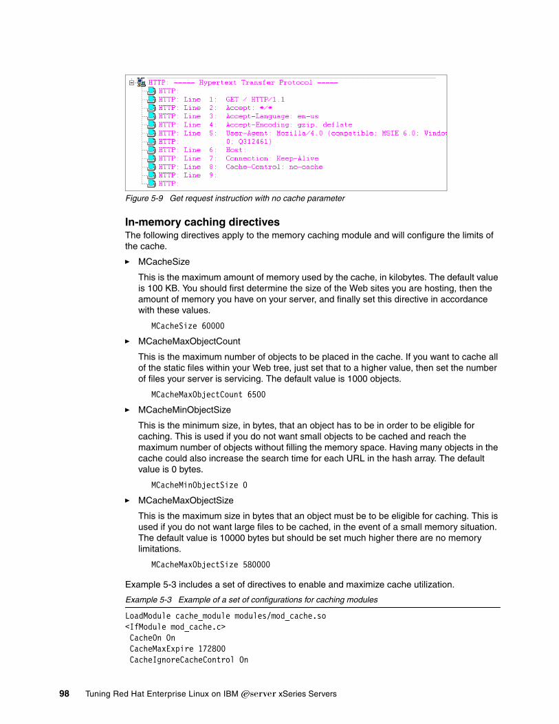
98 Tuning Red Hat Enterprise Linux on IBM Eserver xSeries Servers
Figure 5-9 Get request instruction with no cache parameter
In-memory caching directivesThe following directives apply to the memory caching module and will configure the limits of the cache.
� MCacheSize
This is the maximum amount of memory used by the cache, in kilobytes. The default value is 100 KB. You should first determine the size of the Web sites you are hosting, then the amount of memory you have on your server, and finally set this directive in accordance with these values.
MCacheSize 60000
� MCacheMaxObjectCount
This is the maximum number of objects to be placed in the cache. If you want to cache all of the static files within your Web tree, just set that to a higher value, then set the number of files your server is servicing. The default value is 1000 objects.
MCacheMaxObjectCount 6500
� MCacheMinObjectSize
This is the minimum size, in bytes, that an object has to be in order to be eligible for caching. This is used if you do not want small objects to be cached and reach the maximum number of objects without filling the memory space. Having many objects in the cache could also increase the search time for each URL in the hash array. The default value is 0 bytes.
MCacheMinObjectSize 0
� MCacheMaxObjectSize
This is the maximum size in bytes that an object must be to be eligible for caching. This is used if you do not want large files to be cached, in the event of a small memory situation. The default value is 10000 bytes but should be set much higher there are no memory limitations.
MCacheMaxObjectSize 580000
Example 5-3 includes a set of directives to enable and maximize cache utilization.
Example 5-3 Example of a set of configurations for caching modules
LoadModule cache_module modules/mod_cache.so <IfModule mod_cache.c> CacheOn On CacheMaxExpire 172800 CacheIgnoreCacheControl On

Chapter 5. Tuning Apache 99
LoadModule mem_cache_module modules/mod_mem_cache.so <IfModule mod_mem_cache.c> MCacheEnable mem / MCacheSize 65000 MCacheMaxObjectCount 6500 MCacheMinObjectSize 0 MCacheMaxObjectSize 580000 </IfModule> </IfModule>
Making sure a file is cachedHow can you tell whether your cache is working correctly? First, you should be able to measure a performance improvement. If you need to see details, you can change the logging level to debug and make at least two requests for the same file to your Apache Web server.
Example 5-4 displays the error log trace of two requests performed on the default Apache Web page (index.html, which includes apache_pg.gif). The first request services the two files from the disk and caches only the GIF file because the no-cache parameter was in the request and the CacheIgnoreCacheControl was not set to On. As you can see, the second request handles the GIF file from the cache.
You should also monitor your memory utilization; with caching on, it should increase.
Example 5-4 Caching modules logging
[debug] mod_cache.c(109): cache: URL / is being handled by mem[debug] mod_cache.c(109): cache: URL /index.html is being handled by mem[debug] mod_cache.c(109): cache: URL /index.html.var is being handled by mem[debug] mod_cache.c(109): cache: URL /apache_pb.gif is being handled by mem[debug] mod_cache.c(194): cache: no cache - add cache_in filter and DECLINE[debug] mod_cache.c(419): cache: running CACHE_IN filter[debug] mod_cache.c(650): cache: Caching url: /apache_pb.gif[debug] mod_cache.c(681): cache: Added date header[debug] mod_cache.c(109): cache: URL / is being handled by mem[debug] mod_cache.c(109): cache: URL /index.html is being handled by mem[debug] mod_cache.c(109): cache: URL /index.html.var is being handled by mem[debug] mod_cache.c(109): cache: URL /apache_pb.gif is being handled by mem[debug] mod_cache.c(211): cache: fresh cache - add cache_out filter and handle request[debug] mod_cache.c(339): cache: running CACHE_OUT filter[debug] mod_cache.c(351): cache: serving cached version of /apache_pb.gif
5.7 Monitoring ApacheApache 2.0 does not include graphical monitoring tools, but you can use the tools that are described in Chapter 2, “Monitoring tools” on page 15, to monitor your Web server activities.
For example, KDE System Guard gives you access to data on four subsystems: CPU, memory, network, and disk. You select the specific sensors you wish to monitor in the workspace area of KDE System Guard. Figure 5-10 on page 100 displays part of the sensors that are available to monitor your Apache server on Linux.
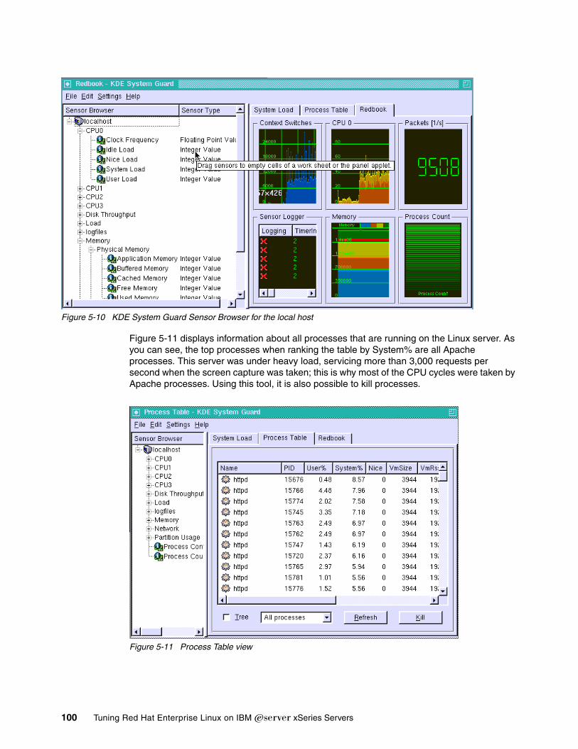
100 Tuning Red Hat Enterprise Linux on IBM Eserver xSeries Servers
Figure 5-10 KDE System Guard Sensor Browser for the local host
Figure 5-11 displays information about all processes that are running on the Linux server. As you can see, the top processes when ranking the table by System% are all Apache processes. This server was under heavy load, servicing more than 3,000 requests per second when the screen capture was taken; this is why most of the CPU cycles were taken by Apache processes. Using this tool, it is also possible to kill processes.
Figure 5-11 Process Table view

© Copyright IBM Corp. 2005. All rights reserved. 101
Chapter 6. Tuning database servers
The database server’s primary function is to search and retrieve data from disk. Database engines that are available on Linux currently include IBM DB2 and Oracle. Database servers require high CPU power and an efficient disk subsystem because they issue many random I/O requests. A large amount of memory is also important, because it involves CPU subsystems.
A balanced system is especially important. When you add a new CPU, you should consider upgrading other subsystems as well (for example, by adding more memory and improving disk resources).
In database servers, the design of an application, such as database and index, is critical.
This chapter covers the following topics:
� 6.1, “Important subsystems” on page 102� 6.2, “Optimizing the disk subsystem” on page 102� 6.3, “Optimizing DB2 memory usage” on page 104� 6.4, “Optimizing Oracle memory usage” on page 106
6

102 Tuning Red Hat Enterprise Linux on IBM Eserver xSeries Servers
6.1 Important subsystemsKey subsystems for databases are:
� Processors
CPU power is an important factor for database servers. Database queries and update operations require much CPU time. The database replication process also requires considerable numbers of CPU cycles.
Database servers are multithreaded applications, so SMP-capable systems provide better performance. Database applications scale very well, up to 16 processors and beyond. L2 cache size is also important because the hit ratio is high, approaching 90% in some cases.
� Memory
The amount of memory is a very important performance factor for database servers. Buffer caches are the most important part of a database server, so they require large amounts of memory to maintain data in the system memory. If the server does not have sufficient memory, disks will be accessed, which generates latencies.
Remember that system memory is also used for operating system needs. You should install enough memory for the OS to work properly; otherwise, paging is unavoidable.
When compiling the kernel, make sure that the CONFIG_HIGHMEM64G_HIGHPTE option has been set to y. This enables all of the memory to be used by the database processes, and the page tables can grow and map to high memory.
� Disk
Even with sufficient memory, most database servers will perform large amounts of disk I/O to bring data records into memory and flush modified data to disk. Therefore, it is important to configure sufficient numbers of disk drives to match the CPU processing power being used.
In general, a minimum of 10 high-speed disk drives is required for each Xeon processor. Optimal configurations can require more than 50 10K-RPM disk drives per Xeon CPU. With most database applications, more drives equals greater performance. For example, the xSeries 370 needs more than 450 10K RPM drives to reach maximum throughput when executing more than 40,000 transactions per minute.
6.2 Optimizing the disk subsystemThe main factors affecting performance include:
� The RAID controllers cache size� The choice of RAID levels for the various data sets� The RAID arrays stripe unit size� The database block size
6.2.1 RAID controllers cache sizeDepending on storage access patterns, the RAID controller cache may have a major impact on system performance. The cache plays a particularly relevant role for write operations on RAID 5 arrays. Write buffering makes the RAID controller acknowledge the write operation before the write goes to disk. This may positively affect performance in several ways:
� Updates can overwrite previous updates, thereby reducing the number of disk writes.
� By grouping several requests, the disk scheduler may achieve optimal performance.

Chapter 6. Tuning database servers 103
� By grouping sequential write requests in the controller cache, small writes (operations updating a single stripe unit) may be converted into large writes (full stripe write operations updating all the stripe units of a stripe).
However, the relevance of cache size should not be overestimated. The existence of a small cache may deliver high benefits, but often the marginal benefits of doubling the cache size are minimal. Moreover, remember that the RAID controller cache is only one of the many caches that affect I/O subsystem performance. A major role is played by the DBMS caches.
6.2.2 Optimal RAID levelDisregarding any cost constraint, the best choice is almost always RAID 10. The issue is to understand which activities merit the higher cost of the RAID 10 performance increase:
� In a data warehouse (DW), the typical access pattern to data files is almost 100% reading; therefore the better performance delivered by RAID 10 arrays in write operations is irrelevant and the choice of a RAID 5 level is acceptable.
� On the other hand, in a typical online transaction processing (OLTP) environment, the huge number of write operations makes RAID 10 the best level for data files arrays. Of course, even for the OLTP data files, RAID 5 may be acceptable in case of low concurrency.
For write operations, RAID 10 arrays are much better than RAID 5 arrays. However, for read operations, the difference between the two levels is minimal. From this simple rule stem the following recommendations:
� Online redo log files: RAID 1 is strongly recommended. In case of very high performance requirements, RAID 10 may be necessary. However, RAID 10 delivers performance benefits only in the case of quite small stripe unit size.
� Archive redo log files: RAID 1 is recommended. However, the archive redo logs are not as critical for performance as redo log files. Accordingly, it is better to have archive redo logs on RAID 5 arrays than to have redo logs on RAID 5 arrays.
� Temporary segments: RAID 1 (or, even better, RAID 10) is recommended in case of many sort operations, as is typical in data warehouses, for example.
� Data files: RAID 5 is acceptable for data warehouses, because the typical access pattern is reading for small databases. Generally, RAID 10 is the recommended RAID level.
6.2.3 Optimal stripe unit sizeTypically, the stripe unit size should be a multiple of the database block size (for example, two times or three times the block size).
In addition, consider the average I/O size. Theoretically, the I/O size and the stripe unit size should be identical. However, because block boundaries are not necessarily aligned with stripe units, you should make the stripe unit size at least twice the average I/O size.
6.2.4 Database block sizeThe database block size is one parameter that significantly affects I/O performance. However, the only way to change this parameter after the database is created is to create a new database and move data to it. The following general rules may help with decision making:
� The typical database block size for OLTP systems is 8 KB or 16 KB.
� The typical DB block size for data warehouse (DW) systems is 16 KB or 32 KB, and perhaps even 64 KB.

104 Tuning Red Hat Enterprise Linux on IBM Eserver xSeries Servers
In addition, the selected block size should be a multiple of the operating system basic block size (allocation unit), to avoid unnecessary I/O operations.
Oracle 9i supports multiple block sizes in the same database. This capability improves I/O performance because you can select the best block size for each table space in a database.
6.3 Optimizing DB2 memory usageThe way the Linux kernel manages physical memory is important to database server performance. On IA-32 architecture, the kernel manages memory in 4 KB pages. However, most modern processors are capable of working with larger pages (up to several megabytes).
For many applications, using 4 KB pages is suitable. Small pages reduce internal fragmentation, incur a smaller overhead when swapping data in and out of memory, and ensure that the virtual memory that is in use is resident in physical memory. Most database servers, however, use large shared memory segments for their database buffers. The result is that several page table entries (PTE) are required. This adds considerable maintenance overhead for the memory manager.
For example, consider a database server that allocates 1 GB of shared memory for its buffers using 4 MB shared memory segments. A kernel using 4 KB page size would require 262,144 PTEs, a significant number of page tables, which adds considerable maintenance overhead for the memory manager. However, note that this calculation is an oversimplification. The actual number of PTEs would be much larger because Linux cannot share page tables for shared memory.
On the other hand, the use of large pages can have a positive impact on database performance, especially for large database environments with many concurrent users. Large pages can reduce cache (table lookaside buffer, or TLB) misses. Also, they reduce the number of page table entries (PTEs), which reduces memory pressures on the system.
For example, suppose you have 1 GB of memory for buffer pools. The amount of memory required for the PTEs is 2 MB per agent. Assuming that you have 500 concurrent users, this works out to a total of 1 GB memory used for PTEs, which can be a very big waste for a Linux system. The use of large pages will reduce the number of required PTEs.
6.3.1 Buffer poolsProper memory utilization and data buffering is the key to database performance. At some point, all database activities require utilization of the various DB2 UDB buffer pools, caches, and heaps. The primary memory area is the buffer pool, which is the work area for DB2 data pages. A data page is the allocation unit where rows of table data or index data are stored. The purpose of the buffer pool is to improve system performance. Data can be accessed much faster from memory than from disk; therefore, the fewer times the database manager has to read from or write to a disk (I/O), the better the performance.
Key ideas for effective buffer pool utilization are:
� The larger the buffer pool, the more data can be stored.� Keep more frequently accessed data in the buffer pool.� Keep essential index data in the buffer pool for faster data access.
To accomplish these goals, changes to the size and number of buffer pools may be required. This can be accomplished manually or by using the DB2 UDB performance wizard.

Chapter 6. Tuning database servers 105
With DB2, you can segment your data into different categories by creating separate table spaces for disparate data (frequently accessed data, history, index, sequentially accessed data, randomly accessed data, index data, LOB data). By segmenting the data, you can assign different buffer pools to corresponding table spaces, thereby controlling the data and system memory utilization.
A primary goal of performance tuning should be to minimize disk I/O. If I/O is necessary, it is important to make it as efficient as possible. There are two effective ideas for efficient I/O:
� Prefetching: The concept of moving data into the buffer pool before it is required by the application. When to perform prefetching is largely a function of the database engine being able to either determine that prefetching data will be beneficial or, as a query is performed, detect that prefetching will be helpful.
� Parallel I/O: Moving data more quickly into the buffer pool by performing I/O operations simultaneously rather than sequentially. There are several ways to affect the amount of parallel I/O. The overall principle is to try to spread data access across as many physical drives as possible.
RAID devices perform this task at a lower layer than the database engine. DB2 UDB can perform parallel I/O on a single RAID volume or across RAID volumes. If data is placed on a single RAID volume (for example, drive D:), the database engine does not know that the device is capable of performing multiple I/O operations simultaneously.
The DB2_PARALLEL_IO parameter is used to inform the database engine that volumes are available for parallel I/O operations. To set this variable, open a DB2 command window and enter:
DB2SET DB2_PARALLEL_IO=*
This turns on parallel I/O for all volumes. This usually is a good idea when using hardware RAID devices. If database data is placed on multiple RAID volumes, it is automatically available for parallelism.
6.3.2 Table spacesData storage in DB2 UDB is based on the concept of table spaces. A table space is created from one or more containers. Containers are the locations for data placement and can be directories, specific files, or entire volumes.
There are two types of table spaces:
� System Managed Space (SMS)
SMS table spaces are the simplest to administer. They contain one container, which is a directory where DB2 UDB creates and manipulates data files as needed and which is limited only by the size of the volume where the directory lives. This type of table space cannot send table and index data pages into separate buffer pools. Also, data pages may not be contiguous because the OS has greater control over physical placement of data on the volume.
� Database Managed Space (DMS)
DMS table spaces have greater control over data placement. The containers for a DMS table space are either files of a specified size or entire raw volumes. Using file containers, there should only be one file per volume and each container should be of the same size. As DMS table space containers fill up, you may either increase the size of the containers if the containing volumes have available space or add containers to the table space.
The DMS table space type allows for table and index data to be separated into different table spaces, thereby separating buffer pools. DMS data is also more likely to be stored contiguously, making for more efficient I/O.

106 Tuning Red Hat Enterprise Linux on IBM Eserver xSeries Servers
The database configuration parameter NUM_IOSERVERS specifies how many database agents are available for performing prefetching and parallel I/O operations. This should be set to one or two more than the number of physical drives that make up the volumes where DB2 data is stored.
Another important I/O operation is logging. All database data changes must be logged in order to guarantee data consistency, so it is important that the logging activity does not become a bottleneck. DB2 UDB database logs should be placed on a volume with enough physical drives to meet the write-intensive work of the logger. The database configuration parameter NEWLOGPATH is used to specify the path where the database logs are created.
6.4 Optimizing Oracle memory usageThis section describes tuning activities related to Oracle and the use of memory.
Oracle instance memory tuning is one of the areas where small parameter changes can produce a big increase, as well as a big decrease, of performance. In this section, we describe the shared pool, database buffer tuning, and redo log buffer.
6.4.1 Shared poolThe shared pool consists of two areas: the library cache and the dictionary cache.
� Library cache
The library cache includes three memory areas:
– Shared SQL area: contains the execution plans of parsed SQL statements– PL/SQL programs: contains PL/SQL programs in compiled forms– Locks
Oracle dynamically tunes the relative size of these areas. The only manually tunable parameter is the shared pool global size variable SHARED_POOL_SIZE. To see whether the library cache is properly sized, the following simple SQL instruction can be used:
select round((sum(pins-reloads)/sum(pins))*100,2) as hit_ratiofrom v$librarycache;
The term pins refers to the number of times a parsed SQL statement was looked for in the library cache. The reloads are the number of times the search was unsuccessful. The library cache hit ratio should be as high as 99%. If the hit ratio is lower, either the instance has been recently started, so the cache is suboptimal, or the shared pool is insufficient and the size should be made larger.
� Dictionary cache
This simple SQL instruction shows whether the size of the dictionary cache is optimal:
select round((sum(gets-getmisses)/sum(gets))*100,2) as hit_ratiofrom v$rowcache;
The term gets refers to the number of times a request was made for information in the dictionary cache, while the term getmisses refers to the number of unsuccessful requests. The dictionary cache hit ratio should be as high as 99%. If the hit ratio is lower, either the instance has been recently started, so the cache is suboptimal, or the shared pool is insufficient and the size should be made larger.

Chapter 6. Tuning database servers 107
6.4.2 Database buffer cacheServer foreground processes read from data files into the database buffer cache, so the next readings need no I/O operation. Server processes also write modified data into the database buffer cache. Asynchronously, a dedicated background process (DBWn) moves dirty data from the cache to the data files, and this greatly increases I/O performance. The performance benefits obviously depend on cache hits (that is, how many times server processes looking for data find them in the cache). This section describes the internal structure of the buffer cache and how to tune it.
Buffer cache architectureThe buffer cache consists of as many buffers as the value of the init<sid>.ora parameter DB_BLOCK_BUFFERS. The sizes of the buffers are identical and correspond to the init<sid>.ora parameter DB_BLOCK_SIZE. The buffer cache is filled in by foreground processes reading data from data files and flushed out by the DBWn process when one of the following events occurs:
� DBWn time-out (each three seconds)� Checkpoint� No free buffer
Data is removed from the buffer cache according to the least recently used algorithm. To avoid cache quality worsening due to single full-table scan instructions, Table Access Full operations are always put at the end of LRU lists.
Optimal buffer cacheTo see whether the size of the buffer cache is optimal, the following query can be used:
select name, valuefrom v$sysstatwhere name in (‘db block gets’, ‘consistent gets’, ‘physical reads’);
Given the output of this select command, the buffer cache hit ratio can be obtained with the following simple calculation:
Enlarging the buffer cacheThe buffer cache hit-ratio should be 90% or higher. Values between 70% and 90% are acceptable if it is necessary to resize the buffer cache to improve the library or dictionary hit cache ratios. If the buffer cache hit ratio is too low, the optimal number of buffers to add to the cache can be obtained with this complex query on the V$DB_CACHE_ADVICE view:
column size_for_estimate format 999,999,999,999 heading ’Cache Size (m)’column buffers_for_estimate format 999,999,999 heading ’Buffers’column estd_physical_read_factor format 999.90 heading ’Estd Phys|Read Factor’column estd_physical_reads format 999,999,999 heading ’Estd Phys| Reads’
SELECT size_for_estimate, buffers_for_estimate, estd_physical_read_factor, estd_physical_readsFROM V$DB_CACHE_ADVICEWHERE name = ’DEFAULT’AND block_size = (SELECT value FROM V$PARAMETER
WHERE name = ’db_block_size’)AND advice_status = ’ON’;
dbblockgets consistentgets physicalreads–+dbblockgets consistentgets+( )
------------------------------------------------------------------------------------------------------------------------------------ 100×

108 Tuning Red Hat Enterprise Linux on IBM Eserver xSeries Servers
Before running the query, the V$DB_CACHE_ADVICE view has to be activated by using the following command:
alter system set DB_CACHE_ADVICE=ON;
To obtain significant results, a representative workload should have been running on the system for a reasonable time interval, thereby achieving a stable buffer population.
Because the activation of the V$DB_CACHE_ADVICE view has a (minor) impact on CPU load and memory allocation, at the end of the analysis, de-activating the view with this command is recommended:
alter system set DB_CACHE_ADVICE=OFF;
The output of the query is a set of lines showing the incremental benefits of the various cache sizes. The first column of the query output contains the various cache sizes while the latter column shows the physical reads. Upon increasing the cache size, the physical reads decrease, but the incremental benefits also decrease.
Multiple buffer poolsStarting with Oracle 8, multiple buffer pools can be created and separately sized. The database buffer cache consists of these three buffer pools:
� Keep pool� Recycle pool� Default pool
The keep pool stores data that must not be moved out of the buffer cache. The recycle pool is for data that must be moved quickly out of the buffer cache when no longer necessary. Everything else is in the default pool. Unlike the shared pool, whose internal memory areas (library cache, dictionary cache) cannot be sized separately, it is possible to size the keep pool and the recycle pool, and also, as a result, the default pool.
The following example shows how to size a 1000-buffers buffer cache so that 50% is used for the recycle pool, 25% for the keep pool, and 25% for the default pool:
DB_BLOCK_BUFFERS=1000DB_BLOCK_LRU_LATCHES=20BUFFER_POOL_RECYCLE=(buffers:500, lru_latches:10)BUFFER_POOL_KEEP=(buffers:250, lru_latches:5)
Latches are memory locks, and they should be sized at the rate of one latch for each 50 buffers, as in the example above.
6.4.3 Redo log buffer cacheEach server process that updates data has to update the redo log files first. To improve performance, server processes only write redo log entries into the redo log buffer cache, and the LGWR process is responsible for moving dirty buffers from memory to disks. To avoid buffer data corruption, a locking mechanism (latch) is used, so that only one process at a time can write on the redo log buffer cache. Given the sequential nature of redo log data, only one redo log allocation latch is made available to Oracle server processes. As a result, redo log buffers can be a source of delay because of high resource contention.
To see whether there is an excessive redo log buffer contention, use this query:
select name, valuefrom v$sysstatwhere name=’redo buffer allocation retries’;

Chapter 6. Tuning database servers 109
Any value other than 0 shows that processes had to wait for space in the redo log buffer cache.
The size of the redo log buffer can be configured by changing the LOG_BUFFER parameter in the init<sid>.ora file. This parameter gives the value in bytes of the cache and must be a multiple of DB_BLOCK_SIZE.
Each server process wanting to write to the redo log buffer cache must first get the redo allocation latch. The process then writes as many bytes as allowed by the LOG_SMALL_ENTRY_MAX_SIZE parameter in init<sid>.ora. When this number of bytes has been written, the process must release the latch in order to allow other processes to have a chance to acquire the lock. To increase the ability of server processes to work concurrently, you should size the LOG_SMALL_ENTRY_MAX_SIZE parameter as small as possible.

110 Tuning Red Hat Enterprise Linux on IBM Eserver xSeries Servers

© Copyright IBM Corp. 2005. All rights reserved. 111
Chapter 7. Tuning LDAP
Lightweight Directory Access Protocol (LDAP) is a technology for accessing common directory information. LDAP has been embraced and implemented in most network-oriented middleware. As an open, vendor-neutral standard, LDAP provides an extendable architecture for centralized storage and management of information that must be available for today’s distributed systems and services. LDAP has become the de facto access method for directory information, much as DNS is used for IP address look-up on the Internet.
For example, LDAP can be used to centralize logon information for all systems on your network. This replaces the need to maintain that information on each system (normally stored in /etc/passwd and /etc/shadow). An LDAP object for a user may contain this information:
dn: uid=erica,ou=staff,dc=redpaper,dc=comcn: Erica Santimuid: esantimuidNumber: 1001gidNumber: 100homeDirectory: /export/home/esantimloginShell: /bin/kshobjectClass: topobjectClass: posixAccount
These objects are identified by the DN (name) attribute that works like a primary key in any database.
This chapter includes the following topics:
� 7.1, “Hardware subsystems” on page 112� 7.2, “Operating system optimizations” on page 112� 7.3, “OpenLDAP 2 optimizations” on page 112
For details about LDAP implementation and optimization, see the IBM Redbook Understanding LDAP - Design and Implementation, SG24-4986.
7

112 Tuning Red Hat Enterprise Linux on IBM Eserver xSeries Servers
7.1 Hardware subsystemsAn LDAP directory is often described as a database, but it is a specialized database with characteristics that set it apart from general purpose relational databases. One special characteristic of directories is that they are accessed (read or searched) much more often than they are updated (written). Hundreds of people might look up an individual’s phone number, or thousands of print clients might look up the characteristics of a particular printer. But the phone number or printer characteristics rarely change. LDAP directories are typically optimized for read access.
Key hardware subsystems are:
� Swap and physical memory� CPU utilization and I/O in disks
Consider the following recommendations:
� Memory is often the bottleneck for LDAP servers. Ensure that your server has enough installed.
� Separate the LDAP directories and the logs onto separate disks or RAID arrays.
� The LDAP server daemon slapd uses memory and CPU to perform indexing in order to improve look-up times. Cache usage is controlled by settings in slapd.conf.
7.2 Operating system optimizationsWe can manage our server’s performance by limiting the amount of resources the server uses to process client search requests. The following parameters can be altered. Ongoing monitoring of the system is important.
� The time during which the server maintains the FIN-WAIT-2 connections before terminating them is controlled by tcp_fin_timeout:
sysctl -w net.ipv4.tcp_fin_timeout=15
� The maximum number of file descriptors that Linux can have open at any one time is specified by file-max:
sysctl -w fs.file-max=131063
� Disable the writing of access time stamps to files to increase I/O performance by adding the noatime parameter to /etc/fstab as follows:
LABEL=/ / ext3 defaults,noatime 1 1
� Enable asynchronous I/O so that a process does not have to wait for the I/O response to be ready:
LABEL=/ / ext3 defaults,noatime,async 1 1
7.3 OpenLDAP 2 optimizationsHere are some tuning parameters that may improve performance of your OpenLDAP installation. Make these changes in the /etc/openldap/slapd.conf file:
� idletimeout specifies how long the LDAP server should wait (in seconds) before closing an idle client connection. The default is 0 (disable), but two minutes is enough:
idletimeout 120

Chapter 7. Tuning LDAP 113
� Limit the maximum number of entries that can be returned from a search operation. This is especially important when clients uses wild cards on searches. The default is 500.
sizelimit 100
� Specify the maximum number, in seconds, that OpenLDAP spends answering a client request. The default is 3600 (60 minutes). Normally, you can reduce this to 10 minutes.
timelimit 360
� Disable all logging unless you need the information:
loglevel 0
7.3.1 Indexing objectsIndexing LDAP objects ensures that searches on those objects are quicker and consume fewer server resources. However, indexing objects that are rarely or not used for searches also affects performance.
OpenLDAP enables you to specify what objects will be indexed using the index statements in the slapd.conf file:
index {<attrlist> | default} [eq,sub,pres,approx,none]
attrlist specifies which attributes to index. The second parameter specifies what type of index is created:
� eq means equality: an exact match. For example, cn=optical only returns results where cn is exactly the string optical. eq implies pres, so adding pres is unnecessary.
� sub means substring: for example, cn=*optical* returns all values of cn containing the string optical.
� pres means presence: if the attribute is present in an entry.
� approx means approximate: where the value sounds like the search result. This is based on the enable-phonetic compile parameter.
� none means not indexed.
For example:
index cnindex sn,uid eq,subindex default none
The first line specifies that the LDAP will index attribute cn for all kinds of available searches. The second line specifies that attributes sn and uid will be indexed only when the search includes eq and sub. The third line specifies that no other attributes will be indexed.
By default, no indexes are maintained. It is generally advised that at a minimum, an equality index of objectClass be maintained.
Tip: Do not use idletimeout with the tcp_tw_reuse kernel parameter because LDAP drops reused connections. If you need to solve problems with excessive TCP connections, we recommend that you disable idletimeout and configure tcp_tw_reuse and tcp_tw_recycle.

114 Tuning Red Hat Enterprise Linux on IBM Eserver xSeries Servers
7.3.2 CachingFrequent searches will benefit from the use of cache. This portion of memory stores the data that is used to determine the results, thereby making common searches much faster.
To specify the amount of memory used for the cache associated with each open index file, use the dbcachesize parameter, in bytes. The default is 100000:
dbcachesize 100000
You can also specify how many attributes of the most frequent searches OpenLDAP will put in memory. The default is 1000 entries:
cachesize 1000

© Copyright IBM Corp. 2005. All rights reserved. 115
Chapter 8. Tuning Lotus Domino
Lotus® Domino® is a popular application and messaging system that enables a broad range of secure, interactive business solutions for the Internet and intranets. The Lotus Domino server is a powerful tool for organizational communication, collaboration, and information sharing.
Just as for other application servers, careful planning, maintenance, and tuning processes are essential in systems administration. This chapter discusses the tuning concepts and procedures of Lotus Domino R6.5 server running on Linux.
Topics covered are:
� 8.1, “Important subsystems” on page 116� 8.2, “Optimizing the operating system” on page 118� 8.3, “Domino tuning” on page 119
The chapter is based, in part, on the Redpaper Domino for IBM Eserver xSeries and BladeCenter Sizing and Performance Tuning, REDP3851, which is available from:
http://www.redbooks.ibm.com/abstracts/redp3851.html
8

116 Tuning Red Hat Enterprise Linux on IBM Eserver xSeries Servers
8.1 Important subsystemsLotus Domino server can act as a mail, Web, application, hub, and database server, handling mail routing and storage as well as database and Web requests. Because of the dynamic nature of Lotus Domino, the important subsystems that can be sources of a bottleneck are:
� Network� Memory� CPU� Disk
Refer to Chapter 4, “Analyzing performance bottlenecks” on page 69 for more information about detecting and removing bottlenecks related to these subsystems.
As you identify which subsystems are potential sources of bottlenecks, you will have a general idea of what initial actions to take regarding performance optimization.
8.1.1 Network adapter cardWhen analyzing network performance and potential bottlenecks, the following parameters should be investigated to maximize performance:
� Network adapters� Ethernet adapter performance� TCP/IP performance� Operating system settings� Network design
Network compression is a performance feature of Domino 6.5. When you enable network compression, data is compressed automatically before it is sent over the network. This improves network performance, especially over slower line speeds. Network compression can result in 34% to 52% less network traffic and enable faster message delivery.
We recommend the following network adapter configuration for your server, especially if your Domino system is utilized by a large number of users:
� Use the onboard Ethernet adapter (10/100/1000 Mbps) in the server where possible.
� A Gigabit Ethernet connection from the server to the Ethernet switch is recommended.
� Use an IBM PCI-X Ethernet adapter with full-duplex capability.
� For servers that will support a large number of users, consider using multiple network adapters.
8.1.2 Server memoryThe minimum amount of RAM your Domino server requires depends on two primary factors. Domino and the operating system (OS) need a base amount of RAM to be able to execute on the hardware; this is the first component of the total RAM required. The second component depends on how many Notes and Web clients have sessions with your server and on what
Tip: Never assume that you do not have a LAN bottleneck simply by looking at LAN sustained throughput in bytes/sec. LAN adapter bottlenecks often occur at low LAN utilization but high sustained packet rates. Observing packets/sec often yields clues about these types of bottlenecks.

Chapter 8. Tuning Lotus Domino 117
other tasks your server might have to perform. The memory model has been redesigned in Domino 6.5, and this has meant a 30% reduction in memory requirements per user.
Use this formula to calculate the minimum amount of RAM your Domino 6.5 server requires:
Remember that this RAM requirement includes only the OS and Domino running on your server. Any file and print services, backup and recovery, or anti-virus software running on your server requires additional RAM. For example, if the calculation above determines that you need 158 MB of RAM, install 256 MB.
This algorithm is appropriate for mail and application servers and mail hubs. However, it is not appropriate for replication hubs. Usually, replication hubs are heavily used but have few, if any, sessions open to active users.
Total memory minus available memory equals the amount of memory the server is actually using, sometimes called the working set. Because memory use is dynamic, it is best to monitor memory utilization over an extended period of time to arrive at an accurate representation of the memory working set. To determine the amount of memory needed to support double the users, double the working set size and add 30% as a buffer for peak activity.
Servers should be configured so that average memory utilization does not exceed 70%. If this level is exceeded consistently, you run the risk that the server will expand storage onto disk (page memory onto disk) during periods of peak activity. Servers should never regularly page memory to disk, because this adversely affects performance.
8.1.3 ProcessorsDomino 6.5 reduces the CPU requirement per user by as much as 23%, enabling servers to handle more users.
Many Domino functions are processor-intensive. Tasks such as routing messages, indexing databases, searching databases, and dynamically creating HTML pages for Web clients all put heavy demands on the system’s CPU, so we recommend that you purchase an xSeries server that supports at least two-way SMP. You might not need or be able to afford the extra CPUs today, but this provides room to grow as use of Domino functions expands.
Domino can take advantage of the benefits of SMP. It does so automatically; you do not need to tune or configure your hardware for Domino to take advantage of the additional CPUs. Domino takes advantage of multiple processors by allocating the replicator and router tasks to different CPUs, thereby spreading the load.
Minimum memory requirements: 128 MB + (number of concurrent users/5) MB
Note: Lotus Domino only addresses up to 2 GB of RAM. If you install extra memory, it will be used only by the OS and other additional tasks. This means that installing more than 2.5 GB of RAM will not significantly improve server performance.
Memory guideline: Paging I/O should occur only occasionally, such as when applications are initializing, but never on a continuous basis. Average memory utilization should not exceed 70% of available memory.

118 Tuning Red Hat Enterprise Linux on IBM Eserver xSeries Servers
8.1.4 Disk controllersSeveral xSeries servers have redundant array of independent disks (RAID) technology as their standard. This enables data to be striped across a number of hard disks that are seen by the OS as one large disk drive.
For your Domino server, we recommend:
� Implement RAID-1E or RAID-10 on all of your servers if financially possible, or RAID-5 or RAID-50 as a second choice. As your Domino servers become more critical to your business, you will want the best combination of disk fault tolerance and performance you can afford.
� Implement a second RAID-1E array to store the Domino 6 transaction logs.
� Do not implement multiple logical drives or partitions on the same RAID array. For each RAID array, create only one logical drive, and on that logical drive, only one partition. This will reduce latency due to extreme drive head movement.
� Only use hardware-controlled RAID arrays. Software-controlled RAID arrays place additional strain on your server in terms of CPU utilization. The CPU should be dedicated to providing Domino functions, not implementing a RAID subsystem.
� If possible, install an additional hard disk for use as a hot spare. Hot spares can replace failed disks automatically, or can be managed by the administrator.
� Choose the fastest hard drives. High-performance disks provide fast data rates and low latency times. xSeries servers support very fast 15,000 RPM drives.
� Do not mix SCSI Fast with SCSI Fast/Wide drives.
� Do not mix drives that spin at different speeds.
� Do not mix drives of different sizes in a RAID array.
� Enable write-back cache on the RAID controller. This setting improves system performance by caching information before it is written back to disk. Some controllers do not have battery backups, and cached data will be lost in the event of a power failure. In this situation, installing an uninterruptible power supply (UPS) for your server is particularly important.
� Set the RAID stripe size to 16 KB.
� Install the latest BIOS, firmware, and drivers for the disk controller (ServeRAID or Fibre Channel, for example).
8.2 Optimizing the operating systemSeveral kernel parameters can affect Domino server performance. For more about tuning these parameters, refer to Chapter 3, “Tuning the operating system” on page 35.
� fs.file-max
This specifies the maximum number of file handles that can be opened by Domino. The command sysctl fs.file-max shows the current value. Ensure that the value is at least 49152 (48 x 1024). You may find the default value to be higher than this value; in that case, leave it unchanged.
sysctl -w fs.file-max=49152
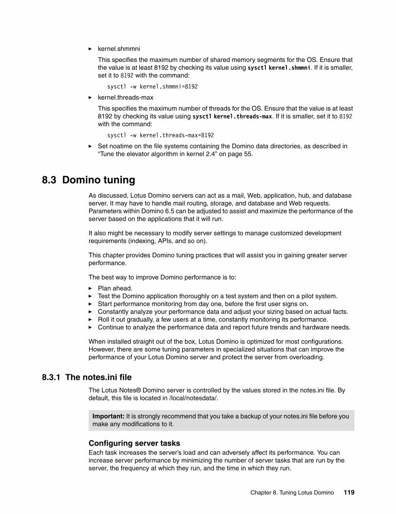
Chapter 8. Tuning Lotus Domino 119
� kernel.shmmni
This specifies the maximum number of shared memory segments for the OS. Ensure that the value is at least 8192 by checking its value using sysctl kernel.shmmni. If it is smaller, set it to 8192 with the command:
sysctl -w kernel.shmmni=8192
� kernel.threads-max
This specifies the maximum number of threads for the OS. Ensure that the value is at least 8192 by checking its value using sysctl kernel.threads-max. If it is smaller, set it to 8192 with the command:
sysctl -w kernel.threads-max=8192
� Set noatime on the file systems containing the Domino data directories, as described in “Tune the elevator algorithm in kernel 2.4” on page 55.
8.3 Domino tuningAs discussed, Lotus Domino servers can act as a mail, Web, application, hub, and database server. It may have to handle mail routing, storage, and database and Web requests. Parameters within Domino 6.5 can be adjusted to assist and maximize the performance of the server based on the applications that it will run.
It also might be necessary to modify server settings to manage customized development requirements (indexing, APIs, and so on).
This chapter provides Domino tuning practices that will assist you in gaining greater server performance.
The best way to improve Domino performance is to:
� Plan ahead.� Test the Domino application thoroughly on a test system and then on a pilot system.� Start performance monitoring from day one, before the first user signs on.� Constantly analyze your performance data and adjust your sizing based on actual facts.� Roll it out gradually, a few users at a time, constantly monitoring its performance.� Continue to analyze the performance data and report future trends and hardware needs.
When installed straight out of the box, Lotus Domino is optimized for most configurations. However, there are some tuning parameters in specialized situations that can improve the performance of your Lotus Domino server and protect the server from overloading.
8.3.1 The notes.ini file The Lotus Notes® Domino server is controlled by the values stored in the notes.ini file. By default, this file is located in /local/notesdata/.
Configuring server tasksEach task increases the server’s load and can adversely affect its performance. You can increase server performance by minimizing the number of server tasks that are run by the server, the frequency at which they run, and the time in which they run.
Important: It is strongly recommend that you take a backup of your notes.ini file before you make any modifications to it.

120 Tuning Red Hat Enterprise Linux on IBM Eserver xSeries Servers
Example 8-1 notes.ini servertasks list
ServerTasks=Update,Replica,Router,AMgr,AdminP,CalConn,SchedServerTasksAt1=Catalog,DesignServerTasksAt2=UpdAllServerTasksAt3=Object Info -FullServerTasksAt5=Statlog
Each of these variables controls the schedule for automatic server and database maintenance tasks. In Example 8-1, the first ServerTasks line denotes the services that are run when the Domino task starts while the other lines denote the scheduled server tasks. The time is entered in a 24-hour format, where 0 is 12:00 a.m. and 23 is 11:00 p.m. In the example above, Catalog and Design tasks start at 1:00 a.m., and the Statlog task starts at 5:00 a.m.
You can significantly improve performance by removing tasks that are not appropriate to the server. Consider the following suggestions to increase performance related to Lotus Domino server tasks.
� These tasks should be turned off when they are not in use:
– Scheduling: Turn off this task if you are not using the server for scheduling and calendaring.
– AMgr: Turn off this task if you are not using the server to run scheduled agents. Remember, this function is not required for WebQuery Agents.
– Collector, Reporter: Turn off this task if you are not using the server to automatically track server statistics on a regular basis. You can collect them on demand.
� Remove the Replicator (Replica) and Router tasks.
Both of these tasks can be removed if they are not being used on the server, because each takes up a fair amount of server resources when loaded. For example, if you have only one Lotus Domino server in your organization that is used for both applications and mail routing, you might not need the Replicator task, because you do not have any other servers from which to replicate (and because clients will be replicating from the Lotus Domino server, not vice versa).
� Carefully choose the times when server tasks are run.
Daily server tasks should not be run when other server tasks are running or at times when there are many users using the Lotus Domino server. This allows the maximum amount of server resources to be available for each server task that is currently executing and for user sessions. Examples of such server tasks are Design, Catalog, Statlog, and customized Notes API programs that have to be run only once a day.
The entries in ServerTasks have the following uses:
� ADMINP: The major Domino scheduler job running batch-like updates� AMGR: Domino Agent Manager; takes care of predefined agents� CALCONN: Connects the Domino calendar to other types of calendars� EVENT: Domino Event Handler� REPLICA: Domino database Replicator task� REPORT: Domino Report Generator (adds data to STATREP.NSF)� ROUTER: Domino Mail Routing task� SCHED: Domino Scheduler task� SERVER: The main Domino Server task� UPDATE: Updates the database indexes and views

Chapter 8. Tuning Lotus Domino 121
Domino database indexing: controlling the Update taskThe Update task is designed to run in the background and is intended to improve response time and performance by ensuring that when a user opens a database view, he or she does not have to wait for it to be indexed.
To improve view-indexing performance, you can run multiple Update tasks if your server has adequate CPU power. Doing this can affect server performance and is recommended primarily for multiprocessor machines. On a server with multiple processors, enable a maximum of one Update task per processor.
This is done in the notes.ini file by adding the line:
Updaters = [number of processors]
Network performance (compression)Network compression is an important performance feature offered in Lotus Notes/Domino 6. When you enable network compression, data is automatically compressed before it is sent over the network. This improves network performance, especially over slower lines.
Notes/Domino 6 network compression offers several immediate benefits. For example, by reducing the amount of data being transmitted, you can improve the performance of your routing and replicating hub servers, especially if they are currently laboring under heavy workloads. In addition, you can enable network compression by default, so all of your users can take advantage of this functionality without having to select it themselves. Because network compression is a standard, out-of-the-box feature, it does not require any additional code, which helps simplify administration and requires fewer CPU resources to run.
Note the following statistics about the benefits of network compression:
� A 35-52% reduction in data transferred from server to client� A 26% reduction in data transferred from server to server
Modify the TCP/IP line in the notes.ini file to enable network compression. The last parameter denotes compression:
TCPIP = TCP,0,15,0,,12320
Setting maximum mail threads for local deliveryThe MailMaxDeliveryThreads setting determines the maximum number of threads the router can create to perform local mail delivery. The default number is 1. Increasing this value can improve message throughput for local deliveries. The ideal number usually falls between 3 to 25, depending on the number of local deliveries on your Lotus Domino mail server.
MailMaxDeliveryThreads = [number]
Tip: An obvious but important lesson about server tasks and functions is that if your organizational requirements have no need for a function, you should not run it on your server!
Important: Do not remove the Update task from a server. If you do so, the Public Address Book will not be updated.

122 Tuning Red Hat Enterprise Linux on IBM Eserver xSeries Servers
Disabling per-user message caching by the IMAP taskThis setting disables per-user message caching by the IMAP task. It can improve the capacity of a server by reducing memory consumption. However, the response time for some user operations might be slower. If this setting is omitted, IMAP per-user message caching will be enabled.
To disable per-user message caching by the IMAP task, set the following value to 1:
NoMsgCache = [0 or 1]
Using the Lotus Domino 6.5 database formatDatabases that you create in Lotus Domino 6.5 perform considerably better than databases created in previous releases. Database operations require less I/O and fewer CPU resources, view rebuilding and updating are quicker, and memory and disk space allocation is improved.
Because of these performance improvements, limiting the size of the databases to improve database performance is less important than in past releases. The maximum database size for Lotus Domino 6.5 format databases is 64 GB.
Defining the number of databases cached simultaneouslyIf your server has sufficient memory, you can improve its performance by increasing the number of databases that Lotus Domino can cache in memory at one time. To do so, use the NSF_DbCache_Maxentries statement in the NOTES.INI file. The default value is 25 or the NSF_Buffer_Pool_Size divided by 300 KB, whichever value is greater. The maximum number of databases that can be cached in memory is approximately 10,000. For short intervals, Lotus Domino will store up to one and a half times the number entered for this variable.
Monitor the Database.DbCache.Hits statistic on your server. This indicates the number of times a database open request was satisfied by finding the database in cache. A high value indicates that the database cache is working effectively. If the ratio of Database.DbCache.Hits to InitialDbOpen is low, you might consider increasing NSF_DbCache_Maxentries.
To set the number of databases that a server can hold in its database cache at one time, set the NOTES.INI value as follows:
NSF_DbCache_Maxentries = [number]
In special circumstances, you might also want to disable the database caching. The database cache is enabled by default. To disable database caching, enter the following syntax on the Domino console:
Dbcache disable
The database cache keeps databases open. Use this command to disable the database cache when you need exclusive access to a file that might be in it. For example, to run an application such as a virus checker or backup software, disable the cache. To re-enable the database cache, restart the server.
Optimizing database index updateIn general, the fewer view indexes that the Indexer server task must update, the fewer server resources this task uses. You can use the NOTES.INI variable Default_Index_Lifetime_Days to minimize the amount of effort required by the Indexer task when updating view indexes. The Default_Index_Lifetime_Days variable controls how long a view index is kept in a database before it is deleted due to non-use:
Default_Index_Lifetime_Days = [number of days]

Chapter 8. Tuning Lotus Domino 123
Full-text indexesDisable the updating of full-text indexes on a server if you do not have any full-text indexed databases on your server (and do not intend to have any). The NOTES.INI variable Update_No_Fulltext can be used to disable all full-text index updating on the server. You might want to use this variable to disable the updating of full-text indexes if, for example, you do not want users to create full-text indexes of their mail files on a mail server in order to save disk space on that server and save the Indexer task the time and resources needed to update these full-text indexes. This is a very good setting for mail and replication hub servers, which in most circumstances do not have any user connections. The full-text index variable is:
Update_No_Fulltext = [0 or 1]
Setting this value to 0 causes full-text indexes to be updated each time the Update task (a server command task) is executed, and setting the value to 1 disables all full-text indexing.
Maximum sessions When a new user attempts to log on, if the current number of sessions is greater than the value of Server_MaxSessions (in the NOTES.INI file), the Lotus Domino server closes the least recently used session. For a session to be considered for closing, it must have been inactive for at least one minute. For example, if this parameter is set to 100, and the 101st person tries to access the Lotus Domino server, the Lotus Domino server drops the least-used session from the server in favor of this new session.
Controlling minimum mail poll timeYou can control the minimum allowable time in which Lotus Notes clients can poll for new mail. It is possible that your Lotus Domino server resources are being overtaxed by being constantly bombarded by requests for new mail from the Notes client machines if users have changed their default new mail notification check time from 15 minutes to a smaller number such as 2 or 5.
You can control the minimum frequency of these requests from the server by using the MinNewMailPoll NOTES.INI variable. This variable determines the minimum allowable checking time from clients regardless of the value specified on the client machines. No default is set during server setup. The syntax of this variable is:
MinNewMailPoll = [minutes]
Setting up multiple replication tasksYou can improve server replication performance by running multiple replicator tasks simultaneously. By default, only one replicator task is executed. With a single replicator task running, if you want to replicate with multiple servers at the same time, the first replication must complete before the next one can start. Set the number of replicators by adding the following entry in the NOTES.INI file, where the value is the number of replicators:
Replicators = [number]
All other factors aside, it is recommended that you set the number of replicator tasks equal to the number of spoke servers with which the hub replicates. However, to avoid putting too much load on the server you should not exceed 20 replicators. If the server you intended to
Reducing maximum server sessions: Reducing the Server_MaxSessions value to a specific number will not prevent the server from allowing more than that number of concurrent active users on the server, but will drop the sessions soon after they become inactive. This frees up resources. Conversely, Domino will not close any session that has been idle for less than one minute regardless of the demand on the server.

124 Tuning Red Hat Enterprise Linux on IBM Eserver xSeries Servers
replicate is not a hub server, the recommended number of replicators should equal the number of processors on the server.
8.3.2 Enabling transaction loggingTransaction logging is available in Lotus Domino 6.5 servers. With transaction logging, each transaction is transferred to its database, not directly, but by posting sufficient information to complete the transaction to a high-speed access sequential log file. The transaction is finally posted to the database at some later time. Data in the log, but not yet posted to the database, can be recovered in the event of a server failure.
Tests have shown that enabling transactional logging provides a performance advantage of up to 20%, depending on the exact server configuration. The Lotus Domino transaction log is actually a set of sequential access files used to store the changes made to the databases. Sequential disk access to a dedicated physical disk is noticeably faster than random disk access.
For information and specific notes.ini parameters regarding transaction logging, refer to:
http://www.lotus.com/ldd/today.nsf/Lookup/MoreLoggingVariables
Transaction logging disk optimization: For optimal performance, transaction logs should be placed on a separate physical disk device. If you place the logs on the same device as the databases, you lose the benefit of sequential access, and there is no performance improvement, or very little.

© Copyright IBM Corp. 2005. All rights reserved. 125
Related publications
The publications listed in this section are considered particularly suitable for a more detailed discussion of the topics covered in this Redpaper.
IBM RedbooksFor information on ordering these publications, see “How to get IBM Redbooks” on page 126. Note that some of the documents referenced here may be available in softcopy only.
� IBM TotalStorage Disk Solutions for xSeries, SG24-6874
� Tuning IBM Eserver xSeries Servers for Performance, SG24-5287
� Understanding LDAP - Design and Implementation, SG24-4986
Other publicationsThese publications are also relevant as further information sources:
� Stanfield, V., et al., Linux System Administration, Second Edition, Sybex Books, 2002, ISBN 0782141382
� Sandip Bhattacharya, et al, Beginning Red Hat Linux 9 (Programmer to Programmer), Wrox, 2003, ISBN 0764543784
� Kabir, M., Red Hat Linux Security and Optimization. John Wiley & Sons, 2001, ISBN 0764547542
� Beck, M., et al., Linux Kernel Internals, Second Edition, Addison-Wesley Pub Co, 1997, ISBN 0201331438
� Musumeci, G-P., et al., System Performance Tuning, Second Edition, O’Reilly & Associates, 2002, ISBN 059600284X
Online resourcesThese Web sites and URLs are also relevant as further information sources:
� System Tuning Info for Linux Servers
http://people.redhat.com/alikins/system_tuning.html
� Securing and Optimizing Linux (Red Hat 6.2)
http://www.faqs.org/docs/securing/index.html
� Apache tuning information
http://perl.apache.org/docs/1.0/guide/performance.html
� Linux 2.6 Performance in the Corporate Data Center
http://www.osdl.org/docs/linux_2_6_datacenter_performance.pdf
� Developer of ReiserFS
http://www.namesys.com

126 Tuning Red Hat Enterprise Linux on IBM Eserver xSeries Servers
� New features of V2.6 kernel
http://www.infoworld.com/infoworld/article/04/01/30/05FElinux_1.html
� WebServing on 2.4 and 2.6
http://www.ibm.com/developerworks/linux/library/l-web26/
� man page about the ab command
http://cmpp.linuxforum.net/cman-html/man1/ab.1.html
� RFC: Multicast
http://www.ietf.org/rfc/rfc2365.txt
� RFC: Internet Control Message Protocol
http://www.networksorcery.com/enp/RFC/Rfc792.txt
� RFC: Fault Isolation and Recovery
http://www.networksorcery.com/enp/RFC/Rfc816.txt
� RFC: Type of Service in the Internet Protocol Suite
http://www.networksorcery.com/enp/rfc/rfc1349.txt
� Performance Tuning with OpenLDAP
http://www.openldap.org/faq/data/cache/190.html
� RFC: TCP Extensions for Long-Delay Paths
http://www.cse.ohio-state.edu/cgi-bin/rfc/rfc1072.html
� RFC: TCP Extensions for High Performance
http://www.cse.ohio-state.edu/cgi-bin/rfc/rfc1323.html
� RFC: Extending TCP for Transactions -- Concepts
http://www.cse.ohio-state.edu/cgi-bin/rfc/rfc1379.html
� RFC: T/TCP -- TCP Extensions for Transactions
http://www.cse.ohio-state.edu/cgi-bin/rfc/rfc1644.html
� LOAD - Load and Performance Test Tools
http://www.softwareqatest.com/qatweb1.html
� Apache HTTP Server Version 2.1 Documentation
http://httpd.apache.org/docs-2.1/
� Information about Hyper-Threading
http://www.intel.com/business/bss/products/hyperthreading/server/
� Information about EM64T
http://www.intel.com/technology/64bitextensions/
How to get IBM RedbooksYou can search for, view, or download Redbooks, Redpapers, Hints and Tips, draft publications, and Additional materials, as well as order hardcopy Redbooks or CD-ROMs, at this Web site:
ibm.com/redbooks

Related publications 127
Help from IBMIBM Support and downloads
ibm.com/support
IBM Global Services
ibm.com/services

128 Tuning Red Hat Enterprise Linux on IBM Eserver xSeries Servers

© Copyright IBM Corp. 2005. All rights reserved. 129
Index
Symbols/proc
parameter files in 45
AACPI 11adapters
network 116Apache 83–100
access log 95architecture 86baseline measurements 84CacheDefaultExpire 96CacheEnable 97CacheIgnoreCacheControl 97CacheMaxExpire 97CacheOn 96caching 96, 99compiling 87DNS resolution 90dynamic content 85error log 95forked architecture 86HostnameLookups 90KeepAlive 89KeepAliveTimeOut 89latency 84lightweight process 86logging 95MaxClients 91MaxKeepAliveRequests 89MaxRequestsPerChild 91MaxSpareServers 91MCacheMaxObjectCount 98MCacheMaxObjectSize 98MCacheMinObjectSize 98MCacheSize 98MinSpareServers 91monitoring 99multithreaded architecture 86process-driven architecture 86SSL 85StartServer 90static content 84subsystems, important 84threads 86throughput 84Timeout 89
applicationsApache 83
arrays 3
Bbdflush 50block device metrics 14bottlenecks
actionsdisk 79
Ccat command 46change management 36CPU scheduler 3
Ddaemons
tunable 38database servers 101–109DB2
Database Managed Space 105memory subsystem 104NEWLOGPATH parameter 106NUM_IOSERVERS settomg 106parallel I/O 105prefetching 105segmenting data 105server type 101System Managed Space 105table spaces 105
disk subsystemadding drives 79
disk technologies 53dmesg command 17drives 54
Eelevators 6, 55–56
anticipatory I/O elevator 7Complete Fair Queuing 7deadline 7NOOP 7
ext2 file system 9ext3 file system 9
journaling mode 57
Ffile systems
ext2 9ext3 9JFS 10proc 10ReiserFS 9tuning 52XFS 10

130 Tuning Red Hat Enterprise Linux on IBM Eserver xSeries Servers
HHugeTLBfs 52Hyper-Threading 48
II/O elevators 6installation tuning 36interrupt handling 49interrupts
decreasing 63iostat command 20
JJFS file system 10, 55
Kkernel
changing parameters 44compiling 43parameters 46
kernel swap behavior 51kswapd 51
LLDAP 111–114Linux
compiling the kernel 43CPU scheduler 3file systems 9init command 40installation tuning 36memory architecture 4monitoring tools 16–34performance metrics 12–14Security Enhanced Linux 42swap space 6virtual memory, virtual memory 4zombie processes 19
Linux toolsdmesg 17iostat 20nice command 19top 18uptime 16
Lotus Domino 115–124caching of databases 122Database.DbCache.Hits 122Default_Index_Lifetime_Days 122full-text index 123indexing 122InitialDbOpen 122mail poll time 123MailMaxDeliveryThreads 121message caching 122MinNewMailPoll 123NoMsgCache 122NSF_Buffer_Pool_Size 122
NSF_DbCache_Disable 122NSF_DbCache_Maxentries 122per-user message caching 122processor subsystem 117R5 database format 122replication tasks 123Server_MaxSessions 123tasks
IMAP 122Update_No_Fulltext 123
Mmemory
32-bit architectures 464-bit architectures 4amount required, estimating 116
memory metrics 13memory subsystem
rules of thumb 117tuning 50utilization rules of thumb 117
monitoring toolsfunctions 16
MTU size 61
NNAPI 7–9network
adapter cards 116network API 7–9network interface cards 67network interface metrics 13NUMA (non-uniform memory architecture) 4, 49
OOracle
block size 103buffer cache 107
hit-ratio 107buffer cache architecture 107buffer pools, multiple 108database block size 103database buffer cache 107database writer process 107DB_BLOCK_BUFFERS 107DB_BLOCK_SIZE 107default pool 108dictionary cache 106disk controller cache size 102keep pool 108library cache 106log writer process 108memory tuning 106RAID levels 103recycle pool 108redo log buffer cache 108server type 101shared pool 106

Index 131
Ppacket queues, increasing 62partitions
setting up 58–60performance
transaction logging 124proc file system 10process priority arrays 3processor metrics 12processor subsystem, tuning 47
RRAID 54
controllers 54hardware versus software implementation 118hot spare 118recommendations 118
RAMSee memory
Redbooks Web site 126Contact us xi
redundant array of independent disksSee RAID
ReiserFS file system 9, 55rules of thumb
memory subsystem 117run levels
changing 40
SSELinux 42server types
database servers 101sizing servers
memory 116memory rule of thumb 117network adapter cards 116processors 117
subsystems, importantApache 84database servers 101
swap space 6, 60–61sysctl command 46
TTCP/IP transfer window 8TCQ 58top command 18transaction logging
defined 124file location, importance of 124performance advantage 124
transfer window 8Translation Lookaside Buffer 52transmit queue length 63tunable daemons 38
Uuptime command 16
Vvirtual memory manager 5virtual terminals 42
WWeb servers
Apache 83window
size and scaling 62
XXFS file system 10, 55

132 Tuning Red Hat Enterprise Linux on IBM Eserver xSeries Servers


®
REDP-3861-01
INTERNATIONAL TECHNICALSUPPORTORGANIZATION
BUILDING TECHNICAL INFORMATION BASED ON PRACTICAL EXPERIENCE
IBM Redbooks are developed by the IBM International Technical Support Organization. Experts from IBM, Customers and Partners from around the world create timely technical information based on realistic scenarios. Specific recommendations are provided to help you implement IT solutions more effectively in your environment.
For more information:ibm.com/redbooks
Redpaper
Tuning Red Hat Enterprise Linux on IBM Eserver xSeries Servers
Describes ways to tune the operating system
Introduces performance tuning tools
Covers key server applications
Linux is an open source operating system developed by people all over the world. The source code is freely available and can be used under the GNU General Public License. The operating system is made available to users in the form of distributions from companies such as Red Hat. Some desktop Linux distributions can be downloaded at no charge from the Web, but the server versions typically must be purchased.
IBM has embraced Linux, and it is now recognized as an operating system suitable for enterprise-level applications running on IBM Eserver xSeries servers. Most enterprise applications are now available on Linux as well as Microsoft Windows, including file and print servers, database servers, Web servers, and collaboration and mail servers.
With use in an enterprise-class server comes the need to monitor performance and, when necessary, tune the server to remove bottlenecks that affect users. This IBM Redpaper describes the methods you can use to tune Red Hat Enterprise Linux AS, tools you can use to monitor and analyze server performance, and key tuning parameters for specific server applications. The purpose of this book is to understand, analyze, and tune the Linux operating system for the IBM Eserver xSeries platform to yield superior performance for any type of application you plan to run on these systems. We focus on IBM xSeries systems, but most of our suggestions apply just as well to the other IBM Eserver platforms.
Back cover