Tumor Discrimination Using Textures

Presented by: Maysam Heydari

Introduction

• Main goal: Discrimination between different tumor grades/types using textural properties

• Tumor pathologies:– Grade 2: astro (7), oligo (22)– Grade 3: aa (2), ao (1), amoa (1)– Grade 4: gbm (17)

Introduction

• Patient data:– 50 unique patient-study pairs:

• 25 expert segmented patients• 25 Maysam segmented patients

– For each patient, the study nearest to the biopsy date (in the range ±52 weeks) was picked.

– The nearest biopsy was chosen to determine the pathology.

Weeks between study and biopsy

Expert segmented

weeks weeks

# of

pat

ient

s

Maysam segmented(low grade tumors)

Texture Features

• Features extracted on the segmented tumors: ENH (T1, T1C) and EDE (T2) on every slice.

• Each pixel in the tumor receives a texture intensity:– Gray Level Co-occurrence Matrices (GLCM)– MR8– BGLAM left-to-right symmetry similarity values

Texture Features

• GLCM stat measures:– Energy: “orderliness” of pixels

– Contrast:

€

Pi, j2

i, j=1

N

∑

€

Pi, j i − j( )2

i, j=1

N

∑

Texture Features

• MR8 filter bank:• For each filter, max

response over 6orientations

• Filters:– 3 scales of edge filters– 3 scales of bar filters– A Gaussian– Laplacian of Gaussian

Texture Features

• BGLAM:– Texture similarity of the segmented tumor

to the symmetric side of the brain.

T1 T1C T2

raw

3rd MR8

6th MR8

7th MR8

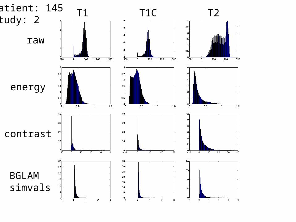
Patient: 145 Study: 2

T1 T1C T2

raw

energy

contrast

BGLAMsimvals

Patient: 145 Study: 2

Method

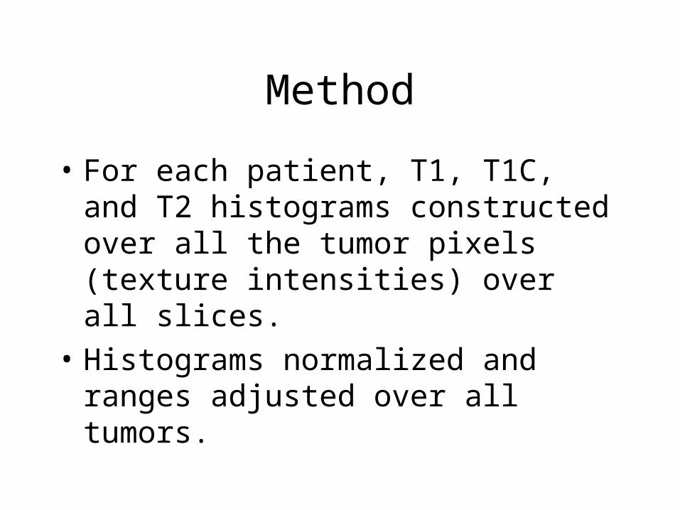
• For each patient, T1, T1C, and T2 histograms constructed over all the tumor pixels (texture intensities) over all slices.

• Histograms normalized and ranges adjusted over all tumors.

T1 T1C T2

raw

3rd MR8

6th MR8

7th MR8

Patient: 145 Study: 2

T1 T1C T2

raw

energy

contrast

BGLAMsimvals

Patient: 145 Study: 2

Method

• Each patient’s tumor is represented by a histogram for each modality and texture feature.

• The histograms are used as vector inputs to kmeans (k = 2) clustering.

Test Resultslowgrade/highgrade: mismatch rates

T1 T1C T2Raw 0.3600 0.3600 0.10001st MR8 0.2800 0.3800 0.40002nd MR8 0.2600 0.3800 0.42003rd MR8 0.4000 0.3800 0.28004th MR8 0.3000 0.3800 0.40005th MR8 0.2400 0.3600 0.40006th MR8 0.2800 0.3800 0.36007th MR8 0.3400 0.4000 0.12008th MR8 0.4000 0.4200 0.1400Energy 0.4400 0.3200 0.4600Contrast 0.3800 0.2800 0.4200BGLAM 0.3200 0.2000 0.4200

Test Resultsgbm/rest: mismatch rates

T1 T1C T20.3200 0.3200 0.14000.3600 0.4600 0.44000.3400 0.4600 0.42000.4800 0.4600 0.24000.3800 0.4600 0.48000.3200 0.4400 0.44000.3600 0.4600 0.36000.4200 0.4800 0.20000.4800 0.5000 0.22000.4400 0.3200 0.46000.3800 0.3600 0.38000.3200 0.2000 0.4200

Raw1st MR82nd MR83rd MR84th MR85th MR86th MR87th MR88th MR8EnergyContrastBGLAM

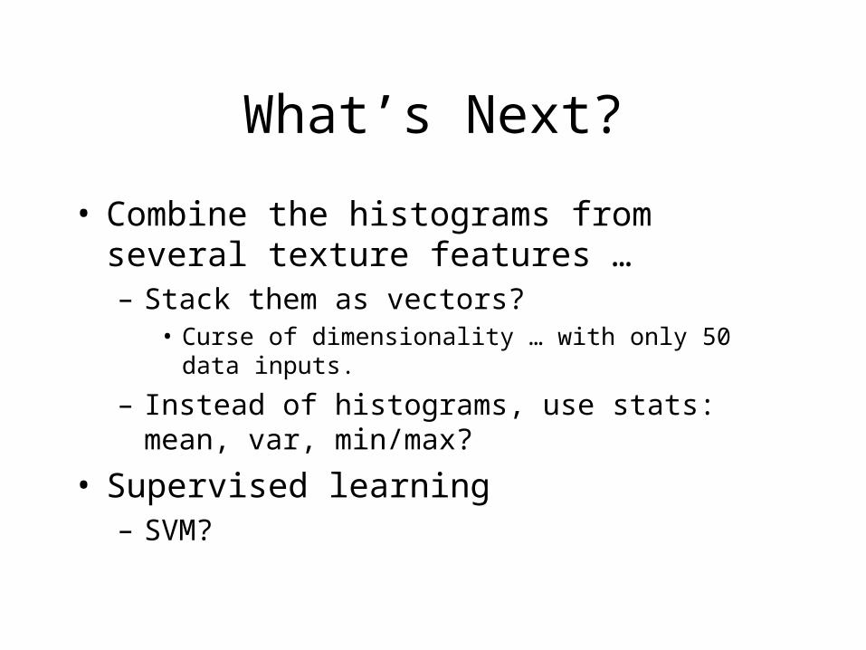
What’s Next?

• Combine the histograms from several texture features …– Stack them as vectors?

• Curse of dimensionality … with only 50 data inputs.

– Instead of histograms, use stats: mean, var, min/max?

• Supervised learning– SVM?