Embed Size (px)
Citation preview

Ivana Lucic Abstract
I
TRUCK MODELING ALONG GRADE SECTIONS
Ivana Lucic
Thesis submitted to the Faculty of the Virginia Polytechnic Institute and State University
in partial fulfillment of the requirements for the degree of
MASTER OF SCIENCE
IN
CIVIL AND ENVIRONMENTAL ENGINEERING
Dr. Hesham A. Rakha, Chairman
Dr. Antonio A. Trani
Dr. Imad L. Al-Qadi
May, 2001
Blacksburg, Virginia
Key words: Vehicle dynamics, traffic modeling, truck modeling, traffic flow theory.
Copyright 2001, Ivana Lucic

Lucic Abstract
I
TRUCK MODELING ALONG GRADE SECTIONS
Ivana Lucic
Abstract
This research effort first characterizes the trucks traveling along US highways by
analyzing data from Interstate 81. It is hypothesized that I-81 is typical of US highways
and thus can provide some insight into typical truck characteristics. These truck
characteristics are important for the development of an exhaustive vehicle performance
procedure. Analysis was done based on data collected at the Troutville weigh station. The
characterization involves an analysis of vehicle class distribution, GVW (Gross Vehicle
Weight) distribution, vehicle volume distribution, Average Weight on Tractive Axle
(AWTA), and typical weight-to-power ratios.
The thesis then assembles a database of systematic field data that can be utilized for the
validation of vehicle performance models. This database is unique because it was
conducted in a controlled field environment where the vehicle is only constrained by its
dynamics.
Using the assembled field database, a simple constant power vehicle dynamics model for
estimating maximum vehicle acceleration levels based on a vehicle’s tractive effort and
aerodynamic, rolling, and grade resistance forces was tested and validated. In addition,
typical model input parameters for different vehicle, pavement, and tire characteristics
are included in the thesis. The model was found to predict vehicle speeds at the
conclusion of the travel along the section to within 5 km/h (3.1 mi/h) of field
measurements, thus demonstrating the validity and applicability of the model.
Finally, the research effort introduces the concept of variable power in order to enhance
current state-of-the-art vehicle dynamics models and capture the build-up of power as a

Lucic Abstract
II
vehicle engages in gearshifts at low travel speeds. The proposed enhancement to the
current state-of-practice vehicle dynamics model allows the model to reflect typical
vehicle acceleration behavior more accurately. Subsequently, the model parameters are
calibrated using field measurements along a test roadway facility.

Lucic Acknowledgements
III
Acknowledgements
I would like to express my sincerest to Dr. Hesham A. Rakha, who serves as the
chairman of my thesis committee, for his guidance and financial support during my
graduate study and also for unselfish help to finish my thesis. I have learned a lot from
him during our together collaboration and this research would have not been finished
without him.
I gratefully would like to acknowledge Dr. Antonio A. Trani for helpful suggestions and
valuable knowledge given to me during my graduate education. I highly appreciate for
that and I admire his academic achievements. My thanks go to Dr. Imad L. Al-Qadi for
serving as my thesis committee member. Additionally, I would like to acknowledge him
for moral support through my work at the VTTI.
I would like to acknowledge the support of Virginia Department of Transportation
(VDOT) in supplying drivers for the validation data collection effort, especially the effort
of Kenneth Taylor and Kevin Light provided in driving the VDOT truck. Furthermore, I
would like to acknowledge Dr. Amara Loulizi for his technical support during data
collection on Smart Road, Mondher Chargui's efforts in collecting the GPS data, and also
Brent Crowther, Yihua Zhang, and Kyoungho Ahn for their help to conduct survey. In
addition, acknowledgements are due to Alejandra Medina and Dr. Francois Dion for
providing valuable input throughout the entire research effort. Finally, my acknowledge
goes to the Dr. Slimane Adjerid of the Math Department at Virginia Tech for his advice
provided in solving the Ordinary Differential Equation (ODE).
Most importantly, I would like to acknowledge my husband Panta Lucic for his love and
patient. My thanks to him for generous support and help through my study at Virginia
Tech. Furthermore, I am deeply indebted to my parents Ruza and Sava Ljubinkovic for
their wholehearted and unconditioned devotion in helping me seek my education abroad
and to my sister Tijana Ljubinkovic for her moral support and love. Without the love and
spiritual support from my family, would my goal have not been fulfilled.

Lucic Dedication
IV
Dedication
I would like to dedicate this thesis to my grate immediate family for their continuous
support and generous encouragement through my graduate study. To my splendid and
beloved husband Panta, this thesis is acknowledgment to his beautiful love, patient,
support and understanding for all the time that we did not spend together through my
study and this research.

Lucic TABLE OF CONTENTS
V
TABLE OF CONTENTS
CHAPTER 1: INTRODUCTION 1 1.1 PROBLEM DEFINITION............................................................................. 1 1.2 THESIS OBJECTIVE..................................................................................... 1 1.3 THESIS CONTRIBUTION........................................................................... 2 1.4 THESIS LAYOUT ............................................................................................ 3
CHAPTER 2: LITERATURE REVIEW 4 2.1 TRUCK CHARACTERISTICS EVOLUTION AND IMPACTS ON TRAFFIC FLOW ............................................................................................ 4 2.2 TRUCK IMPACTS ON PAVEMENT STRUCTURE ........................ 9 2.3 TRUCK MODELING ................................................................................... 11 2.4 WEIGH-IN-MOTION TECHNOLOGIES ........................................... 14 2.5 CONCLUSION ................................................................................................ 19
CHAPTER 3: I-81 TRUCK CHARACTERIZATION 20 3.1 FHWA TRUCK CLASSIFICATIONS ................................................... 21 3.2 TRUCK WEIGHT CHARACTERIZATION ...................................... 22
3.2.1 Data Collection Description ....................................................................... 22 3.2.2 Vehicle Class Distribution .......................................................................... 23 3.2.3 Truck Volume Distribution ........................................................................ 26 3.2.4 Gross Vehicle Weight Distribution............................................................ 35 3.2.6 Analysis of Variance (ANOVA) ................................................................. 43
3.3 SURVEY DATA .............................................................................................. 46 3.3.1 Consistency Between Sample and Population Trucks ........................... 46 3.3.2 Sample Vehicle Characterization .............................................................. 48
3.4 CONCLUSION ................................................................................................ 50 CHAPTER 4: BASIC VEHICLE DYNAMICS MODEL 52
4.1 TRACTIVE EFFORT ................................................................................... 53 4.2 RESISTANCE FORCES .............................................................................. 56 4.3 MAXIMUM VEHICLE ACCELERATION......................................... 59 4.4 MODEL VALIDATION............................................................................... 60
4.4.1 Test Truck Characteristics.......................................................................... 60 4.4.2 Study Section Description ........................................................................... 61 4.4.3 Test Run Execution ..................................................................................... 62 4.4.4 Test Run Description ................................................................................... 64 4.4.5 Model Validation Procedures and Results............................................... 64
4.5 UPDATED SAMPLE PERFORMANCE CURVES FOR DESIGN TRUCK ...................................................................................................................... 70 4.6 CONCLUSION ................................................................................................ 72
CHAPTER 5: VARIABLE POWER VEHICLE DYNAMICS MODEL 74

Lucic TABLE OF CONTENTS
VI
5.1 PROPOSED MODEL ENHANCEMENT ............................................. 74 5.2 VARIABLE POWER ADJUSTMENT FACTOR .............................. 79 5.3 CHARACTERIZATION OF TRUCKS ON US INTERSTATE HIGHWAYS ............................................................................................................ 85 5.4 MODEL CALIBRATION............................................................................ 87 5.5 CONCLUSION .............................................................................................. 100
CHAPTER 6: CONCLUSIONS AND RECCOMENDATION 101 6.1 PROBLEM OVERVIEW........................................................................... 101 6.2 THESIS SUMMARY ................................................................................... 102 6.3 THESIS CONTRIBUTIONS .................................................................... 102 6.4 THESIS CONCLUSIONS.......................................................................... 103 6.5 FUTURE RESEARCH................................................................................ 104
REFERENCES 105 APPENDIX A 109 APPENDIX B 122 APPENDIX C 181 APPENDIX D 202 VITA 229

Lucic LIST OF FIGURES
VII
LIST OF FIGURES
FIGURE 3.1: TRUCK PERCENTAGES BY VEHICLE CLASS FOR THREE YEARS................................ 24 FIGURE 3.2: TRUCK PERCENTAGES PER VEHICLE CLASS FOR AUGUST AND SEPTEMBER 2000 .... 25 FIGURE 3.3: SAMPLE OF TRUCK VOLUME DISTRIBUTION FOR SOUTHBOUND DIRECTION ............ 26 FIGURE 3.4: SAMPLE TRUCK VOLUME DISTRIBUTIONS PER MONTHS FOR BOTH DIRECTIONS ...... 28 FIGURE 3.5: TRUCK VOLUME DISTRIBUTIONS BY DAY-OF THE-WEEK FOR SEPTEMBER 2000...... 29 FIGURE 3.6: TRUCK VOLUME DISTRIBUTIONS BY HOUR FOR ALL VEHICLE CLASSES FOR
SEPTEMBER 2000 ......................................................................................................... 31 FIGURE 3.7: TRUCK VOLUME DISTRIBUTIONS BY HOUR FOR VEHICLE CLASS 9 FOR SEPTEMBER
2000............................................................................................................................ 32 FIGURE 3.8: TRUCK VOLUME DISTRIBUTIONS BY HOUR FOR ALL VEHICLE CLASSES FOR
SEPTEMBER 2000 ......................................................................................................... 33 FIGURE 3.9: TRUCK VOLUME DISTRIBUTIONS BY HOUR FOR VEHICLE CLASS 9 FOR SEPTEMBER
2000............................................................................................................................ 34 FIGURE 3.10: TRUCK WEIGHT DISTRIBUTIONS OVER THREE-YEAR PERIOD................................ 36 FIGURE 3.11: TRUCK WEIGHT DISTRIBUTIONS BY MONTH IN 2000 YEAR FOR ALL VEHICLE
CLASSES ...................................................................................................................... 37 FIGURE 3.12: TRUCK WEIGHT DISTRIBUTIONS BY MONTH IN 2000 YEAR FOR VEHICLE CLASS 9 . 38 FIGURE 3.13: TRUCK WEIGHT DISTRIBUTIONS FOR ALL VEHICLE CLASSES FOR SEPTEMBER 2000
................................................................................................................................... 39 FIGURE 3.14: TRUCK WEIGHT DISTRIBUTIONS FOR VEHICLE CLASS 9 FOR SEPTEMBER 2000...... 40 FIGURE 3.15: AVERAGE WEIGHT ON TRACTIVE AXLE BY YEAR ................................................ 41 FIGURE 3.16: AVERAGE WEIGHT ON TRACTIVE AXLE BY MONTH ............................................. 42 FIGURE 3.17: AVERAGE WEIGHT ON TRACTIVE AXLE BY DAY-OF-THE-WEEK............................ 43 FIGURE 3.18: VEHICLE CLASS PERCENTAGE COMPARISON OF SAMPLE AND WIM DATA ............ 47 FIGURE 3.19: VEHICLE WEIGHT DISTRIBUTION COMPARISON OF SAMPLE AND WIM DATA ........ 48 FIGURE 3.20: POWER DISTRIBUTION FOR ALL VEHICLE CLASSES AND CLASS 9.......................... 49 FIGURE 3.21: MASS DISTRIBUTION (VEHICLE CLASS NINE) ...................................................... 50 FIGURE 4.1: TRUCK PERFORMANCE CURVES FOR AN AVERAGE TRUCK (200 LB/HP) (HCM, 1997)
................................................................................................................................... 53 FIGURE 4.2: SMART ROAD TEST SECTION LAYOUT .................................................................. 63 FIGURE 4.3: PREDICTED AND OBSERVED SPEED PROFILE (9-LOAD CONFIGURATION) ................ 68 FIGURE 4.4: PREDICTED AND OBSERVED SPEED PROFILE (5-LOAD CONFIGURATION) ................ 69 FIGURE 4.5: PREDICTED AND OBSERVED SPEED PROFILE (1-LOAD CONFIGURATION) ................ 69 FIGURE 4.6: TRUCK PERFORMANCE CURVES FOR NTC-350 ENGINE (200 LB/HP)....................... 71 FIGURE 4.7: VARIATION IN CRAWL SPEED AS A FUNCTION OF ROADWAY GRADE FOR NTC-350
ENGINE........................................................................................................................ 72 FIGURE 5.1: SAMPLE TORQUE-POWER CURVES FOR A GASOLINE POWERED VEHICLE AND A TRUCK
................................................................................................................................... 77 FIGURE 5.2: SAMPLE TORQUE AND POWER CURVES FOR DIFFERENT GEARS (OLDSMOBILE
AURORA) .................................................................................................................... 78 FIGURE 5.3: VARIATION IN VEHICLE POWER AND ACCELERATION AS A FUNCTION OF SPEED...... 81 FIGURE 5.4: RELATIONSHIPS BETWEEN SPEED AT OPTIMUM POWER AND WEIGHT-TO-POWER
RATIOS ........................................................................................................................ 82

Lucic LIST OF FIGURES
VIII
FIGURE 5.5: SAMPLE ACCELERATION VERSUS SPEED PROFILE FOR 260 KW (350 HP) TRUCK ..... 83 FIGURE 5.6: SAMPLE ACCELERATION VERSUS DISTANCE PROFILE FOR 260 KW (350 HP) TRUCK 84 FIGURE 5:7: TRUCK CHARACTERIZATION AT I-81 TROUTVILLE WEIGH STATION....................... 86 FIGURE 5.8: SAMPLE SPEED PROFILE VALIDATION USING THE CONSTANT POWER MODEL (NTC-
350 ENGINE) ................................................................................................................ 91 FIGURE 5.9: SAMPLE SPEED PROFILE VALIDATION USING THE VARIABLE POWER MODEL........... 92 (NTC-350 ENGINE) .............................................................................................................. 92 FIGURE 5.10: SAMPLE SPEED PROFILE WITH THE BEST FIT USED FOR ERROR COMPUTING (NTC-
350 ENGINE) ................................................................................................................ 93 FIGURE 5.11: SAMPLE SPEED PROFILE COMPARING OBSERVED DATA WITH BOTH MODELS (NTC-
350 ENGINE) ................................................................................................................ 94 FIGURE 5.12: COMPARISON OF ERROR VERSUS DISTANCE TRAVELED FOR CONSTANT AND
VARIABLE POWER VEHICLE DYNAMIC MODELS............................................................... 95 FIGURE 5.13: SAMPLE SPEED PROFILE VALIDATION USING THE CONSTANT POWER MODEL (470 HP
ENGINE) ...................................................................................................................... 97 FIGURE 5.14: SAMPLE SPEED PROFILE VALIDATION USING THE VARIABLE POWER MODEL (470 HP
ENGINE) ...................................................................................................................... 98 FIGURE 5.15: TRUCK PERFORMANCE CURVES FOR NTC-350 ENGINE (200 LB/HP)..................... 99 FIGURE A.1: SURVEY QUESTIONER...................................................................................... 110 FIGURE B.1: PREDICTED AND OBSERVED SPEED PROFILE (9-LOAD CONFIGURATION) ............ 126 FIGURE B.2: PREDICTED AND OBSERVED SPEED PROFILE (8-LOAD CONFIGURATION) ............ 126 FIGURE B.3: PREDICTED AND OBSERVED SPEED PROFILE (7-LOAD CONFIGURATION) ............ 127 FIGURE B.4: PREDICTED AND OBSERVED SPEED PROFILE (6-LOAD CONFIGURATION) ............ 127 FIGURE B.5: PREDICTED AND OBSERVED SPEED PROFILE (5-LOAD CONFIGURATION) ............ 127 FIGURE B.6: PREDICTED AND OBSERVED SPEED PROFILE (4-LOAD CONFIGURATION) ............ 128 FIGURE B.7: PREDICTED AND OBSERVED SPEED PROFILE (3-LOAD CONFIGURATION) ............ 128 FIGURE B.8: PREDICTED AND OBSERVED SPEED PROFILE (2-LOAD CONFIGURATION) ............ 128 FIGURE B.9: PREDICTED AND OBSERVED SPEED PROFILE (1-LOAD CONFIGURATION) ............ 129 FIGURE B.10: PREDICTED AND OBSERVED SPEED PROFILE (0-LOAD CONFIGURATION) .......... 129 FIGURE B.11: PREDICTED AND OBSERVED SPEED PROFILE (9-LOAD CONFIGURATION) .......... 133 FIGURE B.12: PREDICTED AND OBSERVED SPEED PROFILE (8-LOAD CONFIGURATION) .......... 134 FIGURE B.13: PREDICTED AND OBSERVED SPEED PROFILE (7-LOAD CONFIGURATION) .......... 134 FIGURE B.14: PREDICTED AND OBSERVED SPEED PROFILE (6-LOAD CONFIGURATION) .......... 134 FIGURE B.15: PREDICTED AND OBSERVED SPEED PROFILE (5-LOAD CONFIGURATION) .......... 135 FIGURE B.16: PREDICTED AND OBSERVED SPEED PROFILE (4-LOAD CONFIGURATION) .......... 135 FIGURE B.17: PREDICTED AND OBSERVED SPEED PROFILE (3-LOAD CONFIGURATION) .......... 135 FIGURE B.18: PREDICTED AND OBSERVED SPEED PROFILE (2-LOAD CONFIGURATION) .......... 136 FIGURE B.19: PREDICTED AND OBSERVED SPEED PROFILE (1-LOAD CONFIGURATION) .......... 136 FIGURE B.20: PREDICTED AND OBSERVED SPEED PROFILE (0-LOAD CONFIGURATION) .......... 136 FIGURE B.21: PREDICTED AND OBSERVED SPEED PROFILE (TRUCK CONFIGURATION) ........... 137 FIGURE B.22: PREDICTED AND OBSERVED SPEED PROFILE (9-LOAD CONFIGURATION) .......... 141 FIGURE B.23: PREDICTED AND OBSERVED SPEED PROFILE (8-LOAD CONFIGURATION) .......... 141 FIGURE B.24: PREDICTED AND OBSERVED SPEED PROFILE (7-LOAD CONFIGURATION) .......... 141 FIGURE B.25: PREDICTED AND OBSERVED SPEED PROFILE (6-LOAD CONFIGURATION) .......... 142 FIGURE B.26: PREDICTED AND OBSERVED SPEED PROFILE (5-LOAD CONFIGURATION) .......... 142 FIGURE B.27: PREDICTED AND OBSERVED SPEED PROFILE (4-LOAD CONFIGURATION) .......... 142 FIGURE B.28: PREDICTED AND OBSERVED SPEED PROFILE (3-LOAD CONFIGURATION) .......... 143

Lucic LIST OF FIGURES
IX
FIGURE B.29: PREDICTED AND OBSERVED SPEED PROFILE (2-LOAD CONFIGURATION) .......... 143 FIGURE B.30: PREDICTED AND OBSERVED SPEED PROFILE (1-LOAD CONFIGURATION) .......... 143 FIGURE B.31: PREDICTED AND OBSERVED SPEED PROFILE (0-LOAD CONFIGURATION) .......... 144 FIGURE B.32: PREDICTED AND OBSERVED SPEED PROFILE (TRUCK CONFIGURATION) ........... 144 FIGURE B.33: PREDICTED AND OBSERVED SPEED PROFILE (9-LOAD CONFIGURATION) .......... 148 FIGURE B.34: PREDICTED AND OBSERVED SPEED PROFILE (8-LOAD CONFIGURATION) .......... 148 FIGURE B.35: PREDICTED AND OBSERVED SPEED PROFILE (7-LOAD CONFIGURATION) .......... 149 FIGURE B.36: PREDICTED AND OBSERVED SPEED PROFILE (6-LOAD CONFIGURATION) .......... 149 FIGURE B.37: PREDICTED AND OBSERVED SPEED PROFILE (5-LOAD CONFIGURATION) .......... 149 FIGURE B.38: PREDICTED AND OBSERVED SPEED PROFILE (4-LOAD CONFIGURATION) .......... 150 FIGURE B.39: PREDICTED AND OBSERVED SPEED PROFILE (3-LOAD CONFIGURATION) .......... 150 FIGURE B.40: PREDICTED AND OBSERVED SPEED PROFILE (2-LOAD CONFIGURATION) .......... 150 FIGURE B.41: PREDICTED AND OBSERVED SPEED PROFILE (1-LOAD CONFIGURATION) .......... 151 FIGURE B.42: PREDICTED AND OBSERVED SPEED PROFILE (0-LOAD CONFIGURATION) .......... 151 FIGURE B.43: PREDICTED AND OBSERVED SPEED PROFILE (9-LOAD CONFIGURATION) .......... 155 FIGURE B.44: PREDICTED AND OBSERVED SPEED PROFILE (8-LOAD CONFIGURATION) .......... 155 FIGURE B.45: PREDICTED AND OBSERVED SPEED PROFILE (7-LOAD CONFIGURATION) .......... 156 FIGURE B.46: PREDICTED AND OBSERVED SPEED PROFILE (6-LOAD CONFIGURATION) .......... 156 FIGURE B.47: PREDICTED AND OBSERVED SPEED PROFILE (5-LOAD CONFIGURATION) .......... 156 FIGURE B.48: PREDICTED AND OBSERVED SPEED PROFILE (4-LOAD CONFIGURATION) .......... 157 FIGURE B.49: PREDICTED AND OBSERVED SPEED PROFILE (3-LOAD CONFIGURATION) .......... 157 FIGURE B.50: PREDICTED AND OBSERVED SPEED PROFILE (2-LOAD CONFIGURATION) .......... 157 FIGURE B.51: PREDICTED AND OBSERVED SPEED PROFILE (1-LOAD CONFIGURATION) .......... 158 FIGURE B.52: PREDICTED AND OBSERVED SPEED PROFILE (0-LOAD CONFIGURATION) .......... 158 FIGURE B.53: PREDICTED AND OBSERVED SPEED PROFILE (9-LOAD CONFIGURATION) .......... 162 FIGURE B.54: PREDICTED AND OBSERVED SPEED PROFILE (8-LOAD CONFIGURATION) .......... 163 FIGURE B.55: PREDICTED AND OBSERVED SPEED PROFILE (7-LOAD CONFIGURATION) .......... 163 FIGURE B.56: PREDICTED AND OBSERVED SPEED PROFILE (6-LOAD CONFIGURATION) .......... 163 FIGURE B.57: PREDICTED AND OBSERVED SPEED PROFILE (5-LOAD CONFIGURATION) .......... 164 FIGURE B.58: PREDICTED AND OBSERVED SPEED PROFILE (4-LOAD CONFIGURATION) .......... 164 FIGURE B.59: PREDICTED AND OBSERVED SPEED PROFILE (3-LOAD CONFIGURATION) .......... 164 FIGURE B.60: PREDICTED AND OBSERVED SPEED PROFILE (2-LOAD CONFIGURATION) .......... 165 FIGURE B.61: PREDICTED AND OBSERVED SPEED PROFILE (1-LOAD CONFIGURATION) .......... 165 FIGURE B.62: PREDICTED AND OBSERVED SPEED PROFILE (0-LOAD CONFIGURATION) .......... 165 FIGURE B.63: PREDICTED AND OBSERVED SPEED PROFILE (TRUCK CONFIGURATION) ........... 166 FIGURE B.64: PREDICTED AND OBSERVED SPEED PROFILE (9-LOAD CONFIGURATION) .......... 170 FIGURE B.65: PREDICTED AND OBSERVED SPEED PROFILE (8-LOAD CONFIGURATION) .......... 170 FIGURE B.66: PREDICTED AND OBSERVED SPEED PROFILE (7-LOAD CONFIGURATION) .......... 170 FIGURE B.67: PREDICTED AND OBSERVED SPEED PROFILE (6-LOAD CONFIGURATION) .......... 171 FIGURE B.68: PREDICTED AND OBSERVED SPEED PROFILE (5-LOAD CONFIGURATION) .......... 171 FIGURE B.69: PREDICTED AND OBSERVED SPEED PROFILE (4-LOAD CONFIGURATION) .......... 171 FIGURE B.70: PREDICTED AND OBSERVED SPEED PROFILE (3-LOAD CONFIGURATION) .......... 172 FIGURE B.71: PREDICTED AND OBSERVED SPEED PROFILE (2-LOAD CONFIGURATION) .......... 172 FIGURE B.72: PREDICTED AND OBSERVED SPEED PROFILE (1-LOAD CONFIGURATION) .......... 172 FIGURE B.73: PREDICTED AND OBSERVED SPEED PROFILE (0-LOAD CONFIGURATION) .......... 173 FIGURE B.74: PREDICTED AND OBSERVED SPEED PROFILE (TRUCK CONFIGURATION) ........... 173

Lucic LIST OF FIGURES
X
FIGURE B.75: PREDICTED AND OBSERVED SPEED PROFILE (9-LOAD CONFIGURATION) .......... 177 FIGURE B.76: PREDICTED AND OBSERVED SPEED PROFILE (8-LOAD CONFIGURATION) .......... 177 FIGURE B.77: PREDICTED AND OBSERVED SPEED PROFILE (7-LOAD CONFIGURATION) .......... 178 FIGURE B.78: PREDICTED AND OBSERVED SPEED PROFILE (6-LOAD CONFIGURATION) .......... 178 FIGURE B.79: PREDICTED AND OBSERVED SPEED PROFILE (5-LOAD CONFIGURATION) .......... 178 FIGURE B.80: PREDICTED AND OBSERVED SPEED PROFILE (4-LOAD CONFIGURATION) .......... 179 FIGURE B.81: PREDICTED AND OBSERVED SPEED PROFILE (3-LOAD CONFIGURATION) .......... 179 FIGURE B.82: PREDICTED AND OBSERVED SPEED PROFILE (2-LOAD CONFIGURATION) .......... 179 FIGURE B.83: PREDICTED AND OBSERVED SPEED PROFILE (1-LOAD CONFIGURATION) .......... 180 FIGURE B.84: PREDICTED AND OBSERVED SPEED PROFILE (0-LOAD CONFIGURATION) .......... 180 FIGURE C.1: COMPARISON OF ERROR VERSUS DISTANCE TRAVELED (9-LOAD CONFIGURATION)
................................................................................................................................. 186 FIGURE C.2: COMPARISON OF ERROR VERSUS DISTANCE TRAVELED (8-LOAD CONFIGURATION)
................................................................................................................................. 186 FIGURE C.3: COMPARISON OF ERROR VERSUS DISTANCE TRAVELED (7-LOAD CONFIGURATION)
................................................................................................................................. 187 FIGURE C.4: COMPARISON OF ERROR VERSUS DISTANCE TRAVELED (6-LOAD CONFIGURATION)
................................................................................................................................. 187 FIGURE C.5: COMPARISON OF ERROR VERSUS DISTANCE TRAVELED (5-LOAD CONFIGURATION)
................................................................................................................................. 187 FIGURE C.6: COMPARISON OF ERROR VERSUS DISTANCE TRAVELED (4-LOAD CONFIGURATION)
................................................................................................................................. 188 FIGURE C.7: COMPARISON OF ERROR VERSUS DISTANCE TRAVELED (3-LOAD CONFIGURATION)
................................................................................................................................. 188 FIGURE C.8: COMPARISON OF ERROR VERSUS DISTANCE TRAVELED (2-LOAD CONFIGURATION)
................................................................................................................................. 188 FIGURE C.9: COMPARISON OF ERROR VERSUS DISTANCE TRAVELED (1-LOAD CONFIGURATION)
................................................................................................................................. 189 FIGURE C.10: COMPARISON OF ERROR VERSUS DISTANCE TRAVELED (0-LOAD CONFIGURATION)
................................................................................................................................. 189 FIGURE C.11: COMPARISON OF ERROR VERSUS DISTANCE TRAVELED (9-LOAD CONFIGURATION)
................................................................................................................................. 190 FIGURE C.12: COMPARISON OF ERROR VERSUS DISTANCE TRAVELED (8-LOAD CONFIGURATION)
................................................................................................................................. 190 FIGURE C.13: COMPARISON OF ERROR VERSUS DISTANCE TRAVELED (7-LOAD CONFIGURATION)
................................................................................................................................. 190 FIGURE C.14: COMPARISON OF ERROR VERSUS DISTANCE TRAVELED (6-LOAD CONFIGURATION)
................................................................................................................................. 191 FIGURE C.15: COMPARISON OF ERROR VERSUS DISTANCE TRAVELED (5-LOAD CONFIGURATION)
................................................................................................................................. 191 FIGURE C.16: COMPARISON OF ERROR VERSUS DISTANCE TRAVELED (4-LOAD CONFIGURATION)
................................................................................................................................. 191 FIGURE C.17: COMPARISON OF ERROR VERSUS DISTANCE TRAVELED (3-LOAD CONFIGURATION)
................................................................................................................................. 192 FIGURE C.18: COMPARISON OF ERROR VERSUS DISTANCE TRAVELED (2-LOAD CONFIGURATION)
................................................................................................................................. 192 FIGURE C.19: COMPARISON OF ERROR VERSUS DISTANCE TRAVELED (1-LOAD CONFIGURATION)
................................................................................................................................. 192

Lucic LIST OF FIGURES
XI
FIGURE C.20: COMPARISON OF ERROR VERSUS DISTANCE TRAVELED (0-LOAD CONFIGURATION)................................................................................................................................. 193
FIGURE C.21: COMPARISON OF ERROR VERSUS DISTANCE TRAVELED (TRUCK CONFIGURATION)................................................................................................................................. 193
FIGURE C.22: COMPARISON OF ERROR VERSUS DISTANCE TRAVELED (9–LOAD CONFIGURATION)................................................................................................................................. 194
FIGURE C.23: COMPARISON OF ERROR VERSUS DISTANCE TRAVELED (8–LOAD CONFIGURATION)................................................................................................................................. 194
FIGURE C.24: COMPARISON OF ERROR VERSUS DISTANCE TRAVELED (7–LOAD CONFIGURATION)................................................................................................................................. 194
FIGURE C.25: COMPARISON OF ERROR VERSUS DISTANCE TRAVELED (6–LOAD CONFIGURATION)................................................................................................................................. 195
FIGURE C.26: COMPARISON OF ERROR VERSUS DISTANCE TRAVELED (5–LOAD CONFIGURATION)................................................................................................................................. 195
FIGURE C.27: COMPARISON OF ERROR VERSUS DISTANCE TRAVELED (4–LOAD CONFIGURATION)................................................................................................................................. 195
FIGURE C.28: COMPARISON OF ERROR VERSUS DISTANCE TRAVELED (3–LOAD CONFIGURATION)................................................................................................................................. 196
FIGURE C.29: COMPARISON OF ERROR VERSUS DISTANCE TRAVELED (2–LOAD CONFIGURATION)................................................................................................................................. 196
FIGURE C.30: COMPARISON OF ERROR VERSUS DISTANCE TRAVELED (1–LOAD CONFIGURATION)................................................................................................................................. 196
FIGURE C.31: COMPARISON OF ERROR VERSUS DISTANCE TRAVELED (0–LOAD CONFIGURATION)................................................................................................................................. 197
FIGURE C.32: COMPARISON OF ERROR VERSUS DISTANCE TRAVELED (TRUCK CONFIGURATION)................................................................................................................................. 197
FIGURE C.33: COMPARISON OF ERROR VERSUS DISTANCE TRAVELED (9–LOAD CONFIGURATION)................................................................................................................................. 198
FIGURE C.34: COMPARISON OF ERROR VERSUS DISTANCE TRAVELED (8–LOAD CONFIGURATION)................................................................................................................................. 198
FIGURE C.35: COMPARISON OF ERROR VERSUS DISTANCE TRAVELED (7–LOAD CONFIGURATION)................................................................................................................................. 198
FIGURE C.36: COMPARISON OF ERROR VERSUS DISTANCE TRAVELED (6–LOAD CONFIGURATION)................................................................................................................................. 199
FIGURE C.37: COMPARISON OF ERROR VERSUS DISTANCE TRAVELED (5–LOAD CONFIGURATION)................................................................................................................................. 199
FIGURE C.38: COMPARISON OF ERROR VERSUS DISTANCE TRAVELED (4–LOAD CONFIGURATION)................................................................................................................................. 199
FIGURE C.39: COMPARISON OF ERROR VERSUS DISTANCE TRAVELED (3–LOAD CONFIGURATION)................................................................................................................................. 200
FIGURE C.40: COMPARISON OF ERROR VERSUS DISTANCE TRAVELED (2–LOAD CONFIGURATION)................................................................................................................................. 200
FIGURE C.41: COMPARISON OF ERROR VERSUS DISTANCE TRAVELED (1–LOAD CONFIGURATION)................................................................................................................................. 200
FIGURE C.42: COMPARISON OF ERROR VERSUS DISTANCE TRAVELED (0–LOAD CONFIGURATION)................................................................................................................................. 201

Lucic LIST OF TABLES
XII
LIST OF TABLES
TABLE 3.1: DAYS WHICH DATA WERE ANALYZED .............................................................. 22 TABLE 3.2: TRUCK VOLUMES BY DAY-OF-THE-WEEK FOR ALL VEHICLE CLASSES OVER THE
THREE-YEAR PERIOD .................................................................................................. 27 TABLE 3.3: TRUCK VOLUMES BY DAY-OF-THE-WEEK FOR VEHICLE CLASS 9 OVER THE
THREE-YEAR PERIOD .................................................................................................. 27 TABLE 3.4: PERCENT OF VEHICLE FREQUENCY FOR AUGUST 2000..................................... 29 TABLE 3.5: PERCENT OF VEHICLE FREQUENCY FOR SEPTEMBER 2000 ............................... 30 TABLE 3.6: SUMMARIZED DATA FOR ANOVA TEST.......................................................... 44 TABLE 3.7: MEAN MASS VARIATIONS BY DAY-OF-THE-WEEK FOR GVW ........................... 45 TABLE 3.8: MEAN MASS VARIATIONS BY MONTH OF THE YEAR FOR GVW......................... 45 TABLE 3.9: MEAN MASS VARIATIONS BY DAY-OF-THE-WEEK FOR AWTA......................... 45 TABLE 3.10: MEAN MASS VARIATIONS BY MONTH OF THE YEAR FOR AWTA .................... 46 TABLE 3.11: SUMMARIZED DATA FOR VEHICLE CLASSIFICATION FROM SAMPLE AND WIM
STATION ..................................................................................................................... 47 TABLE 4.1: MODEL VARIABLES AND COEFFICIENTS ........................................................... 54 TABLE 4.2: TRANSMISSION EFFICIENCY (SAE J2188, 1996).............................................. 55 TABLE 4.3: LENGTH AND MASS DISTRIBUTION FOR TYPICAL TRUCKS (FITCH, 1994).......... 56 TABLE 4.4: TYPICAL VEHICLE FRONTAL AREAS (SAE J2188, 1996).................................. 57 TABLE 4.5: TYPICAL VEHICLE DRAG COEFFICIENTS ........................................................... 57 TABLE 4.6: HIGHWAY SURFACE COEFFICIENTS (DERIVED FROM FITCH, 1994)................... 58 TABLE 4.7: ROLLING RESISTANCE CONSTANTS .................................................................. 58 TABLE 4.8: TRUCK AND TRAILER AXLE’S MASS ANALYZED ............................................... 64 TABLE 4.9: MODEL PARAMETERS UTILIZED IN ANALYSIS................................................... 65 TABLE 4.10: EXAMPLE SOLUTION TO ODE (9-LOAD CONFIGURATION) ............................ 67 TABLE 5.1: TEST TRUCK CHARACTERISTICS ....................................................................... 87 TABLE 5.2: TRUCK WEIGHT-TO-POWER EXPERIMENTAL DESIGN (KG/KW) ......................... 88 TABLE 5.3: EXAMPLE SOLUTION TO ODE (9-LOAD CONFIGURATION) .............................. 89 TABLE 5.4: EXAMPLE SOLUTION TO ODE (1-LOAD CONFIGURATION) .............................. 90 TABLE 5.5: COMPUTED OPTIMUM SPEEDS FOR DIFFERENT TRUCKS AND LOAD
CONFIGURATIONS ....................................................................................................... 96 TABLE 5.6: MEAN SQUARE ERRORS FOR CONSTANT VEHICLE DYNAMIC MODEL................. 96 TABLE 5.7: MEAN SQUARE ERRORS FOR VARIABLE VEHICLE DYNAMIC MODEL.................. 96 TABLE 5.8: DIFFERENCE IN ERROR COMPUTED FOR BOTH MODELS................................... 100 31. ROESS, R.P.; MESSER, C.J. (1984) ‘PASSENGER CAR EQUIVALENTS FOR
UNINTERRUPTED FLOW: REVISION OF CIRCULAR 212 VALUES’. TRANSPORTATION RESEARCH RECORD 971, P. 7-13.............................................................................. 107
TABLE A.1: SURVEY DATA............................................................................................... 111 TABLE A.1: SURVEY DATA (CONTINUED) ........................................................................ 112 TABLE A.1: SURVEY DATA (CONTINUED) ........................................................................ 113 TABLE A.1: SURVEY DATA (CONTINUED) ........................................................................ 114 TABLE A.1: SURVEY DATA (CONTINUED) ........................................................................ 115 TABLE A.1: SURVEY DATA (CONTINUED) ........................................................................ 116

Lucic LIST OF TABLES
XIII
TABLE A.2: DATA LEGEND .............................................................................................. 117 TABLE A.3: SUMMARIZED DATA FROM SURVEY FOR VEHICLE CLASS NINE ...................... 118 TABLE A.3: SUMMARIZED DATA FROM SURVEY FOR VEHICLE CLASS NINE (CONTINUED) 119 TABLE A.3: SUMMARIZED DATA FROM SURVEY FOR VEHICLE CLASS NINE (CONTINUED) 120 TABLE A.3: SUMMARIZED DATA FROM SURVEY FOR VEHICLE CLASS NINE (CONTINUED) 121 TABLE B.1: EXAMPLE SOLUTION TO ODE (9-LOAD CONFIGURATION) ........................... 123 TABLE B.2: EXAMPLE SOLUTION TO ODE (8-LOAD CONFIGURATION) ........................... 123 TABLE B.3: EXAMPLE SOLUTION TO ODE (7-LOAD CONFIGURATION)............................ 123 TABLE B.4: EXAMPLE SOLUTION TO ODE (6-LOAD CONFIGURATION) ........................... 124 TABLE B.5: EXAMPLE SOLUTION TO ODE (5-LOAD CONFIGURATION) ........................... 124 TABLE B.6: EXAMPLE SOLUTION TO ODE (4-LOAD CONFIGURATION) ........................... 124 TABLE B.7: EXAMPLE SOLUTION TO ODE (3-LOAD CONFIGURATION) ........................... 125 TABLE B.8: EXAMPLE SOLUTION TO ODE (2-LOAD CONFIGURATION) ........................... 125 TABLE B.9: EXAMPLE SOLUTION TO ODE (1-LOAD CONFIGURATION) ........................... 125 TABLE B.10: EXAMPLE SOLUTION TO ODE (0-LOAD CONFIGURATION) ......................... 126 TABLE B.11: EXAMPLE SOLUTION TO ODE (9-LOAD CONFIGURATION) ......................... 130 TABLE B.12: EXAMPLE SOLUTION TO ODE (8-LOAD CONFIGURATION) ......................... 130 TABLE B.13: EXAMPLE SOLUTION TO ODE (7-LOAD CONFIGURATION) ......................... 130 TABLE B.14: EXAMPLE SOLUTION TO ODE (6-LOAD CONFIGURATION) ......................... 131 TABLE B.15: EXAMPLE SOLUTION TO ODE (5-LOAD CONFIGURATION) ......................... 131 TABLE B.16: EXAMPLE SOLUTION TO ODE (4-LOAD CONFIGURATION) ......................... 131 TABLE B.17: EXAMPLE SOLUTION TO ODE (3-LOAD CONFIGURATION) ......................... 132 TABLE B.18: EXAMPLE SOLUTION TO ODE (2-LOAD CONFIGURATION) ......................... 132 TABLE B.19: EXAMPLE SOLUTION TO ODE (1-LOAD CONFIGURATION) ......................... 132 TABLE B.20: EXAMPLE SOLUTION TO ODE (0-LOAD CONFIGURATION) ......................... 133 TABLE B.21: EXAMPLE SOLUTION TO ODE (TRUCK CONFIGURATION)........................... 133 TABLE B.22: EXAMPLE SOLUTION TO ODE (9-LOAD CONFIGURATION) ......................... 137 TABLE B.23: EXAMPLE SOLUTION TO ODE (8-LOAD CONFIGURATION) ......................... 137 TABLE B.24: EXAMPLE SOLUTION TO ODE (7-LOAD CONFIGURATION) ......................... 138 TABLE B.25: EXAMPLE SOLUTION TO ODE (6-LOAD CONFIGURATION) ......................... 138 TABLE B.26: EXAMPLE SOLUTION TO ODE (5-LOAD CONFIGURATION) ......................... 138 TABLE B.27: EXAMPLE SOLUTION TO ODE (4-LOAD CONFIGURATION) ......................... 139 TABLE B.28: EXAMPLE SOLUTION TO ODE (3-LOAD CONFIGURATION) ......................... 139 TABLE B.29: EXAMPLE SOLUTION TO ODE (2-LOAD CONFIGURATION) ......................... 139 TABLE B.30: EXAMPLE SOLUTION TO ODE (1-LOAD CONFIGURATION) ......................... 140 TABLE B.31: EXAMPLE SOLUTION TO ODE (0-LOAD CONFIGURATION) ......................... 140 TABLE B.32: EXAMPLE SOLUTION TO ODE (TRUCK CONFIGURATION)........................... 140 TABLE B.33: EXAMPLE SOLUTION TO ODE (9-LOAD CONFIGURATION) ......................... 145 TABLE B.34: EXAMPLE SOLUTION TO ODE (8-LOAD CONFIGURATION) ......................... 145 TABLE B.35: EXAMPLE SOLUTION TO ODE (7-LOAD CONFIGURATION) ......................... 145 TABLE B.36: EXAMPLE SOLUTION TO ODE (6-LOAD CONFIGURATION) ......................... 146 TABLE B.37: EXAMPLE SOLUTION TO ODE (5-LOAD CONFIGURATION) ......................... 146 TABLE B.38: EXAMPLE SOLUTION TO ODE (4-LOAD CONFIGURATION) ......................... 146 TABLE B.39: EXAMPLE SOLUTION TO ODE (3-LOAD CONFIGURATION) ......................... 147 TABLE B.40: EXAMPLE SOLUTION TO ODE (2-LOAD CONFIGURATION) ......................... 147 TABLE B.41: EXAMPLE SOLUTION TO ODE (1-LOAD CONFIGURATION) ......................... 147

Lucic LIST OF TABLES
XIV
TABLE B.42: EXAMPLE SOLUTION TO ODE (0-LOAD CONFIGURATION) ......................... 148 TABLE B.43: EXAMPLE SOLUTION TO ODE (9-LOAD CONFIGURATION) ......................... 152 TABLE B.44: EXAMPLE SOLUTION TO ODE (8-LOAD CONFIGURATION) ......................... 152 TABLE B.45: EXAMPLE SOLUTION TO ODE (7-LOAD CONFIGURATION) ......................... 152 TABLE B.46: EXAMPLE SOLUTION TO ODE (6-LOAD CONFIGURATION) ......................... 153 TABLE B.47: EXAMPLE SOLUTION TO ODE (5-LOAD CONFIGURATION) ......................... 153 TABLE B.48: EXAMPLE SOLUTION TO ODE (4-LOAD CONFIGURATION) ......................... 153 TABLE B.49: EXAMPLE SOLUTION TO ODE (3-LOAD CONFIGURATION) ......................... 154 TABLE B.50: EXAMPLE SOLUTION TO ODE (2-LOAD CONFIGURATION) ......................... 154 TABLE B.51: EXAMPLE SOLUTION TO ODE (1-LOAD CONFIGURATION) ......................... 154 TABLE B.52: EXAMPLE SOLUTION TO ODE (0-LOAD CONFIGURATION) ......................... 155 TABLE B.53: EXAMPLE SOLUTION TO ODE (9-LOAD CONFIGURATION) ......................... 159 TABLE B.54: EXAMPLE SOLUTION TO ODE (8-LOAD CONFIGURATION) ......................... 159 TABLE B.55: EXAMPLE SOLUTION TO ODE (7-LOAD CONFIGURATION) ......................... 159 TABLE B.56: EXAMPLE SOLUTION TO ODE (6-LOAD CONFIGURATION) ......................... 160 TABLE B.57: EXAMPLE SOLUTION TO ODE (5-LOAD CONFIGURATION) ......................... 160 TABLE B.58: EXAMPLE SOLUTION TO ODE (4-LOAD CONFIGURATION) ......................... 160 TABLE B.59: EXAMPLE SOLUTION TO ODE (3-LOAD CONFIGURATION) ......................... 161 TABLE B.60: EXAMPLE SOLUTION TO ODE (2-LOAD CONFIGURATION) ......................... 161 TABLE B.61: EXAMPLE SOLUTION TO ODE (1-LOAD CONFIGURATION) ......................... 161 TABLE B.62: EXAMPLE SOLUTION TO ODE (0-LOAD CONFIGURATION) ......................... 162 TABLE B.63: EXAMPLE SOLUTION TO ODE (TRUCK CONFIGURATION)........................... 162 TABLE B.64: EXAMPLE SOLUTION TO ODE (9-LOAD CONFIGURATION) ......................... 166 TABLE B.65: EXAMPLE SOLUTION TO ODE (8-LOAD CONFIGURATION) ......................... 166 TABLE B.66: EXAMPLE SOLUTION TO ODE (7-LOAD CONFIGURATION) ......................... 167 TABLE B.67: EXAMPLE SOLUTION TO ODE (6-LOAD CONFIGURATION) ......................... 167 TABLE B.68: EXAMPLE SOLUTION TO ODE (5-LOAD CONFIGURATION) ......................... 167 TABLE B.69: EXAMPLE SOLUTION TO ODE (4-LOAD CONFIGURATION) ......................... 168 TABLE B.70: EXAMPLE SOLUTION TO ODE (3-LOAD CONFIGURATION) ......................... 168 TABLE B.71: EXAMPLE SOLUTION TO ODE (2-LOAD CONFIGURATION) ......................... 168 TABLE B.72: EXAMPLE SOLUTION TO ODE (1-LOAD CONFIGURATION) ......................... 169 TABLE B.73: EXAMPLE SOLUTION TO ODE (0-LOAD CONFIGURATION) ......................... 169 TABLE B.74: EXAMPLE SOLUTION TO ODE (TRUCK CONFIGURATION)........................... 169 TABLE B.75: EXAMPLE SOLUTION TO ODE (9-LOAD CONFIGURATION) ......................... 174 TABLE B.76: EXAMPLE SOLUTION TO ODE (8-LOAD CONFIGURATION) ......................... 174 TABLE B.77: EXAMPLE SOLUTION TO ODE (7-LOAD CONFIGURATION) ......................... 174 TABLE B.78: EXAMPLE SOLUTION TO ODE (6-LOAD CONFIGURATION) ......................... 175 TABLE B.79: EXAMPLE SOLUTION TO ODE (5-LOAD CONFIGURATION) ......................... 175 TABLE B.80: EXAMPLE SOLUTION TO ODE (4-LOAD CONFIGURATION) ......................... 175 TABLE B.81: EXAMPLE SOLUTION TO ODE (3-LOAD CONFIGURATION) ......................... 176 TABLE B.82: EXAMPLE SOLUTION TO ODE (2-LOAD CONFIGURATION) ......................... 176 TABLE B.83: EXAMPLE SOLUTION TO ODE (1-LOAD CONFIGURATION) ......................... 176 TABLE B.84: EXAMPLE SOLUTION TO ODE (0-LOAD CONFIGURATION) ......................... 177 TABLE D.1: MEAN MASS (KG) VARIATIONS BY DOW, DIRECTION, SEASON, AND MONTH
FOR 1998 YEAR ........................................................................................................ 203

Lucic LIST OF TABLES
XV
TABLE D.1: MEAN MASS (KG) VARIATIONS BY DOW, DIRECTION, SEASON, AND MONTH FOR 1998 YEAR (CONTINUED).................................................................................. 204
TABLE D.2: MEAN MASS (KG) VARIATIONS BY DOW, DIRECTION, SEASON, AND MONTH FOR 1999 YEAR ........................................................................................................ 205
TABLE D.2: MEAN MASS (KG) VARIATIONS BY DOW, DIRECTION, SEASON, AND MONTH FOR 1999 YEAR (CONTINUED).................................................................................. 206
TABLE D.3: MEAN MASS (KG) VARIATIONS BY DOW, DIRECTION, SEASON, AND MONTH FOR 2000 YEAR ........................................................................................................ 207
TABLE D.3: MEAN MASS (KG) VARIATIONS BY DOW, DIRECTION, SEASON, AND MONTH FOR 2000 YEAR (CONTINUED).................................................................................. 208
TABLE D.3: MEAN MASS (KG) VARIATIONS BY DOW, DIRECTION, SEASON, AND MONTH FOR 2000 YEAR (CONTINUED).................................................................................. 209
TABLE D.3: MEAN MASS (KG) VARIATIONS BY DOW, DIRECTION, SEASON, AND MONTH FOR 2000 YEAR (CONTINUED).................................................................................. 210
TABLE D.4: DATA LEGEND .............................................................................................. 210

Lucic CHAPTER 1: INTRODUCTION
1
CHAPTER 1: INTRODUCTION
Truck transportation plays an important role in the US economy. For example, trucks
transport approximately 25 percent of all freight in the US. Consequently, trucks
constitute approximately 26 percent of all traffic on US highways and pay approximately
$25 billion in Federal and State taxes (Federal Highway Administration (FHWA), 1999).
The performance of trucks on roadways is affected by a number of factors including the
vehicle’s length, its weight-to-power ratio, the vehicle’s aerodynamic features, the
roadway pavement surface, and the roadway grade.
11..11 PPRROOBBLLEEMM DDEEFFIINNIITTIIOONN
The capacity impact of trucks is typically quantified using the Highway Capacity Manual
(HCM) procedures. These procedures provide vehicle performance curves for a typical
truck, which is characterized as a truck with a weight-to-power ratio of 121 kg/kW (200
lb/hp). The vehicle performance curves indicate the speed of a truck as a function of its
initial speed, the grade of the roadway, and the length of travel along the roadway.
Unfortunately, the procedures were developed a number of decades ago and thus may not
be reflective of trucks on current roadways. Furthermore, the procedures fail to
incorporate other factors that affect the performance of trucks including the roadway
surface and the effect of vehicle dynamic features of the vehicle performance.
11..22 TTHHEESSIISS OOBBJJEECCTTIIVVEE
The objective of the thesis is to develop an analytical procedure that is reflective of
typical trucks that travel along US highways. This procedure overcomes the shortcomings
of the current state-of-practice HCM procedure. Specifically, the objective is to develop
an analytical procedure that is not only sensitive to the vehicle weight-to-power ratio, the

Lucic CHAPTER 1: INTRODUCTION
2
roadway grade, and the length of the grade, but is also sensitive to the vehicle
aerodynamic features, tire characteristics, and pavement surface conditions.
Furthermore, the procedure is developed based on vehicle dynamics so that it can be
incorporated within a microscopic traffic simulation model.
11..33 TTHHEESSIISS CCOONNTTRRIIBBUUTTIIOONN
The thesis makes four significant contributions. First, the thesis attempts to characterize
trucks traveling along US highways by analyzing data from I-81. It is felt that I-81 is
typical of US highways and thus can provide some insight into typical truck
characteristics. These truck characteristics are important for the development of an
exhaustive vehicle performance procedure.
Second, the thesis collects a database of systematic field data that can be utilized for the
validation of vehicle performance models. This database is unique because it was
conducted in a controlled field environment where the vehicle is only constrained by its
dynamics.
Third, the thesis validates a state-of-the-art constant power vehicle dynamics model that
has been presented in the literature using field data that were collected along the Smart
Road test facility. In addition, the thesis identifies typical input parameters and validates
these parameters against field measurements.
Forth, the thesis extends the vehicle dynamics model by introducing the concept of
variable power in order to capture the buildup of power as the vehicle engages in
gearshifts. The proposed enhancement results are a significant enhancement to the current
state-of-the-art vehicle dynamics model.
Lucic CHAPTER 1: INTRODUCTION
3
11..44 TTHHEESSIISS LLAAYYOOUUTT
The thesis consists of six chapters. The second chapter provides an overview of the truck
characteristics, its impacts on traffic flow and pavement structure, Weigh-in-Motion
technology (WIM), and current state-of-the-art procedures for quantifying the operational
impacts of trucks. Subsequently, a characterization of the trucks traveling along I-81 is
presented in Chapter 3. The characterization serves as a first step in developing a
comprehensive analytical procedure for the evaluation of the capacity impacts of trucks.
Chapter 4 presents a state-of-the-art vehicle dynamics model, identifies typical input
parameters that capture different vehicle and roadway characteristics.
Chapter 5 enhances the state-of-the-art vehicle dynamics model by introducing the
concept of variable power in order to capture the buildup of power during gearshifts. The
model is validated against data collected along the Smart Road test facility.
Finally, the conclusions of the thesis are presented in Chapter 6 together with
recommendations for further research.

Lucic CHAPTER 2: LITERATURE REVIEW
4
CHAPTER 2: LITERATURE REVIEW
This chapter provides an overview of research that has been conducted on trucks that
relate to the research that is presented in this thesis. Initially, studies that have
characterized trucks and the evolution of truck characteristics are presented.
Subsequently, various studies that have attempted to characterize the impact of trucks on
roadway capacity are presented. In addition, various modeling approaches of trucks are
presented. The impact of trucks on pavement deterioration is discussed together with the
various WIM technologies and accuracies of these technologies.
22..11 TTRRUUCCKK CCHHAARRAACCTTEERRIISSTTIICCSS EEVVOOLLUUTTIIOONN AANNDD IIMMPPAACCTTSS OONN TTRRAAFFFFIICC FFLLOOWW
Truck characteristics and their impacts on traffic are very important for traffic analysis,
modeling, including safety, management, and geometric design of roads. Heavy vehicles
are specific in terms of their characteristics such as: size, weight-to-power ratio,
acceleration, deceleration, etc. Trucks accelerate different than other vehicles and its
characteristics on the grades vary. Trucks also reduce traffic capacity because they need
more space and it causes other drivers to be careful. Truck performances and effects also
vary with road design, number of lanes and their width, traffic conditions, and many
other factors. Because truck characteristics change over the years, continuous research is
required. For example, truck speeds, sizes, weights and dimensions have increased over
the years in most of the countries and the impacts on traffic flow and road design also
become much different.
It should be noticed here that the HCM, which was established in 1965 and continues to
be the most comprehensive in analysis of road capacity, traffic management, level of
service and traffic congestion, also including effects of heavy trucks (OECD Road
Research Group, 1982). The HCM is essential for this study because it contains truck

Lucic CHAPTER 2: LITERATURE REVIEW
5
performance curves that should be updated to be reflective of the technology. Chapter 4
will discuss in detail about these curves and its importance.
Operations and characteristics of heavy vehicles on the road network and their influences
on the safety and efficiency of the highway transportation system are very essential.
Roads should be design to accommodate heavy vehicles and vice versa. The major
situations and truck characteristics of interest are as follows (Fancher and Gillespie,
1997):
1. Turning at intersections and on horizontal curves;
2. Acceleration and braking;
3. Crash avoidance;
4. Pavement loading, highway fatigue, rutting, and bridge loading;
5. Congestion, capacity, and passing sight distance;
6. Design of heavy trucks and trailers;
7. Weights and dimensions (primary parameters by which acceptable vehicles
are defined in road use laws – every state has their own limitations);
8. Mechanical Characteristics: running gear, braking system, propulsion systems,
steering systems, suspension systems, and cabs; and
9. Truck Effects on Traffic Flow (highway capacity and passing sight distance)
with two significant effects:
• Reduce the maximum service on a segment of highway because
they are longer then cars (have less acceleration capability) and
• Grate passing sight distance, because of its lengths.
Each of those mentioned characteristics are essential, but for this research
acceleration/deceleration on various grades, weights and dimensions, some of mechanical
characteristics of heavy vehicles are the most important.
Operational truck characteristics on the US roads are usually dominant in all studies
connected with trucks. Frequent types of trucks in western Canada are five – (3-S2) and
six – axle (3-S3) tractor semitrailers. Fekpe (1997) analyzed trends in truck fleet mix and

Lucic CHAPTER 2: LITERATURE REVIEW
6
described operational characteristics of mentioned types of heavy vehicles. These
analyses are very good and useful because it is important to know what types of trucks
with which characteristics and loads are on the roads. There are numerous and various
reasons for that such as use those data to predict pavement damage, number of lanes, and
many other important issues.
During this study the author analyzed percentage of these types of trucks in 1991 year
and their changes after. The percentage of 3-S2 decreases from about 70% in 1991 to
about 50% in 1994 year. The percentage of 3-S3 increase from 9% to 20% in the same
period of time. These changes the author explained by the following various
characteristics:
• Flexible payload handling capability;
• Operating efficiency measured by the possible pavement damage per unit payload
are better; and
• Higher productivity indicated by the possible payload capacity actually utilized.
Going through these major characteristics of heavy trucks there is possibility to explain
changes in fleet focusing on the next important variables:
• Average operating Gross Vehicle Weight (GVW);
• Average payloads; and
• Operating efficiency.
After this analysis, the author made the following conclusions:
• Dynamic performances of these two types of trucks 3-S2 and 3-S3 are very
similar.
• The second one is more efficient operationally in terms of payload handling and
possible pavement damage.
• Also the second one is more suitable and flexible for weight-based commodities
and commodity handling.
• The possible payload capacity and the amount actually utilized are higher.
• The number of 3-S3 type of trucks will increase in the next few years.

Lucic CHAPTER 2: LITERATURE REVIEW
7
Increases in truck weights and dimensions in the last few decades all over the world,
especially in the North America needs to make some changes in highway design criteria.
At the other side, increasing in payload cause reduction in unit transportation costs
(Hutchinson, 1990).
Truck characteristics and their changes along the time are very important for the
geometric design and capacity analysis of urban roads, and intercity highways. Current
standards consider mainly properties of passenger vehicles in case of highway design
criteria. This approach is acceptable when there are not dramatically changes between
trucks and passenger cars weights, dimensions, and performance characteristics. The
highway infrastructure design criteria has to be reviewed in terms of recent changes in
truck properties. The problem can be analyzed using the next vehicle characteristics:
1. Dynamic characteristics (friction demands in turns, braking characteristics,
rearward amplification);
2. Axle group characteristics (spacing, tire properties, loads, suspension properties);
3. Vehicle dimensions (length, width, height);
4. Articulation geometry of long combination vehicles; and
5. Gross vehicle mass (GVM).
In Addition to the vehicle characteristics, highway transportation characteristics should
be included, such as:
1. Geometric characteristics (vertical and horizontal alignment);
2. Capacity and safety of traffic streams;
3. Intersection properties (turning radii, capacities, and signal timing); and
4. Design of bridges and pavements.
Subsequently, analysis of lane-distribution characteristics of truck traffic is very
important. Fwa and Li (1995) conducted study on five different road classes in
Singapore. Four important factors that effects on the lane-distribution of trucks are:
• The number of traffic lanes;
• The functional class of the road;

Lucic CHAPTER 2: LITERATURE REVIEW
8
• The total directional traffic volume; and
• The volume of trucks traffic.
Data were collected for five road classes: expressways, arterials, collectors, industrial
roads, and local urban streets. It contains surveys that provided detailed hourly counts by
vehicle class for each lane of the road surveyed. Three procedures have been used to
estimate the proportion of trucks in the most critical lane (function of total daily
directional traffic and the number of traffic lanes; function of the total directional
commercial vehicles only; function of the number of traffic lanes only).
The study is based on modeling of lane-use characteristics. The lane distribution of truck
traffic was affected by the following factors: number of traffic lanes, functional class of
roads (e.g., three-lane expressways versus three-lane collectors, and two-lane local urban
streets versus two-lane industrial roads), level of hourly directional traffic volume, and
level of hourly directional truck volume. The lane-distribution characteristics, based on
hourly traffic, could be used to compute traffic loads in the design lane for pavement
design as follows:
• Identify the distribution of hourly traffic in representative day for the specific
road;
• Compute the design lane truck volume for each hour of the specific day;
• Sum up all the hourly design –lane truck volumes of the day to arrive at the total
design daily volume; and
• Compute the yearly design volume for the selected design life span of the road
pavement.
Fwa et al. (1994) present the results of a study related to the truck characteristics in
Singapore. They conducted surveys on five different roads (expressways, arterials,
collectors, industrial roads, and local urban streets) such as in previous study. Several
surveys connected with counting of vehicles by axle-configuration at 219 sites in a period
of almost two years. Based on surveyed data, they have studied aspects of truck traffic in
Singapore such as:

Lucic CHAPTER 2: LITERATURE REVIEW
9
• The major routes of truck traffic;
• Time distribution characteristics of truck traffic by different classes of roads;
• Composition of truck traffic;
• Lane use characteristics of truck; and
• Relationship between trucks traffic volume and total directional traffic volume.
During the study, the authors found that the time distribution of truck travel were
different on all classes of mentioned roads. Also the lane distribution characteristics of
truck traffic are different from road to road. It depends on the class of road and the
number of traffic lanes.
Dominated type of trucks in truck traffic in Singapore is single-unit truck. Percentage of
those trucks on arterials is 81.7% and on local roads is about 97.0%. Comparing the
relative proportions of single-unit trucks and multiple-unit trucks in different lanes,
changes are not significantly. Analysis showed that truck traffic volume varied from less
than 5% on local roads to more than 20% on industrial roads.
22..22 TTRRUUCCKK IIMMPPAACCTTSS OONN PPAAVVEEMMEENNTT SSTTRRUUCCTTUURREE
Heavy vehicles have high influence on pavement structure at the roads. Karamihas and
Gillespie (1993) paid attention on pavement damage from trucks and how to predict
dynamic loads along the roadways. The validity of the models is presented.
The authors focused on characteristics of trucks and pavement, and also their interaction.
Representative types of trucks are used for their research. The objective was to simulate
truck operating on the roads to predict loads, than use those loads in simulation models to
predict responses in the pavement structure. The responses are used to estimate damage
on the roads. The heavy vehicles have a huge spectrum of various characteristics and
some of them have directly influences on pavement loading while others do not. The
most important truck characteristics with primary influence on pavement loading are:
Lucic CHAPTER 2: LITERATURE REVIEW
10
1. Weight (gross vehicle weight, gross combination weight);
2. Axles (number, locations, loads);
3. Tires; and
• Type (conventional, wide-base single, low-aspect ratio);
• Pressure/contact area;
• Dual/single arrangements;
4. Suspensions (stiffness/ damping, static and dynamic equalization).
Pitch-plane models are used to predict truck dynamic loads in their research. They
computed dynamic axle loads by models and compared with measured. These models
assume the same road profile input to both wheels on an axle, which means that models
do not distinguish dynamics in individual wheel trucks.
York and Maze (1995) briefly described applications of trucks size and weights standards
in the US. This research contains evaluation of truck size and weight regulation in the
United States and classification of performance criteria that are follows:
• Interaction between the vehicle and the pavement and/or bridge infrastructure;
• Control the interaction between the vehicle and the traffic safety environment;
and
• Control the vehicle interactions with both the highway infrastructure and the
traffic safety environment.
The interaction between vehicle and pavement through tires is important for this thesis,
especially type of tires. Vehicle configurations of New Zealand and Australia are
described in this paper. Those two countries are specific because of various extremely
long multiple-trailer combinations. In general, the number of axles and axles spacing
determines gross weights for all vehicle configurations.

Lucic CHAPTER 2: LITERATURE REVIEW
11
22..33 TTRRUUCCKK MMOODDEELLIINNGG Trucks modeling along various grades, pavement conditions, and different road
characteristics are very important for this research. Not so many authors were using
dynamics models to predict maximum vehicle acceleration levels based on vehicle’s
characteristics, performances, and road conditions. Here will be presented several studies
connected with dynamics models and its validation with trucks different performances.
Mannering and Kilareski (1990) and Fitch (1994) introduced basic vehicle dynamics
model that computes the vehicle’s acceleration based on its instantaneous speed using
equation from second order motion model, as it is demonstrated with Equation 2.1.
Acceleration is in a function of force, total resistance and vehicle mass.
MRFa −= (2.1)
Where a: maximum truck acceleration (m/s2);
F: tractive effort (N);
R: total resistance force (N); and
M: vehicle total mass (kg).
The model was used in few studies and the most important (Demarchi et al., 1996) shows
model that provides truck performance curves along upgrade sections including several
major factors such as:
1. Vehicle-to-vehicle interaction;
2. Vehicle-to-control interaction;
3. Vehicle dynamics;
4. Vehicle characteristics (power, weight, weight on tractive axle, frontal area,
transmission efficiency);
5. Pavement characteristics (rolling resistance); and
6. Location (altitude).
The developed model presented by Equation 2.1 was applied to the three HCM typical
trucks:

Lucic CHAPTER 2: LITERATURE REVIEW
12
• The heavy truck – 300 lb/hp
• The average truck – 200 lb/hp
• The light truck – 100 lb/hp
and two hypothesis were considered such as:
• The method used to develop the HCM curves is different and
• The vehicle parameters are different.
Model was incorporated within Integration microscopic simulation and assignment
model. This study includes simulation of the truck performance on upgrades using
INTEGRATION in order to validate the microscopic model against HCM performance
curves. They made two scenarios. The first is a two-lane undirectional highway with
constant grade and the second one with composite grade. The grade magnitude varied
from 0 % to 8 %, and they considered two initial speeds: 88.5 km/h and 0 km/h. Results
are very good if we compare with HCM curves. Curves show relationship between
distance and speed. Their recommendations are next:
• Update HCM curves using real data.
• Compare conditions under which vehicle dynamics result in highway capacity
impacts.
The model validation/calibration with actual data is not presented.
Archilla and De Cieza (1996) conducted study based on the same model, second order
motion model. The validation of the model is presented. Speed prediction model is used
to find acceleration and deceleration curves on grades on National Highway 7 in
Argentina. Validation of the model is presented with comparison of collected and
estimated data. Speed profiles are obtained on upgrades for trucks with known weight-to-
power ratios. The validation is not accurate, because the authors were using actual road
with high traffic demand and trucks could not accelerate with maximum acceleration.

Lucic CHAPTER 2: LITERATURE REVIEW
13
Characteristics of trucks have changed along the time and the same situation is with other
vehicle classes. Because of that it is appropriate to update information, what was idea of
Khan et al. (1990) in their study about heavy vehicle performances on different grades
and climbing. The objectives of this research are:
1. To update truck speed-distance curves;
2. To develop realistic metric speed-distance curves which includes characteristics
of existing and forthcoming heavy vehicles; and
3. To review MTO warrants for climbing lanes based on mentioned realistic curves
and on the principles of cost-effectiveness on grade.
There is a wide range of loading vehicle levels and the authors selected the following
weight-to-power ratios to simulate vehicle performances on grade:
• Trucks: 60, 120, 180, and 210 kg/kW
• Recreational vehicles: 40 kg/kW
The authors evaluated two models. The first model supports a detailed simulation of
vehicle performance. It is based on vehicle characteristics such as mechanics and
dynamics. The second model is based on the Truck Ability Prediction Procedure, which
is recommended by the Society of Automotive Engineers (SAE). The outputs from the
both models were reasonable and in comparing with field data. In cases of warrants that
are used by various agencies for the provision of climbing lanes, there are similarities and
differences.
The study was conducted in Ontario region and recommendations that presented are
applicable for that region. The major conclusions are:
• Representative heavy trucks are with weight-to-power ratio from 200 kg/kW to
180 kg/kW for most places in mentioned region.
• 90 km/h is recommended speed for most two-lane rural highways.
• On roads where recreational vehicles and truck traffic dominate, performances of
recreational vehicles should be used to estimate critical length of grade.

Lucic CHAPTER 2: LITERATURE REVIEW
14
22..44 WWEEIIGGHH--IINN--MMOOTTIIOONN TTEECCHHNNOOLLOOGGIIEESS
Vehicle weight and dimension (VWD) regulations are defined in the US, but they vary
from state to state. Set of VWD regulations is a complex of important rules and new
regulations are required with increases in truck weight and dimensions, which are
connected with economic efficiency. WIM systems are established around all over the
world to regulate/control weights and dimensions of trucks. Truck weight data have been
obtained for more than 50 years. The uses of truck weight data can be categorized into
the following areas:
• Pavement design, monitoring, and research;
• Bridge design, monitoring, and research;
• Size and weight enforcement;
• Legislation and regulation; and
• Administration and planning
WIM systems are important in road transportation and required equipment should follow
changes in truck performances. The earliest effort in developing weight equipment was
reported in 1952 by Normann and Hopkins (Bureau of Public Roads). Axle weights, axle
spacing, and vehicle speeds were computed by manually oscilloscope readings not only
in the US. UK, Japan, and Sweden were used the same procedure to measure heavy
vehicle’s weights and dimensions. RReesseeaarrcchh iinnttoo ppoorrttaabbllee WWIIMM ddeevviicceess bbeeggaann aatt aabboouutt
tthhee ssaammee ttiimmee ((11995522))..
During the last 10 years, WIM stations have been using equipment that is effective in
measuring the dynamic wheel forces of moving vehicles, but it is important to say that
WWIIMM eeqquuiippmmeenntt iiss nnoott ccaappaabbllee ooff oobbttaaiinniinngg iinnffoorrmmaattiioonn tthhaatt iiss ddeerriivveedd ffrroomm iinntteerrvviieewwss
ooff ddrriivveerrss oorr ffrroomm cclloossee iinnssppeeccttiioonn ooff tthhee vveehhiicclleess ssuucchh aass mmooddeell yyeeaarr,, eennggiinnee
ssppeecciiffiiccaattiioonnss iinncclluuddiinngg ccuurrvveess,, aanndd ootthheerr cchhaarraacctteerriissttiiccss.. The data, which can be
obtained by WIM systems, related to the heavy vehicles (source Troutville WIM station)
are:
• Year, date, and time;

Lucic CHAPTER 2: LITERATURE REVIEW
15
• Vehicle class;
• Total length of vehicle;
• GVW;
• 18-K Equivalent Single Axle Loading (ESAL);
• Weights on each axle;
• Spacing between axles;
• Body type;
•• WWaarrnniinngg mmeessssaaggeess ((oovveerrwweeiigghhtt,, ttoooo lloonngg,, ssppeeeedd cchhaannggee,, eettcc..));; aanndd
•• DDiiffffeerreenntt rreeppoorrttss ((ccllaassss ccoouunnttss,, ssppeeeedd ccoouunnttss,, eerrrroorr vveehhiiccllee ccoouunnttss,, eettcc..))..
Operational characteristics of WIM devices are important and they can classifieds into
the following (National Cooperative Highway Research Program, 1999):
• Accuracy
WIM stations should be accurately in measuring of weights and it depends on
various factors. Some of influences are: type of roadway, traffic volume, and
environmental factors. Besides that, it is important to determine level of accuracy,
but there is no standard method used to indicate that level. The most common
used measure is the mean error expressed as a percentage of the weight.
• Portability
This operational factor is not a significant factor, but it is important to have good
mobility of the equipment. Various equipments need different time to install or
reinstall components. For example, weight sensors are the most portable devices
and can be installed and reinstalled in less then an hour.
• Conspicuousness
This factor has also important influence on WIM operations and there are
differences if weighing done when it is known or not.
• Durability, Reliability and Efficiency
These issues are significant for quality of WIM equipments. Durability is
connected with number of wheel-load measured and it shows tolerance of weight
sensors before replacement. Reliability refers to various failures during the
normal life of devices. WIM stations should be equipped with very fast and

Lucic CHAPTER 2: LITERATURE REVIEW
16
quality devices. Efficiency is important to state agencies and subject is how to
work with minimum personnel and provide desirable data.
• Maintainability, Repairability, and Calibration
WIM devices that required minimum and simple maintenance are desired before
it should be repaired. Calibration is an important effect on efficiency of WIM
devices. Some equipment needs to be calibrated once, but the others should be
calibrated every time before reinstallation. The quick periodically check in
calibration is necessary for better results.
• Data storage capacity and capability
Data obtained at WIM stations need to be placed somewhere and capacity is
important issue. Approaches for data storage are differ from station to station and
it can be done by accumulating axle weights into weight cells by hour or
information about each truck can be record with the time of day when it was
observed.
• Communication, Safety (setup, installation, operation, takedown), and Power
Requirements
To have good integrated WIM system that provides good communication is also
important issue. Safety is the most important factor in WIM operations and
procedure should be that makes that zone safe. All signs, signals, and markings
must be install and designed to provide easy guidance to all trucks. Also,
equipment needs to be installed, reinstalled and personnel should operate at WIM
stations safely. Power for whole system at WIM stations is required to be
determined and should be installed on appropriate place in terms of safety.
The WIM systems have their advantages and disadvantages. Both of them vary from
station to station and depend on equipment and personnel too. The major advantages of
WIM technology include:
• Short vehicle processing rate;
• Improved safety;
• Automated processing of truck-weight data;
• Availability of dynamic loading information;

Lucic CHAPTER 2: LITERATURE REVIEW
17
• Increased coverage;
• Minimized scale avoidance; and
• Reduced unit cost for trucks;
The important disadvantages of WIM technology are as follows:
• Difficulty in comparing the accuracy of WIM equipment versus static weighing
devices;
• Unavailability of data usually obtained from driver interviews;
• The complexity of installing or deactivating a WIM site;
• High initial cost; and
• Increased staff technical requirements.
Accuracy of WIM systems and studies based on comparing data from WIM stations and
field data are significant, as it is mentioned. Zhi et al. (1999) conducted survey in their
research at two WIM sites in Manitoba with idea to compare truck dimension
measurements, truck weights and vehicle classification between WIM systems and those
obtained manually. Results from the analysis are:
1. WIM axle-spacing data were outside the tolerance for 95% conformity specified
by American Society for Testing and Materials.
2. The WIM system underestimated about 90% of truck weights in the survey
period.
Accuracy of WIM equipment is very essential to the road design. Sharma et al. (1999)
conducted the study, which is based on analysis of WIM system installed on Trans-
Canada Highway west Regina. WIM is used to collect the spot speed data. The objectives
of this research are:
1. Compare collected spot speed data with the measurements taken by a radar meter.
2. Compare WIM data on axle spacing with manually collected data.
3. Compare WIM data on dynamic weights with static weights.

Lucic CHAPTER 2: LITERATURE REVIEW
18
The analysis indicated that there is no significant difference between the WIM system
and the radar technique. Differences are in the range of absolute 5 km/h at 95%
confidence level. Comparing WIM data on axle spacing with manually collected data,
there is evidence that WIM data provides reasonable accurate data. WIM data for weight
enforcement at normal highway speeds cannot be used, because of a wide range of errors.
The authors made several recommendations based on their knowledge after research and
the major is that the WIM system should be calibrated properly once a year in order to
provide reasonable data.
It is well known that the US developed ground transportation much better than railroads.
The road network is big and wide all over the country. Also it is important to say that
trade between the US and neighbor’s countries have been growing these years, especially
with Mexico. Harrison et al. (1998) analyzed truck traffic across the southern Texas
border, focusing on truck axle loads. This is the first comprehensive analysis about
truck’s traffic in this area. WIM systems were installed because of this study at the
Laredo and El Paso ports-of-entry. The data were collected on both WIM stations during
weekdays, then have been analyzing. Weekends are not included in this research, because
traffic is much less then on weekdays. About 450000 trucks were weighed, during the
truck’s counting period of 14-th months and 60 percent of tandem axle load trucks are
exceeded the US weights regulations (25 percent at El Paso and 35 percent at Laredo).
Also, the other observed data were exceeds the US weights limits. Those data were
collected during 1995 year and after that in early 1996, the Texas Department of Public
Safety (DPS) began with safety program at these sites. New data show very big
difference and it is evident decreasing in the numbers of overloaded trucks, which are
passing Texas-Mexico border over the mentioned two sites. General Accounting Office is
recommended to use WIM stations, because it is good way to make infrastructure safe
and protected. Also it is important way to comply all international trucks with federal and
state lows. The authors experiences show that WIM stations are not expensive and can be
used to screen for overloaded trucks and it is possible adopt it for low-speed traffic
through ports-of-entry.

Lucic CHAPTER 2: LITERATURE REVIEW
19
22..55 CCOONNCCLLUUSSIIOONN Historical data and recent studies were very useful for this research and could be helpful
for further researches in studied area. Information and various studies about WIM
technology in the past and today were used to make good data analysis and
characterization of heavy vehicles on typical US interstate highways. It is good to know
what kinds of data are provided by WIM systems, its characteristics, and equipment.
Truck characteristics and its impacts on traffic give basic knowledge connected to the
heavy vehicles and other vehicle types, which is important to apply vehicle dynamics
models on trucks. Many authors were using constant power vehicle dynamics model in
their studies and they helped to make this study better and with innovations.

Lucic CHAPTER 3: I-81 TRUCK CHARACTERIZATION
20
CHAPTER 3: I-81 TRUCK CHARACTERIZATION
Trucks are specific in terms of their characteristics, because of the significant variability
in vehicle characteristics in comparison with other vehicles. Weight, size, ability to
accelerate/decelerate, and other important characteristics have significant impacts on their
performances on the road. The performance of vehicles is typically quantified in terms of
vehicle speeds along roadway sections.
Speed is a fundamental measurement of the traffic performance on the highway system.
The maximum and normal acceleration rates for various vehicle types decrease with
increased weight–to-power ratios, with steeper grades, and with higher running speeds.
Because of the higher weight–to-power ratios that are characteristic of trucks compared
to automobiles, grades have a more substantial effect on truck performance.
A first step in quantifying the performance of trucks along grade sections is to
characterize these trucks in terms of their weight–to-power ratios. This chapter attempts
to characterize typical trucks that travel along US highways. Specifically, two data
collection efforts were conducted as part of the characterization effort. The first data
collection effort involved collecting data on truck weight characteristics over a number of
years, using the Troutville weigh station data along I–81. The second data collection
effort involved conducting a survey of truck characteristics at the Troutville weigh-in-
motion station in order to assemble additional data on truck power and aerodynamic
features.
The chapter initially summarizes the data that were available at the Troutville weigh
station and were analyzed to conduct the analysis that is presented in this chapter.
Subsequently, a classification of vehicle class distributions, truck demand distributions,
and truck weight distributions are presented. The following section presents the results of
a classification of vehicle power and aerodynamic features. Finally, the conclusions of
the chapter are presented.

Lucic CHAPTER 3: I-81 TRUCK CHARACTERIZATION
21
33..11 FFHHWWAA TTRRUUCCKK CCLLAASSSSIIFFIICCAATTIIOONNSS
The FHWA classifies vehicles into 13 vehicle classification as follows:
1. Motorcycles
2. Passenger Cars
3. Two-Axle and Four-Tire Single Units
4. Buses
5. Two-Axle and Six-Tire Single Units
6. Three-Axle Single Units
7. Four or More Axle Single Units
8. Four or Less Axle Single Trailers
9. Five-Axle Single Trailers
10. Six or More Axle Single Trailers
11. Five or Less Axle Multi-Trailers
12. Six Axle Multi-Trailers
1133.. Seven or More Axle Multi-Trailers
Vehicles traveling on US highways must follow requirements that vary from state to
state. For example, the state of Virginia has its own regulations about requirements
related to vehicle size (max length, max width, max height, max number of vehicles in
combination), weights, and axle spacing limitations and also equipment requirements.
Weights and dimensions are the primary parameters. Weight characteristics have
influences on vehicle capabilities in operating situations, which cause direct influence on
pavement design and operations, pavement life, level of service, and safety. Size
characteristics are also very important and for example longer vehicles have less
offtracking, need longer time to maneuver, and have low acceleration/deceleration
performances. Heavy vehicles are defined as motor vehicles with gross vehicle weights
(GVW) or gross combination weights (GCW) of 12000 kg (26000 lb) and greater. Very
large trucks can be seen in some regions of North America.

Lucic CHAPTER 3: I-81 TRUCK CHARACTERIZATION
22
33..22 TTRRUUCCKK WWEEIIGGHHTT CCHHAARRAACCTTEERRIIZZAATTIIOONN
The conduction of the truck characterization that is presented in this chapter is based on
weigh station data and a survey that was conducted at the Troutville weigh station. This
section first describes the data that were assembled before describing the analyses that
were conducted using these data.
3.2.1 Data Collection Description
The data that were analyzed were assembled at the Troutville weigh station using a plate–
type WIM technology. These data included the time, day, month, and year at which the
truck was observed, the direction of motion (southbound or northbound), the vehicle
speed, the vehicle class, the vehicle length, its GVW, the weight on each axle, and the
spacing between axles. Table 3.1 summarizes the days of data that were available for the
analysis that is presented in this thesis.
Table 3.1: Days which data were analyzed
Northbound Southbound 1998 April - 20, 21, 22, 23, 24, 25, 26 May - 4, 5, 6, 7, 8, 9, 10 June - 5, 6, 8, 9, 10, 11, 12 July - 6, 7, 8, 9, 10, 11, 12 August - 3, 4, 5, 6, 7, 8, 9 September - 14, 15, 16, 17, 18, 19, 20 1999 April - 5, 6, 7, 8, 9, 10, 11 May - 3, 4, 5, 6, 7, 8, 9 June - 7, 8, 9, 10, 11, 12, 13 July - 19, 20, 21, 22, 23, 24, 25 August - 2, 3, 4, 5, 6, 7, 8 September 6, 7, 8, 9, 10, 11, 12 6, 7, 8, 9, 10, 11, 12 2000 April - 11, 12, 13, 14, 15, 16, 17 May 1, 2, 3, 4, 5, 6, 7 1, 2, 3, 4, 5, 6, 7 June 5, 6, 7, 8, 9, 10, 11 5, 6, 7, 8, 9, 10, 11 July 10, 11, 12, 13, 14, 15, 16 10, 11, 12, 13, 14, 15, 16 August 7, 8, 9, 10, 11, 12, 13 7, 8, 9, 10, 11, 12, 13 September 11, 12, 13, 14, 15, 16, 17 11, 12, 13, 14, 15, 16, 17

Lucic CHAPTER 3: I-81 TRUCK CHARACTERIZATION
23
Data for a 3-year period were analyzed over five months, as summarized in Table 3.1. A
single week of data were extracted from each month for purposes of conducting the
analysis. Because the weigh station was not open 24 hours 7 days a week, some data were
missing for Saturdays and Sundays. Specifically, the weigh station was closed from
midnight to 8am for each Saturday and Sunday over the 3-year analysis period.
The fact that the weigh station was closed during a portion of the day on Saturdays and
Sundays resulted in lower truck volumes for these days, however it is not clear if the
lower demand is reflective of a lower daily demand or by the fact that only a portion of
the day was considered.
3.2.2 Vehicle Class Distribution
The first analysis of the data was to characterize the distribution of vehicle classes that
travel along I–81. Specifically, Figure 3.1 illustrates the distribution of trucks that travel
along I–81 in the state of Virginia. The charts clearly demonstrate that the majority of
trucks that travel along I–81 fall into vehicle classification 9 (85 percent of total truck
volume). The charts also demonstrate that the truck class distribution is fairly consistent
over the three years of data that were analyzed. Figure 3.2 also demonstrates that the
vehicle class distribution is consistent by month-of-the-year and direction-of-travel.
Having established that the majority of trucks along I–81 are vehicle class 9, the
remainder of the chapter focuses on the general truck volume and vehicle class 9 in
specific.

Lucic CHAPTER 3: I-81 TRUCK CHARACTERIZATION
24
0
20
40
60
80
100
Vehicle class
Perc
enta
ge
Vehicle percentage 0.00 0.00 0.00 0.00 0.58 3.11 1.35 0.01 2.95 84.04 0.43 6.27 1.19 0.08
0 1 2 3 4 5 6 7 8 9 10 11 12 13
Year 1998
0
20
40
60
80
100
Vehicle class
Perc
enta
ge
Vehicle percentage 0.00 0.00 0.00 0.00 0.57 2.79 1.55 0.02 2.62 84.77 0.44 6.03 1.15 0.06
0 1 2 3 4 5 6 7 8 9 10 11 12 13
Year 1999
0
20
40
60
80
100
Vehicle class
Perc
enta
ge
Vehicle percentage 0.00 0.00 0.00 0.00 0.82 2.47 1.53 0.04 2.32 85.37 0.44 5.72 1.25 0.07
0 1 2 3 4 5 6 7 8 9 10 11 12 13
Year 2000
Figure 3.1: Truck percentages by vehicle class for three years

Lucic CHAPTER 3: I-81 TRUCK CHARACTERIZATION
25
0
20
40
60
80
100
Vehicle class
Perc
enta
ge
Vehicle percentage 0.00 0.00 0.00 0.00 0.66 2.44 1.20 0.00 2.22 86.82 0.27 5.23 1.13 0.03
0 1 2 3 4 5 6 7 8 9 10 11 12 13
August, NB
0
20
40
60
80
100
Vehicle class
Perc
enta
ge
Vehicle percentage 0.00 0.00 0.00 0.00 0.56 2.93 1.37 0.02 2.40 85.3 0.40 5.68 1.25 0.06
0 1 2 3 4 5 6 7 8 9 10 11 12 13
August, SB
0
20
40
60
80
100
Vehicle class
Perc
enta
ge
Vehicle percentage 0.00 0.00 0.00 0.00 0.69 2.34 1.87 0.02 2.21 86.3 0.35 4.92 1.17 0.05
0 1 2 3 4 5 6 7 8 9 10 11 12 13
September, NB
0
20
40
60
80
100
Vehicle class
Perc
enta
ge
Vehicle percentage 0.00 0.00 0.00 0.00 0.64 2.74 1.83 0.13 2.26 85.15 0.40 5.54 1.25 0.05
0 1 2 3 4 5 6 7 8 9 10 11 12 13
September, SB
Figure 3.2: Truck percentages per vehicle class for August and September 2000

Lucic CHAPTER 3: I-81 TRUCK CHARACTERIZATION
26
3.2.3 Truck Volume Distribution
The next step in characterizing the trucks along I–81 was to characterize the temporal
variation in truck volumes. Figure 3.3 illustrates the truck volume variation traveling in
the southbound direction for all vehicle classes and vehicle class 9 separately. The figure
illustrates a low increase in the Average Annual Daily Truck (AADT) volume over the
three-year analysis period in the southbound (SB) direction. Table 3.2 and Table 3.3
further summarize the truck volume for each of the days that were analyzed in
southbound direction for all vehicle classes and class 9 separately. The table
demonstrates that the truck demand ranged from a low of approximately 3000 trucks/day
to 7000 trucks/day during typical weekends.
������������������������������������������������������������������������������������������������������������������������������������
���������������������������������������������������������������������������������������������������������������������������������������������������
��������������������������������������������������������������������������������������������������������������������������������������������
0
1000
2000
3000
4000
5000
6000
7000
1998 1999 2000
Year
SB A
ADT
Total
������������������������������������������������������������������������������������������������������������������������
��������������������������������������������������������������������������������������������������������������������������������������������
�������������������������������������������������������������������������������������������������������������������������������������0
1000
2000
3000
4000
5000
6000
7000
1998 1999 2000
Year
SB A
ADT
Class 9
Figure 3.3: Sample of truck volume distribution for southbound direction
Year 2000 was analyzed in detail and Figure 3.4 clearly shows that the volume
distributions for both directions of travel are similar with a slightly higher northbound
demand. September is the heaviest month for southbound travel and June for northbound
direction for both cases (total and vehicle class 9). Volumes in all figures are based on
average daily traffic using the data that are summarized in Table 3.2 and Table 3.3.

Lucic CHAPTER 3: I-81 TRUCK CHARACTERIZATION
27
Table 3.2: Truck volumes by day-of-the-week for all vehicle classes over the three-year period Year Day April May June July August September 1998 Monday 3882 2036 3931 2990 4014 4149
Tuesday 5995 4542 5960 5321 6011 6388 Wednesday 5946 4664 6032 5575 5994 6223 Thursday 3530 5046 5285 5459 5855 5549 Friday 5360 4572 5355 5203 5277 5206 Saturday 4080 4200 5449 4050 3863 3147 Sunday 2556 2352 5383 2381 2531 2277
1999 Monday 3766 4428 4330 4202 4035 797 Tuesday 6022 6527 6409 6153 5885 5831 Wednesday 6250 6416 6481 5883 6473 6683 Thursday 6028 6346 6152 6121 5635 6343 Friday 4762 5453 5748 5665 274 5525 Saturday 4079 4434 4440 4398 4495 3481 Sunday 2159 2391 2616 2657 2648 3328
2000 Monday 6931 1401 4231 3928 4375 4412 Tuesday 6830 5580 6109 6108 6787 6761 Wednesday 6609 6664 1749 6586 4209 7094 Thursday 6110 6728 3529 6469 4464 6708
Friday 4834 6102 6200 5919 5864 5848 Saturday 2112 4720 4810 4471 4656 3562 Sunday 111 2370 2733 2215 2754 2497
Table 3.3: Truck volumes by day-of-the-week for vehicle class 9 over the three-year period Year Day April May June July August September 1998 Monday 3161 1670 3212 2423 3260 3351
Tuesday 5112 3939 5060 4562 5085 5407 Wednesday 5006 3918 5110 4695 5033 5236 Thursday 2967 4189 4355 4535 4867 4582 Friday 4464 3721 4388 4316 4359 4285 Saturday 3593 3707 4492 3553 3394 2799 Sunday 2200 2025 4465 2045 2180 1987
1999 Monday 3108 3597 3565 3388 3239 598 Tuesday 5191 5592 5519 5231 4983 4991 Wednesday 5331 5423 5451 4972 5450 5725 Thursday 5064 5322 5140 5121 4712 5321 Friday 3998 4528 4802 4747 239 4667 Saturday 3643 3906 3930 3871 3992 3039 Sunday 1898 2059 2298 2309 2320 2741
2000 Monday 5997 1059 3472 3320 3621 3666 Tuesday 5801 4754 5280 5297 5879 5827 Wednesday 5597 5653 1493 5640 3569 6026 Thursday 5115 5646 2970 5455 3802 5607
Friday 4308 5111 5213 4994 4909 4838 Saturday 1805 4164 4302 3967 4104 3188 Sunday 98 2044 2395 1947 2409 2235

Lucic CHAPTER 3: I-81 TRUCK CHARACTERIZATION
28
�������������������������������������������������������������������������������������������
������������������������������������������������������������������������������
��������������������������������������������������������������������������������������������������
���������������������������������������������������������������������������������������������������������
���������������������������������������������������������������������������������������������������������
0
1000
2000
3000
4000
5000
6000
7000
5 6 7 8 9
Months
SB A
ADT
Total ��������������������������������������������������������������������������������������������������������
��������������������������������������������������������������������������������������������������������
������������������������������������������������������������������������������
�������������������������������������������������������������������������������������������
��������������������������������������������������������������������������������������������������������
0
1000
2000
3000
4000
5000
6000
7000
5 6 7 8 9
Months
NB
AAD
T
Total
������������������������������������������������������������������������������
������������������������������������������������������������������������������
�������������������������������������������������������������������������������������������
������������������������������������������������������������������������������
�������������������������������������������������������������������������������������������0
1000
2000
3000
4000
5000
6000
7000
5 6 7 8 9
Months
SB A
ADT
Class 9
������������������������������������������������������������������������������������
������������������������������������������������������������������������������������������������
������������������������������������������������������������������������������
�������������������������������������������������������������������������������������������
�������������������������������������������������������������������������������������������0
1000
2000
30004000
5000
6000
7000
5 6 7 8 9
Months
NB
AAD
T
Class 9
Figure 3.4: Sample truck volume distributions per months for both directions
Figure 3.5 illustrates the variation in truck volume by day-of-the-week for September
2000, for both directions of travel, for all vehicle classes, and for vehicle class 9. The
figure demonstrates that the volume distributions for all these cases are consistent. The
middle of the week experienced higher demand with the demand decaying over the
weekend.
The daily variation in traffic demand demonstrates that the AADT’s is approximately 15
percent of the weekly volumes, as summarized in Table 3.4 and Table 3.5. Saturdays
typically carry the lowest daily demand in northbound direction and Sundays in the
southbound direction. However, caution should be exhibited in the analysis of the results
given that the weigh station was closed for an 8 hours on Saturdays and Sundays.

Lucic CHAPTER 3: I-81 TRUCK CHARACTERIZATION
29
���������������������������������������������
������������������������������������������������������������������������
����������������������������������������������������������������
������������������������������������������������������������������������������������������������
�����������������������������������������������������������������������������
����������������������������������������
������������������������������
010002000300040005000600070008000
1 2 3 4 5 6 7
DOW
SB A
ADT
Total
����������������������������������������������������������������������
���������������������������������������������������������������������������������
������������������������������������������������������������������������������������������
��������������������������������������������������������������������������������
������������������������������������������������������������������������������������
��������������������������������������������
����������������������������������������������������������������������������������������0
10002000300040005000600070008000
1 2 3 4 5 6 7
DOW
NB
AAD
T
Total
���������������������������������������������
���������������������������������������������������������������
���������������������������������������������������������������
������������������������������������������������������������������������������������
������������������������������������������������������������������
��������������������������������������������
������������������������������
010002000300040005000600070008000
1 2 3 4 5 6 7
DOW
SB A
ADT
Class 9
������������������������������������������������������������
����������������������������������������������������������������������
������������������������������������������������������������������������
���������������������������������������������������������������
���������������������������������������������
������������������������������������
������������������������������������������������������������������������
010002000300040005000600070008000
1 2 3 4 5 6 7
DOW
NB
AAD
T
Class 9
1 - Monday2 - Tuesday3 - Wednesday4 - Thursday5 - Friday6 - Saturday7 - Sunday
Figure 3.5: Truck volume distributions by day-of the-week for September 2000
Table 3.4: Percent of vehicle frequency for August 2000
Percentage Northbound Southbound
Day All vehicle classes Vehicle class nine All vehicle classes Vehicle class nine Monday 15.49 15.50 13.39 12.98 Tuesday 18.05 18.09 20.23 20.51 Wednesday 12.12 12.12 12.46 12.39 Thursday 16.95 16.82 13.36 13.30 Friday 12.79 11.93 17.69 17.32 Saturday 9.32 9.32 14.25 14.68 Sunday 15.27 16.22 8.61 8.82

Lucic CHAPTER 3: I-81 TRUCK CHARACTERIZATION
30
Table 3.5: Percent of vehicle frequency for September 2000 Percentage
Northbound Southbound Day All vehicle classes Vehicle class nine All vehicle classes Vehicle class nine
Monday 13.57 13.66 12.22 11.93 Tuesday 15.83 15.81 18.18 18.35 Wednesday 19.39 19.18 18.86 18.84 Thursday 18.58 18.37 18.14 17.81 Friday 12.09 11.28 15.97 15.56 Saturday 6.33 6.46 9.67 10.17 Sunday 14.21 15.24 6.96 7.34
Figure 3.6 and Figure 3.7 illustrate the hourly variation in truck volume along I-81 for
each day-of-the-week for the northbound direction for all vehicle classes and for vehicle
class 9. The figures illustrate a similarity in traffic volumes across the various weekdays.
The latter part of Saturday appears to be similar to weekday trends.
Lack of truck volumes in the early morning on the weekend days is caused because the
weigh station was closed at that time, as was described earlier. Similar temporal
variations in truck volumes are observed for the southbound direction, as illustrated in Figure 3.8 and Figure 3.9.
This analysis provides important conclusions for the development of comprehensive
truck models, as follows:
1. Vehicle class nine is the most frequent vehicle class (85% of total demand);
2. The monthly variation in truck volumes appears to be in the range of 30%;
3. The day-of-the-week variation in truck volumes appears to be significant (70%
variability). Sundays and Saturdays appear to carry the lowest SB demand while
Fridays and Saturdays carry the lowest NB demand; and
4. The daily variations in truck volumes indicate that the truck volumes typically
peak between 10 am and 10 pm.

Lucic CHAPTER 3: I-81 TRUCK CHARACTERIZATION
31
0
100
200
300
400
500
1 3 5 7 9 11 13 15 17 19 21 23
Time (h)
NB
Volu
me
Monday
0
100
200
300
400
500
1 3 5 7 9 11 13 15 17 19 21 23
Time (h)
NB
Volu
me
Tuesday
0
100
200
300
400
500
1 3 5 7 9 11 13 15 17 19 21 23
Time (h)
NB
Volu
me
Wednesday
0
100
200
300
400
500
1 3 5 7 9 11 13 15 17 19 21 23
Time (h)
NB
Volu
me
Thursday
0
100
200
300
400
500
1 3 5 7 9 11 13 15 17 19 21 23
Time (h)
NB
Volu
me
Friday
0
100
200
300
400
500
1 3 5 7 9 11 13 15 17 19 21 23
Time (h)
NB
Volu
me
Saturday
0
100
200
300
400
500
1 3 5 7 9 11 13 15 17 19 21 23
Time (h)
NB
Volu
me
Sunday
Figure 3.6: Truck volume distributions by hour for all vehicle classes for September 2000

Lucic CHAPTER 3: I-81 TRUCK CHARACTERIZATION
32
0
100
200
300
400
500
1 3 5 7 9 11 13 15 17 19 21 23
Time (h)
NB
Volu
me
Monday
0
100
200
300
400
500
1 3 5 7 9 11 13 15 17 19 21 23
Time (h)
NB
Volu
me
Tuesday
0
100
200
300
400
500
1 3 5 7 9 11 13 15 17 19 21 23
Time (h)
NB
Volu
me
Wednesday
0
100
200
300
400
500
1 3 5 7 9 11 13 15 17 19 21 23
Time (h)
NB
Volu
me
Thursday
0
100
200
300
400
500
1 3 5 7 9 11 13 15 17 19 21 23
Time (h)
NB
Volu
me
Friday
0
100
200
300
400
500
1 3 5 7 9 11 13 15 17 19 21 23
Time (h)
NB
Volu
me
Saturday
0
100
200
300
400
500
1 3 5 7 9 11 13 15 17 19 21 23
Time (h)
NB
Volu
me
Sunday
Figure 3.7: Truck volume distributions by hour for vehicle class 9 for September 2000

Lucic CHAPTER 3: I-81 TRUCK CHARACTERIZATION
33
0
100
200
300
400
500
1 3 5 7 9 11 13 15 17 19 21 23
Time (h)
SB V
olum
eMonday
0
100
200
300
400
500
1 3 5 7 9 11 13 15 17 19 21 23
Time (h)
SB V
olum
e
Tuesday
0
100
200
300
400
500
1 3 5 7 9 11 13 15 17 19 21 23
Time (h)
SB V
olum
e
Wednesday
0
100
200
300
400
500
1 3 5 7 9 11 13 15 17 19 21 23
Time (h)
SB V
olum
e
Thursday
0
100
200
300
400
500
1 3 5 7 9 11 13 15 17 19 21 23
Time (h)
SB V
olum
e
Friday
0
100
200
300
400
500
1 3 5 7 9 11 13 15 17 19 21 23
Time (h)
SB V
olum
e
Saturday
0
100
200
300
400
500
1 3 5 7 9 11 13 15 17 19 21 23
Time (h)
SB V
olum
e
Sunday
Figure 3.8: Truck volume distributions by hour for all vehicle classes for September 2000

Lucic CHAPTER 3: I-81 TRUCK CHARACTERIZATION
34
0
100
200
300
400
500
1 3 5 7 9 11 13 15 17 19 21 23
Time (h)
SB V
olum
eMonday
0
100
200
300
400
500
1 3 5 7 9 11 13 15 17 19 21 23
Time (h)
SB V
olum
e
Tuesday
0
100
200
300
400
500
1 3 5 7 9 11 13 15 17 19 21 23
Time (h)
SB V
olum
e
Wednesday
0
100
200
300
400
500
1 3 5 7 9 11 13 15 17 19 21 23
Time (h)
SB V
olum
e
Thursday
0
100
200
300
400
500
1 3 5 7 9 11 13 15 17 19 21 23
Time (h)
SB V
olum
e
Friday
0
100
200
300
400
500
1 3 5 7 9 11 13 15 17 19 21 23
Time (h)
SB V
olum
e
Saturday
0
100
200
300
400
500
1 3 5 7 9 11 13 15 17 19 21 23
Time (h)
SB V
olum
e
Sunday
Figure 3.9: Truck volume distributions by hour for vehicle class 9 for September 2000

Lucic CHAPTER 3: I-81 TRUCK CHARACTERIZATION
35
3.2.4 Gross Vehicle Weight Distribution
The next step in characterizing the trucks along I–81 was to characterize the GVW’s of
these trucks. Figure 3.10 illustrates the distribution of truck weights for all vehicle classes
over the 3-year analysis period. The figure clearly demonstrates a consistent distribution
of truck weights over the 3-year analysis period. Similar findings were observed for
vehicle class 9, as illustrated in the same figure. In general, the vehicle mass ranged from
5000 kg (11000 lb) to 45000 kg (99000 lb) for all truck classes and for vehicle class 9.
Figure 3.11 and Figure 3.12 demonstrate the variation in vehicle weight distribution by
month for southbound direction of travel in 2000 year for all vehicle classes and vehicle
class 9 respectively. Figures clearly illustrate similar distributions for all analyzed
months. September carry slightly more loads than other months and the next step is to
analyze September in details by day-of-the-week. Figure 3.13 illustrates the variation in
vehicle weight distributions by day-of-the-week for all vehicle classes in September
2000. This figure compares the northbound and southbound directions over a 7-day
period. The figure demonstrates consistency in the truck weight distribution. The mode of
the distribution typically occurs in the 30000 kg (66000 lb) to 35000 kg (77000 kg)
range. Similar trends are observed for vehicle class 9, as illustrated in Figure 3.14.

Lucic CHAPTER 3: I-81 TRUCK CHARACTERIZATION
36
a: Total
0
10000
20000
30000
40000
50000
60000
0->5
5->10
10->1
5
15->2
0
20->2
5
25->3
0
30->3
5
35->4
0
40->4
5
45->5
0
Mass (1000 kg)
Freq
uenc
y1998 Year1999 Year2000 Year
April, May , June, July, August, September, SB
b: Class 9
0
10000
20000
30000
40000
50000
60000
0->5
5->10
10->1
5
15->2
0
20->2
5
25->3
0
30->3
5
35->4
0
40->4
5
45->5
0
Mass (1000 kg)
Freq
uenc
y
1998 Year1999 Year2000 Year
April, May June, July, August, September, SB
Figure 3.10: Truck weight distributions over three-year period

Lucic CHAPTER 3: I-81 TRUCK CHARACTERIZATION
37
0
2000
4000
6000
8000
10000
0->5
10->1
5
20->2
5
30->3
5
40->4
5
Mass (1000 kg)
Freq
uenc
y
April, SB
0
2000
4000
6000
8000
10000
0->5
10->1
5
20->2
5
30->3
5
40->4
5
Mass (1000 kg)
Freq
uenc
y
May, SB
0
2000
4000
6000
8000
10000
0->5
10->1
5
20->2
5
30->3
5
40->4
5
Mass (1000 kg)
Freq
uenc
y
June, SB
0
2000
4000
6000
8000
10000
0->5
10->1
5
20->2
5
30->3
5
40->4
5
Mass (1000 kg)
Freq
uenc
y
July, SB
0
2000
4000
6000
8000
10000
0->5
10->1
5
20->2
5
30->3
5
40->4
5
Mass (1000 kg)
Freq
uenc
y
August, SB
0
2000
4000
6000
8000
10000
0->5
10->1
5
20->2
5
30->3
5
40->4
5
Mass (1000 kg)
Freq
uenc
y
September, SB
Figure 3.11: Truck weight distributions by month in 2000 year for all vehicle classes

Lucic CHAPTER 3: I-81 TRUCK CHARACTERIZATION
38
0
2000
4000
6000
8000
10000
0->5
10->1
5
20->2
5
30->3
5
40->4
5
Mass (1000 kg)
Freq
uenc
yApril, SB
0
2000
4000
6000
8000
10000
0->5
10->1
5
20->2
5
30->3
5
40->4
5
Mass (1000 kg)
Freq
uenc
y
May, SB
0
2000
4000
6000
8000
10000
0->5
10->1
5
20->2
5
30->3
5
40->4
5
Mass (1000 kg)
Freq
uenc
y
June, SB
0
2000
4000
6000
8000
10000
0->5
10->1
5
20->2
5
30->3
5
40->4
5
Mass (kg)
Freq
uenc
y
July, SB
0
2000
4000
6000
8000
10000
0->5
10->1
5
20->2
5
30->3
5
40->4
5
Mass (1000 kg)
Freq
uenc
y
August, SB
0
2000
4000
6000
8000
10000
0->5
10->1
5
20->2
5
30->3
5
40->4
5
Mass (1000 kg)
Freq
uenc
y
September, SB
Figure 3.12: Truck weight distributions by month in 2000 year for vehicle class 9

Lucic CHAPTER 3: I-81 TRUCK CHARACTERIZATION
39
0200400600
800100012001400
0->5
10->1
5
20->2
5
30->3
5
40->4
5
Mass (1000 kg)
Freq
uenc
y NBSB
Monday
0200400600800
10001200140016001800
0->5
10->1
5
20->2
5
30->3
5
40->4
5
Mass (1000 kg)
Freq
uenc
y
NBSB
Tuesday
0200400600800
100012001400160018002000
0->5
10->1
5
20->2
5
30->3
5
40->4
5
Mass (1000 kg)
Freq
uenc
y
NBSB
Wednesday
0200400600800
1000120014001600180020002200
0->5
10->1
5
20->2
5
30->3
5
40->4
5
Mass (1000 kg)
Freq
uenc
y
NBSB
Thursday
0200400600800
1000120014001600
0->5
10->1
5
20->2
5
30->3
5
40->4
5
Mass (1000 kg)
Freq
uenc
y
NBSB
Friday
0
200
400
600
800
1000
0->5
5->10
10->1
5
15->2
0
20->2
5
25->3
0
30->3
5
35->4
0
40->4
5
45->5
0
Mass (1000 kg)
Freq
uenc
y
NBSB Saturday
0200400600800
10001200140016001800
0->5
10->1
5
20->2
5
30->3
5
40->4
5
Mass (1000 kg)
Freq
uenc
y
NBSB
Sunday
Figure 3.13: Truck weight distributions for all vehicle classes for September 2000

Lucic CHAPTER 3: I-81 TRUCK CHARACTERIZATION
40
0200400600800
100012001400
0->5
10->1
5
20->2
5
30->3
5
40->4
5
Mass (1000 kg)
Freq
uenc
y
NBSB
Monday
0200400600800
10001200140016001800
0->5
10->1
5
20->2
5
30->3
5
40->4
5
Mass (1000 kg)
Freq
uenc
y
NBSB
Tuesday
0200400600800
10001200140016001800
0->5
10->1
5
20->2
5
30->3
5
40->4
5
Mass (1000 kg)
Freq
uenc
y
NBSB
Wednesday
0200400600800
100012001400160018002000
0->5
10->1
5
20->2
5
30->3
5
40->4
5
Mass (1000 kg)
Freq
uenc
y
NBSB
Thursday
0200400600
800100012001400
0->5
10->1
5
20->2
5
30->3
5
40->4
5
Mass (1000 kg)
Freq
uenc
y
NBSB
Friday
0
200
400
600
800
1000
0->5
10->1
5
20->2
5
30->3
5
40->4
5
Mass (1000 kg)
Freq
uenc
y
NBSB Saturday
0200400600800
10001200140016001800
0->5
10->1
5
20->2
5
30->3
5
40->4
5
Mass (1000 kg)
Freq
uenc
y
NBSB
Sunday
Figure 3.14: Truck weight distributions for vehicle class 9 for September 2000

Lucic CHAPTER 3: I-81 TRUCK CHARACTERIZATION
41
Vehicle mass on tractive axle has influence on tractive force as it is shown with Equation
3.1 through friction between the tires of the vehicle's tractive axle and the roadway
surface. Here will be analyzed AWTA for vehicle class 9, as the most frequent vehicle
class on the US highways.
µaF tmax M 9.8066= (3.1)
where
Fmax maximum tractive force;
Mta mass on tractive axle; and
µ coefficient of friction between tires and pavement
Figure 3.15 shows AWTAs for analyzed years. It is clearly that mass on tractive axle
slightly increasing through the years. There are not significant changes in AWTA’s over
the 3-year period analyzing 6 months for each year. Volumes of AWTAs by month are
shown with Figure 3.16. Figure 3.17 demonstrates that northbound (NB) is heavier than
southbound (SB) direction comparing day-of-the-weeks for analyzed months in 2000
year.
���������������������������������������������������������������������������������������������������������������������������������������������������������������������������������������������������������������������������������������������������������������������������������������������������������������������������������������������������������������
������������������������������������������������������������������������������������������������������������������������������������������������������������������������������������������������������������������������������������������������������������������������������������������������������������������������������������������������������
���������������������������������������������������������������������������������������������������������������������������������������������������������������������������������������������������������������������������������������������������������������������������������������������������������������������������������������������
0
2000
4000
6000
8000
10000
12000
1998 1999 2000
Year
AWTA
(kg)
Figure 3.15: Average weight on tractive axle by year

Lucic CHAPTER 3: I-81 TRUCK CHARACTERIZATION
42
����������������������������������������������������������������������������������������������������������������������������������������������������������������
��������������������������������������������������������������������������������������������������������������������������������������������������������
����������������������������������������������������������������������������������������������������������������������������������������������������������������������������������������
��������������������������������������������������������������������������������������������������������������������������������������������������������������������������������
��������������������������������������������������������������������������������������������������������������������������������������������������������������������������������
������������������������������������������������������������������������������������������������������������������������������������������������������������������������
0
4000
8000
12000
4 5 6 7 8 9
Months
AWTA
(kg)
1998 Year, SB
���������������������������������������������������������������������������������������������������������������������������������������������������������������������������������������������
������������������������������������������������������������������������������������������������������������������������������������������������������������������������������������
������������������������������������������������������������������������������������������������������������������������������������������������������������������������������������
���������������������������������������������������������������������������������������������������������������������������������������������������������������������������
���������������������������������������������������������������������������������������������������������������������������������������������������������������������������������������������������������������
������������������������������������������������������������������������������������������������������������������������������������������������������������������������������������������������������0
4000
8000
12000
4 5 6 7 8 9
Months
AWTA
(kg)
1999 Year, SB
������������������������������������������������������������������������������������������������������������������������������������������������������������������������������������
����������������������������������������������������������������������������������������������������������������������������������������������������������������
���������������������������������������������������������������������������������������������������������������������������������������������������������������������������
��������������������������������������������������������������������������������������������������������������������������������������������������������������������������������
������������������������������������������������������������������������������������������������������������������������������������������������������������������������������������������������������
���������������������������������������������������������������������������������������������������������������������������������������������������������������������������������������������
0
4000
8000
12000
4 5 6 7 8 9
Months
AWTA
(kg)
2000 Year, SB
Figure 3.16: Average weight on tractive axle by month

Lucic CHAPTER 3: I-81 TRUCK CHARACTERIZATION
43
0
2000
4000
6000
8000
10000
12000
14000
1 2 3 4 5 6 7DOW
AWTA
(kg)
SBNB May
9000
9500
10000
10500
11000
11500
12000
1 2 3 4 5 6 7DOW
AWTA
(kg)
SBNB June
9000
9500
10000
10500
11000
11500
12000
1 2 3 4 5 6 7DOW
AWTA
(kg)
SBNB July
9500
10000
10500
11000
11500
12000
1 2 3 4 5 6 7DOW
AWTA
(kg)
SBNB August
9000
9500
10000
10500
11000
11500
12000
1 2 3 4 5 6 7DOW
AWTA
(kg)
SBNB September
1 - Monday2 - Tuesday3 - Wednesday4 - Thursday5 - Friday6 - Saturday7 - Sunday
Figure 3.17: Average weight on tractive axle by day-of-the-week
3.2.6 Analysis of Variance (ANOVA)
WIM data that were available for this research were classified into the following:
direction, year, season, month, day-of-the-week (DOW), GVW, and AWTA. ANOVA
was done using SAS program for nine separate cases, which are the follows:
1. DOW 2. Direction

Lucic CHAPTER 3: I-81 TRUCK CHARACTERIZATION
44
3. Year 4. Month 5. Season 6. DOW x direction 7. DOW x direction, year 8. DOW x direction, year, month 9. DOW x direction, year, season
Results show that all parameters alone have significance contribution in GVW’s
distribution with confidence level of 0.01 except parameter year. In previous analysis was
shown that there is no big difference in GVWs between years. Results related to analysis
of variance for all cases are summarized in Table 3.6. Analysis was done for the
following cases:
Table 3.6: Summarized data for ANOVA Test
Case 1 Case 2 Case 3 Case 4 Case 5 Case 6 Case 7 Case 8 Case 9 F Value 8.40 115.42 0.93 5.91 19.20 22.64 27.19 30.68 33.18 F Cr. Value 2.80 6.63 4.61 3.02 6.63 2.13 2.04 2.05 2.18 Conf. Level 0.01 0.01 0.01 0.01 0.01 0.01 0.01 0.01 0.01 Pr > F 0.0001 0.0001 0.0001 0.0001 0.0001 0.0001 0.0001 0.0001 0.0001
GVW
df 6, 161 1, 166 2, 165 5, 162 1, 166 13, 154 15, 152 20, 147 16, 151 F Value 5.95 71.08 0.82 6.96 22.45 11.21 5.24 - 4.18 F Cr. Value 2.80 2.80 4.61 3.02 2.80 2.13 1.66 - 1.66 Conf. Level 0.01 0.01 0.01 0.01 0.01 0.01 0.01 0.01 0.01 Pr > F 0.0001 0.0001 0.0001 0.0001 0.0001 0.0001 0.0001 0.0001 0.0001
AWTA
df 6, 161 1, 166 2, 165 5, 162 1, 166 13, 154 34, 133 167, 0 62, 105
Table 3.6 shows that critical value for F with confidence level of 0.01 is lower than
calculated F value through SAS for all those cases except for parameter year.
Additionally, degrees of freedom are calculated and summarized in the same table. It is
noticeable that almost all above stated characteristics have significant impacts on vehicle
weight distribution. Additionally, analysis of variance was done for AWTA and data are
summarized in Table 3.6. Results are similar with analysis of GVWs and all parameters
have significant impacts except parameter year.
Calculated values for mean by day-of-the-week and month for both directions of travel
(NB-northbound, SB-southbound) are shown with Table 3.7 and Table 3.8 for GVW and
with Table 3.9 and Table 3.10 for AWTA. Results for mean mass variations by day-of-

Lucic CHAPTER 3: I-81 TRUCK CHARACTERIZATION
45
the –week for GVWs and AWTAs show that Saturday and Sunday carry slightly heavier
trucks than other days in entire week. Variations in mean mass by the month for both
parameters (GVW and AWTA) show that August and September carry heavier trucks
than other analyzed months.
Table 3.7: Mean mass variations by day-of-the-week for GVW
Mean (kg) 1998 1999 2000 DOW SB NB SB NB SB
1 24793 26475 24279 26496 24229 2 25634 27266 25080 26775 25026 3 25691 27419 25153 26930 24954 4 25343 27441 24867 26864 24671 5 24903 27447 24369 26265 24104 6 25983 29211 25777 27823 25109 7 27666 28527 26285 28017 25441
Table 3.8: Mean mass variations by month of the year for GVW
Mean (kg) 1998 1999 2000
Month SB NB SB NB SB April 25002 24704 25123 May 25482 24382 26935 23341 June 25876 24335 27089 25297 July 25793 25510 26929 24547 August 26083 25800 27130 25436 September 26062 27684 25963 27037 25000
Table 3.9: Mean mass variations by day-of-the-week for AWTA Mean (kg) 1998 1999 2000 DOW SB NB SB NB SB
1 10309 11172 10095 10964 10119 2 10148 11536 10410 11088 10434 3 10704 11705 10482 11188 10371 4 9983 11728 10444 11116 10201 5 10363 11639 10112 10940 10009 6 10844 12373 10648 11589 10440 7 11577 12221 10945 11726 10630
Some of the original output results for all these cases generated from SAS program are
given in Appendix D.

Lucic CHAPTER 3: I-81 TRUCK CHARACTERIZATION
46
Table 3.10: Mean mass variations by month of the year for AWTA Mean (kg) 1998 1999 2000
Month SB NB SB NB SB April 9966 10272 10440 May 10225 10096 11184 9632 June 10728 10084 11198 10563 July 10752 10560 11173 10168 August 10879 10881 11320 10649 September 10817 11768 10796 11277 10412
Results show that northbound direction is heavier than southbound, but range is not big
and vary between 24000 kg (52800 lb) and 28000 kg (61600 lb). There are no significant
differences between years compared in this research. Analysis of variance was done for
each year separately using parameters: DOW, direction, month, and season in interaction
and original output results from SAS program are summarized with tables in Appendix
D.
33..33 SSUURRVVEEYY DDAATTAA
Unfortunately, the weigh station data only provides information on truck volumes and
weight characteristics, but does not provide information on other important vehicle
characteristics like vehicle power and aerodynamic features. Consequently, a survey was
conducted at Troutville weigh station on I-81 to gather truck data including information
on the truck aerodynamic, tire, transmission, and power characteristics. Appendix A
illustrates the Questionnaire that was utilized to collect the data. In total a sample of 182
trucks were included in the survey. This section describes the results of the survey
analysis.
3.3.1 Consistency Between Sample and Population Trucks
In order to ensure that the sample of trucks that were surveyed were indeed a random
sample, two comparisons were conducted. The first comparison effort involved
comparing the distribution of vehicle class types within the sample to the distribution of

Lucic CHAPTER 3: I-81 TRUCK CHARACTERIZATION
47
vehicle classes for the I-81 truck population, as illustrated in Figure 3.18. The figure
clearly demonstrates a consistency in vehicle classification between the sample and I-81
trucks. Table 3.11 summarizes these data from survey and WIM station comparing
vehicle class percentage.
0102030405060708090
100
0 1 2 3 4 5 6 7 8 9 10 11 12 13 14
Vehicle Class
Vehi
cle
Perc
enta
ge
I-81Sample
Figure 3.18: Vehicle class percentage comparison of sample and WIM data
A Friday was selected because it was not a busy day and this would cause minimum
disruption to the weigh station operation. Trucks were randomly selected from 9am to
noon and then from 2pm to 6pm.
Table 3.11: Summarized data for vehicle classification from sample and WIM station Vehicle class 0 1 2 3 4 5 6 7 8 9 10 11 12 13
0.00 0.00 0.00 0.00 0.89 3.75 3.20 0.04 2.27 80.42 0.42 7.18 1.76 0.08 I-81 Vehicle percentage 0.00 0.00 0.00 0.00 0.00 1.65 3.30 1.10 0.55 86.26 1.10 5.49 0.55 0.00 Sample
The second comparison effort involved comparing the vehicle weight distribution within
the sample and I-81 WIM data, as it is illustrated with Figure 3.19. The figure evidently
demonstrates that uniformity in vehicle weight distribution between compared data.

Lucic CHAPTER 3: I-81 TRUCK CHARACTERIZATION
48
0.000.020.040.060.080.100.120.140.160.180.20
0-510
-1520
-2530
-3540
-4550
-5560
-6570
-7580
-85 90+
Mass (1000 kg)
Freq
uenc
y
I-81
Sample
Figure 3.19: Vehicle weight distribution comparison of sample and WIM data
3.3.2 Sample Vehicle Characterization
An analysis of the engine power distribution demonstrated that the majority of trucks that
have an engine power that ranges from 335 kW (450 hp) to 375 kW (500 hp), illustrated
in Figure 3.20. Similar results are found if vehicle class 9 is only considered.
Vehicle class 9, because of its frequency (more than 80%) on the road is analyzed in
more detail. Mass distributions were found to vary from 9979 kg (22000 lb) to 38555 kg
(85000 lb) as illustrated in Figure 3.21.
Using data from mentioned survey, weight-to-power distribution for class 9 is plotted and
shown with Figure 3.21. The figure demonstrates that weight-to-power ratio is ranged
between 39 kg/kW (65 lb/hp) and161 kg/kW (266 lb/hp). Additionally summarized data
are given in Appendix A that gives class nine truck’s characteristics collected through
survey. Some typical characteristics as aerodynamic features, cabin’s type, and
transmission’s type are obvious. For example, conventional type of cabin is representing
with more than 90 percent between surveyed vehicles and almost the same is with manual
type of transmission. Aerodynamic features are divided into three categories: no

Lucic CHAPTER 3: I-81 TRUCK CHARACTERIZATION
49
aerodynamic aids, partial aerodynamic aids, and full aerodynamic aids with 30, 16, and
54 percent respectively. Although, radial tire had 100 percent of surveyed vehicles.
0
10
20
30
40
50
60
149 187 224 261 298 336 373 410 448 485
Pow er (kW)
Freq
uenc
y
Total
0
10
20
30
40
50
60
149 187 224 261 298 336 373 410 448 485
Pow er (kW)
Freq
uenc
y
Class 9
Figure 3.20: Power distribution for all vehicle classes and class 9

Lucic CHAPTER 3: I-81 TRUCK CHARACTERIZATION
50
05
1015202530354045
6804 9979 13154 16329 19504 22680 25855 29030 32205 35380 38555
Mass (kg)
Freq
uenc
y
Class 9
0
510
15
20
2530
35
40
24 39 55 70 85 100 115 130 145 161
Mass/Pow er (kg/kW)
Freq
uenc
y
Class 9
Figure 3.21: Mass distribution (vehicle class nine)
33..44 CCOONNCCLLUUSSIIOONN
This chapter described characterization and classification of trucks on US highways using
particular I-81 road to analyze data. Data are based on WIM system data and data
collected from randomly chosen trucks on Troutville WIM station. In summary, as a
result from detailed examinations, the following conclusions can be stated:
1. The monthly variation in truck volumes appears to be in the range of 30%.
2. The day-of-the-week variation in truck volumes appears to be significant
(70% variability). Sundays and Saturdays appear to carry the lowest SB
demand while Fridays and Saturdays carry the lowest NB demand.

Lucic CHAPTER 3: I-81 TRUCK CHARACTERIZATION
51
3. The daily variations in truck volumes indicate that the truck volumes typically
peak between 10 am and 10 pm.
4. Load range for all vehicle classes is from 5000 kg (11000 lb) to 45000 kg
(99000 lb).
5. The most frequent vehicle class is class nine.
6. The most frequent truck power range is from 260 kW (350 hp) to 375 kW
(500 hp).
7. The most frequent truck weight-to-power ratio is from 55kg/kW (91 lb/hp) to
115kg/ kW (191 lb/hp).
8. There are no significant differences in changing loads through the design
years.
These results are very important for continuing the research. Validation/calibration of two
studied models for evaluating truck acceleration on various grades is done using trucks
with powers that fit with the range of most frequent powers. Additionally, loads for
design trucks with trailer are inside above stated range. Further research should be
focused on other vehicle classes in details, evaluating percentage of trucks in terms of
load violations and comparing weights measured by WIM and static scales.

Lucic CHAPTER 4: BASIC VEHICLE DYNAMICS MODEL
52
CHAPTER 4: BASIC VEHICLE DYNAMICS MODEL
Truck performance along grade sections may have significant impacts on roadway
throughput depending on the grade level, the truck characteristics, the percentage of
trucks, and the level of congestion along the roadway section. Although, the HCM
provides curves for predicting vehicle speeds as a function of the distance traveled and
the percentage grade along the section (TRB, 1998), these curves were developed over 20
years ago and thus may not be reflective of current trucks. For example, Figure 4.1
illustrates that the maximum speed along a level roadway (0 percent grade) barely
exceeds 90 km/h (55 mi/h). Furthermore, the curves indicate different equilibrium speeds
(crawl speeds) depending on whether a truck is accelerating or decelerating (grades 1%,
2% and 3%). Specifically, differences in equilibrium speed estimates based on a vehicle’s
acceleration and deceleration behavior contradicts basic vehicle dynamics. It is not clear
at this point if this difference in crawl speeds is a result of some flaw in the HCM
procedures or that the equilibrium speeds occur outside the 5-km travel range.
This chapter first presents the proposed vehicle dynamics model and recommended
parameters for the model. The next will be described how the model was
calibrated/validated using field data collected along the Smart Road test facility. In order
to demonstrate the applicability of the model, performance curves for a sample 120
kg/kW (200 lb/hp) truck are developed. These performance curves overcome the major
shortcomings of the current performance curves in the HCM that were described earlier.

Lucic CHAPTER 4: BASIC VEHICLE DYNAMICS MODEL
53
500045004000350030002500200015001000500
10
20
40
30
60
50
70
90
80
8%7%
6%5%4%
3%
2%
1%
-5% -3%-4% -2% -1% 0%
Grade Length (m)
acceleration curvedeceleration curve
Spee
d (k
m/h
)
Figure 4.1: Truck performance curves for an average truck (200 lb/hp) (HCM, 1997)
44..11 TTRRAACCTTIIVVEE EEFFFFOORRTT
The proposed model is similar to models presented by others with an enhancement,
which will be demonstrated in the next chapter. A truck’s ability to accelerate, decelerate,
and negotiate a grade is a function of a number of factors including the truck weight and
engine power. The engine power provides the torque that is required to drive the
vehicle’s axle, which in turns spins the vehicle’s wheels and generates a tractive force
between the vehicle tires and the road surface. Provide vehicle to accelerate, the tractive
force magnitude must exceed all resistance forces. Specifically, the model constrains the
maximum tractive force that is computed in Equation 4.1 using Equation 4.2 as
demonstrated in Equation 4.3. Equation 4.2 accounts for the friction between the tires of
the vehicle's tractive axle and the roadway surface. The use of Equation 4.3 ensures that
the tractive effort does not approach infinity at low vehicle speeds. A complete definition
of the variables that are used in the model is summarized in Table 4.1.
VPFt η3600= (4.1)

Lucic CHAPTER 4: BASIC VEHICLE DYNAMICS MODEL
54
µaF tmax M 9.8066= (4.2)
),min( maxFFF t= (4.3)
where Ft: tractive effort (N);
P: engine power (kW);
V: truck speed (km/h);
η: transmission efficiency;
Fmax: maximum tractive force (N);
Mta: vehicle mass on tractive axle (kg) such that tata percMM .= ;
percta: percent mass acting on tractive axle;
µ: coefficient of friction between tires and pavement; and
F: tractive effort effectively acting on truck (N).
Table 4.1: Model variables and coefficients
Variable Definition Units V Vehicle speed km/h A Vehicle acceleration m/s2 F Residual force N Ft Tractive force N Fmax Maximum tractive force N P Engine power KW η Power efficiency – M Vehicle mass Kg Mta Vehicle mass on tractive axle (M x percta) Kg percta Percentage of vehicle mass on tractive axle % µ Coefficient of friction – R Total resistance force N Ra Air drag resistance N Rr Rolling resistance N Rg Grade resistance N c1 Constant = 0.047285 – Cd Air drag coefficient – Ch Altitude coefficient – H Altitude M A Frontal area m2 c2, c3 Rolling resistance constants – Cr Rolling coefficient – i Grade magnitude proportion
Equation 4.1 indicates that the tractive force decays as a function of the vehicle speed
assuming that the vehicle power remains constant. The tractive force is limited by the

Lucic CHAPTER 4: BASIC VEHICLE DYNAMICS MODEL
55
tire-to road adhesion for lower speeds and for higher speeds, it is limited by the force
generated by the engine. It should be noted that the engine power curve is degraded as a
result of two factors. The first source of power loss is caused by engine accessories
including the fan, generator, water pump, magneto, distributor, fuel pump, and
compressor. The second source of power loss occurs in the transmission system. Typical
transmission efficiencies range from 0.89 to 0.94, as summarized in Table 4.2. While is
Fitch (1994) recommended an additional 10 percent reduction caused by accessory
losses.
Table 4.2: Transmission efficiency (SAE J2188, 1996)
Direct (through transmission)
Indirect (single transmission)
Double indirect (auxiliary transmission))
Single Drive 0.94 0.92 0.90 Tandem Drive 0.93 0.91 0.89
It should be noted that the maximum tractive force is a function of the proportion of the
vehicle mass on the tractive axle. A summary of typical axle mass distributions for
different truck types is provided in Table 4.3 for use within the proposed model. Axle
mass distributions shown in Table 4.3 are in accordance with the limits established in
STAA 1982, assuming a maximum mass per single axle of 9000 kg (20000 lb), a
maximum mass per tandem axle of 15400 kg (34000 lb), a maximum total mass of 36300
kg (80000 lb), a maximum width of 2.6 m (8.5 ft), a maximum length for a single trailer
of 14.6 m (48 ft), and a maximum length for a double trailer of 17.1 m (56 ft).

Lucic CHAPTER 4: BASIC VEHICLE DYNAMICS MODEL
56
Table 4.3: Length and mass distribution for typical trucks (Fitch, 1994) Mass (103 kg) and percent mass per axle1 Truck configuration
Length
(m) Total Front axle Tractive axle2 Trailer axles
6.86 13.6 4.5 33% 9.1 67.0%
7.92 19.3 3.9 20% 15.4 80.0%
7.92 22.7 8.2 36% 14.5 64.0%
15.24 28.6 4.3 15% 8.9 31.0% 15.4 54.0%
16.07 35.4 4.6 13% 15.4 43.5% 15.4 43.5%
19.80 36.3 3.5 10% 8.23 22.5% 8.23 22.5% 1 Limits acording to the STAA 1982 assuming a maximum mass per single axle of 9.0 metric tons (20000 lb),
a maximum mass per tandem axle of 15.4 metric tons (34000 lb), a maximum total mass of 36.3 metric tons (80000 lb), a maximum width of 2.6 m (8.5 ft), a maximum length for a single trailer of 14.6 m (48 ft), and a maximum length for a double trailer of 17.1 m (56 ft).
2 Rear axle is the tractive axle. 3 For each single axle.
44..22 RREESSIISSTTAANNCCEE FFOORRCCEESS
The model considers three major types of resistance forces, including aerodynamic,
rolling, and grade resistance as was proposed in previous models (Mannering and
Kilareski, 1990; Fitch, 1994; Archilla and De Cieza, 1996). The total resistance force is
computed as the sum of the three resistance components, as summarized in Equation 4.4.
gra RRRR ++= (4.4)
The aerodynamic resistance is a function of the vehicle frontal area, the altitude, the truck
drag coefficient, and the speed of the truck (second order polynomial), as indicated in
Equations 4.5 and 4.6.
21 AVCCcR hda = (4.5)
HCh5105.81 −×−= (4.6)
The constant c1 accounts for the air density at sea level at a temperature of 15oC (59oF).
Typical values of vehicle frontal areas for different truck and bus types are provided in

Lucic CHAPTER 4: BASIC VEHICLE DYNAMICS MODEL
57
Table 4.4 while typical drag coefficients are provided in Table 4.5. Equation 4.6 is a
linear approximation that derived from a more complex formulation (Watanada et al.,
1987). The linear approximation was found to provide similar results to the more
complex formulation for altitudes in the range of 0 to 5000 m.
Table 4.4: Typical vehicle frontal areas (SAE J2188, 1996) Vehicle type Area (m2)
Truck Semi-trailer van type (conventional or cab-over engine 10.0 Semi-trailer van type body (2.60 m wide) 10.7 Straight truck van type body (rental truck) 8.9 Tanker and flatbeds (conventional cab) 7.0 Tanker and flatbeds (cab-over-engine, high tilt) 7.9 Dump truck, conventional cab 6.8 Bus or coach Intercity bus 7.9 City bus 7.4 School bus 7.0 Motor home 7.4
Table 4.5: Typical vehicle drag coefficients Vehicle type Cd Source
Passenger car Ordinary 0.30 - 0.60
Wong [1978]
Convertible 0.40 - 0.65
Wong [1978]
Citroen DS19 0.311 Wong [1978] Oldsmobile Toronado 0.380 Wong [1978] Mercedes 300SE 0.387 Wong [1978] Ford Falcon Futura 0.416 Wong [1978] VW 1200 (Beetle) 0.458 Wong [1978] Ford Mustang 0.475 Wong [1978] Motorcycle 1.8 Wong [1978] Bus Intercity or city/suburban 0.45 SAE J2188 School bus 0.55 SAE J2188 Truck Single unit 0.70 Fitch [1994] Tractor-semitrailer 0.70 Fitch [1994] Car hauler - cattle hauler 0.96 -
1.10 SAE J2188
Garbage 0.95 - 1.05
SAE J2188
No aerodynamic aids on roof 0.78 SAE J2188 Aerodynamic aids on roof 0.64 SAE J2188 Full aerodynamic treatment 0.58 SAE J2188
The rolling resistance is a linear function of the vehicle speed and the mass on the tractive
axle, as indicated in Equation 4.7. Also, it should be noted that the rolling resistance
results from the friction between the vehicle tires and the road surface. Typical values for
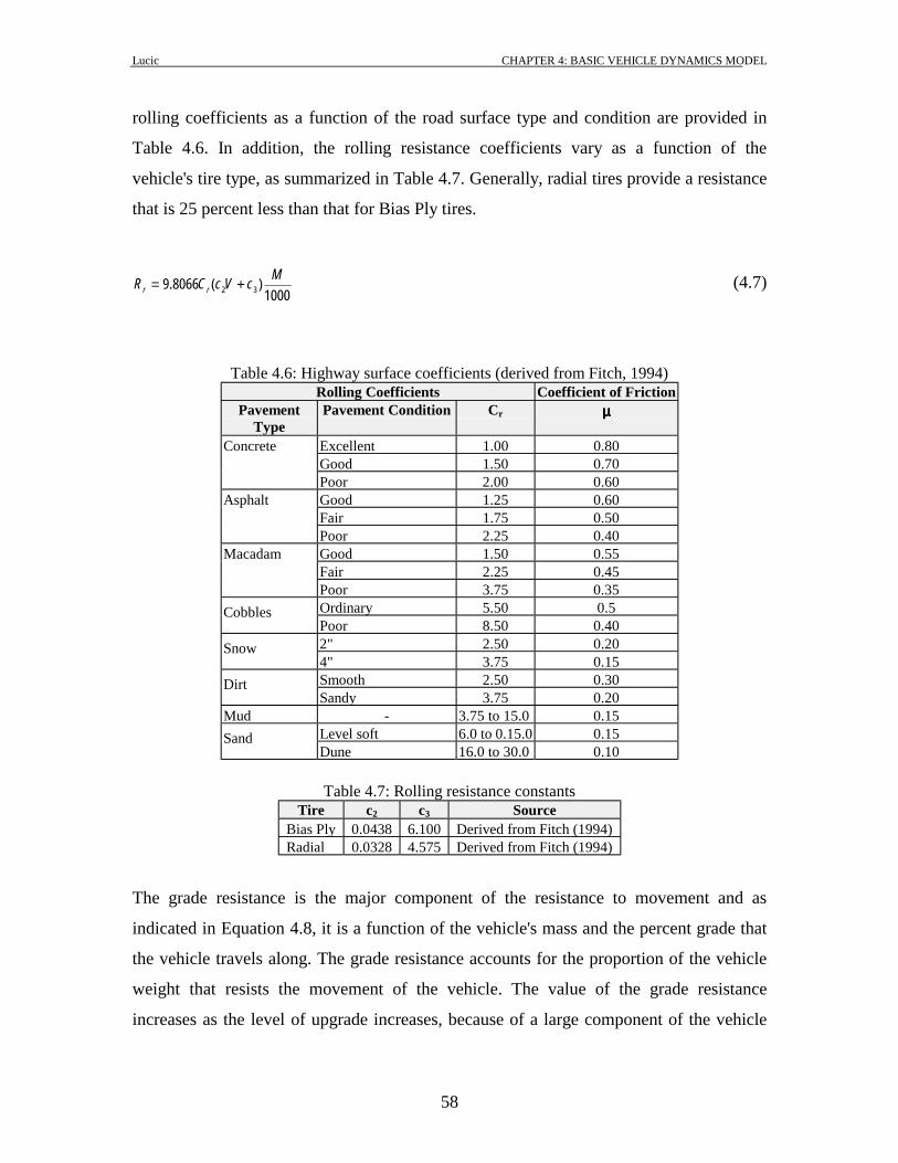
Lucic CHAPTER 4: BASIC VEHICLE DYNAMICS MODEL
58
rolling coefficients as a function of the road surface type and condition are provided in
Table 4.6. In addition, the rolling resistance coefficients vary as a function of the
vehicle's tire type, as summarized in Table 4.7. Generally, radial tires provide a resistance
that is 25 percent less than that for Bias Ply tires.
1000)(8066.9 32
McVcCR rr += (4.7)
Table 4.6: Highway surface coefficients (derived from Fitch, 1994) Rolling Coefficients Coefficient of Friction
Pavement Type
Pavement Condition Cr µµµµ
Excellent 1.00 0.80 Good 1.50 0.70
Concrete
Poor 2.00 0.60 Good 1.25 0.60 Fair 1.75 0.50
Asphalt
Poor 2.25 0.40 Good 1.50 0.55 Fair 2.25 0.45
Macadam
Poor 3.75 0.35 Ordinary 5.50 0.5 Cobbles Poor 8.50 0.40 2" 2.50 0.20 Snow 4" 3.75 0.15 Smooth 2.50 0.30 Dirt Sandy 3.75 0.20
Mud - 3.75 to 15.0 0.15 Level soft 6.0 to 0.15.0 0.15 Sand Dune 16.0 to 30.0 0.10
Table 4.7: Rolling resistance constants
Tire c2 c3 Source Bias Ply 0.0438 6.100 Derived from Fitch (1994) Radial 0.0328 4.575 Derived from Fitch (1994)
The grade resistance is the major component of the resistance to movement and as
indicated in Equation 4.8, it is a function of the vehicle's mass and the percent grade that
the vehicle travels along. The grade resistance accounts for the proportion of the vehicle
weight that resists the movement of the vehicle. The value of the grade resistance
increases as the level of upgrade increases, because of a large component of the vehicle

Lucic CHAPTER 4: BASIC VEHICLE DYNAMICS MODEL
59
weight resists the vehicle’s motion. The larger grade resistance at higher upgrades results
in equilibrium speeds and decrease as a function of the grade magnitude. The equilibrium
speeds represent the speed at which the maximum vehicle acceleration is zero.
MiRg 8066.9= (4.8)
44..33 MMAAXXIIMMUUMM VVEEHHIICCLLEE AACCCCEELLEERRAATTIIOONN
The vehicle acceleration (deceleration) can be expressed as a function of the net force on
the vehicle and using Equation 4.9 it should be possible to compute the maximum vehicle
acceleration. Given that acceleration is the first derivative of speed with respect to time
and that the tractive effort and resistance forces are functions of the vehicle speed,
Equation 4.9 can be solved as an ODE. It should be noted, however, that the variation in
other independent variables including the roadway grade and/or the vehicle power
necessitate solving the ODE numerically.
MRFa −= (4.9)
where a: maximum truck acceleration (m/s2);
F: tractive effort (N);
R: total resistance force (N); and
M: vehicle total mass (kg).
Assuming a constant vehicle power and given that acceleration is the second derivative of
distance with respect to time, Equation 4.9 resolves to a second-order ODE of the form
indicated in Equation 4.10 The ODE is a function of the first derivative of distance
(vehicle speed) because the tractive effort, the rolling resistance, and aerodynamic
resistance forces are all functions of the vehicle speed. In addition, the ODE may be a
function of the distance traveled if the roadway grade changes along the study section. It

Lucic CHAPTER 4: BASIC VEHICLE DYNAMICS MODEL
60
should be noted at this point that because the tractive effort includes a minimum operand,
the derivative of acceleration becomes a non-continuous function. Consequently, a first-
order solution technique is inevitable, as will be described subsequently through thesis.
),( xxfx !!! = (4.10)
Where: x is the distance traveled
44..44 MMOODDEELL VVAALLIIDDAATTIIOONN
In an effort to validate the proposed model together with the recommended input
parameters, a number of field tests were conducted along a test roadway at the VTTI.
This section first describes the test truck that was utilized to conduct the validation effort.
Second, the study roadway section is described in detail prior to discussing the specifics
of the validation effort. Finally, the model validation results are presented and discussed.
4.4.1 Test Truck Characteristics
The test truck that was utilized in the validation effort was a 1990 truck owned by the
VDOT. The truck used a Cummins NTC-350 engine with an engine power rating of 261
kW (350 hp) at an engine speed of 2100 rpm. The peak torque of 1627 N.m (1,200 lbf-ft)
occurred at an engine speed of 1300 rpm. The engine was fairly large with a piston
displacement of 14 liters (850 cu.in); the engine power, however, would be considered
fairly low, as typical truck engines currently range from 223 kW to 485 kW (300 hp to
650 hp).
The test vehicle and trailer was composed of a single trailer with a total of 6 axles, and
thus would be classified as vehicle class 10 using the FHWA classification. The front
axle was a single axle, the tractive axle was a dual axle, and the trailer axle was a triple
axle. The truck did not have any aerodynamic fixtures and used radial tires.

Lucic CHAPTER 4: BASIC VEHICLE DYNAMICS MODEL
61
4.4.2 Study Section Description
The study section that was considered included a 1.5-km (0.9-mi) section of the Smart
Road test facility at the VTTI. Currently, the Smart Road is a 1.5-km (0.9-mi) roadway
that will be expanded to a 3.2-km (2-mi) experimental highway in Southwest Virginia
that spans varied terrain, from in-town to mountain passes.
The horizontal layout of the test section is fairly straight with some minor horizontal
curvature that does not impact vehicle speeds. The vertical layout of the section
demonstrates a substantial upgrade that ranges from 6 percent at the leftmost end to 2.8
percent at the rightmost end, as illustrated in Figure 4.2. In constructing the vertical
profile of the test section the elevation of 35 stations were surveyed, as indicated by the
diamond symbols in Figure 4.2. The vertical profile of the test section was then generated
by interpolating between the station elevations using a cubic spline interpolation
procedure at 1-meter (3.28 ft) increments. The cubic spline interpolation ensures that the
elevations, the slopes, and the rate of change in slopes are identical at the boundary
conditions (in this case every meter). The grade was computed for each 1-meter (3.28 ft)
section and found to vary considerably, as illustrated in Figure 4.2 (thin line). A
polynomial regression relationship was fit to the grade data (R2 of 0.951) for two reasons.
First, to ensure a smooth transition in the roadway grade while maintaining the same
vertical profile. Second, to facilitate the solution of the ODE because it ensures that the
grade function is continuous. The modified grade and vertical elevation, which are
illustrated in Figure 4.2 (thick line), demonstrate an almost identical vertical profile with
much smoother grade transitions when compared to the direct interpolation.
Apart from a 150-m (492-ft) segment of the roadway that was a rigid pavement, the entire
roadway surface was asphalt. Consequently, a rolling resistance coefficient for asphalt
pavement was only utilized. In addition, it should also be noted that the quality of the
road surface was good when the test runs were conducted. These factors are important in
identifying the road surface rolling resistance coefficients, as will be discussed later.

Lucic CHAPTER 4: BASIC VEHICLE DYNAMICS MODEL
62
4.4.3 Test Run Execution In an attempt to validate the dynamics model and the parameters that have been proposed
in the literature, a test truck was driven along the Smart Road test facility. This section
describes how vehicle speeds were measured and the specifics of the test run execution.
The vehicle was equipped with a Global Positioning System (GPS) unit that measured the
vehicle speed to an accuracy of 0.1 m/s (0.305 ft/s). GPS is a worldwide, satellite-based
radio-navigation system that can determine with certain accuracy the position and
velocity of any object equipped with a GPS receiver.
Typical output data from GPS receivers include latitude, longitude, altitude, speed,
heading and time. GPS receivers can also typically update these parameters once every
second. Nominal position accuracy is specified with a 25-m (82-ft) spherical error
probability, while nominal velocity accuracy is specified with a 0.1 m/s (0.31 ft/s) error
probability. These inaccuracies are attributed to a number of sources of error. The
majority of the errors are linked to the way the distance between a satellite and a GPS
receiver is measured. Within the system, distances are measured by calculating the time it
takes for a signal to travel between a satellite and a receiver. Consequently, any delay in
the signal transmission then results in distance overestimation and inaccuracies in the
estimated position of an object.

Lucic CHAPTER 4: BASIC VEHICLE DYNAMICS MODEL
63
-80.398
-80.396
-80.394
-80.392
-80.390
-80.388
-80.386
-80.384
-80.382
37.177 37.178 37.179 37.180 37.181 37.182 37.183 37.184 37.185 37.186 37.187 37.188
Latitude
Long
itude
Section start point
Section end point
590
600
610
620
630
640
650
660
670
680
0 100 200 300 400 500 600 700 800 900 1000 1100 1200 1300 1400 1500Distance (m)
Elev
atio
n (m
)
Interpolated vertical profileSmoothed vertical profileStation locations
0.00
0.01
0.02
0.03
0.04
0.05
0.06
0.07
0 100 200 300 400 500 600 700 800 900 1000 1100 1200 1300 1400 1500Distance (m)
Gra
de
Interpolated grade profileSmoothed grade profile
Figure 4.2: Smart road test section layout

Lucic CHAPTER 4: BASIC VEHICLE DYNAMICS MODEL
64
4.4.4 Test Run Description
The test runs involved accelerating at the maximum possible acceleration rate from a
complete stop at the start of the test section. The acceleration continued until the end of
the test section, over the entire 1.5-km (0.9-mi) section.
In an attempt to alter the mass-to-power ratio, a total of ten mass configurations were
analyzed using the same test truck. The truck and trailer mass was altered by
progressively reducing the number of concrete blocks on the trailer from 9 to 0 blocks,
with each block weighing approximately 2400 kg (5300 lb). Axle weights were recorded
prior to conducting the test runs using General Electrodynamics Corporation (GEC)
weigh scales with an advertised accuracy of 98 percent. In summary, the study involved
varying the mass of the truck and trailer from 22600 to 44800 kg (49880 lb to 98880 lb),
as summarized in Table 4.8, with the mass-to-power ratio varying from 85 kg/kW to 168
kg/kW (140 lb/hp to 277 lb/hp).
Table 4.8: Truck and trailer axle’s mass analyzed Load Configuration Mass (kg) 0 1 2 3 4 5 6 7 8 9 Axle1 4491 4627 4935 4953 5008 5189 4899 5062 5606 5189Axle2 4200 5162 5715 6241 6296 6994 7394 8001 8192 8518Axle3 3865 4672 5352 5842 5869 6523 7040 7575 7865 8083Axle4 3012 3547 4010 4944 5180 5788 5842 7430 8092 8700Axle5 3239 3611 3955 4518 4944 5080 4953 5742 6550 7330Axle6 3856 4336 4518 4817 5126 4790 5080 4935 5625 6985Total 22661 25954 28485 31316 32423 34364 35208 38746 41930 44806
In conducting the study, a minimum of 10 repetitions was executed for each load
configuration in order to provide a sufficient sample size for the validation analysis.
4.4.5 Model Validation Procedures and Results
This section describes how the model and the proposed model parameters were validated
and the results of the validation exercise.
The proposed dynamics model was applied by setting the model parameters to reflect the

Lucic CHAPTER 4: BASIC VEHICLE DYNAMICS MODEL
65
truck, trailer, altitude, tire, and pavement conditions. Values for these parameters were
obtained from the manufacturer’s specifications or from the literature (SAE J2188, 1996;
Fitch, 1994). These parameters included:
a. A horsepower of 261 kW (350 hp), assuming that the engine operates at maximum
power over the entire section (to compute maximum acceleration levels).
b. The percentage mass on the tractive axle was computed as the percentage mass on
axles 2 and 3 relative to the entire truck and trailer mass, as shown in Table 4.9.
c. The power efficiency (η) was set to 0.94 (single drive) as suggested in the literature.
d. The air drag coefficient (Cd) was set to 0.78 because no aerodynamic aids were on the
truck roof.
e. The coefficient of friction (µ) was set to 0.6 and the rolling coefficient (Cr) was set to
1.25 to account for a good asphalt pavement surface.
f. The rolling resistance coefficients were set to 0.04375 and 4.575, respectively to
account for radial tires on the truck and trailer.
g. The frontal area was set to 10.7 m2 (115.2 ft2) for a semi-trailer van type body whose
width is 2.60 m (8.5 ft).
Table 4.9: Model parameters utilized in analysis Weight Configuration 0 1 2 3 4 5 6 7 8 9 Power (HP) 350 350 350 350 350 350 350 350 350 350 Power (kW) 261.1 261.1 261.1 261.1 261.1 261.1 261.1 261.1 261.1 261.1 Mass (kg) 22,208 24,617 27,029 29,440 31,852 34,263 36,675 39,086 41,498 43,910 W/P Ratio (lb/hp) 140 155 170 185 201 216 231 246 261 277 Percta 0.356 0.379 0.389 0.386 0.375 0.393 0.410 0.402 0.383 0.371 Efficiency 0.94 0.94 0.94 0.94 0.94 0.94 0.94 0.94 0.94 0.94 Coeff fric 0.60 0.60 0.60 0.60 0.60 0.60 0.60 0.60 0.60 0.60 Cd 0.78 0.78 0.78 0.78 0.78 0.78 0.78 0.78 0.78 0.78 Ch 0.95 0.95 0.95 0.95 0.95 0.95 0.95 0.95 0.95 0.95 C1 0.04728 0.04728 0.04728 0.04728 0.04728 0.04728 0.04728 0.04728 0.04728 0.04728 C2 0.0328 0.0328 0.0328 0.0328 0.0328 0.0328 0.0328 0.0328 0.0328 0.0328 C3 4.58 4.58 4.58 4.58 4.58 4.58 4.58 4.58 4.58 4.58 Cr 1.25 1.25 1.25 1.25 1.25 1.25 1.25 1.25 1.25 1.25 A (m2) 10.7 10.7 10.7 10.7 10.7 10.7 10.7 10.7 10.7 10.7
Given that the ODE that is presented in Equation 4.11 is a second-order ODE it can be
recast as a system of two first-order equations (an nth-order equation reduces to a set of n

Lucic CHAPTER 4: BASIC VEHICLE DYNAMICS MODEL
66
1st-order equations), as demonstrated in Equation 4.12. These ODEs are solved using a
first-order Euler approximation, as demonstrated in Equations 4.13 and 4.14.
nitittM
tRtFta
i
iii
,...,2,1for:Where
)()()(
0 =∆+=
−= (4.11)
=
)()(
)()(
i
i
i
i
tvta
txtv
!
! (4.12)
ttatvtv iii ∆+= −− )()()( 11 (4.13)
ttvtxtx iii ∆+= −− )()()( 11 (4.14)
where:
∆t = duration of time interval used for solving the ODE (in this case 1-second duration)
F(ti) = total resistance force at instant ti a(ti) = vehicle acceleration at instant ti v(ti) = vehicle speed at instant ti x(ti) = vehicle location along test section at instant ti
Table 4.10 summarizes the solution of the ODE system for nine load configuration for
the first 10 seconds of the trip where
T time (s)
S distance (m)
V speed (km/h)
A acceleration (m/s2)
F force (N)
I grade (%)
Ra air drag resistance (N)
Rr rolling resistance (N)
Rg grade resistance (N)
R total resistance (N)

Lucic CHAPTER 4: BASIC VEHICLE DYNAMICS MODEL
67
It should be noted at this point that a higher order solution to the ODE was not feasible
because the first derivative of the acceleration function was not continuous as explained
earlier. The results for all load configurations are given in Appendix B.
Table 4.10: Example solution to ODE (9-Load Configuration)
T S V a F i Ra Rr Rg R 0 0.00 0.00 0.00 97682 0.0596 0.00 2512.77 26200.14 28712.91 1 0.62 4.98 1.54 97682 0.0596 9.30 2602.56 26201.04 28812.90 2 2.77 10.41 1.25 84854 0.0596 40.61 2700.35 26204.05 28945.02 3 6.20 13.97 0.76 63266 0.0596 73.05 2764.36 26208.54 29045.95 4 10.43 16.34 0.56 54069 0.0597 100.02 2807.16 26213.53 29120.71 5 15.23 18.13 0.44 48723 0.0597 123.17 2839.46 26218.49 29181.12 6 20.47 19.57 0.36 45160 0.0597 143.38 2865.23 26223.04 29231.66 7 26.07 20.75 0.30 42591 0.0597 161.20 2886.50 26226.92 29274.62 8 31.98 21.74 0.25 40642 0.0597 177.03 2904.42 26229.91 29311.35 9 38.14 22.59 0.22 39110 0.0597 191.16 2919.76 26231.83 29342.76
10 44.52 23.33 0.19 37874 0.0597 203.85 2933.04 26232.55 29369.44
The procedures for solving the ODE are best described by illustrating how the various
parameters were computed for the first two seconds of a test run. Using the initial
condition of speed equal to zero (v(t0) = 0), the tractive force, aerodynamic resistance,
and rolling resistance were estimated using Equations 4.1, 4.5, and 4.7. Using the initial
condition of distance equal to zero (x(t0) = 0) the grade was estimated using the
polynomial grade function that was described earlier and the grade resistance was
computed using Equation 4.8. The maximum acceleration was then computed using
Equation 4.9.
At i=1, the speed of the vehicle and location of the vehicle were estimated using
Equations 4.13 and 4.14, respectively using the acceleration at i=0 (t = t0). Again as was
the case at i=0, the tractive force, aerodynamic resistance, rolling resistance, and grade
resistance forces were computed based on: the speed and location after 1 second of travel.
The acceleration at i=1 was then estimated using Equation 4.11.

Lucic CHAPTER 4: BASIC VEHICLE DYNAMICS MODEL
68
The final speed profile from the model was superimposed on the field collected GPS
second-by-second speed measurements, as illustrated in Figure 4.3, which illustrates the
variation in vehicle speed as a function of traveled distance for load configuration 9,
which corresponds to a gross vehicle mass of 44806 kg (98896 lb). The fit indicates a
maximum error in the range of 5 km/h (3.1 mi/h) for the first 200 m (656 ft) with an error
within the variability of the data for 200 m (656 ft) onwards. Figures with generated
curves for all load configurations are given in Appendix B.
0
10
20
30
40
50
60
70
80
90
0 100 200 300 400 500 600 700 800 900 1000 1100 1200 1300 1400 1500Distance (m)
Spee
d (k
m/h
)
Proposed model
Figure 4.3: Predicted and observed speed profile (9-Load Configuration)
The initial error as the truck accelerates from a speed of zero can be explained by the fact
that while the truck initially accelerates the gear shifting behavior results in the vehicle
operating at a power that is less than the maximum power of 261 kW (350 hp). The
analytical model, on the other hand, assumes a constant power of 261 kW (350 hp) over
the entire trip. The dips observed in the measured speed curves are also due to the
shifting of gears, as there is virtually no power transmission to the tractive axles while the
clutch is activated. Further enhancements to the model are being considered to capture
the buildup of power as a vehicle accelerates from a complete stop and to include the
effects of gear shifting that will be described later.

Lucic CHAPTER 4: BASIC VEHICLE DYNAMICS MODEL
69
Similar results are observed for other load configurations. However, only the results for
the configuration 5 and 1 are presented due to lack of space. As illustrated in the other
two graphs shown in Figure 4.4 and Figure 4.5, the error in the estimated speed versus the
measured speed was found to be less than 10 percent at the conclusion of the 1.5-km (0.9-
mi) section. These findings were consistent across the various load configuration tests
and these figures for other load configurations are given in appendix.
0
10
20
30
40
50
60
70
80
90
0 100 200 300 400 500 600 700 800 900 1000 1100 1200 1300 1400 1500Distance (m)
Spee
d (k
m/h
)
Figure 4.4: Predicted and observed speed profile (5-Load Configuration)
0
10
20
30
40
50
60
70
80
90
0 100 200 300 400 500 600 700 800 900 1000 1100 1200 1300 1400 1500Distance (m)
Spee
d (k
m/h
)
Figure 4.5: Predicted and observed speed profile (1-Load Configuration)

Lucic CHAPTER 4: BASIC VEHICLE DYNAMICS MODEL
70
44..55 UUPPDDAATTEEDD SSAAMMPPLLEE PPEERRFFOORRMMAANNCCEE CCUURRVVEESS FFOORR DDEESSIIGGNN TTRRUUCCKK
Having validated the proposed dynamics model, this section demonstrates the model
applicability by developing performance curves for a 120 kg/kW (200 lb/hp) truck along
grades ranging from 0% to 6%, as illustrated in Figure 4.6. These curves can be used to
update the truck performance curves currently used in the geometric design of highways,
among other uses. It should be noted that the performance curves reflect a truck with no
aerodynamic treatments using radial tires driving along a good surfaced asphalt
pavement. Further research is to develop performance curves for different truck and
roadway characteristics and it is done and demonstrated with improvements in the next
chapter.
Figure 4.6 demonstrates that the equilibrium speed for this design truck on a 0% grade is
112 km/h (70 mi/h). Furthermore, the equilibrium speed is very similar for both
acceleration and deceleration curves along a 5-km (16000 ft) section, and identical for
longer sections when the equilibrium speed can be attained. Consequently, these curves
overcome the first shortcoming of the HCM curves, namely the difference in equilibrium
speeds depending on whether the vehicle is accelerating or decelerating. Identical
equilibrium speeds is expected given that the equilibrium speed represents the speed at
which the tractive effort equals the total resistance force, the equilibrium speed is
independent of how the vehicle approaches the equilibrium speed (either accelerating or
decelerating). The updated curves also provide higher equilibrium speeds than proposed
by the HCM curves. For example, the 120 kg/kW (200 lb/hp) test truck has an
equilibrium speed along a 1 percent upgrade slope of 98 km/h (61 mi/h) versus 88 km/h
(55 mi/h) in the HCM. These higher equilibrium speeds are more reflective of the trucks
in North America.
Finally, the model demonstrates a reduction in the equilibrium speed as the vehicle mass-
to-power ratio increases and as the roadway grade increases, as illustrated in Figure 4.7.
Specifically, the equilibrium speed ranges from a high of 120 km/h (70 mi/h) to a low of

Lucic CHAPTER 4: BASIC VEHICLE DYNAMICS MODEL
71
only 30 km/h (19 mi/h) depending on the truck weight-to-power ratio and the roadway
grade.
0
10
20
30
40
50
60
70
80
90
100
110
120
0.0 0.5 1.0 1.5 2.0 2.5 3.0 3.5 4.0 4.5 5.0
Distance (km)
Spee
d (k
m/h
)
Grade = 0%Grade = 1%Grade = 2%Grade = 3%Grade = 4%Grade = 5%Grade = 6%
0
10
20
30
40
50
60
70
80
90
100
110
120
0.0 0.5 1.0 1.5 2.0 2.5 3.0 3.5 4.0 4.5 5.0
Distance (km)
Spee
d (k
m/h
)
Grade = 0%Grade = 1%Grade = 2%Grade = 3%Grade = 4%Grade = 5%Grade = 6%
Figure 4.6: Truck performance curves for NTC-350 engine (200 lb/hp)

Lucic CHAPTER 4: BASIC VEHICLE DYNAMICS MODEL
72
0
20
40
60
80
100
120
140
0.00 0.01 0.02 0.03 0.04 0.05 0.06
Grade
Cra
wl S
peed
(km
/h)
100 lb/hp200 lb/hp300 lb/hp
Figure 4.7: Variation in crawl speed as a function of roadway grade for NTC-350 engine
44..66 CCOONNCCLLUUSSIIOONN
Based on the field tests that were conducted on the Smart Road test facility it can be
concluded that the proposed model and proposed model input parameters provide results
that are consistent with field observations, presenting errors less than 10% and within 5
km/h (3.1 mi/h). The new performance curves could be used to update the curves that are
currently used for the geometric design of highways and climbing lanes.
As in any research effort, further investigations are required to better establish the
accuracy of the proposed models. These investigations will include similar field tests
with alternative trucks to investigate differences in vehicle performance as a function of
engine and truck characteristics as it will be demonstrated in the next chapter. Although,
model will be improved using variable power vehicle dynamic model to give better
results in first 200 m (656 ft) of test field section, where was the maximum error in
comparing model with raw data. The next chapter will provide description, validation,

Lucic CHAPTER 4: BASIC VEHICLE DYNAMICS MODEL
73
and calibration of gearshift model where power is not constant as it was with basic
vehicle dynamics model. Four trucks different performances were used to
validate/calibrate this model.
Lucic CHAPTER 5: VARIABLE POWER VEHICLE DYNAMICS MODEL
74
CHAPTER 5: VARIABLE POWER VEHICLE DYNAMICS MODEL
The chapter five presented the state–of–the-art vehicle dynamics models that can be
utilized to estimate truck speeds. Typical model parameters were introduced and model
speed predictions were compared to field data in an effort to validate the proposed
parameters. Chapter four demonstrated that the constant power assumption that is
inherent results in an overestimation of vehicle speeds at low speed and an under-
estimation at high speeds.
Consequently, this research effort introduces the concept of variable power in order to
enhance current state-of-the-art vehicle dynamics models and capture the build-up of
power as a vehicle engages in gearshifts at low travel speeds. The proposed enhancement
to the current state-of-practice vehicle dynamics model allows the model to reflect typical
vehicle acceleration behavior more accurately. Subsequently, the model parameters are
calibrated using field measurements along a test roadway facility.
55..11 PPRROOPPOOSSEEDD MMOODDEELL EENNHHAANNCCEEMMEENNTT
This section describes the proposed enhancement to the vehicle dynamics model in order
to capture the buildup of power as a vehicle engages in gearshifts. Initially, vehicle
engine characteristics are presented in order to provide a background before describing
the proposed enhancement.
Although a complete description of engine design is beyond the scope of the thesis, an
understanding of how engine output is measured and applied is important to the study of
vehicle performance, which relates to the proposed enhancement to state-of-practice
vehicle dynamics models. The two most commonly used measures of engine output are
torque and power (Mannering and Kilareski, 1990). Specifically, Mannering and

Lucic CHAPTER 5: VARIABLE POWER VEHICLE DYNAMICS MODEL
75
Kilareski (1990) define torque as “the work generated by the engine (the twisting
movement) and is expressed in units of newton-meters (Nm).” In addition, they define
power as “the rate of engine work, usually expressed in kilowatts (kW) for engines,” and
is related to the engine’s torque by Equation 5.1.
10002 TnP π= (5.1)
Where: P Engine power (kW) T Engine torque (Nm) N Engine speed or speed of the crankshaft (revolutions per second)
Figure 5.1 illustrates a sample torque-power diagram for a typical gasoline vehicle
(Oldsmobile Aurora) and a typical diesel engine truck (NTC-350 engine). The figure
clearly demonstrates the differences between an automobile and truck engine. The first
difference is the higher power and torque curves that are associated with truck versus
automobile engines. The second difference is the smaller range of engine speeds for truck
versus automobile engines. Specifically, the engine speed for the Oldsmobile Aurora
extends up to 6200 rpm while the engine speed for the truck extends to 2100 rpm. This
difference signifies the fact that the larger the engine the slower the engine speed of
operation, in order to reduce the significant stresses that build up in the reciprocating
engine parts at high engine speeds. Therefore, most large engines (i.e. engines having a
large bore and stroke) are governed or restricted to a lower engine speed than smaller
bore engines. The third observation from the engine performance curves is that truck
engine curves are typically reported to begin at an engine speed of 1000 to 1200 rpm. The
slowest engine speed at which the engine will operate without stalling or fouling up
averages about 500 to 800 rpm (Fitch, 1994). Typically, an idling engine operates in the
500 to 800 rpm speed range, at which the engine power is zero. Noteworthy from the
figure is that the idle engine speed for the Oldsmobile is approximately 700 rpm with a
power that is approximately 1 percent the maximum power.

Lucic CHAPTER 5: VARIABLE POWER VEHICLE DYNAMICS MODEL
76
The literature also indicates that gear shifting may occur during high idling, which is
illustrated in the figure. The high idling typically occurs at an engine speed that is 100 to
200 rpm above the rated speed and results in an engine power of zero.
Because tractive effort for acceptable vehicle performance is typically higher at lower
vehicle speeds, and because maximum engine torque is developed at fairly high engine
speeds, the use of gasoline-powered engines requires some form of gear reduction. This
gear reduction provides the mechanical advantage necessary for acceptable vehicle
acceleration. With gear reductions, two factors determine the amount of tractive effort
reaching the driving wheels. First, the mechanical efficiency of the driveline (i.e. the gear
reduction devices including the transmission and differential) must be considered, which
typically range between 5 and 25 percent. Second, the overall gear reduction ratio that
refers to the relationship between the revolutions of the engine’s crankshaft and the
revolutions of the road wheels. For example, an overall gear ratio of 4 to 1 means that the
engine’s crankshaft turns four revolutions for every one turn of the road wheel. In order
to illustrate the concept of gear shifting, Figure 5.1 illustrates the torque and power
relationships for the four gears of the Oldsmobile Aurora. Gear shifting typically occurs
at maximum torque, which does not coincide with the maximum power, as demonstrated
in Figure 5.2. Consequently, during gearshifts the vehicle operates at sub-optimal power.
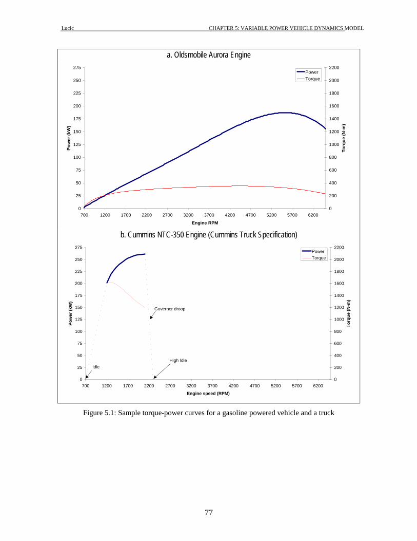
Lucic CHAPTER 5: VARIABLE POWER VEHICLE DYNAMICS MODEL
77
a. Oldsmobile Aurora Engine
0
25
50
75
100
125
150
175
200
225
250
275
700 1200 1700 2200 2700 3200 3700 4200 4700 5200 5700 6200
Engine RPM
Pow
er (k
W)
0
200
400
600
800
1000
1200
1400
1600
1800
2000
2200
Torq
ue (N
-m)
PowerTorque
b. Cummins NTC-350 Engine (Cummins Truck Specification)
0
25
50
75
100
125
150
175
200
225
250
275
700 1200 1700 2200 2700 3200 3700 4200 4700 5200 5700 6200
Engine speed (RPM)
Pow
er (k
W)
0
200
400
600
800
1000
1200
1400
1600
1800
2000
2200
Torq
ue (N
-m)
PowerTorque
High IdleIdle
Governer droop
Figure 5.1: Sample torque-power curves for a gasoline powered vehicle and a truck

Lucic CHAPTER 5: VARIABLE POWER VEHICLE DYNAMICS MODEL
78
0
50
100
150
200
250
300
350
400
0.0 10.0 20.0 30.0 40.0 50.0 60.0 70.0 80.0 90.0 100.0 110.0 120.0 130.0 140.0 150.0 160.0 170.0 180.0 190.0 200.0
Vehicle Speed (km/h)
Torq
ue (N
m)
Gear 1Gear 2Gear 3Gear 4
0102030405060708090
100110120130140150160170180190200
0.0 10.0 20.0 30.0 40.0 50.0 60.0 70.0 80.0 90.0 100.0 110.0 120.0 130.0 140.0 150.0 160.0 170.0 180.0 190.0 200.0
Vehicle Speed (km/h)
Pow
er (k
W)
Gear 1Gear 2Gear 3Gear 4
Figure 5.2: Sample torque and power curves for different gears (Oldsmobile Aurora)

Lucic CHAPTER 5: VARIABLE POWER VEHICLE DYNAMICS MODEL
79
55..22 VVAARRIIAABBLLEE PPOOWWEERR AADDJJUUSSTTMMEENNTT FFAACCTTOORR
While the proposed basic vehicle dynamics model does not involve gear shifting, it does
account for the major behavioral characteristics that result from gear shifting, namely the
reductions of power as gearshifts are being engaged. Specifically, the approach uses a
simple vehicle dynamics model that captures the more complicated gear shifting behavior
while accounting for the buildup of power as a vehicle accelerates from a complete stop.
The modification that is proposed uses a variable power efficiency factor that is
dependent on the vehicle speed, as opposed to the constant factor that is currently utilized
in the model. The factor is a linear relation of vehicle speed with an intercept of zero and
a maximum value of 1.0 at a speed v0, as demonstrated in Equation 5.2. In order to ensure
that the vehicle has sufficient power to accelerate from a speed of zero a vehicle power
lower bound is computed using a speed of 1 km/h, as demonstrated in Equation 5.2. The
adjustment factor is then multiplied by the vehicle power and incorporated in Equation
4.1 to compute the tractive force, as demonstrated in Equation 5.3.
The estimation of the variable power factor “β”requires the calibration of two
parameters, namely, the minimum power and the speed at optimum power. The proposed
model assumes the minimum power to be a function of the optimum speed, as
demonstrated in Equation 5.1. As will be demonstrated in a forthcoming section of the
chapter, these parameters were calibrated using four trucks with vehicle rated powers
ranging from 260 to 375 kW (350 to 500 hp) each involving 10 weight configurations.
The calibration demonstrated that higher weight-to-power ratios required a lower
optimum speed and a higher minimum power. The proposed power lower bound
addresses this need for a variable parameter while maintaining a single calibration
parameter.
Figure 5.3 illustrates the variation in the vehicle power and the resulting vehicle
acceleration by incorporating the power adjustment factor that is presented in Equation

Lucic CHAPTER 5: VARIABLE POWER VEHICLE DYNAMICS MODEL
80
5.1. As illustrated in the figure the modification reduces the vehicle acceleration levels at
the lower speeds while altering acceleration behavior at higher speeds slightly.
The calibration of the variable power factor involves calibrating the speed at which the
vehicle power reaches its maximum (termed the optimum speed). The optimum speed
was found to vary as a function of the weight-to-power ratio, as demonstrated in Figure
5.4. The details of how this relationship was derived is discussed in the model calibration
section, however, it is sufficient to note at this point that the relationship is a power
relationship, as demonstrated by Equation 5.4.
>
≤≤
<
=
0
00
0
0.1
1
11
vv
vvvv
vv
β (5.2)
vPFt β3600= (5.3)
7499.0
0 1164 −= wv (5.4)
Where:
β Variable power factor
v Vehicle speed (km/h) a Calibrated parameter that tends to zero (recommended value
0.01) v0 Speed at which vehicle attains maximum power (km/h) w Vehicle weight-to-power ratio (kg/kW)

Lucic CHAPTER 5: VARIABLE POWER VEHICLE DYNAMICS MODEL
81
0
50
100
150
200
250
300
0 10 20 30 40 50 60 70 80 90 100
Vehicle Speed (km/h)
Vehi
cle
Pow
er (k
W)
Constant PowerVariable Power
0.0
0.5
1.0
1.5
2.0
2.5
0 10 20 30 40 50 60 70 80 90 100
Speed (km/h)
Acc
eler
atio
n (m
/s2 )
Constant PowerVariable Power
Figure 5.3: Variation in vehicle power and acceleration as a function of speed

Lucic CHAPTER 5: VARIABLE POWER VEHICLE DYNAMICS MODEL
82
0
20
40
60
80
100
120
0 20 40 60 80 100 120 140 160 180 200 220 240 260 280 300
Weight/Power Ratio (lb/hp)
350hp Truck430hp Truck470hp Truck500hp Truck
v0 = 1690w-0.7499
R2 = 0.98650
20
40
60
80
100
120
0 20 40 60 80 100 120 140 160 180 200 220 240 260 280 300
Weight-to-power ratio (lb/hp)
0
20
40
60
80
100
120
0 20 40 60 80 100 120 140 160 180 200
Weight/Power Ratio (kg/kW)
260kW Truck320kW Truck350kW Truck375kW Truck
y = 1164x-0.7499
R2 = 0.9888
0
20
40
60
80
100
120
0 20 40 60 80 100 120 140 160 180 200
Weight-to-power ratio (kg/kW)
Figure 5.4: Relationships between speed at optimum power and weight-to-power ratios
The linearly increasing power as a function of vehicle speed in a constant acceleration as
a function of vehicle speed given that force (mass and acceleration) is the first derivative
of power with respect to speed.
Figure 5.5 illustrates the field observed and model predicted vehicle acceleration for the
two load configurations that were illustrated earlier. The figure clearly demonstrates
fluctuations in vehicle accelerations between positive and negative values as the vehicle
engages in initial gearshifts. The trend, however, involves less fluctuations as the vehicle
speed increases. The model predictions appear to reflect the average acceleration
behavior during the initial gear shifting and after the vehicle attains its maximum power.
The acceleration profile as a function of distance also demonstrates consistency between
field data and model predictions, as illustrated in Figure 5.6. The figure also illustrates
that the vehicle attains maximum power within the initial 200 m (656 ft) of travel.

Lucic CHAPTER 5: VARIABLE POWER VEHICLE DYNAMICS MODEL
83
a. 260kW truck with 9 loads
-0.60
-0.40
-0.20
0.00
0.20
0.40
0.60
0.80
1.00
1.20
0.00 10.00 20.00 30.00 40.00 50.00 60.00
Speed (km/h)
Acce
lera
tion
(m/s
2 )
Observed data Model data
b. 260 kW truck with 1 load
-0.60
-0.40
-0.20
0.00
0.20
0.40
0.60
0.80
1.00
1.20
1.40
0.00 10.00 20.00 30.00 40.00 50.00 60.00 70.00 80.00
Speed (km/h)
Acce
lera
tion
(m/s
2 )
Observed data Model data
Figure 5.5: Sample acceleration versus speed profile for 260 kW (350 hp) truck

Lucic CHAPTER 5: VARIABLE POWER VEHICLE DYNAMICS MODEL
84
a. 260kW truck with 9 loads
-0.60
-0.40
-0.20
0.00
0.20
0.40
0.60
0.80
1.00
1.20
0.00 200.00 400.00 600.00 800.00 1000.00 1200.00 1400.00
Distance (m)
Acce
lera
tion
(m/s
2 )Observed data Model data
b. 260 kW truck with 1 load
-0.60
-0.40
-0.20
0.00
0.20
0.40
0.60
0.80
1.00
1.20
1.40
0.00 200.00 400.00 600.00 800.00 1000.00 1200.00 1400.00
Distance (m)
Acce
lera
tion
(m/s
2 )
Observed data Model data
Figure 5.6: Sample acceleration versus distance profile for 260 kW (350 hp) truck

Lucic CHAPTER 5: VARIABLE POWER VEHICLE DYNAMICS MODEL
85
55..33 CCHHAARRAACCTTEERRIIZZAATTIIOONN OOFF TTRRUUCCKKSS OONN UUSS IINNTTEERRSSTTAATTEE HHIIGGHHWWAAYYSS
In order to test the proposed enhanced vehicle dynamics model it was necessary to
calibrate the optimum speed parameter using trucks that cover a typical range of weight-
to-power ratios that are observed in the field. This section describes the characterization
of in-field trucks that was necessary for the calibration effort.
The characterization of trucks along interstate highways was achieved by conducting a
one-day survey at the Troutville weigh station along Interstate 81 was described in
Chapter 3. Specifically, a random sample of about 200 trucks was included in the survey,
of which 157 were classified as vehicle class 9. Figure 5.7 clearly demonstrates that the
distribution of truck weights for the sample that was included in the survey was very
similar to typical truck weight distributions along I-81.
In conducting the survey, the weights of the sample trucks were obtained from the static
scales at the weigh station. In addition, information on the engine power, type of tires,
aerodynamic features, and type of transmission were obtained through a questionnaire
that was conducted with the truck drivers as was explained in Chapter 3.
The weight of the trucks ranged from 6800 kg (10000 lbs) to 38000kg (90000 lbs), as
illustrated in Figure 5.7. The truck powers ranged from a minimum of 150 kW (200 hp)
to a maximum of 450 kW (600 hp) with the majority of trucks falling in the 260 kW (350
hp) to 415 kW (550 hp) range (82 percent of the truck sample). The average truck power
was 325 kW (435 hp) with a standard deviation of 55 kW (70 hp). Consequently, the 95%
confidence limits ranged from 225 kW (300hp) to a 430 kW (575hp). The weight-to-
power ratio for the sample ranged from a minimum of 25 kg/kW (44 lb/hp) to a
maximum of 150 kg/kW (240 lb/hp) with a mean of 80 kg/kW (130 lb/hp) and a standard
deviation of 25 kg/kW (45 lb/hp). Consequently, the 95% confidence limits ranged from
approximately 30 to 130 kg/kW (40 to 220 lb/hp).

Lucic CHAPTER 5: VARIABLE POWER VEHICLE DYNAMICS MODEL
86
0%
10%
20%
30%
40%
Truck Weight (lb)
Freq
uenc
y
Friday Avg. 0% 5% 5% 16% 14% 20% 14% 24% 2%Survey 0% 1% 6% 21% 11% 18% 10% 31% 1%
10000 20000 30000 40000 50000 60000 70000 80000 90000
0%
10%
20%
30%
40%
Truck Weight (kg)
Freq
uenc
y
Friday Avg. 0% 5% 5% 16% 14% 20% 14% 24% 2%Survey 0% 1% 6% 21% 11% 18% 10% 31% 1%
2268 6804 11340 15876 20412 24947 29483 34019 38555
0%
5%
10%
15%
20%
25%
30%
35%
Truck Power (hp)
Freq
uenc
y
Survey 0% 1% 4% 11% 13% 29% 32% 8% 1% 0%200 250 300 350 400 450 500 550 600 650
0%
5%
10%
15%
20%
25%
30%
35%
Truck Power (kW)
Freq
uenc
y
Survey 0% 1% 4% 11% 13% 29% 32% 8% 1% 0%
149 187 224 261 298 336 373 410 448 485
0%
5%
10%
15%
20%
25%
Weight-to-Power Ratio (lb/hp)
Freq
uenc
y
Survey 0% 1% 12% 20% 12% 20% 20% 10% 4% 1% 0%25 50 75 100 125 150 175 200 225 250 275
0%
5%
10%
15%
20%
25%
Weight-to-Power Ratio (lb/hp)
Freq
uenc
y
Survey 0% 1% 12% 20% 12% 20% 20% 10% 4% 1% 0%15 30 46 61 76 91 106 122 137 152 167
Figure 5:7: Truck characterization at I-81 Troutville weigh station

Lucic CHAPTER 5: VARIABLE POWER VEHICLE DYNAMICS MODEL
87
55..44 MMOODDEELL CCAALLIIBBRRAATTIIOONN
Having characterized the trucks along typical I-81, the next step was to calibrate the
proposed enhanced model parameters for trucks that travel along US highways. This
section describes how the optimum speed was calibrated using four trucks with different
weight configurations. The characteristics of the trucks are summarized in Table 5.1.
Each of these four trucks was tested for at least 10 weight configurations along the Smart
Road test facility, as summarized in Table 5.2. In addition, two of the trucks were tested
without a trailer in order to cover the fairly low weight-to-power ratios that were
observed in the field. The test scenarios covered a range of weight-to-power ratios from
24 kg/kW to 171 kg/kW (39 lb/hp to 282 lb/hp), weight ratios from 8373 kg (18460 lb) to
44806 kg (98780 lb), and both ranges cover data that were observed in the field. The
truck powers ranged from a minimum of 260 kW (350 hp) to a maximum of 375 kW
(500 hp), which does not cover the full range of the sample that was observed in the field
but does cover a substantial range (85 percent of the field observations). It should also be
noted that the trucks included engines that were developed by different engine
manufacturers for different model years. All trucks were equipped with radial tires and all
trucks were manual, which is consistent with the survey data that were gathered.
Table 5.1: Test truck characteristics
260-kW (350-hp)
320-kW (430-hp)
350-kW (470-hp)
375-kW (500-hp)
Vehicle year 1990 1998 1997 1997 Engine manufacturer Cummins Detroit Diesel Detroit Diesel Detroit Diesel Engine power 260 320 350 375 Engine RPM 2100 1800 2100 2100 Number of gears 9 10 10 10 Aerodynamic features None Full Full Full
The execution of the test runs was identical to what was described previously in Chapter
4 where drivers accelerated from a full stop at the maximum possible rate as they traveled
along the test roadway. The model parameters were selected based on recommendations
in Chapter 4 to reflect the characteristics of the trucks. Multiple repetitions were made for
each weight-to-power ratio combination in order to ensure that the runs were not biased

Lucic CHAPTER 5: VARIABLE POWER VEHICLE DYNAMICS MODEL
88
by a single observation. The test scenarios included a total of 42 weight-to-power
combinations, as summarized in Table 5.1. For each scenario the system of two first-
order ODEs was solved using a first-order Euler approximation that was presented earlier
in Equations 4.13 and 4.14.
Table 5.2: Truck weight-to-power experimental design (kg/kW)
Test Truck Breaking Power Load Configuration 260-kW (350-hp) 320-kW (430-hp) 350-kW (470-hp) 375-kW (500-hp)
No Trailer 27 24 Trailer no load 87 64 64 61 Trailer 1 load 96 78 72 67 Trailer 2 loads 106 86 80 74 Trailer 3 loads 115 92 88 80 Trailer 4 loads 125 100 92 87 Trailer 5 loads 134 108 101 94 Trailer 6 loads 143 112 106 100 Trailer 7 loads 153 121 112 107 Trailer 8 loads 162 127 118 114 Trailer 9 loads 171 134 126 120
The estimation of the optimum speed for each weight-to-power scenario was computed
by solving a constrained non-linear optimization problem, as demonstrated in Equation
5.5. The objective function is to minimize the sum of squared error between the estimated
and observed speeds for each observation j. The constraints ensure that the estimated
speeds and distances traveled satisfy the system of first-order ODEs in addition to the
non-negativity constraints.
( )
0)(~),(~)(~)(~)(~
)(~)(~)(~S.T.
~min
11
11
2
1
≥∆+=
∆+=
−=
−−
−−
=∑
ii
iii
iii
n
jxx
tvtxttvtxtx
ttatvtv
vvEjj
(5.5)
Where:
jxv Observed speed at the distance location of observation j
jxv~ Estimated speed at the distance location of observation j

Lucic CHAPTER 5: VARIABLE POWER VEHICLE DYNAMICS MODEL
89
The calibrated optimum speed was found to decrease as a function of the weight-to-
power ratio in a consistent fashion for the various trucks, as illustrated in Figure 5.4. A
regression model was fit to the 42 observations to generate the relationship between the
optimum speed and the weight-to-power ratio, as indicated in Equation 5.4.
Figure 5.8 and Figure 5.9 illustrate for the same sample runs the model predicted truck
speed profile based on the constant power and variable power vehicle dynamic models. In
addition, Table 5.3 and Table 5.4 summarize the solution of the ODE system for the
sample nine and single load configurations by applying the variable vehicle dynamic
model for the first 10 seconds of the trip.
Solutions for the same truck using the constant power vehicle dynamics model was
provided earlier in Chapter 4. The results for both models for all load configurations and
all trucks are given in Appendix B.
Comparing Figure 5.8 and Figure 5.9 clearly demonstrates an improvement in vehicle
speed predictions as a result of introducing the variable power concept. Findings are
observed for the other 40 weight-to-power combinations that were tested, as illustrated in
Appendix B.
Table 5.3: Example solution to ODE (9-Load Configuration) T S V a F i Ra Rr Rg R
0 0.00 0.00 0.00 39165 0.0596 0.0 2512.8 26200.1 28712.9 1 0.00 0.00 0.23 39165 0.0596 0.0 2512.8 26200.1 28712.9 2 0.00 0.84 0.23 39165 0.0596 0.3 2527.9 26200.1 28728.3 3 0.23 1.68 0.23 39165 0.0596 1.1 2543.0 26200.5 28744.5 4 0.70 2.52 0.23 39165 0.0596 2.4 2558.1 26201.2 28761.6 5 1.40 3.35 0.23 39165 0.0596 4.2 2573.1 26202.1 28779.5 6 2.33 4.19 0.23 39165 0.0596 6.6 2588.2 26203.4 28798.2 7 3.49 5.02 0.23 39165 0.0596 9.4 2603.2 26205.0 28817.6 8 4.89 5.85 0.23 39165 0.0596 12.8 2618.2 26206.9 28837.8 9 6.51 6.68 0.23 39165 0.0596 16.7 2633.1 26208.9 28858.7
10 8.37 7.51 0.23 39165 0.0597 21.1 2648.0 26211.2 28880.3

Lucic CHAPTER 5: VARIABLE POWER VEHICLE DYNAMICS MODEL
90
Table 5.4: Example solution to ODE (1-Load Configuration) T S V a F i Ra Rr Rg R
0 0.00 0.00 0.00 24736 0.0596 0.0 1408.8 14688.8 16097.6 1 0.00 0.00 0.34 24736 0.0596 0.0 1408.8 14688.8 16097.6 2 0.00 1.24 0.34 24736 0.0596 0.6 1421.3 14688.8 16110.7 3 0.34 2.47 0.34 24736 0.0596 2.3 1433.7 14689.1 16125.2 4 1.03 3.71 0.34 24736 0.0596 5.1 1446.2 14689.7 16141.0 5 2.06 4.94 0.34 24736 0.0596 9.1 1458.6 14690.5 16158.3 6 3.43 6.17 0.34 24736 0.0596 14.3 1471.1 14691.5 16176.9 7 5.15 7.40 0.34 24736 0.0596 20.5 1483.5 14692.8 16196.7 8 7.20 8.62 0.34 24736 0.0597 27.8 1495.8 14694.2 16217.9 9 9.60 9.84 0.34 24736 0.0597 36.3 1508.1 14695.8 16240.2
10 12.33 11.06 0.34 24736 0.0597 45.8 1520.4 14697.5 16263.7
Additionally, a Matlab computer program was used to estimate optimum vehicle speeds
and the error in speed along the test section traveled for both models that are already
demonstrated. Program makes best fit for observed data using polynomial function and
Figures for sample speed profiles are given with Figure 5.10. Error in speed difference
along test section was computed for each meter and curves for sample speed profiles for
observed data and both models are shown with Figure 5.11. Optimum vehicle speeds are
summarized in Table 5.5 and code for a sample 260 kW (350 hp) truck with no loads is
given in Appendix C. Figure 5.12 illustrates comparison of error in speeds versus
distance traveled for both models and for sample runs already mentioned. Figures with
error curves for all load configurations are shown in Appendix C. Mean square errors
were computed and summarized for both models in Table 5.6 and Table 5.7. These tables
show that variable power vehicle dynamic model gives much better results than using
constant power vehicle dynamic model.
Figure 5.13 and Figure 5.14 illustrate for the truck runs without trailer estimating the
truck speed profile using both models constant power vehicle dynamic model and
variable power vehicle dynamic model and for truck with 350 kW (470 hp). Computed
mean square errors for these two cases and for both models are bigger comparing with
other load configurations. Reason for that problem for constant vehicle dynamics model
lie in the first 200 m (656 ft) where gearshift was problem to accelerate more in order to
produce higher speed and looking at curves generated from both models. The last 300 m

Lucic CHAPTER 5: VARIABLE POWER VEHICLE DYNAMICS MODEL
91
(984 ft) shows overestimating and reason for that is safety. At the end of the test section
there is a loop and trucks produced very high speed that was not possible to stop safely.
Drivers reduced the speed before the end of the section.
a. 260kW truck with 9 loads
0
10
20
30
40
50
60
70
80
90
0 100 200 300 400 500 600 700 800 900 1000 1100 1200 1300 1400 1500
Distance (m)
Spee
d (k
m/h
)
b. 260 kW truck with 1 load
0
10
20
30
40
50
60
70
80
90
0 100 200 300 400 500 600 700 800 900 1000 1100 1200 1300 1400 1500
Distance (m)
Spee
d (k
m/h
)
Figure 5.8: Sample speed profile validation using the constant power model (NTC-350 engine)

Lucic CHAPTER 5: VARIABLE POWER VEHICLE DYNAMICS MODEL
92
a. 260kW truck with 9 loads
0
10
20
30
40
50
60
70
80
90
0 100 200 300 400 500 600 700 800 900 1000 1100 1200 1300 1400 1500
Distance (m)
Spee
d (k
m/h
)
b. 260 kW truck with 1 load
0
10
20
30
40
50
60
70
80
90
0 100 200 300 400 500 600 700 800 900 1000 1100 1200 1300 1400 1500
Distance (m)
Spee
d (k
m/h
)
Figure 5.9: Sample speed profile validation using the variable power model
(NTC-350 engine)

Lucic CHAPTER 5: VARIABLE POWER VEHICLE DYNAMICS MODEL
93
a. 260kW truck with 9 loads
0
10
20
30
40
50
60
70
80
90
0 100 200 300 400 500 600 700 800 900 1000 1100 1200 1300 1400 1500
Distance (m)
The best fit from observed data
b. 260 kW truck with 1 load
0
10
20
30
40
50
60
70
80
90
0 100 200 300 400 500 600 700 800 900 1000 1100 1200 1300 1400 1500
Distance (m)
Figure 5.10: Sample speed profile with the best fit used for error computing (NTC-350 engine)

Lucic CHAPTER 5: VARIABLE POWER VEHICLE DYNAMICS MODEL
94
a. 260kW truck with 9 loads
0
5
10
15
20
25
30
35
40
45
50
55
0 100 200 300 400 500 600 700 800 900 1000 1100 1200 1300 1400 1500
Distance (m)
Spee
d (k
m/h
)Observed data Constant model Variable model
b. 260 kW truck with 1 load
0
5
10
15
20
25
30
35
40
45
50
55
60
65
70
75
80
0 100 200 300 400 500 600 700 800 900 1000 1100 1200 1300 1400 1500
Distance (m)
Spee
d (k
m/h
)
Observed data Constant model Variable model
Figure 5.11: Sample speed profile comparing observed data with both models (NTC-350 engine)

Lucic CHAPTER 5: VARIABLE POWER VEHICLE DYNAMICS MODEL
95
a. 260kW truck with 9 loads
-6
-4
-2
0
2
4
6
8
10
0 200 400 600 800 1000 1200 1400
Distance (m)
Erro
r (km
/h)
Constant Power Model Variable Power Model
b. 260 kW truck with 1 load
-6
-4
-2
0
2
4
6
8
10
12
14
0 200 400 600 800 1000 1200 1400
Distance (m)
Erro
r (km
/h)
Constant Power Model Variable Power Model
Figure 5.12: Comparison of error versus distance traveled for constant and variable power vehicle dynamic models
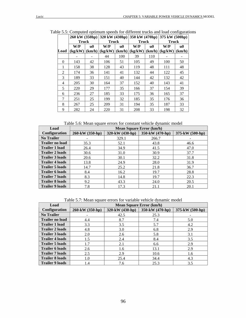
Lucic CHAPTER 5: VARIABLE POWER VEHICLE DYNAMICS MODEL
96
Table 5.5: Computed optimum speeds for different trucks and load configurations 260 kW (350hp)
Truck 320 kW (430hp)
Truck 350 kW (470hp)
Truck 375 kW (500hp)
Truck
Load W/P
(kg/kW) u0
(km/h) W/P
(kg/kW) u0
(km/h) W/P
(kg/kW) u0
(km/h) W/P
(kg/kW) u0
(km/h) - - 44 100 39 110 - -
0 143 42 106 51 105 49 100 50 1 158 38 128 43 119 48 111 48 2 174 36 141 41 132 44 122 45 3 189 33 151 40 144 42 132 42 4 205 30 164 37 152 40 143 41 5 220 29 177 35 166 37 154 39 6 236 27 185 33 175 36 165 37 7 251 25 199 32 185 35 176 36 8 267 25 209 31 194 35 187 33 9 282 24 220 31 208 33 198 32
Table 5.6: Mean square errors for constant vehicle dynamic model Mean Square Error (km/h) Load
Configuration 260-kW (350-hp) 320-kW (430-hp) 350-kW (470-hp) 375-kW (500-hp) No Trailer - 329.1 266.7 - Trailer no load 35.3 52.1 43.8 46.6 Trailer 1 load 26.4 34.9 41.5 47.0 Trailer 2 loads 30.6 31.0 30.9 37.7 Trailer 3 loads 20.6 30.1 32.2 31.8 Trailer 4 loads 13.8 24.9 28.0 31.9 Trailer 5 loads 14.7 25.2 21.8 36.7 Trailer 6 loads 8.4 16.2 19.7 28.8 Trailer 7 loads 8.3 14.8 19.7 22.3 Trailer 8 loads 9.2 43.3 24.0 20.5 Trailer 9 loads 7.8 17.3 21.1 20.1
Table 5.7: Mean square errors for variable vehicle dynamic model Mean Square Error (km/h) Load
Configuration 260-kW (350-hp) 320-kW (430-hp) 350-kW (470-hp) 375-kW (500-hp) No Trailer - 42.5 25.3 - Trailer no load 4.4 8.7 7.4 5.0 Trailer 1 load 3.3 3.5 5.7 4.2 Trailer 2 loads 4.8 3.0 6.8 2.9 Trailer 3 loads 2.0 2.6 5.8 3.1 Trailer 4 loads 1.5 2.4 8.4 3.5 Trailer 5 loads 1.7 2.1 6.6 2.9 Trailer 6 loads 2.6 1.6 13.1 2.9 Trailer 7 loads 2.5 2.9 10.6 1.6 Trailer 8 loads 1.0 25.4 34.4 4.3 Trailer 9 loads 1.4 7.6 25.3 3.5

Lucic CHAPTER 5: VARIABLE POWER VEHICLE DYNAMICS MODEL
97
a. 350kW truck without trailer
0102030405060708090
100110120130140
0 100 200 300 400 500 600 700 800 900 1000 1100 1200 1300 1400 1500
Distance (m)
b. 350 kW truck without trailer
0
20
40
60
80
100
120
140
0 100 200 300 400 500 600 700 800 900 1000 1100 1200 1300 1400 1500
Distance (m )
Figure 5.13: Sample speed profile validation using the constant power model (470 hp engine)

Lucic CHAPTER 5: VARIABLE POWER VEHICLE DYNAMICS MODEL
98
a. 350kW truck without trailer
0102030405060708090
100110120130140
0 100 200 300 400 500 600 700 800 900 1000 1100 1200 1300 1400 1500
Distance (m)
b. 350 kW truck without trailer
0
20
40
60
80
100
120
140
160
0 100 200 300 400 500 600 700 800 900 1000 1100 1200 1300 1400 1500
Distance (m )
Figure 5.14: Sample speed profile validation using the variable power model (470 hp engine)
Variable power vehicle dynamics model has better results than basic vehicle dynamics
model and performance curves for sample 261 kW (350 hp) truck should be updated. Figure 5.15 illustrates acceleration and deceleration performance curves for design truck
with weight-to-power ratio of 120 kg/kW (200 lb/hp) comparing HCM curves and those

Lucic CHAPTER 5: VARIABLE POWER VEHICLE DYNAMICS MODEL
99
generated from the model. Figure clearly demonstrates difference between HCM curves
and curves from the model. Differences in equilibrium speeds are in a range of 12 km/h.
0102030405060708090
100110120
0.0 0.5 1.0 1.5 2.0 2.5 3.0 3.5 4.0 4.5 5.0Distance (km)
Spee
d (k
m/h
)
Model = 1% Model = 2% Model = 3%Model = 4% Model = 5% Model = 6%HCM = 1% HCM = 2% HCM = 3%HCM = 4% HCM = 5% HCM = 6%
Truck acceleration performance
0102030405060708090
100110120
0.0 0.5 1.0 1.5 2.0 2.5 3.0 3.5 4.0 4.5 5.0Distance (km)
Spee
d (k
m/h
)
Model = 1% Model = 2% Model = 3%Model = 4% Model = 5% Model = 6%HCM = 1% HCM = 2% HCM = 3%HCM = 4% HCM = 5% HCM = 6%
Truck deceleration performance
Figure 5.15: Truck performance curves for NTC-350 engine (200 lb/hp)

Lucic CHAPTER 5: VARIABLE POWER VEHICLE DYNAMICS MODEL
100
55..55 CCOONNCCLLUUSSIIOONN
In summary, the chapter introduced the concept of a linearly increasing variable power to
the basic vehicle dynamics model. The chapter also presented calibration of the model to
typical trucks that travel along interstate highways in the US. The proposed enhancement
resulted in significant improvements in vehicle performance curves especially at low
speeds when vehicles are engaged in gearshifts. Computed errors for both presented
models show that variable power vehicle dynamics model has much better results. Table
5.8 summarizes percentage in error difference for these two models. The truck power of
350 kW (470 hp) had general problem with gearshift and that is reason for lower
difference than for other trucks. The biggest problem was utilizing truck with 8 and 9
load configurations.
Table 5.8: Difference in error computed for both models Error difference in percent Load
Configuration 260-kW (350-hp)
320-kW (430-hp)
350-kW (470-hp)
375-kW (500-hp)
No Trailer - 87.1 90.5 - Trailer no load 87.5 83.3 83.1 89.3 Trailer 1 load 87.5 90.0 86.3 91.1 Trailer 2 loads 84.3 90.3 78.0 92.3 Trailer 3 loads 90.3 91.4 82.0 90.3 Trailer 4 loads 89.1 90.4 70.0 89.0 Trailer 5 loads 88.4 91.7 69.7 92.1 Trailer 6 loads 69.0 90.1 33.5 89.9 Trailer 7 loads 69.9 80.4 46.2 92.8 Trailer 8 loads 89.1 41.3 -43.3 79.0 Trailer 9 loads 82.1 56.1 -19.9 82.6
Lucic CHAPTER 6: CONCLUSIONS AND RECCOMENDATION
101
CHAPTER 6: CONCLUSIONS AND RECCOMENDATION
The thesis attempted to develop models that can be utilized to quantify the impact of
trucks on roadway operations. A first step in developing these models was to characterize
the trucks that travel on US interstate highways. Next, the thesis introduced the concept
of a linearly increasing power to the basic vehicle dynamics model that has been
proposed in the literature. The proposed enhancement was found to produce significant
improvements in the state-of-the-art vehicle dynamic model especially at low speeds
when vehicles engage in gearshifts. This chapter summarizes the main contributions,
findings, and conclusions of the thesis. In addition, recommendations for further research
are presented.
66..11 PPRROOBBLLEEMM OOVVEERRVVIIEEWW
Heavy vehicles play an important role in ground transportation in the US. They have
significant impacts on traffic, because of their characteristics, size, weights, and ability to
accelerate/decelerate. The percentage of trucks on US interstate highways is significant.
For example, on I–81 approximately 40% of the average daily traffic are trucks. Truck
performance along grade sections may have significant impacts on roadway throughput
depending on the grade level, the truck characteristics, the percentage of trucks, and the
level of congestion along the roadway section. Every year truck technology has some
innovations and their characterization and classification on US roads is essential.
The HCM provides curves for predicting vehicle speeds as a function of the distance
traveled and the percentage grade along the section (TRB, 1997), these curves were
developed several decades ago and thus may not be representative of current trucks.
Furthermore, the curves do not capture the effect of other factors on vehicle performance
like for example the availability of aerodynamic aids and the type of pavement

Lucic CHAPTER 6: CONCLUSIONS AND RECCOMENDATION
102
66..22 TTHHEESSIISS SSUUMMMMAARRYY
State-of-the-art vehicle dynamics models were validated along the Smart Road test
facility for typical truck characteristics. It was found that these models overestimated
vehicle speeds at low speeds and typically under-estimated the vehicle speeds at the high
speeds. The test runs involved accelerating at the maximum possible acceleration rate
from a complete stop at the start of the test section. The acceleration continued until the
end of the test section, over the entire 1.5-km (0.9-mi) section. Four trucks were utilized
with a trailer for 10 weight-to-power configurations. The proposed dynamics model was
applied by setting the model parameters to reflect the truck, trailer, altitude, tire, and
pavement conditions. Values for these parameters were obtained from the manufacturer’s
specifications or from the literature (SAE J2188, 1996; Fitch, 1994).
The calibration of the model require calibrating a single parameter which was conducted
using four trucks with ten weight configurations resulting in a total of 42 weigh-to-power
configurations.
66..33 TTHHEESSIISS CCOONNTTRRIIBBUUTTIIOONNSS
The thesis makes four significant contributions, which are the follows:
1. The thesis attempts to characterize trucks traveling along US highways by
analyzing data from Interstate 81. I-81 is a typical of US highways and thus can
provide some insight into typical truck characteristics. These truck characteristics
are important for the development of an exhaustive vehicle performance
procedure.
2. The thesis collects a database of systematic field data that can be utilized for the
validation of vehicle performance models. This database is unique because it was
conducted in a controlled field environment where the vehicle is only constrained
by its dynamics.

Lucic CHAPTER 6: CONCLUSIONS AND RECCOMENDATION
103
3. The thesis validates a state-of-the-art constant power vehicle dynamics model that
has been presented in the literature using field data that were collected along the
Smart Road test facility. In addition the thesis identifies typical input parameters
and validates these parameters against field measurements.
4. The thesis extends the vehicle dynamics model by introducing the concept of
variable power in order to capture the buildup of power as the vehicle engages in
gearshifts. The proposed enhancement results in a significant enhancement to the
current state-of-the-art vehicle dynamics model.
66..44 TTHHEESSIISS CCOONNCCLLUUSSIIOONNSS
Data analysis of the truck data on the I-81 corridor indicated that the majority of trucks
could be classified as vehicle class 9 (84.3% in 1998, 91.2% in 1999, and 86.6% in 2000
year). The heaviest day-of-week demand occurred on Thursdays and Wednesdays for
both directions of travel (between 12% and 20% of total demand). The frequency
distribution of weights was not found to follow either a normal or log-normal
distribution.
The single day survey indicated that the average vehicle mass was 35380 kg (77836 lb),
the most frequent engine power ranged from 335 kW (450 hp) to 375 kW (500 hp), and
the weight-to-power ration ranged from 55 kW/kg (90 lb/hp) to 115 kW/kg (190 lb/hp).
In terms of validating the vehicle dynamic model, the following conclusions can be
made:
1. The model parameters that are suggested in the literature and summarized in
Chapter 4 are consistent with field measurements.
2. The use of a constant transmission efficiency results in an over-estimation of
vehicle speeds at low speeds and an under-estimation at high speeds.

Lucic CHAPTER 6: CONCLUSIONS AND RECCOMENDATION
104
3. The proposed linear power relationship provides a good fit to field data over the
full range of vehicle speeds (error less than 10%).
66..55 FFUUTTUURREE RREESSEEAARRCCHH
It is recommended that further research be conducted in calibrating similar power
relationships for other vehicle classes including automobiles, buses, and smaller trucks.
As in any research effort, further investigations are required to better establish the
accuracy of the proposed models. These investigations will include:
1. Conduct similar field tests to establish the sensitivity of truck performance to type
of pavement, to pavement condition, to type of vehicle tires, and to percentage
weight on the tractive axle;
2. It is recommended that further research be conducted in calibrating similar power
relationships for other vehicle classes including automobiles, buses, and smaller
trucks;
3. Develop curves similar to the HCM curves that reflect grade, truck, pavement,
and tire conditions; and
4. Incorporate the proposed model within a microscopic simulation software to
evaluate the impact of trucks on system throughput for different roadway, traffic,
and pavement characteristics.

Lucic REFERENCES
105
REFERENCES
1. Archilla A. R. and De Cieza A. O. F., ‘Truck Performance on Argentinean
Highways’, Transportation Research Record, n 1555, Nov 1996, p 114-123
2. A.M. Khan, J. Y. Wong, and M. Rastogi, ‘Heavy Vehicle Performance on Grade
and Climbing Lane Criteria’, Final Report of Research and Development Project
3. A.T. Papagiannakis, W. A. Phang, J. H. F. Woodrooffe, A. T. Bergan, and R. C.
G. Hass, ‘Accuracy of Weigh-in-motion Scales and Piezoelectric Cables’,
Transportation Research Record 1215, 1989
4. Bahman Izadmehr and Clyde E. Lee, ‘On-Site Calibration of Weigh-in-motion
Systems’, Transportation Research Record n 1123, 1989, pp 136-144
5. Bahman Izadmehr and Clyde E. Lee, ‘Accuracy and Tolerances of Weigh-in-
motion Systems’, Transportation Research Record 1123, 1989, pp 127-135
6. Barton, Raymond A. Morrall, John, ‘Study of long combination vehicles on two-
lane highways’, Transportation Research Record. n 1613 Aug 1998. p 43-49
7. Bruce G. Hutchinson, ‘Large-Truck Properties and Highway Design Criteria’,
Journal of Transportation Engineering, Vol. 116, No. 1, January, 1990
8. Chia-pei J. Chou and Chung-piau Ching, ‘Truck Load Distribution and Its
Impacts on Vehicle Weight Regulations in Taiwan’, Transportation Research
Record 1501, 1995
9. D. W. Lear, M. Bettison, and G. Kent, ‘Advances in Piezoelectric Axle Sensor
Design’, Transport and Road Research Laboratory, V. 30, n. 1, Jan 1989
10. Edward S. K. Fekpe, ‘Characteristics of Heavy Vehicle Weight Distributions and
Pavement Loading’, PhD Thesis, Department of Civil Engineering, University of
Manitoba, Winnipeg, Canada, 1993
11. Edward S. K. Fekpe and A. M. Clayton, ‘Vehicle Clasification from Weigh-in-
motion Data: The Progressive Sieving algorithm’, Canadian Journal of Civil
Engineers 21, 1994, pp 195-206
12. Edward S. K. Fekpe, ‘Utilisation of five- and six-axle Tractor Semitrailers in
Western Canada’, Heavy Vehicle Systems, Vol. 4, No. 1, 1997.

Lucic REFERENCES
106
13. Edward S. K. Fekpe, Alan M. Clayton, and Attahiru Sule Alfa, ‘Aspects of
Performance of Truck Weigh Stations’, Canadian Journal of Civil Engineering 20,
1993, pp 380-385
14. Edward S. K. Fekpe and Alan Clayton, ‘Prediction of Heavy-Vehicle Weight
Distributions’, Journal of Transportation Engineering, v121, n2, Mar-Apr 1995,
pp 158-168
15. ERES Consultants and Fugro-Bre, ‘Determination of Traffic Information and
Data for Pavement Structural Design and Evaluation’, National Cooperative
Highway Research program, Transportation research Board, National Research
Council, December, 1999
16. ERES Consultants and Fugro-Bre, ‘Traffic Input Guide’, National Cooperative
Highway Research program, Transportation research Board, National Research
Council, January, 2000
17. Fitch J. W., ‘Motor Truck Engineering Handbook’, Society of Automotive
Engineers, 4th Edition, 1994
18. Highway Capacity Manual, Special Report 209, National Research Council,
Transportation Research Board, Washington, D. C., 3rd Edition, Revised, 1997
19. James York and Tom Maze, ‘Applicability Of Performance-Based Standards To
Truck Size and Weight Regulation in The United States’, Road Transport
Technology, 4: Proceedings of the Fourth International Symposium on Heavy
Vehicle Weights and Dimensions, Ann Arbor, 1995, pp 137-142
20. Jose Reynaldo Setti and Sergio Henrique Demarchi, ‘Assessing Heavy Vehicle
Impacts on Operation of Rural At-Grade Intersections in Brazil’, Transportation
Research Record 1555, pp 114-123, 1996
21. Koniditsiotis Chris, Buckmaster Rodney, and Fraser Peter, ‘Australian High
Speed Weigh-in-motion an Overview’, Road Transport Technology, 4:
Proceedings of the Fourth International Symposium on Heavy Vehicle Weights
and Dimensions, Ann Arbor, 1995, pp 143-151
22. Lily Elefteriadou, Darren Torbic, and Nathan Webster, ‘Development of
Passenger Car Equivalents for Freeways, Two-Lane Highways, and Arterials’,
Transportation Research Record 1572, Nov 1996.

Lucic REFERENCES
107
23. Mannering F. L. and Kilareski W. P., ‘Principles of Highway Engineering and
Traffic Analysis’, John Wiley & Sons, 1990
24. Nicholas J. Garber and Lester A. Hoel, ‘Traffic and Highway Engineering’, PWS
Publishing Company, Second Edition, 1997
25. OECD Road Research Group, report, ‘Impacts of Heavy Freight Vehicles’, Road
Research, Organization for Economic Co-Operation and Development,
December, 1982
26. Paul S. Fancher, Jr. and Thomas D. Gillespie, Ph.D., ‘Truck Operating
Characteristics‘, Transportation Research Board, 1997.
27. Peter Davies and Fraser Sommerville, ‘Calibration and Accuracy Testing of
Weigh-in-motion Systems’, Transportation Research Record 1123, 1987, pp 122-
126
28. Raymond A. Barton and John Morrall, ‘Study of Long Combination Vehicles on
Two-Lane Highways’, Transportation Research Board n 1613
29. R. C. Moore, B. G. Stoneman, and J. Prudhoe, ‘Vehicle Weight Measurements:
Weigh-in-Motion Equipment Trials’, Transport and Road Research Laboratory,
V. 30, n. 1, Jan 1989
30. Rob Harrison, Luis A. Sanchez-Ruiz, and Clyde E. Lee, ‘Truck Traffic Crossing
Texas-Mexico Border’, Transportation Research Record 1643, 1998
31. Roess, R.P.; Messer, C.J. (1984) ‘Passenger Car Equivalents for Uninterrupted
Flow: Revision of Circular 212 Values’. Transportation Research Record 971, p.
7-13.
32. SAE Procedure J2188, ‘Commercial Truck and Bus SAE Recommended
Procedure for Vehicle Performance Prediction and Charting’, Society of
Automotive Engineers, Warrendale, PA, 1996
33. St. John, A.D.; Kobett, D.R., ‘Grade Effects on Traffic Flow Stability and Capacity
NCHRP 185’, Midwest Research Institute, Kansas City, Missouri. Transportation
Research Board, Washington, D.C., 1978
34. S. M. Karamihas and T. D. Gillespie, ‘Characterizing Trucks for Dynamic Load
Prediction’, Heavy Vehicle Systems, Vol. 1, No. 1, 1993.

Lucic REFERENCES
108
35. S. Demarchi, H. Rakha, M. Van Aerde, and J. R. Setti, ‘Modeling Truck
Dynamics Using a Second-Order Motion Model’, unpublished paper, 1996
36. T. F. Fwa and S. Li, ‘Estimation of Lane Distribution of Truck Traffic for
Pavement Design’, Journal of Transportation Engineering, Vol. 121, No. 3,
May/June, 1995.
37. T. F. Fwa, B. W. Ang, and T. N. Goh, ‘Characteristics of Truck Traffic in
Singapore’, Journal of Advanced Transportation, Vol. 30, No. 2, pp. 25-46,
September, 1994.
38. Trimble, Placer TM GPS 450/455, ‘Instalation and Operations Manual’, Trimble,
Navigation Limited, Sunnyvale, CA, December, 1996
39. Shie-Shin Wu, ‘Procedure to Estimate Loading From Weigh-in-motion Data’,
Transportation Research Record 1536, 1996, pp 19-24
40. Satish C. Sharma, George Stamatinos, and John Wyatt, ‘Evaluation of IRD-WIM-
5000 – a Canadian weigh-in-motion system’, Canadian Journal of Civil Engineers
17, 1990, pp 514-520
41. Xun Zhi, Ahmed Shalaby, Dan Middleton, and Alan Clayton, ‘Evaluation of
Weigh-in-motion in Manitoba’, Canadian Journal of Civil Engineering 26, 1999,
pp 655-666
42. Watanada T. et al., ‘The Highway Design and Maintenance Standard Model’, v1,
Description of the HDM-III Model, John Hopkins University, Baltimore, 1987

Lucic APPENDIX A
109
APPENDIX A

Lucic APPENDIX A
110
Figure A.1: Survey questioner
Survey Surveyor _________ Day _____________ Time _________ Direction NB SB Truck Information: Make Volvo Kenworth Mack PeterBilt International Cab location Over Engine Conventional Model _____________ Year ____________ License Plate Information: State _____________ Number ____________ Engine Information: Manufacturer Cummins Detroit Diesel Volvo Other HP _____________ RPM ____________ Model _____________ Serial # ____________ Transmission Information: Number of gears ______________ Manual Direct (through transmission) Automatic Indirect (single transmission) Double Indirect (auxiliary transmission) Tire Information: Bias Ply Radial Observations: Aerodynamic Feature: ________________________________________ No aerodynamic aids ________________________________________ ________________________________________ Aerodynamic aids ________________________________________ ________________________________________ Full aerodynamic aids ________________________________________

Lucic APPENDIX A
111
Table A.1: Survey data Static Mass (lb) Truck Information Engine Information Transmission Information Tire Information
Truck Class Total Axle 1 Axle 2 Axle 3 Make Cab Year State Plate # Manufacturer HP RPM # gears M/A D/I/DI B/R AF
1 9 54900 11320 20300 23280 Volvo Conventional 1998 IL P343321 Detroit Diesel 500 2100 super 10 M DI R FA 2 9 32520 8440 14080 10000 Mack Conventional 1989 VA 15375 Mack 350 1800 9 M D R NA 3 9 65780 10520 28280 26980 Freightliner Conventional 2000 MO 79517 Detroit Diesel 500 3000 10 M R FA
4 9 76760 12020 30800 33940 Ford Conventional 1998 OK INZ625 Cat 400 2000 10 M D R FA 5 9 50240 10840 22680 16720 Kenworth Conventional 1992 NJ AC705M 450 1800 13 M R NA
6 9 38740 11180 15500 12060 Freightliner Conventional 1997 IL P325050 430 1800 10 M D R FA 7 11 70180 11380 18560 40240 Freightliner Conventional 1997 IL P201998 280 1750 7 M D R FA 8 9 49520 11560 19880 18080 Kenworth Conventional 1996 NY PR7392 Cummins 435 1950 10 M D R FA
9 5 20460 8160 12300 0 Freightliner Conventional VA 20398P Cummins 280 3000 6 M I R NA 10 9 75640 11660 32520 31460 Mack Conventional OK IVB561 Mack 460 2100 13 M D R FA
11 9 34000 10580 12940 10480 Freightliner Conventional MD 377F23 Detroit Diesel 500 2500 9 M I R FA 12 6 50640 15580 35060 0 Ford Conventional VA 11951 Cummins 250 3500 8 M D R NA
13 9 39840 10800 17080 11960 Mack Conventional 2001 ID AF1459 Mack 470 2200 10 A R FA 14 9 34560 11660 13000 9900 Kenworth Conventional 2000 TN 45244HY Cat 500 2100 10 M R FA 15 9 71300 11300 28780 31220 Western Star Conventional PA AE26719 Cat 435 1650 9 M D R PA
16 11 51680 10620 12360 28700 International Conventional 1999 OK TX110 Cummins 370 1600 10 M D R PA 17 8 33060 9300 12140 11620 Freightliner Over Engine 1989 NC LC1074 Detroit Diesel 350 2100 9 M D R PA
18 9 57460 11060 22340 24060 Freightliner Conventional 1996 OR PGH832 Cat 425 1500 10 M D R PA 19 9 74660 11440 32460 30760 Freightliner Conventional 1998 MO 50652 Detroit Diesel 470 1500 10 M split R FA 20 11 79040 10640 32500 35900 Volvo Conventional 1998 Brunswick PRS175 Cummins 500 1750 13 M DI R NA
21 9 37900 10240 17300 10360 Peterbilt Conventional 2000 SC P731278 Detroit Diesel 470 1900 10 M DI R NA 22 9 39400 11300 17040 11060 Kenworth Conventional 2000 NJ AE322K Cat 550 2120 18 M DI R NA
23 9 78880 13220 33360 32300 Kenworth Conventional 1997 PA AE43644 Cat 550 1800 15 M D R PA 24 9 27020 9720 9920 7380 Whitegmc Conventional 1988 VA 72209 Cat 350 2100 9 M D NA
25 9 56820 11160 23640 22020 Freightliner Over Engine 1994 IA PS9707 Cummins 350 1600 10 M I R NA 26 9 78600 10880 32060 35660 Peterbilt Conventional 1999 NY 8203PB Cat 425 1700 10 M D R NA 27 9 75320 11200 31880 32240 International Conventional OR PCX595 Cummins 370 1600 10 M FA
28 9 32980 9580 14000 9400 Peterbilt Conventional 2000 OR PJP258 Cat 450 2000 10 M D R NA 29 9 76860 11600 32580 32680 Kenworth Conventional 1995 MD 234121 435 1800 15 M DI R NA

Lucic APPENDIX A
112
Table A.1: Survey data (Continued) 30 9 75860 11920 31400 32540 Freightliner Conventional 1999 OR NWS621 Detroit Diesel 435 1800 10M D R FA 31 9 32380 11000 12700 8680 Kenworth Conventional 1993 VA 87850 Cat 400 10M D R NA
32 11 61540 9460 14620 37460 Conventional 1993 IL P230347 Mack 300 1500 9M DI R PA 33 11 69960 10920 17760 41280 International Conventional 1999 OK IRE218 Cummins 370 1600 10M D R PA 34 9 30840 10220 13360 7260 Kenworth Conventional 1995 VA 12525 Cat 435 2000 15M DI R NA
35 5 32280 8760 13660 9860 International Conventional 2000 GA 2859JS 195 2500 4A R NA 36 9 53660 11480 21580 20600 Volvo Conventional 1996 GA C21587 Detroit Diesel 470 1700 8M D R PA
37 9 69740 11000 27920 30820 Volvo Conventional 2000 VA 26185 Volvo 375 1550 10M R PA 38 9 24680 8400 9260 7020 International Conventional IL P47742 380 2000 10M R NA 39 9 43920 9420 17960 16540 International Conventional 1995 NC LE1482 Detroit Diesel 300 1750 9M D R PA
40 9 77820 11420 34080 32320 Eagle Conventional 1999 QC L149951 Cummins 470 1750 18M D R NA 41 9 32000 9960 12140 9900 Freightliner Over Engine 2000 OK IPL983 400 3000 10M DI R NA
42 9 77520 12380 33620 31520 Kenworth Conventional 1999 West VA B69920 Cat 550 2100 10M D R NA 43 10 99620 11180 40160 48280 Peterbilt Conventional 2000 IL P346279 Cat 475 1800 18M D R NA
44 9 79360 12440 33360 33560 Kenworth Conventional 1999 TX R93011 Cat 550 1500 18M I R NA 45 9 30980 12180 17600 1200 International Conventional 1999 VA WT8007 300 2300 6M D R NA 46 9 51240 10760 24420 16060 Freightliner Conventional 1998 NE 5820 Detroit Diesel 500 1700 10M D R FA
47 9 41980 11040 17520 13420 Freightliner Conventional 1999 OR PPL307 Detroit Diesel 335 1800 10M D R FA 48 9 74940 13380 28220 33340 Peterbilt Conventional 1997 PA AE82767 Cat 550 1850 18M D R NA
49 9 46680 11200 19120 16360 Freightliner Conventional TN 11165HY Detroit Diesel 430 1800 super 10M R FA 50 6 55820 19100 36720 0 Over Engine 2000 VA 66742 Cummins 350 8M DI R NA 51 9 30620 10840 12240 7540 Kenworth Conventional 1995 MD 253F47 Cummins 460 2200 10M D R NA
52 9 28600 7960 12680 7960 Kenworth Conventional 2000 MD 402F98 Cummins 500 2000 13M D R NA 53 9 61980 10240 24860 26880 Eagle Conventional 1998 Oversize Cummins 460 1800 13M I R PA
54 9 45120 10960 20060 14100 Freightliner Conventional 2000 IL P246243 Detroit Diesel 470 1800 10M D R FA 55 9 34420 10560 14260 9600 Freightliner Conventional 1997 TX R1DT47 Detroit Diesel 430 1900 10M D R FA
56 9 72020 11280 28440 32300 Freightliner Conventional 1999 OK 1RE674 Cummins 400 10M D R FA 57 9 46560 8400 19900 18260 Mack Conventional 1989 VA 89510 Mack 300 1900 8 M D R NA 58 9 74940 10860 31560 32520 Freightliner Conventional 1998 IL P312989 Detroit Diesel 430 2500 10 M D R FA
59 9 25020 8580 9580 6860 International Conventional 1995 IL P143069 Cummins 300 2400 10 M D R NA 60 11 63480 10600 15280 37600 Volvo Conventional 1999 IL P296929 Detroit Diesel 440 1600 9 M D R NA

Lucic APPENDIX A
113
Table A.1: Survey data (Continued)
61 9 28540 11220 13420 3900 International Over Engine 1993 VA 90759 Cummins 430 1950 10 M D R PA 62 9 44960 10920 18020 16020 Freightliner Conventional 1999 OR P5P684 Detroit Diesel 500 2100 10 M D R FA
63 9 56520 10300 27060 19160 Freightliner Conventional 1997 OK IVE039 Detroit Diesel 500 2200 10 M D R FA 64 9 45140 10540 17080 17520 Kenworth Conventional 1998 IL P247421 Detroit Diesel 470 1800 10 M R FA 65 9 55440 10560 22400 22480 Kenworth Over Engine 1991 SC P729662 Cat 425 2250 9 M R NA
66 9 26500 10100 9860 6540 Ford Conventional 1993 VA 64532 Cummins 300 1700 8 M D R NA 67 9 33120 10380 13800 8940 International Conventional 1998 VA 96164 Detroit Diesel 470 1800 10 M D R FA
68 9 58920 11400 22380 25140 Freightliner Conventional 2000 OK 1SZ611 Detroit Diesel 390 1500 10 M R FA 69 9 62980 11160 26160 25660 Freightliner Conventional 1999 NJ AD609L Detroit Diesel 430 1700 10 M D R FA 70 9 18880 9840 9040 0 Peterbilt Conventional 1988 TN 03113HY Cat 425 3000 15 M DI R NA
71 9 33900 11360 13600 8940 Freightliner Conventional 1999 UT 97331 Detroit Diesel 400 1500 10 A R FA 72 9 74660 11620 34440 28600 Freightliner Over Engine 1984 NC LJ7696 Cummins 400 2100 15 M DI R NA
73 11 65300 10720 17900 36680 S Conventional 1999 IL P89706 Cummins 280 1650 10 M DI R FA 74 9 32700 10420 12400 9880 Freightliner Conventional 2001 NY 424117 Detroit Diesel 500 2000 10 M DI R FA
75 9 70880 11020 28060 31800 Freightliner Conventional 2000 PA AE05658 Detroit Diesel 460 1200 9 M D R FA 76 9 42740 10620 20920 11200 Freightliner Conventional 2000 TN 10154HY Detroit Diesel 460 1550 10 M D R FA 77 9 72820 12820 30000 30000 Peterbilt Conventional 1994 NJ AC2058 Detroit Diesel 430 1800 9 M R NA
78 9 54320 9660 20100 24560 Freightliner Conventional 1999 VA 85467 Detroit Diesel 400 1800 10 M D R PA 79 9 30640 10640 11980 8020 Freightliner Conventional 1998 NC LE7553 Detroit Diesel 470 1800 10 M D R NA
80 9 34500 10980 13020 10500 Volvo Conventional MI RN7825 Detroit Diesel 500 2300 super 10 M R FA 81 9 53640 10240 20480 22920 Western Star Conventional 1996 OK 1SP848 Cat 455 2100 15 M DI R NA 82 9 28860 9780 12640 6440 Kenworth Conventional 1998 WV B66 696 Cat 550 2100 13 M D R FA
83 9 61424 11420 25520 24484 Freightliner Conventional 1999 IL P20715 Detroit Diesel 370 1500 10 M R FA 84 9 38440 9340 17060 12040 Volvo Conventional 2000 MD 403F61 Volvo 285 2200 12 M D R FA
85 9 56060 11400 24240 20420 Peterbilt Conventional 1997 IA PU2708 Cat 500 2300 13 M DI R NA 86 9 64620 11920 22860 29840 Kenworth Conventional 1996 IN 151263 Cat 425 1900 13 M DI R FA
87 9 70100 11280 28660 30160 Volvo Conventional 2000 OK 1UZ770 Detroit Diesel 500 2200 13 M R FA 88 9 42920 9800 17220 15900 Freightliner Conventional 1996 QC LC75521 Cummins 330 2000 10 M R FA 89 9 75860 11640 31040 33180 Kenworth Conventional 1999 TX R1BR45 Cummins 525 2100 13 M DI R PA
90 9 28300 9880 10720 7700 Freightliner Conventional 1995 VA 80753 Cummins 350 1800 9 M D R NA 91 9 74840 10800 29340 34700 Freightliner Conventional 2000 IA PR6260 Detroit Diesel 460 2000 10 M D R FA

Lucic APPENDIX A
114
Table A.1: Survey data (Continued)
92 9 34560 10960 13540 10060 Kenworth Conventional 1998 TN 10152HY Cat 550 2100 18 M DI R NA 93 12 39060 10160 11760 17140 Freightliner Conventional 1999 IL P298442 Detroit Diesel 430 1500 10 M D R FA
94 6 27540 13940 13600 0 Mack Conventional 1999 VA 146469 Mack 380 18 M D R NA 95 6 25360 12540 12820 Mack Conventional 1998 VA 145983 Mack 400 2100 9 M D R NA 96 9 40220 9700 17520 13000 Freightliner Over Engine 1991 AL X8 48572 Detroit Diesel 500 2100 9 M D R PA
97 9 50340 10680 18100 21560 Freightliner Conventional 2000 OK IUE005 Cummins 500 2000 10 M R FA 98 9 64880 11480 23560 29840 Freightliner Conventional 1997 IL P330503 Detroit Diesel 430 1600 13 M DI R FA
99 9 58940 10960 26180 21800 Volvo Conventional 1999 VA 26158 Cummins 350 1000 10 M DI R FA 100 9 51120 10600 19460 21060 Freightliner Conventional 2000 OK IUA556 Detroit Diesel 430 1500 10 M D R FA 101 9 54620 10600 22220 21800 Freightliner Conventional 2000 TN 06120HY Detroit Diesel 430 1700 10 M DI R FA
102 9 56140 11040 23040 22060 Freightliner Conventional 1999 NJ AD6102 Detroit Diesel 430 1800 10 M D R FA 103 11 48960 9900 12400 26660 Volvo Conventional 1999 TN 36962HY Cummins 350 1700 10 M I R PA
104 9 75340 11180 31420 32740 Freightliner Conventional 1993 IN 189554 Cat 350 8 M D R FA 105 9 65400 11320 26500 27580 Freightliner Conventional 1996 OR 1JA143 Cummins 370 2000 super 10 M R FA
106 9 33080 11120 12420 9540 Kenworth Conventional 1993 VA 28584 Cat 425 2000 8 M D R FA 107 9 58200 11020 29460 17720 Peterbilt Conventional 2000 MD 393F02 Cat 600 2100 18 M overdrive R NA 108 9 73380 10580 31020 31780 Freightliner Conventional 2000 IA PP2351 Detroit Diesel 475 1900 super 10 M R FA
109 9 41000 10700 14040 16260 Peterbilt Conventional 2000 NY 4239PB Cat 350 2000 8 M DI ???? R NA 110 9 74840 10660 28760 35420 Kenworth Over Engine 1988 AR K753209 Cat 310 2300 9 M overdrive R NA
111 9 58500 11040 28920 18540 Freightliner Conventional GA C1913 Cummins 435 1800 super 10 M R FA 112 7 26800 7400 9960 9440 Freightliner Conventional 2000 MS A33346 Cummins 260 6 M D R NA 113 9 77180 11080 32580 33520 Freightliner Conventional 1992 PA AE50362 Cat 425 2000 9 M D R FA
114 9 34800 10660 15300 8840 Peterbilt Conventional 1999 ND 10121 Cummins 525 2100 18 M DI R NA 115 7 41080 10060 14440 16580 Freightliner Conventional 2000 IN 177237 Detroit Diesel 430 1425 10 M D R FA
116 9 31020 10180 12640 8200 Mack Conventional 1995 VA 27828 Mack 350 2500 10 M Eaton Ruller R FA 117 9 77400 11620 33280 32500 Freightliner Conventional 1998 QC L163878 Cat 455 1625 18 M DI R NA
118 9 52380 11200 26740 14440 Volvo Conventional 2001 ME 913783 Volvo 425 1600 super 10 M split R FA 119 9 74200 9980 33320 30900 Freightliner Conventional 1995 NY PZ6286 Detroit Diesel 375 1950 10 M R FA 120 9 59320 10540 27520 21260 Peterbilt Conventional TN 00704HY Cat 425 1800 10 A R PA
121 9 79120 12180 33220 33720 Freightliner Conventional 2000 IN 154667 Cummins 350 1500 10 M I R FA 122 11 61800 10360 14740 36700 S Conventional 2000 IL 8336302 Detroit Diesel 240 1800 7 M D R PA

Lucic APPENDIX A
115
Table A.1: Survey data (Continued)
123 9 26980 9360 10240 7380 Kenworth Conventional 1995 VA 31586 Cummins 425 2000 8 M DI R NA 124 9 54920 11180 20540 23200 Freightliner Conventional 1995 OK 1UV658 Detroit Diesel 430 1800 9 M DI R FA
125 9 60620 10860 25020 24740 Freightliner Conventional 1999 OK 1NR661 Detroit Diesel 435 1600 10 A R FA 126 9 33400 9880 14060 9460 International Over Engine 1996 IA PN3931 Detroit Diesel 330 1800 8 M D R PA 127 9 38080 10500 16600 10980 Freightliner Conventional 1999 OK 1NR560 Detroit Diesel 435 1600 10 A R FA
128 9 79400 12300 33680 33420 Freightliner Conventional 2000 TX R97849 Cummins 500 1800 13 M D R FA 129 9 66380 10600 28160 27620 International Conventional 1992 IL P286566 GM 350 2100 7 M D R NA
130 11 35600 10320 13100 12180 Peterbilt Conventional 1995 MD 607675G Cummins 500 2100 18 M DI R NA 131 9 74400 11520 28020 34860 Volvo Conventional 1999 PA AE61156 Cat 435 1700 13 M R PA 132 9 35500 10820 14380 10300 Kenworth Over Engine 1987 QC LA32028 Cat 425 2100 8 M D R NA
133 9 71480 10980 28660 31840 Peterbilt Conventional 1999 MO 74519 Cat 550 2300 13 M DI R NA 134 9 67100 9840 28900 28360 Kenworth Conventional 2000 VA SHOEY KW Cat 475 2100 18 M overdrive R PA
135 9 52180 11420 19280 21480 Freightliner Conventional 2000 IL P364775 Detroit Diesel 325 2100 10 M D R FA 136 6 24300 10460 13840 0 Peterbilt Conventional 1994 VA P129355 Cummins 300 1500 9 M DI R PA
137 9 65860 11860 27060 26940 Peterbilt Conventional 1995 VA 86456 Cummins 480 2150 13 M deep reduction R FA 138 10 90400 9120 37800 43480 Peterbilt Conventional 1994 VA 59567 Cummins 430 2100 9 M D R NA 139 9 50740 10940 20840 18960 Western Star Conventional 2000 Ontario PL2945 Detroit Diesel 260 2000 13 M D R PA
140 9 77234 10940 33140 33154 Peterbilt Conventional 1995 Ontario PN5952 Detroit Diesel 430 1900 13 M D R FA 141 9 75200 11540 31240 32420 Mack Conventional 1999 MD 257F19 Mack 350 2100 10 M D R FA
142 9 50100 10700 22520 16880 Freightliner Conventional 2000 MD 377731 Detroit Diesel 500 1750 10 M D R FA 143 9 68440 11020 28840 28580 Freightliner Conventional 2001 OK 1VK985 Detroit Diesel 500 1500 13 M overdrive R FA 144 9 58380 11620 22880 23880 Freightliner Conventional 1999 PA P203579 Detroit Diesel 500 1800 10 M D R FA
145 9 34820 11300 13540 9980 Volvo Conventional 1994 NE 23625 Cat 425 2200 8 M straight 8 R PA 146 9 73600 11080 30140 32380 Freightliner Conventional 1999 OK 1UH386 Detroit Diesel 470 1800 10 M D R FA
147 6 26960 8160 11580 7220 Peterbilt Conventional 1992 VA 12456 215 1700 9 M D R NA 148 9 74680 11040 30800 32840 International Conventional 1995 Ontario PN7590 Cummins 350 1700 super 10 M R NA
149 9 76900 11680 32540 32680 Peterbilt Conventional 1999 OK 1NS013 Cat 550 2100 10 M I R PA 150 9 75320 11620 33400 30300 Kenworth Conventional 1999 VA 22455 Cat 435 1700 9 M D R FA 151 9 69840 10780 30940 28120 Kenworth Conventional 1996 VA 112814 Cummins 435 2300 super 10 M R PA
152 9 42980 10980 16420 15580 Freightliner Conventional 1999 NJ AC792X Detroit Diesel 470 1800 10 M R FA 153 9 57040 9840 26200 21000 Freightliner Conventional 1996 NC LH6579 Detroit Diesel 470 1800 10 M D R FA

Lucic APPENDIX A
116
Table A.1: Survey data (Continued)
154 9 70740 11460 30600 28680 Freightliner Conventional 2000 QC L69998 Cat 430 1900 13M overdrive R PA 155 9 34200 10520 13260 10420 Eagle Conventional 1999 IN 111174 Cummins 435 1700 9M D R PA
156 9 75640 11560 31860 32220 Freightliner Conventional 1994 MI RQ1748 Detroit Diesel 430 1800 13M I R FA 157 9 46440 10120 21780 14540 Eagle Conventional VA 112346 Cummins 550 1800 10M R NA 158 9 76580 11280 35360 29940 Peterbilt Conventional 2000 FL A8774X Cat 500 2200 18M R PA
159 9 76780 11300 33860 31620 Freightliner Conventional 1996 PA AE64277 Detroit Diesel 430 1700 9M R PA 160 9 75240 11680 33420 30140 Freightliner Conventional PA AE49315 Detroit Diesel 370 1600 10M R FA
161 9 62400 10720 22560 29120 Kenworth Conventional 1985 MN B2612 Cat 400 2100 13M D R NA 162 9 75480 11240 32140 32100 Freightliner Conventional 2001 IL T2224138 Cat 365 1525 10M D R FA 163 5 17480 6680 10800 0 International Conventional 1993 TN 26161 195 4A R NA
164 9 41240 10360 15520 15360 Freightliner Conventional 2000 IN 146335 Cat 430 1550 10M D R FA 165 9 39800 10860 15580 13360 Freightliner Conventional 1999 IN 178821 Detroit Diesel 470 2100 10M D R FA
166 9 76480 11880 31380 33220 Freightliner Conventional 2000 TN 06753HY Detroit Diesel 430 1700 10M Hi/Lo R FA 167 9 78320 12000 33220 33100 Freightliner Conventional 1999 IL P300073 Detroit Diesel 470 1600 10M R FA
168 9 76580 11700 32380 32500 Volvo Conventional 2000 PA AE73545 Detroit Diesel 460 2000 10M D R PA 169 9 80120 12380 33880 33860 Peterbilt Conventional 2000 TN 02015HY Cat 475 1600 10M DI R NA 170 9 85320 11020 39980 34320 Kenworth Conventional 1993 VA 18336 Cat 435 1800 10M D R PA
171 8 29260 7360 10220 11680 Peterbilt Conventional 1991 West VA B56 901 Cummins 220 2100 9M R NA 172 9 47420 10280 18080 19060 Freightliner Conventional 1998 NE 6036 Detroit Diesel 500 10M D R FA
173 9 43900 10540 20060 13300 Kenworth Conventional 1997 SC P734478 Detroit Diesel 500 2150 13M DI R NA 174 9 32760 10060 12400 10300 Freightliner Conventional 1998 IL P275875 Detroit Diesel 375 2200 10M D R FA 175 9 60080 11480 27080 21520 Freightliner Conventional 2000 OK 1UV493 Detroit Diesel 475 10M D R FA
176 9 56660 11960 22740 21960 Kenworth Conventional 1999 MO 72997 Cummins 350 10A FA 177 9 71620 10660 32260 28700 Peterbilt Conventional OH P6D80D Cat 425 2200 18M D R FA
178 9 52260 11460 21280 19520 Kenworth Conventional 1997 OK 1SU113 Detroit Diesel 355 A R FA 179 9 32260 10020 12920 9320 Freightliner Conventional 2000 TN 46175HY Cat 475 1700 10 M D R FA
180 9 34900 10700 14700 9500 Kenworth Conventional 1996 IL P379238 Cat 579 1800 super 10 M R FA 181 9 42840 11160 19060 12620 Freightliner Conventional 1998 MN 1C5682 Cummins 400 1550 10 M D R FA 182 9 76120 11660 32340 32120 Peterbilt Conventional 2000 TX R1NC11 Cat 550 1850 18 M D R NA
Direction - North Bound ( Friday, 9/29/2000 )

Lucic APPENDIX A
117
Table A.2: Data Legend Transmission Information Tire Information Aerodynamic Feature (AF) M = Manual B = Bias Ply NA = No Aerodynamic Aids A = Automatic R = Radial PA = Partial Aerodynamic Aids D = Direct FA = Full Aerodynamic I = Indirect DI = Double Indirect

Lucic APPENDIX A
118
Table A.3: Summarized data from survey for vehicle class nine Mass (lb) Truck # Total Axle1 Axle 2 Axle 3 Make Type Engine Power (hp) Mass/Power (lb/hp)
1 54900 11320 20300 23280 Volvo Conventional Detroit Diesel 500 110 2 32520 8440 14080 10000 Mack Conventional Mack 350 93 3 65780 10520 28280 26980 Freightliner Conventional Detroit Diesel 500 132 4 76760 12020 30800 33940 Ford Conventional Cat 400 192 5 50240 10840 22680 16720 Kenworth Conventional 450 112 6 38740 11180 15500 12060 Freightliner Conventional 430 90 7 49520 11560 19880 18080 Kenworth Conventional Cummins 435 114 8 75640 11660 32520 31460 Mack Conventional Mack 460 164 9 34000 10580 12940 10480 Freightliner Conventional Detroit Diesel 500 68
10 39840 10800 17080 11960 Mack Conventional Mack 470 85 11 34560 11660 13000 9900 Kenworth Conventional Cat 500 69 12 71300 11300 28780 31220 Western Star Conventional Cat 435 164 13 57460 11060 22340 24060 Freightliner Conventional Cat 425 135 14 74660 11440 32460 30760 Freightliner Conventional Detroit Diesel 470 159 15 37900 10240 17300 10360 Peterbilt Conventional Detroit Diesel 470 81 16 39400 11300 17040 11060 Kenworth Conventional Cat 550 72 17 78880 13220 33360 32300 Kenworth Conventional Cat 550 143 18 27020 9720 9920 7380 Whitegmc Conventional Cat 350 77 19 56820 11160 23640 22020 Freightliner Over Engine Cummins 350 162 20 78600 10880 32060 35660 Peterbilt Conventional Cat 425 185 21 75320 11200 31880 32240 International Conventional Cummins 370 204 22 32980 9580 14000 9400 Peterbilt Conventional Cat 450 73 23 76860 11600 32580 32680 Kenworth Conventional 435 177 24 75860 11920 31400 32540 Freightliner Conventional Detroit Diesel 435 174 25 32380 11000 12700 8680 Kenworth Conventional Cat 400 81 26 30840 10220 13360 7260 Kenworth Conventional Cat 435 71 27 53660 11480 21580 20600 Volvo Conventional Detroit Diesel 470 114 28 69740 11000 27920 30820 Volvo Conventional Volvo 375 186 29 24680 8400 9260 7020 International Conventional 380 65 30 43920 9420 17960 16540 International Conventional Detroit Diesel 300 146 31 77820 11420 34080 32320 Eagle Conventional Cummins 470 166 32 32000 9960 12140 9900 Freightliner Over Engine 400 80 33 77520 12380 33620 31520 Kenworth Conventional Cat 550 141 34 79360 12440 33360 33560 Kenworth Conventional Cat 550 144 35 30980 12180 17600 1200 International Conventional 300 103 36 51240 10760 24420 16060 Freightliner Conventional Detroit Diesel 500 102 37 41980 11040 17520 13420 Freightliner Conventional Detroit Diesel 335 125 38 74940 13380 28220 33340 Peterbilt Conventional Cat 550 136 39 46680 11200 19120 16360 Freightliner Conventional Detroit Diesel 430 109 40 30620 10840 12240 7540 Kenworth Conventional Cummins 460 67 41 28600 7960 12680 7960 Kenworth Conventional Cummins 500 57 42 61980 10240 24860 26880 Eagle Conventional Cummins 460 135 43 45120 10960 20060 14100 Freightliner Conventional Detroit Diesel 470 96 44 34420 10560 14260 9600 Freightliner Conventional Detroit Diesel 430 80 45 72020 11280 28440 32300 Freightliner Conventional Cummins 400 180

Lucic APPENDIX A
119
Table A.3: Summarized data from survey for vehicle class nine (Continued) 46 46560 8400 19900 18260 Mack Conventional Mack 300 155 47 74940 10860 31560 32520 Freightliner Conventional Detroit Diesel 430 174 48 25020 8580 9580 6860 International Conventional Cummins 300 83 49 28540 11220 13420 3900 International Over Engine Cummins 430 66 50 44960 10920 18020 16020 Freightliner Conventional Detroit Diesel 500 90 51 56520 10300 27060 19160 Freightliner Conventional Detroit Diesel 500 113 52 45140 10540 17080 17520 Kenworth Conventional Detroit Diesel 470 96 53 55440 10560 22400 22480 Kenworth Over Engine Cat 425 130 54 26500 10100 9860 6540 Ford Conventional Cummins 300 88 55 33120 10380 13800 8940 International Conventional Detroit Diesel 470 70 56 58920 11400 22380 25140 Freightliner Conventional Detroit Diesel 390 151 57 62980 11160 26160 25660 Freightliner Conventional Detroit Diesel 430 146 58 18880 9840 9040 0 Peterbilt Conventional Cat 425 44 59 33900 11360 13600 8940 Freightliner Conventional Detroit Diesel 400 85 60 74660 11620 34440 28600 Freightliner Over Engine Cummins 400 187 61 32700 10420 12400 9880 Freightliner Conventional Detroit Diesel 500 65 62 70880 11020 28060 31800 Freightliner Conventional Detroit Diesel 460 154 63 42740 10620 20920 11200 Freightliner Conventional Detroit Diesel 460 93 64 72820 12820 30000 30000 Peterbilt Conventional Detroit Diesel 430 169 65 54320 9660 20100 24560 Freightliner Conventional Detroit Diesel 400 136 66 30640 10640 11980 8020 Freightliner Conventional Detroit Diesel 470 65 67 34500 10980 13020 10500 Volvo Conventional Detroit Diesel 500 69 68 53640 10240 20480 22920 Western Star Conventional Cat 455 118 69 28860 9780 12640 6440 Kenworth Conventional Cat 550 52 70 61424 11420 25520 24484 Freightliner Conventional Detroit Diesel 370 166 71 38440 9340 17060 12040 Volvo Conventional Volvo 285 135 72 56060 11400 24240 20420 Peterbilt Conventional Cat 500 112 73 64620 11920 22860 29840 Kenworth Conventional Cat 425 152 74 70100 11280 28660 30160 Volvo Conventional Detroit Diesel 500 140 75 42920 9800 17220 15900 Freightliner Conventional Cummins 330 130 76 75860 11640 31040 33180 Kenworth Conventional Cummins 525 144 77 28300 9880 10720 7700 Freightliner Conventional Cummins 350 81 78 74840 10800 29340 34700 Freightliner Conventional Detroit Diesel 460 163 79 34560 10960 13540 10060 Kenworth Conventional Cat 550 63 80 40220 9700 17520 13000 Freightliner Over Engine Detroit Diesel 500 80 81 50340 10680 18100 21560 Freightliner Conventional Cummins 500 101 82 64880 11480 23560 29840 Freightliner Conventional Detroit Diesel 430 151 83 58940 10960 26180 21800 Volvo Conventional Cummins 350 168 84 51120 10600 19460 21060 Freightliner Conventional Detroit Diesel 430 119 85 54620 10600 22220 21800 Freightliner Conventional Detroit Diesel 430 127 86 56140 11040 23040 22060 Freightliner Conventional Detroit Diesel 430 131 87 75340 11180 31420 32740 Freightliner Conventional Cat 350 215 88 65400 11320 26500 27580 Freightliner Conventional Cummins 370 177 89 33080 11120 12420 9540 Kenworth Conventional Cat 425 78 90 58200 11020 29460 17720 Peterbilt Conventional Cat 600 97 91 73380 10580 31020 31780 Freightliner Conventional Detroit Diesel 475 154 92 41000 10700 14040 16260 Peterbilt Conventional Cat 350 117

Lucic APPENDIX A
120
Table A.3: Summarized data from survey for vehicle class nine (Continued) 93 74840 10660 28760 35420 Kenworth Over Engine Cat 310 241 94 58500 11040 28920 18540 Freightliner Conventional Cummins 435 134 95 77180 11080 32580 33520 Freightliner Conventional Cat 425 182 96 34800 10660 15300 8840 Peterbilt Conventional Cummins 525 66 97 31020 10180 12640 8200 Mack Conventional Mack 350 89 98 77400 11620 33280 32500 Freightliner Conventional Cat 455 170 99 52380 11200 26740 14440 Volvo Conventional Volvo 425 123
100 74200 9980 33320 30900 Freightliner Conventional Detroit Diesel 375 198 101 59320 10540 27520 21260 Peterbilt Conventional Cat 425 140 102 79120 12180 33220 33720 Freightliner Conventional Cummins 350 226 103 26980 9360 10240 7380 Kenworth Conventional Cummins 425 63 104 54920 11180 20540 23200 Freightliner Conventional Detroit Diesel 430 128 105 60620 10860 25020 24740 Freightliner Conventional Detroit Diesel 435 139 106 33400 9880 14060 9460 International Over Engine Detroit Diesel 330 101 107 38080 10500 16600 10980 Freightliner Conventional Detroit Diesel 435 88 108 79400 12300 33680 33420 Freightliner Conventional Cummins 500 159 109 66380 10600 28160 27620 International Conventional GM 350 190 110 74400 11520 28020 34860 Volvo Conventional Cat 435 171 111 35500 10820 14380 10300 Kenworth Over Engine Cat 425 84 112 71480 10980 28660 31840 Peterbilt Conventional Cat 550 130 113 67100 9840 28900 28360 Kenworth Conventional Cat 475 141 114 52180 11420 19280 21480 Freightliner Conventional Detroit Diesel 325 161 115 65860 11860 27060 26940 Peterbilt Conventional Cummins 480 137 116 50740 10940 20840 18960 Western Star Conventional Detroit Diesel 260 195 117 77234 10940 33140 33154 Peterbilt Conventional Detroit Diesel 430 180 118 75200 11540 31240 32420 Mack Conventional Mack 350 215 119 50100 10700 22520 16880 Freightliner Conventional Detroit Diesel 500 100 120 68440 11020 28840 28580 Freightliner Conventional Detroit Diesel 500 137 121 58380 11620 22880 23880 Freightliner Conventional Detroit Diesel 500 117 122 34820 11300 13540 9980 Volvo Conventional Cat 425 82 123 73600 11080 30140 32380 Freightliner Conventional Detroit Diesel 470 157 124 74680 11040 30800 32840 International Conventional Cummins 350 213 125 76900 11680 32540 32680 Peterbilt Conventional Cat 550 140 126 75320 11620 33400 30300 Kenworth Conventional Cat 435 173 127 69840 10780 30940 28120 Kenworth Conventional Cummins 435 161 128 42980 10980 16420 15580 Freightliner Conventional Detroit Diesel 470 91 129 57040 9840 26200 21000 Freightliner Conventional Detroit Diesel 470 121 130 70740 11460 30600 28680 Freightliner Conventional Cat 430 165 131 34200 10520 13260 10420 Eagle Conventional Cummins 435 79 132 75640 11560 31860 32220 Freightliner Conventional Detroit Diesel 430 176 133 46440 10120 21780 14540 Eagle Conventional Cummins 550 84 134 76580 11280 35360 29940 Peterbilt Conventional Cat 500 153 135 76780 11300 33860 31620 Freightliner Conventional Detroit Diesel 430 179 136 75240 11680 33420 30140 Freightliner Conventional Detroit Diesel 370 203 137 62400 10720 22560 29120 Kenworth Conventional Cat 400 156 138 75480 11240 32140 32100 Freightliner Conventional Cat 365 207 139 41240 10360 15520 15360 Freightliner Conventional Cat 430 96

Lucic APPENDIX A
121
Table A.3: Summarized data from survey for vehicle class nine (Continued) 140 39800 10860 15580 13360 Freightliner Conventional Detroit Diesel 470 85 141 76480 11880 31380 33220 Freightliner Conventional Detroit Diesel 430 178 142 78320 12000 33220 33100 Freightliner Conventional Detroit Diesel 470 167 143 76580 11700 32380 32500 Volvo Conventional Detroit Diesel 460 166 144 80120 12380 33880 33860 Peterbilt Conventional Cat 475 169 145 85320 11020 39980 34320 Kenworth Conventional Cat 435 196 146 47420 10280 18080 19060 Freightliner Conventional Detroit Diesel 500 95 147 43900 10540 20060 13300 Kenworth Conventional Detroit Diesel 500 88 148 32760 10060 12400 10300 Freightliner Conventional Detroit Diesel 375 87 149 60080 11480 27080 21520 Freightliner Conventional Detroit Diesel 475 126 150 56660 11960 22740 21960 Kenworth Conventional Cummins 350 162 151 71620 10660 32260 28700 Peterbilt Conventional Cat 425 169 152 52260 11460 21280 19520 Kenworth Conventional Detroit Diesel 355 147 153 32260 10020 12920 9320 Freightliner Conventional Cat 475 68 154 34900 10700 14700 9500 Kenworth Conventional Cat 579 60 155 42840 11160 19060 12620 Freightliner Conventional Cummins 400 107 156 76120 11660 32340 32120 Peterbilt Conventional Cat 550 138

Lucic APPENDIX B
122
APPENDIX B

Lucic APPENDIX B
123
Constant Power Vehicle Dynamics Model 260 kW (350 hp) truck
Table B.1: Example Solution to ODE (9-Load Configuration) T S v a F i Ra Rr Rg R
0 0.00 0.00 0.00 97682 0.0596 0.00 2512.77 26200.14 28712.91 1 0.62 4.98 1.54 97682 0.0596 9.30 2602.56 26201.04 28812.90 2 2.77 10.41 1.25 84854 0.0596 40.61 2700.35 26204.05 28945.02 3 6.20 13.97 0.76 63266 0.0596 73.05 2764.36 26208.54 29045.95 4 10.43 16.34 0.56 54069 0.0597 100.02 2807.16 26213.53 29120.71 5 15.23 18.13 0.44 48723 0.0597 123.17 2839.46 26218.49 29181.12 6 20.47 19.57 0.36 45160 0.0597 143.38 2865.23 26223.04 29231.66 7 26.07 20.75 0.30 42591 0.0597 161.20 2886.50 26226.92 29274.62 8 31.98 21.74 0.25 40642 0.0597 177.03 2904.42 26229.91 29311.35 9 38.14 22.59 0.22 39110 0.0597 191.16 2919.76 26231.83 29342.76
10 44.52 23.33 0.19 37874 0.0597 203.85 2933.04 26232.55 29369.44
Table B.2: Example Solution to ODE (8-Load Configuration) T S v a F i Ra Rr Rg R
0 0.00 0.00 0.00 95414 0.0596 0.00 2374.76 24761.23 27135.99 1 0.65 5.22 1.61 95414 0.0596 10.21 2463.66 24762.12 27235.99 2 2.90 10.87 1.27 81252 0.0596 44.29 2559.91 24765.10 27369.29 3 6.47 14.52 0.79 60855 0.0596 78.96 2621.96 24769.48 27470.41 4 10.86 16.98 0.58 52040 0.0597 107.97 2663.83 24774.34 27546.15 5 15.85 18.85 0.46 46886 0.0597 133.01 2695.61 24779.13 27607.76 6 21.30 20.34 0.37 43437 0.0597 154.98 2721.09 24783.48 27659.55 7 27.13 21.58 0.31 40943 0.0597 174.43 2742.18 24787.12 27703.74 8 33.27 22.63 0.27 39046 0.0597 191.79 2760.03 24789.84 27741.66 9 39.68 23.53 0.23 37552 0.0597 207.35 2775.36 24791.46 27774.17
10 46.33 24.31 0.20 36344 0.0597 221.37 2788.68 24791.83 27801.87
Table B.3: Example Solution to ODE (7-Load Configuration) T S v a F i Ra Rr Rg R
0 0.00 0.00 0.00 94343 0.0596 0.00 2236.76 23322.32 25559.08 1 0.70 5.58 1.72 94343 0.0596 11.68 2326.31 23323.21 25661.21 2 3.10 11.51 1.28 76758 0.0596 49.63 2421.36 23326.20 25797.18 3 6.85 15.21 0.81 58102 0.0596 86.62 2480.63 23330.51 25897.76 4 11.44 17.74 0.60 49816 0.0597 117.83 2521.19 23335.23 25974.25 5 16.65 19.67 0.47 44918 0.0597 144.93 2552.21 23339.83 26036.97 6 22.34 21.23 0.39 41618 0.0597 168.82 2577.22 23343.96 26089.99 7 28.42 22.53 0.33 39222 0.0597 190.08 2598.02 23347.33 26135.43 8 34.84 23.63 0.28 37393 0.0597 209.12 2615.69 23349.74 26174.56 9 41.53 24.58 0.24 35947 0.0597 226.28 2630.92 23351.01 26208.21
10 48.48 25.41 0.21 34775 0.0597 241.79 2644.21 23350.98 26236.98

Lucic APPENDIX B
124
Table B.4: Example Solution to ODE (6-Load Configuration) T S v a F i Ra Rr Rg R
0 0.00 0.00 0.00 90269 0.0596 0.00 2098.76 21883.40 23982.17 1 0.72 5.74 1.77 90269 0.0596 12.32 2185.06 21884.27 24081.65 2 3.19 11.86 1.34 74485 0.0596 52.70 2277.25 21887.14 24217.10 3 7.06 15.75 0.85 56107 0.0596 92.88 2335.72 21891.31 24319.91 4 11.83 18.41 0.63 47991 0.0597 126.96 2375.79 21895.86 24398.62 5 17.23 20.45 0.50 43199 0.0597 156.69 2406.52 21900.28 24463.49 6 23.15 22.10 0.41 39972 0.0597 183.01 2431.37 21904.19 24518.57 7 29.49 23.48 0.35 37627 0.0597 206.53 2452.10 21907.33 24565.96 8 36.18 24.66 0.30 35836 0.0597 227.69 2469.75 21909.47 24606.92 9 43.17 25.67 0.26 34419 0.0597 246.82 2485.02 21910.44 24642.28
10 50.43 26.56 0.23 33269 0.0597 264.18 2498.38 21910.06 24672.62
Table B.5: Example Solution to ODE (5-Load Configuration) T S v a F i Ra Rr Rg R
0 0.00 0.00 0.00 80919 0.0596 0.00 1960.76 20444.49 22405.25 1 0.68 5.42 1.67 80919 0.0596 11.00 2036.94 20445.26 22493.19 2 3.02 11.43 1.56 77306 0.0596 48.93 2121.43 20447.81 22618.16 3 6.86 15.84 0.94 55764 0.0596 94.03 2183.50 20451.68 22729.21 4 11.69 18.79 0.69 47026 0.0597 132.22 2224.88 20456.02 22813.12 5 17.23 21.03 0.55 42020 0.0597 165.60 2256.35 20460.25 22882.20 6 23.33 22.83 0.45 38700 0.0597 195.23 2281.71 20464.01 22940.95 7 29.89 24.33 0.38 36309 0.0597 221.79 2302.84 20467.00 22991.63 8 36.83 25.62 0.33 34493 0.0597 245.76 2320.85 20468.98 23035.59 9 44.10 26.72 0.29 33062 0.0597 267.50 2336.44 20469.77 23073.71
10 51.66 27.70 0.25 31903 0.0597 287.29 2350.09 20469.21 23106.60
Table B.6: Example Solution to ODE (4-Load Configuration) T S v a F i Ra Rr Rg R
0 0.00 0.00 0.00 71755 0.0596 0.00 1822.76 19005.58 20828.34 1 0.63 5.07 1.56 71755 0.0596 9.64 1889.06 19006.24 20904.95 2 2.83 10.70 1.56 71755 0.0596 42.89 1962.60 19008.47 21013.95 3 6.54 15.70 1.08 56272 0.0596 92.34 2027.95 19011.98 21132.27 4 11.39 19.03 0.78 46422 0.0597 135.69 2071.49 19016.06 21223.23 5 17.04 21.53 0.61 41042 0.0597 173.59 2104.09 19020.10 21297.78 6 23.30 23.53 0.50 37557 0.0597 207.30 2130.20 19023.71 21361.21 7 30.07 25.19 0.42 35080 0.0597 237.60 2151.90 19026.56 21416.07 8 37.27 26.60 0.36 33216 0.0597 265.02 2170.38 19028.43 21463.83 9 44.83 27.82 0.32 31755 0.0597 289.97 2186.37 19029.09 21505.43
10 52.72 28.90 0.28 30577 0.0597 312.75 2200.39 19028.38 21541.52

Lucic APPENDIX B
125
Table B.7: Example Solution to ODE (3-Load Configuration) T S v a F i Ra Rr Rg R
0 0.00 0.00 0.00 68206 0.0596 0.00 1684.76 17566.67 19251.43 1 0.66 5.28 1.63 68206 0.0596 10.43 1748.49 17567.31 19326.23 2 2.94 11.13 1.62 68206 0.0596 46.38 1819.17 17569.44 19435.00 3 6.80 16.38 1.14 53933 0.0596 100.53 1882.64 17572.80 19555.97 4 11.87 19.91 0.82 44371 0.0597 148.52 1925.28 17576.70 19650.50 5 17.79 22.56 0.65 39157 0.0597 190.70 1957.31 17580.54 19728.55 6 24.36 24.69 0.53 35780 0.0597 228.40 1983.03 17583.90 19795.34 7 31.47 26.47 0.45 33380 0.0597 262.43 2004.48 17586.48 19853.40 8 39.04 27.99 0.39 31572 0.0597 293.35 2022.79 17588.04 19904.18 9 47.00 29.30 0.34 30154 0.0597 321.59 2038.69 17588.35 19948.63
10 55.31 30.46 0.30 29008 0.0597 347.48 2052.66 17587.24 19987.39
Table B.8: Example Solution to ODE (2-Load Configuration) T S v a F i Ra Rr Rg R
0 0.00 0.00 0.00 63053 0.0596 0.00 1546.76 16127.75 17674.51 1 0.67 5.33 1.64 63053 0.0596 10.63 1605.83 16128.35 17744.81 2 2.97 11.24 1.64 63053 0.0596 47.28 1671.35 16130.33 17848.96 3 6.89 16.80 1.26 52606 0.0596 105.66 1733.01 16133.45 17972.12 4 12.12 20.65 0.90 42780 0.0597 159.77 1775.79 16137.13 18072.69 5 18.28 23.54 0.70 37539 0.0597 207.50 1807.77 16140.75 18156.01 6 25.15 25.85 0.58 34178 0.0597 250.31 1833.43 16143.89 18227.63 7 32.60 27.78 0.49 31803 0.0597 289.10 1854.84 16146.23 18290.17 8 40.55 29.43 0.42 30019 0.0597 324.47 1873.15 16147.52 18345.14 9 48.93 30.87 0.37 28623 0.0597 356.89 1889.07 16147.54 18393.50
10 57.69 32.13 0.33 27497 0.0597 386.72 1903.09 16146.11 18435.92
Table B.9: Example Solution to ODE (1-Load Configuration) T S v a F i Ra Rr Rg R
0 0.00 0.00 0.00 56001 0.0596 0.00 1408.76 14688.84 16097.60 1 0.64 5.14 1.59 56001 0.0596 9.91 1460.71 14689.36 16159.98 2 2.86 10.85 1.58 56001 0.0596 44.07 1518.32 14691.11 16253.49 3 6.67 16.53 1.48 53462 0.0596 102.30 1575.68 14693.88 16371.86 4 11.92 20.99 1.02 42099 0.0597 164.98 1620.73 14697.26 16482.98 5 18.22 24.25 0.79 36434 0.0597 220.28 1653.69 14700.65 16574.61 6 25.33 26.85 0.65 32910 0.0597 269.97 1679.92 14703.60 16653.49 7 33.09 29.01 0.55 30462 0.0597 315.12 1701.71 14705.78 16722.61 8 41.41 30.85 0.47 28643 0.0597 356.41 1720.31 14706.91 16783.63 9 50.21 32.45 0.41 27230 0.0597 394.36 1736.48 14706.76 16837.61
10 59.42 33.86 0.37 26096 0.0597 429.39 1750.73 14705.14 16885.26

Lucic APPENDIX B
126
Table B.10: Example Solution to ODE (0-Load Configuration) T S v a F i Ra Rr Rg R
0 0.00 0.00 0.00 47453 0.0596 0.00 1270.88 13251.26 14522.14 1 0.59 4.71 1.45 47453 0.0596 8.29 1313.75 13251.69 14573.73 2 2.62 9.92 1.45 47453 0.0596 36.88 1361.30 13253.13 14651.31 3 6.10 15.13 1.44 47453 0.0596 85.71 1408.72 13255.44 14749.86 4 11.02 20.24 1.27 43655 0.0597 153.43 1455.29 13258.36 14867.08 5 17.22 24.23 0.95 36467 0.0597 219.88 1491.65 13261.47 14973.00 6 24.40 27.32 0.76 32344 0.0597 279.51 1519.79 13264.27 15063.57 7 32.35 29.85 0.64 29602 0.0597 333.69 1542.84 13266.39 15142.92 8 40.95 31.99 0.55 27619 0.0597 383.31 1562.37 13267.52 15213.20 9 50.09 33.84 0.48 26107 0.0597 429.01 1579.25 13267.43 15275.69
10 59.73 35.47 0.42 24909 0.0597 471.27 1594.08 13265.89 15331.24
0
10
20
30
40
50
60
70
80
90
0 100 200 300 400 500 600 700 800 900 1000 1100 1200 1300 1400 1500
Distance (m)
Spee
d (k
m/h
)
Proposed model
Figure B.1: Predicted and Observed Speed Profile (9-Load Configuration)
0102030405060708090
0 100 200 300 400 500 600 700 800 900 1000 1100 1200 1300 1400 1500
Distance (m)
Spee
d (k
m/h
)
Figure B.2: Predicted and Observed Speed Profile (8-Load Configuration)

Lucic APPENDIX B
127
0
1020
30
4050
60
7080
90
0 100 200 300 400 500 600 700 800 900 1000 1100 1200 1300 1400 1500
Distance (m)
Spee
d (k
m/h
)
Figure B.3: Predicted and Observed Speed Profile (7-Load Configuration)
0102030405060708090
0 100 200 300 400 500 600 700 800 900 1000 1100 1200 1300 1400 1500
Distance (m)
Spee
d (k
m/h
)
Figure B.4: Predicted and Observed Speed Profile (6-Load Configuration)
0102030405060708090
0 100 200 300 400 500 600 700 800 900 1000 1100 1200 1300 1400 1500
Distance (m)
Spee
d (k
m/h
)
Figure B.5: Predicted and Observed Speed Profile (5-Load Configuration)

Lucic APPENDIX B
128
0102030405060708090
0 100 200 300 400 500 600 700 800 900 1000 1100 1200 1300 1400 1500
Distance (m)
Spee
d (k
m/h
)
Figure B.6: Predicted and Observed Speed Profile (4-Load Configuration)
0
1020
30
4050
60
7080
90
0 100 200 300 400 500 600 700 800 900 1000 1100 1200 1300 1400 1500Distance (m)
Spee
d (k
m/h
)
Figure B.7: Predicted and Observed Speed Profile (3-Load Configuration)
0102030405060708090
0 100 200 300 400 500 600 700 800 900 1000 1100 1200 1300 1400 1500
Distance (m)
Spee
d (k
m/h
)
Figure B.8: Predicted and Observed Speed Profile (2-Load Configuration)

Lucic APPENDIX B
129
0102030405060708090
0 100 200 300 400 500 600 700 800 900 1000 1100 1200 1300 1400 1500
Distance (m)
Spee
d (k
m/h
)
Figure B.9: Predicted and Observed Speed Profile (1-Load Configuration)
0102030405060708090
0 100 200 300 400 500 600 700 800 900 1000 1100 1200 1300 1400 1500
Distance (m)
Spee
d (k
m/h
)
Figure B.10: Predicted and Observed Speed Profile (0-Load Configuration)

Lucic APPENDIX B
130
320 kW (430 hp) truck
Table B.11: Example Solution to ODE (9-Load Configuration) T S v a F i Ra Rr Rg R
0 0.00 0.00 0.00 96881 0.0596 0.00 2408.98 25117.97 27526.95 1 0.65 5.23 1.61 96881 0.0596 8.40 2499.27 25118.88 27626.55 2 2.91 11.03 1.61 96881 0.0596 37.37 2599.43 25121.91 27758.71 3 6.67 15.60 0.97 69571 0.0596 74.82 2678.46 25126.58 27879.85 4 11.44 18.62 0.71 58310 0.0597 106.51 2730.50 25131.88 27968.89 5 16.94 20.90 0.56 51949 0.0597 134.19 2769.87 25137.09 28041.15 6 23.01 22.73 0.46 47760 0.0597 158.76 2801.52 25141.74 28102.02 7 29.54 24.25 0.39 44755 0.0597 180.79 2827.88 25145.46 28154.13 8 36.46 25.55 0.33 42479 0.0597 200.69 2850.33 25147.97 28198.98 9 43.72 26.68 0.29 40688 0.0597 218.75 2869.75 25149.02 28237.52
10 51.27 27.66 0.26 39238 0.0597 235.20 2886.78 25148.42 28270.40
Table B.12: Example Solution to ODE (8-Load Configuration) T S v a F i Ra Rr Rg R
0 0.00 0.00 0.00 90796 0.0596 0.00 2288.40 23860.75 26149.15 1 0.64 5.13 1.58 90796 0.0596 8.09 2372.57 23861.59 26242.25 2 2.86 10.82 1.58 90796 0.0596 35.98 2465.93 23864.42 26366.33 3 6.59 15.71 1.04 69105 0.0596 75.83 2546.12 23868.84 26490.79 4 11.43 18.94 0.75 57325 0.0597 110.20 2599.08 23873.94 26583.22 5 17.04 21.36 0.59 50811 0.0597 140.26 2638.91 23878.99 26658.15 6 23.25 23.31 0.49 46565 0.0597 167.01 2670.87 23883.48 26721.36 7 29.96 24.93 0.41 43537 0.0597 191.05 2697.47 23887.05 26775.57 8 37.08 26.32 0.35 41251 0.0597 212.82 2720.14 23889.39 26822.35 9 44.56 27.51 0.31 39456 0.0597 232.62 2739.78 23890.26 26862.66
10 52.35 28.56 0.27 38005 0.0597 250.71 2757.01 23889.46 26897.18
Table B.13: Example Solution to ODE (7-Load Configuration) T S v a F i Ra Rr Rg R
0 0.00 0.00 0.00 86312 0.0596 0.00 2175.46 22683.09 24858.55 1 0.64 5.13 1.58 86312 0.0596 8.09 2255.47 22683.90 24947.45 2 2.86 10.82 1.58 86312 0.0596 35.98 2344.21 22686.58 25066.77 3 6.61 15.92 1.11 68181 0.0596 77.90 2423.77 22690.81 25192.49 4 11.54 19.34 0.80 56137 0.0597 114.91 2477.05 22695.74 25287.70 5 17.28 21.90 0.62 49573 0.0597 147.36 2516.99 22700.62 25364.97 6 23.66 23.95 0.51 45322 0.0597 176.30 2549.02 22704.94 25430.27 7 30.55 25.66 0.43 42301 0.0597 202.38 2575.70 22708.33 25486.41 8 37.89 27.12 0.37 40025 0.0597 226.04 2598.45 22710.49 25534.98 9 45.60 28.39 0.33 38241 0.0597 247.63 2618.19 22711.15 25576.96
10 53.65 29.50 0.29 36800 0.0597 267.40 2635.52 22710.10 25613.02

Lucic APPENDIX B
131
Table B.14: Example Solution to ODE (6-Load Configuration) T S v a F i Ra Rr Rg R
0 0.00 0.00 0.00 82042 0.0596 0.00 2027.92 21144.72 23172.64 1 0.66 5.27 1.63 82042 0.0596 8.54 2104.56 21145.49 23258.59 2 2.94 11.12 1.62 82042 0.0596 37.99 2189.57 21148.05 23375.62 3 6.81 16.46 1.17 65966 0.0596 83.22 2267.17 21152.10 23502.49 4 11.91 20.07 0.84 54075 0.0597 123.84 2319.78 21156.83 23600.45 5 17.88 22.79 0.66 47632 0.0597 159.61 2359.26 21161.48 23680.35 6 24.52 24.97 0.55 43470 0.0597 191.64 2390.98 21165.55 23748.17 7 31.72 26.79 0.46 40516 0.0597 220.61 2417.46 21168.66 23806.72 8 39.38 28.35 0.40 38291 0.0597 246.99 2440.09 21170.49 23857.57 9 47.45 29.70 0.35 36546 0.0597 271.14 2459.77 21170.79 23901.69
10 55.87 30.89 0.31 35136 0.0597 293.33 2477.09 21169.33 23939.75
Table B.15: Example Solution to ODE (5-Load Configuration) T S v a F i Ra Rr Rg R
0 0.00 0.00 0.00 75477 0.0596 0.00 1940.41 20232.30 22172.71 1 0.62 4.99 1.54 75477 0.0596 7.65 2009.81 20233.00 22250.45 2 2.78 10.52 1.54 75477 0.0596 34.02 2086.78 20235.33 22356.13 3 6.47 15.96 1.32 68021 0.0596 78.27 2162.42 20239.04 22479.73 4 11.49 19.96 0.92 54388 0.0597 122.42 2218.07 20243.54 22584.03 5 17.46 22.90 0.71 47393 0.0597 161.23 2259.05 20248.05 22668.33 6 24.16 25.25 0.59 42987 0.0597 195.97 2291.71 20252.05 22739.73 7 31.45 27.20 0.49 39904 0.0597 227.42 2318.85 20255.12 22801.39 8 39.24 28.87 0.43 37604 0.0597 256.10 2342.00 20256.94 22855.04 9 47.47 30.31 0.37 35811 0.0597 282.37 2362.10 20257.25 22901.72
10 56.07 31.58 0.33 34370 0.0597 306.55 2379.78 20255.80 22942.14
Table B.16: Example Solution to ODE (4-Load Configuration) T S v a F i Ra Rr Rg R
0 0.00 0.00 0.00 68858 0.0596 0.00 1797.45 18741.67 20539.12 1 0.61 4.88 1.51 68858 0.0596 7.32 1860.36 18742.30 20609.98 2 2.72 10.30 1.50 68858 0.0596 32.58 1930.13 18744.41 20707.12 3 6.33 15.70 1.50 68858 0.0596 75.74 1999.75 18747.79 20823.28 4 11.36 20.21 1.02 53713 0.0597 125.52 2057.88 18751.98 20935.38 5 17.44 23.47 0.79 46251 0.0597 169.29 2099.90 18756.25 21025.45 6 24.33 26.05 0.64 41670 0.0597 208.56 2133.15 18760.04 21101.76 7 31.88 28.19 0.54 38510 0.0597 244.19 2160.70 18762.93 21167.82 8 39.96 30.01 0.47 36173 0.0597 276.75 2184.16 18764.58 21225.50 9 48.52 31.59 0.41 34363 0.0597 306.68 2204.54 18764.70 21275.92
10 57.50 32.98 0.36 32913 0.0597 334.30 2222.47 18763.05 21319.82

Lucic APPENDIX B
132
Table B.17: Example Solution to ODE (3-Load Configuration) T S v a F i Ra Rr Rg R
0 0.00 0.00 0.00 61011 0.0596 0.00 1646.86 17171.46 18818.32 1 0.58 4.65 1.43 61011 0.0596 6.65 1701.79 17172.01 18880.45 2 2.59 9.81 1.43 61011 0.0596 29.59 1762.72 17173.86 18966.17 3 6.03 14.96 1.43 61011 0.0596 68.79 1823.51 17176.83 19069.13 4 10.90 19.94 1.20 54433 0.0597 122.22 1882.31 17180.58 19185.11 5 16.99 23.72 0.90 45758 0.0597 172.96 1926.96 17184.56 19284.47 6 24.00 26.66 0.73 40713 0.0597 218.47 1961.66 17188.15 19368.29 7 31.75 29.08 0.61 37333 0.0597 259.83 1990.17 17190.91 19440.91 8 40.12 31.12 0.52 34877 0.0597 297.70 2014.34 17192.47 19504.51 9 49.02 32.90 0.46 32997 0.0597 332.59 2035.27 17192.53 19560.38
10 58.37 34.46 0.41 31505 0.0597 364.86 2053.68 17190.82 19609.35
Table B.18: Example Solution to ODE (2-Load Configuration) T S v a F i Ra Rr Rg R
0 0.00 0.00 0.00 53431 0.0596 0.00 1542.05 16078.69 17620.74 1 0.53 4.22 1.30 53431 0.0596 5.47 1588.67 16079.15 17673.29 2 2.35 8.89 1.30 53431 0.0596 24.31 1640.39 16080.73 17745.43 3 5.47 13.56 1.29 53431 0.0596 56.52 1691.99 16083.27 17831.78 4 9.88 18.22 1.29 53431 0.0597 101.99 1743.45 16086.53 17931.97 5 15.58 22.68 1.08 47862 0.0597 158.08 1792.80 16090.15 18041.03 6 22.38 26.17 0.85 41485 0.0597 210.42 1831.34 16093.62 18135.38 7 30.05 28.97 0.70 37477 0.0597 257.84 1862.28 16096.43 18216.55 8 38.43 31.31 0.60 34673 0.0597 301.23 1888.18 16098.17 18287.58 9 47.41 33.32 0.52 32579 0.0597 341.19 1910.42 16098.51 18350.12
10 56.92 35.08 0.46 30945 0.0597 378.17 1929.87 16097.17 18405.21
Table B.19: Example Solution to ODE (1-Load Configuration) T S v a F i Ra Rr Rg R
0 0.00 0.00 0.00 44731 0.0596 0.00 1399.09 14588.05 15987.14 1 0.47 3.73 1.15 44731 0.0596 4.28 1436.51 14588.43 16029.22 2 2.08 7.87 1.15 44731 0.0596 19.03 1478.02 14589.70 16086.75 3 4.84 12.00 1.15 44731 0.0596 44.24 1519.44 14591.76 16155.44 4 8.74 16.12 1.14 44731 0.0597 79.82 1560.75 14594.44 16235.01 5 13.79 20.22 1.14 44731 0.0597 125.68 1601.94 14597.49 16325.11 6 19.98 24.32 1.13 44643 0.0597 181.70 1642.99 14600.59 16425.28 7 27.26 27.97 0.89 38815 0.0597 240.36 1679.61 14603.35 16523.32 8 35.45 30.92 0.74 35108 0.0597 293.81 1709.23 14605.31 16608.36 9 44.39 33.40 0.63 32496 0.0597 342.94 1734.16 14606.10 16683.19
10 53.98 35.55 0.55 30536 0.0597 388.37 1755.67 14605.37 16749.41

Lucic APPENDIX B
133
Table B.20: Example Solution to ODE (0-Load Configuration) T S v a F i Ra Rr Rg R
0 0.00 0.00 0.00 43610 0.0596 0.00 1163.53 12131.95 13295.49 1 0.59 4.73 1.46 43610 0.0596 6.88 1203.00 12132.35 13342.23 2 2.63 9.98 1.46 43610 0.0596 30.60 1246.77 12133.68 13411.04 3 6.13 15.21 1.45 43610 0.0596 71.11 1290.43 12135.80 13497.34 4 11.08 20.43 1.45 43610 0.0597 128.25 1333.95 12138.49 13600.69 5 17.48 25.62 1.38 42370 0.0597 201.72 1377.25 12141.41 13720.38 6 25.24 30.04 1.07 36131 0.0597 277.40 1414.16 12144.12 13835.67 7 34.09 33.58 0.89 32322 0.0597 346.63 1443.69 12146.11 13936.43 8 43.84 36.55 0.76 29699 0.0597 410.56 1468.43 12146.95 14025.94 9 54.36 39.10 0.66 27760 0.0597 469.94 1489.74 12146.30 14105.98
10 65.54 41.35 0.58 26255 0.0597 525.34 1508.43 12143.85 14177.63
Table B.21: Example Solution to ODE (Truck Configuration) T S v a F i Ra Rr Rg R
0 0.00 0.00 0.00 25675 0.0596 0.00 477.73 4981.16 5458.88 1 0.96 7.68 2.37 25675 0.0596 18.14 504.04 4981.42 5503.60 2 4.28 16.19 2.36 25675 0.0596 80.57 533.18 4982.28 5596.03 3 9.95 24.65 2.34 25675 0.0597 186.77 562.16 4983.60 5732.54 4 17.97 33.05 2.32 25675 0.0597 335.64 590.91 4985.12 5911.68 5 28.30 41.36 2.29 25675 0.0597 525.71 619.38 4986.49 6131.58 6 40.88 48.94 1.86 22183 0.0597 735.94 645.33 4987.27 6368.54 7 55.36 55.07 1.54 19711 0.0597 932.03 666.34 4986.99 6585.37 8 71.39 60.24 1.32 18020 0.0597 1115.15 684.04 4985.22 6784.42 9 88.76 64.70 1.15 16777 0.0596 1286.58 699.33 4981.62 6967.53
10 107.28 68.63 1.02 15818 0.0596 1447.31 712.77 4975.88 7135.96
0102030405060708090
0 100 200 300 400 500 600 700 800 900 1000 1100 1200 1300 1400 1500
Distance (m)
Spee
d (k
m/h
)
Figure B.11: Predicted and Observed Speed Profile (9-Load Configuration)
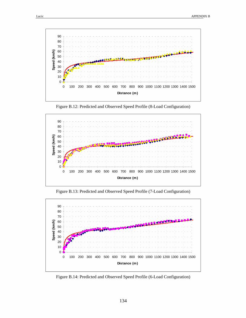
Lucic APPENDIX B
134
0102030405060708090
0 100 200 300 400 500 600 700 800 900 1000 1100 1200 1300 1400 1500
Distance (m)
Spee
d (k
m/h
)
Figure B.12: Predicted and Observed Speed Profile (8-Load Configuration)
0102030405060708090
0 100 200 300 400 500 600 700 800 900 1000 1100 1200 1300 1400 1500
Distance (m)
Spee
d (k
m/h
)
Figure B.13: Predicted and Observed Speed Profile (7-Load Configuration)
0102030405060708090
0 100 200 300 400 500 600 700 800 900 1000 1100 1200 1300 1400 1500
Distance (m)
Spee
d (k
m/h
)
Figure B.14: Predicted and Observed Speed Profile (6-Load Configuration)

Lucic APPENDIX B
135
0102030405060708090
0 100 200 300 400 500 600 700 800 900 1000 1100 1200 1300 1400 1500
Distance (m)
Spee
d (k
m/h
)
Figure B.15: Predicted and Observed Speed Profile (5-Load Configuration)
0102030405060708090
0 100 200 300 400 500 600 700 800 900 1000 1100 1200 1300 1400 1500
Distance (m)
Spee
d (k
m/h
)
Figure B.16: Predicted and Observed Speed Profile (4-Load Configuration)
0102030405060708090
0 100 200 300 400 500 600 700 800 900 1000 1100 1200 1300 1400 1500
Distance (m)
Spee
d (k
m/h
)
Figure B.17: Predicted and Observed Speed Profile (3-Load Configuration)

Lucic APPENDIX B
136
0102030405060708090
100110120130140
0 100 200 300 400 500 600 700 800 900 1000 1100 1200 1300 1400 1500
Distance (m)
Spee
d (k
m/h
)
Figure B.18: Predicted and Observed Speed Profile (2-Load Configuration)
0
20
40
60
80
100
120
140
0 100 200 300 400 500 600 700 800 900 1000 1100 1200 1300 1400 1500
Distance (m)
Spee
d (k
m/h
)
Figure B.19: Predicted and Observed Speed Profile (1-Load Configuration)
0
20
40
60
80
100
120
140
0 100 200 300 400 500 600 700 800 900 1000 1100 1200 1300 1400 1500
Distance (m)
Spee
d (k
m/h
)
Figure B.20: Predicted and Observed Speed Profile (0-Load Configuration)

Lucic APPENDIX B
137
0102030405060708090
100110120130140
0 100 200 300 400 500 600 700 800 900 1000 1100 1200 1300 1400 1500
Distance (m)
Spee
d (k
m/h
)
Figure B.21: Predicted and Observed Speed Profile (Truck Configuration)
350 kW (470 hp) truck
Table B.22: Example Solution to ODE (9-Load Configuration) T S v a F i Ra Rr Rg R
0 0.00 0.00 0.00 94479 0.0596 0.00 2481.73 25876.55 28358.28 1 0.60 4.84 1.49 94479 0.0596 6.52 2567.82 25877.42 28451.75 2 2.69 10.21 1.49 94479 0.0596 29.01 2663.31 25880.31 28572.63 3 6.26 15.21 1.11 78014 0.0596 64.42 2752.33 25884.91 28701.67 4 10.98 18.62 0.79 63718 0.0597 96.57 2813.05 25890.38 28800.00 5 16.52 21.15 0.61 56090 0.0597 124.63 2858.11 25895.87 28878.60 6 22.69 23.17 0.50 51201 0.0597 149.56 2894.04 25900.81 28944.41 7 29.36 24.85 0.42 47750 0.0597 171.96 2923.84 25904.78 29000.59 8 36.47 26.27 0.36 45162 0.0597 192.24 2949.18 25907.46 29048.87 9 43.94 27.50 0.32 43139 0.0597 210.69 2971.10 25908.55 29090.34
10 51.73 28.58 0.28 41509 0.0597 227.55 2990.31 25907.82 29125.69
Table B.23: Example Solution to ODE (8-Load Configuration) T S v a F i Ra Rr Rg R
0 0.00 0.00 0.00 93038 0.0596 0.00 2319.44 24184.34 26503.77 1 0.65 5.21 1.61 93038 0.0596 7.56 2406.06 24185.21 26598.82 2 2.90 10.99 1.60 93038 0.0596 33.62 2502.15 24188.11 26723.88 3 6.72 16.17 1.13 73399 0.0596 72.78 2588.24 24192.68 26853.70 4 11.72 19.64 0.81 60422 0.0597 107.40 2645.98 24198.00 26951.37 5 17.55 22.24 0.64 53339 0.0597 137.81 2689.34 24203.24 27030.40 6 24.03 24.34 0.52 48747 0.0597 165.00 2724.18 24207.86 27097.04 7 31.04 26.09 0.44 45483 0.0597 189.53 2753.24 24211.45 27154.22 8 38.50 27.58 0.38 43021 0.0597 211.84 2778.05 24213.66 27203.55 9 46.34 28.88 0.33 41090 0.0597 232.22 2799.61 24214.22 27246.05
10 54.52 30.02 0.30 39529 0.0597 250.92 2818.57 24212.89 27282.39

Lucic APPENDIX B
138
Table B.24: Example Solution to ODE (7-Load Configuration) T S v a F i Ra Rr Rg R
0 0.00 0.00 0.00 86579 0.0596 0.00 2210.05 23043.82 25253.87 1 0.63 5.04 1.55 86579 0.0596 7.07 2289.89 23044.62 25341.58 2 2.81 10.63 1.55 86579 0.0596 31.46 2378.46 23047.30 25457.22 3 6.52 15.98 1.23 74228 0.0596 71.16 2463.33 23051.56 25586.04 4 11.52 19.76 0.87 60051 0.0597 108.73 2523.12 23056.65 25688.49 5 17.41 22.56 0.68 52597 0.0597 141.73 2567.49 23061.72 25770.94 6 24.00 24.80 0.56 47849 0.0597 171.25 2602.96 23066.22 25840.42 7 31.15 26.66 0.47 44505 0.0597 197.95 2632.47 23069.69 25900.11 8 38.79 28.25 0.41 42001 0.0597 222.25 2657.65 23071.81 25951.72 9 46.83 29.63 0.36 40044 0.0597 244.51 2679.53 23072.27 25996.30
10 55.23 30.84 0.32 38468 0.0597 264.96 2698.77 23070.83 26034.56
Table B.25: Example Solution to ODE (6-Load Configuration) T S v a F i Ra Rr Rg R
0 0.00 0.00 0.00 80334 0.0596 0.00 2091.00 21802.51 23893.51 1 0.61 4.90 1.51 80334 0.0596 6.69 2164.48 21803.24 23974.42 2 2.73 10.34 1.51 80334 0.0596 29.77 2245.99 21805.71 24081.48 3 6.36 15.74 1.37 75373 0.0596 69.02 2326.99 21809.66 24205.66 4 11.34 19.89 0.95 59656 0.0597 110.17 2389.17 21814.48 24313.82 5 17.30 22.92 0.73 51765 0.0597 146.32 2434.61 21819.37 24400.30 6 24.02 25.33 0.60 46842 0.0597 178.69 2470.73 21823.71 24473.13 7 31.34 27.33 0.51 43415 0.0597 208.01 2500.70 21827.06 24535.77 8 39.17 29.03 0.44 40867 0.0597 234.77 2526.25 21829.05 24590.07 9 47.45 30.51 0.38 38885 0.0597 259.31 2548.43 21829.39 24637.13
10 56.11 31.82 0.34 37293 0.0597 281.91 2567.95 21827.82 24677.68
Table B.26: Example Solution to ODE (5-Load Configuration) T S v a F i Ra Rr Rg R
0 0.00 0.00 0.00 76811 0.0596 0.00 1985.18 20699.12 22684.30 1 0.62 4.95 1.53 76811 0.0596 6.83 2055.65 20699.83 22762.30 2 2.76 10.44 1.52 76811 0.0596 30.38 2133.82 20702.19 22866.39 3 6.42 15.92 1.46 74510 0.0596 70.62 2211.82 20705.97 22988.42 4 11.49 20.31 1.00 58432 0.0597 114.84 2274.19 20710.62 23099.64 5 17.59 23.50 0.77 50500 0.0597 153.74 2319.58 20715.33 23188.65 6 24.48 26.03 0.63 45586 0.0597 188.67 2355.62 20719.49 23263.78 7 32.01 28.13 0.53 42180 0.0597 220.38 2385.54 20722.65 23328.56 8 40.08 29.92 0.46 39652 0.0597 249.37 2411.06 20724.44 23384.86 9 48.61 31.48 0.40 37689 0.0597 276.02 2433.24 20724.55 23433.80
10 57.55 32.85 0.36 36114 0.0597 300.62 2452.78 20722.72 23476.12
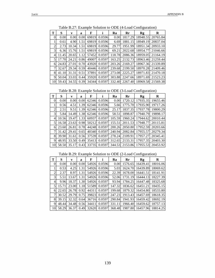
Lucic APPENDIX B
139
Table B.27: Example Solution to ODE (4-Load Configuration) T S v a F i Ra Rr Rg R
0 0.00 0.00 0.00 69819 0.0596 0.00 1817.29 18948.55 20765.84 1 0.61 4.90 1.51 69819 0.0596 6.69 1881.15 18949.19 20837.04 2 2.73 10.34 1.51 69819 0.0596 29.77 1951.99 18951.34 20933.10 3 6.36 15.76 1.51 69819 0.0596 69.21 2022.68 18954.77 21046.66 4 11.45 20.65 1.12 57452 0.0597 118.78 2086.36 18959.05 21164.19 5 17.70 24.21 0.86 49007 0.0597 163.25 2132.73 18963.46 21259.44 6 24.83 27.01 0.70 43920 0.0597 203.26 2169.27 18967.36 21339.89 7 32.67 29.34 0.59 40446 0.0597 239.68 2199.50 18970.28 21409.46 8 41.10 31.31 0.51 37891 0.0597 273.08 2225.27 18971.83 21470.18 9 50.04 33.03 0.44 35920 0.0597 303.88 2247.66 18971.69 21523.23
10 59.43 34.55 0.39 34344 0.0597 332.40 2267.40 18969.58 21569.38
Table B.28: Example Solution to ODE (3-Load Configuration) T S v a F i Ra Rr Rg R
0 0.00 0.00 0.00 62346 0.0596 0.00 1720.12 17935.35 19655.46 1 0.56 4.51 1.39 62346 0.0596 5.66 1775.70 17935.90 19717.26 2 2.51 9.51 1.39 62346 0.0596 25.17 1837.35 17937.78 19800.29 3 5.84 14.49 1.38 62346 0.0596 58.51 1898.87 17940.79 19898.17 4 10.56 19.47 1.33 60937 0.0597 105.59 1960.24 17944.62 20010.44 5 16.58 23.63 0.98 50212 0.0597 155.51 2011.53 17948.77 20115.81 6 23.60 26.81 0.78 44248 0.0597 200.26 2050.80 17952.59 20203.66 7 31.42 29.41 0.65 40340 0.0597 240.94 2082.84 17955.57 20279.34 8 39.90 31.61 0.56 37539 0.0597 278.24 2109.91 17957.27 20345.41 9 48.95 33.50 0.49 35413 0.0597 312.65 2133.31 17957.35 20403.30
10 58.50 35.17 0.43 33735 0.0597 344.53 2153.86 17955.53 20453.92
Table B.29: Example Solution to ODE (2-Load Configuration) T S v a F i Ra Rr Rg R
0 0.00 0.00 0.00 54926 0.0596 0.00 1576.65 16439.41 18016.06 1 0.53 4.25 1.31 54926 0.0596 5.03 1624.70 16439.89 18069.62 2 2.37 8.97 1.31 54926 0.0596 22.39 1678.00 16441.51 18141.91 3 5.51 13.67 1.31 54926 0.0596 52.06 1731.19 16444.13 18227.39 4 9.96 18.37 1.30 54926 0.0597 93.94 1784.25 16447.48 18325.68 5 15.71 23.00 1.18 51589 0.0597 147.32 1836.62 16451.21 18435.15 6 22.65 26.78 0.92 44311 0.0597 199.68 1879.32 16454.80 18533.80 7 30.52 29.79 0.75 39823 0.0597 247.23 1913.43 16457.69 18618.35 8 39.15 32.32 0.64 36716 0.0597 290.84 1941.93 16459.42 18692.19 9 48.44 34.48 0.56 34411 0.0597 331.11 1966.40 16459.62 18757.13
10 58.29 36.37 0.49 32620 0.0597 368.48 1987.80 16457.96 18814.25

Lucic APPENDIX B
140
Table B.30: Example Solution to ODE (1-Load Configuration) T S v a F i Ra Rr Rg R
0 0.00 0.00 0.00 45051 0.0596 0.00 1420.46 14810.85 16231.31 1 0.46 3.68 1.14 45051 0.0596 3.78 1457.98 14811.23 16272.99 2 2.05 7.77 1.13 45051 0.0596 16.82 1499.60 14812.50 16328.92 3 4.78 11.85 1.13 45051 0.0596 39.11 1541.13 14814.57 16394.81 4 8.63 15.92 1.13 45051 0.0597 70.57 1582.56 14817.26 16470.39 5 13.62 19.97 1.13 45051 0.0597 111.12 1623.88 14820.33 16555.33 6 19.73 24.02 1.12 45051 0.0597 160.67 1665.06 14823.47 16649.20 7 26.96 27.98 1.01 42399 0.0597 218.11 1705.45 14826.29 16749.84 8 35.21 31.31 0.83 37891 0.0597 273.08 1739.35 14828.34 16840.77 9 44.30 34.09 0.71 34804 0.0597 323.67 1767.63 14829.17 16920.47
10 54.11 36.47 0.61 32529 0.0597 370.53 1791.91 14828.41 16990.85
Table B.31: Example Solution to ODE (0-Load Configuration) T S v a F i Ra Rr Rg R
0 0.00 0.00 0.00 45638 0.0596 0.00 1258.67 13123.94 14382.61 1 0.56 4.51 1.39 45638 0.0596 5.66 1299.36 13124.35 14429.38 2 2.51 9.51 1.39 45638 0.0596 25.19 1344.50 13125.72 14495.41 3 5.85 14.50 1.38 45638 0.0596 58.56 1389.52 13127.93 14576.01 4 10.57 19.48 1.38 45638 0.0597 105.64 1434.42 13130.73 14670.80 5 16.67 24.44 1.37 45638 0.0597 166.30 1479.18 13133.80 14779.28 6 24.12 29.13 1.15 40733 0.0597 236.31 1521.53 13136.74 14894.58 7 32.76 32.90 0.94 36063 0.0597 301.48 1555.57 13139.01 14996.05 8 42.34 36.03 0.80 32928 0.0597 361.60 1583.83 13140.13 15085.56 9 52.73 38.72 0.69 30647 0.0597 417.45 1608.04 13139.69 15165.18
10 63.82 41.06 0.61 28896 0.0597 469.58 1629.21 13137.35 15236.14
Table B.32: Example Solution to ODE (Truck Configuration) T S v a F i Ra Rr Rg R
0 0.00 0.00 0.00 25408 0.0596 0.00 469.59 4896.28 5365.87 1 0.97 7.75 2.39 25408 0.0596 16.72 495.67 4896.54 5408.94 2 4.31 16.33 2.38 25408 0.0596 74.29 524.57 4897.40 5496.25 3 10.04 24.87 2.36 25408 0.0597 172.25 553.31 4898.70 5624.27 4 18.12 33.34 2.34 25408 0.0597 309.66 581.84 4900.20 5791.70 5 28.56 41.74 2.32 25408 0.0597 485.22 610.11 4901.55 5996.87 6 41.30 49.93 2.09 23765 0.0597 694.24 637.67 4902.30 6234.21 7 56.16 56.82 1.72 20883 0.0597 899.02 660.86 4901.96 6461.85 8 72.76 62.58 1.47 18960 0.0597 1090.66 680.26 4900.06 6670.98 9 90.85 67.54 1.28 17567 0.0596 1270.47 696.97 4896.20 6863.64
10 110.23 71.89 1.13 16504 0.0596 1439.47 711.62 4890.03 7041.12

Lucic APPENDIX B
141
0102030405060708090
0 100 200 300 400 500 600 700 800 900 1000 1100 1200 1300 1400 1500
Distance (m)
Spee
d (k
m/h
)
Figure B.22: Predicted and Observed Speed Profile (9-Load Configuration)
0102030405060708090
0 100 200 300 400 500 600 700 800 900 1000 1100 1200 1300 1400 1500
Distance (m)
Spee
d (k
m/h
)
Figure B.23: Predicted and Observed Speed Profile (8-Load Configuration)
0
10
20
30
40
50
60
70
80
90
0 100 200 300 400 500 600 700 800 900 1000 1100 1200 1300 1400 1500
Distance (m )
Speed (km/h)
Figure B.24: Predicted and Observed Speed Profile (7-Load Configuration)

Lucic APPENDIX B
142
0102030405060708090
0 100 200 300 400 500 600 700 800 900 1000 1100 1200 1300 1400 1500
Distance (m)
Spee
d (k
m/h
)
Figure B.25: Predicted and Observed Speed Profile (6-Load Configuration)
0102030405060708090
0 100 200 300 400 500 600 700 800 900 1000 1100 1200 1300 1400 1500
Distance (m)
Spee
d (k
m/h
)
Figure B.26: Predicted and Observed Speed Profile (5-Load Configuration)
0102030405060708090
0 100 200 300 400 500 600 700 800 900 1000 1100 1200 1300 1400 1500
Distance (m)
Spee
d (k
m/h
)
Figure B.27: Predicted and Observed Speed Profile (4-Load Configuration)

Lucic APPENDIX B
143
0102030405060708090
0 100 200 300 400 500 600 700 800 900 1000 1100 1200 1300 1400 1500
Distance (m)
Spee
d (k
m/h
)
Figure B.28: Predicted and Observed Speed Profile (3-Load Configuration)
0102030405060708090
0 100 200 300 400 500 600 700 800 900 1000 1100 1200 1300 1400 1500
Distance (m)
Spee
d (k
m/h
)
Figure B.29: Predicted and Observed Speed Profile (2-Load Configuration)
0102030405060708090
0 100 200 300 400 500 600 700 800 900 1000 1100 1200 1300 1400 1500
Distance (m)
Spee
d (k
m/h
)
Figure B.30: Predicted and Observed Speed Profile (1-Load Configuration)

Lucic APPENDIX B
144
0
20
40
60
80
100
120
140
0 100 200 300 400 500 600 700 800 900 1000 1100 1200 1300 1400 1500
Distance (m)
Spee
d (k
m/h
)
Figure B.31: Predicted and Observed Speed Profile (0-Load Configuration)
0
20
40
60
80
100
120
140
0 100 200 300 400 500 600 700 800 900 1000 1100 1200 1300 1400 1500
Distance (m )
Speed (km/h)
Figure B.32: Predicted and Observed Speed Profile (Truck Configuration)

Lucic APPENDIX B
145
375 kW (500 hp) truck
Table B.33: Example Solution to ODE (9-Load Configuration) T S v a F i Ra Rr Rg R
0 0.00 0.00 0.00 99858 0.0596 0.00 2512.77 26200.14 28712.91 1 0.64 5.14 1.59 99858 0.0596 8.12 2605.39 26201.07 28814.59 2 2.86 10.85 1.58 99858 0.0596 36.15 2708.14 26204.18 28948.46 3 6.63 15.97 1.11 79042 0.0596 78.37 2800.45 26209.07 29087.90 4 11.57 19.41 0.80 65045 0.0597 115.73 2862.36 26214.78 29192.87 5 17.33 21.98 0.63 57420 0.0597 148.50 2908.78 26220.43 29277.71 6 23.74 24.05 0.52 52484 0.0597 177.76 2946.03 26225.43 29349.21 7 30.66 25.77 0.44 48976 0.0597 204.13 2977.06 26229.34 29410.53 8 38.03 27.24 0.38 46333 0.0597 228.08 3003.54 26231.81 29463.43 9 45.78 28.52 0.33 44261 0.0597 249.94 3026.52 26232.54 29509.00
10 53.86 29.64 0.29 42586 0.0597 269.98 3046.72 26231.27 29547.97
Table B.34: Example Solution to ODE (8-Load Configuration) T S v a F i Ra Rr Rg R
0 0.00 0.00 0.00 97071 0.0596 0.00 2374.76 24761.23 27135.99 1 0.67 5.35 1.65 97071 0.0596 8.79 2465.81 24762.14 27236.74 2 2.98 11.28 1.65 97071 0.0596 39.10 2566.81 24765.19 27371.10 3 6.89 16.57 1.15 76176 0.0596 84.38 2656.88 24769.98 27511.24 4 12.02 20.12 0.83 62732 0.0597 124.42 2717.34 24775.52 27617.28 5 17.99 22.80 0.65 55371 0.0597 159.70 2762.88 24780.95 27703.53 6 24.63 24.95 0.54 50591 0.0597 191.31 2799.55 24785.69 27776.55 7 31.82 26.75 0.46 47187 0.0597 219.90 2830.19 24789.30 27839.39 8 39.47 28.29 0.39 44619 0.0597 245.94 2856.41 24791.42 27893.78 9 47.52 29.63 0.35 42601 0.0597 269.79 2879.22 24791.75 27940.76
10 55.91 30.81 0.31 40969 0.0597 291.71 2899.31 24790.04 27981.06
Table B.35: Example Solution to ODE (7-Load Configuration) T S v a F i Ra Rr Rg R
0 0.00 0.00 0.00 94131 0.0596 0.00 2236.76 23322.32 25559.08 1 0.70 5.57 1.72 94131 0.0596 9.52 2326.04 23323.21 25658.77 2 3.10 11.74 1.71 94131 0.0596 42.37 2425.06 23326.20 25793.63 3 7.17 17.21 1.19 73333 0.0597 91.05 2512.79 23330.86 25934.69 4 12.49 20.89 0.86 60414 0.0597 134.15 2571.81 23336.22 26042.18 5 18.70 23.68 0.68 53310 0.0597 172.29 2616.46 23341.42 26130.17 6 25.60 25.93 0.56 48684 0.0597 206.58 2652.53 23345.90 26205.01 7 33.07 27.81 0.48 45385 0.0597 237.71 2682.76 23349.20 26269.67 8 41.02 29.43 0.42 42891 0.0597 266.15 2708.69 23350.96 26325.80 9 49.40 30.84 0.36 40930 0.0597 292.27 2731.30 23350.88 26374.45
10 58.14 32.08 0.32 39341 0.0597 316.35 2751.27 23348.70 26416.32
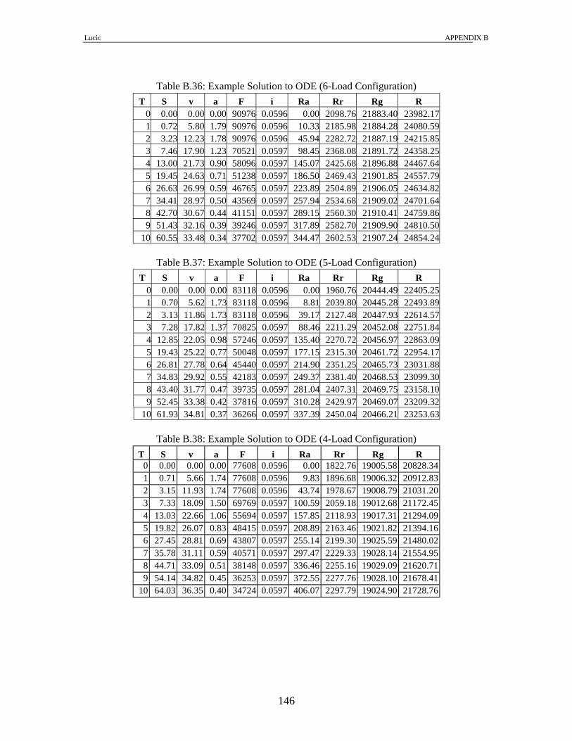
Lucic APPENDIX B
146
Table B.36: Example Solution to ODE (6-Load Configuration)
T S v a F i Ra Rr Rg R 0 0.00 0.00 0.00 90976 0.0596 0.00 2098.76 21883.40 23982.17 1 0.72 5.80 1.79 90976 0.0596 10.33 2185.98 21884.28 24080.59 2 3.23 12.23 1.78 90976 0.0596 45.94 2282.72 21887.19 24215.85 3 7.46 17.90 1.23 70521 0.0597 98.45 2368.08 21891.72 24358.25 4 13.00 21.73 0.90 58096 0.0597 145.07 2425.68 21896.88 24467.64 5 19.45 24.63 0.71 51238 0.0597 186.50 2469.43 21901.85 24557.79 6 26.63 26.99 0.59 46765 0.0597 223.89 2504.89 21906.05 24634.82 7 34.41 28.97 0.50 43569 0.0597 257.94 2534.68 21909.02 24701.64 8 42.70 30.67 0.44 41151 0.0597 289.15 2560.30 21910.41 24759.86 9 51.43 32.16 0.39 39246 0.0597 317.89 2582.70 21909.90 24810.50
10 60.55 33.48 0.34 37702 0.0597 344.47 2602.53 21907.24 24854.24
Table B.37: Example Solution to ODE (5-Load Configuration) T S v a F i Ra Rr Rg R
0 0.00 0.00 0.00 83118 0.0596 0.00 1960.76 20444.49 22405.25 1 0.70 5.62 1.73 83118 0.0596 8.81 2039.80 20445.28 22493.89 2 3.13 11.86 1.73 83118 0.0596 39.17 2127.48 20447.93 22614.57 3 7.28 17.82 1.37 70825 0.0597 88.46 2211.29 20452.08 22751.84 4 12.85 22.05 0.98 57246 0.0597 135.40 2270.72 20456.97 22863.09 5 19.43 25.22 0.77 50048 0.0597 177.15 2315.30 20461.72 22954.17 6 26.81 27.78 0.64 45440 0.0597 214.90 2351.25 20465.73 23031.88 7 34.83 29.92 0.55 42183 0.0597 249.37 2381.40 20468.53 23099.30 8 43.40 31.77 0.47 39735 0.0597 281.04 2407.31 20469.75 23158.10 9 52.45 33.38 0.42 37816 0.0597 310.28 2429.97 20469.07 23209.32
10 61.93 34.81 0.37 36266 0.0597 337.39 2450.04 20466.21 23253.63
Table B.38: Example Solution to ODE (4-Load Configuration) T S v a F i Ra Rr Rg R
0 0.00 0.00 0.00 77608 0.0596 0.00 1822.76 19005.58 20828.34 1 0.71 5.66 1.74 77608 0.0596 9.83 1896.68 19006.32 20912.83 2 3.15 11.93 1.74 77608 0.0596 43.74 1978.67 19008.79 21031.20 3 7.33 18.09 1.50 69769 0.0597 100.59 2059.18 19012.68 21172.45 4 13.03 22.66 1.06 55694 0.0597 157.85 2118.93 19017.31 21294.09 5 19.82 26.07 0.83 48415 0.0597 208.89 2163.46 19021.82 21394.16 6 27.45 28.81 0.69 43807 0.0597 255.14 2199.30 19025.59 21480.02 7 35.78 31.11 0.59 40571 0.0597 297.47 2229.33 19028.14 21554.95 8 44.71 33.09 0.51 38148 0.0597 336.46 2255.16 19029.09 21620.71 9 54.14 34.82 0.45 36253 0.0597 372.55 2277.76 19028.10 21678.41
10 64.03 36.35 0.40 34724 0.0597 406.07 2297.79 19024.90 21728.76

Lucic APPENDIX B
147
Table B.39: Example Solution to ODE (3-Load Configuration) T S v a F i Ra Rr Rg R
0 0.00 0.00 0.00 72483 0.0596 0.00 1684.76 17566.67 19251.43 1 0.72 5.74 1.77 72483 0.0596 10.12 1754.06 17567.36 19331.54 2 3.20 12.10 1.77 72483 0.0596 45.00 1830.92 17569.67 19445.60 3 7.44 18.43 1.63 68489 0.0597 104.38 1907.37 17573.32 19585.07 4 13.29 23.38 1.14 53985 0.0597 168.01 1967.17 17577.69 19712.87 5 20.31 27.05 0.89 46665 0.0597 224.85 2011.47 17581.94 19818.26 6 28.25 30.00 0.74 42081 0.0597 276.51 2047.07 17585.45 19909.02 7 36.93 32.47 0.63 38879 0.0597 323.92 2076.90 17587.73 19988.54 8 46.25 34.59 0.55 36491 0.0597 367.70 2102.56 17588.38 20058.64 9 56.12 36.45 0.48 34628 0.0597 408.34 2125.04 17587.06 20120.44
10 66.48 38.10 0.43 33127 0.0597 446.18 2144.99 17583.48 20174.65
Table B.40: Example Solution to ODE (2-Load Configuration) T S v a F i Ra Rr Rg R
0 0.00 0.00 0.00 65962 0.0596 0.00 1546.76 16127.75 17674.51 1 0.71 5.67 1.75 65962 0.0596 9.88 1609.62 16128.38 17747.88 2 3.16 11.96 1.74 65962 0.0596 43.93 1679.34 16130.48 17853.76 3 7.35 18.23 1.74 65962 0.0597 102.11 1748.90 16133.80 17984.80 4 13.22 23.76 1.27 53128 0.0597 173.47 1810.22 16137.83 18121.52 5 20.41 27.82 0.98 45375 0.0597 237.81 1855.24 16141.83 18234.87 6 28.60 31.06 0.81 40645 0.0597 296.39 1891.14 16145.11 18332.64 7 37.62 33.76 0.69 37389 0.0597 350.25 1921.13 16147.19 18418.57 8 47.32 36.08 0.60 34982 0.0597 400.12 1946.89 16147.65 18494.65 9 57.63 38.12 0.53 33115 0.0597 446.49 1969.44 16146.12 18562.05
10 68.48 39.92 0.47 31618 0.0597 489.77 1989.45 16142.32 18621.55
Table B.41: Example Solution to ODE (1-Load Configuration) T S v a F i Ra Rr Rg R 0 0.00 0.00 0.00 56353 0.0596 0.00 1408.76 14688.84 16097.60 1 0.65 5.19 1.60 56353 0.0596 8.27 1461.16 14689.37 16158.81 2 2.89 10.94 1.60 56353 0.0596 36.81 1519.29 14691.12 16247.22 3 6.73 16.68 1.59 56353 0.0596 85.55 1577.27 14693.92 16356.74 4 12.16 22.41 1.59 56328 0.0597 154.32 1635.08 14697.40 16486.80 5 19.11 27.37 1.17 46123 0.0597 230.16 1685.16 14701.07 16616.39 6 27.26 31.19 0.95 40468 0.0597 298.99 1723.79 14704.24 16727.02 7 36.37 34.33 0.79 36765 0.0597 362.24 1755.51 14706.37 16824.12 8 46.29 37.00 0.68 34111 0.0597 420.81 1782.49 14706.99 16910.30 9 56.90 39.33 0.60 32095 0.0597 475.33 1805.97 14705.73 16987.03
10 68.11 41.38 0.54 30502 0.0597 526.27 1826.71 14702.26 17055.24

Lucic APPENDIX B
148
Table B.42: Example Solution to ODE (0-Load Configuration) T S v a F i Ra Rr Rg R 0 0.00 0.00 0.00 47754 0.0596 0.00 1270.88 13251.26 14522.14 1 0.59 4.75 1.46 47754 0.0596 6.93 1314.15 13251.69 14572.77 2 2.64 10.01 1.46 47754 0.0596 30.82 1362.13 13253.15 14646.10 3 6.16 15.27 1.46 47754 0.0596 71.64 1409.99 13255.47 14737.10 4 11.12 20.51 1.45 47754 0.0597 129.22 1457.71 13258.42 14845.35 5 17.55 25.72 1.45 47754 0.0597 203.37 1505.27 13261.61 14970.25 6 25.38 30.50 1.16 41387 0.0597 285.85 1548.77 13264.59 15099.21 7 34.40 34.31 0.95 36788 0.0597 361.80 1583.51 13266.77 15212.07 8 44.38 37.49 0.81 33665 0.0597 432.04 1612.51 13267.65 15312.19 9 55.19 40.23 0.70 31375 0.0597 497.41 1637.45 13266.80 15401.66
10 66.70 42.63 0.62 29608 0.0597 558.52 1659.31 13263.86 15481.70
0102030405060708090
0 100 200 300 400 500 600 700 800 900 1000 1100 1200 1300 1400 1500
Distance (m)
Spee
d (k
m/h
)
Figure B.33: Predicted and Observed Speed Profile (9-Load Configuration)
0102030405060708090
0 100 200 300 400 500 600 700 800 900 1000 1100 1200 1300 1400 1500
Distance (m)
Spee
d (k
m/h
)
Figure B.34: Predicted and Observed Speed Profile (8-Load Configuration)

Lucic APPENDIX B
149
0102030405060708090
0 100 200 300 400 500 600 700 800 900 1000 1100 1200 1300 1400 1500
Distance (m)
Spee
d (k
m/h
)
Figure B.35: Predicted and Observed Speed Profile (7-Load Configuration)
0102030405060708090
0 100 200 300 400 500 600 700 800 900 1000 1100 1200 1300 1400 1500
Distance (m)
Spee
d (k
m/h
)
Figure B.36: Predicted and Observed Speed Profile (6-Load Configuration)
0102030405060708090
0 100 200 300 400 500 600 700 800 900 1000 1100 1200 1300 1400 1500
Distance (m)
Spee
d (k
m/h
)
Figure B.37: Predicted and Observed Speed Profile (5-Load Configuration)
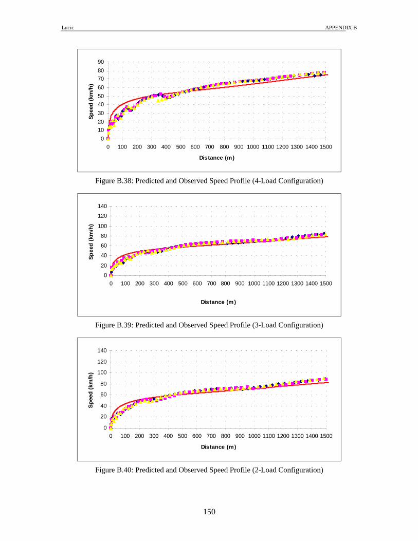
Lucic APPENDIX B
150
0102030405060708090
0 100 200 300 400 500 600 700 800 900 1000 1100 1200 1300 1400 1500
Distance (m)
Spee
d (k
m/h
)
Figure B.38: Predicted and Observed Speed Profile (4-Load Configuration)
0
20
40
60
80
100
120
140
0 100 200 300 400 500 600 700 800 900 1000 1100 1200 1300 1400 1500
Distance (m)
Spee
d (k
m/h
)
Figure B.39: Predicted and Observed Speed Profile (3-Load Configuration)
0
20
40
60
80
100
120
140
0 100 200 300 400 500 600 700 800 900 1000 1100 1200 1300 1400 1500
Distance (m)
Spee
d (k
m/h
)
Figure B.40: Predicted and Observed Speed Profile (2-Load Configuration)

Lucic APPENDIX B
151
0
20
40
60
80
100
120
140
0 100 200 300 400 500 600 700 800 900 1000 1100 1200 1300 1400 1500
Distance (m)
Spee
d (k
m/h
)
Figure B.41: Predicted and Observed Speed Profile (1-Load Configuration)
0102030405060708090
100110120130140
0 100 200 300 400 500 600 700 800 900 1000 1100 1200 1300 1400 1500
Distance (m)
Spee
d (k
m/h
)
Figure B.42: Predicted and Observed Speed Profile (0-Load Configuration)

Lucic APPENDIX B
152
Variable Power Vehicle Dynamics Model 260 kW (350 hp) truck
Table B.43: Example Solution to ODE (9-Load Configuration) T S v a F i Ra Rr Rg R
0 0.00 0.00 0.00 39165 0.0596 0.0 2512.8 26200.1 28712.9 1 0.00 0.00 0.23 39165 0.0596 0.0 2512.8 26200.1 28712.9 2 0.00 0.84 0.23 39165 0.0596 0.3 2527.9 26200.1 28728.3 3 0.23 1.68 0.23 39165 0.0596 1.1 2543.0 26200.5 28744.5 4 0.70 2.52 0.23 39165 0.0596 2.4 2558.1 26201.2 28761.6 5 1.40 3.35 0.23 39165 0.0596 4.2 2573.1 26202.1 28779.5 6 2.33 4.19 0.23 39165 0.0596 6.6 2588.2 26203.4 28798.2 7 3.49 5.02 0.23 39165 0.0596 9.4 2603.2 26205.0 28817.6 8 4.89 5.85 0.23 39165 0.0596 12.8 2618.2 26206.9 28837.8 9 6.51 6.68 0.23 39165 0.0596 16.7 2633.1 26208.9 28858.7
10 8.37 7.51 0.23 39165 0.0597 21.1 2648.0 26211.2 28880.3
Table B.44: Example Solution to ODE (8-Load Configuration) T S v a F i Ra Rr Rg R
0 0.00 0.00 0.00 37598 0.0596 0.0 2374.8 24761.2 27136.0 1 0.00 0.00 0.25 37598 0.0596 0.0 2374.8 24761.2 27136.0 2 0.00 0.89 0.25 37598 0.0596 0.3 2389.9 24761.2 27151.4 3 0.25 1.78 0.25 37598 0.0596 1.2 2405.0 24761.6 27167.8 4 0.74 2.66 0.25 37598 0.0596 2.7 2420.1 24762.2 27185.0 5 1.48 3.55 0.25 37598 0.0596 4.7 2435.2 24763.2 27203.2 6 2.47 4.43 0.25 37598 0.0596 7.4 2450.2 24764.5 27222.1 7 3.70 5.32 0.24 37598 0.0596 10.6 2465.3 24766.1 27242.0 8 5.18 6.20 0.24 37598 0.0596 14.4 2480.3 24767.9 27262.6 9 6.90 7.07 0.24 37598 0.0596 18.7 2495.2 24770.0 27283.9
10 8.86 7.95 0.24 37598 0.0597 23.7 2510.1 24772.2 27306.0
Table B.45: Example Solution to ODE (7-Load Configuration) T S v a F i Ra Rr Rg R
0 0.00 0.00 0.00 37598 0.0596 0.0 2236.8 23322.3 25559.1 1 0.00 0.00 0.30 37598 0.0596 0.0 2236.8 23322.3 25559.1 2 0.00 1.09 0.30 37598 0.0596 0.4 2254.2 23322.3 25576.9 3 0.30 2.17 0.30 37598 0.0596 1.8 2271.6 23322.7 25596.1 4 0.91 3.26 0.30 37598 0.0596 4.0 2289.0 23323.5 25616.4 5 1.81 4.34 0.30 37598 0.0596 7.0 2306.3 23324.6 25638.0 6 3.01 5.42 0.30 37598 0.0596 11.0 2323.6 23326.1 25660.7 7 4.52 6.49 0.30 37598 0.0596 15.8 2340.9 23327.9 25684.6 8 6.32 7.57 0.30 37598 0.0596 21.5 2358.1 23329.9 25709.5 9 8.42 8.64 0.30 37598 0.0597 28.0 2375.4 23332.2 25735.5
10 10.83 9.71 0.30 37598 0.0597 35.3 2392.5 23334.6 25762.5

Lucic APPENDIX B
153
Table B.46: Example Solution to ODE (6-Load Configuration)
T S v a F i Ra Rr Rg R 0 0.00 0.00 0.00 34813 0.0596 0.0 2098.8 21883.4 23982.2 1 0.00 0.00 0.29 34813 0.0596 0.0 2098.8 21883.4 23982.2 2 0.00 1.04 0.29 34813 0.0596 0.4 2114.4 21883.4 23998.3 3 0.29 2.08 0.29 34813 0.0596 1.6 2130.1 21883.8 24015.5 4 0.87 3.12 0.29 34813 0.0596 3.6 2145.7 21884.4 24033.8 5 1.73 4.16 0.29 34813 0.0596 6.5 2161.3 21885.5 24053.3 6 2.89 5.19 0.29 34813 0.0596 10.1 2176.9 21886.8 24073.8 7 4.33 6.23 0.29 34813 0.0596 14.5 2192.4 21888.4 24095.4 8 6.06 7.26 0.29 34813 0.0596 19.7 2208.0 21890.3 24118.0 9 8.08 8.29 0.29 34813 0.0597 25.7 2223.4 21892.3 24141.5
10 10.38 9.31 0.28 34813 0.0597 32.5 2238.9 21894.5 24165.9
Table B.47: Example Solution to ODE (5-Load Configuration) T S v a F i Ra Rr Rg R
0 0.00 0.00 0.00 32412 0.0596 0.0 1960.8 20444.5 22405.3 1 0.00 0.00 0.29 32412 0.0596 0.0 1960.8 20444.5 22405.3 2 0.00 1.03 0.29 32412 0.0596 0.4 1975.2 20444.5 22420.1 3 0.29 2.06 0.29 32412 0.0596 1.6 1989.7 20444.8 22436.1 4 0.86 3.09 0.28 32412 0.0596 3.6 2004.1 20445.5 22453.2 5 1.72 4.11 0.28 32412 0.0596 6.3 2018.6 20446.4 22471.3 6 2.86 5.14 0.28 32412 0.0596 9.9 2033.0 20447.6 22490.5 7 4.28 6.16 0.28 32412 0.0596 14.2 2047.3 20449.1 22510.6 8 5.99 7.18 0.28 32412 0.0596 19.3 2061.6 20450.8 22531.8 9 7.99 8.19 0.28 32412 0.0597 25.1 2076.0 20452.7 22553.8
10 10.26 9.21 0.28 32412 0.0597 31.8 2090.2 20454.8 22576.8
Table B.48: Example Solution to ODE (4-Load Configuration) T S v a F i Ra Rr Rg R
0 0.00 0.00 0.00 31332 0.0596 0.0 1822.8 19005.6 20828.3 1 0.00 0.00 0.32 31332 0.0596 0.0 1822.8 19005.6 20828.3 2 0.00 1.16 0.32 31332 0.0596 0.5 1838.0 19005.6 20844.0 3 0.32 2.33 0.32 31332 0.0596 2.0 1853.1 19005.9 20861.1 4 0.97 3.48 0.32 31332 0.0596 4.5 1868.3 19006.6 20879.4 5 1.94 4.64 0.32 31332 0.0596 8.1 1883.4 19007.6 20899.1 6 3.23 5.80 0.32 31332 0.0596 12.6 1898.5 19008.9 20920.0 7 4.84 6.95 0.32 31332 0.0596 18.1 1913.6 19010.4 20942.1 8 6.77 8.10 0.32 31332 0.0596 24.6 1928.6 19012.2 20965.4 9 9.02 9.25 0.32 31332 0.0597 32.1 1943.6 19014.1 20989.8
10 11.59 10.40 0.32 31332 0.0597 40.5 1958.6 19016.2 21015.3

Lucic APPENDIX B
154
Table B.49: Example Solution to ODE (3-Load Configuration) T S v a F i Ra Rr Rg R
0 0.00 0.00 0.00 28484 0.0596 0.0 1684.8 17566.7 19251.4 1 0.00 0.00 0.31 28484 0.0596 0.0 1684.8 17566.7 19251.4 2 0.00 1.11 0.31 28484 0.0596 0.5 1698.1 17566.7 19265.2 3 0.31 2.21 0.31 28484 0.0596 1.8 1711.5 17567.0 19280.3 4 0.92 3.31 0.31 28484 0.0596 4.1 1724.8 17567.6 19296.5 5 1.84 4.41 0.31 28484 0.0596 7.3 1738.1 17568.4 19313.8 6 3.07 5.51 0.30 28484 0.0596 11.4 1751.4 17569.6 19332.3 7 4.60 6.61 0.30 28484 0.0596 16.4 1764.6 17570.9 19351.9 8 6.44 7.70 0.30 28484 0.0596 22.2 1777.8 17572.5 19372.5 9 8.58 8.80 0.30 28484 0.0597 29.0 1791.0 17574.2 19394.2
10 11.02 9.89 0.30 28484 0.0597 36.6 1804.2 17576.1 19416.9
Table B.50: Example Solution to ODE (2-Load Configuration) T S v a F i Ra Rr Rg R
0 0.00 0.00 0.00 26110 0.0596 0.0 1546.8 16127.8 17674.5 1 0.00 0.00 0.31 26110 0.0596 0.0 1546.8 16127.8 17674.5 2 0.00 1.10 0.31 26110 0.0596 0.5 1559.0 16127.8 17687.2 3 0.31 2.20 0.30 26110 0.0596 1.8 1571.2 16128.0 17701.0 4 0.92 3.30 0.30 26110 0.0596 4.1 1583.3 16128.6 17716.0 5 1.83 4.39 0.30 26110 0.0596 7.2 1595.5 16129.4 17732.1 6 3.05 5.49 0.30 26110 0.0596 11.3 1607.6 16130.4 17749.3 7 4.58 6.58 0.30 26110 0.0596 16.2 1619.7 16131.6 17767.6 8 6.41 7.67 0.30 26110 0.0596 22.0 1631.8 16133.1 17786.9 9 8.54 8.75 0.30 26110 0.0597 28.7 1643.8 16134.7 17807.2
10 10.97 9.84 0.30 26110 0.0597 36.2 1655.9 16136.4 17828.5
Table B.51: Example Solution to ODE (1-Load Configuration) T S v a F i Ra Rr Rg R
0 0.00 0.00 0.00 24736 0.0596 0.0 1408.8 14688.8 16097.6 1 0.00 0.00 0.34 24736 0.0596 0.0 1408.8 14688.8 16097.6 2 0.00 1.24 0.34 24736 0.0596 0.6 1421.3 14688.8 16110.7 3 0.34 2.47 0.34 24736 0.0596 2.3 1433.7 14689.1 16125.2 4 1.03 3.71 0.34 24736 0.0596 5.1 1446.2 14689.7 16141.0 5 2.06 4.94 0.34 24736 0.0596 9.1 1458.6 14690.5 16158.3 6 3.43 6.17 0.34 24736 0.0596 14.3 1471.1 14691.5 16176.9 7 5.15 7.40 0.34 24736 0.0596 20.5 1483.5 14692.8 16196.7 8 7.20 8.62 0.34 24736 0.0597 27.8 1495.8 14694.2 16217.9 9 9.60 9.84 0.34 24736 0.0597 36.3 1508.1 14695.8 16240.2
10 12.33 11.06 0.34 24736 0.0597 45.8 1520.4 14697.5 16263.7

Lucic APPENDIX B
155
Table B.52: Example Solution to ODE (0-Load Configuration) T S v a F i Ra Rr Rg R
0 0.00 0.00 0.00 22380 0.0596 0.0 1270.9 13251.3 14522.1 1 0.00 0.00 0.35 22380 0.0596 0.0 1270.9 13251.3 14522.1
2 0.00 1.25 0.35 22380 0.0596 0.6 1282.3 13251.3 14534.1 3 0.35 2.49 0.35 22380 0.0596 2.3 1293.6 13251.5 14547.5 4 1.04 3.74 0.34 22380 0.0596 5.2 1305.0 13252.0 14562.2 5 2.08 4.98 0.34 22380 0.0596 9.3 1316.3 13252.8 14578.3 6 3.46 6.22 0.34 22380 0.0596 14.5 1327.6 13253.7 14595.8 7 5.19 7.46 0.34 22380 0.0596 20.8 1338.8 13254.9 14614.5 8 7.26 8.69 0.34 22380 0.0597 28.3 1350.1 13256.2 14634.5 9 9.68 9.92 0.34 22380 0.0597 36.9 1361.3 13257.6 14655.7
10 12.43 11.15 0.34 22380 0.0597 46.5 1372.5 13259.1 14678.1
0102030405060708090
0 100 200 300 400 500 600 700 800 900 1000 1100 1200 1300 1400 1500
Distance (m)
Spee
d (k
m/h
)
Figure B.43: Predicted and Observed Speed Profile (9-Load Configuration)
0102030405060708090
0 100 200 300 400 500 600 700 800 900 1000 1100 1200 1300 1400 1500
Distance (m)
Spee
d (k
m/h
)
Figure B.44: Predicted and Observed Speed Profile (8-Load Configuration)

Lucic APPENDIX B
156
010
2030
4050
6070
8090
0 100 200 300 400 500 600 700 800 900 1000 1100 1200 1300 1400 1500
Distance (m)
Spee
d (k
m/h
)
Figure B.45: Predicted and Observed Speed Profile (7-Load Configuration)
0102030405060708090
0 100 200 300 400 500 600 700 800 900 1000 1100 1200 1300 1400 1500
Distance (m)
Spee
d (k
m/h
)
Figure B.46: Predicted and Observed Speed Profile (6-Load Configuration)
0102030405060708090
0 100 200 300 400 500 600 700 800 900 1000 1100 1200 1300 1400 1500
Distance (m)
Spee
d (k
m/h
)
Figure B.47: Predicted and Observed Speed Profile (5-Load Configuration)

Lucic APPENDIX B
157
0102030405060708090
0 100 200 300 400 500 600 700 800 900 1000 1100 1200 1300 1400 1500
Distance (m)
Spee
d (k
m/h
)
Figure B.48: Predicted and Observed Speed Profile (4-Load Configuration)
0
10
20
30
4050
60
70
80
90
0 100 200 300 400 500 600 700 800 900 1000 1100 1200 1300 1400 1500Distance (m)
Spee
d (k
m/h
)
Figure B.49: Predicted and Observed Speed Profile (3-Load Configuration)
0102030405060708090
0 100 200 300 400 500 600 700 800 900 1000 1100 1200 1300 1400 1500
Distance (m)
Spee
d (k
m/h
)
Figure B.50: Predicted and Observed Speed Profile (2-Load Configuration)

Lucic APPENDIX B
158
0102030405060708090
0 100 200 300 400 500 600 700 800 900 1000 1100 1200 1300 1400 1500
Distance (m)
Spee
d (k
m/h
)
Figure B.51: Predicted and Observed Speed Profile (1-Load Configuration)
0102030405060708090
0 100 200 300 400 500 600 700 800 900 1000 1100 1200 1300 1400 1500
Distance (m)
Spee
d (k
m/h
)
Figure B.52: Predicted and Observed Speed Profile (0-Load Configuration)

Lucic APPENDIX B
159
320 kW (430 hp) truck
Table B.53: Example Solution to ODE (9-Load Configuration) T S v a F i Ra Rr Rg R
0 0.00 0.00 1.61 96881 0.0596 0.0 2409.0 25118.0 27527.0 1 0.00 5.81 0.22 37252 0.0596 9.4 2509.4 25118.0 27636.7 2 1.61 6.62 0.22 37252 0.0596 12.2 2523.3 25120.2 27655.7 3 3.45 7.42 0.22 37252 0.0596 15.3 2537.2 25122.6 27675.1 4 5.51 8.23 0.22 37252 0.0596 18.8 2551.0 25125.2 27695.1 5 7.80 9.03 0.22 37252 0.0597 22.7 2564.9 25127.9 27715.5 6 10.31 9.83 0.22 37252 0.0597 26.9 2578.7 25130.7 27736.2 7 13.04 10.62 0.22 37252 0.0597 31.4 2592.4 25133.5 27757.4 8 15.99 11.42 0.22 37252 0.0597 36.3 2606.2 25136.3 27778.8 9 19.16 12.21 0.22 37252 0.0597 41.5 2619.9 25138.9 27800.4
10 22.55 13.00 0.22 37252 0.0597 47.1 2633.6 25141.4 27822.1
Table B.54: Example Solution to ODE (8-Load Configuration) T S v a F i Ra Rr Rg R
0 0.00 0.00 0.00 37252 0.0596 0.0 2288.4 23860.7 26149.2 1 0.00 0.00 0.27 37252 0.0596 0.0 2288.4 23860.7 26149.2 2 0.00 0.98 0.27 37252 0.0596 0.3 2304.5 23860.7 26165.5 3 0.27 1.96 0.27 37252 0.0596 1.1 2320.5 23861.1 26182.7 4 0.82 2.93 0.27 37252 0.0596 2.4 2336.5 23861.8 26200.8 5 1.63 3.91 0.27 37252 0.0596 4.3 2352.5 23862.9 26219.7 6 2.72 4.88 0.27 37252 0.0596 6.6 2368.5 23864.2 26239.4 7 4.07 5.85 0.27 37252 0.0596 9.5 2384.4 23865.9 26259.9 8 5.70 6.82 0.27 37252 0.0596 13.0 2400.4 23867.8 26281.1 9 7.59 7.79 0.27 37252 0.0597 16.9 2416.2 23870.0 26303.1
10 9.76 8.76 0.27 37252 0.0597 21.4 2432.1 23872.3 26325.7
Table B.55: Example Solution to ODE (7-Load Configuration) T S v a F i Ra Rr Rg R
0 0.00 0.00 0.00 36088 0.0596 0.0 2175.5 22683.1 24858.6 1 0.00 0.00 0.29 36088 0.0596 0.0 2175.5 22683.1 24858.6 2 0.00 1.04 0.29 36088 0.0596 0.3 2191.7 22683.1 24875.1 3 0.29 2.08 0.29 36088 0.0596 1.2 2207.9 22683.5 24892.6 4 0.87 3.12 0.29 36088 0.0596 2.7 2224.1 22684.2 24911.0 5 1.74 4.16 0.29 36088 0.0596 4.8 2240.3 22685.2 24930.4 6 2.89 5.19 0.29 36088 0.0596 7.5 2256.5 22686.6 24950.6 7 4.33 6.23 0.29 36088 0.0596 10.8 2272.6 22688.3 24971.7 8 6.06 7.26 0.29 36088 0.0596 14.7 2288.7 22690.2 24993.6 9 8.08 8.29 0.29 36088 0.0597 19.1 2304.7 22692.4 25016.2
10 10.38 9.32 0.28 36088 0.0597 24.2 2320.8 22694.6 25039.6

Lucic APPENDIX B
160
Table B.56: Example Solution to ODE (6-Load Configuration) T S v a F i Ra Rr Rg R
0 0.00 0.00 0.00 34994 0.0596 0.0 2027.9 21144.7 23172.6 1 0.00 0.00 0.33 34994 0.0596 0.0 2027.9 21144.7 23172.6 2 0.00 1.18 0.33 34994 0.0596 0.4 2045.0 21144.7 23190.1 3 0.33 2.35 0.33 34994 0.0596 1.5 2062.1 21145.1 23208.8 4 0.98 3.53 0.33 34994 0.0596 3.5 2079.2 21145.9 23228.5 5 1.96 4.70 0.32 34994 0.0596 6.1 2096.2 21147.0 23249.3 6 3.26 5.87 0.32 34994 0.0596 9.6 2113.2 21148.4 23271.2 7 4.89 7.03 0.32 34994 0.0596 13.8 2130.2 21150.2 23294.1 8 6.85 8.20 0.32 34994 0.0596 18.7 2147.1 21152.1 23318.0 9 9.12 9.36 0.32 34994 0.0597 24.4 2164.0 21154.3 23342.7
10 11.72 10.52 0.32 34994 0.0597 30.8 2180.9 21156.7 23368.4
Table B.57: Example Solution to ODE (5-Load Configuration) T S v a F i Ra Rr Rg R
0 0.00 0.00 0.00 32995 0.0596 0.0 1940.4 20232.3 22172.7 1 0.00 0.00 0.31 32995 0.0596 0.0 1940.4 20232.3 22172.7 2 0.00 1.13 0.31 32995 0.0596 0.4 1956.1 20232.3 22188.7 3 0.31 2.25 0.31 32995 0.0596 1.4 1971.7 20232.7 22205.8 4 0.94 3.37 0.31 32995 0.0596 3.2 1987.3 20233.3 22223.8 5 1.87 4.49 0.31 32995 0.0596 5.6 2002.9 20234.4 22242.9 6 3.12 5.61 0.31 32995 0.0596 8.8 2018.5 20235.7 22262.9 7 4.68 6.73 0.31 32995 0.0596 12.6 2034.0 20237.3 22283.9 8 6.55 7.84 0.31 32995 0.0596 17.1 2049.5 20239.1 22305.8 9 8.73 8.96 0.31 32995 0.0597 22.3 2065.0 20241.1 22328.5
10 11.22 10.07 0.31 32995 0.0597 28.2 2080.4 20243.3 22352.0
Table B.58: Example Solution to ODE (4-Load Configuration) T S v a F i Ra Rr Rg R
0 0.00 0.00 0.00 31211 0.0596 0.0 1797.4 18741.7 20539.1 1 0.00 0.00 0.33 31211 0.0596 0.0 1797.4 18741.7 20539.1 2 0.00 1.20 0.33 31211 0.0596 0.4 1812.9 18741.7 20555.0 3 0.33 2.40 0.33 31211 0.0596 1.6 1828.3 18742.0 20571.9 4 1.00 3.59 0.33 31211 0.0596 3.6 1843.7 18742.7 20590.0 5 2.00 4.78 0.33 31211 0.0596 6.4 1859.1 18743.7 20609.2 6 3.32 5.97 0.33 31211 0.0596 9.9 1874.4 18745.0 20629.4 7 4.98 7.16 0.33 31211 0.0596 14.3 1889.8 18746.6 20650.6 8 6.97 8.35 0.33 31211 0.0596 19.4 1905.0 18748.4 20672.8 9 9.29 9.53 0.33 31211 0.0597 25.3 1920.3 18750.3 20695.9
10 11.94 10.71 0.33 31211 0.0597 32.0 1935.5 18752.4 20719.9

Lucic APPENDIX B
161
Table B.59: Example Solution to ODE (3-Load Configuration) T S v a F i Ra Rr Rg R
0 0.00 0.00 0.00 28870 0.0596 0.0 1646.9 17171.5 18818.3 1 0.00 0.00 0.34 28870 0.0596 0.0 1646.9 17171.5 18818.3 2 0.00 1.23 0.34 28870 0.0596 0.4 1661.4 17171.5 18833.3 3 0.34 2.46 0.34 28870 0.0596 1.7 1675.9 17171.8 18849.4 4 1.03 3.69 0.34 28870 0.0596 3.8 1690.4 17172.4 18866.7 5 2.05 4.92 0.34 28870 0.0596 6.7 1704.9 17173.4 18885.0 6 3.42 6.14 0.34 28870 0.0596 10.5 1719.4 17174.6 18904.5 7 5.12 7.36 0.34 28870 0.0596 15.1 1733.8 17176.1 18925.0 8 7.17 8.58 0.34 28870 0.0597 20.5 1748.2 17177.8 18946.5 9 9.55 9.80 0.34 28870 0.0597 26.7 1762.6 17179.6 18968.9
10 12.28 11.01 0.34 28870 0.0597 33.8 1776.9 17181.6 18992.2
Table B.60: Example Solution to ODE (2-Load Configuration) T S v a F i Ra Rr Rg R
0 0.00 0.00 0.00 28166 0.0596 0.0 1542.1 16078.7 17620.7 1 0.00 0.00 0.38 28166 0.0596 0.0 1542.1 16078.7 17620.7 2 0.00 1.38 0.38 28166 0.0596 0.5 1557.3 16078.7 17636.5 3 0.38 2.76 0.38 28166 0.0596 2.1 1572.6 16079.0 17653.7 4 1.15 4.14 0.38 28166 0.0596 4.8 1587.8 16079.7 17672.2 5 2.30 5.51 0.38 28166 0.0596 8.5 1603.0 16080.7 17692.1 6 3.83 6.88 0.38 28166 0.0596 13.2 1618.1 16082.0 17713.3 7 5.74 8.25 0.38 28166 0.0596 19.0 1633.3 16083.5 17735.7 8 8.03 9.61 0.38 28166 0.0597 25.7 1648.4 16085.2 17759.3 9 10.70 10.98 0.38 28166 0.0597 33.6 1663.4 16087.1 17784.1
10 13.75 12.34 0.38 28166 0.0597 42.4 1678.4 16089.1 17809.9
Table B.61: Example Solution to ODE (1-Load Configuration) T S v a F i Ra Rr Rg R
0 0.00 0.00 0.00 26856 0.0596 0.0 1399.1 14588.1 15987.1 1 0.00 0.00 0.44 26856 0.0596 0.0 1399.1 14588.1 15987.1 2 0.00 1.57 0.44 26856 0.0596 0.7 1414.8 14588.1 16003.6 3 0.44 3.13 0.43 26856 0.0596 2.7 1430.5 14588.4 16021.7 4 1.31 4.70 0.43 26856 0.0596 6.1 1446.2 14589.1 16041.5 5 2.61 6.26 0.43 26856 0.0596 10.9 1461.9 14590.1 16062.9 6 4.35 7.82 0.43 26856 0.0596 17.0 1477.5 14591.4 16085.9 7 6.52 9.37 0.43 26856 0.0596 24.5 1493.1 14592.9 16110.5 8 9.12 10.92 0.43 26856 0.0597 33.2 1508.6 14594.7 16136.5 9 12.16 12.47 0.43 26856 0.0597 43.3 1524.1 14596.6 16164.0
10 15.62 14.01 0.43 26856 0.0597 54.7 1539.6 14598.5 16192.8

Lucic APPENDIX B
162
Table B.62: Example Solution to ODE (0-Load Configuration) T S v a F i Ra Rr Rg R
0 0.00 0.00 0.00 22643 0.0596 0.0 1163.5 12132.0 13295.5 1 0.00 0.00 0.45 22643 0.0596 0.0 1163.5 12132.0 13295.5 2 0.00 1.62 0.45 22643 0.0596 0.7 1177.1 12132.0 13309.8 3 0.45 3.24 0.45 22643 0.0596 2.9 1190.6 12132.3 13325.8 4 1.35 4.86 0.45 22643 0.0596 6.6 1204.1 12132.9 13343.5 5 2.70 6.47 0.45 22643 0.0596 11.7 1217.5 12133.7 13362.9 6 4.50 8.08 0.45 22643 0.0596 18.2 1231.0 12134.8 13384.0 7 6.74 9.69 0.45 22643 0.0596 26.1 1244.4 12136.2 13406.7 8 9.43 11.29 0.44 22643 0.0597 35.5 1257.7 12137.6 13430.9 9 12.57 12.89 0.44 22643 0.0597 46.3 1271.1 12139.2 13456.6
10 16.15 14.48 0.44 22643 0.0597 58.4 1284.4 12140.9 13483.6
Table B.63: Example Solution to ODE (Truck Configuration) T S v a F i Ra Rr Rg R
0 0.00 0.00 0.00 11548 0.0596 0.0 477.7 4981.2 5458.9 1 0.00 0.00 0.71 11548 0.0596 0.0 477.7 4981.2 5458.9 2 0.00 2.57 0.71 11548 0.0596 1.6 486.5 4981.2 5469.3 3 0.71 5.14 0.71 11548 0.0596 6.3 495.3 4981.4 5483.0 4 2.14 7.71 0.71 11548 0.0596 14.3 504.1 4981.7 5500.1 5 4.28 10.26 0.71 11548 0.0596 25.3 512.9 4982.3 5520.4 6 7.13 12.81 0.70 11548 0.0597 39.4 521.6 4983.0 5544.0 7 10.69 15.35 0.70 11548 0.0597 56.5 530.3 4983.8 5570.6 8 14.95 17.87 0.70 11548 0.0597 76.7 538.9 4984.6 5600.2 9 19.92 20.39 0.69 11548 0.0597 99.8 547.5 4985.4 5632.8
10 25.58 22.89 0.69 11548 0.0597 125.8 556.1 4986.2 5668.1
0102030405060708090
0 100 200 300 400 500 600 700 800 900 1000 1100 1200 1300 1400 1500
Distance (m)
Spee
d (k
m/h
)
Figure B.53: Predicted and Observed Speed Profile (9-Load Configuration)

Lucic APPENDIX B
163
0102030405060708090
0 100 200 300 400 500 600 700 800 900 1000 1100 1200 1300 1400 1500
Distance (m)
Spee
d (k
m/h
)
Figure B.54: Predicted and Observed Speed Profile (8-Load Configuration)
0102030405060708090
0 100 200 300 400 500 600 700 800 900 1000 1100 1200 1300 1400 1500
Distance (m)
Spee
d (k
m/h
)
Figure B.55: Predicted and Observed Speed Profile (7-Load Configuration)
0102030405060708090
0 100 200 300 400 500 600 700 800 900 1000 1100 1200 1300 1400 1500
Distance (m)
Spee
d (k
m/h
)
Figure B.56: Predicted and Observed Speed Profile (6-Load Configuration)

Lucic APPENDIX B
164
0102030405060708090
0 100 200 300 400 500 600 700 800 900 1000 1100 1200 1300 1400 1500
Distance (m)
Spee
d (k
m/h
)
Figure B.57: Predicted and Observed Speed Profile (5-Load Configuration)
0102030405060708090
0 100 200 300 400 500 600 700 800 900 1000 1100 1200 1300 1400 1500
Distance (m)
Spee
d (k
m/h
)
Figure B.58: Predicted and Observed Speed Profile (4-Load Configuration)
0102030405060708090
0 100 200 300 400 500 600 700 800 900 1000 1100 1200 1300 1400 1500
Distance (m)
Spee
d (k
m/h
)
Figure B.59: Predicted and Observed Speed Profile (3-Load Configuration)

Lucic APPENDIX B
165
0102030405060708090
100110120130140
0 100 200 300 400 500 600 700 800 900 1000 1100 1200 1300 1400 1500
Distance (m)
Spee
d (k
m/h
)
Figure B.60: Predicted and Observed Speed Profile (2-Load Configuration)
0
20
40
60
80
100
120
140
0 100 200 300 400 500 600 700 800 900 1000 1100 1200 1300 1400 1500
Distance (m)
Spee
d (k
m/h
)
Figure B.61: Predicted and Observed Speed Profile (1-Load Configuration)
0
20
40
60
80
100
120
140
0 100 200 300 400 500 600 700 800 900 1000 1100 1200 1300 1400 1500
Distance (m)
Spee
d (k
m/h
)
Figure B.62: Predicted and Observed Speed Profile (0-Load Configuration)

Lucic APPENDIX B
166
0102030405060708090
100110120130140
0 100 200 300 400 500 600 700 800 900 1000 1100 1200 1300 1400 1500
Distance (m)
Spee
d (k
m/h
)
Figure B.63: Predicted and Observed Speed Profile (Truck Configuration)
350 kW (470 hp) truck
Table B.64: Example Solution to ODE (9-Load Configuration) T S v a F i Ra Rr Rg R
0 0.00 0.00 0.00 38249 0.0596 0.0 2481.7 25876.6 28358.3 1 0.00 0.00 0.22 38249 0.0596 0.0 2481.7 25876.6 28358.3 2 0.00 0.80 0.22 38249 0.0596 0.2 2496.0 25876.6 28372.8 3 0.22 1.61 0.22 38249 0.0596 0.7 2510.3 25876.9 28387.9 4 0.67 2.41 0.22 38249 0.0596 1.6 2524.6 25877.5 28403.7 5 1.34 3.21 0.22 38249 0.0596 2.9 2538.9 25878.5 28420.2 6 2.23 4.01 0.22 38249 0.0596 4.5 2553.1 25879.7 28437.3 7 3.35 4.81 0.22 38249 0.0596 6.4 2567.3 25881.2 28454.9 8 4.68 5.61 0.22 38249 0.0596 8.8 2581.5 25882.9 28473.2 9 6.24 6.40 0.22 38249 0.0596 11.4 2595.6 25884.9 28491.9
10 8.02 7.20 0.22 38249 0.0597 14.4 2609.8 25887.0 28511.2
Table B.65: Example Solution to ODE (8-Load Configuration) T S v a F i Ra Rr Rg R
0 0.00 0.00 0.00 37124 0.0596 0.0 2319.4 24184.3 26503.8 1 0.00 0.00 0.26 37124 0.0596 0.0 2319.4 24184.3 26503.8 2 0.00 0.92 0.26 37124 0.0596 0.2 2334.8 24184.3 26519.4 3 0.26 1.85 0.26 37124 0.0596 1.0 2350.2 24184.7 26535.8 4 0.77 2.77 0.26 37124 0.0596 2.1 2365.5 24185.4 26553.0 5 1.54 3.69 0.26 37124 0.0596 3.8 2380.8 24186.4 26571.0 6 2.56 4.61 0.25 37124 0.0596 5.9 2396.1 24187.7 26589.7 7 3.84 5.53 0.25 37124 0.0596 8.5 2411.3 24189.3 26609.1 8 5.38 6.44 0.25 37124 0.0596 11.6 2426.5 24191.1 26629.2 9 7.17 7.35 0.25 37124 0.0597 15.1 2441.7 24193.2 26650.0
10 9.21 8.27 0.25 37124 0.0597 19.0 2456.9 24195.4 26671.3

Lucic APPENDIX B
167
Table B.66: Example Solution to ODE (7-Load Configuration) T S v a F i Ra Rr Rg R
0 0.00 0.00 0.00 36064 0.0596 0.0 2210.1 23043.8 25253.9 1 0.00 0.00 0.27 36064 0.0596 0.0 2210.1 23043.8 25253.9 2 0.00 0.99 0.27 36064 0.0596 0.3 2225.7 23043.8 25269.8 3 0.27 1.97 0.27 36064 0.0596 1.1 2241.3 23044.2 25286.6 4 0.82 2.96 0.27 36064 0.0596 2.4 2256.9 23044.9 25304.2 5 1.64 3.94 0.27 36064 0.0596 4.3 2272.5 23045.9 25322.7 6 2.74 4.92 0.27 36064 0.0596 6.7 2288.0 23047.2 25342.0 7 4.11 5.90 0.27 36064 0.0596 9.7 2303.6 23048.8 25362.1 8 5.75 6.88 0.27 36064 0.0596 13.2 2319.1 23050.7 25382.9 9 7.66 7.86 0.27 36064 0.0597 17.2 2334.5 23052.8 25404.5
10 9.84 8.83 0.27 36064 0.0597 21.7 2349.9 23055.0 25426.7
Table B.67: Example Solution to ODE (6-Load Configuration) T S v a F i Ra Rr Rg R
0 0.00 0.00 0.00 35062 0.0596 0.0 2091.0 21802.5 23893.5 1 0.00 0.00 0.30 35062 0.0596 0.0 2091.0 21802.5 23893.5 2 0.00 1.08 0.30 35062 0.0596 0.3 2107.2 21802.5 23910.0 3 0.30 2.16 0.30 35062 0.0596 1.3 2123.3 21802.9 23927.5 4 0.90 3.23 0.30 35062 0.0596 2.9 2139.4 21803.6 23945.9 5 1.80 4.30 0.30 35062 0.0596 5.2 2155.5 21804.6 23965.3 6 2.99 5.37 0.30 35062 0.0596 8.0 2171.6 21806.0 23985.6 7 4.48 6.44 0.30 35062 0.0596 11.6 2187.6 21807.7 24006.8 8 6.27 7.51 0.30 35062 0.0596 15.7 2203.6 21809.6 24028.9 9 8.36 8.58 0.30 35062 0.0597 20.5 2219.6 21811.7 24051.8
10 10.74 9.64 0.29 35062 0.0597 25.9 2235.5 21813.9 24075.3
Table B.68: Example Solution to ODE (5-Load Configuration) T S v a F i Ra Rr Rg R
0 0.00 0.00 0.00 34114 0.0596 0.0 1985.2 20699.1 22684.3 1 0.00 0.00 0.32 34114 0.0596 0.0 1985.2 20699.1 22684.3 2 0.00 1.16 0.32 34114 0.0596 0.4 2001.7 20699.1 22701.2 3 0.32 2.32 0.32 34114 0.0596 1.5 2018.2 20699.5 22719.2 4 0.97 3.48 0.32 34114 0.0596 3.4 2034.7 20700.2 22738.3 5 1.94 4.64 0.32 34114 0.0596 6.0 2051.2 20701.3 22758.5 6 3.22 5.79 0.32 34114 0.0596 9.3 2067.6 20702.7 22779.7 7 4.83 6.95 0.32 34114 0.0596 13.4 2084.1 20704.4 22801.9 8 6.76 8.10 0.32 34114 0.0596 18.3 2100.4 20706.3 22825.0 9 9.01 9.25 0.32 34114 0.0597 23.8 2116.8 20708.4 22849.0
10 11.58 10.39 0.32 34114 0.0597 30.1 2133.1 20710.7 22873.8

Lucic APPENDIX B
168
Table B.69: Example Solution to ODE (4-Load Configuration) T S v a F i Ra Rr Rg R
0 0.00 0.00 0.00 31556 0.0596 0.0 1817.3 18948.6 20765.8 1 0.00 0.00 0.33 31556 0.0596 0.0 1817.3 18948.6 20765.8 2 0.00 1.20 0.33 31556 0.0596 0.4 1832.9 18948.6 20781.9 3 0.33 2.40 0.33 31556 0.0596 1.6 1848.5 18948.9 20799.0 4 1.00 3.59 0.33 31556 0.0596 3.6 1864.1 18949.6 20817.3 5 2.00 4.78 0.33 31556 0.0596 6.4 1879.6 18950.6 20836.6 6 3.32 5.97 0.33 31556 0.0596 9.9 1895.1 18951.9 20857.0 7 4.98 7.16 0.33 31556 0.0596 14.3 1910.6 18953.5 20878.4 8 6.97 8.35 0.33 31556 0.0596 19.4 1926.1 18955.3 20900.8 9 9.29 9.53 0.33 31556 0.0597 25.3 1941.5 18957.3 20924.1
10 11.94 10.71 0.33 31556 0.0597 32.0 1956.9 18959.4 20948.3
Table B.70: Example Solution to ODE (3-Load Configuration) T S v a F i Ra Rr Rg R
0 0.00 0.00 0.00 30053 0.0596 0.0 1720.1 17935.3 19655.5 1 0.00 0.00 0.34 30053 0.0596 0.0 1720.1 17935.3 19655.5 2 0.00 1.22 0.34 30053 0.0596 0.4 1735.2 17935.3 19670.9 3 0.34 2.44 0.34 30053 0.0596 1.7 1750.2 17935.7 19687.5 4 1.02 3.66 0.34 30053 0.0596 3.7 1765.2 17936.3 19705.3 5 2.03 4.87 0.34 30053 0.0596 6.6 1780.2 17937.3 19724.1 6 3.38 6.08 0.34 30053 0.0596 10.3 1795.1 17938.6 19744.0 7 5.07 7.29 0.34 30053 0.0596 14.8 1810.1 17940.1 19765.0 8 7.10 8.50 0.33 30053 0.0596 20.1 1824.9 17941.9 19786.9 9 9.46 9.70 0.33 30053 0.0597 26.2 1839.8 17943.8 19809.8
10 12.16 10.91 0.33 30053 0.0597 33.1 1854.6 17945.8 19833.6
Table B.71: Example Solution to ODE (2-Load Configuration) T S v a F i Ra Rr Rg R
0 0.00 0.00 0.00 28687 0.0596 0.0 1576.6 16439.4 18016.1 1 0.00 0.00 0.38 28687 0.0596 0.0 1576.6 16439.4 18016.1 2 0.00 1.37 0.38 28687 0.0596 0.5 1592.1 16439.4 18032.0 3 0.38 2.73 0.38 28687 0.0596 2.1 1607.5 16439.8 18049.3 4 1.14 4.09 0.38 28687 0.0596 4.7 1622.9 16440.4 18068.0 5 2.28 5.45 0.38 28687 0.0596 8.3 1638.3 16441.4 18088.0 6 3.79 6.81 0.38 28687 0.0596 12.9 1653.6 16442.7 18109.3 7 5.68 8.16 0.38 28687 0.0596 18.6 1668.9 16444.3 18131.8 8 7.95 9.52 0.37 28687 0.0597 25.2 1684.2 16446.0 18155.5 9 10.59 10.86 0.37 28687 0.0597 32.9 1699.5 16447.9 18180.3
10 13.61 12.21 0.37 28687 0.0597 41.5 1714.7 16449.9 18206.1

Lucic APPENDIX B
169
Table B.72: Example Solution to ODE (1-Load Configuration) T S v a F i Ra Rr Rg R
0 0.00 0.00 0.00 26297 0.0596 0.0 1420.5 14810.9 16231.3 1 0.00 0.00 0.40 26297 0.0596 0.0 1420.5 14810.9 16231.3 2 0.00 1.43 0.40 26297 0.0596 0.6 1435.0 14810.9 16246.4 3 0.40 2.86 0.40 26297 0.0596 2.3 1449.6 14811.2 16263.0 4 1.19 4.29 0.40 26297 0.0596 5.1 1464.1 14811.8 16281.0 5 2.38 5.71 0.39 26297 0.0596 9.1 1478.6 14812.8 16300.4 6 3.97 7.13 0.39 26297 0.0596 14.2 1493.1 14814.0 16321.2 7 5.95 8.55 0.39 26297 0.0596 20.3 1507.5 14815.4 16343.3 8 8.32 9.96 0.39 26297 0.0597 27.6 1521.9 14817.1 16366.6 9 11.09 11.37 0.39 26297 0.0597 36.0 1536.3 14818.8 16391.1
10 14.25 12.78 0.39 26297 0.0597 45.5 1550.6 14820.7 16416.8
Table B.73: Example Solution to ODE (0-Load Configuration) T S v a F i Ra Rr Rg R
0 0.00 0.00 0.00 25760 0.0596 0.0 1258.7 13123.9 14382.6 1 0.00 0.00 0.51 25760 0.0596 0.0 1258.7 13123.9 14382.6 2 0.00 1.82 0.51 25760 0.0596 0.9 1275.1 13123.9 14400.0 3 0.51 3.65 0.51 25760 0.0596 3.7 1291.6 13124.3 14419.6 4 1.52 5.47 0.50 25760 0.0596 8.3 1308.0 13125.0 14441.4 5 3.04 7.28 0.50 25760 0.0596 14.8 1324.4 13126.1 14465.2 6 5.06 9.09 0.50 25760 0.0596 23.0 1340.7 13127.4 14491.2 7 7.59 10.90 0.50 25760 0.0597 33.1 1357.0 13129.0 14519.1 8 10.61 12.70 0.50 25760 0.0597 44.9 1373.3 13130.8 14549.0 9 14.14 14.50 0.50 25760 0.0597 58.6 1389.5 13132.6 14580.7
10 18.17 16.30 0.50 25760 0.0597 74.0 1405.7 13134.5 14614.1
Table B.74: Example Solution to ODE (Truck Configuration) T S v a F i Ra Rr Rg R
0 0.00 0.00 0.00 11475 0.0596 0.0 469.6 4896.3 5365.9 1 0.00 0.00 0.73 11475 0.0596 0.0 469.6 4896.3 5365.9 2 0.00 2.63 0.73 11475 0.0596 1.9 478.4 4896.3 5376.6 3 0.73 5.25 0.73 11475 0.0596 7.7 487.3 4896.5 5391.4 4 2.19 7.86 0.72 11475 0.0596 17.2 496.1 4896.9 5410.1 5 4.37 10.47 0.72 11475 0.0596 30.5 504.8 4897.4 5432.8 6 7.28 13.07 0.72 11475 0.0597 47.6 513.6 4898.1 5459.3 7 10.91 15.66 0.71 11475 0.0597 68.3 522.3 4898.9 5489.4 8 15.26 18.23 0.71 11475 0.0597 92.5 531.0 4899.7 5523.2 9 20.32 20.79 0.71 11475 0.0597 120.4 539.6 4900.5 5560.5
10 26.10 23.33 0.70 11475 0.0597 151.6 548.1 4901.3 5601.0

Lucic APPENDIX B
170
0102030405060708090
0 100 200 300 400 500 600 700 800 900 1000 1100 1200 1300 1400 1500
Distance (m)
Spee
d (k
m/h
)
Figure B.64: Predicted and Observed Speed Profile (9-Load Configuration)
0102030405060708090
0 100 200 300 400 500 600 700 800 900 1000 1100 1200 1300 1400 1500
Distance (m)
Spee
d (k
m/h
)
Figure B.65: Predicted and Observed Speed Profile (8-Load Configuration)
0.0010.0020.0030.0040.0050.0060.0070.0080.0090.00
0 100 200 300 400 500 600 700 800 900 1000
1100
1200
1300
1400
1500
Distance (m)
Spee
d (k
m/h
)
Figure B.66: Predicted and Observed Speed Profile (7-Load Configuration)

Lucic APPENDIX B
171
0102030405060708090
0 100 200 300 400 500 600 700 800 900 1000 1100 1200 1300 1400 1500
Distance (m)
Spee
d (k
m/h
)
Figure B.67: Predicted and Observed Speed Profile (6-Load Configuration)
0102030405060708090
0 100 200 300 400 500 600 700 800 900 1000 1100 1200 1300 1400 1500
Distance (m)
Spee
d (k
m/h
)
Figure B.68: Predicted and Observed Speed Profile (5-Load Configuration)
0102030405060708090
0 100 200 300 400 500 600 700 800 900 1000 1100 1200 1300 1400 1500
Distance (m)
Spee
d (k
m/h
)
Figure B.69: Predicted and Observed Speed Profile (4-Load Configuration)

Lucic APPENDIX B
172
0102030405060708090
100
0 100 200 300 400 500 600 700 800 900 1000 1100 1200 1300 1400 1500
Distance (m)
Spee
d (k
m/h
)
Figure B.70: Predicted and Observed Speed Profile (3-Load Configuration)
0102030405060708090
100
0 100 200 300 400 500 600 700 800 900 1000 1100 1200 1300 1400 1500
Distance (m)
Spee
d (k
m/h
)
Figure B.71: Predicted and Observed Speed Profile (2-Load Configuration)
0102030405060708090
0 100 200 300 400 500 600 700 800 900 1000 1100 1200 1300 1400 1500
Distance (m)
Spee
d (k
m/h
)
Figure B.72: Predicted and Observed Speed Profile (1-Load Configuration)

Lucic APPENDIX B
173
0
20
40
60
80
100
120
140
0 100 200 300 400 500 600 700 800 900 1000 1100 1200 1300 1400 1500
Distance (m)
Spee
d (k
m/h
)
Figure B.73: Predicted and Observed Speed Profile (0-Load Configuration)
0
20
40
60
80
100
120
140
160
0 100 200 300 400 500 600 700 800 900 1000 1100 1200 1300 1400 1500
Distance (m)
Spee
d (k
m/h
)
Figure B.74: Predicted and Observed Speed Profile (Truck Configuration)

Lucic APPENDIX B
174
375 kW (500 hp) truck
Table B.75: Example Solution to ODE (9-Load Configuration) T S v a F i Ra Rr Rg R
0 0.00 0.00 0.00 41963 0.0596 0.0 2512.8 26200.1 28712.9 1 0.00 0.00 0.30 41963 0.0596 0.0 2512.8 26200.1 28712.9 2 0.00 1.06 0.30 41963 0.0596 0.3 2531.9 26200.1 28732.4 3 0.30 2.13 0.29 41963 0.0596 1.3 2551.1 26200.6 28752.9 4 0.89 3.19 0.29 41963 0.0596 2.8 2570.2 26201.4 28774.5 5 1.77 4.25 0.29 41963 0.0596 5.0 2589.3 26202.7 28797.0 6 2.95 5.31 0.29 41963 0.0596 7.8 2608.4 26204.3 28820.5 7 4.43 6.36 0.29 41963 0.0596 11.3 2627.4 26206.3 28844.9 8 6.19 7.42 0.29 41963 0.0596 15.3 2646.4 26208.5 28870.2 9 8.25 8.47 0.29 41963 0.0597 20.0 2665.3 26211.0 28896.3
10 10.61 9.52 0.29 41963 0.0597 25.2 2684.2 26213.7 28923.2
Table B.76: Example Solution to ODE (8-Load Configuration) T S v a F i Ra Rr Rg R
0 0.00 0.00 0.00 40691 0.0596 0.0 2374.8 24761.2 27136.0 1 0.00 0.00 0.32 40691 0.0596 0.0 2374.8 24761.2 27136.0 2 0.00 1.15 0.32 40691 0.0596 0.4 2394.4 24761.2 27156.0 3 0.32 2.30 0.32 40691 0.0596 1.5 2414.0 24761.7 27177.1 4 0.96 3.45 0.32 40691 0.0596 3.3 2433.5 24762.5 27199.4 5 1.92 4.60 0.32 40691 0.0596 5.9 2453.1 24763.8 27222.8 6 3.20 5.74 0.32 40691 0.0596 9.2 2472.6 24765.5 27247.2 7 4.79 6.89 0.32 40691 0.0596 13.2 2492.0 24767.5 27272.7 8 6.70 8.03 0.32 40691 0.0596 17.9 2511.4 24769.8 27299.1 9 8.93 9.17 0.32 40691 0.0597 23.4 2530.8 24772.3 27326.5
10 11.48 10.30 0.31 40691 0.0597 29.6 2550.2 24775.0 27354.7
Table B.77: Example Solution to ODE (7-Load Configuration) T S v a F i Ra Rr Rg R
0 0.00 0.00 0.00 37300 0.0596 0.0 2236.8 23322.3 25559.1 1 0.00 0.00 0.29 37300 0.0596 0.0 2236.8 23322.3 25559.1 2 0.00 1.06 0.29 37300 0.0596 0.3 2253.8 23322.3 25576.4 3 0.29 2.12 0.29 37300 0.0596 1.2 2270.7 23322.7 25594.7 4 0.88 3.17 0.29 37300 0.0596 2.8 2287.7 23323.4 25613.9 5 1.76 4.23 0.29 37300 0.0596 5.0 2304.6 23324.6 25634.1 6 2.94 5.28 0.29 37300 0.0596 7.8 2321.5 23326.0 25655.2 7 4.41 6.33 0.29 37300 0.0596 11.2 2338.3 23327.7 25677.2 8 6.17 7.38 0.29 37300 0.0596 15.2 2355.2 23329.8 25700.1 9 8.22 8.43 0.29 37300 0.0597 19.8 2371.9 23332.0 25723.7
10 10.56 9.47 0.29 37300 0.0597 25.0 2388.7 23334.4 25748.1

Lucic APPENDIX B
175
Table B.78: Example Solution to ODE (6-Load Configuration)
T S v a F i Ra Rr Rg R 0 0.00 0.00 0.00 36292 0.0596 0.0 2098.8 21883.4 23982.2 1 0.00 0.00 0.33 36292 0.0596 0.0 2098.8 21883.4 23982.2 2 0.00 1.18 0.33 36292 0.0596 0.4 2116.6 21883.4 24000.4 3 0.33 2.37 0.33 36292 0.0596 1.6 2134.4 21883.8 24019.7 4 0.99 3.55 0.33 36292 0.0596 3.5 2152.1 21884.6 24040.2 5 1.97 4.73 0.33 36292 0.0596 6.2 2169.9 21885.7 24061.8 6 3.28 5.90 0.33 36292 0.0596 9.7 2187.6 21887.3 24084.5 7 4.92 7.08 0.33 36292 0.0596 13.9 2205.2 21889.1 24108.2 8 6.89 8.25 0.32 36292 0.0596 18.9 2222.9 21891.1 24133.0 9 9.18 9.42 0.32 36292 0.0597 24.7 2240.5 21893.4 24158.6
10 11.80 10.59 0.32 36292 0.0597 31.2 2258.0 21895.8 24185.1
Table B.79: Example Solution to ODE (5-Load Configuration) T S v a F i Ra Rr Rg R
0 0.00 0.00 0.00 34431 0.0596 0.0 1960.8 20444.5 22405.3 1 0.00 0.00 0.34 34431 0.0596 0.0 1960.8 20444.5 22405.3 2 0.00 1.24 0.34 34431 0.0596 0.4 1978.2 20444.5 22423.1 3 0.34 2.47 0.34 34431 0.0596 1.7 1995.5 20444.9 22442.1 4 1.03 3.71 0.34 34431 0.0596 3.8 2012.9 20445.7 22462.4 5 2.06 4.94 0.34 34431 0.0596 6.8 2030.2 20446.8 22483.8 6 3.43 6.17 0.34 34431 0.0596 10.6 2047.5 20448.2 22506.4 7 5.15 7.40 0.34 34431 0.0596 15.2 2064.8 20450.0 22530.0 8 7.20 8.62 0.34 34431 0.0597 20.7 2082.0 20452.0 22554.7 9 9.60 9.85 0.34 34431 0.0597 27.0 2099.2 20454.2 22580.4
10 12.34 11.07 0.34 34431 0.0597 34.1 2116.3 20456.6 22607.0
Table B.80: Example Solution to ODE (4-Load Configuration) T S v a F i Ra Rr Rg R
0 0.00 0.00 0.00 32751 0.0596 0.0 1822.8 19005.6 20828.3 1 0.00 0.00 0.37 32751 0.0596 0.0 1822.8 19005.6 20828.3 2 0.00 1.32 0.37 32751 0.0596 0.5 1840.0 19005.6 20846.1 3 0.37 2.64 0.37 32751 0.0596 1.9 1857.3 19006.0 20865.2 4 1.10 3.96 0.37 32751 0.0596 4.4 1874.5 19006.7 20885.5 5 2.20 5.27 0.36 32751 0.0596 7.7 1891.6 19007.8 20907.2 6 3.66 6.58 0.36 32751 0.0596 12.1 1908.8 19009.3 20930.1 7 5.49 7.89 0.36 32751 0.0596 17.3 1925.9 19011.0 20954.2 8 7.68 9.20 0.36 32751 0.0597 23.6 1943.0 19013.0 20979.5 9 10.24 10.50 0.36 32751 0.0597 30.7 1960.0 19015.1 21005.9
10 13.16 11.80 0.36 32751 0.0597 38.8 1977.0 19017.4 21033.2

Lucic APPENDIX B
176
Table B.81: Example Solution to ODE (3-Load Configuration) T S v a F i Ra Rr Rg R
0 0.00 0.00 0.00 31971 0.0596 0.0 1684.8 17566.7 19251.4 1 0.00 0.00 0.42 31971 0.0596 0.0 1684.8 17566.7 19251.4 2 0.00 1.52 0.42 31971 0.0596 0.6 1703.2 17566.7 19270.5 3 0.42 3.05 0.42 31971 0.0596 2.6 1721.6 17567.1 19291.2 4 1.27 4.57 0.42 31971 0.0596 5.8 1739.9 17567.9 19313.6 5 2.54 6.08 0.42 31971 0.0596 10.3 1758.2 17569.1 19337.6 6 4.23 7.60 0.42 31971 0.0596 16.1 1776.5 17570.6 19363.2 7 6.34 9.11 0.42 31971 0.0596 23.1 1794.8 17572.4 19390.3 8 8.87 10.62 0.42 31971 0.0597 31.4 1813.0 17574.5 19418.8 9 11.82 12.12 0.42 31971 0.0597 40.9 1831.1 17576.7 19448.7
10 15.18 13.62 0.42 31971 0.0597 51.7 1849.3 17578.9 19479.9
Table B.82: Example Solution to ODE (2-Load Configuration) T S v a F i Ra Rr Rg R
0 0.00 0.00 0.00 29840 0.0596 0.0 1546.8 16127.8 17674.5 1 0.00 0.00 0.44 29840 0.0596 0.0 1546.8 16127.8 17674.5 2 0.00 1.59 0.44 29840 0.0596 0.7 1564.4 16127.8 17692.8 3 0.44 3.17 0.44 29840 0.0596 2.8 1581.9 16128.1 17712.9 4 1.32 4.76 0.44 29840 0.0596 6.3 1599.5 16128.9 17734.7 5 2.64 6.34 0.44 29840 0.0596 11.2 1617.0 16130.1 17758.3 6 4.40 7.91 0.44 29840 0.0596 17.4 1634.5 16131.5 17783.5 7 6.60 9.49 0.44 29840 0.0596 25.1 1652.0 16133.2 17810.3 8 9.24 11.06 0.44 29840 0.0597 34.1 1669.4 16135.2 17838.6 9 12.31 12.62 0.43 29840 0.0597 44.4 1686.7 16137.3 17868.4
10 15.82 14.19 0.43 29840 0.0597 56.1 1704.1 16139.4 17899.5
Table B.83: Example Solution to ODE (1-Load Configuration) T S v a F i Ra Rr Rg R
0 0.00 0.00 0.00 27975 0.0596 0.0 1408.8 14688.8 16097.6 1 0.00 0.00 0.47 27975 0.0596 0.0 1408.8 14688.8 16097.6 2 0.00 1.70 0.47 27975 0.0596 0.8 1425.9 14688.8 16115.6 3 0.47 3.40 0.47 27975 0.0596 3.2 1443.1 14689.2 16135.6 4 1.42 5.10 0.47 27975 0.0596 7.2 1460.3 14690.0 16157.5 5 2.83 6.79 0.47 27975 0.0596 12.8 1477.4 14691.1 16181.3 6 4.72 8.48 0.47 27975 0.0596 20.0 1494.4 14692.5 16207.0 7 7.08 10.17 0.47 27975 0.0596 28.8 1511.5 14694.2 16234.4 8 9.90 11.85 0.47 27975 0.0597 39.1 1528.5 14696.0 16263.6 9 13.19 13.53 0.46 27975 0.0597 51.0 1545.4 14698.0 16294.4
10 16.95 15.20 0.46 27975 0.0597 64.4 1562.3 14700.0 16326.7

Lucic APPENDIX B
177
Table B.84: Example Solution to ODE (0-Load Configuration) T S v a F i Ra Rr Rg R
0 0.00 0.00 0.00 26856 0.0596 0.0 1270.9 13251.3 14522.1 1 0.00 0.00 0.54 26856 0.0596 0.0 1270.9 13251.3 14522.1
2 0.00 1.96 0.54 26856 0.0596 1.1 1288.7 13251.3 14541.1 3 0.54 3.92 0.54 26856 0.0596 4.3 1306.6 13251.7 14562.5 4 1.63 5.87 0.54 26856 0.0596 9.6 1324.4 13252.4 14586.4 5 3.26 7.82 0.54 26856 0.0596 17.0 1342.1 13253.6 14612.7 6 5.43 9.76 0.54 26856 0.0596 26.5 1359.8 13255.0 14641.4 7 8.15 11.70 0.54 26856 0.0597 38.1 1377.5 13256.7 14672.4 8 11.40 13.64 0.54 26856 0.0597 51.8 1395.2 13258.6 14705.5 9 15.19 15.57 0.53 26856 0.0597 67.5 1412.7 13260.5 14740.8
10 19.51 17.49 0.53 26856 0.0597 85.2 1430.3 13262.5 14778.0
0102030405060708090
0 100 200 300 400 500 600 700 800 900 1000 1100 1200 1300 1400 1500
Distance (m)
Spee
d (k
m/h
)
Figure B.75: Predicted and Observed Speed Profile (9-Load Configuration)
0102030405060708090
0 100 200 300 400 500 600 700 800 900 1000 1100 1200 1300 1400 1500
Distance (m)
Spee
d (k
m/h
)
Figure B.76: Predicted and Observed Speed Profile (8-Load Configuration)

Lucic APPENDIX B
178
0102030405060708090
0 100 200 300 400 500 600 700 800 900 1000 1100 1200 1300 1400 1500
Distance (m)
Spee
d (k
m/h
)
Figure B.77: Predicted and Observed Speed Profile (7-Load Configuration)
0102030405060708090
0 100 200 300 400 500 600 700 800 900 1000 1100 1200 1300 1400 1500
Distance (m)
Spee
d (k
m/h
)
Figure B.78: Predicted and Observed Speed Profile (6-Load Configuration)
0102030405060708090
0 100 200 300 400 500 600 700 800 900 1000 1100 1200 1300 1400 1500
Distance (m)
Spee
d (k
m/h
)
Figure B.79: Predicted and Observed Speed Profile (5-Load Configuration)

Lucic APPENDIX B
179
0102030405060708090
100
0 100 200 300 400 500 600 700 800 900 1000 1100 1200 1300 1400 1500
Distance (m)
Spee
d (k
m/h
)
Figure B.80: Predicted and Observed Speed Profile (4-Load Configuration)
0
20
40
60
80
100
120
140
0 100 200 300 400 500 600 700 800 900 1000 1100 1200 1300 1400 1500
Distance (m)
Spee
d (k
m/h
)
Figure B.81: Predicted and Observed Speed Profile (3-Load Configuration)
0
20
40
60
80
100
120
140
0 100 200 300 400 500 600 700 800 900 1000 1100 1200 1300 1400 1500
Distance (m)
Spee
d (k
m/h
)
Figure B.82: Predicted and Observed Speed Profile (2-Load Configuration)

Lucic APPENDIX B
180
0
20
40
60
80
100
120
140
0 100 200 300 400 500 600 700 800 900 1000 1100 1200 1300 1400 1500
Distance (m)
Spee
d (k
m/h
)
Figure B.83: Predicted and Observed Speed Profile (1-Load Configuration)
0102030405060708090
100110120130140
0 100 200 300 400 500 600 700 800 900 1000 1100 1200 1300 1400 1500
Distance (m)
Spee
d (k
m/h
)
Figure B.84: Predicted and Observed Speed Profile (0-Load Configuration)

Lucic APPENDIX C
181
APPENDIX C

Lucic APPENDIX C
182
Matlab program that calculates model data and error in speed along section traveled % This program calculates MSE for typical efficiency. load 'truckinfo2_0.txt'; load 'Load_0.txt'; truckinfo = truckinfo2_0; [m, n] = size (Load_0); SD1 = zeros (m, n); SD1 (:, 1) = Load_0 (:, 1); % Time (s) These data are from GPS collected on Smart Road. SD1 (:, 2) = Load_0 (:, 2); % Distance (m) SD1 (:, 3) = Load_0 (:, 3); % Speed (km/h) SD = sort (SD1, 1); % Sort data ds = polyfit(SD (:, 2), SD (:, 3), 20); PD = zeros (m, 2); MinVal = 0; ArrIndex = 0; for i =1:m if ((SD (i, 1) == 0) & (i == 1)) | (SD (i, 1) > MinVal) MinVal = SD (i, 1); ArrIndex = ArrIndex + 1; PD (ArrIndex, 1) = SD (i, 2); % Distance (m) PD (ArrIndex, 2) = polyval (ds, PD(ArrIndex, 1)); % Speed (km/h) end end

Lucic APPENDIX C
183
MaxDistFromData = max(SD(:, 2)); % Max Distance estimation MaxTime = 200; % Process will continue until this time (s) MI = zeros(MaxTime + 1, 1 + 9); % Size of matrix with data from model ErrorI = zeros(MaxTime + 1, 2); % Size of matrix with error data MI (1, 1) = 0; % Time (s) MI (1, 2) = 0; % Distance (m) MI (1, 3) = 0; % Speed (km/h) MI (1, 4) =0; % Acceleration (m/s2) MI (1, 6) = 0.0596; % Grade MI (1, 7) = 0; % Ra (N) MI (1, 8) = 9.8066 * truckinfo(15) * (truckinfo(13) * (MI (1, 3)) + truckinfo(14)) * truckinfo(5)/1000; %Rr (N) MI (1, 9) = 9.8066*truckinfo(5)*MI (1, 6); % Rg (N) MI (1, 10) = MI (1, 7) + MI (1, 8) + MI (1, 9); % R (N) if MI (1, 3) < 1 Ft = 3600*truckinfo(8)*truckinfo(4); else Ft = 3600*truckinfo(8) * truckinfo(4)/MI (1, 3); end MI (1, 5) = min(Ft, 9.8066*truckinfo(7)*truckinfo(5)*truckinfo(9)); % F (N) %MI (1, 5) = 9.8066*truckinfo(7)*truckinfo(5)*truckinfo(9); % F (N) i = 1; MI (i + 1, 1) = i; % Time (s) MI (i + 1, 2) = MI (i, 2) + MI (i, 3)/3.6*(MI (i + 1, 1) - MI (i, 1)); % Distance (m)

Lucic APPENDIX C
184
while (i <= MaxTime + 1) & (MI (i + 1, 2) <= 1500) MI (i + 1, 3) = MI (i, 3) + MI (i, 4)*(MI (i + 1, 1) - MI (i, 1))*3.6; % Speed (km/h) MI (i + 1, 6) = 0.0596283 + (3.328 * 10^(-6) * MI (i + 1 , 2)) + ((-3.79) * 10^(-8) * (MI (i + 1 , 2))^2) + (1.42 * 10^(-11) * (MI (i + 1, 2))^3) ; % Grade MI (i + 1, 7) = truckinfo(12) * truckinfo(10) * truckinfo(11) * truckinfo(16) * (MI (i + 1, 3))^2; %Ra (N) MI (i + 1, 8) = 9.8066 * truckinfo(15) * (truckinfo(13) * (MI (i + 1, 3)) + truckinfo(14)) * truckinfo(5)/1000; %Rr (N) MI (i + 1, 9) = truckinfo(5) * MI (i + 1, 6) * 9.8066; %Rg (N) MI (i + 1, 10) = MI (i + 1, 7) + MI (i + 1, 8) + MI (i + 1, 9); % R (N) if MI (i + 1, 3) < 1 Ft = 3600*truckinfo(8)*truckinfo(4); else Ft = 3600*truckinfo(8) * truckinfo(4)/MI (i + 1, 3); end MI (i + 1, 5) = min(Ft, 9.8066*truckinfo(7)*truckinfo(5)*truckinfo(9)); % F (N) MI (i + 1, 4) = (MI (i + 1, 5) - MI (i + 1, 10))/truckinfo(5); % Acceleration (m/s2) ErrorI (i, 1) = MI(i + 1, 3) - interp1 (PD (1:ArrIndex, 1), PD (1:ArrIndex, 2), MI(i + 1, 2)); ErrorI (i, 2) = (MI(i + 1, 3) - interp1 (PD (1:ArrIndex, 1), PD (1:ArrIndex, 2), MI(i + 1, 2)))^2; i = i + 1; MI (i + 1, 1) = i; % Time (s) MI (i + 1, 2) = MI (i, 2) + MI (i, 3)/3.6*(MI (i + 1, 1) - MI (i, 1)); % Distance (m) end MaxIndex = i - 1; MSErr = 1/MaxIndex * sum (ErrorI(:, 2)); % Mean square error i = 1; while (i <= ArrIndex) & (PD(i, 1) <= 1500) i = i + 1; end

Lucic APPENDIX C
185
ArrIndex = i - 1; plot (MI(1:MaxIndex, 2), ErrorI (1:MaxIndex, 1)); xlabel ('Distance [m]'); ylabel ('Error'); grid fid = fopen ('outHP350a.dat', 'w'); fprintf (fid, '%6.5f %6.5f %6.5f %6.5f %6.5f %6.5f %6.5f %6.5f %6.5f %6.5f\n', MI'); % Results from model status = fclose(fid); fid = fopen ('outHP350b.dat', 'w'); fprintf (fid, '%6.5f %6.5f\n', ErrorI'); % The first column contains error and the second square error fprintf (fid, '%6.5f\n', MSErr'); % Mean square error status = fclose(fid);

Lucic APPENDIX C
186
Error comparison for two models Truck with power of 260 kW (350 hp)
-6-4-202468
10
0 200 400 600 800 1000 1200 1400
Distance (m)
Erro
r (km
/h)
Constant Power Model Variable Power Model
Figure C.1: Comparison of error versus distance traveled (9-Load Configuration)
-6-4-202468
10
0 200 400 600 800 1000 1200 1400
Distance (m)
Erro
r (km
/h)
Constant Power Model Variable Power Model
Figure C.2: Comparison of error versus distance traveled (8-Load Configuration)

Lucic APPENDIX C
187
-6-4-202468
10
0 200 400 600 800 1000 1200 1400
Distance (m)
Erro
r (km
/h)
Constant Power Model Variable Power Model
Figure C.3: Comparison of error versus distance traveled (7-Load Configuration)
-6-4-202468
10
0 200 400 600 800 1000 1200 1400
Distance (m)
Erro
r (km
/h)
Conastant Power Model Variable Power Model
Figure C.4: Comparison of error versus distance traveled (6-Load Configuration)
-6-4-202468
1012
0 200 400 600 800 1000 1200 1400
Distance (m)
Erro
r (km
/h)
Constant Power Model Variable Power Model
Figure C.5: Comparison of error versus distance traveled (5-Load Configuration)
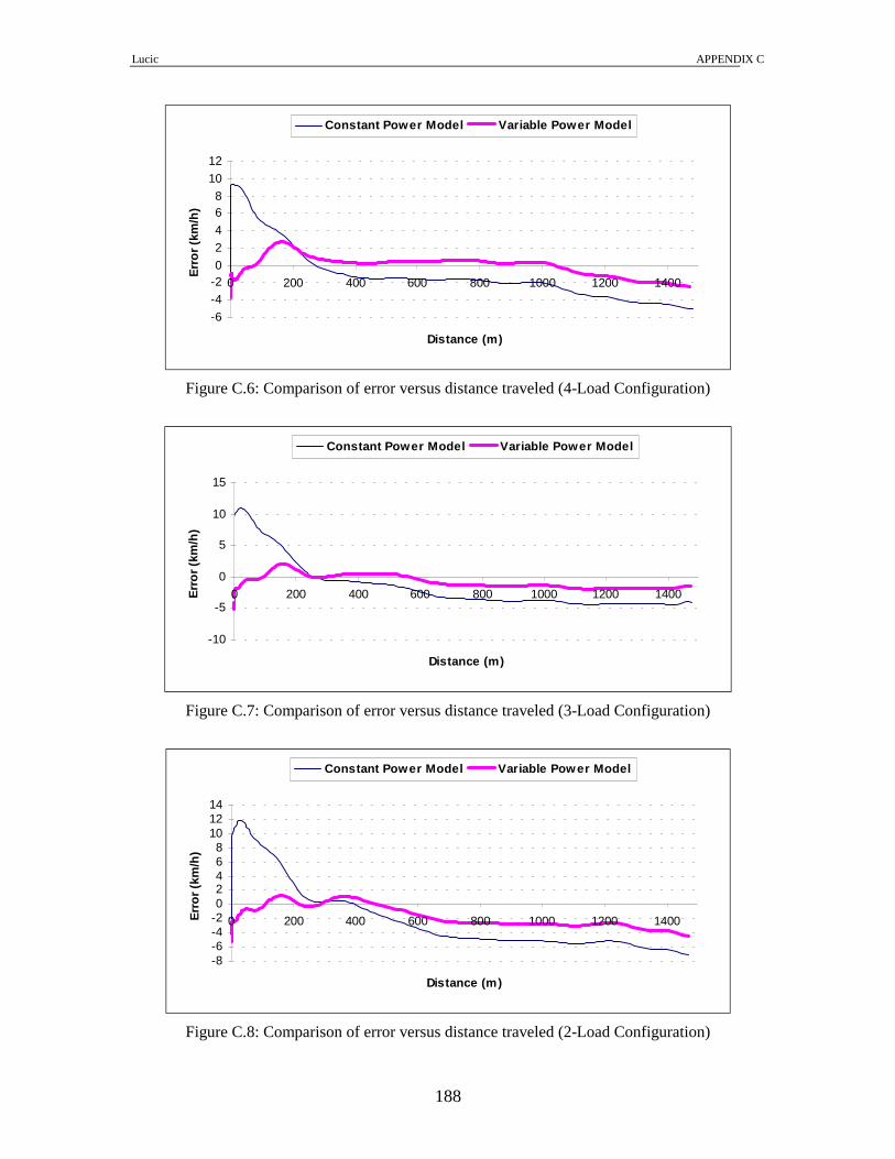
Lucic APPENDIX C
188
-6-4-202468
1012
0 200 400 600 800 1000 1200 1400
Distance (m)
Erro
r (km
/h)
Constant Power Model Variable Power Model
Figure C.6: Comparison of error versus distance traveled (4-Load Configuration)
-10
-5
0
5
10
15
0 200 400 600 800 1000 1200 1400
Distance (m)
Erro
r (km
/h)
Constant Power Model Variable Power Model
Figure C.7: Comparison of error versus distance traveled (3-Load Configuration)
-8-6-4-202468
101214
0 200 400 600 800 1000 1200 1400
Distance (m)
Erro
r (km
/h)
Constant Power Model Variable Power Model
Figure C.8: Comparison of error versus distance traveled (2-Load Configuration)

Lucic APPENDIX C
189
-10
-5
0
5
10
15
0 200 400 600 800 1000 1200 1400
Distance (m)
Erro
r (km
/h)
Constant Power Model Variable Power Model
Figure C.9: Comparison of error versus distance traveled (1-Load Configuration)
-8-6-4-202468
10121416
0 200 400 600 800 1000 1200 1400
Distance (m)
Erro
r (km
/h)
Basic Power Model Variable Power Model
Figure C.10: Comparison of error versus distance traveled (0-Load Configuration)

Lucic APPENDIX C
190
Truck with power of 320 kW (430 hp)
-4-202468
101214
0 200 400 600 800 1000 1200 1400
Distance (m)
Erro
r (km
/h)
Constant Power Model Variable Power Model
Figure C.11: Comparison of error versus distance traveled (9-Load Configuration)
-5
0
5
10
15
20
0 200 400 600 800 1000 1200 1400
Distance (m)
Erro
r (km
/h)
Constant Power Model Variable Power Model
Figure C.12: Comparison of error versus distance traveled (8-Load Configuration)
-5
0
5
10
15
0 200 400 600 800 1000 1200 1400
Distance (m)
Erro
r (km
/h)
Constant Power Model Variable Power Model
Figure C.13: Comparison of error versus distance traveled (7-Load Configuration)

Lucic APPENDIX C
191
-5
0
5
10
15
0 200 400 600 800 1000 1200 1400 1600
Distance (m)
Erro
r (km
/h)
Constant Power Model Variable Power Model
Figure C.14: Comparison of error versus distance traveled (6-Load Configuration)
-6-4-202468
101214
0 200 400 600 800 1000 1200 1400
Distance (m)
Erro
r (km
/h)
Constant Power Model Variable Power Model
Figure C.15: Comparison of error versus distance traveled (5-Load Configuration)
-6-4-202468
10121416
0 200 400 600 800 1000 1200 1400
Distance (m)
Erro
r (km
/h)
Constant Power Model Variable Power Model
Figure C.16: Comparison of error versus distance traveled (4-Load Configuration)

Lucic APPENDIX C
192
-5
0
5
10
15
20
0 200 400 600 800 1000 1200 1400
Distance (m)
Erro
r (km
/h)
Constant Power Model Variable Power Model
Figure C.17: Comparison of error versus distance traveled (3-Load Configuration)
-6-4-202468
1012141618
0 200 400 600 800 1000 1200 1400
Distance (m)
Erro
r (km
/h)
Constant Power Model Variable Power Model
Figure C.18: Comparison of error versus distance traveled (2-Load Configuration)
-8-6-4-202468
10121416
0 200 400 600 800 1000 1200 1400
Distance (m)
Erro
r (km
/h)
Constant Power Model Variable Power Model
Figure C.19: Comparison of error versus distance traveled (1-Load Configuration)

Lucic APPENDIX C
193
-4-202468
101214161820
0 200 400 600 800 1000 1200 1400
Distance (m)
Erro
r (km
/h)
Constant Power Model Variable Power Model
Figure C.20: Comparison of error versus distance traveled (0-Load Configuration)
-226
10141822263034
0 200 400 600 800 1000 1200 1400
Distance (m)
Erro
r (km
/h)
Constant Power Model Variable Power Model
Figure C.21: Comparison of error versus distance traveled (Truck Configuration)

Lucic APPENDIX C
194
Truck with power of 350 kW (470 hp)
-4-202468
101214
0 200 400 600 800 1000 1200 1400
Distance (m)
Erro
r (km
/h)
Constant Power Model Variable Power Model
Figure C.22: Comparison of error versus distance traveled (9–Load Configuration)
-4-202468
101214
0 200 400 600 800 1000 1200 1400
Distance (m)
Erro
r (km
/h)
Constant Power Model Variable Power Model
Figure C.23: Comparison of error versus distance traveled (8–Load Configuration)
-10
-5
0
5
10
15
0 200 400 600 800 1000 1200 1400
Distance (m)
Erro
r (km
/h)
Constant Power Model Variable Power Model
Figure C.24: Comparison of error versus distance traveled (7–Load Configuration)

Lucic APPENDIX C
195
-5
0
5
10
15
0 200 400 600 800 1000 1200 1400
Distance (m)
Erro
r (km
/h)
Constant Power Model Variable Power Model
Figure C.25: Comparison of error versus distance traveled (6–Load Configuration)
-5
0
5
10
15
0 200 400 600 800 1000 1200 1400
Distance (m)
Erro
r (km
/h)
Constant Power Model Variable Power Model
Figure C.26: Comparison of error versus distance traveled (5–Load Configuration)
-6-4-202468
10121416
0 200 400 600 800 1000 1200 1400
Distance (m)
Erro
r (km
/h)
Constant Power Model Variable Power Model
Figure C.27: Comparison of error versus distance traveled (4–Load Configuration)

Lucic APPENDIX C
196
-6-4-202468
10121416
0 200 400 600 800 1000 1200 1400
Distance(m)
Erro
r (km
/h)
Constant Power Model Variable Power Model
Figure C.28: Comparison of error versus distance traveled (3–Load Configuration)
-8-6-4-202468
101214
0 200 400 600 800 1000 1200 1400
Distance (m)
Erro
r (km
/h)
Constant Power Model Variable Power Model
Figure C.29: Comparison of error versus distance traveled (2–Load Configuration)
-8-6-4-202468
10121416
0 200 400 600 800 1000 1200 1400
Distance (m)
Erro
r (km
/h)
Constant Power Model Variable Power Model
Figure C.30: Comparison of error versus distance traveled (1–Load Configuration)

Lucic APPENDIX C
197
-4-202468
1012141618
0 200 400 600 800 1000 1200 1400
Distance (m)
Erro
r (km
/h)
Constant Power Model Variable Power Model
Figure C.31: Comparison of error versus distance traveled (0–Load Configuration)
-226
10141822263034
0 200 400 600 800 1000 1200 1400
Distance (m)
Erro
r (km
/h)
Constant Model Variable Model
Figure C.32: Comparison of error versus distance traveled (Truck Configuration)

Lucic APPENDIX C
198
Truck with power of 375 kW (500 hp)
-6-4-202468
1012
0 200 400 600 800 1000 1200 1400
Distance (m)
Erro
r (km
/h)
Constant Power Model Variable Power Model
Figure C.33: Comparison of error versus distance traveled (9–Load Configuration)
-5
0
5
10
15
0 200 400 600 800 1000 1200 1400
Distance (m)
Erro
r (km
/h)
Constant Power Model Variable Power Model
Figure C.34: Comparison of error versus distance traveled (8–Load Configuration)
-5
0
5
10
15
0 200 400 600 800 1000 1200 1400
Distance (m)
Erro
r (km
/h)
Constant Power Model Variable Power Model
Figure C.35: Comparison of error versus distance traveled (7–Load Configuration)

Lucic APPENDIX C
199
-10
-5
0
5
10
15
0 200 400 600 800 1000 1200 1400
Distance (m)
Erro
r (km
/h)
Constant Power Model Variable Power Model
Figure C.36: Comparison of error versus distance traveled (6–Load Configuration)
-6-4-202468
10121416
0 200 400 600 800 1000 1200 1400
Distance (m)
Erro
r (km
/h)
Constant Power Model Variable Power Model
Figure C.37: Comparison of error versus distance traveled (5–Load Configuration)
-6-4-202468
10121416
0 200 400 600 800 1000 1200 1400 1600
Distance (m)
Erro
r (km
/h)
Constant Power Model Variable Power Model
Figure C.38: Comparison of error versus distance traveled (4–Load Configuration)

Lucic APPENDIX C
200
-8-6-4-202468
101214
0 200 400 600 800 1000 1200 1400
Distance (m)
Erro
r (km
/h)
Constant Power Model Variable Power Model
Figure C.39: Comparison of error versus distance traveled (3–Load Configuration)
-8-6-4-202468
10121416
0 200 400 600 800 1000 1200 1400
Distance (m)
Erro
r (km
/h)
Constant Power Model Variable Power Model
Figure C.40: Comparison of error versus distance traveled (2–Load Configuration)
-8-6-4-202468
1012141618
0 200 400 600 800 1000 1200 1400
Distance (m)
Erro
r (km
/h)
Constant Power Model Variable Power Model
Figure C.41: Comparison of error versus distance traveled (1–Load Configuration)

Lucic APPENDIX C
201
-8-6-4-202468
1012141618
0 200 400 600 800 1000 1200 1400
Distance (m)
Erro
r (km
/h)
Constant Power Model Variable Power Model
Figure C.42: Comparison of error versus distance traveled (0–Load Configuration)

Lucic APPENDIX D
202
APPENDIX D

Lucic APPENDIX D
203
Mean mass variations for vehicle class 9 by DOW, direction, season and month for 3-year period
Table D.1: Mean mass (kg) variations by DOW, direction, season, and month for 1998 year DOW 1 mean = 24402.59 DOW 2 mean = 25045.53 DOW 3 mean = 24630.88 Direction 2 Direction 2 Direction 2 Season 1 Season 1 Season 1 Month 4 Month 4 Month 4 DOW 1 mean = 24110.36 DOW 2 mean = 25401.81 DOW 3 mean = 26132.61 Direction 2 Direction 2 Direction 2 Season 1 Season 1 Season 1 Month 5 Month 5 Month 5 DOW 1 mean = 24906.04 DOW 2 mean = 25251.59 DOW 3 mean = 25694.21 Direction 2 Direction 2 Direction 2 Season 1 Season 1 Season 1 Month 6 Month 6 Month 6 DOW 1 mean = 24764.09 DOW 2 mean = 25932.14 DOW 3 mean = 25677.29 Direction 2 Direction 2 Direction 2 Season 2 Season 2 Season 2 Month 7 Month 7 Month 7 DOW 1 mean = 25342.98 DOW 2 mean = 26127.12 DOW 3 mean = 26072.81 Direction 2 Direction 2 Direction 2 Season 2 Season 2 Season 2 Month 8 Month 8 Month 8 DOW 1 mean = 25233.22 DOW 2 mean = 26043.7 DOW 3 mean = 25935.51 Direction 2 Direction 2 Direction 2 Season 2 Season 2 Season 2 Month 9 Month 9 Month 9

Lucic APPENDIX D
204
Table D.1: Mean mass (kg) variations by DOW, direction, season, and month for 1998 year (Continued) DOW 4 mean = 24714.06 DOW 5 mean = 24439.52 DOW 6 mean = 25326.92 DOW 7 mean = 26455 Direction 2 Direction 2 Direction 2 Direction 2 Season 1 Season 1 Season 1 Season 1 Month 4 Month 4 Month 4 Month 4 DOW 4 mean = 25170.91 DOW 5 mean = 24750.33 DOW 6 mean = 26013.22 DOW 7 mean = 26791.64 Direction 2 Direction 2 Direction 2 Direction 2 Season 1 Season 1 Season 1 Season 1 Month 5 Month 5 Month 5 Month 5 DOW 4 mean = 25299.33 DOW 5 mean = 24669.53 DOW 6 mean = 24832.06 DOW 7 mean = 30476.64 Direction 2 Direction 2 Direction 2 Direction 2 Season 1 Season 1 Season 1 Season 1 Month 6 Month 6 Month 6 Month 6 DOW 4 mean = 25473.51 DOW 5 mean = 25154.02 DOW 6 mean = 26438.37 DOW 7 mean = 27108.28 Direction 2 Direction 2 Direction 2 Direction 2 Season 2 Season 2 Season 2 Season 2 Month 7 Month 7 Month 7 Month 7 DOW 4 mean = 25740.5 DOW 5 mean = 25131.54 DOW 6 mean = 26574.23 DOW 7 mean = 27594.96 Direction 2 Direction 2 Direction 2 Direction 2 Season 2 Season 2 Season 2 Season 2 Month 8 Month 8 Month 8 Month 8 DOW 4 mean = 25659.65 DOW 5 mean = 25275.92 DOW 6 mean = 26714.76 DOW 7 mean = 27569.38 Direction 2 Direction 2 Direction 2 Direction 2 Season 2 Season 2 Season 2 Season 2 Month 9 Month 9 Month 9 Month 9

Lucic APPENDIX D
205
Table D.2: Mean mass (kg) variations by DOW, direction, season, and month for 1999 year DOW 1 mean = 26475.16 DOW 2 mean = 27266.18 DOW 3 mean = 27418.97 Direction 1 Direction 1 Direction 1 Season 2 Season 2 Season 2 Month 9 Month 9 Month 9 DOW 1 mean = 23772.86 DOW 2 mean = 24500.36 DOW 3 mean = 24800.69 Direction 2 Direction 2 Direction 2 Season 1 Season 1 Season 1 Month 4 Month 4 Month 4 DOW 1 mean = 23752.37 DOW 2 mean = 24525.66 DOW 3 mean = 24352.73 Direction 2 Direction 2 Direction 2 Season 1 Season 1 Season 1 Month 5 Month 5 Month 5 DOW 1 mean = 23729.78 DOW 2 mean = 24486.53 DOW 3 mean = 24339.2 Direction 2 Direction 2 Direction 2 Season 1 Season 1 Season 1 Month 6 Month 6 Month 6 DOW 1 mean = 24594.5 DOW 2 mean = 25539.87 DOW 3 mean = 25285.89 Direction 2 Direction 2 Direction 2 Season 2 Season 2 Season 2 Month 7 Month 7 Month 7 DOW 1 mean = 24901.68 DOW 2 mean = 25893.4 DOW 3 mean = 25919.54 Direction 2 Direction 2 Direction 2 Season 2 Season 2 Season 2 Month 8 Month 8 Month 8 DOW 1 mean = 24920.86 DOW 2 mean = 25535.04 DOW 3 mean = 26219.75 Direction 2 Direction 2 Direction 2 Season 2 Season 2 Season 2 Month 9 Month 9 Month 9

Lucic APPENDIX D
206
Table D.2: Mean mass (kg) variations by DOW, direction, season, and month for 1999 year (Continued) DOW 4 mean = 27440.94 DOW 5 mean = 27446.99 DOW 6 mean = 29210.68 DOW 7 mean = 28527.09 Direction 1 Direction 1 Direction 1 Direction 1 Season 2 Season 2 Season 2 Season 2 Month 9 Month 9 Month 9 Month 9 DOW 4 mean = 24773.06 DOW 5 mean = 24044.16 DOW 6 mean = 25241.91 DOW 7 mean = 25796.55 Direction 2 Direction 2 Direction 2 Direction 2 Season 1 Season 1 Season 1 Season 1 Month 4 Month 4 Month 4 Month 4 DOW 4 mean = 24150.79 DOW 5 mean = 23243.3 DOW 6 mean = 24933.49 DOW 7 mean = 25713.93 Direction 2 Direction 2 Direction 2 Direction 2 Season 1 Season 1 Season 1 Season 1 Month 5 Month 5 Month 5 Month 5 DOW 4 mean = 23907.81 DOW 5 mean = 23424.46 DOW 6 mean = 24954.35 DOW 7 mean = 25501.9 Direction 2 Direction 2 Direction 2 Direction 2 Season 1 Season 1 Season 1 Season 1 Month 6 Month 6 Month 6 Month 6 DOW 4 mean = 25233.86 DOW 5 mean = 24895.98 DOW 6 mean = 25940.82 DOW 7 mean = 27077.76 Direction 2 Direction 2 Direction 2 Direction 2 Season 2 Season 2 Season 2 Season 2 Month 7 Month 7 Month 7 Month 7 DOW 4 mean = 25624.33 DOW 5 mean = 24929.64 DOW 6 mean = 26421.19 DOW 7 mean = 26910.36 Direction 2 Direction 2 Direction 2 Direction 2 Season 2 Season 2 Season 2 Season 2 Month 8 Month 8 Month 8 Month 8 DOW 4 mean = 25513.88 DOW 5 mean = 25675.3 DOW 6 mean = 27170.89 DOW 7 mean = 26707.09 Direction 2 Direction 2 Direction 2 Direction 2 Season 2 Season 2 Season 2 Season 2 Month 9 Month 9 Month 9 Month 9

Lucic APPENDIX D
207
Table D.3: Mean mass (kg) variations by DOW, direction, season, and month for 2000 year DOW 1 mean = 26194.73 DOW 2 mean = 26686.89 DOW 3 mean = 26812.68 Direction 1 Direction 1 Direction 1 Season 1 Season 1 Season 1 Month 5 Month 5 Month 5 DOW 1 mean = 26164.75 DOW 2 mean = 26590.6 DOW 3 mean = 26938.7 Direction 1 Direction 1 Direction 1 Season 1 Season 1 Season 1 Month 6 Month 6 Month 6 DOW 1 mean = 26774.46 DOW 2 mean = 26406.86 DOW 3 mean = 26646.86 Direction 1 Direction 1 Direction 1 Season 2 Season 2 Season 2 Month 7 Month 7 Month 7 DOW 1 mean = 26721.41 DOW 2 mean = 27185.62 DOW 3 mean = 27109.17 Direction 1 Direction 1 Direction 1 Season 2 Season 2 Season 2 Month 8 Month 8 Month 8 DOW 1 mean = 26622.78 DOW 2 mean = 27002.57 DOW 3 mean = 27142.55 Direction 1 Direction 1 Direction 1 Season 2 Season 2 Season 2 Month 9 Month 9 Month 9 DOW 1 mean = 23629.88 DOW 2 mean = 25319.09 DOW 3 mean = 25453.69 Direction 2 Direction 2 Direction 2 Season 1 Season 1 Season 1 Month 4 Month 4 Month 4 DOW 1 mean = 22950.27 DOW 2 mean = 24195.2 DOW 3 mean = 23823.47 Direction 2 Direction 2 Direction 2 Season 1 Season 1 Season 1 Month 5 Month 5 Month 5

Lucic APPENDIX D
208
Table D.3: Mean mass (kg) variations by DOW, direction, season, and month for 2000 year (Continued) DOW 1 mean = 25947.11 DOW 2 mean = 25551.83 DOW 3 mean = 25527.11 Direction 2 Direction 2 Direction 2 Season 1 Season 1 Season 1 Month 6 Month 6 Month 6 DOW 1 mean = 24022.27 DOW 2 mean = 24648.42 DOW 3 mean = 24241.67 Direction 2 Direction 2 Direction 2 Season 2 Season 2 Season 2 Month 7 Month 7 Month 7 DOW 1 mean = 24707.33 DOW 2 mean = 25555.53 DOW 3 mean = 25609.45 Direction 2 Direction 2 Direction 2 Season 2 Season 2 Season 2 Month 8 Month 8 Month 8 DOW 1 mean = 24115.41 DOW 2 mean = 24885.67 DOW 3 mean = 25071.14 Direction 2 Direction 2 Direction 2 Season 2 Season 2 Season 2 Month 9 Month 9 Month 9

Lucic APPENDIX D
209
Table D.3: Mean mass (kg) variations by DOW, direction, season, and month for 2000 year (Continued) DOW 4 mean = 26727.36 DOW 5 mean = 26196.84 DOW 6 mean = 27739.85 DOW 7 mean = 28183.45 Direction 1 Direction 1 Direction 1 Direction 1 Season 1 Season 1 Season 1 Season 1 Month 5 Month 5 Month 5 Month 5 DOW 4 mean = 27359.68 DOW 5 mean = 26440.04 DOW 6 mean = 27995.37 DOW 7 mean = 28135.16 Direction 1 Direction 1 Direction 1 Direction 1 Season 1 Season 1 Season 1 Season 1 Month 6 Month 6 Month 6 Month 6 DOW 4 mean = 26376.6 DOW 5 mean = 26427.14 DOW 6 mean = 27979.98 DOW 7 mean = 27892.42 Direction 1 Direction 1 Direction 1 Direction 1 Season 2 Season 2 Season 2 Season 2 Month 7 Month 7 Month 7 Month 7 DOW 4 mean = 27142.15 DOW 5 mean = 26059.08 DOW 6 mean = 27783.88 DOW 7 mean = 27908.82 Direction 1 Direction 1 Direction 1 Direction 1 Season 2 Season 2 Season 2 Season 2 Month 8 Month 8 Month 8 Month 8 DOW 4 mean = 26711.98 DOW 5 mean = 26199.52 DOW 6 mean = 27613.71 DOW 7 mean = 27964.32 Direction 1 Direction 1 Direction 1 Direction 1 Season 2 Season 2 Season 2 Season 2 Month 9 Month 9 Month 9 Month 9 DOW 4 mean = 24612.71 DOW 5 mean = 24315.79 DOW 6 mean = 25875.99 DOW 7 mean = 26656.88 Direction 2 Direction 2 Direction 2 Direction 2 Season 1 Season 1 Season 1 Season 1 Month 4 Month 4 Month 4 Month 4 DOW 4 mean = 23484.01 DOW 5 mean = 22494.42 DOW 6 mean = 23165.8 DOW 7 mean = 23270.63 Direction 2 Direction 2 Direction 2 Direction 2 Season 1 Season 1 Season 1 Season 1 Month 5 Month 5 Month 5 Month 5

Lucic APPENDIX D
210
Table D.3: Mean mass (kg) variations by DOW, direction, season, and month for 2000 year (Continued) DOW 4 mean = 25051.59 DOW 5 mean = 24264.78 DOW 6 mean = 25243.53 DOW 7 mean = 25494.08 Direction 2 Direction 2 Direction 2 Direction 2 Season 1 Season 1 Season 1 Season 1 Month 6 Month 6 Month 6 Month 6 DOW 4 mean = 24811.77 DOW 5 mean = 24609.67 DOW 6 mean = 24687.27 DOW 7 mean = 24805.91 Direction 2 Direction 2 Direction 2 Direction 2 Season 2 Season 2 Season 2 Season 2 Month 7 Month 7 Month 7 Month 7 DOW 4 mean = 25101.74 DOW 5 mean = 24781.33 DOW 6 mean = 25817.69 DOW 7 mean = 26477.83 Direction 2 Direction 2 Direction 2 Direction 2 Season 2 Season 2 Season 2 Season 2 Month 8 Month 8 Month 8 Month 8 DOW 4 mean = 24965.09 DOW 5 mean = 24155.96 DOW 6 mean = 25866.31 DOW 7 mean = 25942.31 Direction 2 Direction 2 Direction 2 Direction 2 Season 2 Season 2 Season 2 Season 2 Month 9 Month 9 Month 9 Month 9
Table D.4: Data Legend
DOW (Day of Week) Legend Direction Legend Season Legend Month Legend Monday 1 Northbound 1 Spring 1 April 4 Tuesday 2 Southbound 2 Summer 2 May 5 Wednesday 3 June 6 Thursday 4 July 7 Friday 5 August 8 Saturday 6 September 9 Sunday 7

Lucic APPENDIX D
211
Output results from SAS Results for DOW Number of observations 168 The SAS System 183 10:42 Wednesday, April 11, 2001 The GLM Procedure Dependent Variable: averageGVW Sum of Source DF Squares Mean Square F Value Pr > F Model 6 67962288.9 11327048.1 8.40 <.0001 Error 161 217066495.1 1348239.1 Corrected Total 167 285028784.0 R-Square Coeff Var Root MSE averageGVW Mean 0.238440 4.519961 1161.137 25689.09 Source DF Type I SS Mean Square F Value Pr > F dow 6 67962288.87 11327048.15 8.40 <.0001 The SAS System 184 10:42 Wednesday, April 11, 2001 The GLM Procedure Dependent Variable: averageGVW Source DF Type III SS Mean Square F Value Pr > F dow 6 67962288.87 11327048.15 8.40 <.0001 The SAS System 185 10:42 Wednesday, April 11, 2001 The GLM Procedure Level of ----------averageGVW--------- dow N Mean Std Dev 1 24 24948.2022 1116.70987 2 24 25649.0499 890.43597 3 24 25702.3565 1007.00586 4 24 25460.3050 1051.29071 5 24 24959.3849 1138.40712 6 24 26230.9269 1372.80950 7 24 26873.4332 1448.41531 The SAS System 186 10:42 Wednesday, April 11, 2001

Lucic APPENDIX D
212
Frequency ‚ ***** ‚ ***** ***** 40 ˆ ***** ***** ‚ ***** ***** ***** ‚ ***** ***** ***** ‚ ***** ***** ***** ***** 20 ˆ ***** ***** ***** ***** ‚ ***** ***** ***** ***** ‚ ***** ***** ***** ***** ***** ‚ ***** ***** ***** ***** ***** ***** Šƒƒƒƒƒƒƒƒƒƒƒƒƒƒƒƒƒƒƒƒƒƒƒƒƒƒƒƒƒƒƒƒƒƒƒƒƒƒƒƒƒƒƒƒƒƒƒƒƒƒƒƒƒƒƒƒƒƒƒƒƒƒƒƒƒ 22500 23500 24500 25500 26500 27500 28500 29500 30500 averageGVW Midpoint

Lucic APPENDIX D
213
Results for DIRECTION The SAS System 18:04 Tuesday, April 24, 2001 6 The GLM Procedure Class Level Information Class Levels Values direction 2 1 2 Number of observations 168 The SAS System 18:04 Tuesday, April 24, 2001 7 The GLM Procedure Dependent Variable: averageGVW Sum of Source DF Squares Mean Square F Value Pr > F Model 1 116898490.6 116898490.6 115.42 <.0001 Error 166 168130293.4 1012833.1 Corrected Total 167 285028784.0 R-Square Coeff Var Root MSE averageGVW Mean 0.410129 3.917601 1006.396 25689.09 Source DF Type I SS Mean Square F Value Pr > F direction 1 116898490.6 116898490.6 115.42 <.0001 Source DF Type III SS Mean Square F Value Pr > F direction 1 116898490.6 116898490.6 115.42 <.0001 The SAS System 18:04 Tuesday, April 24, 2001 8 The GLM Procedure Level of ----------averageGVW--------- direction N Mean Std Dev 1 42 27133.9031 733.95305 2 126 25207.4911 1080.90378 The SAS System 18:04 Tuesday, April 24, 2001 9

Lucic APPENDIX D
214
Frequency ‚ ***** ‚ ***** ‚ ***** ***** ‚ ***** ***** 40 ˆ ***** ***** ‚ ***** ***** ‚ ***** ***** ***** ‚ ***** ***** ***** ‚ ***** ***** ***** 30 ˆ ***** ***** ***** ‚ ***** ***** ***** ‚ ***** ***** ***** ‚ ***** ***** ***** ***** ‚ ***** ***** ***** ***** 20 ˆ ***** ***** ***** ***** ‚ ***** ***** ***** ***** ‚ ***** ***** ***** ***** ‚ ***** ***** ***** ***** ‚ ***** ***** ***** ***** ***** 10 ˆ ***** ***** ***** ***** ***** ‚ ***** ***** ***** ***** ***** ‚ ***** ***** ***** ***** ***** ‚ ***** ***** ***** ***** ***** ***** ‚ ***** ***** ***** ***** ***** ***** ***** ***** ***** Šƒƒƒƒƒƒƒƒƒƒƒƒƒƒƒƒƒƒƒƒƒƒƒƒƒƒƒƒƒƒƒƒƒƒƒƒƒƒƒƒƒƒƒƒƒƒƒƒƒƒƒƒƒƒƒƒƒƒƒƒƒƒƒƒƒƒƒƒƒƒƒƒƒƒƒƒƒƒƒƒƒƒƒƒƒ 22500 23500 24500 25500 26500 27500 28500 29500 30500 averageGVW Midpoint

Lucic APPENDIX D
215
Results for YEAR The SAS System 18:04 Tuesday, April 24, 2001 11 The GLM Procedure Class Level Information Class Levels Values year 3 1998 1999 2000 Number of observations 168 The SAS System 18:04 Tuesday, April 24, 2001 12 The GLM Procedure Dependent Variable: averageGVW Sum of Source DF Squares Mean Square F Value Pr > F Model 2 3170219.7 1585109.8 0.93 0.3974 Error 165 281858564.3 1708233.7 Corrected Total 167 285028784.0 R-Square Coeff Var Root MSE averageGVW Mean 0.011122 5.087739 1306.994 25689.09 Source DF Type I SS Mean Square F Value Pr > F year 2 3170219.683 1585109.842 0.93 0.3974 Source DF Type III SS Mean Square F Value Pr > F year 2 3170219.683 1585109.842 0.93 0.3974 The SAS System 18:04 Tuesday, April 24, 2001 13 The GLM Procedure Level of ----------averageGVW--------- year N Mean Std Dev 1998 42 25716.1609 1120.17057 1999 49 25482.5213 1320.81870 2000 77 25805.7858 1389.21371 The SAS System 18:04 Tuesday, April 24, 2001 14

Lucic APPENDIX D
216
Frequency ‚ ***** ‚ ***** ‚ ***** ***** ‚ ***** ***** 40 ˆ ***** ***** ‚ ***** ***** ‚ ***** ***** ***** ‚ ***** ***** ***** ‚ ***** ***** ***** 30 ˆ ***** ***** ***** ‚ ***** ***** ***** ‚ ***** ***** ***** ‚ ***** ***** ***** ***** ‚ ***** ***** ***** ***** 20 ˆ ***** ***** ***** ***** ‚ ***** ***** ***** ***** ‚ ***** ***** ***** ***** ‚ ***** ***** ***** ***** ‚ ***** ***** ***** ***** ***** 10 ˆ ***** ***** ***** ***** ***** ‚ ***** ***** ***** ***** ***** ‚ ***** ***** ***** ***** ***** ‚ ***** ***** ***** ***** ***** ***** ‚ ***** ***** ***** ***** ***** ***** ***** ***** ***** Šƒƒƒƒƒƒƒƒƒƒƒƒƒƒƒƒƒƒƒƒƒƒƒƒƒƒƒƒƒƒƒƒƒƒƒƒƒƒƒƒƒƒƒƒƒƒƒƒƒƒƒƒƒƒƒƒƒƒƒƒƒƒƒƒƒƒƒƒƒƒƒƒƒƒƒƒƒƒƒƒƒƒƒƒƒ 22500 23500 24500 25500 26500 27500 28500 29500 30500 averageGVW Midpoint

Lucic APPENDIX D
217
Results for SEASON The SAS System 18:04 Tuesday, April 24, 2001 22 The GLM Procedure Class Level Information Class Levels Values season 2 1 2 Number of observations 168 The SAS System 18:04 Tuesday, April 24, 2001 23 The GLM Procedure Dependent Variable: averageGVW Sum of Source DF Squares Mean Square F Value Pr > F Model 1 29548219.0 29548219.0 19.20 <.0001 Error 166 255480565.0 1539039.5 Corrected Total 167 285028784.0 R-Square Coeff Var Root MSE averageGVW Mean 0.103667 4.829210 1240.580 25689.09 Source DF Type I SS Mean Square F Value Pr > F season 1 29548218.97 29548218.97 19.20 <.0001 Source DF Type III SS Mean Square F Value Pr > F season 1 29548218.97 29548218.97 19.20 <.0001 The SAS System 18:04 Tuesday, April 24, 2001 24 The GLM Procedure Level of ----------averageGVW--------- season N Mean Std Dev 1 77 25233.1765 1385.99968 2 91 26074.8705 1102.95027 The SAS System 18:04 Tuesday, April 24, 2001 25

Lucic APPENDIX D
218
Frequency ‚ ***** ‚ ***** ‚ ***** ***** ‚ ***** ***** 40 ˆ ***** ***** ‚ ***** ***** ‚ ***** ***** ***** ‚ ***** ***** ***** ‚ ***** ***** ***** 30 ˆ ***** ***** ***** ‚ ***** ***** ***** ‚ ***** ***** ***** ‚ ***** ***** ***** ***** ‚ ***** ***** ***** ***** 20 ˆ ***** ***** ***** ***** ‚ ***** ***** ***** ***** ‚ ***** ***** ***** ***** ‚ ***** ***** ***** ***** ‚ ***** ***** ***** ***** ***** 10 ˆ ***** ***** ***** ***** ***** ‚ ***** ***** ***** ***** ***** ‚ ***** ***** ***** ***** ***** ‚ ***** ***** ***** ***** ***** ***** ‚ ***** ***** ***** ***** ***** ***** ***** ***** ***** Šƒƒƒƒƒƒƒƒƒƒƒƒƒƒƒƒƒƒƒƒƒƒƒƒƒƒƒƒƒƒƒƒƒƒƒƒƒƒƒƒƒƒƒƒƒƒƒƒƒƒƒƒƒƒƒƒƒƒƒƒƒƒƒƒƒƒƒƒƒƒƒƒƒƒƒƒƒƒƒƒƒƒƒƒƒ 22500 23500 24500 25500 26500 27500 28500 29500 30500 averageGVW Midpoint

Lucic APPENDIX D
219
Results for MONTH The SAS System 18:04 Tuesday, April 24, 2001 17 The GLM Procedure Class Level Information Class Levels Values month 6 4 5 6 7 8 9 Number of observations 168 The SAS System 18:04 Tuesday, April 24, 2001 18 The GLM Procedure Dependent Variable: averageGVW Sum of Source DF Squares Mean Square F Value Pr > F Model 5 43986049.4 8797209.9 5.91 <.0001 Error 162 241042734.5 1487918.1 Corrected Total 167 285028784.0 R-Square Coeff Var Root MSE averageGVW Mean 0.154321 4.748328 1219.802 25689.09 Source DF Type I SS Mean Square F Value Pr > F month 5 43986049.43 8797209.89 5.91 <.0001 Source DF Type III SS Mean Square F Value Pr > F month 5 43986049.43 8797209.89 5.91 <.0001 The SAS System 18:04 Tuesday, April 24, 2001 19 The GLM Procedure Level of ----------averageGVW--------- month N Mean Std Dev 4 21 24943.2439 800.51186 5 28 25034.5971 1537.58711 6 28 25649.2054 1510.83588 7 28 25694.5588 1079.07463 8 28 26112.3323 926.50284 9 35 26349.1505 1189.99400 The SAS System 18:04 Tuesday, April 24, 2001 20

Lucic APPENDIX D
220
Frequency ‚ ***** ‚ ***** ‚ ***** ***** ‚ ***** ***** 40 ˆ ***** ***** ‚ ***** ***** ‚ ***** ***** ***** ‚ ***** ***** ***** ‚ ***** ***** ***** 30 ˆ ***** ***** ***** ‚ ***** ***** ***** ‚ ***** ***** ***** ‚ ***** ***** ***** ***** ‚ ***** ***** ***** ***** 20 ˆ ***** ***** ***** ***** ‚ ***** ***** ***** ***** ‚ ***** ***** ***** ***** ‚ ***** ***** ***** ***** ‚ ***** ***** ***** ***** ***** 10 ˆ ***** ***** ***** ***** ***** ‚ ***** ***** ***** ***** ***** ‚ ***** ***** ***** ***** ***** ‚ ***** ***** ***** ***** ***** ***** ‚ ***** ***** ***** ***** ***** ***** ***** ***** ***** Šƒƒƒƒƒƒƒƒƒƒƒƒƒƒƒƒƒƒƒƒƒƒƒƒƒƒƒƒƒƒƒƒƒƒƒƒƒƒƒƒƒƒƒƒƒƒƒƒƒƒƒƒƒƒƒƒƒƒƒƒƒƒƒƒƒƒƒƒƒƒƒƒƒƒƒƒƒƒƒƒƒƒƒƒƒ 22500 23500 24500 25500 26500 27500 28500 29500 30500 averageGVW Midpoint

Lucic APPENDIX D
221
Results for DOW x DIRECTION Number of observations 168 The SAS System 356 10:42 Wednesday, April 11, 2001 The GLM Procedure Dependent Variable: averageGVW Sum of Source DF Squares Mean Square F Value Pr > F Model 13 187106578.1 14392813.7 22.64 <.0001 Error 154 97922205.9 635858.5 Corrected Total 167 285028784.0 R-Square Coeff Var Root MSE averageGVW Mean 0.656448 3.104070 797.4073 25689.09 Source DF Type I SS Mean Square F Value Pr > F dow*direction 13 187106578.1 14392813.7 22.64 <.0001 The SAS System 357 10:42 Wednesday, April 11, 2001 The GLM Procedure Dependent Variable: averageGVW Source DF Type III SS Mean Square F Value Pr > F dow*direction 13 187106578.1 14392813.7 22.64 <.0001 The SAS System 358 10:42 Wednesday, April 11, 2001 The GLM Procedure Level of Level of ----------averageGVW--------- dow direction N Mean Std Dev 1 1 6 26492.2108 262.77835 1 2 18 24433.5327 738.24028 2 1 6 26856.4525 346.16213 2 2 18 25246.5824 592.82196 3 1 6 27011.4863 272.22857 3 2 18 25265.9799 737.33583 4 1 6 26959.7852 419.57457 4 2 18 24960.4783 620.82204 5 1 6 26461.5997 504.67078 5 2 18 24458.6466 785.18152 6 1 6 28053.9098 585.20823 6 2 18 25623.2659 940.82127 7 1 6 28101.8773 240.26231 7 2 18 26463.9518 1453.00152 The SAS System 359 10:42 Wednesday, April 11, 2001
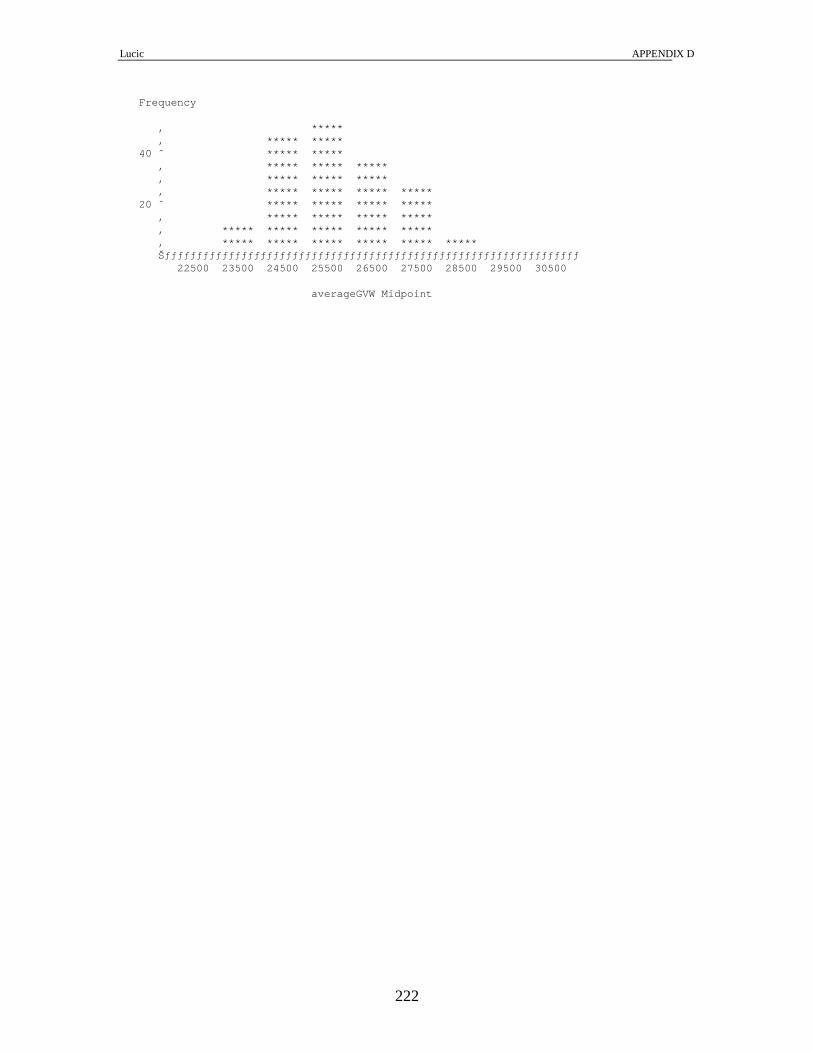
Lucic APPENDIX D
222
Frequency ‚ ***** ‚ ***** ***** 40 ˆ ***** ***** ‚ ***** ***** ***** ‚ ***** ***** ***** ‚ ***** ***** ***** ***** 20 ˆ ***** ***** ***** ***** ‚ ***** ***** ***** ***** ‚ ***** ***** ***** ***** ***** ‚ ***** ***** ***** ***** ***** ***** Šƒƒƒƒƒƒƒƒƒƒƒƒƒƒƒƒƒƒƒƒƒƒƒƒƒƒƒƒƒƒƒƒƒƒƒƒƒƒƒƒƒƒƒƒƒƒƒƒƒƒƒƒƒƒƒƒƒƒƒƒƒƒƒƒƒ 22500 23500 24500 25500 26500 27500 28500 29500 30500 averageGVW Midpoint

Lucic APPENDIX D
223
Results for DOW x DIRECTION, YEAR Number of observations 168 The SAS System 529 10:42 Wednesday, April 11, 2001 The GLM Procedure Dependent Variable: averageGVW Sum of Source DF Squares Mean Square F Value Pr > F Model 15 207653241.1 13843549.4 27.19 <.0001 Error 152 77375542.9 509049.6 Corrected Total 167 285028784.0 R-Square Coeff Var Root MSE averageGVW Mean 0.728534 2.777354 713.4771 25689.09 Source DF Type I SS Mean Square F Value Pr > F dow*direction 13 187106578.1 14392813.7 28.27 <.0001 year 2 20546663.0 10273331.5 20.18 <.0001 The SAS System 530 10:42 Wednesday, April 11, 2001 The GLM Procedure Dependent Variable: averageGVW Source DF Type III SS Mean Square F Value Pr > F dow*direction 13 204483021.4 15729463.2 30.90 <.0001 year 2 20546663.0 10273331.5 20.18 <.0001 The SAS System 531 10:42 Wednesday, April 11, 2001 The GLM Procedure Level of Level of ----------averageGVW--------- dow direction N Mean Std Dev 1 1 6 26492.2108 262.77835 1 2 18 24433.5327 738.24028 2 1 6 26856.4525 346.16213 2 2 18 25246.5824 592.82196 3 1 6 27011.4863 272.22857 3 2 18 25265.9799 737.33583 4 1 6 26959.7852 419.57457 4 2 18 24960.4783 620.82204 5 1 6 26461.5997 504.67078 5 2 18 24458.6466 785.18152 6 1 6 28053.9098 585.20823 6 2 18 25623.2659 940.82127 7 1 6 28101.8773 240.26231 7 2 18 26463.9518 1453.00152 The SAS System 532 10:42 Wednesday, April 11, 2001

Lucic APPENDIX D
224
The GLM Procedure Level of ----------averageGVW--------- year N Mean Std Dev 1998 42 25716.1609 1120.17057 1999 49 25482.5213 1320.81870 2000 77 25805.7858 1389.21371 The SAS System 533 10:42 Wednesday, April 11, 2001 Frequency ‚ ***** ‚ ***** ***** 40 ˆ ***** ***** ‚ ***** ***** ***** ‚ ***** ***** ***** ‚ ***** ***** ***** ***** 20 ˆ ***** ***** ***** ***** ‚ ***** ***** ***** ***** ‚ ***** ***** ***** ***** ***** ‚ ***** ***** ***** ***** ***** ***** Šƒƒƒƒƒƒƒƒƒƒƒƒƒƒƒƒƒƒƒƒƒƒƒƒƒƒƒƒƒƒƒƒƒƒƒƒƒƒƒƒƒƒƒƒƒƒƒƒƒƒƒƒƒƒƒƒƒƒƒƒƒƒƒƒƒ 22500 23500 24500 25500 26500 27500 28500 29500 30500 averageGVW Midpoint

Lucic APPENDIX D
225
Results for DOW x DIRECTION, YEAR, MONTH Number of observations 168 The SAS System 703 10:42 Wednesday, April 11, 2001 The GLM Procedure Dependent Variable: averageGVW Sum of Source DF Squares Mean Square F Value Pr > F Model 20 229940776.7 11497038.8 30.68 <.0001 Error 147 55088007.3 374748.3 Corrected Total 167 285028784.0 R-Square Coeff Var Root MSE averageGVW Mean 0.806728 2.382984 612.1669 25689.09 Source DF Type I SS Mean Square F Value Pr > F dow*direction 13 187106578.1 14392813.7 38.41 <.0001 year 2 20546663.0 10273331.5 27.41 <.0001 month 5 22287535.6 4457507.1 11.89 <.0001 The SAS System 704 10:42 Wednesday, April 11, 2001 The GLM Procedure Dependent Variable: averageGVW Source DF Type III SS Mean Square F Value Pr > F dow*direction 13 181504202.3 13961861.7 37.26 <.0001 year 2 19114217.2 9557108.6 25.50 <.0001 month 5 22287535.6 4457507.1 11.89 <.0001 The SAS System 705 10:42 Wednesday, April 11, 2001 The GLM Procedure Level of Level of ----------averageGVW--------- dow direction N Mean Std Dev 1 1 6 26492.2108 262.77835 1 2 18 24433.5327 738.24028 2 1 6 26856.4525 346.16213 2 2 18 25246.5824 592.82196 3 1 6 27011.4863 272.22857 3 2 18 25265.9799 737.33583 4 1 6 26959.7852 419.57457 4 2 18 24960.4783 620.82204 5 1 6 26461.5997 504.67078 5 2 18 24458.6466 785.18152 6 1 6 28053.9098 585.20823 6 2 18 25623.2659 940.82127 7 1 6 28101.8773 240.26231

Lucic APPENDIX D
226
7 2 18 26463.9518 1453.00152 The SAS System 706 10:42 Wednesday, April 11, 2001 The GLM Procedure Level of ----------averageGVW--------- year N Mean Std Dev 1998 42 25716.1609 1120.17057 1999 49 25482.5213 1320.81870 2000 77 25805.7858 1389.21371 Level of ----------averageGVW--------- month N Mean Std Dev 4 21 24943.2439 800.51186 5 28 25034.5971 1537.58711 6 28 25649.2054 1510.83588 7 28 25694.5588 1079.07463 8 28 26112.3323 926.50284 9 35 26349.1505 1189.99400 The SAS System 707 10:42 Wednesday, April 11, 2001 Frequency ‚ ***** ‚ ***** ***** 40 ˆ ***** ***** ‚ ***** ***** ***** ‚ ***** ***** ***** ‚ ***** ***** ***** ***** 20 ˆ ***** ***** ***** ***** ‚ ***** ***** ***** ***** ‚ ***** ***** ***** ***** ***** ‚ ***** ***** ***** ***** ***** ***** Šƒƒƒƒƒƒƒƒƒƒƒƒƒƒƒƒƒƒƒƒƒƒƒƒƒƒƒƒƒƒƒƒƒƒƒƒƒƒƒƒƒƒƒƒƒƒƒƒƒƒƒƒƒƒƒƒƒƒƒƒƒƒƒƒƒ 22500 23500 24500 25500 26500 27500 28500 29500 30500 averageGVW Midpoint

Lucic APPENDIX D
227
Results for DOW x DIRECTION, YEAR, SEASON Number of observations 168 The SAS System 1051 10:42 Wednesday, April 11, 2001 The GLM Procedure Dependent Variable: averageGVW Sum of Source DF Squares Mean Square F Value Pr > F Model 16 221905333.9 13869083.4 33.18 <.0001 Error 151 63123450.0 418036.1 Corrected Total 167 285028784.0 R-Square Coeff Var Root MSE averageGVW Mean 0.778537 2.516854 646.5571 25689.09 Source DF Type I SS Mean Square F Value Pr > F dow*direction 13 187106578.1 14392813.7 34.43 <.0001 year 2 20546663.0 10273331.5 24.58 <.0001 season 1 14252092.8 14252092.8 34.09 <.0001 The SAS System 1052 10:42 Wednesday, April 11, 2001 The GLM Procedure Dependent Variable: averageGVW Source DF Type III SS Mean Square F Value Pr > F dow*direction 13 188570030.0 14505386.9 34.70 <.0001 year 2 19502438.3 9751219.2 23.33 <.0001 season 1 14252092.8 14252092.8 34.09 <.0001 The SAS System 1053 10:42 Wednesday, April 11, 2001 The GLM Procedure Level of Level of ----------averageGVW--------- dow direction N Mean Std Dev 1 1 6 26492.2108 262.77835 1 2 18 24433.5327 738.24028 2 1 6 26856.4525 346.16213 2 2 18 25246.5824 592.82196 3 1 6 27011.4863 272.22857 3 2 18 25265.9799 737.33583 4 1 6 26959.7852 419.57457 4 2 18 24960.4783 620.82204 5 1 6 26461.5997 504.67078 5 2 18 24458.6466 785.18152 6 1 6 28053.9098 585.20823 6 2 18 25623.2659 940.82127 7 1 6 28101.8773 240.26231 7 2 18 26463.9518 1453.00152

Lucic APPENDIX D
228
The SAS System 1054 10:42 Wednesday, April 11, 2001 The GLM Procedure Level of ----------averageGVW--------- year N Mean Std Dev 1998 42 25716.1609 1120.17057 1999 49 25482.5213 1320.81870 2000 77 25805.7858 1389.21371 Level of ----------averageGVW--------- season N Mean Std Dev 1 77 25233.1765 1385.99968 2 91 26074.8705 1102.95027 The SAS System 1055 10:42 Wednesday, April 11, 2001 Frequency ‚ ***** ‚ ***** ***** 40 ˆ ***** ***** ‚ ***** ***** ***** ‚ ***** ***** ***** ‚ ***** ***** ***** ***** 20 ˆ ***** ***** ***** ***** ‚ ***** ***** ***** ***** ‚ ***** ***** ***** ***** ***** ‚ ***** ***** ***** ***** ***** ***** Šƒƒƒƒƒƒƒƒƒƒƒƒƒƒƒƒƒƒƒƒƒƒƒƒƒƒƒƒƒƒƒƒƒƒƒƒƒƒƒƒƒƒƒƒƒƒƒƒƒƒƒƒƒƒƒƒƒƒƒƒƒƒƒƒƒ 22500 23500 24500 25500 26500 27500 28500 29500 30500 averageGVW Midpoint

Lucic VITA
229
VITA
Name Ivana Lucic
Place and Year of Birth Belgrade, Yugoslavia, 1967
Education Faculty of Traffic and Transportation Engineering,
University of Belgrade, Bachelor of Science, 1993
Experience Yugoslav Airlines, Belgrade, Yugoslavia, 1994-1999
Publication Rakha H., Lucic I., Demarchi S., Setti J., and Van Aerde
M. (2001), Vehicle Dynamics Model for Predicting
Maximum Vehicle Acceleration Levels, Accepted for
publication in the ASCE Journal of Transportation
Engineering.


![[Megafileupload]Euklidska i Hiperbolicka Geometrija - Zoran Lucic](https://img.dokumen.tips/doc/110x75/55cf9db9550346d033aee8ea/megafileuploadeuklidska-i-hiperbolicka-geometrija-zoran-lucic.jpg)