1  

Author version: J. Mar. Syst., vol.115-116; 2013; 40-61

Trophic Efficiency of Plankton Food Webs: Observations from the Gulf of Mannar and the Palk Bay, Southeast Coast of India

Anjusha, A1., *Jyothibabu, R1., Jagadeesan, L1., Arya P. Mohan1, Sudheesh, K2., Kiran Krishna1., Ullas, N1., Deepak, M.P1

1CSIR- National Institute of Oceanography, Regional Centre, Kochi – 682018 2CSIR- National Institute of Oceanography, Dona Paula, Goa – 403 004

*Corresponding author, E mail: rjyothibabu@nio.org, Telephone: 091 484 2390814, Fax: 091 484 390618

-------------------------------------------------------------------------------------------------------------------------------------------------------- Abstract

This paper introduces the structure and trophic efficiency of plankton food webs in the Gulf of Mannar (GoM) and the Palk Bay (PB) - two least studied marine environments located between India and Sri Lanka. The study is based on results obtained from a field sampling exercise carried out in the GoM and the PB in March 2010 (Spring Intermonsoon - SIM), September 2010 (Southwest Monsoon - SWM) and January 2011 (Northeast Monsoon - NEM). Based on multivariate analysis of major environmental parameters during different seasons, it was possible to clearly segregate the GoM and the PB into separate clusters, except during the SWM. This segregation of the GoM and the PB was closely linked with the seasonally reversing ocean currents in the region, as evident from the MIKE 21 flow model results. During the period of relatively low phytoplankton biomass (<23 mg C m-3), the organic carbon contribution of the microbial loop was significantly high - both in the GoM and the PB. During the SIM, the carbon biomass available in the plankton food web was significantly higher in the PB (av. 122.8 ± 47.60 mg C m-3) than in the GoM (av. 81.89 ± 35.50 mg C m-3). This was due to a strong microbial loop in the former region. In the GoM, phytoplankton contributed a considerable portion (>50%) of the carbon biomass during the SWM and the NEM, whereas, microbial loop contributed significantly (80%) during the SIM. The microbial loop was predominant in the PB throughout the study period, being as high as 83% of the total plankton biomass during the SIM. As compared to the PB, the mesozooplankton biomass was higher in the GoM during the SWM and the NEM and lower during the SIM. The relatively high mesozooplankton stock in the PB during the SIM was closely linked with a strong microbial loop, which contributed the major share (av. 101.6 ± 24.3 mg C m-3) of the total organic carbon available in the food web (av. 126.6 ± 24.3 mg C m-3). However, when microbial loop contributed >65% of the total organic carbon available in the food web, the trophic efficiency was found to be low (~3%), which can be attributed to the wide dispersal of organic carbon in the microbial loop. Importantly, during the NEM, when the copepod Paracalanus parvus was predominant in the PB, the trophic efficiency of the microbial loop dominant food web increased by more than a fold (7.2%).The study provides evidences for the first time from the field that exceptionally high abundance of efficient microzooplankton-consuming zooplankton can significantly increase the trophic efficiency of the microbial loop dominant plankton food web. -------------------------------------------------------------------------------------------------------------------------------------------------------- Key Words: Plankton, Food webs, Zooplankton, Multivariate analysis, Fluorescence microscopy, Arabian Sea, Bay of Bengal

2  

1. Introduction

Autotrophs produce new particulate matter in marine environments, which gets transferred to the high trophic levels through two major pathways (a) traditional and (b) microbial. The traditional food web begins from phytoplankton and transfers organic carbon from the primary producers to the high trophic levels (Riley, 1947). On the other hand, the microbial food web consists of organisms, which transfers organic carbon from smaller autotrophs and heterotrophic bacteria to higher trophic levels. These smaller organisms involved in the microbial food web include both autotrophic and heterotrophic forms of picoplankton (<2 μm) and nanoplankton (2 - 20 μm). Most of this picoplankton and nanoplankton carbon biomass is channeled to the higher trophic levels through the microzooplankton (20 – 200 µm), and this lateral link of the plankton food web is known as ‘microbial loop’ (Azam et al., 1983). Across the world, considerable scientific effort has been dedicated in the recent years to understand the plankton food web. A common feature evident in these studies is the dominance of the traditional food web in productive waters and that of the microbial food web in oligotrophic waters (Sherr and Sherr, 1988; Cushing, 1989).

To understand the sustenance of higher trophic levels in marine ecosystems, it is essential to improve our knowledge of the relative trophic importance of various plankton components (Cho and Azam., 1990). In recent years, the microbial loop has been recognized as an ecologically relevant trophic pathway, which potentially connects the carbon biomass of microbes with higher trophic levels. Pomeroy et al., (2007) proved that microbes dominate the energy flux of biologically relevant chemicals in the oceans, which is estimated to be five to ten times higher than the mass of all multi-cellular marine organisms. Research during the recent decades also indicated that the trophic transfer efficiency of the microbial loop is significantly low due to the wide dispersal of organic carbon in several intermediate trophic levels (Cushing, 1989; Berglund et al., 2007). However, Pomeroy et al., (1999 a) presented their view that the actual amount of carbon flux from smaller plankton to higher trophic levels depend on several factors, which include the assimilation efficiency, length of the food chains, chemical and physical nature of the available organic carbon, connectivity and retentiveness. Under the JGOFS program, comprehensive studies on various plankton components have been carried out in the central and western Arabian Sea, which show noticeable seasonal and spatial differences in the distribution of various plankton components (Garisson et al., 2000).

The present study analyses the plankton food web structure and organic carbon distribution in various plankton components in two least studied marine environments in the northern Indian Ocean, the Gulf of Mannar (GoM) and the Palk Bay (PB). The GoM is connected to the Arabian Sea (AS) in the west and the Palk Bay (PB) to the Bay of Bengal (BoB) in the east (Figure 1a). The Rameswaram (Pamban) island of India, Ramsethu (Adam’s Bridge) and Mannar Island of Sri Lanka are the physical barriers that inhibit the exchange of waters between the GoM and the PB (Figure 1b). Considering this unique geographic setting of the GoM and the PB, we assumed measurable level differences in the plankton food web structure and availability of organic carbon in the microbial loop in these regions. In order to verify this assumption, we conducted field sampling sessions in the GoM and the PB for three seasons, with the following objectives in mind: (a) to delineate the plankton food web structure (b) to understand the relative distribution of organic carbon in the traditional plankton food web (phytoplankton - zooplankton), microbial loop (heterotrophic bacteria - heterotrophic nanoplankton – microzooplankton -

3  

mesozooplankton) and integrated plankton food web (traditional + microbial) (c) to understand the distribution ecology of various plankton components in the food web and (d) to realize the interrelationship between the microbial loop and mesozooplankton especially the copepods.

2. Materials and methods

2.1. Study area

The GoM and the PB are geographically distinct and oceanographically least studied environments located between India and Sri Lanka (Figure 1a). To the western side of the GoM lies the high saline Arabian Sea and on the eastern side of the PB is the low saline Bay of Bengal. The physical barriers Rameswaram (Pamban) island of India, Ram Sethu (Adam’s Bridge) and Mannar Island of Sri Lanka partially separate the GoM and the PB. The ocean currents around the Indian subcontinent undergo seasonal reversal where the West India Coastal Current (WICC) and the Summer Monsoon Current (SMC) bring salty Arabian Sea waters into the Bay of Bengal during the SWM (Vinayachandran et al., 1999; Figure 2a). On the other hand, the East India Coastal Current (EICC) and Winter Monsoon Current (WMC) carry low saline Bay of Bengal waters in to the Arabian Sea during the NEM (Shankar et al., 2002).

The GoM extends ~190 km along the Indian coastline with an area of ~19600 km2. It is a Marine Biosphere Reserve endowed with rich and diverse living resources including several commercially important pelagic fishes. There are 21 coral islands in the Indian sector of the GoM, which have been declared as a Marine National Park. Though the GoM has a tropical climate, the contribution of the SWM to the annual rainfall in this region is only trivial. Most of the rainfall is received during the early NEM, when northeasterly winds blow over the region. However, the GoM seems to be influenced by both the SWM and the NEM ocean circulation and hence has a unique hydrography (Rao et al., 2008). Rivers Tamiraparani, Gundar, Vembar, and Vaippar drain into the GoM, but they are non-perennial rivers and carry appreciable amount of waters only during the NEM period.

The PB is a shallow flat basin (av. depth 9m), which extends ~260 km along the Indian coastline with an area of ~13500 km2. The PB is known for diverse biological resources present in the seagrass beds in regions where water column is shallow, and the bottom substratum is sandy or silty (Sridhar et al., 2010; Manikandan et al., 2011). During the NEM, the PB receives large amounts of suspended sediments from the BoB and acts as their reservoir (Chandramohan et al., 2001). Under the influence of low wave action, the high level of suspended sediments in the PB causes the deposition and emergence of sand banks (Chandramohan et al., 2001). The seasonal rainfall pattern in the PB is similar to the GoM with moderate to heavy rain fall during the early NEM. Similar to the GoM, both the SWM and the NEM ocean currents influence the hydrography of the PB. However, the biological responses of the GoM and the PB seem to be different, which has been attributed to their difference in depth and distribution of suspended sediments (Rao et al., 2008).

4  

2.2. Sampling and methods

Sampling was carried out in the GoM and the PB in March 2010 (SIM), September 2010 (SWM) and January 2011 (NEM). Field sampling was carried out in 30 locations distributed in 10 transects with 15 locations each in the GoM and the PB (Figure 1a). Water samples were collected using Niskin samplers from 2 depths (surface and bottom waters) for measuring dissolved oxygen and biological parameters. Turbidity in the study area was measured as per the nephelometric principles, using a turbidity meter. The climate in the GoM and the PB are presented from (a) air temperature data from AWS installed at Mandapam and (b) the mean rainfall data for the last five years (IMD, Pune) for the districts of Tuticorin, Ramnathapuram and Nagapattinam. The vertical salinity and temperature structure were recorded using a portable CTD profiler. The synoptic picture of the currents and estimations of exchange of waters between the GoM and the PB were made using model simulations. The circulation in the GoM and the PB has been simulated with MIKE 21 FM model. The model has been validated with currents measurements using RCM9 current meters deployed at selected locations in the study area (Figure 1a). The model simulations and actual field measurements of currents showed significant positive correlations (Sudheesh et al., 2013 for details). Due to uneven bathymetry of the study area, the bottom sampling depths in various locations are different, especially when locations in the GoM and the PB are compared. This difference in bottom sampling depths can introduce certain level of error in interpretations when bottom parameters are compared between the GoM and the PB. In order to minimize this error factor, comparison of bottom parameters between the GoM and the PB locations has been avoided throughout this paper. However, it is important to note that the surface and bottom sampling depths in both the GoM and the PB are actually present within the surface mixed layer (within the upper 15m). Therefore, most of the hydrographical parameters, except turbidity and dissolved oxygen, show only slight differences between the surface and bottom waters (Table 1).

2.2.1. Dissolved oxygen and chlorophyll a

The dissolved oxygen samples were fixed onboard and estimated following Winkler’s method (Grasshoff et al., 1983). Water samples (1L) were filtered through Whatman GF/F filter papers and the chlorophyll a present in the phytoplankton cells was extracted in 90% acetone and measured using a calibrated Turner designed flourometer (UNESCO, 1994). The chlorophyll a concentration was converted to equivalent organic carbon biomass using suitable conversion factors. Since the study area was in the inshore waters along the southeast coast of India, a factor of 25 was used to convert chlorophyll a into equivalent carbon biomass (Anita et al., 1963; Jonge, 1980; Shiyomoto et al., 1997). Our simultaneous study to understand the organic carbon content of autotrophic pico- and nanoplankton in the GoM and the PB showed that a factor of 25 is suitable to convert the chlorophyll a to equivalent carbon biomass and the values obtained so, had >90% accuracy when compared with the results obtained from the biovolume estimation methods (Jyothibabu et al., 2013).

5  

2.2.2. Picoplankton and Nanoplankton

Epiflourescence microscope was used to quantify the abundance of picoplankton and nanoplankton in the study area. Water samples (20 ml) were collected and carefully transferred into sterilized dark polyethylene bottles and preserved in 1% final concentration of gluteraldehyde and stored in cool temperature. In the laboratory, part of the sample (10 ml) was prefiltered through 3µm pore sized sterile filters and removed larger organisms and debris. The autotrophic and heterotrophic picoplankton were quantified using 2 sets of prefiltered samples in duplicate, using fluorescence microscopy. One set was processed for heterotrophic picoplankton by staining the samples with DAPI (Porter and Feig, 1980), and the other set was directly processed without any staining procedure. These two sets of samples were then filtered separately into 0.2 µm black nucleopore filters (25 mm diameter) and mounted in immersion oil for examining under an Olympus BX 53 epiflourescence microscope equipped with an image analyzer (progRes Capture Pro 2.6). The DAPI stained slides were examined under UV excitation while the unstained slides were observed under blue excitation. Blue fluorescent heterotrophic bacteria and red or orange auto-fluorescent picoautotrophs were counted and documented. However, due to weak fluorescence of autotrophic picoplankton during the SIM caused by inadequate preservation, the autotrophic picoplankton data for that particular season has not been presented in this paper. The carbon biomass of the heterotrophic picoplankton was estimated using standard conversion factor of 0.011pgC cell−1 (Garrison et al., 2000).

Water samples (20 ml) were passed through 20 µm sieve to remove larger organisms and debris and fixed in gluteraldehyde. The fixed samples (30 ml) were used for measuring the autotrophic and heterotrophic nanoplankton. Water samples (5 ml) in duplicates were stained with 1.65 µg ml-1 of proflavin hemisulfate and filtered through 25 mm diameter 0.8 µm black polycarbonate membrane filters (Haas, 1982). The membranes were mounted in Olympus immersion oil and examined under an epiflourescence microscope (Olympus BX 53) under blue excitation. All cells with body dimension 2 to 20µm that fluoresced green were counted as heterotrophic nanoplankton. As proflavin does not interfere with the chlorophyll auto-fluorescence, the phototrophs on the filters were distinguished from the heterotrophs based on their red /orange fluorescence. The cell dimensions of around 250 individuals of heterotrophic nanoplankton were randomly measured from the filters, using the image analyzer. Their biovolume was calculated by assuming suitable geometrical shapes (Garrison et al., 2000). The carbon biomass of the heterotrophic nanoplankton was calculated based on the cell volume measurements and subsequent conversion into equivalent carbon using the formula log10 C = 0.94 (log10 V) - 0.60 (Garrison et al., 2000). However, as in the case of autotrophic picoplankton, the autoflourescence of nanoplankton was very feeble during the SIM period and hence the data for the period has not been presented in this paper.

2.2.3. Microzooplankton

One liter water samples were collected in black polythene bottles and fixed in 3% acid Lugol’s iodine. The samples were concentrated by gravity settling into 20 ml. One day before the microscopic analysis, the samples were allowed to settle and concentrated in a settling chamber. Around 50 fields of view were randomly imaged under the inverted microscope (Olympus 1X 71) equipped with an image analyzer. The entire MZP samples were imaged with in a fortnight period of the

6  

sampling so as to minimize any kind of shrinkage due to preservation. The organisms captured in the images were identified and categorized into various groups such as ciliates, heterotrophic dinoflagellates, and the copepod nauplii. Ciliates and heterotrophic dinoflagellates were identified up to the species level following standard literature (Kofoid and Campell, 1939; Steidinger and Williams, 1970; Subrahmanyan, 1971; Taylor 1976 a, b; Tomas, 1997; Kalavati and Raman, 2008). The biovolume of ciliates and heterotrophic dinoflagellates were estimated using an image analyzer, and their organic carbon content was calculated by adopting standard conversion factors (UNESCO, 1994). The organic carbon content of the copepod nauplii was also estimated using standard conversion factor available in literature (UNESCO, 1994).

2.2.4. Mesozooplankton

Mesozooplankton was sampled using a WP net with a mouth area of 0.3 m2 and a mesh size 200 µm. The net was operated horizontally just below the water surface (~1m depth) with a flow meter (Hydro-bios) attached across the mouth. All zooplankton collections were carried out during the day time to minimize the possible error in biomass estimations due to vertical migration of zooplankton. The biomass was measured by the displacement volume method (Postel et al. 2000) and the samples were then preserved in 4% formalin in seawater for further analysis. Sub-samples (50%) of the zooplankton were made using a Folsom splitter and sorted into various taxonomic groups. The abundance of each group was calculated as per the standard procedure (Postel et al., 2000). Copepods were identified down to the species level based on standard literature (Tanaka 1956; Kasturirangan 1963; Sewell, 1999; Conway et al., 2003). However, the relevant zooplankton data to explain the food web structure is only presented in this paper and detailed information on mesozooplankton community in the study area available in Jagadeesan et al., (2013). The displacement volume of the zooplankton was converted to organic carbon using suitable conversion factors (Madhupratap et al., 1996; Padmavati et al., 1998).

2.2.5. Statistical Analyses

Multivariate analyses of clustering and NMDS were used to segregate the environmental data into clusters based on their similarity. The data or locations in one cluster indicate their similarity or homogeneity whereas their segregation into different clusters shows their dissimilarity or heterogeneity. The environmental parameters were initially standardized, and square root transformed to normalize the data (Clark and Warwick, 2001). Euclidean distance similarity index based group average linking was used for the spatial grouping of locations. In addition to the cluster analysis, Similarity Profile (SIMPROF) permutation test (Clarke and Gorley, 2006) was also performed to identify the significant assemblages of locations (P< 0.05). The Shannon and Weaver diversity index (H’) is used to measure the species diversity, which takes into account the richness and evenness of species (Shannon and Weaver, 1949). Redundancy analysis (RDA) was carried out to understand the ecological relationships between different biological variables and environmental parameters. Detrended Correspondence Analysis (DCA) was performed initially to select the suitable ordination techniques for the present data set. The resulting DCA showed axis gradient lengths of < 2, which means that the linear multivariate method of redundancy analyses with species correlations and scaling ordination scores is suitable for the current data (Ter- Braak and Smilauer, 1998; Leps and Smilauer,

7  

2003). Biological variables were log transformed and centered prior to the analysis, and the ordination significance was tested with Monte Carlo permutation tests (499 unrestricted permutations) for significance (p < 0.05).

In order to understand the top down control (grazing) of zooplankton on various components of the plankton food web, the dominant species of copepods in the study area were found out as per standard procedures (Yang et al., 1999; Lee et al., 2009, Lin et al., 2011)

Yi = (Ni / N) × fi

Where, Yi is the dominance of species i, Ni is the number of individuals of species i in all locations, N is the number of individuals of all species in all locations, and fi is the frequency of locations at which species i occurs. Species of copepods with a Y value ≥ 0.02 were defined as dominant species (Yang et al., 1999, Lee et al., 2009, Lin et al., 2011). The abundance data of the dominant copepods were included in the RDA analyses and Triplots to understand their spatial distribution and relationship with various plankton components in the food web.

3. Results

3.1. Air temperature, Rainfall and Surface currents

The monthly mean air temperature and rainfall in the study area is presented in Figure 2b. The air temperature shows a rising trend from January (25.5 °C) to May (30.5°C) and then a decrease towards December (25.9). Rainfall in the study region mostly occurs during the October - December period under the spell of the NEM. The contribution of the SWM to the annual rainfall in the region is very minor (Figure 2b). The spatial trend in rainfall showed an increasing trend from west to east, which was about 802 mm, 1033 mm and 1605 mm respectively in the Tuticorin, Ramnathapuram and Nagapattinam districts.

Seasonally reversing ocean currents were prevalent in the study area (Figure 3). The currents were weaker during the NEM and the SIM as compared to the SWM. During the NEM, weak currents were oriented from the PB to the GoM. During all the seasons, stronger currents were present in the channels across the physical barriers (Pamban and Ramsethu). The currents were strongest during the SWM and weakest during the SIM. The currents were directed from the east to the west during the NEM (from the PB to the GoM). The flux estimates from MIKE 21 flow model substantiated the current pattern and showed the volume exchange between the GoM and the PB during different seasons (Figure 4a). It is very clear that the volume of water being exchanged between the GoM and the PB during the SWM is significantly higher than that during the NEM and the SIM.

3.2. Temperature, Salinity and Turbidity

The PB was warmer than the GoM except during the NEM (Table1). The highest SST was observed during the SIM with higher values in the PB as compared to the GoM (Table 1). The surface salinity throughout the study was higher in the GoM than that in the PB (Table 1).The difference in the spatial distribution of salinity in the GoM and the PB was the lowest

8  

during the SWM with slightly higher values in the former region. On the other hand, there was a noticeable difference in salinity distribution between the GoM and the PB during the NEM and the SIM periods. This was evident in the vertical salinity structure of both sides of Rameswaram Island presented in Figure 4b. It was evident in the figure that during the SIM and the NEM, there was a noticeable difference in salinity (~2) in the northern part of the GoM and the southern part of the PB. However, the salinity in station 12, located closest to Pamban Pass in the GoM was noticeably low during the NEM. In general, the difference in salinity observed between the GoM and the PB was significantly higher during the SIM and the NEM as compared with the SWM, which was in agreement with the seasonal flux estimates presented in Figure 4a. The turbidity data collected during the NEM evidenced noticeably higher values in the PB (av. 7.85 ± 13.59 NTU) as compared to the GoM (av. 1.76 ± 1.39 NTU). Taking surface salinity, temperature and dissolved oxygen as discriminating environmental parameters, the GoM and the PB locations could be clearly segregated into separate clusters for the SIM and the NEM periods (SIMOROF, p < 0.05). However, this was not possible (SIMOROF, p > 0.05) during the SWM (Figure 5).

3.3. Dissolved oxygen and Chlorophyll a

The dissolved oxygen and chlorophyll a concentration in the GoM and the PB during different seasons are presented in table1. The dissolved oxygen in the surface waters was generally higher than the bottom. During the SIM and the SWM, the dissolved oxygen concentration was higher in the GoM as compared to the PB (Table1), whereas, it was vice versa during the NEM. Spatial variation was evident in chlorophyll a distribution with a noticeably higher concentration in the GoM during the monsoon periods as compared to the PB (Table 1). A clear seasonality in chlorophyll a concentration was evident in the GoM with highest values during the NEM (surface av. 1.8 ± 1.7 mg C m-3, bottom av. 1.6 ± 1.4 mg m-3) followed by the SWM (surface av. 1.6 ± 1.3 mg m-3 bottom av. 1.7 ± 1.5 mg m-3) and the SIM (surface av. 0.7 ± 0.45 mg m-3 bottom av. 1.1 ± 0.60 mg m-3). However, such noticeable seasonal variation in chlorophyll a was not found in the PB where the concentrations during different seasons were comparable in magnitude (Table 1).

3.4. Picoplankton and Nanoplankton Abundance

The autotrophic picoplankton in the study area varied from 0.64 -1.71 x 107 No.L-1 in the surface waters and 0.42-1.97 x 107 No. L-1 in the bottom waters (Table 1). The density of autotrophic picoplankton was generally higher in the PB as compared to the GoM. The heterotrophic picolankton density varied from 0.65 - 2.37 x 109 No. L-1 in the surface waters and 0.64 - 1.20 x 109 No. L-1 in the bottom waters (Table 1).The heterotrophic picoplankton was highest during the SIM both in the GoM and the PB, and their abundance during the period was around one fold higher in the latter region. During the SWM and the NEM, the abundance of heterotrophic picoplankton was marginally higher in the GoM as compared to the PB. The autotrophic nanoplankton was also abundant in the study area, which varied from 0.63 -1.84 x 106 No.L-1 in the surface waters and 0.59 - 1.22 x 106 No. L-1 in the bottom waters (Table 1). The seasonal abundance of autotrophic nanoplankton in the study area followed the trend evident in the total phytoplankton biomass with higher values during the NEM as compared to the SWM (Table 1).They were highly abundant during the SIM, but moderately so during the SWM and the NEM. They were

9  

generally higher in abundance in the PB as compared to the GoM. The difference in heterotrophic nanoplankton abundance in the surface and bottom waters was marginal during all the sampling periods (Table 1).

3.5. Microzooplankton

3.5.1. Composition, Abundance and Diversity

Microzooplankton community was mainly composed of ciliates, heterotrophic dinoflagellates and copepod nauplii. It consisted of 80 species of ciliates and 26 species of dinoflagellates. Altogether there were 63 species of ciliates and 19 species of dinoflagellates in the surface waters whereas 73 species of ciliates and 17 species of dinoflagellates were found in the bottom waters. The highest seasonal diversity of microzooplankton in the entire study area was during the SIM followed by the SWM and the NEM. Out of 58 species of microzooplankton present in the surface waters, 37 were present in the GoM and 52 in the PB. During the SWM, there were 49 species of microzooplankton in the GoM and 63 in the PB. The microzooplankton species abundance in the GoM was generally low during the NEM with a total of 39 species in the surface waters and 46 species in the bottom waters. In general, throughout the study period, the species diversity and abundance of ciliates was higher in the PB as compared with the GoM. Similarly, the microzooplankton species abundance was higher in the bottom waters than in the surface irrespective of seasons and geographical locations. The highest shanon diversity of ciliates and dinoflagellates was found during the SIM both in the GoM and the PB. Throughout the study period, the diversity of dinoflagellates was higher in the GoM (Figure 6a).

During all the three sampling periods, the abundance of microzooplankton was higher in the PB as compared to the GoM. The highest abundance of microzooplankton in the GoM and the PB was during the SIM. The microzooplankton abundance in the GoM was moderate during the SWM and low during the NEM whereas, their abundance in the PB was higher during the NEM as compared to the SWM (Table 1). The percentage contribution of ciliates to the total microzooplankton abundance in the GoM was higher in the PB (av. 58 - 77%) than that in the GoM (41 - 63%). On the other hand, the percentage contribution of heterotrophic dinoflagellates was higher in the GoM (av. 22-37%) as compared to the PB (av. 11-22%). The number of microzooplankton species with >2% contribution to the total abundance, in any of the 3 seasonal sampling, includes 38 species of ciliates and 12 species of heterotrophic dinoflagellates (Table 2). The loricate ciliate of the genus Tintinnopsis was the prominent taxon in the PB during all seasons, whereas, heterotrophic dinoflagellates belonging to the genus Protoperidinium were predominant in the GoM.

3.6. Mesozooplankton

3.6.1. Composition and Abundance

Crustaceans in general and copepods in particular dominated the mesozooplankton community in the study area. The percentage contribution of various mesozooplankton groups showed the predominance of copepods in the mesozooplankton community irrespective of seasons (Figure 6b). Generally, copepods contributed from 61 to 77% of the total zooplankton

10  

abundance. However, when certain species of copepods were significantly high in abundance, e.g., Temora turbinata in the GoM during the SWM and Paracalanus parvus in the PB during the NEM, the percentage contribution of copepods to the total zooplankton abundance increased as high as 91%. The seasonal pattern in copepod density distribution followed the general trend evident in total zooplankton density (Table 1). The copepod abundance was generally higher in the GoM during the NEM (av. 842 No. m-3) and the SWM (av. 513 No. m-3) whereas it was higher in the PB during the SIM (av.631 No. m-3) and the NEM (av.316 No. m-3). The gastropods and bivalves larvae were mostly a seasonal feature, and their percentage abundance was significant in the PB during the SIM (19%) and the SWM (23%). However, their contribution in the GoM was significant only during the SIM (18%). Other meroplankton forms such as decapod and fish larvae also showed noticeable seasonal fluctuation in their percentage abundance in the GoM and the PB. The percentage abundance of lucifers and chaetognaths was generally higher in the GoM as compared to the PB. Conversely, there was a noticeable increase in cladocerans in the PB during the NEM while their abundance in the GoM was significantly low throughout the study period.

3.6.2. Feeding habits of Zooplankton

The density of all carnivorous zooplankton groups viz, siphonophores, chaetognaths, ctenophores, appendicularians and lucifers were higher in the GoM as compared to the PB (Figure 6b; see Jagadeesan et al, 2013 for details). The same spatial trend was evident in the feeding habit of major copepod species in the study area. Out of 81 species of copepod identified from the study area, 48 species were numerically abundant having >1% contribution to the total abundance in anyone of the seasons. The feeding habits of these numerically dominant species are presented in Table 3, which also evidences the high species diversity of copepods in the study area during the SIM. The species diversity of copepods was generally low during the SWM and the NEM with the least diversity during the latter period (Jagadeesan et al., 2013 for details). As evident in table 3, the presence of carnivorous copepods was significantly higher in the GoM than that in the PB. Among the numerically abundant copepods in the GoM, 34% of the species were carnivorous in their feeding habit. Carnivorous copepods Oncaea venusta and Corycaeus danae were abundant in the GoM and contributed 10-20% of the total abundance. They were low in abundance in the PB throughout the study (Table 3). Conversely, omnivorous copepods were predominant in the PB, which contributed more than 80% of the numerically abundant copepod species in the region. These copepods efficiently consume phytoplankton, heterotrophic nanoplankton and microzooplankton as described in the literature cited in Table 3. During the NEM, the omnivorous copepod Paracalanus parvus was significantly high in the entire study area, and its contribution was exceptional (~60% of the total copepod abundance) in the PB. This exceptional numerical abundance of Paracalanus parvus resulted in low species diversity of copepods in the PB during the NEM period (Table 3, Jagadeesan et al., 2013). Other omnivorous copepods such as Acrocalanus gracilis, Acartia erythraea and Temora turbinata were also present in the PB during the NEM, but their abundance was noticeably low as compared to Paracalanus parvus. In the entire study area, the omnivorous Cladocerans were generally low in abundance However, their abundance increased several folds in the PB during the NEM when low saline Bay of Bengal waters prevailed in the region.

11  

3.7. Ecology of Plankton Components

The seasonal distribution and interrelationships of plankton food web components in the study area is presented as triplots (Figure 7). In a triplot, vectors pointing in the same direction indicate a positive correlation while those pointing in the opposite direction indicate a negative correlation. The vectors pointing in a perpendicular direction indicate no correlation between the parameters represented as vectors. In the surface waters, the common environmental variables such as salinity, dissolved oxygen and temperature have explained the overall variance in biological parameters at the level of 32.1% during the SIM, 17.3% during the SWM and 41.5% during the NEM. A clear clustering of the GoM locations on the left hand side and the PB locations on the right hand side was evident during the SIM and the NEM, whereas such clear segregation was absent during the SWM (Figure 7). During the SIM and the SWM, the GoM was characterized by higher salinity, dissolved oxygen and lower temperature as compared with the PB. During the NEM, the GoM was characterized higher salinity, temperature and lower dissolved oxygen as compared to the PB. During the SIM and the SWM, salinity and dissolved oxygen were positively correlated with each other, but negatively correlated with temperature. On the other hand, during the NEM, salinity showed a negative correlation with temperature and dissolved oxygen.

During the SIM, the GoM was characterized by low dissolved oxygen, which is represented on the left hand side of the triplot. Following this orientation pattern, the dominant species of copepods in the GoM and the PB were placed on the left and right hand side of the triplot, respectively. The orientation of heterotrophic picoplankton, heterotrophic nanoplankton, microzooplankton and mesozooplankton on the right hand side of the triplot (locations 16-30) during the SIM evidenced that these components were more abundant in the PB. During the SWM, a clear segregation of the GoM and the PB was not possible in the triplot. However, the distribution of biological parameters such as chlorophyll, autotrophic nanoplankton and mesozooplankton showed a positive correlation with salinity and dissolved oxygen and oriented in the left hand side of the triplot, which mostly represented the GoM locations. However, such orientation to any specific region was not evident in the case of autotrophic picoplankton, heterotrophic picoplankton, heterotrophic nanoplankton and microzooplankton, which indicated more homogenous distribution in the entire study area. During the NEM, the distribution pattern was almost similar to the SIM having a noticeable segregation of biological parameters in the study area. The positive correlation of chlorophyll, heterotrophic picoplankton, autotrophic nanoplankton and mesozooplankton with salinity and temperature placed these parameters on the left hand side of the triplot, which represented the GoM. Conversely, autotrophic picoplankton, heterotrophic nanoplankton and microzooplankton were negatively correlated with salinity and temperature and, therefore, placed on the right hand side of the triplot, which essentially represented the PB. The separate RDA analyses for the GoM and the PB for different seasons showed more or less comparable results as that of the pattern evident in the analyses carried out for the entire study region. However, during the NEM, in the PB, the mesozooplankton stock was closely correlated with the autotrophic picoplankton, heterotrophic picoplankton, heterotrophic nanoplankton and microzooplankton (Figure 7d) rather than to the phytoplankton stock, which is a deviation from the general trend observed in the study region (Figure 7c).

12  

In order to understand the interrelationships between the organic carbon present in different trophic levels in the plankton food web, the distribution of mesozooplankton and their potential prey in the study area were analyzed. The distribution of chlorophyll in the study area was positively correlated with salinity irrespective of seasons. In the GoM, during the SWM and the NEM, the mesozooplankton was positively correlated with phytoplankton biomass while during the SIM period; the mesozooplankton stock was closely correlated with microzooplankton and heterotrophic nanoplankton. During the SWM, the mesozooplankton stock in the GoM was positively correlated with phytoplankton biomass, whereas, it was positively correlated with microzooplankton and heterotrophic nanoplankton in the PB. During the SIM, copepods Calanopia minor,

Acartia spinicauda, Temora turbinata and T. discaudata were positively correlated with phytoplankton biomass, whereas, copepods Paracalanus parvus, Clausocalanus arcuicornis, Acrocalanus gracilis and Acartia erythraea were positively correlated with heterotrophic nanoplankton and microzooplankton (Figure 8). During the SWM, it was not possible to find out any clear segregation of dominant species of copepods into the GoM and the PB. However, there was a positive correlation between chlorophyll and copepods Centropages calanicus, Pareucalanus attenuatus and Temora turbinata. Conversely, during the SWM, copepods Paracalanus parvus and Undinula vulgaris were positively correlated with heterotrophic nanoplankton and microzooplankton. During the NEM, the dominant copepods such as Pareucalanus attenuatus, Oncaea

venusta and Temora turbinata were positively correlated with chlorophyll, whereas, Paracalanus parvus and Acartia danae were positively correlated with heterotrophic nanoplankton and microzooplankton. A general feature evident in the triplot irrespective of seasons was the strong positive correlation of Paracalanus parvus with heterotrophic nanoplankton and microzooplankton (Figure 7).

3.8. Carbon Budget of Plankton Food web

3.8.1. Carbon biomass of various plankton components

Seasonally, heterotrophic picoplankton contributed 13-18% of the total plankton carbon in the GoM and 10- 22% in the PB (Figure 9a). The carbon biomass of heterotrophic picoplankton in the GoM and the PB was highest during the SIM, whereas, it was comparable in magnitude during the SWM and the NEM periods (Table 1). During the SIM, the biomass of heterotrophic picoplankton was noticeably higher in the PB as compared to the GoM. The seasonal trend in the distribution of heterotrophic nanoplankton and microzooplankton biomass was similar to the heterotrophic picoplankton. The highest biomass of heterotrophic nanoplankton in the GoM (av. 24.37 mg C m-3) and the PB (av. 41.89 mg C m-3) was during the SIM while their biomass during other seasons was relatively low (Figure 9a). The microzooplankton biomass in the GoM was significantly higher during the SIM (av. 25.96 mg C m-3) as compared to the SWM (av. 10.46 mg C m-3) and the NEM (av. 9.68 mg C m-3). Though the biomass of heterotrophic nanoplankton and microzooplankton during different seasons was higher in the PB as compared to the GoM, the carbon biomass of heterotrophic picoplankton was higher in the GoM during the SWM and the NEM period.

The phytoplankton community in the GoM exhibited a clear seasonal pattern, with the highest biomass during the NEM (av. 45.40 mg C m-3) followed by the SWM (av. 40.25 mg C m-3) and the SIM (av. 17.50 mg C m-3). The seasonal pattern

13  

in phytoplankton biomass (chlorophyll a) was different in the PB where almost comparable values were found during the SIM (av. 21.73 mg C m-3), the SWM (av. 19 mg C m-3) and the NEM (av. 18.75 mg C m-3). The seasonal distribution of the mesozooplankton biomass in the GoM showed a similar trend as that of the phytoplankton with the highest biomass during the NEM (av. 6.63 mg C m-3) followed by the SWM (av. 4.85 mg C m-3) and the SIM (av. 2.3 mg C m-3). On the other hand, the highest mesozooplankton biomass in the PB was during the NEM (av. 5.1 mg C m-3), followed by the SIM (av. 3.83 mg C m-3) and the SWM (av.1.79 mg C m-3).

3.8.2. Plankton Food Web Structure

3.8.2.1. The Gulf of Mannar (GoM)

The total organic carbon present in the traditional and integrated food webs in the GoM is presented in figure 9b. The

phytoplankton contributed the major share of the total organic carbon (up to 88%) present in the traditional food web, and as a result, the total carbon available in the food web showed the highest values during the NEM (av. 52 mg C m-3) followed by the SWM (av. 45.10 mg C m-3) and the SIM (av. 25.56 mg C m-3). The carbon biomass present in the integrated food web was much higher than that in the traditional food web, in which phytoplankton contributed most of the organic carbon (>50%) during the SWM and the NEM. The seasonal variations in organic carbon present in the integrated food web showed an opposite trend to that of the traditional food web. The carbon biomass in the integrated food web was the highest during the SIM (av. 84.2 mg C m-3), whereas, it was of comparable magnitude during the SWM (av. 76 mg C m-3) and the NEM (av. 79.2 mg C m-3). A similar seasonal trend was evident in the microbial loop, which showed the highest carbon biomass during the SIM (av. 64.39 mg C m-3) followed by the SWM (av. 30.94 mg C m-3) and the NEM (av. 27.13 mg C m-3).

An analysis of the trophic transfer efficiency through two kinds of plankton food web schemes (traditional and integrated) is presented in figure 10a. The trophic transfer efficiency of the plankton food web was found to be significantly higher when phytoplankton alone is considered as the nutritional source for zooplankton (traditional food web). The trophic transfer efficiency through the traditional plankton food web was the highest during the NEM (14.6%) followed by comparable efficiency during the SIM (13%) and the SWM (12%). On the other hand, the trophic transfer efficiency from the lower trophic level to the zooplankton was much lower (2.8 – 9.1%) when both phytoplankton and microbial loop carbon are considered as nutritional sources. With this consideration, the organic carbon transfer efficiency in the integrated food web was found to be the highest during the NEM (av. 9.1%) followed by the SWM (6.8%). The majority of the organic carbon (80%) in the integrated food web during the SIM was contributed by the microbial loop while it was the phytoplankton during the NEM (62.6%) and the SWM (56.5%), (Figures 9a & b).

3.8.2.2. The Palk Bay (PB)

The phytoplankton biomass contributed the major share of the organic carbon present in the traditional plankton food web (Figure 9b). The seasonal difference in the amount of organic carbon present in the traditional plankton food web was low with slightly higher value during the SIM (av. 25.56 mg C m-3) compared to the NEM (av. 23.85 mg C m-3) and the SWM

14  

(av. 20.79 mg C m-3). On the other hand, the carbon pool in the integrated plankton food web was significantly higher during the SIM (av. 126.62 mg C m-3) as compared to the NEM (av. 76.04 mg C m-3) and the SWM (av. 57.08 mg C m-3). A similar trend was evident in the microbial loop carbon also, which showed noticeably higher biomass during the SIM (av. 101.06 mg C m-3) than the SWM (av. 36.29 mg C m-3) and the NEM (av. 52.19 mg C m-3). It is evident that the microbial loop was very strong during the SIM, which contributed around 83% of the total carbon biomass of the integrated plankton food web.

In the PB also, the trophic efficiency of the traditional food web was noticeably higher than that of the integrated food web (Figure 10a). Though the phytoplankton share of the food web carbon remained nearly unchanged during different seasons, a noticeable seasonal difference was evident in the zooplankton carbon biomass (Figure 10a). This mismatch between the phytoplankton and zooplankton biomass caused significant variation in the trophic efficiency of the traditional food web. The trophic transfer efficiency through the traditional food web was significantly higher during the NEM (27.2%) and the SIM (17.6%) as compared to the SWM (9.39%). A similar seasonal trend in trophic transfer efficiency with a lesser magnitude was evident while considering the microbial loop and phytoplankton as alternate nutritional sources of mesozooplankton. The trophic efficiency in the integrated food web was the highest during the NEM (av. 7.19%), whereas, it was of comparable magnitude during the SIM (av. 3.12%) and the SWM (av. 3.23%) (Figure10a). All components of the microbial loop contributed significantly to the food web during the SIM whereas, the contribution of microzooplankton was significantly higher during the NEM (Figure 10b). Irrespective of seasons, the carbon biomass contribution of MZP to the plankton food web was significantly higher in the PB as compared to that in the GoM. During the SIM and the NEM, the amount of carbon biomass present in the microbial loop was significantly higher in the PB than that in the GoM, while the magnitude of carbon biomass was comparable in both regions during the SWM (Figure 10b).

(Preferred position of Figure 10)

4. Discussion

The GoM and the PB are characterized by hot and arid climate during most part of the year, which is evident in the annual cycle of air and sea surface temperature in the region (Figure 2b). Air temperature was the lowest during the NEM, when cold northeasterly wind blows over the region. Similarly, the sea surface temperature was the lowest during the NEM, when cold and low saline Bay of Bengal waters intruded into the PB. Rainfall peaks in the study region during the early NEM (November), which then drastically declines towards the late NEM (January). The seasonal and spatial distribution of salinity in the GoM and the PB are governed primarily by the ocean currents around the Indian subcontinent, which in turn are driven by monsoons.

The direction of the ocean current around the Indian subcontinent during the SWM is from the west to the east (Figure 3). This circulation brings Arabian Sea waters into the GoM during the SWM (Jagadeesan, et al., 2013). The AS waters, which enter into the GoM during the SWM, flow into the PB through the Ramsethu and the Pamban Pass as evident in the surface currents pattern and the flux measurements across the Ramsethu presented (Figures 3 & 4). The increased mixing of the

15  

GoM and the PB waters during the SWM result in more homogenous and relatively high saline waters in the entire study region. This feature was clearly reflected in the vertical distribution of salinity on both sides of Ramsethu with the salinity in northern GoM and southern PB being relatively homogenous during the SWM.

During the NEM, the direction of the ocean currents is from east to west. As a result, the low saline and cool Bay of Bengal waters intrude into the PB and flow towards the GoM (Figure 3). The intrusions of the Bay of Bengal waters cause a decline in the surface salinity and temperature in the PB as compared to the GoM. The high amount of suspended sediments present in the Bay of Bengal waters significantly increases the turbidity in the PB. However, during the NEM, due to the subsurface barrier effect of the Ramsethu, the flow of the PB waters into the GoM is weak, which causes a noticeable difference in the vertical salinity on both sides of the Ramsethu (Figure 4b). This observation is in general agreement with Rao et al. (2011) who showed that the cold, low saline Bay of Bengal waters that flow into the PB during the NEM are inhibited by the Ramsethu. At the same time, the present study revises the view of Rao et al. (2011) and proves that a certain level of mixing of waters do exist between the PB and the GoM during the NEM, but the extent of this is of much lower magnitude as compared to that during the SWM (Figures 3 and 4a). This feature was very clear in the flux data across the Ramsethu, which showed much weaker water transport during the NEM as compared to the SWM.

The SIM is the transition period between the NEM and the SWM. Therefore, the hydrography during the SIM is characterized by calm and stable water column, which is a common feature of both the Arabian Sea and the Bay of Bengal (Muraleedharan et al., 1996; Jyothibabu et al., 2008). The ocean currents in the study area during the SIM are the seasonal weakest, which caused only feeble mixing of waters between the GoM and the PB. This leads to the heterogeneity in hydrographical features in the GoM and the PB as evidenced by a >2 salinity difference on both sides of the Ramsethu (Figure 4b). The environmental setting in the study area governed by the ocean currents indicates that the Bay of Bengal waters mainly govern the hydrography of the PB during the NEM, whereas, the Arabian Sea waters influence the hydrography of both the GoM and the PB during the SWM. Though mixing of the GoM and the PB waters across the Ramsethu are evident during both the SWM and the NEM, its magnitude is much higher during the former period.

4.1. Seasonal Response of Plankton

While addressing the seasonal trend in phytoplankton biomass in the GoM and the PB, it is important to analyze the seasonal pattern in the adjacent Arabian Sea and the Bay of Bengal. In the eastern Arabian Sea, low nitrate availability in the surface waters causes depletion of phytoplankton stock during the SIM and the NEM whereas, upwelling enhances the phytoplankton stock during the SWM (Jyothibabu et al., 2010). In the present study, the highest phytoplankton biomass in the GoM was found during the NEM, which is different from the typical seasonal trend in the southeastern Arabian Sea. However, the lowest seasonal phytoplankton biomass in the eastern Arabian Sea occurs during the SIM, and this feature was consistent in the GoM, too. The seasonal trend in phytoplankton stock in the PB was similar to the pattern of the western Bay of Bengal (Madhu et al., 2006). Similarly, the abundance of the heterotrophic picoplankton in the GoM and the PB was found to be the seasonal highest during the SIM, which is in agreement with the general seasonal trend evident in the northern Indian Ocean.

16  

The highest seasonal abundance of heterotrophic picoplankton in the northern Indian Ocean during the SIM has been attributed to the surface stratification and the presence of high amount of dissolved organic carbon (Garrison et al., 2000; Madhupratap et al., 1996; Gauns et al., 1996., Jyothibabu et al., 2008). During the SIM, the abundance of heterotrophic picoplankton in the PB was almost twice that in the GoM. This can be linked with the weak mixing of waters between the GoM and the PB during the period, and the more enclosed nature of the former. The heterotrophic picoplankton abundance observed in the GoM and the PB during the present study (109 L-1) was well within the range of values reported from the Arabian Sea and the Bay of Bengal (Gauns et al., 2005; Ramaiah et al., 2009). Earlier studies of Pomeroy (1999b) in the central and western Arabian Sea indicated that the bacterial production is relatively low during the monsoon periods when phytoplankton production is high, which allows the storage of organic carbon in the lower food web for consumption during subsequent periods (intermonsoon) of lower productivity. This seasonal pattern in heterotrophic picoplankton biomass and production was found to be true in the eastern Arabian Sea, as well (Ramaiah et al., 1996; Gauns et al, 1996).

In marine environments, heterotrophic nanoplankton efficiently consumes autotrophic and heterotrophic picoplankton (Rassoulzadegan and Sheldon., 1986; Sherr et al., 1988, 1994). The heterotrophic nanoplankton consists of flagellates and ciliates smaller than 20 µm, which act as the primary grazers of heterotrophic bacteria and Synechococcus (Jyothibabu et al., 2008). Conversely, heterotrophic nanoplankton form a potential source of nutrition for organisms of the higher trophic levels such as ciliates, dinoflagellates, and smaller copepods, thereby acting as a trophic link between picoplankton and larger plankton predators. The heterotrophic nanoplankton abundance in the GoM was generally low, which suggests that their population size in the GoM was mostly regulated by top down control (grazing) rather than the bottom up control by heterotrophic picoplankton abundance. Similar conclusions have been drawn by Sanders et al., (1992), who found that heterotrophic nanoplankton populations in eutrophic environments are regulated mainly by top down control. Carnivorous zooplankton especially Cyclopoid copepods are efficient feeders of heterotrophic nanoplankton in coastal waters (Stoecker and Capuzzo, 1990). The noticeably higher abundance of carnivorous copepods in the GoM throughout the present study suggests the grazing pressure exerted by higher trophic levels on heterotrophic nanoplankton.

Ciliates play a significant role in the plankton food web and functions as consumers of pico and nanoplankton and prey for the mesozooplankton and thus act as a connecting link between lower and higher trophic levels (Sanders et al., 1992; Sherr et al., 1991). Tintinnid ciliates were abundant in both the GoM and the PB, but their abundance was generally higher in the PB latter to the GoM. The coastal species of tintinnids of the genus Tintinnopsis were found abundantly in the PB. The abundance and quality of food are important for tintinnids to sustain their abundance in marine waters (Bernad and Rassoulzadegan., 1993; Jyothibabu et al., 2008). During the SIM, the abundance of microzooplankton was the highest in both the GoM and the PB, which was evidently due to an active microbial loop in the region as reported earlier from the Arabian Sea (Madhupratap et al., 1996; Garisson et al., 2000). The dinoflagellates with various nutritional modes are adapted to consume different size classes of organisms ranging from small cyanobacteria to large diatoms (Lessard and Swift., 1985; Gains and Elbrachter, 1987; Hansen, 1991; Lessard, 1991). The abundance of dinoflagellates was generally higher in the

17  

GoM as compared to the PB. However, their density and diversity observed in the GoM and the PB area was much lower than in the oceanic waters of the Arabian Sea and the Bay of Bengal (Jyothibabu et al., 2006; Jyothibabu et al., 2007). This could be because the current study area is located along the coast while heterotrophic dinoflagellates generally prefer stratified offshore waters where they have an advantage over other groups due to diverse feeding adaptations (Cushing, 1989; Jyothibabu et al., 2008).

Earlier studies in the Bay of Bengal evidenced that the smaller phytoplankton adapted to live in nitrate-depleted conditions dominate during the SIM (Jyothibabu et al., 2008; Naik et al., 2011). Microzooplankton also increases in abundance in the Bay of Bengal during the SIM drawing most of their nutrition from a strong microbial food web (Jyothibabu et al., 2008). During the SIM, microzooplankton and mesozooplankton stock was significantly higher in the PB as compared to the GoM, which can be attributed to a strong microbial food web in the former region. There are increasing evidences to believe that many small copepods feed primarily on microzooplankton for their nutritional requirements (Stoecker and Capuzzo, 1990, Turner et al., 2004). Generally, omnivorous/ carnivorous copepods dominated in the GoM, whereas, herbivorous/ omnivorous copepods dominated in the PB. This difference could be explained by the high salinity and the connection of the GoM to the open waters of the Arabian Sea and the prevalence of coastal and relatively low saline waters in the PB. The omnivorous copepod Paracalanus parvus was found in significantly higher abundance in the PB during the NEM (59% of the total copepod abundance), which could be linked to their preference for low salinity and abundant microzooplankton (Suzuki et al., 1999). Several recent studies evidenced that Paracalanus parvus are efficient feeders of microzooplankton, and a major part of their nutrition is derived through the microbial food web (Turner and Anderson, 1983; Suzuki et al., 1999).

4.2. Trophic level Interactions in the Plankton Food Web

Grazing is an important ecological aspect while considering the energy and material transfer through the trophic levels in a food web. It is believed that the grazing process in a plankton food web becomes effective when two important conditions are satisfied (a) matching of high grazer and prey abundance in time and space, and (b) efficiency of the grazer to feed on the available prey. Based on this concept, it is significant to analyze the interrelationships of various plankton components evidenced in the triplots, which essentially represent the various possible trophic interactions between different components. The close associations of the mesozooplankton with the phytoplankton stock and autotrophic nanoplankton in the GoM during the monsoon periods essentially represent the close linking between these components (Figure 7). On the other hand, during the SIM period, the mesozooplankton stock in the GoM was strongly linked to the microbial loop thereby showing a seasonal shift in their nutritional preference from phytoplankton during the monsoons to the microbial loop during the SIM. However, it was found that the interrelationship between the mesozooplankton and the phytoplankton biomass was generally weak in the PB. Throughout the study, the zooplankton stock in the PB was more correlated with the microbial food web components. Interestingly, it was also observed in the triplot that during the NEM in the PB, there is a significant correlation between the autotrophic picoplankton and microzooplankton abundance, which essentially indicates the possible interlinking between the

18  

autotrophic and heterotrophic plankton food web pathways. Unfortunately, the present sampling scheme is insufficient to address this important ecological aspect in detail.

The organic carbon present in each trophic level can be considered as a good measure of the energy exchange though the food web (Gosselain et al., 2000). All through the study, the organic carbon availability in the integrated plankton food web was much higher than that in the traditional food web, which underscores the significant contribution of the microbial loop carbon in the plankton food web. Seasonally, the organic carbon pool observed in the GoM during the SWM and NEM was significantly contributed by the phytoplankton stock, whereas, the organic carbon in the PB was primarily contributed by microbial loop irrespective of seasons. During the SIM, though the phytoplankton carbon in the entire study area was the seasonal lowest, the total carbon available in the integrated food web was the seasonal highest, which can be directly linked to a strong microbial loop. The highest mesozooplankton biomass in the entire study area was observed in the GoM during the NEM, when more than 50% of the total carbon available in the food web was contributed by the phytoplankton stock. Hence, this high secondary production was more related to a strong traditional food web. Conversely, the highest seasonal mesozooplankton biomass observed in the PB was not the outcome of phytoplankton stock in this region. Instead, the high amount of microbial loop carbon present in the PB during the NEM caused the enhanced mesozooplankton biomass. Now the puzzle that needs to be addressed is why no significant enhancement was observed in zooplankton biomass in the GoM during the SIM period, when microbial loop carbon was more than a fold higher there than that in the PB during the NEM. This puzzle can be solved by analyzing the composition of zooplankton community, especially copepods, present in the GoM and the PB during the respective periods.

The abundance of cladocerans was the seasonal highest in the PB during the NEM, which was associated with the intrusion of low saline waters. Cladocerans generally prefer low saline coastal waters, and recent research evidences their active consumption of microzooplankton. Similarly, Paracalanus parvus, which contributed around 60% of the total copepod abundance in the PB during the NEM (Figure 8), voraciously feeds on microzooplankton (Broglio et al., 2004). Alternatively, during the SIM, due to calm and stable environmental conditions, the diversity of copepods significantly increased, and as a result, the predominance of any single omnivorous copepod species was not evident in the study area. Three omnivorous copepods that potentially feed on microzooplankton such as Paracalanus parvus, Acrocalanus gracilis and Clausocalanus

arcuicornis were abundant in the PB during the NEM, but they have lesser abundance in the GoM during the same period. This difference in copepod composition in the GoM and the PB was the main reason for more efficient utilization of the microzooplankton biomass, and a general increase in the total zooplankton carbon stock in the latter region.

Although the highest organic carbon in the plankton food web for the entire study period was during the SIM, the trophic transfer efficiency was the weakest during the period, which can be attributed to the several intermediate trophic levels and wide dispersal of organic carbon in the microbial food web (Cushing, 1989; Landry et al., 1998; Berglund et al., 2007). However, relatively high biomass of mesozooplankton was evident in the PB during the SIM even though the phytoplankton stock did not increase significantly during the period. This increased mesozooplankton carbon in the PB during the SIM was

19  

contributed mainly by the microbial food web as observed in the AS during the JGOFS studies (Madhupratap et al., 1996). The organic carbon transfer efficiency of the integrated food web was the highest during the NEM both in the GoM and the PB (Figure 10a). The high transfer efficiency in the GoM during the NEM was due to the high amount of phytoplankton stock, which generally causes more efficient energy transfer than through the microbial loop. Importantly, higher trophic efficiency was shown by the PB during the NEM even though most of the organic carbon in the integrated food web was contributed by the microbial loop. Evidently, this high trophic efficiency of the integrated food web carbon in the PB was caused by the predominance of omnivorous copepod Paracalanus parvus, which actively feeds on microzooplankton. Their predominance in the PB during the NEM monsoon is closely associated with the intrusion of the low saline Bay of Bengal waters, which also caused the increased abundance of cladocerans. Experimental studies prove that several omnivorous copepods consume ciliates at higher rates than they graze phytoplankton except during situations of upwelling-induced diatom blooms (Lynne et al., 1994).

The plankton food web structure in the GoM and the PB showed a distinctly higher carbon contribution from the phytoplankton than from the zooplankton. This is a typical feature of marine environments where top down control is less efficient in controlling the phytoplankton stock (Elser and Goldmanm, 1991). Traditionally, the pelagic ecosystems are assigned a trophic transfer efficiency of 10% from one trophic level to the next (Cushing, 1989; Pauly and Christensen, 1995). However, it is relevant to consider that this trophic transfer efficiency scheme was proposed several decades ago when the role of the microbial loop in supplementing nutritional requirements of the mesozooplankton was less known. The transfer efficiency through the traditional plankton food web (from phytoplankton to zooplankton) in this study was reportedly 9-27%, which is much higher than the classical trophic transfer efficiency of 10%Therefore, the increased trophic transfer efficiency of the traditional plankton food web observed in the present study can be linked to the contribution of the microbial loop carbon to the nutrition of the mesozooplankton. This fraction was unaccounted for in the traditional estimations (Figures 10a & b). Conversely, when both phytoplankton and microbial loop carbon are considered as alternate nutritional sources for zooplankton (integrated food web), the transfer efficiency from the primary carbon source to the mesozooplankton was found to be significantly low (~3 %), which was due to the wide dispersal of majority of the organic carbon in multi-trophic levels of the microbial loop. The low trophic transfer efficiency of microbial loop-based food web in marine systems has been recently discussed by Berglund et al. (2007), who demonstrated from mesocosm experiments that the trophic efficiency of the microbial loop based-food web is as low as 2%. While the trophic efficiency of the phytoplankton based food web is as high as 24%. Our study is in agreement with the observation of Berglund et al. (2007) and evidenced that the transfer efficiency of plankton food web is <4% when the microbial loop predominantly contribute organic carbon in the food web. On the other hand, when phytoplankton contribute >50% of the total carbon in the food web, the trophic efficiency varied from 6 - 10%. An exception to this general trend was the PB during the NEM, where the transfer efficiency was significantly high (7.2%) when the microbial loop dominated the plankton food web. This high trophic efficiency as mentioned earlier was due to the predominance of Paracalanus parvus and increased abundance of cladocerans, which actively utilize the carbon available in the microbial loop.

20  

In conclusion, the present study provides clear evidences from the field that trophic transfer efficiency of the plankton food web in a particular environment is mainly controlled by the kind of zooplankton predators available in the environment. The study further shows that merely an increase in abundance of some of the microbial loop components in the particular environment (as in the case of the GoM during the SIM), may not necessarily increase the carbon biomass in the higher trophic levels. The results from the GoM and the PB suggest that any future studies on the plankton food web structure and trophic efficiency should also pay concerted attention to the feeding habits of the abundant zooplankton predators present in the environment. This seems to have implications while considering the earlier observation of Madhupratap et al., (1996), who observed high mesozooplankton stock in the central and eastern Arabian Sea during the SIM when most of the carbon in the plankton food web was contributed by the microbial loop (Arabian Sea Paradox). Unfortunately, it is unclear from the work of Madhupratap et al., (1996) whether the high mesozooplankton stock in the Arabian Sea during the SIM was caused by the predominance of any efficient microzooplankton predators. The dominance of smaller copepods during the period of lower phytoplankton stock has been identified worldwide, which is believed to be an adaptation for efficient consumption of the microbial loop carbon (Turner, 2004). However, globally, very little is known about the feeding preference of copepods for alternate nutritional resources like phytoplankton and the microbial loop (Broglio et al., 2004). This is also true for the northern Indian Ocean. It is hence our future interest to study the feeding preferences of dominant zooplankton groups, adopting laboratory and field experiments.

4.3. Spatial Difference in the Plankton Food Web

In marine environments, plankton components show noticeable changes in distribution because they are free floating and can respond rapidly to any significant changes in the physicochemical parameters (Hays et al., 2005). The present study evidenced that the seasonal hydrography of the GoM and the PB is primarily governed by the seasonally reversing ocean currents in the region. The physical barriers that separate the GoM and the PB cause spatial differences in hydrography during the SIM and the NEM. However, strong currents and mixing during the SWM cause the physical parameters in the entire study area to become more homogenous. The most remarkable environmental feature observed in the present study is the relatively low saline nature of the PB, which was due to its proximity to the Bay of Bengal. The lowest seasonal salinity in the study area was during the NEM when cold, low saline waters intruded into the study area. These seasonal changes in the hydrography were found to influence the plankton food web structure in the GoM and the PB.

It was observed during the present study that the phytoplankton stock in the GoM was high during the monsoon periods, whereas, it was relatively low and seasonally unchanging in the PB. Due to increased freshwater influx from the land and coastal upwelling, the nutrient availability all along the southern coastline is high during the monsoon periods (Madhupratap, 1993; Nair et al., 1992). Therefore, high nutrient availability in the near coastal regions of India during the monsoon periods can be considered as a major factor for the enhanced phytoplankton stock in the GoM during the monsoon periods. More importantly, the direction of the ocean currents during the SWM shows the possibility of advected nutrient-enriched eastern Arabian Sea waters into the GoM. Similarly, the Bay of Bengal waters that intrude into the PB during the

21  

NEM (and mix weakly with the GoM), can also cause an increase in the nutrient concentration in the surface waters of the inshore GoM. The lack of seasonal variations in phytoplankton standing stock is a general feature of the western Bay of Bengal due to nutrient limitation during the SIM period and light limitation during the SWM and the NEM (Madhu et al., 2006; Jyothibabu et al., 2008). During the present study, a seasonal non-variability in phytoplankton biomass was evident in the PB, which can be attributed to the proximity of the region to the Bay of Bengal. However, why the intruded BoB waters could not bring out any significant enhancement in the phytoplankton stock during the NEM remains to be answered. One possible reason is the high amount of turbidity in the PB during the NEM, which might exert a certain level of light inhibition in the region, causing lower phytoplankton stock as compared to the GoM.

Most of the phytoplankton stock (>70%) in the GoM and the PB was contributed by nanoplankton (Jyothibabu et al., 2013). This feature was evident in the triplot - the total phytoplankton stock, and the abundance of nanoplankton in the study area was closely correlated during all periods. The dominance of nanoplankton is a general feature of the estuarine and coastal waters of India where they contribute the majority of the phytoplankton carbon biomass (Madhu et al., 2007; Jyothibabu et al., 2013). The overall structure and seasonal dynamics of plankton in the study area showed a phytoplankton dominant food web in the GoM during the monsoon periods and a microbial loop dominant food web during the SIM. In contrast, a microbial loop dominant food web was prominent in the PB irrespective of seasons. This difference in the plankton food web structure was the result of the hydrographical settings in the respective regions, which was caused by the seasonally reversing ocean currents and inhibition of water currents by the physical barriers (Rameswaram Island, Ramsethu and Mannar Island). During the SWM, when currents and mixing of waters between the GoM and the PB was stronger, the spatial difference in the amount of organic carbon retained in different components of the microbial loop was the lowest. Conversely, when the ocean current was weak, and the mixing of waters between the GoM and the PB was weaker (during the SIM and the NEM), the spatial difference in the amount of organic carbon present in various components of the microbial loop was prominent in the study region.

The PB was characterized by typical inshore zooplankton community with the dominance of tintinnids and omnivorous copepods, which was due to the enclosed coastal nature of the region. On the other hand, due to direct connection to the open waters of the Arabian Sea, the abundance of dinoflagellates and carnivorous copepods were more in the GoM. The organic carbon availability in the plankton food web was noticeably higher in the GoM as compared with the PB except during the SIM when microbial loop was dominant in the entire study region. The seasonal variation in organic carbon present in the traditional plankton food web was minor in the PB as compared to the GoM, which was due to the lack of seasonality of phytoplankton stock in the former region. During the SIM, the amount of organic carbon present in the heterotrophic nanoplankton and microzooplankton was higher than that of the traditional food web in the entire study area, which essentially showed an active microbial loop. Although the seasonal difference in the amount of carbon in the integrated plankton food web was marginal in the GoM, the amount of organic carbon present in the higher trophic level (zooplankton) evidenced a seasonal pattern similar to the phytoplankton stock. This close coupling between the trophic levels was the result of high

22  

transfer efficiency of organic carbon from the phytoplankton to zooplankton, which indicated the dominant role of phytoplankton in the GoM during the SWM and the NEM periods. The predominance of the microbial loop in the entire study area during the SIM was in agreement with the general pattern of the northern Indian Ocean (Madhupratap et al., 1996; Gauns et al., 1996; Garisson et al., 2000; Jyothibabu et al., 2008). However, it is important to note that the transfer efficiency of organic carbon to the higher trophic level during the SIM was much lower as compared to the SWM and the NEM periods. This study evidences that the higher transfer efficiency through the microbial loop dominant food web mainly depends on the presence of efficient microzooplankton predators in the higher trophic levels as observed in the PB during the NEM period.

5. Conclusion

This study presents the structure and trophic efficiency of the plankton food web in the GoM and the PB, two least studied marine environments in the northern Indian Ocean. The GoM was found to be more productive than the PB waters in terms of phytoplankton and zooplankton stock. During the SWM and the NEM periods, phytoplankton contributed the major share of the total plankton carbon biomass in the GoM while it was the microbial loop during the SIM. Irrespective of the seasons, the carbon contribution of the microbial loop in the PB was significantly higher than in the GoM. When the microbial loop contributed most of the carbon in the food web during the SIM, the trophic efficiency was much lower than that during the NEM and the SWM. The study evidenced instances where the amount of organic carbon contributed by the microbial loop was significantly high in the food web, but with low carbon stock in the mesozooplankton level, due to weak trophic transfer efficiency (~3%). An exception to this general feature was the PB during the NEM, where efficient consumers of the microbial loop (e.g. cladocerans and the copepod Paracalanus parvus) were predominant and as a result, the transfer efficiency of the microbial loop-dominated food web increased by more than a fold (7.2%). The present study thus provides first evidences from the field that merely an increase in the microbial loop in natural waters alone is not sufficient to increase the mesozooplankton stock until efficient microbial loop consumers are abundant in the environment.

References

Antia, N. J., McAllister, C. D., Parsons, T R., Stephens, K., Strickland, J. D. H., 1963. Further measurements of primary production using a large-volume plastic sphere. Limnology and Oceanography 8, 166-183.

Azam, F., Fenchel T., Field J. G., Gray, J.S., Meyer-Reil, L.A., Thingstad, F., 1983. The ecological role of water-column microbes in the sea. Marine Ecology Progress Series 10, 257-263.

Berglund, J., Muren, U., Balmstedt, U., Anderson, A., 2007. Efficiency of a phytoplankton – based and a bacteria- based food web in a pelagic marine system. Limnology and Oceanography 52 (1), 121-131.

Bernad, C., Rassoulzadagan, F., 1993. The role of picoplankton (cyanobacteria and plastidic picoflagellates) in the diet of tintinnids. Journal of Plankton Research 15, 361–373.

Broglio, E., Saiz, E., Calbert, A., Trepat, I., Alcaraz, M., 2004. Trophic impact and prey selection by crustacean zooplankton on the microbial communities of an oligotrophic coastal area (NW Mediterranean Sea). Aquatic microbial ecology 35, 65-78.

Chandramohan, P., Jena, B. K., Sanilkumar, V., 2001. Littoral drift of sources and sinks along the Indian coast. Current science 81(3), 292- 297.

23  

Cho, B.C., Azam, F., 1990. Biogeochemical significance of bacterial biomass in the ocean’s euphotic zone. Marine Ecology Progress Series 63, 253-259.

Clark, K. R., Warwick, R. M., 2001. Changes in marine communities: An approach to statistical analysis and interpretation 2nd

edition PRIMER- E LTD, Plymouth Marine Laboratory, United kingdom.

Clark, K.R., Gorley, R.N., 2006. PRIMER V6 User Manual / tutorial, PRIMER- E LTD, Plymouth Marine Laboratory, United

Kingdom, pp.190

Conway, D., White, R., Hugues-Dit-Ciles, J., Gallienne, C., Robins, D., 2003. Guide to the coastal and surface zooplankton

of the South Western Indian Ocean. Occasional publication No. 15, Marine Biological Association of the United Kingdom, pp. 354 .

Cushing, D.H., 1989. A difference in structure between ecosystems in strongly stratified waters and in those that are only weakly stratified. Journal of Plankton Research 11, 1-13.

Elser, J. J., Goldman, C., 1991. Zooplankton effects on phytoplankton in lakes of contrasting trophic status. Limnology and Oceanography 36, 64-90.

Fernandes, V., Ramaiah, N., 2009. Mesozooplankton community in the Bay of Bengal (India): spatial variability during the summer monsoon. Aquatic Ecology 43, 951–963.

Gains, G., Elbrachter, M., 1987. Heterotrophic nutrition. In: Taylor, F.J.R. (Ed.), Biology of Dinoflagellates. Blackwell Scientific Publications, Oxford 224–268.

Garrison, D.L., Gowing, M. M., Hughes, M. P., Campbell, L., Caron, D. A., R., M., Dennett, M. R., Shalapyonok, A., Olson, R. J., Landry, M. R., Brown, S. L., Liu, H. B. and Azam, F., 2000. Microbial food web structure in the Arabian Sea: A US JGOFS study. Deep Sea Research II 47, 1387 -1422.

Gauns, M., Mohanraju, R., Madhupratap, M., 1996. Studies on the microzooplankton from the Central and eastern Arabian Sea. Current Science 71, 874 – 877.

Gauns, M., Madhupratap, M., Ramaiah, N., Jyothibabu, R., Fernandes, F., Paul, J., Prasannakumar, S., 2005. Comparative accounts of biological productivity characteristics and estimates of carbon fluxes in the Arabian Sea and Bay of Bengal. Deep Sea Research II 52, 2003-2017.

Grasshoff, K., Ehrhardt, M., Kremling, K., 1983. Methods of Seawater Analysis, (eds.) Grassholf, K., Ehrhardt, M., Kremling, K. (Verlag Chemie, Weinheim), 89 – 224.

Gosselain, V., Hamilton, P. B., Descy, J. P., 2000. Estimating phytoplankton carbon from microscopic counts: an application for riverine systems. Hydrobiology 438 (1-3), 75–90.

Goswmi, S. C., Padmavati, G., 1996. Zooplankton production, composition and diversity in the coastal waters of Goa. Indian Journal of Marine Sciences 25, 91-97.

Haas, L.W., 1982. Improved epiflourescence microscopy for observing planktonic micro-organisms, Annales Institute Oceanography. Paris 58, 261-266.

Hansen, P. J., 1991. Quantitative importance and trophic role of heterotrophic dinoflagellates in a coastal pelagic food web. Marine Ecology Progress Series 73, 253–273.

Hays, G.C., Richardson, A.J., Robinson,C., 2005. Climate change and marine plankton. Trends in Ecology and Evolution, 20 (6), 337-344.

24  

Jagadeesan, L., Jyothibabu, R., Anjusha, A., Arya P. Mohan., Muraleedharan, K. R., Sudheesh, K., 2013. Influence of ocean currents in structuring the mesozooplankton in the Gulf of Mannar and Palk Bay, southeast coast of India, Progress in Oceanography (In press).

Jonge, N. D., 1980. Fluctuations in the organic carbon to chlorophyll a ratios for estuarine benthic diatom populations, Marine Ecology Progress Series 2, 345-353.

Jyothibabu, R., Madhu, N.V., Maheswaran, P.A., AshaDevi, C.R., Balasubramanian, T., Nair, K.K.C., Achuthankutty, C.T., 2006. Environmentally-related seasonal variation in symbiotic associations of heterotrophic dinoflagellates with cyanobacteria in the western Bay of Bengal. Symbiosis 42 (1), 51-58.

Jyothibabu, R., Mandhu, N.V., 2007. Zooplankton in the Mandovi and Zuari estuary, In Mandovi and Zuari estuaries eds.(SR. Shyte, M.Dileep kumar and D.Shankar), 83- 90.

Jyothibabu, R., Madhu, N.V., Maheswaran, P.A., Jayalakshmy, K.V., Nair, K.K.C., Achuthankutty, C.T., 2008. Seasonal variation of microzooplankton (20–200 μm) and its possible implications on the vertical carbon flux in the western Bay of Bengal. Journal of Continental Shelf Research 28, 737–755.

Jyothibabu, R., Madhu., N. V., Habeebrehman, H., Jayalakshmi, K. V., Nair, K. K. C., Achuthankutty, C. T., 2010. Re-evaluation of paradox of mesozooplankton in the eastern Arabian Sea based on ship and satellite observations. Journal of Marine Systems 81(3), 235-251.

Jyothibabu, R., Arya P. Mohan., Jagadeesan, L., Anjusha, A., Muraleedharan, K. R., Lallu, K.R, Kiran Krishna, Ullas, N., 2013. Ecology and trophic importance of picoplankton and nanoplankton in the Gulf of Mannar and Palk Bay, Southeast coast of India. Journal of Marine Systems 111-112, 29-44.

Kalavati, C., Raman A, V., 2008. Taxonomy and ecology of ciliated protozoa from marginal marine environments of east coast of India, Zoological survey of India, Occasional paper No.282. pp.136.

Kasturirangan, L. R, 1963. A key for the identification of the more common planktonic Copepoda of the Indian coastal waters, Publication No.2. Indian National Committee on Oceanic Research, 1- 87.

Kattner, G., Albers, C., Greev, M., Schnack-schiel, S.B., 2003. Fatty acid and alcohol compositions of the small polar copepods, Oithona and Oncea: Indication of feeding modes. Polar Biology 26, 667-671

Kofoid, C.A., Campbell, A.S., 1939. Reports on the scientific results of the expedition to the Eastern Tropical Pacific, in charge of Alexander Agassiz, US Fish Commission steamer “Albatross”, from October 1904 to March 1905. University California Publications in Zoology, 1–403.

Landry, R. L., Brown, L. S., Campbell, L., Cocstantinou, J., Liu, H., 1998. Spatial pattern in phytoplankton growth and microzooplankton grazing in the Arabian Sea during monsoon forcing. Deep Sea Research 45, 2353–2368.

Leps, J., Smilaeur, P., 2003. Multivariate analysis of ecological data using CANOCO. Cambridge University press, Cambridge, United Kingdom.

Lee, C.Y., Liu, D.C., Su, W.C., 2009. Seasonal and Spatial Variations in the Planktonic Copepod Community of Ilan Bay and Adjacent Kuroshio Waters off Northeastern Taiwan. Zoological Studies 48, 151-161.

Lessard, E. J., Swift, E., 1985. Species- specific grazing rates of heterotrophic dinoflagellates in oceanic waters, measured with a dual-label radioisotope technique. Marine Biology 87, 289-296.

Lessard, E.J., 1991., The trophic role of heterotrophic dinoflagellates in diverse marine environments. Marine Microbial Food Webs 5, 49–58.

25  

Lin, D., Li, X.Q., Fang, H.D., Dong, Y.H., Huang, Z.X., Chen, J.H., 2011. Calanoid copepods assemblages in Pearl River Estuary of China in summer: Relationships between species distribution and environmental variables. Estuarine Coastal and Shelf Science 93, 259-267.

Lynne, F., Timothy, J.C., 1994. Predation on phagotrophic ciliates in Oregon coastal waters. Marine Ecology Progress Series 107, 103-111.

Mc Kinnon, A. D., Ayukai, T., 1996. Copepod egg production and food resources in Exmouth Gulf, Western Australia. Marine

and Freshwater Research 47(4), 595 – 603.

Madhu, N.V., Jyothibabu, R., Maheswaran, P.A., Vijay John Gerson, T.C., Gopalakrishnana and Nair., K.K.C., 2006. Lack of seasonality in phytoplankton standing stock (chlorophyll a) and production in the western Bay of Bengal Continental Shelf Research 26, 1868–1883.

Madhu, N.V., Jyothibabu, R., Balachandran, K., Honey, U., Martin, G., Vijay, J., Shiyas, C., Gupta, G., Achuthankutty, C., 2007. Monsoonal impact on planktonic standing stock and abundance in a tropical estuary (Cochin backwaters - India). Estuarine, Coastal and Shelf Science 73, 54-64.

Madhupratap, M., Gopalakrishnan, T. C., Haridas, P., Nair, K. K. C., Aravindakshan, P. N., Padmavati, G., Paul, S., 1996. Lack of seasonal and geographic variation in mesozooplankton biomass in the Arabian Sea and its structure in the mixed layer. Current Science 71, 863–868.

Manikandan, S., Ganesapandian, S., Parthipan, K., 2011. Distribution and zonation of seagrass in the Palk Bay, Southeastern India. Journal of fisheries and aquatic science 6 (2), 178-185.

Muraleedharan, P. M., and Prasannakumar, S., 1996. Arabain sea upwelling - A comparison between coastal and open ocean regions. Current science 71, 842 – 846.

Naik, R.K., Anil A.C., Narale, D.D., Chitari, R.R., Kulkarni., V.V., 2011. Primary description of surface water phytoplankton pigment patterns in the Bay of Bengal. Journal of Sea Research 65, 435-441

Nair, S.R.S., Devassy, V.P., Madhupratap, M., 1992. Blooms of phytoplankton along the west coast of India associated with nutrient enrichment and the response of zooplankton. Science of the total environment, 819 – 828.

NIO Report., 2012. Environmental impact assessment of the 4A alignment of the Sethusamudram Ship Channel Project. Ministry of Shipping, New Delhi, pp. 210.

Ohtsuka, S., Botteger - Schnack, R., Okada, M., and Onbe, T., 1996. Insitu feeding habits of Oncaea (Poeilostomatoidea) from the upper 250 meter of the central Red sea, with special references to consumption of appendicularian houses,Bullettin of Plankton Society of Japan 43, 2 89-105.

Padmavati, G., Haridas, P., Nair, K. K. C., Gopalakrishnan, T.C., Siney, P., Madhupratap, M., 1998. Vertical distribution of mesozooplankton in the central and eastern Arabian Sea during the winter monsoon. Journal of Plankton Research 20 (2), 343-354.

Pauly, D., Christensen, V., 1995. Primary production required to sustain global fisheries. Nature 374, 255 - 257.

Pomeroy, L., Williams P. J., Azam, F., and Hobbie J. E., 2007. The microbial loop. Oceanography, a quarterly journal of the Oceanography Society, 20.

Pomeroy, L.R., 1999a. Food web connections: Links and sinks; Bell CR, Brylinsky M, Johnson-Green P (eds), Microbial biosystems : new frontiers Atlantic Canada Society for Microbial Ecology, Halifax, Canada, .81-87.

Pomeroy, A., Joint, I., 1999b. Bacterioplankton activity in the surface waters of the Arabian Sea during and after the 1994 SW Monsoon. Deep-Sea Research II 46: 767-794.

26  

Porter, K.G. and Feig, Y.S., 1980. The use of DAPI for identifying and counting aquatic microflora. Limnology and Oceanography 25, 943-948.

Postel, L., Fock, H., Hagen, W., Harris, R.P., Wiebe, P.H., Leiz, J. and Skjoldal et al, 2000. Biomass and abundance, ICES Zooplankton Methodology manual. Academic Press, 193 – 213.

Rakhesh, M., Raman, A.V., Kalavati, C., Subramanian, B.R., Sharma, V.S., Sunitha Babu, E., Sateesh, N., 2008. Zooplankton community structure across an eddy- generated upwelling band close to a tropical bay-mangrove ecosystem. Marine Biology 154, 953-972.

Ramaiah, N., Raghukumar, S., Gauns, M., 1996. Bacterial abundance and production in the central and eastern Arabian Sea. Current Science 71, 878–882.

Ramaiah, N., Fernandes, V., Rodrigues, V. V., Paul, J. T., Gauns, M., 2009. Bacterioplankton abundance and production in Indian Ocean Regions. In. Indian Ocean biogeochemical processes and ecological variability. eds. by: Wiggert, J.D., Hood, R.R., Naqvi, S.W.A., Brink, K.H., Smith, S.L. Geophysical Monograph Series, 185, American Geophysical Union, USA, 119-132.

Rao, D.V.S., Srinivasa Rao, K., Iyer, C.S.P. and Chittibabu, P., 2008. Possible ecological consequences from the Sethu Samudram Canal Project, India. Marine Pollution Bulletin 56, 170-186.

Rao, R. R., Girishkumar, M. S., Ravichandran, M., Gopalakrishna, V. V., Pankajakshan, T., 2011. Do cold, low salinity waters pass through the Indo-Sri Lanka Channel during winter?. International Journal of Remote Sensing 32 (22), 7383-7398.

Rassoulzadegan, F. R., Sheldon, W., 1986. Predator-prey interactions of nanozooplankton and bacteria in an oligotrophic marine environment. Limnology and Oceanography 31, 1010 -1021.

Richardson, A.J., Walne, A.W., John, A.W.G., Jonas, T.D., Lindley, J.A., Sims, D.W., Stevens, D., Witt, M., 2006. Using continuous plankton recorder data. Progress in Oceanography 68, 27–74.

Riley, G.A., 1947. A theoretical analysis of the zooplankton population on Georges Bank. Journal of Marine Research 6, 104 - 113.

Sanders, R.W., Cason, D.A., Berninger, U.G., 1992. Relatioships between bacteria and heterotrophic nanoplankton in marine and fresh waters: an inter-ecosystem comparison. Marine Ecology Progress Series 86,1-14.

Sewell, R., 1999. The copepoda of Indian seas. Biotech Books, Delhi, India, pp. 407.

Shankar, D., Vinayachandran, P. N., Unnikrishnan, A.S., 2002. The monsoon currents in the north Indian Ocean, Progress in Oceanography 52, 63 – 120.

Shannon, C.E., Wiener, W., 1949. The mathematical theory of communication. University of Illionosis press, Urbana, pp. 117.

Sherr, E., Sherr, B., 1988. Role of microbes in pelagic food webs: a revised comment. Limnology and Oceanography 33, 1225-1227.

Sherr, E., Sherr, B.F., 1994. Bacterivory and Herbivory: Key Roles of Phagotrophic Protists in Pelagic Food Webs. Microbial Ecology 2, 223 -235.

Sherr, E.B., Sherr, B.F., Berman.T., Hadas.O., 1991. High abundance of picoplankton-ingesting ciliates during late fall in Lake Kinneret, Israel. Journal of lankton Research 13, 789 -799.

Shiomoto, A., 1997. Size fractionated chlorophyll a concentration and primary production in the Okhotsk Sea in October and November 1993, with special reference to the influence of Dichothermal water. Journal of Oceanography 53, 601 - 610.

27  

Sivalingam., S. 2005. General features and fisheries potential of Palk Bay, Palk Strait and its environs. Journal of National Science Foundation of Sri Lanka 33 (4), 225-232.

Sridhar, R., Thangaradjou, T., Kannan, L., 2010. Spatial and temporal variations in phytoplanklton in coral reefs and sea grass ecosystems of the Palk bay, Southeastern coast of India. Jouranl of environmental biology 31(5), 765 -771.

Steidinger, K.A., Williams, J., 1970. A Memoir of the Hourglass Cruises—Dinoflagellates Marine Research Laboratory, Florida, USA. pp. 249.

Stoecker, D. K., Capuzzo, J. M., 1990. Predation on protozoa: its importance to zooplankton. Journal of Plankton Research, 12, 891-908.

Subrahmanyan, R.T., 1971. The Dinophycea of the Indian Seas, Memoir II, Part 2, Family Peridineacea. Marine Biological Association of India, Cochin, India.

Sudheesh, K., Babu, M.T., Vethamony, P., 2013. Meandering 'S-shaped' through flow in Sethu Samudram across the

Adam’s bridge, Gulf of Mannar and Palk bay (Unpublished).

Suzuki, K., Nakamura, Y., Hiromi, J., 1999. Feeding by the small calanoid copepod Paracalanus sp. on heterotrophic dinoflagellates and ciliates. Aquatic Microbial Ecology 17, 99-103.

Tanaka, O., 1956. The pelagic copepods of the Izu region, Middle Japan, Systematic account I. Publications of the Seto Marine Biological Laboratory 5:525.

Taylor, F.J.R., 1976 a. Dinoflagellates from the Indian Ocean Expedition—A Report on the Material Collected by the R. V. ‘Anton Brunn’, 1963–1964. Institute of Oceanography and Department of Botany,University of British Columbia, Vancouver, Canada, 46.

Taylor, F.J.R., 1976b. General feature of the dinoflagellate material collected by the ‘Anton Brunn’ during the international Indian Ocean expedition. Biology of the Indian Ocean 155 – 169.

Ter- Braak, C.J.F., Smilaeur, P., 1998., CANOCO, Reference Manual and user’s manual and user’s guide to Canoco for Windows 16 Microcomputer power, Ithaca, U.S.A. pp. 352.

Tomas, C.R., 1997. Identifying Marine Phytoplankton. Academic Press, USA. pp. 858.

Turner, J. T., 2004. The importance of small planktonic copepods and their roles in pelagic marine food webs. Zoological studies 43 (2), 255-266.

UNESCO,1994. Protocols for the Joint Global Ocean Flux Study, Manual and Guides, 29, UNESCO, Paris, pp. 170.

Vinayachandran, P. N., Masumoto, Y., Mikawa, T., Yamagata, T., 1999. Intrusion of the southwest monsoon current into the Bay of Bengal. Journal of Geophysical Research 104, 11,077–011,085.

Yang, G. M., He, D.H., Wang, C. S., Miao, Y. T., Yu, H.H., 1999. Study on the biological oceanography characteristics of planktonic copepods in the waters north of Taiwan, II. Community characteristics. Acta Oceanologica Sinca 21, 72-80.

28  

Figure captions

Figure 1a – Station locations. Locations 1-15 and 16-30 represent the Gulf of Mannar and Palk Bay respectively. Locations of current meter deployment and Automatic Weather Station installation are also shown

Figure 1b - Diagrammatic representation of the sea bed from Mandapam (India) to Mannar Island (Sri Lanka) based on ADP measurements in the Pamban Pass (Square I) and naval hydrography chart No. 358 in the Ramsethu Region (Square II). Also see similar representation in Sivalingam (2005).

Figure 2a- Seasonal reversal of ocean currents around the Indian subcontinent during the Southwest Monsoon and Northeast Monsoon. WICC- West India coastal Current, LL- Lakshadweep Low, LH- Lakshadweep High, SMC – Summer Monsoon Current, WMC- Winter Monsoon Current, EICC – East India Coastal Current.

Figure 2b - Seasonal trend in temperature and rainfall in the study area. The monthly mean air temperature data is from the AWS installed at Mandapam during the study period and the rainfall data represent 5 year mean (2005-2010) for three major revenue districts Tuiticorin, Ramnathapuram and Nagapattinam bordering the study area. The Rainfall data is from IMD data sets available in the public domain

Figure 3 – MIKE 21 simulated current pattern in the GoM and the PB during the Northeast Monsoon, the Spring Intermonsoon and the Southwest Monsoon. The simulated pattern of currents were validated using RCM 9 current meters deployed at selected locations as shown in figure 1a. The currents that flow between the PB and the GoM during the Northeast Mosoon and the Spring Intermonsoon are weak when compared with the currents that flo w during the Southwest Monsoon.

Figure 4a - Flux estimates (in m3/second) between the GoM and the PB during the Spring Intermonsoon (SIM) the Southwest Monsoon and the Northeast Monsoon. The direction of the arrows indicates the direction of the ocean currents and the size indicates the proportionate volume transported. It is evident that the quantity of the water transported from the GoM to the PB during the Southwest Monsoon is several orders higher than other seasons.

Figure 4b – Vertical distribution of salinity in (a) two transects on both sides of the Ramsethu. The locations in blue and red color represent the GoM and the PB respectively. The marked difference in salinity levels between the GoM and the PB was clear during the Spring Intermonsoon (SIM) and the Northeast Monsoon (NEM) whereas, such gradients in salinity was not evident during the Southwest Monsoon (SWM) due to effective mixing of waters caused by strong currents

Figure 5- Euclidean distance similarity index based group average linking of cluster/ SIMPROF dendrogram (a-c) of spatially assembled locations in the GoM (1-15) and the PB (16-30). The plot visualizes the environmental relatedness of the study locations during different seasons (a) the Spring Intermonsoon (SIM), (b) the Southwest Monsoon (SWM) and (c) the Northeast Monsoon (NEM). In cluster plot, solid black lines shows the statistically significant segregations of the locations (SIMPROF, P< 0.05) and the red dotted lines indicates lack of significant differences. Clear segregation of the GoM and the PB locations are evident in these figures (a-c) during the SIM and the NEM (SIMPROF, P< 0.05). Salinity over laid non-metric

29  

multidimensional scaling (NMDS) ordination plot of sampling locations showed differences in salinity in the spatially assembled groups during (d) the SIM, (e) the SWM and (f) the NEM. Symbols in each figure show the ranges of salinity in the spatially segregated sampling locations during that particular period.

Figure 6a -Seasonal and spatial variations in species diversity of ciliates and heterotrophic dinoflagellates in the GoM and the PB. The species diversity was the highest during the SIM. The diversity of ciliates was much higher than dinoflagellates irrespective of seasons. The high species diversity of dinoflagellates and ciliates in the GoM and the PB respectively is also evident in the figures

Figure 6b –The percentage contribution of various taxa to the total mesozooplankton abundance. The major percentage contribution was from copepods, which was as high as 90% percent in the GoM during the southwest monsoon (SWM). The high percentage contribution of post larval bivalves and gastropods were found both in the GoM and the PB during the SIM and in the PB during the SWM. The abundance of cladocerans increased more than a fold in the PB during the NEM.

Figure 6b (i-iii)- Flowcam images of (i) bivalves. (ii) gastropods and (iii) cladocerans 

Figure 7- RDA Triplot showing the distribution of seasonal environmental variables and dominant copepod species. Locations are displayed by circles (blue and red filled circles represent the GoM and the PB locations respectively), species and environmental variables are shown by arrows. The direction of the arrow indicates the direction of the increase of that particular factor on spatially assembled sampling locations. During the Spring Intermonsoon (SIM) and the Northeast Monsoon (NEM), there was a clear segregation of the GoM and the PB locations, which also encompass the dominant copepods in respective regions. Such clear segregation was impossible for the Southwest Monsoon (SWM) as evident in the second panel, which was due to the increased homogeneity of copepod species in the GoM and the PB during the period. In the last panel (PB-NEM), the RDA analyses separately for the PB during the NEM is presented which shows the close interrelationship in occurrence of heterotrophic nanoplankton (HNP), microzooplankton (MZP) and copepod Paracalanus parvus (PPA) are shown. Abbreviations (SAL- Salinity, DO-Dissolved Oxygen, TEM-Temperature, MZP- Microzooplankton, MSP-Mesozooplankton, Chl a- Chlorophyll a, APP-Autotrophic picoplankton, ANP-Autotrophic nanoplankton, HPP–Heterotrophic picoplankton, HNP-Heterotrophic nanoplankton, ACD- Acartia danae, ACE – Acartia erythraea, ACS - Acartia spinicauda, ACG- Acrocalanus gracilis, CAM- Calanopia minor, CEO Centropages orisinii , CFU- Centropages furcatus, CLA - Clausocalanus arcuicornis, COD- Corycaeus danae, EUA - Euterpina acutifrons, ONC- Onychocorycaeus catus, PAA - Pareucalanus attenuatus, PAP- Paracalanus parvus, PSA- Pseudodiaptomus aurivilli, PSS- Pseudodiaptomus serricaudatus, TED- Temora discaudata, TET- Temora turbinata, UNV- Undinula vulgaris)

Figure 8a- The percentage contributions of dominant copepods in the GoM and the PB during different seasons. The highest and lowest diversity of dominant copepods was found during the Spring Intermonsoon (SIM) and Northeast Monsoon (NEM) respectively. The predominance of Paracalanus parvus was evident during the NEM with a significantly higher percentage contribution in the PB as compared to the GoM. Abbreviations: Acrocalanus gracilis (ACG), Paracalanus parvus (PAP),

30  

Temora turbinata (TET), Temora discaudata (TED), Calanopia minor (CAM), Acartia spinicauda (ACS), Acartia erythrae (ACE), Acartia danae (ACD), Euterpina acutifrons (EUA), Oncaea venusta (ONV), Corycaeus danae (COD), Clausocalanus

arcuicornis (CLA), Centropages orisinii (CEO), Centropages furcatus (CEF), Undinula vulgaris (UNV), Pareucalanus

attenuatus (PAA), Pseudodiaptomus serricaudatus (PSS), Pseudodiaptomus aurivilli (PSA), Others (OTH). Figure 8b - Flowcam images of the copepod Paracalanus parvus, which was predominant in the study area especially the PB during the NEM.

Figure 9a - Seasonal variation in carbon biomass of various plankton food web components. The high carbon contributions of microbial loop components (HPP, HNP & MZP) are evident during the SIM. The phytoplankton carbon was significant in the GoM during the SWM and the NEM periods but, microbial food web components were more prominent in the PB, irrespective of seasons.

Figure 9b - Seasonal variation of carbon biomass in different food web and plankton components. It is clear that the total carbon retained in the integrated plankton food web in the GoM and the PB is several folds higher than the traditional food web. Irrespective of seasons, the microbial loop carbon was much higher in the PB than that in the GoM. During the Spring Intermonsoon (SIM), the microbial food web was predominant in both the GoM and the PB. Conversely, phytoplankton carbon biomass was dominant in the GoM during the Southwest Monsoon (SWM) and the Northeast Monsoon (NEM).

Figure 10a- Trophic transfer efficiency through the food web under case (1) both phytoplankton and microbial loop carbon as the nutritional source for mesozooplankton (indicated in red color) and case (2) phytoplankton carbon alone as the source for mesozooplankton (indicated in green color). The trophic transfer efficiency in case (2) is much higher than case (1) irrespective of seasons. The trophic transfer efficiency in the GoM in case 1 was significantly high during the SWM (6.8%) and the NEM (9.14%), which was associated with the dominance of the phytoplankton carbon in the food web. The trophic efficiency of the food web was generally low (< 4%) when microbial loop carbon dominated the total carbon available in the food web. However, in the PB during the NEM when microbial loop carbon dominated the plankton food web, the trophic transfer efficiency increased by one fold (7.2%), which was associated with the predominance of the copepod Paracalanus

parvus.

Figure 10b: Path diagram of organic carbon retained in various components of the plankton food web in the GoM and the PB during different seasons. High carbon content of phytoplankton in the GoM during (c) the SWM and (e) the NEM is evident. High amount of organic carbon in the microbial food web components during the SIM in (a) the GoM and (b) the PB indicate a predominant microbial loop. It is evident that irrespective of seasons, the plankton carbon content in the PB was mostly contributed by the microbial loop. During the NEM, there was a noticeable increase in the contribution of microzooplankton in the PB (f), which was associated with a stronger microbial food web in the region as compared to the GoM. 

              

 

31  

 

 

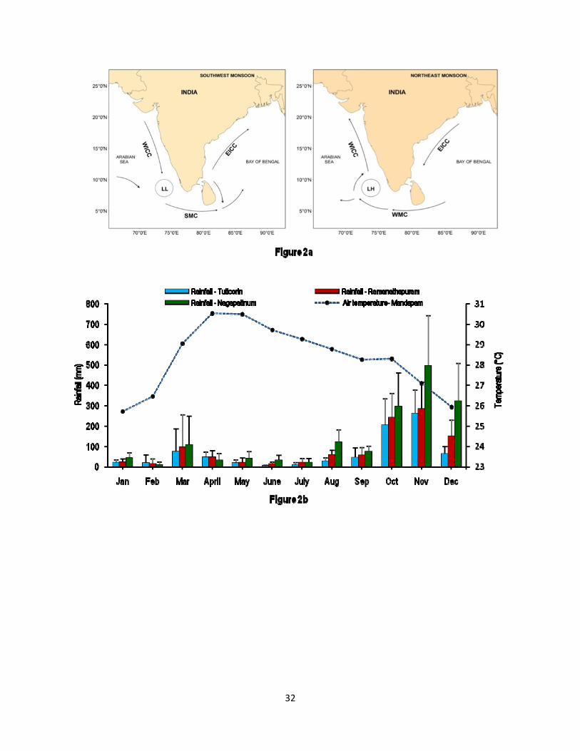
32  

33  

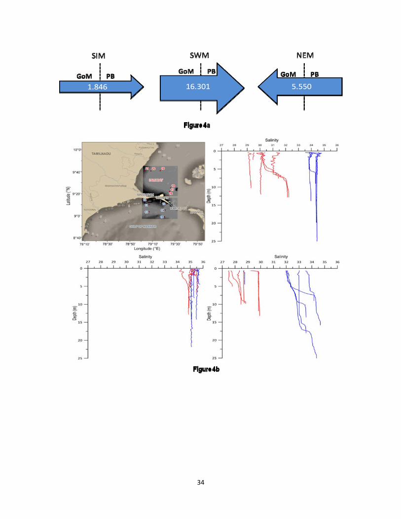
34  

35  

36  

37  

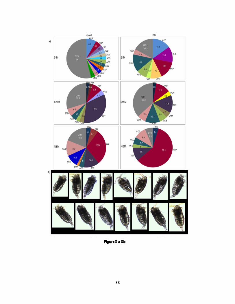
38  

39  

40  

41  

Parameters

Depth

SIM

SWM

NEM

GoM PB GoM PB GoM PB

Temperature (°C)

S 30.31 ± 1.20 31.47 ± 0.81 29.64 ± 1.11 30.29 ± 0.64 26.55 ± 0.49 25.45 ± 0.61 B 29.29 ± 0.59 30.39 ± 0.43 28.89 ± 1.48 30.24 ± 0.28 26.94 ± 0.23 25.73 ± 0.32

Salinity S 33.90 ± 0.54 30.44 ± 1.13 35.39 ± 0.60 34.90 ± 0.60 32.00 ± 0.58 28.90 ± 1.42

B 34.10 ± 0.36 31.14 ± 1.28 34.63 ± 3.30 34.38 ± 1.06 32.89 ± 1.40 29.75 ± 1.33 DO (mg L-1) S 7.81 ± 0.93 6.34 ± 0.68 7.92 ± 0.75 6.76 ± 0 .91 7.92 ± 0.75 8.12 ± 1.32

B 7.54 ± 0.69 6.66 ± 0.73 5.99 ± 1.08 6.40 ± 0.72 6.74 ± 1.18 7.64 ± 1.12 Chl.a (mg m-3) S 0.70 ± 0.45 0.87 ± 0.47 1.60 ± 1.30 0.76 ± 0.40 1.80 ± 1.70 0.75 ± 0.40

B 1.10 ± 0.60 0.56 ± 0.31 1.70 ± 1.50 1.10 ± 0.60 1.60 ± 1.40 0.74 ± 0.37 Turbidity (NTU ) S - - - - 1.76 ± 1.39 7.85 ± 13.59 B - - - - 2.73 ± 1.87 11.32 ± 18.83 APP abundance S - - 0.64 ± 0.38 1.71 ± 0.44 0.65 ± 0 .45 0.99 ± 0.40

B - - 0.42 ± 0.25 1.97 ± 1.07 0.48 ± 0.47 1.19 ± 0.47 HPP abundance S 1.28 ± 0.45 2.37 ± 0.73 0.87 ± 0 .47 0.65 ± 0.13 0.85 ± 0.22 0.65 ± 0.23

B 1.20 ± 0.50 0. 64 ± 0.12 0.83 ± 0.37 0.65 ± 0.18 0.65 ± 0.20 0.67 ± 0. 27 ANP abundance S - - 1.55 ± 0.72 0.63 ± 0.27 1.84 ± 0.90 0.77 ± 0.37

B - - 1.06 ± 0.42 0.87 ± 0.35 1.22 ± 0.83 0.59 ± 0.26 HNP abundance S 3.96 ± 0.84 6.79 ± 1.38 1.76 ± 0.64 2.60 ± 0.91 1.32 ± 0.47 2.80 ± 0.94

B 3.81 ± 0.81 6.96 ± 1.46 1.5 ± 0.32 2.34 ± 0.76 1.27 ± 0.42 2.53 ± 0.88 MZP abundance S 1757 ± 506 2968 ± 880 1020 ± 900 1362 ± 1093 940 ± 607 2389 ± 1618

B 2193 ± 584 3296 ± 1100 1213 ± 1198 1540 ± 1256 1160 ± 679 2645 ± 1429 MSP abundance S 567 ± 527 824 ± 850 580 ± 718 266 ± 344 998 ± 635 312 ± 285 Copepod abundance S 278 ± 293 631 ± 678 530 ± 729 198 ± 230 842 ± 630 316 ± 240 Phyto. biomass S 17.50 ± 11.25 21.73 ± 11.63 40.25 ± 32.5 19.00 ± 11.09 45.40 ± 44.86 18.75 ± 11.09

B 25.00 ± 27.5 14.00 ± 7.75 42.5 ± 37.5 27.50 ± 15.00 40.00 ± 35.00 18.50 ± 9.25 HPP b iomass S 14.06 ± 4.93 26.11 ± 8.11 9.62 ± 5.21 7.14 ± 1.39 9.31 ± 2.44 7.12 ± 2.58

B 13.22 ± 5.48 21.99 ± 7.27 9.10 ± 4.05 7.18 ± 1.98 7.13 ± 2.24 7.37 ± 2.95 HNP biomass S 24.37 ± 5.18 41.89 ± 8.51 10.86 ± 8.77 16.04 ± 12.77 8.14 ± 2.88 17.28 ± 2.61

B 23.51 ± 4.99 42.94 ± 9.00 9.26 ± 3.33 14.44 ± 4.69 7.84 ± 2.59 15.61 ± 5.44 MZP biomass S 25.96 ± 14.14 33.06 ± 19.23 10.46 ± 11.63 13.11 ± 11.63 9.68 ± 9.17 27.79 ± 21.07

B 29.08 ± 12.67 35.37 ± 13.97 13.04 ± 11.08 15.87 ± 14.69 12.67 ± 11.36 29.02 ± 24.55 MSP biomass S 2.30 ± 2.09 3.83 ± 3.53 4.85 ± 5.85 1.79 ± 1.52 6.63 ± 3.83 5.10 ± 4.06

Table 1 - Seasonal variations of environmental and biological parameters. Abbreviations: APP- Autotrophic picoplankton (x 107 No. L-1); HPP- heterotrophic picoplankton (x109 No. L-1); ANP- Autotrophic nanoplankton (x106 No. L-1), HNAN - Heterotrophic nanoplankton (x 106

No. L-1), MZP - Microzooplankton (No. L-1), MSP – Mesozooplankton (No. m-3) and copepod (No. m-3) are presented. All biomass values are in mg C m-3. (S) Surface waters and (B) bottom waters. Minus sign indicate absence.

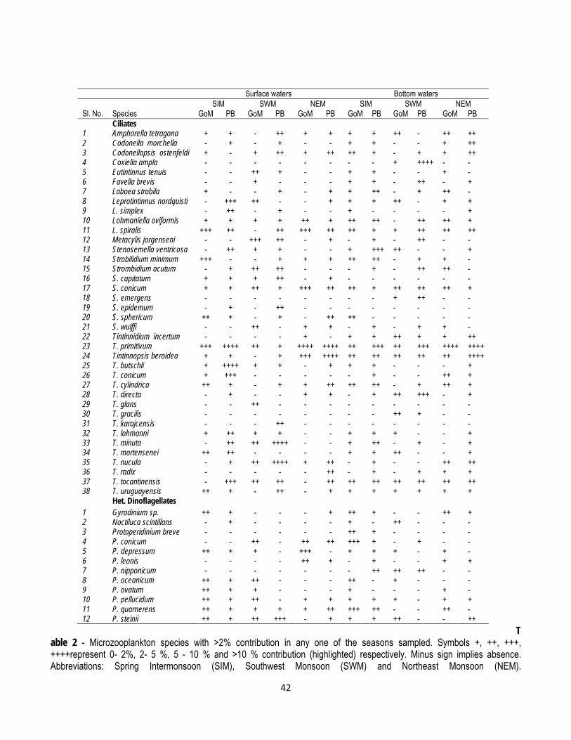
42  

Surface waters Bottom waters SIM SWM NEM SIM SWM NEM Sl. No. Species GoM PB GoM PB GoM PB GoM PB GoM PB GoM PB Ciliates 1 Amphorella tetragona + + - ++ + + + + ++ - ++ ++ 2 Codonella morchella - + - + - - + + - - + ++ 3 Codonellopsis ostenfeldi + - + ++ + ++ ++ + - + + ++ 4 Coxiella ampla - - - - - - - - + ++++ - - 5 Eutintinnus tenuis - - ++ + - - + + - - + - 6 Favella brevis - - + - - - + + - ++ - + 7 Laboea strobila + - - + - + + ++ - + ++ - 8 Leprotintinnus nordquisti - +++ ++ - - + + + ++ - + + 9 L. simplex - ++ - + - - + - - - - + 10 Lohmaniella oviformis + + + + ++ + ++ ++ - ++ ++ + 11 L. spiralis +++ ++ - ++ +++ ++ ++ + + ++ ++ ++ 12 Metacylis jorgenseni - - +++ ++ - + - + - ++ - - 13 Stenosemella ventricosa - ++ + + - - + +++ ++ - - + 14 Strobilidium minimum +++ - - + + + ++ ++ - + + - 15 Strombidium acutum - + ++ ++ - - - + - ++ ++ - 16 S. capitatum + + + ++ - + - - - - - - 17 S. conicum + + ++ + +++ ++ ++ + ++ ++ ++ + 18 S. emergens - - - - - - - - + ++ - - 19 S. epidemum - + - ++ - - - - - - - - 20 S. sphericum ++ + - + - ++ ++ - - - - - 21 S. wulffi - - ++ - + + - + - + + - 22 Tintinnidium incertum - - - - + - + + ++ + + ++ 23 T. primitivum +++ ++++ ++ + ++++ ++++ ++ +++ ++ +++ ++++ ++++ 24 Tintinnopsis beroidea + + - + +++ ++++ ++ ++ ++ ++ ++ ++++ 25 T. butschli + ++++ + + - + + + - - - + 26 T. conicum + +++ - - - - - + - - ++ + 27 T. cylindrica ++ + - + + ++ ++ ++ - + ++ + 28 T. directa - + - - + + - + ++ +++ - + 29 T. glans - - ++ - - - - - - - - - 30 T. gracilis - - - - - - - - ++ + - - 31 T. karajcensis - - - ++ - - - - - - - - 32 T. lohmanni + ++ + + - - + + + - - + 33 T. minuta - ++ ++ ++++ - - + ++ - + - + 34 T. mortensenei ++ ++ - - - - + + ++ - - + 35 T. nucula - + ++ ++++ + ++ - + - - ++ ++ 36 T. radix - - - - - ++ - + - + + + 37 T. tocantinensis - +++ ++ ++ - ++ ++ ++ ++ ++ ++ ++ 38 T. uruguayensis ++ + - ++ - + + + + + + + Het. Dinoflagellates

1 Gyrodinium sp. ++ + - - - + ++ + - - ++ + 2 Noctiluca scintillans - + - - - - + - ++ - - - 3 Protoperidinium breve - - - - - - ++ + - - - - 4 P. conicum - - ++ - ++ ++ +++ + - + - - 5 P. depressum ++ + + - +++ - + + + - + - 6 P. leonis - - - - ++ + - + - - + + 7 P. nipponicum - - - - - - - ++ ++ ++ - - 8 P. oceanicum ++ + ++ - - - ++ - + - - - 9 P. ovatum ++ + + - - - + - - - + - 10 P. pellucidum ++ + ++ - + + + + + - + + 11 P. quarnerens ++ + + + + ++ +++ ++ - - ++ - 12 P. steinii ++ + ++ +++ - + + + ++ - - ++

  Table 2 - Microzooplankton species with >2% contribution in any one of the seasons sampled. Symbols +, ++, +++, ++++represent 0- 2%, 2- 5 %, 5 - 10 % and >10 % contribution (highlighted) respectively. Minus sign implies absence. Abbreviations: Spring Intermonsoon (SIM), Southwest Monsoon (SWM) and Northeast Monsoon (NEM).

43  

Sl.No Species Occurrence Feeding habit

(GoM)

1 Acartia erythraea SIM, SWM, NEM Omn3 2 A. danae SIM, SWM+, NEM Omn4

3 A. spinicauda SIM Omn3

4 Acrocalanus gracilis SIM + Her3, Omn8 5 Calanopia minor SIM, SWM, NEM Car3

6 Centropages furcatus SIM, SWM Omn 3,4

7 C. calaninus SWM, NEM Omn3 8 C. dorsispinatus SIM, NEM Omn3 9 Corycaeus danae SIM, SWM +, NEM ++ Car3,4

10 C. speciosus SIM Car3,4

11 Eucalanus elongatus SIM & NEM Her3,4 12 Euterpina acutifrons SIM, SWM, NEM Her 3,Omn5 13 Farranula gibbula SIM, SWM, NEM Car3

14 Labidocera acuta SIM, SWM, NEM Car3,4

15 L. pava SIM Car3,

16 L. pectinata SIM & SWM Car3,

17 Microsetella sp SIM, SWM, NEM Her3

18 Oithona nana SIM, NEM Omn3,5 19 O. similis SIM, NEM Omn3,5 20 Oncaea conifera SIM, SWM Car3,Omn7 21 O. media SIM, SWM Omn7 22 O. venusta SIM, SWM, NEM ++ Car 3,Omn1,2,7 23 Onychocorycaeus catus SIM, SWM Car3

24 Paracalanus parvus SIM, SWM +, NEM # Her 4, Omn5 25 Pareucalanus attenuatus SIM, SWM, NEM + Her3,4

26 Pseudodiaptomus serricaudatus SWM Omn3

27 Subeucalanus crassus SIM Her3

28 Temora discaudata SIM, SWM Omn3

29 T. stylifera SIM, SWM Omn5 30 T. turbinata SIM, SWM #, NEM ++ Omn3,5, Her4

31 Tortanus barbatus SIM, SWM, NEM Car3

32 Undinula vulgaris SIM, SWM, NEM Omn6

(PB) 1 Acartia erythraea SIM +, SWM + , NEM Omn3 2 A. danae SIM ++, SWM ++, NEM + Omn4 3 A. spinicauda SIM Omn3 4 Acrocalanus gracilis SIM ++, SWM, NEM Her3, Omn8 5 Calanopia minor SIM, SWM Car3 6 Centropages furcatus SIM Omn 3,4 7 C. orsinii SIM +, NEM Omn4

8 Clausocalanus arcuicornis SIM ++, SWM, NEM Her3,4 , Omn5 9 Corycaeus danae SIM, SWM +, NEM + Car3,4, 10 Euterpina acutifrons SIM & NEM Her3 , Omn5 11 Oithona similis SWM Omn3,5 12 Paracalanus parvus SIM ++, SWM ++, NEM ## Her 3,Omn5 13 Pseudodiaptomus aurivilli SWM Omn3

14 P. serricaudatus SWM Omn3 15 Temora turbinata SIM, SWM ++, NEM ++ Omn3,5,Her4 16 Undinula vulgaris SWM, NEM Omn6

Table 3 – Copepods abundance and their feeding behavior. Abbreviations: Spring Inter-monsoon (SIM), Southwest Monsoon (SWM) and Northeast Monsoon (NEM). Symbols: + indicates >5 - 10 contribution, ++ indicates >10-20 % contribution; # indicates 20-40 % contribution; ## indicates 40-60 % contribution. 1Fernandes and Ramaiah, 2009., 2Kattner et al, 2003., 3Rakesh et al, 2008., 4Richardson et al., 2006, 5Broglio et al, 2004., 6Goswami and Padmavati, 1996., 7Ohtuska et al, 1996., 8Mc Kinnon and Ayukai.,1996.