No. 11-10

Trends in U.S. Family Income Mobility, 1969–2006 Katharine Bradbury

Abstract: Much of America’s promise is predicated on economic mobility—the idea that people are not limited or defined by where they start, but can move up the economic ladder based on their efforts and accomplishments. Family income mobility—changes in individual families’ income positions over time—is one indicator of the degree to which the eventual economic wellbeing of any family is tethered to its starting point. In the United States, family income inequality has risen from year to year since the mid-1970s; given this rising cross-sectional inequality, changes over time in mobility determine the degree to which long-term income is also increasingly unequally distributed.

Using data from the Panel Study of Income Dynamics and a number of mobility concepts and measures drawn from the literature, this paper examines family income mobility levels and trends for U.S. working-age family heads and spouses during the time span 1969–2006, based on a post-tax, post-transfer concept of income adjusted for family size. By most measures, mobility is lower in more recent periods (1995–2005) than in the late seventies and the eighties (the 1977–1987 or 1981–1991 periods). Comparing results based on pre-government income suggests that an increasingly redistributive tax and transfer system contributed to rising mobility into the 1980s, but that its impact has since waned. Overall, the evidence indicates that over the 1969-to-2006 time span, family income mobility across the distribution decreased, families’ later-year incomes increasingly depended on their starting place, and the distribution of families’ lifetime incomes became less equal.

JEL codes: D31, D63, I32, J15 Keywords: Income mobility, income inequality, income distribution Katharine Bradbury is a senior economist and policy advisor at the Federal Reserve Bank of Boston. Her e-mail address is katharine.bradbury@bos.frb.org.

This paper presents preliminary analysis and results intended to stimulate discussion and critical comment. The views expressed herein are those of the author and do not indicate concurrence by other members of the research staff or principals of the Federal Reserve Bank of Boston or the Federal Reserve System.

This paper, which may be revised, is available on the web site of the Federal Reserve Bank of Boston at http://www.bos.frb.org/economic/wp/index.htm.

This paper builds heavily on earlier joint work with Jane Katz, Officer and Director of Education Programs at the Federal Reserve Bank of New York; while she is not co-author, her insights added immeasurably to the research. Peter Gottschalk generously provided edited data files from the Panel Study of Income Dynamics, without which this analysis would have been much more difficult to complete; Dean Lillard helped me understand the CNEF files at Cornell University. I am also grateful to Mary Burke, Jane Little, Bob Triest, Dan Aaronson, two anonymous referees, participants at the May 2009 conference of the System Committee on Applied Microeconomics and at the November 2009 APPAM meetings for helpful comments on earlier drafts, to participants in a Boston Fed departmental seminar for comments on a very early presentation of this work, and to Jessamyn Fleming, Charu Gupta, and Ryan Kessler for outstanding research assistance and comments. I am responsible for any remaining errors.

This version: October 20, 2011

1

Much of America’s promise is predicated on the existence of economic mobility—the

idea that people are not limited or defined by their current circumstances, but can move up the

income ladder based on their effort and accomplishments. Can a poor individual or family rise

into the middle class, or is longer-term economic status limited by one’s economic situation at a

given point in time?

Changes in economic mobility are of particular consequence when economic disparities

among families are increasing over time, as has been the case in the United States in recent

decades. If family income inequality is increasing, changes in the degree to which families move

up and down can either offset or amplify longer-term inequality—and loosen or tighten the link

between a family’s circumstances in any given year and its later outcomes. Other things being

equal, an economy with rising mobility—one in which families move increasingly frequently or

traverse increasingly greater distances up and down the income ladder—will result in a more

equal distribution of lifetime incomes than an economy with declining mobility.

This paper examines time patterns of family income mobility for U.S. working-age

family heads and spouses between 1969 and 2006, using data from the Panel Study of Income

Dynamics (PSID) and a number of mobility concepts and measures, including a measure of the

degree to which mobility equalizes long-term incomes. Calculating these measures for

overlapping 10-year periods, the paper documents mobility levels and trends based on pre- and

post-government measures of family income adjusted for family size.

By and large, different mobility measures and income measures yield similar pictures of

mobility trends. Most mobility measures indicate that family income mobility was lower in

more recent periods (the 1990s into the early 2000s) than in earlier periods. Comparing 1977–

1987 or 1981–1991, when many of the measures peaked, with the most recent period (1995–

2005), mobility declined to a statistically significant degree according to most measures, both

overall and for individuals beginning near the top or bottom of the income distribution.

However, comparing periods ending in the most recent 10 or so years (1985–1995 through 1995–

2005), depending on the mobility measure employed, trends are difficult to discern, except that

mobility was lower in the last period (1995–2005 or 1996–2006) than in the period immediately

2

before (1993–2003 or 1994–2004). Comparing these post-government trends with results based

on pre-government income suggests that the redistributive impact of the U.S. tax and transfer

system may have contributed more positively to mobility in the 1970s than it has since 1981.

As the opening paragraphs above indicate, a key reason for studying mobility trends is a

concern with lifetime income inequality. Although the calculations reported here track

individuals over 10 years (far less than a lifetime), the distribution of long-term income (family

income averaged over 10 years, or even 16 years) was much more unequal in recent periods

than in the 1970s. The trend has been visibly steep, regardless of the inequality measure or

income measure employed. Thus, whether the declines in measured mobility are significantly

different from zero or not, mobility levels and trends have not been sufficient to offset the

considerable rise in short-term inequality.

The paper proceeds as follows: The first section below provides an overview of existing

literature related to changes over time in family income mobility. The following section

discusses concepts of income mobility and outlines the concepts and measures used in this

paper (an appendix provides actual definitions of the measures). The next section describes the

data and sample used in the analysis: the “base case” measure of income, how it is adjusted for

family size, and the mobility “periods” examined. Three sections follow that report and discuss

results according to various mobility measures and examine their time trends. The next two

sections introduce comparisons of the post-government base case with the pre-government

income case, looking at “mobility” for individuals from their pre-government income status to

their post-government income status within a year and at mobility measured over 10-year

periods based on pre-government income. The final section summarizes and discusses the

results.

Literature Review

An extensive literature explores the extent of economic mobility in the United States and

other nations. Much of that research focuses on earnings mobility, examining how individuals’

earnings change over time. Another set of papers focuses on family income mobility, measuring

the degree to which individuals’ family incomes change from one point in time to another, and

3

a subset of that research investigates how family income mobility patterns have changed over

time. The current paper contributes to this latter literature, measuring U.S. family income

mobility with a variety of measures and in many overlapping time periods in order to explore

their time patterns: It asks whether U.S. family heads and spouses were more or less likely to

move up and down the family income ladder in recent periods than in earlier decades,

comparing, for example, mobility during the 1996–2006 period (most recent available) with that

during 1969–1979 (earliest available) or with some other 10-year period in the middle of the

1969–2006 span. And it explores whether the answer to this question depends on the specific

measures of mobility or of family income or on a focus on specific parts of the income

distribution.

At least 10 research papers examine U.S. family mobility in two adjacent “long” periods

(mostly decades), focusing largely on relative (quintile- or decile-based) mobility measures.1

1 Fields and Ok (1999) compare the early part of two decades, but use only absolute measures—income flux and directional income change—based on individual changes in log income (which they describe as “a particular facet of the multi-faceted notion of income mobility,” p. 467). They say their finding of a statistically significant increase in (family) income flux in the United States between the 1969–1976 and 1979–1986 periods is complementary to “earlier findings of others who demonstrated that relative mobility in the United States has been unchanged or falling over the same period of time” (p. 457).

Using data from the Panel Study of Income Dynamics, Acs and Zimmerman (2008a) report “no

change” in family income mobility between 1984–1994 and 1994–2004, although the reported

values of their quintile-based mobility measures decreased somewhat between the two decades.

Based on tax returns, Auten and Gee (2009) find the “degree of relative income mobility among

income groups” is very similar in 1987–1996 and 1996–2005, although mobility out of the top

quintile declined somewhat between the two periods. Hungerford (2008, 2011) compares the

1980s and the 1990s and finds that “relative income mobility was lower in the 1990s than in the

1980s” (2008, p. 9) and, more specifically, that “reranking or positional income mobility

decreased from the 1980s to the 1990s” (2011, p. 96). Bradbury and Katz (2002) see a slight

decline in mobility between the 1980s and the 1990s, following no change between the 1970s

and 1980s. Carroll, Joulfaian, and Rider (2006) find that relative mobility declined somewhat

between 1979–1986 and 1987–1995.

4

Looking at even earlier periods, Sawhill and Condon (1992), Hungerford (1993), and

Gittleman and Joyce (1999) report little change in overall family income mobility between the

1970s and the 1980s. The latter two studies, however, find “subtle differences” (Hungerford’s

term), suggesting that some groups were less upwardly mobile in the later decade. Focusing on

young children, Gottschalk and Danziger (2001) also find little difference in family income

mobility between the 1970s and the 1980s, although children whose families began with low

income (poorest two quintiles) or high income (richest quintile) were somewhat less mobile in

the later period.

The results in this paper are broadly consistent with this literature, and the “Results”

and “Time Trends” sections below provide more detailed comparisons. The paper reports a

variety of measures on a consistent basis for overlapping 10-year time periods over a 37-year

time span and is able to compare and contrast the trends in the literature with those observed

here. Thus, this paper contributes to the literature by examining mobility over a considerably

longer time span and investigating a broader range of mobility measures, and it offers a new

categorization of mobility measures as well as comparisons of mobility based on pre- and post-

government incomes.

Mobility Concepts and Measures

In broad terms, mobility is the pace and degree to which individuals’ or families’

incomes (or other measures of wellbeing) change over time relative to one another or relative to

the overall income distribution. Some researchers define mobility even more broadly to

encompass movements that have no “relative” aspect, such as the average change in (log)

incomes or the average absolute value of (log) income change. While overall income growth

obviously contributes to average wellbeing, this paper treats it as a feature of income change

that is distinct from mobility. Thus, the mobility measures examined in this paper all have a

relative aspect, comparing families’ income changes with one another, not simply computing

average changes.2

2 Fields (2008a) notes that a “difference of view—whether ‘income mobility’ includes the growth aspect of distributional change or whether ‘mobility’ is what remains after growth has been taken out—underlies

5

Among concepts and measures with a relative aspect, this paper emphasizes the features

that help to address the questions posed at the outset: How limited is a person by his/her

current circumstances and how are income changes contributing (or not) to the inequality of

lifetime incomes?3

The paper uses a variety of relative measures in order to understand whether they all

tell a consistent story and whether findings from previous studies are artifacts of particular

measures. Reflecting an interest in mobility during a working life, the paper examines mobility

over the long term (10-year periods); it does not address shorter-term “volatility”—shocks to

family incomes from year to year—nor even longer-term intergenerational mobility—how

much a person’s prime-age family income level (or position) depends on the corresponding

level (position) of his/her parents during his/her childhood.

The degree to which end-of-period income (or position) is independent of

beginning-of-period income or position is related to the idea of equal opportunity. In their

“introduction to the literature” on income mobility measurement, Fields and Ok (2001) note that

“origin independence seems to capture our intuitions about ‘equality of opportunity’… Viewed

in this way, income mobility is a desirable notion that helps attenuate the unequal distribution

of initial endowments.” (p. 561). Mobility as an equalizer of longer-term or lifetime incomes, by

contrast, associates more equal long-term outcomes (not opportunities) with improved

mobility.

The sections that follow discuss two ways of categorizing mobility concepts. When

cross-classified, the two category types yield the two-by-two matrix shown in Table 1, which

lists the specific measures from the literature used in this paper; the appendix defines the

measures.

much of the mobility literature, but rarely is made explicit.” For this reason, I am being explicit that the definition used in this paper excludes that pure average-growth aspect. Van Kerm (2002) explicates the distinction as follows: he says the Fields and Ok (1999) flux concept of mobility, depending as it does on absolute change in log income, "differs from most approaches to income mobility measurement in one important respect: income mobility is seen as the juxtaposition of isolated individual experiences and not as an intrinsically social phenomenon where it is individual experiences relative to the experiences of others that matter." (p. 232, emphasis added). In these terms, the mobility investigated in this paper, like “most approaches,” is a social phenomenon. 3 “Lifetime” income typically refers to a person’s average income over a number of years; the current analysis focuses on average income in a 10-year period during the working-age years.

6

Position-relative and dollar-relative mobility

One categorization is built around the specific aspects of income movement considered;

these define the two horizontal panels in Table 1.

Position-relative mobility (upper panel) refers to individuals moving among positions in

the distribution of family incomes between the beginning and end of a period, where positions

are defined in a purely relative way. Position-relative measures are typically based on transition

matrices showing position in terms of quintile, decile, or other quantile at the beginning and the

end of a period, but they can also be expressed more granularly in terms of rank. What makes

them position-relative is that they do not reflect the dollar size of incomes or the spread of the

income distribution, but only rank.

Dollar-relative mobility (lower panel) refers to changes in individuals’ family incomes and

associated changes in their relative positions. This concept encompasses income movement both

relative to some real standard of wellbeing or purchasing power and relative to the (possibly

changing) overall distribution of income. Dollar-relative mobility can reflect changes in the

structure of rewards in the economy—the addition, for example, of much higher places at the

top of the distribution—as well as changes in individuals’ access to these rewards.

Dollar-relative measures are useful for summarizing how much movement the average

family experiences—both relative to other families and in terms of absolute (dollar) income

change—taking into account changes in average income levels and the inequality of the income

distribution. Some of these measures directly indicate the degree to which longer-term incomes

are equalized by income movements in a period; others shed light on the degree to which an

individual’s initial family income position persists.

Overall and origin-specific mobility

The second categorization is based on the individuals for whom family income

movements are considered—part or all of the initial distribution; these define the two vertical

panels in Table 1.

Overall mobility (left-hand column) summarizes the transition process from the economy-

wide set of individual observations of wellbeing—whether income or rank—at the start of a

7

period to the corresponding set at the end of that period. Overall mobility measures attempt to

quantify the extent to which the entire economy is characterized by families with persistent

positions versus families experiencing widespread movement. They also may summarize the

economy-wide association between families’ changes in rank and absolute income or the degree

to which families’ patterns of movement are making longer-term incomes more or less equal.

Origin-specific mobility (right-hand column) summarizes movements of subgroups

defined by their position (rank, income) in the distribution at the beginning of the period.

Origin-specific mobility measures attempt to quantify the extent to which those who start at the

bottom/top (or, more generally, in any specific part of the distribution) move up/down either

relatively (rank, position) or absolutely (by crossing some real dollar threshold) by the end of

the period.

Origin-specific measures are of interest for several reasons, including concerns about the

ability of the poor to escape the bottom rungs of the income ladder and concerns about stability

at the top, as evidence of unequal opportunity or a lack of meritocracy. Along these lines,

Burkhauser and Couch (2009) note that studies of origin-specific mobility “have been motivated

by an interest in whether those at the top and bottom of society are differentially mobile but

also by an interest in the degree to which spells in poverty impact future movement up the

income distribution.” (p. 523). In this regard, a recent Pew Trusts survey found that "a majority

of Americans believe that the lack of upward mobility from the bottom rung of the income

ladder is a major problem for this country, while they are relatively unconcerned about how

little downward mobility there is from the top” (Economic Mobility Project 2009, p. 4).

Data and Sample

The mobility measures discussed above and defined in the appendix are calculated

using data from the Panel Study of Income Dynamics (PSID), which has collected information

on the incomes and characteristics of individuals and their families since 1968. The survey was

conducted every year from 1968 through 1997 and every other year thereafter; the most recent

survey for which income data are available, conducted in 2007, provides data on incomes in

2006.

8

Each period’s measures include all individuals who meet the following criteria at both

the beginning and end of the period (or throughout the period for measures that use all years):

• individual is a family head or spouse

• both the family’s head and spouse (if present) are between 16 and 62 years old4

• family income data are not missing.

In addition, at the beginning of a period, the individual’s family may not be a “split-off,”

meaning that the family must have been separate from the head’s parents’ family for at least a

year.5 Thus, the sample (approximately 2,500 to 4,000 observations) changes for each period.

The observations are weighted using individual weights, to correct for the PSID’s over-

sampling of the bottom of the income distribution.6

The paper examines two measures of family income. One is pre-government family

income, which comprises pretax, pre-transfer money income of all family members combined,

including wages, salaries, rent, interest, dividends, farm and business income, pensions,

alimony, child support, and help from relatives and others. The second income measure is post-

government family income, which subtracts net income taxes (“net” meaning that it also reflects

the potentially positive addition of the earned income tax credit for low-income families with at

least one worker) and adds in the cash value of food stamps along with social security benefits

and all government cash transfers, such as welfare. The pre-government and post-government

measures are drawn from Cornell University’s Cross-National Equivalent File for the PSID.

7

4 For mobility measures based on two-year average endpoints (the base case in Figures 1 through 4), heads and spouses are between 16 and 62 years old in both years used in computing both endpoints. Thus, for example, the measures shown in Figure 1 for the 1995–2005 period are based on heads and spouses who are 16 to 62 years of age in 1994, 1996, 2004, and 2006; hence they are 16 to 50 years of age in 1994 and 28 to 62 years old in 2006.

Income and other dollar-based measures are adjusted for inflation using the CPI-U-RS.

5 Since income is reported for the calendar year prior to the survey, split-off families’ reported income includes the full- or part-year income of the parental family. The exclusion of split-off families thus insures that measured mobility reflects the individual’s independent family income changes, not the income movements that result when children move from parental to independent family income. 6 After exclusion of observations with zero weight in either year, the individual weight is averaged over all the years included in each period’s measure. 7 Cornell University imputes net taxes via the TAXSIM model, and assumes that all taxpaying units take the standard deduction and all eligible families file for the earned income tax credit.

9

For post-government income, the observations in the highest and lowest (weighted)

percentile of each year’s head-and-spouse distribution are trimmed out. This eliminates any

top-coded and bottom-coded observations as well as the most extreme measurement errors.

Only the highest 1 percent are trimmed from the pre-government income measure because it is

impossible to trim the poorest percentile without trimming more than 1 percent, and because

the income values at the bottom have a reasonable interpretation. From 1½ to 5 percent

(depending on year) of weighted heads and spouses have zero pre-government income,

indicating that the family has no income in the absence of government transfers or social

security.8

Family income is adjusted for family composition to yield a more accurate indicator of

wellbeing; for example, $45,000 represents a very different standard of living for a family of five

than for a two-person family. The adjustment divides family income by the square root of

family size, an equivalence scale used in a number of research papers.

The zeros therefore do not represent extreme values or likely measurement error, and

dropping all of them would leave a biased sample of pre-government incomes. When

comparing measures based on pre- and post-government income, the measures incorporate

only observations present in both samples.

9

In most of the analysis that follows, the reported measures relate to a “base case,” in

which the following holds:

• The measure of income is post-government income adjusted for family composition

using the square root of family size;

8 After 1996, some observations have negative pre-government income; these are set to zero for consistency with the data for 1969 through 1996 (when the PSID set all negative income values to zero or $1). 9 Burkhauser et al. (1996) explore the implications of using several possible equivalence scales in measuring inequality, including the poverty line and some based on expenditures; they label the square root of family size the “International Experts” scale. Karoly and Burtless (1995) adopt the square root of family size in their exploration of Gini inequality and report only modest differences in the trend from using 0 (no adjustment of total family income) vs. 0.5 (their Appendix Table 1). Burkhauser, Larrimore, and Simon (2011) say that dividing by the square root of the income-sharing-unit’s size is “the customary procedure in the income inequality literature” (p. 13). The most widely used alternatives are to adjust family income by dividing by the Census poverty line, which varies with family size (and, over time, with inflation), or by dividing by the PSID “needs” measure, a similar scale based on the USDA “low cost” food standard.

10

• The period for measuring mobility is 10 years: and

• Adjusted income is averaged for two years at both the start and the end of the 10-

year period.

Averaging two years of adjusted income at the period endpoints is intended to smooth some of

the transitory income changes that occur on a year-to-year basis as well as reduce the effects of

measurement error in single-year income. Because the data are collected only every other year

after the 1996 income year (1997 survey), the two-year endpoints are calculated by averaging

non-adjacent years (t-1 and t+1); for consistency, this approach is also used before 1996. Labels

refer to year t; thus, for example, “2005” is the average of 2004 and 2006 income data, so the

period 1995–2005 reflects income changes between the average of 1994 and 1996 and the

average of 2004 and 2006.

One set of measures—Shorrocks M and the inequality of long-term incomes on which it

is based—is computed using the average of all the observations on each individual’s adjusted

family income within a 10-year period rather than just the beginning and end years. Because

data are available only every other year, the average includes income over the six years

comprising every other year within each 10-year period (the computations are the same—

averaging every other year—even in the earlier periods during which data exist for all years).

For example, the most recent 10-year average measure, for 1996–2006, averages family income

for each head or spouse observed in 1996, 1998, 2000, 2002, 2004, and 2006.

Results for Position-Relative Mobility

Position-relative mobility measures consider families’ movements in relative position

from the beginning to the end of a period, where relative position is indicated by quintile,

decile, or some other rank-based indicator. As noted earlier (and as categorized in Table 1),

position-relative mobility can be measured for all individuals combined (overall) or for subsets

defined by where in the distribution they begin the period (origin-specific).

Overall position-relative mobility

Figure 1 displays five position-relative overall mobility measures for the base case and

11

Table 2 reports the values.10

Auten and Gee’s (2009) tax-return-based mobility matrices indicate a slight decline in M-

hat (from 0.702 to 0.695) between 1987–1996 and 1996–2005;

The time patterns of the individual measures are very similar: most

of them increase somewhat or move sideways between 1970–1980 and 1977–1987 or

thereabouts, decline non-monotonically through 1989–1999, level out or rise slightly, and

decline again between 1991–2001 or 1993–2003 and 1995–2005. They all indicate less family

income mobility for U.S. individuals in the (most recent) 1995–2005 period than in the 1970s. For

example, 78 percent of individuals moved up or down one decile or more in the first few

periods, while 75 to 76 percent changed deciles during the last few periods. The number of

deciles the average person moved declined from 1.9 to 1.7. M-hat decreased from around 0.76 to

0.72, and the correlation of an individual’s beginning-of-period and end-of-period income rank

rose from 0.62 to 0.65, indicating mobility (as measured by the inverse rank correlation)

declined. The inverse adjusted contingency coefficient C* fell from 0.36 to 0.33. While these are

all small changes, they are consistently negative across the position-relative overall measures.

11 our data also show declines in

these measures between 1987–1997 and 1995–2005.12 The quintile mobility matrices reported in

Tables 7–9 of Carroll, Joulfaian, and Rider (2006) indicate that M-hat fell slightly (from 0.70 to

0.68) between the 1979–1986 and 1987–1995 periods; over this time span, Table 2 below shows

declines in M-hat (for 10-year mobility) as well. For even earlier decades, Gittleman and Joyce

(1999) document a gradual increase in mobility between 1967–1977 and 1981–1991; they display

(graphically) the quintile immobility ratio (fraction staying in origin quintile), which moves

from about 0.37 for 1967–1977 to 0.355 in 1981–1991; they also report a slight increase in

mobility between two adjacent 12-year periods, 1967–1979 and 1979–1991.13

10 Two of the measures have been re-scaled in the figure so that all of them can be displayed together.

As noted above,

Table 2 and Figure 1 below also show increases in mobility across 10-year periods through the

11 Their National Tax Journal paper does not include mobility matrices defined over the panel population for both periods, but their working paper (2007) does (Appendix Table A.5). 12 In the “time trends” section below, I compare my results with those of Acs and Zimmerman (2008) and other researchers who use adjacent decade pairs. 13 Gittleman and Joyce use PSID income adjusted by the poverty line and follow individual heads and spouses ages 25 to 64. The immobility ratio figures are based on their smoothed (“predicted”) series in the lower panel of Figure 1; their Table 5 reports quintile mobility matrices for 1967–1979 and 1979–1991.

12

end of the 1980s. Data from Gottschalk and Danziger (2001) and from Sawhill and Condon

(1992) show no change in M-hat between the 1970s and the 1980s.14

Origin-specific position-relative mobility

Similarly, Hungerford

(1993) reports no change in mobility between the 1970s and 1980s (in his case, the comparison is

between the 1969–1976 and 1979–1986 periods), although his decile mobility ratio declines from

77.0 to 75.6.

Origin-specific mobility measures focus on the movement of those who begin in a

specific segment of the initial distribution. Figure 2 shows the percentages falling out of the top

quintile and rising from the bottom quintile, respectively, and also the percentages of those who

start in the richest or poorest quintile and move “far” relative to the distribution, defined as

beyond the adjacent quintile; the right-hand panel of Table 2 reports the measures. The first

thing to note in Figure 2 is that those who begin in the poorest quintile are less likely to move

up than those who begin in the richest quintile are to move down; this lower mobility of the

poor applies both to any movement out of origin quintile and to far moves.

Regarding time patterns, like the overall position-relative measures, these origin-specific

measures rise slightly or move sideways initially, decline gradually until 1987–1997 (poor) or

1989–1999 (rich), rise a bit, and then fall again between 1993–2003 and 1995–2005. The decline in

mobility is somewhat more pronounced for those who begin rich than for those who start a

period in the poorest quintile, but not so for bigger moves.

Auten and Gee’s (2007) tax-return-based mobility matrices show decreases in the

percentage of the richest quintile who move down (from 41.6 to 39.6) and who move far (from

18.1 to 16.5) between 1987–1996 and 1996–2005; Table 2 below also shows declines when

comparing 1987–1997 and 1995–2005. For earlier periods, Hungerford (1993) reports his data in

terms of decile transition matrices, but when combined into quintiles his data show 43.6 percent

of the poorest quintile moving up between 1969 and 1976, and 42.4 percent moving up between

14 For Gottschalk and Danziger, M-hat calculated with their quintile mobility matrices (Table 5.1) is 0.701 in 1971–1981 and 0.698 in 1981–1991; their measures use three-year average endpoints. For Sawhill and Condon, M-hat calculated for their quintile mobility matrices (Table 1) is 0.756 for 1967–1976 and 0.759 for 1977–1986.

13

1979 and 1986. Gottschalk and Danziger (2001) report slight declines in the fraction of children

starting in the poorest or richest quintiles who move out between the 1971–1981 and 1981–1991

periods, and more noticeable declines for “far” moves by initially poorest-quintile children

(falling from 14.8 to 12.4 percent) and for children starting in the richest quintile (from 18.5 to

11.3 percent). By contrast, Sawhill and Condon (1992) see higher fractions moving out of the

bottom and top quintiles in 1977–1986 than in 1967–1976. Indeed, across the early periods,

Figure 2 and Table 2 below also fail to show declines in origin-specific relative mobility.

Results for Dollar-Relative Mobility

Overall dollar-relative mobility, part 1

Figure 3 displays three measures of dollar-relative overall mobility for the base case

(also see Table 3). The Gini mobility measure, which reflects the association of changes in rank

and income during a period, exhibits a time pattern similar to those of the overall position-

relative (that is, rank-based) measures in Figure 1, moving generally downward after being

level across the first several periods.

The other two measures declined markedly between 1970–1980 and 1980–1990, rose

gradually from 1980–1990 to 1991–2001 or 1993–2003, and then fell again to the last (1995–2005)

period. The elasticity of end-year income with respect to beginning-year income rose from

around 0.65 in the first few periods to 0.75 in the last, indicating a decline in mobility in terms of

the degree to which end-year income moves independently of beginning-year income. The

Fields directional mobility-as-equalizer measure also fell15,16

Figure 4 displays absolute quintile mobility measures (also Table 3). Absolute quintile

15 Note that the Fields measure—which, being directional, can be negative—is positive but close to zero throughout the entire span, indicating that the average of family income over the beginning and end years of each period is only slightly more equal than the beginning-year measure. 16 Hungerford (2011) reports values of Fields mobility-as-equalizer measure (measured over all years, not just beginning and end—see appendix discussion), showing increases between the 1980s and 1990s; my results also show a rise between 1979–1989 and 1989–1999 (Figure 3). Hungerford also reports the Gini mobility measure as declining by a statistically significant amount (from 0.36 to 0.34) between the 1980s and 1990s, whereas my Gini mobility measure decreases by even more (from 0.38 to 0.32) between 1979–1989 and 1989–1999.

14

mobility indicates the percentage of all individuals moving out of (up or down from) their

quintile of origin defined in real dollar terms. This fraction rose somewhat from the 1970s

through the 1980s, declined slightly, and then held steady.

Origin-specific dollar-relative mobility

Figure 4 also plots measures of real dollar movements by those beginning the period in

the poorest or richest quintiles. Dollar movement out of the poorest quintile involves an

increase in real income large enough to move above the constant-dollar beginning-of-period

quintile ceiling by the end of the period (“percentage of the poorest who rise past real ceiling”).

Reflecting overall real income growth as well as relative starting position, these dollar-relative

mobility fractions are larger than the position-relative ones shown for the poorest quintile in

Figure 2. Indeed, the time pattern of the percent poor climbing above the real dollar ceiling of

their origin quintile tracks very closely the time pattern of within-period real income growth

(the line immediately below it in Figure 4);17

Earlier research investigating these absolute quintile mobility measures is mixed. Acs

the corresponding percentage of the richest

quintile falling below the real dollar floor of their origin quintile displays roughly its mirror

image. Thus, absolute mobility out of the poorest quintile rises steeply from 1972–1982 to 1982–

1992 as real income growth increases, declines slightly, and then moves more or less sideways;

the reverse is true of absolute mobility out of the richest quintile (except that the low point is

1981–1991, the peak period for real income growth). The dashed lines plot the percentages of

individuals in the poorest/richest quintiles who move far in absolute terms—beyond the real

dollar ceiling/floor of the adjacent quintile. Not surprisingly, real income growth augments

dollar-relative upward mobility for the poor and suppresses dollar-relative downward mobility

for the rich; since real income growth bears little relationship to the position-relative

movements of these same poor and rich, the time patterns of the position-relative mobility

measures differ from these dollar-relative measures.

17 The solid black line plots the average change (across all families) in the log of family income between the beginning and endpoint of the period, that is, average real income growth during the period. This is the “directional income movement” measure as defined by Fields and Ok (1999), which I do not report as a mobility measure because it has no relative aspect.

15

and Zimmerman (2008b) report a drop in overall absolute quintile mobility from 0.627 to 0.598

between 1984-94 and 1994-04 (not significantly different from zero), a near-zero increase in

mobility out of the bottom quintile and a statistically significant increase in mobility out of the

top quintile (their Table 4).18

Overall dollar-relative mobility, part 2: Shorrocks M

Hungerford (1993, combining his data for deciles into quintiles)

shows overall absolute quintile mobility falling slightly (from 60.5 to 59.5) between the 1970s

and 1980s, with absolute upward mobility from the poorest quintile falling, and absolute

downward mobility from the richest quintile increasing.

Shorrocks M compares the inequality of family income averaged over several years (the

“long term”) with the inequality of single-year family income averaged over the years included

in the long term. Shorrocks-M mobility is higher when individuals’ year-to-year movements

(reflected in the long-term average) offset a greater fraction of the inequality of single-year

incomes. Any relative mobility (families changing places in the distribution) makes the

distribution of long-term income more equal than the (average) distribution of single-year

incomes during the period; Shorrocks M quantifies the degree to which it is more equal. Long-

term income is defined as the average of all the observations on each person’s family income

within a 10-year period.19

18 Acs and Zimmerman (2008b) is the most comparable analysis of recent data in the literature; two key differences are the age range for their sample and their income definition. As I do, they use the PSID, employ two-year average endpoints, examine mobility in a 10-year period, and sample only heads and spouses (partners); the period that they call 1994–2004 uses an average of 1992 and 1994 income for the beginning of the period and averages income in 2002 and 2004 for the end (this is the period that I call 1993–2003). They base their analysis on a pre-tax, post-transfer definition of income, while I use post-government (post-tax, post-transfer) income; they limit their study to heads and partners who are between 25 and 45 years old at the beginning of the period, while my age limit of 16–62 becomes 16 to 52 in their beginning-of-period terms; hence I include people from nine years younger through seven years older than they do. They adjust for family size using the PSID-provided USDA needs measure, while I use the square root of family size.

The inequality of that long-term income is computed using three

alternative measures: the Gini coefficient, Theil entropy, and the mean log deviation (MLD).

19 As noted earlier in the text, available data limit the computation to income averaged over the six years comprising every other year within each 10-year period. However, for the periods from 1969–1979 through 1986–1996, data are available for every year, making possible a robustness check: Averaging 11 rather than six years of income yields a measure of inequality that is smoother than the every-other-year measure, but almost identical in level and time pattern.

16

Figure 5 displays Shorrocks M based on the three inequality measures (also Table 4). All

three show similar time patterns, declining until the 1981–1991 period, increasing thereafter,

and ending with higher levels of Shorrocks-M mobility than in the first few periods. The largest

increase occurs for the MLD-based measure, which indicates that mobility offset about 27

percent of short-term inequality in the first few periods and 32 percent in the last few. By

contrast, the Gini-based measure shows a lower level of mobility and very little increase.20

Although mobility has offset an increasing fraction of single-year inequality, a key

background fact is that the U.S. income distribution has displayed steep increases in single-year

or cross-sectional family income inequality in the 1980s, 1990s, and 2000s, as shown in Figure 6.

An extensive literature has documented this rise in family income inequality; for example,

Burkhauser, Feng, and Jenkins (2009) and Gottschalk and Danziger (2005) report steep increases

in family income inequality in the 1980s, with further increases, but at a slower pace, in the

1990s.

21

20 Transitory shocks are likely to show up as extreme values in a single year—hence contribute disproportionately to single-year inequality—and be wiped out by long-term averaging. The Theil and MLD measures are more sensitive to extreme income values (top and bottom, respectively) than is the Gini; as a result, they show more reduction in inequality than the Gini in moving from short-term to long-term income. Over time, the MLD-based mobility measure would rise more than the Gini if, for example, year-to-year (transitory) income changes that disappear in the long-term average, especially at the bottom of the distribution, accounted for an increasing fraction of (rising) single-year inequality. Hungerford (2011) reports an increase in the Gini-based Shorrocks-M mobility (long-term equalization) measure, from 0.109 in the 1980s to 0.111 in the 1990s; mine rises from 0.126 to 0.131 between 1978–1988 and 1988–1998.

In the context of rising inequality, an alternative way to evaluate mobility over time

would be to compare it with a benchmark in which mobility was sufficient to prevent long-term

inequality from increasing (instead of Shorrocks’ implicit benchmark of offsetting a constant

fraction of short-term inequality). Any mobility makes the long-term distribution of income

more equal than the short-term distribution and most observers would agree that it is a good

thing that mobility offset a greater fraction of short-term inequality in recent periods than in

earlier periods; a logical extension of this argument during an era when short-term inequality

has risen steeply is that it would be an even better thing if mobility were preventing long-term

inequality from rising or were even causing long-term inequality to fall.

21 Burkhauser et al. (2009) actually find that inequality rose and then fell in the 1990s using the P90/P10 measure, but ended the decade higher than it began; using the Gini coefficient, they find steadier increases in the 1990s.

17

Thus, mobility might be said to increase when long-term inequality declines and be

judged to fall when long-term inequality rises. According to this criterion, mobility has declined

markedly in the United States over the last three decades, as long-term (10-year average)

incomes have grown increasingly unequal—see Figure 7 and the right-hand panel of Table 4.22

Time Trends

According to all three measures, the inequality of 10-year average post-government income rose

slightly between 1969–1979 and 1973–1983, increased markedly through 1985–1995, dipped

briefly and then rose again, with an especially steep jump at the end of the data (between 1994–

2004 and 1996–2006). The rise in all the measures of long-term inequality from the 1970s to the

1990s–2000s indicates directly that mobility across the 1969–2006 time span was not sufficient to

offset the substantial rise in cross-sectional (one-year) inequality, leaving a greater gap between

poor and rich families, even considering 10 years of post-government income. Indeed, even

using 16-year periods, the inequality of long-term (16-year average) family incomes rose

considerably according to all three inequality measures between the 1969–1985 period and the

1990–2006 period (data not shown).

The time patterns of position-relative mobility measures displayed in Figures 1 and 2

suggest general declines in mobility over time, especially since the 1980s. Many of the measures

can be estimated directly with a regression based on the individual observations; pooling

individual observations from two periods, clustering for overlap, and estimating the coefficient

on a period-interaction term generates a test statistic for the significance of the difference

between mobility rates in the two periods. Alternatively, bootstrap standard errors can be used

to test the significance of differences between periods.

Many of the position-relative measures peaked in or near the 1977–1987 period. The

difference between mobility during 1977–1987 and during the (most recent) 1995–2005 period is

negative—mobility is lower in the more recent period—and significantly different from zero for

all five of the position-relative overall measures shown in Figure 1 (p<0.01, except for rank

22 Hungerford (2011) also reports a higher long-term Gini in the 1990s than in the 1980s.

18

correlation, when p=0.02).23

Much of the earlier literature on mobility over time compares measures in two adjacent

periods; thus, another way to evaluate the time patterns of our measures is to compare adjacent

decades within our time span. For the position-relative measures shown in Figures 1 and 2,

changes over eight adjacent (odd-year) decade pairs are available in the 1969–2006 time span.

See Table 5 for these significance tests. Among the four origin-

specific position-relative measures shown in Figure 2, only the fraction of the poorest quintile

moving “far” declined to a statistically significant degree between 1977–1987 and 1995–2005.

24

How do these decade-pair results compare with findings in the earlier decade-pair

literature? Hungerford (2011) reports statistically significant declines in mobility between the

1980s (1979–1988) and 1990s (1989–1998). For example, 79 percent of individuals moved out of

their decile of origin in the 1980s and 77 percent in the 1990s; the results here show a similar

decline in decile mobility when comparing 1979–1989 and 1989–1999, but it is not statistically

significant.

Among the five overall measures, from six to eight of the eight pairs show declines in mobility

between adjacent non-overlapping decades, but only two to four of the declines are statistically

significant. Thus, for example, per capita decile movement has a lower value in the later of two

adjacent decades in all eight comparisons, and the decline is significant in four of those cases,

while M-hat is lower for the second decade in the pair in six out of eight pairs and only three of

those declines are significantly different from zero. For the position-relative origin-specific

measures, three to seven of the eight pairs show declines, but only zero to two of the declines

between adjacent decades are statistically significant.

25

23 The difference between rank correlation’s slightly later peak period (1978–1988) and 1995–2005 is significantly different from zero with p<.01.

While Hungerford (2008) finds 47 percent of the poorest quintile moving up in the

1980s and the 1990s, the fraction of the richest quintile moving down decreased from 50 percent

to 46 percent and fewer of the rich (22 vs. 26 percent) moved far in the 1990s than in the 1980s;

the data here similarly show a (statistically significant) decline in rich individuals moving far

24 This analysis uses only odd-year pairs to avoid over-emphasizing the first half of the time span where the data include both even and odd-year period endpoints. 25 Hungerford uses post-government income adjusted for family size with a measure of poverty or needs, while I use two-year average endpoints and adjust using the square root of family size.

19

when comparing 1979–1989 with 1989–1999, but also show a significant decline in poor

individuals moving far. Acs and Zimmerman (2008a) show modest declines in mobility

between 1984–1994 and 1994–2004 (equivalent to this paper’s 1983–1993 and 1993–2003

periods), which are generally not statistically significant. For example, M-hat computed from

their mobility matrices is 0.75 in 1984–1994 and 0.74 in 1994–2004.26 They report the percentage

of heads and partners who move up from the bottom quintile as 44.4 in 1984–1994 and 39.0 in

1994–2004, and the fraction who move far from the bottom quintile (beyond the second quintile)

as 20.3 percent and 15.7 percent, respectively, in the two periods, with none of these changes

statistically significant. Table 2’s results for overall quintile mobility (M-hat) and far moves by

the poor, like Acs and Zimmerman’s, fail to show statistically significant declines between

1983–1993 and 1993–2003, notwithstanding the fact that these measures (and others) show

statistically significant declines when compared over the longer span, 1977–1987 to 1995–2005.27

Because real income growth peaked in the 1981–1991 period, many of the dollar-relative

measures began falling only after that, so the interesting question is whether dollar-relative

mobility measures declined significantly between 1981–1991 and 1995–2005. The degree to

which end-year income reflects beginning-year income (income elasticity) was higher (mobility

lower) in 1995–2005 than in 1981–1991, but not significantly so; the same was true for Fields

mobility-as-equalizer. Gini mobility declined by a statistically significant amount between 1981–

1991 and 1995–2005, as did the fraction of all individuals moving out of their absolute quintile

groups during a period, although the significance levels are weaker than for the position-

relative measures (Table 5).

Time trends for the origin-specific dollar-relative measures vary depending on the origin

group: the fraction of the poorest quintile who moved above that quintile’s constant-dollar

ceiling by the end of the period declined significantly between 1981–1991 and 1995–2005

26 Their Table 2, page 22. 27 As noted earlier in the text, most of the other studies that examine changes in mobility over adjacent long periods, including Gittleman and Joyce (1999), Hungerford (1993), Sawhill and Condon (1992), and Gottschalk and Danziger (2001), compare the 1970s and 1980s; most of the position-relative and dollar-relative mobility measures in this paper did not decline between 1970–1980 and 1980–1990, even though many did decrease significantly across more recent decades.

20

(p=0.06), as did the fraction of the poor who moved far (beyond the adjacent absolute quintile,

p=0.03). By contrast, as Figure 4 suggests, the fraction of the richest quintile falling below the

absolute floor of their origin quintile, or falling beyond the adjacent quintile’s constant-dollar

floor did not decline significantly between 1981–1991 and 1995–2005.

A statistical test is unnecessary to see that the Shorrocks M mobility measures (Figure 5)

have not declined; they are higher in 1995–2005 than earlier. However, the key mobility

outcome—long-term inequality—shows sizable increases (Figure 7); indeed, even-year adjacent

non-overlapping decade pairs (1970–1980 paired with 1980–1990 through 1986–1996 paired with

1996–2006) show statistically significant increases in inequality in all pairs except one (1982–

1992–2002) for all three long-term inequality measures, and hence highly significant increases

over the full time span. These increases in inequality indicate a substantial decline in mobility,

in the sense that year-to-year income movements have been insufficient to offset fully the

increasing within-year disparities, leaving U.S. families’ long-term income prospects diverging.

In summary, most of the position-relative mobility measures and a couple of the dollar-

relative measures show statistically significant declines in mobility between the 1980s and the

most recent 1995–2005 period. As other researchers have noted repeatedly, even unchanged

mobility leads to widening inequality of long-term incomes as short-term inequality increases.

The significant increase in long-term inequality documented here is further evidence reinforcing

the conclusion that year-to-year changes in families’ incomes have become less effective in

altering their long-term prospects—their position in the distribution in any one year is an

increasingly good predictor of their position during the ensuing 10 years or at the end of that

period.

Pre-Government to Post-Government Income—the Effects of Taxes and Transfers

The base case employs a post-government measure of income adjusted by the square

root of family size. Changes over time in mobility based on adjusted post-government income

reflect a combination of changes in the (government’s) tax and transfer system and changes in

21

the extent of individuals’ pre-government family income movements.28 The direct effects of

government taxes and transfers on family incomes can be summarized by applying “mobility”

measures to transitions from pre-government to post-government income in each year,

indicating the extent of position-relative or dollar-relative movement from individuals’ pre-

government family income positions to their post-government positions. For example, about

one-quarter of heads and spouses are in a decile of the post-government adjusted family income

distribution that differs from their decile in the pre-government distribution.29

Such measures indicate an increasingly redistributive effect of the tax and transfer

system on post-government incomes between 1969 and 1981, followed by (non-monotonic)

declines through 2006; see Figure 8. For example, the fraction of individuals in a different decile

or quintile of the post-government income distribution than in the pre-government distribution

rose across the pre-1981 years and declined thereafter, as did the inverse rank correlation

between the two distributions (increasing numbers/extent of changes in rank between the pre-

and post-government income distributions in early years and declines later). Interestingly, more

of these position-relative decile or quintile changes occur near the bottom of the distribution

than near the top, with, for example, “far” moves (to the middle or lower quintiles) by the

richest quintile equal to zero in most years and never more than 0.7 percent.

30

Similarly, the dollar-relative measures (Fields mobility-as-equalizer, Gini mobility, and

inverse income elasticity) show increasing and then decreasing differences in income positions

In addition to

redistribution, the tax and transfer system created the biggest gap between mean pre- and post-

government incomes in 1981 (with mean adjusted post-government income 26 percent lower

than mean adjusted pre-government income).

28 Because the tax and transfer system affects behavior (arguably both income generation and family structure), however, pre-government income is a biased approximation to a counterfactual no-government income distribution. 29 The level of mobility induced by the tax and transfer system in a year is considerably lower than the degree of movement across the post- (or pre-) government distribution during a 10-year period. 30 That is, as one would expect, the tax and transfer system mostly compresses the distribution at the top (via near-universal taxes, especially assuming all taxpayers take the standard deduction) rather than moving people relative to one another, but at the bottom it both compresses and shifts relative positions somewhat (via many transfers—and the EITC—that reach only a fraction of eligibles and are conditioned on characteristics such as presence of children, in addition to income).

22

between the two distributions.31

One of the most important determinants of the post-government family income

distribution is the federal tax system, the effects of which are estimated (by Cornell University

researchers in their CNEF data set) using the NBER’s TAXSIM model. While TAXSIM is the best

method available, the researchers made two assumptions that reduce its accuracy in estimating

actual tax payments: (1) all taxpayers take the standard deduction; (2) everyone eligible for the

earned income tax credit (EITC) files for and receives it. The standard deduction is a more

questionable assumption at higher levels of income, while the EITC comes into play at the

bottom of the distribution. The EITC’s coverage has expanded considerably—both in terms of

dollars of benefits and in terms of number of eligible families—beginning in 1986 and

continuing sporadically to the present. Because the EITC is refundable, some eligible families

would not otherwise be filing income tax forms and hence might not file for the EITC; a

literature review estimated that 15 to 25 percent of eligible taxpayers fail to claim the credit

(Holt, 2006 and 2011). Because of its expansion, the EITC has increasingly augmented the post-

government incomes of low-income families, especially those with children, and has thereby

contributed to upward mobility during the periods spanning the expansions; however, the

assumption that all eligibles receive the credit implies that such upward mobility is somewhat

overstated in our mobility estimates.

The inequality (as measured by the Gini coefficient) of the post-

government distribution is lower than that of the pre-government distribution (reflecting, of

course, one of the purposes of the tax and transfer system, and consistent with U.S. Census

Bureau (2007) findings of Gini coefficients of 0.49 for market income and 0.42 for disposable

income in 2005); the inequality of both rose quite markedly over the 1969–2006 time span, but

the difference between the pre- and post-government distributions’ Gini coefficients increased

between 1969 and 1982 and fell thereafter.

32

31 Again not surprisingly, the absolute quintile measures show the tax and transfer system moving a much larger fraction (63 percent) of the richest pre-government quintile below the quintile’s (pre-government) real dollar floor than the fraction (7 percent) of the poorest pre-government income quintile raised by the tax and transfer system above that quintile’s dollar ceiling.

32 Indeed, the 1986 bump in Figure 8 may reflect a jump in TAXSIM’s estimated EITC payments with the 1986 expansion. By the same token, the assumption that all filers use the standard deduction would

23

The declines in redistribution and overall taxes after 1981 presumably reflect the Reagan

tax cuts enacted in the Economic Recovery Act of 1981 and continuing intermittently through

the Bush tax cuts of 2001–2003. Indeed, the pattern of increasing and then declining influence of

the tax and transfer system is consistent with estimates by Piketty and Saez (2006), which show

rising average federal tax rates (individual income and payroll taxes) from 1960 through 1981,

followed by modest declines in rates.

Comparing Mobility in Pre-Government Income with Base-Case Post-Government Income

Measures of 10-year mobility based on pre-government income differ to varying degrees

in both levels and time trends from those based on post-government income. For position-

relative measures, mobility based on pre-government income is generally lower than that based

on post-government income—especially during the late 1970s–1980s (for example, 1976–1986

through 1980–1990), when many of the post-government measures peaked—and the pre- and

post-government measures have moved closer together in the most recent periods (Figure 9).33

The story is different for overall dollar-relative mobility measures. While Gini mobility

is similar for pre- and post-government income, both the inverse income elasticity and Fields

mobility-as-equalizer are noticeably lower in the early periods for pre-government than for

post-government income and then either catch up to the corresponding measure for post-

government income (the Fields measure) or climb steeply beyond it (inverse income elasticity).

As a result, neither displays the declines in mobility for pre-government income between 1970–

Overall, the position-relative measures for pre-government income are somewhat more level

(rather than increasing) before the 1980s, and they show smaller declines from the 1980s to the

most recent period than those shown in Figures 1 and 2 for post-government income.

increasingly understate the post-government incomes of higher-income taxpayers if itemization were increasing in or becoming more concentrated in the upper quintiles of the distribution, but IRS Statistics of Income data do not show steady increases or decreases in itemization during the 1969–2006 time span. 33 The comparisons of pre-government mobility with post-government mobility in this text discussion and Figures 9 and 10 are based on an “overlap sample” of observations—those that are present in both the pre-government and post-government income samples—that were separately trimmed to eliminate outliers, as described earlier.

24

1980 and 1980–1990 that were visible for post-government income in Figure 3, although they do

decrease between 1993–2003 and 1995–2005 as post-government mobility does. Thus, when

taking account of dollar as well as relative moves, pre-government income mobility rose

markedly between the 1970s and the 1980s, producing a picture of generally increasing mobility

over the full time span, or at least through 1993–2003.

Overall absolute quintile mobility is slightly lower for pre-government income than for

post-government income after the 1977–1987 period. Data on moves by those who begin in the

richest and poorest quintiles show lower absolute pre-government income mobility for the poor

and higher absolute pre-government income mobility for the rich (after 1979–1989), and the

same is true for “far” absolute moves by these two quintiles. These differences presumably

reflect the positive effects of the tax and transfer system in making the poor more upwardly

mobile across the real income ceiling of their starting quintile, and protecting the rich against

downward moves across the real income floor of their starting quintile. Because these level

differences between pre- and post-government absolute mobility have increased over time,

absolute mobility shows a decline over the full time span (and since 1981–1991) for the poorest

pre-government quintile (both any moves up and far moves) and a rise for the richest (Figure

10).

For Shorrocks M, pre-government mobility is slightly lower than post-government

mobility based on the Gini and Theil—that is, year-to-year income changes within a 10-year

period offset a slightly lower fraction of short-term inequality of pre-government income than

of post-government income; the opposite is true—measured mobility is much higher for pre-

government incomes—when inequality is measured using the mean log deviation.34

Looking directly at long-term inequality as an indicator of mobility, all three measures

Over time,

Shorrocks M measures based on all three inequality indexes declined somewhat more between

1970–1980 and 1981–1991 and then rose less from the 1980s through the most recent period for

pre-government than for post-government income.

34 Recall that the pre-government distribution includes non-negligible numbers of families with zero incomes, whose post-government incomes consist only of government transfers. The sensitivity of the MLD to inequality at the bottom of the distribution produces extremely high measured inequality of the pre-government distribution, both in a single year and long-term.

25

show much higher inequality of 10-year-average pre-government income than 10-year-average

post-government income (especially the measure based on the bottom-sensitive mean log

deviation). The inequality of long-term pre-government income rose more steeply than that of

post-government income from 1970–1980 to about 1975–1985, after which it rose more slowly

through 1988–1998 (or 1992–2002 for the mean log deviation measure); more recently (between

1992–2002 and 1996–2006), the increases in long-term inequality are again steeper for pre-

government than for post-government income.

One possible explanation for these pre- and post-government time patterns is that the

rising redistributive impact of taxes and transfers during the first dozen years of the 1969–2006

time span (through 1981—recall Figure 8) combined with increases in (post-government) real

income growth through the 1981–1991 period contributed to rising post-government income

mobility according to a variety of measures across the periods that straddled the rise in

redistribution: Most of the position-relative measures peaked around 1977–1987; some of the

dollar-relative measures (notably, absolute quintile mobility and the fraction of those starting in

the poorest quintile who moved up across the real dollar quintile ceiling or moved far) were

highest around the 1981–1991 period as the pace of growth in real post-government income also

peaked. At the same time, government redistribution presumably slowed the rise in long-term

inequality of post- relative to pre-government income through 1981–1991. As the redistributive

role of government lessened after 1981 and real income growth slowed and steadied, family

income mobility declined sporadically, long-term inequality increased more for post-

government than for pre-government incomes (through 1992–2002), and almost all the mobility

measures declined across the most recent periods.

Summary and Discussion

A variety of measures indicate that U.S. family income mobility has decreased over the

1969–2006 time span, and especially since the 1980s. Most overall relative mobility measures

fell, on net, with mobility significantly lower in the 1995–2005 period than in the 1977–1987

period. Origin-specific measures also declined, with families starting in the poorest quintile less

likely to make far moves (to the middle or higher quintiles) during the 10 years from 1995 to

26

2005 than within the 1977–1987 period. Similarly, absolute quintile mobility declined overall

and for poor families after 1981–1991 (when real post-government income growth began to

slow). Thus, families have become increasingly less likely to change rank or move out of their

(relative or absolute) decile or quintile of origin, and when they move, to move less far; this

appears to be the case overall and for those who start rich or poor. The direct measure of

mobility’s equalizing effects (Shorrocks M, the fraction of single-year inequality that is offset by

mobility), shows higher mobility in the 1990s and into the 2000s, when single-year inequality

was higher, than in the 1970s and ‘80s.

Between the earliest and the latest periods, many of the measures move up over several

periods, and then down, or vice versa—the downward trend is not at all monotonic. This is

undoubtedly part of the reason that most earlier research failed to document a downward

trend; that research nonetheless noted that even steady levels of mobility imply increasing long-

term inequality during the last quarter of the 20th century and into the 21st when cross-sectional

inequality in the United States was rising—increases in long-term inequality that are

documented here. That is, when judging mobility by its outcome—the inequality of long-term

income—the verdict is decreasing mobility, as poor and rich families have grown increasingly

far apart, even considering average income over 10 (or even 16) years. Furthermore, all the

mobility measures—even Shorrocks M—show a decline in mobility between the next-to-last 10-

year period and the most recent: mobility was lower between 1995 and 2005 (or 1996–2006) than

between 1993 and 2003 (or 1994–2004). These recent data have become available since previous

mobility research was published, providing additional cause for concern.

Increasing economic mobility is a widely shared goal, especially if mobility equalizes

opportunity and lifetime incomes or takes the form of families at the bottom moving up

(Economic Mobility Project, 2009); against this goal, this paper’s findings are discouraging.

Long-term income adjusted for family size is considerably more unequally distributed among

families for periods ending in the 2000s than for periods ending in the 1970s and ‘80s. That is,

family income mobility has been insufficient to stem increases in inequality of long-term

income. Furthermore, other mobility measures indicate that a family’s position at end of a

period in the 2000s was less likely to have been produced by a random process and more

27

correlated with its start position than was the case 20 years earlier.

What are the implications for policy? It appears that increasingly redistributive U.S. tax

and transfer policies may have enhanced family income mobility from the 1970s into the 1980s,

but then had decreasing impact as tax rates were reduced after 1981 (and intermittently

thereafter). Beyond overall patterns, the data indicate that the typical individual in the poorest

one-fifth of the family income distribution is less likely to move up beyond that group’s real

dollar ceiling within a decade than it was 15 to 20 years earlier. These facts suggest that policy

remedies for those at the bottom should aim beyond short-term help, as those who are poor at

any point in time are now likely to have low long-term incomes. Beyond this, the choice of

policy presumably hinges, at least in part, on the reasons for the decline in mobility, for

example, whether it reflects rising barriers to opportunity, other shifts in the economy, or

changes in the U.S. tax and transfer system that increasingly reinforce rather than offset market

disparities over time.

Further research is needed to assess the balance among these potential sources of the

decline in mobility. The first step will be to investigate time-series determinants of mobility

patterns during the 1969–2006 period, examining the degree to which shifting business cycle

conditions are associated with higher or lower mobility.

28

Appendix: Specific Measures of Mobility

The mobility measures reported and analyzed in this paper are categorized in Table 1. This

appendix discussion proceeds from the position-relative overall measures in the upper left quad-

rant of Table 1 to position-relative origin-specific measures (upper right quadrant), through the

dollar-relative overall and origin-specific measures (lower left and lower right quadrants).

Most of the overall, position-relative mobility measures examined in the paper are based on

a transition matrix P for the family income distribution divided into quintiles or deciles, in which

the matrix cells pij (indexed by row i and column j) represent the fraction of all individuals in

the entire distribution who start a period in quintile or decile i and end the period in quintile or

decile j. Alternatively, they are based on the row mobility matrix Q, in which the matrix cells qij

represent the fraction of those individuals who start a period in quintile or decile i who end the

period in quintile or decile j. To clarify the distinction, all the i x j cells in the transition matrix P

sum to one, while the j elements in each row of the mobility matrix Q sum to one.

Decile mobility is the fraction of individuals who move up or down at least one decile. Thus

it is equal to one minus the fraction of individuals along the diagonal of the decile transition

matrix:

1−10

∑k=1

pkk or 1− trace P . (1)

Per capita decile movement, the average distance (in deciles) that individuals move during

a period, contains somewhat more information about off-diagonal elements of the transition

matrix:

1

N

N

∑i=1| decile(yie)− decile(yib) | , (2)

where yib and yie are family income (or another measure of wellbeing, such as family income

adjusted for family size, the measure used in this paper) of the ith individual in the beginning (b)

and end (e) years of a period, and N is the number of individuals whose incomes are observed

at both the beginning and end of a period.

29

Shorrocks (1978b) developed a measure scaled to vary between zero and one that is based on

the trace of the mobility matrix Q:

M-hat =k− trace Q

k− 1, (3)

where Q is the k x k row mobility matrix reporting the fraction of those who start in each

beginning-of-period quintile or decile who end in each end-of-period quintile or decile. In this

paper, M-hat is calculated for the quintile matrix (k = 5) to facilitate comparison with the results

of other researchers who publish their quintile mobility matrices.1 M-hat reaches its maximum

value of one when those who start in each quintile have an equal probability of ending in all

quintiles, implying that all rows of the matrix are identical; this is Shorrocks’ definition of “perfect

mobility.” M-hat equals zero (no mobility) when everyone’s end-of-period quintile is the same

as the one in which he or she began; the only non-zero entries in the matrix are ones on the

diagonal.

One of the overall position-relative measures is based on rank, not deciles or quintiles. The

rank correlation (inverse) — the simplest indicator of time independence — shows how strongly

beginning-of-period position is related to end-of-period position. It is computed as one minus

the correlation between individuals’ income ranks at the beginning and end of the period.2

A final overall position-relative measure is the adjusted contingency coefficient C∗, based on

the chi-squared test-statistic related to independence of rows and columns in the decile transition

matrix3 and “adjusted” to range between zero and one. Subtracting C∗ from one makes measured

mobility higher when the association between starting and ending decile is lower:

1Except that it is based on quintiles instead of deciles, the information content of M-hat is the same as that ofdecile mobility — both depend on the diagonal elements of the mobility or transition matrix, that is, the traces ofthose matrices.

2Subtracting from one rescales the measure to be higher when mobility is higher. Note that a negative correlationwould cause the rescaled mobility measure to exceed one. Conceptually, treating one as the maximum value for theinverse rank correlation is equivalent to Shorrocks’ rescaling in the calculation of M-hat, in that it defines “perfect(or maximum) mobility” as the situation in which end-of-period rank bears no relationship to beginning-of-periodrank. As Burkhauser and Couch (2009) note, the “conflict in how to norm... the upper value of a mobility index isa recurring theme in this [mobility] literature” (p. 529). A negative correlation would indicate even greater changesin rank than a zero correlation, but does not represent what Shorrocks calls a realistic case. And in fact negativecorrelations never occur in the data analyzed here.

3The contingency coefficient C∗ can be computed only for matrices with an equal number of rows and columns.

30

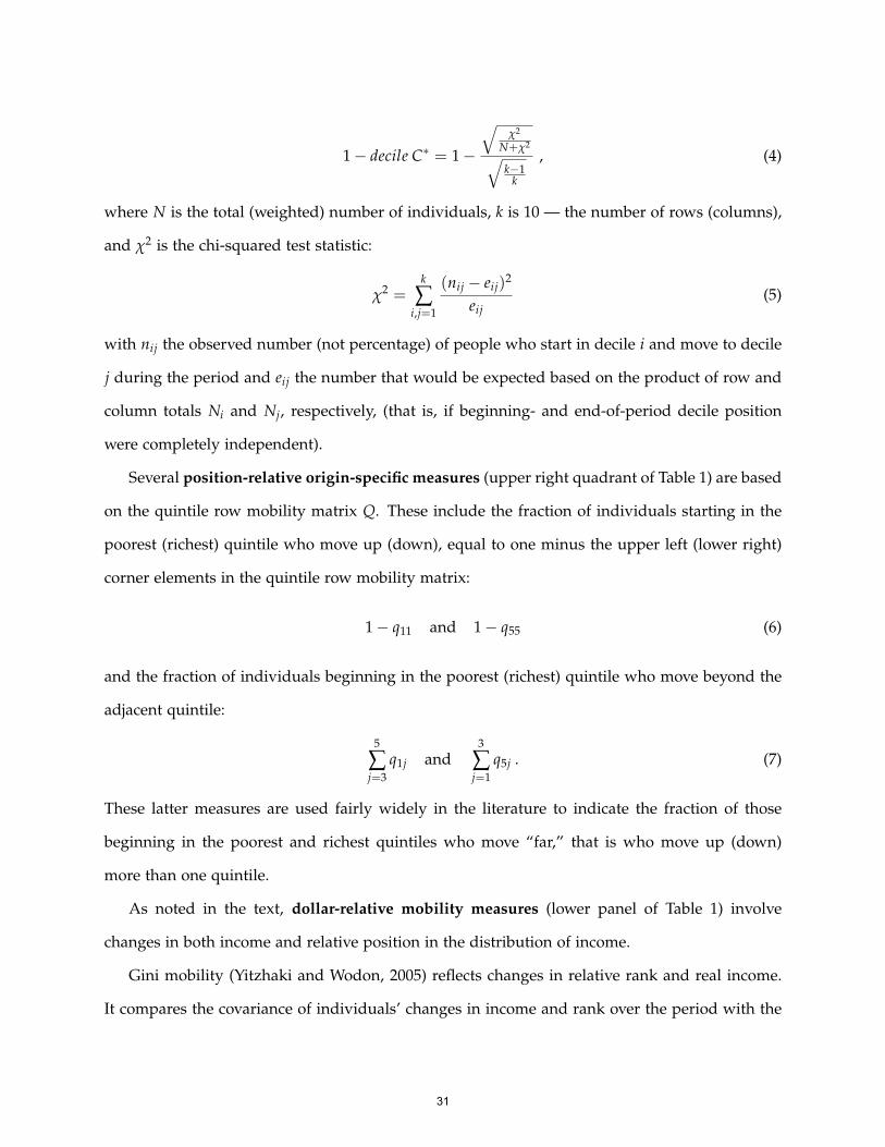
1− decile C∗ = 1−

√χ2

N+χ2√k−1

k

, (4)

where N is the total (weighted) number of individuals, k is 10 — the number of rows (columns),

and χ2 is the chi-squared test statistic:

χ2 =k

∑i,j=1

(nij − eij)2

eij(5)

with nij the observed number (not percentage) of people who start in decile i and move to decile

j during the period and eij the number that would be expected based on the product of row and

column totals Ni and Nj, respectively, (that is, if beginning- and end-of-period decile position

were completely independent).

Several position-relative origin-specific measures (upper right quadrant of Table 1) are based

on the quintile row mobility matrix Q. These include the fraction of individuals starting in the

poorest (richest) quintile who move up (down), equal to one minus the upper left (lower right)

corner elements in the quintile row mobility matrix:

1− q11 and 1− q55 (6)

and the fraction of individuals beginning in the poorest (richest) quintile who move beyond the

adjacent quintile:

5

∑j=3

q1j and3

∑j=1

q5j . (7)

These latter measures are used fairly widely in the literature to indicate the fraction of those

beginning in the poorest and richest quintiles who move “far,” that is who move up (down)

more than one quintile.

As noted in the text, dollar-relative mobility measures (lower panel of Table 1) involve

changes in both income and relative position in the distribution of income.

Gini mobility (Yitzhaki and Wodon, 2005) reflects changes in relative rank and real income.

It compares the covariance of individuals’ changes in income and rank over the period with the

31

covariances of income and rank at the start and the end of the period:4

N

∑i=1

(yie

µe–

yib

µb

)(Rie

N–

Rib

N

)N

∑i=1

(yie

µe– 1

)Rie

N+

N

∑i=1

(yib

µb– 1

)Rib

N

, (8)

where µb and µe are mean incomes at the beginning and end of the period, and Rib and Rie are

the rank of individual i in the beginning- and end-of-period distributions, from poorest (lowest

rank) to richest (highest rank). Yitzhaki and Wodon developed their measure to provide (along

with the Gini index of inequality) “an overall consistent framework for the analysis of mobility

[and] inequality”; they cite examples of job rotations and the distribution of income over the life

cycle, in which snapshot measures of inequality may give misleading indications of longer-term

inequality that their Gini mobility measure will correct. Note from the numerator expression

that if either an individual’s relative income or his/her rank does not change, the contribution to

Gini mobility is zero.

The elasticity of end-of-period income with respect to beginning-of-period income is the most

widely used measure of intergenerational income mobility (typically used in examining the de-

pendence of a man’s earnings on his father’s earnings at a similar life-stage). The elasticity is the

estimated coefficient in a regression of the logarithm of end-of-period income on the logarithm of

beginning of-period income. Subtracting the elasticity from one makes the measure higher when

mobility is higher — end-of-period income is less tightly tied to beginning-of-period income.

The Fields (2008) mobility-as-equalizer statistic measures whether the average (or sum) of

beginning-of-period and end-of-period income is more or less equal than beginning-of-period

income:

Fields MAE = 1− I(yib + yie)

I(yib), (9)

where yib and yie are beginning- and end-of-period income for individual i and I(.) is the Gini

(or other) index of inequality across all incomes. This measure has a directional aspect, in that

4They call it the Gini index of mobility because the Gini index of inequality is proportional to the covariance ofincome and rank.

32

it indicates the degree to which mobility equalizes average income compared with beginning-

year income. The index takes on larger positive values (closer to one) when average incomes

are more equally distributed than base-year incomes and becomes negative when the inequality

of end-year income is so much greater than that of beginning-year income that average of those

two incomes is less equally distributed than beginning-year income (that is, end-year inequality

overwhelms the equalizing power of averaging two years of income).5

Absolute quintile mobility can be characterized via absolute transition and mobility matrices

like their relative counterparts P and Q above, where Bp is a 5 x 5 absolute quintile transition

matrix consisting of elements bpij indicating the fraction of all individuals who begin in quintile

i and end in group j, where group j is defined by the real income range of beginning-of-period

quintile j. Similarly, absolute mobility matrix Bq consists of elements bqij indicating the fraction

of individuals starting in quintile i who end in group j. The absolute quintile mobility mea-

sure tallies the percentage of all individuals who move out of their beginning-of-period absolute

quintile:

1−5

∑k=1

bpkk . (10)

Shorrocks (1978a) proposes a measure of “the degree to which equalization occurs as the

observation period is extended”; it compares the inequality of long-term income (over t years)

with the (weighted average) inequality of single-year income (to produce a measure of rigidity,

R) and scales it to increase with mobility by subtracting the ratio from one:

Shorrocks M = 1− R = 1−I(yi1 + yi2 + ... + yit)

t

∑j=1

µj ∗ I(yij)

/ t

∑j=1

µj

, (11)

where I(.), as above, is an index of inequality; yi1, yi2, ...yit is the income of individual i in year

1 through year t (year 1 can be seen as year b, and year t as year e). For this measure, three

5A later paper (Fields et al., 2007) includes all years in the period, not just beginning and end years in this measure,but it is difficult to interpret the directional aspect of the measure (which Fields stresses) when multiple post-base-year incomes are included; in addition, only the denominators would distinguish Shorrocks M (see below) and FieldsMAE with the multi-year approach. Thus, the beginning- and end-year formulation of the Fields measure is usedhere.

33

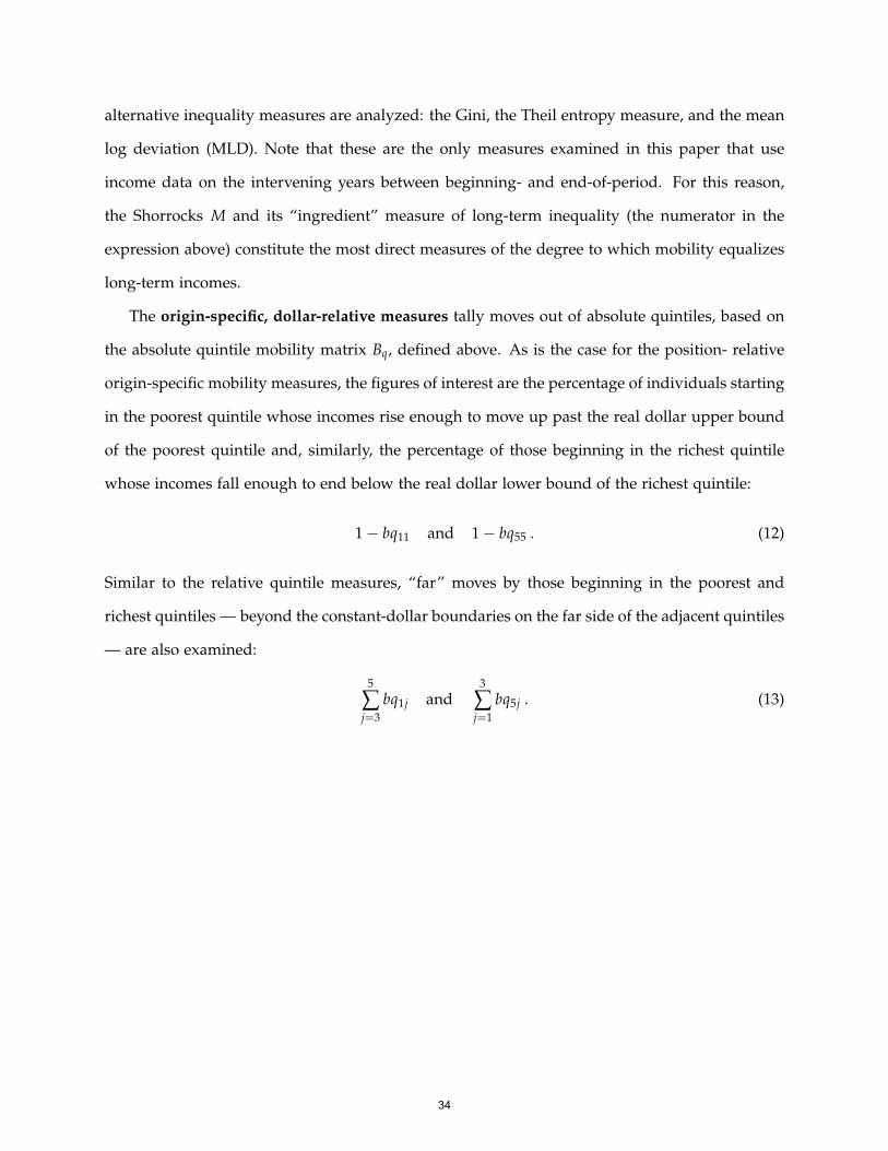
alternative inequality measures are analyzed: the Gini, the Theil entropy measure, and the mean

log deviation (MLD). Note that these are the only measures examined in this paper that use

income data on the intervening years between beginning- and end-of-period. For this reason,

the Shorrocks M and its “ingredient” measure of long-term inequality (the numerator in the

expression above) constitute the most direct measures of the degree to which mobility equalizes

long-term incomes.

The origin-specific, dollar-relative measures tally moves out of absolute quintiles, based on

the absolute quintile mobility matrix Bq, defined above. As is the case for the position- relative

origin-specific mobility measures, the figures of interest are the percentage of individuals starting

in the poorest quintile whose incomes rise enough to move up past the real dollar upper bound

of the poorest quintile and, similarly, the percentage of those beginning in the richest quintile

whose incomes fall enough to end below the real dollar lower bound of the richest quintile:

1− bq11 and 1− bq55 . (12)

Similar to the relative quintile measures, “far” moves by those beginning in the poorest and

richest quintiles — beyond the constant-dollar boundaries on the far side of the adjacent quintiles

— are also examined:

5

∑j=3

bq1j and3

∑j=1

bq5j . (13)

34

References

Acs, Gregory and Seth Zimmerman. 2008a. “U.S. Intragenerational Economic Mobility from 1984 to 2004: Trends and Implications.” Report from the Economic Mobility Project (October).

Acs, Gregory and Seth Zimmerman. 2008b. “Like Watching Grass Grow? Assessing Changes in U.S. Intragenerational Economic Mobility Over the Past Two Decades.” [a more detailed version of 2008a] (November).

Auten, Gerald and Geoffrey Gee. 2009. “Income Mobility in the United States: New Evidence from Income Tax Data.” National Tax Journal 62(2): 301–328 (June).

Auten, Gerald and Geoffrey Gee. 2007. “Income Mobility in the U. S. from 1996 to 2005.” Report of the Department of the Treasury (November 13).

Bradbury, Katharine and Jane Katz. 2002. “Are lifetime incomes growing more unequal? Looking at new evidence on family income mobility.” Regional Review 12(4): 2–5 (Quarter 4.

Burkhauser, Richard V., Jeff Larrimore, and Kosali I Simon. 2011. “A ‘Second Opinion’ on the Economic Health of the American Middle Class.” National Bureau of Economic Research Working Paper 17164 (June).

Burkhauser, Richard V. and Kenneth A. Couch. 2009. “Intra-Generational Inequality and Intertemporal Mobility.” in The Oxford Handbook of Income Inequality, ed. Wiemar Salverda, Brian Nolan, and Timothy Smeeding, Chapter 21: 522–545. Oxford University Press.

Burkhauser, Richard V., Shuaizhang Feng, and Stephen P. Jenkins. 2009. “Using the P90/P10 Index to Measure U.S. Inequality Trends with Current Population Survey Data: A View from Inside the Census Bureau Vaults.” Review of Income and Wealth 55(1): 166–185 (March).

Burkhauser, Richard V., Timothy M. Smeeding, and Joachim Merz. 1996. “Relative Inequality and Poverty in Germany and the United States Using Alternative Equivalence Scales.” Review of Income and Wealth 42(4): 381-400 (December).

Carroll, Robert, David Joulfaian, and Mark Rider. 2006. "Income Mobility: The Recent American Experience." Georgia State University, Andrew Young School of Policy Studies Working Paper No. 06-20.

Cornell University. Cross-National Equivalent File, U.S. data based on the Panel Study of Income Dynamics. Electronic data files.

Economic Mobility Project. 2009. “[Summary of] Findings from a National Survey & Focus Groups on Economic Mobility.” (March 12).

Fields, Gary S. 2008. “Income Mobility.” entry in The New Palgrave Dictionary of Economics Second Edition, Online, ed. Steven N. Durlauf and Lawrence E. Blume: Palgrave Macmillan.

Fields, Gary S., Robert Duval Hernández, Samuel Freije, María Laura Sánchez Puerta, Omar Arias, Juliano Assunção. 2007. “Intragenerational Income Mobility in Latin America.” Economía 7(2): 101–154 (Spring).

Fields, Gary S. and Efe A. Ok. 2001. “The Measurement of Income Mobility: An Introduction to the Literature.” in Handbook on Income Inequality Measurement ed. J. Silber, Chapter 19:

35

557–598. Boston, MA: Kluwer. Fields, Gary S. and Efe A. Ok. 1999. “Measuring Movement of Incomes.” Economica 66: 455-71. Gittleman, Maury, and Mary Joyce. 1999. “Have Family Income Mobility Patterns Changed?”

Demography 36(3): 299–314 (August). Gottschalk, Peter, and Sheldon Danziger. 2001. "Income Mobility and Exits from Poverty of

American Children, 1970–1992." in The Dynamics of Child Poverty in Industrialised Countries, ed. Bruce Bradbury, Stephen P. Jenkins, and John Micklewright, Cambridge University Press.

Gottschalk, Peter, and Sheldon Danziger. 2005. “Inequality of Wage Rates, Earnings, and Family Income in the United States, 1975–2002.” Review of Income and Wealth. 51(2): 231–254 (June).

Holt, Steve. 2011. “Ten Years of the EITC Movement: Making Work Pay Then and Now.” Brookings Institution Metropolitan Opportunity Series (April).

Holt, Steve. 2006. “The Earned Income Tax Credit at Age 30: What We Know.” The Brookings Institution Research Brief (February).

Hungerford, Thomas L. 2011. “How Income Mobility Affects Income Inequality: U.S. Evidence in the 1980s and the 1990s.” Journal of Income Distribution, 20(1): 83–103.

Hungerford, Thomas L. 2008. “Income Inequality, Income Mobility, and Economic Policy: U.S. Trends in the 1980s and 1990s.” Congressional Research Service Report for Congress (April 4).

Hungerford, Thomas L. 1993. “U.S. Income Mobility in the Seventies and Eighties.” Review of Income and Wealth. 39(4): 403–417 (December).

Karoly, Lynn A. and Gary Burtless. 1995. “Demographic Change, Rising Earnings Inequality, and the Distribution of Personal Well-Being, 1959–1989.” Demography 32(3): 379–405 (August).

Piketty, Thomas and Emmanuel Saez. 2006. “How Progressive Is the U.S. Federal Tax System? A Historical and International Perspective.” National Bureau of Economic Research Working Paper 12404 (July).

Sawhill, Isabel, and Mark Condon. 1992. "Is U.S. Inequality Really Growing? Sorting Out the Fairness Question." Urban Institute Policy Bites 13 (June).

Shorrocks, Anthony. 1978a. “Income Inequality and Income Mobility.” Journal of Economic Theory 19: 376–393.

Shorrocks, Anthony. 1978b. “The Measurement of Mobility” Econometrica 46(5): 1013–1024 (September).

U.S. Census Bureau. 2007. “The Effect of Taxes and Transfers on Income and Poverty in the United States: 2005.” Current Population Reports P60-232 (March).

Van Kerm, Philippe. 2004. “What Lies behind Income Mobility? Reranking and Distributional Change in Belgium, Western Germany and the USA.” Economica 71(282): 223–239 (May).

Yitzhaki, Shlomo and Quentin Wodon. 2005. “Mobility, Inequality, and Horizontal Equity.” In Research on Economic Inequality, Studies on Economic Well-Being: Essays in Honor of John P. Formby, ed. Y. Amiel and J.A. Bishop, Emerald Group Publishing: Journal of Economic Literature 12: 179–199.

36

Table 1. Measures of mobility analyzed in this paperOVERALL ORIGIN-SPECIFIC

• Decile mobility • Fraction of poorest (richest) quintile

• Per capita decile movement who move up (down)

POSITION- • Shorrocks M-hat for quintiles • Fraction of poorest (richest) quintile

RELATIVE • Rank correlation (inverse) who move “far” -- to middle or farther

• Decile adjusted contingency quintiles

coefficient C* (inverse)

• Gini mobility • Fraction of poorest (richest) quintile

• Elasticity of end-year income who move above (below) that

with respect to beginning- quintile’s real ceiling (floor)

year income (inverse) • Fraction of poorest (richest) quintile

DOLLAR- • Fields directional mobility-as- who move “far” in real terms --

RELATIVE -equalizer (MAE) above (below) the real dollar

• Absolute quintile mobility ceiling (floor) of adjacent quintile

• Shorrocks M (=1-R) equalization

with time (based on Gini, Theil entropy,

and mean log deviation)

• Inequality of long-term income

Note: See text for discussion and appendix for definitions and sources.

37

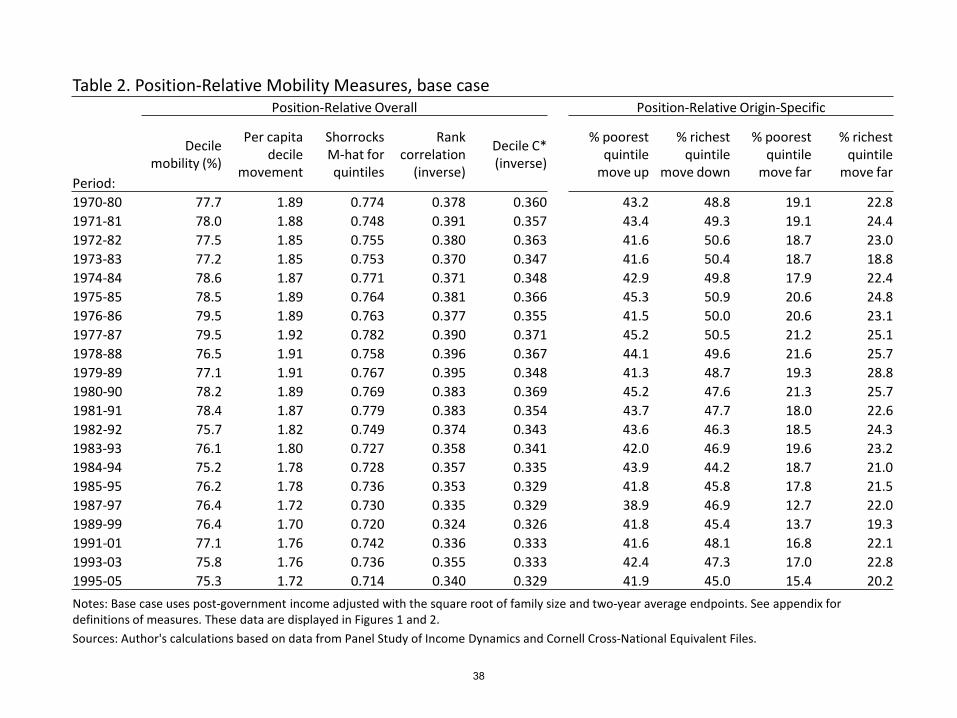
Table 2. Position-Relative Mobility Measures, base casePosition-Relative Overall Position-Relative Origin-Specific

Period:

Decile mobility (%)

Per capita decile

movement

ShorrocksM-hat for quintiles

Rank correlation

(inverse)

Decile C* (inverse)

% poorest quintile

move up

% richest quintile

move down

% poorest quintile

move far

% richest quintile

move far

1970-80 77.7 1.89 0.774 0.378 0.360 43.2 48.8 19.1 22.81971-81 78.0 1.88 0.748 0.391 0.357 43.4 49.3 19.1 24.41972-82 77.5 1.85 0.755 0.380 0.363 41.6 50.6 18.7 23.01973-83 77.2 1.85 0.753 0.370 0.347 41.6 50.4 18.7 18.81974-84 78.6 1.87 0.771 0.371 0.348 42.9 49.8 17.9 22.41975-85 78.5 1.89 0.764 0.381 0.366 45.3 50.9 20.6 24.81976-86 79.5 1.89 0.763 0.377 0.355 41.5 50.0 20.6 23.11977-87 79.5 1.92 0.782 0.390 0.371 45.2 50.5 21.2 25.11978-88 76.5 1.91 0.758 0.396 0.367 44.1 49.6 21.6 25.71979-89 77.1 1.91 0.767 0.395 0.348 41.3 48.7 19.3 28.81980-90 78.2 1.89 0.769 0.383 0.369 45.2 47.6 21.3 25.71981-91 78.4 1.87 0.779 0.383 0.354 43.7 47.7 18.0 22.61982-92 75.7 1.82 0.749 0.374 0.343 43.6 46.3 18.5 24.31983-93 76.1 1.80 0.727 0.358 0.341 42.0 46.9 19.6 23.21984-94 75.2 1.78 0.728 0.357 0.335 43.9 44.2 18.7 21.01985-95 76.2 1.78 0.736 0.353 0.329 41.8 45.8 17.8 21.51987-97 76.4 1.72 0.730 0.335 0.329 38.9 46.9 12.7 22.01989-99 76.4 1.70 0.720 0.324 0.326 41.8 45.4 13.7 19.31991-01 77.1 1.76 0.742 0.336 0.333 41.6 48.1 16.8 22.11993-03 75.8 1.76 0.736 0.355 0.333 42.4 47.3 17.0 22.81995-05 75.3 1.72 0.714 0.340 0.329 41.9 45.0 15.4 20.2

Notes: Base case uses post-government income adjusted with the square root of family size and two-year average endpoints. See appendix for definitions of measures. These data are displayed in Figures 1 and 2.Sources: Author's calculations based on data from Panel Study of Income Dynamics and Cornell Cross-National Equivalent Files.

38

Table 3. Dollar-Relative Mobility Measures, base caseDollar-Relative Overall Dollar-Relative Origin-Specific

Period:

Gini mobilityIncome

elasticity (inverse)

Fields MAEAbsolute

quintile mobility (%)

% poorest quintile rise

past real ceiling

% richest quintile fall

past real floor

% poorest quintile rise

far in real terms

% richest quintile fall far

in real terms

1970-80 0.370 0.352 0.0843 63.5 56.5 27.4 34.3 10.21971-81 0.385 0.350 0.0789 63.0 53.0 34.2 26.0 14.61972-82 0.371 0.312 0.0685 61.5 48.8 38.6 24.6 18.51973-83 0.359 0.283 0.0575 61.7 48.6 36.8 23.2 12.91974-84 0.355 0.233 0.0341 62.1 47.4 31.2 26.5 14.11975-85 0.367 0.283 0.0538 62.7 49.6 35.4 30.8 14.11976-86 0.363 0.233 0.0246 61.5 49.4 27.6 31.5 11.91977-87 0.376 0.280 0.0372 62.6 51.9 30.1 31.3 14.01978-88 0.377 0.245 0.0027 65.8 54.0 28.4 34.2 11.31979-89 0.378 0.250 0.0137 65.4 56.1 29.9 31.5 13.41980-90 0.364 0.240 0.0038 65.4 58.9 24.7 35.9 11.91981-91 0.369 0.286 0.0335 66.1 61.3 20.8 35.0 9.81982-92 0.348 0.271 0.0200 66.1 62.0 24.6 35.0 12.51983-93 0.345 0.262 0.0377 64.8 60.9 21.8 33.1 10.61984-94 0.346 0.273 0.0293 62.3 56.1 24.2 28.5 10.41985-95 0.343 0.271 0.0354 63.3 56.9 22.6 33.2 8.11987-97 0.331 0.280 0.0511 62.3 56.6 23.2 27.6 10.91989-99 0.324 0.278 0.0515 63.7 61.4 23.8 33.0 7.01991-01 0.339 0.289 0.0609 63.6 56.9 26.4 31.7 9.31993-03 0.353 0.299 0.0576 64.1 59.9 24.7 33.8 9.81995-05 0.334 0.246 0.0189 63.3 55.1 23.0 27.9 9.0

Notes: Base case uses post-government income adjusted with the square root of family size and two-year average endpoints. See appendix for definitions of measures. These data are displayed in Figures 3 and 4.Sources: Author's calculations based on data from Panel Study of Income Dynamics and Cornell Cross-National Equivalent Files.

39

Table 4. Mobility Measured as Equalization of Long-Term Income, base caseShorrocks M: reduction in inequality attributable

to mobility (%)Inequality of long-term income

Period:Gini Theil entropy

Mean log deviation

Gini Theil entropyMean log deviation

1969-79 13.0 24.9 26.9 0.220 0.077 0.0821970-80 13.6 25.9 27.7 0.220 0.078 0.0821971-81 13.4 25.8 27.7 0.219 0.076 0.0811972-82 13.8 26.5 28.4 0.221 0.078 0.0831973-83 12.9 25.0 27.3 0.222 0.079 0.0831974-84 12.9 24.8 26.7 0.228 0.083 0.0881975-85 12.7 24.8 27.3 0.230 0.084 0.0891976-86 13.0 25.2 27.2 0.230 0.085 0.0901977-87 12.9 25.1 27.2 0.232 0.086 0.0921978-88 12.6 24.6 26.3 0.236 0.089 0.0951979-89 12.5 24.6 26.7 0.240 0.092 0.0981980-90 12.3 23.9 25.9 0.242 0.095 0.1001981-91 12.0 23.4 25.8 0.246 0.098 0.1041982-92 12.0 23.4 25.8 0.250 0.101 0.1071983-93 12.4 24.2 26.7 0.252 0.103 0.1091984-94 12.2 24.0 26.5 0.254 0.104 0.1111985-95 12.1 24.0 26.4 0.256 0.105 0.1131986-96 12.9 25.4 27.8 0.252 0.102 0.1101988-98 13.1 26.1 28.7 0.255 0.104 0.1121990-00 13.3 26.9 29.5 0.258 0.107 0.1151992-02 14.3 28.4 31.8 0.258 0.107 0.1171994-04 14.2 28.4 31.8 0.263 0.112 0.1201996-06 13.5 27.7 32.0 0.278 0.125 0.135Notes: Base case uses post-government income adjusted with the square root of family size. See appendix for definitions of measures. "Long-term" defined as 10-year period, averaging income over every other year within period. These data are displayed in Figures 5 and 7.Sources: Author's calculations based on data from Panel Study of Income Dynamics and Cornell Cross-National Equivalent Files.

40

Table 5. Significance tests for changes over time

MeasureType of estimate

Periods & levels Difference S.E.

Position-Relative Overall Mobility 1977-87 1995-05Decile mobility (%) Logit 79.5 75.3 -0.240*** (0.077)Per capita decile movement OLS 1.92 1.72 -0.201*** (0.053)Shorrocks M-hat for quintiles Bootstrap 0.782 0.714 -0.068*** (0.021)Rank correlation (inverse) OLS 0.390 0.340 -0.049** (0.024)Decile C* (inverse) Bootstrap 0.371 0.329 -0.043*** (0.016)

Position-Relative Origin-Specific Mobility 1977-87 1995-05% poorest quintile move up Logit 45.2 41.9 -0.133 (0.138)% richest quintile move down Logit 50.5 45.0 -0.222 (0.153)% poorest quintile move far Logit 21.2 15.4 -0.391** (0.182)% richest quintile move far Logit 25.1 20.2 -0.281 (0.182)

Dollar-Relative Overall Mobility 1981-91 1995-05Income elasticity (inverse) OLS 0.369 0.334 -0.035 (0.031)Gini mobility Bootstrap 0.286 0.246 -0.041* (0.021)Fields MAE Bootstrap 0.0335 0.0189 -0.015 (0.016)Absolute quintile mobility (%) Logit 66.1 63.3 -0.123* (0.065)

Dollar-Relative Origin-Specific Mobility 1981-91 1995-05% poorest quintile rise past real ceiling Logit 61.3 55.1 -0.252* (0.135)% richest quintile fall past real floor Logit 20.8 23.0 0.127 (0.172)% poorest quintile rise far in real terms Logit 35.0 27.9 -0.333** (0.150)% richest quintile fall far in real terms Logit 9.83 9.00 -0.098 (0.238)

Notes: Logit differences are expressed in terms of log odds. Clustered standard errors are reported in parentheses (see text for details). Asterisks denote significance as follows: * p<0.10, ** p<0.05, *** p<0.01

Sources: Author's calculations based on data from Panel Study of Income Dynamics and Cornell Cross-National Equivalent Files.

41

0.30

0.32

0.34

0.36

0.38

0.40

0.42

Figure 1. Position-relative overall mobility measuresBase case

M-hat/2

Per capita decile movement/5

Decile C* (inverse)

Rank correlation (inverse)

Decile mobility/2

Note: Base case uses post-government income adjusted with the square root of family size and two-year average endpoints. See appendix for definitions of measures. These data are listed in Table 2. Source: Author’s calculations based on Panel Study of Income Dynamics and Cornell University Cross National Equivalent File.

42

10%

15%

20%

25%

30%

35%

40%

45%

50%

55%

Position-relative origin-specific mobility for poorest and richest quintiles Base case

% of richest quintile who move down

% of poorest quintile who move far

% of richest quintile who move far

Figure 2.

% of poorest quintile who move up

Note and source: see Figure 1.43

-0.05

0.00

0.05

0.10

0.15

0.20

0.25

0.30

0.10

0.15

0.20

0.25

0.30

0.35

0.40

0.45

Figure 3. Dollar-relative overall mobility measuresBase case

Two upper lines, left axis

Gini mobility

Income elasticity (inverse)

Fields MAE, right axis

Note and source: see Figure 1. These data are listed in Table 3.44

-30%

-20%

-10%

0%

10%

20%

30%

40%

0%

10%

20%

30%

40%

50%

60%

70%

Figure 4. Absolute quintile mobility and income growthBase case

Real income growth, right axis

Absolute quintile mobility %

% of poorest quintile who rise past real ceiling

% of richest quintile who fall past real floor

% of poorest quintile who rise far in real terms

% of richest quintile who fall far in real terms

Note and source: see Figure 1. These data are listed in Table 3.45

10%

15%

20%

15%

20%

25%

30%

35%

Shorrocks M: Degree to which 10-year mobility offsets 1-year inequalityBase case

Figure 5.

Two upper lines, left axis

Mean log deviation

Theil

Gini, right axis

Note: Base case uses post-government income adjusted with the square root of family size and every-other-year income within 10-year period. See appendix for definitions of measures. These data are listed in Table 4. Source: Author’s calculations based on Panel Study of Income Dynamics and Cornell University Cross National Equivalent File.

46

0.20

0.25

0.30

0.35

0.40

0.45

0.50

0.55

0.60

1967 1970 1973 1976 1979 1982 1985 1988 1991 1994 1997 2000 2003 2006 2009

Figure 6. U.S. household income inequality, CPS data

Theil

Note: Discontinuities between 1992 and 1993 reflect changes in data collection methods and increases in income limits for recording data.Source: U.S. Bureau of the Census, Table A-1. Selected Measures of Household Income Dispersion, 1967-2009. Current Population Reports, Series P-60; see http://www.census.gov/hhes/www/income/data/historical/inequality/taba2.pdf .

Mean log deviation

Gini

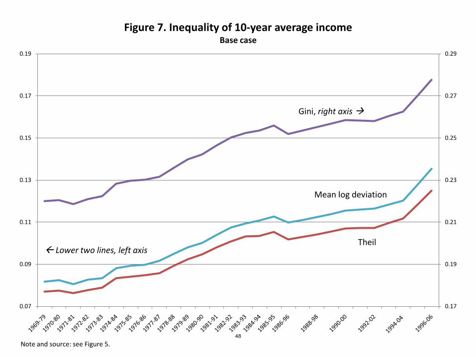
0.17

0.19

0.21

0.23

0.25

0.27

0.29

0.07

0.09

0.11

0.13

0.15

0.17

0.19

Figure 7. Inequality of 10-year average incomeBase case

Gini, right axis

Mean log deviation

Theil Lower two lines, left axis

Note and source: see Figure 5. 48

0.00

0.02

0.04

0.06

0.08

0.10

0.12

0.14

0.16

0.18

0.00

0.05

0.10

0.15

0.20

0.25

0.30

0.35

0.40

0.45

Lower 2 lines, right axis

Upper 3 lines, left axis

Figure 8. Position-relative measures of overall "mobility" from pre-government income to post-government income

Per family decile movement

Decile mobility

M-hat

Decile C* (inverse)

Rank correlation (inverse)

Note: Mobility as “movement” from pre-government income position to post-government income position; incomes are adjusted using square root of family size. See appendix for definitions of measures. Source: Author’s calculations based on Panel Study of Income Dynamics and Cornell University Cross National Equivalent File.

49

0.29

0.31

0.33

0.35

0.37

0.39

0.41

Figure 9. Position-relative mobility measures, pre-government income(overlap sample)

Decile mobility/2

M-hat/2

Decile C* (inverse)

Per family decile movement/5Rank correlation (inverse)

Note: Based on pre-government income adjusted with the square root of family size and two-year average endpoints. Overlap sample includes observations present in both pre- and post-government trimmed samples; see text. See appendix for definitions of measures. Source: Author’s calculations based on Panel Study of Income Dynamics and Cornell University Cross National Equivalent File.

0%

10%

20%

30%

40%

50%

60%

70%

Figure 10. Absolute quintile mobility measures, pre-government income(overlap sample)

Absolute quintile mobility

% of poorest quintile who rise past real ceiling

% of richest quintile who fall past real floor

% of richest quintile who fall far in real terms

% of poorest quintile who rise far in real terms

Note and source: see Figure 9. 51