Trends in systolic and cellular computation · PDF fileTrends in systolic and cellular computation ... the singular value decomposition, ... algorithms onto systolic arrays

Journal of Computational and Applied Mathematics 38 (1991) 297-321 North-Holland

297

Trends in systolic and cellular computation

George Miel * Hughes Research Laboratories, 3011 Malibu Canyon Road, Malibu, CA 90265, United States

Received 16 October 1990 Revised 27 November 1990

Abstract

Miel, G., Trends in systolic and cellular computation, Journal of Computational and Applied Mathematics 38 (1991) 297-321.

A profile is given of current research, as it pertains to computational mathematics, on Very Large Scale Integration (VLSI) array processors. In this type of parallel computers, the cells of the array operate in Single Instruction Multiple Data (SIMD) mode and algorithms are executed in systolic or cellular fashion. The focus of the presentation is on linear algebraic techniques. A systolization process is illustrated by matching an arbitrary gaxpy operation onto a fixed-size square array processor. Two recent systolic methods, for solving systems of linear equations, one iterative and the other direct, are described. A cellular algorithm for a fast Fourier transform, based on a new implementation on rectangular array processors of the perfect shuffle permutation, is then derived. Using annotated lists of recent references, snapshots of active research areas are given on systolic linear solvers, the singular value decomposition, artificial neural networks, and the simulated annealing algorithm.

Keywords: Parallel computational linear algebra, mesh array processors, systolic and cellular algorithms.

1. Introduction

Very Large Scale Integration (VLSI) mesh array processors have received considerable attention for applications requiring high throughput. In this type of parallel computers, the cells of the array operate in Single Instruction Multiple Data (SIMD) mode and algorithms are executed in systolic or cellular fashion. Two areas of applications for VLSI mesh arrays are in signal processing and in scientific computing. In the former case, the mesh array is used as a special-purpose processor embedded in a sensor system. In the second case, it serves as an accelerator, performing matrix-based and other “locally recursive” computations involved in large scale simulations, under the control of a conventional general-purpose computer. For certain applications, the resulting throughput is potentially that of a supercomputer at a fraction of the cost.

* Present address: Department of Mathematical Sciences (or Department of Computer Science), University of Nevada, Las Vegas, NV 89154, United States.

0377-0427/91/$03.50 0 1991 - Elsevier Science Publishers B.V. All rights reserved

298 G. Mid / Systolic and cellular computation

An array processor has two modes of operation: cellular and systolic. In the cellular mode, the input data are first loaded into the array, then processed in unison, the results are then unloaded from the array. and a similar cycle starts anew. In the systolic mode of operation, the loading, computing and unloading occur concurrently. In this mode every processor regularly pumps data in and out, each time performing a short computation, with the data rhythmically flowing through the network.

Due to the importance of linear-algebraic methods in scientific computing. matrix problems have become preferred benchmarks for high-performance computers [18,19]. A survey of parallel algorithms for dense linear-algebraic computation was recently presented in [25]. A comprehen- sive review of iterative methods has been presented in [67]. Both surveys concentrate on commercially available computers, consisting of a modest number of processors, with shared- memory multivector units like the CRAY-2 or distributed memory like the hypercube. Surpriz- ingly. the surveys hardly consider massively parallel-array processors, which in fact are ideally suited for matrix computation.

Linear-algebraic operations have properties of locality, recursiveness and regularity that match well the fine-grain parallelism of array processors. When the dimension of the problem corresponds to the dimension of the array processor, a matrix operation can have very low overhead in communication and synchronization. Speiser and Whitehouse [Sl] have shown that computational requirements for many real-time signal processing tasks (such as adaptive filtering, beamforming, cross-ambiguity calculations, data compression, etc.) may be reduced to a com- mon set of linear-algebraic operations. It is no surprise, therefore, that there is considerable research activity on matrix-based cellular and systolic computation.

Our goal is to portray a profile of such activity by describing recent algorithms, both systolic and cellular. The outline of the paper is as follows. Section 2 illustrates a systolization process by matching an arbitrary gaxpy operation onto a fixed-size square array processor. The next section describes two systolic methods, one iterative and the other direct, for solving systems of linear equations. Section 4 derives a cellular algorithm for a fast Fourier transform, based on a new implementation on rectangular-array processors of the perfect-shuffle permutation. Finally, Section 5 gives snapshots of active research areas, using annotated lists of recent references on systolic linear solvers, the singular value decomposition, artificial neural networks and the simulated annealing algorithm. Our notation is standard with !RH” denoting Euclidean n-space and !N mxn representing the space of real m X n matrices. The subscript t denotes transposition of a matrix.

For the benefit of the reader not familiar with array processors, we briefly describe an illustrative architecture, namely, a prototype systolic/cellular processor [65,71] built at Hughes Research Laboratories. As shown in Fig. 1, the system consists of a host processor, a back-end array processor coupled with a corresponding array memory, and a controlIer with related program memory. The host coordinates such tasks as loading data into the array processor. initiating the execution of programs, and unloading results from the array processor. The array processor consists of 256 processing cells configured as a 16 X 16 square mesh. The cells operate in SIMD mode. A masking capability allows turning off a given subset of cells during execution. Each interior cell is connected to its four nearest neighbors via two horizontal and two vertical connections. There is also a wraparound connection between the two ends of each row. Each processing cell possesses a local memory and multiple functional units for computation. Boundary cells on one side can optionally have a hardwired square root in order to accelerate certain

G. Miel / Systolic and cellular computation 299

DUALPORT ARRAY MEMORY tl I

HOST BUS I

I

INTERFACE

COPROCESSOR BUS I

CONTROLLER

PROCESSOR ARRAY

Fig. 1. Diagram of the Hughes prototype.

operations, for example, Givens rotations in the solution of linear systems [62]. The program memory is separate from the data memory. The latter is partitioned into 16 columns, each affiliated with a corresponding column of the array processor. This memory has two independent ports, one of which is used to load data into the array processor, the other to store results back into memory.

The prototype demonstrated the viability of the hardware design. Evolutionary models, currently under study, enhance miscellaneous capabilities, and increase the size of the array processor while preserving its square geometry and connectivity. A variety of algorithms have been mapped onto such architectures by Hughes researchers [55-57,61-64,70,72,73,77].

Table 1 shows comparative peak performance parameters for a CRAY supercomputer with 4 processors and two systolic array processors of different sizes.

The processors respectively have a clock rate of 105, 8, 16 and a memory cycle of 26, 16.7, 26 all measured in MHz. In both array processors, the word length is 32 bits and each cell has two multipliers, two adders, a divider, and a selector, four of which can operate concurrently. The 16 X 16 model uses fixed-point arithmetic. The memory Bandwidth, MIPS and MFLOPS parameters are compared to those of the CRAY-IS normalized to 1. The benchmark is the time in milliseconds to solve a 100 X 100 system of linear equations. The CRAY uses FORTRAN routines DGEFA and DGESL from LINPACK, with Rolled BLAS calls, compiled with the CFT

Table 1

Processor Bandwidth MIPS MFLOPS Benchmark

CIUY X-MP4 16 x 16 array 128 X 128 array

32 5.3 5.3 14 0.13 14.6 - 31 3.2 1872 4369 3

300 G. Mel / Systolic and cehlar computation

vectorizing compiler [18]. The two array processors use an assembly-coded version of the systolized partitioned Faddeev algorithm [62] described in the sequel.

2. Systolic gaxpy computation

Given an algorithm satisfying prerequisite properties, the process of deriving a model of a systolic array for executing the algorithm is called a mapping. Diverse methods exist for mapping algorithms onto systolic arrays. Cape110 an Steiglitz use geometric [9] and linear space-time transformations [lo]. Kung [37] proposes a technique, which we use in part in the sequel, based on data dependence and signal flow graphs. Leiserson [47] presents a scheme for minimizing the number of delay elements. Moldovan [58] uses a formalism based on transformation of index sets and data dependence vectors. Navarro et al. [66] study partitioning of matrix operations onto fixed-size array processors. Quinton [74] produces a method for algorithms that can be expressed as a set of uniform recurrence relations. Other contributions have been made.

Although the solutions to mapping problems promote conceptual understanding of time-space issues at hand, the process by itself is only of partial use in practical situations that require the extraction of systolic algorithms for a given specific architecture. The inverse of the mapping problem, in which one starts with an array processor and wishes to get systolic algorithms for it, is called the constrained mapping or matching problem. The former term denotes the process of fitting algorithms under constraints of array topology, number of cells, global and local memory sizes, etc. A special case of the matching problem occurs when the size of the dependence graph of the algorithm is bigger than the size of the array processor. This is the so-called partitioning

problem. In this section, in order to illustrate how systolic algorithms are derived, we shall match a

simple linear-algebraic operation onto a fixed-size square array processor of the type described in Section 1. Specifically, our aim is to match an affine operation

z=Flx+y, AESrnXP, XE!RP, yf=!Rm, (1)

onto a square N X N systolic array, of fixed size N, with square mesh connectivity, whose primitive operation in each cell is a scalar multiply-add

ffP+v. (2)

In effect, we shall specify the equivalent of a BLAS2 primitive [25, Section 31 for the targeted architecture. The affine operation (1) is also called a gaxpy operation, a name that has its origin in the LINPACK software package. One can think of the term as a mnemonic for “general Ax plus y “. This operation, which may be viewed as an extension of the scalar operation (2), is in fact computed as a systematic combination of its scalar counterpart.

Our matching procedure proceeds in three steps. (1) The operation is mapped onto a linear array with N cells when p = N. (2) It is then partitioned onto the same linear array when p > N. (3) The partitioning is applied on each row of the N X N array.

The linear array with N cells in steps (1) and (2) may be viewed as one row of the square array.


2. I. Mapping

Assume that p = N. An algorithm for operation (1) can be expressed as follows: For i = 1, 2,.. ., m

For j = 1, 2,. . . , N x(i, j): = x(i - 1, j) z(i, j): = a(i, j)* x(i, j) + z(i, j - 1) End

End The inputs are a(i, j) = a,j, x(0, j) = xi, z(i, 0) =y, and the outputs are z(i, N) = zi. The right-hand side of the fourth statement is a primitive operation. With a view of systolizing the procedure, the algorithm is put in single assignment form (each indexed variable is assigned a single value) and transmittent variables x(i, j) and z( i, j) are used to localize all data dependencies. These transmittent variables will allow us to distribute the xi and zj values without broadcasting.

In order to systolize the algorithm, we apply the so-called canonical mapping methodology [37, Section 3.31. In this approach, three structures are successively developed:

(1) a dependence graph (DG) which shows the data dependencies in the algorithm; (2) a signal flow graph (SFG), which serves as an abstract model of the processor arrray,

obtained by operating on the DG; (3) and lastly, a systolic array design obtained by incorporating temporal considerations in the

SFG. We briefly describe each of these structures. The DG is a directed graph whose nodes are elements of the index space

{k=(i, j): l<i<m,l<j<N}

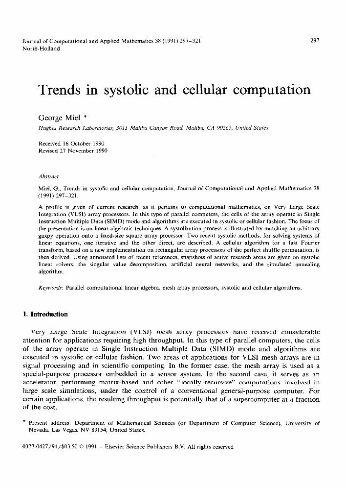
and whose edges denote data dependencies. An index point has incoming edges from all points it is directly dependent on. The DG for the affine operation with m = 4, N = 3 is shown in Fig. 2. The DG satisfies two prerequisites for the use of the canonical mapping methodology.

(1) The lengths of edges are independent of the problem size m, N. This property of the DG in fact formally defines a locally recursive algorithm. ---

(2) The DG is shift imaria+ in the sense that for index vectors k,, k,, k if a variable at q depends on a variable at q - k, then a variable at k, depends on a variable at & - k. Inputs and outputs at the border nodes are exempted from this requirement.

A graph with these properties represents a locally repetitive and homogeneous algorithm, well-suited for systematic systolization.

An SFG is also a directed graph. Nodes represent primitive operations and each edge denotes either a dependence relation or a time delay operator, in which case that edge is labelled with a capital letter D. In the SFG, primitive operations are assumed to require no execution time. Consequently, the derivation of time-space relations associated with pipelining are postponed to the third stage of the methodology. The SFG is obtained by operating on the DG. The nodes of the index space are assigned to nodes of the SFG and the order in which these nodes are to be executed is scheduled. These two steps proceed like this:

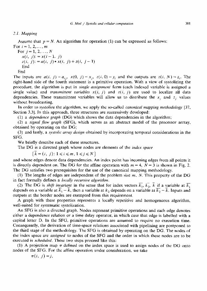
(1) A projection map 7~ defined on the index space is used to assign nodes of the DG onto nodes of the SFG. For the affine operation under consideration, we take

r(i, j) =j,

302 G. Mid / Systolic and relhdar computarion

Fig. 2. DG for a gaxpy operation.

namely, all the nodes along each vertical line of the DG are projected onto a single node of the SFG. See Fig. 3(a).

(2) An integer-valued map u defined on the index space is used to specify the order in which the nodes of the DG are to be executed. In our case.

u(i, j) =i+_j- 1.

Nties mapped onto the same integer, which fall on a line in the index space called an equirempural hyperplane. are to be executed at the same time. The set of integer values of u thus corresponds to a set of parallel hyperplanes in the index space. See Fig. 3(b).

PROJECTION I

& 0 D

@.)

Fig. 3. Transforming the DG to an SFG: (a) projection map n; (b) linear schedule u; (c) resulting SFG.


HYPERPLANE 6 ..__ a43

0 ____~____ a.32 a33 4 ..__ =‘I1 =32 a23

_.__ 3 ._.. =31 a2.2 a13 __.. 2 =a a12 -

zin x xl-+ ZO”l _ ___ , . . . . a11 - -

Y,Y,Y,Y, &.$J_&&+ z4z3zpz, z”“‘: = z’n + a*x

(a) (b)

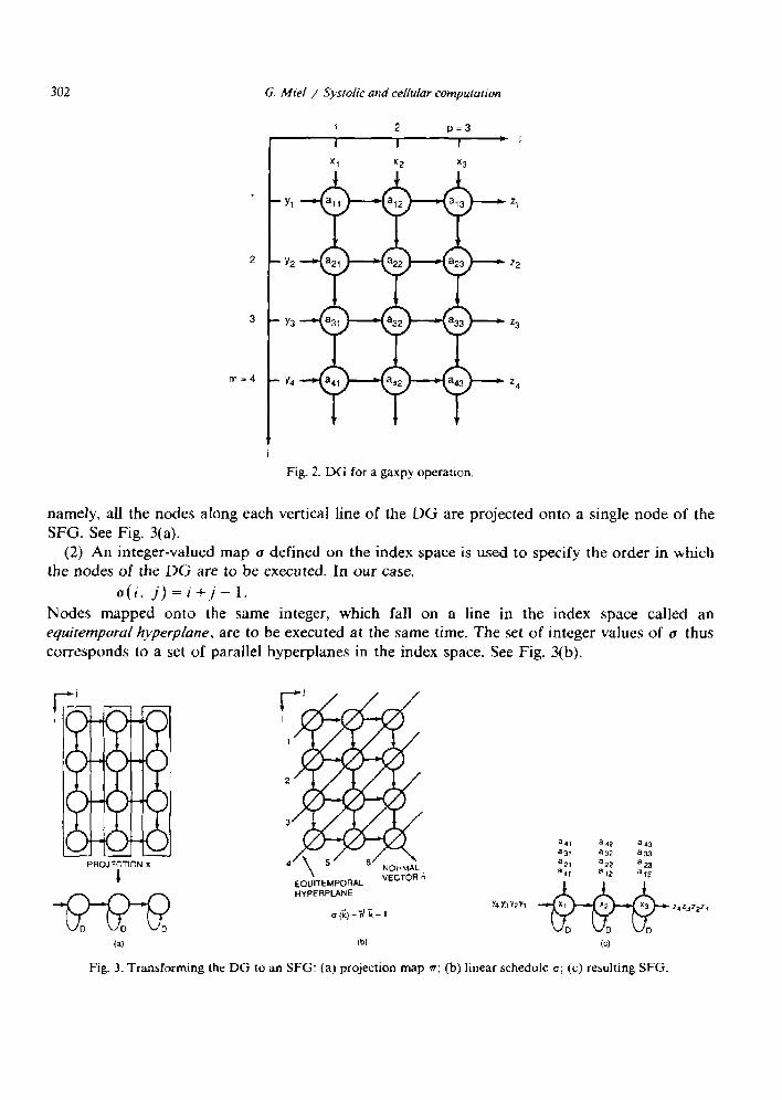
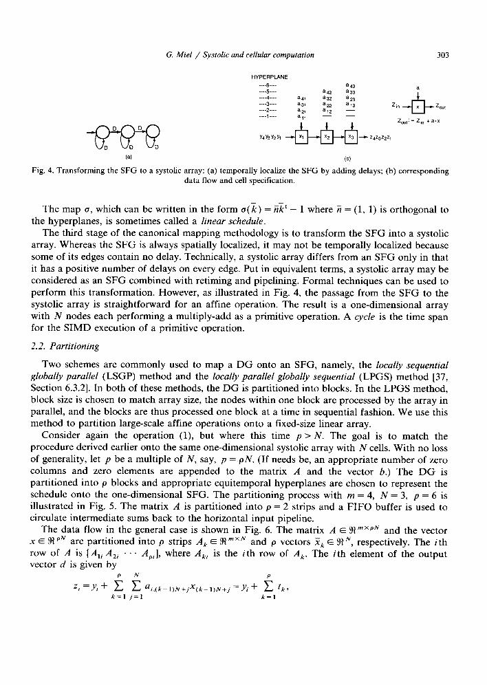
Fig. 4. Transforming the SFG to a systolic array: (a) temporally localize the SFG by adding delays; (b) corresponding data flow and cell specification.

The map u, which can be written in the form a(k) = ix’ - 1 where fi = (1, 1) is orthogonal to the hyperplanes, is sometimes called a linear schedule.

The third stage of the canonical mapping methodology is to transform the SFG into a systolic array. Whereas the SFG is always spatially localized, it may not be temporally localized because some of its edges contain no delay. Technically, a systolic array differs from an SFG only in that it has a positive number of delays on every edge. Put in equivalent terms, a systolic array may be considered as an SFG combined with retiming and pipelining. Formal techniques can be used to perform this transformation. However, as illustrated in Fig. 4, the passage from the SFG to the systolic array is straightforward for an affine operation. The result is a one-dimensional array with N nodes each performing a multiply-add as a primitive operation. A cycle is the time span for the SIMD execution of a primitive operation.

2.2. Partitioning

Two schemes are commonly used to map a DG onto an SFG, namely, the locally sequential globally parallel (LSGP) method and the local& parallel globally sequential (LPGS) method [37, Section 6.3.21. In both of these methods, the DG is partitioned into blocks. In the LPGS method, block size is chosen to match array size, the nodes within one block are processed by the array in parallel, and the blocks are thus processed one block at a time in sequential fashion. We use this method to partition large-scale affine operations onto a fixed-size linear array.

Consider again the operation (l), but where this time p > N. The goal is to match the procedure derived earlier onto the same one-dimensional systolic array with N cells. With no loss of generality, let p be a multiple of N, say, p = pN. (If needs be, an appropriate number of zero columns and zero elements are appended to the matrix A and the vector b.) The DG is partitioned into p blocks and appropriate equitemporal hyperplanes are chosen to represent the schedule onto the one-dimensional SFG. The partitioning process with m = 4, N = 3, p = 6 is illustrated in Fig. 5. The matrix A is partitioned into p = 2 strips and a FIFO buffer is used to circulate intermediate sums back to the horizontal input pipeline.

The data flow in the general case is shown in Fig. 6. The matrix A E %jmXpN and the vector x E !R pN are partitioned into p strips A, E !RTjmxN and p vectors Xk E % N, respectively. The i th row of A is [A,, A,, . . . A,,], where Aki is the ith row of A,. The ith element of the output vector d is given by

Zi=_Y, + f: 5 ai,(k-l)N+jX(k-l)N+j=_&+ i tk, k=l j=l k=l

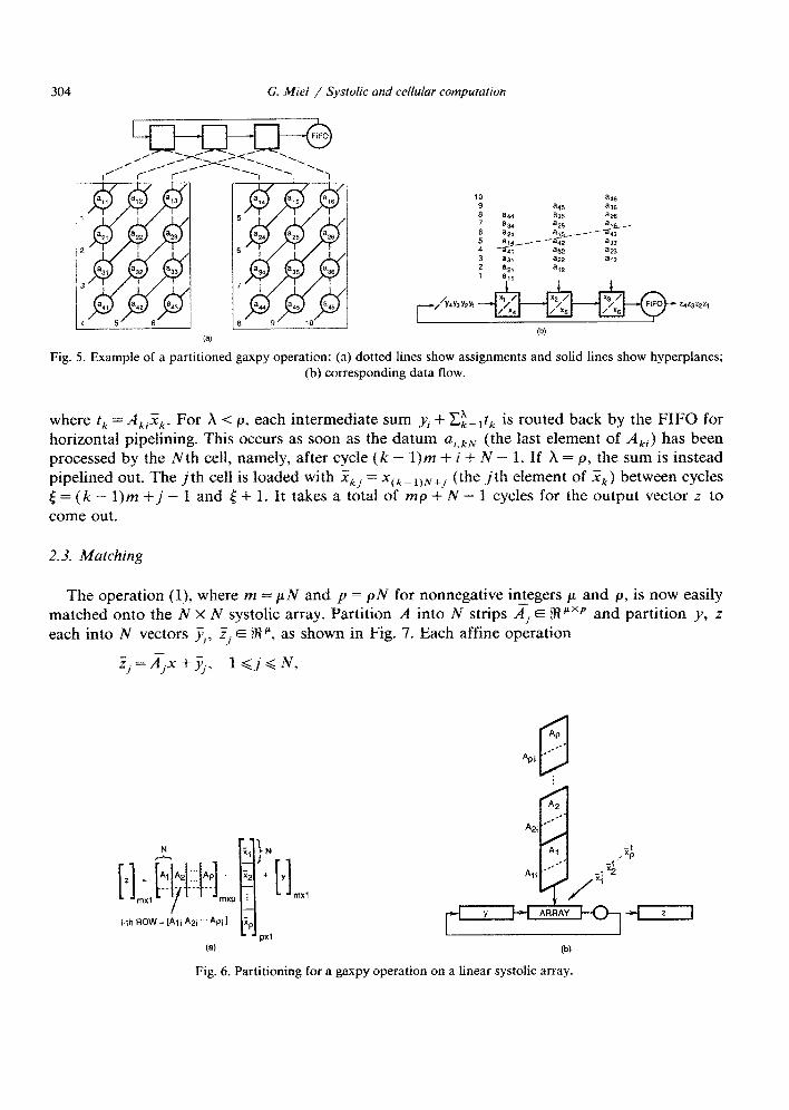
(b)

Fig. 5. Example of a partitioned gaxpy operation: (a) dotted lines show assignments and solid lines show hyperplanes;

(b) corresponding data flow.

where t, = AkiXk. For .A < p, each intermediate sum yj + Ci=,t, is routed back by the FIFO for horizontal pipelining. This occurs as soon as the datum ai,kN (the last element of Aki) has been processed by the Nth cell, namely, after cycle (k - l)m + i + N - 1. If X = p, the sum is instead pipelined out. The jth cell is loaded with Xk, = xCk_itivtj (the jth element of Xk) between cycles [ = (k - l)m +j - 1 and 5 + 1. It takes a total of mp + N - 1 cycles for the output vector z to come out.

2.3. Matching

The operation (l), where m = PN and p = pN for nonnegative int_egers J.J and p, is now easily matched onto the N X N systolic array. Partition A into N strips A,. E j9?“xp and partition y, z each into N vectors JJ,, Zj E %I’, as shown in Fig. 7. Each affine operation

3,=&x +j$ 1 <j<N,

AP a *. Api

,a--

A2

w (b)

Fig. 6. Partitioning for a gaxpy operation on a linear systolic array.


Zl

____

22

___.

____

iN

._

‘I

Al ._______________--.

A2 ._____________----. .

AN

nx1 I- - mxp

Yl

.______

72

+ _______

:

._____-

PXl YN

i mxl

;j =AjX+y’ I

1CjsN

Fig. 7. Partitioning for a gaxpy operation on a square systolic array.

is partitioned as in Section 2.2 on a row of the square array. The N rows operate in parallel. Each row has its own vertical pipeline and there is no data transfer between rows. The process requires T = pp + N - 1 cycles to produce the complete output. Ignoring costs of data movement, idealized speedup is ppN2/T compared to serial computation.

In the special case m = p = pN, a method for transforming a linear systolic array into a rectangular p x N systolic array has recently been given [49]. However, this is not a matching procedure, since the dimensions of the resulting array are problem dependent.

3. Systolic linear solvers

In this section, we describe two systolic algorithms for solving systems of linear equations. The first algorithm consists of an iterative method based on the systolized gaxpy operation described earlier. The second algorithm uses a modification of the Faddeev procedure [24,62].

3.1. Iterative method

Given a matrix L = J - K E 8 nxn, where J is invertible, and a system Lu = v. If M = J-‘K has a spectral radius less than one, then x,,, the Neumann iterates

x, = Mx,_, + w, w = J-b,

converge to u = L-b. Moreover, if ]I J-’ 11 11 K II G j3 c 1, then

II u - x, II G &II X,--xgll-

When the matrix M is dense and large, the iteration (3) is rarely used to its linear convergence.

because it is costly relative

A little-known modification due to [50], which yields quadratically convergent iterates, is advantageously implementable on square systolic arrays. The Hotelling-Lonseth iterates y, are

vector v E !lI “, consider a L is invertible and, for any

(3)

306 G. Mel / SystoIic and cellular computation

defined by the double recurrence

Yo =x0, zo= w,

y, = M*‘-‘y;_, + Z,_l, z, = M*‘-‘Z,_l + z,_l. (4)

It turns out that y, = x2’_i. If y. = w, then z, =y,. and the iterates y, are obtained from a single recurrence relation.

After initialization of M and y, the first R iterates (4) are obtained as follows:

For r = 1, 2,. . . , R y: =My+z z:=Mz+z M:=MM End

When r = R, the second gaxpy and the matrix multiplication need not be done. Hence, the procedure takes (2 R - 1)To + (R - l)T, cycles for arbitrary y. and RT, + (R - l)T, cycles if y, = w, where TG, TM are respectively the cycle counts for a gaxpy operation and a matrix-matrix multiplication.

Assume that the algorithm is executed on an N X N square mesh array processor and that n = vN, where v is a positive integer. From Section 2.3, we find that TG = v* + N - 1. Each column of the matrix product MM can be computed as a gaxpy operation partitioned as described in Section 2.2 on a single row of the array processor, with the N rows working in unison. We thus get that TM = ( v3 + 2v) N - 2v, referring to [57] for details.

The Neumann iteration (3) for computing y, on the same systolic array takes (2R - 1)To cycles. Thus the general Hotelling-Lonseth iteration has smaller arithmetic complexity on the systolic array only if the number of iterates R satisfies

For example, on a 16 x 16 systolic array, this is the case for a 128 x 128 linear system if R 2 10, whereas on a 128 X 128 systolic array it is so for any R >, 1.

We emphasize that the cycle counts refer only to numbers of scalar multiply-add operations executed in SIMD mode. For simplicity, we have ignored the cost of data management. In practice, however, data formatting and partitioning become increasingly costly when the dimension of the problem gets larger than the dimension of the systolic array.

3.2. Modified Faddeev method

Consider four matrices A, tableau:

n 4

AIB m

_CP in which the letters m, n, p, q denote dimensions of the matrices. Suppose that m = n and that

B, C, D arranged for convenience as shown in the following

G. Mel / Systolic and cellular computation 307

A is invertible. The Faddeeu algorithm [24] uses Gaussian elimination to annul the lower left-hand quadrant of the tableau. Namely, multiples of rows of the upper part [A, B] are systematically added to rows of the lower part [ - C, D] until - C is replaced by the p x n zero matrix. Assuming that there is no zero pivot, the Schur complement

CA-‘B+ D

will then replace D in the lower right-hand quadrant. Note that a matrix multiply-add can be executed by taking A = I and that a gaxpy operation is obtained by further taking q = 1. The case with C = I, D = 0 solves the matrix equation AX = B.

In contrast to the LU or QR factorization method, the Faddeev algorithm avoids the backsubstitution step used in solving an upper triangular system. This feature greatly facilitates mapping of the algorithm onto an array processor. On the other hand, partial or full pivoting, needed to avoid zero pivots and to control roundoff, is costly to implement on an array processor with nearest-neighbor connectivity. Furthermore, the direct application of orthogonal transformations to annul - C results in a modification of the Schur complement.

In order to circumvent these problems, Nash and Hansen [62] proposed a modification of the Faddeev algorithm based on both orthogonal transformation and Gaussian elimination. Con- sider again the tableau, this time with m > n, and assume that A has rank n. The modified algorithm proceeds in two stages.

Stage 1. The matrix A is triangularized using Givens rotations to get

n 4

R []I[ 1 0 Q:, n

Q: m-n

-cl D P

where Q = [Q,, Q2] is the orthogonal factor in the QR factorization of A.

Stage 2. Gaussian elimination is then applied to annul - C, using the diagonal elements of R as pivots, to get

n 4

R [III 1 0 QiB n

Q: m-n

0 /CR-‘Q;B+D p

Since A is assumed to have full rank, the diagonal elements of R are nonzero, and thus division by zero in the second stage is theoretically impossible. For any one column b of B, the vector R-‘Qib is the least-squares solution to the overdetermined system Ax = b.

We see that the modified Faddeev algorithm consists of an orthogonal transformation of A extended to B, followed by Gaussian elimination of -C with corresponding row operations extended to D. Rearrangements of the tableau provide for the solution of underdetermined and generalized least-squares problems [62].

308 G. Miel / Systolic and cellular computation

x. In

(5 ‘ W)

BOUNDARY CELL:

b44

b43 44 b 42

b 33

b 24

b 41 b 32 b23

b 14

b a44 31 b22 bl3

a43 a34 b21 bl2

a42 a33 a24 all

a41 a32 a23 74

a31 a22 a13

a21 52

%,

(a)

INTERNAL CELL:

x Out

=-sr+cx. In

r=cr+sxin

c>- r XolJt Y r Y

+b

xout BOUNDARY CELL:

/r

INTERNAL CELL: X =x. out I" Xout=Xin-Yr

IF x in=O, r=OTHEN

c=l s=o

ELSE t={m

c = r/t

s = x in/t

X. In X.

I"

r=t

(W (c)

Fig. 8. Modified Faddeev method: (a) trapezoidal-array processor; (b) cell specification for rotation stage; (c) cell specification for elimination stage.

From the point of view of algorithmic mapping, the main advantage of the modified Faddeev algorithm is that both its stages can be mapped onto the same systolic array. As illustrated in Fig. 8(a), this array has trapezoidal shape and mesh connectivity. The circles and squares denote respectively boundary and internal processing cells. Cell specifications for the two stages are indicated in Figs. 8(b) and 8(c), respectively. In Stage 1, the boundary cells compute sines and cosines of Givens rotations while internal cells perform the rotations. In Stage 2, boundary cells


L-J L-J L--IL-J L-J L-J L-J y y,,y-l .y, t-17 -II- -lr

Fig. 9. Square array for modified Faddeev method

compute multipliers while internal cells perform the eliminations. In the Givens rotation stage, a skewed alignment of the matrices A and B is pipelined vertically through the array processor, with A and B respectively passing through the triangular and rectangular part of the trapezoid. Simultaneously, sines and cosines generated by the boundary processors are pipelined horizontally through the entire array. Data movement during the Gaussian elimination stage is analogous, with the matrices C and D pipelined vertically and the multipliers pipelined horizontally.

The trapezoidal systolic array of Fig. S(a) is readily transformed into the square structure shown in Fig. 9. These figures illustrate the case when A and B are both 4 x 4 matrices. In the square-array processor, the data flows south until it reaches the main diagonal, then it moves west to a certain subdiagonal, determined by the size of the problem, and then moves south again to exit the array. Computations occur in the horizontal phase of the flow, while the processors on the vertical path provide time delays.

Partitioning techniques exist when the problem size exceeds that of the array processor. One such technique consists of dividing the block matrices [A, B] and [ - C, D] into vertical strips of width equal to that of the array. Each strip is further divided into blocks matching the size of the array. The processing proceeds in several steps, with each step operating on all corresponding blocks of the strips. In any one step, the boundary cells generate their elements using data in the left-most strip, and during the remainder of the step, the internal cells use these elements for rotations or eliminations on the remaining data. We refer to [62] for details.

4. Cellular fast Fourier transform

The algorithms that we have described so far are of systolic type. During their execution, the cells in the array processor regularly pump data in and out, each time performing simultaneously a short computation, with the data systematically pipelined through the network. This mode of


operation requires that the algorithms be homogeneous and locally repetitive, as exemplified by the linear-algebraic operations that we considered.

In the cellular mode, the input data are first loaded into the array, then processed in unison using as many steps as needed, including possible intercellular data transfers, and the results are then unloaded from the array. There is no orderly pipelining as in the systolic mode, and consequently, computation and data movement usually cannot be balanced for optimal concur- rency. Hence, the cellular mode is generally not as efficient as the systolic mode. However, procedures that cannot be systolized must then be mapped in cellular mode. Fast Fourier transforms (FFTs), which have an inherently global data dependency that hinders local communication, are among such procedures.

We illustrate the cellular mode by describing a recent FFT algorithm for rectangular array processors [56]. The FFT is said to have constant geometry because the communication pattern shown in its dependence graph is periodic, namely, the addressing of operands for the arithmetic operations is the same from stage to stage. Such FFTs were originally derived by Pease [69], using matrix factorizations to modify and parallelize the usual Cooley-Tukey procedure. For the N-point radix 2 case, the algorithm consists of log,N stages each preceded by a perfect shuffle of the data. The most natural mapping of this algorithm is onto a linear-array architecture with +N cells and a shuffle-exchange interconnection network [82,84].

Our strategy is to further decompose the Pease factorization in order to map a 2MNs-point radix 2 FFT onto an M X N rectangular array processor. The result depends fundamentally on a factorization of the perfect-shuffle permutation. The corresponding data movement is realized in parallel as relatively small perfect shuffles inside each local memory and along each row and column of the array processor, without requiring that the complete array itself have the shuffle-exchange interconnection network. While matrix operations were heretofore the objects of our algorithms, in this section we additionally use linear algebra to validate the actual mapping of the algorithm to the architecture.

4.1. Matrix factorizations

A perfect shuffle is a permutation that transforms the 2m-vector

z= (0, l,..., m-l, m, m+l,..., 2m-1)’

to the vector

SZmz=(O, m,l, m+l,..., i, m+i ,..., m-1,2m-1)‘. (5)

Components that were m apart become adjacent as a result of .the perfect shuffle. For convenience, we simply call (5) the shuffle of z.

A standard result in algebra provides a constructive method for factoring any permutation as a product of 2-cycles, e.g., [30, p.781. Moreover, any 2-cycle is itself a product of 2-cycles involving only adjacent components. Hence, letting (k) denote the exchange of the k th and (k + 1)th components, one can show that

S,, = T,_, . . . T,T,, (6)

where q is a product of i adjacent exchanges:

q=(m-i)(m-i+2)**+(m+i-2).


The case for m = 4 is shown below:

T, = (3): 01 2 3-4 5 6 7 T, = (2)(4): 0 1 2-4 3-5 6 7 T3 = (l)(3)(5): 0 1 ++ 4 2-5 3-6 7 s,: 04 1 5 2 6 37

Since the i exchanges in q. are independent of one another, they can be done in parallel. A consequence is that the factorization (6) can be implemented on an array processor with nearest-neighbor connectivity in m - 1 steps, with the jth step consisting of the parallel execution of the i exchanges in 7].

The following factorization of the shuffle permutation has a basic role in our presentation.

Proof. We show that the effect of the factorization on the vector z = (0, 1,. . . ,2KL - 1)’ is the vector

(0, KL,l, KL+l,..., j, KL+j ,..., KL-1,2KL-1)‘.

Partition z into 2 K L-tuples,

Z = (E,, z,, . . . , &_J,

where

(7)

E,=(iL, iL+l,..., iL+j ,..., (i+l)L-1).

We find that

(I, @ S*,)z = ( zO, z,,. .., Z,, ZK+r,. . . , &, z,,_,)‘.

The effect of applying S,, @ IK on this vector is that of replacing the 2 L-tuple ( Zj, Z,, ;) by

MC, &+,Y

=S,,(iL ,..., iL+j ,..., (i+l)L-l,(K+i)L ,..., (K+i)L+j ,...,

(K+i+l)L-1)’

=(iL, iL+KL ,..., iL+j, iL+j+KL ,..., (i+l)L-l,(i+l)L-l+KL)‘.

The concatenation for i = 0, 1,. . . , K - 1 of these 2 L-tuples yields the desired vector (7). III

The factorization in the lemma is analogous to cutting a deck of 2KL cards into a row of 2K subdecks of L cards each, rearranging these subdecks according to the shuffle permutation, shuffling together adjacent pairs of subdecks, and then collecting the resulting K subdecks into a single deck.

The discrete Fourier transform of a complex P-vector z = ( zO, zr, . . . , z~_~)~ is Fz, where F is a complex P x P matrix whose (A, p)th element is &‘, 0 < X, I_L < P - 1, where w = eCiZn/’ and i2 = - 1. The Pease factorization [69] of the matrix F can be expressed as

UF= (A’P-?Sp) ... (A”‘S,&4’“‘Sp), (8)

(9)

The k th stage of this FFT is represented by nlkjSp. where k = 0, 1, _. . . p - 1 and p = log,P. The matrix C’ is the permutation matrix that represents the bit-reversed order of the output vector. Each 2 x 2 matrix B(m). applied on a pair of adjacent data, is called a hutterf(rl operation. The element u”’ is called a rGd& Jacror. For our purposes here, we need not define the exponents c(‘). The usual parallel implementation of (8) is on a linear array processor with +P cells, with &ch cell containing a pair of adjacent data. Each stage of the FFT begins with a perfect shuffle, involving data transfers among the cells, followed by a SIMD butterfly operation.

The following theorem, which further decomposes the Pease factorization, engenders a parallel FFT algorithm for an M x IV rectangular array processor.

The desired result follows. 0

04)

4.2. Basic algorithm

Let P = 2M~s where M. N. s are powers of 2 with nonnegative integer exponents. Our goal is to describe a parallel FFT algorithm for a 2-dimensional M x hi array processor. We first specify needed features of the targeted architecture.

Storage. Each of the MN cells has a local memory with 2s locations, each able to contain a complex datum, denoted by R,: R,, . . . 1 R ?$_ 1. A complex P-vector z is stored so that pairs of


m=O

Qi

I

Ri+s

(a) (b)

m=3 Fl & (4

Fig. 10. Connectivity when M = N = s = 4; (a) rshuffle in one, cell; (b) xshuffle(i) in one row; (c) yshuffle(i) in one column.

locations R,;, Rzi+, contain adjacent data z,,, z~,+~. The symbol R~“‘~“’ denotes the content of the ith location in the (m,n)th cell of the array processor. The 2s-vector

R’ m.n) - - ( Rbm5”‘, Rim3”‘, . . . , R;;:“?)’ (15)

represents the data in the local memory of the (m, n)th cell.

Communication. In addition to (15), consider the vectors

X’“’ = (R$;,“, R$;;‘;, R;~~“, R$‘$;, . . . , R$y+‘), R(211;7-‘) )‘T

y(“, = (RIO.“), RIO;;‘, @s”), R;>;), . . . , R;“-lTJ), R;y;ld)t. I

We assume that the array processor can execute the following three operations: rshuffle: replace R’“+) by S,,yR’“s”’ simultaneously for m = 0, 1,. . . , A4 - 1 and n =

0, I..., N- 1; xshuffle( i): for fixed i, replace X/“’ by S,, X!“’ simultaneously for m = 0, 1,. . . , M - 1; yshuffle( i): for fixed i, replace KC’) by SZMy(“) simultaneously for n = 0, 1,. . . , N - 1.

The rshuffle operation consists of MN parallel shuffles of the 2s memory locations in each cell. This operation does not involve data transfers among cells, unlike the other two operations. The xshuffle(i) operation consists of M parallel shuffles, one in each row of the array, involving the pair of locations Rzi, R2,+, in each cell. The yshuffle(i) operation consists of N parallel shuffles, one in each column of the array, involving the pair of locations R;, R,+s in each cell. The connectivity in these operations is illustrated in Fig. 10 for the case M = N = s = 4.

Arithmetic. For fixed i and k, let arith( k, i) denote the parallel butterfly operation that replaces 2, = ( R2;, Rzj+l)’ in each cell by B( X)R,, where B(X) is the 2 x 2 matrix defined in (9) and X is an appropriate exponent. The totality of ;P butterflies in the k th stage of the FFT is obtained by executing arith( k, 0), arith( k, l), . . . ,arith( k, s - 1).

The desired algorithm is a transliteration of the factorization (10). The correspondence between the contents of the local memories and a P-vector z is given by the bijection

@:z-+ { Rjr”,“’ } SE 2,

( R$y3”‘, R:Y?) = (z+,, z++l ), +=+(i, m, n)=2N(i+ms)+2n. (16)

314 G. Mel / Systolic and cellular computation

The effect of C, is to perform a shuffle on every 2N-tuple in z and the application of @ after this permutation results in a natural ordering of the data in the local memories. Since both the input and output vectors in (10) are premultiplied by the matrix C,, the mapping

\k:z+.GJ?, *z = @C,z,

m.n) - RI -z+, $=$(i, m, n)=(i+2ms)N+n,

defines the correspondence between the P-vector and the local memories, respectively during the loading at the start and the unloading at the end of the FFT. During the FFT itself the correspondence is given by @. The natural ordering induced by 4 facilitates loading and unloading and it is useful for bit-reversed sorting of the output.

It can be shown formally [56] that the operation rshuffle carries out the permutation C,, that the collective effect of the s operations

yshuffle(O), yshuffle(l), . . . , yshuffle( s - 1)

is that of the permutation C,, and likewise, that the s operations

xshuffle(O), xshuffle( 1)). . . , xshuffle( s - 1)

represent the permutation C,. Consequently the factorization (10) in Theorem 2 yields the following algorithm for executing

a P-point FFT on the M x N array processor:

Load \kz For k=O, l,...,p-1

For i=O, l,...,s- 1 yshuffle( i)

rshuffle For i = 0, 1,. . . , s - 1

arith( k, i) For i = 0, 1, _ . . , s - 1

xshuffle( i) Unload \k-‘UFt

The For-k loop represents the p = log,P stages of the FFT. The unload operation usually includes a bit-reversed sort to get Fz in natural order. For the special cases M = s = 1 or N = s = 1, the above algorithm becomes the well-known Pease procedure for a linear array processor [69]. Thus, in its generality, the algorithm may be viewed as a partitioning of the Pease procedure for rectangular array processors.

4.3. Remarks

The communication complexity of the cellular algorithm for a P-point constant geometry FFT on a rectangular A4 x N array processor is dependent on the array’s ability to perform the rshuffle, xshuffle, yshuffle operations. In the ideal case, shuffle-exchange links in each local memory, row and column minimize the cost of data movement. In the case of an N X N array processor with square mesh connectivity, the shuffles become costly for large N. Thus, for an FFT with P = 2N2s points, using the factorization (6) of the perfect shuffle as a product of


adjacent exchanges, if we assume that North-South and East-West intercellular exchanges and internal register exchanges each have unit cost, we find that the communication complexity is

(2N.s - s - 1)(2 log,N + log,s + 1).

On the other hand, it is

6 log,N + 3 log,s + 3

in the idealized case for an N X N array processor having maximally redundant shuffle-exchange links each with unit cost.

In addition to constant geometry FFTs, the perfect shuffle has wide applicability in parallel processing, including bitonic sorting, polynomial evaluation, matrix transposition, and linear transformations [5,21,82,84]. Hence, implementations of the perfect shuffle engendered by matrix factorizations (14) for rectangular array processors, or extensions for higher-dimensional arrays, can be put to good usage for such applications. Moreover, assuming bidirectional links in the shuffle connections, we have access to the inverse perfect shuffle for the class of algorithms based on recursive doubling [36,83]. In this case, a factorization corresponding to that in the lemma,

serves as the basis for deriving representations of the inverse perfect shuffles on array processors. The lemma and the theorem extend to radix r constant geometry FFTs for d-dimensional

array processors [56]. The matrix factorization corresponding to an FFT is then obtained by d applications of a basic factorization of the radix r shuffle permutation extending that of the lemma for the radix 2 case. The resulting data movement involves parallel radix r shuffles in each local memory and along each of the d-dimensional axes of the array processor. The data is loaded in natural order and each cell performs a butterfly by operating on r consecutive registers Ri> Ri+r,*. .T Ri+,-le

5. Active research areas

Due to space constraints, we are unable to describe numerous aspects of systolic and cellular computation. Our goal in this section is to provide snapshots, using annotated lists of recent references, of current research activities on the topic.

5.1. Systems of linear equations

The Gauss-Jordan method for matrix inversion, when compared to triangular matrix factorization techniques, performs poorly on serial computers. However, with no row or column interchange, it parallelizes remarkably well on array processors. Moreover, the method then embodies abstract recurrence relations solving the so-called algebraic-path problem, which encompasses as special cases, in addition to matrix inversion, the transitive closure and shortest-path problems in graph theory and regularization of languages in automata theory, see [28]. Descriptions of systolic arrays for the solution of the algebraic-path problem can be found in [48]. Such systolization illustrates nicely the symbiosis between mathematical structure and, at the conceptual level, array architecture.

316 G. Miel / Systolic and celhlar computation

Systolic arrays for LU and QR factorizations of matrices have been known since the early 1980s see [26,46]. Partial or full pivoting, needed to avoid zero pivots and to control roundoff, is not readily amenable to parallel computation on array processors with nearest-neighbor connectivity. Gentleman and Kung [26] used so-called neighbor piuoting, in which the pivot is selected as the largest element among neighbors, to devise a systolic array for matrix triangularization. Roychowdhurry and Kailath [76] have presented a systolic array for LU factorization with partial pivoting, with the property that the rows of the resulting upper triangular factor are not naturally ordered, thus necessitating considerable overhead in the determination of the solution vector. Cholesky factorization LL’, via the use of hyperbolic transformations, has been mapped onto a systolic array in [15].

The systolized version of the modified Faddeev method, described in Section 3.2, dates back to the mid 1980s see [61,62]. The Faddeev algorithm was also systolized in [12] for both fixed-size and variable-size problems, and in [14] for partitioned implementation on two-dimensional arrays of transputers. Moreno and Lang [59,60] used their mapping technique, the so-called multimesh graph method, to partition the Nash-Hansen procedure onto both l-dimensional and 2-dimensional systolic arrays. With the hypothesis that there be no data duplication, it is widely believed, though apparently no one has proved it, that optimal complexity for inversion of a dense n X n matrix on a systolic array is 5n inner product steps. The Nash-Hansen version of the Faddeev method and other systolic matrix inverters reach this bound. Megson [54] has recently proposed a Faddeev array that achieves matrix inversion in just 4n steps with O(n2) basic cells using careful duplication of some data.

Deprettere and Jainandunsing [17,31-331 have analyzed a class of systolic algorithms, called feed forward methods, for solving nonsingular systems. The solution of Ax = b is obtained through a combination of an LU, LQ or LL’ factorization of A and, if L denotes the respective lower triangular factor, an updating or downdating of the Cholesky factorization of LL’ + bb’ or LL’ - bb’, respectively, or an LU factorization of [L, - b’]*. Like the Faddeev algorithm, the feed forward methods avoid backsubstitution and they can be generalized to compute Schur complements.

5.2. Singular-value decomposition

The singular-ualue decomposition (SVD) of a matrix provides the most efficient computational method for the determination of the rank of a matrix, it yields the best approximation in a least-squares sense of a high-dimensional matrix by a lower-dimensional one, and it provides the most numerically stable solution to least-squares estimation problems, see [27].

Because of such properties, there has been considerable interest on the use of SVD techniques in digital image and signal processing. For example, it has been known for a long time that the SVD is useful in image enhancement, moving target tracking, harmonic retrieval problems and image reconstruction. Refer respectively to [3,4,38,78]. Continuing research aims to find high-res- olution algorithms for extracting signal and system parameters from measurements, using the SVD of appropriate data matrices as a means for robust separation of signal and noise, see

[6,161. For real-time or high-throughput applications, such as in avionics and space systems, systolic

and cellular array processors provide a modern and attractive approach to computing the SVD of given matrices. Pertinent algorithms, for the SVD and related decompositions, have been


presented in [7,8,22,23,51-53,851. Comon and Golub [13] have recently analyzed various numeri- cal methods for finding extreme singular values and corresponding left singular vectors when the matrix is slowly varying in time. Such algorithms are of crucial importance in signal-processing applications based on low-rank approximation of a time-dependent covariance matrix, see the references cited in [13].

5.3. Artificial neural networks

There is extensive ongoing research on neural networks and their representations on array processors. An introductory description of the subject can be found in [37, Section 4.61. Recent texts on the topic are [20,79,80]. Applications in neural computing include combinatorial optimization, image and signal processing, artificial intelligence, etc. An early systolic architecture for an artificial neural network was designed in [39]. The same authors recently proposed [40] a unified architecture, consisting of a programmable ring systolic array, that provides for both the retrieving and the learning phases of a wide variety of artificial neural networks. A concise taxonomy of artificial neural networks is given in the introduction of that article.

Przytula et al. [70] have described graph-theoretic techniques for implementation of a wide class of neural networks of arbitrary size on mesh-connected SIMD arrays of fixed size. Shams and Przytula [77] used a multilayer perception network, implementable on 2-dimensional array processors, for underwater target detection. Other applications of artificial neural network in signal processing are described in references cited in [70]. A quick overview of other current activities on neural computing, e.g., on theory and algorithms, speech and image processing, and on implementation methods, can be gleaned from the proceedings [2] of a recent EURASIP workshop.

5.4. Simulated annealing algorithm

Simulated annealing, so called because of its conceptual analogy with metallurgical annealing, uses a stochastic approach to combinatorial optimization. The algorithm has diverse applications in job shop scheduling, circuit design, artificial intelligence, image restoration, etc. See, e.g., [29,44,45]. A general-purpose optimization routine, based on the annealing algorithm and written in Pascal, was published in [68]. A design for a simulated annealing array processor was presented in [37, Chapter 81, [41].

We make special mention of simulated annealing because the algorithm is closely related to Boltzmann machines, see [l], and because the latter topic provides a rigorous mathematical base from which to penetrate the much less rigorous, but quickly emerging, area of neural computing. A Boltzmann machine is a network of elements, each with state either 0 or 1, bidirectionally interconnected with strengths that can take arbitrary values. The aim is to maximize a consensus function C, defined as the sum of products of corresponding states and strengths. A transition unit is chosen for proposed changes in the machine. Such a change is accepted if either C increases or if l/(1 + e- Ac’s) is less than a uniformly distributed random number in [0, 11. A decreasing sequence of s values, called a cooling schedule, is used to bring the Boltzman machine into near optimal configuration.

Since the appearance of papers by Kirkpatrick et al. [35] in 1982 and Cerny [ll] in 1985, who initiated the research on the subject, the analytical framework behind simulated annealing has


considerably evolved. There is an extensive body of knowledge on global convergence properties of the simulated annealing algorithm. Since Boltzmann machines are analogous to simulated annealing, there are predictably corresponding results for Boltzmann machines. However, if in the definition of the Boltzmann machine one allows the choice of transition units to be implementable in parallel, asymptotic convergence for the resulting network appears to be still an open problem.

Acknowledgements

The author is grateful to colleagues at Hughes Research Laboratories, Greg Nash, Wojtek Przytula and David Schwartz, who provided much of the information contained in this paper.

References

[l] E. Aarts and J. Korst, Simulated Annealing and Boltzmann Machines (Wiley/Interscience, New York, 1989). [2] L.B. Almeida and C.J. Wellekens, Eds., Proceedings of Neural Networks, E URASIP Workshop 1990, Sesimbra,

Portugal, 1990, Lecture Notes in Comput. Sci. (Springer, Berlin, 1990). [3] H.C. Andrew and C.L. Patterson, Singular value decompositions and digital image processing, IEEE Trans.

Acoust. Speech Signal Process. (1976) 26-53. [4] I.L. Ayala et al., Moving target tracking using symbolic registration, IEEE Trans. Pattern Anal. Mach. Intell.

(1982) 515-520. [5] K.E. Batcher, Sorting networks and their applications, in: 1968 Spring Joint Computer Con&, AFIPS Proc. 32

(Thompson, Washington, DC, 1968) 307-314. (61 E. Biglieri and Yao, Some properties of singular value decomposition and their applications to digital signal

processing, Signal Process. 18 (1989) 277-289. [7] R.P. Brent and F.T. Luk, The solution of singular-value and symmetric eigenvalue problems on multiprocessor

arrays, SIAM J. Sci. Statist. Comput. 6 (1985) 69-84. (81 R.P. Brent and F.T. Luk, Computation of the singular value decomposition using mesh-connected processors, J.

VLSI Comput. Systems 1 (1985) 243-270. [9] P.R. Cape110 and K. Steiglitz, Unifying VLSI array design with geometric transformations, in: Proc. I983

Znternat. Conf: on Parallel Processing (1983) 448-456. [lo] P.R. Cape110 and K. Steiglitz, Unifying VLSI array design with linear transformations of space-time, Adu. in

Comput. Res. 2 (1984). [ll] V. Cerny, Thermodynamical approach to the traveling salesman problem: An efficient simulation algorithm, J.

Optim. Theory App{ 45 (1985) 41-51. [12] H.Y.H. Chuang and G. He, A versatile systolic array for matrix computations, in: 12th Annual Symp. on

Computer Architectures (1985) 315-322. [13] P. Comon and G.H. Golub, Tracking a few extreme singular values and vectors in signal processing, Proc. IEEE

78 (1990) 1327-1343. [14] A.J. de Groot, E.M. Johansson and S.R. Parker, Systolic array for efficient execution of the Faddeev algorithm,

in: Proc. SPIE, Real-Time Signal Processing X (1987) 86-93. [15] J.-M. Delosme and I.C.F. Ipsen, Efficient systolic arrays for the solution of Toeplitz systems: an illustration of a

methodology for the construction of systolic architectures in VLSI, in: Proc. Znternat. Workshop on Systolic Arrays (1986) F3.1-F3.22.

[16] E.F. Deprettere, Ed., Singular Value Decomposition and Signal Processing. Algorithms, Applications and Architec- tures (North-Holland, Amsterdam, 1988).

[17] E.F. Deprettere and K. Jainandunsing, Orthogonal and J-orthogonal matrix inversion techniques, in: Proc. ISCAS (1987).


[18] J.J. Dongarra, Performance of various computers using standard linear equations software in a Fortran

environment, Technical Memorandum 23, Math. Comput. Sci. Div., Argonne National Laboratory, 1987.

[19] J.J. Dongarra, J.L. Martin and J. Worlton, Computer benchmarking: paths and pitfalls, IEEE Spectrum (1987)

38-43. [20] R. Eckmiller and C. v.d. Malsbury, Neural Computers, NATO Adv. Sci. Inst. Ser. F: Comput. Systems Sci.

(Springer, New York, 1988). [21] T. Etzion and A. Lempel, An efficient algorithm for generating linear transformations in a shuffle-exchange

network, SIAM J. Comput. 15 (1986) 216-222. [22] L.M. Ewerbring and F.T. Luk, Computing the singular value decomposition on the Connection Machine, in: E.F.

Deprettere, Ed., Singular Value Decomposition and Signal Processing. Algorithms, Applications and Architectures

(North-Holland, Amsterdam, 1988) 407-424. [23] L.M. Ewerbring and F.T. Luk, Canonical correlations and generalized SVD: applications and new algorithms, J.

Comput. Appl. Math. 27 (l&2) (1989) 37-52. [24] V.N. Faddeeva, Computational Methods of Linear Algebra (Dover, New York, 1959) (translated by C.D. Benster). [25] K.A. Gallivan, R.J. Plemmons and A.H. Sameh, Parallel algorithms for dense linear algebra computations, SIAM

Rev. 32 (1990) 54-135.

[26] M.W. Gentleman and H.T. Kung, Matrix triangularization by systolic arrays, in: Proc. SPIE, Real-Time Signal Processing IV (1981) 19-26.

[27] G.H. Golub and C.F. Van Loan, Matrix Computations (Johns Hopkins Univ. Press, Baltimore, MD, 2nd ed., 1989).

[28] M. Gondran, M. Minoux and S. Vajda, Graphs and Algorithms (Wiley, New York, 1984). [29] B. Hajek, A tutorial survey of theory and applications of simulated annealing, in: Proc. 24th Conf. on Decision

and Control (1985) 755-760.

[30] I.N. Herstein, Topics in Algebra (Wiley, New York, 1975). [31] K. Jainandunsing, Parallel algorithms for solving systems of linear equations and their mapping on systolic

arrays, Ph.D. Dissertation, Delft Univ. Technology, Netherlands, 1989. [32] K. Jainandunsing and E.F. Deprettere, A novel VLSI system of equations solver for real-time signal processing,

in: Proc. SPIE, Real-Time Signal Processing IX (1986).

[33] K. Jainandunsing and E.F. Deprettere, Design of a concurrent computer for solving systems of linear equations, Comput. Architecture News 16 (2) (1988) 204-211.

[34] D.R. Kincaid and L.J. Hayes, Eds., Iterative Methods for Large Linear Systems (Academic Press, San Diego, 1990).

[35] S. Kirkpatrick, C.D. Gelatt Jr and M.P. Vecchi, Optimization by simulated annealing, IBM Research Report RC 9355, IBM Corporation, Armonk, NY, 1982.

[36] P. Kogge and H. Stone, A parallel algorithm for the efficient solution of a general class of recurrence equations, IEEE Trans. Comput. 22 (1973) 786-793.

[37] S.Y. Kung, VLSI Array Processors (Prentice-Hall, Englewood Cliffs, NJ, 1988). [38] S.Y. Kung, K.S. Arun and D.V.B. Rao, State space and SVD based approximation methods for the harmonic

retrieval problem, J. Opt. Sot. Amer. A 73 (1983) 1799-1811. [39] S.Y. Kung and J.N. Hwang, Systolic design of electronic neural networks, in: Proc. 26th ZEEE Conf. on Decision

and Control, Los Angeles, 1987. [40] S.Y. Kung and J.N. Hwang, A unified systolic architecture for artificial neural networks, J. Parallel Distrib.

Comput. 6 (1989) 358-387.

[41] S.Y. Kung, J.N. Hwang and S.C. Lo, Mapping digital signal processing algorithms onto VLSI systolic/wavefront arrays, in: Proc. 12th Annual Asilomar Conf: on Signals, Systems and Computers (1986) 6-12.

[42] H.T. Kung and C.E. Leiserson, Systolic arrays (for VLSI), in: I.S. Duff and G.W. Stewart, Eds., Sparse Matrix Proceedings 1978 (SIAM, Philadelphia, PA, 1979) 256-282.

[43] S.Y. Kung, H.T. Whitehouse and T. Kailath, VLSI and Modern Signal Processing (Prentice-Hall, Englewood Cliffs, NJ, 1988).

[44] P.J.M. Laarhoven, Theoretical and computational aspects of simulated annealing, Mathematisch Centrum, Amsterdam, 1988.

[45] P.J.M. Laarhoven and E. Aarts, Simulated Annealing: Theory and Applications (Reidel, Dordrecht, 1987). [46] C.E. Leiserson, Area-efficient VLSI computation, Ph.D. Dissertation, Carnegie-Mellon Univ., Pittsburgh, PA,

1981.


[47] C.E. Leiserson, F.M. Rose and J.B. Saxe, Optimizing synchronous circuitry by retiming, in: Proc. 3rd Caltech Conf on VLSI (1983).

(481 P.S. Lewis and S.Y. Kung, Dependence graph based design of systolic arrays for the Algebraic Path Problem, in: Proc. 12th Annual Asilomar Conf on Signals, Systems and Computers (1986).

[49] N. Ling and M. Bayoumi, Systematic algorithm mapping for multidimensional systolic array, J. Parallel Distrib. Comput. 7 (1989) 368-382.

[50] A.T. Lonseth, An extension of an algorithm by Hotelling, in: Proc. Berkeley Symp. on Mathematical Statistics and Probability 1945-1946 (Univ. of California Press, Berkeley, CA, 1949) 353-357.

[Sl] F.T. Luk, A parallel algorithm for computing the generalized singular value decomposition, J. Parallel Distrib. Comput. 2 (1985) 250-260.

[52] F.T. Luk, A triangular processor array for computing singular values, Linear Algebra Appl. 77 (1986) 259-268. [53] F.T. Luk, Architectures for computing eigenvalues and SVDs, in: Proc. SPIE 614 (1986).

1541 G.M. Megson, A fast Faddeev array, IEEE Trans. Comput., to appear. [55] G. Miel, Approximations for signal processing on systolic and cellular array processors, in: Proc. 4th Annual

Parallel Processing Symp., Fullerton, CA (IEEE Computer Sot. Press, Silver Spring, MD, 1990) 17-31. [56] G. Miel, Constant geometry Fast Fourier Transforms on array processors, IEEE Trans. Comput., to appear. [57] G. Miel, Dense linear iterations on systolic array processors, Surveys Math. Industry, to appear. [58] D.I. Moldovan, On the design of algorithms for VLSI arrays, Proc. IEEE 71 (1983) 113-120.

[59] J.H. Moreno and T. Lang, On partitioning the Faddeev algorithm in: Proc. Internat. Conf on Systolic Arrays (Computer Science Press, Los Alamitos, CA, 1988) 125-134.

1601 J.H. Moreno and T. Lang, Matrix computations on systolic-type meshes: an introduction to the Multimesh Graph Method, Computer (1990) 32-51.

[61] J.G. Nash and S. Hansen, Modified Faddeev algorithm for matrix manipulation, in: Proc. SPIE, Real-Time Signal Processing VII (1984) 39-46.

[62] J.G. Nash and S. Hansen, Modified Faddeeva algorithm for concurrent execution of linear algebraic operations, IEEE Trans. Comput. 37 (1988) 129-137.

[63] J.G. Nash, S. Hansen and K.W. Przytula, Systolic/cellular processor for linear algebraic operations, in: S.Y. Kung, R.E. Owen and J.G. Nash, Eds., VLSI Signal Processing II (IEEE Press, New York, 1986) 306-315.

[64] J.G. Nash, S. Hansen and K.W. Przytula, Systolic partitioned and banded linear algebraic computations, in: Proc. SPIE Real-Time Signal Processing IX (1986) 10-16.

[65] J.G. Nash, K.W. Przytula and S. Hansen, The systolic/cellular system for signal processing, Computer (1987)

96-97. [66] J.J. Navarro, J.M. Llaberia and M. Valero, Partitioning: an essential step in mapping algorithms into systolic

array processors, Computer (1987) 77-89. [67] J. Ortega, Introduction to Parallel and Vector Solution to Linear Systems (Plenum, New York, 1988). [68] R.H.J.M. Otten and L.P.P.P. Ginneken, The Annealing Algorithm (Kluwer, Hingham, MA, 1989).

[69] M.C. Pease, An adaptation of the Fast Fourier Transform for parallel processing, J. Assoc. Comput. Mach. 15

(1968) 252-264. [70] K.W. Przytula, W.-M. Lin and V.K.P. Kumar, Partitioned implementation of neural networks on mesh connected

array processors, in: Proc. IEEE VLSI for Signal Processing Workshop, San Diego, 1990. 1711 K.W. Przytula and J.G. Nash, A special purpose coprocessor for signal processing, in: R.R. Chen, Ed.,

Twenty-First Asilomar Con& on Signals, Systems & Computers, Vol. I (Computer Society, 1988) 736-740. [72] K.W. Przytula and J.G. Nash, Parallel implementation of synthetic aperture radar algorithms, J. VLSI Signal

Process. 1 (1989) 45-56. [73] K.W. Przytula, J.G. Nash and S. Hansen, Fast Fourier transform algorithms for two-dimensional array of

processors, in: Proc. SPIE Symp. on Optical and Optoelectronic Appt. Sci. Engrg., San Diego, 1987. [74] P. Quinton, Automatic synthesis of systolic arrays from uniform recurrent equations, in: Proc. 11th Annual Symp.

on Computer Architecture (1984) 208-214. [75] I. Robert, Algorithmes et Architectures Systoliques (Institut National Polytechnique, Grenoble, 1986). [76] V.P. Roychowdhurry and T. Kailath, Regular processor arrays for matrix algorithms with pivoting, in: Proc.

Internat. Conf on Systolic Arrays (1988) 237-246. [77] S. Shams and K.W. Przytula, Implementation of multilayer neural networks on parallel programmable digital

computers, in: M. Bayoumi, Ed., Parallel Algorithms and Architectures for DSP Applications (Kluwer, Hingham,

MA, to appear).


[78] Y.S. Shim and Z.H. Cho, SVD pseudo inversion image reconstruction, IEEE Trans. Acoust. Speech Signal

Process. (1981) 904-909.

[79] P.K. Simpson, Artificial Neural Systems: Foundations, Paradigms, Applications, and Implementations (Pergamon, New York, 1990).

[SO] B. SouEek, Neural and Concurrent Real-Time Systems, Sixth-Generation Technology Series (Wiley, New York, 1989).

[81] J.M. Speiser and H. Whitehouse, A review of signal processing with systolic arrays, in: Proc. SPIE, Real-Time

Signal Processing VI (1983) 2-6. [82] H.S. Stone, Parallel processing with the perfect shuffle, ZEEE Trans. Comput. 20 (1971) 153-161.

[83] H.S. Stone, Parallel computation, in: H.S. Stone, Ed., Zntroduction to Computer Architecture (Science Research Associates, 1980).

[84] H.S. Stone, High-Performance Computer Architecture (Addison-Wesley, Reading, MA, 1987). [85] K. Yao, T.Y. Yan and E. Biglieri, Implementation and analysis of a complex-valued SVD algorithm, in: Proc.

22nd Allerton Conf on Communication, Control, and Computing, 1984.

Documents

Trends in systolic and cellular computation · PDF fileTrends in systolic and cellular computation ... the singular value decomposition, ... algorithms onto systolic arrays