Embed Size (px)
Citation preview

5Tree Drawing Algorithms
Adrian RusuRowan University
5.1 Introduction . . . . . . . . . . . . . . . . . . . . . . . . . . . . . . . . . . . . . . . . . . . . . . . . . 155Drawing Conventions • Aesthetics
5.2 Level-Based Approach . . . . . . . . . . . . . . . . . . . . . . . . . . . . . . . . . . . . . 1585.3 H-V Approach . . . . . . . . . . . . . . . . . . . . . . . . . . . . . . . . . . . . . . . . . . . . . . 1605.4 Path-Based Approach . . . . . . . . . . . . . . . . . . . . . . . . . . . . . . . . . . . . . 1605.5 Ringed Circular Layout Approach . . . . . . . . . . . . . . . . . . . . . . . 1625.6 Separation-Based Approach . . . . . . . . . . . . . . . . . . . . . . . . . . . . . . 1625.7 Algorithms for Drawing Binary Trees . . . . . . . . . . . . . . . . . . . 163
Theoretical Results • Experimental Analysis • UnorderedTrees • Ordered Trees
5.8 Algorithms for Drawing General Trees . . . . . . . . . . . . . . . . . . 178Theoretical Results • Unordered Trees • Ordered Trees
5.9 Other Tree Drawing Methods . . . . . . . . . . . . . . . . . . . . . . . . . . . . 183References . . . . . . . . . . . . . . . . . . . . . . . . . . . . . . . . . . . . . . . . . . . . . . . . . . . . . . . . . . 188
5.1 Introduction
Tree drawing is concerned with the automatic generation of geometric representations ofrelational information, often for visualization purposes. The typical data structure formodeling hierarchical information is a tree whose vertices represent entities and whoseedges correspond to relationships between entities. Visualizations of hierarchical structuresare only useful to the degree that the associated diagrams effectively convey information tothe people that use them. A good diagram helps the reader understand the system, but apoor diagram can be confusing.
The automatic generation of drawings of trees finds many applications, such as softwareengineering (program nesting trees, object-oriented class hierarchies), business administra-tion (organization charts), decision support systems (activity trees), artificial intelligence(knowledge-representation isa hierarchies), logic programming (SLD-trees), website designand browsing (structure of a website), biology (evolutionary trees), and chemistry (molec-ular drawings).
Algorithms for drawing trees are typically based on some graph-theoretic insight into thestructure of the tree. The input to a tree drawing algorithm is a tree T that needs to bedrawn. The output is a drawing Γ, which maps each node of T to a distinct point in theplane, and each edge (u, v) of T to a simple Jordan curve with endpoints u and v.
T is an ordered tree if the children of each node are assigned a fixed left-to-right order.For any node u in T , its leftmost child (rightmost child) is the one that comes first (last) inthe left-to-right ordering of the children of u in T . The leftmost path p of T is the maximalpath consisting of nodes that are leftmost children, except the first one, which is the root
155

156 CHAPTER 5. TREE DRAWING ALGORITHMS
of T . The last node of p is called the leftmost node of T . Two nodes of T are siblings ifthey have the same parent. The subtree of T rooted at a node v consists of v and all thedescendants of v. T is the empty tree if it has zero nodes in it.
Let v be a node of an ordered tree. Then n(v), p(v), l(v), r(v), and s1(v), . . . , si(v), arethe number of nodes in the subtree rooted at v, parent, leftmost child, rightmost child, andsiblings of v, respectively.
The rest of the chapter is organized as follows. After motivating the need for tree drawingalgorithms and providing drawing conventions and aesthetics in this section, we describethe main approaches for tree drawing algorithms in subsequent sections. We then presentsome of the most representative algorithms for drawing binary and general trees.
5.1.1 Drawing Conventions
A drawing convention is a basic rule that a drawing must satisfy to be admissible [DETT99].A list of the most used drawing conventions for drawing trees and their significance is givenbelow (see Figure 5.1):
Polyline Drawings
A polyline drawing is a drawing in which each edge is drawn as a connected sequenceof one or more line segments, where the meeting point of consecutive line segments is calleda bend (see Figure 5.1(a)).
Orthogonal Drawings
An orthogonal drawing is one in which each edge is drawn as a chain of alternatinghorizontal and vertical segments (see Figure 5.1(b)).
Upward and Non-Upward Drawings
An upward drawing is defined as a drawing where no child is placed higher in they-direction than its parent (see Figure 5.1(a),(c)). A non-upward drawing is a drawing thatis not upward (see Figure 5.1(b),(d)).
Grid Drawings
A grid drawing is one in which each vertex is placed at integer coordinates. Assumingthat the plane is covered by horizontal and vertical channels, with unit distance betweentwo consecutive channels, the meeting point of a horizontal and a vertical channel is calleda grid-point. The computer screen can be viewed as a grid of pixels placed at integercoordinates. Grid drawings guarantee at least unit distance separation between the nodesof the tree, and the integer coordinates of the nodes and edge-bends allow the drawingsto be rendered in a (large-enough) grid-based display surface, such as a computer screen,without any distortions due to truncation and round-off errors. The smallest rectangle withhorizontal and vertical sides parallel to the axes that covers the entire grid drawing is calledthe enclosing rectangle.
Planar Drawings
A planar drawing is a drawing in which edges do not intersect each other in thedrawing (for example, the drawings (a), (b), and (c) in Figure 5.1 are planar drawings,and the drawing (d) is a non-planar drawing). Planar drawings are normally easier tounderstand than non-planar drawings, i.e., drawings with edge-crossings. Since any tree

5.1. INTRODUCTION 157
(a) (b) (c) (d)
Figure 5.1 Various kinds of drawings of the same tree: (a) polyline, (b) orthogonal, (c)straight-line, (d) non-planar. Also note that the drawings shown in Figures (a) and (c) areupward drawings, whereas the drawings shown in Figures (b) and (d) are not. The root ofthe tree is shown as a shaded circle, whereas other nodes are shown as black circles.
admits a planar drawing, it is desirable to obtain planar drawings for trees.
Straight-line Drawings
The so-called straight-line tree drawings have each edge drawn as a straight-line seg-ment (see Figure 5.1(c)). It is natural to draw each edge of a tree as a straight-line betweenits end-nodes. Straight-line drawings are easier to understand than polyline drawings.The experimental study of the human perception of graph drawings has concluded that
minimizing the number of edge crossings and minimizing the number of bends increasesthe understandability of drawings of graphs [TDB88, Pur97, PCJ97, Pur00]. Ideally, thedrawings should have no edge crossings, i.e., they should be planar drawings and shouldhave no edge-bends, i.e., they should be straight-line drawings.
5.1.2 Aesthetics
Aesthetics specify graphic properties of the drawing that we would like to apply as muchas possible. Most of the tree drawing algorithms have concentrated on drawing trees inas small as possible area with user-controlled aspect ratio. A list of the most importantaesthetics of drawings of trees is given below:
• Area: The area of a grid drawing is defined as the number of grid points con-tained in its enclosing rectangle. Drawings with small area can be drawn withgreater resolution on a fixed-size page. Note that we cannot discuss the area ofnon-grid drawings (i.e., drawings that have the nodes placed at real coordinates),since, by placing the nodes closer or farther, such a drawing can be scaled downor up by any value.
• Aspect Ratio: The aspect ratio of a grid drawing is defined as the ratio ofthe length of the shortest side to the length of the longest side of its enclosingrectangle. An aspect ratio is considered optimal if it is equal to 1. Giving theusers control over the aspect ratio of a drawing allows them to display the drawingin different kinds of displays surfaces with different aspect ratios. The optimaluse of the screen space is achieved by minimizing the area of the drawing and byproviding user-controlled aspect ratio.
• Subtree Separation: Let T [v] be the subtree rooted at node v of tree T . T [v]consists of v and all the descendants of v. A drawing of T has the subtree-
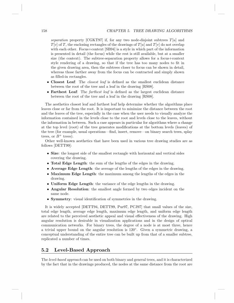
158 CHAPTER 5. TREE DRAWING ALGORITHMS
separation property [CGKT97] if, for any two node-disjoint subtrees T [u] andT [v] of T , the enclosing rectangles of the drawings of T [u] and T [v] do not overlapwith each other. Focus+context [SB94] is a style in which part of the informationis presented in detail (the focus) while the rest is still available, but at a smallersize (the context). The subtree-separation property allows for a focus+contextstyle rendering of a drawing, so that if the tree has too many nodes to fit inthe given drawing area, then the subtrees closer to focus can be shown in detail,whereas those farther away from the focus can be contracted and simply shownas filled-in rectangles.
• Closest Leaf: The closest leaf is defined as the smallest euclidean distancebetween the root of the tree and a leaf in the drawing [RS08].
• Farthest Leaf: The farthest leaf is defined as the largest euclidean distancebetween the root of the tree and a leaf in the drawing [RS08].
The aesthetics closest leaf and farthest leaf help determine whether the algorithms placeleaves close or far from the root. It is important to minimize the distance between the rootand the leaves of the tree, especially in the case when the user needs to visually analyze theinformation contained in the levels close to the root and levels close to the leaves, withoutthe information in between. Such a case appears in particular for algorithms where a changeat the top level (root) of the tree generates modifications at the bottom levels (leaves) ofthe tree (for example, usual operations—find, insert, remove—on binary search trees, splaytrees, or B+ trees).
Other well-known aesthetics that have been used in various tree drawing studies are asfollows [DETT99]:
• Size: the longest side of the smallest rectangle with horizontal and vertical sidescovering the drawing.
• Total Edge Length: the sum of the lengths of the edges in the drawing.
• Average Edge Length: the average of the lengths of the edges in the drawing.
• Maximum Edge Length: the maximum among the lengths of the edges in thedrawing.
• Uniform Edge Length: the variance of the edge lengths in the drawing.
• Angular Resolution: the smallest angle formed by two edges incident on thesame node.
• Symmetry: visual identification of symmetries in the drawing.
It is widely accepted [DETT94, DETT99, Pur97, PCJ97] that small values of the size,total edge length, average edge length, maximum edge length, and uniform edge lengthare related to the perceived aesthetic appeal and visual effectiveness of the drawing. Highangular resolution is desirable in visualization applications and in the design of opticalcommunication networks. For binary trees, the degree of a node is at most three, hencea trivial upper bound on the angular resolution is 120. Given a symmetric drawing, aconceptual understanding of the entire tree can be built up from that of a smaller subtree,replicated a number of times.
5.2 Level-Based Approach
The level-based approach can be used on both binary and general trees, and it is characterizedby the fact that in the drawings produced, the nodes at the same distance from the root are

5.2. LEVEL-BASED APPROACH 159
horizontally aligned. Algorithms based on this approach are usually simple to understandand implement and produce intuitive drawings that exhibit clear display of symmetries.However, these algorithms have two disadvantages: the drawing has an area of Ω(n2) and,for balanced trees with many nodes, the width is much larger than the height.
Level-based algorithms have been designed previously [Blo93, RT81, BJL02, Wal90]. Thealgorithms described in [BJL02, Wal90] achieve better area, but they do not exhibit thesubtree separation property.
A recursive algorithm for binary trees [RT81], which exhibits the subtree separationproperty, uses the following steps: draw the subtree rooted at the left child, draw thesubtree rooted at the right child, place the drawings of the subtrees at horizontal distance2, and place the root one level above and halfway between the children. If there is only onechild, place the root at horizontal distance 1 from the child. A drawing produced by thisalgorithm is provided in Figure 5.2.
Figure 5.2 Drawing of the Fibonacci tree with 88 nodes, generated by the level-basedalgorithm of [RT81].
By using a geometric transformation (cartesian → polar), level drawings yield radialdrawings , where nodes are placed on concentric circles by level (see Figure 5.3).
Figure 5.3 Example of a transformation from a level drawing to a radial drawing. Figuretaken from [CT].
Radial drawings are often used in drawing graphs, even though they do not always guar-antee planarity. Several algorithms for radial drawings of trees have been designed, andsome of them have also been used in various applications [Ber81, Ead92, CPM+98, CPP00,BM03, Bac07].

160 CHAPTER 5. TREE DRAWING ALGORITHMS
5.3 H-V Approach
The horizontal-vertical approach can be used on both binary and general trees. In thisapproach, a divide-and-conquer strategy is used to recursively construct an upward, or-thogonal, and straight-line drawing of a tree, by placing the root of the tree in the top-leftcorner, and the drawings of its left and right subtrees one next to the other (horizontalcomposition) or one below the other (vertical composition) (see Figure 5.4). The resultingdrawing also exhibits the subtree separation property within an O(n log n) area.
(a) (b)
Figure 5.4 General H-V approach. (a) Horizontal composition: the drawings of the sub-trees rooted at the children of o are placed one next to the other. (b) Vertical composition:the drawings of the subtrees rooted at the children of o are placed one below the other.
Various H-V algorithms can be obtained, depending on which layout is used and whatother conditions are imposed on the drawing. An algorithm using this approach has beendeveloped for binary trees [CDP92]. This algorithm places the drawing of the subtreewith the greater width one unit below the drawing of the subtree with the smaller width(see Figure 5.4(b)). A modification of this algorithm, in which vertical and horizontalcombinations are used alternatively, produces area-efficient drawings of complete, AVL,and Fibonacci trees. The algorithm can easily be extended to general trees.
5.4 Path-Based Approach
The path-based approach uses a recursive winding paradigm to draw a binary tree T by layingdown a small chain of nodes monotonically in the x-direction leading to a distinguished nodev, and then “winding” by recursively laying out the subtrees rooted at the children of v inthe opposite direction.
Several path-based algorithms have been designed [CGKT02, GR03a, SKC00].Recursively, for every subtree rooted at a node v, a parameter A is fixed, so that, if
n(v) ≤ A, then the drawings of the subtrees rooted at the children of v are placed one nextto the other, as in Figure 5.5 (a). Otherwise, the subtree looks like Figure 5.5 (b), wherev1 is the root of the subtree, vi+1 = r(vi) for i ≥ 1, k ≥ 1 is the first index for whichn(vk) > n − A and n(vk+1) ≤ n − A, Ti is the subtree rooted at l(vi), T
′ = l(vk), andT ′′ = r(vk). In the second case, depending on whether an upward or a non-upward drawingis to be obtained, the drawings are placed as in Figures 5.6(a) and 5.6(b), respectively.The user controls the aspect ratio by modifying parameter A.

5.4. PATH-BASED APPROACH 161
(a) (b)
Figure 5.5 (a) When n(v) ≤ A, the subtrees are placed one next to the other. (b) Whenn(v) > A, the tree is divided into subtrees T1, T2, . . . , Tk−2, Tk−1, T
′, T ′′.
(a) (b)
Figure 5.6 (a) Upward drawing of binary tree T . (b) Non-upward drawing of binarytree T .
A drawing of the Fibonacci tree with 88 nodes produced by the algorithm of Chan etal. [CGKT02], with the value for the parameter A at one of the extremes, is provided inFigure 5.7. This algorithm produces the best worst-case theoretical bound on area forpath-based algorithms: O(n log log n).
Figure 5.7 Drawing of Fibonacci tree with 88 nodes produced by the path-based algo-rithm [CGKT02], with parameter A at one of the extremes: A = 88.

162 CHAPTER 5. TREE DRAWING ALGORITHMS
5.5 Ringed Circular Layout Approach
In these algorithms, children are placed on the circumference or the interior of a circle cen-tered at their parents [GADM04, CC99, Ead92, MH98, MMC99, TM02, RSJ07]. In general,these algorithms are used to draw high-degree trees. However, the resulting drawings areoften not planar. An example of the general idea of the approach is provided in Figure 5.8.
Figure 5.8 General idea for the ringed circular layout approach.
Cone trees [RMC91] are a 3D extension of the 2D ringed circular layout approach. Incone trees, the parent is located at the tip of a cone, and its children are spaced equally onthe bottom circle of the cone.
5.6 Separation-Based Approach
The separation-based approach can be used on both binary and general trees. Separation-based algorithms have been designed [GR02, GR03b, GR03c, RS07]. In this approach, adivide-and-conquer strategy is used to recursively construct a drawing of a tree, by per-forming the following actions at each recursive step:
• Find a Separator Edge or a Separator Node: A separator edge (node) of a tree Twith degree(T ) = d is an edge (node), which, if removed, divides T into at mostd smaller, partial, trees. It has been shown that every tree contains a separatoredge or a separator node [GR03c, Val81].
• Split Tree: Split T into at most d partial trees by removing a separator edge ora separator node.
• Assign Aspect Ratios: Preassign a desirable aspect ratio to each partial tree.
• Draw Partial Trees: Recursively construct a drawing of each partial tree usingits preassigned aspect ratio.
• Compose Drawings: Arrange the drawings of the partial trees, and draw thenodes and edges that were removed from the tree to divide it, such that thedrawing of the tree thus obtained meets certain aesthetics.

5.7. ALGORITHMS FOR DRAWING BINARY TREES 163
5.7 Algorithms for Drawing Binary Trees
A binary tree is one where each node has at most two children. Most of the research ondrawing trees targets binary trees; hence, in this section, several algorithms for drawingbinary trees are presented.
Binary trees have a strong connection to real-life applications. For instance, binarytrees represent programs in combinatory logic, which is under investigation as an approachto nanostructure synthesis and control [Mac03]. The idea is to use molecular processesto implement the combinatory logic tree substitution operations, so that the molecularreorganization of the trees results in the desired structure or process. Visualization ofthese binary trees could improve the investigator’s ability in interpreting the substitutionoperations involved in combinatory logic.
5.7.1 Theoretical Results
We summarize some known theoretical results on planar grid drawings of binary trees. (SeeTable 5.1.)
Drawing Type Area Aspect Ratio Reference
upward orthogonalpolyline O(n log log n) Θ(log2 n/(n log log n)) [GGT96]
(non-upward) orthogonalpolyline O(n) Θ(1) [Lei80, Val81]
upward orthogonalstraight-line O(n log n) [1, n/ log n] [CDP92, CGKT02]
(non-upward) orthogonalstraight-line O(n log log n) Θ(log2 n/(n log log n)) [CGKT02, SKC00]
upward polyline O(n) [n−ǫ, nǫ] [GGT96]upward straight-line O(n log log n) Θ(log2 n/(n log log n)) [SKC00]
(non-upward) straight-line O(n) [n−ǫ, nǫ] [GR04]
Table 5.1 Bounds on the areas and aspect ratios of various kinds of planar grid drawingsof an n-node unordered binary tree. Here, ǫ is an arbitrary constant, such that 0 < ǫ < 1.
Let T be an n-node binary tree. Garg et al. [GGT96] present an algorithm for constructingan upward polyline drawing of T with O(n) area, and any user-specified aspect ratio in therange [n−ǫ, nǫ], where ǫ is any constant, such that 0 < ǫ < 1. It also shows that n log log nis a tight bound for the area of upward orthogonal polyline drawings, i.e., any binary treecan be drawn in this fashion in O(n log log n) area, and there exists a family of binary treesthat requires Ω(n log log n) area in any such drawing. Leiserson [Lei80] and Valiant [Val81]present algorithms for constructing a (non-upward) orthogonal polyline drawing of T withO(n) area. Chan et al. [CGKT02] give an algorithm for constructing an upward orthogonalstraight-line drawing of T with O(n log n) area, and any user-specified aspect ratio in therange [1, n/ log n]. It also shows that n log n is a tight bound for such drawings. Shin etal. [SKC00] give an algorithm for constructing an upward straight-line drawing of T withO(n log log n) area. Chan et al. [CGKT02] and Shin et al. [SKC00] show that T admitsa non-upward planar straight-line orthogonal grid drawing with height O(n/A) logA andwidth O(A+ log n), where 2 ≤ A ≤ n is any user-specified number. This result also implies

164 CHAPTER 5. TREE DRAWING ALGORITHMS
that we can draw any binary tree in this fashion in area O(n log log n) (by setting A = log n).If T is a Fibonacci tree (AVL tree and complete binary tree), then Crescenzi et al. [CDP92]and Trevisan [Tre96] (Crescenzi et al. [CPP98, CDP92], respectively) give algorithms forconstructing an upward straight-line drawing of T with O(n) area. Garg and Rusu [GR04]present an algorithm for constructing a (non-upward) straight-line drawing of T with O(n)area, and any user-specified aspect ratio in the range [n−ǫ, nǫ], where ǫ is any constant, suchthat 0 < ǫ < 1. This is trivially a tight bound, as any straight-line drawing of a binary treewith n nodes requires Ω(n) area.
Table 5.2 summarizes the results for order-preserving algorithms.
Drawing Type Area Aspect Ratio Ref.
Complete tree
upward straight-line order-preserving
Θ(n) O(1) [CDP92]
Fibonacci tree
upward straight-line order-preserving
Θ(n) O(1) [Tre96]
Special balanced binary tree such as red-black
upward straight-line order-preserving
O(n(log log n)2) n/ log2 n [SKC00]
Logarithmic tree
upward straight-line order-preserving
Θ(n) O(1) [CP98]
Binary tree
upward orthogonalpolyline order-preserving
O(n log n) Θ(log2 n/(n log log n)) [Kim95, GGT96]
non-upward orthogonalpolyline order-preserving
O(n) (9a+ 8)/(9b+ 8) [DT81]
upward orthogonalstraight-lineorder-preserving
Θ(n2) O(1) [CDP92, Fra07]
non-upward orthogonalstraight-lineorder-preserving
O(n1.5) O(√
(n)/n) [Fra07]
upward polylineorder-preserving
O(n log n) log n/n [Kim04]
O(n log n) Θ(log2 n/(n log log n)) [GGT96, CDP92]non-upward polylineorder-preserving
O(n log log n) (n log log n)/ log2 n [GR03a]
upward straight-lineorder-preserving
Θ(n log n) n/ log n [GR03a]
non-upward straight-lineorder-preserving
O(n log n) [1, n/ log n] [GR03a]
O(n log log n) (n log log n)/ log2 n [GR03a]
Table 5.2 Bounds on the areas and aspect ratios of various kinds of order-preservingplanar grid drawings of an n-node ordered tree. Here, ab ≤ kn, where k is some constant.
Shin et al. [SKC00] have shown that a special class of balanced binary trees, which in-cludes k-balanced, red-black, BB[α], and (a, b) trees, admits order-preserving planar upward
5.7. ALGORITHMS FOR DRAWING BINARY TREES 165
straight-line grid drawings with area O(n(log log n)2). Crescenzi et al. [CDP92], Crescenziand Penna [CP98], and Trevisan [Tre96] give order-preserving planar upward straight-linegrid drawings of complete, logarithmic, and Fibonacci trees, respectively, with area O(n).Dolev and Trickey [DT81] prove that binary trees admit Θ(n) area order-preserving or-thogonal drawings. Kim [Kim95] shows an upper bound of O(n log n) area for upwardorder-preserving orthogonal drawings of ternary trees (trees whose nodes have at mostthree children), result that immediately extends to binary trees. This area bound is opti-mal, as Garg et al. [GGT96] demonstrate a lower bound of O(n log n) area for such drawingsof binary trees. Crescenzi et al. [CDP92] give an algorithm that achieves O(n2) area forupward orthogonal straight-line order-preserving drawings of binary trees. Frati [Fra07]proves that this bound is optimal. Frati [Fra07] also gives the best known upper bound ofO(n1.5) area for non-upward orthogonal straight-line order-preserving drawings of binarytrees. It is unknown whether this is an optimal bound, as the trivial O(n) is the lower boundcurrently known. Garg et al. [GGT96] provides an algorithm that constructs an upwardpolyline order-preserving drawing of a binary tree with O(n log n) area, which is the opti-mal bound for such drawings [CDP92]. Kim [Kim04] improves the number of bends fromO(n) to O(n/ log n), while matching the area bound. Garg and Rusu [GR03a] show that abinary tree admits an order-preserving planar straight-line grid drawing with O(n log log n)area. In addition, they show that a binary tree admits an order-preserving upward planarstraight-line drawing with optimal O(n log n) area.
A variety of results exist for other kinds of drawings. Di Battista et al. [DETT99] andFrati [Fra09] have given a survey of these results.
5.7.2 Experimental Analysis
Experimental studies provide insight into the behavior of tree drawing algorithms beyondtheir targetted aesthetic criteria. In a comprehensive experimental study [RS08], separation-based algorithm by Garg and Rusu [GR04], path-based algorithm by Chan et al. [CGKT02],level-based algorithm by Reingold and Tilford [RT81], and ringed circular layout algorithmby Teoh and Ma [TM02] were compared on a large suite of seven types of binary treesof various sizes, based on ten quality measures: area, aspect ratio, size, total edge length,average edge length, maximum edge length, uniform edge length, angular resolution, closestleaf, and farthest leaf. As the specific algorithms compared are intended to be representa-tive of their respective approaches, it is expected that the results generally apply to otheralgorithms using the same approach and even extend to trivial extensions to general trees.
This experimental analysis includes some interesting findings:
• The performance of a drawing algorithm on a tree-type is not a good predic-tor of the performance of the same algorithm on other tree-types: some of thealgorithms perform best on a tree-type, and worst on other tree-types.
• Reingold-Tilford algorithm [RT81] scores worse in comparison to the other chosenalgorithms for almost all ten aesthetics considered.
• The intuition that low average edge length and area go together is contradictedin only one case.
• The intuitions that average edge length and maximum edge length, uniform edgelength and total edge length, and short maximum edge length and close farthestleaf go together are contradicted for unbalanced binary trees.
• With regards to area, of the four algorithms studied, three perform best ondifferent types of trees.

166 CHAPTER 5. TREE DRAWING ALGORITHMS
• With regards to aspect ratio, of the four algorithms studied, three perform wellon trees of different types and sizes.
• Not all algorithms studied perform best on complete binary trees even thoughthey have one of the simplest tree structures.
• The level-based algorithm of Reingold-Tilford [RT81] produces much worse as-pect ratios than algorithms designed using other approaches.
• The path-based algorithm of Chan et al. [CGKT02] tends to construct drawingswith better area at the expense of worse aspect ratio.
5.7.3 Unordered Trees
In this section, we present the algorithm of [GR04] in more detail. This algorithm uses aseparation-based approach (therefore, we call it Separation), and achieves optimal lineararea for planar straight-line grid drawings, while at the same time, giving the user controlover the aspect ratio. In addition, the drawings produced by this algorithm exhibit thesubtree separation property.
Let T be a tree with root o. Let n be the number of nodes in T . A partial tree of T is aconnected subgraph of T .
For some trees, the algorithm designates a special link node u∗ that has at most one child.
Let T be a tree with link node u∗. A planar straight-line grid drawing Γ of T is a feasibledrawing of T , if it has the following three properties:
• Property 1: The root o is placed at the top-left corner of Γ.
• Property 2: If u∗ 6= o, then u∗ is placed at the bottom boundary of Γ. Moreover,u∗ can move downward in its vertical channel by any distance without causingany edge-crossings in Γ.
• Property 3: If u∗ = o, then no other node or edge of T is placed on or crosses thevertical and horizontal channels occupied by o. Moreover, u∗ (i.e., o) can moveupward in its vertical channel by any distance without causing any edge-crossingsin Γ.
Let A and ǫ be two numbers, where ǫ is a constant, such that 0 < ǫ < 1, and n−ǫ ≤ A ≤ nǫ.A is called the desirable aspect ratio for T .
Theorem 5.1 [Separator Theorem [Val81]] Every binary tree T with n nodes, where n ≥ 2,contains an edge e, called a separator edge, such that removing e from T splits it into twonon-empty trees with n1 and n2 nodes, respectively, such that for some x, where 1/3 ≤ x ≤2/3, n1 = xn, and n2 = (1− x)n. Moreover, e can be found in O(n) time.
The algorithm takes ǫ, A, and T as input and uses a divide-and-conquer strategy torecursively construct a feasible drawing Γ of T , by performing the following actions at eachrecursive step:
• Split Tree: Split T into at most five partial trees by removing at most two nodesand their incident edges from it. Each partial tree has at most (2/3)n nodes.Based on whether the separator edge is on the leftmost path of T or not, thereare two general cases, which are shown in Figure 5.9.
• Assign Aspect Ratios: Correspondingly, assign a desirable aspect ratio Ak to eachpartial tree Tk. The value of Ak is based on the value of A and the number ofnodes in Tk.

5.7. ALGORITHMS FOR DRAWING BINARY TREES 167
• Draw Partial Trees: Recursively construct a feasible drawing of each partial treeTk with Ak as its desirable aspect ratio.
• Compose Drawings: Arrange the drawings of the partial trees, and draw thenodes and edges that were removed from T to split it, such that the drawing Γof T is a feasible drawing. Note that the arrangement of these drawings is donebased on the cases shown in Figure 5.9. In each case, if A < 1, then the drawingsof the partial trees are stacked one above the other, and if A ≥ 1, then they areplaced side-by-side.
Remark: The drawing Γ constructed by the algorithm may not have aspect ratio exactlyequal to A, but it fits inside a rectangle with area O(n) and aspect ratio A.
(a)
(b)
Figure 5.9 (a) Drawing T in Case 1 (when the separator (u, v) is not in the leftmostpath of T ). (b) Drawing T in Case 2 (when the separator (u, v) is in the leftmost path ofT ). For each case, first the structure of T for that case is shown, then its drawing whenA < 1, and then its drawing when A ≥ 1. For simplicity, p(a) and p(u) are shown to be inthe interior of ΓA, but actually, either they are the same as o, or if A < 1 (A ≥ 1), thenthey are placed at the bottom (right) boundary of ΓA. For simplicity, ΓA, ΓB , and ΓC areshown as identically sized boxes, but in actuality, they may have different sizes.
Figure 5.10 (a) shows a drawing of a complete binary tree with 63 nodes constructed byalgorithm Separation, with A = 1 and ǫ = 0.5. Figure 5.10 (b) shows a drawing of a treewith 63 nodes, consisting of a single path, constructed by algorithm Separation, with A = 1and ǫ = 0.5.
Split Tree
The splitting of tree T into partial trees is done as follows:

168 CHAPTER 5. TREE DRAWING ALGORITHMS
(a) (b)
Figure 5.10 (a) Drawing of the complete binary tree with 63 nodes constructed by Algo-rithm Separation, with A = 1 and ǫ = 0.5. (b) Drawing of a tree with 63 nodes, consistingof a single path, constructed by Algorithm Separation, with A = 1 and ǫ = 0.5.
• Order the children of each node such that u∗ becomes the leftmost node of T .
• Using Theorem 5.1, find a separator edge (u, v) of T , where u is the parent of v.
• Based on whether (u, v) is in the leftmost path of T , there are two general cases(each with several subcases—not covered here):
– Case 1: The separator edge (u, v) is not in the leftmost path of T . Let obe the root of T . Let a be the last node common to the path o v, andthe leftmost path of T . Let partial trees TA, TB , TC , Tα, Tβ , T1, and T2 bedefined as follows (see Figure 5.9 (a)):
∗ If o 6= a, then TA is the maximal partial tree with root o, that containsp(a), but does not contain a. If o = a, then TA = ∅.
∗ TB is the subtree rooted at r(a).
∗ If u∗ 6= a, then TC is the subtree rooted at l(a). If u∗ = a, then TC = ∅.∗ If s(v) exists, i.e., if v has a sibling, then T1 is the subtree rooted ats(v). If v does not have a sibling, then T1 = ∅.
∗ T2 is the subtree rooted at v.
∗ If u 6= a, then Tα is the subtree rooted at u. If u = a, then Tα = T2.Note that Tα is a subtree of TB .
∗ If u 6= a and u 6= r(a), then Tβ is the maximal partial tree with rootr(a), that contains p(u), but does not contain u. If u = a or u = r(a),then Tβ = ∅. Again, note that Tβ belongs to TB .
Nodes a and u and their incident edges are being removed to split T intoat most five partial trees TA, TC , Tβ , T1, and T2. p(a) is designated as thelink node of TA, p(u) as the link node of Tβ , and u∗ as the link node of TC .Arbitrarily select a leaf of T1, and a leaf of T2, and designate them as thelink nodes of T1 and T2, respectively.
– Case 2: The separator edge (u, v) is in the leftmost path of T . Let o bethe root of T . Let partial trees TA, TB , and TC be defined as follows (seeFigure 5.9 (b)):
∗ If o 6= u, then TA is the maximal partial tree with root o, that containsp(u), but does not contain u. If o = u, then TA = ∅.

5.7. ALGORITHMS FOR DRAWING BINARY TREES 169
∗ If r(u) exits, i.e., u has a right child, then TB is the subtree rooted atr(u). If u does not have a right child, then TB = ∅.
∗ TC is the subtree rooted at v.
Node u and its incident edges are being removed to split T into at mostthree partial trees TA, TB , and TC . p(u) is designated as the link nodeof TA, and u∗ as the link node of TC . Arbitrarily select a leaf of TB anddesignate it as the link node of TB .
Assign Aspect Ratios
Let Tk be a partial tree of T , where for Case 1, Tk is either TA, TC , Tβ , T1, or T2, andfor Case 2, Tk is either TA, TB , or TC . Let nk be the number of nodes in Tk.
Definition: Tk is a large partial tree of T if:
• A ≥ 1 and nk ≥ (n/A)1/(1+ǫ), or
• A < 1 and nk ≥ (An)1/(1+ǫ),
and is a small partial tree of T otherwise.In Step Assign Aspect Ratios, a desirable aspect ratio Ak is assigned to each non-empty
Tk as follows: Let xk = nk/n.
• If A ≥ 1: If Tk is a large partial tree of T , then Ak = xkA, otherwise (i.e., if Tk
is a small partial tree of T ) Ak = n−ǫk .
• If A < 1: If Tk is a large partial tree of T , then Ak = A/xk, otherwise (i.e., if Tk
is a small partial tree of T ) Ak = nǫk.
Intuitively, the above assignment strategy ensures that each partial tree gets a gooddesirable aspect ratio.
Draw Partial Trees
If A ≥ 1, then the values of AA and Aβ (AA and Aβ are the desirable aspect ratiosfor TA and Tβ , respectively) are being changed to 1/AA and 1/Aβ , respectively. This isdone so because later in Step Compose Drawings, when constructing Γ, if A ≥ 1, then thedrawings of TA and Tβ are rotated by 90. Drawing TA and Tβ with desirable aspect ratios1/AA and 1/Aβ , respectively, compensates for the rotation, and ensures that the drawingsof TA and Tβ that eventually get placed within Γ are those with desirable aspect ratios AA
and Aβ , respectively.Next, each non-empty partial tree Tk, k ∈ A,B,C, α, β, 1, 2, is drawn recursively with
Ak as its desirable aspect ratio. The base case for the recursion happens when Tk containsexactly one node, in which case, the drawing of Tk is simply the one consisting of exactlyone node.
Compose Drawings
Let Γk denote the drawing of a partial tree Tk constructed in Step Draw PartialTrees. We now describe the construction of a feasible drawing Γ of T from the drawings ofits partial trees in Case 1.
In Case 1, first a drawing Γα of the partial tree Tα is constructed by composing Γ1 andΓ2 as shown in Figure 5.11, then a drawing ΓB of TB is constructed by composing Γα andΓβ as shown in Figure 5.12, and finally Γ is constructed by composing ΓA, ΓB , and ΓC asshown in Figure 5.9 (a).
In the general case (u 6= a and T1 6= ∅), Γα is constructed as follows (see Figure 5.11):

170 CHAPTER 5. TREE DRAWING ALGORITHMS
Figure 5.11 Drawing Tα in the general case (u 6= a and T1 6= ∅). First, the structureof Tα is shown, then its drawing when A < 1, and then its drawing when A ≥ 1. Forsimplicity, Γ1 and Γ2 are shown as identically sized boxes, but in actuality, their sizes maybe different.
• If A < 1, then Γ1 is placed above Γ2 such that the left boundary of Γ1 is one unitto the right of the left boundary of Γ2; u is placed in the same vertical channelas v and in the same horizontal channel as s(v).
• If A ≥ 1, then Γ1 is placed one unit to the left of Γ2, such that the top boundaryof Γ1 is one unit below the top boundary of Γ2; u is placed in the same verticalchannel as s(v) and in the same horizontal channel as v.
Draw edges (u, s(v)) and (u, v).
Figure 5.12 Drawing TB in the general case (Tβ 6= ∅). First, the structure of TB isshown, then its drawing when A < 1, and then its drawing when A ≥ 1. For simplicity,p(u) is shown to be in the interior of Γβ , but actually, it is either same as r(a), or if A < 1(A ≥ 1), then is placed on the bottom (right) boundary of Γβ . For simplicity, Γβ and Γα
are shown as identically sized boxes, but in actuality, their sizes may be different.
In the general case (Tβ 6= ∅), ΓB is constructed as follows (see Figure 5.12):
• if A < 1, then Γβ is placed one unit above Γα such that the left boundaries ofΓβ and Γα are aligned.
• If A ≥ 1, then first Γβ is rotated clockwise by 90 and then flipped right-to-left,then Γβ is placed one unit to the left of Γα such that the top boundaries of Γβ
and Γα are aligned.
Draw edge (p(u), u).In general Case 1, Γ is constructed from ΓA, ΓB , and ΓC as follows (see Figure 5.9 (a)):
• If A < 1, then ΓA, ΓB , and ΓC are stacked one above the other, such that theyare separated by unit distance from each other, and the left boundaries of ΓA
and ΓC are aligned with each other and are placed one unit to the left of the leftboundary of ΓB ; a is placed in the same vertical channel as o and l(a), and inthe same horizontal channel as r(a).
• If A ≥ 1, then first ΓA is rotated clockwise by 90 and flipped right-to-left.Then, ΓA, ΓC , and ΓB are placed from left-to-right in that order, separated by

5.7. ALGORITHMS FOR DRAWING BINARY TREES 171
unit distances, such that the top boundaries of ΓA and ΓB are aligned with eachother, and are one unit above the top boundary of ΓC . Then, ΓC is moved downuntil u∗ becomes the lowest node of Γ; a is placed in the same vertical channelas l(a) and in the same horizontal channel as o and r(a).
Draw edges (p(a), a), (a, r(a)), and (a, l(a)).
In general Case 2, Γ is constructed by composing ΓA, ΓB , and ΓC , using a procedure similarto the one of Case 1 (see Figure 5.9(b)).
Theorem 5.2 Let T be a binary tree with n nodes. Given two numbers A and ǫ, whereǫ is a constant, such that 0 < ǫ < 1, and n−ǫ ≤ A ≤ nǫ, a planar straight-line grid drawingof T with O(n) area and aspect ratio A, can be constructed in O(n log n) time. Moreover,Γ has the subtree-separation property.
Proof: Designate any leaf of T as its link node. Construct a drawing Γ of T by invokingAlgorithm Separation with T , A, and ǫ as input. Γ will be a planar straight-line grid drawingcontained entirely within a rectangle with O(n) area and aspect ratio A, and which exhibitsthe subtree separation property.
5.7.4 Ordered Trees
In this Section, we present two algorithms of [GR03a] in detail. The first algorithm (wecall it Fixed Spine) shows that a binary tree admits an order-preserving upward planarstraight-line grid drawing with optimal O(n log n) area. The second algorithm (we call itArbitrary Spine), shows that a binary tree admits an order-preserving planar straight-linegrid drawing with width O(A+ log n), height O((n/A) logA), and area O(n log n), for anygiven 2 ≤ A ≤ n. Setting A = log n, it results in an area of O(n log log n). Both algorithmstake O(n) time to construct the drawings.
Let T be an ordered tree. Each node of T has at most two children, called its left andright children, respectively.
Let α be a positive integer. An order-preserving planar straight-line grid drawing of T isan α-drawing of T , if it has the following two properties:
• Property 1: No node is placed to the left of, or above the root of, T .
• Property 2: The vertical and horizontal separations between the root and itsrightmost child are equal to α and one units, respectively.
A left-corner drawing of an ordered tree is an order-preserving planar straight-line griddrawing, where no node of the tree is placed to the left of, or above its root. Note that anα-drawing is also a left-corner drawing.
The mirror-image of T is the ordered tree obtained by reversing the counterclockwiseorder of edges incident on each node.
A spine of T is a path v0v1v2 . . . vm, where v0, v1, v2, . . . , vm are nodes of T , that is definedrecursively as follows (see Figure 5.13):
• v0 is the same as the root of T ;
• vi+1 is a child of vi, such that the subtree rooted at vi+1 has the maximumnumber of nodes among all the subtrees that are rooted at the children of vi.
A non-spine node of T is one that does not belong to its spine.

172 CHAPTER 5. TREE DRAWING ALGORITHMS
(a) (b)
Figure 5.13 (a) A binary tree T with spine v0v1 . . . v13. (b) The order-preserving planarupward straight-line grid drawing of T constructed by fixed spine algorithm.
Algorithm Fixed Spine
For simplicity, throughout this section, it is assumed that each non-leaf node hasexactly two children. The algorithm can be simply extended to cover the case where anon-leaf node has only one child.
The fixed spine drawing algorithm uses a path-based approach to obtain an order-preservingupward planar straight-line grid drawing with optimal (O(n log n)) area of an ordered bi-nary tree T . In each recursive step, it breaks T into several subtrees, draws each subtreerecursively, and then combines their drawings to obtain an upward α-drawing D(T ) of T ,where α is a positive integer given as a parameter to the algorithm.
Let P = v0v1v2 . . . vm be a spine of T .There are two cases (see Figures 5.14 and 5.15):
• Case 1: v1 is the left child of v0 (see Figure 5.14(a)).Let L be the subtree rooted at v1, s be the non-spine child of v0, and R be the

5.7. ALGORITHMS FOR DRAWING BINARY TREES 173
subtree rooted at s. v0 is placed at the origin. 1-drawings D(L) and D(R) ofL and R are recursively constructed. D(R) is placed such that s is one unit tothe right of, and α units below v0. D(L) is placed such that v1 is in the samevertical channel as v0, and is one unit below D(R) (see Figure 5.14(b)).
(a) (b)
Figure 5.14 (a) The structure of a binary tree T in Case 1, where v1 is the left child ofv0. (b) The drawing of T in Case 1. For simplicity, D(L) and D(R) are shown as identicallysized boxes, but in actuality, they may have different sizes.
• Case 2: v1 is the right child of v0 (see Figure 5.15(a)).Let k ≥ 1 be the smallest integer, such that vk is either a leaf, or has a non-spinenode as its left child.There are two subcases:
– vk has a non-spine node as its left child: Let s0, s1, . . . , sk be the non-spinechildren of v0, v1, . . . , vk, respectively. Let L, A, and B be the subtreesrooted at s0, sk, and vk+1, respectively. Let R1, R2, . . . , Rk−1 be the sub-trees rooted at s1, s2, . . . , sk−1, respectively. T is drawn as shown in Fig-ure 5.15(b). v0 is placed at the origin. v1 is placed one unit to the right of,and α units below, v0. 1-drawings D(L), D(A), D(R1), D(R2), . . . , D(Rk−1)of L,A,R1, R2, . . . , Rk−1, respectively, are recursively constructed. D(R1)is placed one unit to the right of, and one unit below, v1. For each i, where2 ≤ i ≤ k−1, vi and D(Ri) are placed such that vi is in the same horizontalchannel as the bottom of D(Ri−1) and is in the same vertical channel asvi−1, and D(Ri) is one unit to the right of, and one unit below, vi. Nodevk is placed in the same vertical channel as vk−1, and in the same hori-zontal channel as the bottom of D(Rk−1). D(A) is placed one unit belowvk, such that sk is in the same vertical channel as vk. D(L) is placed oneunit below D(A), such that s0 is in the same vertical channel as v0. Letβ = h(D(A))+h(D(L))+2, where h(D(A)) and h(D(L)) denote the heightsof D(A) and D(L), respectively. Let G be the drawing with the maximumwidth amongD(L), D(A), D(R1), D(R2), . . . , D(Rk−1). LetW be the widthof G. A β-drawing of the mirror image of B is recursively constructed, andthen flipped right-to-left to obtain a drawing D(B) of B. D(B) is placedsuch that vk+1 is one unit below vk, and maxW +3, width of D(B) unitsto the right of v0.
– vk is a leaf: T is drawn in a similar fashion as in the previous subcase,except that D(A) and D(B) do not exist.

174 CHAPTER 5. TREE DRAWING ALGORITHMS
(a) (b)
Figure 5.15 The structure of a binary tree T in Case 2, where v1 is the right child ofv0: (a) vk has a non-spine node as its left child; (b) the drawing of T , when vk has anon-spine node as its left child. For simplicity, D(A), D(L), D(R1), . . . , D(Rk−1) are shownas identically sized boxes, but in actuality, they may have different sizes.
Theorem 5.3 An ordered binary tree with n nodes admits an order-preserving up-ward planar straight-line grid drawing with height at most n, width O(log n), and optimalO(n log n) area, which can be constructed in O(n) time.
Proof: Let T be an n-node ordered binary tree. Using the above algorithm, construct a1-drawing D(T ) of T in O(n) time. As discussed above, D(T ) will be an order-preservingupward planar straight-line grid drawing of T with height at most n, width O(log n), andoptimal O(n log n) area.
LEMMA 5.1 A left-corner drawing of an n-node ordered binary tree with area O(n log n),height O(log n), and width at most n, can be constructed in O(n) time.
Proof: First a 1-drawing of the mirror image of T is constructed using Theorem 5.3,then it is rotated clockwise by 90, and then it is flipped right-to-left.
Algorithm Arbitrary Spine
For any user-defined number A, where 2 ≤ A ≤ n, algorithm Arbitrary Spine uses apath-based approach to construct an order-preserving planar straight-line grid drawing ofT with O((n/A) logA) height and O(A + log n) width. Thus, by setting the value of A,users can control the aspect ratio of the drawing. This implies that, by setting A = log n,such a drawing can be constructed with area O(n log log n).
An order-preserving planar straight-line grid drawing of a binary tree T is called a feasibledrawing, if the root of T is placed on the left boundary and no node of T is placed betweenthe root and the upper-left corner of the enclosing rectangle of the drawing. Note that aleft-corner drawing is also a feasible drawing.

5.7. ALGORITHMS FOR DRAWING BINARY TREES 175
Let n be the number of nodes in T . Let 2 ≤ A ≤ n be any number given as a parameterto the algorithm.
Figure 5.16 shows the drawing of the tree of Figure 5.13(a) constructed by algorithmArbitrary Spine with A =
√n, using Lemma 5.1.
Figure 5.16 Drawing of the tree with n = 57 nodes of Figure 5.13(a) constructed by theAlgorithm Arbitrary Spine with A =
√n =
√57 = 7.55, using Lemma 5.1.
In each recursive step, the algorithm constructs a feasible drawing of a subtree T ′ of T . IfT ′ has at most A nodes in it, then it constructs a left-corner drawing of T ′ using Lemma 5.1such that the drawing has width at most m and height O(logm), where m is the number ofnodes in T ′. Otherwise, i.e., if T ′ has more than A nodes in it, then it constructs a feasibledrawing of T ′ as follows:
1. Let P = v0v1v2 . . . vq be a spine of T ′.
2. Let mi denote the number of nodes in the subtree of T ′ rooted at vi, where0 ≤ i ≤ q. Let vk be the node of P with the value for k such that mk > m − Aand mk+1 ≤ m − A (since T ′ has more than A nodes in it, and m0,m1, . . . ,mq
is a strictly decreasing sequence of numbers, such a k exists).
3. See Figures 5.17 and 5.18. Let Ti denote the subtree rooted at the non-spinechild of vi, where 0 ≤ i ≤ k− 1. Assume, for simplicity, that vk and vk+1 are notleaves (the algorithm can be easily extended to handle the case, where vk or vk+1
is a leaf). Let T ∗ and T+ denote the subtrees rooted at the non-spine childrenof vk and vk+1, respectively. Let T
′′ denote the subtree rooted at vk+1. Let T′′′
denote the subtree rooted at vk+2.
4. Place v0 at the origin.
5. There are two cases:
• k = 0: Recursively construct a feasible drawing D∗ of T ∗. Recursivelyconstruct a feasible drawing D+ of the mirror image of T+. Recursivelyconstruct a feasible drawing D′′′ of the mirror image of T ′′′. Let s0 be theroot of T ∗ and s1 be the root of T+.
T ′ is drawn as shown in Figure 5.17. If s0 is the left child of v0, then D∗
is placed one unit below v0, with its left boundary aligned with v0 (see

176 CHAPTER 5. TREE DRAWING ALGORITHMS
(a) (b)
(c) (d)
Figure 5.17 Case k = 0: (a) s0 is the left child of v0, and s1 is the left child of v1; (b) s0is the right child of v0, and s1 is the left child of v1; (c) s0 is the left child of v0, and s1 isthe right child of v1; (d) s0 is the right child of v0, and s1 is the right child of v1.
Figure 5.17(a,c)). If s0 is the right child of v0, then D∗ is placed one unitabove, and one unit to the right of v0 (see Figure 5.17(b,d)). Let W ∗,W+, and W ′′′ be the widths of D∗, D+, and D′′′, respectively. Place v1 inthe same horizontal channel as v0 to its right at the distance maxW ∗ +2,W++2,W ′′′ from it. Let B0 and C0 be the lowest and highest horizontalchannels, respectively, occupied by the subdrawing consisting of v0 and D∗.If s1 is the left child of v1, then D+ is flipped right-to-left, and placed oneunit below B0, and one unit to the left of v1 (see Figure 5.17(a,b)). If s1 isthe right child of v1, then D+ is flipped right-to-left, and placed one unitabove C0, and one unit to the left of v1 (see Figure 5.17(c,d)). Let B1 bethe lowest horizontal channel occupied by the subdrawing consisting of v0,D∗, v1 and D+. Flip D′′′ right-to-left, and place it one unit below B1, suchthat its right boundary is aligned with v1 (see Figure 5.17).
• k > 0: For each Ti, where 0 ≤ i ≤ k− 1, construct a left-corner drawing Di
of Ti using Lemma 5.1.
Recursively construct feasible drawings D∗ and D′′ of the mirror images ofT ∗ and T ′′, respectively.
T ′ is drawn as shown in Figure 5.18. If T0 is rooted at the left child of v0,then D0 is placed one unit below v0, with its left boundary aligned with v0.If T0 is rooted at the right child of v0, then D0 is placed one unit above,and one unit to the right of v0. Place each Di and vi, where 1 ≤ i ≤ k − 1,such that:
– vi is in the same horizontal channel as vi−1 and is one unit to the rightof Di−1, and
– if Ti is rooted at the left child of vi, then Di is placed one unit belowvi, with its left boundary aligned with vi, otherwise (i.e., if Ti is rootedat the right child of vi) Di is placed one unit above, and one unit to theright of vi.

5.7. ALGORITHMS FOR DRAWING BINARY TREES 177
(a) (b)
(c) (d)
Figure 5.18 Case k > 0: Here k = 4, s0, s1, and s3 are the left children of v0, v1, andv3, respectively, s2 is the right child of v2, T0, T1, T2, T3, and T ′′ are the subtrees rootedat v0, v1, v2, v3, and v5, respectively, s4 is the non-spine child of v4, and T ∗ is the subtreerooted at s4; (a) s4 is the left child of v4; (c) s4 is the right child of v4. For simplicity, boxesD0, D1, D2, D3 are drawn with same size, but in actuality, they may have different sizes.
Let Bk−1 and Ck−1 be the lowest and highest horizontal channels, respec-tively, occupied by the subdrawing consisting of v0, v1, v2, . . . , vk−1 andD0, D1, D2, . . . , Dk−1. Let d be the width of the subdrawing consistingof v0, v1, v2, . . . , vk−1 and D0, D1, D2, . . . , Dk−1. Let W ∗ and W ′′ be thewidths of D∗ and D′′, respectively.
Place vk to the right of and in the same horizontal channel as vk−1, such thatthe horizontal distance between vk and v0 is equal to maxd+1,W ∗+2,W ′′.If T ∗ is rooted at the left-child of vk, then D∗ is flipped right-to-left, andplaced one unit below Bk−1, and one unit left of vk (see Figure 5.18(b)).If T ∗ is rooted at the right-child of vk, then D∗ is flipped right-to-left,and placed one unit above Ck−1, and one unit to the left of vk (see Fig-ure 5.18(d)). Let Bk be the lowest horizontal channel occupied by the sub-drawing consisting of v1, v2, . . . , vk, and D0, D1, D2, . . . , Dk−1, D
∗. Flip D′′
right-to-left, and place it one unit below Bk, such that its right boundaryis aligned with vk (see Figure 5.18(b,d)).
Theorem 5.4 Let T be an ordered binary tree with n nodes. Let 2 ≤ A ≤ n be anynumber. T admits an order-preserving planar straight-line grid drawing with width O(A +log n), height O((n/A) logA), and area O((A + log n)(n/A) logA) = O(n log n), which canbe constructed in O(n) time.

178 CHAPTER 5. TREE DRAWING ALGORITHMS
Setting A = log n, it is obtained that:
COROLLARY 5.1 An n-node ordered binary tree admits an order-preserving planarstraight-line grid drawing with area O(n log log n), which can be constructed in O(n) time.
5.8 Algorithms for Drawing General Trees
In a general tree, a node may have more than two children. This makes it more difficultto draw a general tree than a binary tree. The degree of a tree is equal to the maximumnumber of edges incident on a node.
5.8.1 Theoretical Results
We summarize known theoretical results on planar grid drawings of general trees. Chan[Cha02] has shown an upper bound of O(n1+ǫ), where ǫ > 0 is any user-defined constant,on the area of an order-preserving planar upward straight-line grid drawing of a generaltree. Garg et al. [GGT96] have given an upper bound of O(n log n) on order-preservingplanar upward polyline grid drawings. As for the lower bound on the area-requirement oforder-preserving drawings, Garg et al. [GGT96] have shown a lower bound of Ω(n log n) fororder-preserving planar upward grid drawings. There is no known lower bound for non-upward order-preserving planar grid drawings other than the trivial Ω(n) bound. Garg etal. [GGT96] show that any tree with degree d admits a non-order-preserving planar upwardpolyline grid drawing with height h = O(n1−α) and area O(n+ dh log n), where 0 < α < 1is any user-specified constant. This result implies that any tree with degree O(nβ), where0 ≤ β < 1 is any constant, can be drawn in this fashion in O(n) area with aspect ratioO(nγ), where γ is any user-defined constant, such that max0, 2β − 1 < γ < 1. Garg andRusu [GR03c] show that any tree with degree O(nδ), where 0 ≤ δ < 1/2 is any constant,admits a non-order-preserving planar non-upward straight-line drawing with area O(n), andany user-specified aspect ratio in the range [1, nα], where 0 ≤ α < 1 is any constant.
Table 5.3 summarizes these results.
A variety of results are available for other kinds of drawings. Di Battista et al. [DETT99]and Frati [Fra09] have given a survey of these results.
5.8.2 Unordered Trees
In this section, we briefly sketch a bottom-up algorithm developed using the ringed circularlayout approach [TM02]. This algorithm (called Rings) is space-efficient for high-degreetrees, however, the resulting drawing is straight-line but not planar.
The subtrees rooted at the children of the root of the tree are drawn recursively as circlesplaced in concentric rings around the center of the circle to ensure efficient use of space.The children of the root are divided into multiple categories according to their size. Onering is assigned to each category, so the outer rings consist of the largest trees, while theinner rings consist of the smallest ones (see Figure 5.19). In this way, a tree containing moreinformation is allocated more space, thus showing more distinguishable edges and allowingmore structural information to be shown in context.
The relationship below can be established between the number of children circles in theoutermost ring and the percentage of area taken up by the ring.

5.8. ALGORITHMS FOR DRAWING GENERAL TREES 179
Tree Type Drawing Type Area Aspect Ratio Ref.
Tree with non-upwarddegree O(nδ), straight-line Θ(n) [1, nα] [GR03c]
for any non-order-preservingconstant
0 ≤ δ < 1/2Tree with upward polyline
degree O(nβ), non-order-preserving Θ(n) [1, nγ ] [GGT96]for anyconstant0 ≤ β < 1General upward polyline
order-preserving Θ(n log n) n/ log n [GGT96]upward straight-lineorder-preserving O(n1+ǫ) n [Cha02]non-upward O(n1+ǫ) n [Cha02]straight-line
order-preserving O(n log n) n/ log n [GR03a]
Table 5.3 Bounds on the areas and aspect ratios of various kinds of planar straight-linegrid drawings of an n-node tree. Here, α, γ, and ǫ are arbitrary user-defined constants, suchthat 0 ≤ α < 1, 0 ≤ γ < 1, and 0 < ǫ < 1.
f(n) =(R2)
2
(R1)2=
(1− sin (θ))2
(1 + sin (θ))2=
(1− sin (πn ))2
(1 + sin (πn ))2
(5.1)
here, f(n) is the fraction of the area left after n circles have been placed in the ring.
The basic steps of the algorithm are presented below:
Algorithm Rings
Sort the children by their number of children;
Find the smallest k for which the sum of the number of children of the first k children
expressed as a fraction of the total number of grandchildren is greater or equal to
f(k);
Place first k children in the outermost ring;
Place the rest of the children in the same way in the inner rings;
end Algorithm.
Visual cues like color and transparency are also used to enhance structural information,as well as to highlight specific information (such as information importance or relevance).Adjacent concentric rings are rotated in opposite directions to decrease the occlusion of aparticular branch (see Figure 5.20).
A binary tree adaptation of the Rings algorithm [RS08] places the children of a node ineither the same vertical or horizontal channel, starting with the same horizontal channel atthe root (depth 0), and alternates between vertical and horizontal channel placement forevery following depth in the tree. In addition, the length of the edge connecting a subtreeto its parent is set to depth(subtree(v)) + 1, where depth(subtree(v)) is the depth of thesubtree rooted at node v. This ensures that enough space is made available to draw the restof the subtree, which is consistent with other rings-based algorithms. A drawing producedby the binary tree adaptation of the Rings algorithm is provided in Figure 5.21.

180 CHAPTER 5. TREE DRAWING ALGORITHMS
Figure 5.19 Layout of the ringed circular layout algorithm of [TM02]. The four largerrings represent the largest children of the parent node, and the inner ring represents thearea left for the rest of the children.
Figure 5.20 Rotation strategy to decrease occlusion. Figure taken from [TM02].
In order to allow for real-time interaction, a top-down variation of the Rings algorithm,called FastRings [RSJ07], trades space for time. In FastRings, all nodes of the tree areconsidered to be equivalent and assigned same size circles. This allows the algorithm tostart drawing the tree much sooner, when only the first level of children is available. Thedrawing can be refined later by filling up the circles from the first level once new informationbecomes available. Experiments show that FastRings increases the speed of constructingentire drawings by 51%, and is twelve times faster in producing first drawings.
5.8.3 Ordered Trees
In this section, we briefly sketch an algorithm for constructing a (non-upward) order-preserving planar straight-line grid drawing of a general ordered tree with n nodes withO(n log n) area in O(n) time [GR03a]. This algorithm uses a path-based approach.
Let T be an ordered tree with n nodes. In each recursive step, the algorithm breaks Tinto several subtrees, draws each subtree recursively, and then combines their drawings to

5.8. ALGORITHMS FOR DRAWING GENERAL TREES 181
Figure 5.21 Drawing of the Fibonacci tree with 88 nodes, generated by the binary treeadaptation of the Rings algorithm.
obtain an α-drawing D(T ) of T , where α is a positive integer given as a parameter to thealgorithm.
Let P = v0v1v2 . . . vm be a spine of T (see Section 5.7.4 for the definition of spine). Thegeneral structure of T is shown in Figure 5.22(a). Let s0, s1, . . . , si, v1, si+1, si+2, . . . , spbe the left-to-right order of the children of v0, where the list s0, s1, . . . , si is empty if v1is the leftmost child of v0, and the list si+1, si+2, . . . , sp is empty if v1 is the rightmostchild of v0. Let Ak denote the subtree rooted at the node sk, where 0 ≤ k ≤ p. Lett0, t1, . . . , tj , v2, tj+1, tj+2, . . . , tr be the left-to-right order of the children of v1, where thelist t0, t1, . . . , tj is empty if v2 is the leftmost child of v1, and the list tj+1, tj+2, . . . , tr isempty if v2 is the rightmost child of v1. Let Bk denote the subtree rooted at the node tk,where 0 ≤ k ≤ r. Let C denote the subtree rooted at v2.
T is drawn as follows (see Figure 5.22(b)):
1. Recursively construct 1-drawings D(A0), . . . , D(Ap) of A0, . . . , Ap, respectively,and D(B0), . . . , D(Br) of B0, . . . , Br, respectively.
2. Place v0 at the origin.
3. Place D(Ai+1), . . . , D(Ap) one above the other at unit vertical separations fromeach other, such that D(Ap) is at the top, D(Ai+1) is at the bottom, si+1, . . . , spare in the same vertical channel, and sp is α units below, and one unit to theright of v0.
4. Place D(Bj+1), . . . , D(Br) one above the other at unit vertical separations fromeach other, such that D(Br) is at the top, D(Bj+1) is at the bottom, tj+1, . . . , trare in the same vertical channel, and tr is one unit below D(Ai+1), and one unitto the right of si+1.
5. Place v1 in the same horizontal channel as the bottom of D(Bj+1), and one unitto the right of v0.
6. Place D(B0), . . . , D(Bj) one above the other at unit vertical separations fromeach other, such that D(Bj) is at the top, D(B0) is at the bottom, t0, . . . , tj arein the same vertical channel, and tj is one unit below, and one unit to the rightof v1.

182 CHAPTER 5. TREE DRAWING ALGORITHMS
(a) (b)
Figure 5.22 (a) The structure of a general tree T . (b) The drawing of T constructedby the algorithm of Section 5.8.3. For simplicity, D(A0), . . . , D(Ap), D(B0), . . . , D(Br) areshown as identically sized boxes, but in actuality they may have different sizes.
7. Place D(A0), . . . , D(Ai) one above the other at unit vertical separations fromeach other, such that D(Ai) is at the top, D(A0) is at the bottom, s0, . . . , si arein the same vertical channel, and si is one unit below D(B0), and in the samevertical channel as v1.
8. Let β = h(D(B0)) + . . . + h(D(Bj)) + h(D(A0)) + . . . + h(D(Ai)) + i + j +2, where h(D(B0)), . . . , h(D(Bj)), h(D(A0)), . . . , h(D(Ai)) denote the heights ofD(B0), . . . , D(Bj), D(A0), . . . , D(Ai), respectively. Recursively construct a β-drawing of the mirror image of C, and flip it right-to-left to obtain a drawingD(C) of C. Let W be the width of G, which is the drawing with the maximumwidth among D(A0), . . . , D(Ap), D(B0), . . . , D(Br). Place D(C) such that v2 isone unit below v1, and maxW + 3, width of D(C) units to the right of v0.
Theorem 5.5 An ordered tree with n nodes admits a (non-upward) order-preservingplanar straight-line grid drawing with O(n log n) area, O(log n) width, and height at mostn, which can be constructed in O(n) time.
Proof: Let T be an n-node ordered tree. Using the above algorithm, construct a 1-drawing D(T ) of T in O(n) time. As discussed above, D(T ) is an order-preserving planarstraight-line grid drawing of T with height at most n, width O(log n), and area O(n log n).

5.9. OTHER TREE DRAWING METHODS 183
LEMMA 5.2 A left-corner drawing (see Section 5.7.4 for the definition of a left-cornerdrawing) of an n-node ordered tree with area O(n log n), height O(log n), and width at mostn, can be constructed in O(n) time.
Proof: First a 1-drawing of the mirror-image of T is constructed using Theorem 5.5,then it is rotated clockwise by 90, and then it is flipped right-to-left.
5.9 Other Tree Drawing Methods
Drawing trees is one of the best studied areas in graph drawing, initiated more than fortyyears ago [Knu68]. Any tree accepts a planar drawing, hence most tree drawing algorithmsachieve this aesthetic. Several tree drawing strategies exist that allow one to create drawingswith small area, user-controlled aspect ratio, relatively high angular resolution, a smallnumber of bends, and in efficient time.
We conclude the chapter by introducing several algorithms and techniques that do notfit the general approaches described in the previous sections.
Hyperbolic tree [LRP95] (see Figure 5.23) simulates the distortion effect of fisheye lens(enlarge the focus and shrink the rest).
Figure 5.23 Screenshot of Hyperbolic tree, taken from [LRP95].

184 CHAPTER 5. TREE DRAWING ALGORITHMS
Pad++ [BHS+97] (See Figure 5.24) displays the nodes as thumbnails of pages of infor-mation. It institutes a focus+context style by enlarging the focus node and allowing othernodes to be in view.
Figure 5.24 Screenshot of Pad++, taken from [BHS+97].
Botanical tree [KvdWW01] (see Figure 5.25) is based on the observation that peoplecan easily see the branches, leaves, and their arrangement in a botanical tree, despite thelarge number of elements. Non-leaf nodes are mapped to branches and child nodes to sub-branches. Continuing branches are emphasized, long branches are contracted, and sets ofleaves are shown as fruit.
A layered drawing of a tree T is a planar straight-line drawing of T such that the ver-tices are drawn on a set of layers. Some applications such as phylogenetic evolutions andprogramming language parsing benefit from layered upward drawings of trees. Alam etal. [ASRR08] (see Figure 5.26) provide algorithms for minimum-layer upward drawings ofboth ordered and unordered trees.
Space tree [PGB02] (see Figure 5.27) allows dynamic rescaling of branches of the tree tobest fit the available screen space. Branches that do not fit on the screen are summarizedby a triangular preview.
Quad [RYC08] (see Figure 5.28) allows the user to specify a preferred angular resolution,and then employs a best-effort delivery to generate a planar straight-line drawing in whichall angles between edges are above the specified angular coefficient. When a node has toomany children, resulting in an impossibility of achieving angles above the specified angularcoefficient, the algorithm distributes all remaining children evenly among the three quadsof the Cartesian plane.
Adaptive tree drawing [RCJ06] is a system that first analyzes the input tree to classifyit as a specific type and then selects an algorithm to draw it with respect to user-specifiedquality measures. The algorithm that is selected to draw a given tree is based on anexperimental comparison [RJSC06], which orders the performance of the algorithms foreach quality measure.

5.9. OTHER TREE DRAWING METHODS 185
(a) (b)
Figure 5.25 (a) Node and link diagram (top) and corresponding strands model (bottom).(b) Screenshot of Botanical tree, taken from [KvdWW01].
(a) (b)
Figure 5.26 (a) A tree with root r and layer-labelings. (b) A minimum-layer upwarddrawing of the tree in (a). Figure taken from [ASRR08].
Hexagonal tree drawing [BBB+09] (see Figure 5.29) allows drawings of degree-6 trees onthe hexagonal grid, which consists of equilateral triangles.Most of the tree drawing algorithms draw trees on unbounded planes, and few of them
draw trees on regions that are bounded by rectangles. However, certain applications, suchas a graphics software by which one would like to draw a tree inside a star-shaped polygon,require trees to be drawn on regions which are bounded by general polygons [BR04] (seeFigure 5.30).
A comparative experiment with five tree visualization systems, some which do not drawtrees as node-link diagrams, was performed in [Kob04]. Subjects performed tasks relatingto the structure of a directory hierarchy and to attributes of files and directories. Taskcompletion times, correctness, and user satisfaction were measured, and video recordings ofsubjects interaction with the systems were made. The study showed the merits of distin-guishing structure and attribute-related tasks, for which some systems behave differently.

186 CHAPTER 5. TREE DRAWING ALGORITHMS
Figure 5.27 Screenshot of Space tree, taken from [PGB02].
(a) (b)
Figure 5.28 (a) Subtrees are distributed into three quads of the Cartesian plane whenthe angular coefficient cannot be met by using only one or two quads. (b) Screenshot ofa drawing generated using Quad algorithm, with user-specified angular resolution of 45.Figure taken from [RYC08].

5.9. OTHER TREE DRAWING METHODS 187
Figure 5.29 A planar straight-line drawing of a tree with outdegree five on the hexagonalgrid. Figure taken from [BBB+09].
(a) (b)
Figure 5.30 (a) Drawing of a 31-node complete binary tree inside a U-shaped rectiliniarpolygon. (b) Drawing of a 31-node complete binary tree inside a W-shaped polygon. Figuretaken from [BR04].

188 CHAPTER 5. TREE DRAWING ALGORITHMS
References
[ASRR08] M.J. Alam, M.A.H. Samee, M.M. Rabbi, and M.S. Rahman. Upwarddrawing of trees on the minimum number of layers. In Proceedings of the2nd Workshop on Algortihms and Computation, volume 4921 of LectureNotes in Computer Science, pages 88–99, 2008.
[Bac07] C. Bachmaier. A radial adaptation of the Sugiyama framework for vi-sualizing hierarchical information. IEEE Transactions on Visualizationand Computer Graphics, 13(3):583–594, 2007.
[BBB+09] C. Bachmaier, F.J. Brandenburg, W. Brunner, A. Hofmeier,M. Matzeder, and T. Unfried. Tree drawings on the hexagonal grid.In Proceedings 16th International Symposium on Graph Drawing, pages372–383. Springer-Verlag, 2009.
[Ber81] M. A. Bernard. On the automated drawing of graphs. In Proc. 3rdCaribbean Conf. on Combinatorics and Computing, pages 43–55, 1981.
[BHS+97] B.B. Bederson, J.D. Hollan, J. Stewart, D. Rogers, A. Druin, D. Vick,L. Ring, E. Grose, and C. Forsythe. A zooming web browser. In HumanFactors and Web Development, chapter 19, pages 255–266. New Jersey:Lawrence Erlbaum, 1997.
[BJL02] C. Buchheim, M. Junger, and S. Leipert. Improving Walker’s algorithmto run in linear time. In Michael T. Goodrich and Stephen G. Kobourov,editors, Graph Drawing (Proceedings of 10th International Symposiumon Graph Drawing, 2002), volume 2528 of Lecture Notes in ComputerScience, pages 344–353. Springer, 2002.
[Blo93] A. Bloesch. Aesthetic layout of generalized trees. Software Practice andExperience, 23(8):817–827, 1993.
[BM03] M. Bernard and S. Mohammed. Labeled radial drawing of data struc-tures. In Proceedings 7th International Conference on Information Visu-alisation, pages 479–555. IEEE Computers Society, 2003.
[BR04] A. Bagheri and M. Razzazi. How to draw free trees inside boundedrectilinear polygons. International Journal of Computer Mathematics,81(11):1329–1339, 2004.
[CC99] E. A. Chi and S. K. Card. Sensemaking of evolving web sites using visu-alization spreadsheets. In Proceedings of the Symposium on InformationVisualization (InfoViz ’99), volume 142, pages 18–25. IEEE Press, 1999.
[CDP92] P. Crescenzi, G. Di Battista, and A. Piperno. A note on optimal areaalgorithms for upward drawings of binary trees. Comput. Geom. TheoryAppl., 2:187–200, 1992.
[CGKT97] T. M. Chan, M. T. Goodrich, S. R. Kosaraju, and R. Tamassia. Opti-mizing area and aspect ratio in straight-line orthogonal tree drawings. InS. North, editor, Graph Drawing (Proc. GD ’96), volume 1190 of LectureNotes Comput. Sci., pages 63–75. Springer-Verlag, 1997.
[CGKT02] T. Chan, M. Goodrich, S. Rao Kosaraju, and R. Tamassia. Optimizingarea and aspect ratio in straight-line orthogonal tree drawings. Compu-tational Geometry: Theory and Applications, 23:153–162, 2002.
[Cha02] T. M. Chan. A near-linear area bound for drawing binary trees. Algo-rithmica, 34(1):1–13, 2002.

REFERENCES 189
[CP98] P. Crescenzi and P. Penna. Strictly-upward drawings of ordered searchtrees. Theoretical Computer Science, 203(1):51–67, 1998.
[CPM+98] E. H. Chi, J. Pitkow, J. Mackinlay, P. Pirolli, and R. Gossweiler. Vi-sualizing the evolution of Web ecologies. In Proceedings of the HumanFactors in Computing Systems, pages 400–407, 1998.
[CPP98] P. Crescenzi, P. Penna, and A. Piperno. Linear-area upward drawings ofAVL trees. Comput. Geom. Theory Appl., 9:25–42, 1998. (special issueon Graph Drawing, edited by G. Di Battista and R. Tamassia).
[CPP00] E.H. Chi, P. Pirolli, and J. Pitkow. The Scent of a Site: A system foranalyzing and predicting information scent, usage, and usability of a Website. In Proceedings of the Human Factors in Computing Systems, pages161–168, 2000.
[CT] Isabel F. Cruz and Roberto Tamassia. Graph drawing tutorial.
[DETT94] G. Di Battista, P. Eades, R. Tamassia, and I. G. Tollis. Algorithmsfor drawing graphs: an annotated bibliography. Comput. Geom. TheoryAppl., 4:235–282, 1994.
[DETT99] G. Di Battista, P. Eades, R. Tamassia, and I. G. Tollis. Graph Drawing.Prentice Hall, Upper Saddle River, NJ, 1999.
[DT81] D. Dolev and H.W. Trickey. On linear area embedding of planar graphs.Technical report, Stanford University, Stanford, USA, 1981.
[Ead92] P. D. Eades. Drawing free trees. Bulletin of the Institute for Combina-torics and its Applications, 5:10–36, 1992.
[Fra07] F. Frati. Straight-line orthogonal drawings of binary and ternary trees.In Seok-Hee Hong and Takao Nishizeki, editors, 15th International Sym-posium on Graph Drawing, volume 4875 of Lecture Notes in ComputerScience, pages 76–87, 2007.
[Fra09] F. Frati. Small Screens and Large Graphs: Area-Efficient Drawings ofPlanar Combinatorial Structures. PhD thesis, Computer Science andEngineering, Roma Tre University, 2009.
[GADM04] S. Grivet, D. Auber, J.-P. Domenger, and G. Melancon. Bubble treedrawing algorithm. In International Conference on Computer Visionand Graphics, pages 633–641. Springer Verlag, 2004.
[GGT96] A. Garg, M. T. Goodrich, and R. Tamassia. Planar upward tree drawingswith optimal area. Internat. J. Comput. Geom. Appl., 6:333–356, 1996.
[GR02] A. Garg and A. Rusu. Straight-line drawings of binary trees with lineararea and arbitrary aspect ratio. In Michael T. Goodrich and Stephen G.Kobourov, editors, Graph Drawing (Proceedings of 10th InternationalSymposium on Graph Drawing, 2002), volume 2528 of Lecture Notes inComputer Science, pages 320–331. Springer, 2002.
[GR03a] A. Garg and A. Rusu. Area-efficient order-preserving planar straight-line drawings of ordered trees. International Journal of ComputationalGeometry and Applications, 13(6):487–505, 2003.
[GR03b] A. Garg and A. Rusu. A more practical algorithm for drawing binarytrees in linear area with arbitrary aspect ratio. In Giuseppe Liotta, ed-itor, Graph Drawing (Proceedings of 11th International Symposium onGraph Drawing, 2003), volume 2912 of Lecture Notes in Computer Sci-ence, pages 159–165. Springer, 2003.

190 CHAPTER 5. TREE DRAWING ALGORITHMS
[GR03c] A. Garg and A. Rusu. Straight-line drawings of general trees with lineararea and arbitrary aspect ratio. In Proceedings 2003 International Con-ference on Computational Science and Its Applications, volume 2669 ofLecture Notes in Computer Science, pages 876–885. Springer, 2003.
[GR04] A. Garg and A. Rusu. Straight-line drawings of binary trees with lin-ear area and arbitrary aspect ratio. Journal of Graph Algorithms andApplications, 8(2):135–160, 2004.
[Kim95] Sung Kwon Kim. Simple algorithms for orthogonal upward drawings ofbinary and ternary trees. In Proc. 7th Canad. Conf. Comput. Geom.,pages 115–120, 1995.
[Kim04] S.K. Kim. Order-preserving, upward drawing of binary trees using fewerbends. Discrete Applied Mathematics Journal, 143(1–3):318–323, 2004.
[Knu68] D. E. Knuth. Fundamental Algorithms, volume 1 of The Art of ComputerProgramming. Addison-Wesley, Reading, MA, 1st edition, 1968.
[Kob04] Alfred Kobsa. User experiments with tree visualization systems. In Pro-ceedings of the IEEE Symposium on Information Visualization, INFOVIS’04, pages 9–16. IEEE Computer Society, 2004.
[KvdWW01] E. Kleiberg, H. van de Wetering, and J.J. Van Wijk. Botanical visual-ization of huge hierarchies. In Proceedings of the IEEE Symposium onInformation Visualization, 2001.
[Lei80] C. E. Leiserson. Area-efficient graph layouts (for VLSI). In Proc. 21stAnnu. IEEE Sympos. Found. Comput. Sci., pages 270–281, 1980.
[LRP95] J. Lamping, R. Rao, and P. Pirolli. A focus+context technique basedon hyperbolic geometry for visualizing large hierarchies. In Proc. ACMConf. on Human Factors in Computing Systems (CHI), 1995.
[Mac03] B. MacLennan. Molecular combinatory computing for nanostructure syn-thesis and control. In Proceedings 3rd IEEE Conference on Nanotechnol-ogy, volume 2 of IEEE Press, pages 179–182, 2003.
[MH98] G. Melacon and I. Herman. Circular drawing of rooted trees. TechnicalReport INS-9817, Netherland National Research Institute for Mathemat-ics and Computer Sciences, 1998.
[MMC99] G. Melacon, J.D. Mackinlay, and S. K. Card. Cone trees: animated 3Dvisualization of hierarchical information. In Human Factors in Comput-ing Systems, CHI’99 Conference Proceedings, pages 189–194. ACM Press,1999.
[PCJ97] H. C. Purchase, R. F. Cohen, and M. I. James. An experimental study ofthe basis for graph drawing algorithms. ACM J. Experim. Algorithmics,2(4), 1997.
[PGB02] C. Plaisant, J. Grosjean, and B.B. Bederson. Spacetree: supportingexploration in large node link tree, design evolution and empirical eval-uation. In Proceedings of the IEEE Symposium on Information Visual-ization, pages 57–64, 2002.
[Pur97] Helen Purchase. Which aesthetic has the greatest effect on human un-derstanding? In G. Di Battista, editor, Graph Drawing (Proc. GD ’97),volume 1353 of Lecture Notes Comput. Sci., pages 248–261. Springer-Verlag, 1997.

REFERENCES 191
[Pur00] Helen C. Purchase. Effective information visualisation: A study of graphdrawing aesthetics and algorithms. Interact. Comput., 13(2):147–162,2000.
[RCJ06] A. Rusu, C. Clement, and R. Jianu. Adaptive binary trees visualiza-tion with respect to user-specified quality measures. In Proceedings 10thInternational Conference on Information Visualisation, pages 469–474.IEEE Computers Society, 2006.
[RJSC06] A. Rusu, R. Jianu, C. Santiago, and C. Clement. An experimental studyon algorithms for drawing binary trees. In Proceedings 5th Asia PacificSymposium on Information Visualization, volume 60 of Conference in Re-search and Practice in Information Technology, pages 85–88. AustralianComputer Society Inc., 2006.
[RMC91] G. G. Robertson, J. D. Mackinlay, and S. K. Card. Cone trees: Animated3D visualizations of hierarchical information. In Proc. ACM Conf. onHuman Factors in Computing Systems, pages 189–193, 1991.
[RS07] A. Rusu and C. Santiago. A practical algorithm for planar straight-linegrid drawings of general trees with linear area and arbitrary aspect ratio.In Proceedings 11th International Conference on Information Visualisa-tion, pages 743–750. IEEE Computers Society, 2007.
[RS08] A. Rusu and C. Santiago. Grid drawings of binary trees: An experimentalstudy. Journal of Graph Algorithms and Applications, 12(2):131–195,2008.
[RSJ07] A. Rusu, C. Santiago, and R. Jianu. Real-time interactive visualizationof information hierarchies. In Proceedings 11th International Conferenceon Information Visualisation, pages 117–123. IEEE Computers Society,2007.
[RT81] E. Reingold and J. Tilford. Tidier drawing of trees. IEEE Trans. Softw.Eng., SE-7(2):223–228, 1981.
[RYC08] A. Rusu, C. Yao, and A. Crowell. A planar straight-line grid drawingalgorithm for high degree general trees with user-specified angular co-efficient. In Proceedings 12th International Conference on InformationVisualisation, pages 600–609. IEEE Computers Society, 2008.
[SB94] M. Sarkar and M. H. Brown. Graphical fisheye views. Commun. ACM,37(12):73–84, 1994.
[SKC00] C.-S. Shin, S. K. Kim, and K.-Y. Chwa. Area-efficient algorithms forstraight-line tree drawings. Comput. Geom. Theory Appl., 15:175–202,2000.
[TDB88] R. Tamassia, G. Di Battista, and C. Batini. Automatic graph drawingand readability of diagrams. IEEE Trans. Syst. Man Cybern., SMC-18(1):61–79, 1988.
[TM02] S. T. Teoh and K. L. Ma. Rings: A technique for visualizing large hierar-chies. In Michael T. Goodrich and Stephen G. Kobourov, editors, GraphDrawing (Proceedings of 10th International Symposium on Graph Draw-ing, 2002), volume 2528 of Lecture Notes in Computer Science, pages268–275. Springer, 2002.
[Tre96] L. Trevisan. A note on minimum-area upward drawing of complete andFibonacci trees. Inform. Process. Lett., 57(5):231–236, 1996.

192 CHAPTER 5. TREE DRAWING ALGORITHMS
[Val81] L. Valiant. Universality considerations in VLSI circuits. IEEE Trans.Comput., C-30(2):135–140, 1981.
[Wal90] J. Q. Walker II. A node-positioning algorithm for general trees. Softw.– Pract. Exp., 20(7):685–705, 1990.