Embed Size (px)
Citation preview
TREATMENT, RECYCLE AND REUSE OF WASTE
FROM HANDMADE PAPER INDUSTRY
Submitted in fulfillment of the requirements of the degree of
DOCTOR OF PHILOSOPHY IN CHEMICAL ENGINEERING
By
SAAKSHY
(2011RCH7109)
SUPERVISOR JOINT-SUPERVISOR
Dr. Kailash Singh Dr. A.B Gupta
Associate Professor Professor
Department of Chemical Engineering
MALAVIYA NATIONAL INSTITUTE OF TECHNOLOGY JAIPUR
May 2017

Malaviya National Institute of Technology Jaipur
2017
All Rights Reserved
i
MALAVIYA NATIONAL INSTITUTE OF TECHNOLOGY JAIPUR
DEPARTMENT OF CHEMICAL ENGINEERING
JLN MARG, JAIPUR-302017 (RAJASTHAN) INDIA
CERTIFICATE
This is to certify that data presented in the current Ph.D. thesis entitled “Treatment, Recycle
and Reuse of Waste from Handmade Paper Industry” is the outcome of the study conducted
by me for the present work. To the best of my knowledge, these data have not been published
anywhere else. The data referred/taken from other papers/reports/ books have been duly
acknowledged.
Date: Saakshy
2011RCH7109
This is to certify that the data presented in the current Ph.D. thesis entitled “Treatment,
Recycle and Reuse of Waste from Handmade Paper Industry” has been completed by Ms.
Saakshy, (Student ID: 2011RCH7109) under our supervision. The present work has been
carried out at the Department of Chemical Engineering, Malaviya National Institute of
Technology Jaipur and is approved for submission for Ph.D. degree. The above statement made
by the candidate is correct to the best of our knowledge.
Dr. Kailash Singh Prof. A. B Gupta
(Supervisor) (Joint-Supervisor)
ii
ACKNOWLEDGEMENT
First of all, I extend my immeasurable thanks to God Almighty for bestowing his
blessings so that I could complete this thesis.
I wish to express my deep sense of gratitude and respect to my supervisor, Dr. Kailash
Singh, Associate Professor, Department of Chemical Engineering for his valuable
guidance, kind support and co-operation, he has shown to me during the studies
especially modelling and simulation studies. My Co-supervisor Prof. A. B. Gupta,
Department of Civil Engineering has always been kind enough to guide me at each and
every step of the studies. His guidance has been able to inculcate in me the
understanding of my topic and to have deep knowledge of the subject. I am lucky
enough that they have agreed to be my supervisor and co-supervisor. I would like to
thank members of my DREC, Dr. R K Vyas, Associate Professor, Department of
Chemical Engineering, MNIT Jaipur & Dr. Prabhat Pandit, Associate Professor,
Department of Chemical Engineering for their valuable inputs during progress seminars
of the study.
It is my privilege to extend my sincere thanks to Mr. Ashwini Kumar Sharma, Dy.
Director KNHPI for his support and technical guidance whenever needed during the
study. I am thankful to all the faculty members and technical staff of Department of
Chemical Engineering, MNIT Jaipur including staff of Materials Research Centre for
their kind support in analysis of the samples. I would like to thanks Dr. Manisha
Sharma, Assistant Professor, Department of Chemical Engineering, Manipal University
Jaipur, Dr. Jitendra Kumar Singh, Assistant Professor, J K Lakshmipat University
Jaipur, Dr. Kavita Verma, Assistant Professor, JECRC Jaipur, Mr. Gaurav Kataria and
Mr. Avdhesh Pundir, Research Scholars, Department of Chemical Engineering, MNIT
Jaipur for their help and co-operation whenever needed. My thanks are due to my dear
and respected mother Dr. Kiran Bala, father Dr. Khem Chand, brother Dr. Salil Raja
Agarwal and Bhabhi Mrs. Neha Agarwal who have taken lots of pain in completion of
my studies. I have been able to complete my studies due to their unconditional affection
and support.
(Saakshy)
2011RCH7109
iii
ABSTRACT
Handmade paper industries use direct dyes to make brilliant coloured paper,
which is used in making decorative wedding cards, stationery items etc.
resulting in an effluent with intense colour. The handmade paper industry is a
small scale industry and cannot afford costly wastewater treatment technologies.
The handmade paper making process consumes huge amount of water, which is
generally not recovered and hence discharged as a waste stream. In the present
day context, handmade paper units are also facing water shortage as ground
water level is going down day by day and therefore minimization of water
utilization and recycling of treated water using simple treatment methods is
needed to conserve this industry. Therefore, a need was felt to carry out detailed
investigations emphasizing on treatment and recycling of wastewater in
handmade paper sector in order to make it eco-friendly.
Besides dye containing stream, the major constituent of the wastewater
generated in a handmade paper industry is lignin containing black liquor.
Effluent samples were collected from 30 handmade paper units in Sanganer
region of Jaipur district.
The effluent of handmade paper industry was characterized for various pollution
parameters like BOD, COD, and colour as per standard testing method of
Standard Methods of Examination of Water & Waste water (APHA, 1997).
These average characteristic parameters were used to make synthetic samples
for laboratory experiments.
Batch studies for adsorption were conducted with 5 g/l of fly ash and dye of 30
to 200 mg/l at various pH, initial concentration and temperature of adsorbate.
Three adsorption isotherms were fitted to the data i.e. Langmuir, Freundlich and
Temkin isotherm. A comparison of R2 values of these indicates that Langmuir
isotherm fitted the best. In order to describe the fixed bed column behaviour and
to scale it up for industrial applications, Bohart and Adams model, Yoon Nelson
and Thomas models were used showing the latter to fit the column experimental
data better.
iv
The maximum adsorption capacity of 76.33 mg/g was achieved at 318 K in
batch studies. The kinetic studies of adsorption of fly ash on direct black dye
showed good fitting with first order kinetics. The negative value of ∆G0
confirmed the feasibility of the process and spontaneous nature of adsorption of
fly ash. The results of COD, Colour and BOD values of treated effluent with fly
ash were within prescribed limits of CPCB as derived from EPA Notification
S.O 64(E), dated 18 Jan 1998. A numerical model for adsorption has also been
developed to predict the behaviour of adsorption in column studies with the help
of MATLAB. The experimental and predicted values compared and found to fit
well.
The SEM studies on fly ash particles showed them to be nearly spherical in
shape. Elemental composition of fly ash using SEM-EDX showed the presence
of Ti, Fe, Al, Si, O and an additional element K appears prominently after
adsorption. The X-ray diffraction (XRD) studies showed that while the fly ash
consisted of silicon oxide (SiO2), Iron oxide (FeO), Sodium aluminium oxide,
the adsorbed fly ash comprised Silicon oxide (SiO2), aluminium silicon oxide
and aluminium silicate (Al2SiO5). The surface area of fly ash as determined with
methylene blue method was about 240 m2/g.
The adsorbed fly ash was added to the coloured cotton rag pulp in dosages of 1
to 5% and the strength properties of the pulp were evaluated. It was found that
the tensile index, double fold, tear index and burst index of the cotton pulp
before addition of fly ash were 2.56 Nm/g, 789, 18.79 mN. m2/g and 1.76
kPa.m2/g respectively which got modified to 2.51 Nm/g, 750, 17.85 mN.m
2/g
and 1.73 kPa.m2/g respectively after addition of fly ash. Thus, it can safely be
added to the pulp for paper making the whole process a closed loop cycle.
The use of fly ash proves economical compared to activated carbon for the
treatment of wastewater of handmade paper industry.
Semi-batch ozonation studies of direct red, direct blue dye were conducted at
various affecting parameters and initial concentration of dye solution varying
from 50 to 1000 mg/l.
v
The results indicated that decolourization time was reduced from 12 to 4
minutes for blue dye with removal increasing from 59.5% to 99% at pH of 4; the
corresponding values were reduction in reaction time from 12 to 6 minutes and
removal efficiency increased from 73% to 99% at pH 10 for the red dye at
effluent temperature of 313 K. The maximum COD removal of 45 and 54% was
achieved for direct blue dye and direct red dye solutions respectively. The
decolourization of dye solutions with ozone followed pseudo-first-order reaction
with the maximum rate constant for direct red and direct blue dyes as 0.917 and
0.904 min–1
respectively, at pH of 10 and temperature of 313 K. Modelling and
simulation studies of ozonation treatment in bubble column were conducted
with the help of MATLAB software for a deeper understanding of mechanism
of the processes and developing design parameters for laboratory scale to pilot
plant systems.
The black liquor of Jute fiber with sulphite pulping process having initial COD
of 6000 mg/l was biologically treated with different fungal and bacterial
biomass in batch studies. The results showed that the maximum decolourization
of 86% was achieved with the Phanerochaete Chrysosporium.
The sludge of handmade paper industry (solid fibers) and black liquor (liquid
waste) was used for making energy briquettes by which complete recycle of
solid waste and highly polluted black liquor is possible.
Thus, it is proved that both ozonation and adsorption with fly ash have a high
potential for the treatment of effluent of handmade paper industry.
vi
Table of Contents CERTIFICATE ............................................................................................................... i ACKNOWLEDGEMENT ............................................................................................. ii ABSTRACT ................................................................................................................... iii
TABLE OF CONTENTS……………………………………………………………..vi
LIST OF FIGURES ....................................................................................................... xi
LIST OF TABLES ...................................................................................................... xvii LIST OF NOTATIONS ............................................................................................... xx LIST OF PUBLICATIONS ...................................................................................... xxiii CHAPTER-1 INTRODUCTION .................................................................................. 1 1.1 Overview of mill made paper and handmade paper industry ..................................... 1
1.2. Manufacturing process of mill made paper and handmade paper ............................. 1 1. 3. Environmental issues of mill made paper and handmade paper industry ................ 4
1.4. Treatment techniques of effluent of mill made paper and handmade paper industry 7 1.4.1 Treatment techniques of paper industry .......................................................... 7 1.4.2 Treatment techniques for the effluent of handmade paper industry ................ 8
1.5. Government legislations ............................................................................................ 9 1.6 Origin and significance of the present study ............................................................ 11
1.7 Objectives of the study ............................................................................................. 11
1.8 Scope of work ........................................................................................................... 11 1.9 Organization of the thesis ......................................................................................... 12 CHAPTER 2 LITERATURE REVIEW .................................................................... 14
2.1 Introduction of paper making ................................................................................... 14 2.2 Raw Material ............................................................................................................ 14
2.2.1 Raw material used in Indian paper industry ................................................. 14
2.2.2 Raw Material Used in Handmade Paper Making ......................................... 15
2.3 Composition of lignocellulosic raw material ........................................................... 16 2.4 Manufacturing process of paper and handmade paper industry ............................... 17
2.4.1 Manufacturing process in paper industry ..................................................... 17 2.4.2 Manufacturing process in handmade paper industry .................................... 19
2.5.Environmental issues………………………………………………………………19
2.5.1 Emission issues for paper industry………………………………….……………19
2.5.2 Emission issues for handmade paper industry ............................................... 20 2.6 Characterization of effluent of paper industry .......................................................... 21
2.7 Legal aspects related to paper industry .................................................................... 22 2.8 Treatment techniques of wastewater of paper industry ............................................ 23
2.8.1 Chemical precipitation .................................................................................. 24 2.8.2 Adsorption ..................................................................................................... 24
2.8.3 Ozonation ...................................................................................................... 24 2.9 Adsorption isotherms ................................................................................................ 25
2.9.1 Langmuir Isotherms ....................................................................................... 25
2.9.2 Freundlich isotherm ...................................................................................... 25 2.9.3 Temkin isotherm ............................................................................................ 26
2.10 Kinetic models of adsorption .................................................................................. 26 2.10.1 Pseudo first order kinetic model .................................................................. 26 2.10.2 Pseudo-Second order kinetic model ............................................................ 26 2.10.3 Intraparticle diffusion .................................................................................. 27
2.11 Conventional adsorbent .......................................................................................... 27 2.12 Low cost adsorbents ............................................................................................... 27
2.13 Ozonation ............................................................................................................... 31
vii
2.13.1 Effect of pH .................................................................................................. 31
2.13.2 Effect of concentration on ozonation treatment .......................................... 31 2.13.3 Effect of ozonation on biodegradability ...................................................... 32
2.13.4 Effect of ozonation time................................................................................32
2.14 Biological treatment methods ................................................................................. 32
2.15 Modelling ............................................................................................................... 34 2.15.1 Modelling of ozone treatment ...................................................................... 34 2.15.2 Modelling of adsorption treatment .............................................................. 38
CHAPTER 3 MATERIALS AND METHODOLOGY ............................................. 40 3.1 Raw material preparation ......................................................................................... 40
3.2 Preparation of black liquor ....................................................................................... 40 3.3 Isolation of Lignin: ................................................................................................... 41 3.4 Characterization of Black liquor: ............................................................................. 41
3.4.1 Residual Active Alkali .................................................................................... 41 3.4.2 Conductivity ................................................................................................... 42 3.4.3 Total solids .................................................................................................... 42
3.4.4 TGA analysis of lignin...................................................................................42
3.5 Characterization of raw water and effluent of handmade paper industry................. 43 3.6 Characterization of dyes used in handmade paper industry ..................................... 43
3.6.1 Determination of maxima .............................................................................. 44 3.7 Adsorption treatment ................................................................................................ 44
3.7.1 Preparation of Fly Ash .................................................................................. 44 3.7.2 Preparation of dye solution ........................................................................... 44 3.7.3 Simulation of effluent of handmade paper industry....................................... 44
3.7.4 Characterization of fly ash ............................................................................ 44 3.8 Ozonation treatment ................................................................................................. 47
3.8.1 Preparation of dye solution and black liquor for Ozonation treatment ........ 47 3.8.2 Determination of Dissolved ozone ................................................................. 47
3.8.3 Determination of residual ozone ................................................................... 47 3.9 Microbiological treatment ........................................................................................ 48
3.9.1 Simulation of black liquor ............................................................................. 48 3.9.2 Procurement of fungal cultures ..................................................................... 48 3.9.3 Subculturing of fungus ................................................................................... 49
3.9.4 Isolation of bacteria ...................................................................................... 51 3.9.5 Treatment of effluent in batch reactor ........................................................... 51
3.10 Utilization of sludge for making briquettes ............................................................ 51 3.10.1 Determination of calorific value.................................................................. 51
3.11 Statistical analysis .................................................................................................. 52
CHAPTER 4 EXPERIMENTAL SET UP ................................................................. 53 4.1 Adsorption Experimental set up ............................................................................... 53
4.1.1 Batch study .................................................................................................... 53 4.1.2 Column study ................................................................................................. 53
4.2 Ozonation experimental set up ................................................................................. 54 4.2.1 Ozone Generation .......................................................................................... 54 4.2.2 Semi batch studies ......................................................................................... 55 4.2.3 Bubble column experimental set up ............................................................... 56
CHAPTER 5 –CHARACTERIZATION ................................................................... 57
5.1 Characterization of raw water used in handmade paper units .................................. 57 5.2 Quantification of water consumption and waste water generation........................... 57
5.3 Analysis of effluent discharged from handmade paper units ................................... 58
viii
5.4 Analysis of Fiber Loss .............................................................................................. 59
5.5 Characterization at each stage of handmade paper making ...................................... 59 5.6 Characterization of various dyes used in handmade paper industry ........................ 60 5.6.1 Characterization of dyes for various parameters ............................................ 61 5.6.2 Maxima of direct dyes ..................................................................................... 64
5.7 Characterization of spent liquor of each dye from handmade paper unit ................. 70 5.8 Characterization of various direct dyed handmade paper ........................................ 71 5.9 Characterization of black liquor ............................................................................... 71 5.10 FTIR spectra of black liquor ................................................................................... 72 5.11 TGA analysis of lignin ........................................................................................... 78
CHAPTER 6 ADSORPTION ...................................................................................... 83 6.1Characterization of fly ash ......................................................................................... 83
6.1.1 Surface area measurement ............................................................................ 83
6.1.2 Particle size distribution of fly ash ................................................................ 83 6.1.3 Chemical composition of fly ash .................................................................... 83
6.2 Batch Studies ............................................................................................................ 84 6.2.1 Effect of pH .................................................................................................... 84
6.2.2 Effect of fly ash dosage .................................................................................. 86 6.2.3 Effect of initial concentration and stirring time ............................................ 87
6.2.4 Effect of particle size ..................................................................................... 89 6.2.5 Effect of temperature ..................................................................................... 90
6.3 Adsorption equilibrium ............................................................................................ 91 6.3.1 Isotherms of adsorption of Black dye ............................................................ 92 6.3.2 Isotherm of mixture of dyes ........................................................................... 93
6.4 Kinetic models .......................................................................................................... 96 6.4.1 Kinetics of adsorption of black dye ............................................................... 96
6.4.2 Kinetics of adsorption of mixture of dyes with fly ash ................................... 98 6. 4.3 Comparison of experimental and predicted value ........................................ 99
6.5 Thermodynamics .................................................................................................... 100 6.5.1 Thermodynamics of black dye ..................................................................... 101
6.5.2 Thermodynamics of mixture of dyes ............................................................ 102 6.6 Column Studies ...................................................................................................... 104
6.6.1 Effect of particle Size on dye removal efficiency ......................................... 104
6.6.2 Effect of pH .................................................................................................. 104 6.6.3 Effect of Bed Depth ...................................................................................... 105
6.6.4 Effect of initial concentration ...................................................................... 106 6.7 Breakthrough curve modeling ................................................................................ 107
6.7.1 Bohart and Adams model ............................................................................ 107
6.7.2 Yoon-Nelson model ...................................................................................... 107 6.7.3 Thomas Model ............................................................................................. 108
6.8 Scanning Electron Microscopic Studies ................................................................. 111 6.9 XRD studies ............................................................................................................ 117
6.10 Fourier Transform Infra- Red studies ................................................................... 119 6.11 Dye fixation .......................................................................................................... 122 6.12 Characterization of effluent after treatment with fly ash ...................................... 122 6.13 Utilization of adsorbed fly ash in paper making................................................. 123 6.14 Cost economic analysis of utilization of fly ash ................................................... 124
6.15Mathematical modeling ......................................................................................... 125 6.15.1 Development of model ............................................................................... 125
6.15.2 Determination of external mass transfer coefficient ................................. 128
ix
6.15.3 Determination of axial dispersion coefficient ........................................... 128
6.16 Simulation studies ................................................................................................ 129 6.16.1 Effect of bed depth on breakthrough curve ............................................... 129 6.16.2 Effect of flow rate on breakthrough curve ................................................. 130 6.16.3 Effect of inlet concentration in breakthrough curve .................................. 131
6.17 Comparison between experimental and predicted value of concentration of dye 132 CHAPTER 7 OZONATION ...................................................................................... 134 7.1 Semi-batch studies on ozonation treatment ............................................................ 134
7.1.1 Effect of initial concentration and time on colour removal......................... 134 7.1.2 Effect of temperature on colour removal ..................................................... 135
7.1.3 Effect of pH on colour removal ................................................................... 137 7.1.4 UV-Vis spectra during Ozonation treatment ............................................... 138 7.1.5 Kinetic studies ............................................................................................. 140
7.1.6 Chemical Oxygen Demand Reduction ......................................................... 143 7.2 Semi batch studies on ozonation treatment of black liquor of Banana .................. 147
7.2.1 Effect of pH of black liquor during ozonation ............................................. 147 7.2.2 Effect of pH on Ozone consumption ........................................................... 148
7.2.3 Effect of dilution of black liquor during ozonation ..................................... 149 7.3 Bubble Column studies ........................................................................................... 151
7.3.1 Effect of Ratio of flow rate of water and ozone ........................................... 151 7.3.2 Effect of height of column ............................................................................ 151
7.4 Response surface methodology .............................................................................. 153 7.4.1 Experimental design .................................................................................... 153
7.5 Bubble diffusion contactor ..................................................................................... 159
7.6 Development of mathematical model for ozonation .............................................. 160 7.6.1 Model Equations .......................................................................................... 160
7.7 Determination of Reaction rate of degradation reaction of the dye when ozone is in
excess and dye is limited .............................................................................................. 162
7.8 Reaction rate of decomposition of ozone when the dye is in excess ...................... 162 7.9 First order kinetics at various molar concentration of turquoise blue dye ............. 163
7.10 Total reaction rate with respect to ozone consumption ........................................ 164 7.11Stoichiometry ratio between ozone and dye .......................................................... 165 7.12 Determination of Gas Hold up.............................................................................. 165
7.13 Residence Time Distribution ................................................................................ 166 7.14 Determination of Henry Coefficient ..................................................................... 168
7.15 Determination of volumetric mass transfer coefficient ........................................ 169 7.16 Modelling parameters for simulation ................................................................... 170 7.17 Comparison of experimental and predicted value of dye concentration .............. 172
7.18 Experimental and predicted values of dye concentration ..................................... 175 CHAPTER 8 MICROBIOLOGIAL TREATMENT .............................................. 176 8.1 Fungal Growth ........................................................................................................ 176 8.2 Studies on black liquor treatment with bacteria and fungi ..................................... 177
8.2.1 Studies on decolourization with bacteria and fungi .................................... 177 8.2.2 Studies on lignin reduction with bacteria and fungi ................................... 177 8.2.3 Effect of Bacteria and fungi treatment on COD of black liquor ................. 178
8.3 Solids settled after microbiological treatment ........................................................ 179
CHAPTER 9 SLUDGE UTILIZATION FOR MAKING ENERGY BRIQUETTES
...................................................................................................................................... 181 9.1 Characterization of sludge of handmade paper industry ........................................ 181

x
9.2 Characterization of sludge of handmade paper industry mixed with banana black
liquor (APP) and jute (Sulphite pulping) ...................................................................... 182
CHAPTER 10 CONCLUSIONS AND RECOMMENDATIONS FOR FUTURE
WORK ........................................................................................................................ 185 10.1 Conclusions...........................................................................................................185
10.2 Recommendations for future work........................................................................187
REFERENCES ........................................................................................................... 188 APPENDIX ................................................................................................................. 213
xi
LIST OF FIGURES
Figure 1.1: Process flow chart of handmade paper making process using
cotton rags as raw material……………………………….………
2
Figure 1.2: Process flow chart of handmade paper making process using
alternative ligno-cellulosic raw material…………………………
3
Figure 2.1: Cotton rags……………………………………………………….. 15
Figure 2.2: Cellulose structure…………………………………………………. 16
Figure 2.3: Lignin structure…………………………………………………... 17
Figure 2.4: Flow chart of delignification………………………………………. 18
Figure 3.1: Banana fiber……………………………………………………… 40
Figure 3.2: Jute fiber…………………………………………………………… 40
Figure 3.3: Black liquor of jute fiber…………………………………………. 48
Figure 4.1: Ozonation set up…………………………………………………. 54
Figure 4.2: Scheme of experimental set up for ozonation semi-batch
studies…………………………………………………………..…..
55
Figure 4.3: Scheme of process for decolourization of dye solution with
ozonation bubble column as shown in (a) Top of bubble column
(b) Bottom of bubble column………………………………………
56
Figure 5.1: Maxima of direct dyes…………………………….……………… 69
Figure 5.2: FTIR spectra of lignin extracted (a) Jute urea pulping (b) Jute
soda pulping (c) Banana APP (d) Banana soda pulping (e) Sunn
Hemp urea pulping (f) Bhimal APP (g) Bagasse soda pulping (h)
Banana Open Digestion………………………………………….
75
Figure 5.3: TGA Thermal plot of lignin at 5°C/min (a) Jute urea pulping (b)
Jute soda pulping (c) Banana APP (d) Banana soda pulping (e)
Sunn Hemp urea pulping (f) Bhimal APP (g) Bagasse soda
pulping (h) Banana Open Digestion………………..………….
79
Figure 5.4: Derivative TGA curves of lignin at 5°C/min (a) Jute urea pulping
(b) Jute soda pulping (c) Banana APP (d) Banana soda pulping
(e) Sunn Hemp urea pulping (f) Bhimal APP (g) Bagasse soda
pulping (h) Banana Open Digestion……………..…………...
81
xii
Figure 6.1: Effect of pH for Direct Black dye [Black dye-50 mg/l, Fly ash
dosage- 5g/l, Temperature-298 K, Stirring speed-125 rpm, Particle
size-53 to 75µm]…………………………………………………...
85
Figure 6.2: Effect of pH for mixture of dyes [Initial concentration of dye-
178.6 mg/l, Fly ash dosage- 40g/l, Particle size- 45-75 μm,
Temperature-298 K]……………………………………...………
85
Figure 6.3: Effect of dosage of fly ash for Direct Black dye [pH-4, Black dye-
50 mg/l, Temperature-30°C, Stirring speed-125 rpm, Particle size-
53 to 75µm]………………………….…………………………….
86
Figure 6.4: Effect of adsorbent dosage for mixture of dyes [Initial
concentration of dye: 178.6 mg/l, pH-4, Temperature:
25ºC]………………………………………………………...……...
87
Figure 6.5: Effect of initial dye concentration on adsorption of Direct Black
dye[pH-4, Fly ash -5 g/l, Stirring speed- 125 rpm, Temperature-
298 K, Particle size-53 to 75µm]……………………………
88
Figure 6.6: Effect of initial concentration on adsorption of mixture of dyes
[Fly ash dosage- 40g/l, Particle size- 45-75 μ, pH- 4, Temperature-
40◦C]………………………………………………………………..
88
Figure 6.7: Effect of particle size on adsorption of black dye [Black dye- 50
mg/l, pH-4, Temperature-298 K, Stirring speed- 125 rpm, and Fly
ash dosage-2.0 g/l]............................................................................
89
Figure 6.8: Effect of particle size of adsorbent [Initial concentration of dye-
178.6 mg/l, Fly ash dosage- 40g/l, pH- 7.5, Temperature-298
K]………………………………………………………….…
90
Figure 6.9: Effect of temperature on mixture of dyes [Initial concentration of
dye- 178.6 mg/l, Fly ash dosage- 40g/l, Particle size- 45-75 μm,
pH: 4]………………………………………………………………
91
Figure 6.10: Langmuir isotherm of Direct Black dye with fly ash……………… 92
Figure 6.11: Langmuir adsorption isotherms for adsorption of mixture of dyes
[Temperature-313 K; pH-4; Fly ash dosage- 40 g/l; Time- 45 min]
94
Figure 6.12: Freundlich adsorption isotherms for adsorption of mixture of dyes
[Temperature-313 K; pH-4; Fly ash dosage- 40 g/l, Time- 45 min]
94
Figure 6.13: Pseudo first order kinetics for Direct Black dye on fly ash……… 96
xiii
Figure 6.14: Pseudo second order plot for adsorption of mixture of dyes with
fly ash [Temperature-313 K; pH-4; Dose 40 g/L; Time- 45 min]
98
Figure 6.15: Comparison of experimental and predicted value of qe for
adsorption of Direct Black dye …………………………………….
99
Figure 6.16: Comparison of experimental and predicted value of qe for
adsorption of mixture of dyes………………………………………
100
Figure 6.17: Effect of temperature on adsorption of Direct Black dye by fly ash. 101
Figure 6.18: Van't Hoff plot of log K versus 1/T for adsorption of mixture of
dyes…………………………………………………………………
103
Figure 6.19: Breakthrough curves at different particle size…………………… 104
Figure 6.20: Breakthrough curves at different pH……………………………… 105
Figure 6.21: Breakthrough curves at different Bed depth……………………….. 105
Figure 6.22: Breakthrough curve at different initial concentration……………... 106
Figure 6.23: Fitting of Yoon Nelson Model for (a) Different Bed depths (b)
Different Initial concentrations…………………………………….
109
Figure 6.24: Fitting of Thomas Model for (a) Different Bed depths (b) Different
initial concentration………………………………………………
110
Figure 6.25: SEM images of (a) Raw fly ash (b) Fly ash after adsorption of
Direct Black dye (c) Fly ash after adsorption of mixture of dyes….
112
Figure 6.26: SEM-EDX of (a) Original fly ash (b) EDX of adsorbed fly ash
with Direct Black dye (c) EDX of adsorbed fly ash with mixture of
dyes…………………………………………………………………
114
Figure 6.27: Different elements (O, C, Si, Al, K & Zr) in adsorbed fly ash with
mixture of dyes at 1, 00,000X magnification………………………
115
Figure 6.28: X-Ray Pattern Diffraction of (a) Raw fly ash (b) Fly ash adsorbed
with Direct Black dye (c) Fly ash adsorbed with mixture of dyes…
118
Figure 6.29: FTIR Spectra of (a) Raw fly ash (b) Adsorbed fly ash with Direct
Black dye (c) Adsorbed fly ash with mixture of dyes……………
120
Figure 6.30: (a) Fixed Bed Column (b) Adsorbent particle……………………. 125
Figure 6.31: Effect of Bed depth [Bed depth-1.2cm, 1.8 cm, 2.4 cm, velocity-
0.5505×10⁻⁴
m/s, Initial concentration of dye=50 mg/l]…………
129
Figure 6.32: Effect of flow rate [Flow rate- 2, 3, 4 ml/min, Bed height-2.4 cm,
Initial concentration of dye- 50 mg/l]……………………………...
130
xiv
Figure 6.33: Effect of initial concentration [Initial concentration-50, 100, 150
mg/l, Bed height-2.4 cm, Velocity-0.367X10⁻⁴
m/s]………………
131
Figure 6.34: Experimental vs. Predicted value for various initial concentration
[Bed depth-1.2 cm, Flow rate-2 ml/min]…………………………
132
Figure 6.35: Experimental Vs. Predicted value for various bed depths [Initial
conc.-50 mg/l, Flow rate-2ml/min]………………………………...
132
Figure 6.36: Experimental vs. Predicted value of dye concentration for initial
concentration-50 mg/l [Initial conc.-50 mg/l, Bed depth-1.2 cm,
Flow rate-2 ml/min]……………………………………………...
133
Figure 6.37: Experimental Vs. Predicted value for initial concentration-300
mg/l [Initial conc.-300 mg/l, Bed depth-1.2 cm, Flow rate-
2ml/min]……………………………………………………………
133
Figure 7.1: Effect of ozonation on decolourization of Direct Red dye [Ozone
dosage-27.5 mg/l, Ozone flow rate-2 LPM, pH-7.5]………………
134
Figure 7.2: Effect of initial concentration on decolourization of Direct Blue
dye [Ozone dosage-27.5 mg/l, Ozone flow rate- 2 LPM, pH-7.5]
135
Figure 7.3: Effect of temperature on decolourization of Direct Red dye [Ozone
dosage-27.5 mg/l, Ozone flow rate- 2 LPM, Initial concentration-
50 mg/l, pH-7.5]……………………………………………………
136
Figure 7.4: Effect of temperature on decolourization of Direct Blue dye
[Ozone dosage-27.5 mg/l, Ozone flow rate- 2 LPM, Initial
concentration-50 mg/l, pH-7.5]…………………………………….
136
Figure 7.5: Effect of initial pH on decolourization of Direct red dye [Ozone
dosage-27.5 mg/l, Ozone flow rate- 2 LPM, Temperature-333 K,
Initial conc. =50 mg/l]……………………………………………
137
Figure 7.6: Effect of initial pH on decolourization of direct blue dye [Ozone
dosage-27.5 mg/l, Ozone flow rate-2 LPM, Temperature-333 K,
Initial conc. =50 mg/l]……………………………………………..
138
Figure 7.7: UV-Vis Spectral changes of direct red dye at 50 mg/l [Ozone
dose-27.5 mg/l, Ozone flow rate- 2 LPM, pH-10]………………
139
Figure 7.8: UV-Vis spectral changes of direct blue dye at 50 mg/l [Ozone
dosage-27.5 mg/l, Ozone flow rate-2 LPM, pH-10]……………….
139
xv
Figure 7.9: Rate of degradation of direct red dye by ozone [Ozone dosage-
27.5 mg/l, Ozone flow rate-2 LPM]……………………………….
141
Figure 7.10: Rate of degradation of direct blue dye by ozone [Ozone dosage-
27.5 mg/l, Ozone flow rate-2 LPM]………………………………..
142
Figure 7.11: Reduction in COD of direct red dye [Ozone dosage-27.5 mg/l,
Ozone flow rate-2 LPM] …………………………………………………………………………
144
Figure 7.12: Reduction in COD of Direct Blue dye [Ozone dosage-27.5 mg/l,
Ozone flow rate-2 LPM]…………………………………………
144
Figure 7.13: COD at various ozone consumption for Direct Red dye………...… 146
Figure 7.14: COD at various ozone consumption for Direct Blue dye………..… 146
Figure 7.15: Lignin removal of black liquor of banana fiber at various pH and
time…………………………………………………………………
147
Figure 7.16: Decolourization of black liquor of banana fiber at various pH……. 147
Figure 7.17: Ozone consumption by black liquor of banana fiber……………… 149
Figure 7.18: Reduction of lignin of black 1iquor at various
dilutions…………………………………………………………….
149
Figure 7.19: Decolourization of banana black liquor at various dilutions……..... 150
Figure 7.20: Ozone consumption vs. COD of banana black liquor………… 150
Figure 7.21: Effect of ratio of ozone and wastewater on ozonation efficiency 151
Figure 7.22: Effect of height of column on decolourization of dye………… 152
Figure 7.23: Ozone consumption at various height of column………………… 152
Figure 7.24: Normal probability plot of residuals………………………………. 156
Figure 7.25: Plot of Residuals vs. Predicted response…………………………... 156
Figure 7.26: Residual vs. Run…………………………………………………… 157
Figure 7.27: Decolourization of dye with ozone dose and water flow………… 157
Figure 7.28: Decolourization of dye with height of column and water flow……. 158
Figure 7.29: Decolourization of dye at various height of column and ozone
dosage ……………………………………………………………
158
Figure 7.30: Countercurrent bubble ozonation column ………………………… 159
Figure 7.31: Process diagram of gas and liquid flow in bubble column………… 160
Figure 7.32: Kinetics of dye degradation by ozone [Inlet ozone=9.5 mg/l,
Ozone flow rate= 1LPM, Inlet conc. of dye=40 mg/l]……………..
162
xvi
Figure 7.33: Kinetics of decomposition of ozone [Inlet ozone-27.5 mg/l, Ozone
flow rate- 1LPM, Injecting time of ozone-10 sec, Amount of
ozone injected-4.583 g, Inlet conc. of dye-40 mg/l, Equilibrium
dye conc.-22 mg/l]…………………………………………………
163
Figure 7.34: Kinetics of decomposition of ozone……………………………… 164
Figure 7.35: Total reaction vs. Ozone consumption…………………………….. 164
Figure 7.36: Total reaction rate vs. Ozone consumption……………………… 165
Figure 7.37: Residence time distribution function (a) E(t) of dye with time, (b)
E(t) of dye with time (in presence of gas)………………………….
167
Figure 7.38: lnφ vs. time………………………………………………………... 169
Figure 7.39: Effect of time and column height on dye degradation during
ozonation…………………………………………………………...
171
Figure 7.40: Effect of time and column height on dissolved ozone in water
during ozonation……………………………………………………
171
Figure 7.41: Experimental Vs. Predicted value of dye concentration [Initial
concentration 40 mg/l, column height 95 cm]……………………...
173
Figure 7.42: Experimental Vs. Predicted value of dye concentration [Initial
concentration 40 mg/l, column height 80 cm]……………………...
173
Figure 7.43: Experimental Vs. Predicted value of dye concentration [Initial
concentration 40 mg/l, column height 60 cm]……………………...
174
Figure 7.44: Experimental Vs. Predicted value of dye concentration [Initial
concentration 40 mg/l, column height 40 cm]……………………
174
Figure 7.45: Predicted value Vs. Experimental value…………………………… 175
Figure 8.1: Fungal growth of cultures (a) Phanerochaete Chrysosporium
(b)Trichoderma Reesie (c) Aspergillus niger (d) Aspergillus
Fumigatus…………………………………………………………..
176
Figure 9.1: Sludge of handmade paper industry………………………………. 181
Figure 9.2: Briquettes made with black liquor and sludge in different ratio… 184
xvii
LIST OF TABLES
Table 1.1: Paper Making Process……………………………………………. 4
Table 1.2: Chemicals used in handmade paper making process…………….. 5
Table 1.3: Nature of effluents and their source……………………………..... 5
Table 1.4: Discharge standards of small pulp and paper industry……………. 9
Table 1.5: Environmental standards of pulp and paper industry…………….. 10
Table 2.1: Process and type of effluent generated……………………………. 20
Table 2.2: Physico-chemical characteristics of paper industry………………. 21
Table 2.3: Quality of water tolerance for paper industry…………………….. 22
Table 2.4: Effect of various parameters on adsorption………………………. 29
Table 2.5: Ozone modelling……………………………………………...…... 34
Table 2.6: Adsorption modelling…………………………………………….. 38
Table 3.1: Conditions of pulping process……………………………………. 41
Table 3.2: List of fungal cultures with MTCC No…………….…………….. 48
Table 3.3: Fungal culture with respective media…………………………….. 49
Table 5.1: Characterization of raw water used in handmade paper units 57
Table 5.2: Quantification of water consumption and waste water
discharge…………………………………………………………..
58
Table 5.3: Analysis of effluent discharged from handmade paper units 58
Table 5.4: Analysis of fiber losses…………………………………………… 59
Table 5.5: Analysis of effluent at each stage of handmade paper making
process……………………………………………………………
60
Table 5.6: Characteristics of various dyes…………………………………… 61
Table 5.7: Chemical structure and molecular formula of dyes…………….. . 62
Table 5.8: Maxima of direct dyes…………………………………………… 69
Table 5.9: Characteristics of spent dye……………………………………… 70
Table 5.10: Characterization of various direct dyed handmade paper………… 71
Table 5.11: Analysis of black liquor………………………………………… 72
Table 5.12: Analysis of FTIR Spectra of various lignin………………………. 76
Table 5.13: Thermal analysis of lignin………………………………………… 82
Table 6.1: Differential particle size of fly ash……………………………… 83
Table 6.2: Chemical composition of fly ash………………………………...... 84
Table 6.3: Isotherm prediction……………………………………………..… 93
xviii
Table 6.4: Isotherm constants for adsorption of mixture of dyes on to fly ash
at pH-4 and 40°C………………………………………………….
95
Table 6.5: Kinetics of adsorption of black dye on fly ash………………….… 97
Table 6.6: Adsorption rate constants for adsorption of different initial
concentrations of mixture of dyes……………………………...….
99
Table 6.7: Thermodynamic parameters of adsorption of direct black dye…… 101
Table 6.8: Thermodynamic parameters of adsorption of mixture of dyes…… 103
Table 6.9: Values of constants for different models in column study……...… 108
Table 6.10: Energy Dispersive X Ray analysis of fly ash before and after
adsorption with black dye………………………………………....
116
Table 6.11: Energy Dispersive X Ray analysis of fly ash before and after
adsorption with mixture of dyes………………………………...…
116
Table 6.12: Characterization of effluent of direct black dye………………...… 122
Table 6.13: Characterization of effluent of mixture of dyes………………...… 122
Table 6.14: Effect of addition of adsorbed fly ash on strength properties of
cotton pulp………………………………………………………....
123
Table 6.15: Comparative cost of traditional adsorbent and fly ash……………. 124
Table 6.16: Model parameters for simulation of fixed bed adsorption………... 129
Table 7.1: Pseudo first order constant for decolourization of direct red dye ... 142
Table 7.2: Pseudo first order constant for decolourization of direct blue dye
……………………………………………………………………..
143
Table 7.3: COD of direct red and direct blue dye at various ozone dosage….. 145
Table 7.4: Effect of pHon ozonation………………………………………… 148
Table 7.5: Experimental ranges and levels of the independent test variables... 153
Table 7.6: Experimental design matrix with coded values and observed
responses………………………………………………………...…
153
Table 7.7: Analysis of variance………………………………………………. 154
Table 7.8: Maximized process parameters………………………………….... 155
Table 7.9: Optimized process parameters……………………………….......... 159
Table 7.10: Gas hold up at various height of bubble column……………….…. 166
Table 7.11: Dispersion coefficient of dye……………………………………… 168
Table 7.12: Modelling parameters for simulation of ozonation in bubble
column…………………………………………………………….
170
xix
Table 7.13: Experimental and predicted values at various height of the
column…………………………………………………………..…
172
Table 8.1: Effect of bacterial and fungi on decolourization of black liquor…. 177
Table 8.2: Effect of bacterial and fungal treatment on lignin reduction of
black liquor……………………………………………………...…
178
Table 8.3: Effect of bacterial and fungal treatment on COD of black liquor... 178
Table 8.4: Effect of bacterial and fungal treatment on COD of black liquor… 179
Table 9.1: Characterization of briquettes made with sludge………………..... 181
Table 9.2: Characterization of briquettes mixed with black liquor (APP)…… 182
Table 9.3: Characterization of briquettes mixed with black liquor (Sulphite
pulping)………………………………………………………….....
183
xx
LIST OF NOTATIONS
∆A Difference in absorbance between sample and blank,
∆G0 Standard free energy (kJ/mol),
∆H0 Standard enthalpy (J/mol),
∆S0 Standard entropy (J/mol K),
∆z Bed height, cm
1/n Heterogeneity factor,
aMB Cross section area of one molecule of methylene blue,
AT Temkin isotherm equilibrium binding constant (L/g),
B Constant related to heat of adsorption (J/mol),
b Path length of cell (cm),
C Concentration of adsorbate at time t (mg/l),
Cb Bulk concentration (mg/l),
Ce Equilibrium concentration of dye (mg/L),
Co Initial concentration of the adsorbate in the solution (mg/L),
Ct Outlet concentration of black dye at time t (mg/L),
Cs Liquid phase concentration in equilibrium with qs on the surface (mg/l),
CG Gas phase ozone concentration (mg/l),
CL Concentration of dissolved ozone in liquid (mg/l),
Cd Concentration of dye (mg/l),
dp Adsorbent diameter (m),
DL Axial dispersion coefficient (m2/s),
Dm Molecular diffusivity of dye in water (m2/s),
Doz Dispersion coefficient of dissolved ozone in liquid (m2/s),
Ddye Dispersion coefficient of dye in water (m2/s),
DG Dispersion coefficient of ozone in gas phase (m2/s),
E Mean free energy per molecule of adsorbate (kJ/mol),
h Initial adsorption rate (mg/g, min),
k Kinetic constant of ozone decomposition (s-1
),
k0 Bangham constants,
k1 Pseudo first order rate constant of adsorption (min-1
),
k2 Rate constant of pseudo-second-order adsorption (g/mg min),
kAB K is the kinetic constant (mL/mg, min),
xxi
Kf Freundlich constant representing adsorption capacity (mg/g) (L/mg)1/n
,
kid Intra-particle rate diffusion constant,
KL Langmuir constant related to energy of adsorption or Langmuir isotherm
constant (L/mg),
kTH Thomas rate constant (ml/min.mg),
kYN Yoon Nelson rate constant (min)
kf Mass transfer coefficient (cm/s),
kLa Mass transfer coefficient, m2/s
L Linear velocity (flow rate/column section area, cm/min),
m Mass of adsorbent (g),
M Weight of adsorbent per liter of solution (g/L),
M MB Molecular weight of methylene blue, i.e. 373.9 (g/mol),
N0 Saturation concentration (mg/mL),
NA Avogadro's Number ¼ 6.02 X 10²³
,
Q Inlet flow rate (ml/min_1) and t is the flow time (min),
q Average adsorbed phase dye concentration (mg/g),
qe Amount of adsorbate adsorbed per unit mass of adsorbent at equilibrium (mg/g),
Qe Capacity of adsorption (mg/g),
Qmax Maximum monolayer adsorption capacity (mg/g),
qmax Maximum adsorption at monolayer coverage (mg/g),
qMB Maximum number of molecules of methylene blue adsorbed at the monolayer of
adsorbent (mg/g),
qs Theoretical isotherm saturation capacity (mg/g),
qt Amount of dye adsorbed (mg/g) at any time t,
qm Langmuir isotherm parameter
rd Dye reaction rate (s-1
),
R Universal gas constant (8.314 J/mol. K),
RL Separation factor,
Rp Radius of the adsorbent pellet (m),
S Specific surface area, m-1
SMB Surface area of methylene blue (m2/g),
T Absolute temperature (K),
t Contact time (min),
T Temperature at 298 K,
xxii
t 1/2
Time required for 50% adsorbate breakthrough (minutes),
u0 Superficial velocity (m/s),
uG Gas flow rate (m/s),
uL Liquid flow rate (m/s),
V Volume of adsorbate (mL),
v Interstitial velocity (m/s),
W Mass of adsorbent (g),
Z Bed depth of the column (cm),
z Axial co-ordinate (m),
ε Bed porosity,
τ Time required to achieve 50% breakthrough, minutes
ρp Density of adsorbent (kg/m3),
σ2 Time distribution variance (min
2),
xxiii
LIST OF PUBLICATIONS
[1] Saakshy, Kailash Singh, A B Gupta, A K Sharma, 2016, Fly ash as low cost
adsorbent for treatment of effluent of handmade paper industry-Kinetic and modelling
studies for direct black dye, Journal of Cleaner Production, 112, 1227-1240. [I.F-4.959]
[2] Saakshy, Ashwini Sharma, Kailash Singh, A B Gupta , 2016, Decolonization of
direct red and direct blue dye used in handmade paper making by ozonation treatment,
Desalination and Water Treatment, 57 (8), 3757-3765. [I.F-1.272]
[3] Saakshy Agarwal, Shashi Yadav, Ashwini Sharma, Kailash Singh, A B Gupta ,
2016, Kinetic & equilibrium studies of decolonization of effluent of handmade paper
industry by low cost fly ash, Desalination and Water Treatment, 57 (53), 25783-25799.
[I.F-1.272]
1
CHAPTER-1 INTRODUCTION
1.1 Overview of mill made paper and handmade paper industry
The word paper was derived from the Latin word "papyrus" (Kulshrestha et al.
1988). Paper is dilute slurry of fibers in water in which water is drained through
a paper making screen so that a mat of interwoven fibers is laid down. The
pressing and drying is used from this mat of fibers by pressing and drying. The
earliest paper made with hand is called “handmade paper” because this paper
was made by hand without help of any machines (www.knhpi.org.in).
The global paper consumption reached 415 million tonnes by 2014 and the
global per capita consumption has moved from 54 kgs. in 2000 to 63 kgs. in
2015 (JP world paper demand 2015). In India paper consumption is growing at
average of 7.6% Compounded Annual Growth Rate across the segments. The
per capita consumption is in excess of 10 kg (Jogarao 2016). There are total 660
paper mills in India (india.paperex-expo.com/Exhibitors/Market-Facts.aspx).
Handmade paper may be termed as a layer of entwined fibers held together by
the natural internal bonding of cellulose fibers in which sheets are made by
hand. The Indian handmade paper industry has reached a turnover of over Rs.
250 crores and grown outstandingly in the recent past (www.knhpi.org.in).
The production of handmade paper is 5100 MT with export of 4080 MT worth
Rs. 53.43 crores (Saakshy et al. 2015). The export of handmade paper has a
great potential. This can be fulfilled by lowering the cost of production of
handmade paper by making different grades of paper, adopting new
technologies, utilizing alternative raw materials, improving the quality of the
products and providing gainful employment.
1.2. Manufacturing process of mill made paper and handmade paper
The manufacturing process of the mill made paper industry includes raw
material preparation, pulping, bleaching and papermaking.
2
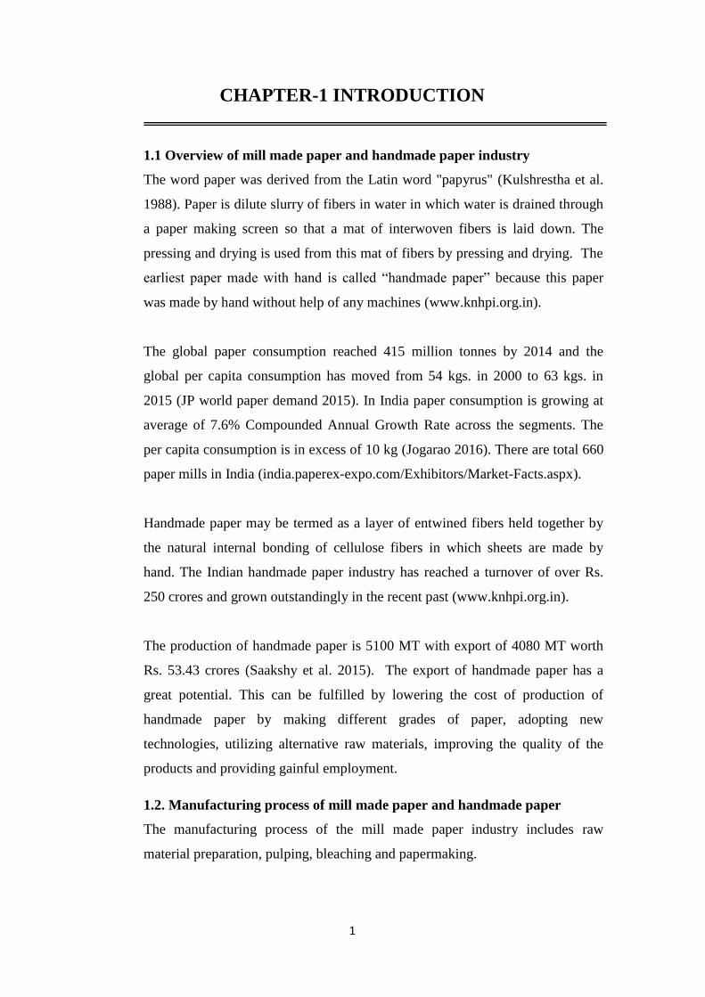
The process flow diagram of handmade paper making process using cotton rags
as raw material is given as Figure-1.1.
Figure 1.1 Process flow chart of handmade paper making process using cotton
rags as raw material (www.knhpi.org.in)
Raw material
Dusting of
cotton rags Dust
Chopping of
cotton rags
Fresh
water/Back
water Beater Wash Beating
Fresh
water/Back
water Stock chest
Fresh
water/Back
water
Sheet making
Pressing
Evaporation
Drying
Calendaring
Cutting
Packing
3
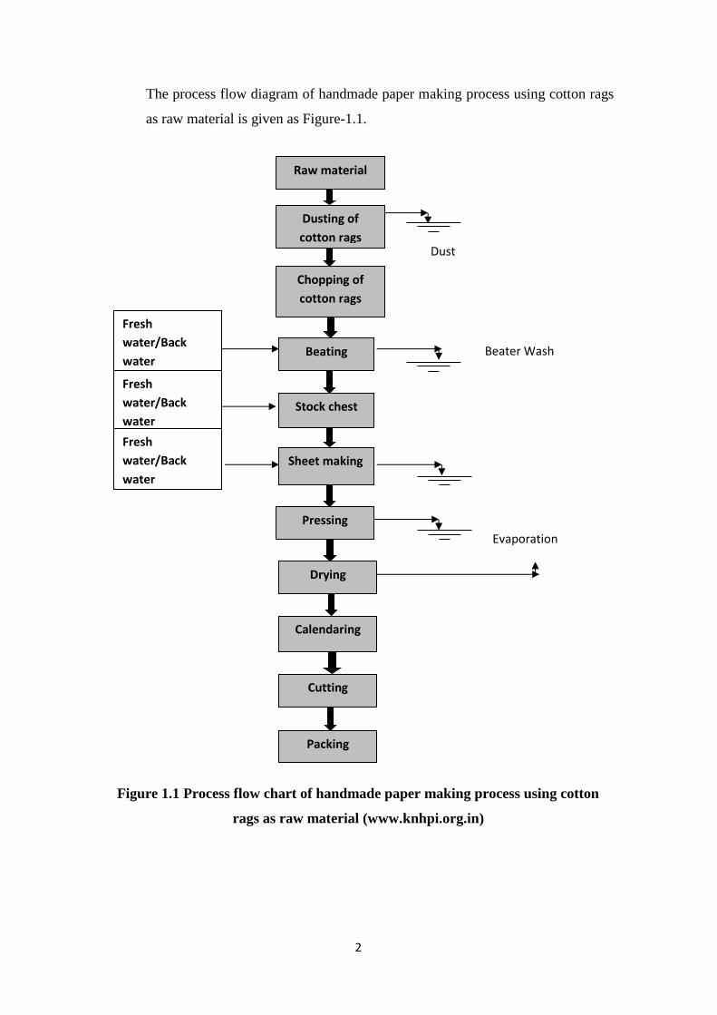
The flow chart for making paper out of alternative ligno-cellulosic raw material is given
as Figure-1.2.
Figure 1.2 Process flow chart of handmade paper making process using alternative
ligno-cellulosic raw material (www.knhpi.org.in)
Alternative Ligno-
cellulosic raw
material
Cutting of fiber
Black Liquor Digestion/Pulping Fresh
water/Back
water
Wash
Liquor Washing Fresh
water/Back
water
Beater Wash Beating Fresh
water/Back
water
Stock chest
Sheet making
Pressing
Evaporation
Drying
Calendaring
Cutting
Packing
4
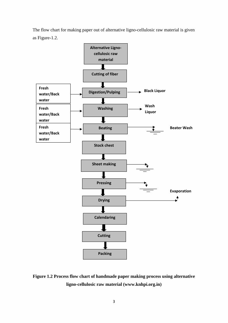
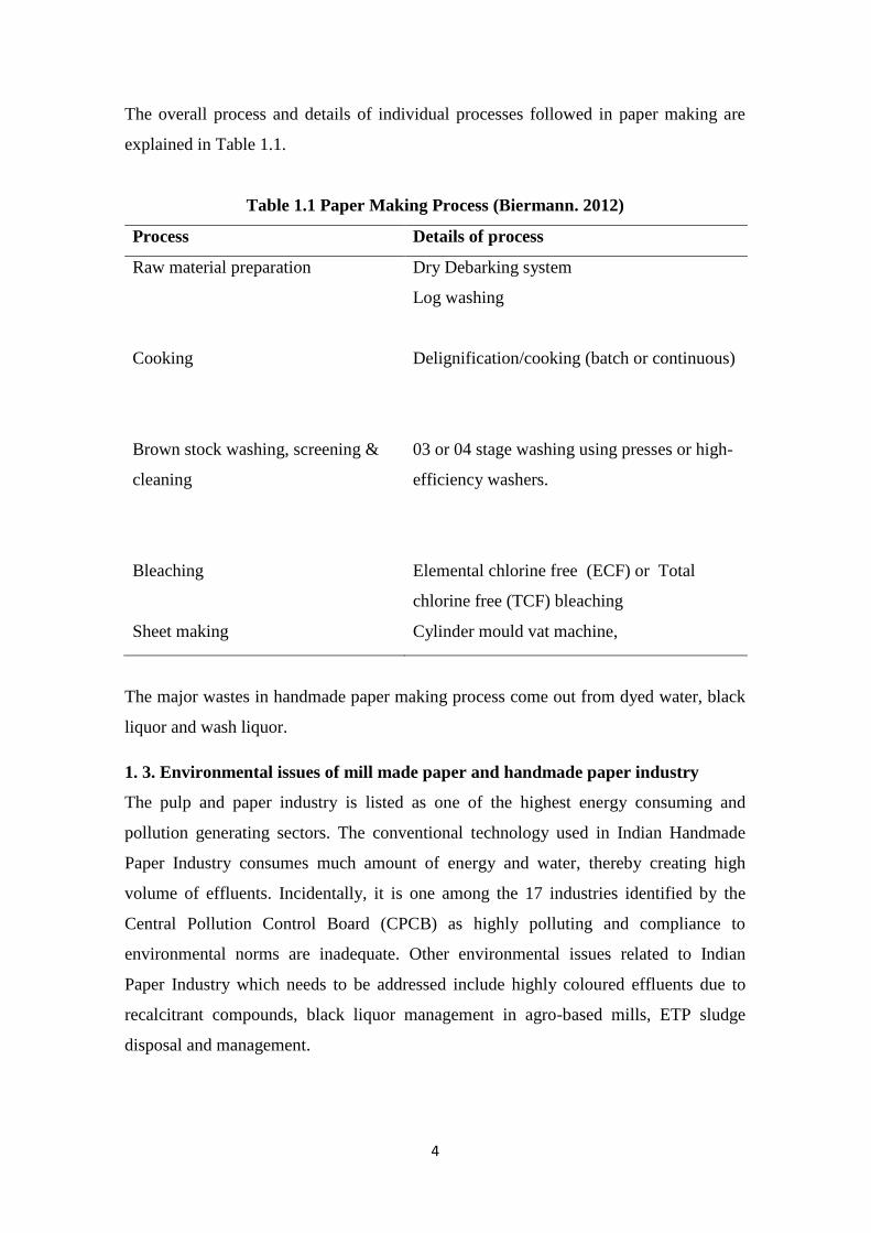
The overall process and details of individual processes followed in paper making are
explained in Table 1.1.
Table 1.1 Paper Making Process (Biermann. 2012)
Process Details of process
Raw material preparation Dry Debarking system
Log washing
Cooking Delignification/cooking (batch or continuous)
Brown stock washing, screening &
cleaning
03 or 04 stage washing using presses or high-
efficiency washers.
Bleaching Elemental chlorine free (ECF) or Total
chlorine free (TCF) bleaching
Sheet making Cylinder mould vat machine,
The major wastes in handmade paper making process come out from dyed water, black
liquor and wash liquor.
1. 3. Environmental issues of mill made paper and handmade paper industry
The pulp and paper industry is listed as one of the highest energy consuming and
pollution generating sectors. The conventional technology used in Indian Handmade
Paper Industry consumes much amount of energy and water, thereby creating high
volume of effluents. Incidentally, it is one among the 17 industries identified by the
Central Pollution Control Board (CPCB) as highly polluting and compliance to
environmental norms are inadequate. Other environmental issues related to Indian
Paper Industry which needs to be addressed include highly coloured effluents due to
recalcitrant compounds, black liquor management in agro-based mills, ETP sludge
disposal and management.
5
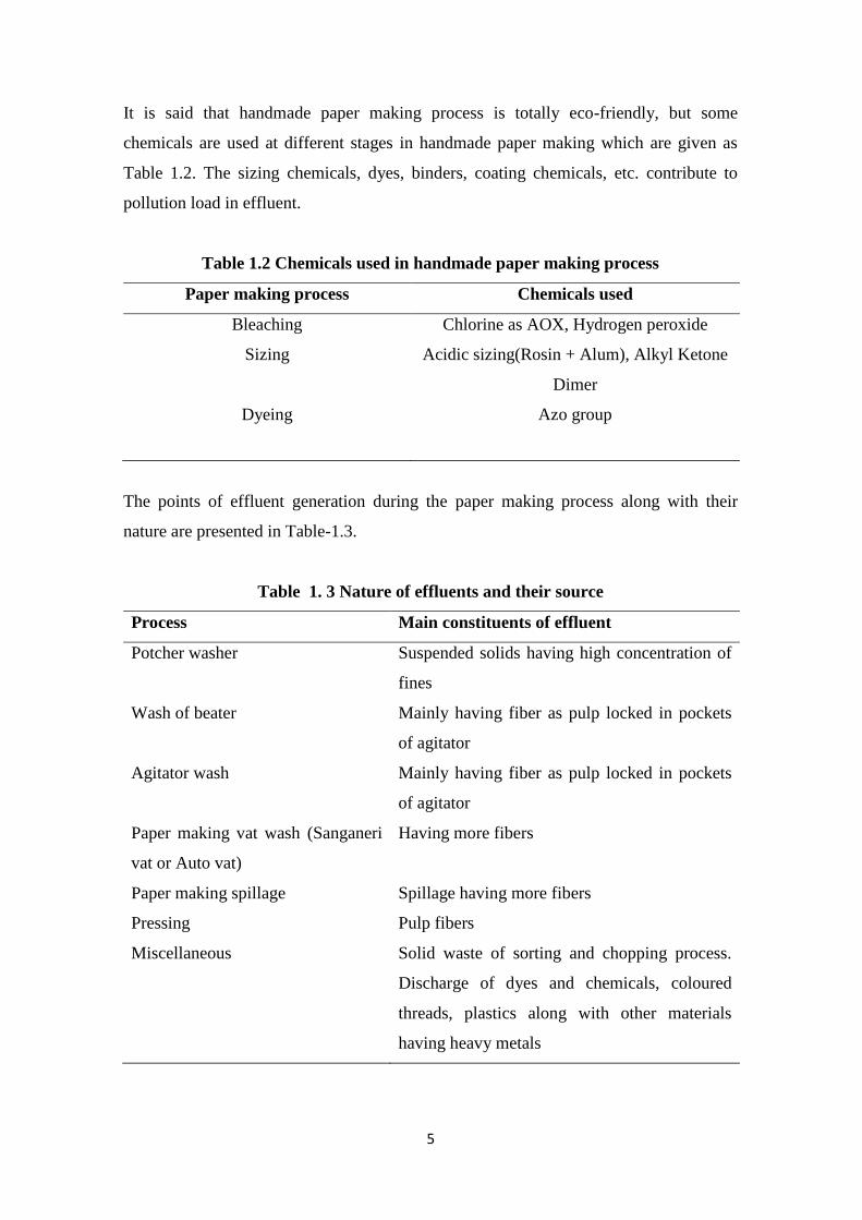
It is said that handmade paper making process is totally eco-friendly, but some
chemicals are used at different stages in handmade paper making which are given as
Table 1.2. The sizing chemicals, dyes, binders, coating chemicals, etc. contribute to
pollution load in effluent.
Table 1.2 Chemicals used in handmade paper making process
Paper making process Chemicals used
Bleaching Chlorine as AOX, Hydrogen peroxide
Sizing Acidic sizing(Rosin + Alum), Alkyl Ketone
Dimer
Dyeing Azo group
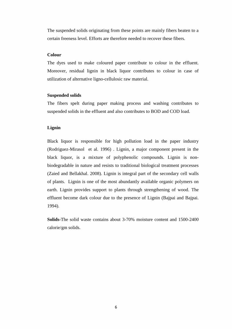
The points of effluent generation during the paper making process along with their
nature are presented in Table-1.3.
Table 1. 3 Nature of effluents and their source
Process Main constituents of effluent
Potcher washer Suspended solids having high concentration of
fines
Wash of beater Mainly having fiber as pulp locked in pockets
of agitator
Agitator wash Mainly having fiber as pulp locked in pockets
of agitator
Paper making vat wash (Sanganeri
vat or Auto vat)
Having more fibers
Paper making spillage Spillage having more fibers
Pressing Pulp fibers
Miscellaneous Solid waste of sorting and chopping process.
Discharge of dyes and chemicals, coloured
threads, plastics along with other materials
having heavy metals
6
The suspended solids originating from these points are mainly fibers beaten to a
certain freeness level. Efforts are therefore needed to recover these fibers.
Colour
The dyes used to make coloured paper contribute to colour in the effluent.
Moreover, residual lignin in black liquor contributes to colour in case of
utilization of alternative ligno-cellulosic raw material.
Suspended solids
The fibers spelt during paper making process and washing contributes to
suspended solids in the effluent and also contributes to BOD and COD load.
Lignin
Black liquor is responsible for high pollution load in the paper industry
(Rodriguez-Mirasol et al. 1996) . Lignin, a major component present in the
black liquor, is a mixture of polyphenolic compounds. Lignin is non-
biodegradable in nature and resists to traditional biological treatment processes
(Zaied and Bellakhal. 2008). Lignin is integral part of the secondary cell walls
of plants. Lignin is one of the most abundantly available organic polymers on
earth. Lignin provides support to plants through strengthening of wood. The
effluent become dark colour due to the presence of Lignin (Bajpai and Bajpai.
1994).
Solids-The solid waste contains about 3-70% moisture content and 1500-2400
calorie/gm solids.
7
1.4. Treatment techniques of effluent of mill made paper and handmade
paper industry
The treatment techniques of mill made paper differ widely with handmade paper
industry as the effluent discharged from mill made paper is more polluted than
handmade paper industry.
1.4.1 Treatment techniques of paper industry
Acid precipitation
Chemical precipitation involves separation and precipitation of lignin and other
inorganic compounds by reducing the pH of the effluent below 6.5. The
maximum precipitation occurs in the pH range of 3-4. The technique is easy but
it is expensive due to cost of chemicals. There is difficulty in handling of
precipitated sludge and difficult in separation of precipitated mass due to
hydrophilic nature of lignin.
The precipitation of lignin by acidification is one of the potential treatment of
black liquor (Loutfi et al. 1991; Davy et al. 1998; Ohman. 2006; Ohman and
Theliander. 2007) using sulfuric acid (Uloth and Wearing. 1989). The sulfuric
acid interferes in the liquor cycle chemical balance with excess sulfur
(Loutfi et al. 1991). Therefore, CO2 is preferred for acidification for black
liquor (Loutfi et al. 1991; Olsson et al. 2006). The separation of lignin from
black liquor is an important step (Ohman and Theliander. 2007). Almost 50 %
of the COD in black liquor can be removed after separation of lignin from black
liquor (Abacherli et al. 1999).
Biological treatment methods
Biological treatment method is still considered as partial successful alternative
for black liquor treatment among the treatment alternatives of black liquor. A
selected group of fungi and basidiomycete have been shown to possess
ligninolytic enzyme systems (Kirk and Cullen. 1998). The white rot fungus
Trametes versicolour was found to reduce color of black liquor and effluent
effectively (Varasavanan and Sreekrishnan. 2005).
8
Advanced oxidation
Ozonation
The ozone has a specific sharp odour and can be detected above 0.01 mg/l in air.
The ozone gas is a potential germicide and also used as an oxidizing agent.
Ozone production from pure oxygen is an appropriate and economical solution.
The ozonation treatment needs high capital investment even though the
operating cost is low. Ozone is a strong oxidant (E0 = 2.08 V). Ozone oxidizes
the complex aromatic rings of dyestuffs (Fanchiang et al. 2009). The ozone is an
unstable molecule and therefore, generated near the site. Ozonation does not
yield complete mineralization to CO2 and H2O (Assalin et al. 2004)
Chemical coagulation
The chemical coagulation is widely used for wastewater treatment. It is an
integral treatment step in the surface or underground water treatment. The most
widely used chemicals for chemical coagulation include aluminum chloride,
ferric chloride, barium chloride and copper sulphate (Ukiwe et al. 2014)
Adsorption
The adsorption method is effective in removal of trace component from the
wastewater. There are various adsorbents including activated carbon, zeolite,
charcoal, fly ash etc. for adsorption applications. The fly ash is fine mineral
residue collected in electrostatic precipitators collected after the combustion of
coal in electricity generating plant. Fly ash is usually slit shaped with size 0.005-
–0.074 mm (Heidrich et al. 2013).
1.4.2 Treatment techniques for the effluent of handmade paper industry
In the present scenario, the Indian handmade paper industry normally does not
use any treatment techniques and discharge as such without any treatment as this
is a small scale industry. Handmade paper industries use direct dyes to make
brilliant coloured paper, which is used in making fancy and decorative papers,
wedding cards, stationery items etc. These industries use negligible chemicals
but due to abundant use of direct dye, the main component in effluent is dye.
9
The handmade paper industry is a small scale industry and cannot afford the
costly or complex wastewater treatment technologies. The low cost fly ash can
offer a cost effective technology for handmade paper sector.
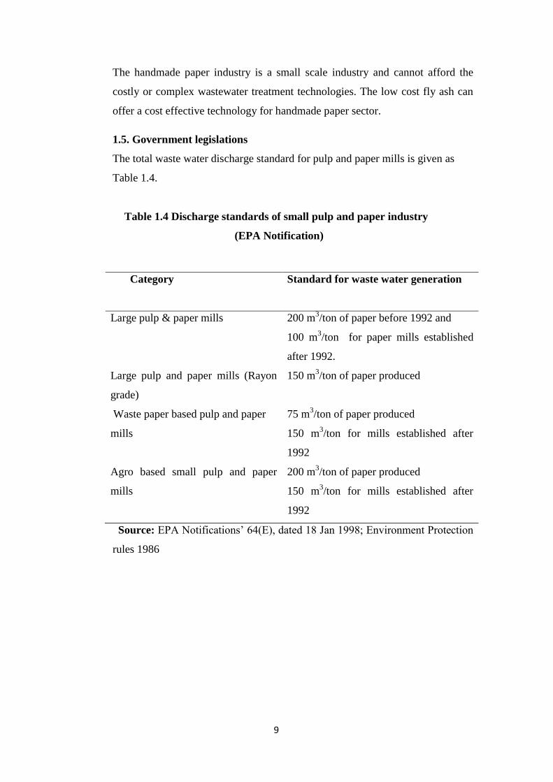
1.5. Government legislations
The total waste water discharge standard for pulp and paper mills is given as
Table 1.4.
Table 1.4 Discharge standards of small pulp and paper industry
(EPA Notification)
Category
Standard for waste water generation
Large pulp & paper mills 200 m3/ton of paper before 1992 and
100 m3/ton for paper mills established
after 1992.
Large pulp and paper mills (Rayon
grade)
150 m3/ton of paper produced
Waste paper based pulp and paper
mills
75 m3/ton of paper produced
150 m3/ton for mills established after
1992
Agro based small pulp and paper
mills
200 m3/ton of paper produced
150 m3/ton for mills established after
1992
Source: EPA Notifications’ 64(E), dated 18 Jan 1998; Environment Protection
rules 1986
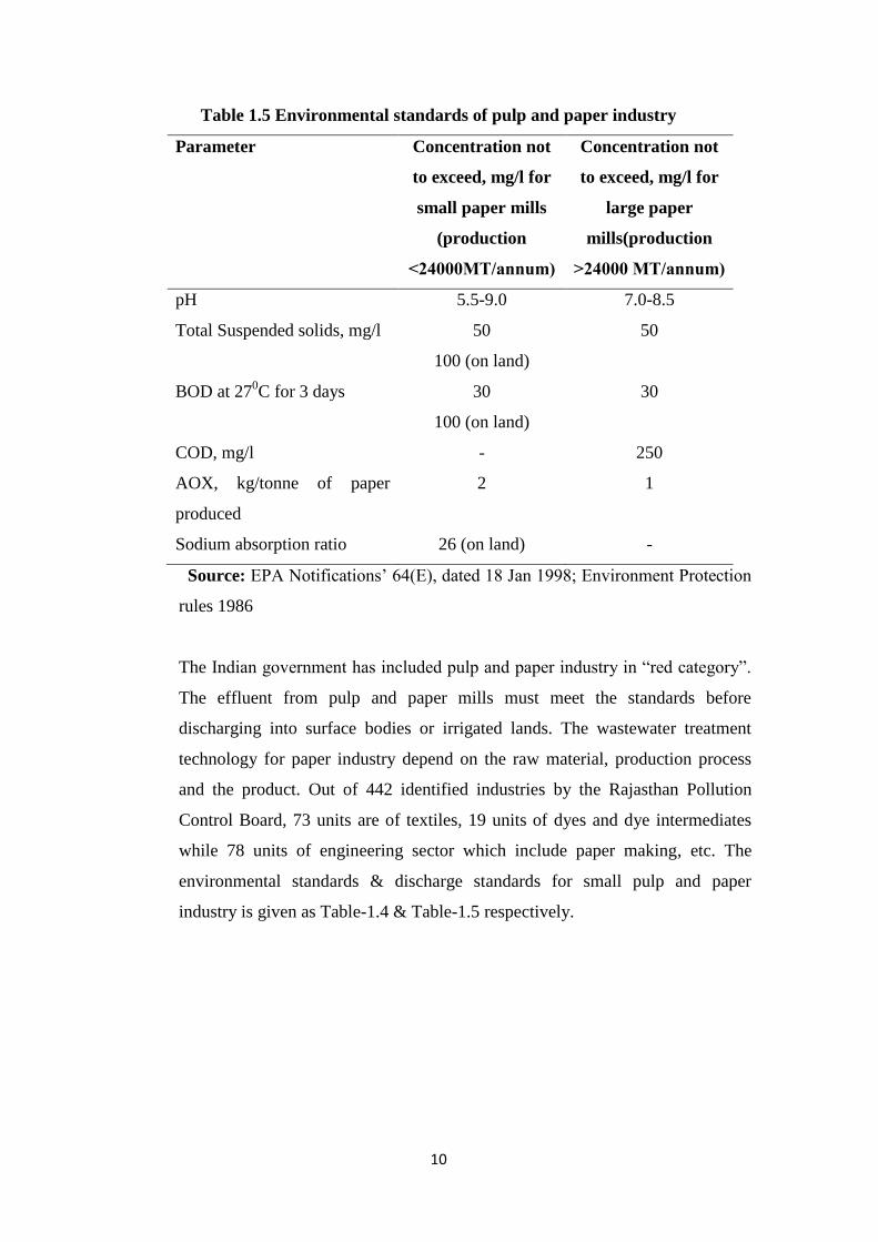
10
Table 1.5 Environmental standards of pulp and paper industry
Parameter Concentration not
to exceed, mg/l for
small paper mills
(production
˂24000MT/annum)
Concentration not
to exceed, mg/l for
large paper
mills(production
˃24000 MT/annum)
pH 5.5-9.0 7.0-8.5
Total Suspended solids, mg/l 50
100 (on land)
50
BOD at 270C for 3 days 30
100 (on land)
30
COD, mg/l - 250
AOX, kg/tonne of paper
produced
2 1
Sodium absorption ratio 26 (on land) -
Source: EPA Notifications’ 64(E), dated 18 Jan 1998; Environment Protection
rules 1986
The Indian government has included pulp and paper industry in “red category”.
The effluent from pulp and paper mills must meet the standards before
discharging into surface bodies or irrigated lands. The wastewater treatment
technology for paper industry depend on the raw material, production process
and the product. Out of 442 identified industries by the Rajasthan Pollution
Control Board, 73 units are of textiles, 19 units of dyes and dye intermediates
while 78 units of engineering sector which include paper making, etc. The
environmental standards & discharge standards for small pulp and paper
industry is given as Table-1.4 & Table-1.5 respectively.
11
1.6 Origin and significance of the present study
In the present scenario, the physical and biological treatment system are not
found adequate enough for the wastewater to meet the prescribed effluent norms
and for waste water recycling within the existing process. Therefore, tertiary
treatment is the requirement (Charter, Central Pollution Control Board, 2015).
Handmade paper industry is using cotton hosiery and alternative ligno-cellulosic
as raw material. The process consumes huge amount of water and goes as waste
without any recovery. In the present day context, handmade paper units are also
facing water shortage as the groundwater level is going down day by day and
therefore minimization of water utilization and recycling of treated water using
simple treatment methods is needed to conserve handmade paper making
community. Therefore there is a need to make a detailed study and emphasize
on recycling of water in handmade paper sector in order to make it eco-friendly.
Previously, the handmade paper industry was kept by the Central Pollution
Control Board in green category and no objection certificate was issued to
handmade paper units being classified under small scale sector. Now they have
shifted handmade paper industry to orange category. As Sanganer is a cluster of
handmade paper industries, it is essential for them to treat the effluent at
affordable and easy to operate technology.
1.7 Objectives of the study
The broad objective of this research work is to closely examine the processes
that generate effluent in a typical handmade paper industry and devise a suitable
techno-managerial strategy for its safe disposal, which can be handled at small
scale industry level. The specific objectives of the research work are:
To devise a suitable strategy for waste minimization.
Characterization of effluent streams from handmade paper industry and
assessment of possible reduction in water consumption by way of
recycling and reuse of partially/ completely treated effluents.
12
Treatment of major effluent streams through low cost adsorption using
fly ash, understanding the mechanism of sorption, and reuse of spent
adsorbent for a possible close loop operation.
Treatment of major effluent streams through biological/ chemical
oxidation; mathematical modelling and simulation for developing kinetic
parameters for the design of such systems; and utilization of sludge
generated from the process.
1.8 Scope of work
The scope of the research work is as given below:
Quantitative assessment, Characterization of different streams of effluent
discharged from different operations of handmade paper making
synthetic wastewater using conventional and alternative ligno-cellulosic
raw material to minimize the waste emission.
Feasibility studies following different treatment methods in sequence
including adsorption, ozonation, bacteria, fungi etc. of effluent of
conventional raw material and black liquor of different alternative ligno-
cellulosic raw material.
Trial to mix this with some organic solid waste to develop high energy
briquettes/compost.
Treatment kinetics for treatment of effluent.
Development of mathematical model and model validation by
experimental data.
1.9 Organization of the thesis
This thesis is organized in to ten chapters. Chapter 1 consists of introduction and
objectives of the study. Chapter 2 compiles literature related to the waste water
treatment methods for paper industry. The topics included in Chapter 3 describe
details of the material and methods adopted for conducting studies while those
included in Chapter 4 present the details of experimental setup for waste water
treatment studies. The characterization studies are included in Chapter 5. The
details of adsorption studies with fly ash as adsorbent are included in Chapter 6
and details of ozonation studies for treatment of waste water treatment are given
in Chapter 7.

13
The Chapter 8 includes microbiological studies for black liquor and Chapter 9
consists of details of utilization of sludge of handmade paper industry to make
energy briquettes. Chapter 10 includes the conclusion of this study.
14
CHAPTER 2 LITERATURE REVIEW
2.1 Introduction of paper making
In India, the history of papermaking dates back to the 3rd
century BC. The
handmade paper making has been practiced by a “Kagzis” for generations
together (Saakshy et al. 2013). Even in the 14th
century, during the rule of
Feroze Shah Tughlaq, the royal family used handmade paper for official
documents, miniature paintings, calligraphy to make copies of the Holy Quran
and to maintain account books. In the 16th
century, the ruler of Amber, Raja
Man Singh brought the Kagzis to Sanganer (www.knhpi.org.in).
Approximately, 400 million metric tons per annum of paper and cardboard are
produced globally. The China alone is responsible for around one quarter of the
total production (Bajpai 2016; www.statistica.com). The United States, Japan,
Germany, Canada, China, Finland, republic of Korea, Indonesia, Sweden and
Brazil are the world’s largest paper and paperboard producers. The largest pulp
producers are United States, China, Canada, Brazil, Sweden, Finland, Japan,
Russian Federation, Indonesia and Chile. These countries together were
responsible for 81% and 73% of the world’s pulp and paper and paperboard
production in 2010 respectively (FAO 2014; Fracaro et al. 2012;
www.fao.org/forestry/statistics;www.paperindustryworld.com;www.ibisworld.c
om/industry/global/global-paper-pulp-mills.html).
2.2 Raw Material
The raw material used in paper industry and handmade paper industry differ
widely as low lignin raw material is used in the handmade paper industry.
2.2.1 Raw material used in Indian paper industry
The major raw material used in the Indian paper industry is broadly categorized
as hardwoods, softwoods and recycled fiber.
15
The consumption of wood as raw material is on average 9 metric tons per
annum. Wood consists of approximately 50-55% cellulose, 25-30% lignin and
20-25% hemicellulose. The hard wood species as raw material for paper
industry include poplar, casuarina, subabul, eucalyptus etc. The three categories
of non-wood fibers are used in paper industry viz. crops (hemp, kenaf, flax and
jute), agricultural residues (wheat straw, rice straw, bagasse), wild plants
(grasses, bamboo, seawood). The pre-consumer recycled fiber includes shaving,
trimmings of paper machine such as printer rejects etc. The post-consumer
recycled fiber include old waste paper collected from consumers such as
newsprint, duplex board, Kraft paper etc. (Report 2014, Govt. of India).
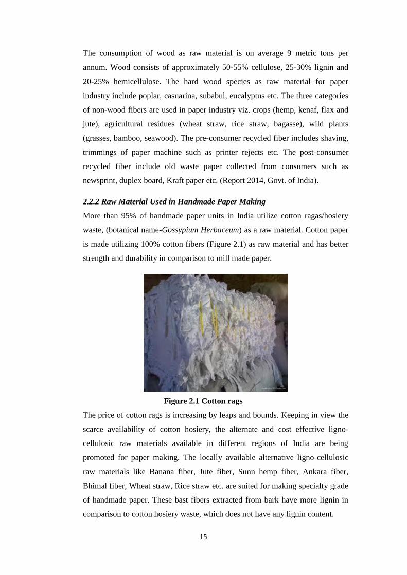
2.2.2 Raw Material Used in Handmade Paper Making
More than 95% of handmade paper units in India utilize cotton ragas/hosiery
waste, (botanical name-Gossypium Herbaceum) as a raw material. Cotton paper
is made utilizing 100% cotton fibers (Figure 2.1) as raw material and has better
strength and durability in comparison to mill made paper.
Figure 2.1 Cotton rags
The price of cotton rags is increasing by leaps and bounds. Keeping in view the
scarce availability of cotton hosiery, the alternate and cost effective ligno-
cellulosic raw materials available in different regions of India are being
promoted for paper making. The locally available alternative ligno-cellulosic
raw materials like Banana fiber, Jute fiber, Sunn hemp fiber, Ankara fiber,
Bhimal fiber, Wheat straw, Rice straw etc. are suited for making specialty grade
of handmade paper. These bast fibers extracted from bark have more lignin in
comparison to cotton hosiery waste, which does not have any lignin content.
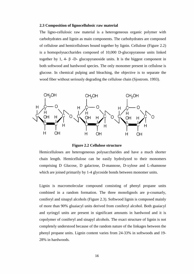
16
2.3 Composition of lignocellulosic raw material
The ligno-cellulosic raw material is a heterogeneous organic polymer with
carbohydrates and lignin as main components. The carbohydrates are composed
of cellulose and hemicelluloses bound together by lignin. Cellulose (Figure 2.2)
is a homopolysaccharides composed of 10,000 D-glucopyranose units linked
together by 1, 4- β -D- glucopyranoside units. It is the biggest component in
both softwood and hardwood species. The only monomer present in cellulose is
glucose. In chemical pulping and bleaching, the objective is to separate the
wood fiber without seriously degrading the cellulose chain (Sjostrom. 1993).
Figure 2.2 Cellulose structure
Hemicelluloses are heterogeneous polysaccharides and have a much shorter
chain length. Hemicellulose can be easily hydrolyzed to their monomers
comprising D Glucose, D galactose, D-mannose, D-xylose and L-rhamnose
which are joined primarily by 1-4 glycoside bonds between monomer units.
Lignin is macromolecular compound consisting of phenyl propane units
combined in a random formation. The three monolignols are p-coumarly,
coniferyl and sinapyl alcohols (Figure 2.3). Softwood lignin is composed mainly
of more than 90% gluaiacyl units derived from coniferyl alcohol. Both guaiacyl
and syringyl units are present in significant amounts in hardwood and it is
copolymer of coniferyl and sinapyl alcohols. The exact structure of lignin is not
completely understood because of the random nature of the linkages between the
phenyl propane units. Lignin content varies from 24-33% in softwoods and 19-
28% in hardwoods.
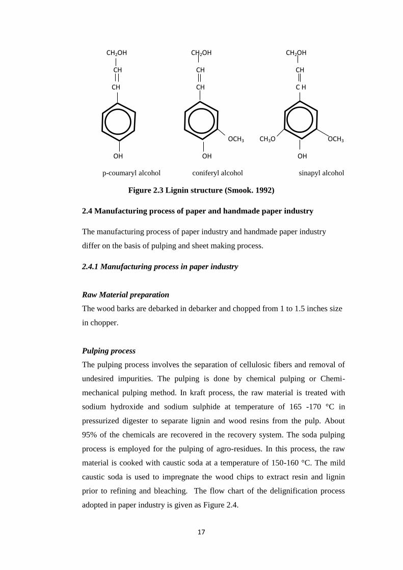
17
CH2OH CH2OH CH2OH
CH CH CH
CH CH C H
OCH3 CH3O OCH3
OH OH OH
p-coumaryl alcohol coniferyl alcohol sinapyl alcohol
Figure 2.3 Lignin structure (Smook. 1992)
2.4 Manufacturing process of paper and handmade paper industry
The manufacturing process of paper industry and handmade paper industry
differ on the basis of pulping and sheet making process.
2.4.1 Manufacturing process in paper industry
Raw Material preparation
The wood barks are debarked in debarker and chopped from 1 to 1.5 inches size
in chopper.
Pulping process
The pulping process involves the separation of cellulosic fibers and removal of
undesired impurities. The pulping is done by chemical pulping or Chemi-
mechanical pulping method. In kraft process, the raw material is treated with
sodium hydroxide and sodium sulphide at temperature of 165 -170 °C in
pressurized digester to separate lignin and wood resins from the pulp. About
95% of the chemicals are recovered in the recovery system. The soda pulping
process is employed for the pulping of agro-residues. In this process, the raw
material is cooked with caustic soda at a temperature of 150-160 °C. The mild
caustic soda is used to impregnate the wood chips to extract resin and lignin
prior to refining and bleaching. The flow chart of the delignification process
adopted in paper industry is given as Figure 2.4.
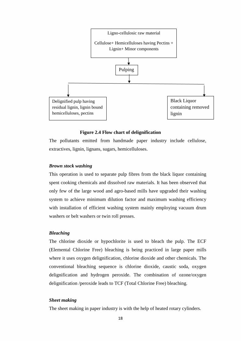
18
Figure 2.4 Flow chart of delignification
The pollutants emitted from handmade paper industry include cellulose,
extractives, lignin, lignans, sugars, hemicelluloses.
Brown stock washing
This operation is used to separate pulp fibres from the black liquor containing
spent cooking chemicals and dissolved raw materials. It has been observed that
only few of the large wood and agro-based mills have upgraded their washing
system to achieve minimum dilution factor and maximum washing efficiency
with installation of efficient washing system mainly employing vacuum drum
washers or belt washers or twin roll presses.
Bleaching
The chlorine dioxide or hypochlorite is used to bleach the pulp. The ECF
(Elemental Chlorine Free) bleaching is being practiced in large paper mills
where it uses oxygen delignification, chlorine dioxide and other chemicals. The
conventional bleaching sequence is chlorine dioxide, caustic soda, oxygen
delignification and hydrogen peroxide. The combination of ozone/oxygen
delignification /peroxide leads to TCF (Total Chlorine Free) bleaching.
Sheet making
The sheet making in paper industry is with the help of heated rotary cylinders.
Ligno-cellulosic raw material
Cellulose+ Hemicelluloses having Pectins +
Lignin+ Minor components
Pulping
Delignified pulp having
residual lignin, lignin bound
hemicelluloses, pectins
Black Liquor
containing removed
lignin
19
2.4.2 Manufacturing process in handmade paper industry
The raw material is vigorously shaken to remove the dust and dirt and then
sorted manually to remove extraneous materials. The sorted material is chopped
to 1 to 1.5 inches. The chopped raw material in case of cotton rags is fed in
beater along with water and beaten in a Hollander beater. The handmade paper
sheets are formed with diluted pulp slurry in a vat. The lifting mould is dipped
into the vat, shaken vigorously and lifted out with the layer of entwined fibres
on the mould. The sheets are made with the help of a cylinder mould vat
machine and sanganeri vats. Then, wet paper is transferred onto a cotton cloth
or felt. A hydraulic press or pneumatic press is used to remove the excess water
from the sheets. The sheets are dried by hanging them in an covered area or
under sunlight for drying. The dried sheets are placed between metallic plates
and passed through heavy rollers in a calendaring machine for smoothening of
paper sheets. The sheets are then cut to the desired size using a cutting machine
or guillotine cutter.
2.5 Environmental issues
The environmental issues of paper industry and handmade paper industry are
presented here.
2.5.1 Emission issues for paper industry
The pulp and paper industry is the third largest consumer of fresh water with
consumption in the range 80-150 m3/t of paper (GOI, 2014). Generally agro
based mills consume much more water than Recycled Fiber based mills. The
waste water discharged from paper industry contains various chemicals like
thiols, sulphur dioxide, sulphite and sulphides, fibres and resins; bleaching
agents and whitening agents. The effluent of paper industry constitutes of
organic pollutants (starch, fibers, hemicellulose, and organic (acids). The
composition of the black liquor depends on the raw material and the production
process and varies considerably between different mills (Smook, 1992). The
phenolic compounds present in black liquor pose powerful toxic effect on
microorganisms.
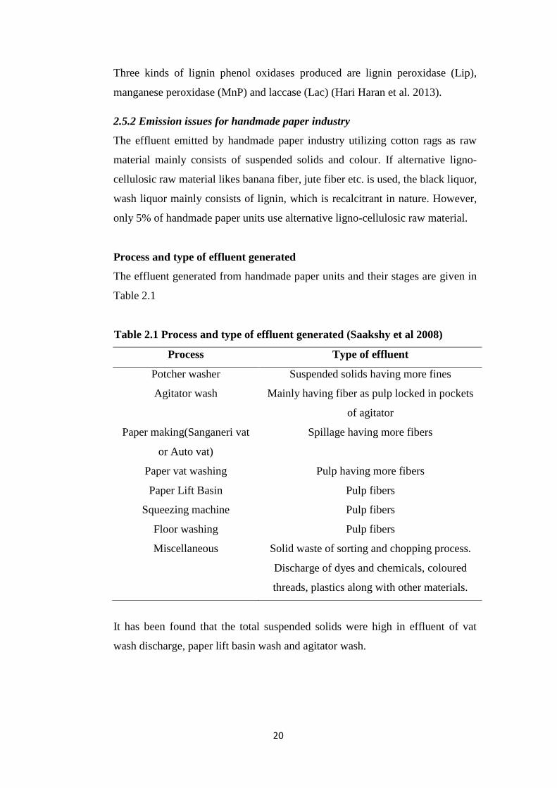
20
Three kinds of lignin phenol oxidases produced are lignin peroxidase (Lip),
manganese peroxidase (MnP) and laccase (Lac) (Hari Haran et al. 2013).
2.5.2 Emission issues for handmade paper industry
The effluent emitted by handmade paper industry utilizing cotton rags as raw
material mainly consists of suspended solids and colour. If alternative ligno-
cellulosic raw material likes banana fiber, jute fiber etc. is used, the black liquor,
wash liquor mainly consists of lignin, which is recalcitrant in nature. However,
only 5% of handmade paper units use alternative ligno-cellulosic raw material.
Process and type of effluent generated
The effluent generated from handmade paper units and their stages are given in
Table 2.1
Table 2.1 Process and type of effluent generated (Saakshy et al 2008)
Process Type of effluent
Potcher washer Suspended solids having more fines
Agitator wash Mainly having fiber as pulp locked in pockets
of agitator
Paper making(Sanganeri vat
or Auto vat)
Spillage having more fibers
Paper vat washing Pulp having more fibers
Paper Lift Basin Pulp fibers
Squeezing machine Pulp fibers
Floor washing Pulp fibers
Miscellaneous Solid waste of sorting and chopping process.
Discharge of dyes and chemicals, coloured
threads, plastics along with other materials.
It has been found that the total suspended solids were high in effluent of vat
wash discharge, paper lift basin wash and agitator wash.
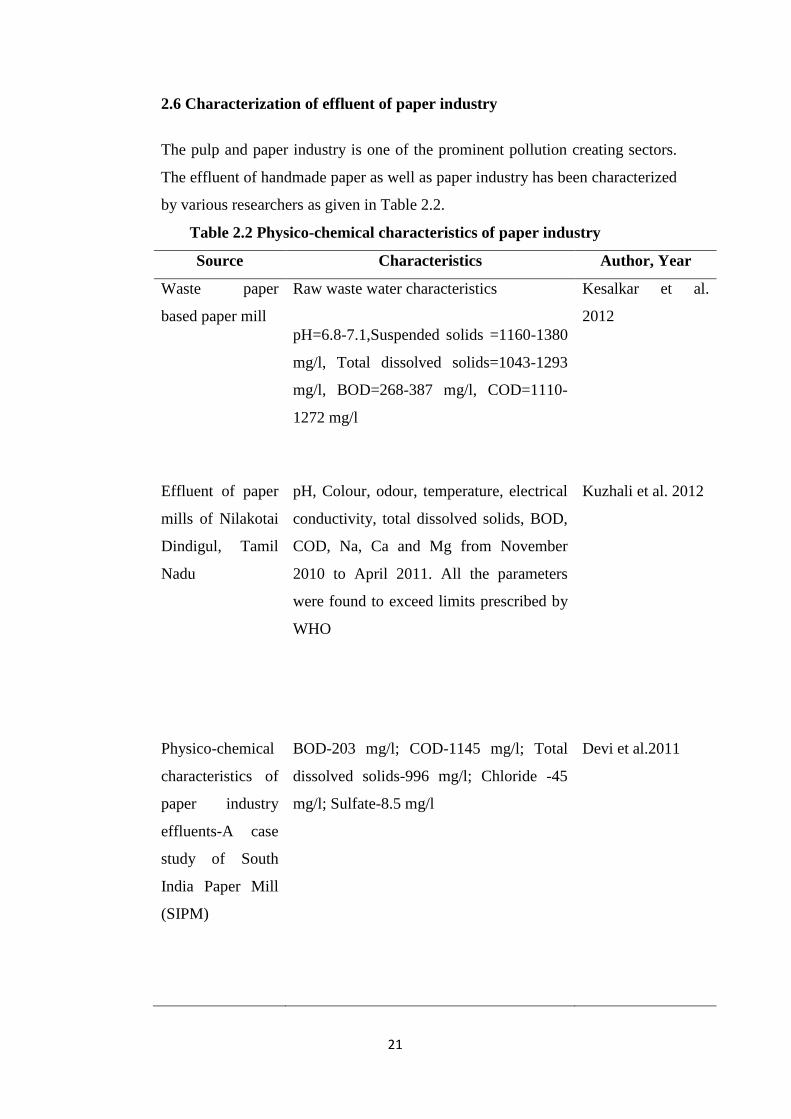
21
2.6 Characterization of effluent of paper industry
The pulp and paper industry is one of the prominent pollution creating sectors.
The effluent of handmade paper as well as paper industry has been characterized
by various researchers as given in Table 2.2.
Table 2.2 Physico-chemical characteristics of paper industry
Source Characteristics Author, Year
Waste paper
based paper mill
Raw waste water characteristics
pH=6.8-7.1,Suspended solids =1160-1380
mg/l, Total dissolved solids=1043-1293
mg/l, BOD=268-387 mg/l, COD=1110-
1272 mg/l
Kesalkar et al.
2012
Effluent of paper
mills of Nilakotai
Dindigul, Tamil
Nadu
pH, Colour, odour, temperature, electrical
conductivity, total dissolved solids, BOD,
COD, Na, Ca and Mg from November
2010 to April 2011. All the parameters
were found to exceed limits prescribed by
WHO
Kuzhali et al. 2012
Physico-chemical
characteristics of
paper industry
effluents-A case
study of South
India Paper Mill
(SIPM)
BOD-203 mg/l; COD-1145 mg/l; Total
dissolved solids-996 mg/l; Chloride -45
mg/l; Sulfate-8.5 mg/l
Devi et al.2011
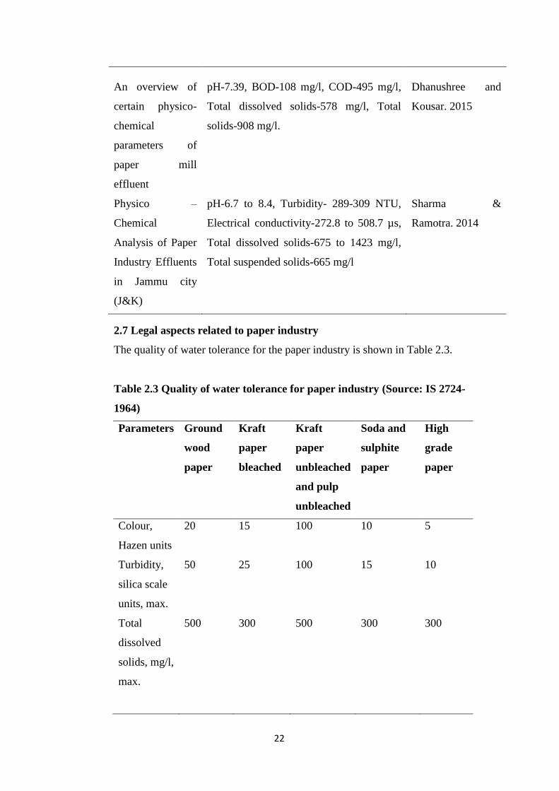
22
An overview of
certain physico-
chemical
parameters of
paper mill
effluent
pH-7.39, BOD-108 mg/l, COD-495 mg/l,
Total dissolved solids-578 mg/l, Total
solids-908 mg/l.
Dhanushree and
Kousar. 2015
Physico –
Chemical
Analysis of Paper
Industry Effluents
in Jammu city
(J&K)
pH-6.7 to 8.4, Turbidity- 289-309 NTU,
Electrical conductivity-272.8 to 508.7 µs,
Total dissolved solids-675 to 1423 mg/l,
Total suspended solids-665 mg/l
Sharma &
Ramotra. 2014
2.7 Legal aspects related to paper industry
The quality of water tolerance for the paper industry is shown in Table 2.3.
Table 2.3 Quality of water tolerance for paper industry (Source: IS 2724-
1964)
Parameters Ground
wood
paper
Kraft
paper
bleached
Kraft
paper
unbleached
and pulp
unbleached
Soda and
sulphite
paper
High
grade
paper
Colour,
Hazen units
20 15 100 10 5
Turbidity,
silica scale
units, max.
50 25 100 15 10
Total
dissolved
solids, mg/l,
max.
500 300 500 300 300
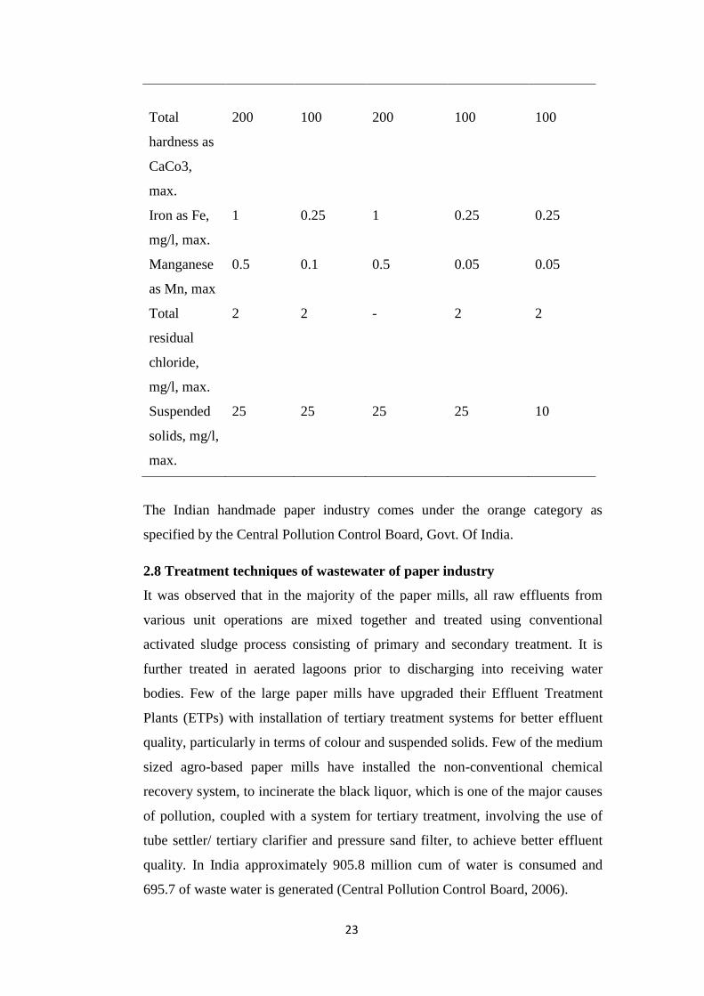
23
Total
hardness as
CaCo3,
max.
200 100 200 100 100
Iron as Fe,
mg/l, max.
1 0.25 1 0.25 0.25
Manganese
as Mn, max
0.5 0.1 0.5 0.05 0.05
Total
residual
chloride,
mg/l, max.
2 2 - 2 2
Suspended
solids, mg/l,
max.
25 25 25 25 10
The Indian handmade paper industry comes under the orange category as
specified by the Central Pollution Control Board, Govt. Of India.
2.8 Treatment techniques of wastewater of paper industry
It was observed that in the majority of the paper mills, all raw effluents from
various unit operations are mixed together and treated using conventional
activated sludge process consisting of primary and secondary treatment. It is
further treated in aerated lagoons prior to discharging into receiving water
bodies. Few of the large paper mills have upgraded their Effluent Treatment
Plants (ETPs) with installation of tertiary treatment systems for better effluent
quality, particularly in terms of colour and suspended solids. Few of the medium
sized agro-based paper mills have installed the non-conventional chemical
recovery system, to incinerate the black liquor, which is one of the major causes
of pollution, coupled with a system for tertiary treatment, involving the use of
tube settler/ tertiary clarifier and pressure sand filter, to achieve better effluent
quality. In India approximately 905.8 million cum of water is consumed and
695.7 of waste water is generated (Central Pollution Control Board, 2006).
24
The water consumption by agro industries making writing and printing paper,
kraft paper mills is reported to consume 100 m3/T and 75 m
3/T respectively. The
recycled fiber based industry making writing and printing paper, duplex board,
newsprint consume 50 m3 /T while kraft paper mills consume 35 m
3/T of water.
2.8.1 Chemical precipitation
Studies have been conducted with aluminum chloride, ferric chloride, barium
chloride and copper sulphate for chemical precipitation of paper industry
effluent. The aluminum chloride dosage of 4 g/l showed 99.8% of colour
removal at pH-5.0. The ferric chloride showed 99% colour removal at 4 pH and
dosage of 2 g/l.
The copper sulphate was quite effective at pH-10 removing
colour up to 96%, phenols 94%, TSS 94%, at a dosage of 2.5 g/l. The barium
chloride showed 96% colour removal at 9-12 pH (Swamy et al. 2016). A 5 g/l of
dosage of aluminium chloride gave 86.30 % colour removal, copper sulphate as
coagulant could remove 74% COD, polyaluminium chloride could give 82.85%
COD removal and 91.81% colour removal in another study (Kumar et al.
2011).
Poly aluminium chloride dosage of 8 ml/L reduced COD and colour by 83% and
92% respectively at pH- 5.0. The 72% COD and 84% colour removal were
observed with AlCl3 dosage of 5 g/l at pH-4.0 (Chaudhary et al 2010).
2.8.2 Adsorption
The adsorption process for the treatment of paper effluent is generally physical
in nature resulting from the effect of Van der Waals forces. On the other hand,
chemisorption involves the exchange or sharing of electrons. The adsorbent
should have large surface area and should be mechanically strong.
2.8.3 Ozonation
The ozonation treatment is known to be effective for decomposing organic
chemicals containing C=C bonds, aromatic compounds, phenols, polycyclic
aromatics, heterocyclics, C=N and C-H bonds. The ozone does not increase the
volume of wastewater and sludge and can be applied in its gaseous state
(Sundrarajan et al., 2007).
25
2.9 Adsorption isotherms
2.9.1 Langmuir Isotherms
The Langmuir adsorption isotherm assumes that adsorption occurs at specific
homogeneous sites and occurs as monolayer adsorption. The Langmuir equation
in linear form is given as equation 2.1:
maxmax
1
q
C
Kqq
C e
Le
e ………………………………………………….(Eq. 2. 1)
The values of qmax and KL were computed from the slope and intercept of the
graph between Ce/qe with respect to Ce. .The Langmuir isotherm can be given by
separation or equilibrium parameter given by equation 2.2:
01
1
CKR
L
L
………………………………………………………... (Eq. 2.2)
RL indicates the type of isotherms (Vijayaraghavan et al., 2006; Kundu and
Gupta, 2006; Pérez-Marín et al., 2007; Webber and Chakravorti, 1974). The RL
values between zero and one confirms the favorable uptake of adsorbate on
adsorbent.
2.9.2 Freundlich isotherm
Freundlich isotherm is based on non -uniform and non-ideal reversible
adsorption over heterogeneous surfaces that are not limited to the formation of
the monolayer adsorption (Bajeer et al., 2012; Freundlich, 1906; Adamson and
Gast, 1997). A linear form of Freundlich expression is obtained by taking
logarithm as shown in equation 2.3:
efe Cn
Kq ln1
lnln ………………………………………………..(Eq. 2.3)
The plot of ln qe versus ln Ce gives the value of Kf and 1/n. The graph between
ln qe with respect to ln Ce gives the value of 1/n and Kf.
26
2.9.3 Temkin isotherm
Temkin isotherm takes into the account of adsorbent–adsorbate interaction
(Temkin and Pyzhev, 1940; Aharoni and Ungarish, 1977) is given by the
equation 2.4:
eTTTe CBABq lnln ………………………………………………(Eq. 2.4)
A plot of qe versus ln Ce enables the determination of isotherm constants Kt and
B1.
2.10 Kinetic models of adsorption
The three models pseudo first order, pseudo second order rate equation and
intra-particle diffusion model was studied.
2.10.1 Pseudo first order kinetic model
Lagergren equation is given to study pseudo first order kinetic model.
303.2
loglog 1tkqqq ete ……………………………………….(Eq. 2.5)
The value of k1 is evaluated by the slope of the graph between log (qe-qt) and
time at different concentration. The values of k1 and qe are calculated from the
slope and intercept of the graph.
2.10.2 Pseudo-Second order kinetic model
The second order kinetic model is given as:
eq
t
qekq
t
2
2
1 …………………………………………………..(Eq. 2.6)
The initial adsorption rate is given as:
2
2qekh …………………………………………………..………(Eq. 2.7)
The values of h (mg/g/ min) can be calculated from the slope and intercept of
the plot t/q vs. t.
27
2.10.3 Intraparticle diffusion
In intraparticle diffusion, the uptake varies almost proportionately with the half-
power of time (Ho and McKay, 1998). The intraparticle diffusion model
proposed by Weber and Morris is given as equation 2.8:
Ctkq idt 5.0 ………………………………………………….………(Eq. 2.8)
2.11 Conventional adsorbent
Mari et al. 2006 (FPRDI) studied the treatment of wastewater from a HMP mill
of Philippines. Specifically, the study assessed the potential of a charcoal-based
treatment system in treating handmade paper mill wastewater.
The effluent was passed through settling ponds and the supernatant liquid was
fed through two aerated charcoal bed (ACBs) for about 5 days each, which
reduced biochemical oxygen demand (BOD) and total suspended solids (TSS) to
acceptable limits (www.agris. fao.org) The study was conducted to remove
colour from effluent of paper industry using waste sludge from ETP as an
adsorbent (Chakradhar et al 2004). Activated carbon is the commonly used as
an adsorbent, the major drawback being the high cost (Varma et al., 2013).
2.12 Low cost adsorbents
Coal currently caters around 42% of global electricity generation (International
Energy Agency, 2010). The thermal power generation which accounts for 80-
85% in India is expected to grow by 5% per annum. There are 88 thermal power
stations based on coal/lignite for power generation having a total installed
capacity of 80458 MW (Central Electricity Authority, 2015). The coal
consumed by these power plants during 2010-12 was 407.61 MT with total ash
generation of 131.09 MT. The generation of fly ash is expected to grow to 300-
400 MT by 2016 (www.flyash2012missionenergy.org). The annual production
of fly ash from coal power plants is 112 MT (Dhadse et al., 2008). In India,
only 3% of fly ash produced is utilized while 80% of fly ash is reused in
Germany (Senapati, 2011).
28
The Government of India focused efforts led by Fly Ash Mission (FAM),
Technology Information, Forecasting & Assessment Council (TIFAC), along
with other stakeholder agencies in 1994 for gainful utilization and safe disposal
of fly ash.
The national thermal power corporation has also taken initiatives to make good
quality of fly ash available to users. The major constituents of most of the fly
ashes are Silica (SiO2), alumina (Al2O3), ferric oxide (Fe2O3) and calcium oxide
(CaO). The other minor constituents of the fly ash are MgO, NaO, K2O, Sox,
MnO, TiO2 and un-burnt carbon (www.ntpc.co.in; Ash Utilization Division,
NTPC). The physical and chemical properties of fly ash depend on the type of
coal, boiler and collector set up. The ash from bituminous coal is finer than from
lignite coal (Daniels et al., 2002).
The fly ash can be used as an adsorbent in various separation processes (Kao et
al., 2000). The larger specific surface area, the higher carbon content and the
fine particle size of the fly ash proves its good adsorption capacity. The specific
surface areas of the fly ashes collected vary from about 250 m2/g to 850 m
2/g
(Chatterjee, 2010), , 400–700 m2 /kg (Wesche, K., 1990), 276-792 m
2/kg (Leea
et al., 2003). The fly ash can be used as adsorbent in various separation
processes (Kao et al., 2000).
Studies have been conducted on the use of sugarcane bagasse fly ash in
Thailand to adsorb BOD content of the combined wastewater having reactive
dyes and adsorption was found to be between 46 to 95% (Lakdawala and
Oza,2011; Rachakornkij et al., 2004). Table 2.4 presents the effects of different
operational parameters on the efficiency of adsorption for paper industry
effluent treated with fly ash and other adsorbents derived from various sources.
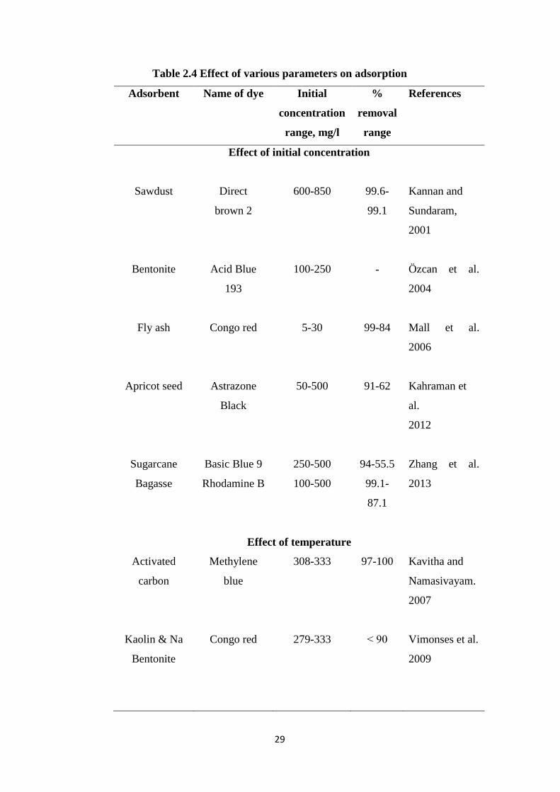
29
Table 2.4 Effect of various parameters on adsorption
Adsorbent Name of dye Initial
concentration
range, mg/l
%
removal
range
References
Effect of initial concentration
Sawdust Direct
brown 2
600-850 99.6-
99.1
Kannan and
Sundaram,
2001
Bentonite
Acid Blue
193
100-250
-
Özcan et al.
2004
Fly ash
Congo red
5-30
99-84
Mall et al.
2006
Apricot seed
Astrazone
Black
50-500
91-62
Kahraman et
al.
2012
Sugarcane
Bagasse
Basic Blue 9
Rhodamine B
250-500
100-500
94-55.5
99.1-
87.1
Zhang et al.
2013
Effect of temperature
Activated
carbon
Methylene
blue
308-333 97-100 Kavitha and
Namasivayam.
2007
Kaolin & Na
Bentonite
Congo red 279-333 ˂ 90 Vimonses et al.
2009
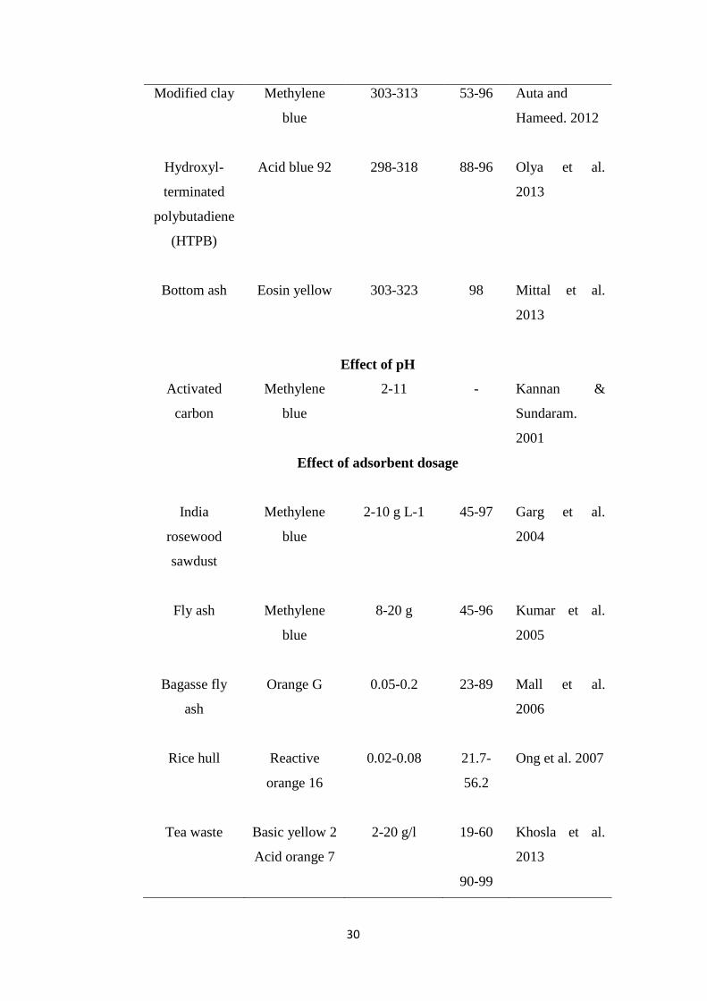
30
Modified clay Methylene
blue
303-313 53-96 Auta and
Hameed. 2012
Hydroxyl-
terminated
polybutadiene
(HTPB)
Acid blue 92 298-318 88-96 Olya et al.
2013
Bottom ash
Eosin yellow
303-323
98
Mittal et al.
2013
Effect of pH
Activated
carbon
Methylene
blue
2-11 - Kannan &
Sundaram.
2001
Effect of adsorbent dosage
India
rosewood
sawdust
Methylene
blue
2-10 g L-1 45-97 Garg et al.
2004
Fly ash Methylene
blue
8-20 g 45-96 Kumar et al.
2005
Bagasse fly
ash
Orange G 0.05-0.2 23-89 Mall et al.
2006
Rice hull Reactive
orange 16
0.02-0.08 21.7-
56.2
Ong et al. 2007
Tea waste Basic yellow 2
Acid orange 7
2-20 g/l 19-60
90-99
Khosla et al.
2013
31
2.13 Ozonation
The ozone is one of the most effective chemical oxidation process for
decolourization of wastewater having refractory organic matter which resist
biodegradation (Dogruel et al. 2006).
2.13.1 Effect of pH
Ozone decomposes into its highly reactive species like HO•, HO2• and HO3• and
occurs in an alkaline environment while at lower pH (acidic conditions) ozone
exists in its molecular state and reacts with unsaturated chromophoric bonds of
dye molecule through direct reactions (Carmen and Daniela;
www.intechopen.com).
At ozone concentration of 2970 mg/l, the simulated reactive dye bath effluent at
pH 7 showed remarkable decolourization while remained unchanged at pH 11
(Arslan et al. 2002). The decolourization of the Reactive Yellow 84 decreased
as solution pH decreased from 6.1 to 3.2 (Koch et al, 2002). The 32% reduction
in the dye decolourization time achieved as the pH of dye solution was changed
from 2 to 12 (Konsowa et al. 2003). A remarkable decrease in liquor colour
observed at pH 9 during ozonation (Beltran et al., 2006). The amount of reacted
ozone and time of ozonation are lower for Reactive dye at the pH of 3 to 5
while in case of Direct Pink, the suitable pH was found to be between 7 to 10
(Guendy, et al. 2007). The decolourization of 40.6% was achieved for pH 3.0
and 67.5% for pH 9.1 (Somensi et al. 2010). The colour of a reactive dye was
reduced to 69.69% at pH 12 with complete RO16 degradation within 8 minutes
(Turhan et al. 2013).
2.13.2 Effect of concentration on ozonation treatment
At higher initial dye concentration of textile wastewater, more ozone
consumption was observed (Lin et al., 1993, Sevimli and Sarikaya, 2002). A
complete decolourization of exhaustive reactive dye wastewater was achieved at
ozone consumption of 76.5 mg/l after ozonation for 40 minutes (Sundrarajan et
al. 2007).
32
2.13.3 Effect of ozonation on biodegradability
A study by Tarragona et al., 2015 indicated that the toxicity effects of 2,4-DCP
decreased due to ozonation. The lag phase was remarkably reduced and the
maximal SOUR increased with increase in ozone reaction time. An increase of
the biodegradable COD fraction was also observed (Aken et al 2015). The
ozonation pre-treatment enhanced the biodegradability of distillery wastewater
in an anaerobic digester treatment (Ordono et al 2012). The biodegradability
index of textile wastewater increased by 1.6 times at ozonation dosage of 300
mg/dm3
(Sevimli and Sarikaya, 2002). The less toxicity and remarkable
biodegradability improvement was found in ozonated wastewater of textile dyes
(Arslan Alaton, 2003). The simulated reactive dye and reactive yellow 84
biodegradability reached to 80 times (Koch et al., 2002).
2.13.4 Effect of ozonation time
The pulp and paper mill effluent having initial COD of 360 mg/l showed
complete decolourization after 60 minutes of ozonation time at ozone of 3g/h
(He et al. 2016). The 97% colour removal achieved with 20 mg/min of ozone
dosage (Solmaz et al , 2006). The 99% colour removal was observed in 10
minutes with 6.0, 7.5 and 9.0 dm3/min ozone dosages (Ciardelli and Ranieri.
2000). The complete colour removal is achieved within 20-60 minutes (Selçuk.
2005). The industrial sample having reactive black 5 dye completely
decolourized within 10 minutes (Colindreset al, 2010). The colour removal was
60% after 5 minutes, 80% after 10 minutes, 85% after 12.5 minutes and 90%
after 20 minutes (Meriçet al. , 2005).
2.14 Biological treatment methods
The black liquor study conducted with anaerobic baffled reactor showed the
maximum COD reduction of about 60% at an organic loading rate of 5 kg/ m3/d
at a hydraulic retention time of 2 days, pH of 8.0 and temperature of 35 °C
(Grover et al. 1999). The COD removal of 84.3% and biogas production of 21.2
l/d were observed at hydraulic retention time of 23 hours and temperature of 35
°C (Sridhar et al 2015). The UASB reactor has found to be effective for the
anaerobic digestion of pulp & paper mill wastes (Kamali et al. 2016).
33
The anaerobic digestion of black liquor of cereal straw pulping mill in batch
UASB reactor showed up to 60% COD removal efficiency at organic loading
rates of 5-10 kg COD /m3/day (Dangcong et al. 1993). The decolourization of
70-80% and COD removal of 60% was achieved with white rot fungus Trametes
versicolor treatment of black liquor of soda pulping mill (Font et al. 2003). The
lignolytic fungus Phanerochaete chrysosporium showed decolourization, COD
removal and BOD removal of 86.4%, 78.8% and 70.5%, respectively
(Jaganathan et al. 2009). The black liquor and bleach effluent from Kraft
pulping processes showed 63% COD removal with mixture of six strains of
bacteria i.e. Agrobacterium sp. ,Bacillus sp., E. Cloacae, Gordonia sp., P.
stutzeri and P. Putida (Chen et al. 2010). The COD removal ranged from 35-
98% and TSS removal ranged from 12-89% was found with black liquor
effluent, when treated with Diplodia oryzae and Phaerochaete chrysosporium
(Helmy et al, 2003).
The effluent of pulping liquors was treated with sulphate reducing bacteria
isolated from sediments from sediments from pulp and paper mills in Vietnam.
The treatment reduced 70-75% COD after 3 weeks, which could further
increased to 88% by further aerobic treatment after 48 hours (Hoa and Man.
2006). The effluent from the treatment with AlCl3 at pH-5 was further processed
with P. putida at pH 7 for 48 hours, leading to marginal further reductions in
colour, phenols, TSS, and COD. The sequential treatment of chemical
precipitation and putida resulted in better quality water than chemical
precipitation alone (Swamy et al 2016). A potential lignin-degrading fungal
strain, identified as Aspergillus flavus strain F10 reduced colour up to 31–51 %
and lignin content 39–61%in ten days of incubation when used as a free form,
while in immobilized condition it reduced more colour and lignin content within
6 day of treatment. The toxicity of paper and pulp effluent was measured in the
term of phytotoxicity. A high germination index of treated samples indicates
that the treatment reduced pollution load in effluent to low levels, which were
not toxic to plants (Barapatre and Jha, 2016). The maximum decolourization of
83% was achieved when 1% sucrose (C12H22O11) and 1% NH4Cl was added the
effluent containing immobilized cells of P. Chrysosporium (Gomathi et al
2012).
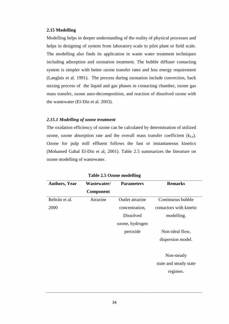
34
2.15 Modelling
Modelling helps in deeper understanding of the reality of physical processes and
helps in designing of system from laboratory scale to pilot plant or field scale.
The modelling also finds its application in waste water treatment techniques
including adsorption and ozonation treatment. The bubble diffuser contacting
system is simpler with better ozone transfer rates and less energy requirement
(Langlais et al. 1991). The process during ozonation include convection, back
mixing process of the liquid and gas phases in contacting chamber, ozone gas
mass transfer, ozone auto-decomposition, and reaction of dissolved ozone with
the wastewater (El-Din et al. 2003).
2.15.1 Modelling of ozone treatment
The oxidation efficiency of ozone can be calculated by determination of utilized
ozone, ozone absorption rate and the overall mass transfer coefficient (kLa).
Ozone for pulp mill effluent follows the fast or instantaneous kinetics
(Mohamed Gabal El-Din et al, 2001). Table 2.5 summarizes the literature on
ozone modelling of wastewater.
Table 2.5 Ozone modelling
Authors, Year Wastewater/
Component
Parameters Remarks
Beltrán et al.
2000
Atrazine
Outlet atrazine
concentration,
Dissolved
ozone, hydrogen
peroxide
Continuous bubble
contactors with kinetic
modelling.
Non-ideal flow,
dispersion model.
Non-steady
state and steady state
regimes.
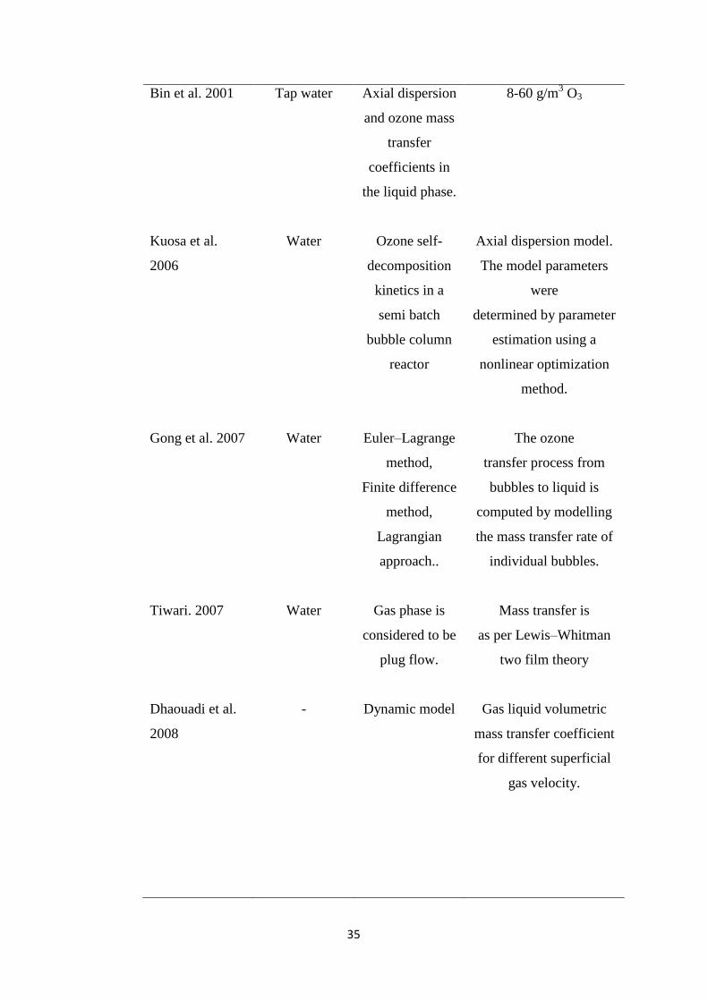
35
Bin et al. 2001 Tap water Axial dispersion
and ozone mass
transfer
coefficients in
the liquid phase.
8-60 g/m3 O3
Kuosa et al.
2006
Water Ozone self-
decomposition
kinetics in a
semi batch
bubble column
reactor
Axial dispersion model.
The model parameters
were
determined by parameter
estimation using a
nonlinear optimization
method.
Gong et al. 2007 Water Euler–Lagrange
method,
Finite difference
method,
Lagrangian
approach..
The ozone
transfer process from
bubbles to liquid is
computed by modelling
the mass transfer rate of
individual bubbles.
Tiwari. 2007 Water Gas phase is
considered to be
plug flow.
Mass transfer is
as per Lewis–Whitman
two film theory
Dhaouadi et al.
2008
- Dynamic model Gas liquid volumetric
mass transfer coefficient
for different superficial
gas velocity.
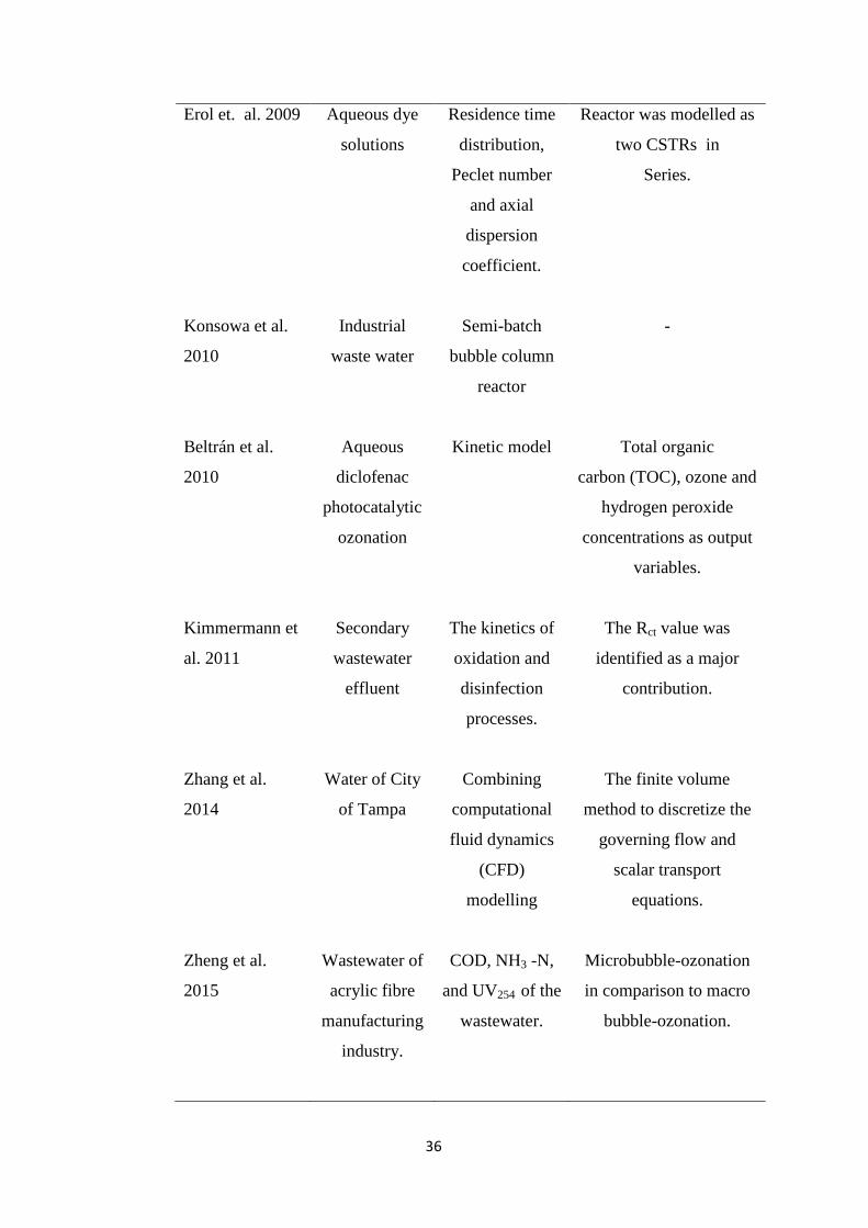
36
Erol et. al. 2009 Aqueous dye
solutions
Residence time
distribution,
Peclet number
and axial
dispersion
coefficient.
Reactor was modelled as
two CSTRs in
Series.
Konsowa et al.
2010
Industrial
waste water
Semi-batch
bubble column
reactor
-
Beltrán et al.
2010
Aqueous
diclofenac
photocatalytic
ozonation
Kinetic model Total organic
carbon (TOC), ozone and
hydrogen peroxide
concentrations as output
variables.
Kimmermann et
al. 2011
Secondary
wastewater
effluent
The kinetics of
oxidation and
disinfection
processes.
The Rct value was
identified as a major
contribution.
Zhang et al.
2014
Water of City
of Tampa
Combining
computational
fluid dynamics
(CFD)
modelling
The finite volume
method to discretize the
governing flow and
scalar transport
equations.
Zheng et al.
2015
Wastewater of
acrylic fibre
manufacturing
industry.
COD, NH3 -N,
and UV254 of the
wastewater.
Microbubble-ozonation
in comparison to macro
bubble-ozonation.
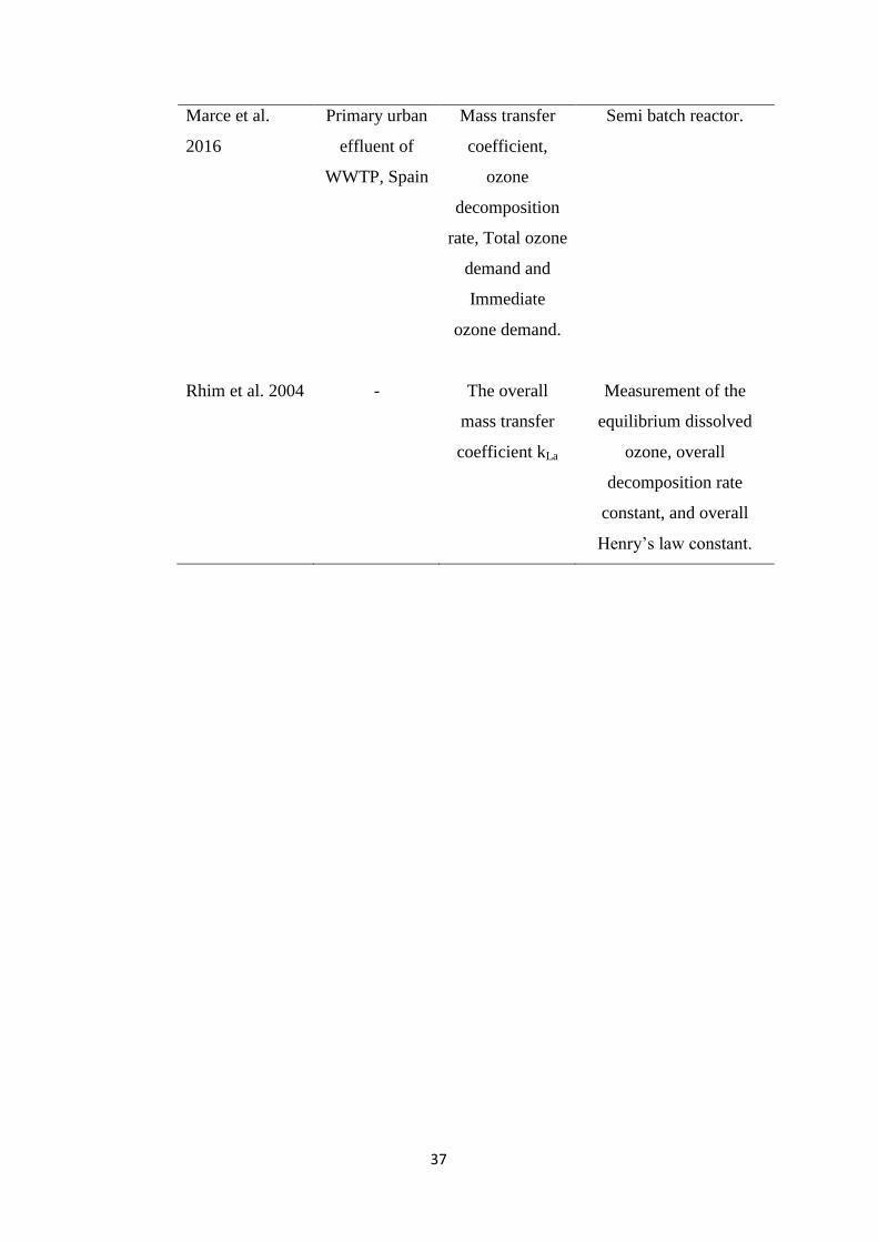
37
Marce et al.
2016
Primary urban
effluent of
WWTP, Spain
Mass transfer
coefficient,
ozone
decomposition
rate, Total ozone
demand and
Immediate
ozone demand.
Semi batch reactor.
Rhim et al. 2004 - The overall
mass transfer
coefficient kLa
Measurement of the
equilibrium dissolved
ozone, overall
decomposition rate
constant, and overall
Henry’s law constant.
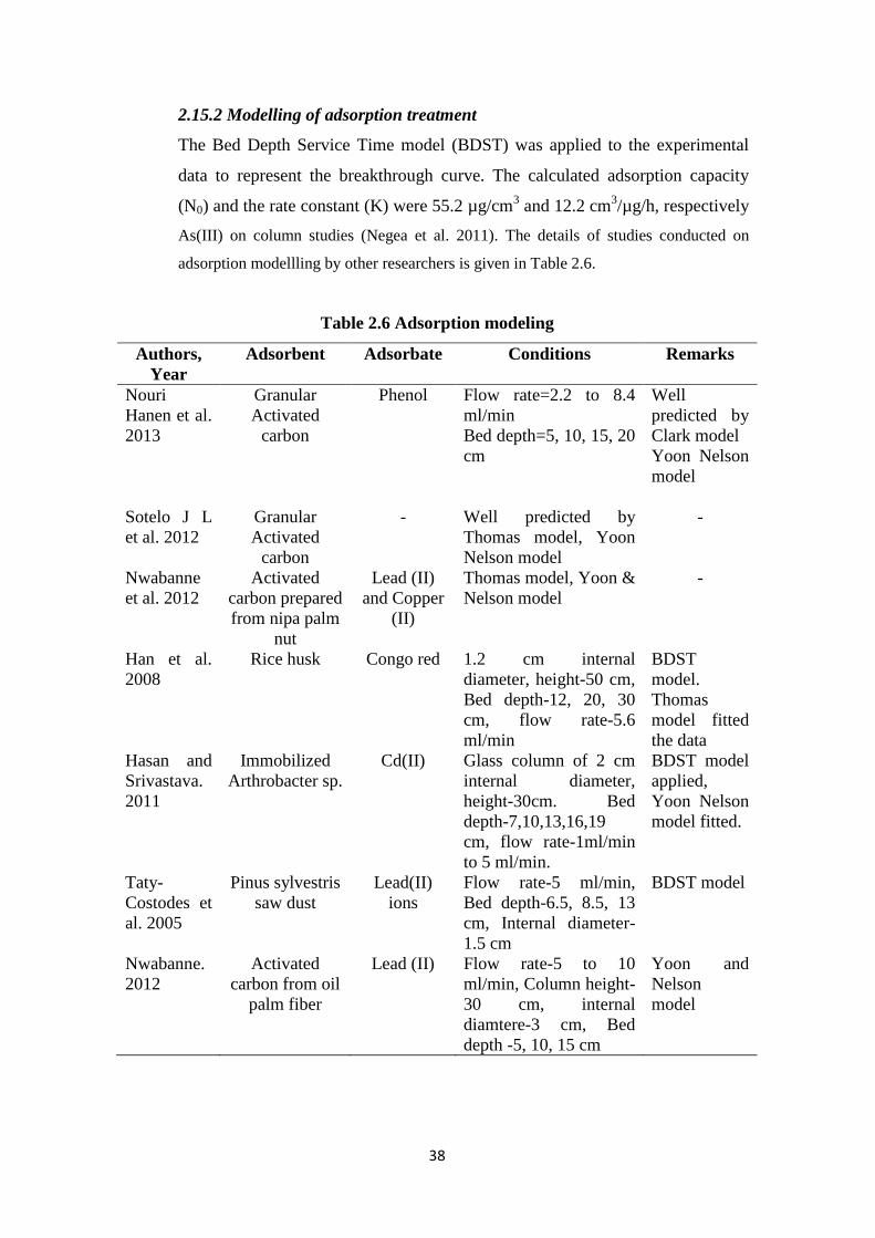
38
2.15.2 Modelling of adsorption treatment
The Bed Depth Service Time model (BDST) was applied to the experimental
data to represent the breakthrough curve. The calculated adsorption capacity
(N0) and the rate constant (K) were 55.2 µg/cm3 and 12.2 cm
3/µg/h, respectively
As(III) on column studies (Negea et al. 2011). The details of studies conducted on
adsorption modellling by other researchers is given in Table 2.6.
Table 2.6 Adsorption modeling
Authors,
Year
Adsorbent Adsorbate Conditions Remarks
Nouri
Hanen et al.
2013
Granular
Activated
carbon
Phenol Flow rate=2.2 to 8.4
ml/min
Bed depth=5, 10, 15, 20
cm
Well
predicted by
Clark model
Yoon Nelson
model
Sotelo J L
et al. 2012
Granular
Activated
carbon
- Well predicted by
Thomas model, Yoon
Nelson model
-
Nwabanne
et al. 2012
Activated
carbon prepared
from nipa palm
nut
Lead (II)
and Copper
(II)
Thomas model, Yoon &
Nelson model
-
Han et al.
2008
Rice husk Congo red 1.2 cm internal
diameter, height-50 cm,
Bed depth-12, 20, 30
cm, flow rate-5.6
ml/min
BDST
model.
Thomas
model fitted
the data
Hasan and
Srivastava.
2011
Immobilized
Arthrobacter sp.
Cd(II) Glass column of 2 cm
internal diameter,
height-30cm. Bed
depth-7,10,13,16,19
cm, flow rate-1ml/min
to 5 ml/min.
BDST model
applied,
Yoon Nelson
model fitted.
Taty-
Costodes et
al. 2005
Pinus sylvestris
saw dust
Lead(II)
ions
Flow rate-5 ml/min,
Bed depth-6.5, 8.5, 13
cm, Internal diameter-
1.5 cm
BDST model
Nwabanne.
2012
Activated
carbon from oil
palm fiber
Lead (II) Flow rate-5 to 10
ml/min, Column height-
30 cm, internal
diamtere-3 cm, Bed
depth -5, 10, 15 cm
Yoon and
Nelson
model
39
The breakthrough curve in fixed bed studies for removal of atenolol from
aqueous solutions aqueous solutions by activated carbon were predicted through
Bohart-Adams, Thomas and Yoon-Nelson models (Sotelo et al. 2012). The mass
transfer coefficient of the model was estimated. A simplified form of the dual
rate model was used to predict the column performance in terms of treatment
efficiency, consumption of carbon, and organic removal. The mass transfer
coefficients of the model were determined based on micro column experimental
data. The lower performance of the GAC column system was attributed to a
possible low efficiency in terms of carbon usage in the micro column
experiment (Zheng Zing et al 2000).
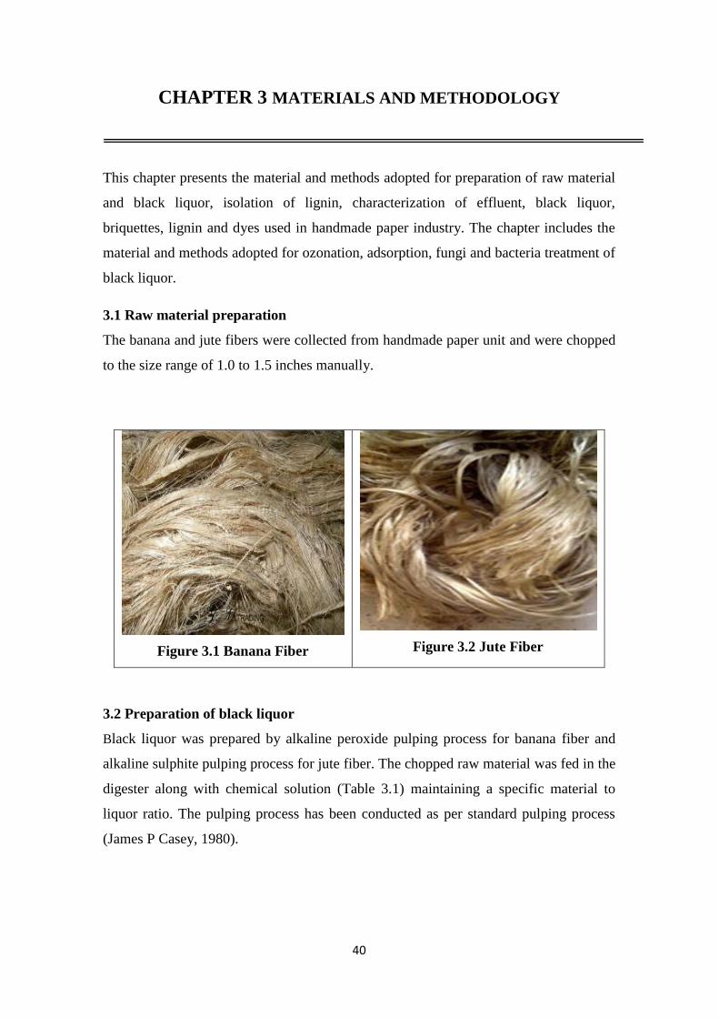
40
CHAPTER 3 MATERIALS AND METHODOLOGY
This chapter presents the material and methods adopted for preparation of raw material
and black liquor, isolation of lignin, characterization of effluent, black liquor,
briquettes, lignin and dyes used in handmade paper industry. The chapter includes the
material and methods adopted for ozonation, adsorption, fungi and bacteria treatment of
black liquor.
3.1 Raw material preparation
The banana and jute fibers were collected from handmade paper unit and were chopped
to the size range of 1.0 to 1.5 inches manually.
Figure 3.1 Banana Fiber
Figure 3.2 Jute Fiber
3.2 Preparation of black liquor
Black liquor was prepared by alkaline peroxide pulping process for banana fiber and
alkaline sulphite pulping process for jute fiber. The chopped raw material was fed in the
digester along with chemical solution (Table 3.1) maintaining a specific material to
liquor ratio. The pulping process has been conducted as per standard pulping process
(James P Casey, 1980).
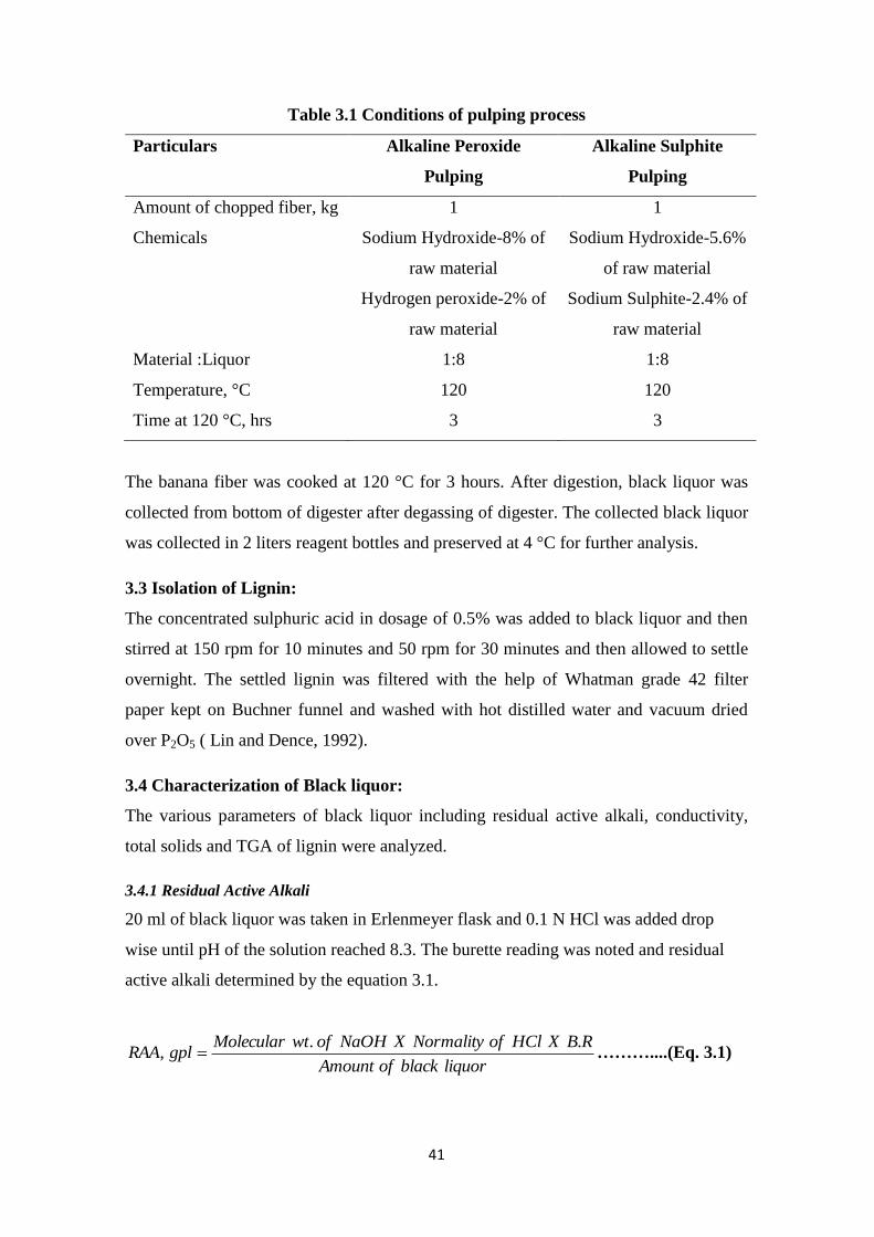
41
Table 3.1 Conditions of pulping process
Particulars Alkaline Peroxide
Pulping
Alkaline Sulphite
Pulping
Amount of chopped fiber, kg 1 1
Chemicals Sodium Hydroxide-8% of
raw material
Hydrogen peroxide-2% of
raw material
Sodium Hydroxide-5.6%
of raw material
Sodium Sulphite-2.4% of
raw material
Material :Liquor 1:8 1:8
Temperature, °C 120 120
Time at 120 °C, hrs 3 3
The banana fiber was cooked at 120 °C for 3 hours. After digestion, black liquor was
collected from bottom of digester after degassing of digester. The collected black liquor
was collected in 2 liters reagent bottles and preserved at 4 °C for further analysis.
3.3 Isolation of Lignin:
The concentrated sulphuric acid in dosage of 0.5% was added to black liquor and then
stirred at 150 rpm for 10 minutes and 50 rpm for 30 minutes and then allowed to settle
overnight. The settled lignin was filtered with the help of Whatman grade 42 filter
paper kept on Buchner funnel and washed with hot distilled water and vacuum dried
over P2O5 ( Lin and Dence, 1992).
3.4 Characterization of Black liquor:
The various parameters of black liquor including residual active alkali, conductivity,
total solids and TGA of lignin were analyzed.
3.4.1 Residual Active Alkali
20 ml of black liquor was taken in Erlenmeyer flask and 0.1 N HCl was added drop
wise until pH of the solution reached 8.3. The burette reading was noted and residual
active alkali determined by the equation 3.1.
liquorblackofAmount
RBXHClofNormalityXNaOHofwtMoleculargplRAA
.., ………....(Eq. 3.1)
42
3.4.2 Conductivity
Conductivity was determined with the help of conductivity meter (Hanna Instruments)
after calibration of conductivity meter with potassium chloride.
3.4.3 Total solids
Total solids was determined by taking black liquor & wash liquor in petri dish and kept
in oven at 105 °C for 24 hours until the weight was constant after drying. After
complete drying, total solids were determined by using the formula as given as equation
3.2.
liquorblackofWt
ovenindryingafterliquorblackofWtsolidsTotal
.
100.,%
……………(Eq. 3.2)
3.4.4 TGA Analysis of lignin
TGA is an analytical technique used to determine thermal stability of material by
monitoring the weight change that occurs as a specimen is heated. The objective of
thermal analysis is to identify temperature regimes where major weight losses (and
phase transformations) occur and decide upon the minimum sintering temperature.
TGA analysis was conducted with the help of STA 6000 (Perkin Elmeris) as per ASTM
E1131, ISO 11358.
Appropriate environment was maintained with the help of inert (usually N2) and
oxidative (O2) gas flow rates. About 15 mg of test material was placed in the specimen
holder and the temperature of the furnace was raised in steps. The initial weight reading
was set to 100%, and the heating program was initiated. The gas environment is
preselected for either a thermal decomposition (inert-nitrogen gas), an oxidative
decomposition (air or oxygen), or a thermal-oxidative combination. The sealed DSC
scans were performed at a heating rate of 5 °C/min from 30 to 400 °C under nitrogen
environment. Loss of weight at every step of temperature rise was automatically
recorded.
43
3.5 Characterization of raw water and effluent of handmade paper industry
The raw water was characterized for total hardness and chloride content.
Total Hardness It was measured using Ethylene Di amine Tetra Acetic Acid as titrant
with few drops of ammonium hydroxide buffer solution and Erichrome Black T as
indicator.
Chloride content It was determined by Mohr’s method using silver nitrate as titrant
and potassium chromate solution as indicator.
The effluent of handmade paper industry was characterized for parameters like BOD,
COD, and colour as per standard testing method of Standard Methods of Examination
of Water & Waste water (APHA, 20th
edition 1998). The sample was centrifuged at
10,000 g to remove the suspended matter. The pH of the supernatant was adjusted to 7.6
and absorbance was measured at 465 nm as per Canadian Pulp & Paper Association
(1974). The A465 values were transformed into colour units (CU) according to the
formula where A1 is the absorbance of 500 CU platinum–cobalt standard solution
(A465=0.132) and A2 is the absorbance of the wastewater sample (CPPA, 1974;
Barapatre and Jha. 2016). The colour can be determined as given in equation 3.3.
Color, 2
1500A
APCU ………………………………………………………..(Eq. 3.3)
Where,
A1=Absorbance of sample
A2=Absorbance of 500 units of Platinum Cobalt standard
3.6 Characterization of dyes used in handmade paper industry
The dyes being used in handmade paper industry was characterized for pollution
parameters like BOD, COD, and colour as per standard testing method of Standard
Methods of Examination of Water & Waste water (APHA 1998).
44
3.6.1 Determination of maxima
The black dye of 50 mg/l concentration was scanned in the range of 200–1100 nm with
the help of double beam UV-Vis. spectrophotometer (Shimadzu UV 1800), Shimadzu
for determination of wavelength corresponding to maximum absorbance.
3.7 Adsorption treatment
3.7.1 Preparation of Fly Ash
Fly ash was received from Thermal Power Plant, Yamuna Nagar. 500 g of fly ash was
washed with distilled water and dried in oven at 103 ºC for 3 hours. The dried fly ash
was passed through several sieves of ASTM No. 50, 80, 100, 170, 200, 270, 300 and
325 to get fly ash of various particle sizes and collected in polythene bags for further
study.
3.7.2 Preparation of dye solution
Commercial grade Indosol Black dye of Clariant make, Mumbai which is widely used
in handmade paper industry, was taken for the study. The direct black dye samples of
various concentrations i.e. 30, 40, 50, 100, 150 and 200 mg/l were prepared by dilution
of the stock dye solution for further studies.
3.7.3 Simulation of effluent of handmade paper industry
A stock of a mixture of commercial dyes, i.e., Direct Orange 26, Direct Navy Blue 6
and Direct Violet 66 was simulated in the laboratory in a specific ratio to simulate
actual composition of the effluent from handmade paper industry and treated as a stock
solution of 1000 mg/l. The ratio of Direct Navy Blue: Direct Orange: Direct Violet is 1:
0.2:2. The stock solution was preserved and used for further studies by dilution of stock
solution.
3.7.4 Characterization of fly ash
The characterization of fly ash included measurement of surface area, particle size
distribution and analysis of other morphological and elemental parameters using SEM,
XRD and FTIR.
45
3.7.4.1 Surface area measurement
The specific surface area of fly ash was determined using methylene blue adsorption
test (MBT) method. The surface area covered by one methylene blue molecule is
typically assumed to be 130 Å2
(1 Å = 0.1 nm) (Santamarina et al. 2002). 1 g of fly ash
was dissolved in 300 ml of methylene blue solution of different concentration i.e. 3, 6,
9, 12 and 15 mg/l. Stirring of methylene blue solution with fly ash was carried out for 2
hours and then it was kept for 24 hours to reach equilibrium. The samples were
collected and centrifuged at 13500 RPM for spectrophotometric studies. The specific
surface area was calculated from the amount of adsorbed methylene blue.
MBAMBmMB MNaqS /10 20 …………………………………………………….(Eq. 3.4)
A stock solution of 1000 mg/l was prepared by dissolving 1.127g Methylene blue, dried
at 110°c for 2 hours before use, in 1000 ml distilled water (Omomnhenle et al., 2006).
The stock solution was diluted to make solution of 3, 6, 9, 12 and 15 mg/l. The
absorbance of each concentration of methylene Blue was determined at 630nm with the
help of UV – Visible spectrophotometer (Chongrak et al. 1998).
3.7.4.2 Particle size distribution of fly ash
100 g of fly ash was fed to an ash sieve shaker in which sieves of ASTM no. 50, 80,
100, 170, 200, 270, 300, and 325 were stacked from top to bottom. The fly ash in
different screens was collected and weighed for determination of particle size
distribution.
46
3.7.4.3 Details of microstructure by SEM studies
The surface morphology of raw and adsorbed fly ash samples was characterized by
Scanning Electron Microscope (Nova Nano FE-SEM 450 FET) with accelerating
voltage of 5 kV and magnification of x500 to x5000 and field emission gun SEM at
Malaviya National Institute of Technology Jaipur. The FESEM is coupled to EDX
detector for measuring the elemental composition of nano- materials. Particles were
slightly carbon coated before analysis to make their surface more conductive. X ray
analysis was done in spot mode at 25 kV.
3.7.4.4 X- Ray Diffraction Studies
The X- Ray Diffraction studies of original fly ash and adsorbed fly ash were conducted
with the help of X-Ray Diffractometer (Panalytical X Pert Pro) with CuKα radiation at
wavelength of 1.540 A° and scans were carried out with 0.03° step and 1 second. The
identification of compounds was done by High score plus software.
3.7.4.5 Infrared Spectroscopy studies
The Fourier Transform Infrared Spectroscopy (FTIR) was carried out at room
temperature using Perkin Elmer version 10.4 Spectrophotometer in the spectral range of
4000 to 400 cm–1
with a resolution of 4 cm–1
with KBr disc method. The KBr disks of
samples were prepared by mixing 1 to 1.5 mg of sample finely grounded with
approximately 200 mg of KBr (FTIR grade) in vibratory ball mixer for 20 s. The KBr
disks were prepared under vacuum in standard device.
3.7.4.6 Addition of fly ash as filler in paper making
The adsorbed fly ash was dried at 60 °C and vacuum dried over P2O5 and further stored
in polythene bags for its utilization as filler in handmade paper making. The cotton
pulp beaten up to 400 ml freeness level, collected from the pilot plant of the Kumarappa
National Handmade Paper Institute was used to conduct the studies. The stock solution
of retention aid of 1000 mg/l was prepared to study increase in retention of fly ash on
cotton fiber after addition of retention aid to the pulp slurry. The adsorbed fly ash was
added in dosages of 2.5 & 5 % (w/w) and retention aid, 1,2-Ethanediamine, polymer
with chloromethyloxirane and N-methyl methanamine (Catiofast of BASF India
Limited) in dosage of 0.15% (w/w) on the basis of oven dry weight of cotton pulp was
added to the cotton pulp for the studies.
47
3.8 Ozonation treatment
3.8.1 Preparation of dye solution and black liquor for Ozonation treatment
Commercial grade Indosol Direct Red and Indosol Blue GLL p of Clarian make, which
is widely used in handmade paper industry, was taken for the study. Stock solutions of
1000 mg/l concentration of both direct red and direct blue dyes were prepared by
dissolving dry powdered dye in 1000 ml of distilled water. The stock solution was
diluted to prepare dye solutions of various concentrations.
3.8.2 Determination of Dissolved ozone
The dissolved ozone in collected samples were measured by indigo method by
analyzing absorbance at 600 nm with the help of double beam UV-Vis
spectrophotometer as per standard testing method no. ASTM D7677-11.
fbV
AozoneDissolved 100 ………………………………………..……...(Eq. 3.5)
Where, f = 0.42.
3.8.3 Determination of residual ozone
The measured amount of 2% KI solution is taken in gas bottle and the residual ozone is
passed into it for a specific time. The sample was drawn and 1 ml of 4N sulphuric acid
was added instantly and titrated against 0.1N sodium thiosulphate.
FactorDilutionXtakensasmpleml
NXXreadingBuretteozoneresidual
1.024 ……….(Eq. 3.6)
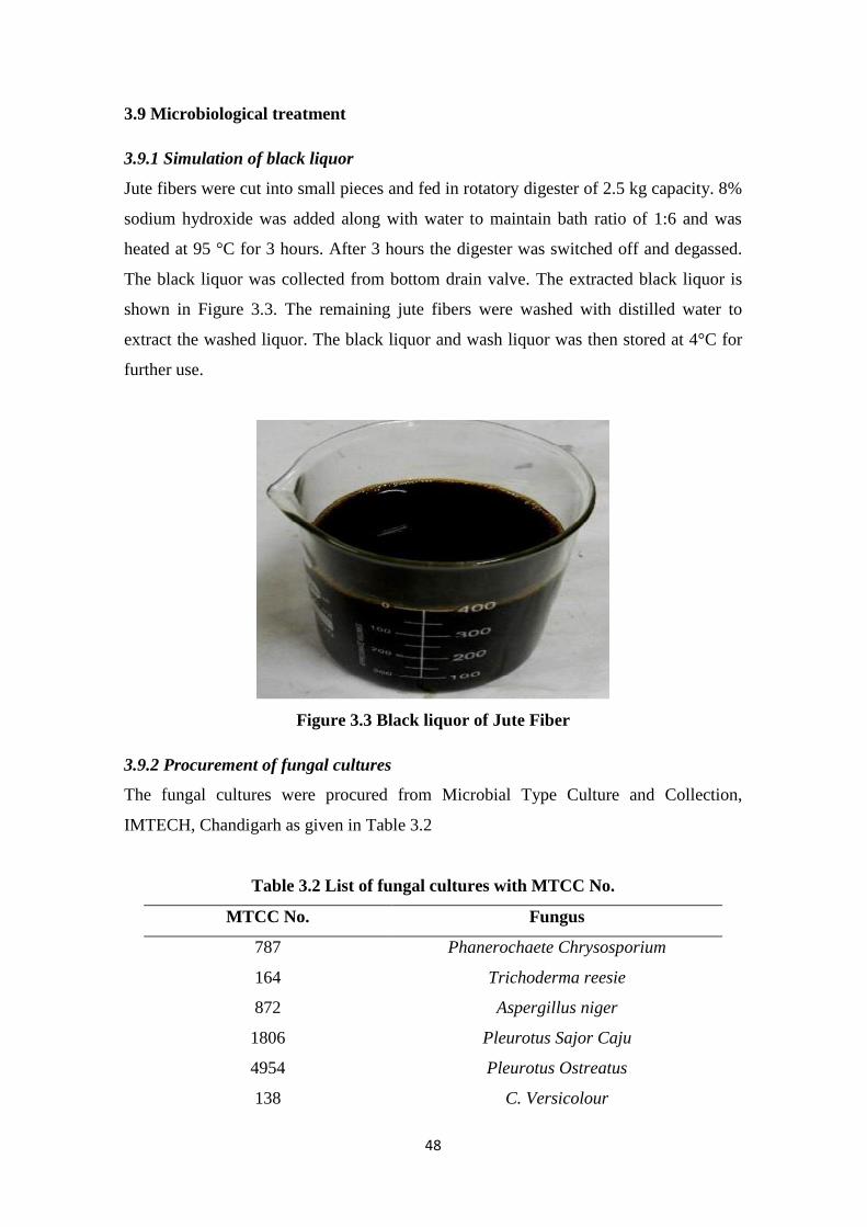
48
3.9 Microbiological treatment
3.9.1 Simulation of black liquor
Jute fibers were cut into small pieces and fed in rotatory digester of 2.5 kg capacity. 8%
sodium hydroxide was added along with water to maintain bath ratio of 1:6 and was
heated at 95 °C for 3 hours. After 3 hours the digester was switched off and degassed.
The black liquor was collected from bottom drain valve. The extracted black liquor is
shown in Figure 3.3. The remaining jute fibers were washed with distilled water to
extract the washed liquor. The black liquor and wash liquor was then stored at 4°C for
further use.
Figure 3.3 Black liquor of Jute Fiber
3.9.2 Procurement of fungal cultures
The fungal cultures were procured from Microbial Type Culture and Collection,
IMTECH, Chandigarh as given in Table 3.2
Table 3.2 List of fungal cultures with MTCC No.
MTCC No. Fungus
787 Phanerochaete Chrysosporium
164 Trichoderma reesie
872 Aspergillus niger
1806 Pleurotus Sajor Caju
4954 Pleurotus Ostreatus
138 C. Versicolour
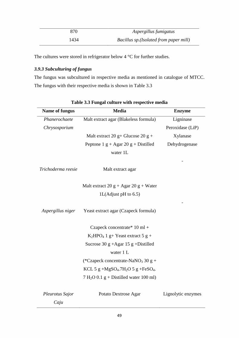
49
870 Aspergillus fumigatus
1434 Bacillus sp.(Isolated from paper mill)
The cultures were stored in refrigerator below 4 °C for further studies.
3.9.3 Subculturing of fungus
The fungus was subcultured in respective media as mentioned in catalogue of MTCC.
The fungus with their respective media is shown in Table 3.3
Table 3.3 Fungal culture with respective media
Name of fungus Media Enzyme
Phanerochaete
Chrysosporium
Malt extract agar (Blakeless formula)
Malt extract 20 g+ Glucose 20 g +
Peptone 1 g + Agar 20 g + Distilled
water 1L
Ligninase
Peroxidase (LiP)
Xylanase
Dehydrogenase
Trichoderma reesie
Malt extract agar
Malt extract 20 g + Agar 20 g + Water
1L(Adjust pH to 6.5)
-
Aspergillus niger
Yeast extract agar (Czapeck formula)
Czapeck concentrate* 10 ml +
K2HPO4 1 g+ Yeast extract 5 g +
Sucrose 30 g +Agar 15 g +Distilled
water 1 L
(*Czapeck concentrate-NaNO3 30 g +
KCL 5 g +MgSO4.7H2O 5 g +FeSO4.
7 H2O 0.1 g + Distilled water 100 ml)
-
Pleurotus Sajor
Caju
Potato Dextrose Agar
Lignolytic enzymes
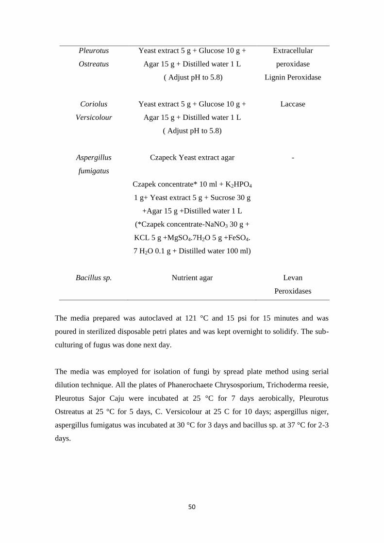
50
Pleurotus
Ostreatus
Yeast extract 5 g + Glucose 10 g +
Agar 15 g + Distilled water 1 L
( Adjust pH to 5.8)
Extracellular
peroxidase
Lignin Peroxidase
Coriolus
Versicolour
Yeast extract 5 g + Glucose 10 g +
Agar 15 g + Distilled water 1 L
( Adjust pH to 5.8)
Laccase
Aspergillus
fumigatus
Czapeck Yeast extract agar
Czapek concentrate* 10 ml + K2HPO4
1 g+ Yeast extract 5 g + Sucrose 30 g
+Agar 15 g +Distilled water 1 L
(*Czapek concentrate-NaNO3 30 g +
KCL 5 g +MgSO4.7H2O 5 g +FeSO4.
7 H2O 0.1 g + Distilled water 100 ml)
-
Bacillus sp.
Nutrient agar
Levan
Peroxidases
The media prepared was autoclaved at 121 °C and 15 psi for 15 minutes and was
poured in sterilized disposable petri plates and was kept overnight to solidify. The sub-
culturing of fugus was done next day.
The media was employed for isolation of fungi by spread plate method using serial
dilution technique. All the plates of Phanerochaete Chrysosporium, Trichoderma reesie,
Pleurotus Sajor Caju were incubated at 25 °C for 7 days aerobically, Pleurotus
Ostreatus at 25 °C for 5 days, C. Versicolour at 25 C for 10 days; aspergillus niger,
aspergillus fumigatus was incubated at 30 °C for 3 days and bacillus sp. at 37 °C for 2-3
days.
51
3.9.4 Isolation of bacteria
The bacteria were inoculated from sludge of handmade paper industry by serial dilution
method. The morphological distinct bacteria were purified by plate streak method on
agar plates containing lignin-0.2 gpl, D-glucose- 10 gpl (carbon source), peptone-5 gpl
(nitrogen source), Na2HPO4-2.4 gpl, K2HPO4-2 gpl, NH4NO3-0.1 gpl, MgSO4-0.01 gpl,
CaCl2-0.01 gpl (Chandra et al. 2007) and added in black liquor and wash liquor with 30
times dilution under aseptic conditions. The batch experiments were performed at
optimized conditions in 250 ml flasks containing 100 ml black liquor. The samples
were tested for colour and reducing sugars.
3.9.5 Treatment of effluent in batch reactor
The lignolytic fungi Phanerochaete Chrysosporium, Trichoderma reesie and
Aspergillus Niger were used to treat final effluent in batch reactor in 250 ml conical
flask. 2 g/l of glucose was added to the effluent inoculated with 5-6 g of Phanerochaete
Chrysosporium, Trichoderma reesie and Aspergillus Niger. The initial pH of the
effluent was maintained at 5.4 to 5.6 and incubated at 25 °C at 125 rpm. The samples
were withdrawn after 0, 2, 4, 5, 7, 9, 11, 14 days and analyzed for colour, reducing
sugars, pH and lignin content. The pH of the samples was adjusted to pH-5.5 with the
help of 0.1 N sulphuric acid prior to addition of fungi and to pH-8.0 prior to addition of
inoculated bacteria.
3.10 Utilization of sludge for making briquettes
The sludge of handmade paper industry was collected from handmade paper units
accumulated as waste due to fibre loss in the effluent. The collected sludge was stored
in polythene bags and kept at 4 °C for further studies. The sludge of the handmade
paper industry was mixed with black liquor with the help of domestic electric blender.
The briquettes were formed with the help of press mould after proper mixing of the
mixture and dried at room temperature for 24 hours. Then it is further dried at 60 °C for
24 hours. The briquettes were then kept in sealed polythene bags to avoid moisture.
3.10.1 Determination of calorific value
The gross calorific value of briquettes was determined as per standard testing method
no. ASTM D 5865.
52
3.11 Statistical analysis
All the samples were assayed in triplicate and the mean along with standard deviation
has been reported in the results. The mean values of these parameters obtained for
different test solutions were compared with that of control sample using students ‘t’ test
analysis at 95 % confidence level.
53
CHAPTER 4 EXPERIMENTAL SET UP
This chapter presents the experimental set up required for batch and fixed bed
adsorption studies of fly ash with direct black dye and mixture of dyes used in
handmade paper industry. The chapter includes the experimental set up of ozonation
bubble column for treatment of wastewater of handmade paper industry.
4.1 Adsorption Experimental set up
4.1.1 Batch study
Fly ash samples of size ranges (150–300 microns), (90–150 microns) and (75–90
microns) were taken for the decolourization studies. The effect of pH was studied with
black dye of 50 mg/l concentration at pH 4, 6, 8 and 10 pH was maintained with the
help of 1 N NaOH mg/l and 1N HCl. The effect of initial concentration of black dye
varying from 30 to 200 mg/l was studied at optimized pH and dosage. Batch studies
were conducted in thermostatically controlled cabinet at 200 rpm in Erlenmeyer conical
flask of 250 ml capacity. The percentage removal of dye or decolourization and amount
adsorbed was calculated by the following equation (Kumar et al., 2013).
Decolourization, % = 0
0 )(100
C
CC e ………………………………………...(Eq. 4.1)
Amount adsorbed qe (mg g-1
) = M
VCC e)( 0 ………………………………...(Eq. 4.2)
4.1.2 Column study
A borosilicate column of 1cm internal diameter and 15 cm length was taken for the
column studies. A fine mesh was introduced at the bottom of column over which a layer
of sand was spread to prevent escape of fly ash. The beds of fly ash of several bed
lengths 1.2 cm, 1.8 cm and 2.4 cm were prepared. The dye solution was fed from top to
the bed of fly ash in down flow mode. A sample of treated solution was collected at
regular intervals and analyzed with the help of double beam UV-Vis spectrophotometer.
The samples were drawn at regular interval till the concentration of effluent reached
99% of initial concentration signifying breakthrough or the exhaustion of fixed bed.
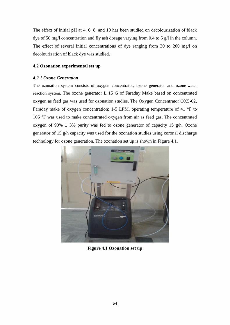
54
The effect of initial pH at 4, 6, 8, and 10 has been studied on decolourization of black
dye of 50 mg/l concentration and fly ash dosage varying from 0.4 to 5 g/l in the column.
The effect of several initial concentrations of dye ranging from 30 to 200 mg/l on
decolourization of black dye was studied.
4.2 Ozonation experimental set up
4.2.1 Ozone Generation
The ozonation system consists of oxygen concentrator, ozone generator and ozone-water
reaction system. The ozone generator L 15 G of Faraday Make based on concentrated
oxygen as feed gas was used for ozonation studies. The Oxygen Concentrator OX5-02,
Faraday make of oxygen concentration: 1-5 LPM, operating temperature of 41 °F to
105 °F was used to make concentrated oxygen from air as feed gas. The concentrated
oxygen of 90% ± 3% purity was fed to ozone generator of capacity 15 g/h. Ozone
generator of 15 g/h capacity was used for the ozonation studies using coronal discharge
technology for ozone generation. The ozonation set up is shown in Figure 4.1.
Figure 4.1 Ozonation set up
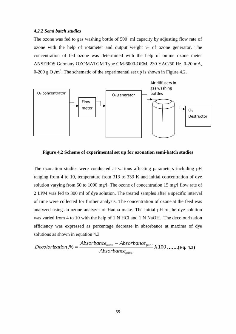
55
4.2.2 Semi batch studies
The ozone was fed to gas washing bottle of 500 ml capacity by adjusting flow rate of
ozone with the help of rotameter and output weight % of ozone generator. The
concentration of fed ozone was determined with the help of online ozone meter
ANSEROS Germany OZOMATGM Type GM-6000-OEM, 230 YAC/50 Hz, 0-20 mA,
0-200 g O3/m3. The schematic of the experimental set up is shown in Figure 4.2.
Figure 4.2 Scheme of experimental set up for ozonation semi-batch studies
The ozonation studies were conducted at various affecting parameters including pH
ranging from 4 to 10, temperature from 313 to 333 K and initial concentration of dye
solution varying from 50 to 1000 mg/l. The ozone of concentration 15 mg/l flow rate of
2 LPM was fed to 300 ml of dye solution. The treated samples after a specific interval
of time were collected for further analysis. The concentration of ozone at the feed was
analyzed using an ozone analyzer of Hanna make. The initial pH of the dye solution
was varied from 4 to 10 with the help of 1 N HCl and 1 N NaOH. The decolourization
efficiency was expressed as percentage decrease in absorbance at maxima of dye
solutions as shown in equation 4.3.
100,% XAbsorbance
AbsorbanceAbsorbancetionDecoloriza
initial
finalinitial …….(Eq. 4.3)
O3 generator O2 concentrator
Flow
meter O3
Destructor
Air diffusers in gas washing bottles
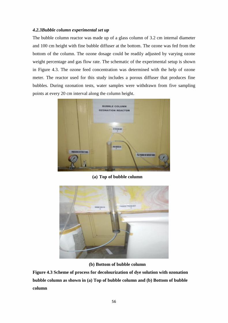
56
4.2.3Bubble column experimental set up
The bubble column reactor was made up of a glass column of 3.2 cm internal diameter
and 100 cm height with fine bubble diffuser at the bottom. The ozone was fed from the
bottom of the column. The ozone dosage could be readily adjusted by varying ozone
weight percentage and gas flow rate. The schematic of the experimental setup is shown
in Figure 4.3. The ozone feed concentration was determined with the help of ozone
meter. The reactor used for this study includes a porous diffuser that produces fine
bubbles. During ozonation tests, water samples were withdrawn from five sampling
points at every 20 cm interval along the column height.
(a) Top of bubble column
(b) Bottom of bubble column
Figure 4.3 Scheme of process for decolourization of dye solution with ozonation
bubble column as shown in (a) Top of bubble column and (b) Bottom of bubble
column
57
CHAPTER 5 –CHARACTERIZATION
The characterization studies include characterization of raw water, wastewater,
quantification of water consumption and waste water generation. The black liquor of
various raw materials at various pulping processes has been analyzed.
5.1 Characterization of raw water used in handmade paper units
The technical visits have been made to 30 handmade paper units of Sanganer region and
the raw water being used was tested for pH, Hardness and Chloride content which are
given as Table 5.1.
Table-5.1 Characterization of raw water used in handmade paper units
pH Hardness, mg/l Chloride, mg/l
Range 7.52-7.60 382-646 175-290
Mean 7.57 495 220
The higher hardness in some of the handmade paper units may be due to the presence of
many textile units in the vicinity, which are in the process of bleaching and printing the
textiles. Handmade paper unit in village Chaksu, which is 20 km from the Institute, has
shown quite low hardness of 220 mg/l as there in no textile mills near this handmade
paper industry. It has been found that the quality of raw water depends on the presence
of units, creating pollution in the surrounding area and depth of boring. As per IS No.
2724-1964 (64 Reaffirmed 1983) tolerance of various parameters have been
standardized. The tolerance limit of hardness of raw water used for making high-grade
paper is 100 mg/l while it is 200 mg/l for ground wood paper and kraft paper
unbleached and pulp unbleached.
5.2 Quantification of water consumption and waste water generation
The study of 30 handmade paper units of Sanganer showed the following results of
water consumption and waste water discharge as given in Table-5.2.
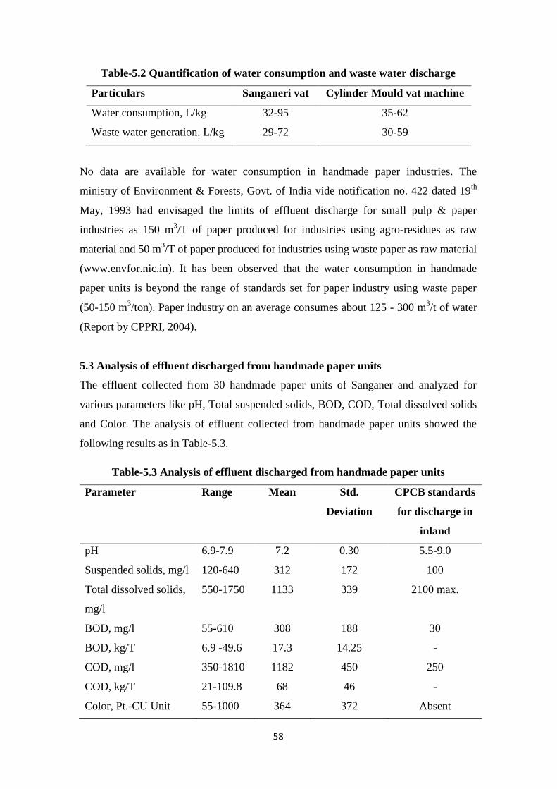
58
Table-5.2 Quantification of water consumption and waste water discharge
Particulars Sanganeri vat Cylinder Mould vat machine
Water consumption, L/kg 32-95 35-62
Waste water generation, L/kg 29-72 30-59
No data are available for water consumption in handmade paper industries. The
ministry of Environment & Forests, Govt. of India vide notification no. 422 dated 19th
May, 1993 had envisaged the limits of effluent discharge for small pulp & paper
industries as 150 m3/T of paper produced for industries using agro-residues as raw
material and 50 m3/T of paper produced for industries using waste paper as raw material
(www.envfor.nic.in). It has been observed that the water consumption in handmade
paper units is beyond the range of standards set for paper industry using waste paper
(50-150 m3/ton). Paper industry on an average consumes about 125 - 300 m
3/t of water
(Report by CPPRI, 2004).
5.3 Analysis of effluent discharged from handmade paper units
The effluent collected from 30 handmade paper units of Sanganer and analyzed for
various parameters like pH, Total suspended solids, BOD, COD, Total dissolved solids
and Color. The analysis of effluent collected from handmade paper units showed the
following results as in Table-5.3.
Table-5.3 Analysis of effluent discharged from handmade paper units
Parameter Range Mean Std.
Deviation
CPCB standards
for discharge in
inland
pH 6.9-7.9 7.2 0.30 5.5-9.0
Suspended solids, mg/l 120-640 312 172 100
Total dissolved solids,
mg/l
550-1750 1133 339 2100 max.
BOD, mg/l 55-610 308 188 30
BOD, kg/T 6.9 -49.6 17.3 14.25 -
COD, mg/l 350-1810 1182 450 250
COD, kg/T 21-109.8 68 46 -
Color, Pt.-CU Unit 55-1000 364 372 Absent
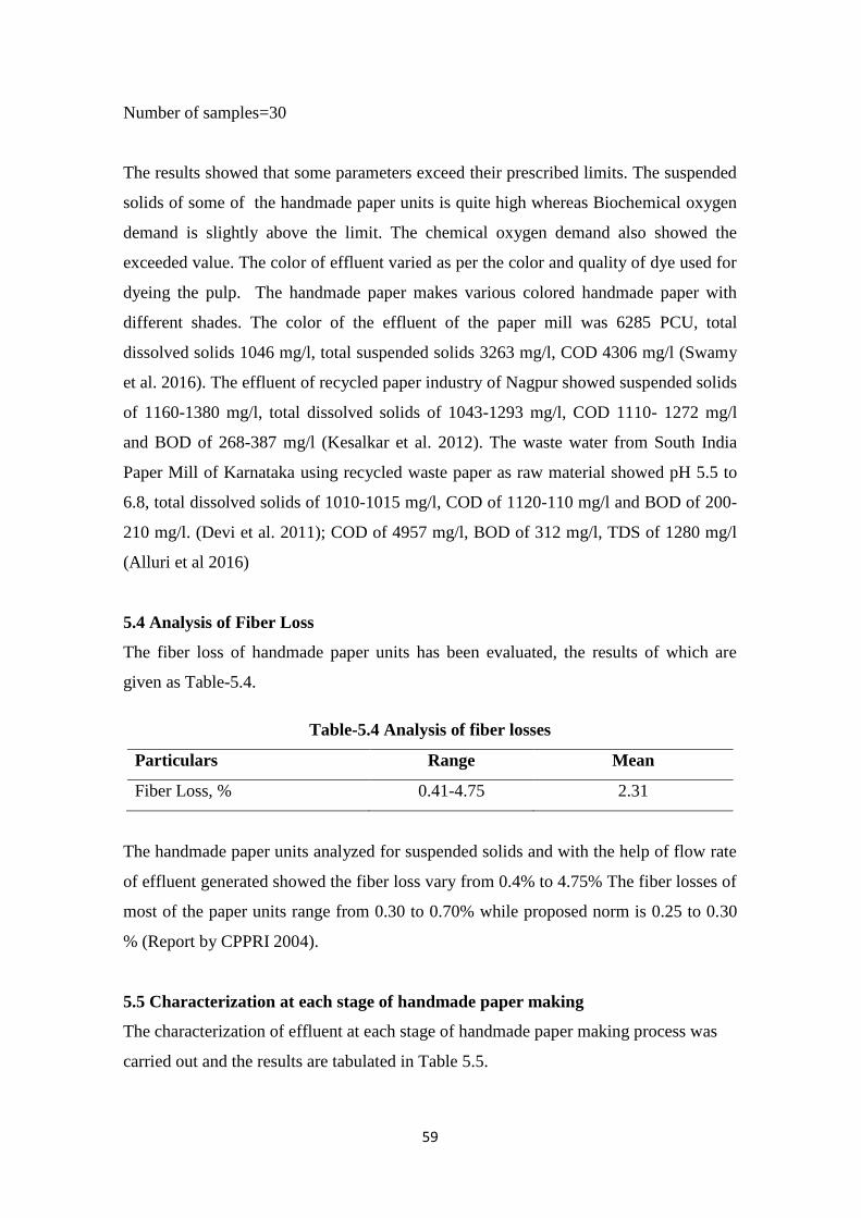
59
Number of samples=30
The results showed that some parameters exceed their prescribed limits. The suspended
solids of some of the handmade paper units is quite high whereas Biochemical oxygen
demand is slightly above the limit. The chemical oxygen demand also showed the
exceeded value. The color of effluent varied as per the color and quality of dye used for
dyeing the pulp. The handmade paper makes various colored handmade paper with
different shades. The color of the effluent of the paper mill was 6285 PCU, total
dissolved solids 1046 mg/l, total suspended solids 3263 mg/l, COD 4306 mg/l (Swamy
et al. 2016). The effluent of recycled paper industry of Nagpur showed suspended solids
of 1160-1380 mg/l, total dissolved solids of 1043-1293 mg/l, COD 1110- 1272 mg/l
and BOD of 268-387 mg/l (Kesalkar et al. 2012). The waste water from South India
Paper Mill of Karnataka using recycled waste paper as raw material showed pH 5.5 to
6.8, total dissolved solids of 1010-1015 mg/l, COD of 1120-110 mg/l and BOD of 200-
210 mg/l. (Devi et al. 2011); COD of 4957 mg/l, BOD of 312 mg/l, TDS of 1280 mg/l
(Alluri et al 2016)
5.4 Analysis of Fiber Loss
The fiber loss of handmade paper units has been evaluated, the results of which are
given as Table-5.4.
Table-5.4 Analysis of fiber losses
Particulars Range Mean
Fiber Loss, % 0.41-4.75 2.31
The handmade paper units analyzed for suspended solids and with the help of flow rate
of effluent generated showed the fiber loss vary from 0.4% to 4.75% The fiber losses of
most of the paper units range from 0.30 to 0.70% while proposed norm is 0.25 to 0.30
% (Report by CPPRI 2004).
5.5 Characterization at each stage of handmade paper making
The characterization of effluent at each stage of handmade paper making process was
carried out and the results are tabulated in Table 5.5.
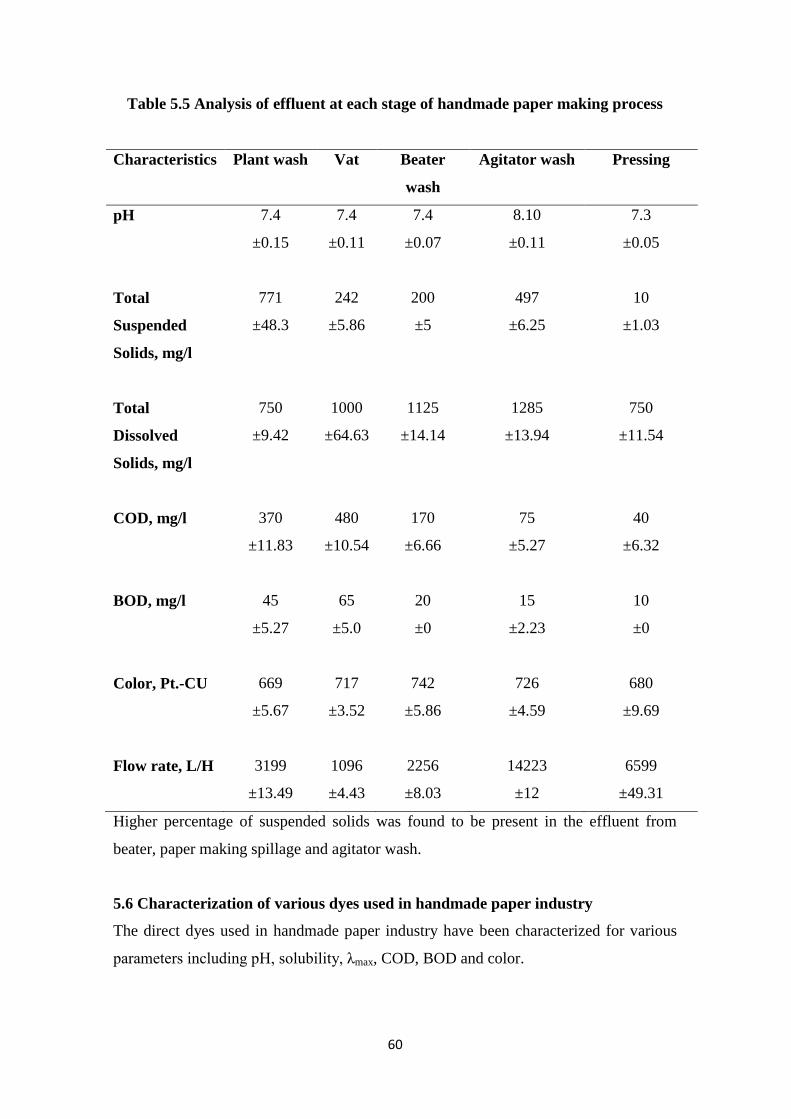
60
Table 5.5 Analysis of effluent at each stage of handmade paper making process
Characteristics Plant wash Vat Beater
wash
Agitator wash Pressing
pH 7.4
±0.15
7.4
±0.11
7.4
±0.07
8.10
±0.11
7.3
±0.05
Total
Suspended
Solids, mg/l
771
±48.3
242
±5.86
200
±5
497
±6.25
10
±1.03
Total
Dissolved
Solids, mg/l
750
±9.42
1000
±64.63
1125
±14.14
1285
±13.94
750
±11.54
COD, mg/l
370
±11.83
480
±10.54
170
±6.66
75
±5.27
40
±6.32
BOD, mg/l
45
±5.27
65
±5.0
20
±0
15
±2.23
10
±0
Color, Pt.-CU
669
±5.67
717
±3.52
742
±5.86
726
±4.59
680
±9.69
Flow rate, L/H 3199
±13.49
1096
±4.43
2256
±8.03
14223
±12
6599
±49.31
Higher percentage of suspended solids was found to be present in the effluent from
beater, paper making spillage and agitator wash.
5.6 Characterization of various dyes used in handmade paper industry
The direct dyes used in handmade paper industry have been characterized for various
parameters including pH, solubility, λmax, COD, BOD and color.
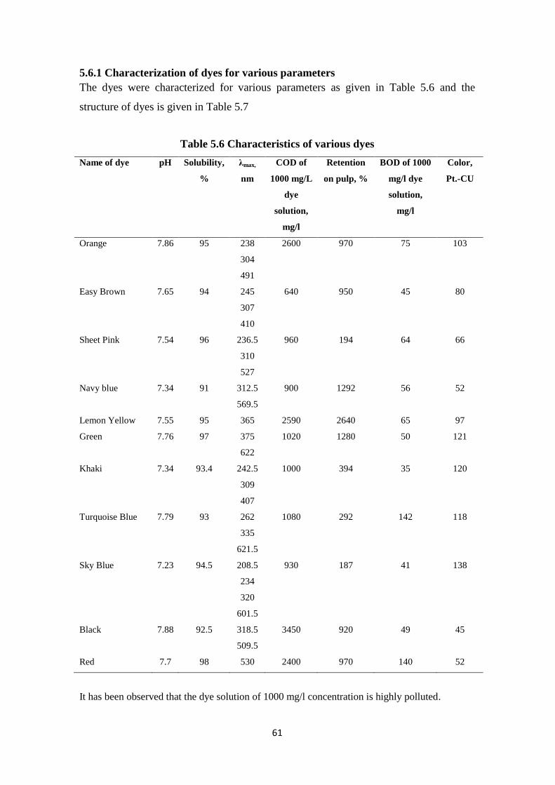
61
5.6.1 Characterization of dyes for various parameters
The dyes were characterized for various parameters as given in Table 5.6 and the
structure of dyes is given in Table 5.7
Table 5.6 Characteristics of various dyes
Name of dye pH Solubility,
%
λmax,
nm
COD of
1000 mg/L
dye
solution,
mg/l
Retention
on pulp, %
BOD of 1000
mg/l dye
solution,
mg/l
Color,
Pt.-CU
Orange 7.86 95 238
304
491
2600 970 75 103
Easy Brown 7.65 94 245
307
410
640 950 45 80
Sheet Pink 7.54 96 236.5
310
527
960 194 64 66
Navy blue 7.34 91 312.5
569.5
900 1292 56 52
Lemon Yellow 7.55 95 365 2590 2640 65 97
Green 7.76 97 375
622
1020 1280 50 121
Khaki 7.34 93.4 242.5
309
407
1000 394 35 120
Turquoise Blue 7.79 93 262
335
621.5
1080 292 142 118
Sky Blue 7.23 94.5 208.5
234
320
601.5
930 187 41 138
Black 7.88 92.5 318.5
509.5
3450 920 49 45
Red 7.7 98 530 2400 970 140 52
It has been observed that the dye solution of 1000 mg/l concentration is highly polluted.
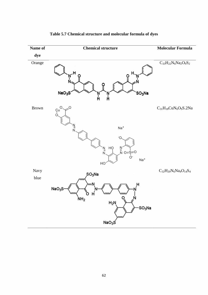
62
Table 5.7 Chemical structure and molecular formula of dyes
Name of
dye
Chemical structure Molecular Formula
Orange
C33H22N6Na2O9S2
Brown
C31H18CuN6O9S.2Na
Navy
blue
C32H20N6Na4O14S4
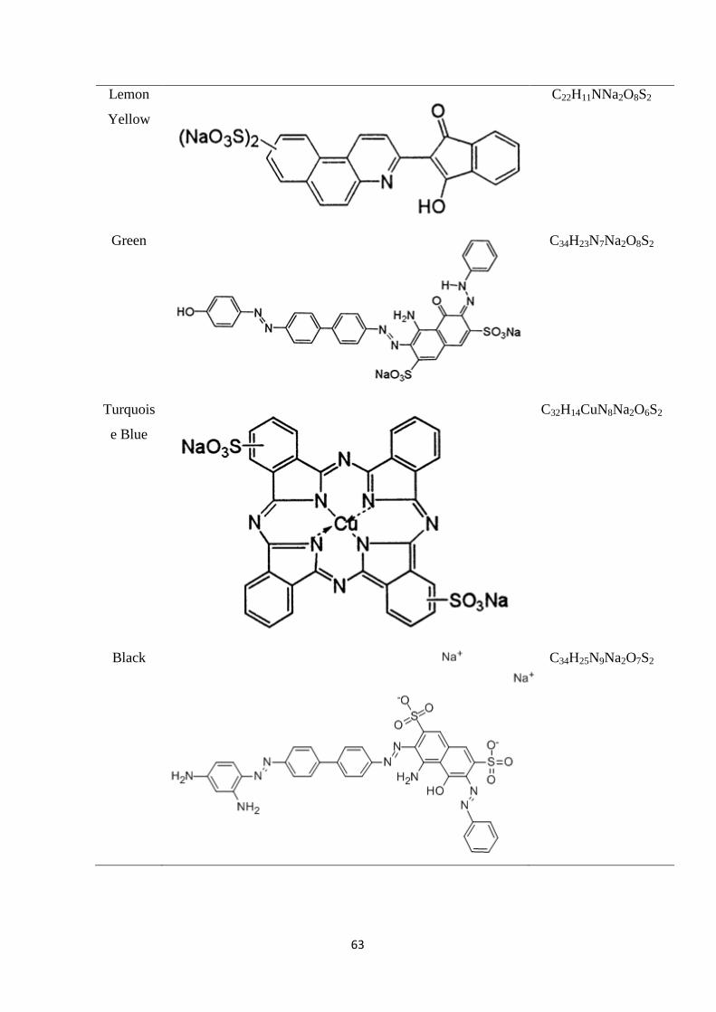
63
Lemon
Yellow
C22H11NNa2O8S2
Green
C34H23N7Na2O8S2
Turquois
e Blue
C32H14CuN8Na2O6S2
Black
C34H25N9Na2O7S2
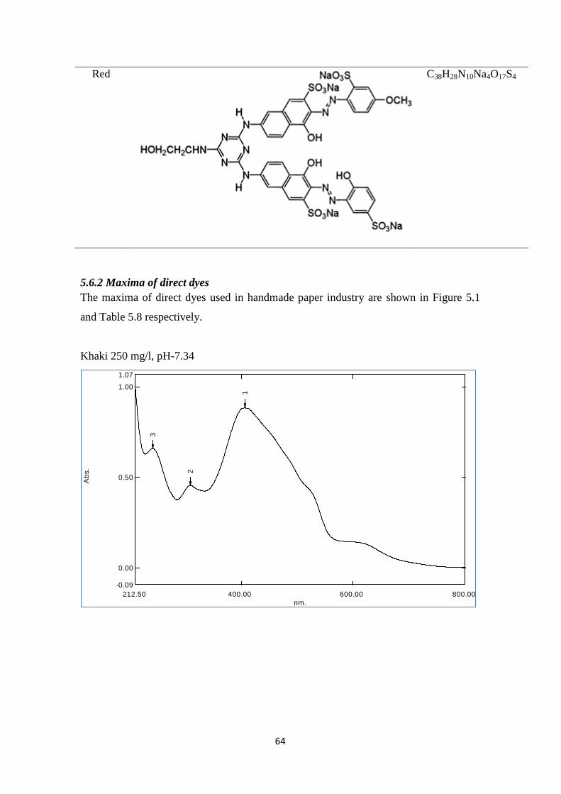
64
Red
C38H28N10Na4O17S4
5.6.2 Maxima of direct dyes
The maxima of direct dyes used in handmade paper industry are shown in Figure 5.1
and Table 5.8 respectively.
Khaki 250 mg/l, pH-7.34
nm.
212.50 400.00 600.00 800.00
Ab
s.
1.07
1.00
0.50
0.00
-0.09
1
2
3
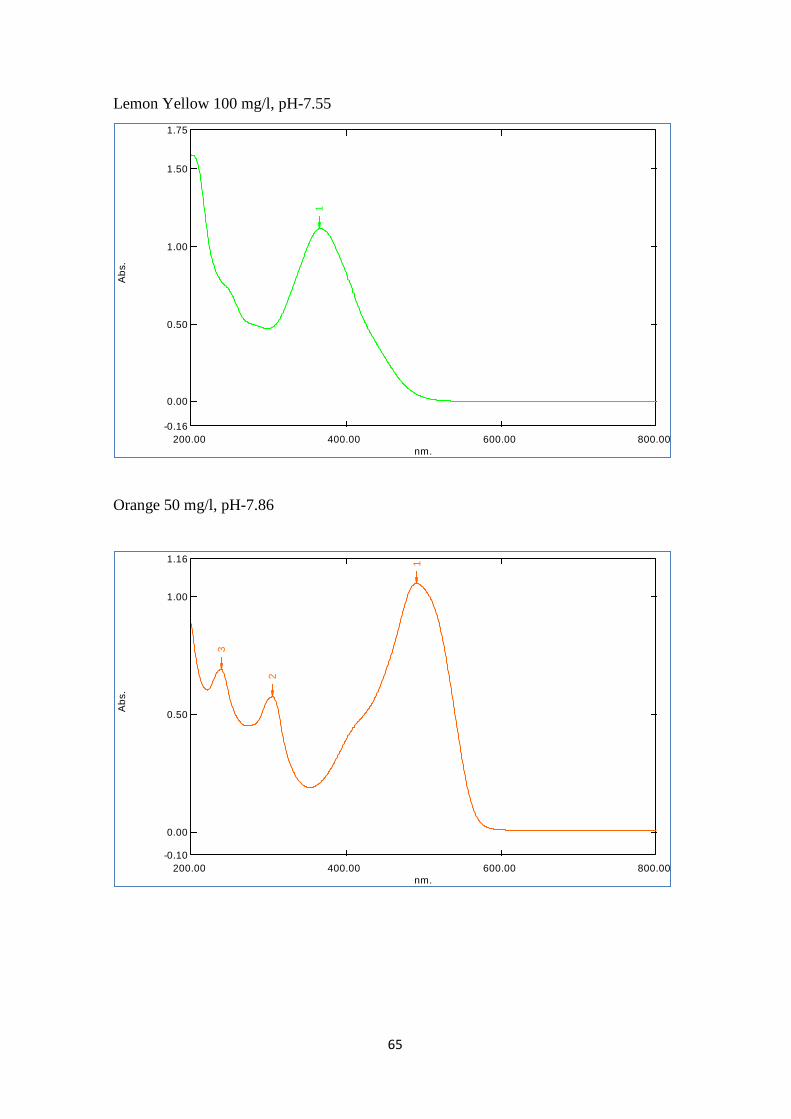
65
Lemon Yellow 100 mg/l, pH-7.55
Orange 50 mg/l, pH-7.86
nm.
200.00 400.00 600.00 800.00
Ab
s.
1.75
1.50
1.00
0.50
0.00
-0.16
1
nm.
200.00 400.00 600.00 800.00
Ab
s.
1.16
1.00
0.50
0.00
-0.10
1
2
3
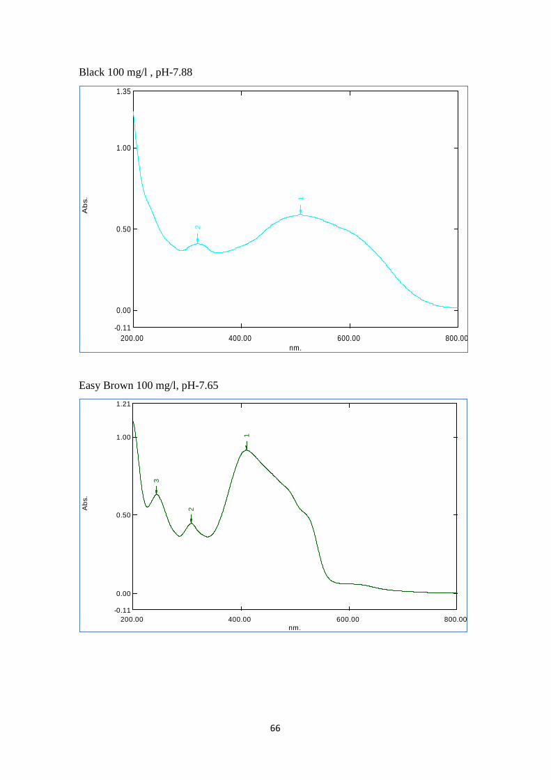
66
Black 100 mg/l , pH-7.88
Easy Brown 100 mg/l, pH-7.65
nm.
200.00 400.00 600.00 800.00
Ab
s.
1.35
1.00
0.50
0.00
-0.11
1
2
nm.
200.00 400.00 600.00 800.00
Ab
s.
1.21
1.00
0.50
0.00
-0.11
1
2
3
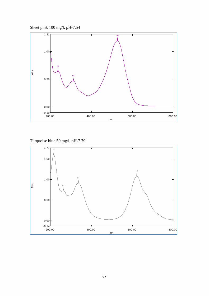
67
Sheet pink 100 mg/l, pH-7.54
Turquoise blue 50 mg/l, pH-7.79
nm.
200.00 400.00 600.00 800.00
Ab
s.
1.31
1.00
0.50
0.00
-0.10
1
2
3
nm.
200.00 400.00 600.00 800.00
Ab
s.
1.77
1.50
1.00
0.50
0.00
-0.14
1
2
3
4
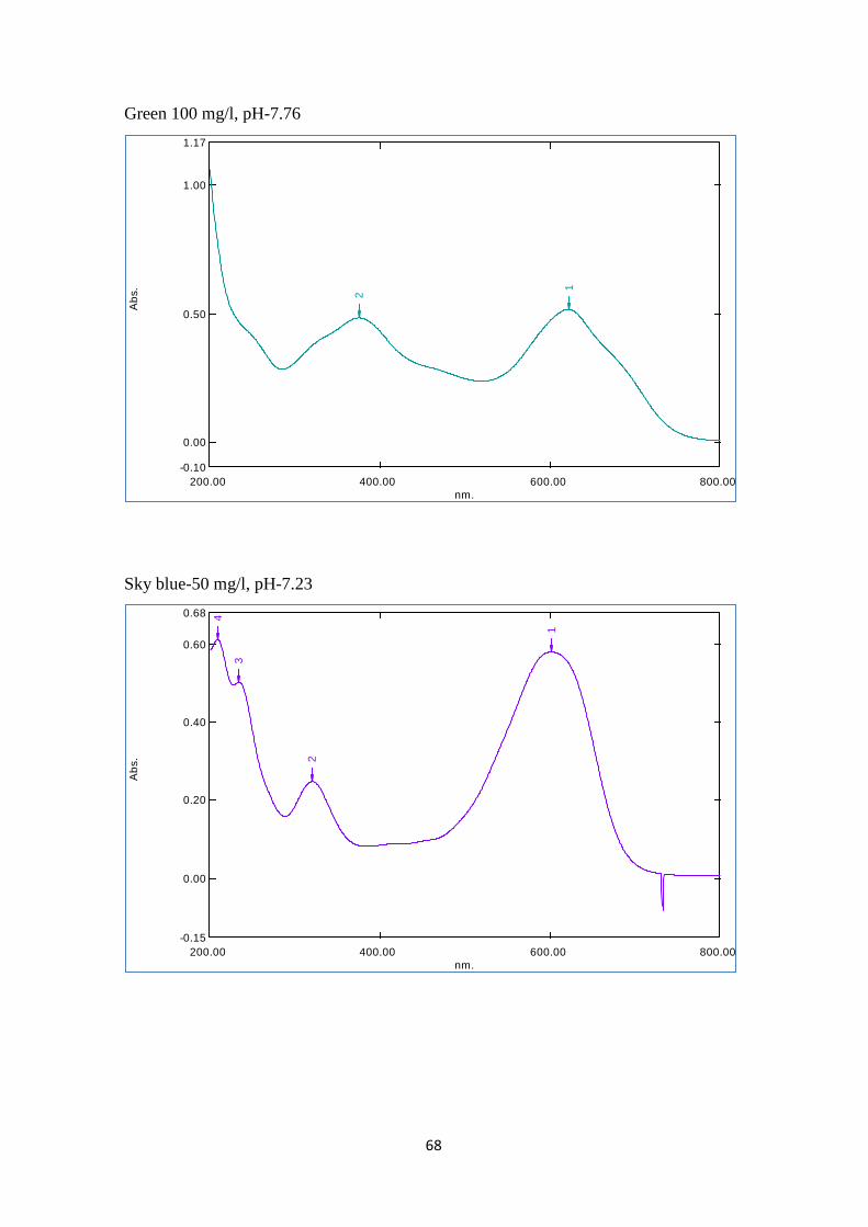
68
Green 100 mg/l, pH-7.76
Sky blue-50 mg/l, pH-7.23
nm.
200.00 400.00 600.00 800.00
Ab
s.
1.17
1.00
0.50
0.00
-0.10
1
2
nm.
200.00 400.00 600.00 800.00
Ab
s.
0.68
0.60
0.40
0.20
0.00
-0.15
1
2
3
4
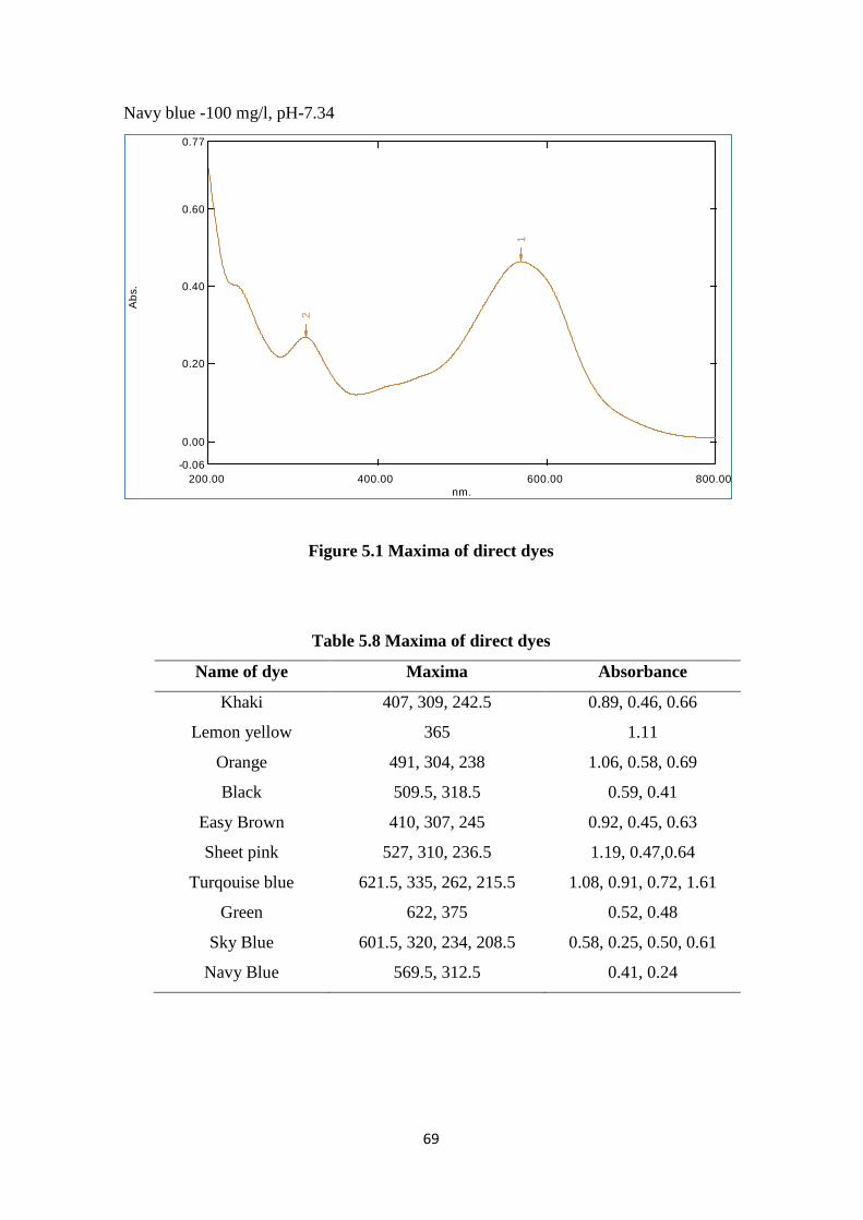
69
Navy blue -100 mg/l, pH-7.34
Figure 5.1 Maxima of direct dyes
Table 5.8 Maxima of direct dyes
Name of dye Maxima Absorbance
Khaki 407, 309, 242.5 0.89, 0.46, 0.66
Lemon yellow 365 1.11
Orange 491, 304, 238 1.06, 0.58, 0.69
Black 509.5, 318.5 0.59, 0.41
Easy Brown 410, 307, 245 0.92, 0.45, 0.63
Sheet pink 527, 310, 236.5 1.19, 0.47,0.64
Turqouise blue 621.5, 335, 262, 215.5 1.08, 0.91, 0.72, 1.61
Green 622, 375 0.52, 0.48
Sky Blue 601.5, 320, 234, 208.5 0.58, 0.25, 0.50, 0.61
Navy Blue 569.5, 312.5 0.41, 0.24
nm.
200.00 400.00 600.00 800.00
Ab
s.
0.77
0.60
0.40
0.20
0.00
-0.06
1
2
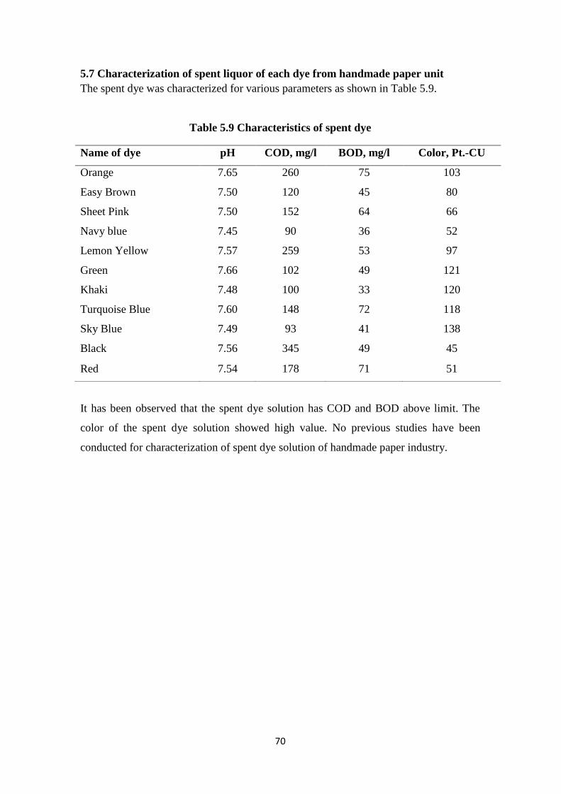
70
5.7 Characterization of spent liquor of each dye from handmade paper unit
The spent dye was characterized for various parameters as shown in Table 5.9.
Table 5.9 Characteristics of spent dye
It has been observed that the spent dye solution has COD and BOD above limit. The
color of the spent dye solution showed high value. No previous studies have been
conducted for characterization of spent dye solution of handmade paper industry.
Name of dye pH COD, mg/l BOD, mg/l Color, Pt.-CU
Orange 7.65 260 75 103
Easy Brown 7.50 120 45 80
Sheet Pink 7.50 152 64 66
Navy blue 7.45 90 36 52
Lemon Yellow 7.57 259 53 97
Green 7.66 102 49 121
Khaki 7.48 100 33 120
Turquoise Blue 7.60 148 72 118
Sky Blue 7.49 93 41 138
Black 7.56 345 49 45
Red 7.54 178 71 51
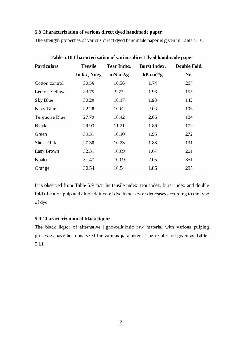
71
5.8 Characterization of various direct dyed handmade paper
The strength properties of various direct dyed handmade paper is given in Table 5.10.
Table 5.10 Characterization of various direct dyed handmade paper
Particulars Tensile
Index, Nm/g
Tear Index,
mN.m2/g
Burst Index,
kPa.m2/g
Double Fold,
No.
Cotton control 30.56 10.36 1.74 267
Lemon Yellow 33.75 9.77 1.96 155
Sky Blue 30.20 10.17 1.93 142
Navy Blue 32.28 10.62 2.03 196
Turquoise Blue 27.79 10.42 2.06 184
Black 29.93 11.21 1.86 179
Green 39.31 10.10 1.95 272
Sheet Pink 27.38 10.23 1.88 131
Easy Brown 32.31 10.69 1.67 261
Khaki 31.47 10.09 2.05 351
Orange 30.54 10.54 1.86 295
It is observed from Table 5.9 that the tensile index, tear index, burst index and double
fold of cotton pulp and after addition of dye increases or decreases according to the type
of dye.
5.9 Characterization of black liquor
The black liquor of alternative ligno-cellulosic raw material with various pulping
processes have been analyzed for various parameters. The results are given as Table-
5.11.
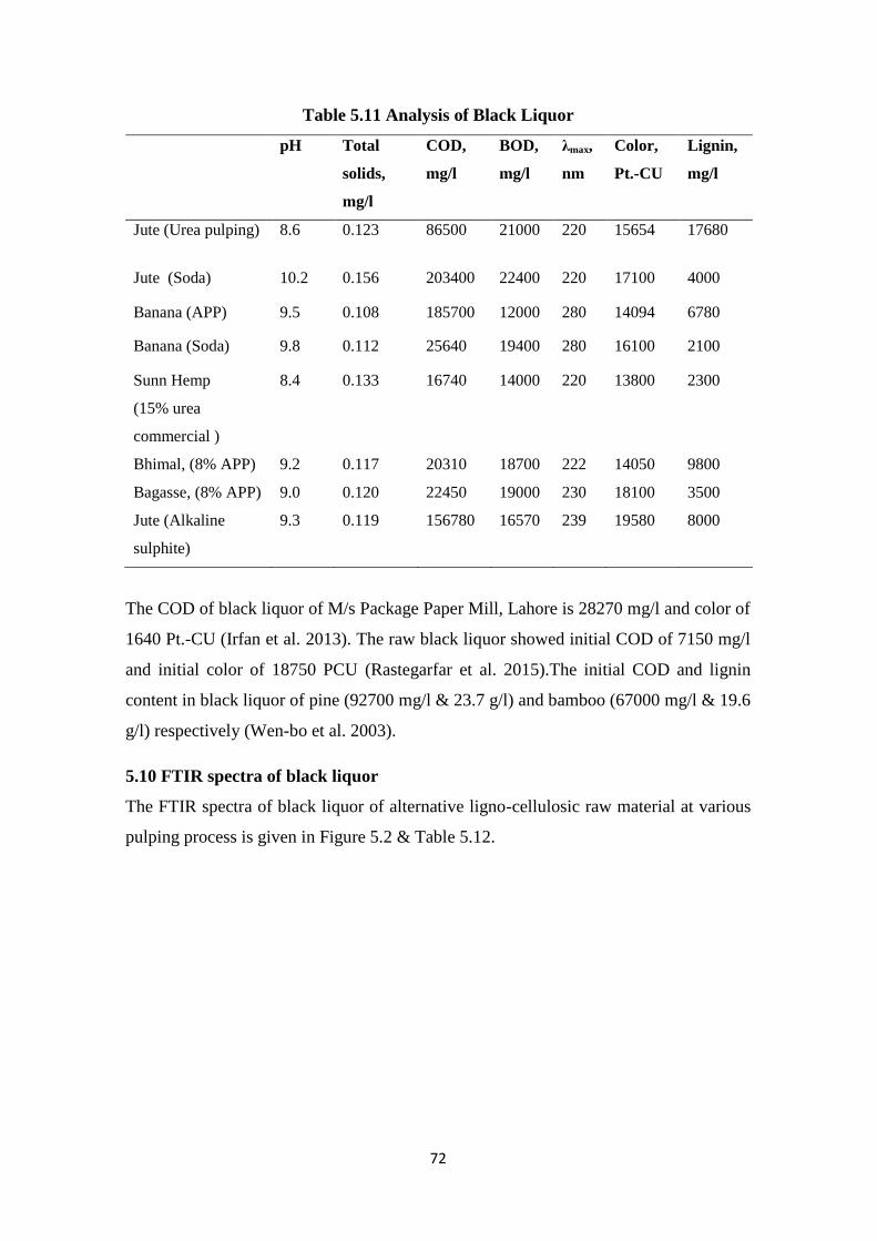
72
Table 5.11 Analysis of Black Liquor
pH Total
solids,
mg/l
COD,
mg/l
BOD,
mg/l
λmax,
nm
Color,
Pt.-CU
Lignin,
mg/l
Jute (Urea pulping) 8.6 0.123 86500 21000 220 15654 17680
Jute (Soda) 10.2 0.156 203400 22400 220 17100 4000
Banana (APP) 9.5 0.108 185700 12000 280 14094 6780
Banana (Soda) 9.8 0.112 25640 19400 280 16100 2100
Sunn Hemp
(15% urea
commercial )
8.4 0.133 16740 14000 220 13800 2300
Bhimal, (8% APP) 9.2 0.117 20310 18700 222 14050 9800
Bagasse, (8% APP) 9.0 0.120 22450 19000 230 18100 3500
Jute (Alkaline
sulphite)
9.3 0.119 156780 16570 239 19580 8000
The COD of black liquor of M/s Package Paper Mill, Lahore is 28270 mg/l and color of
1640 Pt.-CU (Irfan et al. 2013). The raw black liquor showed initial COD of 7150 mg/l
and initial color of 18750 PCU (Rastegarfar et al. 2015).The initial COD and lignin
content in black liquor of pine (92700 mg/l & 23.7 g/l) and bamboo (67000 mg/l & 19.6
g/l) respectively (Wen-bo et al. 2003).
5.10 FTIR spectra of black liquor
The FTIR spectra of black liquor of alternative ligno-cellulosic raw material at various
pulping process is given in Figure 5.2 & Table 5.12.
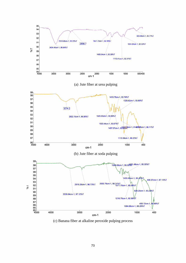
73
(a) Jute fiber at urea pulping
(b) Jute fiber at soda pulping
(c) Banana fiber at alkaline peroxide pulping process
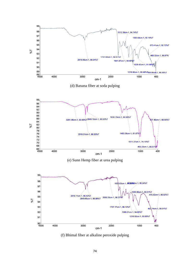
74
(d) Banana fiber at soda pulping
(e) Sunn Hemp fiber at urea pulping
(f) Bhimal fiber at alkaline peroxide pulping
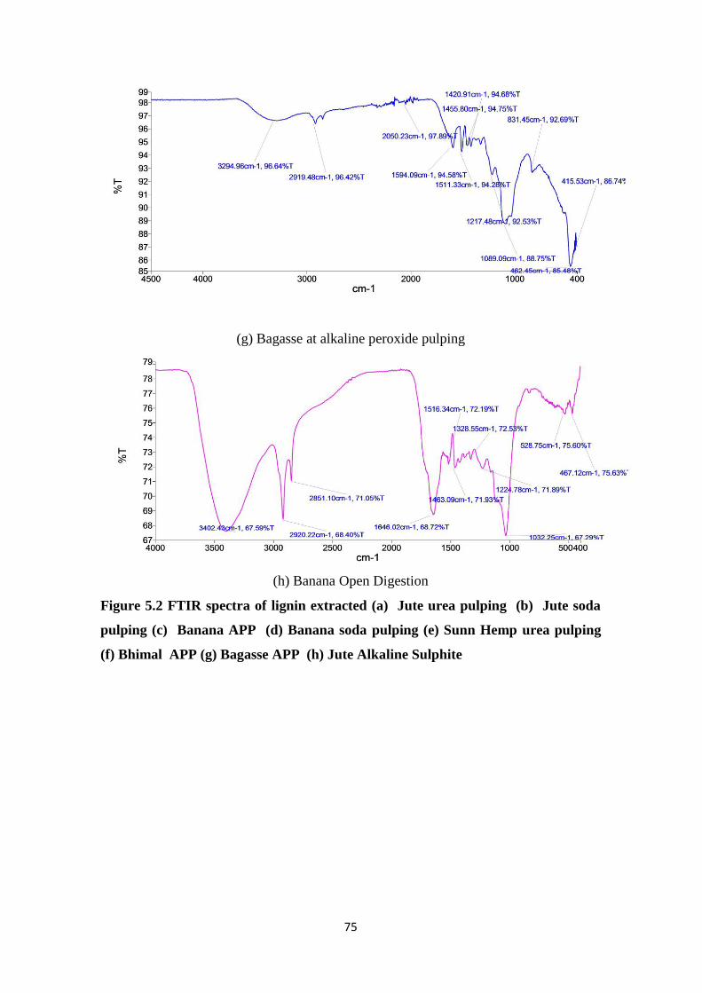
75
(g) Bagasse at alkaline peroxide pulping
(h) Banana Open Digestion
Figure 5.2 FTIR spectra of lignin extracted (a) Jute urea pulping (b) Jute soda
pulping (c) Banana APP (d) Banana soda pulping (e) Sunn Hemp urea pulping
(f) Bhimal APP (g) Bagasse APP (h) Jute Alkaline Sulphite
Internal Diameter of column=3.2 cm,
Length of column=100 cm
Capacity of peristaltic pump= 1 L/min,
Capacity of rotameter for inlet flow rate=0 to 5 LPM
Capacity of rotameter for outlet flow rate=0.1 to 1 LPM
Pressure of feed ozone= 4 psi at 2 LPM,
Capacity of inlet pressure gauge=30 psi
Capacity of outlet pressure gauge=2 psi
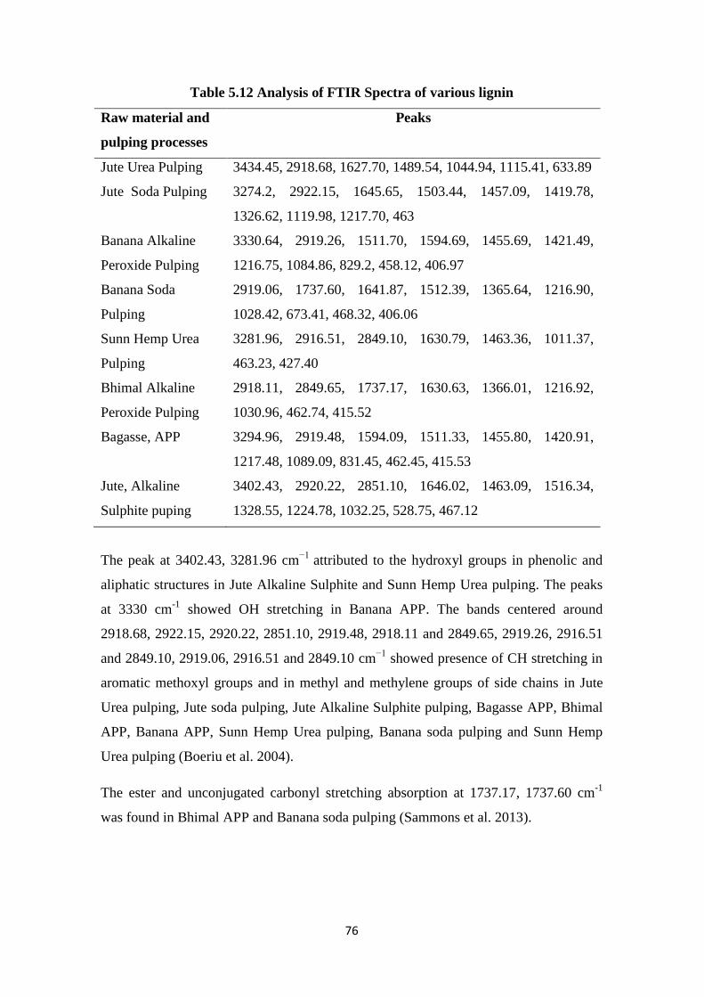
76
Table 5.12 Analysis of FTIR Spectra of various lignin
Raw material and
pulping processes
Peaks
Jute Urea Pulping 3434.45, 2918.68, 1627.70, 1489.54, 1044.94, 1115.41, 633.89
Jute Soda Pulping 3274.2, 2922.15, 1645.65, 1503.44, 1457.09, 1419.78,
1326.62, 1119.98, 1217.70, 463
Banana Alkaline
Peroxide Pulping
3330.64, 2919.26, 1511.70, 1594.69, 1455.69, 1421.49,
1216.75, 1084.86, 829.2, 458.12, 406.97
Banana Soda
Pulping
2919.06, 1737.60, 1641.87, 1512.39, 1365.64, 1216.90,
1028.42, 673.41, 468.32, 406.06
Sunn Hemp Urea
Pulping
3281.96, 2916.51, 2849.10, 1630.79, 1463.36, 1011.37,
463.23, 427.40
Bhimal Alkaline
Peroxide Pulping
2918.11, 2849.65, 1737.17, 1630.63, 1366.01, 1216.92,
1030.96, 462.74, 415.52
Bagasse, APP 3294.96, 2919.48, 1594.09, 1511.33, 1455.80, 1420.91,
1217.48, 1089.09, 831.45, 462.45, 415.53
Jute, Alkaline
Sulphite puping
3402.43, 2920.22, 2851.10, 1646.02, 1463.09, 1516.34,
1328.55, 1224.78, 1032.25, 528.75, 467.12
The peak at 3402.43, 3281.96 cm−1
attributed to the hydroxyl groups in phenolic and
aliphatic structures in Jute Alkaline Sulphite and Sunn Hemp Urea pulping. The peaks
at 3330 cm-1
showed OH stretching in Banana APP. The bands centered around
2918.68, 2922.15, 2920.22, 2851.10, 2919.48, 2918.11 and 2849.65, 2919.26, 2916.51
and 2849.10, 2919.06, 2916.51 and 2849.10 cm−1
showed presence of CH stretching in
aromatic methoxyl groups and in methyl and methylene groups of side chains in Jute
Urea pulping, Jute soda pulping, Jute Alkaline Sulphite pulping, Bagasse APP, Bhimal
APP, Banana APP, Sunn Hemp Urea pulping, Banana soda pulping and Sunn Hemp
Urea pulping (Boeriu et al. 2004).
The ester and unconjugated carbonyl stretching absorption at 1737.17, 1737.60 cm-1
was found in Bhimal APP and Banana soda pulping (Sammons et al. 2013).
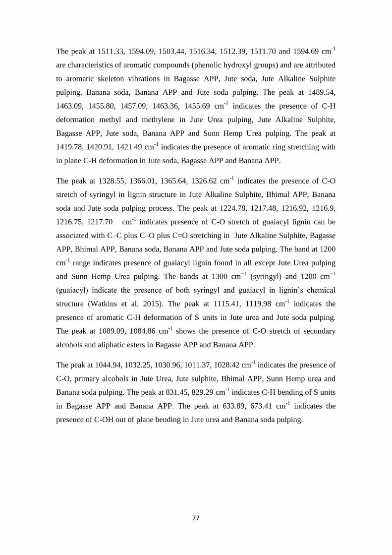
77
The peak at 1511.33, 1594.09, 1503.44, 1516.34, 1512.39, 1511.70 and 1594.69 cm-1
are characteristics of aromatic compounds (phenolic hydroxyl groups) and are attributed
to aromatic skeleton vibrations in Bagasse APP, Jute soda, Jute Alkaline Sulphite
pulping, Banana soda, Banana APP and Jute soda pulping. The peak at 1489.54,
1463.09, 1455.80, 1457.09, 1463.36, 1455.69 cm-1
indicates the presence of C-H
deformation methyl and methylene in Jute Urea pulping, Jute Alkaline Sulphite,
Bagasse APP, Jute soda, Banana APP and Sunn Hemp Urea pulping. The peak at
1419.78, 1420.91, 1421.49 cm-1
indicates the presence of aromatic ring stretching with
in plane C-H deformation in Jute soda, Bagasse APP and Banana APP.
The peak at 1328.55, 1366.01, 1365.64, 1326.62 cm-1
indicates the presence of C-O
stretch of syringyl in lignin structure in Jute Alkaline Sulphite, Bhimal APP, Banana
soda and Jute soda pulping process. The peak at 1224.78, 1217.48, 1216.92, 1216.9,
1216.75, 1217.70 cm-1
indicates presence of C-O stretch of guaiacyl lignin can be
associated with C–C plus C–O plus C=O stretching in Jute Alkaline Sulphite, Bagasse
APP, Bhimal APP, Banana soda, Banana APP and Jute soda pulping. The band at 1200
cm-1
range indicates presence of guaiacyl lignin found in all except Jute Urea pulping
and Sunn Hemp Urea pulping. The bands at 1300 cm−1
(syringyl) and 1200 cm−1
(guaiacyl) indicate the presence of both syringyl and guaiacyl in lignin’s chemical
structure (Watkins et al. 2015). The peak at 1115.41, 1119.98 cm-1
indicates the
presence of aromatic C-H deformation of S units in Jute urea and Jute soda pulping.
The peak at 1089.09, 1084.86 cm-1
shows the presence of C-O stretch of secondary
alcohols and aliphatic esters in Bagasse APP and Banana APP.
The peak at 1044.94, 1032.25, 1030.96, 1011.37, 1028.42 cm-1
indicates the presence of
C-O, primary alcohols in Jute Urea, Jute sulphite, Bhimal APP, Sunn Hemp urea and
Banana soda pulping. The peak at 831.45, 829.29 cm-1
indicates C-H bending of S units
in Bagasse APP and Banana APP. The peak at 633.89, 673.41 cm-1
indicates the
presence of C-OH out of plane bending in Jute urea and Banana soda pulping.
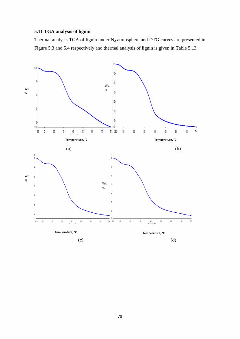
78
5.11 TGA analysis of lignin
Thermal analysis TGA of lignin under N2 atmosphere and DTG curves are presented in
Figure 5.3 and 5.4 respectively and thermal analysis of lignin is given in Table 5.13.
(a) (b)
(c) (d)
Temperature, °C Temperature, °C
Temperature, °C Temperature, °C
Wt.
%
Wt.
%
Wt.
% Wt.
%
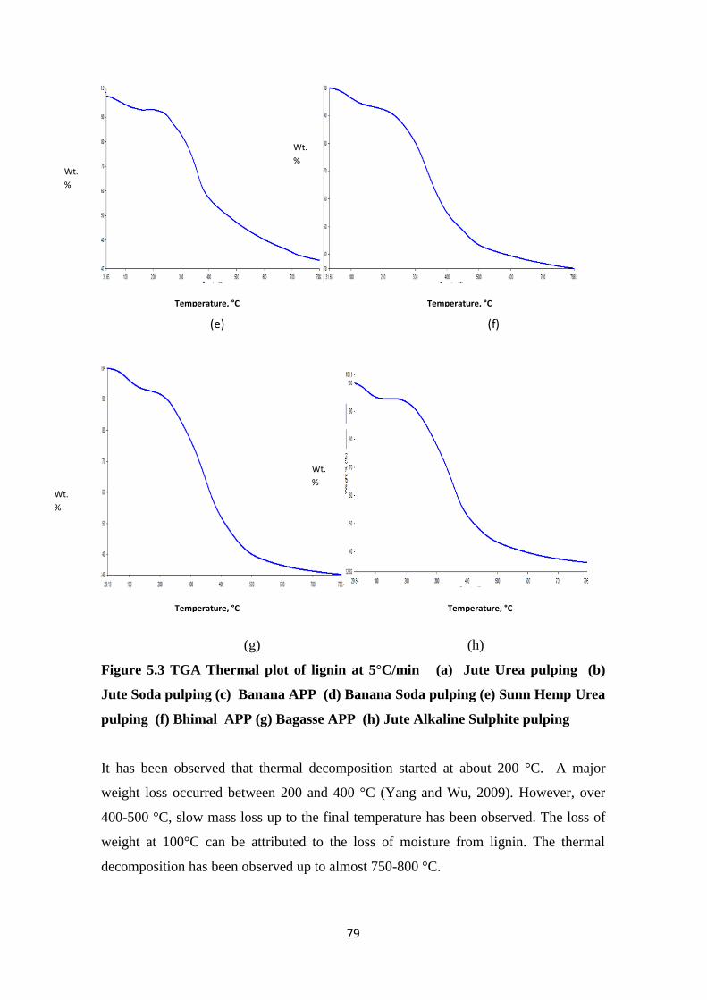
79
(e) (f)
(g) (h)
Figure 5.3 TGA Thermal plot of lignin at 5°C/min (a) Jute Urea pulping (b)
Jute Soda pulping (c) Banana APP (d) Banana Soda pulping (e) Sunn Hemp Urea
pulping (f) Bhimal APP (g) Bagasse APP (h) Jute Alkaline Sulphite pulping
It has been observed that thermal decomposition started at about 200 °C. A major
weight loss occurred between 200 and 400 °C (Yang and Wu, 2009). However, over
400-500 °C, slow mass loss up to the final temperature has been observed. The loss of
weight at 100°C can be attributed to the loss of moisture from lignin. The thermal
decomposition has been observed up to almost 750-800 °C.
Temperature, °C Temperature, °C
Temperature, °C Temperature, °C
Wt.
%
Wt.
%
Wt.
%
Wt.
%
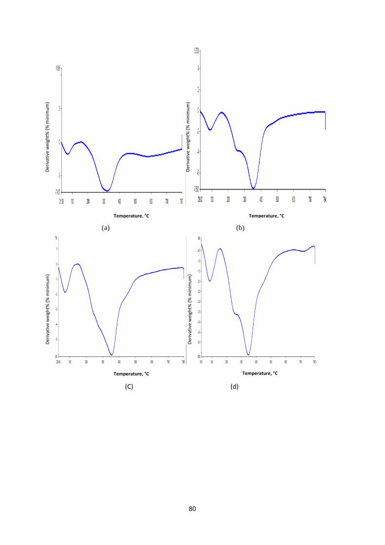
80
(a) (b)
(C) (d)
Temperature, °C Temperature, °C
Temperature, °C Temperature, °C
Der
ivat
ive
wei
ght%
(%
min
imu
m)
Der
ivat
ive
wei
ght%
(%
min
imu
m)
Der
ivat
ive
wei
ght%
(%
min
imu
m)
Der
ivat
ive
wei
ght%
(%
min
imu
m)
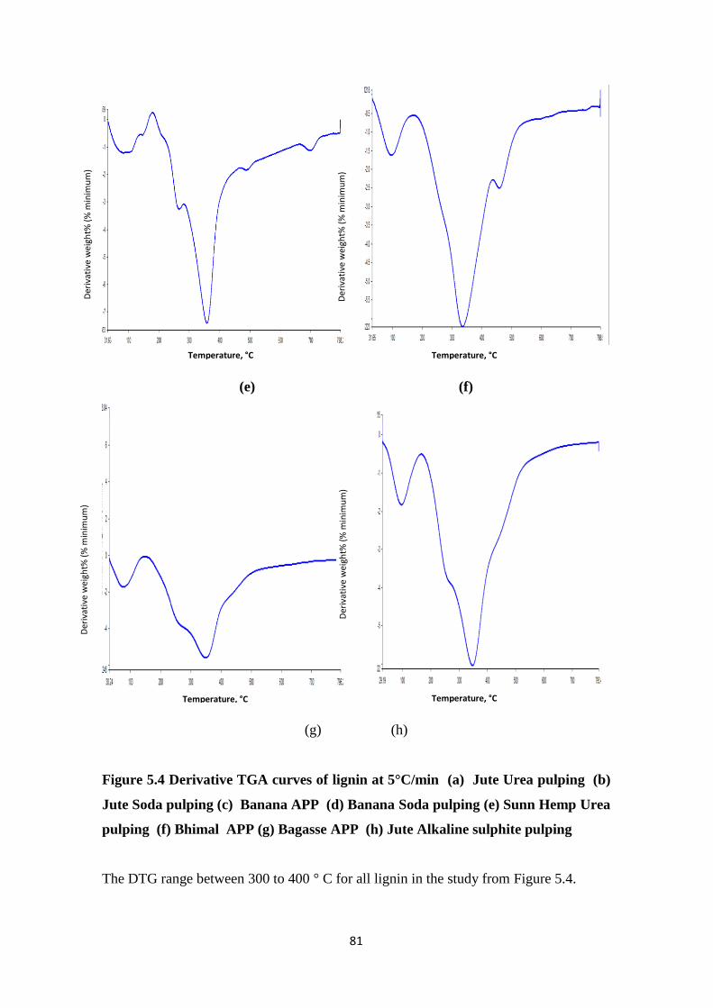
81
(e) (f)
(g) (h)
Figure 5.4 Derivative TGA curves of lignin at 5°C/min (a) Jute Urea pulping (b)
Jute Soda pulping (c) Banana APP (d) Banana Soda pulping (e) Sunn Hemp Urea
pulping (f) Bhimal APP (g) Bagasse APP (h) Jute Alkaline sulphite pulping
The DTG range between 300 to 400 ° C for all lignin in the study from Figure 5.4.
Temperature, °C Temperature, °C
Temperature, °C Temperature, °C
Der
ivat
ive
wei
ght%
(%
min
imu
m)
Der
ivat
ive
wei
ght%
(%
min
imu
m)
Der
ivat
ive
wei
ght%
(%
min
imu
m)
Der
ivat
ive
wei
ght%
(%
min
imu
m)
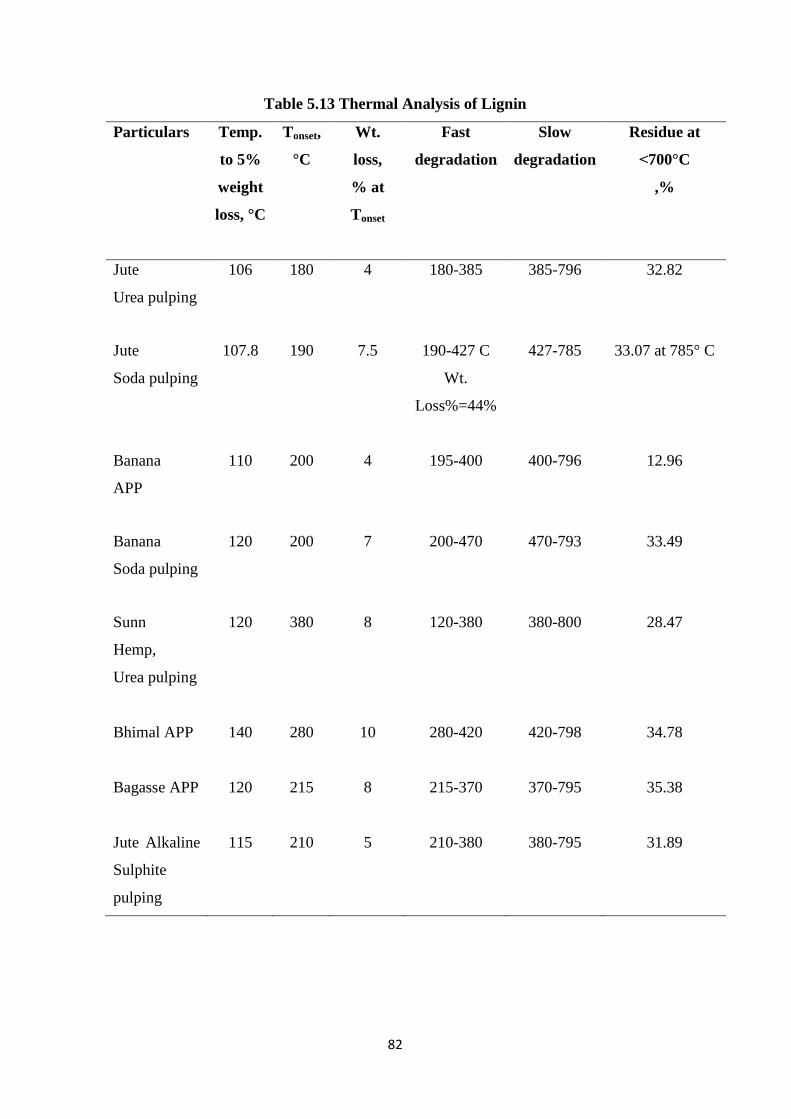
82
Table 5.13 Thermal Analysis of Lignin
Particulars Temp.
to 5%
weight
loss, °C
Tonset,
°C
Wt.
loss,
% at
Tonset
Fast
degradation
Slow
degradation
Residue at
˂700°C
,%
Jute
Urea pulping
106 180 4 180-385 385-796 32.82
Jute
Soda pulping
107.8 190 7.5 190-427 C
Wt.
Loss%=44%
427-785 33.07 at 785° C
Banana
APP
110 200 4 195-400 400-796 12.96
Banana
Soda pulping
120 200 7 200-470 470-793 33.49
Sunn
Hemp,
Urea pulping
120 380 8 120-380 380-800 28.47
Bhimal APP
140
280
10
280-420
420-798
34.78
Bagasse APP 120 215 8 215-370 370-795 35.38
Jute Alkaline
Sulphite
pulping
115
210
5
210-380
380-795
31.89
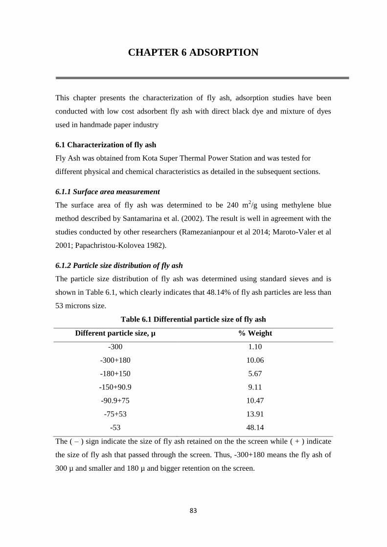
83
CHAPTER 6 ADSORPTION
This chapter presents the characterization of fly ash, adsorption studies have been
conducted with low cost adsorbent fly ash with direct black dye and mixture of dyes
used in handmade paper industry
6.1 Characterization of fly ash
Fly Ash was obtained from Kota Super Thermal Power Station and was tested for
different physical and chemical characteristics as detailed in the subsequent sections.
6.1.1 Surface area measurement
The surface area of fly ash was determined to be 240 m2/g using methylene blue
method described by Santamarina et al. (2002). The result is well in agreement with the
studies conducted by other researchers (Ramezanianpour et al 2014; Maroto-Valer et al
2001; Papachristou-Kolovea 1982).
6.1.2 Particle size distribution of fly ash
The particle size distribution of fly ash was determined using standard sieves and is
shown in Table 6.1, which clearly indicates that 48.14% of fly ash particles are less than
53 microns size.
Table 6.1 Differential particle size of fly ash
Different particle size, µ % Weight
-300 1.10
-300+180 10.06
-180+150 5.67
-150+90.9 9.11
-90.9+75 10.47
-75+53 13.91
-53 48.14
The ( – ) sign indicate the size of fly ash retained on the the screen while ( + ) indicate
the size of fly ash that passed through the screen. Thus, -300+180 means the fly ash of
300 µ and smaller and 180 µ and bigger retention on the screen.
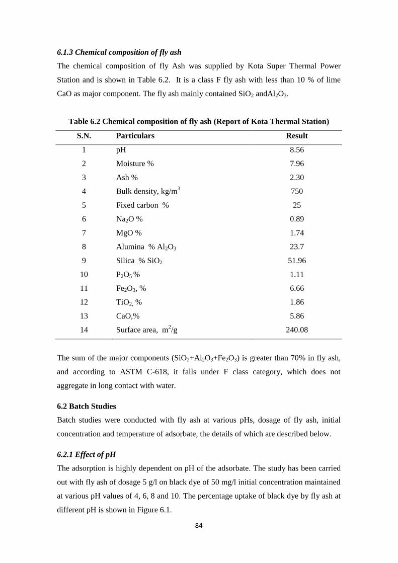
84
6.1.3 Chemical composition of fly ash
The chemical composition of fly Ash was supplied by Kota Super Thermal Power
Station and is shown in Table 6.2. It is a class F fly ash with less than 10 % of lime
CaO as major component. The fly ash mainly contained SiO2 andAl2O3.
Table 6.2 Chemical composition of fly ash (Report of Kota Thermal Station)
S.N. Particulars Result
1 pH 8.56
2 Moisture % 7.96
3 Ash % 2.30
4 Bulk density, kg/m3
750
5 Fixed carbon % 25
6 Na2O % 0.89
7 MgO % 1.74
8 Alumina % Al2O3 23.7
9 Silica % SiO2 51.96
10
11
12
13
P2O5 %
Fe2O3, %
TiO2, %
CaO,%
1.11
6.66
1.86
5.86
14 Surface area, m2/g 240.08
The sum of the major components (SiO2+Al2O3+Fe2O3) is greater than 70% in fly ash,
and according to ASTM C-618, it falls under F class category, which does not
aggregate in long contact with water.
6.2 Batch Studies
Batch studies were conducted with fly ash at various pHs, dosage of fly ash, initial
concentration and temperature of adsorbate, the details of which are described below.
6.2.1 Effect of pH
The adsorption is highly dependent on pH of the adsorbate. The study has been carried
out with fly ash of dosage 5 g/l on black dye of 50 mg/l initial concentration maintained
at various pH values of 4, 6, 8 and 10. The percentage uptake of black dye by fly ash at
different pH is shown in Figure 6.1.
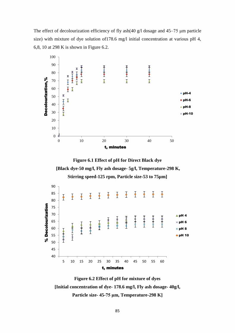
85
The effect of decolourization efficiency of fly ash(40 g/l dosage and 45–75 μm particle
size) with mixture of dye solution of178.6 mg/l initial concentration at various pH 4,
6,8, 10 at 298 K is shown in Figure 6.2.
Figure 6.1 Effect of pH for Direct Black dye
[Black dye-50 mg/l, Fly ash dosage- 5g/l, Temperature-298 K,
Stirring speed-125 rpm, Particle size-53 to 75µm]
Figure 6.2 Effect of pH for mixture of dyes
[Initial concentration of dye- 178.6 mg/l, Fly ash dosage- 40g/l,
Particle size- 45-75 μm, Temperature-298 K]
0
10
20
30
40
50
60
70
80
90
100
0 10 20 30 40 50
Decolourization,%
t, minutes
pH-4
pH-6
pH-8
pH-10
40
45
50
55
60
65
70
75
80
85
90
5 10 15 20 25 30 35 40 45 50 55 60
% D
ecolourization
t, minutes
pH 4
pH 6
pH 8
pH 10
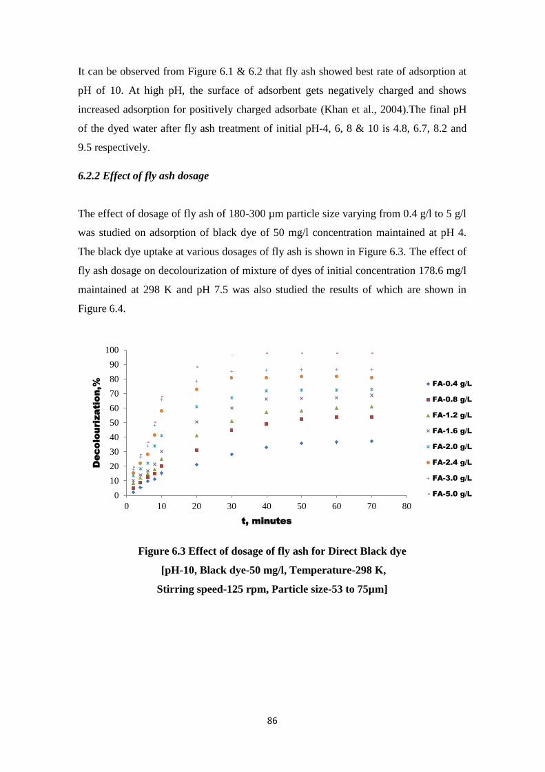
86
It can be observed from Figure 6.1 & 6.2 that fly ash showed best rate of adsorption at
pH of 10. At high pH, the surface of adsorbent gets negatively charged and shows
increased adsorption for positively charged adsorbate (Khan et al., 2004).The final pH
of the dyed water after fly ash treatment of initial pH-4, 6, 8 & 10 is 4.8, 6.7, 8.2 and
9.5 respectively.
6.2.2 Effect of fly ash dosage
The effect of dosage of fly ash of 180-300 µm particle size varying from 0.4 g/l to 5 g/l
was studied on adsorption of black dye of 50 mg/l concentration maintained at pH 4.
The black dye uptake at various dosages of fly ash is shown in Figure 6.3. The effect of
fly ash dosage on decolourization of mixture of dyes of initial concentration 178.6 mg/l
maintained at 298 K and pH 7.5 was also studied the results of which are shown in
Figure 6.4.
Figure 6.3 Effect of dosage of fly ash for Direct Black dye
[pH-10, Black dye-50 mg/l, Temperature-298 K,
Stirring speed-125 rpm, Particle size-53 to 75µm]
0
10
20
30
40
50
60
70
80
90
100
0 10 20 30 40 50 60 70 80
Decolourization,%
t, minutes
FA-0.4 g/L
FA-0.8 g/L
FA-1.2 g/L
FA-1.6 g/L
FA-2.0 g/L
FA-2.4 g/L
FA-3.0 g/L
FA-5.0 g/L
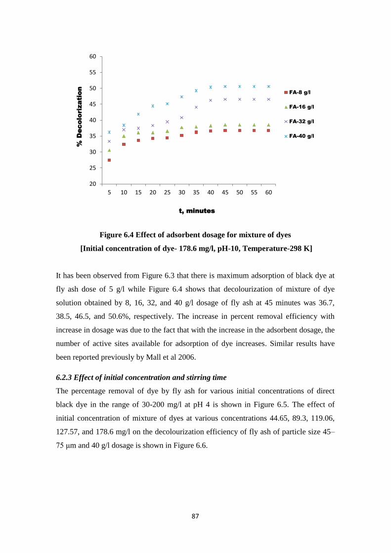
87
Figure 6.4 Effect of adsorbent dosage for mixture of dyes
[Initial concentration of dye- 178.6 mg/l, pH-10, Temperature-298 K]
It has been observed from Figure 6.3 that there is maximum adsorption of black dye at
fly ash dose of 5 g/l while Figure 6.4 shows that decolourization of mixture of dye
solution obtained by 8, 16, 32, and 40 g/l dosage of fly ash at 45 minutes was 36.7,
38.5, 46.5, and 50.6%, respectively. The increase in percent removal efficiency with
increase in dosage was due to the fact that with the increase in the adsorbent dosage, the
number of active sites available for adsorption of dye increases. Similar results have
been reported previously by Mall et al 2006.
6.2.3 Effect of initial concentration and stirring time
The percentage removal of dye by fly ash for various initial concentrations of direct
black dye in the range of 30-200 mg/l at pH 4 is shown in Figure 6.5. The effect of
initial concentration of mixture of dyes at various concentrations 44.65, 89.3, 119.06,
127.57, and 178.6 mg/l on the decolourization efficiency of fly ash of particle size 45–
75 μm and 40 g/l dosage is shown in Figure 6.6.
20
25
30
35
40
45
50
55
60
5 10 15 20 25 30 35 40 45 50 55 60
% D
ecolorization
t, minutes
FA-8 g/l
FA-16 g/l
FA-32 g/l
FA-40 g/l
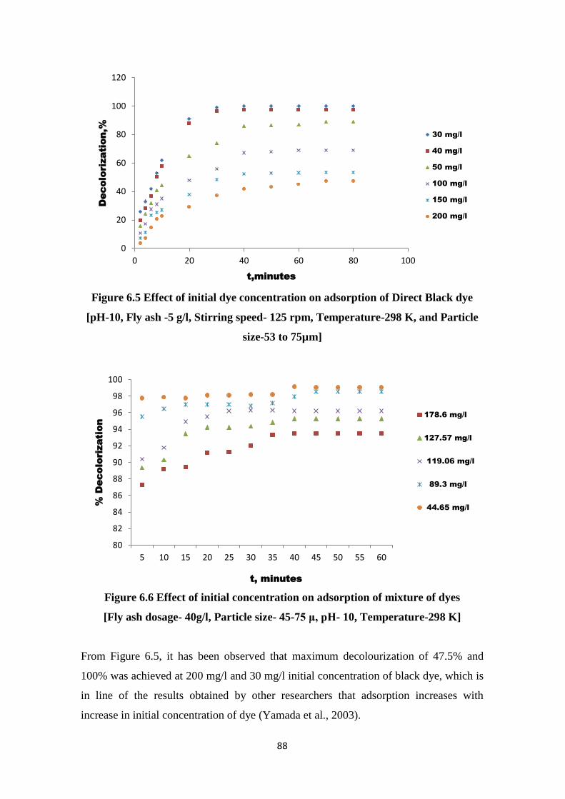
88
Figure 6.5 Effect of initial dye concentration on adsorption of Direct Black dye
[pH-10, Fly ash -5 g/l, Stirring speed- 125 rpm, Temperature-298 K, and Particle
size-53 to 75µm]
Figure 6.6 Effect of initial concentration on adsorption of mixture of dyes
[Fly ash dosage- 40g/l, Particle size- 45-75 μ, pH- 10, Temperature-298 K]
From Figure 6.5, it has been observed that maximum decolourization of 47.5% and
100% was achieved at 200 mg/l and 30 mg/l initial concentration of black dye, which is
in line of the results obtained by other researchers that adsorption increases with
increase in initial concentration of dye (Yamada et al., 2003).
0
20
40
60
80
100
120
0 20 40 60 80 100
Decolorization,%
t,minutes
30 mg/l
40 mg/l
50 mg/l
100 mg/l
150 mg/l
200 mg/l
80
82
84
86
88
90
92
94
96
98
100
5 10 15 20 25 30 35 40 45 50 55 60
% D
ecolorization
t, minutes
178.6 mg/l
127.57 mg/l
119.06 mg/l
89.3 mg/l
44.65 mg/l
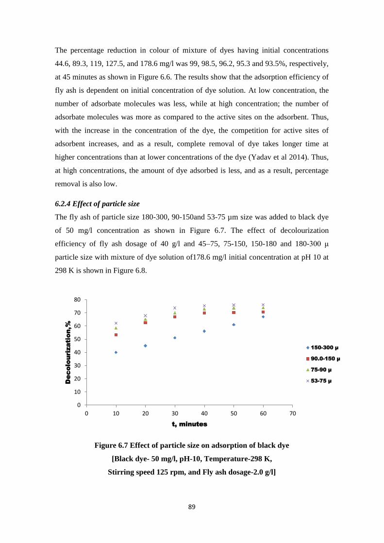
89
The percentage reduction in colour of mixture of dyes having initial concentrations
44.6, 89.3, 119, 127.5, and 178.6 mg/l was 99, 98.5, 96.2, 95.3 and 93.5%, respectively,
at 45 minutes as shown in Figure 6.6. The results show that the adsorption efficiency of
fly ash is dependent on initial concentration of dye solution. At low concentration, the
number of adsorbate molecules was less, while at high concentration; the number of
adsorbate molecules was more as compared to the active sites on the adsorbent. Thus,
with the increase in the concentration of the dye, the competition for active sites of
adsorbent increases, and as a result, complete removal of dye takes longer time at
higher concentrations than at lower concentrations of the dye (Yadav et al 2014). Thus,
at high concentrations, the amount of dye adsorbed is less, and as a result, percentage
removal is also low.
6.2.4 Effect of particle size
The fly ash of particle size 180-300, 90-150and 53-75 µm size was added to black dye
of 50 mg/l concentration as shown in Figure 6.7. The effect of decolourization
efficiency of fly ash dosage of 40 g/l and 45–75, 75-150, 150-180 and 180-300 μ
particle size with mixture of dye solution of178.6 mg/l initial concentration at pH 10 at
298 K is shown in Figure 6.8.
Figure 6.7 Effect of particle size on adsorption of black dye
[Black dye- 50 mg/l, pH-10, Temperature-298 K,
Stirring speed 125 rpm, and Fly ash dosage-2.0 g/l]
0
10
20
30
40
50
60
70
80
0 10 20 30 40 50 60 70
Decolourization,%
t, minutes
150-300 µ
90.0-150 µ
75-90 µ
53-75 µ

90
Figure 6.8 Effect of particle size of adsorbent
[Initial concentration of dye-178.6 mg/l,
Fly ash dosage-40g/l, pH- 7.5, Temperature-298 K]
It is observed from Figure 6.7 & 6.8 that maximum adsorption rate of black dye was
achieved with fly ash of smallest size 53-75 µ with percentage reduction of 76% while
maximum percentage reduction in colour of mixture of dyes obtained by fly ash of
particle size 45–75 μ was 55.7% at 45 minutes. The decolourization of dye solution
increased with the decrease in the particle size of fly ash because smaller particles have
relatively larger surface area and therefore offer more adsorption sites. Similar results
have been reported by Kara et al., Gupta et al., 1988. The presence of more than one
dye showed less reduction in comparison to single dye i.e. black dye. It may be due to
competitive adsorption onto adsorption sites. The attraction of dye to the interfaces of
adsorbent is different for each dye and therefore, the presence of mixture of dyes
enhances competitive adsorption (Regti et al. 2016).
6.2.5 Effect of temperature
The effect of various temperature of dye solution, i.e. 20, 25, 30, 35 and 40°C on
decolourization efficiency of black dye solution of initial concentration of 178.6 mg/L
maintained at pH 4is shown in Figure 6.9.
30
35
40
45
50
55
60
5 10 15 20 25 30 35 40 45 50 55 60
% D
ecolourization
t, minutes
180-300µ
150-180µ
75-150µ
45-75µ
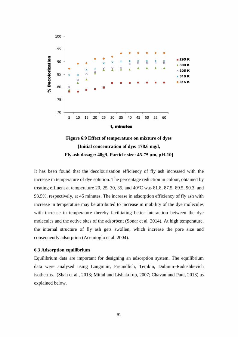
91
Figure 6.9 Effect of temperature on mixture of dyes
[Initial concentration of dye: 178.6 mg/l,
Fly ash dosage: 40g/l, Particle size: 45-75 μm, pH-10]
It has been found that the decolourization efficiency of fly ash increased with the
increase in temperature of dye solution. The percentage reduction in colour, obtained by
treating effluent at temperature 20, 25, 30, 35, and 40°C was 81.8, 87.5, 89.5, 90.3, and
93.5%, respectively, at 45 minutes. The increase in adsorption efficiency of fly ash with
increase in temperature may be attributed to increase in mobility of the dye molecules
with increase in temperature thereby facilitating better interaction between the dye
molecules and the active sites of the adsorbent (Sonar et al. 2014). At high temperature,
the internal structure of fly ash gets swollen, which increase the pore size and
consequently adsorption (Acemioglu et al. 2004).
6.3 Adsorption equilibrium
Equilibrium data are important for designing an adsorption system. The equilibrium
data were analysed using Langmuir, Freundlich, Temkin, Dubinin–Radushkevich
isotherms. (Shah et al., 2013; Mittal and Lishakurup, 2007; Chavan and Paul, 2013) as
explained below.
70
75
80
85
90
95
100
5 10 15 20 25 30 35 40 45 50 55 60
% D
ecolorization
t, minutes
295 K
300 K
305 K
310 K
315 K
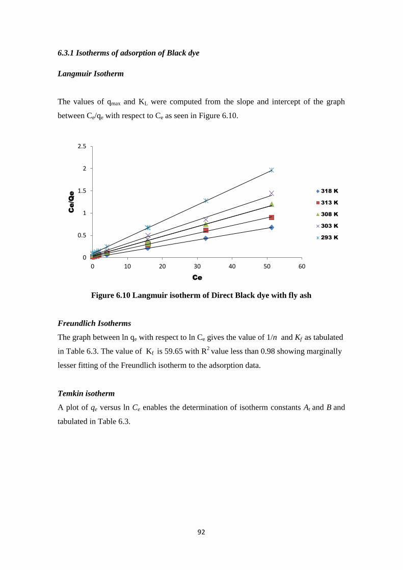
92
6.3.1 Isotherms of adsorption of Black dye
Langmuir Isotherm
The values of qmax and KL were computed from the slope and intercept of the graph
between Ce/qe with respect to Ce as seen in Figure 6.10.
Figure 6.10 Langmuir isotherm of Direct Black dye with fly ash
Freundlich Isotherms
The graph between ln qe with respect to ln Ce gives the value of 1/n and Kf as tabulated
in Table 6.3. The value of Kf is 59.65 with R2
value less than 0.98 showing marginally
lesser fitting of the Freundlich isotherm to the adsorption data.
Temkin isotherm
A plot of qe versus ln Ce enables the determination of isotherm constants At and B and
tabulated in Table 6.3.
0
0.5
1
1.5
2
2.5
0 10 20 30 40 50 60
Ce/Q
e
Ce
318 K
313 K
308 K
303 K
293 K
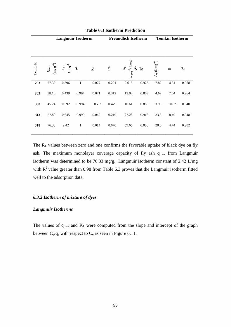
93
Table 6.3 Isotherm Prediction
Langmuir Isotherm Freundlich Isotherm Temkin Isotherm T
emp
, K
Qm
ax
(mg
g-1
)
KL
L m
g-1
R2
RL
1/n
Kf
(mgm
g-1
(Lm
g-
1)1
/n
R2
AT
(L
mg
-1)
B
R2
293 27.39 0.396 1 0.077 0.291 9.615 0.923 7.82 4.81 0.968
303 38.16 0.439 0.994 0.071 0.312 13.03 0.863 4.62 7.64 0.964
308 45.24 0.592 0.994 0.0533 0.479 10.61 0.880 3.95 10.82 0.940
313 57.80 0.645 0.999 0.049 0.210 27.28 0.916 23.6 8.40 0.948
318 76.33 2.42 1 0.014 0.070 59.65 0.886 28.6 4.74 0.902
The RL values between zero and one confirms the favorable uptake of black dye on fly
ash. The maximum monolayer coverage capacity of fly ash qmax from Langmuir
isotherm was determined to be 76.33 mg/g. Langmuir isotherm constant of 2.42 L/mg
with R2
value greater than 0.98 from Table 6.3 proves that the Langmuir isotherm fitted
well to the adsorption data.
6.3.2 Isotherm of mixture of dyes
Langmuir Isotherms
The values of qmax and KL were computed from the slope and intercept of the graph
between Ce/qe with respect to Ce as seen in Figure 6.11.
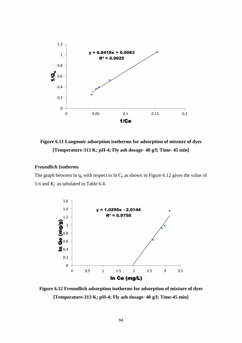
94
Figure 6.11 Langmuir adsorption isotherms for adsorption of mixture of dyes
[Temperature-313 K; pH-4; Fly ash dosage- 40 g/l; Time- 45 min]
Freundlich Isotherms
The graph between ln qe with respect to ln Ce as shown in Figure 6.12 gives the value of
1/n and Kf as tabulated in Table 6.4.
Figure 6.12 Freundlich adsorption isotherms for adsorption of mixture of dyes
[Temperature-313 K; pH-4; Fly ash dosage- 40 g/l; Time-45 min]
y = 6.8418x + 0.0083
R² = 0.9925
0
0.2
0.4
0.6
0.8
1
1.2
0 0.05 0.1 0.15 0.2
1/Q
e
1/Ce
y = 1.0295x - 2.0144
R² = 0.9758
0
0.2
0.4
0.6
0.8
1
1.2
1.4
1.6
0 0.5 1 1.5 2 2.5 3 3.5
ln
Q
e (m
g/g
)
ln Ce (mg/L)
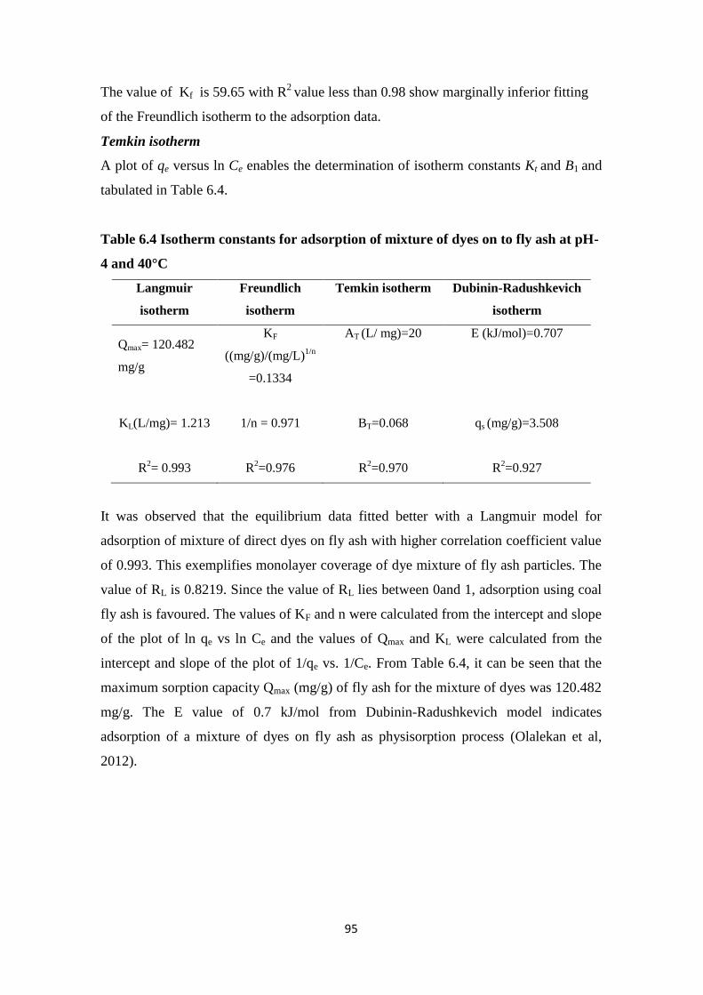
95
The value of Kf is 59.65 with R2
value less than 0.98 show marginally inferior fitting
of the Freundlich isotherm to the adsorption data.
Temkin isotherm
A plot of qe versus ln Ce enables the determination of isotherm constants Kt and B1 and
tabulated in Table 6.4.
Table 6.4 Isotherm constants for adsorption of mixture of dyes on to fly ash at pH-
4 and 40°C
Langmuir
isotherm
Freundlich
isotherm
Temkin isotherm Dubinin-Radushkevich
isotherm
Qmax= 120.482
mg/g
KF
((mg/g)/(mg/L)1/n
=0.1334
AT (L/ mg)=20 E (kJ/mol)=0.707
KL(L/mg)= 1.213
1/n = 0.971
BT=0.068
qs (mg/g)=3.508
R2= 0.993
R2=0.976
R2=0.970
R2=0.927
It was observed that the equilibrium data fitted better with a Langmuir model for
adsorption of mixture of direct dyes on fly ash with higher correlation coefficient value
of 0.993. This exemplifies monolayer coverage of dye mixture of fly ash particles. The
value of RL is 0.8219. Since the value of RL lies between 0and 1, adsorption using coal
fly ash is favoured. The values of KF and n were calculated from the intercept and slope
of the plot of ln qe vs ln Ce and the values of Qmax and KL were calculated from the
intercept and slope of the plot of 1/qe vs. 1/Ce. From Table 6.4, it can be seen that the
maximum sorption capacity Qmax (mg/g) of fly ash for the mixture of dyes was 120.482
mg/g. The E value of 0.7 kJ/mol from Dubinin-Radushkevich model indicates
adsorption of a mixture of dyes on fly ash as physisorption process (Olalekan et al,
2012).
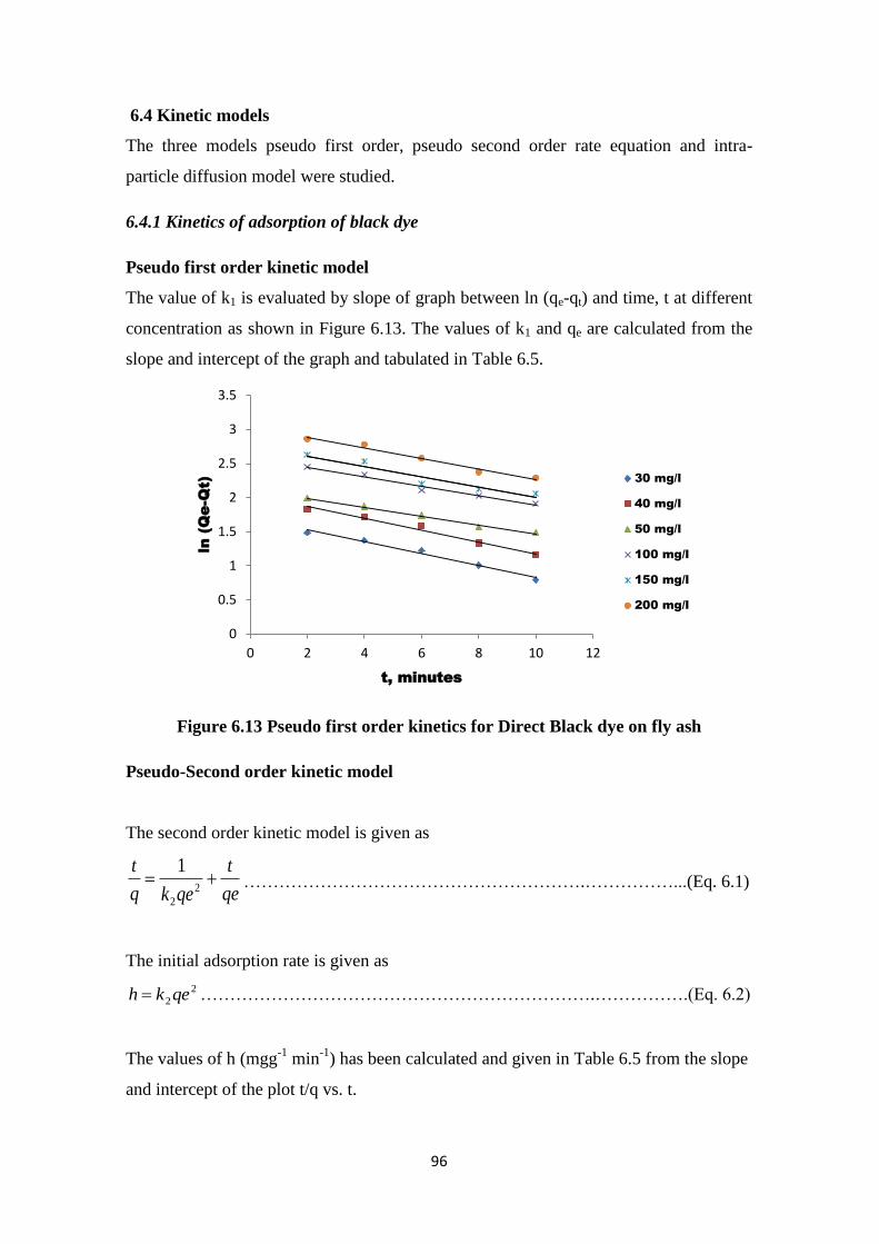
96
6.4 Kinetic models
The three models pseudo first order, pseudo second order rate equation and intra-
particle diffusion model were studied.
6.4.1 Kinetics of adsorption of black dye
Pseudo first order kinetic model
The value of k1 is evaluated by slope of graph between ln (qe-qt) and time, t at different
concentration as shown in Figure 6.13. The values of k1 and qe are calculated from the
slope and intercept of the graph and tabulated in Table 6.5.
Figure 6.13 Pseudo first order kinetics for Direct Black dye on fly ash
Pseudo-Second order kinetic model
The second order kinetic model is given as
qe
t
qekq
t
2
2
1………………………………………………….……………...(Eq. 6.1)
The initial adsorption rate is given as
2
2qekh ………………………………………………………….…………….(Eq. 6.2)
The values of h (mgg-1
min-1
) has been calculated and given in Table 6.5 from the slope
and intercept of the plot t/q vs. t.
0
0.5
1
1.5
2
2.5
3
3.5
0 2 4 6 8 10 12
ln (Q
e-Q
t)
t, minutes
30 mg/l
40 mg/l
50 mg/l
100 mg/l
150 mg/l
200 mg/l
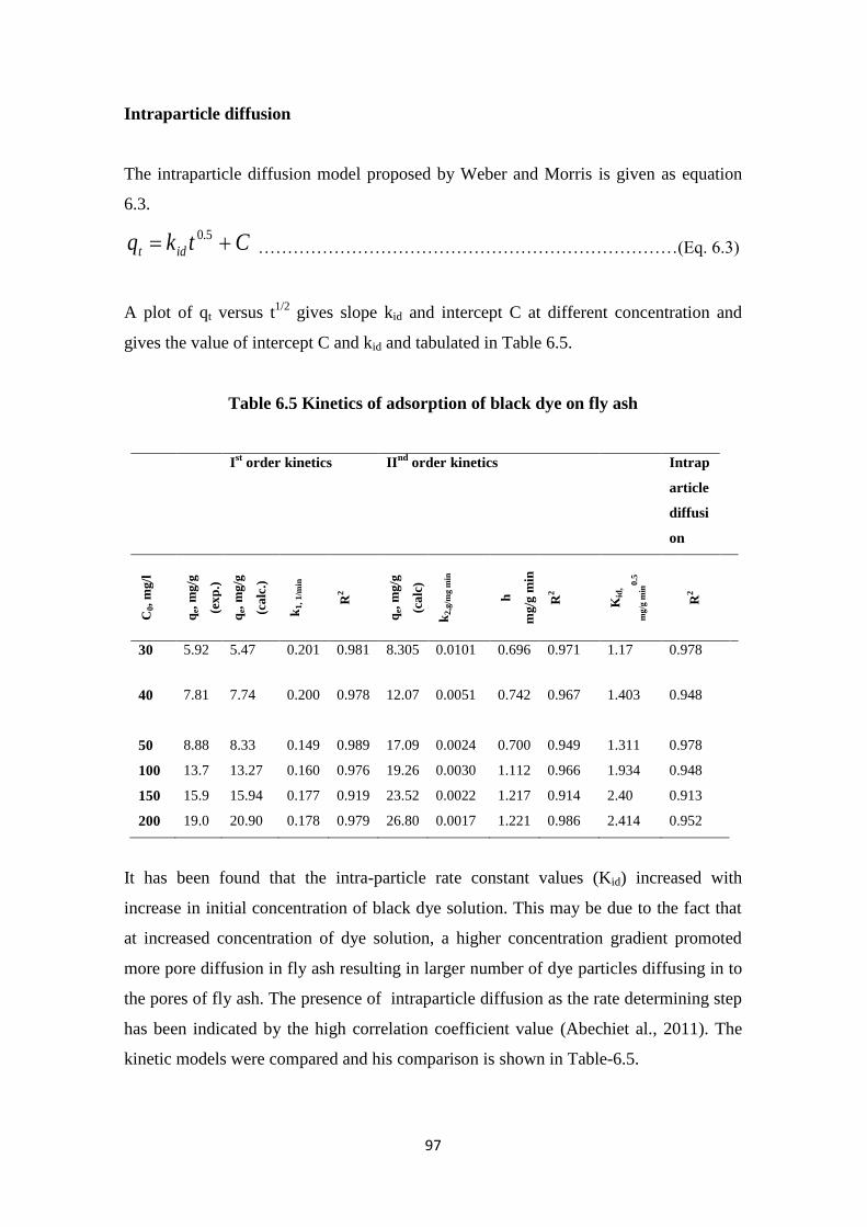
97
Intraparticle diffusion
The intraparticle diffusion model proposed by Weber and Morris is given as equation
6.3.
Ctkq idt 5.0 ………………………………………………………………(Eq. 6.3)
A plot of qt versus t1/2
gives slope kid and intercept C at different concentration and
gives the value of intercept C and kid and tabulated in Table 6.5.
Table 6.5 Kinetics of adsorption of black dye on fly ash
Ist order kinetics II
nd order kinetics Intrap
article
diffusi
on
C0,
mg/l
qe,
mg
/g
(ex
p.)
qe,
mg
/g
(ca
lc.)
k
1,
1/m
in
R2
qe,
mg
/g
(ca
lc)
k2,g
/mg m
in
h
mg
/g m
in
R2
Kid
,
mg/g
min
0.5
R2
30 5.92 5.47 0.201 0.981 8.305 0.0101 0.696 0.971 1.17 0.978
40 7.81
7.74 0.200 0.978 12.07 0.0051 0.742 0.967 1.403 0.948
50 8.88 8.33 0.149 0.989 17.09 0.0024 0.700 0.949 1.311 0.978
100 13.7 13.27 0.160 0.976 19.26 0.0030 1.112 0.966 1.934 0.948
150 15.9 15.94 0.177 0.919 23.52 0.0022 1.217 0.914 2.40 0.913
200 19.0 20.90 0.178 0.979 26.80 0.0017 1.221 0.986 2.414 0.952
It has been found that the intra-particle rate constant values (Kid) increased with
increase in initial concentration of black dye solution. This may be due to the fact that
at increased concentration of dye solution, a higher concentration gradient promoted
more pore diffusion in fly ash resulting in larger number of dye particles diffusing in to
the pores of fly ash. The presence of intraparticle diffusion as the rate determining step
has been indicated by the high correlation coefficient value (Abechiet al., 2011). The
kinetic models were compared and his comparison is shown in Table-6.5.
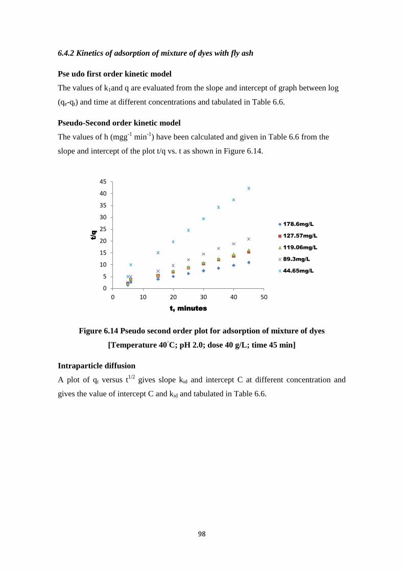
98
6.4.2 Kinetics of adsorption of mixture of dyes with fly ash
Pse udo first order kinetic model
The values of k1and q are evaluated from the slope and intercept of graph between log
(qe-qt) and time at different concentrations and tabulated in Table 6.6.
Pseudo-Second order kinetic model
The values of h (mgg-1
min-1
) have been calculated and given in Table 6.6 from the
slope and intercept of the plot t/q vs. t as shown in Figure 6.14.
Figure 6.14 Pseudo second order plot for adsorption of mixture of dyes
[Temperature 40◦C; pH 2.0; dose 40 g/L; time 45 min]
Intraparticle diffusion
A plot of qt versus t1/2
gives slope kid and intercept C at different concentration and
gives the value of intercept C and kid and tabulated in Table 6.6.
0
5
10
15
20
25
30
35
40
45
0 10 20 30 40 50
t/q
t, minutes
178.6mg/L
127.57mg/L
119.06mg/L
89.3mg/L
44.65mg/L
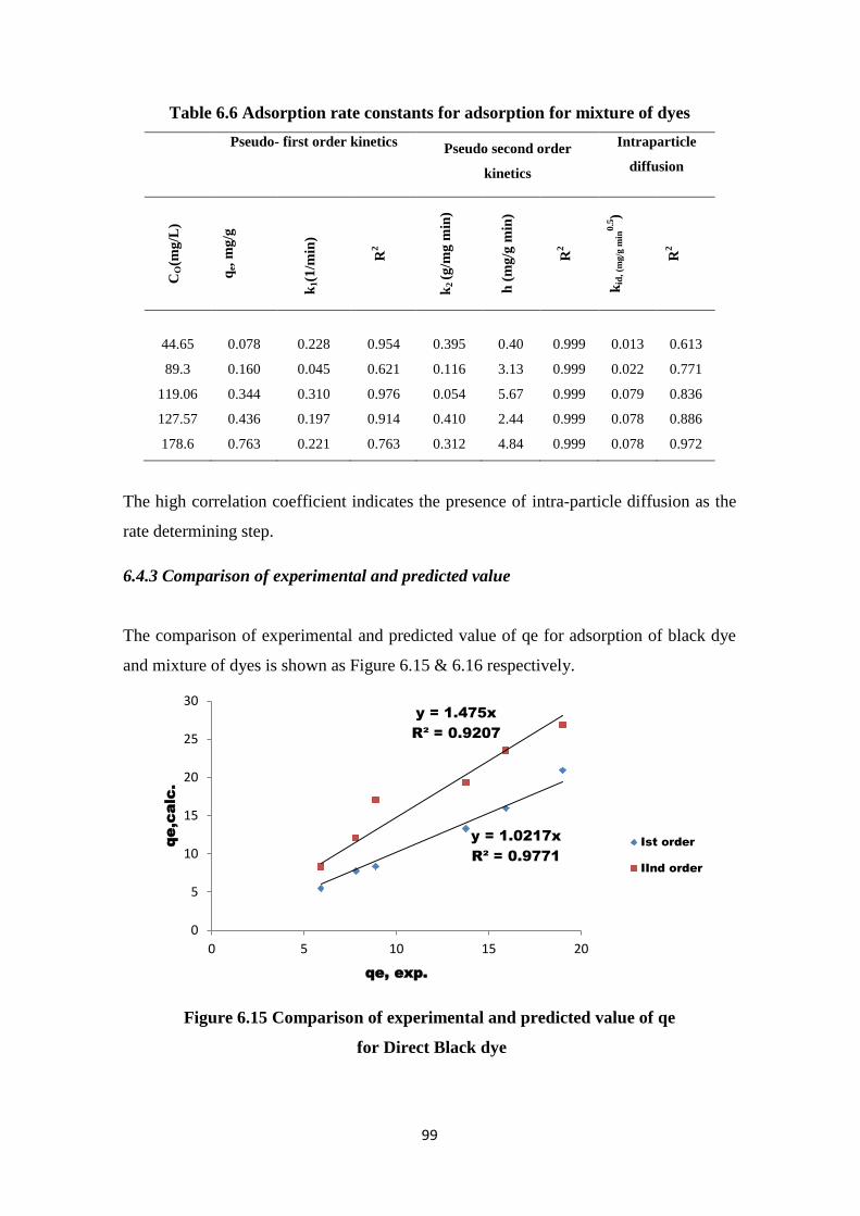
99
Table 6.6 Adsorption rate constants for adsorption for mixture of dyes
Pseudo- first order kinetics Pseudo second order
kinetics
Intraparticle
diffusion C
O(m
g/L
)
qe,
mg
/g
k
1(1
/min
)
R2
k2 (
g/m
g m
in)
h (
mg
/g m
in)
R2
kid
, (m
g/g
min
0.5)
R2
44.65
0.078
0.228
0.954
0.395
0.40
0.999
0.013
0.613
89.3 0.160 0.045 0.621 0.116 3.13 0.999 0.022 0.771
119.06 0.344 0.310 0.976 0.054 5.67 0.999 0.079 0.836
127.57 0.436 0.197 0.914 0.410 2.44 0.999 0.078 0.886
178.6 0.763 0.221 0.763 0.312 4.84 0.999 0.078 0.972
The high correlation coefficient indicates the presence of intra-particle diffusion as the
rate determining step.
6.4.3 Comparison of experimental and predicted value
The comparison of experimental and predicted value of qe for adsorption of black dye
and mixture of dyes is shown as Figure 6.15 & 6.16 respectively.
Figure 6.15 Comparison of experimental and predicted value of qe
for Direct Black dye
y = 1.0217x
R² = 0.9771
y = 1.475x
R² = 0.9207
0
5
10
15
20
25
30
0 5 10 15 20
qe,calc.
qe, exp.
Ist order
IInd order
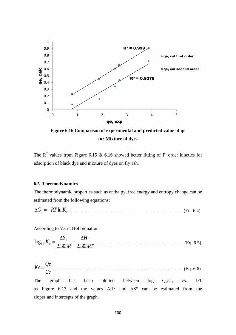
100
Figure 6.16 Comparison of experimental and predicted value of qe
for Mixture of dyes
The R2 values from Figure 6.15 & 6.16 showed better fitting of I
st order kinetics for
adsorption of black dye and mixture of dyes on fly ash.
6.5 Thermodynamics
The thermodynamic properties such as enthalpy, free energy and entropy change can be
estimated from the following equations:
cKRTG ln0 ……………………………………………………………….(Eq. 6.4)
According to Van’t Hoff equation
RT
H
R
SK c
303.2303.2log 00
10
………………………………………...………(Eq. 6.5)
Ce
QeKc ………………………………………………………………………...(Eq. 6.6)
The graph has been plotted between log Qe/Ce vs. 1/T
as Figure 6.17 and the values ΔH° and ΔS° can be estimated from the
slopes and intercepts of the graph.
R² = 0.9378
R² = 0.999
0
0.1
0.2
0.3
0.4
0.5
0.6
0.7
0.8
0.9
1
0 1 2 3 4 5
qe, calc
qe, exp
qe, cal first order
qe, cal second order
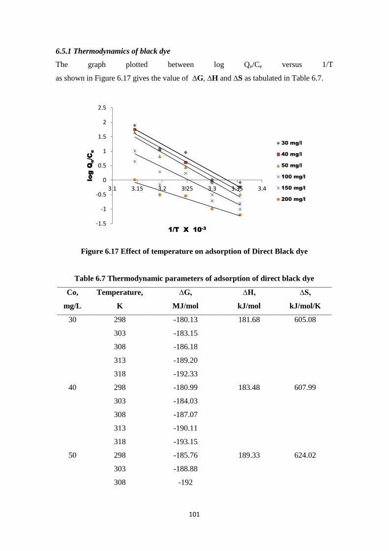
101
6.5.1 Thermodynamics of black dye
The graph plotted between log Qe/Ce versus 1/T
as shown in Figure 6.17 gives the value of ∆G, ∆H and ∆S as tabulated in Table 6.7.
Figure 6.17 Effect of temperature on adsorption of Direct Black dye
Table 6.7 Thermodynamic parameters of adsorption of direct black dye
Co,
mg/L
Temperature,
K
∆G,
MJ/mol
∆H,
kJ/mol
∆S,
kJ/mol/K
30 298 -180.13 181.68 605.08
303 -183.15
308 -186.18
313 -189.20
318 -192.33
40 298 -180.99 183.48 607.99
303 -184.03
308 -187.07
313 -190.11
318 -193.15
50 298 -185.76 189.33 624.02
303 -188.88
308 -192
-1.5
-1
-0.5
0
0.5
1
1.5
2
2.5
3.1 3.15 3.2 3.25 3.3 3.35 3.4
log Q
e/C
e
1/T X 10-3
30 mg/l
40 mg/l
50 mg/l
100 mg/l
150 mg/l
200 mg/l
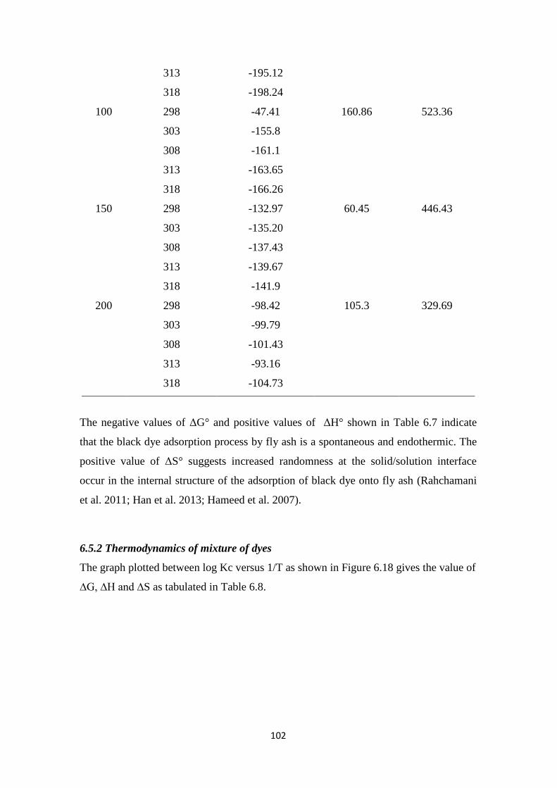
102
313 -195.12
318 -198.24
100 298 -47.41 160.86 523.36
303 -155.8
308 -161.1
313 -163.65
318 -166.26
150 298 -132.97 60.45 446.43
303 -135.20
308 -137.43
313 -139.67
318 -141.9
200 298 -98.42 105.3 329.69
303 -99.79
308 -101.43
313 -93.16
318 -104.73
The negative values of ΔG° and positive values of ΔH° shown in Table 6.7 indicate
that the black dye adsorption process by fly ash is a spontaneous and endothermic. The
positive value of ΔS° suggests increased randomness at the solid/solution interface
occur in the internal structure of the adsorption of black dye onto fly ash (Rahchamani
et al. 2011; Han et al. 2013; Hameed et al. 2007).
6.5.2 Thermodynamics of mixture of dyes
The graph plotted between log Kc versus 1/T as shown in Figure 6.18 gives the value of
∆G, ∆H and ∆S as tabulated in Table 6.8.
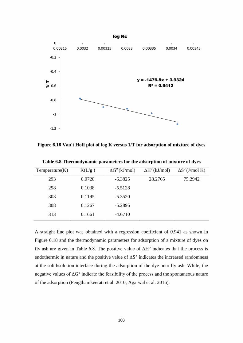
103
Figure 6.18 Van't Hoff plot of log K versus 1/T for adsorption of mixture of dyes
Table 6.8 Thermodynamic parameters for the adsorption of mixture of dyes
Temperature(K) K(L/g ) ΔGo (kJ/mol) ΔH
o (kJ/mol) ΔS
o (J/mol K)
293 0.0728 -6.3825 28.2765 75.2942
298 0.1038 -5.5128
303 0.1195 -5.3520
308 0.1267 -5.2895
313 0.1661 -4.6710
A straight line plot was obtained with a regression coefficient of 0.941 as shown in
Figure 6.18 and the thermodynamic parameters for adsorption of a mixture of dyes on
fly ash are given in Table 6.8. The positive value of ΔH° indicates that the process is
endothermic in nature and the positive value of ΔS° indicates the increased randomness
at the solid/solution interface during the adsorption of the dye onto fly ash. While, the
negative values of ΔG° indicate the feasibility of the process and the spontaneous nature
of the adsorption (Pengthamkeerati et al. 2010; Agarwal et al. 2016).
y = -1476.8x + 3.9324
R² = 0.9412
-1.2
-1
-0.8
-0.6
-0.4
-0.2
0
0.00315 0.0032 0.00325 0.0033 0.00335 0.0034 0.003451/ T
log Kc
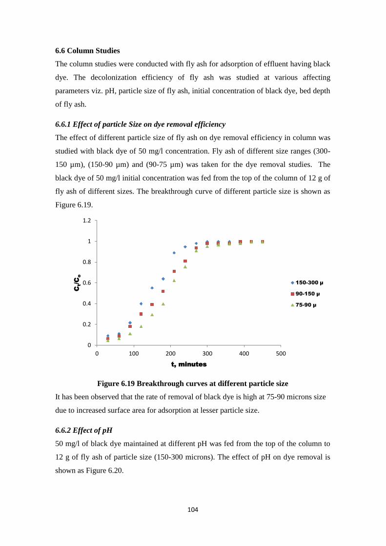
104
6.6 Column Studies
The column studies were conducted with fly ash for adsorption of effluent having black
dye. The decolonization efficiency of fly ash was studied at various affecting
parameters viz. pH, particle size of fly ash, initial concentration of black dye, bed depth
of fly ash.
6.6.1 Effect of particle Size on dye removal efficiency
The effect of different particle size of fly ash on dye removal efficiency in column was
studied with black dye of 50 mg/l concentration. Fly ash of different size ranges (300-
150 µm), (150-90 µm) and (90-75 µm) was taken for the dye removal studies. The
black dye of 50 mg/l initial concentration was fed from the top of the column of 12 g of
fly ash of different sizes. The breakthrough curve of different particle size is shown as
Figure 6.19.
Figure 6.19 Breakthrough curves at different particle size
It has been observed that the rate of removal of black dye is high at 75-90 microns size
due to increased surface area for adsorption at lesser particle size.
6.6.2 Effect of pH
50 mg/l of black dye maintained at different pH was fed from the top of the column to
12 g of fly ash of particle size (150-300 microns). The effect of pH on dye removal is
shown as Figure 6.20.
0
0.2
0.4
0.6
0.8
1
1.2
0 100 200 300 400 500
Ct/C
o
t, minutes
150-300 μ
90-150 μ
75-90 μ
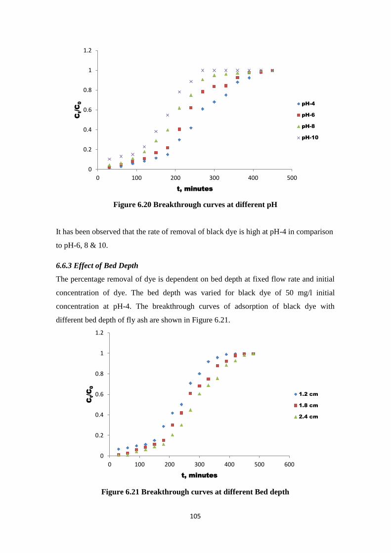
105
Figure 6.20 Breakthrough curves at different pH
It has been observed that the rate of removal of black dye is high at pH-4 in comparison
to pH-6, 8 & 10.
6.6.3 Effect of Bed Depth
The percentage removal of dye is dependent on bed depth at fixed flow rate and initial
concentration of dye. The bed depth was varied for black dye of 50 mg/l initial
concentration at pH-4. The breakthrough curves of adsorption of black dye with
different bed depth of fly ash are shown in Figure 6.21.
Figure 6.21 Breakthrough curves at different Bed depth
0
0.2
0.4
0.6
0.8
1
1.2
0 100 200 300 400 500
Ct/C
0
t, minutes
pH-4
pH-6
pH-8
pH-10
0
0.2
0.4
0.6
0.8
1
1.2
0 100 200 300 400 500 600
Ct/C
0
t, minutes
1.2 cm
1.8 cm
2.4 cm
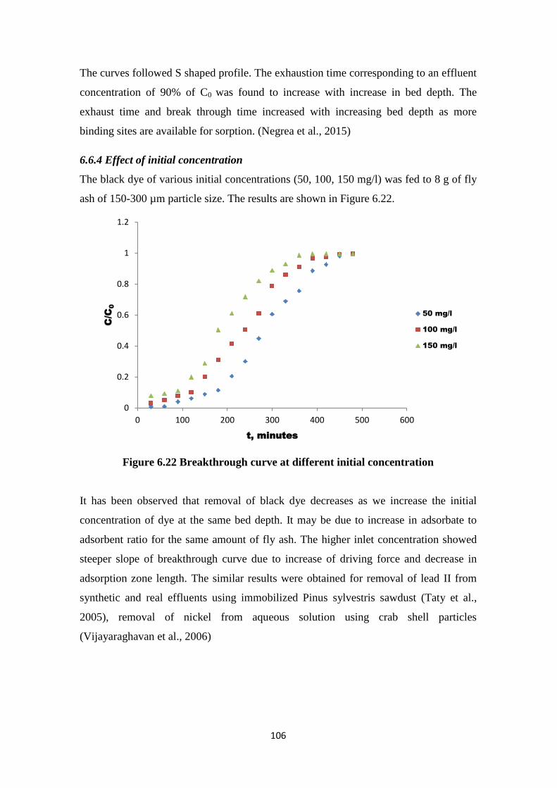
106
The curves followed S shaped profile. The exhaustion time corresponding to an effluent
concentration of 90% of C0 was found to increase with increase in bed depth. The
exhaust time and break through time increased with increasing bed depth as more
binding sites are available for sorption. (Negrea et al., 2015)
6.6.4 Effect of initial concentration
The black dye of various initial concentrations (50, 100, 150 mg/l) was fed to 8 g of fly
ash of 150-300 µm particle size. The results are shown in Figure 6.22.
Figure 6.22 Breakthrough curve at different initial concentration
It has been observed that removal of black dye decreases as we increase the initial
concentration of dye at the same bed depth. It may be due to increase in adsorbate to
adsorbent ratio for the same amount of fly ash. The higher inlet concentration showed
steeper slope of breakthrough curve due to increase of driving force and decrease in
adsorption zone length. The similar results were obtained for removal of lead II from
synthetic and real effluents using immobilized Pinus sylvestris sawdust (Taty et al.,
2005), removal of nickel from aqueous solution using crab shell particles
(Vijayaraghavan et al., 2006)
0
0.2
0.4
0.6
0.8
1
1.2
0 100 200 300 400 500 600
C/C
0
t, minutes
50 mg/l
100 mg/l
150 mg/l
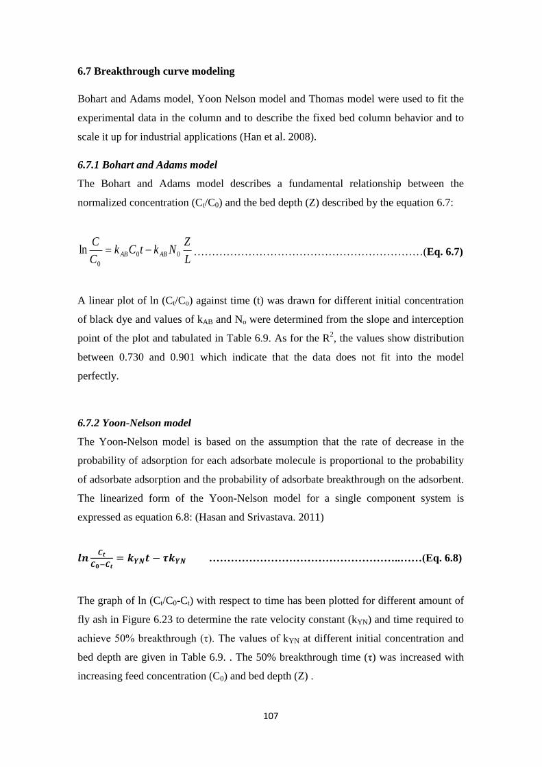
107
6.7 Breakthrough curve modeling
Bohart and Adams model, Yoon Nelson model and Thomas model were used to fit the
experimental data in the column and to describe the fixed bed column behavior and to
scale it up for industrial applications (Han et al. 2008).
6.7.1 Bohart and Adams model
The Bohart and Adams model describes a fundamental relationship between the
normalized concentration (Ct/C0) and the bed depth (Z) described by the equation 6.7:
L
ZNktCk
C
CABAB 00
0
ln ………………………………………………………(Eq. 6.7)
A linear plot of ln (Ct/Co) against time (t) was drawn for different initial concentration
of black dye and values of kAB and No were determined from the slope and interception
point of the plot and tabulated in Table 6.9. As for the R2, the values show distribution
between 0.730 and 0.901 which indicate that the data does not fit into the model
perfectly.
6.7.2 Yoon-Nelson model
The Yoon-Nelson model is based on the assumption that the rate of decrease in the
probability of adsorption for each adsorbate molecule is proportional to the probability
of adsorbate adsorption and the probability of adsorbate breakthrough on the adsorbent.
The linearized form of the Yoon-Nelson model for a single component system is
expressed as equation 6.8: (Hasan and Srivastava. 2011)
𝒍𝒏𝑪𝒕
𝑪𝟎−𝑪𝒕= 𝒌𝒀𝑵𝒕 − 𝝉𝒌𝒀𝑵 ……………………………………………..……(Eq. 6.8)
The graph of ln (Ct/C0-Ct) with respect to time has been plotted for different amount of
fly ash in Figure 6.23 to determine the rate velocity constant (kYN) and time required to
achieve 50% breakthrough (τ). The values of kYN at different initial concentration and
bed depth are given in Table 6.9. . The 50% breakthrough time (τ) was increased with
increasing feed concentration (C0) and bed depth (Z) .
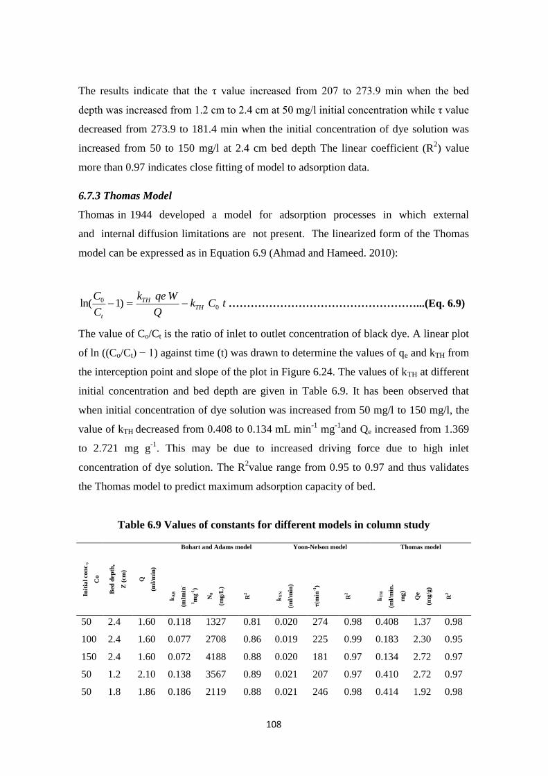
108
The results indicate that the τ value increased from 207 to 273.9 min when the bed
depth was increased from 1.2 cm to 2.4 cm at 50 mg/l initial concentration while τ value
decreased from 273.9 to 181.4 min when the initial concentration of dye solution was
increased from 50 to 150 mg/l at 2.4 cm bed depth The linear coefficient (R2) value
more than 0.97 indicates close fitting of model to adsorption data.
6.7.3 Thomas Model
Thomas in 1944 developed a model for adsorption processes in which external
and internal diffusion limitations are not present. The linearized form of the Thomas
model can be expressed as in Equation 6.9 (Ahmad and Hameed. 2010):
tCkQ
Wqek
C
CTH
TH
t
00 )1ln( ……………………………………………...(Eq. 6.9)
The value of Co/Ct is the ratio of inlet to outlet concentration of black dye. A linear plot
of ln ((Co/Ct) − 1) against time (t) was drawn to determine the values of qe and kTH from
the interception point and slope of the plot in Figure 6.24. The values of kTH at different
initial concentration and bed depth are given in Table 6.9. It has been observed that
when initial concentration of dye solution was increased from 50 mg/l to 150 mg/l, the
value of kTH decreased from 0.408 to 0.134 mL min-1
mg-1
and Qe increased from 1.369
to 2.721 mg g-1
. This may be due to increased driving force due to high inlet
concentration of dye solution. The R2value range from 0.95 to 0.97 and thus validates
the Thomas model to predict maximum adsorption capacity of bed.
Table 6.9 Values of constants for different models in column study
Init
ial
con
c.,
Co
Bed
dep
th,
Z (
cm
)
Q
(ml/
min
)
Bohart and Adams model Yoon-Nelson model Thomas model
kA
B
(mlm
in-
1m
g-1
)
N0
(mg/L
)
R2
kY
N
(ml/
min
)
τ(m
in-1
)
R2
kT
H
(ml/
min
.
mg)
Qe
(mg/g
)
R2
50 2.4 1.60 0.118 1327 0.81 0.020 274 0.98 0.408 1.37 0.98
100 2.4 1.60 0.077 2708 0.86 0.019 225 0.99 0.183 2.30 0.95
150 2.4 1.60 0.072 4188 0.88 0.020 181 0.97 0.134 2.72 0.97
50 1.2 2.10 0.138 3567 0.89 0.021 207 0.97 0.410 2.72 0.97
50 1.8 1.86 0.186 2119 0.88 0.021 246 0.98 0.414 1.92 0.98
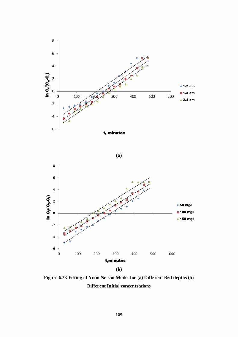
109
(a)
(b)
Figure 6.23 Fitting of Yoon Nelson Model for (a) Different Bed depths (b)
Different Initial concentrations
-6
-4
-2
0
2
4
6
8
0 100 200 300 400 500 600ln C
t/(C
0-C
t)
t, minutes
1.2 cm
1.8 cm
2.4 cm
-6
-4
-2
0
2
4
6
8
0 100 200 300 400 500 600
ln C
t/(C
0-C
t)
t,minutes
50 mg/l
100 mg/l
150 mg/l
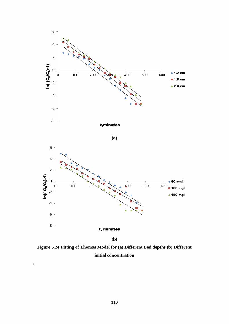
110
(a)
(b)
Figure 6.24 Fitting of Thomas Model for (a) Different Bed depths (b) Different
initial concentration
,
-8
-6
-4
-2
0
2
4
6
0 100 200 300 400 500 600
ln( (C
0/C
t)-1)
t,minutes
1.2 cm
1.8 cm
2.4 cm
-8
-6
-4
-2
0
2
4
6
0 100 200 300 400 500 600
ln(( C
0/C
t)-1)
t, minutes
50 mg/l
100 mg/l
150 mg/l
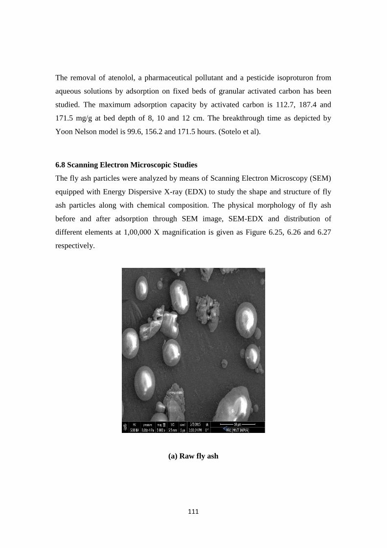
111
The removal of atenolol, a pharmaceutical pollutant and a pesticide isoproturon from
aqueous solutions by adsorption on fixed beds of granular activated carbon has been
studied. The maximum adsorption capacity by activated carbon is 112.7, 187.4 and
171.5 mg/g at bed depth of 8, 10 and 12 cm. The breakthrough time as depicted by
Yoon Nelson model is 99.6, 156.2 and 171.5 hours. (Sotelo et al).
6.8 Scanning Electron Microscopic Studies
The fly ash particles were analyzed by means of Scanning Electron Microscopy (SEM)
equipped with Energy Dispersive X-ray (EDX) to study the shape and structure of fly
ash particles along with chemical composition. The physical morphology of fly ash
before and after adsorption through SEM image, SEM-EDX and distribution of
different elements at 1,00,000 X magnification is given as Figure 6.25, 6.26 and 6.27
respectively.
(a) Raw fly ash
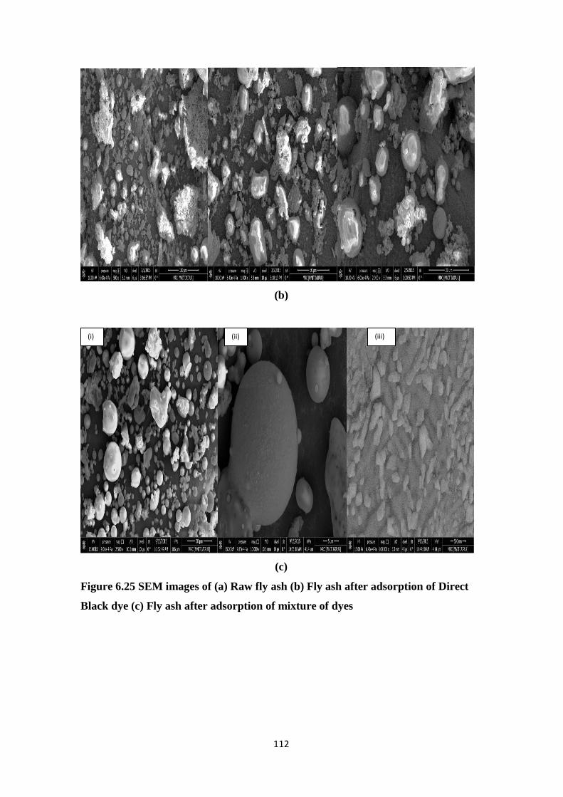
112
(b)
(c)
Figure 6.25 SEM images of (a) Raw fly ash (b) Fly ash after adsorption of Direct
Black dye (c) Fly ash after adsorption of mixture of dyes
(i) (ii) (iii)
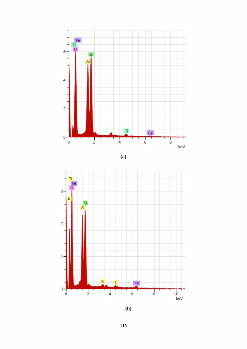
113
(a)
(b)
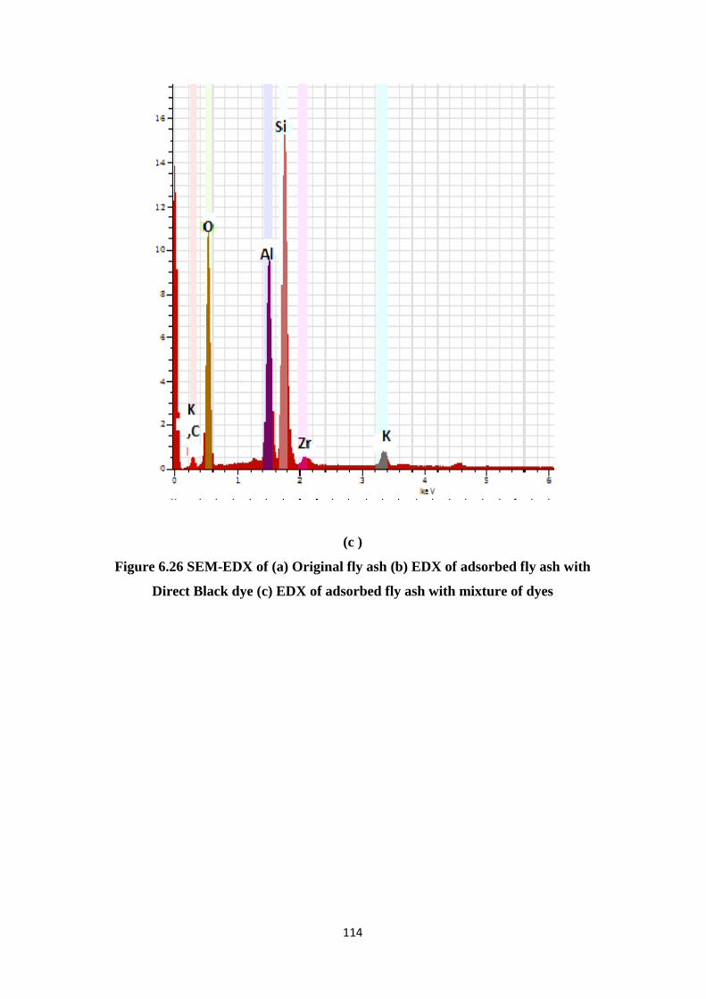
114
(c )
Figure 6.26 SEM-EDX of (a) Original fly ash (b) EDX of adsorbed fly ash with
Direct Black dye (c) EDX of adsorbed fly ash with mixture of dyes
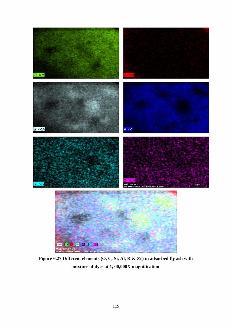
115
Figure 6.27 Different elements (O, C, Si, Al, K & Zr) in adsorbed fly ash with
mixture of dyes at 1, 00,000X magnification
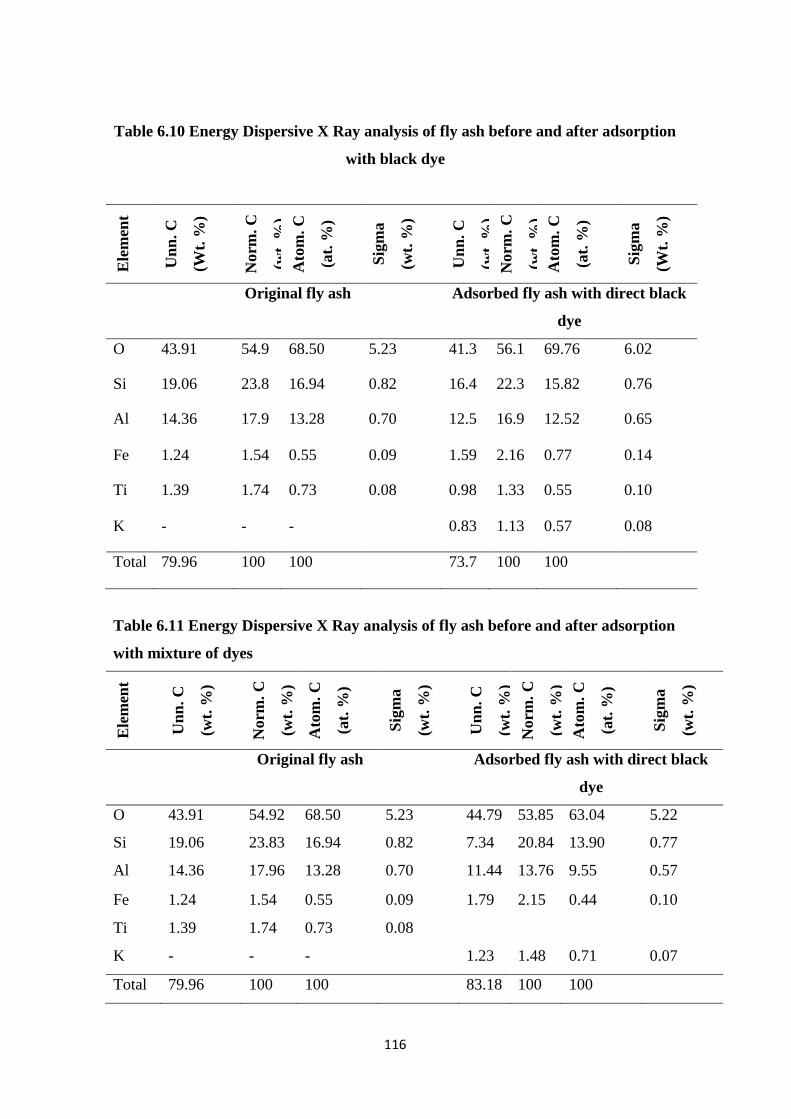
116
Table 6.10 Energy Dispersive X Ray analysis of fly ash before and after adsorption
with black dye
Ele
men
t
Un
n. C
(Wt.
%)
Norm
. C
(wt.
%)
Ato
m. C
(at.
%)
Sig
ma
(wt.
%)
Un
n. C
(wt.
%)
Norm
. C
(wt.
%)
Ato
m. C
(at.
%)
Sig
ma
(Wt.
%)
Original fly ash Adsorbed fly ash with direct black
dye
O 43.91 54.9 68.50 5.23 41.3 56.1 69.76 6.02
Si 19.06 23.8 16.94 0.82 16.4 22.3 15.82 0.76
Al 14.36 17.9 13.28 0.70 12.5 16.9 12.52 0.65
Fe 1.24 1.54 0.55 0.09 1.59 2.16 0.77 0.14
Ti 1.39 1.74 0.73 0.08 0.98 1.33 0.55 0.10
K - - - 0.83 1.13 0.57 0.08
Total 79.96 100 100 73.7 100 100
Table 6.11 Energy Dispersive X Ray analysis of fly ash before and after adsorption
with mixture of dyes
Ele
men
t
Un
n. C
(wt.
%)
Norm
. C
(wt.
%)
Ato
m. C
(at.
%)
Sig
ma
(wt.
%)
Un
n. C
(wt.
%)
Norm
. C
(wt.
%)
Ato
m. C
(at.
%)
Sig
ma
(wt.
%)
Original fly ash Adsorbed fly ash with direct black
dye
O 43.91 54.92 68.50 5.23 44.79 53.85 63.04 5.22
Si 19.06 23.83 16.94 0.82 7.34 20.84 13.90 0.77
Al 14.36 17.96 13.28 0.70 11.44 13.76 9.55 0.57
Fe 1.24 1.54 0.55 0.09 1.79 2.15 0.44 0.10
Ti 1.39 1.74 0.73 0.08
K - - - 1.23 1.48 0.71 0.07
Total 79.96 100 100 83.18 100 100
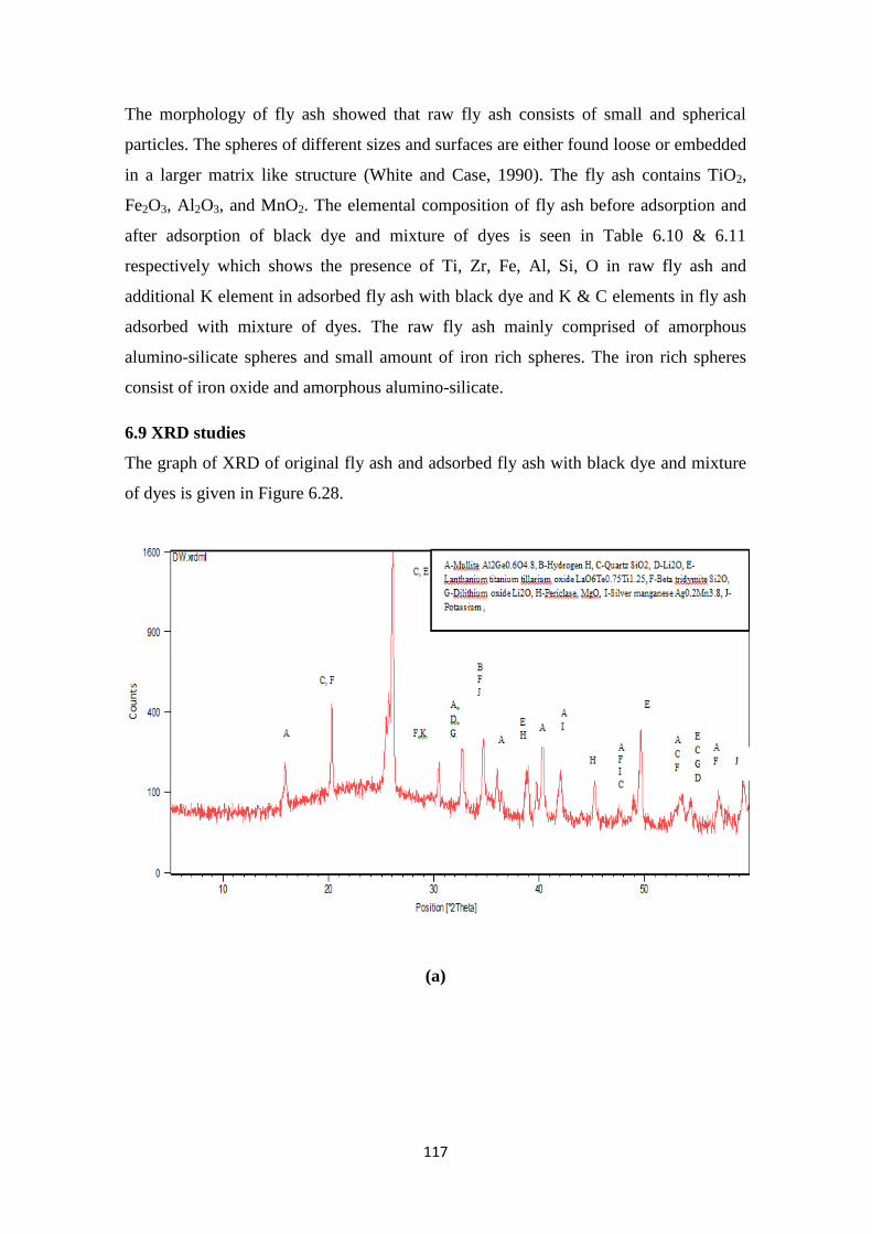
117
The morphology of fly ash showed that raw fly ash consists of small and spherical
particles. The spheres of different sizes and surfaces are either found loose or embedded
in a larger matrix like structure (White and Case, 1990). The fly ash contains TiO2,
Fe2O3, Al2O3, and MnO2. The elemental composition of fly ash before adsorption and
after adsorption of black dye and mixture of dyes is seen in Table 6.10 & 6.11
respectively which shows the presence of Ti, Zr, Fe, Al, Si, O in raw fly ash and
additional K element in adsorbed fly ash with black dye and K & C elements in fly ash
adsorbed with mixture of dyes. The raw fly ash mainly comprised of amorphous
alumino-silicate spheres and small amount of iron rich spheres. The iron rich spheres
consist of iron oxide and amorphous alumino-silicate.
6.9 XRD studies
The graph of XRD of original fly ash and adsorbed fly ash with black dye and mixture
of dyes is given in Figure 6.28.
(a)
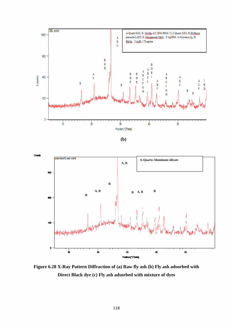
118
(b)
Figure 6.28 X-Ray Pattern Diffraction of (a) Raw fly ash (b) Fly ash adsorbed with
Direct Black dye (c) Fly ash adsorbed with mixture of dyes
A, B
A, B
B B A, B B
B
A-Quartz-Aluminum silicate
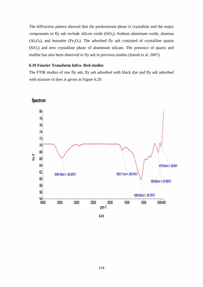
119
The diffraction pattern showed that the predominant phase is crystalline and the major
components in fly ash include silicon oxide (SiO2), Sodium aluminum oxide, alumina
(Al2O3), and hematite (Fe2O3). The adsorbed fly ash consisted of crystalline quartz
(SiO2) and new crystalline phase of aluminum silicate. The presence of quartz and
mullite has also been observed in fly ash in previous studies (Ismail et al. 2007).
6.10 Fourier Transform Infra- Red studies
The FTIR studies of raw fly ash, fly ash adsorbed with black dye and fly ash adsorbed
with mixture of dyes is given as Figure 6.29.
(a)
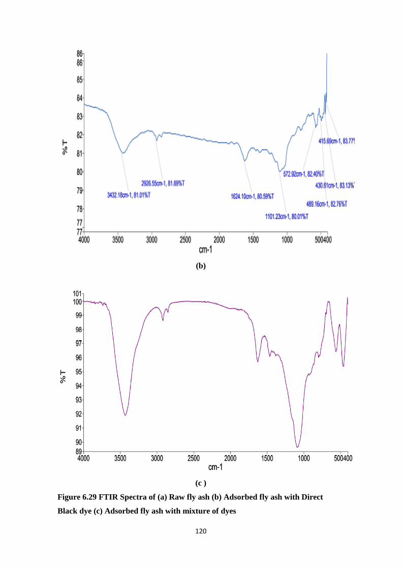
120
(b)
(c )
Figure 6.29 FTIR Spectra of (a) Raw fly ash (b) Adsorbed fly ash with Direct
Black dye (c) Adsorbed fly ash with mixture of dyes
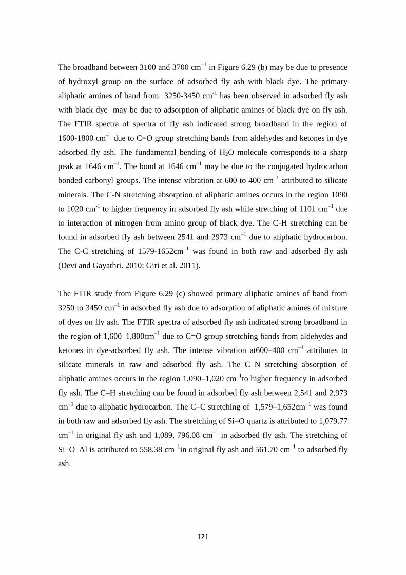
121
The broadband between 3100 and 3700 cm–1
in Figure 6.29 (b) may be due to presence
of hydroxyl group on the surface of adsorbed fly ash with black dye. The primary
aliphatic amines of band from 3250-3450 cm-1
has been observed in adsorbed fly ash
with black dye may be due to adsorption of aliphatic amines of black dye on fly ash.
The FTIR spectra of spectra of fly ash indicated strong broadband in the region of
1600-1800 cm–1
due to C=O group stretching bands from aldehydes and ketones in dye
adsorbed fly ash. The fundamental bending of H2O molecule corresponds to a sharp
peak at 1646 cm–1
. The bond at 1646 cm–1
may be due to the conjugated hydrocarbon
bonded carbonyl groups. The intense vibration at 600 to 400 cm–1
attributed to silicate
minerals. The C-N stretching absorption of aliphatic amines occurs in the region 1090
to 1020 cm-1
to higher frequency in adsorbed fly ash while stretching of 1101 cm–1
due
to interaction of nitrogen from amino group of black dye. The C-H stretching can be
found in adsorbed fly ash between 2541 and 2973 cm–1
due to aliphatic hydrocarbon.
The C-C stretching of 1579-1652cm–1
was found in both raw and adsorbed fly ash
(Devi and Gayathri. 2010; Giri et al. 2011).
The FTIR study from Figure 6.29 (c) showed primary aliphatic amines of band from
3250 to 3450 cm–1
in adsorbed fly ash due to adsorption of aliphatic amines of mixture
of dyes on fly ash. The FTIR spectra of adsorbed fly ash indicated strong broadband in
the region of 1,600–1,800cm–1
due to C=O group stretching bands from aldehydes and
ketones in dye-adsorbed fly ash. The intense vibration at600–400 cm–1
attributes to
silicate minerals in raw and adsorbed fly ash. The C–N stretching absorption of
aliphatic amines occurs in the region 1,090–1,020 cm–1
to higher frequency in adsorbed
fly ash. The C–H stretching can be found in adsorbed fly ash between 2,541 and 2,973
cm–1
due to aliphatic hydrocarbon. The C–C stretching of 1,579–1,652cm–1
was found
in both raw and adsorbed fly ash. The stretching of Si–O quartz is attributed to 1,079.77
cm–1
in original fly ash and 1,089, 796.08 cm–1
in adsorbed fly ash. The stretching of
Si–O–Al is attributed to 558.38 cm–1
in original fly ash and 561.70 cm–1
to adsorbed fly
ash.
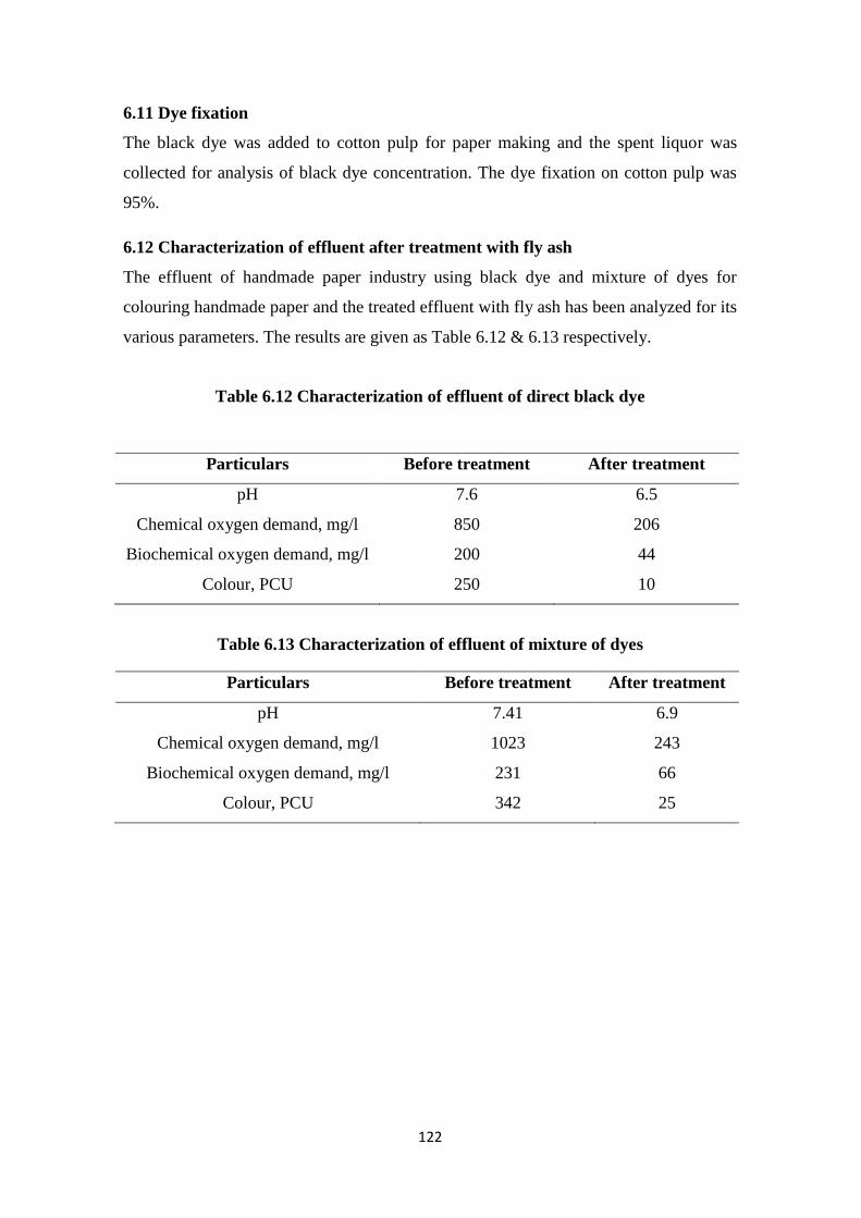
122
6.11 Dye fixation
The black dye was added to cotton pulp for paper making and the spent liquor was
collected for analysis of black dye concentration. The dye fixation on cotton pulp was
95%.
6.12 Characterization of effluent after treatment with fly ash
The effluent of handmade paper industry using black dye and mixture of dyes for
colouring handmade paper and the treated effluent with fly ash has been analyzed for its
various parameters. The results are given as Table 6.12 & 6.13 respectively.
Table 6.12 Characterization of effluent of direct black dye
Particulars Before treatment After treatment
pH 7.6 6.5
Chemical oxygen demand, mg/l 850 206
Biochemical oxygen demand, mg/l 200 44
Colour, PCU 250 10
Table 6.13 Characterization of effluent of mixture of dyes
Particulars Before treatment After treatment
pH 7.41 6.9
Chemical oxygen demand, mg/l 1023 243
Biochemical oxygen demand, mg/l 231 66
Colour, PCU 342 25
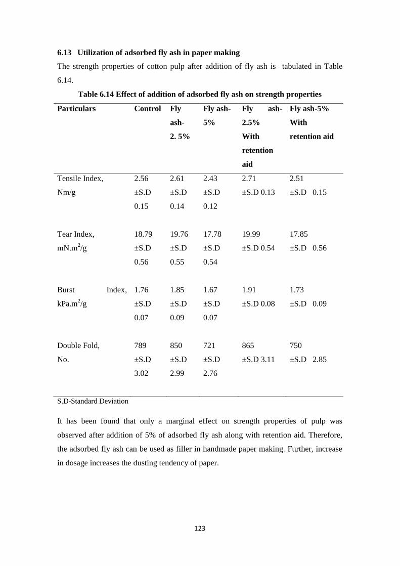
123
6.13 Utilization of adsorbed fly ash in paper making
The strength properties of cotton pulp after addition of fly ash is tabulated in Table
6.14.
Table 6.14 Effect of addition of adsorbed fly ash on strength properties
Particulars Control Fly
ash-
2. 5%
Fly ash-
5%
Fly ash-
2.5%
With
retention
aid
Fly ash-5%
With
retention aid
Tensile Index,
Nm/g
2.56
±S.D
0.15
2.61
±S.D
0.14
2.43
±S.D
0.12
2.71
±S.D 0.13
2.51
±S.D 0.15
Tear Index,
mN.m2/g
18.79
±S.D
0.56
19.76
±S.D
0.55
17.78
±S.D
0.54
19.99
±S.D 0.54
17.85
±S.D 0.56
Burst Index,
kPa.m2/g
1.76
±S.D
0.07
1.85
±S.D
0.09
1.67
±S.D
0.07
1.91
±S.D 0.08
1.73
±S.D 0.09
Double Fold,
No.
789
±S.D
3.02
850
±S.D
2.99
721
±S.D
2.76
865
±S.D 3.11
750
±S.D 2.85
S.D-Standard Deviation
It has been found that only a marginal effect on strength properties of pulp was
observed after addition of 5% of adsorbed fly ash along with retention aid. Therefore,
the adsorbed fly ash can be used as filler in handmade paper making. Further, increase
in dosage increases the dusting tendency of paper.
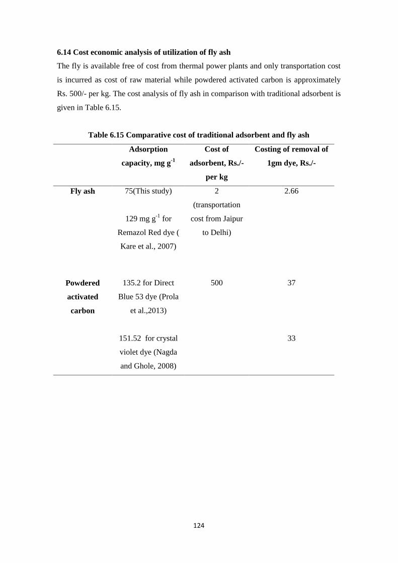
124
6.14 Cost economic analysis of utilization of fly ash
The fly is available free of cost from thermal power plants and only transportation cost
is incurred as cost of raw material while powdered activated carbon is approximately
Rs. 500/- per kg. The cost analysis of fly ash in comparison with traditional adsorbent is
given in Table 6.15.
Table 6.15 Comparative cost of traditional adsorbent and fly ash
Adsorption
capacity, mg g-1
Cost of
adsorbent, Rs./-
per kg
Costing of removal of
1gm dye, Rs./-
Fly ash 75(This study)
129 mg g-1
for
Remazol Red dye (
Kare et al., 2007)
2
(transportation
cost from Jaipur
to Delhi)
2.66
Powdered
activated
carbon
135.2 for Direct
Blue 53 dye (Prola
et al.,2013)
151.52 for crystal
violet dye (Nagda
and Ghole, 2008)
500 37
33
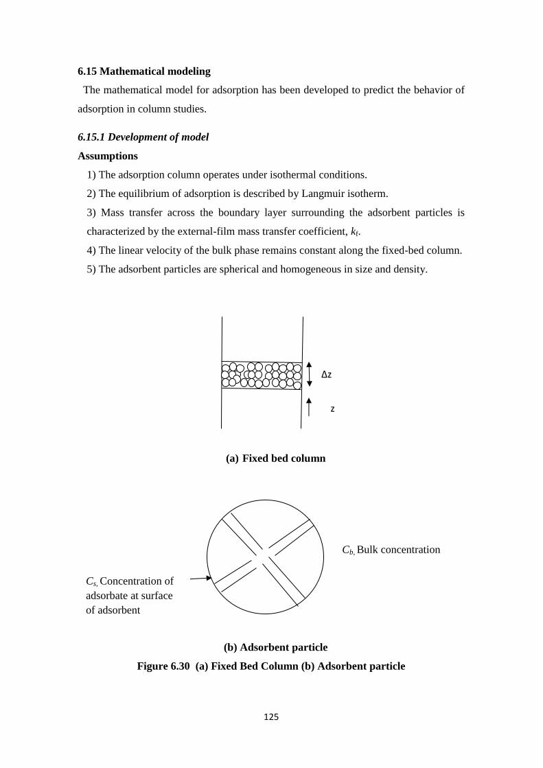
125
6.15 Mathematical modeling
The mathematical model for adsorption has been developed to predict the behavior of
adsorption in column studies.
6.15.1 Development of model
Assumptions
1) The adsorption column operates under isothermal conditions.
2) The equilibrium of adsorption is described by Langmuir isotherm.
3) Mass transfer across the boundary layer surrounding the adsorbent particles is
characterized by the external-film mass transfer coefficient, kf.
4) The linear velocity of the bulk phase remains constant along the fixed-bed column.
5) The adsorbent particles are spherical and homogeneous in size and density.
(a) Fixed bed column
(b) Adsorbent particle
Figure 6.30 (a) Fixed Bed Column (b) Adsorbent particle
∆z
z
Cb, Bulk concentration
B Cs, Concentration of
adsorbate at surface
of adsorbent
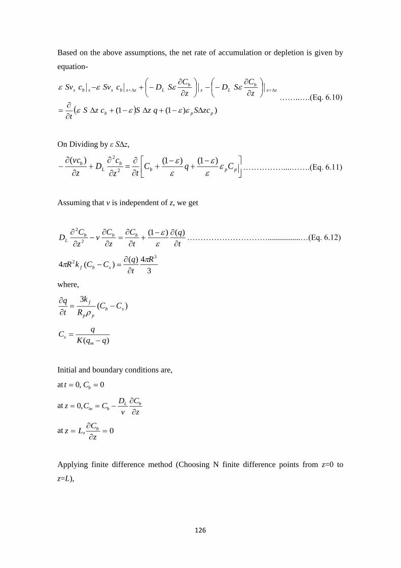
126
Based on the above assumptions, the net rate of accumulation or depletion is given by
equation-
))1(1( ppb
zz
b
Lz
b
Lzzbszbs
zcSqzSczSt
z
CSD
z
CSDcSvcSv
……..….(Eq. 6.10)
On Dividing by ε S∆z,
ppb
b
L
b CqCtz
cD
z
vc
)1()1()(2
2
……………....…….(Eq. 6.11)
Assuming that v is independent of z, we get
t
q
t
C
z
Cv
z
CD bbb
L
)()1(2
2
…………………………................…(Eq. 6.12)
3
4)()(4
32 R
t
qCCkR sbf
where,
)(3
sb
pp
fCC
R
k
t
q
)( qqK
qC
m
s
Initial and boundary conditions are,
at 0,0 bCt
atz
C
v
DCCz bL
bin
,0
at 0,
z
CLz b
Applying finite difference method (Choosing N finite difference points from z=0 to
z=L),
127
At z=0,
)2
( 02
1z
CC
v
DCC bbL
bin
…………………….……………………….…….(Eq. 6.13)
or,
2
1
0
2)(b
L
bin
b CD
zvCCC
………………………………………….……….(Eq. 6.14)
At i=1
L
inb
b
D
vCC
z
C)( 1
…………………………………………………..…….(Eq. 6.15)
or, L
inb
bb
D
vCC
z
CC)(
21
02
…………………………………..……………(Eq. 6.16)
or, L
binb
bbD
CCvzCC
)(2 1
20
……………………………………………..(Eq. 6.17)
Second order derivative becomes,
2
012
2
2 2
z
CCC
z
C bbbb
……………………………………………………..(Eq. 6.18)
Therefore,
…..………………………(Eq. 6.19)
or, 2
1212
2
2
222
z
CD
vzC
D
vzCCC
z
Cbin
L
b
L
bbb
b
……………………….(Eq. 6.20)
or,
2
12
2
2
2)1(22
z
CD
vz
D
vzCC
z
Cbin
LL
bb
b
……………………...…………..(Eq. 6.21)
2
1
212
2
2)
)(2(2
z
D
CCvzCCC
z
C L
binbbbb
b
128
At i=N
22
2
112
z
CCC
z
CNNN bbbb
………………………………………..…………(Eq. 6.22)
0)(2
,0 11
z
CC
z
CN
bNbb…………………...……………………………(Eq. 6.23)
or,
11
NNbb CC
Therefore,
22
2 )2(21
z
CC
z
CNN bbb
…………………………………….…………………(Eq. 6.24)
6.15.2 Determination of external mass transfer coefficient
According to McKay plot of kinetic curves (Yesim Sag et al 2000), the equation of
determination of external mass transfer coefficient is given by:
tSk
mK
mK
mK
mK
mKC
Csf
1
1ln
1
1ln
0
…………….....……….…..(Eq. 6.25)
Where,
)1(
6
ppp
sd
mS
6.15.3 Determination of axial dispersion coefficient
As per Ruthven (1984), the equation of determination of axial dispersion coefficient is
given by
2
120
00
p
m
p
L
du
D
du
D
…………………………………………………….. (Eq. 6.26)
Where,
u0= superficial velocity, m/s
dp=particle diameter, m
Dm=molecular diffusivity of dye in water, m2/s
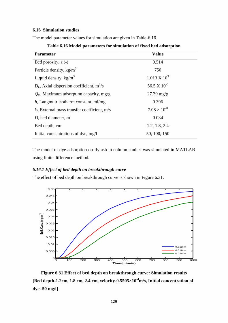
129
6.16 Simulation studies
The model parameter values for simulation are given in Table-6.16.
Table 6.16 Model parameters for simulation of fixed bed adsorption
Parameter Value
Bed porosity, ε (-) 0.514
Particle density, kg/m3 750
Liquid density, kg/m3 1.013 X 10
3
DL, Axial dispersion coefficient, m2/s 56.5 X 10
-5
Qm, Maximum adsorption capacity, mg/g 27.39 mg/g
b, Langmuir isotherm constant, ml/mg 0.396
kf, External mass transfer coefficient, m/s 7.08 × 10⁻⁸
D, bed diameter, m 0.034
Bed depth, cm 1.2, 1.8, 2.4
Initial concentrations of dye, mg/l 50, 100, 150
The model of dye adsorption on fly ash in column studies was simulated in MATLAB
using finite difference method.
6.16.1 Effect of bed depth on breakthrough curve
The effect of bed depth on breakthrough curve is shown in Figure 6.31.
Figure 6.31 Effect of bed depth on breakthrough curve: Simulation results
[Bed depth-1.2cm, 1.8 cm, 2.4 cm, velocity-0.5505×10⁻⁴
m/s, Initial concentration of
dye=50 mg/l]
0 100 200 300 400 500 600 700 800 900 10000
0.005
0.01
0.015
0.02
0.025
0.03
0.035
0.04
0.045
0.05
Time(minute)
Bulk
Con
c. (m
g/m
3 )
0.012 m
0.018 m
0.024 m
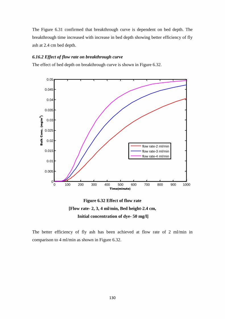
130
The Figure 6.31 confirmed that breakthrough curve is dependent on bed depth. The
breakthrough time increased with increase in bed depth showing better efficiency of fly
ash at 2.4 cm bed depth.
6.16.2 Effect of flow rate on breakthrough curve
The effect of bed depth on breakthrough curve is shown in Figure 6.32.
Figure 6.32 Effect of flow rate
[Flow rate- 2, 3, 4 ml/min, Bed height-2.4 cm,
Initial concentration of dye- 50 mg/l]
The better efficiency of fly ash has been achieved at flow rate of 2 ml/min in
comparison to 4 ml/min as shown in Figure 6.32.
0 100 200 300 400 500 600 700 800 900 10000
0.005
0.01
0.015
0.02
0.025
0.03
0.035
0.04
0.045
0.05
Time(minute)
Bulk C
onc. (m
g/m
3
)
flow rate-2 ml/min
flow rate-3 ml/min
flow rate-4 ml/min
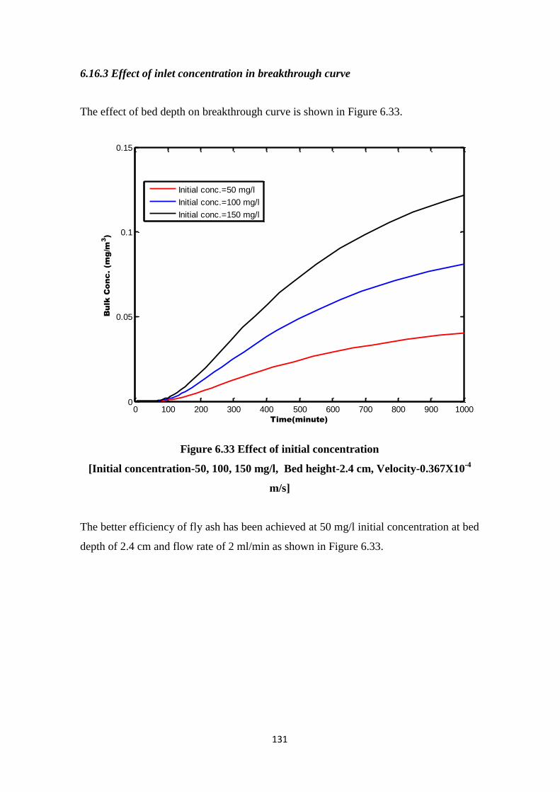
131
6.16.3 Effect of inlet concentration in breakthrough curve
The effect of bed depth on breakthrough curve is shown in Figure 6.33.
Figure 6.33 Effect of initial concentration
[Initial concentration-50, 100, 150 mg/l, Bed height-2.4 cm, Velocity-0.367X10⁻⁴
m/s]
The better efficiency of fly ash has been achieved at 50 mg/l initial concentration at bed
depth of 2.4 cm and flow rate of 2 ml/min as shown in Figure 6.33.
0 100 200 300 400 500 600 700 800 900 10000
0.05
0.1
0.15
Time(minute)
Bu
lk C
onc
. (m
g/m
3
)
Initial conc.=50 mg/l
Initial conc.=100 mg/l
Initial conc.=150 mg/l
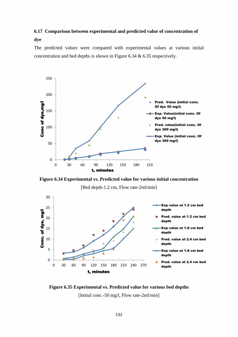
132
6.17 Comparison between experimental and predicted value of concentration of
dye
The predicted values were compared with experimental values at various initial
concentration and bed depths is shown in Figure 6.34 & 6.35 respectively.
Figure 6.34 Experimental vs. Predicted value for various initial concentration
[Bed depth-1.2 cm, Flow rate-2ml/min]
Figure 6.35 Experimental vs. Predicted value for various bed depths
[Initial conc.-50 mg/l, Flow rate-2ml/min]
0
50
100
150
200
250
0 30 60 90 120 150 180 210
Conc of dye,m
g/l
t, minutes
Pred. Value (initial conc.
Of dye 50 mg/l)
Exp. Value(initial conc. Of
dye 50 mg/l)
Pred. value(initial conc. Of
dye 300 mg/l)
Exp. Value (initial conc. Of
dye 300 mg/l)
0
5
10
15
20
25
30
0 30 60 90 120 150 180 210 240 270
Conc. of dye, m
g/l
t, minutes
Exp value at 1.2 cm bed
depth
Pred. value at 1.2 cm bed
depth
Exp value at 1.8 cm bed
depth
Pred. value at 2.4 cm bed
depth
Exp value at 1.8 cm bed
depth
Pred. value at 2.4 cm bed
depth
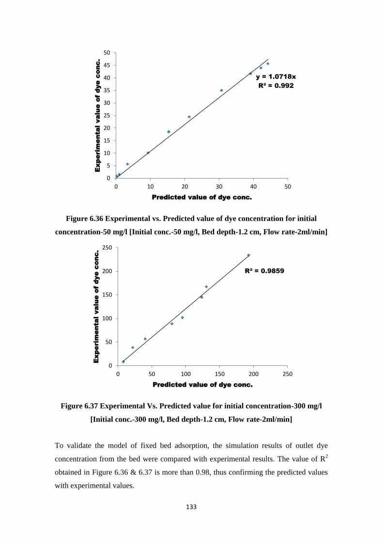
133
Figure 6.36 Experimental vs. Predicted value of dye concentration for initial
concentration-50 mg/l [Initial conc.-50 mg/l, Bed depth-1.2 cm, Flow rate-2ml/min]
Figure 6.37 Experimental Vs. Predicted value for initial concentration-300 mg/l
[Initial conc.-300 mg/l, Bed depth-1.2 cm, Flow rate-2ml/min]
To validate the model of fixed bed adsorption, the simulation results of outlet dye
concentration from the bed were compared with experimental results. The value of R2
obtained in Figure 6.36 & 6.37 is more than 0.98, thus confirming the predicted values
with experimental values.
y = 1.0718x
R² = 0.992
0
5
10
15
20
25
30
35
40
45
50
0 10 20 30 40 50
Experim
enta
l value of dye conc.
Predicted value of dye conc.
R² = 0.9859
0
50
100
150
200
250
0 50 100 150 200 250
Experim
enta
l value of dye conc.
Predicted value of dye conc.
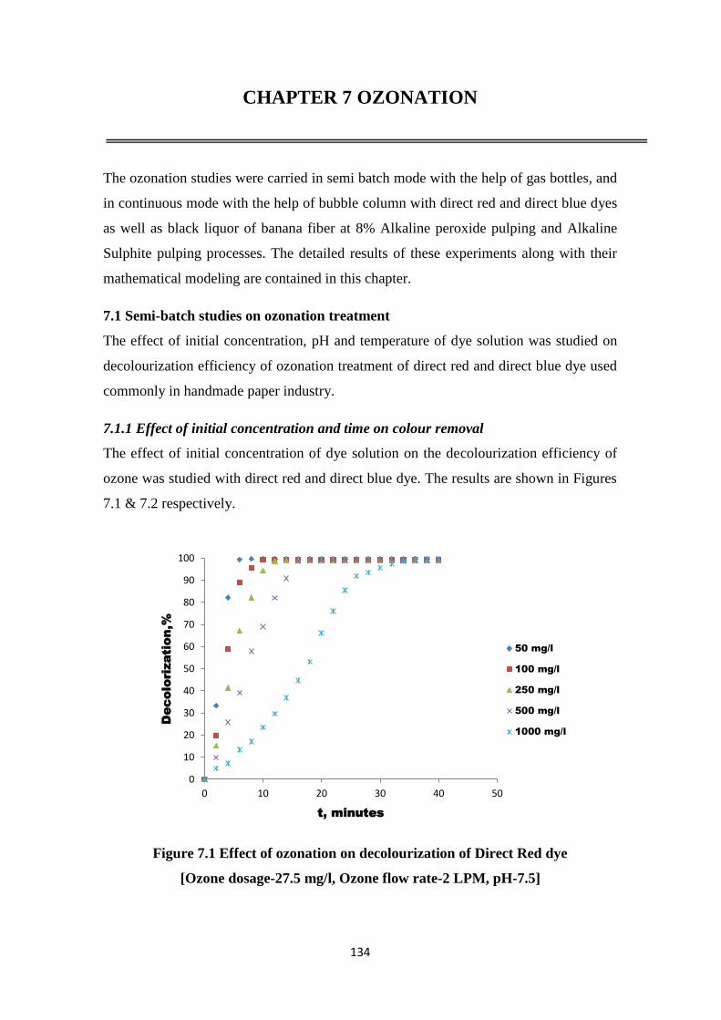
134
CHAPTER 7 OZONATION
The ozonation studies were carried in semi batch mode with the help of gas bottles, and
in continuous mode with the help of bubble column with direct red and direct blue dyes
as well as black liquor of banana fiber at 8% Alkaline peroxide pulping and Alkaline
Sulphite pulping processes. The detailed results of these experiments along with their
mathematical modeling are contained in this chapter.
7.1 Semi-batch studies on ozonation treatment
The effect of initial concentration, pH and temperature of dye solution was studied on
decolourization efficiency of ozonation treatment of direct red and direct blue dye used
commonly in handmade paper industry.
7.1.1 Effect of initial concentration and time on colour removal
The effect of initial concentration of dye solution on the decolourization efficiency of
ozone was studied with direct red and direct blue dye. The results are shown in Figures
7.1 & 7.2 respectively.
Figure 7.1 Effect of ozonation on decolourization of Direct Red dye
[Ozone dosage-27.5 mg/l, Ozone flow rate-2 LPM, pH-7.5]
0
10
20
30
40
50
60
70
80
90
100
0 10 20 30 40 50
Decolorization,%
t, minutes
50 mg/l
100 mg/l
250 mg/l
500 mg/l
1000 mg/l
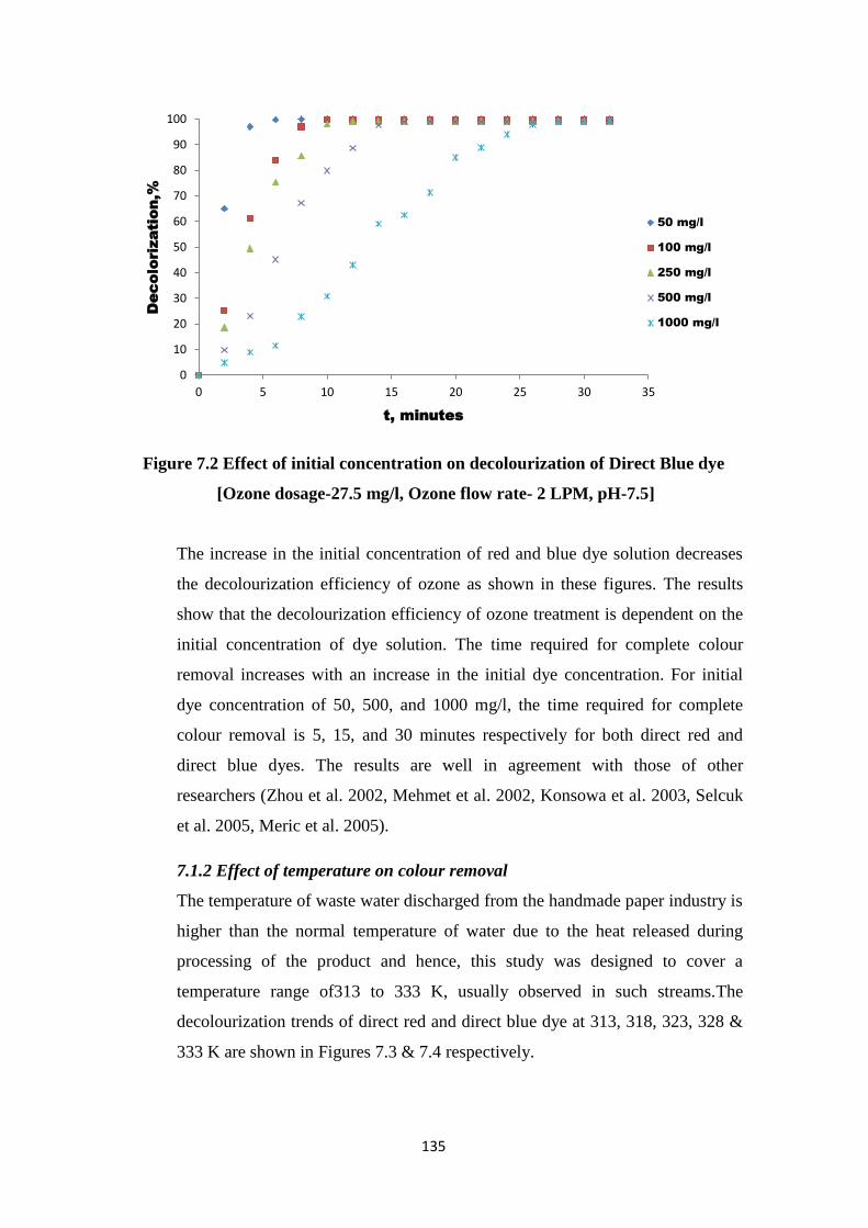
135
Figure 7.2 Effect of initial concentration on decolourization of Direct Blue dye
[Ozone dosage-27.5 mg/l, Ozone flow rate- 2 LPM, pH-7.5]
The increase in the initial concentration of red and blue dye solution decreases
the decolourization efficiency of ozone as shown in these figures. The results
show that the decolourization efficiency of ozone treatment is dependent on the
initial concentration of dye solution. The time required for complete colour
removal increases with an increase in the initial dye concentration. For initial
dye concentration of 50, 500, and 1000 mg/l, the time required for complete
colour removal is 5, 15, and 30 minutes respectively for both direct red and
direct blue dyes. The results are well in agreement with those of other
researchers (Zhou et al. 2002, Mehmet et al. 2002, Konsowa et al. 2003, Selcuk
et al. 2005, Meric et al. 2005).
7.1.2 Effect of temperature on colour removal
The temperature of waste water discharged from the handmade paper industry is
higher than the normal temperature of water due to the heat released during
processing of the product and hence, this study was designed to cover a
temperature range of313 to 333 K, usually observed in such streams.The
decolourization trends of direct red and direct blue dye at 313, 318, 323, 328 &
333 K are shown in Figures 7.3 & 7.4 respectively.
0
10
20
30
40
50
60
70
80
90
100
0 5 10 15 20 25 30 35
Decolorization,%
t, minutes
50 mg/l
100 mg/l
250 mg/l
500 mg/l
1000 mg/l

136
Figure 7.3 Effect of temperature on decolourization of Direct Red dye
[Ozone dosage-27.5 mg/l, Ozone flow rate- 2 LPM,
Initial concentration-50 mg/l, pH-7.5]
Figure 7.4 Effect of temperature on decolourization of Direct Blue dye
[Ozone dosage-27.5 mg/l, Ozone flow rate- 2 LPM,
Initial concentration-50 mg/l, pH-7.5]
0
10
20
30
40
50
60
70
80
90
100
0 2 4 6 8 10 12 14 16 18 20 22
Decolourization,%
t,minutes
313 K
318 K
323 K
328 K
333 K
0
10
20
30
40
50
60
70
80
90
100
0 5 10 15 20 25
De
co
lo
uriza
tio
n,%
t,minutes
313 K
318 K
323 K
328 K
333 K
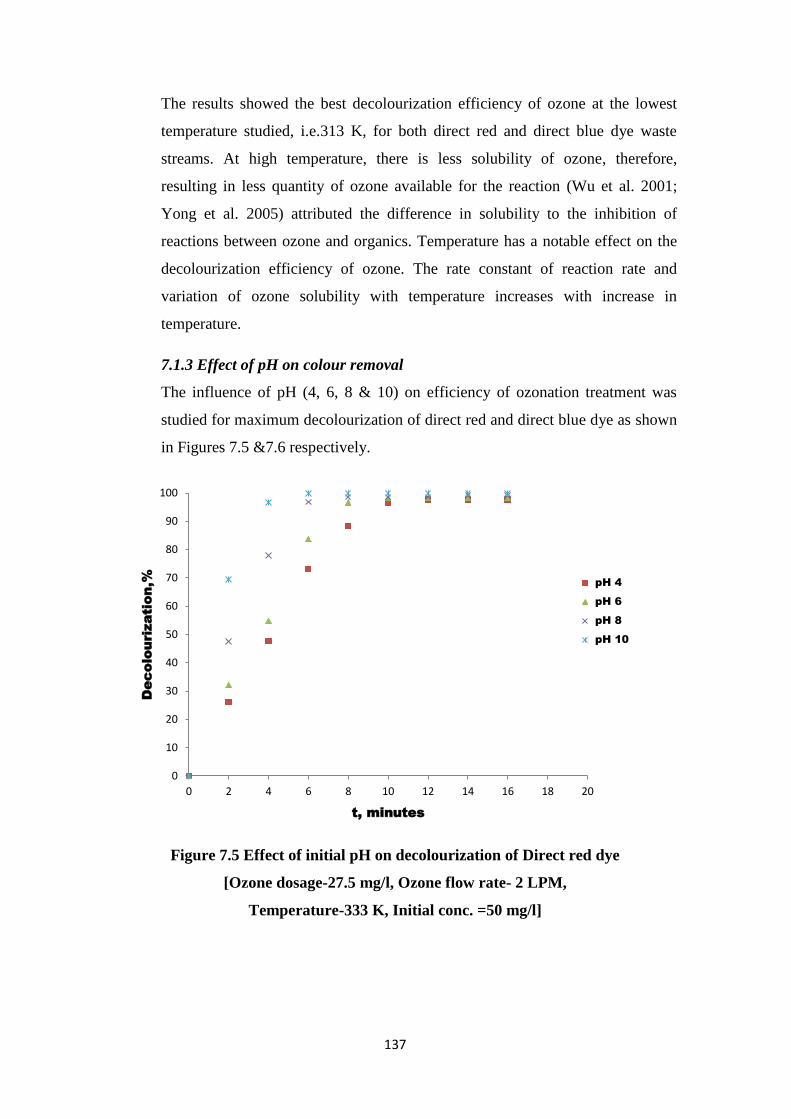
137
The results showed the best decolourization efficiency of ozone at the lowest
temperature studied, i.e.313 K, for both direct red and direct blue dye waste
streams. At high temperature, there is less solubility of ozone, therefore,
resulting in less quantity of ozone available for the reaction (Wu et al. 2001;
Yong et al. 2005) attributed the difference in solubility to the inhibition of
reactions between ozone and organics. Temperature has a notable effect on the
decolourization efficiency of ozone. The rate constant of reaction rate and
variation of ozone solubility with temperature increases with increase in
temperature.
7.1.3 Effect of pH on colour removal
The influence of pH (4, 6, 8 & 10) on efficiency of ozonation treatment was
studied for maximum decolourization of direct red and direct blue dye as shown
in Figures 7.5 &7.6 respectively.
Figure 7.5 Effect of initial pH on decolourization of Direct red dye
[Ozone dosage-27.5 mg/l, Ozone flow rate- 2 LPM,
Temperature-333 K, Initial conc. =50 mg/l]
0
10
20
30
40
50
60
70
80
90
100
0 2 4 6 8 10 12 14 16 18 20
Decolourization,%
t, minutes
pH 4
pH 6
pH 8
pH 10
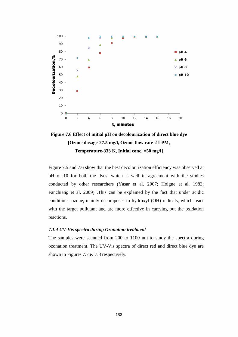
138
Figure 7.6 Effect of initial pH on decolourization of direct blue dye
[Ozone dosage-27.5 mg/l, Ozone flow rate-2 LPM,
Temperature-333 K, Initial conc. =50 mg/l]
Figure 7.5 and 7.6 show that the best decolourization efficiency was observed at
pH of 10 for both the dyes, which is well in agreement with the studies
conducted by other researchers (Yasar et al. 2007; Hoigne et al. 1983;
Fanchiang et al. 2009) .This can be explained by the fact that under acidic
conditions, ozone, mainly decomposes to hydroxyl (OH) radicals, which react
with the target pollutant and are more effective in carrying out the oxidation
reactions.
7.1.4 UV-Vis spectra during Ozonation treatment
The samples were scanned from 200 to 1100 nm to study the spectra during
ozonation treatment. The UV-Vis spectra of direct red and direct blue dye are
shown in Figures 7.7 & 7.8 respectively.
0
10
20
30
40
50
60
70
80
90
100
0 2 4 6 8 10 12 14 16 18 20
Decolourization,%
t, minutes
pH 4
pH 6
pH 8
pH 10
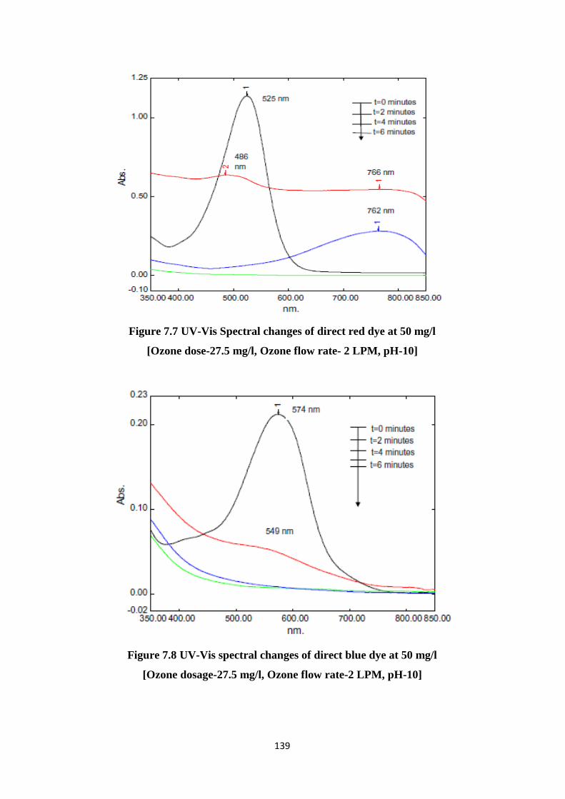
139
Figure 7.7 UV-Vis Spectral changes of direct red dye at 50 mg/l
[Ozone dose-27.5 mg/l, Ozone flow rate- 2 LPM, pH-10]
Figure 7.8 UV-Vis spectral changes of direct blue dye at 50 mg/l
[Ozone dosage-27.5 mg/l, Ozone flow rate-2 LPM, pH-10]
140
Figure 7.7 shows a bimodal development in absorbance giving one peak corresponding
to the original wavelength and another with a considerable shift at about 760 nm in
direct red dye. The reason might be the rapid destruction of dye chromophore structure
(–N=N–) by ozone. Another possibility is that this commercially available dye has two
hues with the one at 525 nm masking the other. It may be due to breaking up of original
dye in to some other molecule giving a different hue.
It has been observed from Figure 7.8 that there is no shift in wavelength corresponding
to the maximum absorbance showing that ozonation of direct blue dye solution finally
yields a colourless solution. The indicators of another peak leading to the UV range
may correspond to the intermediate organic products of ozonation reactions.
Other researchers have also reported the peak absorbance for this dye in the vicinity of
what we observed (Kozakova et al. 2010; Saroj et al. 2014) where this wavelength
should not correspond to red colour. After initial ozone reactions, the red coloured dye
is perhaps first released showing the second peak at 760 nm, and then get oxidized
further. The ozonation results well agree with those of other investigators (Paprocki et
al. 2010; Lu et al. 2009; Tehrani Bagha et al. 2010; Faria et al. 2009), but the
intermediate reaction products need to be analysed to confirm our hypothesis.
7.1.5 Kinetic studies
An attempt was made to develop an analytical model to represent the reaction kinetics
the details of which are presented below.
The reaction of ozone with solute A may be described as equation 7.1.
oxidAOA 3 ………………………………………………………………...(Eq. 7.1)
Assuming the reaction to be first order with respect to ozone and solute A which can
be formulated as equation 7.2.
][][][
3 AOkdt
AdA ……………………………………………………….…......(Eq. 7.2)
Where, kA is the rate constant for decolourization of dye solution by ozone.
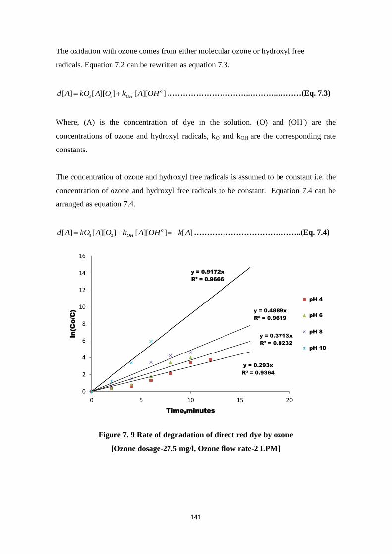
141
The oxidation with ozone comes from either molecular ozone or hydroxyl free
radicals. Equation 7.2 can be rewritten as equation 7.3.
]][[]][[][ 33
o
OH OHAkOAkOAd …………………………..………..………(Eq. 7.3)
Where, (A) is the concentration of dye in the solution. (O) and (OH-) are the
concentrations of ozone and hydroxyl radicals, kO and kOH are the corresponding rate
constants.
The concentration of ozone and hydroxyl free radicals is assumed to be constant i.e. the
concentration of ozone and hydroxyl free radicals to be constant. Equation 7.4 can be
arranged as equation 7.4.
][]][[]][[][ 33 AkOHAkOAkOAd o
OH …………………………………..(Eq. 7.4)
Figure 7. 9 Rate of degradation of direct red dye by ozone
[Ozone dosage-27.5 mg/l, Ozone flow rate-2 LPM]
y = 0.293x
R² = 0.9364
y = 0.3713x
R² = 0.9232
y = 0.4889x
R² = 0.9619
y = 0.9172x
R² = 0.9666
0
2
4
6
8
10
12
14
16
0 5 10 15 20
ln(C
o/C
)
Time,minutes
pH 4
pH 6
pH 8
pH 10
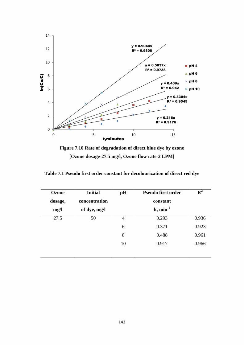
142
Figure 7.10 Rate of degradation of direct blue dye by ozone
[Ozone dosage-27.5 mg/l, Ozone flow rate-2 LPM]
Table 7.1 Pseudo first order constant for decolourization of direct red dye
Ozone
dosage,
mg/l
Initial
concentration
of dye, mg/l
pH Pseudo first order
constant
k, min-1
R2
27.5 50 4 0.293 0.936
6 0.371 0.923
8 0.488 0.961
10 0.917 0.966
y = 0.216x
R² = 0.9176
y = 0.3304x
R² = 0.9545
y = 0.409x
R² = 0.942
y = 0.5837x
R² = 0.9738
y = 0.9044x
R² = 0.9808
0
2
4
6
8
10
12
14
0 5 10 15
ln(C
o/C
)
t,minutes
pH 4
pH 6
pH 8
pH 10
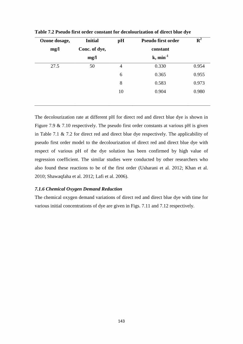
143
Table 7.2 Pseudo first order constant for decolourization of direct blue dye
Ozone dosage,
mg/l
Initial
Conc. of dye,
mg/l
pH Pseudo first order
constant
k, min-1
R2
27.5 50 4 0.330 0.954
6 0.365 0.955
8 0.583 0.973
10 0.904 0.980
The decolourization rate at different pH for direct red and direct blue dye is shown in
Figure 7.9 & 7.10 respectively. The pseudo first order constants at various pH is given
in Table 7.1 & 7.2 for direct red and direct blue dye respectively. The applicability of
pseudo first order model to the decolourization of direct red and direct blue dye with
respect of various pH of the dye solution has been confirmed by high value of
regression coefficient. The similar studies were conducted by other researchers who
also found these reactions to be of the first order (Usharani et al. 2012; Khan et al.
2010; Shawaqfaha et al. 2012; Lafi et al. 2006).
7.1.6 Chemical Oxygen Demand Reduction
The chemical oxygen demand variations of direct red and direct blue dye with time for
various initial concentrations of dye are given in Figs. 7.11 and 7.12 respectively.
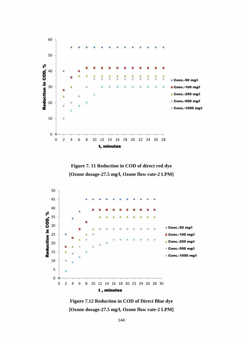
144
Figure 7. 11 Reduction in COD of direct red dye
[Ozone dosage-27.5 mg/l, Ozone flow rate-2 LPM]
Figure 7.12 Reduction in COD of Direct Blue dye
[Ozone dosage-27.5 mg/l, Ozone flow rate-2 LPM]
0
10
20
30
40
50
60
0 2 4 6 8 10 12 14 16 18 20 22 24 26 28
Reduction in C
OD
, %
t, minutes
Conc.-50 mg/l
Conc.-100 mg/l
Conc.-250 mg/l
Conc.-500 mg/l
Conc.-1000 mg/l
0
5
10
15
20
25
30
35
40
45
50
0 2 4 6 8 10 12 14 16 18 20 22 24 26 28 30
Reduction in C
OD
, %
t , minutes
Conc.-50 mg/l
Conc.-100 mg/l
Conc.-250 mg/l
Conc.-500 mg/l
Conc.-1000 mg/l
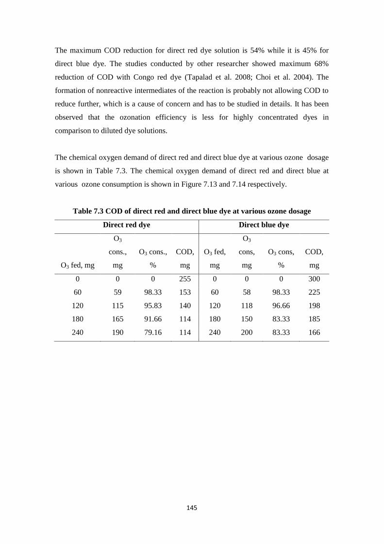
145
The maximum COD reduction for direct red dye solution is 54% while it is 45% for
direct blue dye. The studies conducted by other researcher showed maximum 68%
reduction of COD with Congo red dye (Tapalad et al. 2008; Choi et al. 2004). The
formation of nonreactive intermediates of the reaction is probably not allowing COD to
reduce further, which is a cause of concern and has to be studied in details. It has been
observed that the ozonation efficiency is less for highly concentrated dyes in
comparison to diluted dye solutions.
The chemical oxygen demand of direct red and direct blue dye at various ozone dosage
is shown in Table 7.3. The chemical oxygen demand of direct red and direct blue at
various ozone consumption is shown in Figure 7.13 and 7.14 respectively.
Table 7.3 COD of direct red and direct blue dye at various ozone dosage
Direct red dye Direct blue dye
O3 fed, mg
O3
cons.,
mg
O3 cons.,
%
COD,
mg
O3 fed,
mg
O3
cons,
mg
O3 cons,
%
COD,
mg
0 0 0 255 0 0 0 300
60 59 98.33 153 60 58 98.33 225
120 115 95.83 140 120 118 96.66 198
180 165 91.66 114 180 150 83.33 185
240 190 79.16 114 240 200 83.33 166
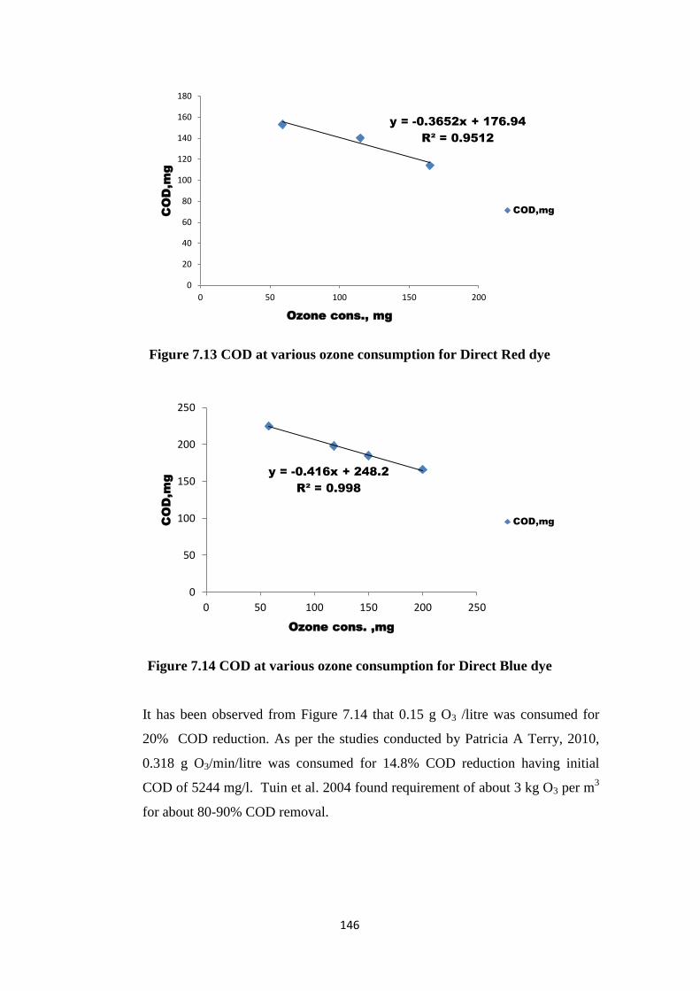
146
Figure 7.13 COD at various ozone consumption for Direct Red dye
Figure 7.14 COD at various ozone consumption for Direct Blue dye
It has been observed from Figure 7.14 that 0.15 g O3 /litre was consumed for
20% COD reduction. As per the studies conducted by Patricia A Terry, 2010,
0.318 g O3/min/litre was consumed for 14.8% COD reduction having initial
COD of 5244 mg/l. Tuin et al. 2004 found requirement of about 3 kg O3 per m3
for about 80-90% COD removal.
y = -0.3652x + 176.94
R² = 0.9512
0
20
40
60
80
100
120
140
160
180
0 50 100 150 200
CO
D,m
g
Ozone cons., mg
COD,mg
y = -0.416x + 248.2
R² = 0.998
0
50
100
150
200
250
0 50 100 150 200 250
CO
D,m
g
Ozone cons. ,mg
COD,mg
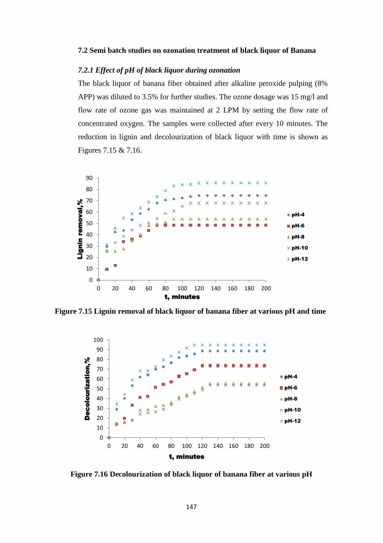
147
7.2 Semi batch studies on ozonation treatment of black liquor of Banana
7.2.1 Effect of pH of black liquor during ozonation
The black liquor of banana fiber obtained after alkaline peroxide pulping (8%
APP) was diluted to 3.5% for further studies. The ozone dosage was 15 mg/l and
flow rate of ozone gas was maintained at 2 LPM by setting the flow rate of
concentrated oxygen. The samples were collected after every 10 minutes. The
reduction in lignin and decolourization of black liquor with time is shown as
Figures 7.15 & 7.16.
Figure 7.15 Lignin removal of black liquor of banana fiber at various pH and time
Figure 7.16 Decolourization of black liquor of banana fiber at various pH
0
10
20
30
40
50
60
70
80
90
0 20 40 60 80 100 120 140 160 180 200
Lignin re
moval,%
t, minutes
pH-4
pH-6
pH-8
pH-10
pH-12
0
10
20
30
40
50
60
70
80
90
100
0 20 40 60 80 100 120 140 160 180 200
Decolourization,%
t, minutes
pH-4
pH-6
pH-8
pH-10
pH-12
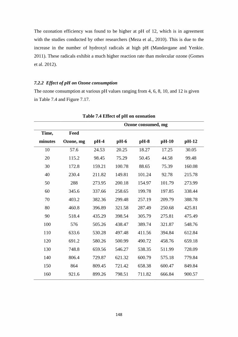
148
The ozonation efficiency was found to be higher at pH of 12, which is in agreement
with the studies conducted by other researchers (Meza et al., 2010). This is due to the
increase in the number of hydroxyl radicals at high pH (Mandavgane and Yenkie.
2011). These radicals exhibit a much higher reaction rate than molecular ozone (Gomes
et al. 2012).
7.2.2 Effect of pH on Ozone consumption
The ozone consumption at various pH values ranging from 4, 6, 8, 10, and 12 is given
in Table 7.4 and Figure 7.17.
Table 7.4 Effect of pH on ozonation
Ozone consumed, mg
Time,
minutes
Feed
Ozone, mg pH-4 pH-6 pH-8 pH-10 pH-12
10 57.6 24.53 20.25 18.27 17.25 30.05
20 115.2 98.45 75.29 50.45 44.58 99.48
30 172.8 159.21 100.78 88.65 75.39 160.08
40 230.4 211.82 149.81 101.24 92.78 215.78
50 288 273.95 200.18 154.97 101.79 273.99
60 345.6 337.66 258.65 199.78 197.85 338.44
70 403.2 382.36 299.48 257.19 209.79 388.78
80 460.8 396.89 321.58 287.49 250.68 425.81
90 518.4 435.29 398.54 305.79 275.81 475.49
100 576 505.26 438.47 389.74 321.87 548.76
110 633.6 530.28 497.48 411.56 394.84 612.84
120 691.2 580.26 500.99 490.72 458.76 659.18
130 748.8 659.56 546.27 538.35 511.99 728.09
140 806.4 729.87 621.32 600.79 575.18 779.84
150 864 809.45 721.42 658.38 600.47 849.84
160 921.6 899.26 798.51 711.82 666.84 900.57
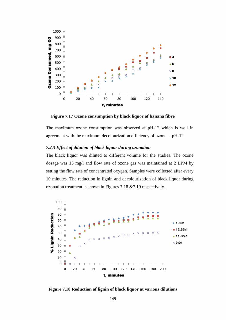
149
Figure 7.17 Ozone consumption by black liquor of banana fibre
The maximum ozone consumption was observed at pH-12 which is well in
agreement with the maximum decolourization efficiency of ozone at pH-12.
7.2.3 Effect of dilution of black liquor during ozonation
The black liquor was diluted to different volume for the studies. The ozone
dosage was 15 mg/l and flow rate of ozone gas was maintained at 2 LPM by
setting the flow rate of concentrated oxygen. Samples were collected after every
10 minutes. The reduction in lignin and decolourization of black liquor during
ozonation treatment is shown in Figures 7.18 &7.19 respectively.
Figure 7.18 Reduction of lignin of black liquor at various dilutions
0
100
200
300
400
500
600
700
800
900
1000
0 20 40 60 80 100 120 140
Ozone C
onsum
ed, m
g O
3
t, minutes
4
6
8
10
12
0
10
20
30
40
50
60
70
80
90
100
0 20 40 60 80 100 120 140 160 180 200
% Lignin R
eduction
t, minutes
19:01
12.33:1
11.85:1
9:01
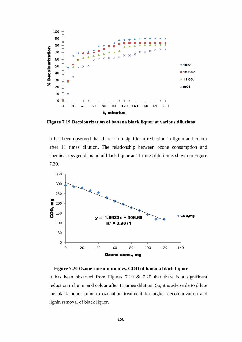
150
Figure 7.19 Decolourization of banana black liquor at various dilutions
It has been observed that there is no significant reduction in lignin and colour
after 11 times dilution. The relationship between ozone consumption and
chemical oxygen demand of black liquor at 11 times dilution is shown in Figure
7.20.
Figure 7.20 Ozone consumption vs. COD of banana black liquor
It has been observed from Figures 7.19 & 7.20 that there is a significant
reduction in lignin and colour after 11 times dilution. So, it is advisable to dilute
the black liquor prior to ozonation treatment for higher decolourization and
lignin removal of black liquor.
0
10
20
30
40
50
60
70
80
90
100
0 20 40 60 80 100 120 140 160 180 200
% D
ecolourization
t, minutes
19:01
12.33:1
11.85:1
9:01
y = -1.5923x + 306.69
R² = 0.9871
0
50
100
150
200
250
300
350
0 20 40 60 80 100 120 140
CO
D, m
g
Ozone cons., mg
COD,mg
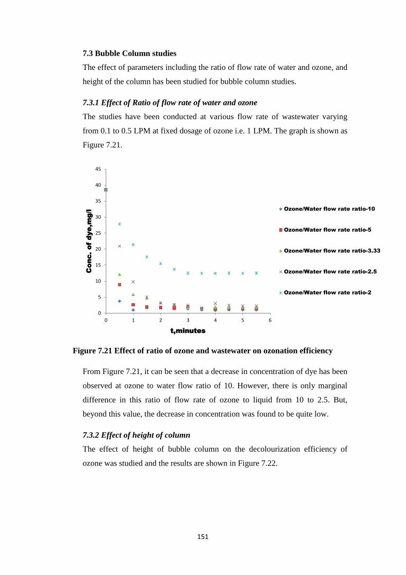
151
7.3 Bubble Column studies
The effect of parameters including the ratio of flow rate of water and ozone, and
height of the column has been studied for bubble column studies.
7.3.1 Effect of Ratio of flow rate of water and ozone
The studies have been conducted at various flow rate of wastewater varying
from 0.1 to 0.5 LPM at fixed dosage of ozone i.e. 1 LPM. The graph is shown as
Figure 7.21.
Figure 7.21 Effect of ratio of ozone and wastewater on ozonation efficiency
From Figure 7.21, it can be seen that a decrease in concentration of dye has been
observed at ozone to water flow ratio of 10. However, there is only marginal
difference in this ratio of flow rate of ozone to liquid from 10 to 2.5. But,
beyond this value, the decrease in concentration was found to be quite low.
7.3.2 Effect of height of column
The effect of height of bubble column on the decolourization efficiency of
ozone was studied and the results are shown in Figure 7.22.
0
5
10
15
20
25
30
35
40
45
0 1 2 3 4 5 6
Conc. of dye,m
g/l
t,minutes
Ozone/Water flow rate ratio-10
Ozone/Water flow rate ratio-5
Ozone/Water flow rate ratio-3.33
Ozone/Water flow rate ratio-2.5
Ozone/Water flow rate ratio-2
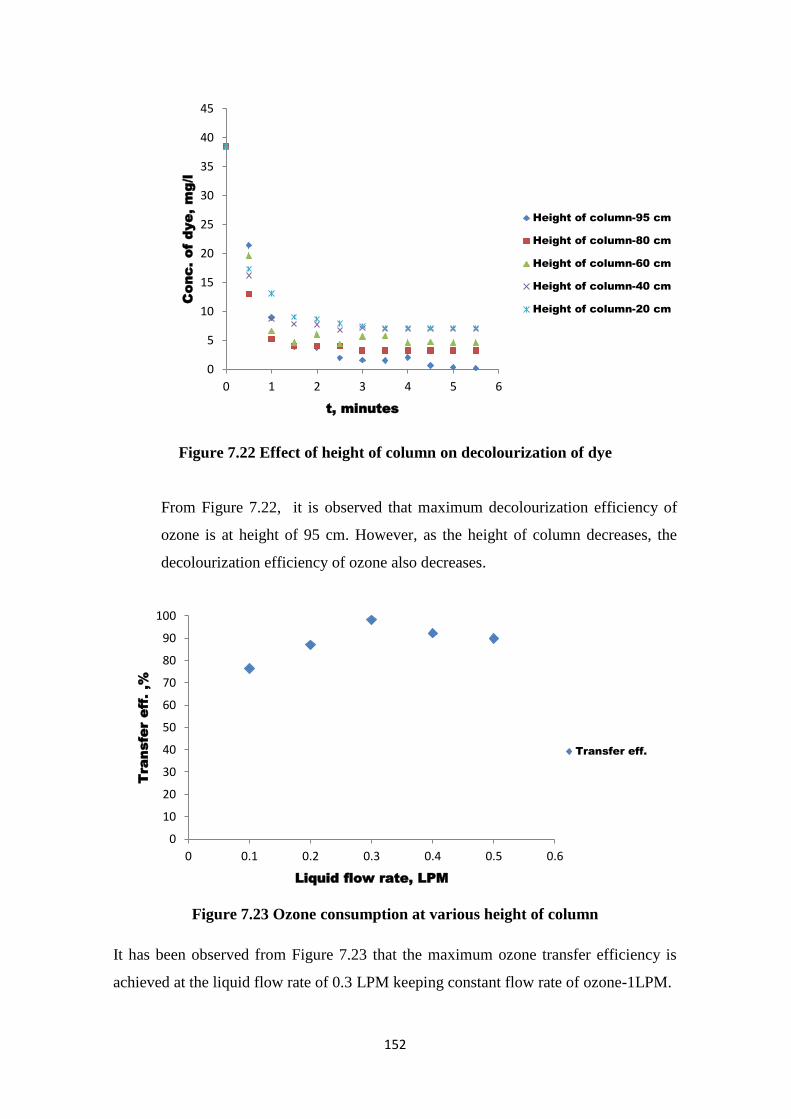
152
Figure 7.22 Effect of height of column on decolourization of dye
From Figure 7.22, it is observed that maximum decolourization efficiency of
ozone is at height of 95 cm. However, as the height of column decreases, the
decolourization efficiency of ozone also decreases.
Figure 7.23 Ozone consumption at various height of column
It has been observed from Figure 7.23 that the maximum ozone transfer efficiency is
achieved at the liquid flow rate of 0.3 LPM keeping constant flow rate of ozone-1LPM.
0
5
10
15
20
25
30
35
40
45
0 1 2 3 4 5 6
Conc. of dye, m
g/l
t, minutes
Height of column-95 cm
Height of column-80 cm
Height of column-60 cm
Height of column-40 cm
Height of column-20 cm
0
10
20
30
40
50
60
70
80
90
100
0 0.1 0.2 0.3 0.4 0.5 0.6
Tra
nsfer eff. ,%
Liquid flow rate, LPM
Transfer eff.
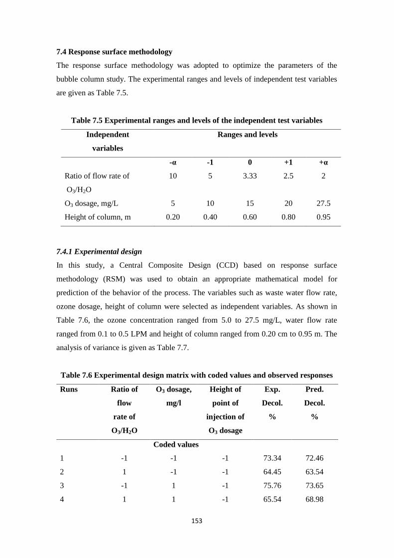
153
7.4 Response surface methodology
The response surface methodology was adopted to optimize the parameters of the
bubble column study. The experimental ranges and levels of independent test variables
are given as Table 7.5.
Table 7.5 Experimental ranges and levels of the independent test variables
Independent
variables
Ranges and levels
-α -1 0 +1 +α
Ratio of flow rate of
O3/H2O
10 5 3.33 2.5 2
O3 dosage, mg/L 5 10 15 20 27.5
Height of column, m 0.20 0.40 0.60 0.80 0.95
7.4.1 Experimental design
In this study, a Central Composite Design (CCD) based on response surface
methodology (RSM) was used to obtain an appropriate mathematical model for
prediction of the behavior of the process. The variables such as waste water flow rate,
ozone dosage, height of column were selected as independent variables. As shown in
Table 7.6, the ozone concentration ranged from 5.0 to 27.5 mg/L, water flow rate
ranged from 0.1 to 0.5 LPM and height of column ranged from 0.20 cm to 0.95 m. The
analysis of variance is given as Table 7.7.
Table 7.6 Experimental design matrix with coded values and observed responses
Runs Ratio of
flow
rate of
O3/H2O
O3 dosage,
mg/l
Height of
point of
injection of
O3 dosage
Exp.
Decol.
%
Pred.
Decol.
%
Coded values
1 -1 -1 -1 73.34 72.46
2 1 -1 -1 64.45 63.54
3 -1 1 -1 75.76 73.65
4 1 1 -1 65.54 68.98
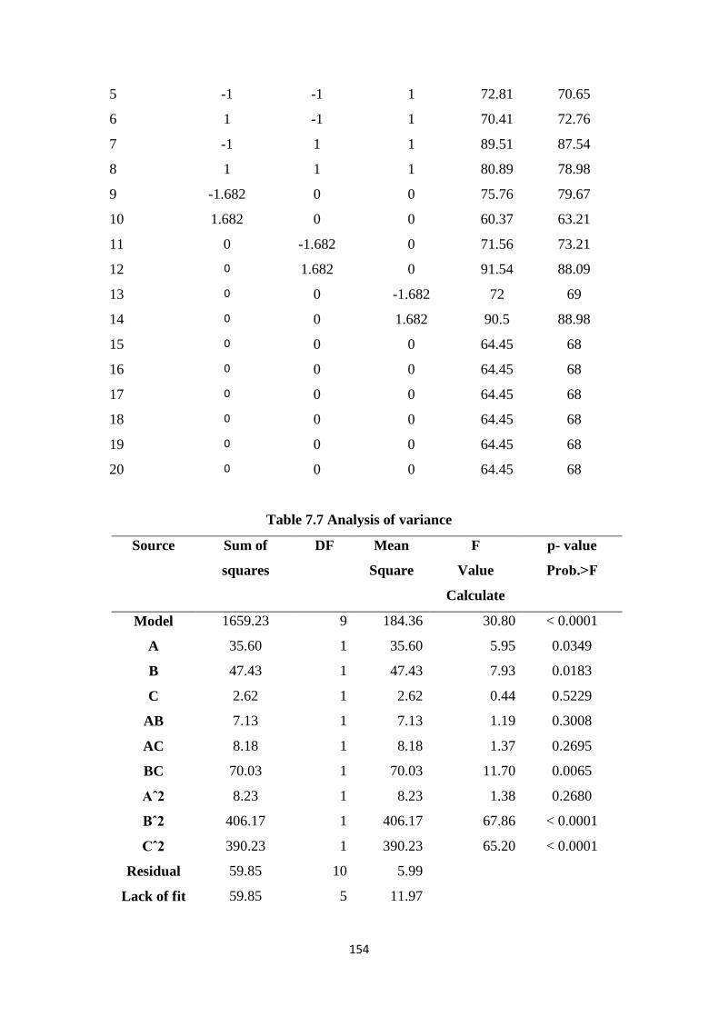
154
5 -1 -1 1 72.81 70.65
6 1 -1 1 70.41 72.76
7 -1 1 1 89.51 87.54
8 1 1 1 80.89 78.98
9 -1.682 0 0 75.76 79.67
10 1.682 0 0 60.37 63.21
11 0 -1.682 0 71.56 73.21
12 0 1.682 0 91.54 88.09
13 0 0 -1.682 72 69
14 0 0 1.682 90.5 88.98
15 0 0 0 64.45 68
16 0 0 0 64.45 68
17 0 0 0 64.45 68
18 0 0 0 64.45 68
19 0 0 0 64.45 68
20 0 0 0 64.45 68
Table 7.7 Analysis of variance
Source Sum of
squares
DF Mean
Square
F
Value
Calculate
p- value
Prob.˃F
Model 1659.23 9 184.36 30.80 < 0.0001
A 35.60 1 35.60 5.95 0.0349
B 47.43 1 47.43 7.93 0.0183
C 2.62 1 2.62 0.44 0.5229
AB 7.13 1 7.13 1.19 0.3008
AC 8.18 1 8.18 1.37 0.2695
BC 70.03 1 70.03 11.70 0.0065
Aˆ2 8.23 1 8.23 1.38 0.2680
Bˆ2 406.17 1 406.17 67.86 < 0.0001
Cˆ2 390.23 1 390.23 65.20 < 0.0001
Residual 59.85 10 5.99
Lack of fit 59.85 5 11.97
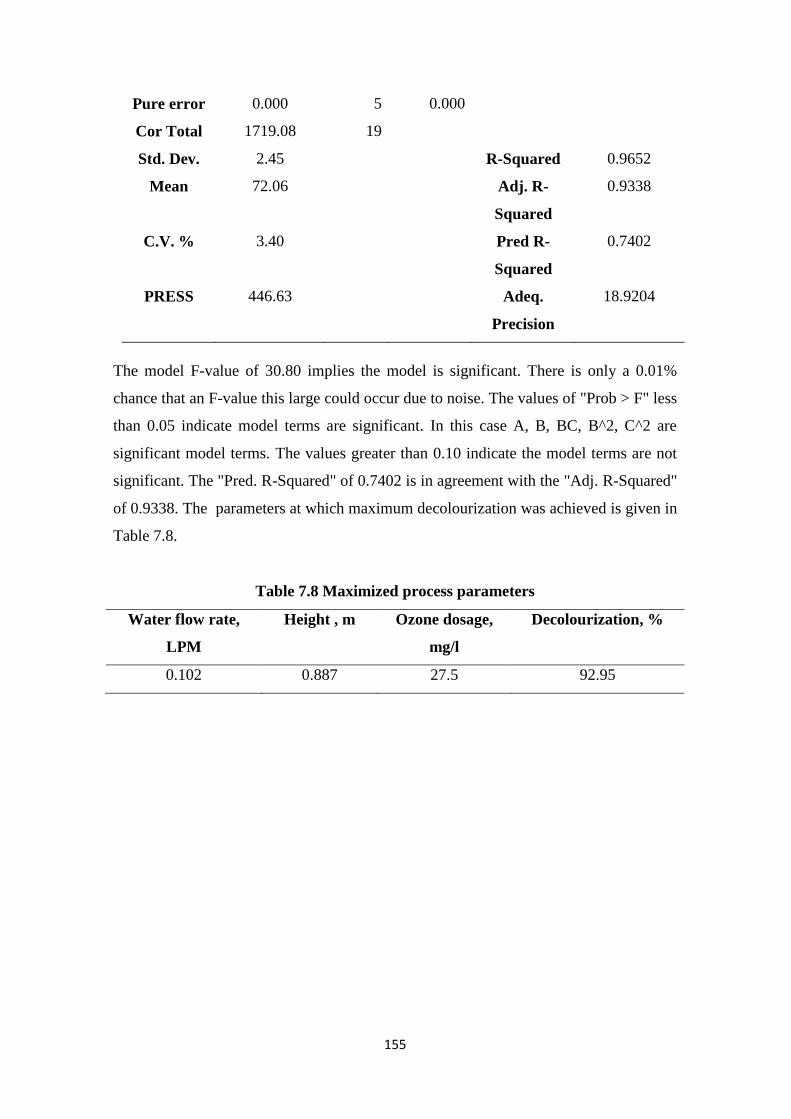
155
Pure error 0.000 5 0.000
Cor Total 1719.08 19
Std. Dev. 2.45 R-Squared 0.9652
Mean 72.06 Adj. R-
Squared
0.9338
C.V. % 3.40 Pred R-
Squared
0.7402
PRESS 446.63 Adeq.
Precision
18.9204
The model F-value of 30.80 implies the model is significant. There is only a 0.01%
chance that an F-value this large could occur due to noise. The values of "Prob > F" less
than 0.05 indicate model terms are significant. In this case A, B, BC, B^2, C^2 are
significant model terms. The values greater than 0.10 indicate the model terms are not
significant. The "Pred. R-Squared" of 0.7402 is in agreement with the "Adj. R-Squared"
of 0.9338. The parameters at which maximum decolourization was achieved is given in
Table 7.8.
Table 7.8 Maximized process parameters
Water flow rate,
LPM
Height , m Ozone dosage,
mg/l
Decolourization, %
0.102 0.887 27.5 92.95
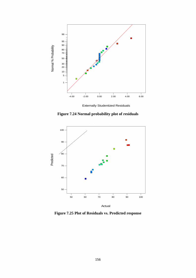
156
Figure 7.24 Normal probability plot of residuals
Figure 7.25 Plot of Residuals vs. Predicted response
Design-Expert® SoftwareDecolorization
Color points by value ofDecolorization:
91.54
60.37
Externally Studentized Residuals
Norm
al %
Pro
babili
ty
Normal Plot of Residuals
-4.00 -2.00 0.00 2.00 4.00 6.00
1
5
10
20
30
50
70
80
90
95
99
Design-Expert® SoftwareDecolorization
Color points by value ofDecolorization:
91.54
60.37
Actual
Pre
dict
ed
Predicted vs. Actual
50
60
70
80
90
100
50 60 70 80 90 100
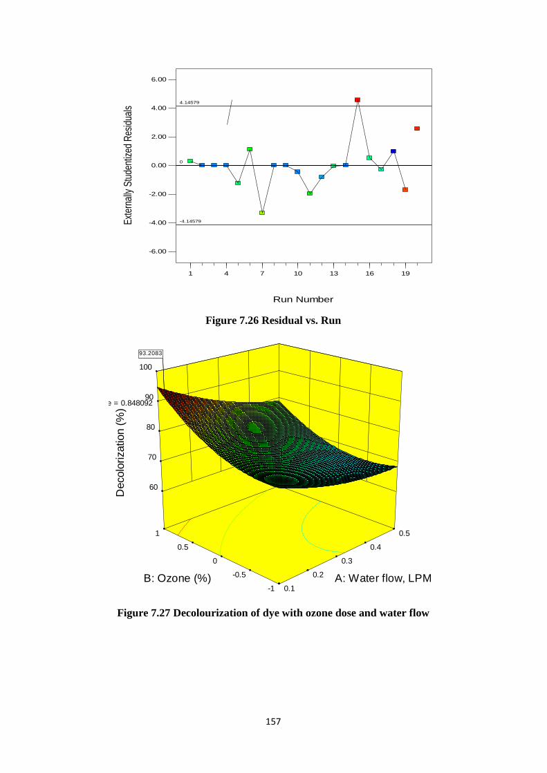
157
Figure 7.26 Residual vs. Run
Figure 7.27 Decolourization of dye with ozone dose and water flow
Design-Expert® SoftwareDecolorization
Color points by value ofDecolorization:
91.54
60.37
Run Number
Ext
erna
lly S
tude
ntiz
ed R
esid
uals
Residuals vs. Run
-6.00
-4.00
-2.00
0.00
2.00
4.00
6.00
1 4 7 10 13 16 19
4.14579
-4.14579
0
Design-Expert® SoftwareFactor Coding: ActualDecolorization (%)
91.54
60.37
X1 = A: Water flow, LPMX2 = B: Ozone
Actual FactorC: Height of injection of ozone = 0.848092
-1
-0.5
0
0.5
1
0.1
0.2
0.3
0.4
0.5
60
70
80
90
100
Decolo
rization (
%)
A: Water flow, LPMB: Ozone (%)
93.208393.2083
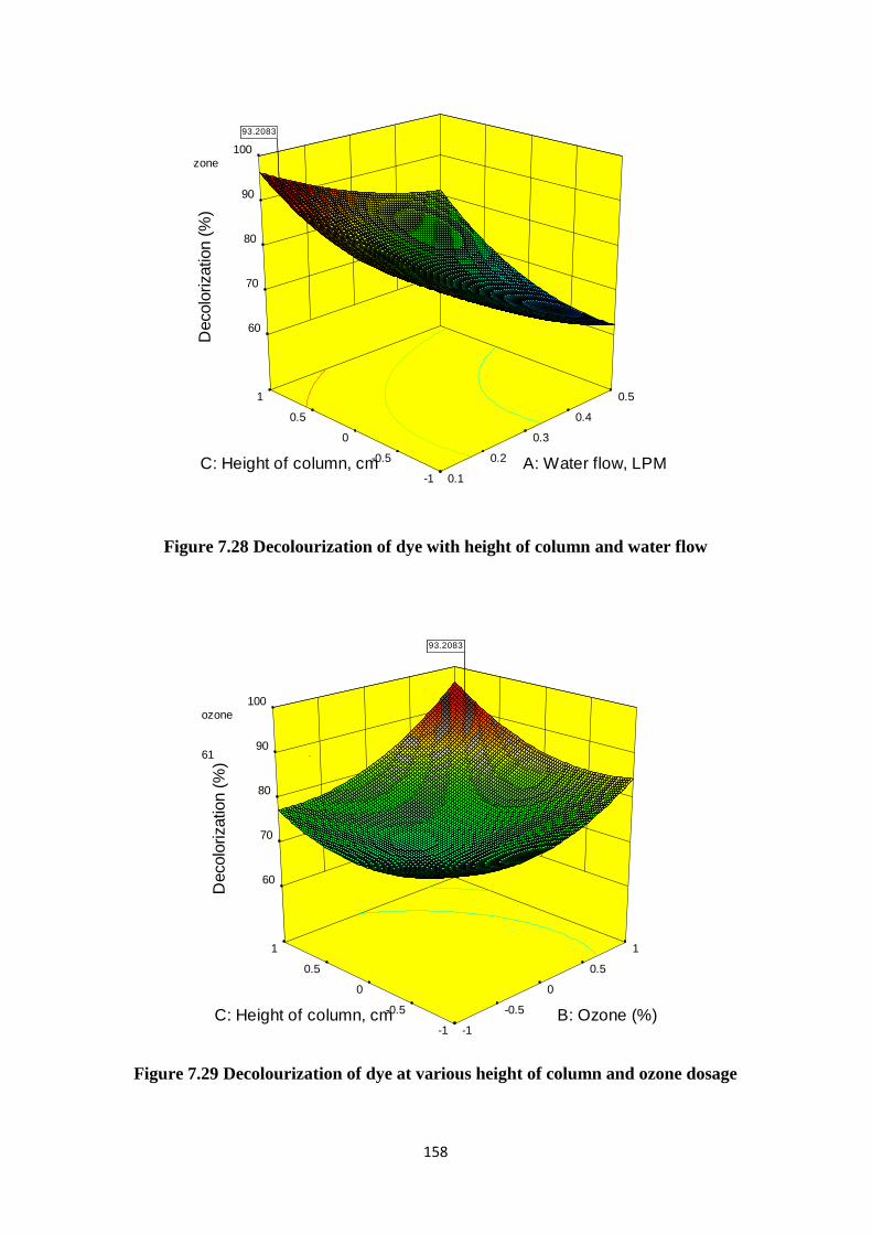
158
Figure 7.28 Decolourization of dye with height of column and water flow
Figure 7.29 Decolourization of dye at various height of column and ozone dosage
Design-Expert® SoftwareFactor Coding: ActualDecolorization (%)
91.54
60.37
X1 = A: Water flow, LPMX2 = C: Height of injection of ozone
Actual FactorB: Ozone = 0.961508
-1
-0.5
0
0.5
1
0.1
0.2
0.3
0.4
0.5
60
70
80
90
100
Decolo
rization (
%)
A: Water flow, LPMC: Height of column, cm
93.208393.2083
Design-Expert® SoftwareFactor Coding: ActualDecolorization (%)
91.54
60.37
X1 = B: OzoneX2 = C: Height of injection of ozone
Actual FactorA: Water flow, LPM = 0.114361
-1
-0.5
0
0.5
1
-1
-0.5
0
0.5
1
60
70
80
90
100
Decolo
rization (
%)
B: Ozone (%)C: Height of column, cm
93.208393.2083
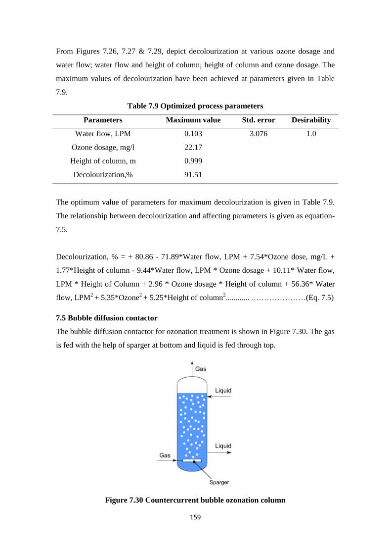
159
From Figures 7.26, 7.27 & 7.29, depict decolourization at various ozone dosage and
water flow; water flow and height of column; height of column and ozone dosage. The
maximum values of decolourization have been achieved at parameters given in Table
7.9.
Table 7.9 Optimized process parameters
Parameters Maximum value Std. error Desirability
Water flow, LPM 0.103 3.076 1.0
Ozone dosage, mg/l 22.17
Height of column, m 0.999
Decolourization,% 91.51
The optimum value of parameters for maximum decolourization is given in Table 7.9.
The relationship between decolourization and affecting parameters is given as equation-
7.5.
Decolourization, % = + 80.86 - 71.89*Water flow, LPM + 7.54*Ozone dose, mg/L +
1.77*Height of column - 9.44*Water flow, LPM * Ozone dosage + 10.11* Water flow,
LPM * Height of Column + 2.96 * Ozone dosage * Height of column + 56.36* Water
flow, LPM2
+ 5.35*Ozone2
+ 5.25*Height of column2............
…………………(Eq. 7.5)
7.5 Bubble diffusion contactor
The bubble diffusion contactor for ozonation treatment is shown in Figure 7.30. The gas
is fed with the help of sparger at bottom and liquid is fed through top.
Figure 7.30 Countercurrent bubble ozonation column
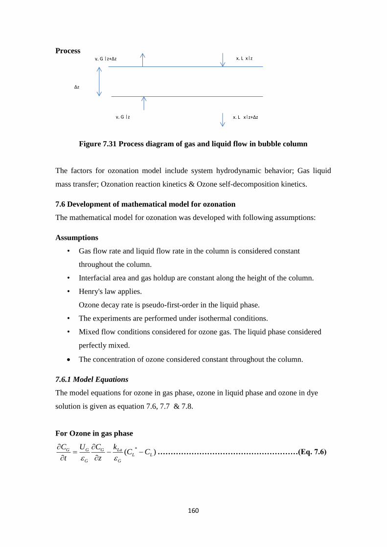
160
Process
Figure 7.31 Process diagram of gas and liquid flow in bubble column
The factors for ozonation model include system hydrodynamic behavior; Gas liquid
mass transfer; Ozonation reaction kinetics & Ozone self-decomposition kinetics.
7.6 Development of mathematical model for ozonation
The mathematical model for ozonation was developed with following assumptions:
Assumptions
• Gas flow rate and liquid flow rate in the column is considered constant
throughout the column.
• Interfacial area and gas holdup are constant along the height of the column.
• Henry's law applies.
Ozone decay rate is pseudo-first-order in the liquid phase.
• The experiments are performed under isothermal conditions.
• Mixed flow conditions considered for ozone gas. The liquid phase considered
perfectly mixed.
The concentration of ozone considered constant throughout the column.
7.6.1 Model Equations
The model equations for ozone in gas phase, ozone in liquid phase and ozone in dye
solution is given as equation 7.6, 7.7 & 7.8.
For Ozone in gas phase
)(*
LL
G
LaG
G
GG CCk
z
CU
t
C
………………………………………………(Eq. 7.6)
y, G │z
x, L x│z y, G │z+∆z
x, L x│z+∆z
∆z
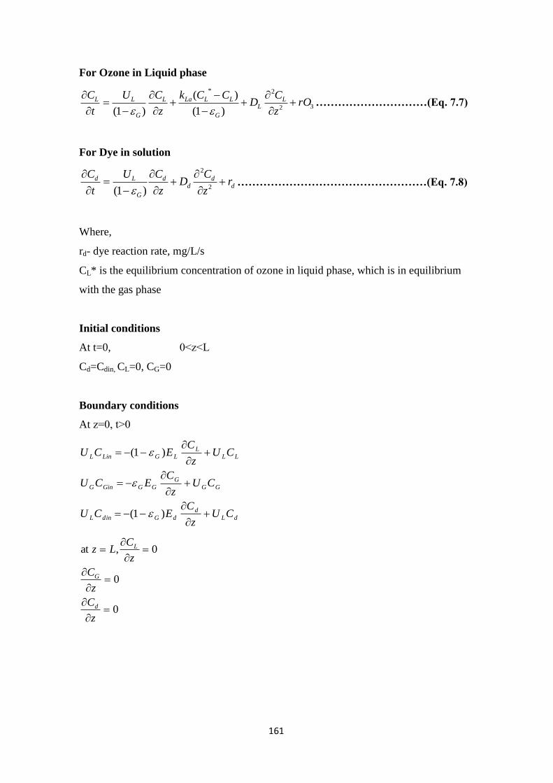
161
For Ozone in Liquid phase
32
2*
)1(
)(
)1(rO
z
CD
CCk
z
CU
t
C LL
G
LLLaL
G
LL
…………………………(Eq. 7.7)
For Dye in solution
dd
dd
G
Ld rz
CD
z
CU
t
C
2
2
)1( ……………………………………………(Eq. 7.8)
Where,
rd- dye reaction rate, mg/L/s
CL* is the equilibrium concentration of ozone in liquid phase, which is in equilibrium
with the gas phase
Initial conditions
At t=0, 0˂z˂L
Cd=Cdin, CL=0, CG=0
Boundary conditions
At z=0, t˃0
dL
d
dGdinL
GG
G
GGGinG
LL
L
LGLinL
CUz
CECU
CUz
CECU
CUz
CECU
)1(
)1(
0
0
0,at
z
C
z
C
z
CLz
d
G
L
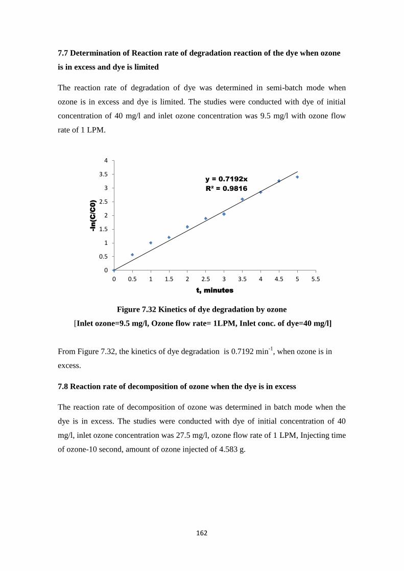
162
7.7 Determination of Reaction rate of degradation reaction of the dye when ozone
is in excess and dye is limited
The reaction rate of degradation of dye was determined in semi-batch mode when
ozone is in excess and dye is limited. The studies were conducted with dye of initial
concentration of 40 mg/l and inlet ozone concentration was 9.5 mg/l with ozone flow
rate of 1 LPM.
Figure 7.32 Kinetics of dye degradation by ozone
[Inlet ozone=9.5 mg/l, Ozone flow rate= 1LPM, Inlet conc. of dye=40 mg/l]
From Figure 7.32, the kinetics of dye degradation is 0.7192 min-1
, when ozone is in
excess.
7.8 Reaction rate of decomposition of ozone when the dye is in excess
The reaction rate of decomposition of ozone was determined in batch mode when the
dye is in excess. The studies were conducted with dye of initial concentration of 40
mg/l, inlet ozone concentration was 27.5 mg/l, ozone flow rate of 1 LPM, Injecting time
of ozone-10 second, amount of ozone injected of 4.583 g.
y = 0.7192x
R² = 0.9816
0
0.5
1
1.5
2
2.5
3
3.5
4
0 0.5 1 1.5 2 2.5 3 3.5 4 4.5 5 5.5
-ln(C
/C
0)
t, minutes
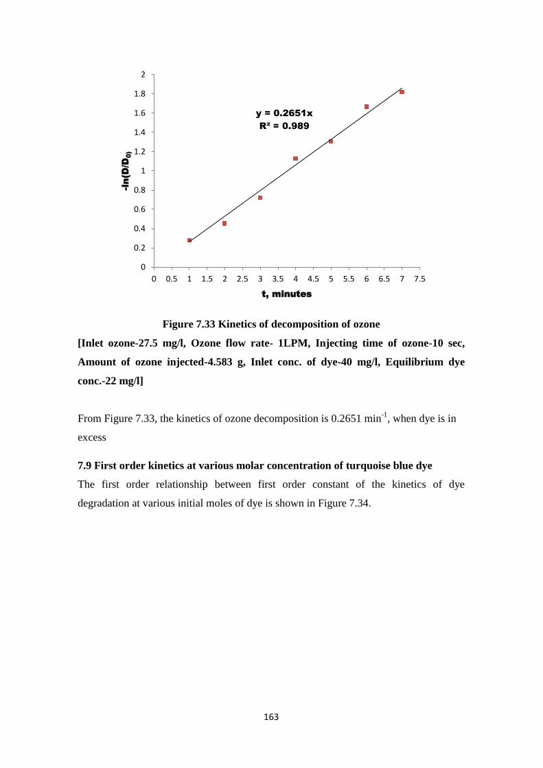
163
Figure 7.33 Kinetics of decomposition of ozone
[Inlet ozone-27.5 mg/l, Ozone flow rate- 1LPM, Injecting time of ozone-10 sec,
Amount of ozone injected-4.583 g, Inlet conc. of dye-40 mg/l, Equilibrium dye
conc.-22 mg/l]
From Figure 7.33, the kinetics of ozone decomposition is 0.2651 min-1
, when dye is in
excess
7.9 First order kinetics at various molar concentration of turquoise blue dye
The first order relationship between first order constant of the kinetics of dye
degradation at various initial moles of dye is shown in Figure 7.34.
y = 0.2651x
R² = 0.989
0
0.2
0.4
0.6
0.8
1
1.2
1.4
1.6
1.8
2
0 0.5 1 1.5 2 2.5 3 3.5 4 4.5 5 5.5 6 6.5 7 7.5
-ln(D
/D
0)
t, minutes
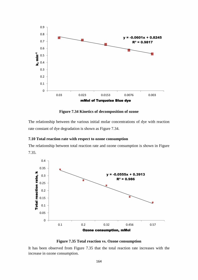
164
Figure 7.34 Kinetics of decomposition of ozone
The relationship between the various initial molar concentrations of dye with reaction
rate constant of dye degradation is shown as Figure 7.34.
7.10 Total reaction rate with respect to ozone consumption
The relationship between total reaction rate and ozone consumption is shown in Figure
7.35.
Figure 7.35 Total reaction vs. Ozone consumption
It has been observed from Figure 7.35 that the total reaction rate increases with the
increase in ozone consumption.
y = -0.0601x + 0.8245
R² = 0.9817
0
0.1
0.2
0.3
0.4
0.5
0.6
0.7
0.8
0.9
0.03 0.023 0.0153 0.0076 0.003
k, m
in
-1
mMol of Turquoise Blue dye
y = -0.0555x + 0.3913
R² = 0.986
0
0.05
0.1
0.15
0.2
0.25
0.3
0.35
0.4
0.1 0.2 0.32 0.456 0.57
Tota
l re
action ra
te, k
Ozone consumption, mMol
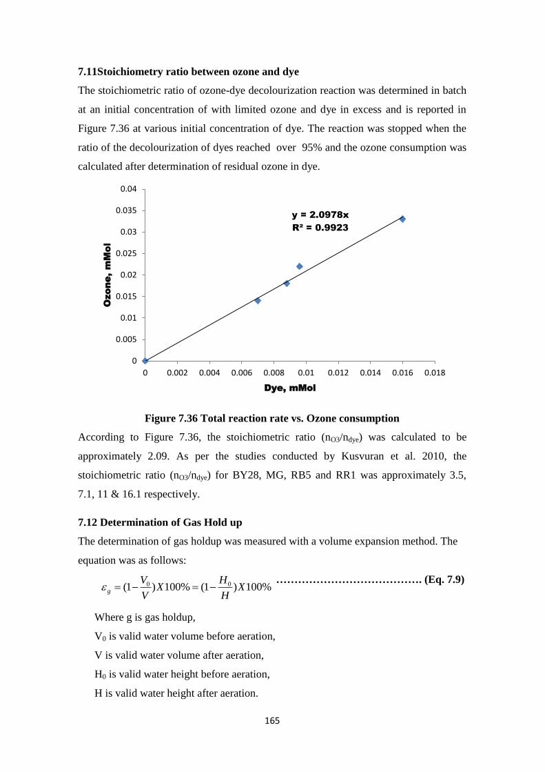
165
7.11Stoichiometry ratio between ozone and dye
The stoichiometric ratio of ozone-dye decolourization reaction was determined in batch
at an initial concentration of with limited ozone and dye in excess and is reported in
Figure 7.36 at various initial concentration of dye. The reaction was stopped when the
ratio of the decolourization of dyes reached over 95% and the ozone consumption was
calculated after determination of residual ozone in dye.
Figure 7.36 Total reaction rate vs. Ozone consumption
According to Figure 7.36, the stoichiometric ratio (nO3/ndye) was calculated to be
approximately 2.09. As per the studies conducted by Kusvuran et al. 2010, the
stoichiometric ratio (nO3/ndye) for BY28, MG, RB5 and RR1 was approximately 3.5,
7.1, 11 & 16.1 respectively.
7.12 Determination of Gas Hold up
The determination of gas holdup was measured with a volume expansion method. The
equation was as follows:
…………………………………. (Eq. 7.9)
Where g is gas holdup,
V0 is valid water volume before aeration,
V is valid water volume after aeration,
H0 is valid water height before aeration,
H is valid water height after aeration.
y = 2.0978x
R² = 0.9923
0
0.005
0.01
0.015
0.02
0.025
0.03
0.035
0.04
0 0.002 0.004 0.006 0.008 0.01 0.012 0.014 0.016 0.018
Ozone, m
Mol
Dye, mMol
%100)1(%100)1( 00 XH
HX
V
Vg
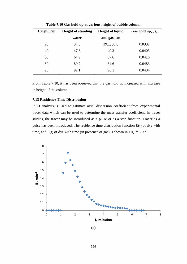
166
Table 7.10 Gas hold up at various height of bubble column
Height, cm Height of standing
water
Height of liquid
and gas, cm
Gas hold up, , εg
20 37.8 39.1, 38.8 0.0332
40 47.3 49.3 0.0405
60 64.9 67.6 0.0416
80 80.7 84.6 0.0483
95 92.1 96.1 0.0434
From Table 7.10, it has been observed that the gas hold up increased with increase
in height of the column.
7.13 Residence Time Distribution
RTD analysis is used to estimate axial dispersion coefficient from experimental
tracer data which can be used to determine the mass transfer coefficient. In tracer
studies, the tracer may be introduced as a pulse or as a step function. Tracer as a
pulse has been introduced. The residence time distribution function E(t) of dye with
time, and E(t) of dye with time (in presence of gas) is shown in Figure 7.37.
(a)
0
0.1
0.2
0.3
0.4
0.5
0.6
0.7
0.8
0 1 2 3 4 5 6 7 8
E, m
in
-1
t, minutes
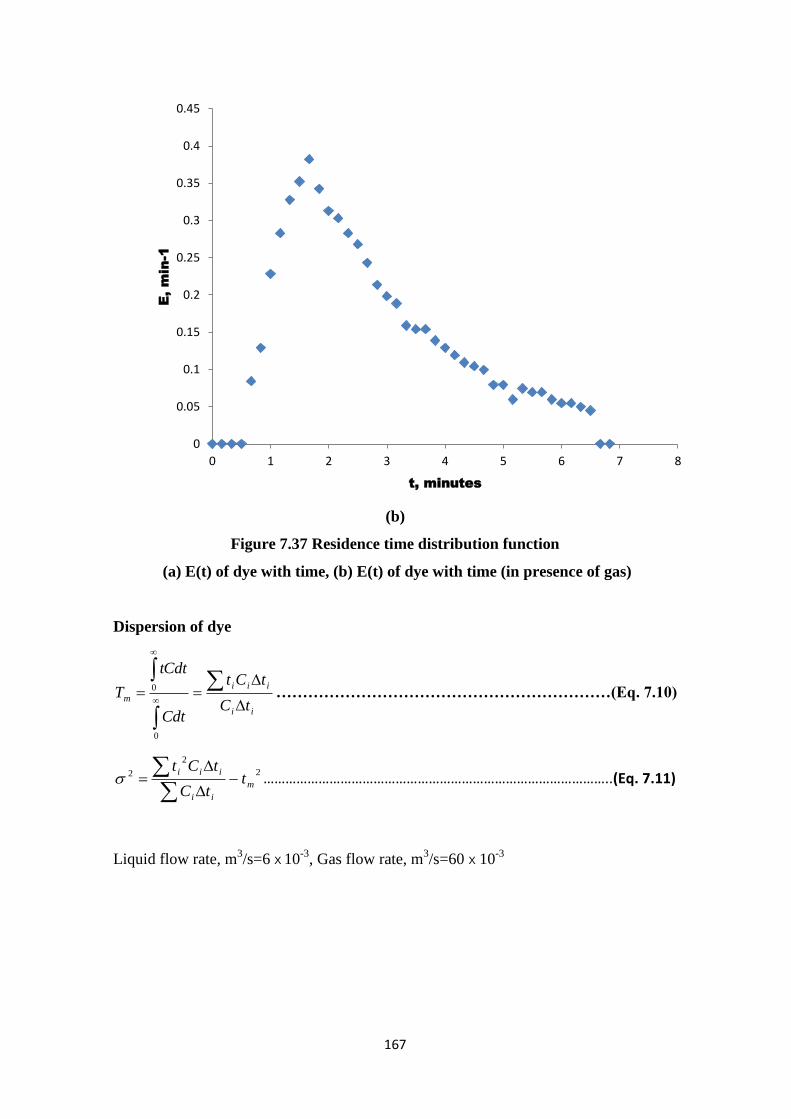
167
(b)
Figure 7.37 Residence time distribution function
(a) E(t) of dye with time, (b) E(t) of dye with time (in presence of gas)
Dispersion of dye
ii
iii
mtC
tCt
Cdt
tCdt
T
0
0 ………………………………………………………(Eq. 7.10)
2
2
2
m
ii
iiit
tC
tCt
…………………………………………………………………………………..(Eq. 7.11)
Liquid flow rate, m3/s=6 X 10
-3, Gas flow rate, m
3/s=60 X 10
-3
0
0.05
0.1
0.15
0.2
0.25
0.3
0.35
0.4
0.45
0 1 2 3 4 5 6 7 8
E, m
in
-1
t, minutes
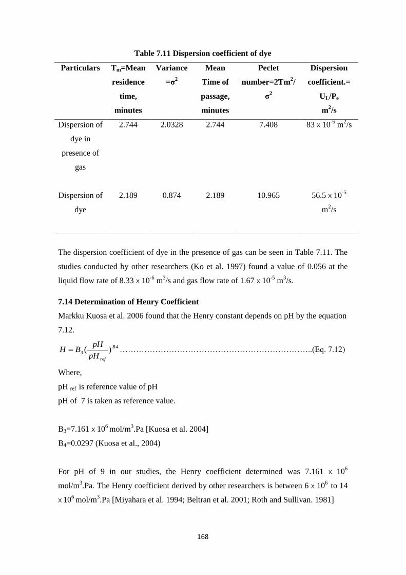
168
Table 7.11 Dispersion coefficient of dye
Particulars Tm=Mean
residence
time,
minutes
Variance
=σ2
Mean
Time of
passage,
minutes
Peclet
number=2Tm2/
σ2
Dispersion
coefficient.=
UL/Pe
m2/s
Dispersion of
dye in
presence of
gas
2.744 2.0328 2.744 7.408 83 X 10-5
m2/s
Dispersion of
dye
2.189 0.874 2.189 10.965 56.5 X 10⁻⁵
m2/s
The dispersion coefficient of dye in the presence of gas can be seen in Table 7.11. The
studies conducted by other researchers (Ko et al. 1997) found a value of 0.056 at the
liquid flow rate of 8.33 X 10⁻⁶
m3/s and gas flow rate of 1.67 X 10
-5 m
3/s.
7.14 Determination of Henry Coefficient
Markku Kuosa et al. 2006 found that the Henry constant depends on pH by the equation
7.12.
4
3 )( B
refpH
pHBH ……………………………………………………………..(Eq. 7.12)
Where,
pH ref is reference value of pH
pH of 7 is taken as reference value.
B3=7.161 X 10⁶
mol/m3.Pa [Kuosa et al. 2004]
B4=0.0297 (Kuosa et al., 2004)
For pH of 9 in our studies, the Henry coefficient determined was 7.161 X 10⁶
mol/m3.Pa. The Henry coefficient derived by other researchers is between 6 X 10
6 to 14
X 106
mol/m3.Pa [Miyahara et al. 1994; Beltran et al. 2001; Roth and Sullivan. 1981]
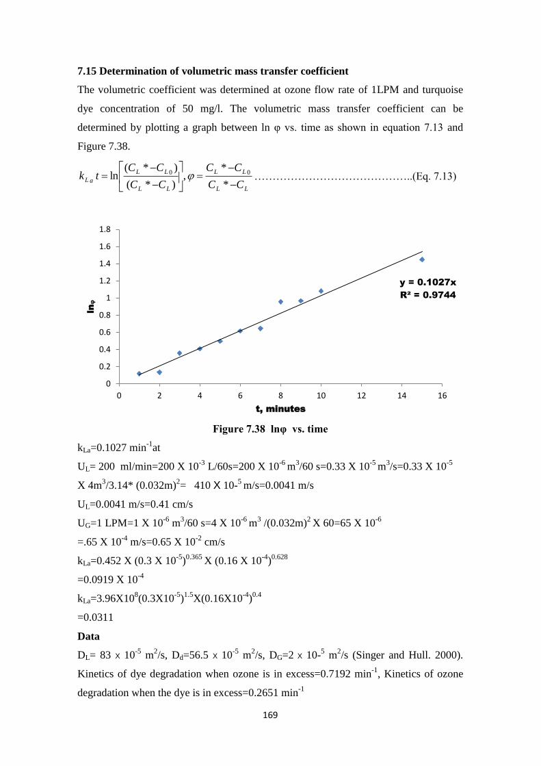
169
7.15 Determination of volumetric mass transfer coefficient
The volumetric coefficient was determined at ozone flow rate of 1LPM and turquoise
dye concentration of 50 mg/l. The volumetric mass transfer coefficient can be
determined by plotting a graph between ln φ vs. time as shown in equation 7.13 and
Figure 7.38.
LL
LL
LL
LL
aLCC
CC
CC
CCtk
*
*,
)*(
)*(ln 00 ……………………………………..(Eq. 7.13)
Figure 7.38 lnφ vs. time
kLa=0.1027 min-1
at
UL= 200 ml/min=200 X 10-3
L/60s=200 X 10-6
m3/60 s=0.33 X 10
-5 m
3/s=0.33 X 10
-5
X 4m3/3.14* (0.032m)
2= 410 X 10-
5 m/s=0.0041 m/s
UL=0.0041 m/s=0.41 cm/s
UG=1 LPM=1 X 10⁻⁶
m3/60 s=4 X 10
-6 m
3 /(0.032m)
2 X 60=65 X 10
-6
=.65 X 10-4
m/s=0.65 X 10-2
cm/s
kLa=0.452 X (0.3 X 10-5
)0.365
X (0.16 X 10-4
)0.628
=0.0919 X 10⁻⁴
kLa=3.96X10⁸(0.3X10
-5)1.5
X(0.16X10-4
)0.4
=0.0311
Data
DL= 83 X 10-5
m2/s, Dd=56.5 X 10
-5 m
2/s, DG=2 X 10-
5 m
2/s (Singer and Hull. 2000).
Kinetics of dye degradation when ozone is in excess=0.7192 min-1
, Kinetics of ozone
degradation when the dye is in excess=0.2651 min-1
y = 0.1027x
R² = 0.9744
0
0.2
0.4
0.6
0.8
1
1.2
1.4
1.6
1.8
0 2 4 6 8 10 12 14 16
lnᵩ
t, minutes
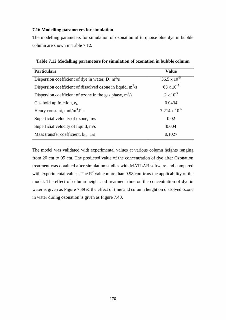
170
7.16 Modelling parameters for simulation
The modelling parameters for simulation of ozonation of turquoise blue dye in bubble
column are shown in Table 7.12.
Table 7.12 Modelling parameters for simulation of ozonation in bubble column
Particulars Value
Dispersion coefficient of dye in water, Dd m2/s 56.5 X 10
-5
Dispersion coefficient of dissolved ozone in liquid, m2/s 83 X 10
-5
Dispersion coefficient of ozone in the gas phase, m2/s 2 X 10
-5
Gas hold up fraction, εG 0.0434
Henry constant, mol/m3.Pa 7.214 X 10
6
Superficial velocity of ozone, m/s 0.02
Superficial velocity of liquid, m/s 0.004
Mass transfer coefficient, kLa, 1/s 0.1027
The model was validated with experimental values at various column heights ranging
from 20 cm to 95 cm. The predicted value of the concentration of dye after Ozonation
treatment was obtained after simulation studies with MATLAB software and compared
with experimental values. The R2 value more than 0.98 confirms the applicability of the
model. The effect of column height and treatment time on the concentration of dye in
water is given as Figure 7.39 & the effect of time and column height on dissolved ozone
in water during ozonation is given as Figure 7.40.
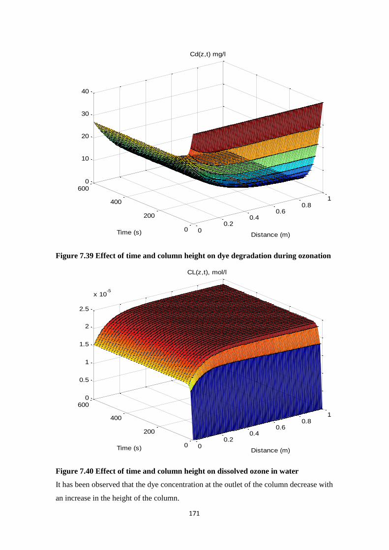
171
Figure 7.39 Effect of time and column height on dye degradation during ozonation
Figure 7.40 Effect of time and column height on dissolved ozone in water
It has been observed that the dye concentration at the outlet of the column decrease with
an increase in the height of the column.
00.2
0.40.6
0.81
0
200
400
6000
10
20
30
40
Distance (m)
Cd(z,t) mg/l
Time (s)
00.2
0.40.6
0.81
0
200
400
6000
0.5
1
1.5
2
2.5
x 10-5
Distance (m)
CL(z,t), mol/l
Time (s)
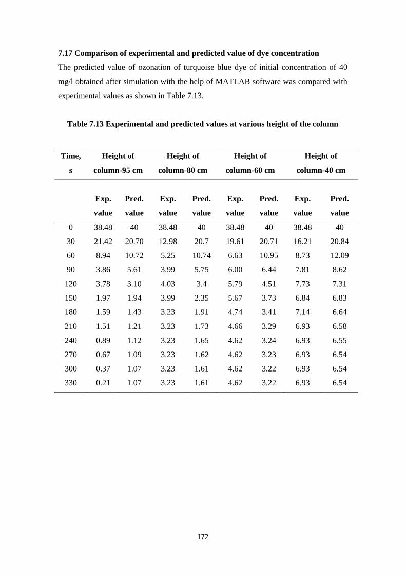
172
7.17 Comparison of experimental and predicted value of dye concentration
The predicted value of ozonation of turquoise blue dye of initial concentration of 40
mg/l obtained after simulation with the help of MATLAB software was compared with
experimental values as shown in Table 7.13.
Table 7.13 Experimental and predicted values at various height of the column
Time,
s
Height of
column-95 cm
Height of
column-80 cm
Height of
column-60 cm
Height of
column-40 cm
Exp.
value
Pred.
value
Exp.
value
Pred.
value
Exp.
value
Pred.
value
Exp.
value
Pred.
value
0 38.48 40 38.48 40 38.48 40 38.48 40
30 21.42 20.70 12.98 20.7 19.61 20.71 16.21 20.84
60 8.94 10.72 5.25 10.74 6.63 10.95 8.73 12.09
90 3.86 5.61 3.99 5.75 6.00 6.44 7.81 8.62
120 3.78 3.10 4.03 3.4 5.79 4.51 7.73 7.31
150 1.97 1.94 3.99 2.35 5.67 3.73 6.84 6.83
180 1.59 1.43 3.23 1.91 4.74 3.41 7.14 6.64
210 1.51 1.21 3.23 1.73 4.66 3.29 6.93 6.58
240 0.89 1.12 3.23 1.65 4.62 3.24 6.93 6.55
270 0.67 1.09 3.23 1.62 4.62 3.23 6.93 6.54
300 0.37 1.07 3.23 1.61 4.62 3.22 6.93 6.54
330 0.21 1.07 3.23 1.61 4.62 3.22 6.93 6.54
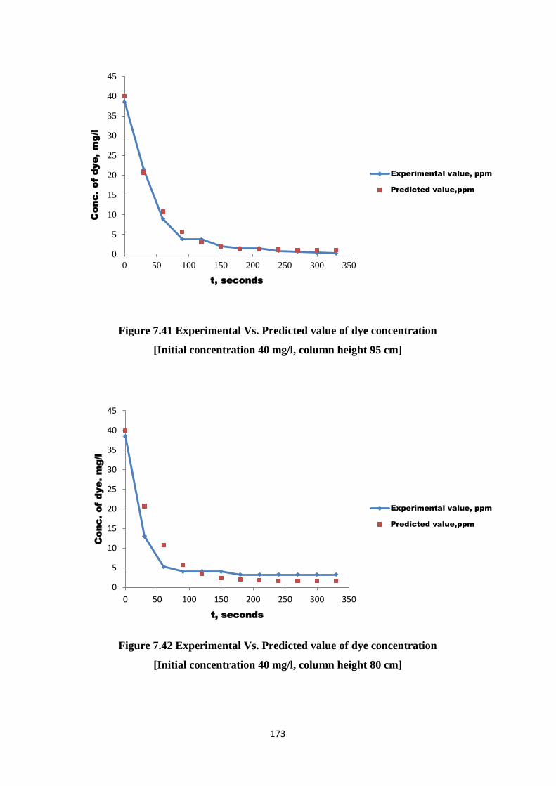
173
Figure 7.41 Experimental Vs. Predicted value of dye concentration
[Initial concentration 40 mg/l, column height 95 cm]
Figure 7.42 Experimental Vs. Predicted value of dye concentration
[Initial concentration 40 mg/l, column height 80 cm]
0
5
10
15
20
25
30
35
40
45
0 50 100 150 200 250 300 350
Conc. of dye, m
g/l
t, seconds
Experimental value, ppm
Predicted value,ppm
0
5
10
15
20
25
30
35
40
45
0 50 100 150 200 250 300 350
Conc. of dye. m
g/l
t, seconds
Experimental value, ppm
Predicted value,ppm
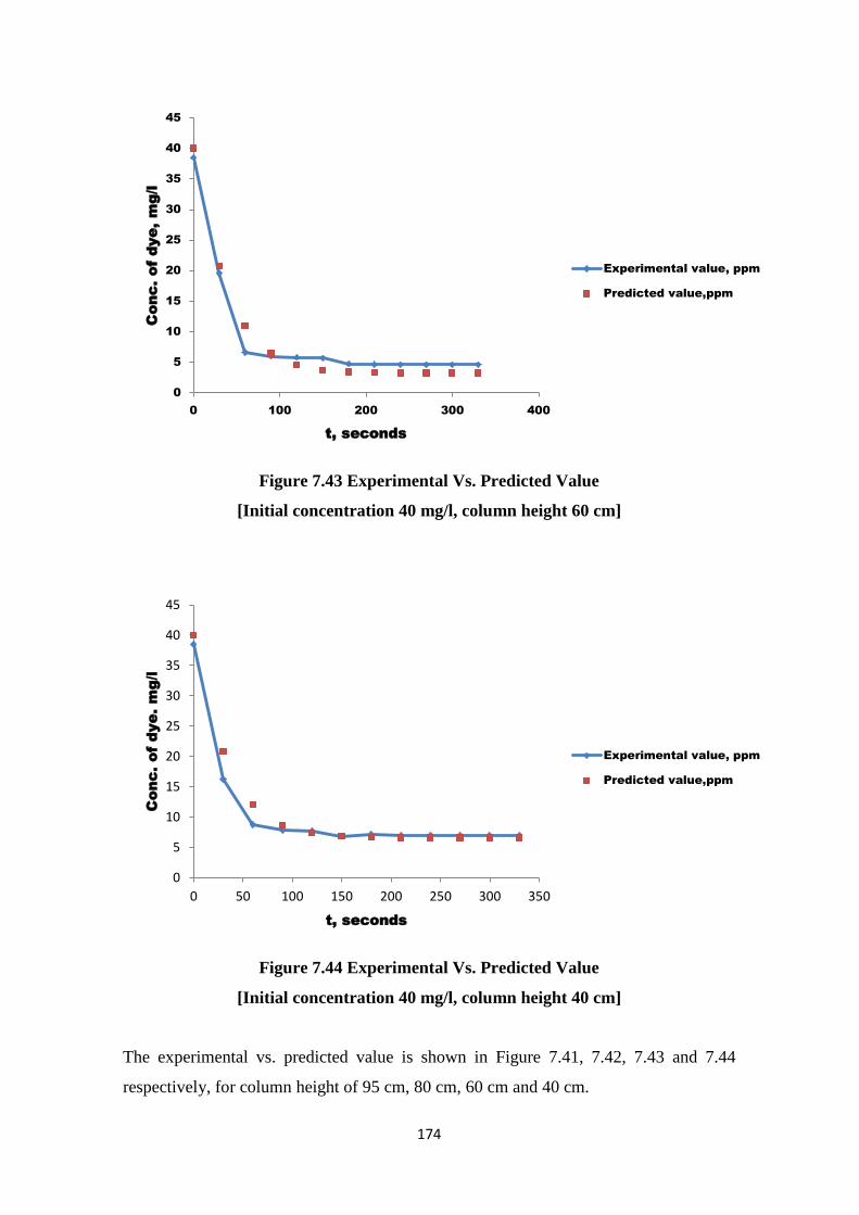
174
Figure 7.43 Experimental Vs. Predicted Value
[Initial concentration 40 mg/l, column height 60 cm]
Figure 7.44 Experimental Vs. Predicted Value
[Initial concentration 40 mg/l, column height 40 cm]
The experimental vs. predicted value is shown in Figure 7.41, 7.42, 7.43 and 7.44
respectively, for column height of 95 cm, 80 cm, 60 cm and 40 cm.
0
5
10
15
20
25
30
35
40
45
0 100 200 300 400
Conc. of dye, m
g/l
t, seconds
Experimental value, ppm
Predicted value,ppm
0
5
10
15
20
25
30
35
40
45
0 50 100 150 200 250 300 350
Conc. of dye. m
g/l
t, seconds
Experimental value, ppm
Predicted value,ppm
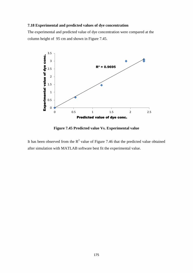
175
7.18 Experimental and predicted values of dye concentration
The experimental and predicted value of dye concentration were compared at the
column height of 95 cm and shown in Figure 7.45.
Figure 7.45 Predicted value Vs. Experimental value
It has been observed from the R2 value of Figure 7.46 that the predicted value obtained
after simulation with MATLAB software best fit the experimental value.
R² = 0.9695
0
0.5
1
1.5
2
2.5
3
3.5
0 0.5 1 1.5 2 2.5
Experim
enta
l value of dye conc.
Predicted value of dye conc.
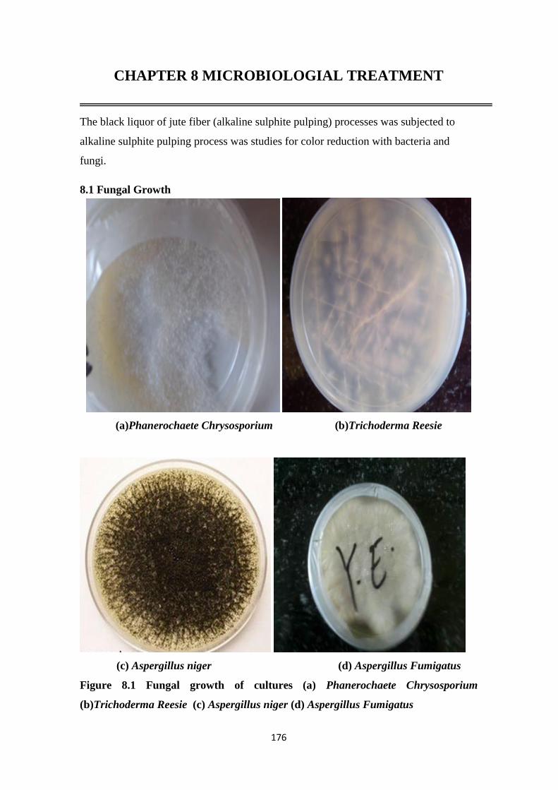
176
CHAPTER 8 MICROBIOLOGIAL TREATMENT
The black liquor of jute fiber (alkaline sulphite pulping) processes was subjected to
alkaline sulphite pulping process was studies for color reduction with bacteria and
fungi.
8.1 Fungal Growth
(a)Phanerochaete Chrysosporium (b)Trichoderma Reesie
(c) Aspergillus niger (d) Aspergillus Fumigatus
Figure 8.1 Fungal growth of cultures (a) Phanerochaete Chrysosporium
(b)Trichoderma Reesie (c) Aspergillus niger (d) Aspergillus Fumigatus
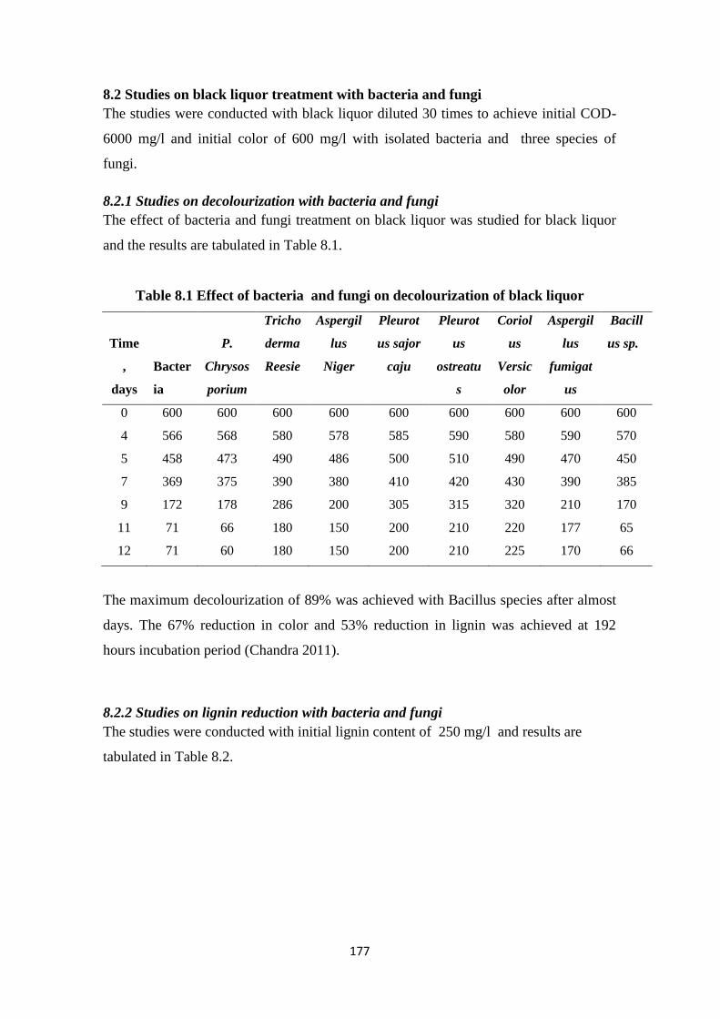
177
8.2 Studies on black liquor treatment with bacteria and fungi
The studies were conducted with black liquor diluted 30 times to achieve initial COD-
6000 mg/l and initial color of 600 mg/l with isolated bacteria and three species of
fungi.
8.2.1 Studies on decolourization with bacteria and fungi
The effect of bacteria and fungi treatment on black liquor was studied for black liquor
and the results are tabulated in Table 8.1.
Table 8.1 Effect of bacteria and fungi on decolourization of black liquor
Time
,
days
Bacter
ia
P.
Chrysos
porium
Tricho
derma
Reesie
Aspergil
lus
Niger
Pleurot
us sajor
caju
Pleurot
us
ostreatu
s
Coriol
us
Versic
olor
Aspergil
lus
fumigat
us
Bacill
us sp. A
0 600 600 600 600 600 600 600 600 600
4 566 568 580 578 585 590 580 590 570
5 458 473 490 486 500 510 490 470 450
7 369 375 390 380 410 420 430 390 385
9 172 178 286 200 305 315 320 210 170
11 71 66 180 150 200 210 220 177 65
12 71 60 180 150 200 210 225 170 66
The maximum decolourization of 89% was achieved with Bacillus species after almost
days. The 67% reduction in color and 53% reduction in lignin was achieved at 192
hours incubation period (Chandra 2011).
8.2.2 Studies on lignin reduction with bacteria and fungi
The studies were conducted with initial lignin content of 250 mg/l and results are
tabulated in Table 8.2.
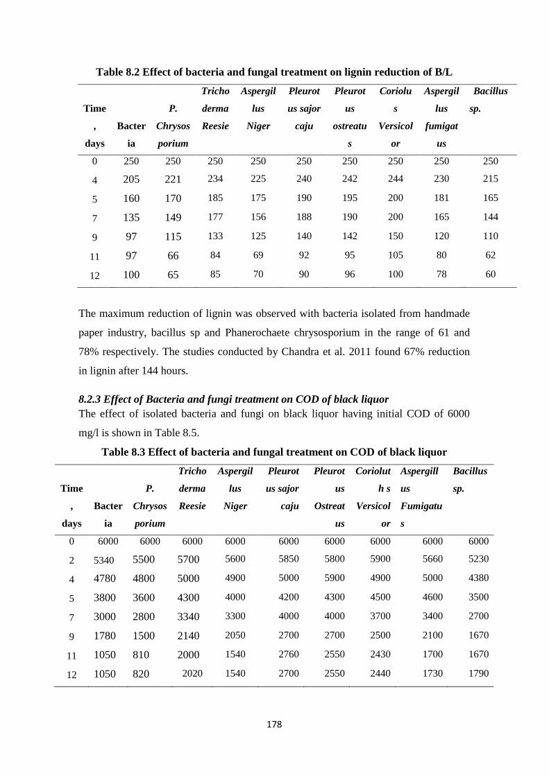
178
Table 8.2 Effect of bacteria and fungal treatment on lignin reduction of B/L
Time
,
days
Bacter
ia
P.
Chrysos
porium
Tricho
derma
Reesie
Aspergil
lus
Niger
Pleurot
us sajor
caju
Pleurot
us
ostreatu
s
Coriolu
s
Versicol
or
Aspergil
lus
fumigat
us
Bacillus
sp. A
0 250 250 250 250 250 250 250 250 250
4 205 221 234 225 240 242 244 230 215
5 160 170 185 175 190 195 200 181 165
7 135 149 177 156 188 190 200 165 144
9 97 115 133 125 140 142 150 120 110
11 97 66 84 69 92 95 105 80 62
12 100 65 85 70 90 96 100 78 60
The maximum reduction of lignin was observed with bacteria isolated from handmade
paper industry, bacillus sp and Phanerochaete chrysosporium in the range of 61 and
78% respectively. The studies conducted by Chandra et al. 2011 found 67% reduction
in lignin after 144 hours.
8.2.3 Effect of Bacteria and fungi treatment on COD of black liquor
The effect of isolated bacteria and fungi on black liquor having initial COD of 6000
mg/l is shown in Table 8.5.
Table 8.3 Effect of bacteria and fungal treatment on COD of black liquor
Time
,
days
Bacter
ia
P.
Chrysos
porium
Tricho
derma
Reesie
Aspergil
lus
Niger
Pleurot
us sajor
caju
Pleurot
us
Ostreat
us
Coriolut
h s
Versicol
or
Aspergill
us
Fumigatu
s
Bacillus
sp. A
0 6000 6000 6000 6000 6000 6000 6000 6000 6000
2 5340 5500 5700 5600 5850 5800 5900 5660 5230
4 4780 4800 5000 4900 5000 5900 4900 5000 4380
5 3800 3600 4300 4000 4200 4300 4500 4600 3500
7 3000 2800 3340 3300 4000 4000 3700 3400 2700
9 1780 1500 2140 2050 2700 2700 2500 2100 1670
11 1050 810 2000 1540 2760 2550 2430 1700 1670
12 1050 820 2020 1540 2700 2550 2440 1730 1790
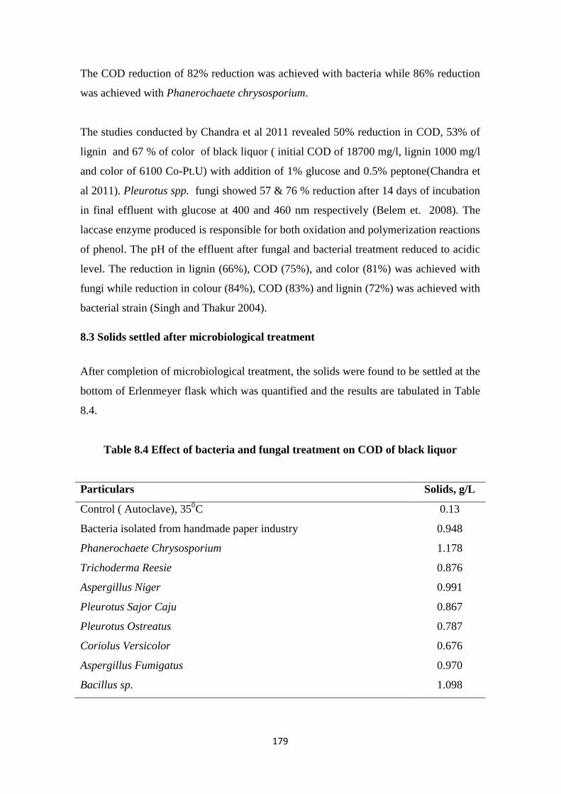
179
The COD reduction of 82% reduction was achieved with bacteria while 86% reduction
was achieved with Phanerochaete chrysosporium.
The studies conducted by Chandra et al 2011 revealed 50% reduction in COD, 53% of
lignin and 67 % of color of black liquor ( initial COD of 18700 mg/l, lignin 1000 mg/l
and color of 6100 Co-Pt.U) with addition of 1% glucose and 0.5% peptone(Chandra et
al 2011). Pleurotus spp. fungi showed 57 & 76 % reduction after 14 days of incubation
in final effluent with glucose at 400 and 460 nm respectively (Belem et. 2008). The
laccase enzyme produced is responsible for both oxidation and polymerization reactions
of phenol. The pH of the effluent after fungal and bacterial treatment reduced to acidic
level. The reduction in lignin (66%), COD (75%), and color (81%) was achieved with
fungi while reduction in colour (84%), COD (83%) and lignin (72%) was achieved with
bacterial strain (Singh and Thakur 2004).
8.3 Solids settled after microbiological treatment
After completion of microbiological treatment, the solids were found to be settled at the
bottom of Erlenmeyer flask which was quantified and the results are tabulated in Table
8.4.
Table 8.4 Effect of bacteria and fungal treatment on COD of black liquor
Particulars Solids, g/L
Control ( Autoclave), 350C 0.13
Bacteria isolated from handmade paper industry 0.948
Phanerochaete Chrysosporium 1.178
Trichoderma Reesie 0.876
Aspergillus Niger 0.991
Pleurotus Sajor Caju 0.867
Pleurotus Ostreatus 0.787
Coriolus Versicolor 0.676
Aspergillus Fumigatus 0.970
Bacillus sp. 1.098
180
There is maximum settled solids in Phanerochaete Chrysosporium with sequence of
settled solids (PC˃Bacillus sp> Aspergillus Niger˃ Bacteria from handmade
paper>Aspergillus Fumigatus>Pleurotus Sajor Caju>Pleurotus Ostreatus>Coriolus
Versicolor>and least in bacteria with 4 gpl glucose in aerobic conditions.
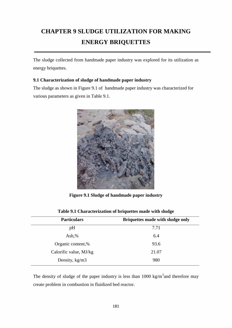
181
CHAPTER 9 SLUDGE UTILIZATION FOR MAKING
ENERGY BRIQUETTES
The sludge collected from handmade paper industry was explored for its utilization as
energy briquettes.
9.1 Characterization of sludge of handmade paper industry
The sludge as shown in Figure 9.1 of handmade paper industry was characterized for
various parameters as given in Table 9.1.
Figure 9.1 Sludge of handmade paper industry
Table 9.1 Characterization of briquettes made with sludge
Particulars Briquettes made with sludge only
pH 7.71
Ash,% 6.4
Organic content,% 93.6
Calorific value, MJ/kg 21.07
Density, kg/m3 980
The density of sludge of the paper industry is less than 1000 kg/m3and therefore may
create problem in combustion in fluidized bed reactor.
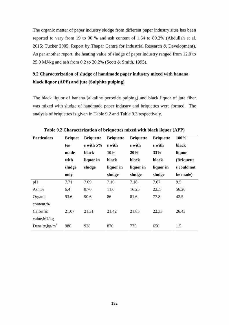
182
The organic matter of paper industry sludge from different paper industry sites has been
reported to vary from 19 to 90 % and ash content of 1.64 to 80.2% (Abdullah et al.
2015; Tucker 2005, Report by Thapar Centre for Industrial Research & Development).
As per another report, the heating value of sludge of paper industry ranged from 12.0 to
25.0 MJ/kg and ash from 0.2 to 20.2% (Scott & Smith, 1995).
9.2 Characterization of sludge of handmade paper industry mixed with banana
black liquor (APP) and jute (Sulphite pulping)
The black liquor of banana (alkaline peroxide pulping) and black liquor of jute fiber
was mixed with sludge of handmade paper industry and briquettes were formed. The
analysis of briquettes is given in Table 9.2 and Table 9.3 respectively.
Table 9.2 Characterization of briquettes mixed with black liquor (APP)
Particulars Briquet
tes
made
with
sludge
only
Briquette
s with 5%
black
liquor in
sludge
Briquette
s with
10%
black
liquor in
sludge
Briquette
s with
20%
black
liquor in
sludge
Briquette
s with
33%
black
liquor in
sludge
100%
black
liquor
(Briquette
s could not
be made)
pH 7.71 7.09 7.10 7.18 7.67 9.5
Ash,% 6.4 8.70 11.0 16.25 22..5 56.26
Organic
content,%
93.6 90.6 86 81.6 77.8 42.5
Calorific
value,MJ/kg
21.07 21.31 21.42 21.85 22.33 26.43
Density,kg/m3 980 928 870 775 650 1.5
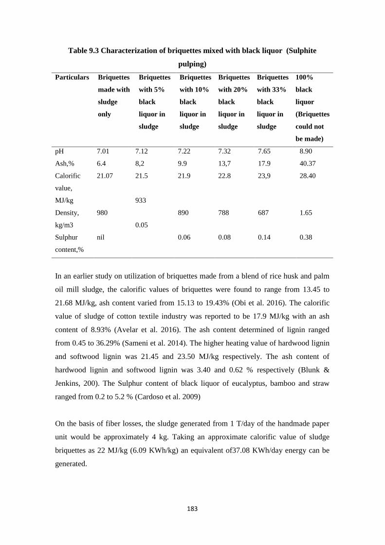
183
Table 9.3 Characterization of briquettes mixed with black liquor (Sulphite
pulping)
Particulars Briquettes
made with
sludge
only
Briquettes
with 5%
black
liquor in
sludge
Briquettes
with 10%
black
liquor in
sludge
Briquettes
with 20%
black
liquor in
sludge
Briquettes
with 33%
black
liquor in
sludge
100%
black
liquor
(Briquettes
could not
be made)
pH 7.01 7.12
8,2
21.5
933
0.05
7.22 7.32 7.65 8.90
Ash,% 6.4 9.9 13,7 17.9 40.37
Calorific
value,
MJ/kg
21.07 21.9 22.8 23,9 28.40
Density,
kg/m3
Sulphur
content,%
980
nil
890
0.06
788
0.08
687
0.14
1.65
0.38
In an earlier study on utilization of briquettes made from a blend of rice husk and palm
oil mill sludge, the calorific values of briquettes were found to range from 13.45 to
21.68 MJ/kg, ash content varied from 15.13 to 19.43% (Obi et al. 2016). The calorific
value of sludge of cotton textile industry was reported to be 17.9 MJ/kg with an ash
content of 8.93% (Avelar et al. 2016). The ash content determined of lignin ranged
from 0.45 to 36.29% (Sameni et al. 2014). The higher heating value of hardwood lignin
and softwood lignin was 21.45 and 23.50 MJ/kg respectively. The ash content of
hardwood lignin and softwood lignin was 3.40 and 0.62 % respectively (Blunk &
Jenkins, 200). The Sulphur content of black liquor of eucalyptus, bamboo and straw
ranged from 0.2 to 5.2 % (Cardoso et al. 2009)
On the basis of fiber losses, the sludge generated from 1 T/day of the handmade paper
unit would be approximately 4 kg. Taking an approximate calorific value of sludge
briquettes as 22 MJ/kg (6.09 KWh/kg) an equivalent of37.08 KWh/day energy can be
generated.
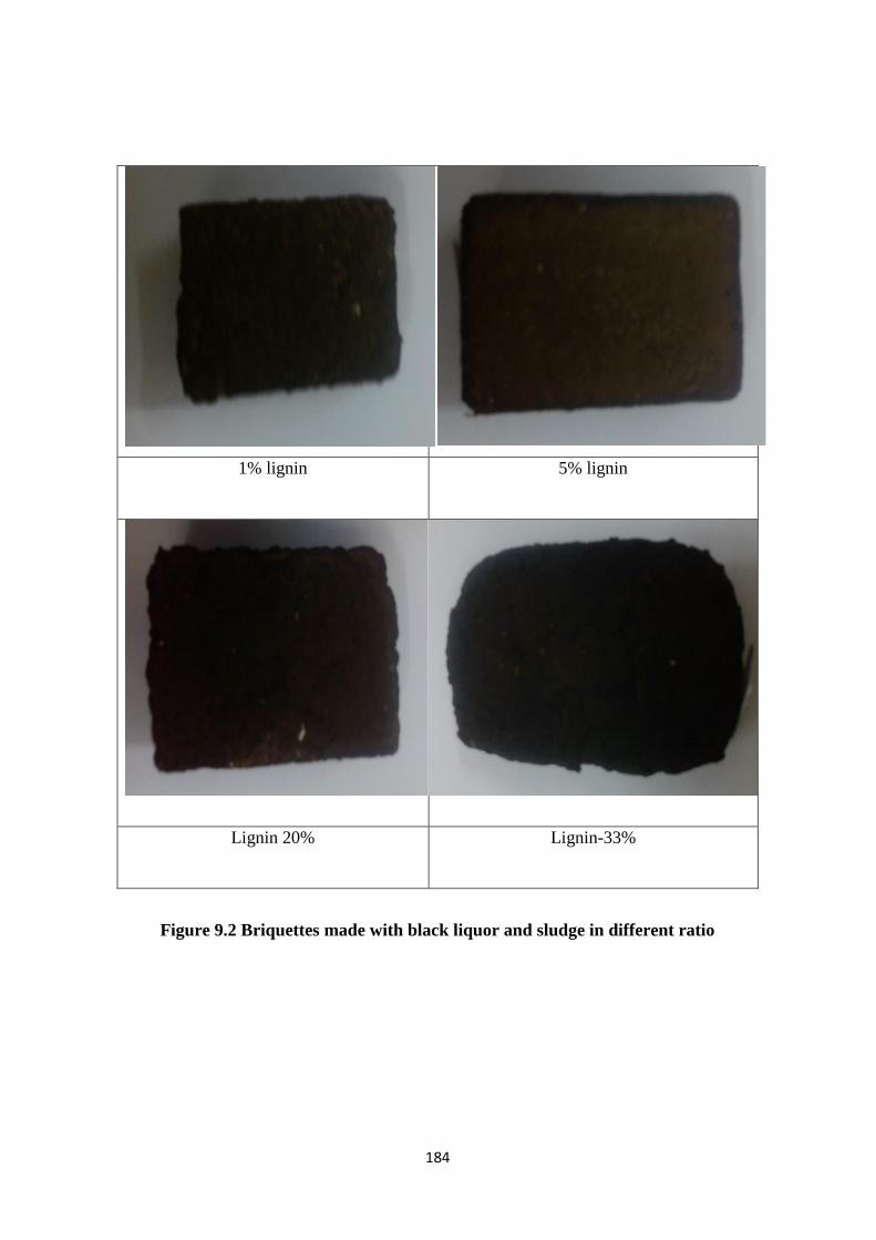
184
1% lignin
5% lignin
Lignin 20%
Lignin-33%
Figure 9.2 Briquettes made with black liquor and sludge in different ratio
185
CHAPTER 10 CONCLUSIONS & RECOMMENDATIONS
FOR FUTURE WORK
10.1 Conclusions
There is a cluster of more than 30 handmade paper units in Sanganer, Jaipur.
The wastewater discharged from these units exceeds the limits prescribed by the
Central Pollution Control Board; however, the effluent of handmade paper is
less polluted in comparison to paper mills. The handmade paper units utilize
cotton rags as conventional raw material. Some of the handmade paper units
utilize alternative ligno-cellulosic raw material like jute, Sunn hemp and Banana
fiber for handmade paper making. The black liquor contributes to major
pollution load. Direct dyes constitute the main colour producing component of
waste water discharge from the units contributing another major pollution load.
The Fly ash as low cost adsorbent has been proven as a potential adsorbent for
wastewater treatment of handmade paper industries. Batch studies have been
conducted on direct black dye synthetic wastewater using fly ash of specific
surface area 240 m2/g to derive adsorption isotherms. A comparison of R
2
values in isotherms studies showed best fitting for Langmuir isotherm. The
maximum adsorption capacity of fly ash was 76.33 mg/g at 318 K in batch
studies. The adsorption followed first order kinetics. The negative value of ∆G0
confirmed the feasibility of the process and spontaneous nature of adsorption of
fly ash.
The Yoon Nelson and Thomas models were found to have better fitting with
experimental data in fixed bed adsorption studies among the three models
employed to explain the behavior of the reactor. The numerical model
developed with the help of MATLAB showed excellent fitting with the
experimental values.
186
The results of COD, Color and BOD values of treated effluent with fly ash were
within prescribed norms of CPCB confirming that low cost fly ash is a potential
adsorbent to treat effluent of handmade paper industry containing black dye.
The adsorbed fly ash in a dosage of 5% was further utilized as additive in paper
making, which showed no adverse effect on strength properties of handmade
paper. From the cost analysis, fly ash has proven as a cheap alternative for
treatment of waste water compared to traditional adsorbents. The major
contribution lies in utilization of low cost fly ash in closed loop system.
Ozonation of synthetic samples of direct blue and red dyes was carried out in
column reactors in a controlled range of operating parameters like pH,
temperature and contact time in order to derive reaction kinetics. The study
showed that decolourization time varied from 12 to 4 minutes for blue dye with
removal increasing from 59.5% to 99% at pH of 4; the corresponding values
were 12 to 6 minutes and removal efficiency increase of 73% to 99% at pH 10
respectively for the red dye at an effluent temperature of 313 K. The equilibrium
time of decolourization with ozonation treatment for direct red and direct blue
dye for 50 mg/l initial concentration was 6 and 4 minutes, respectively. The
maximum COD removal of 45 and 54% was achieved for direct blue dye and
direct red dye solutions, respectively. The decolourization of dye solutions to
ozone followed the pseudo-first-order reaction with the maximum rate constant
for direct red and direct blue dyes as 0.917 and 0.904 min–1
respectively, at pH
of 10 and temperature of 313 K.
The ozonation treatment showed increase in decolourization efficiency of ozone
at high pH in case of both blue and red dye. The decolourization of dye
solutions with ozone is pseudo first order reaction with a maximum rate constant
achieved at pH-10. The maximum rate constant for direct red and direct blue
dye at pH-10 is 0.917 and 0.904 min-1
, respectively. The predicted values
achieved with the help of MATLAB software showed good fitting with
experimental values.
187
The black liquor of Jute fiber with sulphite pulping process having initial COD
of 6000 mg/l showed the maximum decolourization of 86% with the
Phanerochaete chrysosporium fungi.
The energy briquettes made by utilizing sludge of handmade paper industry
(solid fibers) and black liquor (liquid waste) showed calorific value above 20
MJ/kg indicating a potential reuse of the waste and closing the treatment loop.
Thus, from both the treatment processes, adsorption or ozone oxidation, the
sludge produced may be either reused for paper making (if the hue permits) or
be converted to energy briquettes thereby establishing a close loop cycle, which
can be practiced at the level of small scale units.
Therefore, it can be concluded that ozonation and adsorption are potential
treatment technologies for wastewater of handmade paper industry. The
ozonation treatment requires initial investment but with less operational cost.
The bacteria and fungi can be used in sequence with other treatment methods.
The ozonation treatment can be applied after adsorption and before
microbiological treatment to take care of only residual dyes for achieving
economy. The sludge of handmade paper industry along with black liquor can
be well used for making energy briquettes. Thus, the studies conducted on
wastewater of handmade paper industry using simple and cost effective
technologies can help improve the sustainability of the handmade paper
industry.
10.2 Recommendations for future work
The recommendations for the future work are as given below:
The surface charge of the dyes were not determined in the current work,
however it is recommended for future work.
Ozonation treatment may be studied for mixture of dyes.
188
REFERENCES
A report on opportunities for green chemistry initiatives: Pulp and Paper Industry, 2014,
Office of the Principal Scientific Advisor to GOI.
Aadil, K. R., Barapatre, A., and Jha, H. (2016). “Synthesis and characterization of
Acacia lignin-gelatin film for its possible application in food packaging”, Bioresources
and Bioprocessing, 3(1), 1-11.
Abdullah, R., Ishak, C. F., Kadir, W. R., and Bakar, R. A. (2015). “Characterization and
feasibility assessment of recycled paper mill sludges for land application in relation to
the environment”, International Journal of Environmental Research and Public Health,
12(8), 9314–9329.
Acemiog˘ lu, B. (2004). “Adsorption of Congo red from aqueous solution onto calcium-
rich fly ash”, Journal of Colloid and Interface Science, 274, 371–379.
Adamson, A. W., and Gast, A. P. (1997). “Physical Chemistry of Surfaces”, 6th
ed.
Wiley Interscience, New York.
Agarwal, S., Singh, K., Gupta, A. B., and Sharma, A. K. (2016). “Fly ash as low cost
adsorbent for treatment of effluent of handmade paper industry-Kinetic and modelling
studies for direct black dye”, Journal of Cleaner Production, 112, 1227–1240.
Aken, P. V., Broeck, R. V. D., Degrève, J., and Dewil, R. (2015). “The effect of
ozonation on toxicity and biodegradability of 2,4-dichlorophenol containing
wastewater”, Chemical Engineering Journal,
http://dx.doi.org/10.1016/j.cej.2015.06.019 (Accepted Manuscript).
Alluri, V. R. G. R., Rama, Sungnanam, S. D. P., Kunjam, M., and Nethala, V. K.
(2016). “Analysis of effluents released from the paper industry : Approach of its impact
on agricultural soil”, International Journal of Applied Research, 2 (7), 890–892.
189
APHA. (1989). “Standard Methods for the Examination of Water and Wastewater.”,
20th Edition. American Public Health Association, American Water Work Association,
Water Environment Federation, Washington, D.C.
Arslan-Alaton, I. (2003). “The effect of pre-ozonation on the biocompatibility of
reactive dye hydrolysates” Chemosphere, 51, 825–833.
Assalin, M. R., Almeida, E. S., Rosa, M. A., Moraes, S. G., and Duran, N. (2004).
“Application of Ozonation Process In Industrial Wastewaters: Textile, Kraft E1 and
Whey Effluents”, Environmental Technology, 25(8), 867–872.
ASTM E-1131-08, 2012, Standard Test method for compositional analysis by
Thermogravimetry.
Auta, M., and Hameed, B.H. (2012). “Modified mesoporous clay adsorbent for
adsorption isotherm and kinetics of methylene blue”, Chemical Engineering Journal,
198-199, 219–227.
Aharoni, C., Sideman, S., and Hoffer, E. (1979). “Adsorption of phosphate ions by
colloid ion coated alumina”, Journal of Chemical Technology and Biotechnology, 29,
404–412.
Aharoni, C., and Ungarish, M. (1977). Kinetics of activated chemisorption Part 2.
Theoretical
Models”, Journal of the Chemical Society Faraday Transactions, 73, 456-464.
Bajpai, P., and Bajpai, P. K., (1994). “Biological colour removal of pulp and paper mill
wastewaters.” Journal of Biotechnology, 33, 211-220.
Bajpai., P. (2016). “Global Pulp and Paper Production and Consumption.”, Pulp and
Paper Industry: Energy conservation, 9-14.
Bajeer, M. A., Nizamani, S. M., Hussainsherazi, S. T., and Bhanger, M. I. (2012).
Adsorption and leaching potential of imidacloprid pesticide through alluvial soil”,
American Journal of Analytical Chemistry, 3, 604-611.
190
Barapatre, A., and Jha, H. (2016). “Decolourization and Biological Treatment of Pulp
and Paper Mill Effluent by Lignin-Degrading Fungus Aspergillus flavus Strain F10 5”,
International Journal of Current Microbiology and Applied Sciences, 5(5), 19–32.
Belém, A., Panteleitchouk, A. V., Duarte, A. C., Rocha-Santos, T. A. P., and Freitas, A.
C. (2008). “Treatment of the effluent from a kraft bleach plant with white rot fungi
Pleurotus sajorcaju and Pleurotus ostreatus”, Global Nest Journal, 10(3), 426–431.
Beltrán, F. J., González, M., Acedo, B., and Rivas, F. J. (2000). “Kinetic modelling of
aqueous atrazine ozonation processes in a continuous flow bubble contactor”, Journal
of Hazardous Materials, 80, 189–206.
Beltrán, F. J., Aguinaco, A., and García-araya, J. F. (2010). “Kinetic modelling of TOC
removal in the photocatalytic ozonation of diclofenac aqueous solutions”, Applied
Catalysis B : Environmental, 100, 289–298.
Biermann, C. 2012, Handbook of Pulping and Papermaking, 2nd
Edition, 1-754.
Biń, A. K., Duczmal, B., and Machniewski, P. (2001). “Hydrodynamics and ozone
mass transfer in a tall bubble column”, Chemical Engineering Science, 56, 6233–6240.
Blunk, S. L. and Jenkins, B. M. (2000), “Combustion properties of lignin residue from
ligno-cellulose fermentation.”, 1-15.
Boeriu, C. G., Bravo, D., Gosselink, R. J. A., and Van Dam, J. E. G. (2004).
“Characterisation of structure-dependent functional properties of lignin with infrared
spectroscopy”, Industrial Crops and Products, 20, 205–218.
Boruah , P., Dowarah, P., Hazarika, R., Yadav, A., Barkakati, P., and Goswami, T.
(2016). “Xylanase from Penicillium meleagrinum var. viridiflavum - a potential source
for bamboo pulp bleaching”, Journal of Cleaner Production. doi:
10.1016/j.jclepro.2015.12.024 (Accepted manuscript).
Brebu, M., and Vasile, C. (2010). “Thermal degradation of lignin- A review”, Cellulose
Chemistry and Technology, 44, 353–363.
191
Cardoso, M., de Oliveira, É. D., and Passos, M. L. (2009). “Chemical composition and
physical properties of black liquors and their effects on liquor recovery operation in
Brazilian pulp mills”, Fuel, 88(4), 756–763.
Casey, J. P. (1980). “ Pulp and Paper: Chemistry and Chemical Technology.”, Third
edition, 2, 1-576.
Central Pollution Control Board. (2006). “Development of guidelines for water
conservation in pulp and paper sector”, National Productivity Council, New Delhi.
Chandra, R., Abhishek, A., and Sankhwar, M. (2011). “Bacterial decolorization and
detoxification of black liquor from rayon grade pulp manufacturing paper industry and
detection of their metabolic products”, Bioresource Technology, 102, 6429-6436.
Chandra, R., and Abhishek, A. (2011). “Bacterial decolorization of black liquor in
axenic and mixed condition and characterization of metabolites”, Biodegradation, 22,
603–611.
Central Pollution Control Board. (2015). “Charter for Water Recycling and Pollution
Prevention in Pulp and Paper Industries (Specific to Ganga River Basin States)”,
Charter of paper industry, Annexure-I.
Chakradhar, B., and Shrivastava, S. (2004). “Colour removal of pulp and paper
effluents”, Indian Journal of Chemical Technology 11, 617–621.
Chatterjee, A. K. (2010). “Indian fly Ashes, their characteristics, and potential for
mechano-chemical activation for enhanced usability”, In: IInd International
Conference on Sustainable Construction Material and Technologies.
Chaudhari, P. K., Majumdar, B., Choudhary, R., Yadav, D. K., and Chand, S. (2010).
“Treatment of paper and pulp mill effluent by coagulation”, Environmental
Technology, 31, 357–363.
Chavan, S. K., and Paul, S. A. (2013). “Waste coal fly ash utilized for removal of
sulphur dye
192
from textile waste water: kinetics and equilibrium study”, Journal of Chemical,
Biological and Physical Sciences, 3, 1727-1734.
Chen, H. L., Chen, Y. C., Zhan, H. Y., and Fu, S. Y. (2010). “Enhanced Biodegradation
of Pulping Effluents By a Statistical Experimental Design Using Microbial Consortia”,
Bioresources, 5, 1581–1594.
Chen, Y. H., Chang, C. Y., Chiu, C. Y., Yu, Y. H., Chiang, P. C., Ku, Y., and Chen, J.
N. (2003). “Dynamic behavior of ozonation with pollutant in a counter current bubble
column with oxygen mass transfer”, Water Research, 37, 2583–2594.
Chongrak, K., Eric, H., Noureddine, A., and Jean, P. (1998). “Application of Methylene
Blue Adsorption to Fiber Specific Surface Area Measurement”, Journal of Cotton
Science, 2:164-173.
Ciardelli, G., and Ranieri, N. (2001). “Technical Note the Treatment and Reuse of
Wastewater in the Textile Industry By Means of Ozonation and Electroflocculation”,
Water Research, 35(2), 567–572.
Cibichakravarthy, G. V., Ramanathan, B., Nallapeta, A. S., Mula, and R. V. R., Rayalu,
J. (2012). “Decolourization of paper mill effluent by immobilized cells of
Phanerochaete Chrysosporium”, International Journal of Plant, Animal and
Environmental Sciences, 141–146.
Colindres, P., Yee-Madeira, H., and Reguera, E. (2010). “Removal of Reactive Black 5
from aqueous solution by ozone for water reuse in textile dye processes”, Desalination,
258, 154-158.
Cotana, F., Cavalaglio, G., Nicolini, A., Gelosia, M., Coccia, V., Petrozzi, A., and
Brinchi, L. (2014). “Lignin as co-product of second generation bioethanol production
from ligno-cellulosic biomass”, Energy Procedia, 45(0), 52–60.
Dangcong, P., and Qiting, J. (1993). “Anaerobic digestion of alkaline black liquor using
an upflow anaerobic sludge blanket reactor”, Journal of Chemical Technology
Biotechnology, 58, 89–93.
193
Daniels, W. L., Stewart, B., Haering, K., and Zipper, C. (2002). “The Potential for
beneficial Reuse of Coal Fly Ash in southwest virginia Mining environments”, Powell
River Project, Virginia Cooperative Extension, 460-134.
Dashtban, M., Schraft, H., Syed, T. A., and Qin, W. (2010). “Fungal biodegradation and
enzymatic modification of lignin”, International Journal Biochemistry Molecular
Biology, 1, 36–50.
Davy, M. F., Uloth, V.C., and Cloutier, J. N. (1998). “Economic evaluation of black
liquor treatment processes for incremental kraft pulp production”, Pulp & Paper
Canada, 99( 2), 35–39.
Devi, T. S. R., and Gayathri, S. (2010). “FTIR and FT-Raman spectral analysis of
paclitaxel drugs”, International Journal of Pharmaceutical Sciences Review and
Research, 19, 106-110.
Devi, N. L., Yadav, I. C., Shihua, Q. I., Singh, S., and Belagali, S. L. (2011).
“Physicochemical characteristics of paper industry effluents - A case study of South
India Paper Mill (SIPM).”, Environmental Monitoring and Assessment, 177, 23–33.
Dhadse, S., Kumari, P., and Bhagia, L. J.(2008). “Fly ash characterization, utilization
and government initiatives in India - A review.”, Journal of Scientific & Industrial
Research, 67, 11–18.
Dhanushree, M. S., and Kousar, H. (2015). “An Overview of certain Physico-chemical
Parameters of Paper Mill Effluent Department of Post Graduate Studies and Research in
Environmental Science , Kuvempu University , 4, 195–197.
Dhaouadi, H., Poncin, S., Hornut, J. M., and Midoux, N. (2008). “ Gas – liquid mass
transfer in bubble column reactor : Analytical solution and experimental confirmation.”,
Chemical Engineering & Processing, 47, 548–556.
Dogruel, S., Genceli, E. A., Babuna, F. G., and Orhon, D. (2006). “ An investigation on
the optimal location of ozonation within biological treatment for a tannery
wastewater.”, Journal of Chemical Technology and Biotechnology, 81, 1877–1885.
194
Dubinin, M. M. (1960). “The potential theory of adsorption of gases and vapours for
adsorbents with energetically nonuniform surfaces.”, Chemical Reviews, 60, 235–241.
El-Din, M. G., and Smith, D. W. (2003). “Mass transfer analysis in ozone bubble
columns.”, Journal of Environmental Engineering Science, 2, 63–76.
EPA Notifications’ 64(E), dated 18 Jan 1998; Environment Protection rules 1986
Erol, F., Özbelge, T. A., and Özbelge, H. Ö. (2009). “Modeling of catalytic ozonation
process in a three-phase reactor.”, Journal of Environmental Science and Health Part
A : Toxic / Hazardous Substances and Environmental Engineering, 44, 295-306.
Fanchiang, J. M., Tseng, and D. H. (2009). “ Degradation of anthraquinone dye C.I.
Reactive Blue 19 in aqueous solution by ozonation.”, Chemosphere 77, 214–221.
Faria, P. C. C., Orfao, J. J. M., Pereira, and M. F. R. (2009). “Activated carbon and
ceria catalysts applied to the catalytic ozonation of dyes and textile effluents.”, Applied
Catalysis B: Environmental, 88, 341–350.
Filipkowska, U., Klimiuk, E., Kuczajowska-Zadrożna, M., Kuś, S. (2004). “The
Removal of Reactive Dyes from Binary Mixtures Using Chitin.”, Polish Journal of
Environmental Studies, 13, 65-661.
Font, X., Caminal, G., Gabarrell, X., Romero, S., and Vicent, M. T. (2003). “Black
liquor detoxification by laccase of Trametes versicolour pellets.”, Journal of Chemical
Technology and Biotechnology, 78, 548–554.
Fracaro, G., Vakkilainen, E., Hamaguchi, M., De Souza, and S. N. M. (2012). “Energy
efficiency in the Brazilian pulp and paper industry.”, Energies 5, 3550–3572.
Freundlich, H. M.F. (1906). “Over the adsorption in solution.”, The Journal of Physical
Chemistry, 57,385-471.
Garg, V. K., Gupta, R., Kumar, R., and Gupta, R. K. (2004). “Adsorption of chromium
from aqueous solution on treated sawdust.”, Bioresources Technology, 92, 79–81.
195
Giri, K., Patel, R. K., and Mahapatra, S. S. (2011). “Artificial neural network (ANN)
approach for modeling of arsenic (III) biosorption from aqueous solution by living cells
of Bacillus cereus biomass.”, Chemical Engineering Journal, 178, 15-25.
Gomes, A. C., Fernandes, L. R. and Simões, R. M. S. (2012). “Oxidation rates of two
textile dyes by ozone: Effect of pH and competitive kinetics.”, Chemical Engineering
Journal, 189–190, 175–181.
Grover, R., Marwaha, S. S., and Kennedy, J. F. (1999). “Studies on the use of an
anaerobic baffled reactor for the continuous anaerobic digestion of pulp and paper mill
black liquors.”, Process Biochemistry, 34, 653–657.
Gong, X., Takagi, S., Huang, H., and Matsumoto, Y. (2007). “A numerical study of
mass transfer of ozone dissolution in bubble plumes with an Euler – Lagrange
method.”, Chemical Engineering Science, 62, 1081–1093.
Guendy, H. R. (2007). “Ozone treatment of textile wastewater relevant to toxic effect
elimination in marine environment.”, Egyptian Journal of Aquatic Research, 33, 98–
115.
Gupta, G., Prasad, G., Panday, K. K., and Singh, V. N. (1988). “Removal of chrome
dye from
aqueous solutions by fly ash.”, Water, Air & Soil Pollution, 37, 13-24.
Hameed, B. H., Ahmad, A. A., and Aziz, N. (2007). “Isotherms, kinetics and
thermodynamics of acid dye adsorption on activated palm ash.”, Chemical Engineering
Journal, 133(1–3), 195–203.
Han, R., Ding, D., Xu, Y., Zou, W., Wang, Y., Li, Y., and Zou, L. (2008). “Use of rice
husk for the adsorption of congo red from aqueous solution in column mode.”,
Bioresource Technology, 99(8), 2938–2946.
196
Han, Z.-X., Zhu, Z., Wu, D., Wu, J., and Liu, Y. (2014). “Adsorption Kinetics and
Thermodynamics of Acid Blue 25 and methylene blue dye solutions on natural
sepiolite.”, Synthesis and Reactivity in Inorganic, Metal-Organic and Nano-Metal
Chemistry, 44(1), 140–147.
Hariharan, S., and Nambisan, P. (2013). “Optimization of Lignin Peroxidase,
Manganese Peroxidase, and Lac Production from Ganoderma lucidum Under Solid
State Fermentation of Pineapple Leaf.”, Bioresources, 8(1), 250–271.
Hasan, S. H., and Srivastava, P. (2011). “Biosorptive Abatement of Cd 2 + by Water
Using Immobilized Biomass of Arthrobacter sp . : Response Surface Methodological
Approach.”, Industrial & Engineering Chemistry Research, 247–258.
He, S. H., Li, J., Xu, J., and Mo, L. (2016). “ Enhanced Removal of COD and Colour in
Paper-making Wastewater by Ozonation Catalyzed by Fe Supported on Activated
Carbon.”, Bioresources, 11 (4), 8396–8408.
Heidrich, C., Feuerborn, H., and Weir, A. (2013). Coal Combustion Products : a Global
Perspective. World of Coal Ash, 17.
Helmy, S. M., Rafie, S. E., and Ghaly, M. Y. (2003). “ Bioremediation post-photo-
oxidation and coagulation for black liquor effleunt treatment.”, Desalination, 158 , 331-
339.
Hoa, D. T. and Man, T. D. (2006). “ Study on treatment of alkaline black liquor using
sulphate reducing bacteria.”, Advances in Natural Sciences, 7(1), 139–145.
Hoigné, J., and Bader, H. (1983). “Rate constants of reactions of ozone with organic
and inorganic compounds in water-I. Non-dissociating organic compounds.”, Water
Research, 17, 173-183.
Ho, Y. S., and McKay, G. (1998). “Sorption of dye from aqueous solution by peat.”,
Chemical Engineering Journal, 70, 115–124.
Hu, Z., Que, Y., Gao, Y., Yin, Y., and Zhao, Y. (2015). “Using Black Liquor from the
Soda Pulping Process for Protein Production by Candida utilis.”, 10(3), 3908–3921.
197
ISO-11358-1:2014, Plastics-Thermogravimetry (TG) of polymers-Part I General
Principles
Irfan, M., Butt, T., Imtiaz, N., Abbas, N., Ahmad, R., and Shafique, A. (2013). “The
removal of COD, TSS and colour of black liquor by coagulation – flocculation process
at optimized pH, settling and dosing rate.”, Arabian Journal of Chemistry, 1-12.
Jaganathan, B., Hossain, S. K. M., Begum, K. M. M. S., and Anantharaman, N. (2009).
“Aerobic Pollution Abatement of Pulp mill Effluent with the White Rot fungus
Phanerochaete chrysosporium in Three-phase Fluidized Bed Bioreactor.”, Chemical
Engineering Research, 13, 13–16.
Jogarao. (2016). “How to recover more used paper for recycling.”, Indian Pulp and
Paper Technical Association, 28 (1), 84-87.
Kahraman, S., Dogan, N., and Erdemoglu, S. (2008). “Use of various agricultural
wastes for the removal of heavy metal ions, International Journal of Environment and
Pollution, 34, 275–284.
Kamali, M., Gameiro, T., Costa, M. E. V, and Capela, I. (2016). “Anaerobic digestion
of pulp and paper mill wastes - An overview of the developments and improvement
opportunities.”, Chemical Engineering Journal, 298, 162–182.
Kannan, N., and Sundaram, M. M. (2001). “Kinetics and mechanism of removal of
methylene blue by adsorption on various carbons—a comparative study.”, Dyes and
Pigments, 51, 25–40.
Kao, P. N., Tzeng, J. H., and Huang, T. L. (2000). “Removal of chlorophenols from
aqueoussolution by fly ash.”, Journal of Hazardous Materials, 76, 237-249.
Kara, S., Aydiner, C., Demirbas, E., Kobya, M., and Dizge, N. 2007). “Modeling the
effects of adsorbent dose and particle size on the adsorption of reactive textile dyes by
fly ash.”, Desalination, 212 (2007) 282–293.
198
Kavitha, D., and Namasivayam, C. (2007). “Experimental and kinetic studies on
methylene blue adsorption by coir pith carbon.”, Bioresources Technology, 98, 14–21.
Kesalkar, V. P., Khedikar, I. P., and Sudame, A. M. (2012). “Physico-chemical
characteristics of wastewater from Paper Industry.”, International Journal of
Engineering Research and Applications, 2 (4), 137–143.
Khan, T. A., Singh, V. V., and Kumar, D. (2004). Removal of some basic dyes from
artificial textile wastewater by adsorption on Akash Kinari coal. Journal of Scientific &
Industrial Research, 63, 355-364.
Khan, H., Ahmad, N., Yasar, A., and Shahid, R. (2010). “Advanced oxidative
decolorization of red Cl-5B:Effects of dye concentration, process optimization and
reaction kinetics.”, Polish Journal of Environmental Studies, 19(1), 83–92.
Khosla, E., Kaur, S., and Dave, P. N. (2013). “Tea waste as adsorbent for ionic dyes.”,
Desalination and Water Treatment, 51, 6552–6561.
Kirk, T. K., and Cullen, D. (1998). “Enzymology and molecular genetics of wood
degradation by white-rot fungi.” In: Young RA, Akhtar M (eds) Environmentally
friendly technologies for the pulp and paper industry. Wiley, New York, 273–307.
Ko, D.-S., Sauer, K., Nord, S., Müller, R., and Wolfrum, J. (1997). “Determination of
the diffusion coefficient of dye in solution at single molecule level.”, Chemical Physics
Letters, 269(1–2), 54–58.
Koch, M., Yediler, A., Lienert, D., Insel, G., and Kettrup, A. (2002). “Ozonation of
hydrolyzed azo dye reactive yellow 84 (CI).”, Chemosphere 46, 109–113.
Kolovea, E. P., The Use of Fly Ash for Lead Removal from Industrial Wastes, PhD
Dissertation, Aristotle University of Thessaloniki, Thessaloniki, Greece, 1982, 76–79.
Konsowa, A. H., Ossman, M. E., Chen, Y., and Crittenden, J. C. (2010).
“Decolourization of industrial wastewater by ozonation followed by adsorption on
activated carbon.” Journal of Hazardous Materials, 176, 181–185.
199
Kozakova, Z., Nejezchleb, M., Krcma, F., Halamova, I., Caslavsky, J., and Dolinova, J.
(2010). “Removal of organic dye direct red 79 from water solutions by DC diaphragm
discharge: Analysis of decomposition products.”, Desalination, 258, 93–99.
Kulshrestha, N. K. (1988). “Analysis of Financial Statements of Indian Paper
Industry.” Navman Prakashan, 1-2.
Kumar, V., Mathur, M., Sinha, S. S., and Dhatrak, S. (2005). “Fly Ash: an Environment
Savior.”, Fly Ash India. TIFAC, New Delhi. IVth 1.1-1.4.
Kumar, P., Teng, T. T., Chand, S., and Wasewar, K. L. (2011). “Treatment of Paper and
Pulp Mill Effluent by Coagulation.”, International Journal of Chemical, Molecular,
Nuclear, Materials and Metallurgical Engineering, 5(8), 715–720.
Kumar, A., Chaudhary, P., and Verma, P. (2013). “Adsorption of reactive red 194 dye
from textile effluent by using class F fly ash.”, Scholars Journal of Applied Medical
Sciences, 1, 111-116.
Kundu, S., and Gupta, A. K. (2006). “Arsenic adsorption onto iron oxide-coated cement
(IOCC): regression analysis of equilibrium data with several isotherm models and their
optimization.”, Chemical Engineering Journal, 122, 93-106.
Kuosa, M., Haario, H., and Kallas, J. (2006). “Axial Dispersion Model for Estimation
of Ozone Self- Decomposition Axial Dispersion Model for Estimation of Ozone Self-
Decomposition.”, Ozone : Science & Engineering : The Journal of the International
Ozone Association, 27, 409-417.
Kuosa, M., Laari, A., and Kallas, J. (2004). “Determination of the Henry’s coefficient
and mass transfer for ozone in a bubble column at different pH values of water.”,
Ozone: Science & Engineering, 26 (3), 277–286.
Kusvuran, E., Gulnaz, O., Samil, A., and Erbil, M. (2010). “Detection of double-bond
ozone stoichiometry by an iodimetric method during ozonation processes.”, Journal of
Hazardous Materials, 175, 410-416.
200
Kuzhali, S. S., Manikandan, N., and Kumuthakalavalli, R. (2012). “Physico chemical
and biological parameters of paper industry effluent.”, Journal of Natural Product and
Plant Resources, 2(3), 445–448.
Lafi, W. K., and Qodah, Z. A. (2006). “Combined advanced oxidation and biological
treatment processes for the removal of pesticides from aqueous solutions.”, Journal of
Hazardous Materials, 137 (2006) 489–497.
Lakdawala, M. M., and Oza, B. N.(2011). “Removal of BOD contributing components
from sugar Industry waste water using bagasse fly ash- waste material of sugar
Industry.”, Der Chemica Sinica, 2 (4), 244-251.
Langlais, B., Reckhow, D. A., and Brink, D. R. (1991). “Ozone in water treatment-
application and engineering.”, Lewis Publisher, American Water Works Association
Research Foundation, Michigan.
Lee, S. H., Kim, H. J., Sakai, E., and Daimon, M. (2003). “Effect of particle size
distribution of fly ash-cement system on the fluidity of cement pastes.”, Cement and
Concrete Research, 33, 763–768.
Li, H., Cao, X., Zhang, C., Qing, Y., Zhao, Z., Niu, X., Sun, X., Liu, Y., Ma, L., and Li, Z.
(2017). “Enhanced adsorptive removal of anionic and cationic dyes from single or mixed
dye solutions using MOF PCN-222.”, Royal Society of Chemistry Advances, 7, 16273-
16281.
Lin, S. H., and Lin, C. M. (1993). “Treatment of Textile Waste Effluents by Ozonation
and Chemical Coagulation.”, Water Research, 27 (12), 1743-1748.
Lin, S. Y. and Dence, C. W. (1992). “ Methods in lignin chemistry.”, Springer-Verlag,
1-568.
Lokeshappa, B., and Dikshit, A. K. (2011). “Disposal and management of fly ash.”,
Internation Conference on Life Science and Technology (IPCBEE). 3, Singapore.
201
Loutfi, H., Blackwell, B., and Uloth, V. (1991). “Lignin recovery from kraft black
liquor: Preliminary process design.” TAPPI Journal, 74(1), 203–210.
Lu, X., Yang, B., Chen, J., and Sun, R. (2009). “Treatment of waste water containing
azo dye reactive brilliant red X-3B using sequential ozonation and upflow biological
and aerated filter press.”, Journal of Hazardous Materials, 161, 241–245.
Mandavgane, S. A. and Yenkie, M. K. N. (2011). “Effect of pH on the medium on
degradation of aqueous ozone.”, Rasayan J Chem, 3, 544-547.
Marce, M., Domenjoud, B., Esplugas, S., and Baig, S. (2016). “Ozonation treatment of
urban primary and bio treated wastewaters : Impacts and modeling.”, Chemical
Engineering Journal, 283, 768–777.
Mall, I. D., Srivastava, V. C., and Agarwal, N. K. (2006). “Removal of Orange-G and
Methyl Violet dyes by adsorption onto bagasse fly ash - Kinetic study and equilibrium
isotherm analyses.”, Dyes and Pigments, 69, 210–223.
Maroto-Valer, M. M., Taulbee, D. N., and Hower, J. C. (2001). “Characterization of
differing forms of unburned carbon present in fly ash separated by density gradient
centrifugation.”, Fuel, 80, 795–800.
Mehmet, F. S., and Hasan, Z. S. (2002). “Ozone treatment of textile effluents and dyes:
Effect of applied ozone dose, pH and dye concentration.”, Journal of Chemical
Technology and Biotechnology, 77, 842–850.
Meric, S., Selcuk, H., and Belgiorno, V. (2005). “Acute toxicity removal in textile
finishing waste water by Fenton’s oxidation, ozone and coagulation–flocculation
processes.”, Water Research, 39, 1147–1153.
Meza, P. R., Felissia, F. E., and Area, M. C. (2010). “Reduction of the recalcitrant COD
of high yield pulp mills effluents by AOP. Part 1. Combination of ozone and activated
sludge.”, Bioresources, 6(2), 1053-1068.
202
Mittal, A., Jhare, D., and Mittal, J. (2013). “Adsorption of hazardous dye Eosin Yellow
from aqueous solution onto waste material De-oiled Soya: Isotherm, kinetics and bulk
removal.”, Journal of Molecular Liquids, 179, 133–140.
Mittal, A., and Lishakurup, M. J. (2007). “Freundlich and Langmuir adsorption
isotherms and kinetics for the removal of Tartrazine from aqueous solutions using hen
feathers.”, Journal of Hazardous Materials, 146, 243-248.
Mitani, M. M., Keller, A. A., Sandall, O. C., and Rinker, R. G. (2005). “Mass transfer
of ozone using a microporous diffuser reactor system.”, Ozone Science and
Engineering, 27, 45–51.
Nassar, M. (2003). “Thermal Behavior of Bagasse Kraft Black Liquor.”, Energy
Sources, 25(8), 837–844.
Negrão, D. R., Sain, M., Leão, A. L., Sameni, J., Jeng, R., De Jesus, J. P. F., and
Monteiro, R. T. R. (2015). “Fragmentation of lignin from organosolv black liquor by
white rot fungi.”, BioResources, 10(1), 1553–1573.
Nouri, H., and Ouederni, A. (2013). “Modeling of the Dynamics Adsorption of Phenol
from an Aqueous Solution on Activated Carbon Produced from Olive Stones.”,
International Journal of Chemical Engineering, 4, 254–261.
Nwabanne, J. T., and Igbokwe, P. K. (2012). “Adsorption performance of packed bed
column for the removal of Lead (ii) using oil Palm Fibre.”, International Journal of
Applied Science and Technology, 2 (5), 106-115.
Obi, O. F., and Okongwu, K. C. (2016). Characterization of fuel briquettes made from a
blend of rice husk and palm oil mill sludge. Biomass Conversion and Biorefinery.
Ohman, F. (2006). “Precipitation and separation of lignin from kraft black liquor.”
Ph.D. thesis, Division of Forest Products and Chemical Engineering, Chalmers
University of Technology, Sweden.
203
Öhman, F., Wallmo, H., and Theliander, H. (2007). “Precipitation and filtration of
lignin from black liquor of different origin.”' Nordic Pulp & Paper Research Journal
22(2), 188-193.
Olalekan, A. O., Olatunya, A. P., Dada, A. M., and Dada, O. (2012). “Langmuir,
Freundlich, Temkin and Dubinin-Radushkevich isotherms studies of equilibrium
sorption of Zn2+ unto phosphoric acid modified rice husk.”, International Organization
of Scientific Research Journal of Applied Chemistry, 3, 38–45.
Olsson, M. R., Axelsson, E., and Berntsson, T. (2006). “Exporting lignin or power from
heat-integrated kraft pulp mills: A techno-economic comparison using model mills.”
Nordic Pulp & Paper Research Journal, 21(4), 476–484.
Olya, M. E., Pirkarami, A., and Mirzaie, M. (2013). “Adsorption of an azo dye in an
aqueous solution using hydroxyl-terminated polybutadiene (HTPB).”, Chemosphere,
91(7), 935–940.
Olya, M. E., Nezhad, B. Z., and Khodadadi, M. R., ( 2016) . “Synthesis ,
characterization and application of Al-Ag / ZnO nano photocatalyst for dye
degradation in a new multi layered cylindrical photoreactor.”, Mediterranean Journal
of Chemistry, 13, 2013–2015.
Omomnhenle, S., Ofomaja, A., and Okiemen, F. E. (2006). “Sorption of Methylene
Blue by Unmodified and Modified Citric Acid Saw Dust.”, Chemical Society of
Nigeria, 30 (1 & 2): 161- 164.
Ong, S.T., Lee, C.K., and Zainal, Z. (2007). “Removal of basic and reactive dyes using
ethylene diamine modified rice hull.”, Bioresources Technology, 98, 2792–2799.
Ordoño, E., and Rollon, A. (2012). “The Effect of Ozonation Pre-treatment in
Enhancing the Biodegradability of Effluent from Distillery of Ethanol Fermented from
Molasses.”, International Journal of Engineering and Applied Sciences, 1(2), 47–52.
204
Ozcan, A.S., and Erdem, B. (2004). “Adsorption of Acid Blue 193 from aqueous
solutions onto Na-bentonite and DTMA-bentonite.”, Journal of Colloid and Interface
Science, 280, 44–54.
Palma C., Moreira M. T., Mielgo I., Feijoo G. and Lema J. M. (1999). “Use of a fungal
bioreactor as a post treatment step for continuous decolourisation of dyes.”, Water
Science & Technology, 40, 131-136
Paprocki, A., Dos Santos, H. S., Hammerschitt, M. E., Pires, M., and Azevedo, C. M.
N. (2010). “Ozonation of azo dye acid black 1 under the suppression effect by chloride
ion.”, Journal of The Brazilian Chemical Society, 21(3), 452–460.
Pengthamkeerati, P., Satapanajaru, T., Chatsatapattayakul, N., Chairattanamanokorn,
P., and Sananwai, N. (2010). “Alkaline treatment of biomass fly ash for reactive dye
removal from aqueous solution.”, Desalination, 261, 34–40.
P_erez-Marín, A. B., Meseguer, V. Z., Ortuno, J. F., Aguilar, M., S_aez, J., and
Llorens, M. (2007). “Removal of cadmium from aqueous solutions by adsorption onto
orange waste.”, Journal of Hazardous Materials. B., 139, 122-131.
Prasad, D.Y. (1992). “The Anaerobic Biodegradation of a Bagasse- Based Paper-Mill
Waste in Fixed-Film Reactor.”, Journal of Chemical Technology & Biotechnology, 53,
67–72.
Rachakornkij, M., Ruangchuay, S., and Teachakulwiroj, S. (2004). “Removal of
reactive dyes from aqueous solution using bagasse fly ash.”, Songklanakarin Journal of
Science and Technology, 26(Suppl. 1), 13-24.
Rahchamani, J., Zavvarmousavi, H., and Behzad, M. (2011). “Adsorption of methyl
violet from aqueous solution by polyacrylamide as an adsorbent: Isotherm and kinetic
studies.”, Desalination 267, 256-260.
Ramezanianpour, A. (2014). “Cement Replacement Materials.”,
Geochemistry/Mineralogy, Springer-Verlag, Berlin Heidelberg, 48–50.
205
Raschip, I. E., Hitruc, G. E., Vasile, C., and Popescu, M. (2013). “International Journal
of Biological Macromolecules Effect of the lignin type on the morphology and thermal
properties of the xanthan / lignin hydrogels.”, 54, 230–237.
Rastegarfar, N., Behrooz, R., and Bahramifar, N. (2015). “Electrocoagulation treatment
of black liquor from soda-AQ pulping of wheat straw.”, Environmental Monitoring and
Assessment, 187(2), 45.
Regti, A., Kassimi, A. E., Laamari, M. R., and Haddad, M. E. (2016). “ Competitive
adsorption and optimization of binary mixture of textile dyes: A factorial design
analysis.”, Journal of the Association of Arab Universitites for Basic and Applied
Sciences (doi:10.1016/j.aubas.2016.07.005).
Report on Fly Ash Generation at Coal/Lignite Based Thermal Power Stations and its
Utilization in the Country for the Year 2015. Central Electricity Authority. New Delhi,
1.
Rhim, J. A., and Yoon, J. H. (2005). “Mass Transfer Characteristics and Overall Mass
Transfer Coefficient in the Ozone Contactor.”, Korean Journal of Chemical
Engineering, 22 (2), 201–207.
Rodríguez-Mirasol, J., Cordero, T., and Rodriguez, J. J. (1996). “High temperature
carbons from lignin.” Carbon, 34, 43–52.
Rytioja, J., Hildén, K., Yuzon, J., Hatakka, A., de Vries, R. P., and Mäkelä, M. R.
(2014). Plant-Polysaccharide-Degrading Enzymes from Basidiomycetes. Microbiology
and Molecular Biology Reviews, 78(4), 614–649.
Saakshy, Sharma, A. K., and Jain, R. K. (2008). “Waste water for hanmade paper
making: Preliminary Observations.”, Hydro , 1125-1128.
Saakshy, Sharma., A. K., and Jain., R. K. (2013). “ Application of natural dyes: An
emerging environment friendly solution to the handmade paper industry.”, R.C Kuhad
and A. Singh (eds.) Biotechnology for Environmental Management and Resource
Recovery, 279-288.
206
Saakshy, Sunita, Khan, M. E., Kumar, A., and Sharma, A. K. (2015), “A Peep in to
Indian Handmade Paper Industry.”, Handmade Paper & Products Souvenir Paperex, 45-
62.
Saǧ, Y., and Aktay, Y. (2000). “Mass transfer and equilibrium studies for the sorption
of chromium ions onto chitin.”, Process Biochemistry, 36(1–2), 157–173.
Sameni, J., Krigstin, S., Rosa, D. dos S., Leao, A., and Saini, M. (2014). “Thermal
characteristics of lignin residue from industrial processes.”, BioResources, 9(1), 725–
737.
Sammons, R. J., Harper, D. P., Labbe, N., Bozell, J. J., Elder, T., and Rials, T.G.
(2013). “Characterization of Organosolv Lignins using Thermal and FT-IR
Spectroscopic Analysis.”, Bioresources, 8 (2), 2752–2767.
Santamarina, J. C., Klein, K. A., Wang, Y. H., and Prencke, E. (2002). “Specific
surface: Determination and relevance.”, Canadian Geotechnical Journal, 39, 233-241.
Saravanan, M., Anbu, J., Maharajan, G., and Pillai, K. S. (2008). “Targeted delivery of
diclofenac sodium via gelatin magnetic microspheres formulated for intra-arterial
administration.”, Journal of Drug Targeting, 366–378.
Saroj, S., Kumar, K., Pareek, N., Prasad, R., and Singh, R. P. (2014). “Biodegradation
of azo dyes Aci red 183, direct blue 15 and direct red 75 by the isolate penicillium
oxalicum SAR-3.”, Chemosphere, 107, 240–248.
Scott, G. M., and Smith, A. (1995). “Sludge characteristics and disposal alternatives for
recycled fibre plants.”, Recycling Symposium, 239-249.
Selcuk, H. (2005). “Decolourization and detoxification of textile wastewater by
ozonation and coagulation processes.”, Dyes and Pigments, 64, 217–222.
Selvam, K., and Priya, M. S. (2012). “Biological Treatment of Pulp and Paper Industry
Effluent by White Rot Fungi Schizophyllum commune and Lenzites eximia.”,
International Journal of Pharmaceutical & Biological Archives, 3(1), 121-126.
207
Senapati, M. R. (2011). “Fly ash from thermal power plants: Waste management and
Review.”, Current Science, 100, 1791-1794.
Sevimli, M. F., and Sarikaya, H. Z. (2002). “Ozone treatment of textile effluents and
dyes: Effect of applied ozone dose, pH and dye concentration.”, Journal of Chemical
Technology and Biotechnology, 77, 842–850.
Shah, A.K., Ali, Z. M., Memon, A. R., Laghari, A. J., Mughal, M. A., Shah, S. F. A.,
and Hussain, S. (2013). “Exploitation of low cost coal fly ash adsorbent with coagulants
for the treatment of industrial complex nature dyes waste water.”, International Journal
of Scientific & Industrial Research, 4 (9).
Sharma, A., and Ramotra, A. (2014). “Physico – Chemical Analysis of Paper Industry
Effluents in Jammu city (J&K).”, International Journal of Scientific and Research, 4
(10), 10–13.
Shawaqfaha, M., Al Momanib, F. A., and Al-Anber, Z. A. (2012). “Ozone treatment of
aqueous solutions containing commercial dyes.”, AFINIDAD LXIX, 559, 229–234.
Shu, H. Y., and Huang, C. R. (1995). “Degradation of commercial azo dyes in water
using ozonation and UV enhanced ozonation process.”, Chemosphere, 31 (8), 3813-
3825,
Singh, P., and Thakur, I. S. (2004). “Removal of colour and detoxification of pulp and
paper mill effluent by microorganisms in two step bioreactor.”, Journal of Scientific &
Industrial Research, 63, 944–948.
Sjostorm. E., (1993). “Wood Chemistry: Fundamentals & Applications.” 1-240.
Skousen, J., Yang, J. E., Lee, J. S., and Ziemkiewicz, P. (2013). “Review of fly ash as
soil amendment.”, Geosystem Engineering, 16 (3), 249-256.
Smook., G. A. (1992) Handbook for Pulp and Paper Technologists, 2nd
Edition, Angus
Wilde Publications.
208
Somensi, C. A., Simionatto, E. L., Bertoli, S. L., Wisniewski, A., and Radetski, C. M. (
2010). “Use of ozone in a pilot-scale plant for textile wastewater pre-treatment:
Physico-chemical efficiency, degradation by-products identification and environmental
toxicity of treated wastewater.”, Journal of Hazardous Materials, 175, 235–240.
Somppi, J. L. (1998). “Experimental studies on pulp and paper mill sludge ash
behaviour in fluidized bed combustors.”, VTT Publications.
Sonar, S. K., Niphadkar, P. S., Mayadevi, S. M., and Joshi, P. N. (2014). “Preparation
and characterization of porous fly ash/NiFe2O4 composite: Promising adsorbent for the
removal of Congo red dye from aqueous solution.”, Material Chemistry and Physics,
148, 371–379.
Sotelo, J. L., Ovejero, G., Rodriguez, A., S., and Garcia, J., (2012). Removal of atenolol
and isoproturon in aqueous solutions by adsorption in a fixed-bed column.”, Industrial
& Engineering Chemistry Research, 51, 5045–5055.
Sridhar, R., Sivakumar, V., and Thirugnanasambandham, K. (2016). “Response surface
modeling and optimization of upflow anaerobic sludge blanket reactor process
parameters for the treatment of bagasse based pulp and paper industry wastewater.”,
Desalination and Water Treatment, 57, 4345–4356.
Standard Methods of Examination of Water & Waste water (1999) American Public
Health Association, American Water Works Association, Water Environment
Federation, 1-541.
Sundrarajan, M., Vishnu, G., and Joseph, K. (2007). “Decolourisation of exhausted
reactive dye bath using ozonator for reuse.”, International Journal of Environmental
Science and Technology, 4, 263–270.
Swamy, N. K., Singh, P., and Sarethy, I. P. (2016). “Effect of Sequential Treatment of
Paper Industry Wastewater using Aluminium Chloride and Pseudomonas putida.”,
Indian Journal of Advances in Chemical Science, 226–229.
209
Swamy, N. K., Singh, P., and Sarethy, I. P. (2016). “Effect of Sequential Treatment of
Paper Industry Wastewater using Aluminum Chloride and Pseudomonas putida.”,
Indian Journal of Advances in Chemical Science, S1,226–229.
Tapalad, T., Neramittagapong, A., Neramittagapong, S., and Boonmee, M. (2008).
“Degradation of congo red dye by ozonation.”, Chiang Mai Journal of Science, 35(1),
63–68.
Taty-Costodes, V. C., Fauduet, H., Porte, C., and Ho, Y. S. (2005). “Removal of lead
(II) ions from synthetic and real effluents using immobilized Pinus sylvestris sawdust:
Adsorption on a fixed-bed column.”, Journal of Hazardous Materials, 123(1–3), 135–
144.
Tehrani-Bagha, A. R., Mahmoodi, N. M., and Menger, F. M. (2010). “Degradation of a
persistent organic dye from colored textile waste water by ozonation.”, Desalination,
260, 34–38.
Temkin, M. I., and Pyzhev, V. (1940). “Kinetics of ammonia synthesis on promoted
iron catalyst.”, Acta Physico-Chimica Sinica, 12, 327-356.
Terry, A. P. (2010). “Application of ozone and oxygen to reduce chemical oxygen
demand and hydrogen sulfide from a recovered paper processing plant.”, International
Journal of Chemical Engineering, 1-6.
Thapar Centre for Industrial Research & Development, 2011, Secondary Sludge
Treatment and Disposal in Pulp & Paper Industry, Indian Paper Manufacturers
Association, 1-104.
Tiwari, G., and Bose, P. (2007). “Determination of ozone mass transfer coefficient in a
tall continuous flow counter-current bubble contactor.”, Chemical Engineering Journal,
132, 215–225.
Tucker, P., 2005, Co-composting paper mill sludges with fruit and vegetable wastes,
University of Paisley, 1-167.
210
Turhan, K., and Turgut, Z. (2012). “Treatment and degradability of direct dyes in textile
wastewater by ozonation: A laboratory investigation.”, Desalination and Water
Treatment, 11, 184-191.
Turhan, K., and Ozturkcan, S. A. (2013). “Decolourization and degradation of reactive
dye in aqueous solution by ozonation in a semi-batch bubble column reactor.”, Water,
Air & Soil Pollution, 224, 1353.
Turhan, K., Durukan, I., Ozturkcan, S. A., and Turgut, Z. (2012). “Decolorization of
textile basic dye in aqueous solution by ozone.”, Dyes and Pigments, 92, 897–901.
Ukiwe, L. .N., Ibeneme, S. I., Duru, C. E., Okolue, B. N., Onyedika, G. O., and Nweze,
C. A. (2014). “Chemical and electrocoagulation techniques in coagulation-
floccculationin water and wastewater treatment- A review.”, International Journal of
Recent Research & Applied Studies, 18 (3), 285-294.
Uloth, V. C., and Wearing, J. T. (1989). “Kraft lignin recovery-Acid precipitation
versus ultrafiltration: Laboratory test results.”, Pulp & Paper-Canada, 90(9), 67-71.
Usharani, K., Muthukumar, M., and Kadirvelu, K. (2012). “Effect of pH on the
degradation of aqueous organophosphate (methylparathion) in wastewater by
ozonation.”, International Journal of Environmental Research, 6(2), 557–564.
Varasavanan, T., and Sreekrishnan, T. R. (2005). “Bio-physico-chemical treatment for
removal of colour from pulp and paper mill effluents.”, Journal of Scientific &
Industrial Research, 64, 61-64.
Vargas, J., and Halog, A. (2015). “Effective carbon emission reductions from using
upgradedfly ash in the cement industry.”, Journal of Cleaner Production, 103, 948-959.
Verma, G., Singh, R. K., and Sahu, V. (2013). “A comparative study on the removal of
heavymetals by adsorption using fly ash and sludge: A review.”, International Journal
of Application or Innovation in Engineering and Management, 2(7), 45-56.
211
Vijayaraghavan, K., Padmesh, T. V. N., Palanivelu, K., and Velan, M. (2006).
“Biosorption of nickel (II) ions onto Sargassumwightii: application of two-parameter
and three parameter isotherm models.”, Journal of Hazardous Materials B, 133, 304-
308.
Vilela, N., Augusta, A., and Rezende, P. (2016). “Evaluation of briquettes made from
textile industry solid waste.”, 91.
Vimonses, V., Lei, S., Jin, B., Chow, C. W. K., and Saint, C. (2009). “Kinetic study and
equilibrium isotherm analysis of Congo Red adsorption by clay materials.”, Chemical
Engineering Journal, 148, 354–364.
Wallberg, O., Linde, M., and Jönsson, A.S. (2006). “Extraction of lignin and
hemicelluloses from kraft black liquor.”, Desalination, 199, 413–414.
Wang, X. J., Chen, S. L., Gu, X. Y., Wang, K. Y., and Qian, Y. Z. (2008). “Biological
aerated filter treated textile washing wastewater for reuse after ozonation pre-
treatment.”, Water Science & Technology, 58, 919–923.
Watkins, D., Hosur, M., Tcherbi-narteh, A., and Jeelani, S. (2014). “Extraction and
characterization of lignin from different biomass resources.”, Journal of Materials
Research and Technology, 4(1), 26-32.
Webber, T. W., and Chakravorti, R. K. (1974). “Pore and solid diffusion models for
fixed-bed adsorbers.”, AIChE Journal, 20(2), 228-238.
Wen-bo, Yang., Huan-zhen, Mu., and Yan-chu, Huang. (2003). “Treatment of the black
liquor from the paper making industry by acidification and reuse.”, Journal of
Environmental Sciences, 15 (5), 697-700.
Wesche, K. (1990). “Fly Ash in Concrete Properties and Performance.”, RILEM
Report.International Union of Testing and Research Laboratories, France.Chapman
andHall, London, 7.
www.knhpi.org.in
www.fao.org/forestry/statistics;
212
www.paperindustryworld.com;
www.statistica.com
www.ibisworld.com/industry/global/global-paper-pulp-mills.htm
www.fao.org
www.flyash2012missionenergy.org
www.ntpc.co.in
www.intechopen.com
White, S. C. and Case, E. D. (1990). “Characterization of fly ash from coal-fired power
plants.”, Journal of Materials Science, 25, 5215–5219.
Wu, J., and Wang, T. (2001). “Ozonation of aqueous azo dye in a semi-batch reactor.”,
Water Research, 35 (4), 1093–1099.
Yadav, S., Agnihotri, S., Gupta, S., and Tripathi, R. K. (2014). “Incorporation of STP
sludge and Fly ash in brick manufacturing: An attempt to save the environment.”,
International Journal of Advance Research in Science and Technology, 3, 138–144
Yamada, K., Haraguchi, K., Gacho, C. C., Wongsiri, B. P., and Pena, M. L. (2003).
“Removal of dyes from Aqueous solutions by sorption with coal fly ash.”, In:
International Ash Utilization Symposium. Centre for Applied Energy Research. Univ.
of Kentucky.
Yang, Q., and Wu, S. (2009). “Thermogravimetric characteristics of wheat straw
lignin.”, Cellulose Chemistry and Technology, 43, 133–139.
Yasar, A. (2007). “Ozone for color and COD removal of raw and anaerobically
biotreated combined industrial wastewater.”, Polish Journal of Environment Studies,
16(2), 289–294.
Yong, K., Wu, J., and Andrews, S. (2005). “Heterolytic catalytic ozonation of aqueous
reactive dye.”, Ozone: Sciece & Engineering, 27, 257–263.
213
Zaied, M., and Bellakhal, N. (2009). “Electrocoagulation treatment of black liquor from
paper industry.” Journal of Hazardous Materials, 163, 995–1000
Zhao, H., Sun, W., Wu, X., and Gao, B. (2015). “The properties of the self-compacting
concrete with fly ash and ground granulated blast furnace slag mineral admixtures.”,
Journal of Cleaner Production, 95, 66-74.
Zhang, Z., O’Hara, I. M., Kent, G. A., and Doherty, W. O. S. (2013). “Comparative
study on adsorption of two cationic dyes by milled sugarcane bagasse.”, Industrial
Crops and Products, 42, 41–49.
Zhang, J., Tejada-martínez, A. E., and Zhang, Q. (2014). “Developments in
computational fluid dynamics-based modeling for disinfection technologies over the
last two decades : A review, Environmental Modelling & Software, 58, 71-85.
Zheng, T., Wang, Q., Zhang, T., Shi, Z., Tian, Y., Shi, S., Smale, N., and Wang, J.
(2015). “Microbubble enhanced ozonation process for advanced treatment of
wastewater produced in acrylic fiber manufacturing industry.”, Journal of Hazardous
Materials, 287, 412–420.
Zimmermann, S. G., Wittenwiler, M., Hollender, J., Krauss, M., Ort, C., Siegrist, H.,
and Gunten, U. V. (2010). “Kinetic assessment and modeling of an ozonation step for
full-scale municipal wastewater treatment : Micropollutant oxidation , by-product
formation and disinfection.”, Water Research, 45, 605-617.
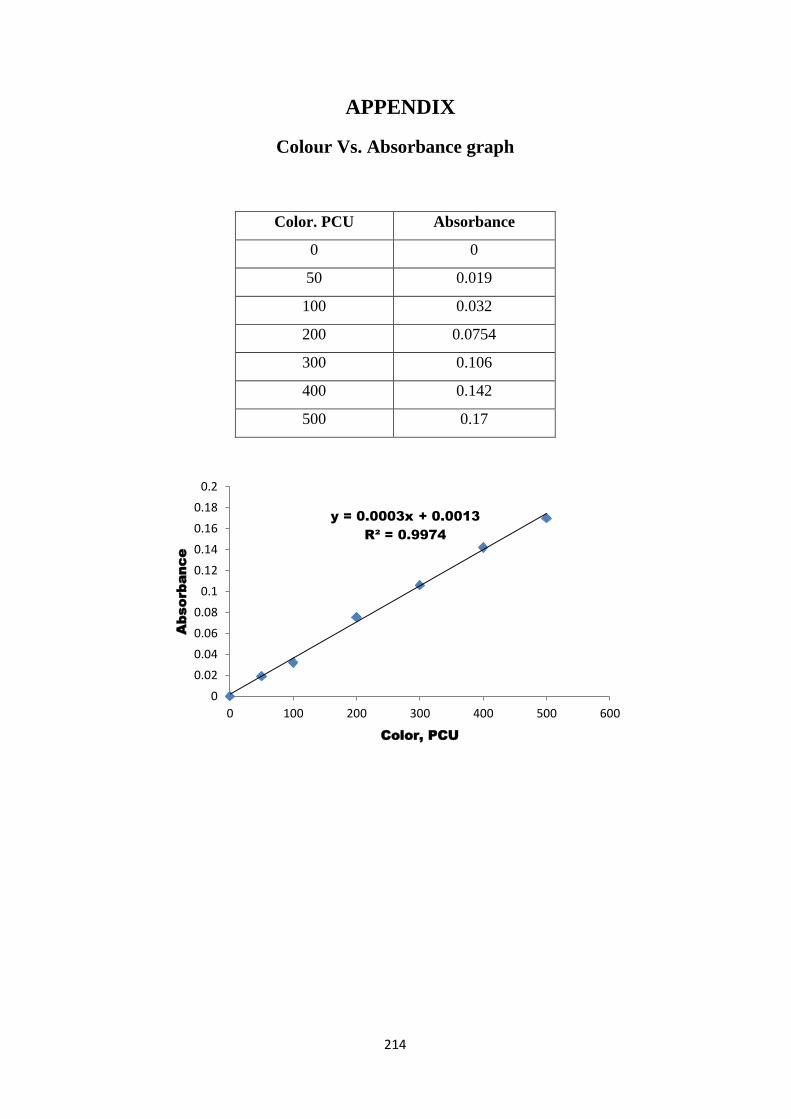
214
APPENDIX
Colour Vs. Absorbance graph
Color. PCU Absorbance
0 0
50 0.019
100 0.032
200 0.0754
300 0.106
400 0.142
500 0.17
y = 0.0003x + 0.0013
R² = 0.9974
0
0.02
0.04
0.06
0.08
0.1
0.12
0.14
0.16
0.18
0.2
0 100 200 300 400 500 600
Absorb
ance
Color, PCU
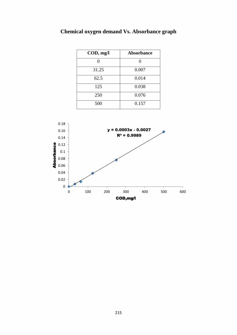
215
Chemical oxygen demand Vs. Absorbance graph
COD, mg/l Absorbance
0 0
31.25 0.007
62.5 0.014
125 0.038
250 0.076
500 0.157
y = 0.0003x - 0.0027
R² = 0.9989
0
0.02
0.04
0.06
0.08
0.1
0.12
0.14
0.16
0.18
0 100 200 300 400 500 600
Absorb
ance
COD,mg/l
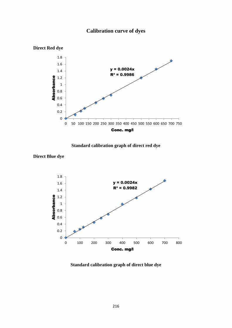
216
Calibration curve of dyes
Direct Red dye
Standard calibration graph of direct red dye
Direct Blue dye
Standard calibration graph of direct blue dye
y = 0.0024x
R² = 0.9986
0
0.2
0.4
0.6
0.8
1
1.2
1.4
1.6
1.8
0 50 100 150 200 250 300 350 400 450 500 550 600 650 700 750
Absorb
ance
Conc. mg/l
y = 0.0024x
R² = 0.9982
0
0.2
0.4
0.6
0.8
1
1.2
1.4
1.6
1.8
0 100 200 300 400 500 600 700 800
Absorb
ance
Conc. mg/l
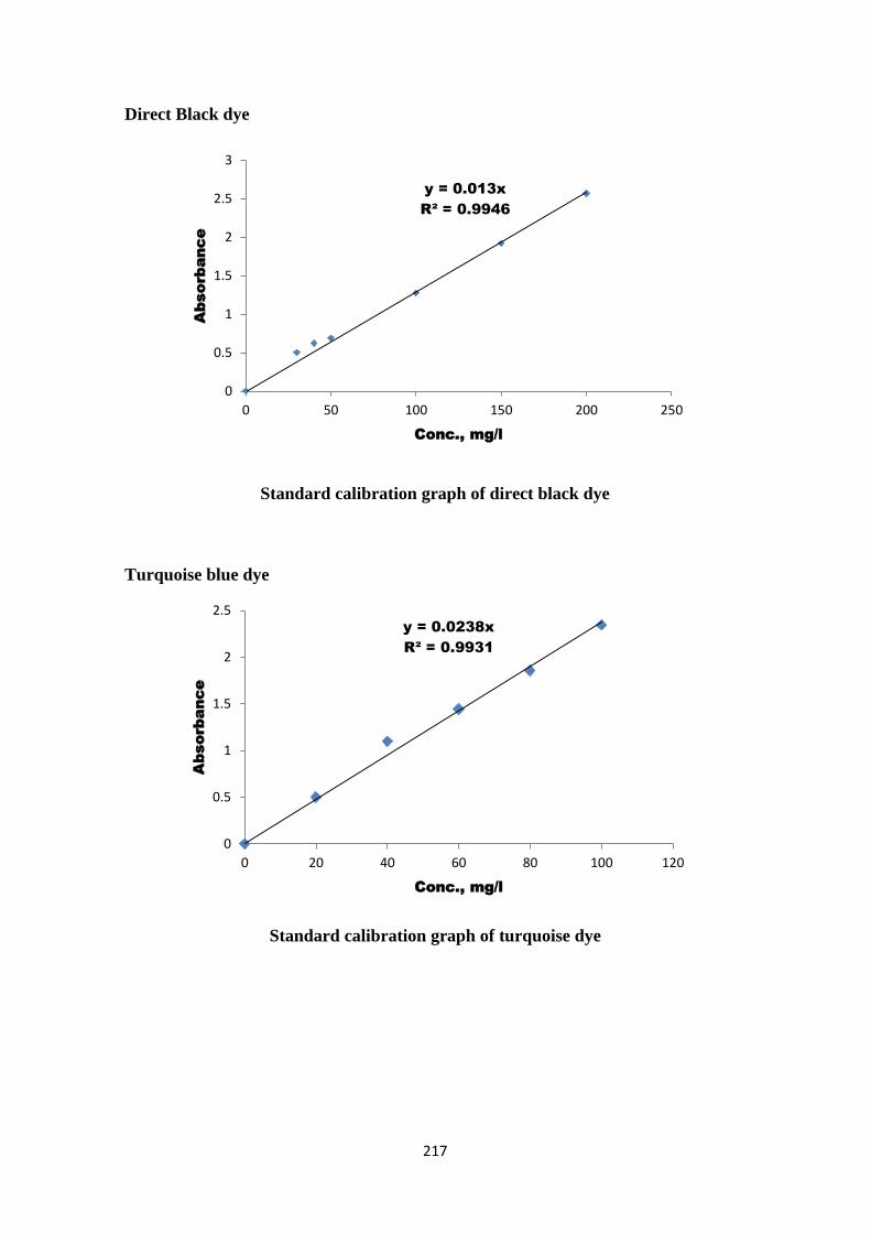
217
Direct Black dye
Standard calibration graph of direct black dye
Turquoise blue dye
Standard calibration graph of turquoise dye
y = 0.013x
R² = 0.9946
0
0.5
1
1.5
2
2.5
3
0 50 100 150 200 250
Absorb
ance
Conc., mg/l
y = 0.0238x
R² = 0.9931
0
0.5
1
1.5
2
2.5
0 20 40 60 80 100 120
Absorb
ance
Conc., mg/l
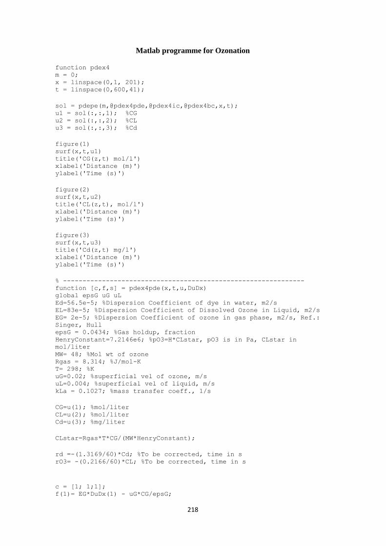
218
Matlab programme for Ozonation
function pdex4 m = 0; x = linspace(0,1, 201); t = linspace(0,600,41);
sol = pdepe(m,@pdex4pde,@pdex4ic,@pdex4bc,x,t); u1 = sol(:,:,1); %CG u2 = sol(:,:,2); %CL u3 = sol(:,:,3); %Cd
figure(1) surf(x,t,u1) title('CG(z,t) mol/l') xlabel('Distance (m)') ylabel('Time (s)')
figure(2) surf(x,t,u2) title('CL(z,t), mol/l') xlabel('Distance (m)') ylabel('Time (s)')
figure(3) surf(x,t,u3) title('Cd(z,t) mg/l') xlabel('Distance (m)') ylabel('Time (s)')
% -------------------------------------------------------------- function [c,f,s] = pdex4pde(x,t,u,DuDx) global epsG uG uL Ed=56.5e-5; %Dispersion Coefficient of dye in water, m2/s EL=83e-5; %Dispersion Coefficient of Dissolved Ozone in Liquid, m2/s EG= 2e-5; %Dispersion Coefficient of ozone in gas phase, m2/s, Ref.:
Singer, Hull epsG = 0.0434; %Gas holdup, fraction HenryConstant=7.2146e6; %pO3=H*CLstar, pO3 is in Pa, CLstar in
mol/liter MW= 48; %Mol wt of ozone Rgas = 8.314; %J/mol-K T= 298; %K uG=0.02; %superficial vel of ozone, m/s uL=0.004; %superficial vel of liquid, m/s kLa = 0.1027; %mass transfer coeff., 1/s
CG=u(1); %mol/liter CL=u(2); %mol/liter Cd=u(3); %mg/liter
CLstar=Rgas*T*CG/(MW*HenryConstant);
rd =-(1.3169/60)*Cd; %To be corrected, time in s rO3= -(0.2166/60)*CL; %To be corrected, time in s
c = [1; 1;1]; f(1)= EG*DuDx(1) - uG*CG/epsG;
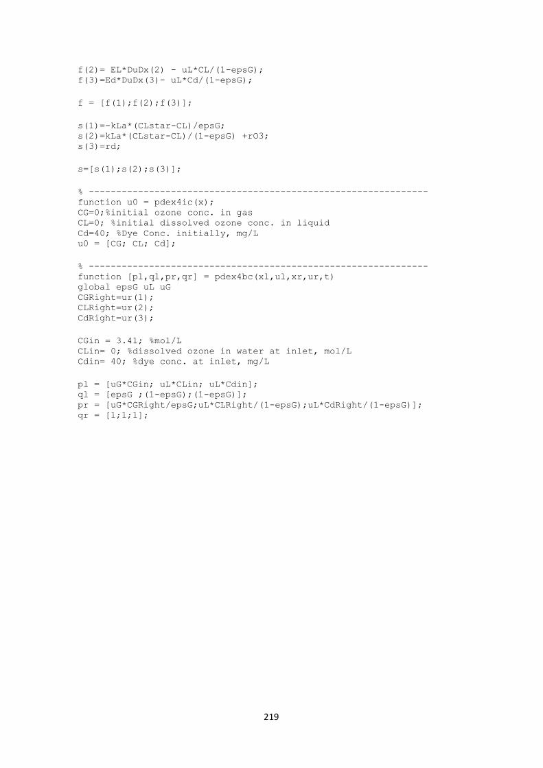
219
f(2)= EL*DuDx(2) - uL*CL/(1-epsG); f(3)=Ed*DuDx(3)- uL*Cd/(1-epsG);
f = [f(1);f(2);f(3)];
s(1)=-kLa*(CLstar-CL)/epsG; s(2)=kLa*(CLstar-CL)/(1-epsG) +rO3; s(3)=rd;
s=[s(1);s(2);s(3)];
% -------------------------------------------------------------- function u0 = pdex4ic(x); CG=0;%initial ozone conc. in gas CL=0; %initial dissolved ozone conc. in liquid Cd=40; %Dye Conc. initially, mg/L u0 = [CG; CL; Cd];
% -------------------------------------------------------------- function [pl,ql,pr,qr] = pdex4bc(xl,ul,xr,ur,t) global epsG uL uG CGRight=ur(1); CLRight=ur(2); CdRight=ur(3);
CGin = 3.41; %mol/L CLin= 0; %dissolved ozone in water at inlet, mol/L Cdin= 40; %dye conc. at inlet, mg/L
pl = [uG*CGin; uL*CLin; uL*Cdin]; ql = [epsG ;(1-epsG);(1-epsG)]; pr = [uG*CGRight/epsG;uL*CLRight/(1-epsG);uL*CdRight/(1-epsG)]; qr = [1;1;1];
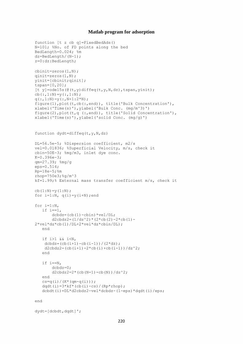
220
Matlab program for adsorption
function [t z cb q]=FixedBedAds() N=101; %No. of FD points along the bed BedLength=0.024; %m dz=BedLength/(N-1); z=0:dz:BedLength;
cbinit=zeros(1,N); qinit=zeros(1,N); yinit=[cbinit;qinit]; tspan=[0,20]; [t y]=ode15s(@(t,y)diffeq(t,y,N,dz),tspan,yinit); cb(:,1:N)=y(:,1:N); q(:,1:N)=y(:,N+1:2*N); figure(1),plot(t,cb(:,end)), title('Bulk Concentration'),
xlabel('Time(s)'),ylabel('Bulk Conc. (mg/m^3)') figure(2),plot(t,q (:,end)), title('Solid Concentration'),
xlabel('Time(s)'),ylabel('solid Conc. (mg/g)')
function dydt=diffeq(t,y,N,dz)
DL=56.5e-5; %Dispersion coefficient, m2/s vel=0.01836; %Superficial Velocity, m/s, check it cbin=50E-3; %mg/m3, inlet dye conc. K=0.396e-3; qm=27.39; %mg/g eps=0.514; Rp=18e-5;%m rhop=750e3;%g/m^3 kf=1.99;% External mass transfer coefficient m/s, check it
cb(1:N)=y(1:N); for i=1:N, q(i)=y(i+N);end
for i=1:N, if i==1, dcbdz=(cb(1)-cbin)*vel/DL; d2cbdz2=(1/dz^2)*(2*cb(2)-2*cb(1)-
2*vel*dz*cb(1)/DL+2*vel*dz*cbin/DL); end
if i>1 && i<N, dcbdz=(cb(i+1)-cb(i-1))/(2*dz); d2cbdz2=(cb(i+1)-2*cb(i)+cb(i-1))/dz^2; end
if i==N, dcbdz=0; d2cbdz2=2*(cb(N-1)-cb(N))/dz^2; end cs=q(i)/(K*(qm-q(i))); dqdt(i)=3*kf*(cb(i)-cs)/(Rp*rhop); dcbdt(i)=DL*d2cbdz2-vel*dcbdz-(1-eps)*dqdt(i)/eps;
end
dydt=[dcbdt,dqdt]';