Embed Size (px)
Citation preview

1
Treatment Performance of Direct Contact Membrane Distillation for Volatile, Semi-
Volatile and Non-Volatile Organic Contaminants in Water
Danbi Won
A thesis
submitted for the partial fulfillment of the
requirements for the degree of
Master of Science
in Civil Engineering
University of Washington
2017
Committee:
Edward P. Kolodziej
Gregory V. Korshin
Program Authorized to Offer Degree:
Civil & Environmental Engineering

2
Abstract
Treatment Performance of Direct Contact Membrane Distillation for Broad Spectrum of Organic
Contaminants in Water
Danbi Won
Chair of Supervisory Committee: Edward P. Kolodziej
Department of Civil and Environmental Engineering
A laboratory-scale direct contact membrane distillation (DCMD) system was analyzed for
treatment performances of a selection of volatile (V), semi-volatile (SV) and non-volatile (NV)
organic contaminants, pharmaceuticals and personal care products (PPCPs) and nitrosamines that
are of interest to water or wastewater treatment. A group of 32 organics, 8 nitrosamines, and 22
PPCPs were observed with acceptable mass recoveries (> 60%) in the system, with observed
recoveries well explained by their lower hydrophobicity (log Kow < 3) and less propensity to sorb
to DCMD system components. Due to their low volatility, and consistent with expectations derived
from Henry’s law partitioning coefficients (KH; where pKH = -logKH), NV solutes with pKH > 8
were rejected efficiently, with observed rejections of over 90%. Henry’s Law constants estimated
at 25°C were not fully predictive of treatment performance during DCMD, indicating that other
physical and chemical characteristics contribute to rejection. For example, moderate rejections
(i.e. 35% to 69%) were observed for some NV solutes with pKH < 8, as the 50°C feed temperatures
increased their apparent volatility in the system. Rejections for SV and V solutes were typically

3
lower, often more variable and sensitive to solute characteristics such as ionizability. In some cases,
dissociation constants ( pKa ) explained higher than expected rejection (e.g. 2-methyl-4,6-
dinitrophenol; pKa = 4.31) for ionizable solutes that were non-volatile at system pH. To account
for the time dependent characteristics of DCMD batch system, a least square curve fitting modeling
approach was used to evaluate the possibility for non-equilibrium, mass transfer limited conditions
for SV and V solutes. Permeate fluxes of each contaminant also were developed based on observed
DCMD data.
4
Acknowledgements
I am grateful to my adviser, Dr. Edward Kolodziej, for enabling and advising my research at the
University of Washington. I would like to express my gratitude to my second committee
member, Dr. Gregory Korshin, for his support through my master degree at the University of
Washington.
I would like to thank research fellows, Dr. Sage R. Hiibel and Kevin A. Salls for their advice and
contributions to my research.
I also wish to thank my family and fiancé for their incredible support and encouragement with
their kind words throughout the duration of my studies. I would especially like to thank Bosun
Gwon, Yongsuk Won, Hana Won, and Yoonbae Park.
Lastly, I wish to thank the United States Environmental Protection Agency Star Program for the
research grant support, which spiced up my persistent research efforts and enables my success.

5
Table of Contents
List of Figures................................................................................................................................. 7
List of Tables.................................................................................................................................. 8
Chapter 1: Introduction
Direct Contact Membrane Distillation Configuration........................................................ 9
Environmental Fate and Transport of contaminants......................................................... 10
Research Objectives.......................................................................................................... 11
Chapter 2: Material and Methods
2.1 DCMD System Setup.................................................................................................. 11
2.2 Experimental Protocol
2.2.1 Semi-volatile and volatile organics.............................................................. 12
2.2.2 Pharmaceuticals and Personal Care Products (PPCPs) ............................... 13
2.2.3 Nitrosamines................................................................................................ 15
Chapter 3: Results and Discussion
3.1 Mass Recovery............................................................................................................ 15
3.2 Rejection and Treatment Performance
3.2.1 Calculations.................................................................................................. 18
3.2.2. Comparison with modeled rejection........................................................... 19
3.2.3 Rejection as a function of solute volatility.................................................. 20
3.2.4 Rejection and dissociation constants........................................................... 22
3.2.5 Rejection comparison with literatures......................................................... 23
3.3 Temperature Dependence on Chemical Parameters
3.3.1 Henry’s constants......................................................................................... 24
6
3.3.2 Vapor pressures............................................................................................ 25
3.4 Contaminant Mass Flux and Transport
3.4.1 Mass flux of contaminants........................................................................... 26
3.4.2 Predict mass flux of contaminants............................................................... 27
3.4.3 Mass flux and resistances............................................................................. 29
Chapter 4: Conclusions................................................................................................................. 30
Works Cited ................................................................................................................................. 32

7
List of Figures
Figure 1: Schematic diagram of bench-scale DCMD system......................................................... 40
Figure 2: Observed mass recovery in the DCMD system.............................................................. 41
Figure 3: Correlation of observed mass recovery [%] during DCMD and octanol-water partition
coefficient, log Kow for semi-volatiles and volatiles.....................................................................42
Figure 4: Observed overall rejection of phenols (A) and anilines (B) over 48 hours in the DCMD
system............................................................................................................................................ 43
Figure 5: Theoretical rejection [%] models for the DCMD system, with rejection ranging from
100% to -400% in feed (A) and distillate (B), expressed as a function of time............................. 44
Figure 6: High rejection of 4-nitroaniline with concentration variation over time during
DCMD…………………………………………………………………………………………... 45
Figure 7: Intermediate rejection of benzyl alcohol with concentration variation over time during
DCMD........................................................................................................................................... 46
Figure 8: Modeled rejection of 3-methylphenol with concentration variation over time during
DCMD........................................................................................................................................... 47
Figure 9: Overall rejections of 32 semi-volatile and non-volatile organic compounds by DCMD
plotted against their Henry’s law constants values (shown as pKH) ............................................. 48
Figure 10: Overall rejections of 8 nitrosamines with increasing Henry’s law constants values
shown as pKH at 50°C.................................................................................................................... 49
Figure 11: Rejections with dissociation effect (pKa) for phenols and amines.............................. 50
Figure 12: Overall rejection of 23 non-volatile PPCPs by DCMD, Henry’s law constants values
shown as p𝐾𝐻 at 25°C.................................................................................................................... 51
Figure 13: Comparison of rejection values and Henry’s law constants (pKH) between this study,
Wijekoon, and Xie........................................................................................................................ 52
8
Figure 14: Correlation of ∆ rejection in feed and distillate [%] versus p(∆KH ) for an amine
group............................................................................................................................................. 53
Figure 15: Rejection differences for 8 nitrosamines between feed and distillate influenced by
vaporization enthalpy, vapor pressure difference at 25°C and 50°C, and permeate flux.............. 54
Figure 16: Percentage resistance in liquid phase of volatiles and semi-volatiles organic compounds
correlated with Henry’s law constants (KH) ................................................................................. 55
List of Tables
Table 1. Observed mass recoveries [%] of 65 non-volatiles, semi-volatiles, and volatiles based on
chemical group.............................................................................................................................. 35
Table 2. Observed rejection of 32 solutes divided into non-volatile (NV), semi-volatile (SV), and
volatile (V) based on their Henry’s law constants (pKH) and dissociation constants (pKa).......... 36
Table 3. Observed recovery and rejection data and physicochemical properties of 8 nitrosamines
and 23 PPCPs................................................................................................................................. 38
Table 4. Computational approaches to estimate diffusivities of organic solutes in gaseous phase
and liquid phase............................................................................................................................. 39

9
Chapter 1. Introduction
Membrane distillation (MD) is capable of targeted separation of organic chemicals, metals,
and salts to improve water quality of seawater or contaminated fresh waters. MD membranes are
hydrophobic, with micron-scale non-wetted pores that enable vapor phase transport through the
membrane after evaporation from the liquid phase. Unlike most membrane processes, MD
membranes operate at atmospheric pressure, reducing pumping costs and limiting pressure driven
accumulation of foulants at the membrane surface. Membrane distillation configurations include
direct contact MD (DCMD), air gap MD (AGMD), vacuum MD (VMD), and sweeping gas MD
(SWGMD).1-2
DCMD is the simplest configuration where the hydrophobic membrane is directly
contacted with the warm feed and cool distillate solutions. Temperature differences between the
feed and distillate surfaces in DCMD generate a partial vapor pressure difference across the
membrane, which is the driving force for mass transfer of water and volatile solutes. DCMD is
potentially a high efficiency separation process because increasing solute concentrations do not
substantially alter the partial vapor pressure of water.3 DCMD can be cost-effective because of its
simplicity to set up and operate, and it is potentially suitable for waste heat capture because only
a low temperature differential (20-50°C1) is required between feed and distillate. A solute, if
volatile, transports through the membrane by evaporation at the warm air-water interface on the
feed side followed by condensation at the cool air-water interface on the distillate side. Non-
volatile solutes such as ions and metals are efficiently concentrated in the feed because they cannot
transport across the membrane.2, 4 Thus, non-volatile contaminants such as inorganic salts, ionic
species, metals, and pathogenic micro-organisms typically exhibit near 100% rejection during MD,
implying potential applications for water or wastewater treatment. 5-6 7-8

10
When considering applications such as wastewater treatment and water reuse, the
capabilities of MD separation remain unclear because such complex feed streams typically contain
many semi-volatile and volatile solutes, and such solutes would be expected to transport through
the MD membrane. For solutes with some volatility, separation performance will be characterized
by partial rejection, and would be expected to scale with volatility. Indeed, concentration
enhancement in the distillate for those constituents that are more volatile than water is even
possible and would have substantial performance implications for highly volatile toxic or
hazardous pollutants.9 Wijekoon10 and Xie11 have shown that wastewater derived trace organic
compounds (TrOCs) such as pharmaceuticals, steroid hormones, phytoestrogens, and pesticides
with pKH >9 (Henry’s Law constants; pKH[𝑎𝑡𝑚 ∙ 𝑚3/ 𝑚𝑜𝑙] where pKH = − log KH ), all
classified as non-volatile, have removal efficiency >80% during MD, with most observed removals
near 100%. While promising, these results characterized performance for a relatively small subset
of the constituents of concern expected in impaired water resources.
Organic solutes can be classified as non-volatile (NV), semi-volatile (SV), and volatile (V)
to better understand and predict treatment performance during DCMD. With respect to volatility
and Henry’s law constants, typically evaluated at 25°C, NV contaminants are considered to have
pKH >6.52, SV with 5<pKH<6.52, and V with pKH <5.12 Estimating permeate flux [𝑘𝑔/𝑚2 ∙ ℎ] of
solutes during MD might also be useful as a tool to understand comparative transport and mass
transfer processes. For instance, low volatility constituents have very little permeate flux because
of their low vapor pressures, while higher permeate flux would be expected for more volatile
compounds due to their higher vapor pressures. Typically, interactions between organic
constituents and the membrane were assumed to not strongly affect transport because of the
thousand-fold size difference between angstrom-sized molecules and the micron-sized MD

11
membrane pore sizes, although complex chemical conditions at air water interfaces complicate
predictive capabilities. Permeate flux can be estimated by physiochemical properties such as mass
diffusivities, partial vapor pressures, and mass transfer coefficients, which may allow the
prediction of mass transport for water and wastewater contaminants in DCMD systems.
To assess separation performances for complex feed mixtures of water pollutants with
varying chemical characteristics, we evaluated the fate of water or wastewater derived non-volatile,
semi-volatile, and volatile organic contaminants in a bench scale DCMD system. Many regulated
contaminants of interest to water or wastewater treatment, potential applications for waste heat
driven DCMD, include those that are carcinogenic, highly mobile, toxic or aesthetically unpleasant,
and are somewhat volatile.13-15 Therefore, analytes evaluated in our system included PPCPs,
nitrosamines, and a suite of regulated organic contaminants.16 We included PPCPs such as caffeine
and carbamazepine because they are detected frequently in municipal wastewater effluents and
represent organic micropollutant classes typically used to evaluate the performance of advanced
wastewater treatment processes.17-19 With system data, we correlated observed rejections with
chemical parameters such as Henry’s law constants, enthalpy of vaporization, and dissociation
constants. The sensitivity of Henry’s law constants and vapor pressure to temperature was also
evaluated. While MD performance for non- or low volatility wastewater-derived contaminants has
been explored, MD performance for complex mixtures consisting of wastewater-derived
contaminants with diverse higher volatility characteristics has not been explored.20 Therefore, this
study was evaluated treatment performances for volatiles to non-volatile pollutants and
investigated physiochemical parameters influenced on their performances. This assessment is
intended to evaluate the potential use of DCMD for water quality improvement of volatile and
semi-volatile contaminants by DCMD.

12
Chapter 2. Material and methods
2.1 DCMD system setup
A bench scale DCMD system was used to evaluate treatment performances for the targeted
analytes. The system used a hydrophobic microporous polytetrafluoroethylene (PTFE) membrane
module (GE Osmonics, Minnetonka, MN), with a single PTFE active layer in the membrane
thickness of 67μm with a nominal pore size of 0.18μm and porosity of 80.1%.21 The DCMD system
(Figure 1) consists of a membrane cell, two low-pressure stainless steel gear drive pumps (Cole-
Palmer, USA), four thermocouples, two Kynar® gas sampling bags (Analytical Specialties Inc,
IL), a hot water bath (Thermo-Fisher Scientific, USA), a balance (A&D Weighing, USA), a
recirculating chiller, and a heat exchanger (Thermo-Fisher Scientific, USA).22 The membrane
module measures 155mm x 92mm x 3mm with an effective surface contact area of 143cm2.
Notably, special care was taken to design a system gas-tight to minimize possible losses of volatile
analytes via volatilization. Stainless steel tubing was also used to minimize adsorption to system
components if possible. The feed stream was circulated at 1L/min inside the membrane cell and
maintained 50° C by the hot water bath. The distillate stream was also circulated at 1L/min and
kept 25° C using a recirculating chiller combined with a heat exchanger. Temperatures in feed and
distillate inlets were monitored by four thermocouples and recorded by a computer connected to
LabView (Version 14.0.1.4008, National Instruments, Austin Texas, USA). Two gas tight sample
bags were installed in membrane cells at feed and distillate inlets and connected to two stainless
steel sampling valves to collect samples from feed and distillate reservoirs. (et al Salls)

13
2.2 Experimental protocol
2.2.1 Semi-volatile and volatile organics
A pre-made commercial standard (the 8270 “Megamix” standard, Restek, Bellefonte, PA)
of 76 volatile and semi-volatile chemicals was used to spike the bench scale DCMD system. All
of the chemicals in this standard are regulated or toxic pollutants of water, and they all are
amenable to analysis by EPA method 8270D. As this standard was dissolved in dichloromethane
(DCM), which is immiscible in water, the standard was first sonicated (5 min), then 15 mL of
methanol was added as a co-solvent. This DCM-methanol mixture was then added to a 4 L of
ultrapure water in a pre-cleaned amber glass bottle and equilibrated, with mixing, for 24 hours at
4 °C, prior to addition to the DCMD feed reservoir.
Samples from the DCMD system were collected in 1-L amber glass containers, without
headspace, chilled to 4 °C, spiked with deuterated standards, and solid-phase extracted (SPE) using
EPA Method 525.3 with DVB Speedisks (JT Baker). The SPE disks were shipped overnight on
ice to the Center for Urban Waters (Tacoma, WA) for analysis. Briefly, semi-volatile organics
were eluted from the SPE disks using ~10 mL acetone and methylene chloride. The extracts were
analyzed with gas chromatography-mass spectrometry using EPA method 8270D by the City of
Tacoma Environmental Services Laboratory, which is a Washington State Department of Ecology
accredited laboratory facility. Method reporting levels ranged from 1-10 µg/L, depending on the
analyte and volume extracted. Quality assurance-quality control samples included method blanks
and laboratory blank spikes, and all data used in this study passed QA/QC criteria. The experiment
was conducted twice (08/24/15 - 08/26/15; 01/02/16 – 01/04/16).
2.2.2 Pharmaceuticals and Personal Care Products (PPCPs)

14
DCMD system performance was also evaluated for a suite of wastewater-derived PPCPs
using analytical methods adapted from Keil and Neibauer (2009) and Vanderford et al. (2003). A
mixture of 30 PPCPs, mostly polar and recalcitrant compounds, dissolved in water was spiked into
4 L of ultrapure water in a pre-cleaned amber glass bottle and equilibrated for 24 hours (4 °C) prior
to addition. Samples were collected and shipped on ice to the Center for Urban Waters (Tacoma,
WA) for analysis. Prior to extraction, isotopically-labeled surrogate compounds in methanol were
added (nominal concentrations 10-250 μg/L), then samples were sequentially vacuum-filtered
through 0.7 µm glass fiber filter, 0.45 and 0.2 µm PEM filter. The pH was then adjusted to 8 ± 0.1
with 0.12 M hydrochloric acid or 0.19 M sodium hydroxide. Briefly, samples were SPE extracted
under vacuum at ~10 mL/min with pre-conditioned Oasis HLB cartridges (500 mg, Waters Corp.).
Cartridges were dried under ultra-high purity nitrogen gas, then eluted with 5 mL 10:90
methanol:MTBE (v:v) followed by 5 mL methanol. The eluant was concentrated to 75 µL with
ultra-high purity nitrogen gas in a 35°C water bath and transferred to a HPLC vial, with 1.425 mL
of pH = 2.8 acetic acid and 10 µL of isotopically-labeled internal standard solution.
Extracts were analyzed by high performance liquid chromatography-tandem mass
spectrometry, with a triple quadrupole mass analyzer (HPLC-MS/MS; Agilent 1290 HPLC,
Agilent 6460 triple quadrupole MS) using multiple reaction monitoring (MRM) and
positive/negative polarity switching. The HPLC column was an Agilent Zorbax Eclipse, 2.1 x 150
mm, dp= 3.5 µm. The injection volume was 20-100 µL; column temperature was 50°C. The mobile
phase was (A) pH = 2.8 acetic acid, and (B) 100% methanol. The mobile phase flow rate was 0.4
mL/min. The mobile phase gradient was: 95% A (t = 0 to 2 min); 95% A to 60% A (t = 2 to 6 min);
60% A (t = 6 to 13 min); 60% A to 10% A (t = 13 to 18 min); 10% A (t = 18 to 22.5 min); 10% A
to 95% A (t = 22.5 to 22.6 min); and 95% A (t = 22.6 to 27.5 min). The concentration of each

15
analyte was determined by isotope-dilution mass spectrometry and corrected based on recovery of
isotopically-labeled recovery surrogates.23
2.2.3 Nitrosamines
Eight nitrosamines were selected as analytes: nitrosomorpholine, nitrosopyrrolidine,
nitrosopiperidine, nitrosodimethylamine, nitrosomethylethylamine, nitrosodiethylamine,
nitrosodipropylamine, and nitrosobutylamine. They were analyzed by EPA 8270 method, and
dosed to the system with Appendix IX nitrosamine mix (Supelco, Bellefonte, PA.). One 1mL spike
mixture ampule holding 2000 μg of each nitrosamine was sonicated for 5 minutes, then added to
an amber glass bottle containing 4L ultrapure water at 5°C. The solution was equilibrated for 24
hours at 4 °C after addition, with mixing, then added to 14L of ultrapure water in the Kynar® bag
on the feed inlet. The initial feed and distillate volume were 18L and 3L respectively, with total
system volume of 21L. Feed and distillate samples (500mL) were collected every 8 hours over 48
hours, then solid phase extracted (activated charcoal SPE, Restek 521 cartridges). Samples were
analyzed using gas chromatography-tandem mass spectrometry (Varian 4000 Ion Trap GC-
MS/MS; positive chemical ionization with methanol, DB624 column, 30 m, 0.25 mm, 1.4 µm) and
isotope dilution analytical methods.24
Chapter 3. Results and discussion
3.1 Mass recovery
Pollutant fate in the DCMD system was first evaluated by estimating mass recovery for the
compounds added to the system. Mass recoveries of solutes were determined by mass balances
which estimated with volumetric and concentration data for each consecutive time measurement:

16
MT = (Cf×Vf) + (Cd×Vd) + Mloss (1)
In Eq. (1), Cf and Cd are concentrations in the feed and distillate, respectively. Vf and Vd refer to
the volume in feed and distillate, respectively. MT and Mloss refer to the total mass balances and
mass loss which was estimated by difference. Mass recoveries of each compound during MD at
given time were calculated as:
Mass recovery [%]𝑡=𝑖 =(MT)𝑡=𝑖
(MT)𝑡=0×100 (2)
Mass recoveries of 65 V, SV, and NV solutes during MD were calculated (Table 1). Eleven
out of 76 compounds spiked to the system exhibited low recovery, had analytical issues or failed
to pass QA/QC criteria, thus they were not considered further in this analysis. The 65 remaining
compounds were classified into “good recovery” and “poor recovery” groups in Figure 2. The
recoveries exceeding 60% were best characterized by log Kow value < 3, suggesting more polar
compounds with less affinity for hydrophobic sorption to system components (Figure 3). The
compounds, divided into 9 chemical groups, were organized by their observed recoveries: good
recovery group >60% (phenols, halogenated phenols, and anilines), intermediate recovery within
the group (some compounds above and some below 60%; phthalate, halogenated organic,
alcohol/ether, and benzidines/aromatic amines), and poor recovery <60% (halogenated benzene
and PAHs). Mass recoveries of compounds within the same chemical groups were generally
consistent, except for phthalates and halogenated organics which were more variable. A couple of
compounds, phenols and anilines, exhibited occasional recovery up to 157% which likely resulted
from analytical uncertainty.
Good recoveries for nitrosamines and PPCPs, a polar and soluble class of contaminants
common to wastewater effluent,25 were typical (Table 3), with values are mostly above 60% except
sulfathiazole, which exhibited 26% recovery and was not included in subsequent analysis. We did

17
observe that 20 out of 23 PPCPs and 3 out of 8 nitrosamines exhibited recoveries of over 100%,
and up to 250% in one case, during the run. While we are somewhat uncertain of the explanation
for this observation, we believe that some concentration dependent analytical effects (matrix
enhancement of ionization, etc) were occurring for these particular analytes in the feed as it
concentrated over time, thus systematically overestimating their concentrations. Because these
compounds were mostly NV, often with very low concentrations detected in the distillate, we do
not believe that this analytical uncertainty much affected our data interpretation.
Solutes with low recoveries, italicized in Table 1 and Table 3, indicate mass loss of solutes
in the system, including sorption to the membrane tubing surfaces, the feed and distillate reservoirs,
volatilization into the limited head space in the system, or reaction. Among the possibilities
explaining low recovery, sorption is likely the most plausible mechanism (Figure 2 and 3) for the
more hydrophobic compounds such as halogenated benzenes and PAHs (log Kow >4) that were
much more likely to demonstrate low recovery (0-22% recovery). Lost mass is most likely sorbed
to the hydrophobic MD membrane tubing or gas tight reservoirs, especially on the feed
components.26-27 Solvent rinses (methanol) performed after the experiment was complete were
able to recover many of these hydrophobic analytes from tubing and the membrane. Hydrophilic
compounds with log Kow < 3 exhibited good mass recoveries (>60%) during MD process, but
additional factors do affect recovery: 4-chloro-3-methylphenol (high recovery of 108% with log
Kow = 3.1) and naphthalene (low recovery of 28% with log Kow = 3.3) have similar log Kow values
but very different observed recoveries. All compounds with observed recovery less than 60% were
not included in subsequent data analysis.
3.2 Rejection and treatment performance

18
3.2.1 Calculations
Rejection (𝑅𝑖) of a solute in a membrane process, indicating an inability to pass across a
membrane barrier, is typically defined as 28:
𝑅𝑖(𝑡) = (1 −𝐶𝑑
𝐶𝑓) (𝑡)×100 (3)
Cf and Cd are concentrations [mg/L] in the feed and distillate, respectively in Eq (3). Rejection
calculations were done for each time interval when samples were collected. Likely due to dynamic
equilibrium conditions in a batch system, Figure 4 shows examples from two chemical classes
whose observed rejection R varied with time: (e.g. phenols and anilines). For certain compounds,
(e.g. 4-nitrophenol and 4-nitroaniline), rejections are near consistent with time. For other
compounds, (e.g. 2-nitrophenol and 3-methylphenol), rejections were not constant with time, and
consistently decreased as the experiment progressed. This trend was most, although not always,
apparent for more volatile compounds whose rejections were well below 100%, probably due to
changes in the driving force for mass transfer (system concentration gradients) over time.29 As
solutes left the feed side, crossed the membrane and built up in the distillate, some “reverse”
transport from the distillate back to the feed side would be expected. As system equilibrium
requires many such forward-reverse transport cycles, kinetic and mass transfer limitations might
best explain observed trends with time for such solutes. Also, as feed volumes decreased, the
constant pumping rate (1 L/min) provided solutes in the feed more “membrane contact time” later
in the experiment, potentially increasing mass transfer efficiency. These effects likely contributed
to changing solute fluxes into the distillate over time. Thus, complex, non-equilibrium dynamic
conditions are expected for batch DCMD systems, with mass transfer conditions varying across
the different solute chemical characteristics, as well as through time. These dynamics also imply
some limitations when equation (3) is used for batch systems because it does not explicitly include

19
a time component, especially as compounds get more volatile and mass transport mechanisms
become more sensitive to experimental conditions. Inconsistent transport rates between feed and
distillate sides likely arose from mass transfer limitations of molecular diffusion processes through
liquid and air films at the interface.30-32 Equation (3) thus represents an estimate of “overall
rejection” in the system, one that compares concentration differences in the feed and distillate
solutions to estimate performance and is most suitable for steady state and continuous processes.
3.2.2 Comparison with modeled rejection
To address some of the limitations of equation (3) for a batch system where time dependent
behaviors were observed, we also estimated system rejections by comparing observed
concentration over time for the feed and distillate solutions to predicted concentrations derived
theoretically. Modeled rejection in the system can be estimated by least square curve fitting to an
optimum rejection model fit by minimizing residuals (e.g. the difference concentrations estimated
by rejection model fits). Solutions for a “modeled” rejection, ranging from positive to negative,
are represented in Figure 5. For non-volatile solutes, when relative concentrations in the feed
increase rapidly over time, rejection of a solute is likely close to 100%. For more volatile
compounds, those with rejection down to 0%, or even negative rejections, their concentrations
increase far more slowly in the feed with concurrent increases in the distillate. The rejection can
even be highly negative (e.g. up to -320 for 2,4,6-trichlorophenol), which is explained by higher
solute flux through the membrane relative to water, driving rapid decreases over time for feed
concentrations.33
3.2.3 Rejection as a function of solute volatility

20
Examples of high, intermediate, and low rejection, as estimated by least square modeling,
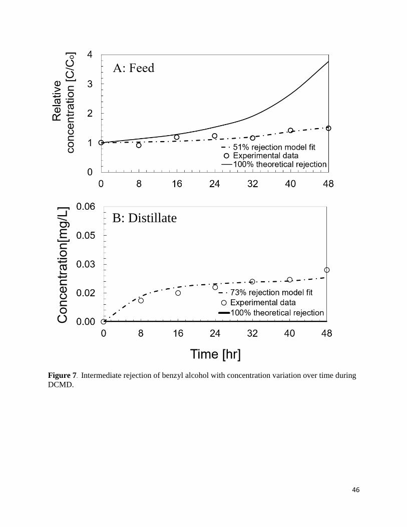
are presented (Figures 6-8). High rejection of 4-nitroaniline, a NV solute (pKH = 8.9), illustrates
near complete rejection (98% rejection via modeled rejection) with a clear and consistent
concentration increase in feed, and near non-detect concentration in distillate (Figure 6). As an
example of intermediate rejection, benzyl alcohol as a SV solute (pKH = 6.47) was observed at
different rejections in feed (51%) and permeate (73%) and near constant concentration in feed over
time (Figure 7). 3-methylphenol and 4-methylphenol, (pKH = 6.1 and 6.06, respectively) which
can easily travel through the DCMD membrane due to their volatility, are quickly detected in the
distillate, consistent with its concentration trends (Figure 8). This data modeling method can more
accurately account for trends in feed and distillate with time in a batch system by aligning
experimental data to those rejection model fits which are most consistent with theoretical
expectations (Figure 5). While the advantage of this approach is that it is possible to independently
estimate feed and distillate rejection as a function of time, there do exist cases where model fits
for feed and distillate rejections substantially diverge, implying some uncertainly and error with
the method. In some cases, these differences arise from analytical uncertainty or near non-detect
concentration data, yet explanations for other cases are less certain. In particular, we were not sure
whether such uncertainty is random or are biased by kinetic or hydraulic limitations to mass
transfer apparent within the system. Divergence in estimates for feed and distillate rejection, most
evident for more volatile solutes and those most sensitive to temperature,34 may be an artifact
derived from non-equilibrium conditions in the system.
Feed and distillate rejection via model fitting as well as overall rejection by equation (3),
using data at the final time, 48 hrs, were estimated and compared (Table 3). Overall rejection was
often close to an average of the observed feed and distillate model rejections; solutes with high

21
rejections typically are very consistent between the different approaches (Table 2). Eighteen
compounds fall within a 10% difference between overall rejection and model rejection. Also of
note, the model rejections from the modeled feed data are often more reliable and consistent in
comparison with estimates from distillate data, where less volatile compounds are detected at low
concentrations and with more uncertainty. For example, 19 compounds have feed rejections closest
to overall rejections, versus 9 compounds where distillate rejections are closest to overall rejections.
Rejection for nitrosamines with varying volatility ranged from negative to positive and
were well correlated to their Henry’s constant from 4.25 (volatile) to 7.0 (non-volatile; see Table
3). Polar functional groups were well correlated to high rejections and Henry’s constants at 50°C.
Chemical structures for each compound (Figure 10) indicate that highly soluble NPYR and NMOR
are non-volatile while less soluble NDBA is more volatile.38 Rejections for polar PPCPs that are
non-volatile also were well correlated to pKH (Figure 12) with mostly high rejections observed,
excluding a couple of solutes like propazine and cotenine. Due to what we think is matrix
dependent analytical bias for the PPCP run, feed rejections (along with recoveries) frequently
exceeded 100%. For example, carbamazepine was detected at 10.7 mg/L (140% rejection) in feed,
without detection in the distillate. Because very little mass was detected in distillate for these
compounds during MD, we are confident in our assessment of their DCMD performance, despite
some of the analytical uncertainties. The high rejections for pharmaceuticals indicate that we can
expect relatively effective treatment for these compounds during DCMD.
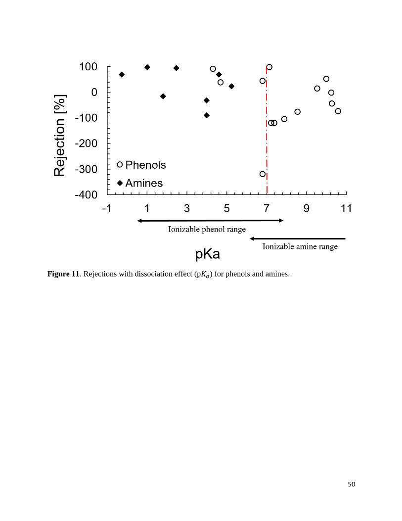
3.2.4 Rejection and dissociation constants
Observed rejection values are most consistent and near 100% for NV compounds with pKH
≥9 (see Figure 9). As volatility increases, solute rejections are less often consistent with

22
expectations from pKH, with lower rejection and more variability observed.11 For example, 2-
methyl-4,6-dinitrophenol (pKH= 5.85) has an observed rejection of 90% while a similarly volatile
compound 2-methylphenol (pKH= 5.92) exhibits substantially negative rejection around -45%.
This example indicates that pH also affects solute transport for ionizable compounds. In the case
of 2-methyl-4,6-dinitrophenol where the system pH was above the pKa for 4.31, most solute mass
was ionized and thus non-volatile, resulting in relatively high rejection (90%) for this semi-volatile
solute. For 2-methylphenol, largely un-ionized, mass transfer across the membrane was easier,
with -45% rejection (Figure 9). Removal efficiencies were notably influenced by solution pH and
dissociation constants were key parameters to explain differential rejection for ionizable
compounds with similar volatility.35-36 Percentage ionization for solutes is defined by37:
% ionization = [ionized / (ionized + neutral)] ×100% (4)
Phenols were ionized when pH was higher than their pKa values while amines were typically
neutral under the same conditions (Figure 11). Despite their substantial fraction of mass in the
ionized form, compounds such as 2,4,5- and 2,4,6-trichlorophenol (pKa 7.1 and 6.2, respectively)
had some of the lowest rejections observed in this study (rejections below -100 %). Because they
were apparently transported through membranes very effectively under the circumneutral pH
conditions of the system, despite the fact that they were not the most volatile solutes, acid base
dissociation kinetics did not seem to limit the kinetics of mass transfer through the DCMD
membrane. The neutral amines, including 2-, 3-, and 4-nitroaniline (pKa -0.28, 2.47, and 1.0)
concentrated in the feed because of their low volatility (pKH 7.23, 8.1, and 8.9), with some partial
transport (~70% rejection) observed for 2-nitroaniline. For neutral (un-ionized) solutes like aniline
and pyridine (pKH= 5.69 and 4.96, respectively), the influence of pH was less clear, although
rejections of these volatile compounds (~69%, 23%, respectively) were higher than might be

23
predicted by their low pKH values. System pH should be evaluated as a factor affecting solute
separation performance.
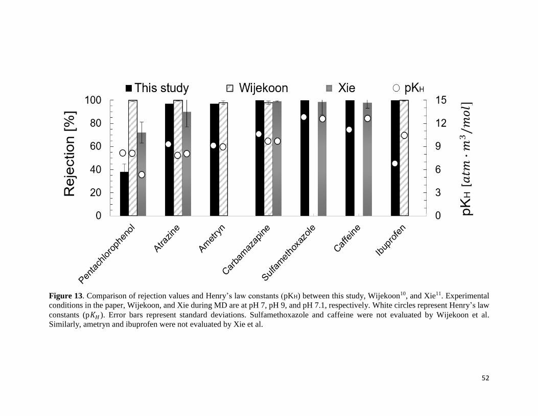
3.2.5 Rejection comparison with literature
Wijekoon et al.10 and Xie et al.11 also reported high removal efficiencies for trace organic
compounds, including PPCPs, and other non-volatile organics during DCMD. Seven wastewater
derived compounds were common to those studies and this study, allowing treatment performance
to be compared directly (Figure 13). Five compounds (i.e. ametryn, caffeine, carbamazepine,
ibuprofen, and sulfamethoxazole) exhibited near complete rejections both at pH 7.0 and 9.0,
consistent with their low volatility (pKH > 6.5) and hydrophobicity (log Kow < 3.0). For ionizable
compounds, their treatment performance might need additional studies to evaluate performance as
a function of system pH. For example, sulfamethoxazole is ionized at acidic pH values (i.e. pH
3.5, 4.5, and 5.5) and ibuprofen was negatively charged at pH of 8.0 as comparison to
carbamazepine’s neutrality across pH 3.5 to 7.5.36, 39 Pentachlorophenol and atrazine had lower
rejections, consistent with their volatility.
3.3 Temperature dependence for chemical parameters
3.3.1 Henry’s constants
For any particular solute, the sensitivity of volatility to temperature should impact expected
treatment performance during DCMD. Figure 9 also plots the temperature dependence of Henry’s
constants at our feed and distillate temperatures (𝑇𝑓 and 𝑇𝑑 ) of 25°C and 50°C, respectively.
Henry’s constants at 𝑇𝑓 (50°C) were corrected by Van’t Hoff equation and differences between
25°C and 50°C were shown by logarithmic values, p(∆KH ) = − log(𝐾𝐻,50°C−𝐾𝐻,25°C). Some
papers10, 40,41 noted pKH variations likely impact rejection after correction to 𝑇𝑓 (50–70 °C).

24
Likewise, solute volatilities have different sensitivity to temperature (derived from their enthalpy
of vaporization) that translates to different performance expectations for rejection. The difference
in volatility at feed and distillate temperatures can be expressed as a ∆KH gap (Figure 14). Larger
differences in ∆ KH , likely imply lower distillate to feed transport potential and increased
probability of non-equilibrium conditions for any specific solute. The enthalpy of vaporization
includes intermolecular forces by van der Waals forces, hydrogen bonding, and molecular surface
tension, all factors impacting solute transport.42 As typical for non-volatile compounds, PPCP
groups were less sensitive to temperature with p(∆KH) of 6 to 17 for the 𝑇𝑓 and 𝑇𝑑.36 For those NV
solutes which were most sensitive to temperature, based on their corrected pKH values at 50°C,
more transport than might be expected initially by observation of their Henry’s constants at 25°C
was evident. Moderate rejections (i.e. 35% to 69%) were observed by several NVs (i.e. dimethyl
phthalate, 2-nitroaniline, 2,4-dinitrotoluene, 2,4,6-tribromophenol, and pentachlorophenol)
despite their classifications as NV based on their 25°C pKH values. However, their corrected pKH
values at 𝑇𝑓, 50°C were lower or near 6.52, close to SV classification. The pKH values can increase
even more substantially at higher enthalpies of vaporization and larger temperature differences in
feed and distillate solutions. For example, if modifying the 𝑇𝑓 in MD to 70°C, the pKH value for
3-nitroaniline (overall R = 94%) would decrease to 6.84, which is similar with pentachlorophenol
(i.e. pKH 6.83) that was observed at 39% rejection at 𝑇𝑓, 50°C. Therefore, prediction of treatment
performances for contaminants based on their pKH value should start by first correcting their
pKH value to 𝑇𝑓 for the DCMD system of interest.
3.3.2 Vapor pressures

25
Vapor pressures for solutes also depended on temperature differences in feed and distillate.
Antoine equation and Grain Watson method were used to correct vapor pressures to 𝑇𝑓. Solutes
with bigger vapor pressure differences across the membranes, slowing distillate to feed transport,
likely resulted in non-equilibrium conditions for these solutes. This effects may have contributed
to observed rejection gaps (∆𝑅𝑖), or the difference between data modeled rejections based upon
feed and distillate concentrations (Figure 5). At high vapor pressures, solutes only require less
energy for vaporization.43-44 Therefore, V and SV solutes easily increased their mass transport
across membranes from feed to distillate.
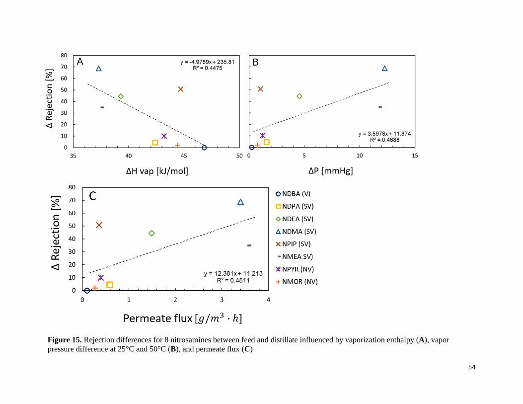
Inverse correlation of enthalpy of vaporization (∆Hvap) and vapor pressure differences (∆p )
were consistent with ∆𝑅𝑖 values except for two solutes: N-nitrosopiperidine (NPIP) and N-
nitrosomethylethylamine (NMEA, see Figure 15). NPIP and NMEA were greatly deviated from
the correlation of overall rejection to Henry’s constant at 50°C (Figure 10). Thus, for any specific
solute, the inter-relationships between Henry’s constants, vapor pressures, and enthalpy of
vaporization likely governs volatility, equilibrium, and mass transfer for solutes in DCMD systems.
3.4 Contaminant mass flux and transport
3.4.1 Mass flux of contaminants
Permeate flux is usually described in literature as a mean of evaluating the overall transport
of solutes from the feed to the distillate, especially while evaluating whether the flux is stable over
time as an aspect of membrane performance.10-11, 40 Typically, permeate fluxes of solutes such as
wastewater contaminants are not evaluated because most compounds separated by MD systems
are non-volatile and expected to concentrate in the feed. However, given the range of solute
26
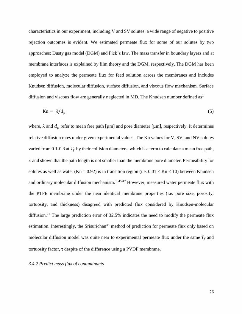
characteristics in our experiment, including V and SV solutes, a wide range of negative to positive
rejection outcomes is evident. We estimated permeate flux for some of our solutes by two
approaches: Dusty gas model (DGM) and Fick’s law. The mass transfer in boundary layers and at
membrane interfaces is explained by film theory and the DGM, respectively. The DGM has been
employed to analyze the permeate flux for feed solution across the membranes and includes
Knudsen diffusion, molecular diffusion, surface diffusion, and viscous flow mechanism. Surface
diffusion and viscous flow are generally neglected in MD. The Knudsen number defined as1
Kn = 𝜆/𝑑𝑝 (5)
where, 𝜆 and 𝑑𝑝 refer to mean free path [µm] and pore diameter [µm], respectively. It determines
relative diffusion rates under given experimental values. The Kn values for V, SV, and NV solutes
varied from 0.1-0.3 at 𝑇𝑓 by their collision diameters, which is a term to calculate a mean free path,
𝜆 and shown that the path length is not smaller than the membrane pore diameter. Permeability for
solutes as well as water (Kn = 0.92) is in transition region (i.e. 0.01 < Kn < 10) between Knudsen
and ordinary molecular diffusion mechanism.1, 45-47 However, measured water permeate flux with
the PTFE membrane under the near identical membrane properties (i.e. pore size, porosity,
tortuosity, and thickness) disagreed with predicted flux considered by Knudsen-molecular
diffusion.21 The large prediction error of 32.5% indicates the need to modify the permeate flux
estimation. Interestingly, the Srisurichan45 method of prediction for permeate flux only based on
molecular diffusion model was quite near to experimental permeate flux under the same 𝑇𝑓 and
tortuosity factor, τ despite of the difference using a PVDF membrane.
3.4.2 Predict mass flux of contaminants
27
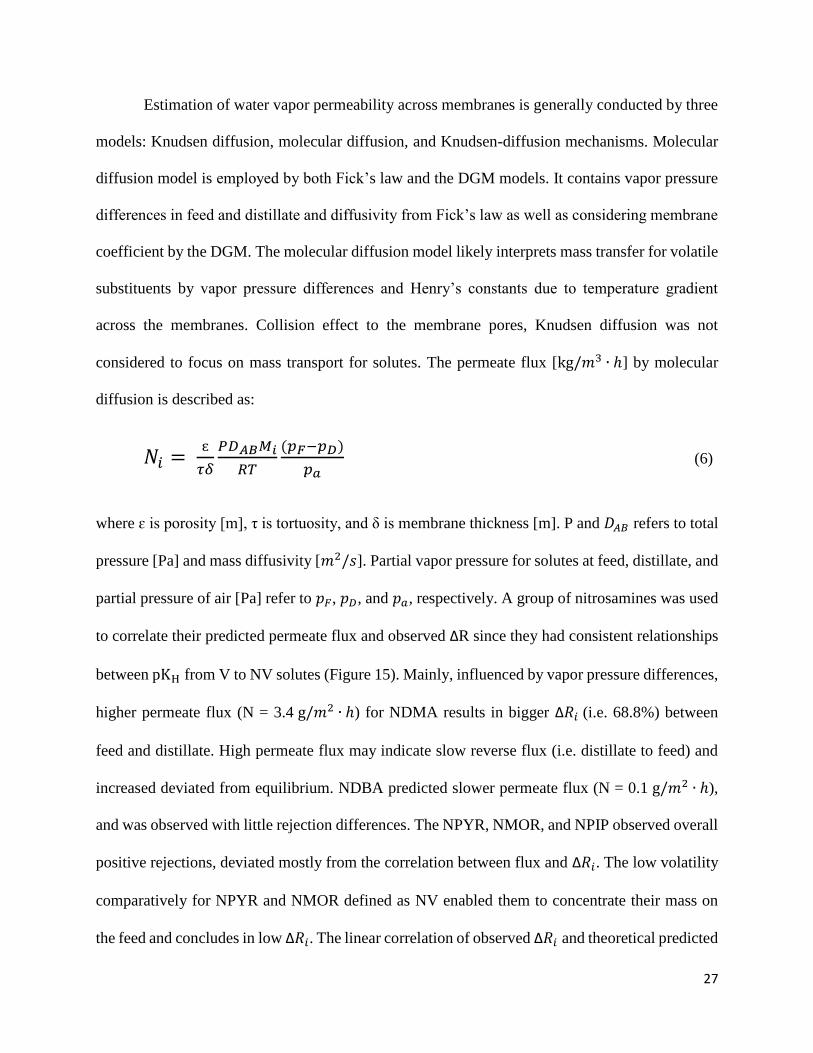
Estimation of water vapor permeability across membranes is generally conducted by three
models: Knudsen diffusion, molecular diffusion, and Knudsen-diffusion mechanisms. Molecular
diffusion model is employed by both Fick’s law and the DGM models. It contains vapor pressure
differences in feed and distillate and diffusivity from Fick’s law as well as considering membrane
coefficient by the DGM. The molecular diffusion model likely interprets mass transfer for volatile
substituents by vapor pressure differences and Henry’s constants due to temperature gradient
across the membranes. Collision effect to the membrane pores, Knudsen diffusion was not
considered to focus on mass transport for solutes. The permeate flux [kg/𝑚3 ∙ ℎ] by molecular
diffusion is described as:
𝑁𝑖 = ɛ
𝜏𝛿
𝑃𝐷𝐴𝐵𝑀𝑖
𝑅𝑇
(𝑝𝐹−𝑝𝐷)
𝑝𝑎 (6)
where ɛ is porosity [m], τ is tortuosity, and δ is membrane thickness [m]. P and 𝐷𝐴𝐵 refers to total
pressure [Pa] and mass diffusivity [𝑚2/𝑠]. Partial vapor pressure for solutes at feed, distillate, and
partial pressure of air [Pa] refer to 𝑝𝐹, 𝑝𝐷, and 𝑝𝑎, respectively. A group of nitrosamines was used
to correlate their predicted permeate flux and observed ∆R since they had consistent relationships
between pKH from V to NV solutes (Figure 15). Mainly, influenced by vapor pressure differences,
higher permeate flux (N = 3.4 g/𝑚2 ∙ ℎ) for NDMA results in bigger ∆𝑅𝑖 (i.e. 68.8%) between
feed and distillate. High permeate flux may indicate slow reverse flux (i.e. distillate to feed) and
increased deviated from equilibrium. NDBA predicted slower permeate flux (N = 0.1 g/𝑚2 ∙ ℎ),
and was observed with little rejection differences. The NPYR, NMOR, and NPIP observed overall
positive rejections, deviated mostly from the correlation between flux and ∆𝑅𝑖. The low volatility
comparatively for NPYR and NMOR defined as NV enabled them to concentrate their mass on
the feed and concludes in low ∆𝑅𝑖. The linear correlation of observed ∆𝑅𝑖 and theoretical predicted

28
permeate flux indicate a possibility to estimate an equilibrium state of solutes via their permeability
across the membranes.
3.4.3 Mass flux and resistances
Inverse correlation with the permeate flux is a resistance in the two phases, gas and liquid.
The two resistance model developed by Whitman31enables to estimate gas transfer rates and the
flux determined by molecular diffusion. Resistance in liquid phase (𝑅𝐿) was analyzed because it
is more affected by molecular movement in the solution than in gas phase. Volatile substituents
which are less soluble are consistently decreased their mass transfer rates, influenced by 𝑅𝐿. The
𝑅𝐿 is regarded as the ratio of the driving force to the rate of mass transfer and defined as28
𝑅𝐿 = 𝐻
𝐻 +𝑅𝑇(𝑘𝐿𝑘𝐺
) (7)
where 𝐻, R, and T mean Henry’s constants [𝑎𝑡𝑚 ∙ 𝑚3/ 𝑚𝑜𝑙], the gas constant [𝑎𝑡𝑚 ∙ 𝑚3/ 𝐾 ∙
𝑚𝑜𝑙] , and temperature [K]. Mass transfer coefficients for gas and liquid ( 𝑘𝐺 and 𝑘𝐿 ) were
estimated based on mass diffusivities in each phase. The eleven approaches for diffusivities
including a temperature dependence at 𝑇𝑓 were given (Table 4) and used to calculate the 𝑅𝐿.43
Calculated 𝑅𝐿 based on the seven equations were compared with Chapra’s resistance estimated in
two systems: great lakes and small sheltered lakes.30 The 𝑅𝐿 correlated by fourth equation of
diffusivity represented almost close to “small sheltered lakes system” (See Figure 16). Our
experimental DCMD system was covered in stainless steel and estimated not interrupted by any
other obstacles, which is similar with “the small sheltered lakes system” free from wind impacts.
This system was controlled by resistances in liquid phase for the mass transfer than another system
such as great lakes. The seven resistance graphs at 𝑇𝑑 , 25°C deviates within 1-5% standard

29
deviation from pKH, 2.41 to 4.8. The mostly diverged range (i.e. pKH 3.2 – 4.8) is in the middle of
gas and liquid controlled so expected controlled by both gas and liquid film. Temperature
dependence on resistance is also shown that higher Henry’s constants and mass transfer
coefficients at 𝑇𝑓 shift the resistance control to the liquid film. One note for the plot is that the
𝑅𝐿 is estimable for mostly volatiles with pKH < 5. The SV and NVs are likely predicted their
resistance in gas phase due to inclined to be more gas-phase controlled. The resistance can be
combined with permeate flux to determine their mass transfer in membranes: volatiles controlled
by liquid phase likely transport slower in the solution while semi-volatiles and non-volatiles
moderately move in gas phase due to controlled by gas phase.
Chapter 4. Conclusion
We conducted a DCMD experiment with a subset of volatile, semi-volatile and non-volatile
contaminants to determine their treatment performances in relation to their physiochemical
parameters. Solutes defined as non-volatile with pKH > 7 at feed temperature were observed at
nearly complete rejections in the DCMD system, but volatiles and semi-volatile solutes exhibited
separation efficiencies from negative to positive values. Acid dissociation constant, pKa was one
parameter that clearly influenced rejections for some solutes by reducing overall solutes volatility
(i.e. 2-methyl-4,6-dinitrophenol) when ionized at DCMD system conditions. Modeled rejections
independently based upon feed and distillate data demonstrate a wide range of rejection outcomes
for system components, from zero to – 580%, with solute transport driven by the temperature and
volatility differences across the membrane. The ∆R values were inter-correlated to chemical
properties and were sensitive to temperature dependence, Henry’s constant, enthalpy of

30
vaporizations, vapor pressure difference, and permeate fluxes. The different chemical
characteristics for solutes between feed and distillate membrane interfaces results in differential
equilibrium and permeability through the membranes, indicating that Henry’s constant KH, the
typical metric of volatility, is not always fully predictive of DCMD rejection. More detailed and
accurate estimates of mass transport across the membranes derived from first principles (such as
chemical potential) should be estimated from physical parameters such as mass diffusivities and
mass transfer coefficients to better understand fate outcomes for solutes with some volatility
attributes.
Nomenclature
C concentration (mg/L)
𝑑𝑝 pore diameter (µm)
𝐷𝐴𝐵 mass diffusivity from A to B phase(𝑚2/𝑠)
Ka acid dissociation constant (dimensionless)
𝑘𝐺 mass transfer coefficient in gas phase (m/s)
KH Henry’s constant (𝑎𝑡𝑚 ∙ 𝑚3/ 𝑚𝑜𝑙)
𝑘𝐿 mass transfer coefficient in liquid phase (m/s)
Kn Knudsen number (dimensionless)
Kow Octanol-Water partition coefficient (dimensionless)
M molecular weight (g/mol)
Mloss mass loss (g)
MT total mass balance (g)
Ni permeate flux of i (g/𝑚3 ∙ ℎ)
p partial vapor pressure (pa)

31
P total pressure (pa)
R universal gas constant (𝑎𝑡𝑚 ∙ 𝑚3/ 𝐾 ∙ 𝑚𝑜𝑙 )
𝑅𝑖 rejection of i (%)
𝑅𝐿 resistance in liquid phase
t time (min)
T temperature (K)
V volume (L)
Greek symbols
𝜆 mean free path (µm)
ɛ porosity (m]
τ tortuosity (dimensionless)
δ membrane thickness (m)
Subscripts
a air
f feed
d distillate

32
Works Cited
1. Khayet, M., Membrane distillation : principles and applications. Amersterdam ; Boston :
Elsevier: Amersterdam ; Boston, 2011.
2. Alkhudhiri, A.; Darwish, N.; Hilal, N., Membrane distillation: A comprehensive review.
Desalination 2012, 287, 2-18.
3. Martinetti, C. R.; Childress, A. E.; Cath, T. Y., High recovery of concentrated RO brines
using forward osmosis and membrane distillation. Journal of Membrane Science 2009, 331 (1-
2), 31-39.
4. Lawson, K. W.; Lloyd, D. R., Membrane distillation. Journal of Membrane Science
1997, 124 (1), 1-25.
5. Curcio, E.; Drioli, E., Membrane distillation and related operations - A review.
Separation and Purification Reviews 2005, 34 (1), 35-86.
6. Khayet, M., Membranes and theoretical modeling of membrane distillation: A review.
Advances in Colloid and Interface Science 2011, 164 (1-2), 56-88.
7. Alkhudhiri, A.; Darwish, N.; Hilal, N., Treatment of saline solutions using Air Gap
Membrane Distillation: Experimental study. Desalination 2013, 323, 2-7.
8. Cath, T. Y.; Adams, V. D.; Childress, A. E., Experimental study of desalination using
direct contact membrane distillation: a new approach to flux enhancement. Journal of Membrane
Science 2004, 228 (1), 5-16.
9. Tomaszewska, M., Membrane distillation - Examples of applications in technology and
environmental protection. Polish Journal of Environmental Studies 2000, 9 (1), 27-36.
10. Wijekoon, K. C.; Hai, F. I.; Kang, J. G.; Price, W. E.; Cath, T. Y.; Nghiem, L. D.,
Rejection and fate of trace organic compounds (TrOCs) during membrane distillation. Journal of
Membrane Science 2014, 453, 636-642.
11. Xie, M.; Nghiem, L. D.; Price, W. E.; Elimelech, M., A Forward Osmosis-Membrane
Distillation Hybrid Process for Direct Sewer Mining: System Performance and Limitations.
Environmental Science & Technology 2013, 47 (23), 13486-13493.
12. Zhang, C., Fundamentals of environmental sampling and analysis. Hoboken, N.J. :
Wiley-Interscience: Hoboken, N.J., 2007.
13. Snyder, S. A., Occurrence, treatment, and toxicological relevance of EDCs and
pharmaceuticals in water. Ozone-Science & Engineering 2008, 30 (1), 65-69.
14. Snyder, S. A.; Benotti, M. J., Endocrine disruptors and pharmaceuticals: implications for
water sustainability. Water Science and Technology 2010, 61 (1), 145-154.
15. Chary, N. S.; Fernandez-Alba, A. R., Determination of volatile organic compounds in
drinking and environmental waters. Trends in Analytical Chemistry 2011.
16. Plumlee, M. H.; Lopez-Mesas, M.; Heidlberger, A.; Ishida, K. P.; Reinhard, M., N-
nitrosodimethylamine (NDMA) removal by reverse osmosis and UV treatment and analysis via
LC-MS/MS. Water Research 2008, 42 (1-2), 347-355.
17. Daneshvar, A.; Aboulfadl, K.; Viglino, L.; Broseus, R.; Sauve, S.; Madoux-Humery, A.
S.; Weyhenmeyer, G. A.; Prevost, M., Evaluating pharmaceuticals and caffeine as indicators of
fecal contamination in drinking water sources of the Greater Montreal region. Chemosphere
2012, 88 (1), 131-139.
18. Miao, X. S.; Yang, J. J.; Metcalfe, C. D., Carbamazepine and its metabolites in
wastewater and in biosolids in a municipal wastewater treatment plant. Environmental Science &
Technology 2005, 39 (19), 7469-7475.
33
19. Carballa, M.; Omil, F.; Lema, J. M.; Llompart, M.; Garcia-Jares, C.; Rodriguez, I.;
Gomez, M.; Ternes, T., Behavior of pharmaceuticals, cosmetics and hormones in a sewage
treatment plant. Water Research 2004, 38 (12), 2918-2926.
20. Gryta, M.; Tomaszewska, M.; Karakulski, K., Wastewater treatment by membrane
distillation. Desalination 2006, 198 (1), 67-73.
21. Rao, G.; Hiibel, S. R.; Childress, A. E., Simplified flux prediction in direct- contact
membrane distillation using a membrane structural parameter. Desalination 2014, 351, 151-162.
22. Gustafson, R. D.; Murphy, J. R.; Achilli, A., A stepwise model of direct contact
membrane distillation for application to large- scale systems: Experimental results and model
predictions. Desalination 2016, 378, 14-27.
23. James, C. A.; Miller-Schulze, J. P.; Ultican, S.; Gipe, A. D.; Baker, J. E., Evaluating
Contaminants of Emerging Concern as tracers of wastewater from septic systems. Water
Research 2016, 101, 241-251.
24. Holady, J. C.; Trenholm, R. A.; Snyder, S. A., Use of Automated Solid-Phase Extraction
and GC-MS/MS to Evaluate Nitrosamines in Water Matrices. American Laboratory 2012, 44
(3), 25-30.
25. Snyder, S. A.; Westerhoff, P.; Yoon, Y.; Sedlak, D. L., Pharmaceuticals, Personal Care
Products, and Endocrine Disruptors in Water: Implications for the Water Industry.
Environmental Engineering Science 2003, 20 (5), 449-469.
26. Quantitative drug design; a critical introduction, 2d ed. Ringgold Inc: Portland, 2010;
Vol. 34.
27. Yoon, Y.; Westerhoff, P.; Snyder, S. A.; Wert, E. C.; Yoon, J., Removal of endocrine
disrupting compounds and pharmaceuticals by nanofiltration and ultrafiltration membranes.
Desalination 2007, 202 (1), 16-23.
28. Benjamin, M. M., Water Quality Engineering Physical / Chemical Treatment Processes.
Hoboken : Wiley: Hoboken, 2013.
29. Hoek, E. M. V.; Elimelech, M., Cake- enhanced concentration polarization: a new
fouling mechanism for salt- rejecting membranes. Environmental science & technology
2003, 37 (24), 5581.
30. Chapra, S. C., Surface water-quality modeling. Long Grove, Ill. : Waveland Press: Long
Grove, Ill., 2008.
31. Whitman, W. G., The two film theory of gas absorption. International Journal of Heat
and Mass Transfer 1962, 5 (5), 429-433.
32. Nghiem, L. D.; Schäfer, A. I.; Elimelech, M., Removal of natural hormones by
nanofiltration membranes: measurement, modeling, and mechanisms. Environmental science
& technology 2004, 38 (6), 1888.
33. Cho, C. H.; Oh, K. Y.; Kim, S. K.; Yeo, J. G.; Sharma, P., Pervaporative seawater
desalination using NaA zeolite membrane: Mechanisms of high water flux and high salt
rejection. Journal of Membrane Science 2011, 371 (1-2), 226-238.
34. Banat, F. A.; Simandl, J., Theoretical and experimental study in membrane distillation.
Desalination 1994, 95 (1), 39-52.
35. Ozaki, H.; Li, H., Rejection of organic compounds by ultra- low pressure reverse osmosis
membrane. Water Research 2002, 36 (1), 123-130.
36. Nghiem, L. D.; Schäfer, A. I.; Elimelech, M., Pharmaceutical retention mechanisms by
nanofiltration membranes. Environmental science & technology 2005, 39 (19), 7698.

34
37. Remington, J. P.; Beringer, P., Remington : the science and practice of pharmacy. 21st
ed. ed.; Philadelphia : Lippincott Williams & Wilkins: Philadelphia, 2006.
38. Mitch, W.; Sharp, J.; Trussell, R.; Valentine, R.; Alvarez-Cohen, L.; Sedlak, D. L., N-
nitrosodimethylamine ( NDMA) as a drinking water contaminant: A review. In Environ. Eng.
Sci., 2003; Vol. 20, pp 389-404.
39. Xie, M.; Price, W. E.; Nghiem, L. D., Rejection of pharmaceutically active compounds
by forward osmosis: Role of solution pH and membrane orientation. Separation and Purification
Technology 2012, 93, 107-114.
40. Naidu, G.; Jeong, S.; Choi, Y.; Vigneswaran, S., Membrane distillation for wastewater
reverse osmosis concentrate treatment with water reuse potential. Journal of Membrane Science
2017, 524, 565-575.
41. Al-Obaidani, S.; Curcio, E.; Macedonio, F.; Di Profio, G.; Al-Hinai, H.; Drioli, E.,
Potential of membrane distillation in seawater desalination: Thermal efficiency, sensitivity study
and cost estimation. Journal of Membrane Science 2008, 323 (1), 85-98.
42. Schwarzenbach, R. P., Environmental organic chemistry. 2nd ed. ed.; Hoboken, N.J. :
Wiley: Hoboken, N.J., 2003.
43. Zaitsau, D. H.; Kabo, G. J.; Strechan, A. A.; Paulechka, Y. U.; Tschersich, A.; Verevkin,
S. P.; Heintz, A., Experimental vapor pressures of 1- alkyl- 3- methylimidazolium
bis( trifluoromethylsulfonyl) imides and a correlation scheme for estimation of vaporization
enthalpies of ionic liquids. The journal of physical chemistry. A 2006, 110 (22), 7303.
44. Chickos, J. S.; Hanshaw, W., Vapor Pressures and Vaporization Enthalpies of the n -
Alkanes from C 21 to C 30 at T = 298.15 K by Correlation Gas Chromatography. J. Chem. Eng.
Data 2004, 49 (1), 77-85.
45. Srisurichan, S.; Jiraratananon, R.; Fane, A. G., Mass transfer mechanisms and transport
resistances in direct contact membrane distillation process. Journal of Membrane Science 2006,
277 (1), 186-194.
46. Alicia Kyoungjin, A.; Eui-Jong, L.; Jiaxin, G.; Sanghyun, J.; Jung-Gil, L.; Noreddine, G.,
Enhanced vapor transport in membrane distillation via functionalized carbon nanotubes anchored
into electrospun nanofibres. Scientific Reports 2017, 7.
47. Brodkey, R. S., Transport phenomena : a unified approach. New York : McGraw-Hill:
New York, 1988.
48. Fuller, E. N.; Schettler, P. D.; Giddings, J. C., NEW METHOD FOR PREDICTION OF
BINARY GAS- PHASE DIFFUSION COEFFICIENTS. Ind. Eng. Chem. 1966, 58 (5), 18-27.
49. A new method for prediction of binary gas- phase diffusion coefficients.: E N Fuller et
al. , Ind Eng Chem , 58 , 1966, 18–27. 1966; Vol. 16, pp 551-551.
50. Bird, R. B., Transport phenomena. 2nd, Wiley international ed. ed.; New York : J. Wiley:
New York, 2002.
51. Hayduk, W.; Laudie, H., Prediction of diffusion coefficients for nonelectrolytes in dilute
aqueous solutions. AIChE Journal 1974, 20 (3), 611-615.
52. Einstein, A., Investigations on the theory of the Brownian movement. New York : Dutton:
New York, 1915.

35
Table 1. Observed mass recoveries [%] of 65 non-volatiles, semi-volatiles, and volatiles based on
chemical group. Three categories of good (> 60%), intermediate (combined with good and poor
recovery), and poor (< 60%) recovery are used to classify each group. 33 solutes with < 60%
recoveries are italicized. SD [%] refers to standard deviation.
“Good recovery” Recovery
[%]
SD
[%] “Intermediate recovery”
Recovery
[%]
SD
[%] “Poor recovery”
Recovery
[%]
SD
[%]
Phenols Phthalate Halogenated benzene
2,4-Dimethylphenol 117 12 Butyl benzyl phthalate 14 5 1,2,4-Trichlorobenzene 14 30 2-Methyl-4,6-
dinitrophenol 145 23 Diethylphthalate 88 17 1,2-Dichlorobenzene 31 25
2-Methylphenol 113 9 Dimethyl
phthalate 103 21 1,3-Dichlorobenzene 27 26
2-Nitrophenol 115 11 Di-n-butylphthalate 19 6 1,4-Dichlorobenzene 27 26
3-Methylphenol 114 10 Di-n-Octyl phthalate 5 4 Hexachlorobenzene 4 0
4-Nitrophenol 157 27
Phenol 85 9 Halogenated organic PAHs
Hexachloroethane 22 6 Naphthalene 28 5
Halogenated phenols Hexachlorobutadiene 4 0 Acenaphthene 15 30
2,4,5-Trichlorophenol 80 12 Hexachlorocyclopentadiene 3 0 Acenaphthylene 19 29
2,4,6-Tribromophenol 85 14 2-Fluorobiphenyl 78 10 Fluorene 12 4
2,4,6-Trichlorophenol 95 9 Phenanthrene 9 3
2,4-Dichlorophenol 103 9 Alcohol/Ether Anthracene 8 2
2-Chlorophenol 110 16 Benzyl Alcohol 95 11 Benzo(b,)fluoranthenes 3 1
2-Fluorophenol 83 12 Bis(2chloroisopropyl) ether 98 13 Benzo(a)anthracene 4 1 4-Chloro-3-
methylphenol 108 10 bis(2-Chloroethyl)ether 110 18 Pyrene 5 1
Pentachlorophenol 64 17 4-Bromophenyl phenyl
ether 8 2 Chrysene 4 1
4-Chlorophenyl phenyl
ether 9 3 Benzo(a)pyrene 3 2
Anilines
bis(2-
Chloroethoxy)methane 110 17 Dibenz(a,h)anthracene 3 4
Aniline 72 4 Benzo(g,h,i)perylene 3 3
2-Nitroaniline 110 12 Benzidines/Aromatic amines
Indeno(1,2,3-
c,d)pyrene 3 2
3-Nitroaniline 109 25 1,2-Diphenylhydrazine 20 6 2-Methylnaphthalene 14 30
4-Chloroaniline 91 11 Pyridine 91 7 2-Chloronaphthalene 12 31
4-Nitroaniline 109 14 Nitrobenzene 93 14 Fluoranthene 4 1
Other 2,4-Dinitrotoluene 82 18 Carbazole 39 12
Isophorone 114 18 2,6-Dinitrotoluene 83 16 Dibenzofuran 12 3

36
Table 2. Observed rejection of 32 solutes divided into non-volatile (NV), semi-volatile (SV), and
volatile (V) based on their Henry’s law constants (p𝐾𝐻)12 and dissociation constants (p𝐾𝑎). Feed
and distillate rejection were conducted independently by least square curve fitting method as well
as by an “overall rejection” calculated by equation (3). Ionizable solutes were italicized for their
p𝐾𝑎 values.
Group Volatility
at 25C
Feed R
[%]
Distillate
R [%]
Overall
R [%]
pKHa
(atm*m3/mol)
at 25C
pKa (%
ionization) b
Phthalate
Diethyl phthalate SV 16 60 32 6.21 NA
Dimethyl phthalate NV 64 73 67 6.71 NA
Phenols 2-Methyl-4,6-
dinitrophenol SV 105 82 90 5.85 4.31 (99.8%)
Phenol SV -20 77 52 6.48 10.00
3-Methylphenol SV 20 -13 -2 6.06 10.26
2-Methylphenol SV -13 -91 -45 5.92 10.28
2,4-Dimethylphenol SV -25 -188 -75 6.02 10.60
2-Nitrophenol V -64 -643 -120 4.89 7.23
4-Nitrophenol NV 113 94 97 7.89 7.15 (41.5%)
Halogenated phenols
2-Fluorophenol SV 44 84 57 5.49 8.73a
2,4,6-Tribromophenol NV 30 73 44 7.32 6.80 (61.3%)
Pentachlorophenol NV -20 77 38 7.61 4.70 (99.5%)
4-Chloro-3-methylphenol V 25 26 14 5.61 9.55
2-Chlorophenol V -46 -195 -77 4.95 8.56
2,4-Dichlorophenol SV -68 -112 -105 5.37 7.89
2,4,5-Trichlorophenol SV -131 15 -120 5.66 7.10 (44.3%)
2,4,6-Trichlorophenol SV -197 -181 -320 5.38 6.20 (86.3%)
Aromatic amine
4-Nitroaniline NV 98 98 98 8.90 1.00
3-Nitroaniline NV 94 95 94 8.10 2.47
Aniline SV -35 67 69 5.69 4.60
2-Nitroaniline NV 71 72 69 7.23 -0.28
4-Chloroaniline SV -38 27 -32 5.51 3.98
Halogenated organic
2-Fluorobiphenyl V 24 78 49 3.32 NA
Alcohol/Ether
Benzyl alcohol SV 51 73 58 6.47 15.4b

37
aPhysio-chemical data are found from Chemspider. bpKa data are found from Pubchem.
Bis(2-
chloroisopropyl)ether V -95 -121 -122 3.95 NA
Bis(2-chloroethyl)ether V -58 -252 -100 4.77 NA
Bis(2-
chloroethoxy)methane V -41 -143 -81 4.95 NA
Benzidines/Aromatic
amines
Pyridine V 13 50 23 4.96 5.23
Nitrobenzene V -100 -46 -90 4.62 3.98
2,4-Dinitrotoluene NV 11 66 36 7.27 NA
2,6-Dinitrotoluene SV -36 42 -15 6.13 1.80
Other
Isophorone SV -100 -275 -96 5.18 NA

38
Table 3. Observed recovery and rejection data and physicochemical properties of 8 nitrosamines
and 23 PPCPs. Sulfathiazole italicized was not considered for subsequent analysis due to low
recovery. Feed and distillate rejections (𝑅𝑖) also were modeled by least square curve fittings.
Overall rejection (𝑅𝑖) was calculated by equation (3).
Recovery
[%]
Feed 𝑅𝑖
[%]
Distillate
𝑅𝑖 [%]
Overall 𝑅𝑖
[%]
Log Kow
a
Vapor
pressurea
[mmHg] at
25°C
pKHa
(atm*m3/mol)
at 25C
Nitrosamines
N-Nitrosodibutylamine 65 -100.0 -100.0 -63.3 2.63 4.69E-02 4.88
N-Nitrosodipropylamine 71 -95.6 -100.0 -96.4 1.36 3.00E-01 5.27
N-Nitrosodiethylamine 83 -55.5 -100.0 -73.7 0.48 1.70E+00 5.44
N-Nitrosodimethylamine 98 -27.5 -96.3 -26.0 -0.57 4.60E+00 5.74
N-Nitrosopiperidine 118 25.7 -25.0 30.8 0.36 2.07E-01 6.07
N-
Nitrosomethylethylamine 92 -65.0 -100.0 -50.7 0.04 4.10E+00 6.37
N-Nitrosopyrrolidine 247 82.8 92.9 100.0 -0.19 2.00E-01 7.31
N-Nitrosomorpholine 232 79.7 77.8 87.8 -0.44 1.34E-01 7.61
PPCPs
Ibuproben 168 130 100 100 3.97 1.31E-07 6.82
PropylParaben 111 111 97 96 3.04 1.18E-04 8.20
EthylParaben 200 133 100 100 2.47 3.07E-04 8.32
Propazine 93 -33 97 94 2.93 8.55E-04 8.34
Carbaryl 100 47 99 99 2.36 2.74E-06 8.36
MethylParaben 209 140 95 96 1.96 2.89E-07 8.44
Nicotine 150 129 99 100 1.17 1.36E-06 8.52
Ametryn 127 106 98 97 2.98 2.21E-08 8.62
Atrazine 146 121 98 97 2.61 1.86E-04 8.63
Vanillin 141 105 96 95 1.21 9.29E-05 8.67
Simazine 157 131 99 99 2.18 3.80E-02 9.03
Mecoprop 229 143 100 100 3.20 3.00E-06 9.05
Carbamazepine 188 140 100 100 2.45 8.80E-08 9.97
Caffeine 165 131 99 100 -0.07 7.33E-09 10.45
Theobromine 132 116 100 100 -0.78 1.13E-11 10.79
Cotenine 165 -100 100 100 0.07 3.81E-04 11.48
Cyanazine 133 121 100 100 2.22 1.38E-07 11.53
Paraxanthine 80 125 100 100 -0.22 8.21E-09 11.76
Sulfamethoxazole 128 107 100 100 0.89 1.30E-07 12.02
Acetaminophen 202 154 100 100 0.46 1.94E-06 12.19
Sulfathiazole 26 -55 100 100 0.05 3.24E-08 13.23
Ensulizole 200 133 100 100 -0.16 7.32E-15 13.88
Sucralose 188 132 100 100 -1.00 3.25E-14 18.40
aPhysio-chemical data are found from Chemspider.

39
Table 4. Computational approaches to estimate diffusivities of organic solutes in gaseous phase
and liquid phase. Each equation is shown with the references.
Gaseous Diffusion Coefficient,
DG Reference Temperature dependence on DG Reference
①
Fuller (1966) 48
Fuller, Schettler,
and Giddings
(1966) 49
②
Schwarzenbach
(2002) 42
③
Schwarzenbach
(2002) 42
R. Brid, w (2001) 50
④
Fuller, Schettler,
and Giddings
(1966) 49
Liquid Diffusion Coefficient, DL Reference Temperature dependence on DL Reference
①
Hayduk and
Laudie (1974) 51
Einstein, A. (1905) 52
②
Schwarzenbach
(2002) 42
Christie J.
Geankoplis (2003)
③
Schwarzenbach
(2002) 42
④
Einstein, A (1905) 52
⑤
Hayduk and
Laudie (1974) 51
⑥
Othmar and thakar
1953
⑦
Christie J.
Geankoplis (2003)

40
Figure 1. Schematic diagram of bench-scale DCMD system; Feed (F) and Distillate (D) as well
as 4 Thermocouple (T) and 2 Sampling bags (S).

41
Figure 2. Observed mass recovery in the DCMD system. Also plotted is the log Kow of organic solutes described in ascending order of
log Kow. Error bars represent standard deviations.

42
Figure 3. A correlation of observed mass recovery [%] during DCMD and octanol-water partition
coefficient, log Kow for semi-volatiles and volatiles, to demonstrate the relationship of hydrophobic
sorption to mass loss in the system. Mass recovery is described by log-scale.

43
Figure 4. Observed overall rejection of phenols (A) and anilines (B) over 48 hours in the DCMD
system; rejection values were calculated by equation (3).
-150
-100
-50
0
50
100
0 8 16 24 32 40
Re
jectio
n [%
]
2-Methyl-4,6-dinitrophenol 2-Methylphenol
2-Nitrophenol 3 & 4-Methylphenol
4-Nitrophenol 2,4-Dimethylphenol
-50
0
50
100
0 8 16 24 32 40
Re
jectio
n [%
]
Time [hr]
3-Nitroaniline 4-Chloroaniline
4-Nitroaniline 2-Nitroaniline

44
Figure 5. Theoretical rejection [%] models for the DCMD system, with rejection ranging from
100% to -400% in feed (A) and distillate (B), expressed as a function of time. Normalized
concentrations (divided by initial concentration) are used for feed data, while observed
concentrations [mg/L] are shown for the distillate.
B: Distillate

45
Figure 6. High rejection of 4-nitroaniline with concentration variation over time during DCMD.
Black squares [O] represent observed concentrations for 48 hours, estimated concentration plots
representing 100% theoretical rejection (solid line) estimated by mass balance both in (A) feed
and (B) distillate are shown. Dashed line represents the rejection model fit determined by least
square curve fitting method.
B: Distillate
46
Figure 7. Intermediate rejection of benzyl alcohol with concentration variation over time during
DCMD.
B: Distillate

47
Figure 8. Modeled rejection of 3-methylphenol with concentration variation over time during
DCMD.
B: Distillate

48
Figure 9. Overall rejections of 32 semi-volatile and non-volatile organic compounds by DCMD plotted against their Henry’s law
constants values (shown as p𝐾𝐻). Compounds with 5 < p𝐾𝐻 <6.52 and p𝐾𝐻 > 6.52 represent semi-volatile and non-volatile,
respectively. Error bars represent standard deviations.

49
Figure 10. Overall rejections [%] of 8 nitrosamines with increasing Henry’s law constants values shown as p𝐾𝐻 at 50°C.
Abbreviations for compounds represent N-nitrosopyrrolidine (NPYR), N-nitrosomorpholine (NMOR), N-nitrosopiperidine (NPIP), N-
nitrosodimethylamine (NDMA), N-nitrosomethylethylamine (NMEA), N-nitrosodiethylamine (NDEA), N-nitrosodipropylamine
(NDPA), and N-nitrosodibutylamine (NDBA).
50
Figure 11. Rejections with dissociation effect (p𝐾𝑎) for phenols and amines.

51
Figure 12. Overall rejection of 23 non-volatile PPCPs by DCMD, Henry’s law constants values shown as p𝐾𝐻 at 25°C.
52
Figure 13. Comparison of rejection values and Henry’s law constants (pKH) between this study, Wijekoon10, and Xie11. Experimental
conditions in the paper, Wijekoon, and Xie during MD are at pH 7, pH 9, and pH 7.1, respectively. White circles represent Henry’s law
constants (p𝐾𝐻 ). Error bars represent standard deviations. Sulfamethoxazole and caffeine were not evaluated by Wijekoon et al.
Similarly, ametryn and ibuprofen were not evaluated by Xie et al.

53
Figure 14. Correlation of ∆ rejection in feed and distillate [%] versus p(∆𝐾𝐻) for an amine group.
54
Figure 15. Rejection differences for 8 nitrosamines between feed and distillate influenced by vaporization enthalpy (A), vapor
pressure difference at 25°C and 50°C (B), and permeate flux (C)

55
Figure 16. Percentage resistance in liquid phase of volatiles and semi-volatiles organic
compounds correlated with Henry’s law constants (KH). The percentage resistance is quantified
by using equation (7) with 9 approaches to calculate diffusivities at two temperatures. Chapra’s
resistance compared with the resistance calculated by fourth approach.