Treasury Yield Implied Volatility and Real Activity

Treasury Yield Implied Volatility and Real Activity

Martijn Cremers1 Matthias Fleckenstein2 Priyank Gandhi1

1University of Notre Dame

2University of Delaware

AEA Annual MeetingsJanuary, 2018

1 / 24

Introduction

Research question:

What information from financial markets predicts level and volatility of realactivity?

Intuition: Financial markets are forward-looking – potentially capture futureeconomic expectation

Important for policymakers: Incorporate financial market variables in earlywarning systems

Important for investors: Could inform asset prices

2 / 24

Introduction

Not the first to ask this question:

Many papers examining link between stock / bond markets and future realactivity

Comprehensive literature review: Stock and Watson (2003):More than 100 papers

Over past 15 years

More than 43 financial variables

Many samples – 17 different countries

3 / 24

Introduction

Variables tried with varying degree of success:

Table: Ability of variables to predict real activity

Variable Paper GDP σ(GDP) IND σ(IND) CON σ(CON) EMP σ(EMP)

Term spread Ang/Piazzesi (2003)

Stock returns Schwert; Fama (1990)

VIX Bekaert/Hoerova (2014)

Bond returns Connolly/Stivers/Sun (2006)

Commodity Stock/Watson (2013)

Forex returns Stock/Watson (2013)

Notes: GDP is gross domestic product; IND is industrial production; CON is consumption; EMP is non-farm payroll

4 / 24

Introduction

This paper: A new variable:

Table: Implied volatility from Treasury markets works well

Variable Paper GDP σ(GDP) IND σ(IND) CON σ(CON) EMP σ(EMP)

Term spread Ang/Piazzesi (2003)

Stock returns Schwert; Fama (1990)

VIX Bekaert/Hoerova (2014)

Bond returns Connolly/Stivers/Sun (2006)

Commodity Stock/Watson (2013)

Forex returns Stock/Watson (2013)

YIV THIS PAPER!

Notes: GDP is gross domestic product; IND is industrial production; CON is consumption; EMP is non-farm payroll

Part I: Show YIV predicts level and volatility of real activity

Part II: Investigate mechanism

5 / 24

Introduction

YIV is a good candidate variable:

Intuitive reason: Market for Treasury bonds and notes and related options andfutures is largest / most liquid

Theoretical reason: Models (Bansal / Zhou (2005); Ang / Bekaert (2002); Dai /Singleton (2002); Dai / Singleton / Yang (2007) etc.) suggest interest rate volatilityvaries over the business cycles

Surprisingly limited research that uses interest rate uncertainty!

6 / 24

Data

Getting IV for Treasuries:

Options on T bonds and notes do not exist – Use options on Treasury futures

Daily data on options on Treasury futures from CME

Select close to at-the-money call and put options on 5-years futures contract

Back out implied vol using Black (1976) commodity option pricing model

Weighted average (by money-ness) of implied volatilities – Call it 5-year YIV

5-year YIV captures both interest rate uncertainty and variance risk premia(control for latter)

7 / 24

Data

Summary statistics and correlations:

Table: 1, 2: Summary statistics and correlations.

Mean σ Min 25th Median 75th Max ρ

5-year YIV 3.38 1.17 1.37 2.71 3.12 3.67 9.21 0.71

GDP IND CON EMP TRM ∆SY ITB VIX UNC

5-year YIV -0.54∗∗∗ -0.45∗∗∗ -0.41∗∗∗ -0.57∗∗∗ 0.18∗∗∗ -0.12∗∗ 0.04 0.49∗∗∗ 0.12∗∗

Notes: Summary statistics for the YIV; GDP is gross domestic product; IND is industrial production; CON is consumption; EMPis non-farm payroll; TRM is term spread; ∆SY is short-rate; ITB is Treasury bond returns; VWR is value-weighted stock returns;VIX is the CBOE Volatility Index; UNC Bloom/Baker/Davis (2015) uncertainty index; Monthly data except for GDP (quarterly);

Monthly data, 1990 - 2015.

8 / 24

Results I: Predicting macroeconomic activity levels and volatility

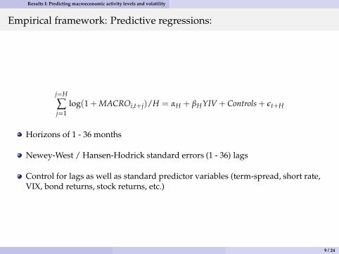
Empirical framework: Predictive regressions:

j=H

∑j=1

log(1 + MACROi,t+j)/H = αH + βHYIV + Controls + ǫt+H

Horizons of 1 - 36 months

Newey-West / Hansen-Hodrick standard errors (1 - 36) lags

Control for lags as well as standard predictor variables (term-spread, short rate,VIX, bond returns, stock returns, etc.)

9 / 24


YIV predicts real activity:

Table: 4, A3, A4, A5, A6: Predicting real activity: Coefficient on YIV

H = 12 18 24 30 36

GDP -0.08∗∗∗ -0.07∗∗∗ -0.05∗∗∗ -0.05∗∗∗ -0.04∗∗∗

(-3.61) (-3.46) (-3.83) (-3.99) (-3.72)

R2 34.42 26.80 20.72 17.12 14.72

IND -0.17∗∗∗ -0.12∗∗∗ -0.09∗∗∗ -0.06∗∗∗ -0.05∗∗

(-2.90) (-2.61) (-2.66) (-2.48) (-2.00)

R2 32.13 20.47 11.75 7.20 4.87

CON -0.09∗∗∗ -0.07∗∗∗ -0.06∗∗∗ -0.05∗∗∗ -0.05∗∗∗

(-3.31) (-3.19) (-3.36) (-3.52) (-3.76)

R2 34.48 27.76 21.63 17.58 16.11

EMP -0.09∗∗∗ -0.08∗∗∗ -0.07∗∗∗ -0.05∗∗∗ -0.04∗∗∗

(-6.25) (-5.36) (-4.97) (-4.71) (-4.06)

R2 44.77 38.55 29.40 21.78 15.52

Notes: Dependent is year-on-year growth rate in the GDP, IND, CON, EMP; Controls include the term spread; changes inshort-rate; Treasury bond returns; Corporate bonds returns; Stock index returns; CBOE Volatility Index; Economic uncertainty

from Baker/Bloom/Davis (2015); Quarterly or monthly data, 1990 - 2016.

10 / 24


YIV predicts volatility of real activity:

Table: 5, A7, A8, A9, A10: Predicting GDP, IP, CON, EMP volatility: Coefficient on YIV

H = 12 18 24 30 36

GDP 0.25∗∗∗ 0.30∗∗∗ 0.30∗∗ 0.26∗∗ 0.20∗∗

(2.95) (2.71) (2.30) (2.12) (2.03)

R2 25.35 26.99 27.45 29.19 30.60

IND 0.82∗∗∗ 1.06∗∗∗ 1.14∗∗∗ 1.02∗∗∗ 0.82∗∗∗

(3.60) (3.31) (3.04) (2.84) (2.49)

R2 36.33 34.29 31.41 23.86 16.21

CON 0.28∗∗∗ 0.33∗∗∗ 0.33∗∗∗ 0.30∗∗∗ 0.26∗∗∗

(4.06) (3.37) (3.08) (2.90) (2.53)

R2 30.69 25.53 20.34 16.58 13.10

EMP 0.22∗∗∗ 0.26∗∗∗ 0.29∗∗∗ 0.29∗∗∗ 0.27∗∗∗

(5.04) (4.19) (3.74) (3.52) (3.13)

R2 35.48 29.74 24.36 20.34 16.47

Notes: Dependent is year-on-year volatility of IP, CON, EMP; Quarterly or monthly data, 1990 - 2016.

11 / 24


Results robust to a battery of tests:

Predict over short- and long-term

Not driven by variance risk premia

Using non-overlapping data

Excluding financial crisis

Out of sample forecasts

Obvious question: Why does this work so well?

12 / 24

Results II: YIV captures interest rate uncertainty

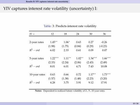
YIV captures interest rate volatility (uncertainty) I:

Table: 3: Predicts interest rate volatility

H = 12 18 24 30 36

2-year rates 1.45∗∗ 1.06∗ 0.63 0.27 -0.26

(1.98) (1.75) (0.84) (0.29) (-0.23)

R2− ord 6.02 2.33 0.61 0.09 0.07

5-year rates 1.22∗∗∗ 1.11∗∗ 1.02∗∗ 1.34∗∗∗ 1.66∗∗∗

(2.33) (2.24) (2.06) (2.43) (2.49)

R2− ord 8.01 6.01 4.71 7.43 10.08

10-year rates 0.63 0.66 0.72 1.17∗∗ 1.73∗∗∗

(1.57) (1.38) (1.48) (2.23) (3.20)

R2− ord 4.28 3.75 3.91 9.12 17.91

Notes: Dependent is realized future volatility of 2-, 5-, 10-year rates.

13 / 24

Results II: YIV captures interest rate uncertainty

YIV captures interest rate volatility (uncertainty) II:

Figure: 2: Response of YIV to monetary policy surprises

-2 -1 0 1 20.7590

0.8797

1.0003

1.1209

1.2416

1.3622Positive Surprises

-2 -1 0 1 20.7590

0.8797

1.0003

1.1209

1.2416

1.3622Negative Surprises

-2 -1 0 1 20.7590

0.8797

1.0003

1.1209

1.2416

1.3622No Surprises

YIV Short-rate VIX

Notes: YIV, the short rate, and the term spread over a 5-day window around Fed’s announcements regarding changes in the Federal Funds rate; Daily data,1990 - 2016.

YIV increases on both unexpected rate cuts and increases

14 / 24

Results III: Mechanism

Mechanism: YIV impacts real activity via bank balance sheets:

Figure: One possible mechanism

INTEREST

RATE

UNCERTAINTY

BANK

BALANCE

SHEETS

REAL

ACTIVITY

15 / 24


Bank centric view of interest rate risk:

Banks’ core activities deposits-taking and loans exposes their balance sheets tointerest rate risk

Banks cannot completely immunize themselves from interest rate uncertainty /risk

Interest rate uncertainty impacts bank liabilities → assets → net worth → realactivity

Drechsler/Savov/Schnabl (2017): Monetary policy affects real activity via bankdeposits

Haddad/Sraer (2017): Bank interest rate exposure forecasts bond returns

16 / 24


Support for our mechanism:

Evidence 1: YIV forecasts lower (higher) demand (volatility) for deposits frombanks

Evidence 2: YIV forecasts cost of capital of banks

Evidence 3: YIV forecasts level and volatility of bank credit

Evidence 4: Stronger forecasts for banks more exposed to IR risk

Evidence 5: YIV forecasts investment for bank dependent firms

17 / 24


Evidence 1: YIV and bank deposits:

Table: 6: Predicting bank deposits

H = 12 18 24 30 36

Bank deposit -0.25∗∗∗ -0.27∗∗∗ -0.28∗∗∗ -0.28∗∗∗ -0.29∗∗∗

(-3.31) (-4.19) (-4.70) (-4.66) (-4.36)

Bank deposit volatility 0.62∗∗∗ 0.45∗∗∗ 0.25∗ 0.18 0.12

(2.64) (2.68) (1.64) (0.98) (0.62)

Notes: Dependent is bank deposit growth and bank deposit volatility; Monthly data, 1990 - 2016.

18 / 24


Evidence 2: YIV and bank cost of capital:

Table: 7: Predicting bank cost of capital

H = 12 18 24 30 36

Libor-OIS spread 0.30∗∗ 0.24∗ 0.15 0.05 -0.07

(2.00) (1.82) (0.99) (0.28) (-0.29)

Bank E[R] 0.07 0.12 0.21∗ 0.27∗∗ 0.32∗∗

(1.06) (1.39) (1.87) (2.06) (2.25)Notes: Dependent is Libor-OIS spread or dividend yield on bank stocks or dividend yield for stock market; Monthly data, 1990 -

2016.

19 / 24


Evidence 3: YIV and bank credit:

Table: 8: Predicting bank credit

H = 12 18 24 30 36

Bank credit -0.13∗∗∗ -0.14∗∗∗ -0.14∗∗∗ -0.14∗∗∗ -0.14∗∗∗

(-3.07) (-4.30) (-4.42) (-4.51) (-5.06)

Bank credit volatility 0.61∗∗∗ 0.73∗∗∗ 0.60∗∗∗ 0.46∗∗∗ 0.33∗∗∗

(7.02) (5.47) (4.75) (4.51) (3.52)

Notes: Dependent is bank credit growth and bank credit volatility; Monthly data, 1990 - 2016.

20 / 24


Evidence 4: YIV and bank credit by exposure to IR risk:

Table: 9: Predicting bank credit by exposure to interest rate risk

H = 12 18 24 30 36

Small banks, Low Exp. -0.26∗∗∗ -0.28∗∗∗ -0.28∗∗∗ -0.28∗∗∗ -0.25∗∗∗

(-2.79) (-3.90) (-4.40) (-4.90) (-4.16)

Small banks, High Exp. -1.66∗∗ -1.99∗∗ -2.16∗∗ -2.36∗∗ -2.56∗∗

(-2.01) (-1.99) (-2.08) (-2.20) (-2.35)

Large banks, Low Exp. -0.18 -0.07 -0.01 -0.02 0.01

(-0.59) (-0.28) (-0.01) (-0.09) (0.03)

Large banks, High Exp. -0.31∗∗∗ -0.37∗∗∗ -0.39∗∗∗ -0.38∗∗∗ -0.35∗∗

(-2.59) (-2.76) (-2.60) (-2.46) (-2.16)

Notes: IR derivatives held for trading used to compute IR exposure (Purnanandam(2007)); Dependent is bank credit growth;Quarterly data, 1990 - 2016.

21 / 24


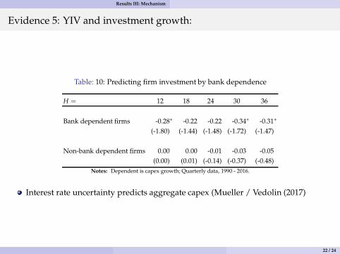
Evidence 5: YIV and investment growth:

Table: 10: Predicting firm investment by bank dependence

H = 12 18 24 30 36

Bank dependent firms -0.28∗ -0.22 -0.22 -0.34∗ -0.31∗

(-1.80) (-1.44) (-1.48) (-1.72) (-1.47)

Non-bank dependent firms 0.00 0.00 -0.01 -0.03 -0.05

(0.00) (0.01) (-0.14) (-0.37) (-0.48)

Notes: Dependent is capex growth; Quarterly data, 1990 - 2016.

Interest rate uncertainty predicts aggregate capex (Mueller / Vedolin (2017)

22 / 24

Conclusion

Key results:

I: A simple measure of uncertainty from Treasury derivatives markets predictslevel and volatility of macroeconomic activity

II: Over horizons of 1 - 36 months

III: Robust to a variety of specifications

23 / 24

Conclusion

Contribution:

Variable captures interest rate uncertainty

Directly impacts balance sheet of banks

Establish a link between time-varying uncertainty in US Treasury markets andbalance sheet of banks that impacts real activity

24 / 24

Documents

Treasury Yield Implied Volatility and Real Activity