Transverse Relaxation in Sandstones due to the eﬀect of

RICE UNIVERSITY

Transverse Relaxation in Sandstones due to the

effect of Internal Field Gradients and

Characterizing the pore structure of Vuggy

Carbonates using NMR and Tracer analysis

by

Neeraj Rohilla

A Thesis Submitted

in Partial Fulfillment of the

Requirements for the Degree

Doctor of Philosophy

Approved, Thesis Committee:

George J. Hirasaki, A. J. Hartsook Professor, ChairChemical and Biomolecular Engineering

Walter G. Chapman, William W. Akers ChairChemical and Biomolecular Engineering

Pedro Alvarez,George R. Brown Professor of EngineeringCivil and Environmental Engineering

Houston, Texas

February, 2013

Contents

List of Illustrations vi

List of Tables xv

Abstract 1

1 Introduction 4

2 Basic Principles and Literature Review 9

2.1 Basic Principles . . . . . . . . . . . . . . . . . . . . . . . . . . . . 9

2.1.1 Pulse tipping and Free Induction Decay . . . . . . . . . . . 10

2.1.2 Longitudinal (T1) Relaxation . . . . . . . . . . . . . . . . 11

2.1.3 Transverse (T2) Relaxation . . . . . . . . . . . . . . . . . 12

2.1.4 Diffusion-Induced Relaxation . . . . . . . . . . . . . . . . 14

2.1.5 Surface Relaxation and Pore size distribution . . . . . . . 15

2.2 Literature Review . . . . . . . . . . . . . . . . . . . . . . . . . . . 16

2.2.1 Diffusion Coupling . . . . . . . . . . . . . . . . . . . . . . 17

2.2.2 Inhomogeneities of the applied magnetic field . . . . . . . 20

2.2.3 Un-restricted or Free Diffusion . . . . . . . . . . . . . . . . 21

iii

2.2.4 Restricted Diffusion . . . . . . . . . . . . . . . . . . . . . . 25

2.3 Clay minerals in sandstones . . . . . . . . . . . . . . . . . . . . . 29

2.3.1 Formation of clay minerals in sandstones . . . . . . . . . . 30

2.3.2 Morphology of authigenic clays . . . . . . . . . . . . . . . 31

2.3.3 Effect of grain coating chlorite on formation evaluation . . 36

3 Modeling Internal Field Gradients in clay-lined sand-

stones 40

3.1 Simulations for FID and CPMG pulse sequence . . . . . . . . . . 48

3.1.1 Governing equations . . . . . . . . . . . . . . . . . . . . . 48

3.1.2 Boundary and Initial conditions . . . . . . . . . . . . . . . 49

3.2 Dimensionless groups and their significance . . . . . . . . . . . . . 50

3.3 FID results and discussion . . . . . . . . . . . . . . . . . . . . . . 53

3.4 CPMG results and discussion . . . . . . . . . . . . . . . . . . . . 56

3.5 Simulations for other geometrical parameters . . . . . . . . . . . . 68

3.6 Conclusions . . . . . . . . . . . . . . . . . . . . . . . . . . . . . . 73

4 Characterization of pore structure in vuggy carbon-

ates 74

4.1 NMR Experiments . . . . . . . . . . . . . . . . . . . . . . . . . . 78

4.2 NMR T2 Relaxation and pore size distribution . . . . . . . . . . . 79

iv

4.3 Calculating specific surface area of the rock from NMR T2

distribution . . . . . . . . . . . . . . . . . . . . . . . . . . . . . . 88

4.4 Tracer Analysis . . . . . . . . . . . . . . . . . . . . . . . . . . . . 92

4.5 Recovery Efficiency and Transfer Between Flowing And Stagnant

Streams . . . . . . . . . . . . . . . . . . . . . . . . . . . . . . . . 98

4.6 Parameter estimation from experimental data of tracer

concentration . . . . . . . . . . . . . . . . . . . . . . . . . . . . . 99

4.7 Setup for the Tracer flow experiments and the data acquisition

protocol . . . . . . . . . . . . . . . . . . . . . . . . . . . . . . . . 100

4.7.1 Reproducibility of tracer floods on core samples . . . . . . 101

4.8 Tracer Flow Experiments . . . . . . . . . . . . . . . . . . . . . . . 102

4.8.1 Validation with sandpacks and homogeneous rock system . 102

4.9 Characterization of heterogeneous samples . . . . . . . . . . . . . 103

4.9.1 Tracer flow experiments on 1.5 inch diameter samples . . . 104

4.10 Flow experiments on full sized cores . . . . . . . . . . . . . . . . . 118

4.11 Static and Dynamic adsorption of surfactant . . . . . . . . . . . . 125

4.11.1 Static adsorption of surfactant on the crushed rock powder 126

4.11.2 Dynamic adsorption of the surfactant on the rock surface . 128

5 Conclusions and Future Work 133

5.1 Conclusions . . . . . . . . . . . . . . . . . . . . . . . . . . . . . . 133

v

5.1.1 Modeling internal field gradients for claylined pores . . . . 133

5.2 Pore structure of vuggy carbonates . . . . . . . . . . . . . . . . . 134

5.2.1 NMR Chracterization . . . . . . . . . . . . . . . . . . . . . 134

5.2.2 Characterization of the pore space by Tracer Analysis . . . 135

5.3 Future Work . . . . . . . . . . . . . . . . . . . . . . . . . . . . . . 136

5.3.1 Dynamic adsorption model for heterogeneous systems . . . 136

A Manual on using bromide ion sensitive electrode in

laboratory experiments 139

Bibliography 153

Illustrations

2.1 Chlorite coating inhibiting quartz overgrowth . . . . . . . . . . . 30

2.2 (A) Stacked plates of kaolinite in porous sandstone (face-to-face

arrangement and pseudohexagonal outlines of individual plates)

(B) Vermicular authigenic kaolinite in porous sandstone . . . . . 32

2.3 SEM image of illite, showing lath-like projections which extend

from one grain to another . . . . . . . . . . . . . . . . . . . . . . 33

2.4 SEM image of illite, showing delicate fiber like structure . . . . . 34

2.5 SEM images of grain coating chlorite at different magnifications.

The images on left and right are at 50 and 400 magnifications

respectively . . . . . . . . . . . . . . . . . . . . . . . . . . . . . . 34

2.6 SEM images of grain coating chlorite at different magnifications.

The images on left and right are at 1,000 and 10,000

magnifications respectively . . . . . . . . . . . . . . . . . . . . . 35

2.7 Chlorite clay exhibiting delicate rosette like morphology . . . . . 35

2.8 Field lines for the induced magnetic field for a clay lined macropore 38

vii

2.9 Contours of dimensionless magnetic field gradient for a claylined

macropore . . . . . . . . . . . . . . . . . . . . . . . . . . . . . . 39

3.1 T1 and T2 relaxation time spectrum for North Burbank core

sample saturated with brine solution . . . . . . . . . . . . . . . . 41

3.2 Schematic of a macropore lined with clay flakes . . . . . . . . . . 42

3.3 Schematic of a clay-lined pore . . . . . . . . . . . . . . . . . . . . 43

3.4 Schematic of the simulation domain . . . . . . . . . . . . . . . . . 44

3.5 (a) Field lines of the total magnetic field B due to the clay flake

in a homogeneous field B0 (b) Field lines of the induced magnetic

field Bδ due to the clay flake in a homogeneous field B0 . . . . . . 45

3.6 (a) Contour lines of the z component of induced field (b)

Contours of dimensionless gradient due to the presence of clay flake 45

3.7 Schematic of mesh used to resolve large values of gradients

around the corner . . . . . . . . . . . . . . . . . . . . . . . . . . . 47

3.8 Decay of the magnitude of magnetic moment versus

dimensionless time for different value of ζ= τRτω

. . . . . . . . . . . 54

3.9 Comparison of FID decay of magnetization for different values of

ζ = τRτω

and for the case when no diffusion is present . . . . . . . . 56

viii

3.10 Plot for CPMG decay of magnitude of magnetization for

dimensionless echo spacing, δωτE = 5.0 and ζ = δωτR = 100.

Geometrical parameters used are: aspect ratio of macropore (η)

= 1, aspect ratio of the clay flake (λ) = 1 and microporosity

fraction (β) = 0.5 . . . . . . . . . . . . . . . . . . . . . . . . . . . 57

3.11 Bi-exponential plot for ζ = 2681, τ ∗E=20.0 . . . . . . . . . . . . . 59



3.14 Representation of different relaxation regimes as function of three

timescales . . . . . . . . . . . . . . . . . . . . . . . . . . . . . . . 61

3.15 A plot of secular relaxation rate versus δωτR for different values

of dimensionless half-echo spacing (δωτE). Geometrical

parameters used are: aspect ratio of macropore (η) = 1, aspect

ratio of the clay flake (λ) = 1 and microporosity fraction (β) = 0.5 64

3.16 Plot of secular relaxation rate as function of δωτE for different

values of δωτR. Geometrical parameters used are: aspect ratio of

macropore (η) = 1, aspect ratio of the clay flake (λ) = 1 and

microporosity fraction (β) = 0.5 . . . . . . . . . . . . . . . . . . . 65

3.17 Plot of secular relaxation rate as function of δωτE for different

values of δωτR demonstrating various echo-spacing dependence in

different regimes . . . . . . . . . . . . . . . . . . . . . . . . . . . . 66

ix

3.18 Contours of secular relaxation rate as a function of δωτR for

different values of δωτE. Geometrical parameters used are:

aspect ratio of macropore (η) = 1, aspect ratio of the clay flake

(λ) = 1 and microporosity fraction (β) = 0.5 . . . . . . . . . . . . 67

















x

4.1 Core ID-1; Length = 9.0 inches, Diameter = 3.5 inches;

Fractured, low porosity, No apparent vugs, uniform cylindrical

shape . . . . . . . . . . . . . . . . . . . . . . . . . . . . . . . . . . 75

4.2 Core ID-2; Length = 5.5 inches, Diameter = 3.5 inches; Vuggy,

well cored, uniform cylindrical shape . . . . . . . . . . . . . . . . 76

4.3 Core ID-3; Length = 3.5, 6 inches, Diameter = 3.5 inches; Very

vuggy, well cored, uniform cylindrical shape . . . . . . . . . . . . 76

4.4 Core ID-4; Length = 4 inches, Diameter = 4.0 inches; Some big

vugs, well cored . . . . . . . . . . . . . . . . . . . . . . . . . . . . 77

4.5 Core ID-5; Length = 4.0 inches, Diameter = 4.0 inches; Breccia,

very vuggy and heterogeneous . . . . . . . . . . . . . . . . . . . . 77

4.6 A comparison of before (shown at left) and after (shown at right)

cleaned pictures for a core-plug (Plug ID: 3V) . . . . . . . . . . . 80

4.7 A comparison of before (shown at left) and after (shown at right)

cleaned pictures for a core-plug (Plug ID: 2V) . . . . . . . . . . . 81

4.8 T2 relaxation time spectrum for 100 % brine saturated core-plug

(Plug ID: 3V) . . . . . . . . . . . . . . . . . . . . . . . . . . . . . 83


(Plug ID: 2V) . . . . . . . . . . . . . . . . . . . . . . . . . . . . . 84


(Plug ID: 2VA) . . . . . . . . . . . . . . . . . . . . . . . . . . . . 84

xi


(Plug ID: 1H) . . . . . . . . . . . . . . . . . . . . . . . . . . . . . 85


(Plug ID: 1HA) . . . . . . . . . . . . . . . . . . . . . . . . . . . . 85

4.13 Permeability versus T2 Log mean for various core samples . . . . . 86

4.14 Permeability versus T2 Log mean while using T2 cut off of 750

msec for various core samples . . . . . . . . . . . . . . . . . . . . 87

4.15 T2 relaxation time and S/V spectrum for 100 % brine saturated

core-plug (Plug ID: 1H) . . . . . . . . . . . . . . . . . . . . . . . 90

4.16 T2 relaxation time spectrum for 100 % brine saturated crushed

rock powder . . . . . . . . . . . . . . . . . . . . . . . . . . . . . . 91

4.17 A bar chart for the specific surface area of several core plugs . . . 91

4.18 Schematic of the pore system containing interconnect flow

channels, touching/isolated vugs and stagnant/dead end pores . . 92

4.19 Effluent concentration versus pore volume throughput for a set of

dimensionless parameters . . . . . . . . . . . . . . . . . . . . . . . 97

4.20 Plots of effluent concentration and recovery efficiency as a

function of pore volume throughput illustrating importance of

mass transfer between flowing and stagnant streams . . . . . . . . 108

4.21 A comparison of synthetic data with and without noise used for

benchmarking parameter estimation algorithm . . . . . . . . . . . 109

xii

4.22 A comparison of transfer function for experimental data and

fitted curve for parameter estimation . . . . . . . . . . . . . . . . 109

4.23 Comparison of fitted model parameters using the inversion

routine when (A) Data at one flowrate is used and (B) When

data at two flow rates is used . . . . . . . . . . . . . . . . . . . . 110

4.24 Effluent concentration versus pore volume throughput for 100

ppm and 10,000 ppm floods for similar values of the flowrates . . 111

4.25 Effluent concentration versus pore volume throughput for 100

ppm and 10,000 ppm floods for several values of the flowrates . . 111

4.26 Effluent concentration versus pore volume throughput for

homogeneous and heterogeneous sandpacks . . . . . . . . . . . . . 112

4.27 Effluent concentration and Recovery efficiency as a function of

pore volume for homogeneous Silurian outcrop sample . . . . . . . 113

4.28 (A) Transfer function for the fitted parameters (B) Effluent

concentration and recovery efficiency for core plug 3V (diameter

= 1.5 inch, length = 1.25 inch) at the flow rate of 15 ft/day and

(C) The corresponding NMR T2 distribution for the core plug 3V 114

4.29 (A) Transfer function for fitted parameters (B) Effluent

concentration and recovery efficiency for core plug 1H (diameter

= 1.5 inch, length = 2.25 inch) at the flow rate of 1.4 ft/day and

(C) The corresponding NMR T2 distribution for the core plug 1H 115

xiii

4.30 ((A) Transfer function for the fitted parameters (B) Effluent

concentration and recovery efficiency for core plug 1.5D

(diameter = 1.5 inch, length = 3 inch), (C) The corresponding

NMR T2 distribution for the core plug 1.5D . . . . . . . . . . . . 116

4.31 (A) Transfer function for the fitted parameters (B) Effluent

concentration and recovery efficiency for core plug 1.5C (diameter

= 1.5 inch, length = 3.5 inch), (C) The corresponding NMR T2

distribution for the core plug 1.5B . . . . . . . . . . . . . . . . . . 117

4.32 Transfer functions for the fitted parameters for 3.5B, 3.5C and

3.5D rock samples . . . . . . . . . . . . . . . . . . . . . . . . . . . 120

4.33 Effluent concentration and Recovery efficiency for the cases when

strong mass transfer is observed. (A) Sample 3.5D with 1/M =

0.6 days and (B) Sample 4.0B with 1/M = 0.1 days . . . . . . . . 121

4.34 Effluent concentration and Recovery efficiency for the cases when

mass transfer is small. (A) Sample 3.5C with 1/M = 2.1 days

and (B) Sample 3.5B with 1/M = 4.3days . . . . . . . . . . . . . 122

4.35 Calculated Effluent concentration and Recovery Efficiency for

various interstitial velocities using parameters estimated from

tracer flow experiments . . . . . . . . . . . . . . . . . . . . . . . . 124

4.36 Adsorption on NI blend on crushed powder rock with BET area

of 1.5 m2/gm . . . . . . . . . . . . . . . . . . . . . . . . . . . . . 127

xiv

4.37 Adsorption of NI blend on a heterogeneous rock sample (A)

Comparison of the surfactant fast flood with tracer (B)

Comparison of the slow surfactant flood with tracer . . . . . . . . 130

4.38 A comparison of fast and slow surfactant floods showing

adsorption of NI blend on a heterogeneous rock sample . . . . . . 131

Tables

4.1 Comparison of porosity for different core-plugs . . . . . . . . . . . 80

4.2 Summary of estimated model parameters from various tracer flow

experiments for 1.5 inch diameter core samples . . . . . . . . . . . 107

4.3 Summary of estimated model parameters from various tracer flow

experiments for full core samples . . . . . . . . . . . . . . . . . . 125

4.4 Summary of both surfactant flood and loss of surfactant due to

dynamic adsorption . . . . . . . . . . . . . . . . . . . . . . . . . . 132

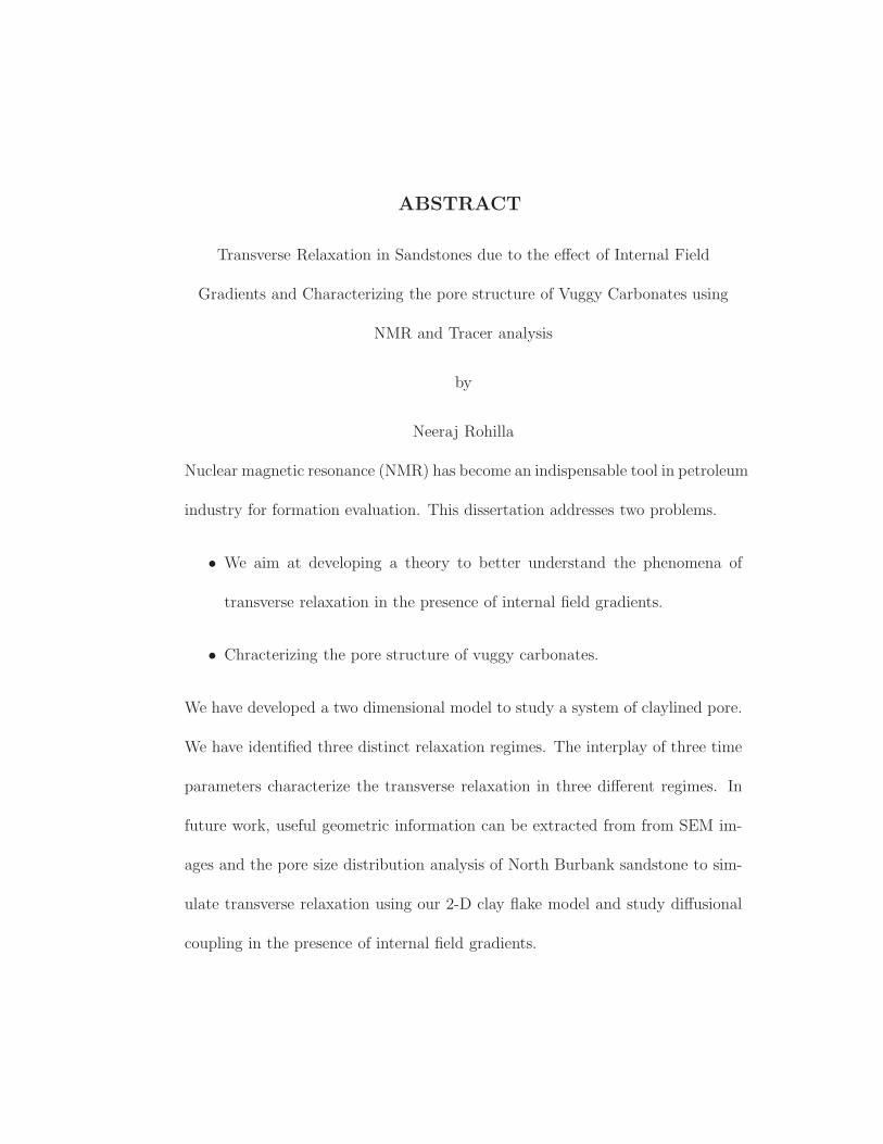
ABSTRACT

Transverse Relaxation in Sandstones due to the effect of Internal Field

Gradients and Characterizing the pore structure of Vuggy Carbonates using

NMR and Tracer analysis

by

Neeraj Rohilla

Nuclear magnetic resonance (NMR) has become an indispensable tool in petroleum

industry for formation evaluation. This dissertation addresses two problems.

• We aim at developing a theory to better understand the phenomena of

transverse relaxation in the presence of internal field gradients.

• Chracterizing the pore structure of vuggy carbonates.

We have developed a two dimensional model to study a system of claylined pore.

We have identified three distinct relaxation regimes. The interplay of three time

parameters characterize the transverse relaxation in three different regimes. In

future work, useful geometric information can be extracted from from SEM im-

ages and the pore size distribution analysis of North Burbank sandstone to sim-

ulate transverse relaxation using our 2-D clay flake model and study diffusional

coupling in the presence of internal field gradients.

2

Carbonates reservoirs exhibit complex pore structure with micropores and

macropores/vugs. Vuggy pore space can be divided into separate-vugs and

touching-vugs, depending on vug interconnection. Separate vugs are connected

only through interparticle pore networks and do not contribute to permeability.

Touching vugs are independent of rock fabric and form an interconnected pore

system enhancing the permeability. Accurate characterization of pore structure

of carbonate reservoirs is essential for design and implementation of enhanced

oil recovery processes. However, characterizing pore structure in carbonates is

a complex task due to the diverse variety of pore types seen in carbonates and

extreme pore level heterogeneity. The carbonate samples which are focus of this

study are very heterogeneous in pore structures. Some of the sample rocks are

breccia and other samples are fractured. In order to characterize the pore size in

vuggy carbonates, we use NMR along with tracer analysis. The distribution of

porosity between micro and macro-porosity can be measured by NMR. However,

NMR cannot predict if different sized vugs are connected or isolated. Tracer

analysis is used to characterize the connectivity of the vug system and matrix.

Modified version of differential capacitance model of Coats and Smith (1964) and

a solution procedure developed by Baker (1975) is used to study dispersion and

capacitance effects in core-samples. The model has three dimensionless groups:

1) flowing fraction (f), 2) dimensionless group for mass transfer (NM) character-

izing the mass transfer between flowing and stagnant phase and 3) dimensionless

3

group for dispersion (NK) characterizing the extent of dispersion. In order to ob-

tain unique set of model parameters from experimental data, we have developed

an algorithm which uses effluent concentration data at two different flow rates to

obtain the fitted parameter for both cases simultaneously. Tracer analysis gives

valuable insight on fraction of dead-end pores and dispersion and mass transfer

effects at core scale. This can be used to model the flow of surfactant solution

through vuggy and fractured carbonates to evaluate the loss of surfactant due to

dynamic adsorption.

4

Chapter 1

Introduction

The ever increasing demand for energy worldwide is calling for accurate and so-

phisticated methods for evaluating petroleum formations. These approaches in-

clude seismic data analysis, various logging methods (such as wireline, acoustic,

neutron density, gamma ray and nuclear magnetic resonance) and core analysis

in laboratory. Nuclear magnetic resonance (NMR) has increasingly become an

indispensable tool in the field of petroleum technology due to its numerous ap-

plications. NMR is applied for measurements of porosity, pore size distribution,

permeability, viscosity, diffusion coefficient, residual oil and water saturation and

free-fluid index (Kenyon 1997). The difference in NMR properties of different

fluids is used as a basis for pore fluid identification. Different techniques based

on Longitudinal (T1) and Transverse (T2) relaxation measurements are used for

evaluating formation properties and reservoir fluid properties.

The estimation of bulk volume irreducible (BVI), free-fluid index (FFI), per-

meability and fluid type relies on the accurate interpretation of T1 and T2 relax-

ation. The NMR response in porous media is complicated due to various factors.

The first of these is diffusional coupling between macropore and micropore. Fluid

5

molecules relax at the micropore surface and if the diffusion is fast (i.e. relax-

ation at the micropore surface is much slower compared to diffusional transport

of molecules to the pore surface), whole pore relaxes at a single T2. Traditional

methods for the interpretation of NMR data use the assumption of fast diffusion.

However, if the surface relaxation is very fast or diffusion is slow, the diffusion

is not sufficient to homogenize the relaxing molecules and both micro and macro

pore decay at different T2 (Anand and Hirasaki 2007a). In such cases, traditional

methods to calculate free-fluid index like sharp cut off may give erroneous results

(Straley, Morriss, Kenyon and Howard 1991). The extent of diffusional coupling

and its effect on relaxation time spectrum is quantitatively analyzed by Anand

and Hirasaki (2007a).

Inhomogeneities in the applied magnetic field significantly affect transverse

relaxation. Magnetic field inhomogeneities can be either externally applied (by

the logging tool) or internal field gradients. The applied magnetic field by the log-

ging tool is only uniform near the center of the coils (Tarczon and Halperin 1985).

Thus much of the sample volume could be exposed to a non-uniform magnetic

field. Internal field gradients in the pore space are caused by the susceptibility

contrast between solid matrix and the fluid filling the pore space. It is commonly

assumed that these field gradients are caused by paramagnetic minerals such as

iron, nickel or manganese which are frequently found in clays (Kleinberg, Kenyon

and Mitra 1994).

6

Laboratory or field diffusion measurements by default assume that the spins

can diffuse freely. This means that distribution of spins is Gaussian and that

the diffusion is not limited by geometrical constraints. This is only true when

diffusion length (ld =√Dτ) is smaller than the dephasing length (lg = (Dγg)1/3)

and the size of the pore (ls = V/S). Only in such instances, the formula of free

diffusion regime developed by Neuman (1974) can be applied. When internal field

gradients are higher or comparable to those applied by the logging tools, the use

of free diffusion formula can overestimate the value of diffusion coefficient due to

enhanced relaxation. In such cases, the diffusion based interpretation techniques

for pore fluid identification could lead to erroneous results.

Another important consideration is that of restricted diffusion due to geo-

metrical restrictions. At times short enough that most spins do not encounter

the pore walls or experience a significant change in local gradient, we expect the

protons to behave as if they are a part of infinite fluid medium. If the size of

geometrical confinement is smaller than the diffusion length (√Dτ), the diffu-

sion measurements are strongly affected by surface relaxation and the local field

gradient resulting in a time-dependent value of effective diffusion coefficient.

In sedimentary rocks, a detailed understanding of transverse relaxation is

not only the function of susceptibility contrast but also of the pore geometry.

Hence, an accurate interpretation of transverse relaxation in principle, can give

valuable insights about the pore fluid and the pore structure. In recent years,

7

the researchers have attempted to use the internal field gradients as a convenient

way to deduce information about the micro-geometry of the formation such as

pore connectivity, isolated pores and pore structure using the concept of decay

due to diffusion in the internal field (DDIF) (Mitra and Sen 1992, Song et al.

2000, Song 2000, Song 2001, Chen and Song 2002, Song et al. 2002).

The interpretation of transverse relaxation is complicated when effects of spins

self-diffusion in an inhomogeneous field and restricted geometry become domi-

nant. So far, only simple cases of magnetic field inhomogeneities (linear, parabolic

and cosine) have been taken into account in the context of restricted diffusion

(Le Doussal and Sen 1992a, Grebenkov 2007). The combined effects of diffusion

coupling, restricted diffusion and internal field gradients are not completely un-

derstood. A detailed understanding of combined effect of these phenomena will

serve as a tool to better interpret NMR wells logs and enable us to accurately

evaluate petroleum formations.

The second part of this study deals with charactering vuggy carbonates. Car-

bonates account for more than 50 % of the world’s hydrocarbons reserves (Palaz

and Marfurt 1997). Carbonate formation exhibit wide range of pore sizes and

types (Lucia 1999). Many carbonates are triple porosity system where the poros-

ity is distributed among micro-pores, marco-pores and large vugs. Such hetero-

geneities come in variety of length scales from microscopic to macroscopic level.

Therefore predicting the properties of a carbonate reservoir on a field scale is

8

extremely difficult. Understanding the pore structure of such carbonate systems

is very essential for designing and implementation of enhanced oil recovery pro-

cesses. We use laboratory NMR experiments along with tracer flow analysis to

characterize the pore structure of carbonates. Hidajat, Mohanty, Flaum and Hi-

rasaki (2004) studied vuggy carbonate samples using core analysis, NMR and

X-ray CT scanning. They found that for vuggy carbonates CT scans and tracer

effluent concentration profiles can help identify the preferential flow paths and

the variation of the porosity within the cores.

This thesis is organized as follows. In chapter two we briefly review the rel-

evant literature for transverse relaxation in the presence of diffusion with and

without geometrical restriction and effect of grain-coating chlorite clay on trans-

verse relaxation. Chapter three describes a two dimensional model to describe

transverse relaxation in chlorite coated sandstones like North Burbank sandstone.

Chapter four describe the NMR and tracer analysis for characterizing the pore

structure in vuggy carbonates. Chapter five describes future scope of this work.

9

Chapter 2

Basic Principles and Literature Review

In this chapter we describe the basic principles of NMR and a brief literature

review on the subject of internal field gradients. Later, relevant modeling ap-

proaches will be discusses in detail to outline the scope of present work.

2.1 Basic Principles

NMR loosely refers to the phenomena of behavior of atomic nuclei under the

influence of externally applied magnetic fields. If the spins of protons and/or

neutrons in a nucleus are paired, the overall spin of the nucleus is zero. When

the spins of protons and/or neutrons are not paired, the overall spin of the nu-

cleus generates a magnetic moment along the spin axis. NMR measurements

can be made on any nucleus that has an odd number of protons or neutrons or

both, such as the nucleus of hydrogen (1H), carbon (13C), and sodium (23Na) etc.

NMR studies presented in this work are based on responses of the nucleus of the

hydrogen atom.

Under the influence of an externally applied magnetic field, B0, the individual

magnetic moments align parallel (lower energy state) or antiparallel (higher en-

10

ergy state) to the field. There is slight preference of nuclei for aligning parallel to

the applied field which gives rise to a net magnetization (M0) along the direction

of applied field.

The external magnetic field (B0) produces a torque on the magnetic moment.

If the external field is static, it causes magnetic moment to precess about the

applied field at a fixed angle. The equation of motion for the macroscopic mag-

netization (M) is given by equating the torque due to the external field with the

rate of change of M shown below.

dM

dt= M × (γB0) (2.1)

Where γ is gyromagnetic ratio, which is a measure of the strength of the nuclear

magnetism. The frequency for the precession of magnetic moment about applied

field is called Larmor frequency and is given by:

f =γB0

2π(2.2)

2.1.1 Pulse tipping and Free Induction Decay

The magnetization (M) remains in equilibrium state until perturbed. If the

static magnetic field is in the longitudinal direction and a magnetic field rotating

at Larmor frequency is applied in the plane perpendicular to the static field, the

11

magnetization starts to tip from the longitudinal direction towards transverse

plane. The angle θ through which the magnetization is tipped is given as:

θp = γB1tp (2.3)

Where tp is the time over which the oscillating field is applied and B1 is the

amplitude of the applied magnetic field. In NMR measurements, usually a π

(θp = 1800) or π2(θp = 900) radio frequency (RF) pulse is applied. When the RF

pulse is removed, the relaxation mechanisms cause the magnetization to return

to equilibrium condition. If a coil of wire is set up around the axis perpendicular

to Bo, oscillations of M induces a sinusoidal current in the coil which can be

detected. This signal is called the Free Induction Decay (FID).

2.1.2 Longitudinal (T1) Relaxation

Longitudinal relaxation is also called spin-lattice relaxation. In the absence of an

external magnetic field, protons do not align in any preferred direction and the

net magnetization is zero. When the external field is applied, protons respond to

this field and net magnetization begins to build up. The time constant for this

first order kinetic process is called T1. The equation describing the longitudinal

relaxation is given as:

dMz

dt= − [Mz −M0]

T1

(2.4)

12

Where, M0 is the equilibrium magnetization and Mz is the z component of mag-

netization. A common pulse sequence used to measure T1 relaxation time is the

Inversion-Recovery (IR) pulse sequence. The IR sequence starts with a 1800 pulse

which flips the magnetization in the negative z direction. After a fixed amount

of time t, a 900 pulse is applied which brings the magnetization to the x − y

plane. Free induction decay of the magnetization after the 900 pulse induces a

sinusoidal voltage which is detected by the receiver coil. The amplitude of the

FID immediately after the 900 pulse gives the value of Mz after the wait time

t. A series of such experiments are performed for a range of values of t, which

give the values of Mz increasing from -M0 to +M0. The T1 relaxation time is

determined by fitting an exponential fit to the measured values of Mz given as

Mz(t) = M0

(

1− 2 exp

(−t

T1

))

(2.5)

2.1.3 Transverse (T2) Relaxation

Transverse relaxation is also called spin-spin relaxation. When a 900 pulse is

applied, all the spins are in transverse plane. After the application of a 900 pulse,

the proton population begins to dephase, or lose phase coherency. This means

that the precession of the protons will no longer be in phase with one another.

As dephasing progresses, the net magnetization decreases. This decay is usually

exponential and is characterized by the FID time constant (T ∗

2 ). FID is caused by

13

certain molecular relaxation processes and due to magnetic field inhomogeneities.

The equation describing transverse relaxation is given as:

dMx,y

dt= −Mx,y

T ∗

2

(2.6)

1

T ∗

2

=1

T2

+ γ∆B0 (2.7)

Where ∆B0 is the inhomogeneity of the magnetic field.

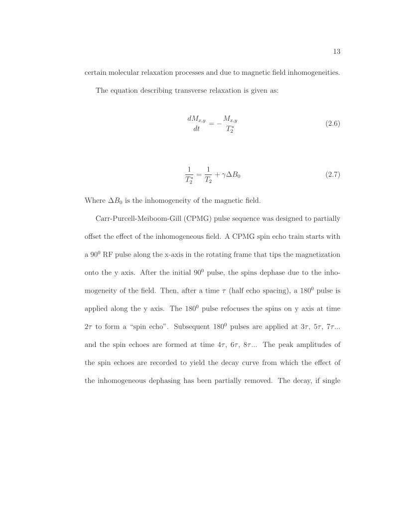
Carr-Purcell-Meiboom-Gill (CPMG) pulse sequence was designed to partially

offset the effect of the inhomogeneous field. A CPMG spin echo train starts with

a 900 RF pulse along the x-axis in the rotating frame that tips the magnetization

onto the y axis. After the initial 900 pulse, the spins dephase due to the inho-

mogeneity of the field. Then, after a time τ (half echo spacing), a 1800 pulse is

applied along the y axis. The 1800 pulse refocuses the spins on y axis at time

2τ to form a “spin echo”. Subsequent 1800 pulses are applied at 3τ , 5τ , 7τ ...

and the spin echoes are formed at time 4τ , 6τ , 8τ ... The peak amplitudes of

the spin echoes are recorded to yield the decay curve from which the effect of

the inhomogeneous dephasing has been partially removed. The decay, if single

14

exponential, can be expressed as:

Mx,y(t) = M0 exp

(

− t

T2

)

(2.8)

Where, t = [2τ, 4τ, 6τ...].

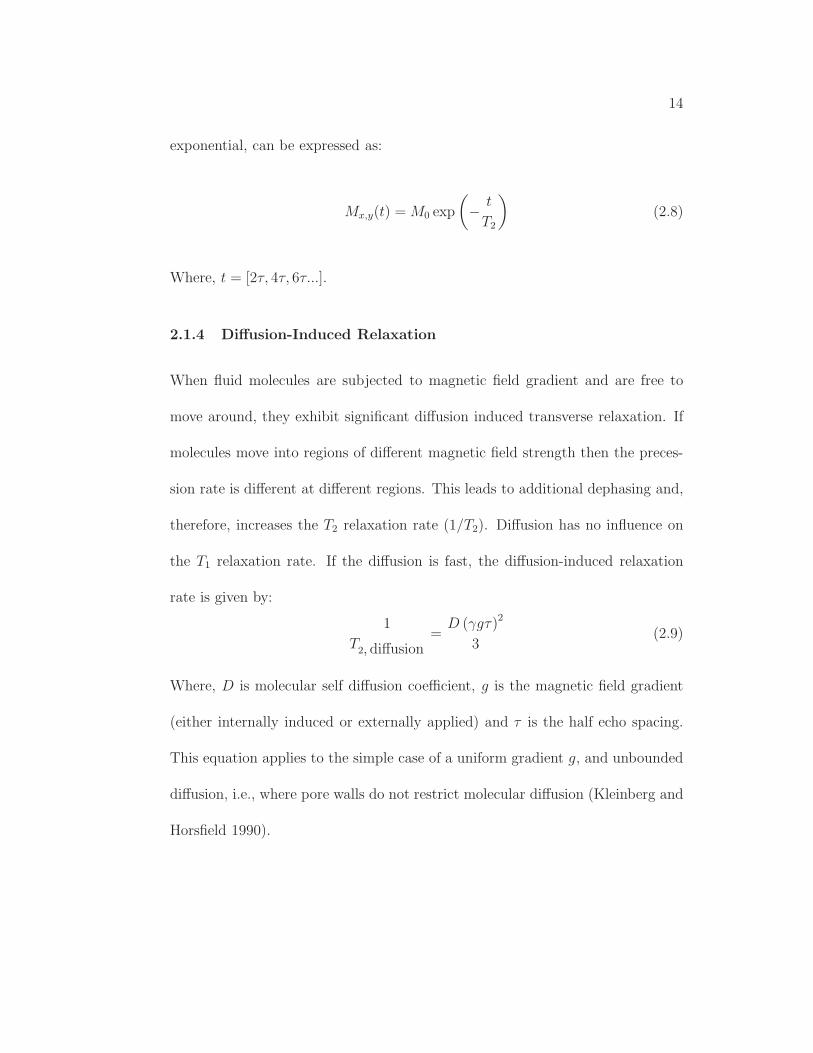
2.1.4 Diffusion-Induced Relaxation

When fluid molecules are subjected to magnetic field gradient and are free to

move around, they exhibit significant diffusion induced transverse relaxation. If

molecules move into regions of different magnetic field strength then the preces-

sion rate is different at different regions. This leads to additional dephasing and,

therefore, increases the T2 relaxation rate (1/T2). Diffusion has no influence on

the T1 relaxation rate. If the diffusion is fast, the diffusion-induced relaxation

rate is given by:

1

T2, diffusion

=D (γgτ)2

3(2.9)

Where, D is molecular self diffusion coefficient, g is the magnetic field gradient

(either internally induced or externally applied) and τ is the half echo spacing.

This equation applies to the simple case of a uniform gradient g, and unbounded

diffusion, i.e., where pore walls do not restrict molecular diffusion (Kleinberg and

Horsfield 1990).

15

2.1.5 Surface Relaxation and Pore size distribution

The NMR response of protons in pore space of the rocks is significantly different

than that in the bulk due to interactions with the pore surface. Surface relaxation

occurs at the fluid-solid interface, i.e. at the grain surface of rocks. In the

limit of fast diffusion (i.e. relaxation at the surface of the pores is much slower

compared to the transport of spins to the pore surface), the surface relaxation is

characterized by surface relaxivities (ρ1 and ρ2) for longitudinal and transverse

relaxation, and surface to volume (S/V ) ratio of the pores (Brownstein and Tarr

1979).

1

T1, surface

= ρ1

(

S

V

)

pore(2.10)

1

T2, surface

= ρ2

(

S

V

)

pore(2.11)

Surface relaxivity varies with mineralogy. Carbonate formations exhibit weaker

surface relaxivity than quartz surface.

For a rock sample having a pore size distribution, in the limit of fast diffusion

all pores relax independent of each other. Each pore size is associated with a

T2 component and the net magnetization will no longer relax as a single expo-

nential, but instead, relax as a multi-exponential decay. Thus, the observed T2

distribution of all the pores in the system represents the pore size distribution of

16

the rock sample (Loren and Robinson 1970, Brownstein and Tarr 1979).

Relaxation mechanisms act in parallel and, therefore, the relaxation rates can

be written as:

1

T1

=1

T1, bulk

+1

T1, surface

(2.12)

1

T2

=1

T2, bulk

+1

T2, surface

+1

T2, diffusion

(2.13)

2.2 Literature Review

Nuclear Magnetic Resonance (NMR) and Magnetic Resonance Imaging (MRI) are

frequently used in petrophysics and in the field of medicine. Petrophysics and

the field of medicine share some key problems for NMR/MRI. In medicine, the

objective is to construct a sharp and accurate image for distinguishing between

different types of tissues, bones and body fluids, all having different magnetic

susceptibility. Sometimes in MRI, the contrasting agents containing paramag-

netic particles are deliberately injected into the body to obtain a high resolution

image. On the other hand in petrophysics, the object of interest is a rock sam-

ple or petroleum formation which has different magnetic susceptibility than the

susceptibility of pore filling fluid.

In this section we summarize the key research contributions for diffusion cou-

pling and understanding transverse relaxation in the presence of inhomogeneous

17

magnetic field. We also point out their key assumptions and limitations which

will provide the motivation for the current work.

2.2.1 Diffusion Coupling

As described in section 2.1.5, pore size estimation from NMR measurements on

fluid saturated porous media assumes that the T2 distribution is directly related to

the pore size distribution and the net magnetization decays as a multiexponential

decay.

M(t) =∑

i

fi exp

(

− t

T2,i

)

(2.14)

where fi is the amplitude of each T2,i. Such interpretation assumes that different

pores relax independent of each other. However, when surface relaxation is very

fast or diffusion is slow, this assumption breaks down and fluid molecules in

different sized pore communicate with each other through diffusion. This is true

for the case of rocks where porosity is divided between two or more populations

of very different length scales.

Ramakrishnan et al. (1999) observed that NMR T2 measurements on water

saturated peloidal grainstone exhibit a single peak suggesting a single pore size.

However, the ESEM images of the sample showed a wide range of pore sizes ex-

hibiting both micro and macro porosities. Ramakrishnan et al. (1999) explained

this behavior using three-dimensional random walk simulations considering the

18

diffusion of fluid molecules between macro and micro pores. They proposed an

analytical model of 3D array of spherical micropores surrounded by intergranular

pores. This model can be simplied as two-dimensional periodic array of iden-

tial slab-like microporous grains separated by intergranular pores. This model

is completely described by four parameters total porosity, φ, volume fraction of

intergranular porosity, fm, the pore volume to surface area ratio for macrop-

ores, VSm and the pore volume to surface area ratio for micropores T2µ. They

found that when decay of magnetization in macropore happens on a much larger

timescale in comparison to that of micropore, the relaxation can be expressed

as a bi-exponential decay with amplitudes representing micro and macroporosity

fractions as shown in the equation below.

M(t) = (φ− fm) exp

(

− t

T2,µ

)

+ fm exp

(

− ρat

VSm

)

(2.15)

Where, VSm is the macropore volume-to-surface ratio, φ and fm are the total

porosity and macroporosity respectively and ρa is the apparent relaxivity for the

macropore. The above bi-exponential decay model is only valid when the diffusion

length within the microporous grain is much smaller than the grain radius, i.e.

√

DT2,µ

φµFµ<< Rg (2.16)

19

Where, Fµ is the formation factor.

Toumelin et al. (2003) used a conditional Monte Carlo random-walk algo-

rithm to simulation the NMR response for a three-dimensional array of spheres

of different sizes representing porous media. The three-dimensional model can

accomodate different pore sizes and can represent both micro and macroporosity.

The model allows diffusional coupling between different pore modes. The model

has four parameters, 1) average pore radii 2) porosities of different pore sizes 3)

micro-porosity radius and 4) surface relaxivity. First two parameters are obtained

by SEM analysis of core samples while other two are fitted to match simulation

results with NMR measurements in laboratory. By keeping the same parame-

ters and by preventing the diffusional coupling between pore modes, equivalent

uncoupled models are constructed. Simulations through these uncoupled models

yield the NMR response which would have been observed in laboratory in the

absence of diffusion coupling. These results can be used to calculate the extent of

diffusional coupling on estimation of BVI. They showed that in some cases using

a T2,cutoff of 90 ms for carbonates can results in substantial error of 48 % in BVI

calculations.

Anand and Hirasaki (2007a) explained diffusional coupling based on a cou-

pling parameter (α) for a clay lined pore (Straley, Morriss, Kenyon and Howard

1995). The coupling parameter (α) is the ratio of characteristic relaxation rate of

the pore to the rate of diffusional mixing of spins between the micro and macro-

20

pore. Depending on the value of coupling parameter (α), micro and macropores

can communicate through total, intermediate or decoupled regimes of coupling.

For values of α less than 1, the micropore is totally coupled with the macropore

and the entire pore relaxes with a single relaxation rate. In intermediate coupling

(1 < α < 250) regime, the T2 distribution consists of two distinct peaks for two

pore types but the peak amplitudes are not representative of micro and macro

porosity fractions. For values of α greater than 250, the two pores relax indepen-

dent of each other and T2 distribution correctly represents micro and macropore

relaxation and the peak amplitudes are representative of the porosity fractions (β

and 1− β for micro and macroporosity respectively). They also found appropri-

ate coupling parameter for grainstones using the spherical grain model developed

by Ramakrishnan et al. (1999). They developed a new technique for calculating

irreducible fluid saturation that is applicable in all coupling regimes.

2.2.2 Inhomogeneities of the applied magnetic field

Diffusion of fluid molecules in inhomogeneous fields causes enhanced relaxation of

transverse magnetization due to loss of phase coherence. The enhanced relaxation

is termed as “Secular relaxation” and is defined as the difference in transverse

and longitudinal relaxation rates (Gillis and Koenig 1987).

1

T2,sec=

1

T2

− 1

T1

(2.17)

21

For the sake of clarity and completeness, the literature review for un-restricted

(Free) and restricted diffusion is discussed in separate sections.

2.2.3 Un-restricted or Free Diffusion

Neuman (1974) derived the expression of the Hahn echo amplitude in a constant

gradient (g) in unbounded space which is given as:

ln

[

M(2τ, g)

M0

]

= −2Dγ2g2τ 3

3(2.18)

Glasel and Lee (1974) studied transverse and longitudinal relaxation of pro-

tons for a series of deuterium oxide glass bead systems. For small beads, the

approximate expression for magnetic field inhomogeneities is proportional to sus-

ceptibility contrast and applied magnetic field. Gillis and Koenig (1987) used

microscopic outer sphere theory and developed expression for transverse relax-

ation in motionally narrowing/averaging regime.

Kleinberg et al. (1994) studied low field NMR response of several sandstones

and reported that the T1/T2 ratio varied over a long range from 1 to 2.6, with

a median value of 1.59. Several other researchers (Hurlimann 1998, Appel et al.

1999, Dunn et al. 2001, Zhang 2001, Brown and Fantazzini 1993, Borgia et al.

1995, Fantazzini and Brown 2005) performed experiments with fluid-saturated

porous media and reported strong dependence of transverse relaxation on echo

22

spacing.

Brown and Fantazzini (1993, 2005) used a model of multiple correlation times

to study echo spacing dependent increase in the value of 1/T2 obtained from

CPMG measurements. They observed an initial quasi-linear dependence on echo

spacing for CPMG with diffusion and susceptibility contrast in porous media

and tissues. This dependence on echo spacing was different than the quadratic

dependence predicted by classical expression given by Carr and Purcell (1954)

and Neuman (1974).

Foley et al. (1996) studied the longitudinal and transverse relaxation of water

saturated powder packs of synthetic calcium silicates with different concentra-

tions of iron or manganese paramagnetic ions. They reported that the transverse

relaxation rates are linearly proportional to the amount of paramagnetic ions in

small concentrations.

Bergman and Dunn (1995b) used a Fourier expansion method to solve the

diffusion eigenvalue problem associated with T2 relaxation in a periodic porous

medium. La Torraca et al. (1995) used the theory of Bergman to interpret in-

ternal field gradients on experimental T2 measurements. They correlated the

relaxation rate due to diffusion with half echo spacing (τ) using a hyperbolic

tangent function:

∆Rate = A

(

1− tanh (λ1τ)

λ1τ

)

(2.19)

23

Hurlimann (1998) attempted to explain the transverse relaxation in the presence

of inhomogeneous magnetic field using the concept of Effective gradients. In

simple geometries characterized by a single length scale, ls, the decay of magne-

tization in a gradient, g, is governed by the interplay of three lengths.

1. the diffusion length, ld =√Dt;

2. the size of the pore or structure, ls; and

3. the dephasing length, lg =(

Dγg

)1/3

.

The diffusion length gives a measure of the average distance that a spin diffuses

during the time t. The dephasing length lg may be thought of as the typical

length scale over which a spin must travel to dephase by 2π radians. It depends

on the gradient strength.

The idea of effective gradients is simple. The magnetic field gradients are not

constant in a sedimentary rocks. However, if a given spin does not diffuse very

far during the NMR measurement, the local field variation can be adequately

modeled by some local effective field gradient. This effective field gradient is

related to the field variations over the local dephasing length. The total signal

decay is then a superposition of the signal decay due to different subsets of spins,

each of which experiences a local effective gradient and can be in free diffusion or

the motionally averaging regime, depending on the pore size (Hurlimann 1998).

24

While the complexity of the systems (irregular geometry, inhomogeneous fields

etc.) make a general theory of relaxation difficult, some researchers (Brooks

et al. 2001, Gillis et al. 2002) have come up with theories which apply in certain

limits, depending on the relative magnitude of three time parameters. One of

the time parameters is τE , defined as half the interval between successive 1800

pulses in a CPMG sequence (τE = TE/2). The other two time parameters are

inherent in the system being studied; they are the diffusional correlation time

(τR = a2

D) and the time for a significant amount of dephasing to occur (i.e., the

inverse of the spread in Larmor frequency, τω = 1/∆ω). (Brooks et al. 2001,

Gillis et al. 2002) studied enhanced transverse relaxation by magnetized particles

using a refocusing and chemical exchange models. They summarized transverse

relaxation by magnetized particles in different limiting cases using three time

scales.

Weisskoff et al. (1994) performed Monte-Carlo simulations to study transverse

relaxation due to the presence of spherical paramagnetic particles. Brooks et al.

(2001) compared the results of various theories with those obtained by random

walk simulations. Several other researchers (Gudbjartsson and Patz 1995, Val-

ckenborg et al. 2002, Anand and Hirasaki 2007b) have performed random walk

simulations to study transverse relaxation in uniform and non-uniform magnetic

fields.

25

2.2.4 Restricted Diffusion

In the previous section we reviewed and discussed results for transverse relaxation

for un-restricted diffusion, i.e. when nuclei diffused freely in an infinite reservoir.

The presence of a restrictive boundary drastically influences the motion and the

consequent signal decay in NMR. Woessner (1963) used the spin-echo technique

to experimentally demonstrate the effect of a geometric restriction, measuring

the signal attenuation for water molecules in a geological core and in aqueous

suspensions of silica spheres (Woessner 1960, 1961, 1963). Woessner, in his ex-

periments found a time-dependent value of the diffusion coefficient which is called

the effective, time-dependent, or apparent diffusion coefficient.

The size of geometrical confinement is a natural length scale for restricted dif-

fusion. Different regimes of restricted diffusion depend on the relative magnitude

of the following lengths with respect to one another.

• Diffusion length ld=√Dt

• Gradient length lg=(γgt)−1, over which the spins are dephased of the order

of 2π

• Relaxation length lh =D/ρ, which is the distance a particle should travel

near the boundary before surface relaxation effects reduce its expected mag-

netization

26

Robertson (1966) applied a quantum-mechanical operator formalism to study

restricted diffusion between two parallel planes. Robertson derived results for

short and long times. For long times, Robertson found a new behavior of the

signal attenuation due to restricted diffusion in a slab geometry, which is now

called the motionally averaging or motionally narrowing regime.

M(t)

M(0)= exp

[

−γ2g2L4t

120D

]

(2.20)

We observe from equation 2.20 that there is no dependence on the echo spacing

unlike the case of free diffusion. A sharp dependence on the size of the confining

domain appears here as a characteristic feature of the restricted diffusion. The

same behavior was experimentally observed by Wayne and Cotts (1966).

Neuman (1974) extended Robertson’s results by considering accumulation

of phase shifts during diffusive motion. Neuman assumed that the spatial dis-

placements on a spin can be seen as independent “jump” at random and thus

the phases of diffusing spins follow a Gaussian distribution. This assumption is

called “Gaussian phase approximation (GPA)”.

However, for the large gradient intensity g, Gaussian phase approximation

(GPA) breaks down. de Swiet and Sen (1994) discussed the consequences of the

breakdown of GPA or so-called localization regime. Hurlimann et al. (1995) for

the first time experimentally observed the localization regime.

27

de Swiet and Sen (1994) introduced three different length scales to characterize

the transverse relaxation by bounded diffusion in a constant gradient. They

developed the correction to Neuman’s free diffusion formula for bounded diffusion.

ln

[

M(2τ, g)

M0

]

=

[

−2Deffγ2g2τ 3

3+O

(

D5/20 γ4g4τ 13/2

S

V

)]

(2.21)

With an effective diffusion coefficient Deff = D0

[

1− α√D0τ (S/V ) + ...

]

, where

α is a numerical constant, D0 is the molecular self-diffusion coefficient and S/V

is the surface to volume ratio of the bounded region. The numerical constant α

can be analytically computed for Hahn’s echo and CPMG pulse sequence. At

short times the breakdown from free diffusion to bounded diffusion formula is

governed by the length scale lc = (γg/D0)−1/3 and the geometry of the region.

This concept can be used to obtain accurate pore size information in the

porous media using the early time echo data. Zielinski and Hurlimann (2005)

proposed the use of the CPMG sequence to probe short length scales in a static

gradient. A tutorial about the time-dependent diffusion coefficient and its appli-

cation to probe geometry is given by Sen (2004).

Tarczon and Halperin (1985) presented first theoretical study for the effect of

non-linear magnetic fields on restricted diffusion. Tarczon and Halperin proposed

28

an approximate relation in the short-time limit:

M(t)

M(0)= exp

[

−Dγ2g2eff t

3

12

]

(2.22)

where g2eff =< (∇B(r))2 > is the spatial average of the squared of the magnetic

field. Tarczon and Halperin argued that the signal attenuation in a non-linear

magnetic field B(r) can be characterized by an effective gradient geff which leads

to the result now known as local gradient approximation.

Le Doussal and Sen (1992b) derived an exact solution of the Bloch-Torrey

equation in the whole space for a quadratic magnetic field B(z) = go + g1z +

g2z2. In the short-time limit, the signal attenuation was similar to that of the

effective linear gradient, in agreement with equation 2.22. In the long-time limit,

Le Doussal and Sen (1992b) found that the attenuation was proportional to t

rather than t3 dependence.

Anand and Hirasaki (2007b) presented a generalized theory with random walk

simulations to study transverse relaxation in the presence of internal field gra-

dients. They identified three distinct relaxation regimes (motionally averaging,

localization and free diffusion) characterized by the values of three time param-

eters. Anand and Hirasaki (2007b) conducted experiments on sand coated with

magnetic nanoparticles to demonstrate that T1/T2 ratio can vary to a wide range

depending on the concentration and size of nanoparticles. T1/T2 ratio varied

29

from 1.26 for clean sand to 13 for the case of sand coated with 2.4 µm magnetite

particles.

The subsequent sections discuss occurrence of clay minerals in sandstones and

their effect on NMR measurements and interpretations.

2.3 Clay minerals in sandstones

Clays minerals are common constituents of sandstone formations. Depositional

environment, composition/pH of formation waters and temperature or depth

of burial determine the type and morphology of clay minerals in sandstones

(Velde 1995). Kaolinite and dickite appear as pore filling clays and significantly

reduce porosity and permeability of the formation. Chlorite and illite are grain

coating/lining and help preserve anomalously high values of porosity and perme-

ability in deeply buried (> 4 km) sandstones by inhibiting diagenetic precipitation

of quartz overgrowth (Bloch et al. 2002, Anjos et al. 2003, Claudine et al. 2001).

Illite sometimes exhibits grain-bridging characteristics where illite fibers extend

from one sand grain to another which leads to significant reduction in permeabil-

ity. Chlorite occurs in a variety of morphologies although classic chlorite occurs as

a grain coating boxwork, with the chlorite crystals attached perpendicular to the

grain surface (Worden and Morad 2003). Chlorite coatings on the sand grains

act as excellent inhibitor of quartz overgrowth which results in up to 20-25 %

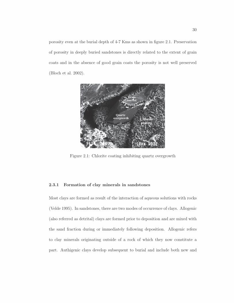
30

porosity even at the burial depth of 4-7 Kms as shown in figure 2.1. Preservation

of porosity in deeply buried sandstones is directly related to the extent of grain

coats and in the absence of good grain coats the porosity is not well preserved

(Bloch et al. 2002).

Figure 2.1: Chlorite coating inhibiting quartz overgrowth

2.3.1 Formation of clay minerals in sandstones

Most clays are formed as result of the interaction of aqueous solutions with rocks

(Velde 1995). In sandstones, there are two modes of occurrence of clays. Allogenic

(also referred as detrital) clays are formed prior to deposition and are mixed with

the sand fraction during or immediately following deposition. Allogenic refers

to clay minerals originating outside of a rock of which they now constitute a

part. Authigenic clays develop subsequent to burial and include both new and

31

regenerated forms. Authigenic clay minerals are formed or regenerated in place.

Authigenic clays form as a direct precipitate from formation waters (neoforma-

tion) or through reactions between precursor materials and the contained waters

(regenerated) (Wilson and Pittman 1977).

Clays generally are degraded during weathering, erosion and transport and

generated or regenerated during burial diagenesis. Authigenic clays can be differ-

entiated from Allogenic (detrital) clays on the basis of clay composition, structure,

morphology and distribution and textural properties. For example, presence of

delicate clay morphology (rosette or vermicular aggregates) hints at authigenic

origin because delicate clay morphologies are very unlikely to be intact during

sedimentary transport (Wilson and Pittman 1977). Authigenic grain coating

clays are usually absent only at grain contacts (Wilson and Pittman 1977).

2.3.2 Morphology of authigenic clays

Authigenic clays can be easily identified based on their morphology. Three

most common morphologies of authigenic clays are pore-fillings, pore-linings (also

called clay films, or grain coating) and replacements. Kaolinite and dickite are

most common pore-filling clays. Kaolinite forms in sediments by the action of

low-pH ground waters on detrital aluminosilicate minerals such as feldspars, mica,

rock fragments and heavy minerals (Velde 1995). Kaolinite almost always occurs

as pseudohexagonal plates in the form of books (stacked plates) or as a deli-

32

cate vermicular growth, a sequence of stacked pseudohexagonal plates that may

extend length of a pore as shown in the figure 2.2 (Wilson and Pittman 1977).

With progressive increase in burial depth and temperature (2-3 km, T=70-900C),

thin booklet-like kaolinite is progressively transformed into thick, well-developed

crystals called dickite (Worden and Morad 2003). Pore-filling clays plug inter-

Figure 2.2: (A) Stacked plates of kaolinite in porous sandstone (face-to-face ar-rangement and pseudohexagonal outlines of individual plates) (B) Vermicularauthigenic kaolinite in porous sandstone (Wilson and Pittman 1977)

stitial pores and individual flakes or aggregates of the flakes exhibit no apparent

alignment relative to the detrital grain surfaces.

Pore linings are formed by clay coatings deposited on the surfaces of frame-

work grains, except at points of grain-to-grain contact. Clay particles usually

exhibit a preferred orientation normal to or parallel to the detrital grain surface.

Illite is a grain coating clay but appears as irregular flakes with fiber or lath-like

33

projections. Occasionally, the sheets of illite may develop relatively long, delicate

appearing, lath-like projections and may measure up to 30 µm long and range

from 0.5 to 2 µm in width as shown in figures 2.3 and 2.4.

Figure 2.3: SEM image of illite, showing lath-like projections which extend fromone grain to another (Storvoll et al. 2002)

Chlorite is an important pore lining clay. Authigenic chlorite occurs primarily

as pore-lining pseudohexagonal flakes with a cardhouse, honeycomb or rosette

arrangement (Hayes 1970). Figures 2.5 and 2.6 show grain coating chlorite clay

at different magnifications. We observe that the crystals appear attached to sand

grains along their longest dimension. Chlorite flakes are generally 2-10 µm across

with a thickness of approximately 0.1 µm. Figure 2.7 show the delicate rosette

like arrangement of chlorite crystals.

34

Figure 2.4: SEM image of illite, showing delicate fiber like structure (Storvollet al. 2002)

Figure 2.5: SEM images of grain coating chlorite at different magnifications. Theimages on left and right are at 50 and 400 magnifications respectively (Cerepiet al. 2002)

35

Figure 2.6: SEM images of grain coating chlorite at different magnifications.The images on left and right are at 1,000 and 10,000 magnifications respectively(Cerepi et al. 2002)

Figure 2.7: Chlorite clay exhibiting delicate rosette like morphology (Wilson andPittman 1977)

36

2.3.3 Effect of grain coating chlorite on formation evaluation

Presence of chlorite clays affect wireline and NMR measurements (Claudine et al.

2001, Rueslatten et al. 1998). Claudine et al. (2001) argued that chlorite bearing

sandstones usually give low resistivity signals and can lead to overestimation of

water saturations while interpreting the logs. Rueslatten et al. (1998) validated

NMR logs from sandstone oil reservoir offshore Mid Norway by taking into ac-

count pore lining iron rich chamosite and concluded that the faster T2 decay is

due to the magnetic field inhomogeneities caused by chlorite clays on pore scale.

Pore-lining chlorite acts as micropores and if the diffusion of spins from macrop-

ore to micropore surface is not fast both micropore and macropore do not relax

independent of each other. Diffusional coupling and internal field gradients be-

come very important consideration when interpreting NMR logs from reservoirs

which contain significant amount of pore lining clay.

Straley et al. (1995) compared FFI derived from borehole NMR logs with

laboratory-measured values of the centrifugeable water for the core samples con-

taining significant amount of pore-lining authigenic chlorite clay. They found

that T1 distribution for partially saturated cores shifts towards shorter T1 com-

ponents. They observed that the peak amplitude of shorter T1 component for

partially saturated cores is larger than that of for fully saturated cores. This

observation can be explained by taking into account increased value of surface

37

to volume ratio (S/V ) for partially saturated cores. When the sample is fully

water saturated, macropores open into microchannel created by pore-lining clay

flakes. For the fast diffusion limit, the whole micropore has a single relaxation

time characterized by surface to volume ratio (S/V ). For partially saturated core

samples, the micropores are still saturated with water while the macropores are

drained. This results in higher value of surface to volume ratio (S/V ) because

even though the relaxing surface area is the same, the volume of water has greatly

decreased.

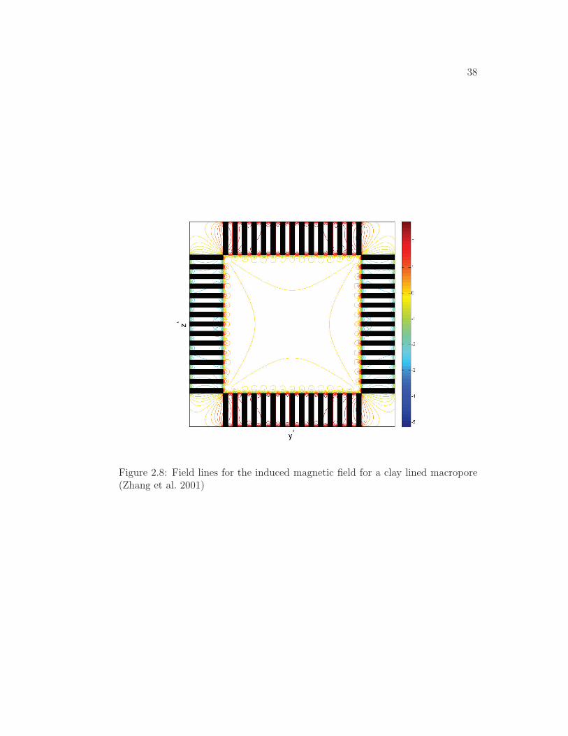
Zhang, Hirasaki and House (2001, 2003) used a simplified model to compute

the magnitude of internal field gradients in a clay coated sandstones and com-

pared with experimental data. They reported that in clay-lined sandstones the

magnitude of internal field gradients can be as high as ∼300 Gauss/cm which can

be much greater than the gradient applied by the logging tool. They also studied

a one dimensional system with constant gradient under restricted diffusion.

Next chapter describes a two dimensional model to explain transverse relax-

ation in a macropore which contains a clay flake.

38

Figure 2.8: Field lines for the induced magnetic field for a clay lined macropore(Zhang et al. 2001)

39

Figure 2.9: Contours of dimensionless magnetic field gradient for a claylinedmacropore (Zhang et al. 2001)

40

Chapter 3

Modeling Internal Field Gradients in clay-lined

sandstones

The apparent similarity of the NMR surface relaxivity of sandstones has led to

the adoption of a default value of T2 irreducible water cut-off for all sandstones.

Carbonate rocks do not exhibit strong echo spacing dependence of transverse

relaxation. However, T2 distribution is strongly dependent on echo spacing for

chlorite clay-lined sandstones and sandstones which contains large amounts of

paramagnetic minerals. Such sandstones should be treated differently and a

generalized theory to understand the effect of internal field gradients on transverse

relaxation is needed.

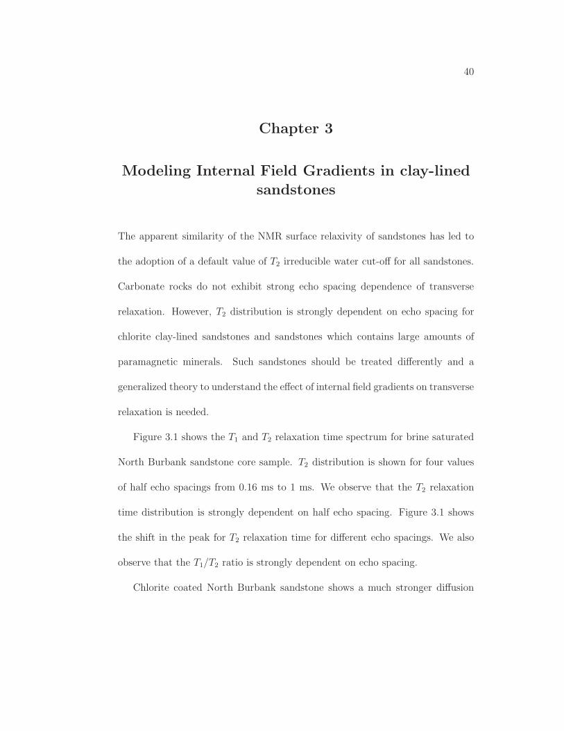
Figure 3.1 shows the T1 and T2 relaxation time spectrum for brine saturated

North Burbank sandstone core sample. T2 distribution is shown for four values

of half echo spacings from 0.16 ms to 1 ms. We observe that the T2 relaxation

time distribution is strongly dependent on half echo spacing. Figure 3.1 shows

the shift in the peak for T2 relaxation time for different echo spacings. We also

observe that the T1/T2 ratio is strongly dependent on echo spacing.

Chlorite coated North Burbank sandstone shows a much stronger diffusion

41

� � � � � � � � � � � � � � � � � � ��

� �� ! "

τ # � � � $ % & ! "τ # � � $ % & ! "τ # � � � � $ % & ! "τ # � � � $ % & '

Figure 3.1: T1 and T2 relaxation time spectrum for North Burbank core samplesaturated with brine solution

effect due to internal field gradients. North Burbank sandstone is chamosite

coated (Trantham and Clampitt 1977). A common feature of the chamosite is

that it is an iron rich chlorite and is pore lining (Zhang, Hirasaki and House 2003).

North Burbank sandstone has a T1/T2 and ρ2/ρ1 ratio that is larger than most

values reported in the literature (Zhang and Hirasaki 2003, Zhang et al. 2003).

Figure 3.2 shows a schematic of a claylined pore. Clay flakes form microchan-

nels in the macropore which are called micropores. Clay flakes have a different

magnetic susceptibility than that of pore filling fluid. In order to model the ef-

fect of internal field gradients on transverse relaxation due to the presence of

42

( ) * + , - . / 0 * 1 2 /3 - 4 , + 4 ) 1 5 5 / *3 1 4 , + 6 + , /

Figure 3.2: Schematic of a macropore lined with clay flakes

43

clay flakes in sandstones, we consider a clay-lined pore as described in figure

3.2. Figure 3.3 and 3.4 show the simplified geometry for simulation purpose.

Only one-fourth of the pore is considered because of the presence of symmetry

boundary planes as marked in figure 3.3 and 3.4. The clay flake is assumed to be

infinitely long in ± x directions. This strikes out any dependence of x co-ordinate

and effectively makes the model two dimensional. η and λ are the aspect ratio

for the macropore and clay flake respectively, and β is the microporosity fraction.

The induced magnetic field due to the presence of clay flake can be calculated

Figure 3.3: Schematic of a clay-lined pore

using Green’s function in two dimensions (Zhang et al. 2003). The following is

44

Figure 3.4: Schematic of the simulation domain

the expression for the induced magnetic field due to a clay flake.

Bδz =B0∆χ

2π

[

tan−1

(

λ (β − z∗)

(y∗λ− β)

)

+ tan−1

(

λ (β + z∗)

(y∗λ− β)

)

− tan −1

(

λ (β − z∗)

(y∗λ+ β)

)

− tan −1

(

λ (β + z∗)

(y∗λ+ β)

)]

(3.1)

Where y∗ = y/L2 and z∗ = z/L2 are dimensionless y and z coordinates.

45

7 89:

; ; < = ; < > ; < ? ; < @ A;; < A; < =; < B; < >; < C; < ?; < D; < @; < EA

(a)

F GHI

J K L J K M J K N J K O J K P J K Q J K R J K S J K TJ K LJ K MJ K NJ K OJ K PJ K QJ K RJ K SJ K T

(b)

Figure 3.5: (a) Field lines of the total magnetic field B due to the clay flake in ahomogeneous field B0 (b) Field lines of the induced magnetic field Bδ due to theclay flake in a homogeneous field B0

U VWX

Y Z [ Y Z \ Y Z ] Y Z ^Y Z _Y Z [Y Z `Y Z \Y Z aY Z ]Y Z bY Z ^Y Z cd `d [d _Y _[

(a)

e e f g e f h e f i e f j e fk e f l e f m e f n e f oee f ge f he f ie f je f ke f le f me f ne f op q

rs t u vw xyz{ | }~� � ��

��

(b)

Figure 3.6: (a) Contour lines of the z component of induced field (b) Contoursof dimensionless gradient due to the presence of clay flake

46

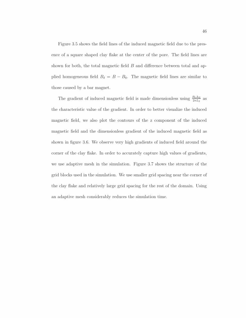
Figure 3.5 shows the field lines of the induced magnetic field due to the pres-

ence of a square shaped clay flake at the center of the pore. The field lines are

shown for both, the total magnetic field B and difference between total and ap-

plied homogeneous field Bδ = B − B0. The magnetic field lines are similar to

those caused by a bar magnet.

The gradient of induced magnetic field is made dimensionless using B0∆χ2πL2

as

the characteristic value of the gradient. In order to better visualize the induced

magnetic field, we also plot the contours of the z component of the induced

magnetic field and the dimensionless gradient of the induced magnetic field as

shown in figure 3.6. We observe very high gradients of induced field around the

corner of the clay flake. In order to accurately capture high values of gradients,

we use adaptive mesh in the simulation. Figure 3.7 shows the structure of the

grid blocks used in the simulation. We use smaller grid spacing near the corner of

the clay flake and relatively large grid spacing for the rest of the domain. Using

an adaptive mesh considerably reduces the simulation time.

47

� � � � � � � � � � � � � ��

� ��

� ��

Figure 3.7: Schematic of mesh used to resolve large values of gradients aroundthe corner

48

3.1 Simulations for FID and CPMG pulse sequence

This section describes the procedure for the simulation of Free Induction Decay

(FID) and Carr-Purcell-Meiboom-Gill (CPMG) pulse sequence for a macropore

which contains a clay flake. The Transverse relaxation is simulated in y-z plane.

We start with Bloch-Torrey equations for the transverse magnetization after the

application of a 900 pulse. The applied magnetic field is in the z direction, B0.

3.1.1 Governing equations

The Governing equations are Bloch-Torrey equations which are described below

(Torrey 1956).

∂Mx

∂t= γMyBz −

Mx

T2B+D∇2Mx (3.2)

∂My

∂t= −γMxBz −

My

T2B

+D∇2My (3.3)

Where, Mx and My are the x and y components of the magnetization, γ is the

gyromagnetic ratio of the proton, T2B is the bulk transverse relaxation time and

Bz is the z component of the magnetic field. If we assume M = Mx + iMy,

then the above equations can be described by a single equation (Bergman and

Dunn 1995a).

∂M

∂t= −iγMBz −

M

T2B

+D∇2M (3.4)

49

When, M = m exp[

−iω0t− tT2B

]

is substituted in equation 3.4, the equation is

transformed into rotating co-ordinate frame and bulk relaxation term is factored

out. The resulting equation is:

∂m

∂t= −iγmBδz +D∇2m (3.5)

Where, Bδz = Bz − B0 and m is a complex variable (m = mR + imI). The

expression for Bδz is given by equation 3.1.

For the sake the convenience, now onwards we shall refer Bδz =B0∆χ2π

F (y∗, z∗)

so that the dependence of y∗ and z∗ is represented by F (y∗, z∗). This yields a

simple equation which is as follows.

∂m

∂t= −−iγB0∆χ

2πF (y∗, z∗)m+D∇2m (3.6)

3.1.2 Boundary and Initial conditions

At symmetry planes zero flux condition for magnetization is applied. At the

relaxation boundary, the Fourier boundary condition is used. At initial time a

50

uniform magnetization through out the pore space is assumed.

n · ∇m = 0 : at symmetry planes

Dn · ∇m + ρ m = 0 : at micropore surface

m(t = 0) = m0 : uniform magnetization throughout the pore

Where, D is the free diffusion coefficient and ρ is the surface relaxivity for trans-

verse relaxation.

3.2 Dimensionless groups and their significance

The governing equations and boundary conditions are made dimensionless with

characteristic scales, x0, t0 and m0. x0 is taken as half length of the macropore,

L2, and m0 as the initial uniform magnetization. The characteristic time scale is

taken as the time for significant dephasing of spins, τω = 1

δω. δω is the spread of

Larmor frequency which is given as:

τω =1

δω=

1

γgL2

(3.7)

Where, g characterizes the internal field gradients. Using the concept of effective

gradients developed by Hurlimann (1998), g and τω can be described by the

51

following expressions.

g = |∇B| ' B0∆χ

L2

(3.8)

τω =1

δω=

1

γB0∆χ(3.9)

Other timescales are diffusional correlation time τR =L22

Dand half echo spacing

τE . The characteristic scales and respective dimensionless variables are described

below.

x0 = L2 : Half length of the macropore

t0 = τω =1

δω=

1

γB0∆χ: Time for significant dephasing

m0 = m0 : Initial magnetization

m∗ =m

m0

y∗ =y

L2

, z∗ =z

L2

t∗ =t

τω

τ ∗E =τEτω

= δωτE

τ ∗R =τRτω

= δωτR

52

Using dimensionless variables, the governing equations become:

(

L22

D

)

(

1

γB0∆χ

)

∂m∗

∂t∗=

−i

2π

(

L22

D

)

(

1

γB0∆χ

)F (y∗, z∗)m∗ +∇∗2m∗ (3.10)

Equation 3.10 can be further simplified by identifying the dimensionless groups.

ζ∂m∗

∂t∗=

−i

2πζF (y∗, z∗)m∗ +∇∗2m∗ (3.11)

Equation 3.10 contains the dimensionless group ζ which is defined below.

ζ =τRτω

=

(

L22

D

)

(

1

γB0∆χ

) =γB0∆χL2

2

D(3.12)

ζ is the ratio of two timescales present in the system. First is the diffusional

correlation time (τR =L22

D) and another is the time for significant dephasing (τω =

1

γB0∆χ). For simulating CPMG pulse sequence, the third characteristic timescale

is the dimensionless echo spacing, τ ∗E=τE/τω.

The other dimensionless parameters are geometrical parameters namely as-

pect ratio of the macropore (η), aspect ratio of the clay flake (λ) and the micro-

porosity fraction (β).

Equation 3.11 with given boundary and initial conditions is solved using finite

difference method in residual form. Iterative Alternating Direction Implicit (ADI)

method (Peaceman and Rachford Jr 1955) is used for integrating the difference

53

equations in time. The macroscopic magnetization is calculated by taking the

magnitude of the sum of individual magnetization vectors over all the grid blocks.

The dependence of timestep size was examined and the optimum value of the

timestep size was used for all simulations.

In the following simulation results, the surface relaxivity (ρ) is taken as zero

which means the decay of NMR signal is caused solely by the diffusion of spins

under the influence of inhomogeneous magnetic field. The subsequent sections

discuss the secular relaxation for free induction decay (FID) and CPMG pulse

sequence.

3.3 FID results and discussion

Free induction decay (FID) can be easily simulated by starting with initial uni-

form magnetization. As spins diffuse under the influence of internal field gra-

dients, they precess with different Larmor frequency and this causes the loss of

phase coherence leading to the decay of the magnetization.

Figure 3.8 show the decay of magnetization for different values of ζ=τR/τω.

For small values of ζ , we see a single-exponential decay of magnetization. How-

ever, when the values of ζ is more than 20, free induction decay (FID) is not

monotonically decreasing. The magnetization drops by two orders of magnitude

and begins to rise again. These undulations finally die out in the noise level. It is

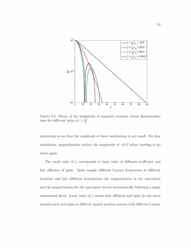
54

� � � � � � � � � � � � � � ¡ � ¢ �� £ ¤� � £ ¥� � ¦

§ ¨©ª

ζ « τ¬ τω

« ® ¯ ° ¯ζ « τ¬ τ

ω« ± ¯ ° ¯

ζ « τ¬ τω

« ² ¯ ° ¯ζ « τ¬ τ

ω« ® ¯ ¯ ° ¯

Figure 3.8: Decay of the magnitude of magnetic moment versus dimensionlesstime for different value of ζ= τR

τω

interesting to see that the amplitude of these undulations is not small. For first

undulation, magnetization reaches the magnitude of ∼0.2 before starting to go

down again.

The small value of ζ corresponds to large value of diffusion coefficient and

fast diffusion of spins. Spins sample different Larmor frequencies at different

locations and fast diffusion homogenizes the magnetization in the macropore

and the magnetization for the macropore decays monotonically following a single

exponential decay. Large value of ζ means slow diffusion and spins do not move

around much and spins at different spatial position precess with different Larmor

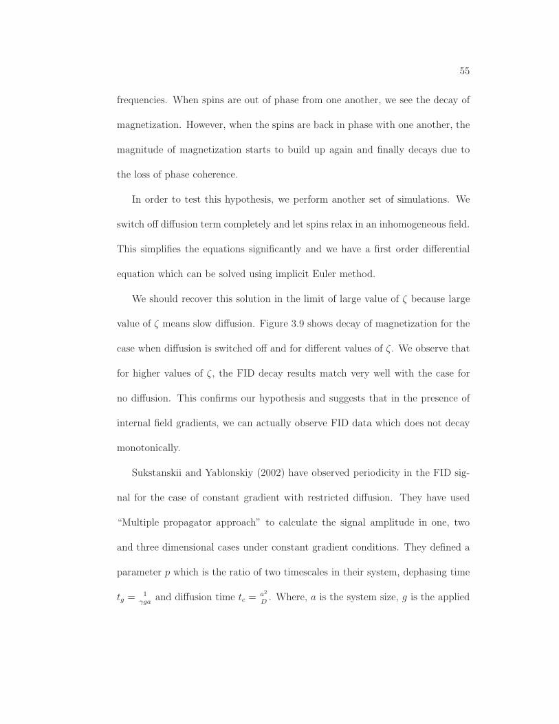
55

frequencies. When spins are out of phase from one another, we see the decay of

magnetization. However, when the spins are back in phase with one another, the

magnitude of magnetization starts to build up again and finally decays due to

the loss of phase coherence.

In order to test this hypothesis, we perform another set of simulations. We

switch off diffusion term completely and let spins relax in an inhomogeneous field.

This simplifies the equations significantly and we have a first order differential

equation which can be solved using implicit Euler method.

We should recover this solution in the limit of large value of ζ because large

value of ζ means slow diffusion. Figure 3.9 shows decay of magnetization for the

case when diffusion is switched off and for different values of ζ . We observe that

for higher values of ζ , the FID decay results match very well with the case for

no diffusion. This confirms our hypothesis and suggests that in the presence of

internal field gradients, we can actually observe FID data which does not decay

monotonically.

Sukstanskii and Yablonskiy (2002) have observed periodicity in the FID sig-

nal for the case of constant gradient with restricted diffusion. They have used

“Multiple propagator approach” to calculate the signal amplitude in one, two

and three dimensional cases under constant gradient conditions. They defined a

parameter p which is the ratio of two timescales in their system, dephasing time

tg =1

γgaand diffusion time tc =

a2

D. Where, a is the system size, g is the applied

56

� � � � � � � � � � � �� £ ¤� � £ ¥� � ¦

§ ¨©ª

³ ´ µ ¶ · · ¸ ¹ ¶ ´ º »ζ ¼ τ½ ¾ τ

ω→ ∞¿ À µ »

ζ ¼ τ½ ¾ τω

¼ Á Â Â¿ À µ »ζ ¼ τ½ ¾ τ

ω¼ Ã Â Â¿ À µ »

ζ ¼ τ½ ¾ τω

¼ Á Â Â Â¿ À µ »ζ ¼ τ½ ¾ τ

ω¼ Á Ã Â Â

Figure 3.9: Comparison of FID decay of magnetization for different values of ζ= τR

τωand for the case when no diffusion is present

gradient and D is the self-diffusion coefficient. Periodic FID signal is observed

when the value of parameter p is less then 0.3.

3.4 CPMG results and discussion

The program for FID decay can be easily modified for CPMG pulse sequence.

For CPMG pulse sequence, at t = τE , 3τE , 5τE and so on, we apply a 1800

pulse which is equivalent to m(t = τ+E ) = m(t = τ−E ), where m represents the

transpose of the m. This effectively means that 1800 pulse reverses the direction

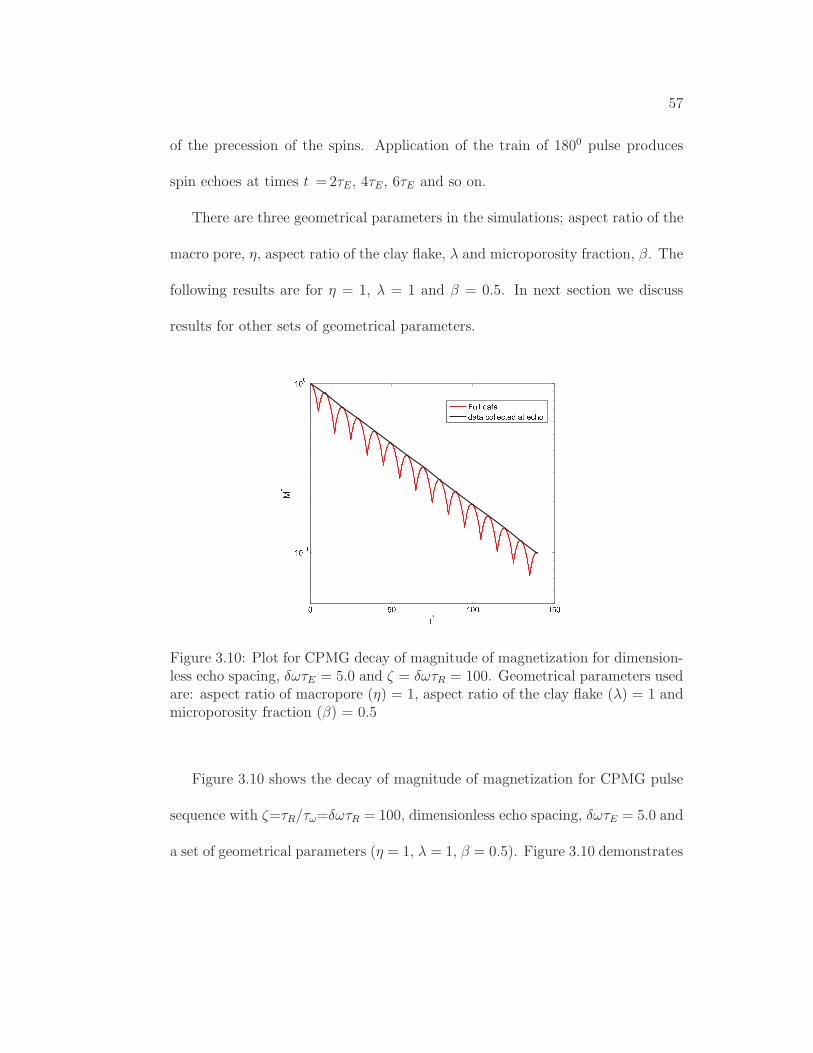
57

of the precession of the spins. Application of the train of 1800 pulse produces

spin echoes at times t =2τE, 4τE, 6τE and so on.

There are three geometrical parameters in the simulations; aspect ratio of the

macro pore, η, aspect ratio of the clay flake, λ and microporosity fraction, β. The

following results are for η = 1, λ = 1 and β = 0.5. In next section we discuss

results for other sets of geometrical parameters.

Ä Å Ä Æ Ä Ä Æ Å ÄÆ Ä Ç ÈÆ Ä É

ÊËÌ Í

Î Ï Ð Ð Ñ Ò Ó ÒÑ Ò Ó Ò Ô Õ Ð Ð Ö Ô Ó Ö Ñ Ò Ó Ö Ô × Õ

Figure 3.10: Plot for CPMG decay of magnitude of magnetization for dimension-less echo spacing, δωτE = 5.0 and ζ = δωτR = 100. Geometrical parameters usedare: aspect ratio of macropore (η) = 1, aspect ratio of the clay flake (λ) = 1 andmicroporosity fraction (β) = 0.5

Figure 3.10 shows the decay of magnitude of magnetization for CPMG pulse

sequence with ζ=τR/τω=δωτR = 100, dimensionless echo spacing, δωτE = 5.0 and

a set of geometrical parameters (η = 1, λ = 1, β = 0.5). Figure 3.10 demonstrates

58

that a train of 1800 pulses refocus the magnetization and secular relaxation follows

a single exponential decay.

For a given set of geometrical parameters, we summarize our results in terms

of two parameters. First is ζ = δωτR, which is the ratio of τR and τω and second

is dimensionless half-echo spacing, τ ∗E = δωτE which is the ratio of τE and τω.

We fit a single-exponential curve for the decay of magnetic moment and calculate

dimensionless secular relaxation rate for each parameter value.

The magnetization decay is bi-exponential for the simulations where ζ=τR/τω

is more than 1000. A few of these cases are illustrated in figures 3.11, 3.12 and

3.13. For such cases, slower component of bi-exponential decay is taken as the

relaxation rate. Using these values of the dimensionless transverse relaxation

rate, we create a single plot which shows the relaxation rates for all parameter

values which is illustrated in figure 3.15.

Based on the relative magnitudes of three timescales, three different charac-

teristic relaxation regimes are defined (Anand and Hirasaki 2007b).

Motionally averaging regime: This regime is characterized by fast diffu-

sion of protons such that the inhomogeneities in the magnetic field are motionally

averaged. This occurs when the diffusional correlation time (τR) is the smallest

timescale and is much shorter compared to half echo spacing and the time taken

for significant dephasing due to presence of field inhomogeneities. In this regime,

the secular relaxation rate does not show any dependence on echo spacing. The

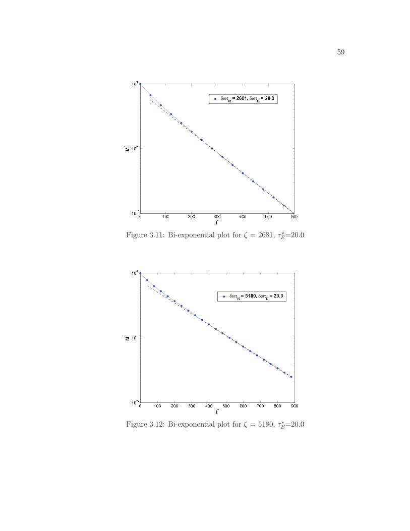
59

Ø Ù Ø Ø Ú Ø Ø Û Ø Ø Ü Ø Ø Ý Ø Ø Þ Ø ØÙ Ø ß àÙ Ø ß áÙ Ø â

ã äåæ

δωτç è é ê ë ì í δωτî è é ï ð ï

Figure 3.11: Bi-exponential plot for ζ = 2681, τ ∗E=20.0

Ø Ù Ø Ø Ú Ø Ø Û Ø Ø Ü Ø Ø Ý Ø Ø Þ Ø Ø ñ Ø Ø ò Ø Ø ó Ø ØÙ Ø ß àÙ Ø ß áÙ Ø â

ã äåæ δωτç è ô ì ë ï í δωτî è é ï ð ï


60

Ø Ù Ø Ø Ú Ø Ø Û Ø Ø Ü Ø Ø Ý Ø Ø Þ Ø Ø ñ Ø Ø ò Ø Ø ó Ø ØÙ Ø ß á

Ù Ø â

ã äåæ δωτç è ì ï ï ï ï í δωτî è é ï ð ï


conditions for motionally averaging regime are:

τR << τω (3.13)

τR << τE

Free diffusion regime: This regime is valid when half echo spacing is the

shortest timescale. The effect of restriction as well as large field inhomogeneities

are not felt by the spins in the time of echo formation. Thus, spins dephase as if

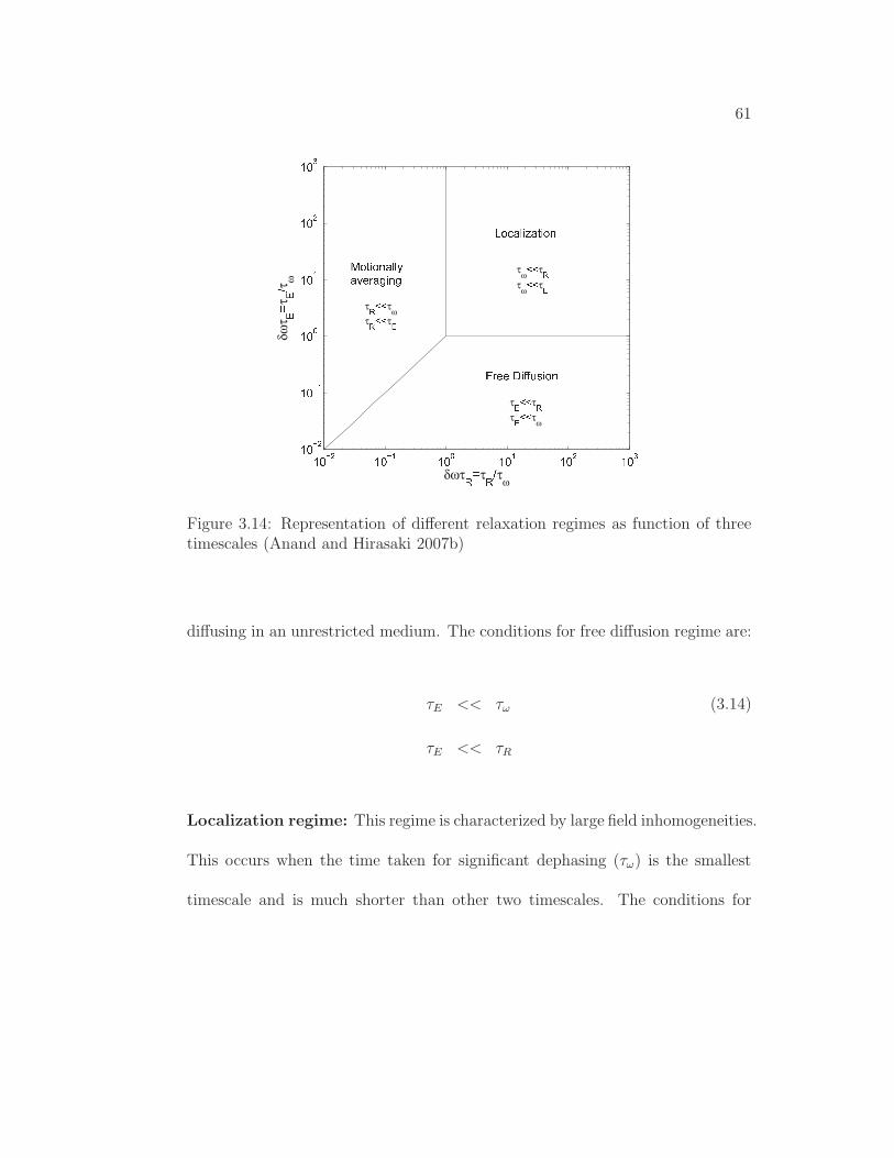
61

õ ö ÷ ø õ ö ÷ ù õ ö ú õ ö ù õ ö ø õ ö ûõ ö ÷ øõ ö ÷ ùõ ö úõ ö ùõ ö øõ ö û

δωτ ü ý τ ü þ τω

δωτ

ÿ� τÿ� τ ω

� � � � � � � � � � � � � � � � � � � � � � � � � � ��

τω

� �τ �

τω

� �τ �

τ � � �τ �

τ � � �τ

ω

τ � � �τ

ωτ � � �

τ �Figure 3.14: Representation of different relaxation regimes as function of threetimescales (Anand and Hirasaki 2007b)

diffusing in an unrestricted medium. The conditions for free diffusion regime are:

τE << τω (3.14)

τE << τR

Localization regime: This regime is characterized by large field inhomogeneities.

This occurs when the time taken for significant dephasing (τω) is the smallest

timescale and is much shorter than other two timescales. The conditions for

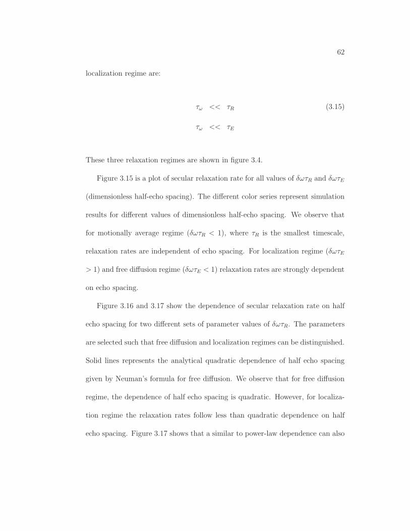
62

localization regime are:

τω << τR (3.15)

τω << τE

These three relaxation regimes are shown in figure 3.4.

Figure 3.15 is a plot of secular relaxation rate for all values of δωτR and δωτE

(dimensionless half-echo spacing). The different color series represent simulation

results for different values of dimensionless half-echo spacing. We observe that

for motionally average regime (δωτR < 1), where τR is the smallest timescale,

relaxation rates are independent of echo spacing. For localization regime (δωτE

> 1) and free diffusion regime (δωτE < 1) relaxation rates are strongly dependent

on echo spacing.

Figure 3.16 and 3.17 show the dependence of secular relaxation rate on half

echo spacing for two different sets of parameter values of δωτR. The parameters

are selected such that free diffusion and localization regimes can be distinguished.

Solid lines represents the analytical quadratic dependence of half echo spacing

given by Neuman’s formula for free diffusion. We observe that for free diffusion

regime, the dependence of half echo spacing is quadratic. However, for localiza-

tion regime the relaxation rates follow less than quadratic dependence on half

echo spacing. Figure 3.17 shows that a similar to power-law dependence can also

63

be observed if during crossover from one regime to another.

In order to better visualize all three regimes on the same plot, we plot the

contours of the secular relaxation rate. Figure 3.18 shows the plot of simulated

dimensionless relaxation rates (1/T ∗

2, secular) as a function of δωτR for different

values of δωτE. We observe that for motionally averaging regime, the contour

lines are vertical and show no dependence on echo spacing. For free diffusion and

localization regimes, contour lines are dependent on echo spacing.

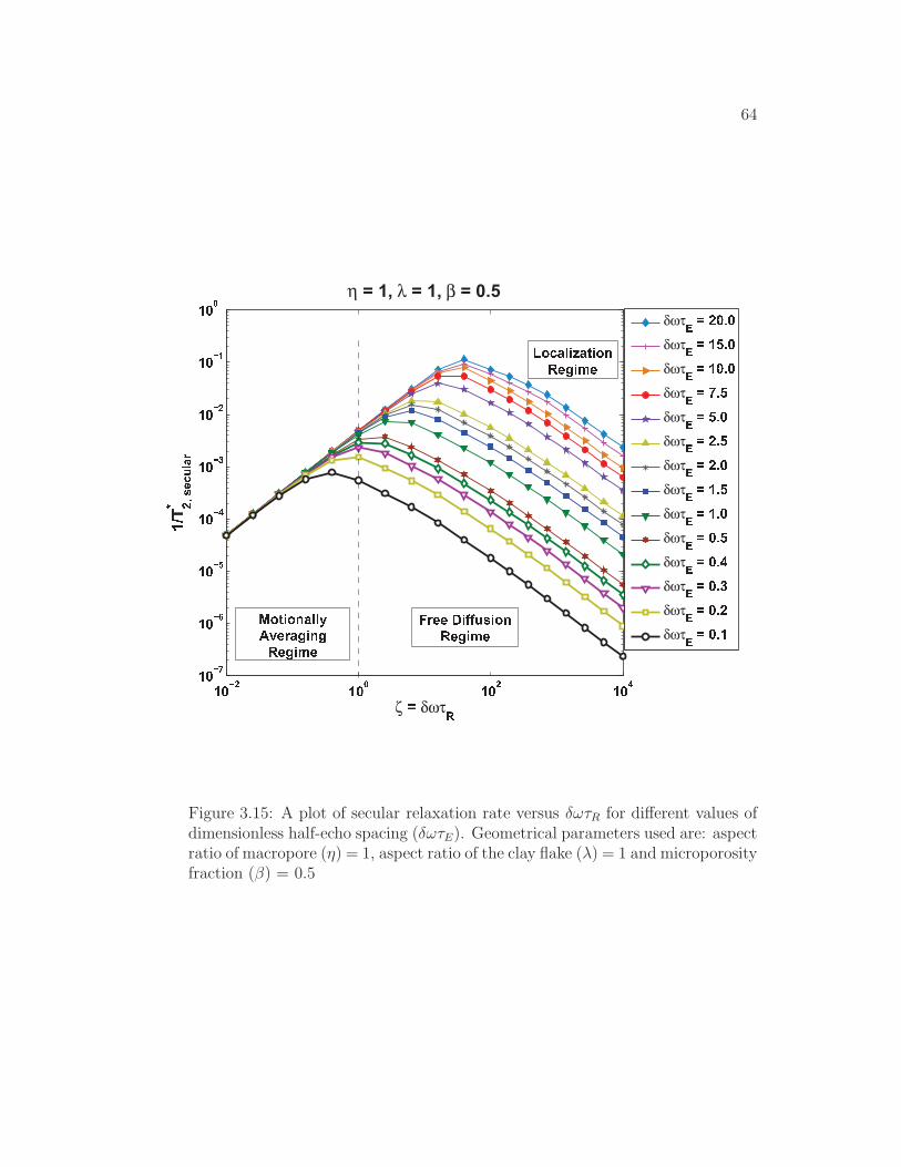
64

� � � � � � � � � � � � �� !� � � �� "� � � �� #� � �

ζ $ δωτ%&'( ) *+,-./ 012

η λ β

δωτ 3 4 5 � 6 �δωτ 3 4 � 7 6 �δωτ 3 4 � � 6 �δωτ 3 4 8 6 7δωτ 3 4 7 6 �δωτ 3 4 5 6 7δωτ 3 4 5 6 �δωτ 3 4 � 6 7δωτ 3 4 � 6 �δωτ 3 4 � 6 7δωτ 3 4 � 6 9δωτ 3 4 � 6 :δωτ 3 4 � 6 5δωτ 3 4 � 6 �; < = = > ? @ @ A B ? C DE = F ? G =H C I ? C D J K K LM N = < J F ? D FE = F ? G =

O C P J K ? Q J I ? C DE = F ? G =

Figure 3.15: A plot of secular relaxation rate versus δωτR for different values ofdimensionless half-echo spacing (δωτE). Geometrical parameters used are: aspectratio of macropore (η) = 1, aspect ratio of the clay flake (λ) = 1 and microporosityfraction (β) = 0.5

65

R S T U R S V R S UR S T WR S T XR S T YR S T ZR S T [R S T \R S T U

δωτ]_ a bc defg hij

η k l m λ k l m β k n o pδωτq r s t t t tδωτq r u s v tδωτq r s w x t

y z { | } ~ � | � ~ z � � � � ~ � �� ~ � � � � ~ z � � � � ~ � �

Figure 3.16: Plot of secular relaxation rate as function of δωτE for different valuesof δωτR. Geometrical parameters used are: aspect ratio of macropore (η) = 1,aspect ratio of the clay flake (λ) = 1 and microporosity fraction (β) = 0.5

66

Figure 3.17: Plot of secular relaxation rate as function of δωτE for different valuesof δωτR demonstrating various echo-spacing dependence in different regimes

67

ζ � τ � � τω

� δωτ �

δωτ

�ì ï � � ì ï � � ì ï � ì ï � ì ï � ì ï � ì ï �ì ï � �

ì ï �ì ï � � � � � �� ¡ ¢ £ ¤ ¡ ¥ £ � ¦§ ¨ © £ ª ¨

« ¬ ¨ ¨ £ ® ® ¯ ° £ � ¦§ ¨ © £ ª ¨± � ¥ £ � ¦ ¡ ¢ ¢ ² ³ ´ ¨ ¬ ¡ © £ ¦ ©§ ¨ © £ ª ¨

Figure 3.18: Contours of secular relaxation rate as a function of δωτR for differentvalues of δωτE . Geometrical parameters used are: aspect ratio of macropore (η)= 1, aspect ratio of the clay flake (λ) = 1 and microporosity fraction (β) = 0.5

68

3.5 Simulations for other geometrical parameters

µ ¶ · ¸ µ ¶ · ¹ µ ¶ º µ ¶ ¹ µ ¶ ¸ µ ¶ » µ ¶ ¼µ ¶ · ½µ ¶ · ¾µ ¶ · ¼µ ¶ · »µ ¶ · ¸µ ¶ · ¹

ζ ¿ δωτ ÀÁÂÃ Ä ÅÆÇÈÉÊ ËÌÍ

η Î Ï Ð Ñ λ Î Ï Ð Ñ β Î Ð Ò ÓδωτÔ Õ Ö ¶ × ¶δωτÔ Õ µ Ø × ¶δωτÔ Õ µ ¶ × ¶δωτÔ Õ Ù × ØδωτÔ Õ Ø × ¶δωτÔ Õ Ö × ØδωτÔ Õ Ö × ¶δωτÔ Õ µ × ØδωτÔ Õ µ × ¶δωτÔ Õ ¶ × ØδωτÔ Õ ¶ × ÚδωτÔ Õ ¶ × ÛδωτÔ Õ ¶ × ÖδωτÔ Õ ¶ × µ

Figure 3.19: A plot of secular relaxation rate versus δωτR for different valuesof dimensionless half-echo spacing (δωτE). Geometrical parameters used are:aspect ratio of macropore (η) = 10, aspect ratio of the clay flake (λ) = 10 andmicroporosity fraction (β) = 0.5

The results described in the previous section are valid only for one set of

geometrical parameters and calculated relaxation rates cannot be used for other

values of geometrical parameters. A value of 10 − 100 is more representative of

69

the aspect ratio of macropore. Similarly, photo micrographs of clay flakes reveal

that aspect ratio of the pore lining clay flakes are in the range of 10− 20 (Zhang

and Hirasaki 2003).

Figures 3.19, 3.20, 3.21 and 3.22 describe secular relaxation rate for various

values of geometrical parameters (η, λ and β). The following observations can

be drawn from figures 3.15, 3.19, 3.20, 3.21 and 3.22.

1. We notice that the secular relaxation rate decreases as area fraction of the

clay flake, β2ηλ

decreases from 0.25 (η = 1, λ = 1 and β = 0.5) to 0.05

(η = 100, λ = 20 and β = 0.1).

2. The motionally averaging regime is well defined in all of the cases. For δωτR

< 1, we observe no dependence on echo spacing for a wide range of echo

spacing.

3. The transition from motionally averaging regime to free diffusion or local-

ization regime happens over a large range of parameter δωτR for large values

of η.

The above observations show common features in the results for a wide range

of geometrical parameters. This calls for the need to finding appropriate scaling

parameters to obtain a single master plot for all values of geometrical parameters.

The research work to find scaling parameters is currently under progress.

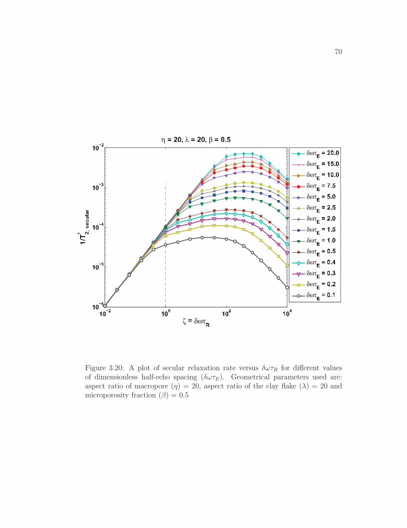
70

� � � � � � � � � � � � �� !� � � �� "� � � �

ζ $ δωτ%&'( ) *+,-./ 012

η $ Ü Ý Þ λ $ Ü Ý Þ β $ Ý ß àδωτ 3 4 5 � 6 �δωτ 3 4 � 7 6 �δωτ 3 4 � � 6 �δωτ 3 4 8 6 7δωτ 3 4 7 6 �δωτ 3 4 5 6 7δωτ 3 4 5 6 �δωτ 3 4 � 6 7δωτ 3 4 � 6 �δωτ 3 4 � 6 7δωτ 3 4 � 6 9δωτ 3 4 � 6 :δωτ 3 4 � 6 5δωτ 3 4 � 6 �


71

� � � � � � � � � � � � �� !� � � �� "� � � �

ζ $ δωτ%&'( ) *+,-./ 012

η λ β

δωτ 3 4 5 � 6 �δωτ 3 4 � 7 6 �δωτ 3 4 � � 6 �δωτ 3 4 8 6 7δωτ 3 4 7 6 �δωτ 3 4 5 6 7δωτ 3 4 5 6 �δωτ 3 4 � 6 7δωτ 3 4 � 6 �δωτ 3 4 � 6 7δωτ 3 4 � 6 9δωτ 3 4 � 6 :δωτ 3 4 � 6 5δωτ 3 4 � 6 �


72

� � � � � � � � � � � � �� á� � � �� !� � � �� "

ζ $ δωτ%&'( ) *+,-./ 012

η λ β

δωτ 3 4 5 � 6 �δωτ 3 4 � 7 6 �δωτ 3 4 � � 6 �δωτ 3 4 8 6 7δωτ 3 4 7 6 �δωτ 3 4 5 6 7δωτ 3 4 5 6 �δωτ 3 4 � 6 7δωτ 3 4 � 6 �δωτ 3 4 � 6 7δωτ 3 4 � 6 9δωτ 3 4 � 6 :δωτ 3 4 � 6 5δωτ 3 4 � 6 �


73

3.6 Conclusions

In this chapter we described a two dimensional model to study transverse relax-

ation in the presence of internal field gradients. Free induction decay (FID) in

the presence of internal field gradients can exhibit non-monotonically decreasing

behavior. This behavior was explained with the help of a test case involving no

diffusion.

A simple two dimensional model is able to capture the spectrum of relaxation

regimes for transverse relaxation. No echo spacing dependence of transverse re-

laxation rate is observed in motionally averaging regime. Localization and free

diffusion regimes show strong dependence of transverse relaxation on echo spac-

ing. Relaxation rates follow quadratic echo spacing dependence in free diffusion

regime while less than quadratic dependence on echo spacing is observed for local-

ization regime. A power-law dependence on echo-spacing is observed for crossover

from one regime to another.

74

Chapter 4

Characterization of pore structure in vuggy

carbonates

More than 50 % of the world’s hydrocarbons are contained in carbonate reservoirs

(Palaz and Marfurt 1997). Accurate characterization of pore structure of carbon-

ate reservoirs is essential for design and implementation of enhanced oil recovery

processes. However, characterizing pore structure in carbonates is a complex task

due to the diverse variety of pore types seen in carbonates and extreme pore level

heterogeneity.

Carbonate reservoirs have complex structures because of depositional and di-

agenetic features. Carbonates may contain not only matrix and fractures but

also vugs. A vug can be defined as any pore that is significantly larger than a

grain or inside of a grain. Vugs are commonly present as leached grains, fos-

sil chambers, fractures, and large irregular cavities. Vugs are irregular in shape

and vary in size from millimeters to centimeters. Vuggy pore space can be di-

vided into separate-vugs and touching-vugs, depending on vug interconnection.

Separate vugs are connected only through interparticle pore networks and do

not contribute to permeability. Touching vugs are independent of rock-fabric

75

Figure 4.1: Core ID-1; Length = 9.0 inches, Diameter = 3.5 inches; Fractured,low porosity, No apparent vugs, uniform cylindrical shape

and form an interconnected pore system enhancing the permeability (Palaz and

Marfurt 1997). Hence, the fluid flow properties like relative permeability depend

on local vug-matrix heterogeneity and connectivity of vugs.

The carbonate samples which are focus of this study are very heterogeneous

in pore structures. Some of the sample rocks are breccia and other samples are

fractured. Some of the typical core samples are shown in the figures 4.1- 4.5. Core

samples of length about 4-9 inches will be used for Tracer experiments. Smaller

plugs of diameter 1.5 inch and length 1.5 inch were drilled from the core samples

which were not well cored (non-uniform cross section) and were unsuitable for

Tracer experiments.

In order to characterize the pore size in vuggy carbonates samples of interest,

we use NMR along with tracer analysis. The distribution of porosity between

micro and macro-porosity can be measured by NMR. However, NMR can not

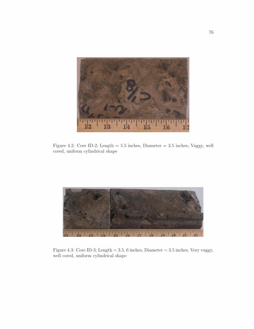
76

Figure 4.2: Core ID-2; Length = 5.5 inches, Diameter = 3.5 inches; Vuggy, wellcored, uniform cylindrical shape

Figure 4.3: Core ID-3; Length = 3.5, 6 inches, Diameter = 3.5 inches; Very vuggy,well cored, uniform cylindrical shape

77

Figure 4.4: Core ID-4; Length = 4 inches, Diameter = 4.0 inches; Some big vugs,well cored

Figure 4.5: Core ID-5; Length = 4.0 inches, Diameter = 4.0 inches; Breccia, veryvuggy and heterogeneous

78

predict if different sized vugs are connected or isolated. Tracer analysis will

be used to characterize the connectivity of the vug system and matrix. Tracer

analysis will also give valuable insight on fraction of dead-end pores and dispersion

effects.

4.1 NMR Experiments

Core-plugs of diameter 1.0 and 1.5 inches and lengths between 1.5 and 3.0 inches

were drilled from the rock samples. The experimental protocol used is as follows:

1. Cleaning: Drilling mud and other solid particles from vugs were removed

using a Water Pik. Core-plugs were first cleaned using a bath of Tetrahy-

drofuran (THF) followed by Chloroform and Methanol. Core-plugs were

dried overnight in the oven at 80 ◦C. Figures 4.6 and 4.7 show the pictures

of core-plugs before and after cleaning. Core-plugs were wrapped in heat

shrink tubing to protect against wear and tear and chipping away of the

sharp edges.

2. After cleaning, core-plugs were saturated with 1 % NaCl brine solution

using vacuum saturation followed by pressure saturation at 1000 psi for 24

hours.

3. Core-plugs were weighed to calculate amount of brine taken during vacuum

and pressure saturation steps.

79

4. Before performing experiment, core-plug was wrapped in paraffin film to

avoid the gravity drainage of brine solution from big vugs.

5. Core-plugs were weighed after experiment to account for any evaporation

of water during the experiment.

Figures 4.6 and 4.7 show the comparison between core-plugs before and after

cleaning. We observe that after cleaning any residual oil is effectively removed

from the core samples and vugs are free of any drilling solids.

4.2 NMR T2 Relaxation and pore size distribution

In this section we describe the T2 relaxation times obtained from NMR measure-

ments on three different core-plugs. NMR experiments were performed on 100 %

brine saturated core-plugs on 2 MHz Maran-SS. For experiments, half-echo spac-

ing of 200 µs was used and signal to noise ratio of 100 was used. Waiting time

of 5 times the largest T2 relaxation time component was used between successive

scans.

Since the carbonate samples do not contain any paramagnetic clays, the shape

of T2 relaxation spectrum is representative of the pore size distribution of the

sample. The largest T2 relaxation component is typically around 2.7 seconds

which corresponds to the T2 relaxation time of the bulk water residing in large

vugs. Smaller relaxation time components represent small sized pores.

80

Figure 4.6: A comparison of before (shown at left) and after (shown at right)cleaned pictures for a core-plug (Plug ID: 3V)

S. No. Core ID Diameter (cm) Length (cm) porosity (%) Type1 3V 3.7 3.2 11.9 vuggy2 2V 3.7 3.6 14.3 vuggy3 1H 3.8 5.7 13.5 vuggy4 5H 3.8 3.3 4.8 no vugs

Table 4.1: Comparison of porosity for different core-plugs

81

Figure 4.7: A comparison of before (shown at left) and after (shown at right)cleaned pictures for a core-plug (Plug ID: 2V)

82

Figures 4.8-4.12 show T2 relaxation time spectrum for various core plugs taken

from different source rocks. Black solid vertical line corresponds to the traditional

cutoff value of 90 ms for carbonate rocks. The dashed vertical line separates the

relaxation spectrum into non-vuggy and vuggy porosity by assuming that T2

values of 750 ms and higher correspond to vugs ((Chang, Vinegar, Morriss and

Straley 1997)). The permeability values for the majority of the core plugs are

within the range of 0.5-6 mD. Figure 4.8 shows the T2 relaxation time spectrum

for a sample which had many visible large solution vugs on the surface. Figure

4.8 shows that for core plug 3V majority of the porosity resides in these large

vugs and contribution of small pore sizes to porosity is very small. NMR response

for core plug 2V (Figure 4.9) shows the peak at relaxation time of about 90 ms.

Using the traditional cut off formula would classify 2V sample as non-pay. The

low value of permeability suggests that the vugs do not form an interconnected

pore network.

Figure 4.10 shows the T2 relaxation time spectrum for a core plug 2VA. Al-

though, this plug was drilled from the same source rock as the previous sample

(Figure 4.9), NMR response shows a large contribution from vugs and relatively

smaller contribution from small sized pores. Figure 4.11 and 4.12 show the T2

relaxation time spectrum for core plugs 1H and 1HA. In both cases, we observe

that relaxation time has contributions from small sized micro-pores, vugs and

some intermediate size pores. The low value of permeability suggests that vugs

83

Figure 4.8: T2 relaxation time spectrum for 100 % brine saturated core-plug (PlugID: 3V)

are isolated vugs and do not create any interconnected flow channels.

NMR results suggest that these carbonate rocks are very heterogeneous. In

some cases, vugs contribute most to the porosity while in other smaller pores are

dominant. Samples taken within the proximity of 3 inches exhibit very different

T2 relaxation time spectrum. Figure 4.13 shows the lack of correlation between

T2 Log mean and the permeability for various core plugs. Chang et al. (1997)

suggested a 750 msec cut off value to calculate the effective T2 Log mean to

correlate with the permeability value. Despite using the 750 msec cut off value to

exclude the vug contribution to permeability, Figure 4.14 shows the lack of any

significant correlation between permeability and T2 Log mean.

84

Figure 4.9: T2 relaxation time spectrum for 100 % brine saturated core-plug (PlugID: 2V)

Figure 4.10: T2 relaxation time spectrum for 100 % brine saturated core-plug(Plug ID: 2VA)

85

Figure 4.11: T2 relaxation time spectrum for 100 % brine saturated core-plug(Plug ID: 1H)

Figure 4.12: T2 relaxation time spectrum for 100 % brine saturated core-plug(Plug ID: 1HA)

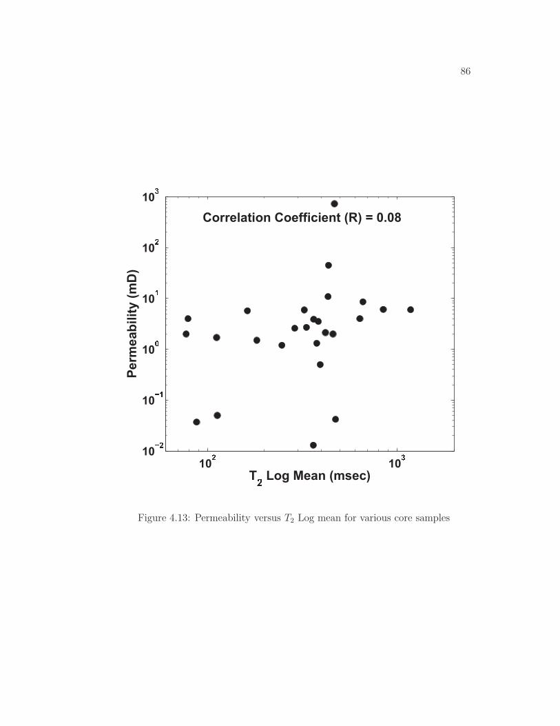
86

â ãä âä åæ åâã

çFigure 4.13: Permeability versus T2 Log mean for various core samples

87

è é êè é ë êè é ë ìè é íè é ìè é êè é î

çFigure 4.14: Permeability versus T2 Log mean while using T2 cut off of 750 msecfor various core samples

88

4.3 Calculating specific surface area of the rock from NMR

T2 distribution

The NMR T2 distribution can be converted into pore size distribution using the

surface relaxivity. The surface relaxivity can be computed by measuring the

NMR T2 relaxation time of 100% brine saturated crushed rock sample in powder

form and the BET surface area of the crushed rock sample. The BET surface

area of the sample was measured to be 1.5 m2/gm.

1

ρT2

=S

VPV=

(

S

W

)

BET

(

φ

1− φ

)

ρg (4.1)

S

VPV=

1

ρ∑

i fi

(

∑

i

fiT2i

)

(4.2)

The above equations can be used to calculate the surface relaxivity using the

NMR T2 distribution and the BET surface area. The value of surface relaxivity

then can be used to calculate the specific surface area of the given sample using

the following relationship:

S

W=

∑

ifiT2i

ρ∑

i fi

(

1− φ

φ

)

1

ρg(4.3)

Where, φ is the porosity,(

SW

)

BETis the BET specific surface area, VPV is the

pore volume of the rock sample, ρg is the grain density and fi is the amplitude

89

of the T2i component in NMR T2 distribution. Figure 4.15 show the relationship

between NMR T2 distribution and the S/V distribution. The S/V distribution

appears as mirror image of the NMR T2 distribution. The figure 4.16 shows the

NMR T2 distribution of the 100% brine saturated crushed rock sample. The

surface relaxivity of the crushed rock sample in powder form was calculated to

be 7.4 µm/sec. This value of surface relaxivity is used to compute the specific

surface area of various rock samples using NMR T2 distribution. Figure 4.17

shows the specific area (m2/gm) of the some of the rock samples. We notice that

the reservoir rock samples have as high as five times the specific surface area of

the Silurian outcrop sample. This difference in specific surface area can result in

higher value of surfactant adsorption for reservoir rock than that for the Silurian

outcrop sample.

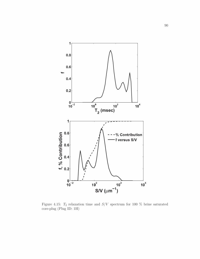
90

ï ð ñ ò ï ð ó ï ð ò ï ð ôðð õ öð õ ÷ð õ øð õ ù ï

ö

ú û ü ý ú û þ ú û ý ú û ÿûû � �û � �û � �û � �ú

µ� ú

� � � � � � � � � � � � � � � � � �

Figure 4.15: T2 relaxation time and S/V spectrum for 100 % brine saturatedcore-plug (Plug ID: 1H)

91

� � � � � � � � � � � � � � � � � � �� !� � "�# $ % & ' ( ) * + , - , . / 0 1 2 ' 34 � 5 6 7 8 9 8 : ; < = 4 ; > 6 ? > @ 6 A B

CDEFFigure 4.16: T2 relaxation time spectrum for 100 % brine saturated crushed rockpowder

Figure 4.17: A bar chart for the specific surface area of several core plugs

92

Figure 4.18: Schematic of the pore system containing interconnect flow channels,touching/isolated vugs and stagnant/dead end pores

4.4 Tracer Analysis

In this section, we describe methods to characterize the key features of pore struc-

ture such as fraction of dead-end pores and dispersion and capacitance effects.

Figure 4.18 describes the schematics of the interactions between interconnected

flow channels and stagnant or dead end pores. We use the modified version of dif-

ferential capacitance model of Coats and Smith (1964) and a solution procedure

developed by Baker (1975) to study dispersion and capacitance effects in cores.

Brigham (1974) showed that differential capacitance model can be written for

either flowing (effluent) concentration or in-situ concentration. The convection-

dispersion equation (CDE) remains same for both concentrations. However, the

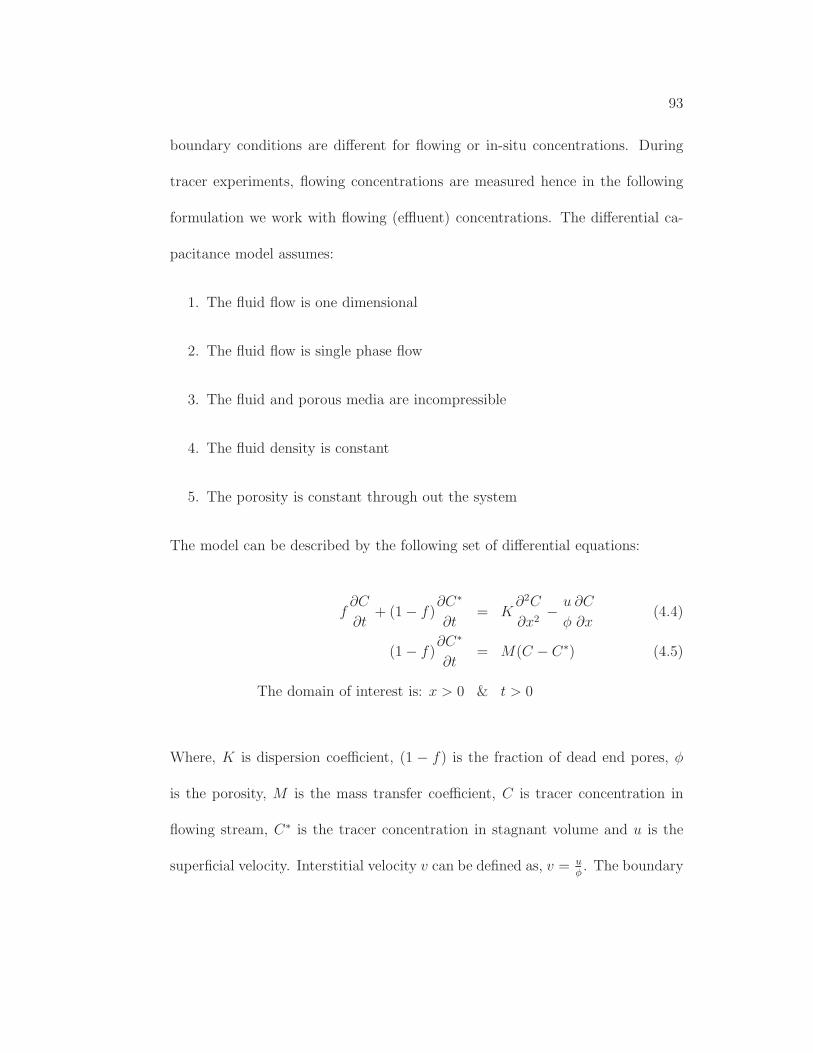
93

boundary conditions are different for flowing or in-situ concentrations. During

tracer experiments, flowing concentrations are measured hence in the following

formulation we work with flowing (effluent) concentrations. The differential ca-

pacitance model assumes:

1. The fluid flow is one dimensional

2. The fluid flow is single phase flow

3. The fluid and porous media are incompressible

4. The fluid density is constant

5. The porosity is constant through out the system

The model can be described by the following set of differential equations:

f∂C

∂t+ (1− f)

∂C∗

∂t= K

∂2C

∂x2− u

φ

∂C

∂x(4.4)

(1− f)∂C∗

∂t= M(C − C∗) (4.5)

The domain of interest is: x > 0 & t > 0

Where, K is dispersion coefficient, (1 − f) is the fraction of dead end pores, φ

is the porosity, M is the mass transfer coefficient, C is tracer concentration in

flowing stream, C∗ is the tracer concentration in stagnant volume and u is the

superficial velocity. Interstitial velocity v can be defined as, v = uφ. The boundary

94

and initial conditions are:

C(0, t) = CBC

C(∞, t) = 0

C(x, 0) = CIC

C∗(x, 0) = CIC

CBC is injected concentration at the inlet (x=0) and CIC is the initial concentration

in the system at the start of the experiment (t=0). The governing and boundary

and initial conditions are made dimensionless as follows: x = xL, t = t

t0, t0 = L

v;

where v is the interstitial velocity v = uφand L is system length. Dimensionless

concentrations are defined as:

C =

(

C − CIC

CBC − CIC

)

and C∗ =

(

C∗ − CIC

CBC − CIC

)

Using the above mentioned dimensionless variables the governing equations be-

come:

f∂C

∂t+ (1− f)

∂C∗

∂t= NK

∂2C

∂x2− ∂C

∂x(4.6)

(1− f)∂C∗

∂t= NM(C − C∗) (4.7)

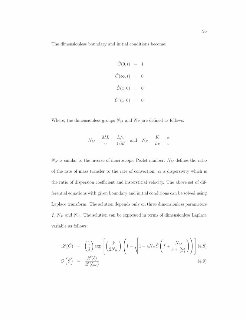
95

The dimensionless boundary and initial conditions become:

C(0, t) = 1

C(∞, t) = 0

C(x, 0) = 0

C∗(x, 0) = 0

Where, the dimensionless groups NM and NK are defined as follows:

NM =ML

v=

L/v

1/Mand NK =

K

Lv=

α

v

NK is similar to the inverse of macroscopic Peclet number. NM defines the ratio

of the rate of mass transfer to the rate of convection. α is dispersivity which is

the ratio of dispersion coefficient and insterstitial velocity. The above set of dif-

ferential equations with given boundary and initial conditions can be solved using

Laplace transform. The solution depends only on three dimensionless parameters

f , NM and NK . The solution can be expressed in terms of dimensionless Laplace

variable as follows:

L (C) =

(

1

s

)

exp

(

x

2NK

)

1−

√

√

√

√1 + 4NK S

(

f +NM

s+ NM

1−f

)

(4.8)

G(

S)

=L (c)

L (cBC)(4.9)

96

G(

S)

is the ratio of the Laplace transform of the effluent concentration to the

Laplace transform of the boundary condition. This is referred as the Transfer

function of the system. The resulting solution is numerically inverted into time

domain using the computer program of Hollenbeck (1998) which is based on

the algorithm of De Hoog, Knight and Stokes (1982). A plot of dimensionless

effluent concentration as function of model parameters is shown below in Figure

4.19. Figure 4.19 shows the effluent concentration as a function of pore volume

throughput for three distinct cases. When the flowing fraction is unity, effluent

concentration curve is symmetric around one pore volume with the concentration

of about 0.5 at one pore volume. This represents the case of the homogeneous

system with dispersion. For the second case, the value of flowing fraction is

0.1 and the value of NM = 0.1. In this scenario the effluent concentration rises

rapidly due to small flowing fraction at early times followed by a long tail which

represents small mass transfer between flowing and stagnant streams. For the

third case, the flowing fraction is 0.1 but the value of NM is three orders of

magnitude higher than that for the second case. In third case, due to strong

mass transfer between stagnant and flowing streams, the effluent concentration

curve does not exhibit a sharp rise and a long tail at larger times. A large value

of NM causes the effluent concentration curve to appear similar to the case of a

fictitious larger flowing fraction and small mass transfer. This is expected due

97

G H I J K LGG M HG M IG M JG M KG M LG M NG M OG M PG M Q H

t

c

R S T U V W X Y S V U T W X Z S T U VR S V U T W X Y S V U T W X Z S T U VR S V U T W X Y S V U T W X Z S T V U V

Figure 4.19: Effluent concentration versus pore volume throughput for a set ofdimensionless parameters

98

to the fact that the solution to the Coat’s and Smith model is not unique. The

problem of the non-uniqueness of the solution will be discussed in more detail in

the section describing the inversion process to obtain the fitted model parameters

from tracer flow experiments.

4.5 Recovery Efficiency and Transfer Between Flowing

And Stagnant Streams

Tracer flow analysis described in previous section can be complimented with

the help of recovery efficiency calculations. Recovery efficiency is defined as the

fraction of initial fluid in place displaced with injected tracer fluid.

Recovery Efficiency =∫ tmax

0

(

1− C)

dt

Hence, recovery efficiency can be plotted as a function of pore volume through-

put. When all of the initial fluid in place is displaced by injected tracer fluid,

the recovery efficiency approaches unity. Two sets of synthetic datasets shown in

figure 4.20 have the same value of flowing fraction and dispersivity (α) but dif-

ferent values of mass transfer group (NM). In first case even though the effluent

concentration approaches unity after 1.5 pore volumes, the recovery efficiency is

only 0.4 and hence most of initial fluid in place has not been replaced by injected

tracer fluid. Larger value of NM in second case results in significant mass transfer

between flowing and stagnant streams and recovery efficiency approaches unity

99

after about 2 pore volumes. Hence, recovery efficiency is an excellent measure of

the fraction of dead end pores contacted by displacing tracer fluid.

4.6 Parameter estimation from experimental data of tracer

concentration

Baker (1975) suggested that rather than transforming equation 4.8 into time

domain for the purpose of parameter estimation, the experimental data could be

transformed into the Laplace domain for obtaining fitted parameters using least

square curve fitting. The sum of squared errors can be defined as:

E =∑

s

∣

∣

∣

∣

∣

[

L (c)

L (cBC)

]

calc−[

L (c)

L (cBC

]

exptl

∣

∣

∣

∣

∣

2

(4.10)

The fitted parameters correspond to a set which minimizes the error defined by

equation 4.10. For parameter estimation, a computer program is written which

uses a built-in Matlab function for curve fitting based on Lavenberg-Marquardt

algorithm (Marquardt 1963).

To check the accuracy of curve fitting routine, synthetic experimental data is

generated for a known set of parameters. This synthetic data is treated as ex-

perimental data and fitted set of parameters are obtained. In another case, some

random noise is added to the synthetic data as shown in figure 4.21 and the

fitted set of parameters are obtained without any difficulty. When the value of

100

NM is large, the fitted parameters may not be correct due to the non-uniqueness

of the solution as shown in figure 4.23(A) where the inversion routine yields the

incorrect value of the model parameters used to create synthetic data. This hap-

pens because a large value of the mass transfer coefficient allows the exchange

between stagnant and flowing stream and resulting fitted parameters show ap-

parent higher value of flowing fraction. To obtain unique set of parameters, we

utilize the experimental data of effluent concentration at two different flow rates.

We further assume that mass transfer between stagnant and flowing streams is

dominated by diffusion process and the mass transfer coefficient does not depend

on the flow rate. The dispersion coefficient (K) is assumed to vary linearly with

the interstitial velocity (v). We use these additional constraints in the cost func-

tion of the parameter estimation algorithm and obtain the correct value of the

fitted model parameters as shown in figure 4.23(B).

4.7 Setup for the Tracer flow experiments and the data

acquisition protocol

The core holder for 1.5 inch diameter samples is Hassler type core holder. We have

adopted similar design for fabricating the flow setup for 3.5 inch diameter core

samples. Core holder for 3.5 inch diameter samples was custom fabricated in a

machine shop. High impact PVC is used to fabricate the end pieces and spacers

101

of the core holder while readily available PVC pipes are used for the outside

jacket of the core holder. A commercially avaialble core holder is used for 4.0

inch diameter samples. Based on the NMR T2 and permeability measurements,

the larger diameter samples are better candidates to study the connectivity of

vugs and to accurately characterize the pore structure. Sodium bromide is used

as non-adsorbing tracer in the experiments. For experiments, the initial tracer

concentration is 100 ppm and injected tracer boundary condition is 10, 000 ppm.

To measure the tracer concentration at outlet, a bromide ion sensitive electrode

is used in combination with a flow cell. The total Halide concentration (Cl− +

Br−) is kept at 0.15 M throughout the experiment to ensure the stable reading

of the electrode. The Bromide ion sensitive electrode and the flow cell enable us

to measure the tracer concentration with the help of a LabView data acquisition

module without collecting multiple effluent samples in batch and analyzing them

separately.

4.7.1 Reproducibility of tracer floods on core samples

Sodium Bromide is assumed to be a non adsorbing tracer in this study. Several

experiments were conducted to check the validity of this assumption. One core

plug (diameter of 1.5 inches) and one full core sample (diameter of 4.0 inches)

were used to run a series of tracer flow experiments and subsequently restored

to original initial condition by performing a restore flood of the initial condition.

102

Figure 4.24 shows the dimensionless effluent tracer concentration for the case of

10, 000 ppm flood followed by a 100 ppm restore flood at roughly same interstitial

velocity of 1.0 ft/day for a 1.5 inch diameter sample. We notice that the dimen-

sionless effluent concentration curves agree very well with each other within the

margin of experimental error. Figure 4.25 shows the effluent tracer concentration

for several floods at relatively higher interstitial velocity of about 7.0 ft/day for

a 4.0 inch diameter sample. The effluent concentration curves match very well

with one another for three different cases of 100 ppm and 10, 000 ppm floods.

These experiments demonstrate that Sodium Bromide does not adsorb to the

rock surface and no hysteresis is observed while restoring the core samples to

their initial conditions.

4.8 Tracer Flow Experiments

4.8.1 Validation with sandpacks and homogeneous rock system

Two types of sandpack systems are used in tracer experiments. The length of

each sandpack system is about one feet. The homogeneous sandpack is prepared

by using a single sand layer which has fairly uniform particle size distribution.

The heterogeneous sandpack consists of two layers of sand. The top layer sand is

of low permeability and the bottom layer sand has a permeability value which is

19 times that of the top layer. Each sand layer occupies half of the volume in the

103

sand pack. This system represents a case where the flowing fraction would be less

than one and there will be significant mass transfer between stagnant and flowing

streams. Figure 4.26 shows the plot of effluent Tracer concentration versus pore

volume throughput for both homogeneous and heterogeneous sandpacks. For

the homogeneous sandpack, the plot of effluent tracer concentration is symmetric

around one pore volume. However for the case of heterogeneous sandpack, Figure

4.26 shows early breakthrough of tracer which is a measure of smaller flowing

fraction. We also notice that effluent concentration increases slowly after an early

breakthrough. The flowing fraction for this case was interpreted to be about 0.65

from the effluent concentration data. Figure 4.27 shows the effluent concentration

and the recovery efficiency for homogeneous Silurian outcrop sample. We notice

that the effluent concentration curve is symmetric around one pore volume and

the flowing fraction (f) was estimated to be unity from the inversion algorithm.

4.9 Characterization of heterogeneous samples

Flow experiments were conducted on vuggy and fractured core plugs of 1.0 and

1.5 inch diameter and full sized cores of diameter 3.5 and 4.0 inches. Darcy’s law

was used to calculate the brine permeability based on the pressure drops across

the length of the core for the given set of flowrates. Despite being vuggy (as

confirmed in NMR spectrum), the permeability value for the majority of the 1.0

104

and 1.5 inch diameter was in the range of 0.5-6 mD. Only few 1.5 inch diameter

samples were found to have the permeability value of more than 10 mD. The

range of permeability for full sized cores was found to be 65-310 mD with the

exception of one 4.0 inch diameter sample whose permeability was calculated to

be 5 mD. To ensure the reliability of the tracer data, it is necessary that the dead

volume of the flow setup be much smaller than the pore volume of the sample.

Hence, the tracer flow experiments were not conducted on 1.0 inch diameter

samples because the pore volume of the plugs was smaller than the dead volume

of the setup. The following sections will describe the tracer characterization of

the different sized samples.

4.9.1 Tracer flow experiments on 1.5 inch diameter samples

In this section we discuss four of the tracer flow experiments conducted on dif-

ferent 1.5 inch diameter samples. One of the sample exhibits slow mass transfer

between flowing and stagnant streams while the other three samples exhibit much

higher mass transfer. Inverse of the mass transfer coefficient has units of time

and represents the timescale required to achieve equilibrium transport between

flowing and stagnant streams. Hence, an experiment conducted at a residence

time which is much smaller than the 1/M would show non-equilibrium effects

and strong dependence on the flow rate. The core samples exhibiting fast or

slow mass transfer are characterized based on the value of the inverse of the

105

mass transfer coefficient expressed in “days”. NMR T2 distribution which is a

representative of the pore size distribution is also measured and presented along

with tracer flow experiments for 1.5 inch diameter plugs. Sample 3V as shown

in figure 4.28 represents a rock sample with the flowing fraction (f) of 0.5, dis-

persivity (α) of 1 cm and 1/M of 0.17 days. This experiment was performed at

relatively faster flow rate of 15 ft/days. The corresponding residence time for this

experiment is much smaller than 1/M and thus the displacement of the tracer

from the flowing streams is not at equilibrium with the fluid in stagnant/dead

end pores. This behavior is confirmed by the plot of the recovery efficiency in

figure 4.28, where we see that after about 5 pore volumes only about 60% of the

initial fluid in place is recovered. Figure 4.29 represents the rock sample 1H with

the flowing fraction (f) of 0.2, dispersivity (α) of 0.8 cm and 1/M of 0.02 days or

about 30 minutes. The experiment shown was conducted at the relatively slow

flowrate of 1.4 ft/day. This corresponds to the residence time of about 3.2 hours

which is much higher than the value of 1/M . At such flowrate we should expect

the equilibrium between flowing and stagnant/dead end pores. Figure 4.29 also

shows the recovery efficiency for this flow experiment. We notice that after about

3 pore volumes the recovery efficiency reaches the value of unity and all of the

initial fluid in place has been displaced by the injected tracer fluid.

Samples 3V and 1H also differ drastically in their respective T2 relaxation

time spectrums. The T2 relaxation spectrum for sample 1H has a continuous

106

pore sizes distribution overlapping vugs, intermediate and small sized pores as

shown in figures 4.29. Figure 4.29 shows that the sample 3V on the other hand

does not have a significant overlap of relaxation times covering vugs, intermediate

and small sized pores. This could be the reason that the sample 1H can have

much higher value of the mass transfer coefficient in comparison to sample 3V.

The other two 1.5 inch diameter samples were drilled from the center of two

different 3.5 inch diameter cores. These core have the flowing fractions of 0.7

and 0.32 respectively. The value of 1/M is calculated to be of 0.26 and 0.34 days

respectively. The dispersivity (α) is calculated to be 1.2 and 1.7 cms respectively.

The plots of effluent concentration and recovery efficiency are shown in figures

4.30 and 4.31. In both cases, the value of the recovery efficiency reaches close

to unity after 5 pore volumes injected. Figures 4.30-4.31 also show the NMR T2

relaxation spectrum for these core plugs. For the samples exhibiting strong mass

transfer between flowing and stagnant streams, there is a significant overlap of

relaxation times corresponding to small and intermediate sized pores with the

relaxation times of the vugs.

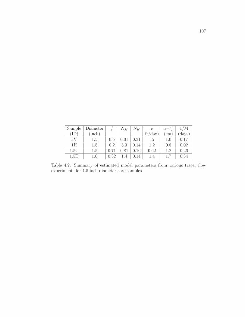
107

Sample Diameter f NM NK v α=Kv

1/M(ID) (inch) ft/day) (cm) (days)3V 1.5 0.5 0.01 0.31 15 1.0 0.171H 1.5 0.2 5.3 0.14 1.2 0.8 0.021.5C 1.5 0.71 0.81 0.16 0.62 1.2 0.261.5D 1.0 0.32 1.4 0.14 1.4 1.7 0.34

Table 4.2: Summary of estimated model parameters from various tracer flowexperiments for 1.5 inch diameter core samples

108

[ \ ] ^ _ `[[ a ][ a _[ a b[ a c \C d ed e

f g h i j kff l hf l jf l mf l ng

o pq rsturvwxyyz sz r{sw

| } ~ � � � � � } ~ � � � � � } ~ � ~ �| } ~ � � � � � } ~ � � � � � } � ~ � ~Figure 4.20: Plots of effluent concentration and recovery efficiency as a function ofpore volume throughput illustrating importance of mass transfer between flowingand stagnant streams

109

� � � � � � � � � � � ��

t

c � � � � � � � � � � � � � � � � � � � � � �� ¡ ¢ £ ¤ ¢ ¥ ¦ § ¨ ¢ ¨© ª « ¬ ® ¯ ª ° ¬ «® ± ª « ¬ °© ª « ¬ ²® ¯ ª ° ¬ «® ± ª ° ¬ «

Figure 4.21: A comparison of synthetic data with and without noise used forbenchmarking parameter estimation algorithm

³ ´ µ ¶ · ¸ ¹ º » ¼ ´ ³³³ ½ µ³ ½ ·³ ½ ¹³ ½ »ˆ

G(S

) ¾ ¿ À À Á Â Ã Ä ³ ½ ¸Å Æ Ä ³ ½ ¸Å Ç Ä ³ ½ µÈ É Ê Ê Á Ë ÀÃ Ä ³ ½ ¸Å Æ Ä ³ ½ ¸Å Ç Ä ³ ½ µÌ Í ¿ À ¿ Î Ï Ð Ñ Á Ò ÒÃ Ä ³ ½ ³ ¶Å Æ Ä ´Å Ç Ä ³ ½ ³ ´Ó Ô Í À Õ Á À ¿ Ë Ö Î À Î¾ ¿ À À Á Â È Ñ Ê × Á

Figure 4.22: A comparison of transfer function for experimental data and fittedcurve for parameter estimation

110

Ø Ù Ú Û Ü Ý Þ ß à á Ù ØØØ â ÚØ â ÜØ â ÞØ â à ÙS

G(S

)

ã ä å æ å ç è é ê ë ì ìí î Ø â Ø Ûï ð î Ùï ñ î Ø â Ø Ù ò ó ô ô ë õ æí î Ø â Ýï ð î Ù Ø Øï ñ î Ø â Ú ö å æ æ ë ÷í î Ø â àï ð î Ùï ñ î Ø â Úø ù ä æ ú ë æ å õ û ç æ çö å æ æ ë ÷ ò ê ô ü ë

Ø Ù Ú Û Ü Ý Þ ß à á Ù ØØØ â ÚØ â ÜØ â ÞØ â à ÙS

G(S

)

ã ä å æ å ç è é ê ë ì ìí î Ø â Ø Ûï ð î Ùï ñ î Ø â Ø Ù ò ó ô ô ë õ æí î Ø â Ýï ð î Ù Ø Øï ñ î Ø â Ú ö å æ æ ë ÷í î Ø â Ýï ð î Ù Ø Øï ñ î Ø â Úø ù ä æ ú ë æ å õ û ç æ ç Ùø ù ä æ ú ë æ å õ û ç æ ç Úö å æ æ ë ÷ ò ê ô ü ë Ùö å æ æ ë ÷ ò ê ô ü ë ÚFigure 4.23: Comparison of fitted model parameters using the inversion routinewhen (A) Data at one flowrate is used and (B) When data at two flow rates isused

111

ý þ ÿ � � �ýý � ÿý � �ý � �ý � �þ

� �C � � � � � � � � � � � ��

Figure 4.24: Effluent concentration versus pore volume throughput for 100 ppmand 10,000 ppm floods for similar values of the flowrates

� � � � � � � � � � � � � �� !� � "� � #�

PV

C

� � � $ $ % & ' � " ( ) * + , - .� � � $ $ % & " � # ( ) * + , - .� � / � � � $ $ % & ' � ' ( ) * + , - .

Figure 4.25: Effluent concentration versus pore volume throughput for 100 ppmand 10,000 ppm floods for several values of the flowrates

112

0 0 1 2 3 3 1 2 400 1 40 1 50 1 60 1 73

8 9

c

: ; < = > = ? = ; @ A B C ? D E C F G: = H = I ; > = ? = ; @ A B C ? D E C F G

Figure 4.26: Effluent concentration versus pore volume throughput for homoge-neous and heterogeneous sandpacks

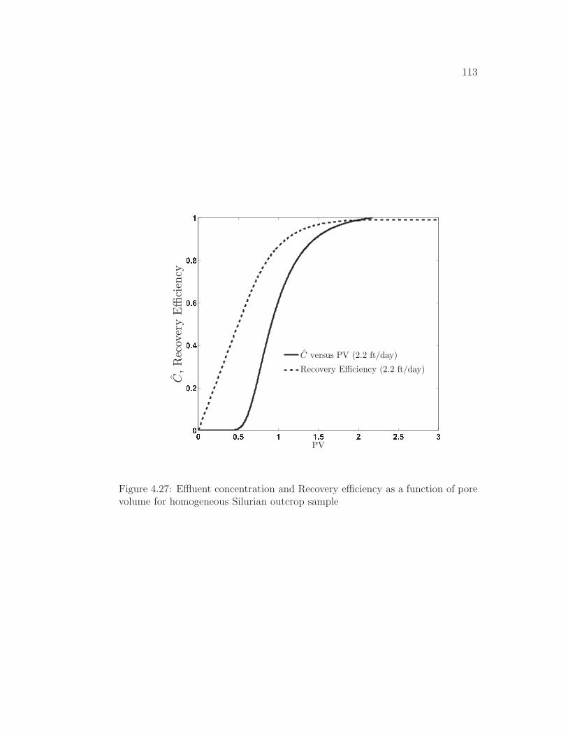
113

J J K L M M K L N N K L OJJ K NJ K PJ K QJ K RM

PV

C,R

ecov

ery

Effi

cien

cy

C versus PV (2.2 ft/day)

Recovery Efficiency (2.2 ft/day)

Figure 4.27: Effluent concentration and Recovery efficiency as a function of porevolume for homogeneous Silurian outcrop sample

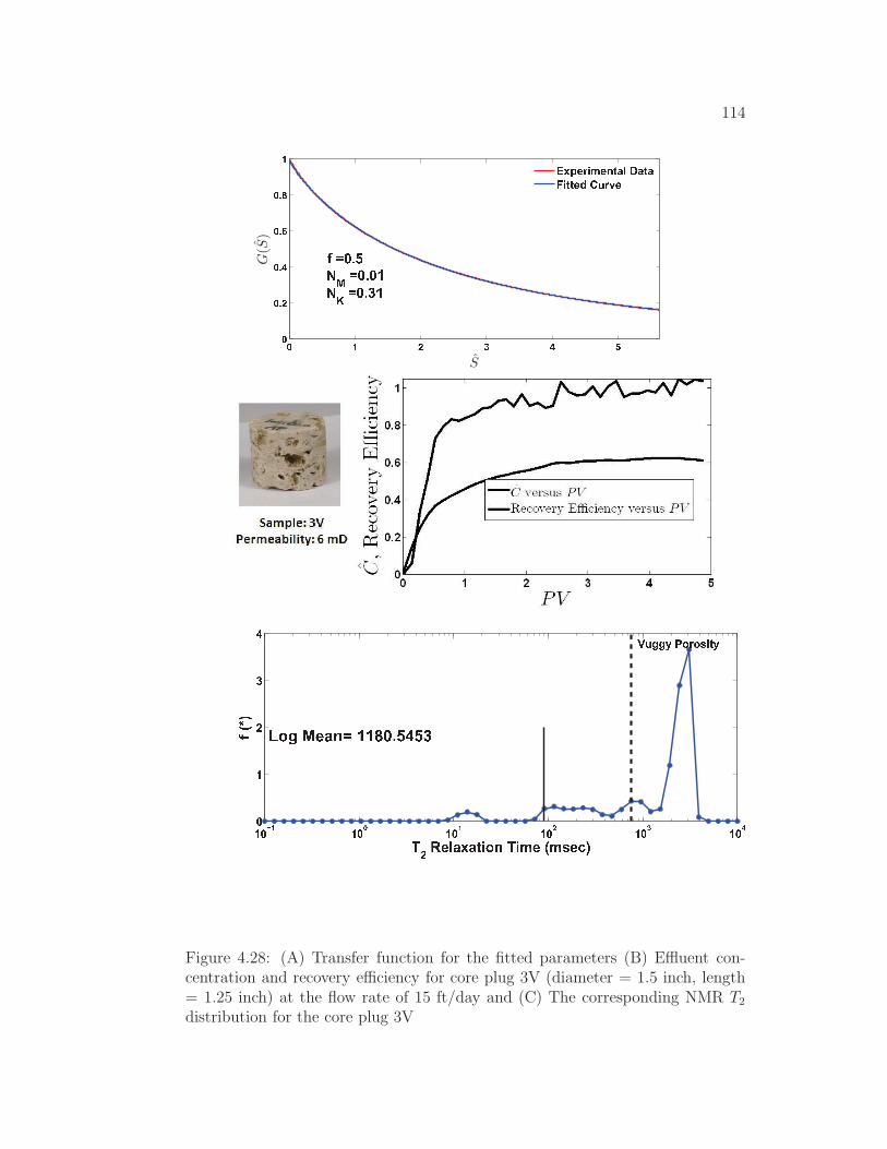
114

S T U V W XSS Y US Y WS Y ZS Y [ TS

G(S

) \ ] ^ _ `a b ] ^ _ ^ ca d ] ^ _ e cf g h i j k l i m n o p q o n or k n n i s t u j v i

w x y z w x { w x z w x | w x } w x ~xw��

� � � � � � � � � � � � � � � � ��

¡¢£¤ ¥ ¦ ¦ § ¨ © ª © « ¬ §

Figure 4.28: (A) Transfer function for the fitted parameters (B) Effluent con-centration and recovery efficiency for core plug 3V (diameter = 1.5 inch, length= 1.25 inch) at the flow rate of 15 ft/day and (C) The corresponding NMR T2

distribution for the core plug 3V

115

® ® ¯ ° ± ± ¯ ° ² ² ¯ ° ³ ³ ¯ ° ´ ´ ¯ ° °®® ¯ ²® ¯ ´® ¯ µ® ¯ ¶±S

G(S

) \ ] ^ _ · ^ `a b ] ` _ ea d ] ^ _ c ¸f g h i j k l i m n o p q o n or k n n i s t u j v i

¹ º » ¼ ¹ º ½ ¹ º ¼ ¹ º ¾ ¹ º ¿ ¹ º Àºº Á Âº Á Ãº Á Äº Á Å ¹Æ Ç È É Ê Ë Ì Í Î Ï Ð Ñ Ò Î Ó

Ô Â Õ Ê Ö Ë × Ë Ø Ù Ç Ì Ô Ù Ú Ê Û Ú Ü Ê Ý Þßàáâ ã ä å å æ ç è é è ê ë ì æ

Figure 4.29: (A) Transfer function for fitted parameters (B) Effluent concen-tration and recovery efficiency for core plug 1H (diameter = 1.5 inch, length =2.25 inch) at the flow rate of 1.4 ft/day and (C) The corresponding NMR T2

distribution for the core plug 1H

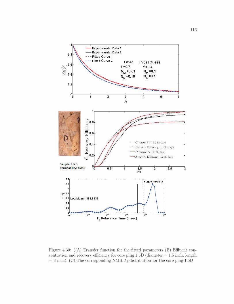
116

í î ï ð ñ ò óíí ô ïí ô ñí ô óí ô õ îS

G(S

) ö ÷ ø ø ù úû ü ý þ ÿ� � ü ý þ � �� ü ý þ � � � � ÷ ø ÷ � � ù � �û ü ý þ � � ü ý þ �� ü ý þ �� î� � � � � � � � � � � � � � � � ï� � � � � � � � � � � î� � � � � � � � � � � ï

� ! " � # � " � $ � % � & ' ( ' ) ' * ' +�� ' (� ' ) , - . / 0 1 2 3 4 5 6 7 5 8 4 9: ; < = > ? @ ? A B C D : B E = F E G = H IJKLM N O P P Q R S T S U V W Q

Figure 4.30: ((A) Transfer function for the fitted parameters (B) Effluent con-centration and recovery efficiency for core plug 1.5D (diameter = 1.5 inch, length= 3 inch), (C) The corresponding NMR T2 distribution for the core plug 1.5D

117

X Y Z [ \ ] ^XX _ ZX _ \X _ ^X _ ` YS

G(S

)

a b c c d ef g h i j kl m g n i ol p g h i n q r s b c b t u v w d x xf g h i n jl m g h i h yl p g h i nz { | d } b ~ d s c t u � t c t nz { | d } b ~ d s c t u � t c t ka b c c d e � w } � d na b c c d e � w } � d k

� � � � � � � � � � � � � � � � �� PV

C,R

ecov

ery

Effi

cien

cy





� � � � � � � � � � � � � � � � � � �� ¡ ¢ £ ¤ ¥ ¦ § � ¨ © ª « ¬ « ® ¯ ° § ® ± © ² ± ³ © ´ µ¶·¹ º » ¼ ¼ ½ ¾ ¿ À ¿ Á Â Ã ½

Figure 4.31: (A) Transfer function for the fitted parameters (B) Effluent concen-tration and recovery efficiency for core plug 1.5C (diameter = 1.5 inch, length =3.5 inch), (C) The corresponding NMR T2 distribution for the core plug 1.5B

118

4.10 Flow experiments on full sized cores

As discussed earlier, the permeability of the majority of the small sized core plugs

(1.5 and 1.0 inch diameter) was in the range of 0.5-6 mD with the exception of

few samples. The majority of these samples showed existence of vuggy porosity

as shown in NMR T2 relaxation. These small plugs were drilled from oil bearing

rock of the reservoir whose effective permeability is of the order 5 darcy. This

clearly shows that the vugs are non-touching thereby not enhancing the value of

the permeability significantly. The size of the vugs in rock samples is of the order

of few millimeters as the surface vugs are visible by the naked eye. Some of the

vugs are larger than a centimeter. Hence, the diameter of the small plugs is not

large enough to experience the enhancement of the permeability value due to the

vugs/fractures networks.

Hence larger diameter samples (3.5 inches and 4.0 inches) may be a better can-

didate to conduct experiments to understand these complex heterogeneous sys-

tems. Larger diameter samples offer another advantage while conducting Tracer

flow experiments. The pore volume of the larger diameter rocks is at least 10

times larger than the dead volume of the flow apparatus due to flow lines and

the flow cell for the electrode. Smaller relative dead volume for larger diameter

rock samples reduces artifacts like dispersion/mixing experienced during the flow

lines and the flow cell. The ISCO pumps are used to displace the tracer fluid

119

through the rock sample. The fluctuations in the flow rates are more pronounced

at relatively smaller flow rates (less than 1 ml/hr) needed for smaller sized core

plugs. Hence, using larger diameter core plugs improves the quality of the data

acquisition resulting in more accurate estimates of the fitted parameters during

tracer flow experiments.

Figure 4.32 shows the transfer function for the fitted parameters for three

different 3.5 inch diameter rock samples. The calculated values of the 1/M are

2.1 days, 4.3 days and 0.63 days for 3.5B, 3.5C and 3.5D respectively. The sample

3.5D exhibits strong mass transfer as is evidenced in the recovery efficiency shown

in figure 4.33. A 4.0 inch diameter sample (4.0B) was found to have strong mass

transfer even at the displacement rates of 12 ft/day. The value of 1/M for the

sample 4.0B was calculated to be 0.1 days.

Figure 4.34 on the other hand shows the effluent concentration and recovery

efficiency for the rocks samples exhibiting small mass transfer (1/M= 2.1 and

4.3 days). Figure 4.33 shows the effect of displacement rates (interstitial veloc-

ity) on mass transfer between flowing and stagnant streams. For sample 3.5B,

the calculated value of the 1/M is 2.1 days. Experiments were conducted for

three different interstitial velocities (21 ft/day, 1.8 ft/day and 0.36 ft/day). As

the interstitial velocity is reduced to less than 1 ft/day, we notice a significant

increase in the mass transfer between flowing and stagnant streams as evidenced

by enhanced recovery efficiency shown in figure 4.34

120

Ä Å Æ Ç È É ÊÄÄ Ë ÆÄ Ë ÈÄ Ë ÊÄ Ë ÌÅS

G(S

) Í Î Ï Ï Ð ÑÒ Ó Ä Ë È ÔÕ Ö Ó Ä Ë È ÅÕ × Ó Ä Ë Å Ì Ø Ù Î Ï Î Ú Û Ü Ý Ð Þ ÞÒ Ó Ä Ë ÅÕ Ö Ó Ä Ë ÅÕ × Ó Ä Ë Åß à á Ð â Î ã Ð Ù Ï Ú Û ä Ú Ï Ú Åß à á Ð â Î ã Ð Ù Ï Ú Û ä Ú Ï Ú ÆÍ Î Ï Ï Ð Ñ å Ý â æ Ð ÅÍ Î Ï Ï Ð Ñ å Ý â æ Ð Æ

ç è é ê ë ì íçç î éç î ëç î íç î ïè

S

G(S

) ð ñ ò ò ó ôõ ö ç î ÷ èø ù ö ç î è ÷ø ú ö ç î è û ü ý ñ ò ñ þ ÿ � � ó � �õ ö ç î ê ëø ù ö ç î ç ÷ ëø ú ö ç î è� � � ó � ñ � ó ý ò þ ÿ � þ ò þ è� � � ó � ñ � ó ý ò þ ÿ � þ ò þ éð ñ ò ò ó ô � � ó èð ñ ò ò ó ô � � ó é

í í ô ò î î ô ò ï ï ô ò ð ð ô ò ñíí ô ïí ô ñí ô óí ô õ îS

G(S

)

� � � � � �� í ô ò ñ � � í ô ñ ï � � í ô ï ñ � � � � � � � � � � � �� í ô î � � í ô í î � � í ô î� � � � � � � � � � � � � � � � î� � � � � � � � � � � � � � � � ï� � � � � � � � � � � î� � � � � � � � � � � ï

Figure 4.32: Transfer functions for the fitted parameters for 3.5B, 3.5C and 3.5Drock samples

121

� � � � � � � � �� C

,R

ecov

ery

Effi

cien

cy

PV





� � � � � � � � � � � � �� !� � "� � # �

PV

C,R

ecov

ery

Effi

cien

cy





Figure 4.33: Effluent concentration and Recovery efficiency for the cases whenstrong mass transfer is observed. (A) Sample 3.5D with 1/M = 0.6 days and (B)Sample 4.0B with 1/M = 0.1 days

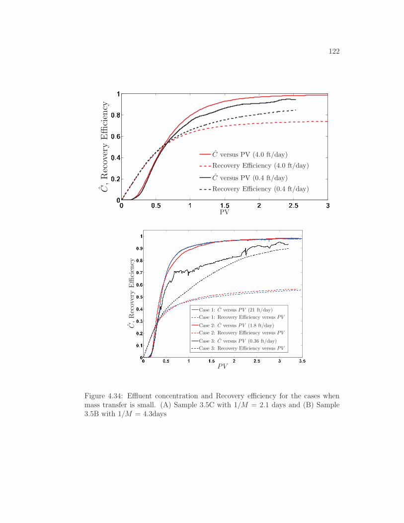
122

$ $ % & ' ' % & ( ( % & )$$ % ($ % *$ % +$ % ,'C

,R

ecov

ery

Effi

cien

cy

PV





- - . / 0 0 . / 1 1 . / 2 2 . /-- . 0- . 1- . 2- . 3- . /- . 4- . 5- . 6- . 7 0

PV

C,R

ecov

ery

Effi

cien

cy

Case 1: C versus PV (21 ft/day)

Case 1: Recovery Efficiency versus PV

Case 2: C versus PV (1.8 ft/day)


Case 3: C versus PV (0.36 ft/day)


Figure 4.34: Effluent concentration and Recovery efficiency for the cases whenmass transfer is small. (A) Sample 3.5C with 1/M = 2.1 days and (B) Sample3.5B with 1/M = 4.3days

123

After estimating unique model parameters from tracer flow experiments for

a known sample, the effluent concentration and the recovery efficiency can be

calculated as a function of pore volume throughput for various displacement rates

as shown in figure 4.35. We find that at high displacements rates only fraction of

dead end pores is contacted and the recovery is poor. As displacement rates are

decreased we find an optimum rate at which recovery efficiency is significantly

improved and reducing the displacement rates further are not useful. Experiments

to characterize the pore structure in the laboratories should be conducted at flow

rates which corresponds to NM value of 1.0 or higher to ensure enough exchange

between flowing and stagnant streams.

Estimated model parameters from tracer flow experiments are used to analyze

different regimes of mass transfer. The regime of small mass transfer corresponds

to the case when the value of dimensionless group for mass transfer is much

smaller than unity (NM < 1). In this regime effluent concentration/recovery

efficiency versus pore volume throughput curves are strongly dependent on in-

terstitial velocity. The regime of strong mass transfer corresponds to the case

when the value of dimensionless group for mass transfer is much greater than

unity (NM > 1). In the regime of strong mass transfer there is no dependence

of insterstitial velocity on effluent concentration/recovery efficiency curve. Table

4.3 presents a summary of fitted values of the parameters characterizing several

core samples. Some of these well characterized samples will be used to perform

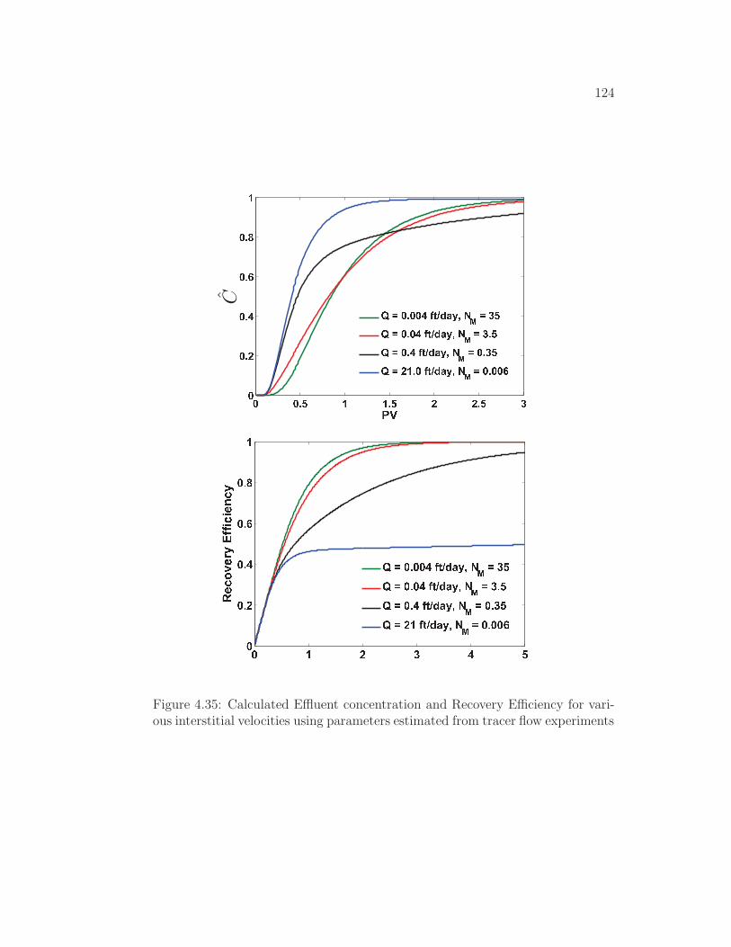
124

8 8 9 : ; ; 9 : < < 9 : =88 9 <8 9 >8 9 ?8 9 @;

A BC C D 8 9 8 8 > E F G H I J K L M D = :C D 8 9 8 > E F G H I J K L M D = 9 :C D 8 9 > E F G H I J K L M D 8 9 = :C D < ; 9 8 E F G H I J K L M D 8 9 8 8 ?

N O P Q R SNN T PN T RN T UN T VOW XYZ[X\]__ Y` XaY] b c N T N N R d e f g h i j k l c Q Sb c N T N R d e f g h i j k l c Q T Sb c N T R d e f g h i j k l c N T Q Sb c P O d e f g h i j k l c N T N N U

Figure 4.35: Calculated Effluent concentration and Recovery Efficiency for vari-ous interstitial velocities using parameters estimated from tracer flow experiments

125

Sample Diameter f NM NK v α=Kv

1/M(ID) (inch) ft/day) (cm) (days)3.5B 3.5 0.47 0.41 0.15 0.36 1.6 2.123.5C 3.5 0.71 0.17 0.19 0.4 1.7 4.33.5D 3.5 0.54 0.42 0.24 1.1 2.1 0.634.0A 4.0 0.64 0.61 0.14 1.1 2.7 0.934.0B 4.0 0.73 3.1 0.23 1.05 1.7 0.1

Table 4.3: Summary of estimated model parameters from various tracer flowexperiments for full core samples

the dynamic adsorption experiments to quantify the loss of surfactant to the rock

surface during the displacement process.

4.11 Static and Dynamic adsorption of surfactant

To evaluate the loss of the surfactant on rock, both static and dynamic exper-

iments are performed. The static test is done with centrifuge tubes using the

crushed powder of the rock sample. The dynamic experiments will be performed

in the presence of Sodium Bromide tracer to compare the breakthrough of the

surfactants that of the non-adsorbing tracer. The tracer concentration will be

recorded using an ion sensitive electrode and batch samples of the effluent will

be collected at regular intervals to be analyzed separately.

A blend of 4:1 weight ratio (active material) of Neodol 67-7PO sulfate (N67)

and C15-18 internal olefin sulfonate (IOS) from Stepan is used to study both

126

static and dynamic adsorption behavior on the rocks samples of interest. The

NI blend is selected because it has already been tested on Yates and Midland

farm fields. Both static as well as dynamic adsorption tests will be carried out

at room temperature and with the background salinity 1 wt% NaCl. Both of the

Neodol 67-7PO sulfate (N67) and C15-18 internal olefin sulfonate (IOS) are an-

ionic surfactants and hence the total surfactant concentration of the NI blend can

be accurately determined by Potentiometric titration with a cationic surfactant

such as Benzethonium Chloride (Hyamine) or Tego.

4.11.1 Static adsorption of surfactant on the crushed rock powder

The static adsorption experiments were performed as follows. A rock sample was

crushed into a homogeneous powder form and the BET surface area of the powder

was found to be 1.5 m2/gm. The known quantity (2 gms) of this rock powder was

mixed with 10 ml of the NI blend surfactant solution of various concentrations in

centrifuge tubes. The resulting mixture was shaken vigorously using a rotating

shaker system for 24 hours. The following day, the samples were centrifuged at

4000 rpm for at least 25 minutes. The supernatant solution from the centrifuge

tubes was carefully taken out and analyzed for the change in concentration of the

total surfactant.

The equilibrium surfactant concentrations, that is the concentration of the su-

pernatant solution were determined by potentiometric titration. Since the surface

127

m m n m o m n p m n p o m n qm n rm n sm n t pp n pp n qp n uv w xv w y

z { | } ~ } � � } | � � | � � � � � � � � � � � � � � � � � � } � � � � � � �� ¡ ¢ £ ~ � � ¤ ¥ } � ¦ � � | § ¦ � ¤ ¨ � ¥ ¤ � � � ¤ � � � ©

Figure 4.36: Adsorption on NI blend on crushed powder rock with BET area of1.5 m2/gm

area of the crushed rock powder is determined by BET adsorption, by comparing

the initial and equilibrium surfactant concentration, the amount of surfactant

adsorbed on the surface can be obtained as shown in figure 4.36. The total ab-

sorbant capacity of the powder can be calculated from the pleatau region and is

evaluated to be 1.12 mgm2 . In next section, the dynamic adsorption experiments

will be described and the loss of surfactant will be calculated.

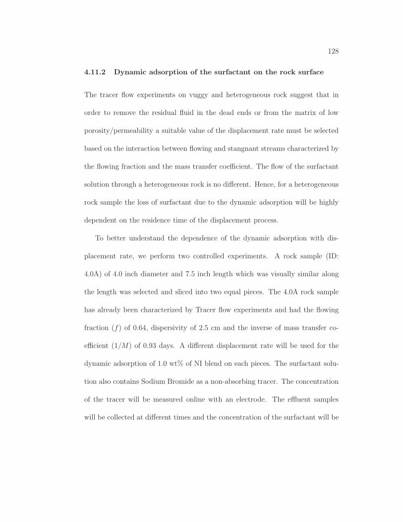
128

4.11.2 Dynamic adsorption of the surfactant on the rock surface

The tracer flow experiments on vuggy and heterogeneous rock suggest that in

order to remove the residual fluid in the dead ends or from the matrix of low

porosity/permeability a suitable value of the displacement rate must be selected

based on the interaction between flowing and stangnant streams characterized by

the flowing fraction and the mass transfer coefficient. The flow of the surfactant

solution through a heterogeneous rock is no different. Hence, for a heterogeneous

rock sample the loss of surfactant due to the dynamic adsorption will be highly

dependent on the residence time of the displacement process.

To better understand the dependence of the dynamic adsorption with dis-

placement rate, we perform two controlled experiments. A rock sample (ID:

4.0A) of 4.0 inch diameter and 7.5 inch length which was visually similar along

the length was selected and sliced into two equal pieces. The 4.0A rock sample

has already been characterized by Tracer flow experiments and had the flowing

fraction (f) of 0.64, dispersivity of 2.5 cm and the inverse of mass transfer co-

efficient (1/M) of 0.93 days. A different displacement rate will be used for the

dynamic adsorption of 1.0 wt% of NI blend on each pieces. The surfactant solu-

tion also contains Sodium Bromide as a non-absorbing tracer. The concentration

of the tracer will be measured online with an electrode. The effluent samples

will be collected at different times and the concentration of the surfactant will be

129

measured by potentiometric titrations to obtain the breakthrough curves of the

NI blend.

Figure 4.37 shows the comparison of the effluent surfactant concentration with

that of the tracer for two displacement rates of 11.12 ft/day and 0.125 ft/day

respectively. The first displacement rate was chosen such that the residence time

is very fast in comparison to the 1/M value of 0.93 days. We notice that there is

very little lag for the breakthrough of the surfactant. The slow flow of surfactant

corresponds to the residence time of 2.5 days for one pore volume. This should

allow enough time for the surfactant solution to come in equilibrium with the

fluid in stagnant volume. Finally the two surfactant floods are compared with

each other to show the lag of surfactant breakthrough for the slower flood.

The loss of the surfactant can be calculated using two methods. In first

method we take the difference in pore volumes for the 0.5 dimensionless value of

the tracer and surfactant concentrations. The second method is based on the mass

balance and we integrate the area of the curve for both of the surfactant solutions

and calculate the loss of surfactant. The specific surface area of the rock used in

the dynamic adsorption experiment is calculated to be 0.18 m2/gm from NMR

measurements. The specific surface area of the crushed powder used in static

adsorption experiments was found to be 1.5 m2/gm from BET measurements. In

order to compare the loss of the surfactant in the dynamic adsoprtion experiment

with that during static adsorption tests, the loss of surfactant is scaled with the

130

ª ª « ¬ « ¬ ® ® « ¬ ¯ªª « ª « ®ª « ¯ª « °ª « ¬ª « ±ª « ²ª « ³ª « ´

µ ¶·¸ ¹ º » ¼ ½ º¹ ¾ ¿ » À Á Â º Ã » ¼ ¿ » Ä ¿

Å Å Æ Ç È È Æ Ç É É Æ Ç Ê Ê Æ Ç ËÅÅ Æ ÈÅ Æ ÉÅ Æ ÊÅ Æ ËÅ Æ ÇÅ Æ ÌÅ Æ ÍÅ Æ ÎÅ Æ Ï È

Ð ÑÒÓ Ô Õ Ö × Ø ÕÔ Ù Ú Ö Û Ü Ý Õ Þ Ö × Ú Ö ß Ú

Figure 4.37: Adsorption of NI blend on a heterogeneous rock sample (A) Compar-ison of the surfactant fast flood with tracer (B) Comparison of the slow surfactantflood with tracer

131

Å Å Æ Ç È È Æ Ç É É Æ Ç Ê Ê Æ Ç Ë Ë Æ Ç ÇÅÅ Æ ÉÅ Æ ËÅ Æ ÌÅ Æ Î È

à áâã Ü Ý Õ Þ Ö × Ú Ö ß Ú Þ Û Ù Ù ä å È È Æ È É Þ Ú æ ä Ö ç èÜ Ý Õ Þ Ö × Ú Ö ß Ú Þ Û Ù Ù ä å Å Æ È É Ç Þ Ú æ ä Ö ç è

Figure 4.38: A comparison of fast and slow surfactant floods showing adsorptionof NI blend on a heterogeneous rock sample

132

Sample PV v Surfactant Loss of Surfactant Loss of Surfactant(ID) (ml) (ft/day) lag (PV) based on lag (mg/gm) mass balance (mg/gm)1 112 11.12 0.1 0.06 0.032 105 0.125 0.23 0.13 0.23

Table 4.4: Summary of both surfactant flood and loss of surfactant due to dy-namic adsorption

specific surface area of the rock. The rescaled value for the loss of surfactant in

dynamic adsorption experiments becomes 1.95 mg surfactant per gm of the rock.

This value is about same as that found for the static adsorption experiments.

133

Chapter 5

Conclusions and Future Work

5.1 Conclusions

5.1.1 Modeling internal field gradients for claylined pores

Chapter 3 described a modeling based approach to study the effect of internal

field gradients on the transverse relaxation. A two dimensional clay-flake model

was used to simulate transverse relaxation for claylined pore space. We found

that the Free induction decay (FID) in the presence of complex internal fields

can exhibit non-monotonically decreasing behavior. This behavior was explained

with the help of a test case involving no diffusion.

A simple two dimensional model is able to capture the spectrum of relaxation

regimes for transverse relaxation. The relaxation regimes can be classified on the

basic of the relative magnitudes of the different timescales for physical processes

such as τ, τ and τ ∗ω. No echo spacing dependence of transverse relaxation rate is

observed in motionally averaging regime. Localization and free diffusion regimes

show strong dependence of transverse relaxation on echo spacing. Relaxation

rates follow quadratic echo spacing dependence in free diffusion regime while less

134

than quadratic dependence on echo spacing is observed for localization regime. A

power-law dependence on echo-spacing is observed for crossover from one regime

to another.

5.2 Pore structure of vuggy carbonates

5.2.1 NMR Chracterization

The photographs of the core samples as well as NMR results suggest that these

carbonate rocks are very heterogeneous. In some cases, vugs contribute the most

to the porosity while in other smaller pores are dominant. Samples taken within

the proximity of 3 inches exhibit very different T2 relaxation time spectrum. The

majority of the samples show small value of permeability and the correlation

is very poor with the value of T2 Log Mean with the permeability by using the

current existing correlations. Brecciated samples having large solution vugs yields

relatively higher value of permeabilities in the laboratory experiments. NMR T2

relaxation spectrum can be used to calculate the distribution of porosity between

vugs and other smaller sized pores. The distribution of the surface area of the

pore space can also be calculated by with the help of the surface relaxivity. It is

found that the samples representing the reservoir rock have much higher surface

area in comparison to outcrop samples.

135

5.2.2 Characterization of the pore space by Tracer Analysis

Flow experiments suggested that the permeability of the rock samples is size

dependent. Smaller size samples (1.0 inch and 1.5 inches diameter) have the

permeability in the range of 0.5−6 mD. The range of permeability is 65−330 for

large diameter samples (3.5 inch and 4.0 inch diameter) samples. Both 3.5 inch

and 4.0 inch diameter samples have similar values of the permeabilities which are

about two orders of magnitude higher than that for smaller core plugs.

Tracer flow experiments were conducted to understand the effect of the het-

erogeneities due to the presence of vugs and fractures. It was found that only

a fraction of pore space form interconnected pathways for the passage of the

displacing fluid. The rest of the pore space is part of dead end pores and/or stag-

nant volume. Mass transfer is governing mechanism for transport across flowing

and stagnant streams. The timescale of mass transfer for some heterogeneous

samples was found to be in several days. The assumption of the equilibrium be-

tween flowing and stagnant streams will be broken during fast displacement rate

experiments resulting in poor recovery efficiency.

A control experiment for the dynamic adsorption was designed and conducted

for two order of magnitude different displacement rates. It was found that for very

small displacement rates 0.125 ft/day, the loss of the surfactant due to dynamic

adsorption is similar to that found in the static adsorption experiments.

136

5.3 Future Work

5.3.1 Dynamic adsorption model for heterogeneous systems

The simplest realistic model to describe the surfactant adsorption in porous media

is the so-called convection-dispersion model with linear adsorption with local

concentration (Gabbanelli, Grattoni and Bidner 1987). This type of approach

assumes that the adsorption isotherm can be approximated with a constant slope

over the range of concentration. This model can be solved analytically however

the assumptions of no dead volumes and linear adsorption isotherm are not valid

for heterogeneous systems. We have shown that the differential capacitance model

of Coats and Smith (1964) is able to describe the pore structure of the vuggy

carbonates. We also know that the actual adsorption of the NI blend follows

a Langmuir type isotherm as shown in the previous chapter. Thus, we use a

model developed by (Bidner and Vampa 1989) which combines the Langmuir

type isotherm with the differential capacitance model of Coats and Smith (1964).

This model is defined by the following set of differential equations:

f∂C

∂t= −∂C

∂x+NK

∂2C

∂x2−NM

(

C − C∗

)

− Laf

J

[

C (1− Γ)−EΓ]

(5.1)

∂C∗

∂t=

NM

1− f

(

C − C∗

)

− La

J

[

C∗ (1− Γ∗)− EΓ∗

]

(5.2)

∂Γ

∂t=

1

J

[

C (1− Γ)− EΓ]

(5.3)

∂Γ∗

∂t=

1

J

[

C∗ (1− Γ∗)− EΓ∗

]

(5.4)

137

Where, C and C∗ are the normalized solute concentrations in the flowing phase

and in the stagnant volume. Γ and Γ∗ are the normalized chemical adsorption in

flowing phase and in the stagnant volume. This set of dimensionless equations is

characterized y six dimensionless groups.

1. f is the flowing fraction.

2. NK = KLv

is the the dimensionless group for dispersion which is the inverse

of the Peclet Numer (Pe).

3. NM = MLv

is the dimensionless group for mass transfer.

4. La = AwrQa

ΦC0is the Langmuir number, which measures the adsorptive ca-

pacity of the system.

5. E = k2k1C0

is the Kinetic adsorption number, which relates desorption and

adsorption rates

6. J = vLk1C0

is the Flow rate number, which relates convection and adsorption.

Where, k1 and k2 are kinetic rate constants of adsorption and desorption, Qa

is the total adsorbent capacity and Awr is the surface area of the rock per unit

volume of the rock.

The tracer flow experiments can provide the first three dimensionless group

characterizing the porous media. Total adsorbent capacity can be calculated from

138

the static adsorption experiments. If the kinetic rate constants for the adsorption

and desorption are known, this model can be numerical solved to determine the

loss of surfactant during dynamic flow experiments.

139

Appendix A

Manual on using bromide ion sensitive electrode in laboratory experiments

Introduction: This is a manual to use a combination type bromide ion sensitive

electrode (ISE). The electrode is manufactured by Analytical Sensors and

Instruments, Ltd. which is located in Sugarland, Texas. The electrode belongs to

the “43 series” of their ion sensitive electrode catalog. The electrode measures

total free bromide ion concentration in aqueous solution. The electrode is of

combination type hence a reference electrode is not needed. This particular

electrode is chosen because the electrode junction is located very close to the

sensing element and hence the electrode requires a small sample volume (about

0.5 ml) for measurements. According to the manufacturer, the electrode has a

shelf life of about 6 months to one year after which it should be replaced. The

typical response time for the electrode is between 10-30 seconds.

Analytical Sensors & Instruments also have a bromide ion sensitive electrode

from “12 series” which has 1) a faster response time 2) comes with an additional

sensing module and 3) the electrolyte solution can be refilled. However,

electrode junction is located farther from the sensing element and this electrode

requires larger amount of sample volume (about 2-3 ml) for measurement.

Operation: When the electrode is immersed in a given aqueous solution

containing free bromide ions, a DC voltage is generated which can be measured

with the help of a multi-meter or other data acquisition interfaces such as

LabView® data acquisition module. The range of the concentration of bromide

140

ion which can be measured is 0.4 ppm to 79,999 ppm. The electrode can be

used at temperatures from 0 to 80 OC. It is important to keep total ion

concentration same in all samples for consistent results. We achieve this by

adding sodium chloride in the solution while keeping total halide ion

concentration same for all of the samples. Presence of other ions in the solution

affects the accuracy of electrode. Table 1 gives the maximum allowable ratio of

other ions to bromide ions in the solution when concentrations are measured in

either moles/L or ppm.

S.

No.

Interfering

ion

Maximum Ratio

(when units are expressed

as moles/L)

Maximum Ratio

(when units are

expressed as ppm)

1 OH- 3 x 104 6.4 x 103

2 Cl- 400 180

3 I- 2 x 10-4 3.2 x 10-4

4 S-2 10-6 4.0 x 10-8

5 CN- 8 x 10-5 2.6 x 10-6

6 NH3 2 4.2 x 10-4

Table 1: List of maximum allowable concentration of interfering ions for

bromide electrode

Calibration of the electrode (Theory): The generated DC voltage from the

electrode follows Nernst relationship as described in the equation below:

Where: E0 is a constant, T is the absolute temperature, F is Faraday constant, n

is the valence of the ion and is the activity of bromide ion in solution. At 25OC

141

for a tenfold change of concentration, the change in millivolt reading should be

within 54 mV to 60 mV.

Calibration Procedure:

The calibrating samples are prepared using successive dilution method i.e.

diluting from the sample of highest concentration of bromide ion to make smaller

concentration solutions. The total molar concentration of Sodium Chloride and

Sodium Bromide is kept constant at 0.125 M for all samples. For samples of

increasing Br-1 concentration, the moles of Sodium Chloride are replaced by

those of Sodium Bromide such that total molar halide concentration remains

constant. The electrode response is faster if the total molar concentration of

halides in the samples is kept constant. During measurements, it should be

ensured that there are no air bubbles trapped between solution and the surface

of sensing element. It takes about 30-60 seconds to reach 90% of the electrode

response. The electrode reading reaches steady state in about 3-5 minutes.

Change of 0.05 mV per minute or less should be used as an empirical rule of

thumb to check steady state.

Figure 1 shows the plot of mV versus Br-1 concentration in parts per

million. We observe that for low concentration the plot deviates from Nernst

relationship. This happens because at low concentration of Br-1, the ratio of

concentration of Cl-1 to that of Br-1 is larger than maximum allowable ratio given in

table 1. We found that for 100-10,000 ppm concentration range (0.125 molar total

salinity), electrode follows Nernst relationship as described in figures 2 and 3. We

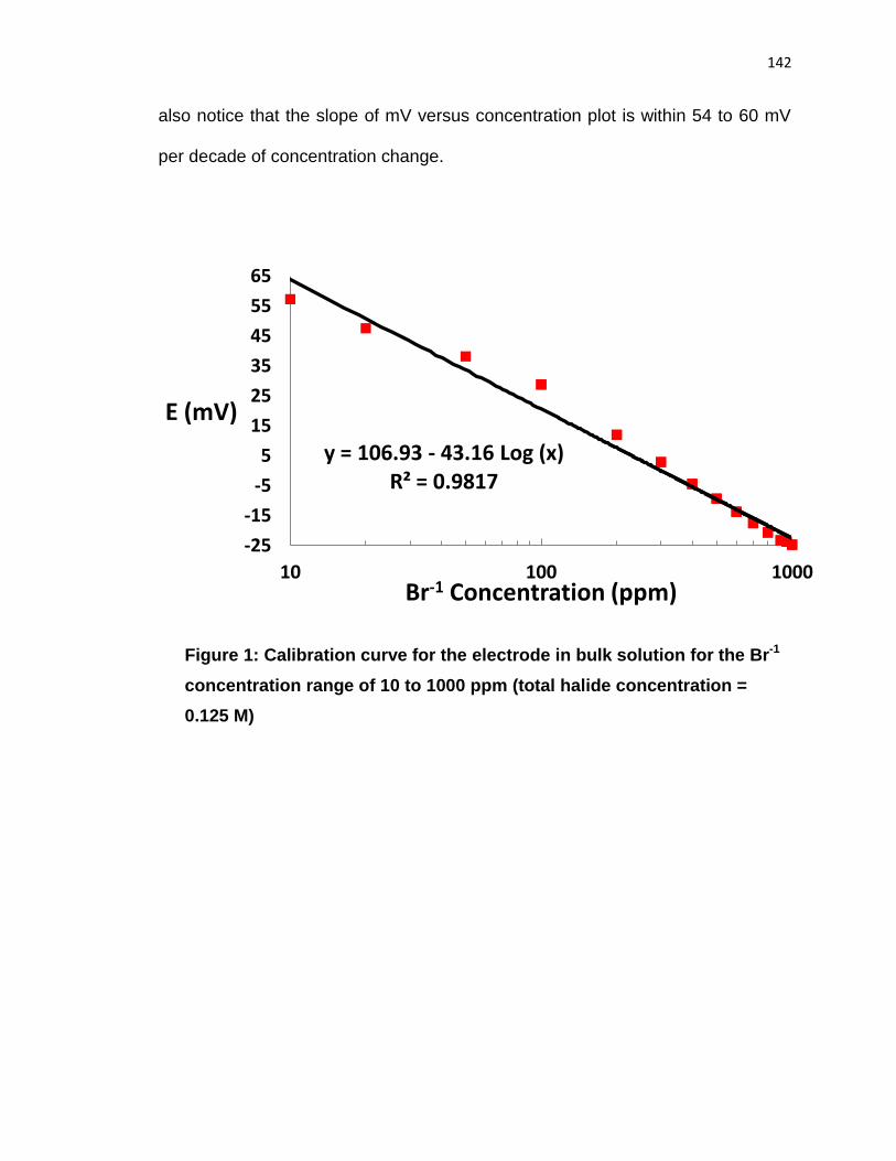
142

also notice that the slope of mV versus concentration plot is within 54 to 60 mV

per decade of concentration change.

Figure 1: Calibration curve for the electrode in bulk solution for the Br-1

concentration range of 10 to 1000 ppm (total halide concentration =

0.125 M)

y = 106.93 - 43.16 Log (x) R² = 0.9817

-25

-15

-5

5

15

25

35

45

55

65

10 100 1000

E (mV)

Br-1 Concentration (ppm)

143


concentration range of 100 to 1000 ppm (total halide concentration =

0.125 M)


concentration range of 100 to 10,000 ppm (total halide concentration =

0.125 M)

y = 136.19 -53.89 log (x) R² = 0.9994

-25

-15

-5

5

15

25

100 1000

E (mV)

Concentration (ppm)

y = 131.03 - 54.64 log(x) R² = 0.9998

-100

-80

-60

-40

-20

0

20

40

100 1000 10000

Concentration (ppm)

E (mV)

144

Conditioning of electrode prior to measurements and response time of the

electrode:

The operating manual suggests that electrode be first immersed in ionic strength

adjuster (ISA) for about 20-30 minutes before making measurements. Ionic

strength adjuster is 0.5 M Sodium Nitrate (NaNO3) solution. Figure 4 shows

transient response of the electrode when it was preconditioned using ISA versus

the case when it was not preconditioned prior to the measurement. Figure 4

shows that preconditioning electrode with ISA solution improves the response

time of the electrode.

Figure 4: Comparison of the transient response of the electrode when it was

preconditioned with ISA solution versus the case when it was not preconditioned

with ISA solution

Recommendations for the use of electrode:

-28

-26

-24

-22

-20

-18

-16 0 50 100 150 200 250 300

mV

Time (Seconds)

Electrode conditioned with ISA prior to measurement

Electrode not conditioned with ISA prior to measurement

145

To get consistent results when using the bromide electrode, one must follow

proper procedure. Start by placing the bromide in the ionic strength adjuster

(ISA) solution for 20-30 minutes followed by the lowest concentration for around

10 minutes. For accurate results, recalibrate bromide electrode after an

experiment on solutions where concentration is known. When placing the

electrode into a solution, ensure that there are no bubbles on the surface of the

sensing element.

The electrode should be rinsed with DI water in between static

measurements. While the measurement for the voltage of a static reading is

never completely stable, take your final measurement when the change in

electrode reading is less than 0.05 mV per minute. Electrode should never be left

immersed in de-ionized water. The electrode should be stored dry after

experiment and must be preconditioned before any use.

Data acquisition and alising: We use a LabView® data acquisition module to

read voltage from the electrode and write the data to a Microsoft excel file. The

typical range of sampling rate for LabView® module is 500-2000 Hz. LabView®

module uses an A/C power source at 60 Hz. Due to this, the electronic noise at

60 Hz is always added to the raw data read from the electrode. If proper care is

not taken during sampling and averaging of the raw data, signal aliasing can

occur which is shown in Figure 5. In this case we get an undulating noisy signal

in place of a steady value.

146

Figure 5: A plot showing strong signal aliasing

To further prove the existence of aliasing with 60 Hz A/C signal, we carry out

power spectrum analysis of the raw data at various sampling frequencies which

is shown in figure 6-9. We observe that a frequency of 60 Hz is always present in

the raw data collected from the electrode.

0 20 40 60 80 100 120

0

0.1

0.2

0.3

0.4

0.5

0.6

0.7

0.8

0.9

1

Time (sec)

C*

147

Figure 6: Power spectrum analysis of raw data collected at sampling rate of 5000 Hz


0 20 40 60 80 1000

2

4

6

8

10

Frequency (Hz)

Po

we

r

0 0.005 0.01 0.015 0.02 0.025 0.03 0.035 0.04 0.045 0.058

10

12

14

16

18

20

22

24

Time (sec)

mV

0 20 40 60 80 1000

2

4

6

8

10

Frequency (Hz)

Po

we

r

0 0.005 0.01 0.015 0.02 0.025 0.03 0.035 0.04 0.045 0.058

10

12

14

16

18

20

22

24

26

Time (sec)

mV

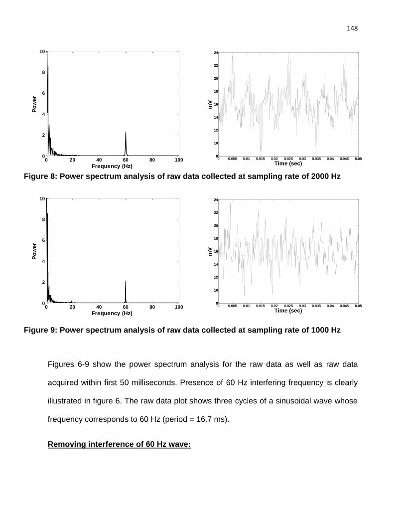
148



Figures 6-9 show the power spectrum analysis for the raw data as well as raw data

acquired within first 50 milliseconds. Presence of 60 Hz interfering frequency is clearly

illustrated in figure 6. The raw data plot shows three cycles of a sinusoidal wave whose

frequency corresponds to 60 Hz (period = 16.7 ms).

Removing interference of 60 Hz wave:

0 20 40 60 80 1000

2

4

6

8

10

Frequency (Hz)

Po

we

r

0 0.005 0.01 0.015 0.02 0.025 0.03 0.035 0.04 0.045 0.058

10

12

14

16

18

20

22

24

Time (sec)

mV

0 20 40 60 80 1000

2

4

6

8

10

Frequency (Hz)

Po

we

r

0 0.005 0.01 0.015 0.02 0.025 0.03 0.035 0.04 0.045 0.058

10

12

14

16

18

20

22

24

Time (sec)

mV

149

If data is acquired over a small sampling window, this may results in aliasing of 60 Hz

signal. This approach may also result in greater noise in sampled and averaged data.

Figure 11 shows the right methodology to gather sampled and averaged data. In order

to remove the effect of interfering frequency at 60 Hz, the raw data must be sampled

and averaged over a window of acquisition time much larger than the period of 60 Hz

wave as shown in figure 11.

150

Figure 10: Data acquired over a small sampling interval may result in aliasing

in data signal in certain situations

Figure 11: Data should be acquired over the whole range of sampling interval

and should be averaged to represent the sampling interval at mid point

There are two parameters which directly affect the sampled and averaged data.

A) Sampling rate (Hz): Sampling rate is the frequency at which LabView® module

communicates with the electrode. In our experiments, sampling rates of 1000 Hz

-2000 Hz were found to be adequate. Higher sampling rates results in large

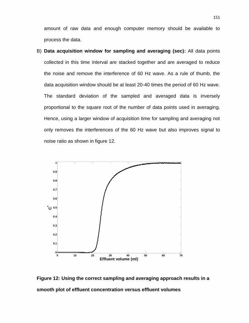
151

amount of raw data and enough computer memory should be available to

process the data.

B) Data acquisition window for sampling and averaging (sec): All data points

collected in this time interval are stacked together and are averaged to reduce

the noise and remove the interference of 60 Hz wave. As a rule of thumb, the

data acquisition window should be at least 20-40 times the period of 60 Hz wave.

The standard deviation of the sampled and averaged data is inversely

proportional to the square root of the number of data points used in averaging.

Hence, using a larger window of acquisition time for sampling and averaging not

only removes the interferences of the 60 Hz wave but also improves signal to

noise ratio as shown in figure 12.

Figure 12: Using the correct sampling and averaging approach results in a

smooth plot of effluent concentration versus effluent volumes

0 10 20 30 40 50 60 700

0.1

0.2

0.3

0.4

0.5

0.6

0.7

0.8

0.9

1

Effluent volume (ml)

C*

152

List of vendor websites:

1) Website of Analytical Sensors and Instruments:

http://www.asi-sensors.com

Contact person:

Alice Wong: [email protected]

2) Digital multi-meter can be purchased from any RadioShack store or from

following website:

http://www.multimeterwarehouse.com/digitalmultimeter.htm

3) The catalog of different types of sensors available at Analytical Sensor and

Instruments can be found at:

http://www.asi-sensors.com/ASI/docs/asicatalog.pdf

mailto:[email protected]

http://www.multimeterwarehouse.com/digitalmultimeter.htm

http://www.asi-sensors.com/ASI/docs/asicatalog.pdf

153

Bibliography

Anand, V. and Hirasaki, G. J. 2007a Diffusional coupling between microand macroporosity for NMR relaxation in sandstones and grainstones. Petro-physics 48 [No. 4] 289–307.

Anand, V. and Hirasaki, G. J. 2007b Paramagnetic relaxation in sandstones:Distinguishing T1 and T2 dependence on surface relaxation, internal gradi-ents and dependence on echo spacing. Journal of Magnetic Resonance 190

68–85.

Anjos, S. M. C., De Ros, L. F. and Silva, C. M. A. 2003 Chlorite authi-genesis and porosity preservation in the upper cretaceous marine sandstonesof the santos basin, offshore eastern Brazil, In: International Association ofSedimentologists Special Publication. Clay Mineral Cements in Sandstones34 291–316.

Appel, M., Freeman, J. J., Perkins, R. B. and Hofman, J. P. 1999Restriced Diffusion and Internal Field Gradients. in 40th Annual LoggingSymposium of the Society of Professional Well Log Analysts .

Baker, L. 1975 Effects of dispersion and dead-end pore volume in miscibleflooding. Soc. Pet. Eng. AIME, Pap 5632 50.

Bergman, D. J. and Dunn, K.-J. 1995a NMR of diffusing atoms in a periodicporous medium in the presence of a nonuniform magnetic field. Phys. Rev.E 52 [No. 6] 6516–6535.

Bergman, D. J. and Dunn, K. J. 1995b Self-diffusion in a Periodic Porous-medium With Interface Absorption. Physical Review E 51 [No. 4] 3401–3416.

Bidner, M. and Vampa, V. 1989 A general model for convection-dispersion-dynamic adsorption in porous media with stagnant volume. Journal ofPetroleum Science and Engineering 3 [No. 3] 267–281.

154

Bloch, S., Lander, R. and Bonnell, L. 2002 Anomalously High Poros-ity and Permeability in Deeply Buried Sandstone Reservoirs: Origin andPredictability. AAPG Bulletin 86 [No. 2] 301–328.

Borgia, G. C., Brown, R. J. S. and Fantazzini, P. 1995 Scaling of spin-echo amplitudes with frequency, diffusion coefficient, pore size, and suscepti-bility difference for the NMR of fluids in porous media and biological tissues.Phys. Rev. E 51 [No. 3] 2104–2114.

Brigham, W. 1974 Mixing equations in short laboratory cores. Soc. Pet. Eng.J 14 91–99.

Brooks, R. A., Moiny, F. and Gillis, P. 2001 On T-2-shortening by weaklymagnetized particles: The chemical exchange model. Magnetic Resonance inMedicine 45 [No. 6] 1014–1020.

Brown, R. J. S. and Fantazzini, P. 1993 Conditions for initial quasilinearT−1

2versus τ for Carr-Purcell-Meiboom-Gill NMR with diffusion and sus-

ceptibility differences in porous media and tissues. Phys. Rev. B 47 [No. 22]14823–14834.

Brownstein, K. R. and Tarr, C. E. 1979 Importance of classical diffusion inNMR studies of water in biological cells. Phys. Rev. A 19 [No. 6] 2446–2453.

Carr, H. Y. and Purcell, E. M. 1954 Effects of Diffusion on Free Precessionin Nuclear Magnetic Resonance Experiments. Phys. Rev. 94 [No. 3] 630–638.

Cerepi, A., Durand, C. and Brosse, E. 2002 Pore microgeometry analysisin low-resistivity sandstone reservoirs. Journal of Petroleum Science andEngineering 35 [No. 3-4] 205–232.

Chang, D., Vinegar, H., Morriss, C. E. and Straley, C. 1997 Effectiveporosity, producible fluid and permeability in carbonates from NMR logging.Log Analyst 38 [No. 2].

Chen, Q. and Song, Y. Q. 2002 What is the shape of pores in natural rocks?Journal of Chemical Physics 116 [No. 19] 8247–8250.

Claudine, D., Etienne, B. and Adrian, C. 2001 Effect of pore-lining chlo-rite on petrophysical properties of low-resistivity sandstone reservoirs. SPEReservoir Evaluation & Engineering, June 231–239.

Coats, K. and Smith, B. 1964 Dead-end pore volume and dispersion in porousmedia. Soc. Pet. Eng. J 4 [No. 1] 73–84.

155

De Hoog, F., Knight, J. and Stokes, A. 1982 An improved method fornumerical inversion of Laplace transforms. SIAM Journal on Scientific andStatistical Computing 3 357.

de Swiet, T. M. d. S. and Sen, P. N. 1994 Decay of nuclear magnetizationby bounded diffusion in a constant field gradient. The Journal of ChemicalPhysics 100 [No. 8] 5597–5604.

Dunn, K. J., Appel, M., Freeman, J. J., Gardner, J. S., Hirasaki,

G. J., Shafer, J. L. and Zhang, G. 2001 Interpretation of RestrictedDiffusion and Internal Field Gradients in Rock Data. Published in the Pro-ceedings of 42nd Annual Symposium of Society of Professional Well LogAnalysts, Houston, TX .

Fantazzini, P. and Brown, R. J. S. 2005 Initially linear echo-spacing de-pendence of I/T-2 measurements in many porous media with pore-scale in-homogeneous fields. Journal of Magnetic Resonance 177 [No. 2] 228–235.

Foley, I., Farooqui, S. A. and Kleinberg, R. L. 1996 Effect of paramag-netic ions on NMR relaxation of fluids at solid surfaces. Journal of MagneticResonance Series a 123 [No. 1] 95–104.

Gabbanelli, S., Grattoni, C. and Bidner, M. 1987 Miscible flow throughporous media with dispersion and adsorption. Advances in water resources10 [No. 3] 149–158.

Gillis, P. and Koenig, S. H. 1987 Transverse Relaxation of Solvent ProtonsInduced by Magnetized Spheres - Application to Ferritin, Erythrocytes, andMagnetite. Magnetic Resonance in Medicine 5 [No. 4] 323–345.

Gillis, P., Moiny, F. and Brooks, R. A. 2002 On T-2-shortening bystrongly magnetized spheres: A partial refocusing model. Magnetic Reso-nance in Medicine 47 [No. 2] 257–263.

Glasel, J. A. and Lee, K. H. 1974 Interpretation of Water Nuclear Magnetic-resonance Relaxation-times in Heterogeneous Systems. Journal of the Amer-ican Chemical Society 96 [No. 4] 970–978.

Grebenkov, D. S. 2007 Nuclear magnetic resonance restricted diffusion be-tween parallel planes in a cosine magnetic field: An exactly solvable model.Journal of Chemical Physics 126 [No. 10].

Gudbjartsson, H. and Patz, S. 1995 NMR diffusion simulation based onconditional random walk. Medical Imaging, IEEE Transactions on 14 [No.4] 636–642.

156

Hayes, J. B. 1970 Polytypism of chlorite in sedimentary rocks. Clays and ClayMinerals 18 [No. 5] 285–291.

Hidajat, I., Mohanty, K., Flaum, M. and Hirasaki, G. 2004 Studyof vuggy carbonates using NMR and X-Ray CT scanning. SPE ReservoirEvaluation & Engineering 7 [No. 5] 365–377.

Hollenbeck, K. 1998 INVLAP. M: A matlab function for numerical inversionof Laplace transforms by the de Hoog algorithm. [Online; accessed 05-July-2009].URL: http://www.isva.dtu.dk/staff/karl/invlap.htm

Hurlimann, M. D. 1998 Effective gradients in porous media due to suscepti-bility differences. Journal of Magnetic Resonance 131 [No. 2] 232–240.

Hurlimann, M. D., Helmer, K. G., Deswiet, T. M. and Sen, P. N.

1995 Spin Echoes in a Constant Gradient and in the Presence of SimpleRestriction. Journal of Magnetic Resonance, Series A 113 [No. 2] 260–264.

Kenyon, W. E. 1997 Petrophysical principles of applications of NMR logging.The Log Analyst 38 [No. 2] 21–43.

Kleinberg, R. L. and Horsfield, M. A. 1990 Transverse relaxation pro-cesses in porous sedimentary rock. J. Magn. Reson 88 [No. 9] 9–19.

Kleinberg, R. L., Kenyon, W. E. and Mitra, P. P. 1994 Mechanism ofNMR Relaxation of Fluids in Rock. Journal of Magnetic Resonance SeriesA 108 [No. 2] 206–214.

La Torraca, G. A., Dunn, K. J. and Bergman, D. J. 1995 Magneticsusceptibility contrast effects on NMR T2 logging. SPWLA 36th AnnualLogging Symposium 26–29.

Le Doussal, P. and Sen, P. N. 1992a Decay of nuclear magnetization bydiffusion in a parabolic magnetic field: An exactly solvable model. Phys.Rev. B 46 [No. 6] 3465–3485.

Le Doussal, P. and Sen, P. N. 1992b Decay of nuclear magnetization bydiffusion in a parabolic magnetic field: An exactly solvable model. Phys.Rev. B 46 [No. 6] 3465–3485.

Loren, J. D. and Robinson, J. D. 1970 Relationship between pore size andfluid matrix properties and NMR measurements. Transaction, AIME 249

268–278.

157

Lucia, F. 1999 Carbonate reservoir characterization. Springer Verlag,.

Marquardt, D. W. 1963 An Algorithm for Least-Squares Estimation of Non-linear Parameters. Journal of the Society for Industrial and Applied Mathe-matics 11 [No. 2] 431–441.

Mitra, P. P. and Sen, P. N. 1992 Effects of microgeometry and surface relax-ation on NMR pulsed-field-gradient experiments: Simple pore geometries.Physical Review B 45 [No. 1] 143–156.

Neuman, C. H. 1974 Spin echo of spins diffusing in a bounded medium. TheJournal of Chemical Physics 60 [No. 11] 4508–4511.

Palaz, I. and Marfurt, K. 1997 Carbonate seismology. Society of ExplorationGeophysicists,.

Peaceman, D. and Rachford Jr, H. 1955 The numerical solution ofparabolic and elliptic differential equations. Journal of the Society for In-dustrial and Applied Mathematics 28–41.

Ramakrishnan, T. S., Fordham, E. J., Venkataramanan, L., Flaum,

M. and Schwartz, L. M. 1999 New interpretation methodology basedon forward models for magnetic resonance in carbonates [C], Paper MMM.Annual Logging Symposium Transactions, Society of Petrophysicists WellLog Analysts .

Robertson, B. 1966 Spin-Echo Decay of Spins Diffusing in a Bounded Region.Physical Review 151 [No. 1] 273–277.

Rueslatten, H., Eidesmo, T., Lehne, K. and Relling, O. 1998 Theuse of NMR spectroscopy to validate NMR logs from deeply buried reservoirsandstones. Journal of Petroleum Science and Engineering 19 [No. 1] 33–43.

Sen, P. N. 2004 Time-dependent diffusion coefficient as a probe of geometry.Concepts in Magnetic Resonance 23 [No. 1] 1–21.

Song, Y., Lisitza, N. V., Allen, D. F. and Kenyon, W. E. 2002 Poregeometry and its geological evolution in carbonate rocks. Petrophysics 43

[No. 5] 420–424.

Song, Y. Q. 2000 Determining pore sizes using an internal magnetic field. Jour-nal of Magnetic Resonance 143 [No. 2] 397–401.

Song, Y. Q. 2001 Pore sizes and pore connectivity in rocks using the effect ofinternal field. Magnetic Resonance Imaging 19 [No. 3–4] 417–421.

158

Song, Y. Q., Ryu, S. G. and Sen, P. N. 2000 Determining multiple lengthscales in rocks. Nature 406 [No. 6792] 178–181.

Storvoll, V., Bjørlykke, K., Karlsen, D. and Saigal, G. 2002 Porositypreservation in reservoir sandstones due to grain-coating illite: a study ofthe Jurassic Garn Formation from the Kristin and Lavrans fields, offshoreMid-Norway. Marine and Petroleum Geology 19 [No. 6] 767–781.

Straley, C., Morriss, C. E., Kenyon, W. E. and Howard, J. J. 1991NMR in Partially Saturated Rocks: Laboratory Insights on Free Fluid In-dex and Comparison with Borehole Logs. SPWLA, 32nd Annual LoggingSymposium 1–25.

Straley, C., Morriss, C., Kenyon, W. and Howard, J. 1995 NMR inpartially saturated rocks: laboratory insights on free fluid index and com-parison with borehole logs. Log Analyst 36 40–56.

Sukstanskii, A. L. and Yablonskiy, D. A. 2002 Effects of Restricted Diffu-sion on MR Signal Formation. Journal of Magnetic Resonance 157 [No. 1]92–105.

Tarczon, J. C. and Halperin, W. P. 1985 Interpretation of NMR diffusionmeasurements in uniform- and nonuniform-field profiles. Phys. Rev. B 32

[No. 5] 2798–2807.

Torrey, H. C. 1956 Bloch Equations with Diffusion Terms. Phys. Rev. 104[No. 3] 563–565.

Toumelin, E., Torres-Verdın, C., Chen, S. and Fischer, D. 2003 Recon-ciling NMR measurements and numerical simulations: assessment of temper-ature and diffusive coupling effects on two-phase carbonate samples. Petro-physics 44 [No. 2] 91–107.

Trantham, J. C. and Clampitt, R. L. 1977 Determination of oil saturationafter waterflooding in an oilwet reservoir-The North Burbank Unit, Tract97 Project. J. Pet. Technol 491–500.

Valckenborg, R. M. E., Huinink, H. P., v. d. Sande, J. J. and

Kopinga, K. 2002 Random-walk simulations of NMR dephasing effectsdue to uniform magnetic-field gradients in a pore. Phys. Rev. E 65 [No. 2]021306.

Velde, B. 1995 Origin and Mineralogy of Clays: Clays and the Environment.Springer,.

159

Wayne, R. C. and Cotts, R. M. 1966 Nuclear-Magnetic-Resonance Study ofSelf-Diffusion in a Bounded Medium. Phys. Rev. 151 [No. 1] 264–272.

Weisskoff, R. M., Zuo, C. S., Boxerman, J. L. and Rosen, B. R. 1994Microscopic Susceptibility Variation and Transverse Relaxation - Theoryand Experiment. Magnetic Resonance in Medicine 31 [No. 6] 601–610.

Wilson, M. and Pittman, E. 1977 Authigenic clays in sandstones; recogni-tion and influence on reservoir properties and paleoenvironmental analysis.Journal of Sedimentary Research 47 [No. 1] 3–31.

Woessner, D. E. 1960 Self-diffusion measurements in liquids by the spin-echotechnique. Sci. Instrum 31.

Woessner, D. E. 1961 Effects of diffusion in nuclear magnetic resonance spin-echo experiments. J. Chem. Phys 34.

Woessner, D. E. 1963 NMR spin-echo self-diffusion measurements on fluidsundergoing restricted diffusion. The Journal of Physical Chemistry 67 [No.6] 1365–1367.

Worden, R. H. and Morad, S. 2003 Clay minerals in sandstones: controlson formation, distribution and evolution, In: International Association ofSedimentologists Special Publication. Clay Mineral Cements in Sandstones34 3–41.

Zhang, G. Q. and Hirasaki, G. J. 2003 CPMG relaxation by diffusionwith constant magnetic field gradient in a restricted geometry: numericalsimulation and application. Journal of Magnetic Resonance 163 [No. 1] 81–91.

Zhang, G. Q., Hirasaki, G. J. and House, W. V. 2001 Effect of InternalField Gradients on NMR Measurements. Petrophysics 42 [No. 1] 37–47.

Zhang, G. Q., Hirasaki, G. J. and House, W. V. 2003 Internal fieldgradients in porous media. Petrophysics 44 [No. 6] 422–434.

Zhang, Q. 2001 NMR Formation Evaluation: Hydrogen Index, Wettability andInternal Field Gradients. PhD Thesis .

Zielinski, L. J. and Hurlimann, M. D. 2005 Probing short length scales withrestricted diffusion in a static gradient using the CPMG sequence. Journalof Magnetic Resonance 172 [No. 1] 161–167.

Documents

Transverse Relaxation in Sandstones due to the eﬀect of