Transportation Research Part D - DLR Portalelib.dlr.de/115799/1/Hendricks-etal-TRD-2017.pdf · Quantifying the climate impact of emissions from land-based transport in Germany Johannes

Transportation Research Part D xxx (2017) xxx–xxx

Contents lists available at ScienceDirect

Transportation Research Part D

journal homepage: www.elsevier .com/ locate/ t rd

Quantifying the climate impact of emissions from land-basedtransport in Germany

http://dx.doi.org/10.1016/j.trd.2017.06.0031361-9209/� 2017 The Authors. Published by Elsevier Ltd.This is an open access article under the CC BY-NC-ND license (http://creativecommons.org/licenses/by-nc-nd/4.0/).

⇑ Corresponding author.E-mail address: [email protected] (J. Hendricks).

Please cite this article in press as: Hendricks, J., et al. Quantifying the climate impact of emissions from land-based transport in GeTransport. Res. Part D (2017), http://dx.doi.org/10.1016/j.trd.2017.06.003

Johannes Hendricks a,⇑, Mattia Righi a, Katrin Dahlmann a, Klaus-Dirk Gottschaldt a,Volker Grewe a,b, Michael Ponater a, Robert Sausen a, Dirk Heinrichs c, Christian Winkler c,Axel Wolfermann c,f, Tatjana Kampffmeyer d,g, Rainer Friedrich d, Matthias Klötzke e,Ulrike Kugler e

aDeutsches Zentrum für Luft- und Raumfahrt (DLR), Institut für Physik der Atmosphäre, Oberpfaffenhofen, GermanybDelft University of Technology, Faculty of Aerospace Engineering, Section Aircraft Noise & Climate Effects, Delft, NetherlandscDeutsches Zentrum für Luft- und Raumfahrt (DLR), Institut für Verkehrsforschung, Berlin, GermanydUniversity of Stuttgart, Institute for Energy Economics and the Rational Use of Energy (IER), Stuttgart, GermanyeDeutsches Zentrum für Luft- und Raumfahrt (DLR), Institut für Fahrzeugkonzepte, Stuttgart, GermanyfHochschule Darmstadt, University of Applied Sciences, Department of Civil Engineering, Darmstadt, Germanyg Statistisches Landesamt Baden-Württemberg, Stuttgart, Germany

a r t i c l e i n f o a b s t r a c t

Article history:Available online xxxx

Keywords:Regional transportEmissionsClimate changeClimate modelingTransport modelingGerman transport system

Although climate change is a global problem, specific mitigation measures are frequentlyapplied on regional or national scales only. This is the case in particular for measures toreduce the emissions of land-based transport, which is largely characterized by regionalor national systems with independent infrastructure, organization, and regulation. The cli-mate perturbations caused by regional transport emissions are small compared to thoseresulting from global emissions. Consequently, they can be smaller than the detection lim-its in global three-dimensional chemistry-climate model simulations, hampering the eval-uation of the climate benefit of mitigation strategies. Hence, we developed a new approachto solve this problem. The approach is based on a combination of a detailed three-dimensional global chemistry-climate model system, aerosol-climate response functions,and a zero-dimensional climate response model. For demonstration purposes, theapproach was applied to results from a transport and emission modeling suite, whichwas designed to quantify the present-day and possible future transport activities inGermany and the resulting emissions. The results show that, in a baseline scenario,German transport emissions result in an increase in global mean surface temperature ofthe order of 0.01 K during the 21st century. This effect is dominated by the CO2 emissions,in contrast to the impact of global transport emissions, where non-CO2 species make a lar-ger relative contribution to transport-induced climate change than in the case of Germanemissions. Our new approach is ready for operational use to evaluate the climate benefitof mitigation strategies to reduce the impact of transport emissions.� 2017 The Authors. Published by Elsevier Ltd. This is an open access article under the CC

BY-NC-ND license (http://creativecommons.org/licenses/by-nc-nd/4.0/).

rmany.

http://creativecommons.org/licenses/by-nc-nd/4.0/

http://dx.doi.org/10.1016/j.trd.2017.06.003

http://creativecommons.org/licenses/by-nc-nd/4.0/

mailto:[email protected]


http://www.sciencedirect.com/science/journal/13619209

http://www.elsevier.com/locate/trd


2 J. Hendricks et al. / Transportation Research Part D xxx (2017) xxx–xxx

1. Introduction

Recent changes of the Earth’s climate can be attributed to anthropogenic emissions, and these changes are expected tofurther increase in the future (e.g., Stocker et al., 2013). Emissions from the transport sectors (land-based transport, shipping,and aviation) significantly contribute to this effect (e.g., Fuglestvedt et al., 2008; Eyring et al., 2010; Lee et al., 2010; Sausen,2010; Uherek et al., 2010; Sausen et al., 2012). This is of particular relevance in view of comparatively large growth rates ofthese sectors. Climatically active components of transport emissions include (i) the long-lived greenhouse gas CO2; (ii) short-lived trace gases, in particular nitrogen oxides (NOx = NO + NO2), carbon monoxide (CO), and volatile organic compounds(VOC), which can induce changes in the concentration of the greenhouse gases ozone (O3) and methane (CH4); as well as(iii) aerosol particles (e.g., soot) and aerosol precursor gases (e.g., SO2 or the aforementioned NOx and VOC), which can causeimportant modifications of clouds and radiation.

Many concepts for mitigating climate change have been developed. These include numerous strategies to reduce theemissions from the transport sectors (see Kahn Ribeiro et al., 2007, for a review). Climate change is a global problem. How-ever, specific measures frequently apply on regional or national scales only. This is the case in particular for land-basedtransport, which is largely characterized by regional or national systems with independent infrastructure, organization,and regulation. As an example, in 2007 the German government initiated an integrated energy and climate program(German Federal Ministry for the Environment, Nature Conservation, Building and Nuclear Safety, 2007). One of the centralobjectives of this initiative has been a significant reduction of the national transport emissions. This is intended to beachieved by a number of measures including a CO2 strategy for passenger cars, an expansion of the biofuels market, aCO2-based reform of vehicle taxes, energy labeling of passenger cars, as well as modifications of the German heavy goodsvehicle toll. Such measures influence not only the emissions of CO2, but also the amount of other, co-emitted species. Hence,evaluating possible climate benefits of such measures requires a quantification of the climate impact of the regionaltransport emissions taking into account all climate-relevant emission components. An important facet of the problem is thateven local mitigation measures may induce a large-scale to global climate response.

Global climate models are the central tools for assessing anthropogenic climate change since cause-effect relations can bestudied in detail. In addition, such models allow projections of future climate based on different emission scenarios (e.g.,Stocker et al., 2013). Many studies have focused on modeling climate effects of emissions from the global transport systems(e.g., Lauer et al., 2007; Hoor et al., 2009; Skeie et al., 2009; Dahlmann et al., 2011; Lund et al., 2012; Peters et al., 2012, 2013;Righi et al., 2013, 2015, 2016). Also the climate benefits of specific mitigation options for global transport have been mod-eled, particularly for aviation (e.g., Ponater et al., 2006; Frömming et al., 2012; Grewe et al., 2014) and international shipping(e.g., Lauer et al., 2010; Righi et al., 2011). However, corresponding studies of the global climate benefits of regional measuresto reduce emissions of land-based transport are lacking.

Different types of climate models have been used for quantifying the global climate impacts of the different species emit-ted. While long-lived greenhouse gases (e.g., CO2) are well-mixed in the atmosphere and, consequently, show a nearly homo-geneous spatial distribution, short-lived species (e.g., ozone or particles) are mostly characterized by large spatial variationsand their climate effects, even the global mean response, can depend on the location of the corresponding emissions (e.g.,Joshi et al., 2003; Berntsen et al., 2005, 2006; Shindell et al., 2010). This implies that three-dimensional global atmosphericchemistry-climate models are needed to simulate these effects. Performing such simulations for longer time periods (e.g.,centuries) would cause extreme computational expenses. Therefore, such model studies are typically performed for selectedperiods of a few years only (e.g., Gottschaldt et al., 2013; Righi et al., 2013).

The commonway to quantify perturbations of short-lived species induced by a specific emission source is to compare twothree-dimensional simulations, one with and one without these emissions. On the basis of radiative transfer calculations,these perturbations are then translated into a radiative forcing (RF) metric, which represents their impact on the Earth’s radi-ation budget and can be interpreted as an indicator for the strength of the resulting global climate change (e.g., Myhre et al.,2013). A positive global mean radiative forcing results in a warming of climate, whereas a negative forcing induces a cooling.Once the radiative forcing has been quantified, it can be used as the basis for further climate change calculations, for exam-ple, for estimating the corresponding change in global mean surface temperature.

In the case of long-lived greenhouse gases a different approach is favored. The quasi-homogeneous spatial distribution ofthese compounds has the advantage that zero-dimensional climate response models can be applied to simulate the atmo-spheric concentration perturbations induced by specific emission sources as well as the resulting global climate effects(e.g., Sausen and Schumann, 2000). Due to their numerical efficiency, such models allow for larger numbers of simulationsin order to analyze many different emission scenarios or mitigation options. These models also enable long-term simulationsand projections, which are necessary to consider the long residence times and the resulting atmospheric accumulation oflong-lived species, such as CO2, which can reside in the atmosphere for centuries.

Climate response models are based on response functions derived from simulations with detailed climate models. Theseresponse functions provide both changes in greenhouse gas concentrations and changes in global mean surface temperatureper unit of emission. Therefore, they are suitable for quantifying the effects of even small local CO2 emission sources. Hence,the global climate effects induced by the CO2 emissions of regional transport systems can be determined and, consequently,the effects of regional emissions in different future scenarios can be compared. In contrast, a fundamental problem ariseswhen effects of emissions of short-lived species are assessed with three-dimensional models. The global perturbations

Please cite this article in press as: Hendricks, J., et al. Quantifying the climate impact of emissions from land-based transport in Germany.Transport. Res. Part D (2017), http://dx.doi.org/10.1016/j.trd.2017.06.003


J. Hendricks et al. / Transportation Research Part D xxx (2017) xxx–xxx 3

induced by regional emissions are small compared to those resulting from global emissions. As a consequence, the modeledperturbations can be smaller than the detection limits in global three-dimensional chemistry-climate model simulations(e.g., Deckert et al., 2011; Righi et al., 2013) and the transport-induced climate effects cannot be quantified.

For the assessment of gas-phase chemical perturbations, this problem can be solved by neglecting any feedbacks of theperturbations to other atmospheric processes in the model (Deckert et al., 2011). This significantly reduces the noise (arisingfrom natural variability) and, hence, increases the signal-to-noise ratios of the transport-induced perturbations. Based on thechemical perturbations quantified by this method, the corresponding radiation and climate effects can be derived in subse-quent calculations using, for example, off-line radiative transfer and climate response models. However, a decoupling of pro-cesses as described by Deckert et al. (2011) is not suitable for the quantification of aerosol effects since aerosol-inducedmodifications of clouds, that is, coupling processes, are major mechanisms of anthropogenic climate change. This severelyhampers the assessment of the climate effects of regional emission sources.

Hence, for a complete assessment of the global climate impact of regional land-based transport emissions, different mod-eling techniques need to be combined and, with regard to aerosol effects, new methods need to be designed. In the presentstudy, we developed such an overall approach, covering the effects of the whole suite of different emission components. Themethod is based on a combination of (i) a three-dimensional global chemistry-climate model system to quantify ozone dis-tribution changes and their radiative impact; (ii) a set of newly derived aerosol-climate response functions to quantify theradiative forcing of aerosol perturbations directly from aerosol and aerosol precursor emissions; and (iii) a climate responsemodel to simulate the concentration changes of the long-lived greenhouse gases CO2 and CH4 and the resulting radiativeimpacts. The latter model has the additional capability to translate the radiative effects of all species into changes of the glo-bal mean surface temperature.

For demonstration purposes, the approach was applied to the results of a transport and emission modeling suite, whichhad been designed to assess the present-day and possible future transport activities in Germany as well as the resultingemissions of climate-relevant species. The development and application of the approach were part of the DLR project VEU(Verkehrsentwicklung und Umwelt, i.e., transport development and environment; www.dlr.de/VEU/en/). VEU has the objec-tive to analyze German transport activities and their environmental impacts. The applied model framework, including trans-port, emission, and atmospheric models, enables an evaluation of mitigation strategies by modeling the full cause-effectchain ranging from transport demand, over transport activity and emissions, to the resulting climate effects. Although theapplication example focused on the effects of transport emissions in Germany, the methods are in principle applicable toother regions, too.

In addition to their climate impact, transport-induced air pollutants can affect human health (e.g., Pope and Dockery,2006; Chow et al., 2006). However, we focus on the climate effects here and refrain from discussing air pollution aspectssince this would be beyond the scope of the present paper.

This article is organized as follows: Section 2 describes the methodology to quantify the climate impacts of regional emis-sion sources as well as the methods to derive emissions of the German transport system. The section starts with a briefmethodological summary which provides basic technical information for those readers who are particularly interested inthe application results and who intend to focus their attention on Section 3, where the results are presented and discussed.Section 4 summarizes the main conclusions of our study.

2. Models and methodology

2.1. Methodological overview

To evaluate the climate impact of transport emissions, changes in the atmospheric concentrations of the individualclimate-relevant species as well as the corresponding effects on radiation and, finally, climate need to be assessed. The atmo-spheric modeling suite applied here to achieve this is shown in Fig. 1 together with the data flow between its differentcomponents.

To quantify transport effects on atmospheric ozone, the global three-dimensional chemistry-climate model system EMAC(ECHAM5/MESSy atmospheric chemistry model; Section 2.2.1) is applied in the so-called quasi chemistry transport model(QCTM) configuration. That means that feedbacks of the chemical perturbations to other atmospheric processes areneglected, which enhances the signal-to-noise ratio. The model is used to calculate the transport-induced ozone modifica-tions and the resulting radiative forcing. An additional result of these model calculations is the transport-induced change inmethane lifetime caused by modified chemical sinks. This information is applied in a subsequent modeling step (see below)to quantify the corresponding change in the methane concentration and the resulting radiative forcing. For a more detaileddescription of the QCTM application in the present study, we refer to Section 2.2.1.

To quantify the radiative forcing of aerosol perturbations induced by regional transport emissions, we derived a set ofclimate response functions which allow the calculation of aerosol radiative forcing directly from the emissions. These func-tions are based on detailed three-dimensional aerosol-climate model calculations also performed with the EMAC model sys-tem. By varying the total European anthropogenic emissions of aerosols and aerosol precursor gases in these simulations, thedependence of the aerosol radiative forcing on the emission strength was quantified and corresponding response functionswere fitted to the results. This enabled us to quantify the radiative forcings of aerosol perturbations induced by specific


http://www.dlr.de/VEU/en/


Fig. 1. Schematic overview of the atmospheric modeling approach and the data flow between the different tools applied. The aerosol-climate responsefunctions, the chemistry-climate model EMAC (in QCTM mode), and the climate response model AirClim are applied to calculate the radiative forcings (RF)of changes in aerosols, ozone (O3), methane (CH4), and CO2 induced by transport emissions. AirClim further simulates the resulting climate effects expressedas the change in global mean surface temperature DT. Ds(CH4) denotes the change of methane lifetime induced by transport emissions.


transport activities in the European area, even if these perturbations are below the detection limit in the three-dimensionalsimulations. A detailed description of this approach is provided in Section 2.2.2.

For calculating the transport-induced changes in the concentrations of CO2 and CH4 as well as the corresponding radiativeforcings, we apply the climate response model AirClim (Section 2.2.3). While the CO2-related modifications are derived fromthe CO2 emissions, the CH4-related changes are quantified on the basis of the CH4 lifetime modifications simulated withEMAC in the QCTM setup. Since the radiative forcings of the CO2 and CH4 concentration changes depend on the backgroundconcentrations of these species, AirClim employs time-dependent background concentrations according to observations forthe past. To account for the future development of the CO2 and CH4 background as well, appropriate scenarios have to beassumed. In the applications of the present study, we take into account three different future scenarios to assess the sensi-tivity of our results to different assumptions about future developments. The chosen background scenarios are described inSection 2.2.4.

The final outcome of the three methods described above are radiative forcings. Additional processing is necessary toassess the climate effects resulting from these radiation budget perturbations. This cannot be accomplished by simply takinginto account atmospheric processes alone since climate change also involves modifications of ocean temperatures whichtake place on long time-scales (decades). Computationally expensive coupled atmosphere-ocean models are required to sim-ulate the temporal and spatial details of this effect. Such models cannot be applied for a large number of simulations oftransport-induced perturbations. Therefore relations between radiative forcing and parameters describing the associated cli-mate change (e.g., change in global mean surface temperature) were established in previous studies and are exploited withinthe AirClim model, in a final simulation step to calculate temperature changes resulting from the radiative forcings of theindividual species (ozone, aerosol, CO2, and CH4). The details of this approach are described in Section 2.2.4.

In the demonstration application within the VEU project, the modeling approach described above was used to quantifythe climate effects of the emissions from the transport activities within Germany. The focus was on land-based transportincluding road transportation, railways, and inland navigation. For the description of the German transport system withinVEU, transport models were applied which are suitable for assessing present-day and possible future transport activities.Fig. 2 provides a flow chart of the transport modeling methodology followed here. Based on socio-economic input data, pas-senger and freight transport demand is modeled to generate origin-destination matrices. These matrices are then used toassign transport demand to the traffic network for calculating transport activity in terms of link flows, that is, the numberof vehicle movements per time between network nodes. In this manner, transport activities for different vehicle types arequantified. In addition, the future development of the passenger car fleet composition is explicitly modeled, in order to takeinto account the penetration of new technologies into the vehicle market. For a detailed description of the transport mod-eling approach, we refer to Section 2.3.1. The emissions of climate relevant species from the German transport system arequantified by combining the modeled transport activity data with emission factors for the respective vehicle types. Detailsabout the chosen emission factors are provided in Section 2.3.2.

For the present study, a baseline scenario of the transport development in Germany between 2008 and 2030 was gener-ated. Transport activities and the resulting emissions were calculated for the years 2008, 2020, and 2030. Due to methodical



Fig. 2. Schematic overview of the transport and emission modeling approach.


issues described in Section 2.2.1, the atmospheric simulations, particularly of ozone and the methane lifetime change (QCTMsimulations), require information about all emission sources within Europe. Hence, the German transport emission datawere complemented by inventories of transport emissions of all other European countries (except for the European partof Russia) and corresponding Europe-wide anthropogenic non-transport emissions (Section 2.3.2).

Due to the long atmospheric residence time and the resulting accumulation and long-term climatic impact of CO2, thetime period from 2008 to 2030 is too short to perform an appropriate analysis of the climate effects. Longer time periodsneed to be analyzed to enable a fair comparison of the effects of short-lived species and long-lived greenhouse gases (Sec-tion 2.2.4). Hence, we expanded the time horizon of our analysis to the year 2100 and also took into account past transport-induced emissions back to 1850. To this end, the emission data generated for transport in Germany in the period from 2008to 2030 were complemented by corresponding data for the past, based on results of other studies. Since no information wasavailable about the emissions during parts of the considered time periods, appropriate assumptions were made in thesecases. For the years beyond 2030, constant emissions on the 2030 level were assumed. Details of these emission estimatesare described in Section 3.1. The results of the transport and emission modeling suite and the corresponding results of mod-eling the climate effects of the German transport emissions are described in Sections 3.1 and 3.2, respectively.

2.2. Atmospheric modeling

2.2.1. Transport-induced ozone changesTo quantify the effect of transport emissions on atmospheric ozone, we employ the global three-dimensional chemistry-

climate model system EMAC (Jöckel et al., 2006). It consists of a physical climate model (ECHAM5) coupled with a number ofsubmodels which are needed to simulate atmospheric chemistry. In this combination, the physical climate model simulatesatmospheric dynamics (e.g., winds, temperature), the hydrological cycle, and the atmospheric radiation budget. The addi-tional submodels describe specific processes in the chemical species’ life cycle, such as emissions, gas and liquid-phasechemical transformations, or deposition to the surface.

To enable the quantification of small perturbations, we apply this model framework in the QCTM configuration (Deckertet al., 2011). Using this model setup, the feedbacks of atmospheric chemistry perturbations to other atmospheric processes,in particular to radiation and dynamics, are neglected by considering prescribed concentrations of radiatively active gases inthe radiative transfer calculations, rather than driving the radiation by chemical concentrations calculated on-line. Thisimplies that the chemical perturbations do not change atmospheric dynamics (i.e., weather and climate), thus reducingthe ‘noise’ in the modeled transport effects and enabling the quantification even of small transport-induced chemistry




perturbations. For the applications of the present study, the model was operated in the configuration described as ‘base con-figuration’ by Gottschaldt et al. (2013), but using different emission inventories as input.

To describe the possible future development of global anthropogenic emissions, we consider the Representative Concen-tration Pathways (RCPs) emission data (van Vuuren et al., 2011) generated in support of the Fifth Assessment Report of theIntergovernmental Panel on Climate Change (IPCC; e.g., Stocker et al., 2013). For the QCTM simulations of our demonstrationapplication, we analyzed the differences in total annual emissions of short-lived species in the different European countriesas represented by the RCPs and as quantified in VEU. We then chose the RCP scenario (RCP8.5) that is closest to the VEUprojections, assuming that this scenario shows the highest consistency to the VEU scenario also with regard to the futuredevelopment of short-lived species emissions outside Europe. To allow for maximum consistency with the VEU scenariowithin Europe, we embedded the European VEU emissions into the global data set. This was achieved by scaling the RCPemission amounts of each constituent in the respective sectors and European countries to match the corresponding VEUemissions.

The effects of emissions from the transport sector on atmospheric ozone can be calculated by comparing two differentQCTM simulations, one including all emission sources and another one neglecting the emissions from the transport sector.This standard approach is referred to as the perturbation method (e.g., Grewe et al., 2012). For our demonstration applica-tion, this implies that simulations with and without German transport emissions were necessary. Although the numericalnoise is reduced significantly in the QCTM approach compared to simulations with the fully coupled model, some noise isstill inherent in the chemistry calculations and may complicate the quantification of the expectedly small signal resultingfrom the German emissions. To overcome this, we enhanced the transport-induced perturbation by simulating the ozonechange induced by the land-based transport emissions of all European countries (except for the European part of Russia),instead of focusing on the effect of German emissions only. The radiative forcing that results from this ozone change wasthen calculated according to Gottschaldt et al. (2013) from the differences of the radiative fluxes simulated in the two modelruns. We then estimated the radiative forcing resulting from German transport activities by downscaling the European effectaccording to the ratio of German to European transport-induced NOx emissions. NOx was chosen here as representative forthe emission components since it is a key driver of the chemical perturbations.

Estimating the German effect by this scaling procedure requires the assumption that the radiative forcing per emittedamount of pollutant is similar for the European and the German emissions. Since pollutants released over Europe usuallyexperience vigorous mixing, uncertainties due to this assumption are probably small. However, a potential problem couldbe the following. Since the production of ozone shows a strongly nonlinear dependence on the concentration of NOx, thequantification of contributions of specific NOx sources to ozone with the perturbation method can be critical, especially inthe case of high NOx background concentrations as occurring in polluted air masses (Grewe et al., 2012). Underestimationsof factors up to 5 are possible. This uncertainty will be considered in the interpretation of the QCTM results in Section 3.2.

In addition to the analysis of ozone perturbations, we use the QCTM simulations to quantify transport-induced changes inthe concentration of the hydroxyl radical OH. The reaction with OH is the major sink of the greenhouse gas methane. Hence,changes in the OH concentration result in modifications of the methane lifetime. To account for this, we use the quantifiedtransport-induced effects on OH to estimate the resulting methane lifetime modification by applying the approach describedby Gottschaldt et al. (2013). The lifetime change is then considered by the climate response model described in Section 2.2.3to estimate transport-induced methane-related climate effects. Note that also the quantification of the methane lifetimemodification may suffer from uncertainties, for similar reasons as for the uncertainty of the ozone effect. However, an uncer-tainty range of the methane effect has not yet been quantified.

In order to estimate potential future transport effects in the demonstration application, the QCTM simulations were per-formed with emission data for the year 2030 (Sections 2.3.2 and 3.1). Other years were not considered due to the huge com-putational expenses of the QCTM configuration stemming from its detailed representation of atmospheric chemistry. Eventhough future emissions were considered, the simulations were carried out for the climate around the year 2000. This hadthe advantage that the model could be driven by meteorological analysis data (Gottschaldt et al., 2013) implying that uncer-tainties due to imperfect simulations of future climate were avoided. The consideration of the time around 2000 had theadditional advantage that the simulations were fully comparable with the results of Gottschaldt et al. (2013), which enabledus to prove the reliability of the new calculations. The errors in the modeled transport effects on ozone and the methanelifetime resulting from the temporal inconsistency of climate and emissions are probably small (Koffi et al., 2010). Choosingthe 2000 time slice, instead of more recent years (e.g., around 2010), can be regarded as uncritical for assessing future trans-port effects since only moderate climate change occurs on the timescale of a decade. To evaluate the robustness of the trans-port effects quantified with this model setup, we performed simulations assuming the meteorology of a period of threedifferent years (2001, 2002, 2003) after a model spin-up performed for year 2000. The results are discussed in Section 3.2.

2.2.2. Transport-induced aerosol and cloud effectsFor quantifying the effects of transport emissions on atmospheric aerosol, we apply the EMACmodel including the aerosol

submodel MADE (Modal Aerosol Dynamics model for Europe, adapted for global applications). This model configurationenables simulations of the number, the size distribution, the mass, and the chemical composition of atmospheric aerosolsas well as their effects on clouds and radiation. EMAC in combination with MADE has been successfully applied in previousstudies of the impact of aerosols from global transport emissions (e.g., Lauer et al., 2007, 2010; Righi et al., 2011, 2013, 2015,2016). For assessing aerosol effects of regional emission sources, the QCTM approach discussed above is not viable because




the feedback of the perturbed aerosol distribution to the background atmosphere cannot be suppressed, in particularbecause the indirect aerosol effects on clouds (Section 1) would otherwise be omitted. Hence, an alternative method hadto be developed for the quantification of aerosol-induced climate forcings of regional transport emissions.

To achieve this, we analyzed how the aerosol-induced global mean radiative forcing depends on the emission strength ofaerosols and aerosol precursor gases, with the aim to derive response functions for calculation of the radiative forcingdirectly from the emissions. Therefore we performed a set of simulations varying the emission totals of the differentaerosol-related species. Varying all species simultaneously in equal proportions is not constructive since their individual rel-ative emission contributions can strongly depend on the transport scenario considered. Hence, we individually varied theemissions of the different aerosol constituents and aerosol precursor gases. With regard to our demonstration application,we focused on emissions within Europe, as a first step. Varying only transport-induced emissions has a too small effect toallow a statistically robust quantification, especially when low emission amounts are assumed. To enhance the signal, wevaried the total European anthropogenic emissions of the individual species. This is justified since the emissions from trans-port and all other sectors mostly show very similar source regions and consequently have similar radiative effects per emit-ted mass of an individual species.

Since the effects of small emission perturbations cannot be quantified with the perturbation method, we considered rel-atively large changes. For the different simulations we assumed 25%, 50%, 150%, and 200% of the emission amount consid-ered in a corresponding reference simulation (100%) and quantified the respective aerosol radiative forcing by comparingwith model runs where the anthropogenic emissions of the respective constituent are fully neglected (i.e., 0%). We per-formed such perturbation studies for the aerosol constituents black carbon (BC) and particulate organic matter (POM) as wellas the aerosol precursor gases SO2 and NOx.

For consistency reasons, the model calculations were driven by the same meteorological data as the QCTM model runs.Simulations over 17 years (1996–2012) were necessary to generate statistically significant signals for all species. Since weare interested in the radiative forcing resulting from specific (fixed) emission amounts, the temporal change of emissionsduring the 17-year period was neglected and all years were simulated on the basis of year 2000 emission data. The purposeof considering many years instead of 2000 only is to study the effects of the specific emissions under varying meteorologicalconditions, in order to derive representative response functions via temporal averaging. For more details of the chosen modelsetup and the quantification of aerosol radiative forcing, we refer to Righi et al. (2013).

The results of these simulations, shown in Fig. 3, indicate that perturbations of the emissions of the different speciesaround the reference point (100% emission) result in nearly linear changes of the globally averaged long-term mean(1996–2012) radiative forcing. The linear regression lines shown in the individual plots approximate the shape of the rela-tionship around the reference state considerably well. Hence, the change of the radiative forcing RFi from species i caused bya perturbation of the emitted amount Ei of the species can be approximately described as:

PleaseTransp

RFi � RF0i ¼ ai � ðEi � E0

i Þ; jEi � E0i j � E0

i ð1Þ
or
DRFi ¼ ai � DEi; jDEij � E0i ð2Þ

where E0i and RF0

i stand for the emitted amount and corresponding radiative forcing in the reference state (100% emission) andthe constantai represents the slopeof the respective linearfit (Table1). Errorsdue to the linear approximation increasewith thesize of the perturbation. For instance, the linear functions shownoticeable radiative forcings in case of zero emissions, which isnot reasonable. Hence, it is obvious that the functions should be applied only for small perturbations of E0

i (jDEij � E0i ).

Assuming that the radiative impact per emitted mass of the respective species is similar for German and European-wideemissions (Section 2.2.1), the aerosol radiative forcing RFðEGT

i Þ stemming from German transport emissions EGTi of species i

can be derived as:

RFðEGTi Þ ¼ ai � EGT

i ð3Þ
Based on the radiative forcings from the individual species the total radiative forcing of aerosol particles from German
transport emissions has to be determined. To test whether the individual radiative forcings are linearly combinable we alsoperformed simulations varying all species simultaneously. The radiative forcing of the total anthropogenic aerosol derivedfrom these simulations (not displayed) is very similar to the sum of the individual forcings. This indicates that linear com-binations of the individual effects are good approximations. Hence, the total radiative forcing of the aerosol perturbationinduced by German transport emissions RFðEGTÞ can be derived as:

RFðEGTÞ ¼Xi

RFðEGTi Þ; ð4Þ

2.2.3. Transport-induced changes in long-lived greenhouse gasesTo derive transport-induced changes in the global mean CO2 and methane concentrations as well as the resulting radia-

tive forcings, we apply the climate response model AirClim (Grewe and Stenke, 2008; Grewe and Dahlmann, 2012;Dahlmann et al., 2016). The model calculates the temporal development of the global mean CO2 concentration change

cite this article in press as: Hendricks, J., et al. Quantifying the climate impact of emissions from land-based transport in Germany.ort. Res. Part D (2017), http://dx.doi.org/10.1016/j.trd.2017.06.003


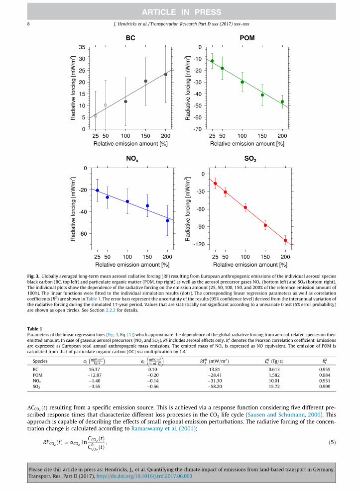
Fig. 3. Globally averaged long-term mean aerosol radiative forcing (RF) resulting from European anthropogenic emissions of the individual aerosol speciesblack carbon (BC, top left) and particulate organic matter (POM, top right) as well as the aerosol precursor gases NOx (bottom left) and SO2 (bottom right).The individual plots show the dependence of the radiative forcing on the emission amount (25, 50, 100, 150, and 200% of the reference emission amount of100%). The linear functions were fitted to the individual simulation results (dots). The corresponding linear regression parameters as well as correlationcoefficients (R2) are shown in Table 1. The error bars represent the uncertainty of the results (95% confidence level) derived from the interannual variation ofthe radiative forcing during the simulated 17-year period. Values that are statistically not significant according to a univariate t-test (5% error probability)are shown as open circles. See Section 2.2.2 for details.

Table 1Parameters of the linear regression lines (Fig. 3, Eq. (1)) which approximate the dependence of the global radiative forcing from aerosol-related species on theiremitted amount. In case of gaseous aerosol precursors (NOx and SO2), RF includes aerosol effects only. R2

i denotes the Pearson correlation coefficient. Emissionsare expressed as European total annual anthropogenic mass emissions. The emitted mass of NOx is expressed as NO equivalent. The emission of POM iscalculated from that of particulate organic carbon (OC) via multiplication by 1.4.

Species aimW=m2

Tg=a

� �ai

mW=m2

% of E0i

� �RF0i mW=m2

� �E0i Tg=að Þ R2

i

BC 16.37 0.10 13.81 0.613 0.955POM �12.87 �0.20 �28.41 1.582 0.984NOx �1.40 �0.14 �31.30 10.01 0.931SO2 �3.55 �0.56 �58.20 15.72 0.999


DCCO2 ðtÞ resulting from a specific emission source. This is achieved via a response function considering five different pre-scribed response times that characterize different loss processes in the CO2 life cycle (Sausen and Schumann, 2000). Thisapproach is capable of describing the effects of small regional emission perturbations. The radiative forcing of the concen-tration change is calculated according to Ramaswamy et al. (2001):

PleaseTransp

RFCO2 ðtÞ ¼ aCO2 lnCCO2 ðtÞC0CO2

ðtÞ ; ð5Þ

cite this article in press as: Hendricks, J., et al. Quantifying the climate impact of emissions from land-based transport in Germany.ort. Res. Part D (2017), http://dx.doi.org/10.1016/j.trd.2017.06.003



where C0CO2

ðtÞ is the background concentration as a function of time, CCO2 ðtÞ ¼ C0CO2

ðtÞ þ DCCO2 ðtÞ is the concentration per-turbed by the additional emissions considered, and aCO2 is a constant factor of 5.35 W/m2. In the present study, the back-

ground concentrations C0CO2

ðtÞ of the past were chosen according to measurements, whereas future projections weretaken from the RCP scenarios. We refer to Meinshausen et al. (2011) for a detailed description of these concentration profiles.

AirClim also derives changes in the mean concentration of methane from transport-induced modifications of the methanelifetime. To enable a consistent quantification of transport effects on ozone and methane, we take into account the methanelifetime change derived from the QCTM simulations as described in Section 2.2.1. The radiative forcing of the methane per-turbation is then calculated according to Ramaswamy et al. (2001) as a function of the concentration change and the back-ground concentration. As in the case of CO2, past and future background concentrations were chosen according toMeinshausen et al. (2011). Since the oxidation cycle of methane influences the ozone production, changes in the methaneconcentration lead to a further modification of the ozone concentration and a corresponding radiative forcing. This effectis considered according to Dahlmann et al. (2016). In the discussion of the AirClim results in Section 3.2 we have includedthis additional effect into the radiative forcing of methane since it is closely coupled to the direct methane effect and showsthe same timescales of the induced climate modifications.

2.2.4. Synthesis of atmospheric model resultsThe approaches described above enable the calculation of the radiative forcings resulting from changes in CO2, methane,

aerosol particles (direct and indirect effects), and ozone caused by regional transport emission sources. Beyond radiative forc-ing, the change in global mean surface temperature DT is a common metric for assessing global climate change. As alreadyindicated in Fig. 1, the responsemodel AirClim allows to deriveDT from the radiative forcings. Depending on the specific ques-tion addressed, alternative metrics can be derived from radiative forcing or DT. For a discussion of the most commonmetrics,their respective merits, and their applications, we refer to Fuglestvedt et al. (2010) and Grewe and Dahlmann (2015).

The temperature change resulting from RFCO2 ðtÞ is calculated with AirClim following the approach of Sausen andSchumann (2000), which applies a temperature response function based on simulations with a detailed globalatmosphere-ocean climate model (Cubasch et al., 1992). This function can also be applied to the radiative forcing of otherspecies. However, this requires that the resulting temperature responses are multiplied by the so-called efficacy parameter(Hansen et al., 2005), which accounts for the different sensitivities of temperature change to the radiative forcings inducedby perturbations of different atmospheric species. We assume efficacy parameters of 1.37 and 1.18 for ozone and methane,respectively (Ponater et al., 2006). For aerosol-induced climate effects we use an efficacy parameter of 1. This is a conserva-tive choice reflecting that existing estimates of the parameter for aerosols depend strongly on the applied model and on thetype of the emissions as well as their spatial distribution (Hansen et al., 2005; Shine et al., 2012). Aerosol efficacy is one of thelargest unknowns in this research area.

For assessing the climate effects of the different species, their atmospheric residence times need to be considered in orderto account for the long-term accumulation of long-lived species in the atmosphere and the resulting increased climaticimpact of these compounds. Simulations of time periods of the order of centuries are necessary to achieve this for CO2.To evaluate the effects of transport-induced emissions in our application example, we considered the time period from1850 to 2100. Hence, the AirClim simulations range from the time when the growth of land-based transport volumes began,to future years which are described by widely-used scenarios of future emissions (i.e., the RCPs).

As explained in Section 2.2.1, the transport-induced ozone radiative forcing as well as the change in methane lifetimewere calculated with the detailed chemistry model EMAC for a selected time slice (2030) only. To simulate the effects inother years, we assume that the ozone radiative forcing and the methane lifetime modification change proportionally tothe NOx emissions (Section 3.1) since NOx is the major driver of these effects. As outlined above, the radiative forcing of aero-sol perturbations can be calculated as the sum of the contributions of different aerosol constituents. If the emissions of theindividual aerosol species and aerosol precursors are known as a function of time, the linear relations described above can beapplied to the respective time period. Particularly for the past, such emission data is lacking. However, information aboutpast emissions of total particulate matter is available (Section 3.1). Hence, we assume that the past aerosol-induced climateeffects are proportional to the total particulate matter emissions.

The radiative forcings of the transport-induced CO2 and methane perturbations depend on the background concentra-tions of these species. To account for the uncertainty of the respective future background concentrations in our demonstra-tion application, we performed AirClim simulations considering three different future scenarios: RCP2.6, RCP4.5, and RCP8.5,which cover a wide range of possible background conditions, from comparatively low (RCP2.6) over medium (RCP4.5) to veryhigh (RCP8.5) concentrations (Meinshausen et al., 2011). The results of these simulations are time series of radiative forcingand changes in global mean surface temperature obtained individually for each of the different radiatively active species(CO2, aerosol, ozone, methane).

2.3. Transport and emission modeling

2.3.1. Transport modelingAs a basis for the calculation of emissions from land-based transport within Germany for present-day conditions and dif-

ferent future scenarios, a transport modeling approach was developed within the VEU project to assess transport demand




and the resulting transport activity (Fig. 2). The aim of these transport modeling efforts was to provide all relevant informa-tion for emission modeling on an aggregated German level, that is, for calculating German total emissions from ground-based transport. In view of these goals, the modeling approach was derived to meet the following requirements:

1. All relevant land-based transport activities have to be covered. This includes both passenger and freight transport byall land-based transport modes (road, rail, and inland navigation).

2. Structural changes, like demographic trends, with relevance for transport demand and consequently transport emis-sions have to be represented. Furthermore, the applied models have to be sensitive to other demand influencing fac-tors, such as costs, varying between the scenarios considered.

3. Despite the aggregation of the German emissions, the approach should be capable of considering also measuresapplied on smaller scales, for instance, local measures implemented only in specific cities. This implies that the spa-tial resolution of the applied models should be high enough to represent such measures.

4. For flexibility reasons, the chosen approach should be generic enough to be applicable to areas different from the cur-rent analysis area (Germany).

In the modeling methodology followed here, transport demand is modeled on macroscopic level, which means that indi-viduals eliciting similar travel behavior are aggregated to groups. The calculations are based on socio-economic data (forinstance, information about economic development, population, households, workforce, income levels) and provideorigin-destination-matrices for several thousand traffic analysis zones (TAZs). The surrounding countries are aggregatedto additional traffic zones. The description of demand distinguishes between vehicle, train, and vessel types on road, rail,and inland waterways, respectively, in case of freight transport and between the modes motorized private transport, publictransport, bicycles, and pedestrians for passenger transport (Table 2). To generate all information required for emission mod-eling, the modes of motorized transport are further split into different vehicle technology categories, according to powertrainand fuel type (such as diesel, gasoline, or electrified) and emission classes (Euro standards). For passenger cars, the shares ofthe different vehicle technologies are explicitly modeled to reflect changes in the energy mix as well as the penetration ofnew technologies like electrified vehicles and vehicles complying with more stringent emission standards. Based on theorigin-destination-matrices, demand is assigned to the traffic network by quantifying link flows (number of vehicle move-ments per time period between network nodes) to describe the transport activity.

The combination of models for passenger transport, freight transport, and vehicle technologies makes the approach ver-satile and compliant with the requirements described above. Interdependencies between demand and traffic, between vehi-cle technologies and demand, and between freight and passenger traffic can be taken into account. The individual modelingapproaches, as applied for the assessment of the baseline scenario considered here, are described in the following.

In order to model passenger travel demand, the EVA model (Vrtic et al., 2007) is adopted. EVA is a disaggregated macro-scopic model of personal travel behavior and traffic flow. As a first step, EVA defines the number of produced and attractedtrips for each travel zone, based on spatially disaggregated empirical data, like population and workforce information. Thenumber of trips is calculated for different trip purposes like work or education. Subsequently, destination and mode choiceare calculated simultaneously. The final result are the all-traffic flows for any combination of origin, destination, and mode.

To describe travel demand for Germany appropriately, the country is divided into 6561 traffic analysis zones, which rep-resent origins and destinations of the trips. The purpose-specific traffic volume is calculated for each zone. For this reason,many different input data sets are required. In particular, detailed information about population (e.g., age, sex, income, carownership) and its temporal development is of high relevance. This information is taken from different external data sources(e.g., BBSR, 2009). As mentioned above, not only motorized private transport and public transport but also cycling and walk-ing are considered. Taking into account non-motorized modes for a nationwide model is due to the requirement to representall relevant mode shifts on land, as shifts to and from these modes result in emission changes.

The macroscopic freight transport model (Müller et al., 2012) is based on information about the German economy (forinstance, gross-value added of distinct economic activities or number of employees in these sectors), which is taken from

Table 2Means of transport considered in the applied transport models. The abbreviation ‘gw’ stands for thevehicles’ gross weight.

Transport type Transport means

Passenger transport Motorized private transport, public transport, cycling, walking

Freight transportInland waterways: Small barges, large barges, tankersRailway: Trainload, wagonload, combined transportRoad: Light duty vehicles (gw 6 3.5 t),

Heavy duty vehicles 1 (3.5 t < gw 6 7.5 t),Heavy duty vehicles 2 (7.5 t < gw 6 12 t),Heavy duty vehicles 3 (gw > 12 t, without tractor-trailer combinations)Heavy duty vehicles 4 (gw > 12 t, tractor-trailer combinations)




an external forecast (IWH, 2006). The correlation of economic indicators with the amount of goods transported is used toderive the freight generation (attraction and production of freight transport). Thus changes in the economic structure leadto changes in the modeled freight transport demand. The spatial distribution of freight flows is described by a gravity modelapproach which takes the freight generated in the traffic zones as attraction/production and derives the deterrence measurefrom transport cost and travel times between these zones. The assignment to one of three ground-based transport modes(road, rail, ship) follows random utility-based discrete choice theory. The conversion of freight flows to vehicle trips usestransport statistics in order to determine vehicle class-dependent gross weight, load factors, and empty trip rates.

After calculating the origin-destination-matrices for all modes, these trips need to be assigned to the traffic network(roads, railways, waterways) in order to derive level-of-service data for destination and mode choice as well as to calculatethe route choice. The relevant network of all land-based modes is represented by over one million links and 470.000 nodes.As a result, the trip assignment generates detailed information about the traffic volume of the assigned modes on each link.An exception is public transport which is described in terms of aggregated traffic volumes, as we do not have all data nec-essary to assign trips to the network (e.g., lines, line routes, time profiles).

In addition to modeling the traffic volumes, knowledge on vehicle technologies and their evolution over time is essentialto calculate emissions. For the VEU application, we used the agent-based vehicle technology scenario model VECTOR21(Mock, 2010) for simulating the competition between conventional and alternative powertrains for the new passenger carmarket in Germany. In the applied version, 900 types of customers are modeled using costs of ownership as a basis for theirpurchase decision, taking into account the political framework for CO2 emission targets. In addition, the passenger car fleet ismodeled including energy consumption and CO2 emissions. The fleet composition is assessed by applying a stock modelingapproach. Starting from the initial year, fleet turnover is modeled taking into account the vehicle age distribution and sur-vival rates to describe the diffusion of innovative technologies into the stock. The results were used, together with the trans-port volumes on the road network, as a basis for describing the emissions.

2.3.2. Emission modelingTo calculate transport emissions, transport activities (in terms of mileages) are multiplied by corresponding emission fac-

tors, which describe the amount of specific pollutants released by specific vehicles per distance travelled. To calculate Ger-man transport emissions for 2008, 2020, and 2030, we applied the activity data for motorized private transport, busses, lightand heavy duty vehicles, passenger and freight rail transport, and inland navigation (Section 2.3.1). Due to differences in thevehicle-specific emission factors, we used the road transport activity data divided into the different categories according toengine capacity, European emission standard (EURO 0–6), and fuel type (gasoline, diesel, liquefied petroleum gas (LPG), com-pressed natural gas (CNG), and electricity). For rail transport we applied activity data divided into electric and diesel traction.To complement the activity data, activities for off-road transport (e.g., in construction or agriculture) were taken from theresults of TIMES PanEU energy system model runs (Blesl et al., 2008). The emission factors for road transport including coldstarts and gasoline evaporation were chosen according to HBEFA (2010). An exception were black and organic carbon (BC,OC) particulate matter emissions which were calculated with emission factors described by Samaras (2013). For rail trans-port we applied emission factors reported by EMEP/EEA (2012).

The quantification of transport-induced ozone changes (Section 2.2.1) requires short-lived species emission data also forGerman non-transport sectors and for all sectors in other European countries. For 2008 these data were chosen according toCLRTAP (2011). Emission data for 2020 and 2030 were also calculated on the basis of activity data and corresponding emis-sion factors. Future activity data for the different sectors were estimated by means of energy demand modeling with theTIMES PanEU model mentioned above. For the transport sector, the final energy consumptions (i.e., energy used by the finalconsumer) for road transport, rail transport, and navigation were modeled separately. For each of the transport modes, themodel considers a variety of conventional and alternative fuels (e.g., biofuels, methanol, natural gas, LPG, dimethyl ether(DME), hydrogen, electricity). In order to complement the baseline scenario of German transport emissions by a baselineestimate of the European emissions up to 2030, our assumptions for the future energy consumption in the EU27 were basedon current European legislation and targets, with 2010 as reference year. The following key assumptions were made:

1. Reduction of the greenhouse gas emissions in the EU and Germany by 20% and 30%, respectively, until 2020, and 30%and 40%, respectively, until 2030 compared to 1990.

2. Reduction of EU-wide greenhouse gas emissions from the sectors included in the ETS (Emission Trading System) by21% until 2020 compared to 2005.

3. Increasing minimum production of electricity from renewables: 30% in the EU by 2030 and 30% in Germany by 2020.4. Market shares for hybrid electric, battery electric, and plug-in hybrid electric vehicles of less than 10% each.5. Implementation of EU directive 2009/28/EC requesting a minimum quota of 10% renewable fuels in transport final

energy consumption by 2020.6. Share of biofuels in Germany: 7% in all years.

We refer to Blesl et al. (2010) and Bruchof and Voß (2010) for further energy modeling details. The emission factors tocalculate the emissions for 2020 and 2030 for all source categories except for the transport sector were chosen in analogyto the GAINS model approach (Amann et al., 2008). For the transport sector in Europe (except Germany), emission factorswere adopted from the transport emission database of the TREMOVE 3.5 model (TML, 2011). Corresponding emissions of




the aerosol components OC and BC were calculated from the total amount of suspended particles according to Kupiainen andKlimont (2004).

3. Results and discussion

3.1. Transport and emissions

As an exemplary result of the transport models described in Section 2.3.1, Fig. 4 shows the aggregated German annualmileage of different road vehicle types in 2008, 2020 and 2030. The mileage of passenger cars is by far the highest of allmeans of transport and is projected to increase by 8%, from 600 to 649 billion kilometers, between 2008 and 2030. Althoughwe assume that the population in Germany declines in the future, an expected increase in average distance travelled causesthis considerable increase of driven mileage. The mileages of freight transport by the different road-based means of transportincrease as well and show larger growth rates than the passenger car segment. For instance, the mileage of heavy duty vehi-cles increases by over 60% between 2008 and 2030. It is important to note that the resulting emission shares of the differentvehicle types (see below) may deviate strongly from corresponding mileage shares due to large differences in fuel consump-tion and emission factors. It should also be noted that the results are based on data from before the economic crisis startingin 2007. Thus they do not exactly reflect recent developments, which could lead to different growth rates. The data, however,are sufficient to demonstrate the applicability of our methods.

The corresponding transport-induced emissions calculated with the methods described in Section 2.3.2 are shown inFig. 5, in terms of total annual emissions of the different species. We show both German and corresponding European trans-port emissions as total amount and relative contributions to the total anthropogenic emissions in the respective area, againfor the years 2008, 2020, and 2030. In the following we refer to these emission data as the ‘VEU emissions’. An additionalanalysis of the various emission contributions (not shown) reveals that the calculated transport emissions are dominatedby road transportation. Contributions of railways and inland navigation are relevant only for a few species considered,but even in these cases they only contribute a few percent to the respective total transport emissions. The results shownin Fig. 5 reveal that transport is a major source of NOx and CO in Germany. The contributions to total German anthropogenicemissions of these two species amount to 31% and 34% in 2008, respectively. The emission calculations also provide infor-mation about the contributions of specific vehicle types to the respective emissions (not shown). In 2008, the transport-induced NOx emissions in Germany are mainly caused by heavy duty vehicles (55% of total transport NOx emissions, dom-inated by emissions of tractor-trailer combinations) and passenger cars (34%). Transport-induced CO emissions stem from alarger variety of sources (55% from passenger cars, 20% frommopeds and motorcycles, 12% from light duty vehicles, and 11%from heavy duty vehicles). Transport also makes a large contribution to the anthropogenic emissions of CO2 in Germany (22%in 2008). This is mainly due to emissions from passenger cars (75% of total transport CO2 emissions) and heavy duty vehicles(18%). Transport emissions also significantly contribute to the German total anthropogenic emissions of black carbon (16% in2008), non-methane VOC (14%), and particulate organic carbon (12%). Note, that for application in the atmospheric aerosolsimulations, the emitted amount of particulate organic carbon (OC) is transformed to emissions of particulate organic matter(POM) via multiplication by a factor of 1.4 (Righi et al., 2013).

The results obtained for German transport further suggest that a strong decrease in the emissions of short-lived specieswill occur in the near future, owing to advances in vehicle technology. For instance, electrified vehicles reach a share of 40%of the passenger car fleet in the VECTOR21 simulations for 2030, with 13% of the fleet being pure battery (non-hybrid) elec-tric vehicles. This results from assuming stringent CO2 emission targets for new passenger cars in combination with anexpansion of charging infrastructure, moderate electricity prices, and targeted tax reductions, in order to reach the nationalgoal of one million electrified vehicles until 2020. The emission reduction until 2030 is smaller but still significant in case ofCO2 since the effects of reductions in the vehicle specific emissions are partly offset by increasing transport volumes. As a

Fig. 4. Transport activity in Germany as calculated with the applied transport models. The figure shows annual mileages for passenger cars (blue), lightduty vehicles (red), and heavy duty vehicles (dark grey) in the years 2008, 2020, and 2030.



Fig. 5. Annual emissions of land-based transport in Germany (red bars) and Europe (blue bars) calculated within the VEU project (see text for more details).The figure shows emissions of nitrogen oxides (NOx, expressed as NO equivalent), carbon monoxide (CO), non-methane volatile organic compounds(NMVOC, labelled as VOC in the plots), ammonia (NH3), particulate black and organic carbon (BC, OC), sulfur dioxide (SO2) and carbon dioxide (CO2).Absolute emission amounts (left) as well as the relative contribution to total anthropogenic emissions (right) in the years 2008 (top), 2020 (middle), and2030 (bottom) are presented. The total amounts of the respective emissions are given at the bottom of each bar. Absolute emissions are given in Tg for CO2

and Gg for all other species. Note the logarithmic scaling of the absolute emissions.


consequence, the relative contributions of transport emissions decrease in the case of short-lived species but stay nearly onthe same level as in 2008 in case of CO2. The emissions calculated for Europe-wide transport show similar characteristics asthose of the German transport system. However, the emissions of most short-lived species show larger relative contributionsto total emissions than in Germany, especially in 2008. This can be explained by the higher average age of the vehicle fleet ofmany European countries. Another important difference is that the calculated European transport CO2 emissions increase inthe future, which can be attributed to a slower efficiency improvement of conventional vehicles as well as a less stringentimplementation of alternative fuels and powertrains. For instance, according to our assumptions (Section 2.3.2), the pene-tration of electric vehicles into the market occurs more slowly on the European level than in Germany. The calculated emis-sions generally show large differences in the individual amounts of the different species released. However, it should benoted that the mere amount cannot be taken as proxy for the climate impact when comparing the effects of the individualspecies since they show very different efficiencies for inducing climate change (e.g., Myhre et al., 2013). Hence, a detailedquantification of the individual climatic impacts, as carried out in the present study, is inevitable.

For some species, the transport-induced emissions calculated here are larger than the corresponding values reported bythe German federal environment agency (UBA) which are part of the emission inventories published by the UNFCCC (UnitedNations Framework Convention on Climate Change). For instance, the CO2 emissions of German transport in 2008 amount to218 Tg according to our calculations while UBA reports a value of 153 Tg only. These discrepancies result from conceptualdifferences in the methodical approaches. For instance, according to the Kyoto protocol, national emissions reported in theUNFCCC data base have to be calculated on the basis of the amount of fuel sold in the respective country. In contrast, thevalues obtained here result from bottom-up calculations including also movements of vehicles fueled in neighboring coun-tries, for instance, as a reaction to higher German fuel prices. This includes transit freight transport as well as passengertransport and explains an important fraction of the additional transport emissions derived in the present study.

Since the VEU emission data are confined to the time period between 2008 and 2030, additional data sets had to be con-sidered and assumptions had to be made in order to yield German transport emissions for the whole time period from 1850to 2100 (Section 2.2.4). For the years 1990–2008, we used the emission inventories of transport-induced CO2, NOx, and totalparticulate matter reported annually by UBA. We scaled these data to match the corresponding VEU emissions in 2008 in




order to compensate for discrepancies due to methodological differences. For 1970–1990, we used data on CO2 emissionsfrom European transport which were generated within the EU project QUANTIFY (Borken-Kleefeld et al., 2010; Uhereket al., 2010). Since spatially resolved emission data from that project are only available for 2000, we used the 1970–1990EU15 total transport emissions. To estimate the German contribution, we rescaled the EU15 totals according to the relativecontribution of Germany to the EU15 emissions in 2000. The obtained data were scaled to match the 1990 values of the1990–2008 data generated as described above, to compensate for methodological differences in emission assessment. Theresulting values were then linearly extrapolated back to 1950. To estimate emissions for earlier years, we assumed a linearincrease of the German transport-induced CO2 emissions from zero in 1850 to the 1950 value calculated as described above.Since land-based transport emissions were negligibly small in the first half of the 19th century, the choice of 1850 as startingpoint as well as the assumption of zero emissions in this year are both justified.

The resulting time series of CO2 emissions is presented in Fig. 7a. The major features of these past emissions are a com-paratively small increase until about 1950 followed by a rapid growth until the last decade of the 20th century. This behavioris very similar to that of the global anthropogenic CO2 emissions reported, for instance, by Meinshausen et al. (2011). For thefuture years 2030–2100 we conservatively assumed that transport-induced CO2 emissions remain constant at the 2030 level,since we refrain from projections without robust model-based calculations.

For specifying transport-induced NOx emissions throughout the period 1850–2100, we followed a similar strategy as forCO2. VEU data were used for 2008–2030 and constant values at the 2030 level are assumed until 2100. As mentioned above,values for the past were taken from the UBA database back to 1990, and scaled to match the VEU data in 2008. Emissionsprior to 1990 were assumed to change in proportion to CO2 emissions. This approach was also chosen to calculate particleemissions. Since consistent information about past emissions of the individual aerosol species black and organic carbon isnot available, we considered total particulate matter emissions and derived the past values of the total aerosol-inducedRF from the value calculated for 2008 by assuming that the aerosol RF changes in proportion to the total particulate matteremission. Transport emissions of SO2, an important precursor of sulfate aerosol, were not taken into account since they arenegligible for the VEU years, due to the very low sulfur content of present-day fuels. Also ammonia (NH3) from transport isneglected because of the very small amount emitted. It should be noted that rough assumptions on past emissions of short-lived species can be regarded as less critical since long-term accumulation effects are negligible.

3.2. Climate effects

As a first step to quantify the atmospheric impact of the transport emissions, the EMAC model in the QCTM configurationwas applied as described in Section 2.2.1. For these simulations, we employed the European emission inventory for the year2030 (Sections 2.3.2) generated in the VEU project and embedded in the RCP8.5 global emission data set for the same year.To quantify the transport-induced effects, we compared a simulation, in which European transport emissions are neglected,to a reference simulation including the full set of emissions. The differences of these two model runs (‘reference run’ minus‘simulation with reduced emissions’) can be interpreted as the transport-induced signal. Recall that, in the QCTM application,we quantified the effects of the European transport emissions to enhance the signal-to-noise ratio. The results were thenscaled down to the effects of the German transport system.

Fig. 6 shows concentrations of NOx, ozone (O3), and the hydroxyl radical (OH) as a function of altitude (and equivalent airpressure) and latitude. The concentrations were averaged over the three simulated years and the respective circle of latitude.The figure presents background concentrations not including contributions from European transport (left column) as well asthe corresponding absolute (middle column) and relative (right column) transport-induced changes. Note that the effects ofthe transport emissions show pronounced longitudinal variations (not displayed), especially at lower altitudes where par-ticularly large perturbations occur over Europe and its surroundings.

The results clearly indicate that in areas with increased transport-induced NOx also the ozone and OH concentrationsincrease. The changes mainly occur in the northern hemisphere, with largest effects at those latitudes where the emissionsare released. Compared to the respective background concentrations in these areas, the concentrations of NOx, ozone, and OHincrease by up to 4%, 0.5%, and 1%, respectively. Such small perturbations were to be expected since European transport con-tributes only a few percent to the global anthropogenic NOx emissions. In addition, large fractions of the background con-centrations result from natural sources, such as NOx emissions from lightning or ozone intrusions from the stratosphere.The magnitude of the transport-induced effects demonstrates that we have to deal with comparably small perturbations thatwould be hard to detect within a fully-coupled chemistry-climate model simulation, particularly in the case of O3 and OH. Inthe QCTM simulation, the perturbations show only very small interannual variations, which implies that the dependence ofthe chemical effects on the specific meteorological characteristics of the different years is small and, consequently, the quan-tified signals can be regarded as highly significant.

Since ozone is a greenhouse gas, an increase in its concentration results in a positive radiative forcing, which correspondsto a warming of the atmosphere. The global radiative forcing due to the ozone perturbation induced by European transportemissions in 2030 as derived from the QCTM simulations amounts to 1.29 mW/m2. According to Section 2.2.1, this value wasscaled down to obtain a forcing of the German transport emissions of 0.072 mW/m2 in 2030. The corresponding relativechanges of the methane lifetime, induced by the increase in OH, amount to �0.0838% and, if downscaled, �0.0047%. Thereduction in methane lifetime implies a decrease in the methane concentration and a resulting cooling effect, which partlyoffsets the ozone-induced warming (see below). As mentioned in Section 2.2.1, the contribution of transport emissions to



Fig. 6. Global simulation of trace gas concentrations and their transport-induced changes. Shown are annual mean zonal average concentrations of NOx (toprow), ozone (O3) (middle row), and OH (bottom row) simulated considering emissions of the year 2030. The results are plotted as a function of geographicallatitude and altitude (or equivalent air pressure). The figure presents background concentrations obtained by neglecting European transport emissions (leftcolumn), their absolute change due to European transport emissions (middle column), and corresponding relative changes (right column). Note thedifferent units used for background concentrations and transport-induced changes. 1E-n stands for 10�n . The largest changes occur in the troposphere(lowest part of the atmosphere; the white line indicates the tropopause, which marks the boundary between the troposphere and the stratosphere above).


atmospheric ozone can be underestimated by the perturbation method by factors of up to 5. We will consider this uncer-tainty in the discussion of the role of ozone-related climate impacts below.

The aerosol radiative forcing resulting from the German transport emissions of particles (BC and OC) and particle precur-sors (mainly NOx) described in Section 3.1 was calculated according to Eq. (4). These calculations result in transport-inducedaerosol radiative forcings of �0.62, �0.27, and �0.18 mW/m2 in 2008, 2020, and 2030, respectively. Hence, the aerosol effectcalculated for 2030 is of similar magnitude as the corresponding ozone effect, but of opposite sign. The transport-inducedaerosol has a cooling effect, which counteracts the ozone-induced warming. According to Section 2.2.4, the aerosol and ozoneradiative forcing values in combination with the methane lifetime change due to German transport emissions were used asinput for the AirClim simulations, which were performed as the last step to obtain an overall assessment of the climateimpact. In addition, the information about the emissions of CO2, NOx, and total aerosol during the whole analyzed periodfrom 1850 to 2100 (Section 3.1) was used to calculate the CO2 effect and to describe the temporal developments.




The assumed long-term development of the German transport emissions as well as the resulting radiative forcing of thedifferent species and corresponding change of the global mean surface temperature simulated with AirClim are displayed inFig. 7. Results for selected years are also presented in Table 3. Due to its very long residence time and the resulting accumu-lation in the atmosphere over time, CO2 causes the largest radiative forcing among the considered species. The forcing exhi-bits a strong increase, particularly between 1950 and 2000. Under assumption of background concentrations according tothe RCP8.5 scenario, the maximum forcing of 14.4 mW/m2 is reached around 2025. Due to the long-term accumulation, atime shift of about 25 years occurs between the maximum emissions around the year 2000 and this maximum radiative forc-ing. Values of around 14 mW/m2 are persistent during the first decades of the 21st century. These values are of the order of1% of the total anthropogenic CO2 forcing, which amounted to about 1.7 W/m2 in 2011 (Myhre et al., 2013), for instance.

Unfortunately, an evaluation of this result by comparison with observational data is not possible, since global perturba-tions of CO2 and the resulting changes of the Earth’s radiation budget cannot be simply attributed to very specific emissionsources, such as German road transport, through measurements. However, the plausibility of the results can be evaluated forthe year 2000 since climatic impacts of global transport emissions have been analyzed for this year in previous studies. TheAirClim simulations suggest that the radiative forcing induced by the CO2 emissions of the German transport systemamounts to about 12 mW/m2 in 2000. By simply scaling this number with the ratio of the global to the national number

Fig. 7. Temporal change of (a) the transport-induced emissions of CO2, NOx (expressed as NO equivalent, multiplied by 100), and particulate matter(primary aerosol, i.e., BC and POM, multiplied by 1000) assumed for Germany between 1850 and 2100 as well as (b) the resulting radiative forcings (RF) and(c) changes in global mean surface temperature (DT) simulated with AirClim. The vertical lines indicate the years covered by the VEU emission data set. Thedifferent solutions for future radiative forcing and temperature change due to CO2 result from different assumptions on future CO2 backgroundconcentrations according to different future scenarios (RCP2.6, RCP4.5, and RCP8.5). Effects of CH4 differ only slightly among the scenarios. Hence, O3 + CH4

values are shown for RCP8.5 only. The blue shaded area denotes the uncertainty ranging from O3 + CH4 to 5�O3 + CH4. For values obtained for selected yearsin the different AirClim simulations, we refer to Table 3. Note that aerosol effects resulting from SO2 emissions are not considered. See text for more detailson this simplification.



Table 3Radiative forcing RF [mW/m2] and change of global mean surface temperature DT [mK] due to changes in CO2, ozone, methane, and aerosol induced by Germantransport emissions. In addition the sum of ozone and methane effects (as highlighted in Fig. 7) is shown. The values are extracted from the AirClim simulationsfor selected years. In case of the long-lived greenhouse gases CO2 and CH4, results of simulations for different scenarios (RCPs 2.6, 4.5, and 8.5) are presented.The values given for CH4 include also the effects of long-term ozone modifications resulting from transport-induced methane changes. Values for the timebefore 1950 are not shown since they are only small. Up to the year 2000 the simulations are identical since the future scenarios start in that year. Ozone andaerosol effects do not vary among the scenarios (see text for more details on this assumption). The uncertainty range limit 5�O3 + CH4 is shown for RCP8.5 only,due to the similarity of the scenarios.

Species Scenario 1950 1990 2000 2008 2020 2030 2100

Transport-induced RF [mW/m2]CO2 RCP8.5 2.50 9.24 11.98 13.39 14.32 14.29 9.64

RCP4.5 2.50 9.24 11.98 13.39 14.48 14.74 16.75RCP2.6 2.50 9.24 11.98 13.39 14.45 14.89 21.41

O3 All 0.09 0.63 0.49 0.28 0.13 0.07 0.07

CH4 RCP8.5 �0.05 �0.30 �0.33 �0.29 �0.19 �0.12 �0.07RCP4.5 �0.05 �0.30 �0.33 �0.29 �0.19 �0.12 �0.05RCP2.6 �0.05 �0.30 �0.33 �0.30 �0.20 �0.12 �0.05

O3+CH4 RCP8.5 0.04 0.33 0.16 �0.01 �0.06 �0.05 0.00RCP4.5 0.04 0.33 0.16 �0.01 �0.06 �0.05 0.02RCP2.6 0.04 0.33 0.16 �0.02 �0.07 �0.05 0.02

5�O3+CH4 RCP8.5 0.40 2.85 2.12 1.11 0.46 0.23 0.28

Aerosol All �0.23 �1.53 �1.15 �0.62 �0.27 �0.18 �0.18

Transport-induced DT [mK]CO2 RCP8.5 1.00 3.13 4.24 5.22 6.58 7.47 8.05

RCP4.5 1.00 3.13 4.24 5.22 6.59 7.54 10.74RCP2.6 1.00 3.13 4.24 5.22 6.59 7.55 12.72

O3 All 0.06 0.28 0.34 0.34 0.30 0.25 0.10

CH4 RCP8.5 �0.02 �0.11 �0.15 �0.18 �0.18 �0.17 �0.08RCP4.5 �0.02 �0.11 �0.15 �0.18 �0.18 �0.17 �0.07RCP2.6 �0.02 �0.11 �0.15 �0.18 �0.19 �0.17 �0.07

O3 + CH4 RCP8.5 0.04 0.17 0.19 0.16 0.12 0.08 0.02RCP4.5 0.04 0.17 0.19 0.16 0.12 0.08 0.03RCP2.6 0.04 0.17 0.19 0.16 0.11 0.08 0.03

5�O3 + CH4 RCP8.5 0.28 1.29 1.55 1.52 1.32 1.08 0.42

Aerosol All �0.11 �0.50 �0.61 �0.60 �0.52 �0.43 �0.18


of road vehicles in 2000 (about 7:5 � 108 versus 4:5 � 107) a forcing of 200 mW/m2 is obtained which is in the order of theforcing of global road and rail transport CO2 emissions of 175(±21) mW/m2 reported by Uherek et al. (2010) based on resultsof Fuglestvedt et al. (2008). It should be noted that scaling the rail contribution with the number of road vehicles is probablyuncritical due to the small contribution of rail emissions. Scaling the 12 mW/m2 with land-based transport-induced CO2

emissions in 2000 results in a very similar global transport effect (assuming global emissions of 4400 Tg according toUherek et al. (2010) versus national emissions of 260 Tg according to Section 3.1). We would like to stress that these esti-mates are just approximations since the CO2 effect depends also on the history of the transport activities, that is, the pastdevelopment of the global-versus-national-ratio of the numbers of vehicles or CO2 emissions, respectively. Nevertheless,the estimates indicate that the obtained magnitude of the simulated forcing is plausible.

The AirClim results presented in Fig. 7 further reveal that the long-term future development of the CO2-related radiativeforcing of the German transport emissions strongly depends on the chosen background scenario (Section 2.2.4). Using dif-ferent scenarios enables us to estimate the uncertainty due to assumptions about future global emissions by spanning a pos-sible range of future developments. After 2030 the forcing further increases to values around 21 mW/m2 in 2100 if theRCP2.6 background scenario is assumed. In this case the CO2 background concentrations decrease. This results in an increas-ing German transport effect due to the nonlinear dependence of the CO2 radiative forcing on its atmospheric burden (thesmaller the CO2 background concentration, the larger the radiative forcing of additional CO2 released into the atmosphere;Eq. (5)). In contrast, the forcing is decreasing to values around 10 mW/m2 when RCP8.5 is assumed where the backgroundconcentration shows a huge future increase and the climate effect per emitted amount of CO2 is declining. RCP4.5 also showsan increase in the background concentration which weakens during the 21st century and stops in 2100. This results in a forc-ing in between those of the two other scenarios.

The modeled increase in global mean surface temperature DT induced by the CO2 emissions of German transport behavessimilar to the corresponding radiative forcing. However, the essential difference is that DT reacts much more slowly tochanges of the emissions. Time shifts of more than a decade occur between corresponding features in RF and DT. This ismainly due to the long time scales of the ocean temperature to adjust to the atmospheric changes. As a consequence, DT




shows a gradual increase in RCPs 2.6 and 4.5 without plateau, as occurring in the radiative forcing development, and a lesspronounced decrease in the late 21st century in RCP8.5. The future temperature change is of the order of 10 mK and rangesbetween 8.1 mK (RCP8.5) and 12.7 mK (RCP2.6) in 2100. In the year 2000, DT amounts to 4.2 mK. In analogy to the radiativeforcing, this value can be scaled up to the effect of global land-based transport. This results in an estimated temperaturechange of about 70 mK which is consistent with the value of 80 mK reported by Uherek et al. (2010) based on results ofSkeie et al. (2009).

Our simulations suggest that aerosol particles from German transport emissions induce noticeable effects only betweenabout 1950 and 2020 (RF) and 1970 and 2050 (DT). The negative values imply that aerosols induce a cooling and thereforepartly counteract the warming effect of CO2. The aerosol-induced DT is largest around the year 2000 amounting to �0.6 mK,which offsets 14% of the CO2 effect. Due to reductions in the emissions of aerosol particles and aerosol precursor gases (hereNOx), the aerosol effects decline in the future and are very small compared to the CO2 effect at the end of the 21st century.The aerosol effects were not quantified for different background scenarios since they show an approximately linear behaviorfor a wide range of concentrations as discussed in Section 2.2.2.

It is important to stress that the quantification of the aerosol impact suffers from large uncertainties. Many aerosol-related processes, such as aerosol effects on ice clouds, the formation of secondary organic aerosol from volatile organic com-pounds, or the effects of non-exhaust vehicle emissions (tire and break wear, resuspension of road dust) which mightincrease in the future due to increasing traffic volume, are still poorly understood and were therefore not considered inthe present calculations. Taking into account such processes could lead to different estimates of the aerosol-induced climateeffects.

The modeled RF and DT resulting from the transport-induced ozone and methane modifications are even smaller than thecorresponding aerosol effects. However, we need to consider that the ozone effect is probably underestimated by the per-turbation method. In an extreme case, about 5 times more ozone could be produced which would result in an ozone effectexceeding the aerosol impact. It is common to analyze the sum of the warming ozone and cooling methane effects since theyare initiated by the same emission components. The net effect is a warming during the whole simulated period with a max-imum DT between 0.2 and 1.6 mK around the year 2000, taking into account the uncertainty range of the ozone perturbation.Hence, the simulations reveal that, compared to the dominant CO2-induced warming, this additional warming effect couldhave been of considerable importance during that time. Due to the declining emissions and its non-cumulative (and there-fore episodic) character, this additional warming decreases to rather small values in our future projection.

The ozone and methane effects exhibit interesting features which might become very relevant if our approach would beapplied to scenarios for countries with higher non-CO2 emissions resulting from less stringent emission regulations. Forinstance, the simulations show that the net radiative forcing related to ozone and methane becomes negative over a few dec-ades in the first half of the 21st century (Table 3, O3 + CH4). This is due to the ozone-related radiative forcing decreasing fas-ter than the corresponding methane-induced forcing, which is a consequence of the longer response time of the methaneconcentration to emission changes. The net effect turns to positive values again when the emissions stay constant. Theresults also suggest that, in contrast to CO2, transport-induced methane causes very similar temperature changes in the dif-ferent scenarios. This is due to a smaller variability of the methane background among the scenarios as well as due to a com-pensation of two effects controlling the climate impact of the methane perturbation. On the one hand, the transport-inducedmethane reduction increases with increasing background concentration since the reduction in methane lifetime applies tototal methane. On the other hand, the radiative forcing of the methane perturbation decreases with increasing backgroundconcentration, due to similar nonlinearities as discussed for CO2.

In this context, it should be noted that due to the huge computational expenses of the QCTM simulations the transport-induced ozone production and CH4 lifetime reduction have been quantified for RCP8.5 only, while the CH4 background con-centrations in the AirClim simulations are varied according to the underlying RCP scenarios. This discrepancy appears to beuncritical in the present application since the methane effects are of secondary importance. However, if the methods devel-oped here would be applied to regions where emissions of short-lived species, inducing the CH4 perturbations, are more rel-evant, QCTM simulations for different background scenarios would be necessary.

It is of vital importance to stress that the conclusions drawn from our assessment of the climate effects of German trans-port emissions do not hold for global transport. While non-CO2 effects are less important in our simulations they are muchmore relevant if global transport effects are in focus (Righi et al., 2013, 2015). This can be attributed to higher non-CO2-to-CO2 transport emission ratios in many other areas of the globe, such as Southeast Asia. In addition, emissions of short-livedspecies released in other geographical areas could have larger climatic impacts per emitted amount. Even though the sim-ulated effects of German transport emissions of non-CO2 species are comparably small, it is important to note that the fea-sibility of the new approach to quantify such small effects could be demonstrated. This modeling capability is a majorprerequisite to evaluate mitigation strategies applied to regional transport systems only. The method is ready for operationaluse and can be applied also to transport systems of other regions.

4. Conclusions

We have developed a method to quantify the global climate effects of regional transport emissions. This new approachovercomes the methodological difficulties to detect the effects of regional emissions of short-lived species with conventional




global three-dimensional chemistry-climate simulations. These difficulties arise from the large natural variability of the cli-mate system and the resulting poor signal-to-noise ratios for small perturbations. The new method is based on a combina-tion of simulations performed with a comprehensive global chemistry-climate model and a climate response model. It iscomplemented by a set of aerosol-climate response functions. The approach enables the quantification of the effects of allrelevant emission components including particulate matter, short-lived gaseous pollutants, and long-lived greenhouse gases.To demonstrate its applicability, the method was applied to results from a transport and emission model suite which allowsthe description of the current and scenario-based future German transport activities and the related emissions. This enabled,for the first time, to quantify and compare the individual climatic impacts of the different species emitted by the Germantransport system.

Simulations performed for a baseline scenario of German transport activities suggest that German transport emissionsinduce an increase of the global mean surface temperature of the order of 10 mK during the 21st century. The model calcu-lations further suggest that this climate impact is dominated by the emissions of CO2. The magnitude of the temperaturechange depends on the assumptions for the CO2 background concentration, which is controlled by the future developmentof global anthropogenic emissions.

The dominance of the climate effect of CO2 over the non-CO2 effects is different from the corresponding impact of globaltransport emissions, where non-CO2 species make a larger relative contribution to transport-induced climate change than inthe case of German transport emissions. This is mainly due to larger emission shares and possibly also larger climate impactsper emitted mass of non-CO2 species released in other areas of the globe. The comparatively small climate effects of non-CO2

species from German transport emissions does not imply that these emissions are generally irrelevant. For instance, legalthresholds for particulate matter concentrations are frequently exceeded in major German cities, with large contributionsfrom transport emissions. In this context, it is also important to stress that the quantification of non-CO2 climate effects suf-fers from uncertainties due to still existing gaps in understanding the roles of a number of specific atmospheric processesinvolved, particularly related to the effects of aerosol particles. This implies that future studies might result in significantmodifications of the modeled climatic impacts of non-CO2 species.

Our new climate modeling approach in combination with the applied transport and emission models offers the possibilityto generate different future transport scenarios for Germany and to assess the corresponding climate effects. In principle, ourclimate modeling approach can also be applied to other regions, including areas where non-CO2 emissions are more impor-tant than in the case of Germany, for instance, Asian countries. This would require an extension of the set of aerosol-climateresponse functions by descriptions of the aerosol impact for these regions, based on simulations with a detailed three-dimensional aerosol-climate model. In addition, new QCTM simulations focusing on gas-phase effects of emissions releasedin the respective areas would be necessary.

The following further improvements could help to reduce the uncertainties and to enhance the efficiency and flexibility ofour method. The quantification of the contributions of transport emissions to atmospheric ozone with the applied QCTMmodel suffers from nonlinearities in the dependence of the ozone production rate on the amount of NOx emissions. To reducethe related uncertainties, tagging methods to track the transport contribution directly in the simulation of the chemical sys-tem could be applied (Grewe et al., 2012). Tagging transport-induced OH may also help to advance the quantifications of themethane lifetime modifications resulting from transport emissions. Since three-dimensional chemistry-climate models asthe QCTM used here are computationally expensive and therefore not suitable to assess a large number of scenarios, a cli-mate response model to quantify transport effects on ozone and methane lifetime directly from the emissions is desirable.The development of such a model is an ongoing activity in the VEU project. To improve the simulations of transport-inducedaerosol effects, the applied models should be extended to include processes which have been neglected so far, such as aerosoleffects on ice clouds, the formation and climate impacts of secondary organic aerosols, or the emission and effects of non-exhaust particles from tire and brake abrasion or resuspension of road dust.

In addition, large progress would be made by the development of a climate response model covering the effects of all rel-evant emission components. This could be achieved by combining the existing climate response model AirClim with theaerosol-climate response functions and the response model currently developed to quantify ozone and methane changes.Such an overall approach would allow for efficient and self-consistent assessments of the climate impacts even for a largenumber of transport scenarios and would facilitate Monte-Carlo-like simulations with varying input parameters to analyzesensitivities and uncertainties (as in Dahlmann et al., 2016, for aviation emissions). A test bed for this approach could be theassessment of scenarios for the development of the German transport system up to 2040 which are currently elaboratedwithin VEU.

The response functions applied in climate response models allow the quantification of climate effects directly from theemissions, even in case of very small emission perturbations. Hence, these models enable not only the assessment of climateeffects for scenarios describing the entire transport system. They also allow the analysis of the potential benefits resultingfrom specific measures to mitigate transport-induced climate change. For instance, political measures like incentives or reg-ulations to establish sustainable vehicle technologies or measures fostering a modal shift in passenger and freight transportcould be the focus. Also very specific measures, such as the implementation of new exhaust treatment systems, could beassessed, and the benefits of different measures could be compared.




Acknowledgements

This study has been conducted in the framework of the institutionally funded project ‘Transport and the Environment(VEU)’ of the German Aerospace Center (DLR). The EMAC simulations were performed at the German Climate ComputingCenter (DKRZ, Hamburg, Germany). We wish to thank Axel Lauer for fruitful discussions and valuable comments on themanuscript. We also thank two anonymous reviewers for their well-founded comments which helped to further increasethe scientific and technical quality of the article.

References

Amann, M., Bertok, I., Cofala, J., Heyes, C., Klimont, Z., Rafaj, P., Schöpp, W., Wagner, F., 2008. National Emission Ceilings for 2020 based on the 2008 Climate& Energy Package. NEC Scenario Analysis Report Nr. 6. International Institute for Applied Systems Analysis (IIASA), Laxenburg, Austria. <www.iiasa.ac.at/rains/reports/NEC6-final110708.pdf>.

BBSR, Federal Institute for Research on Building, Urban Affairs and Spatial Development, 2009. Raumordnungsprognose 2025/2050, Berichte, Band 29, Bonn,Germany. ISBN 978-3-87994-079-0.

Berntsen, T.K., Fuglestvedt, J.S., Joshi, M.M., Shine, K.P., Stuber, N., Ponater, M., Sausen, R., Hauglustaine, D.A., Li, L., 2005. Response of climate to regionalemissions of ozone precursors: sensitivities and warming potentials. Tellus 57B, 283–304.

Berntsen, T., Fuglestvedt, J., Myhre, G., Stordal, F., Berglen, T.F., 2006. Abatement of greenhouse gases: does location matter? Clim. Change 74, 377–411.Blesl, M., Kober, T., Bruchof, D., Kuder, R., 2008. Beitrag von technologischen und strukturellen Veränderungen im Energiesystem der EU-27 zur Erreichung

ambitionierter Klimaschutzziele. ZfE Zeitschrift für Energiewirtschaft 4, 219–229.Blesl, M., Kober, T., Bruchof, D., Kuder, R., 2010. Effects of climate and energy policy related measures and targets on the future structure of the European

energy system in 2020 and beyond. Energy Policy 38, 6278–6292.Borken-Kleefeld, J., Berntsen, T., Fuglestvedt, J., 2010. Specific climate impact of passenger and freight transport. Environ. Sci. Tech. 44, 5700–5706.Bruchof, D., Voß, A., 2010. Analysis of the Potential Contribution of Alternative Fuels and Power Trains to the Achievement of Climate Targets in the EU27.

Full Paper. International Energy Workshop (IEW), Stockholm 2010.Chow, J.C. et al, 2006. Health effects of fine particulate air pollution: lines that connect. J. Air Waste Manage. Assoc. 56, 1368–1380.CLRTAP, 2011. Emission Data Officially Submitted by the Parties to the Convention on Long Range Transboundary Air Pollution to the EMEP Programme.Cubasch, U., Hasselmann, K., Höck, H., Maier-Reimer, E., Mikolajewicz, U., Santer, B.D., Sausen, R., 1992. Time-dependent greenhouse warming computations

with a coupled ocean-atmosphere model. Clim. Dyn. 8, 55–69.Dahlmann, K., Grewe, V., Ponater, M., Matthes, S., 2011. Quantifying the contributions of individual NOx sources to the trend in ozone radiative forcing.

Atmos. Environ. 45, 2860–2868.Dahlmann, K., Grewe, V., Frömming, C., Burkhardt, U., 2016. Can we reliably assess climate mitigation options for air traffic scenarios despite large

uncertainties in atmospheric processes? Transp. Res. Part D Transp. Environ. 46, 40–55.Deckert, R., Jöckel, P., Grewe, V., Gottschaldt, K.-D., Hoor, P., 2011. A quasi chemistry-transport model mode for EMAC. Geosci. Model Dev. 4, 195–206.EMEP/EEA Air Pollutant Emission Inventory Guidebook 2009 (update 2012), 2012. Technical Report No 6/2009. European Environment Agency,

Kopenhagen.Eyring, V. et al, 2010. Transport impacts on atmosphere and climate: shipping. Atmos. Environ. 44, 4735–4771.Frömming, C., Ponater, M., Dahlmann, K., Grewe, V., Lee, D.S., Sausen, R., 2012. Aviation-induced radiative forcing and surface temperature change in

dependency of the emission altitude. J. Geophys. Res. 117, D19104.Fuglestvedt, J.S., Berntsen, T., Myhre, G., Rypdal, K., Skeie, R.B., 2008. Climate forcing from the transport sectors. Proc. Natl. Acad. Sci. USA 105, 454–458.Fuglestvedt, J.S., Shine, K.P., Berntsen, T., Cook, J., Lee, D.S., Stenke, A., Skeie, R.B., Velders, G.J.M., Waitz, I.A., 2010. Transport impacts on atmosphere and

climate: metrics. Atmos. Environ. 44, 4648–4677.German Federal Ministry for the Environment, Nature Conservation, Building and Nuclear Safety, 2007. Report on Implementation of the Key Elements of an

Integrated Energy and Climate Programme Adopted in the Closed Meeting of the Cabinet on 23/24 August 2007 in Meseberg, Germany. <www.bmub.bund.de/N40589-1/>.

Gottschaldt, K., Voigt, C., Jöckel, P., Righi, M., Deckert, R., Dietmüller, S., 2013. Global sensitivity of aviation NOx effects to the HNO3-forming channel of theHO2 + NO reaction. Atmos. Chem. Phys. 13, 3003–3025.

Grewe, V., Dahlmann, K., 2012. Evaluating climate-chemistry response and mitigation options with AirClim. In: Schumann, U. (Ed.), Atmospheric Physics.Background – Methods – Trends. Springer, Berlin, Heidelberg, Germany, pp. 591–606.

Grewe, V., Dahlmann, K., 2015. How ambiguous are climate metrics? And are we prepared to assess and compare the climate impact of new air traffictechnologies? Atmos. Environ. 106, 373–374.

Grewe, V., Stenke, A., 2008. AirClim: an efficient tool for climate evaluation of aircraft technology. Atmos. Chem. Phys. 8, 4621–4639.Grewe, V., Dahlmann, K., Matthes, S., Steinbrecht, W., 2012. Attributing ozone to NOx emissions: implications for climate mitigation measures. Atmos.

Environ. 59, 102–107.Grewe, V., Champougny, T., Matthes, S., Frömming, C., Brinkop, S., Søvde, O.A., Irvine, E.A., Halscheidt, L., 2014. Reduction of the air traffic’s contribution to

climate change: a REACT4C case study. Atmos. Environ. 94, 616–625.Hansen, J. et al, 2005. Efficacy of climate forcings. J. Geophys. Res. 110, D18104.HBEFA, 2010. The Handbook Emission Factors for Road Transport, Version 3.1. <http://www.hbefa.net>.Hoor, P. et al, 2009. The impact of traffic emissions on atmospheric ozone and OH: results from QUANTIFY. Atmos. Chem. Phys. 9, 3113–3136.IWH, Halle Institute for Economic Research, 2006. Regionalisierte Wirtschafts- und Außenhandelsprognose für die Verkehrsprognose 2025.Jöckel, P. et al, 2006. The atmospheric chemistry general circulation model ECHAM5/MESSy1: consistent simulation of ozone from the surface to the

mesosphere. Atmos. Chem. Phys. 6, 5067–5104.Joshi, M., Shine, K., Ponater, M., Stuber, N., Sausen, R., Li, L., 2003. A comparison of climate response to different radiative forcings in three general circulation

models: towards an improved metric of climate change. Climate Dyn. 20, 843–854.Kahn Ribeiro, S. et al, 2007. Transport and its infrastructure. In: Metz, B., Davidson, O.R., Bosch, P.R., Dave, R., Meyer, L.A. (Eds.), Climate Change 2007:

Mitigation. Contribution of Working Group III to the Fourth Assessment Report of the Intergovernmental Panel on Climate Change. CambridgeUniversity Press, Cambridge, United Kingdom and New York, NY, USA.

Koffi, B., Szopa, S., Cozic, A., Hauglustaine, D., van Velthoven, P., 2010. Present and future impact of aircraft, road traffic and shipping emissions on globaltropospheric ozone. Atmos. Chem. Phys. 10, 11681–11705.

Kupiainen, K., Klimont Z., 2004. Primary Emissions of Submicron and Carbonaceous Particles in Europe and the Potential for their Control. Report IR-04-079.International Institute for Applied Systems Analysis, IIASA, Laxenburg, Austria.

Lauer, A., Eyring, V., Hendricks, J., Jöckel, P., Lohmann, U., 2007. Global model simulations of the impact of ocean-going ships on aerosols, clouds, and theradiation budget. Atmos. Chem. Phys. 7, 5061–5079.


http://www.iiasa.ac.at/rains/reports/NEC6-final110708.pdf

http://www.iiasa.ac.at/rains/reports/NEC6-final110708.pdf

http://refhub.elsevier.com/S1361-9209(16)30382-0/h0015























http://www.bmub.bund.de/N40589-1/

http://www.bmub.bund.de/N40589-1/


















http://www.hbefa.net















Lauer, A., Eyring, V., Corbett, J.J., Wang, C., Winebrake, J.J., 2010. Assessment of near-future policy instruments for oceangoing shipping: impact onatmospheric aerosol burdens and the Earths radiation budget. Environ. Sci. Tech. 43, 5592–5598.

Lee, D.S. et al, 2010. Transport impacts on atmosphere and climate: aviation. Atmos. Environ. 44, 4678–4734.Lund, M.T., Eyring, V., Fuglestvedt, J., Hendricks, J., Lauer, A., Lee, D., Righi, M., 2012. Global-mean temperature change from shipping toward 2050: improved

representation of the indirect aerosol effect in simple climate models. Environ. Sci. Tech. 46, 8868–8877.Meinshausen, M. et al, 2011. The RCP greenhouse gas concentrations and their extensions from 1765 to 2300. Clim. Change 109, 213–241.Mock, P., 2010. Entwicklung eines Szenariomodells zur Simulation der zukünftigen Marktanteile und CO2-Emissionen von Kraftfahrzeugen (VECTOR21)

(Dissertation). DLR-Institute for Vehicle Concepts, Stuttgart, Germany.Müller, S., Wolfermann, A., Huber, S., 2012. A nation-wide macroscopic freight traffic model. Procedia – Soc. Behav. Sci. 54, 221–230. 15th meeting of the

Euro Working Group on Transportation, 10–13 Sep. 2012, Cité Descartes, France.Myhre, G. et al, 2013. Anthropogenic and natural radiative forcing. In: Stocker, T.F. et al. (Eds.), Climate Change 2013: The Physical Science Basis.

Contribution of Working Group I to the Fifth Assessment Report of the Intergovernmental Panel on Climate Change. Cambridge University Press,Cambridge, United Kingdom and New York, NY, USA.

Peters, K., Stier, P., Quaas, J., Graßl, H., 2012. Aerosol indirect effects from shipping emissions: sensitivity studies with the global aerosol-climate modelECHAM-HAM. Atmos. Chem. Phys. 12, 5985–6007.

Peters, K., Stier, P., Quaas, J., Graßl, H., 2013. Corrigendum to Peters et al. (2012). Atmos. Chem. Phys. 13, 6429–6430.Ponater, M., Pechtl, S., Sausen, R., Schumann, U., Hüttig, G., 2006. Potential of the cryoplane technology to reduce aircraft climate impact: a state-of-the-art

assessment. Atmos. Environ. 40, 6928–6944.Pope III, C.A., Dockery, D.W., 2006. Health effects of fine particulate air pollution: lines that connect. J. Air Waste Manage. Assoc. 56, 709–742.Ramaswamy, V. et al, 2001. Radiative forcing of climate change. In: Joos, F., Srinivasan, J. (Eds.), Climate Change 2001: The Scientific Basis. Contribution of

Working Group I to the Third Assessment Report of the Intergovernmental Panel on Climate Change. Cambridge University Press, Cambridge, UnitedKingdom and New York, NY, USA.

Righi, M., Klinger, C., Eyring, V., Hendricks, J., Lauer, A., Petzold, A., 2011. Climate impact of biofuels in shipping: global model studies of the aerosol indirecteffect. Environ. Sci. Tech. 45, 3519–3525.

Righi, M., Hendricks, J., Sausen, R., 2013. The global impact of the transport sectors on atmospheric aerosol: simulations for year 2000 emissions. Atmos.Chem. Phys. 13, 9939–9970.

Righi, M., Hendricks, J., Sausen, R., 2015. The global impact of the transport sectors on atmospheric aerosol in 2030 – Part 1: land transport and shipping.Atmos. Chem. Phys. 15, 633–651.

Righi, M., Hendricks, J., Sausen, R., 2016. The global impact of the transport sectors on atmospheric aerosol in 2030 – Part 2: aviation. Atmos. Chem. Phys. 16,4481–4495.

Samaras, Z., 2013. Methodology for the Quantification of Road Transport PM-emissions, Using Emission Factors or Profiles. EU-FP7 Project TRANSPHORM,Deliverable D1.1.2 Report. <www.transphorm.eu>.

Sausen, R., 2010. Transport impacts on atmosphere and climate. Atmos. Environ. 44, 4646–4647.Sausen, R., Schumann, U., 2000. Estimates of the climate response to aircraft CO2 and NOx emissions scenarios. Clim. Change 44, 27–58.Sausen, R., Gierens, K., Eyring, V., Hendricks, J., Righi, M., 2012. Climate impact of transport. In: Schumann, U. (Ed.), Atmospheric Physics. Background –

Methods – Trends. Springer, Berlin, Heidelberg, Germany, pp. 711–725.Shindell, D., Schulz, M., Ming, Y., Takemura, T., Faluvegi, G., Ramaswamy, V., 2010. Spatial scales of climate response to inhomogeneous radiative forcing. J.

Geophys. Res. 115, D19110.Shine, K.P., Highwood, E.J., Rädel, G., Stuber, N., Balkanski, Y., 2012. Climate model calculations of the impact of aerosols from road transport and shipping.

Atmos. Oceanic Opt. 25, 62–70.Skeie, R.B., Fuglestvedt, J.S., Berntsen, T., Lund, M.T., Myhre, G., Rypdal, K., 2009. Global temperature change from the transport sectors: historical

development and future scenarios. Atmos. Environ. 43, 6260–6270.Stocker, T.F. et al, 2013. Technical Summary. In: Stocker, T.F. et al. (Eds.), Climate Change 2013: The Physical Science Basis. Contribution of Working Group I

to the Fifth Assessment Report of the Intergovernmental Panel on Climate Change. Cambridge University Press, Cambridge, United Kingdom and NewYork, NY, USA.

TML, 2011. TREMOVE – Economic Transport and Emissions Simulation Model, Developed by K.U.Leuven and Transport & Mobility Leuven. <www.tmleuven.be/methode/tremove>.

Uherek, E. et al, 2010. Transport impacts on atmosphere and climate: land transport. Atmos. Environ. 44, 4772–4816.van Vuuren, D.P. et al, 2011. The representative concentration pathways: an overview. Clim. Change 109, 5–31.Vrtic, M., Fröhlich, P., Schüssler, N., Axhausen, K.W., Lohse, D., Schiller, C., Teichert, H., 2007. Two-dimensionally constrained disaggregate trip generation,

distribution and mode choice model: theory and application for a Swiss national model. Transp. Res. Part A 41, 857–873.






























http://www.transphorm.eu
















http://www.tmleuven.be/methode/tremove

http://www.tmleuven.be/methode/tremove






Documents

Transportation Research Part D - DLR Portalelib.dlr.de/115799/1/Hendricks-etal-TRD-2017.pdf · Quantifying the climate impact of emissions from land-based transport in Germany Johannes