Embed Size (px)
Citation preview
Transportation Problem
1. Production costs at factories 𝐹1, 𝐹2,𝐹3 and 𝐹4 are Rs. 2, 3, 1 and 5 respectively. The
production capacities are 50, 70, 40 and 50 units respectively. Four stores 𝑆1, 𝑆2 ,𝑆3 and 𝑆4 have
requirements of 25, 35, 105 and 20 units respectively. Using transportation cost matrix find the
transportation plan that is optimal considering the production costs also.
Stores
Factory
𝑆1 𝑆2 𝑆3 𝑆4
𝐹1 2 4 6 11
𝐹2 10 8 7 5
𝐹3 13 3 9 12
𝐹4 4 6 8 3
Solution:
Stores
Factory
𝑆1 𝑆2 𝑆3 𝑆4 Supply
𝐹1 2+2 4+2 6+2 11+2 50
𝐹2 10+3 8+3 7+3 5+3 70
𝐹3 13+1 3+1 9+1 12+1 40
𝐹4 4+5 6+5 8+5 3+5 50
Demand 25 35 105 20
Total demand = 25 + 35 + 105 + 20 = 185
Total supply = 50 + 70 + 40 + 50 = 210
Total demand ≠ Total supply. Therefore the problem is unbalanced.
Since the total supply is more than the total demand add an extra column with zero entries and
demand as the difference between their sums to make the problem balanced one.
4 6 8 13 0 50
13 11 10 8 0 70
14 4 10 13 0 40
9 11 13 8 0 50
25 35 105 20 25
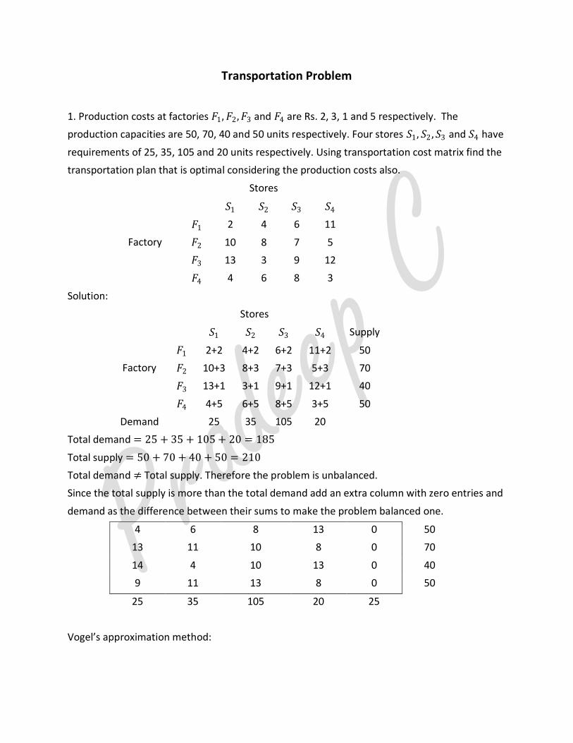
Vogel’s approximation method:
𝑀𝑖𝑛𝑖𝑚𝑢𝑚 𝑐𝑜𝑠𝑡 = 25 × 4 + 25 × 8 + 45 × 10 + 25 × 0 + 35 × 4 + 5 × 10 + 30 × 13
+20 × 8 = 1490
The number of basic cells = 8 = number of rows +number of columns – 1. Therefore the solution
is non degeneracy.
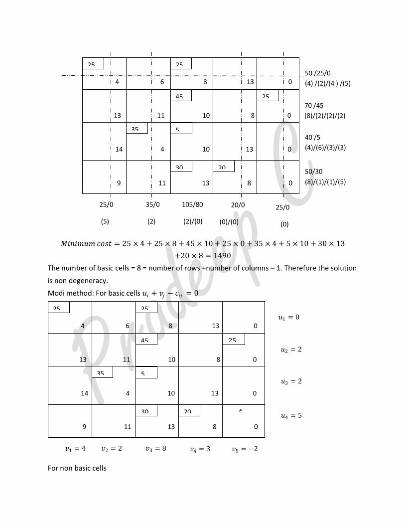
Modi method: For basic cells 𝑢𝑖 + 𝑣𝑗 − 𝑐𝑖𝑗 = 0
For non basic cells
4 6 8 13 0
13 11 10 8 0
14 4 10 13 0
𝜖
9 11 13 8 0
𝑣1 = 4
𝑢1 = 0
𝑣2 = 2 𝑣3 = 8 𝑣4 = 3 𝑣5 = −2
𝑢2 = 2
𝑢3 = 2
𝑢4 = 5
25
− 𝜖
35
25 25
20
45
5
30
4 6 8 13 0
13 11 10 8 0
14 4 10 13 0
9 11 13 8 0
25/0
(5)
50 /25/0
(4) /(2)/(4 ) /(5)
35/0
(2)
105/80
(2)/(0)
20/0
(0)/(0)
25/0
(0)
70 /45
(8)/(2)/(2)/(2)
40 /5
(4)/(6)/(3)/(3)
50/30
(8)/(1)/(1)/(5)
25
35
25 25
20
45
5
30
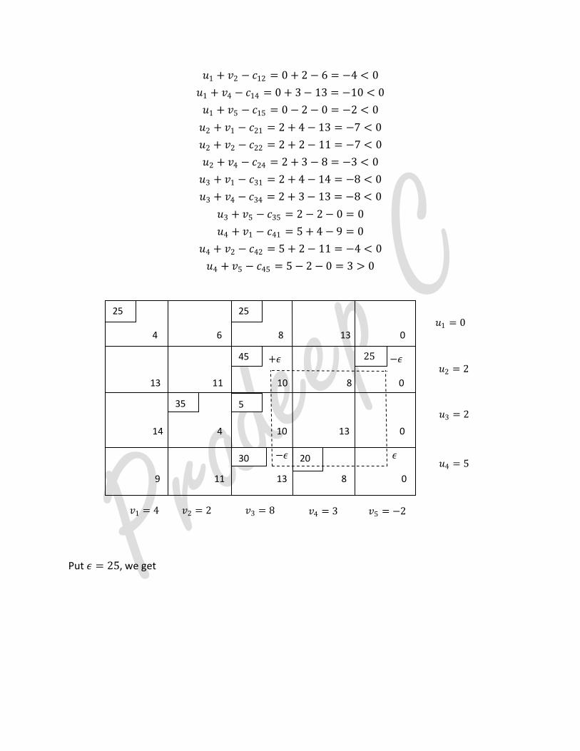
𝑢1 + 𝑣2 − 𝑐12 = 0 + 2 − 6 = −4 < 0
𝑢1 + 𝑣4 − 𝑐14 = 0 + 3 − 13 = −10 < 0
𝑢1 + 𝑣5 − 𝑐15 = 0 − 2 − 0 = −2 < 0
𝑢2 + 𝑣1 − 𝑐21 = 2 + 4 − 13 = −7 < 0
𝑢2 + 𝑣2 − 𝑐22 = 2 + 2 − 11 = −7 < 0
𝑢2 + 𝑣4 − 𝑐24 = 2 + 3 − 8 = −3 < 0
𝑢3 + 𝑣1 − 𝑐31 = 2 + 4 − 14 = −8 < 0
𝑢3 + 𝑣4 − 𝑐34 = 2 + 3 − 13 = −8 < 0
𝑢3 + 𝑣5 − 𝑐35 = 2 − 2 − 0 = 0
𝑢4 + 𝑣1 − 𝑐41 = 5 + 4 − 9 = 0
𝑢4 + 𝑣2 − 𝑐42 = 5 + 2 − 11 = −4 < 0
𝑢4 + 𝑣5 − 𝑐45 = 5 − 2 − 0 = 3 > 0
Put 𝜖 = 25, we get
4 6 8 13 0
+𝜖 −𝜖
13 11 10 8 0
14 4 10 13 0
−𝜖 𝜖
9 11 13 8 0
𝑣1 = 4
𝑢1 = 0
𝑣2 = 2 𝑣3 = 8 𝑣4 = 3 𝑣5 = −2
𝑢2 = 2
𝑢3 = 2
𝑢4 = 5
25
− 𝜖
35
25 25
20
45
5
30
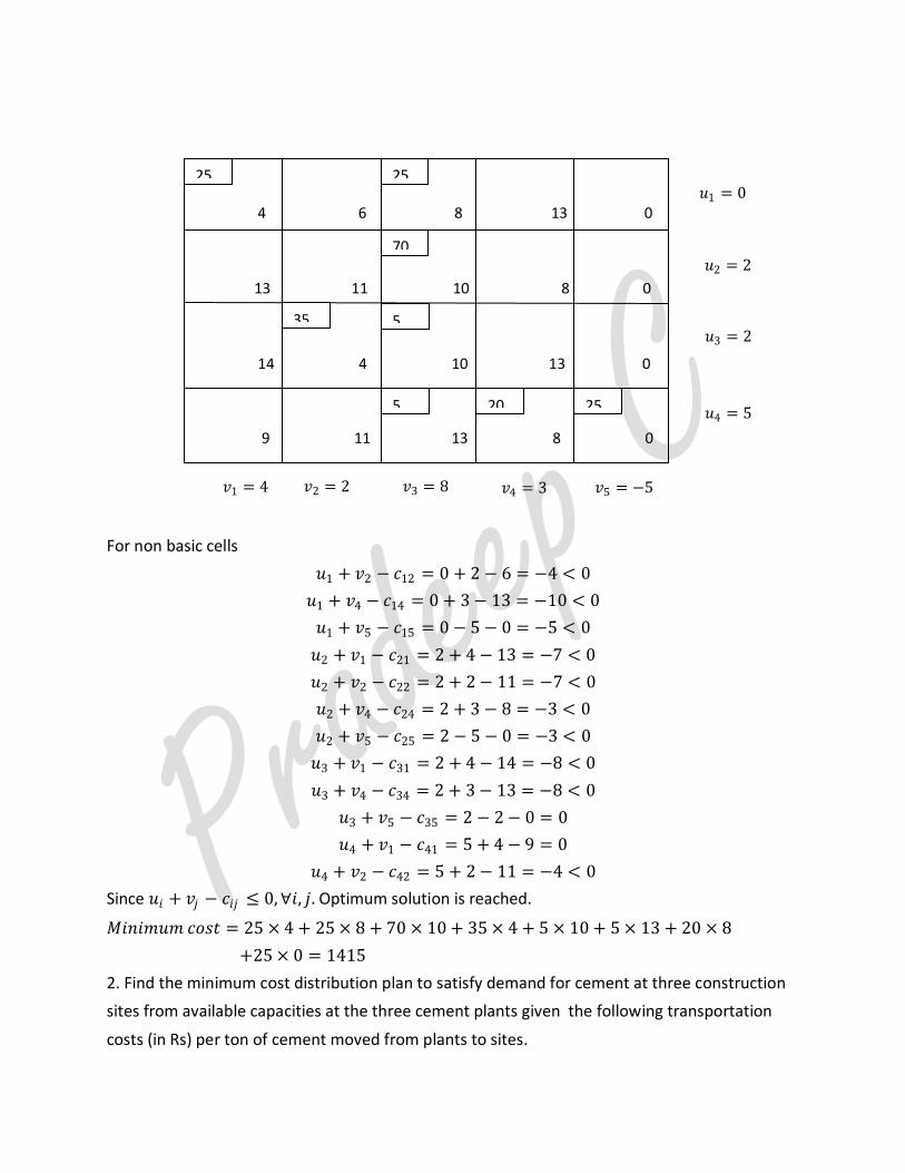
For non basic cells
𝑢1 + 𝑣2 − 𝑐12 = 0 + 2 − 6 = −4 < 0
𝑢1 + 𝑣4 − 𝑐14 = 0 + 3 − 13 = −10 < 0
𝑢1 + 𝑣5 − 𝑐15 = 0 − 5 − 0 = −5 < 0
𝑢2 + 𝑣1 − 𝑐21 = 2 + 4 − 13 = −7 < 0
𝑢2 + 𝑣2 − 𝑐22 = 2 + 2 − 11 = −7 < 0
𝑢2 + 𝑣4 − 𝑐24 = 2 + 3 − 8 = −3 < 0
𝑢2 + 𝑣5 − 𝑐25 = 2 − 5 − 0 = −3 < 0
𝑢3 + 𝑣1 − 𝑐31 = 2 + 4 − 14 = −8 < 0
𝑢3 + 𝑣4 − 𝑐34 = 2 + 3 − 13 = −8 < 0
𝑢3 + 𝑣5 − 𝑐35 = 2 − 2 − 0 = 0
𝑢4 + 𝑣1 − 𝑐41 = 5 + 4 − 9 = 0
𝑢4 + 𝑣2 − 𝑐42 = 5 + 2 − 11 = −4 < 0
Since 𝑢𝑖 + 𝑣𝑗 − 𝑐𝑖𝑗 ≤ 0,∀𝑖, 𝑗. Optimum solution is reached.
𝑀𝑖𝑛𝑖𝑚𝑢𝑚 𝑐𝑜𝑠𝑡 = 25 × 4 + 25 × 8 + 70 × 10 + 35 × 4 + 5 × 10 + 5 × 13 + 20 × 8
+25 × 0 = 1415
2. Find the minimum cost distribution plan to satisfy demand for cement at three construction
sites from available capacities at the three cement plants given the following transportation
costs (in Rs) per ton of cement moved from plants to sites.
4 6 8 13 0
13 11 10 8 0
14 4 10 13 0
𝜖
9 11 13 8 0
𝑣1 = 4
𝑢1 = 0
𝑣2 = 2 𝑣3 = 8 𝑣4 = 3 𝑣5 = −5
𝑢2 = 2
𝑢3 = 2
𝑢4 = 5
35
25 25
20
70
5
5 25
From Stores Capacity
(tons/month)
1 2 3
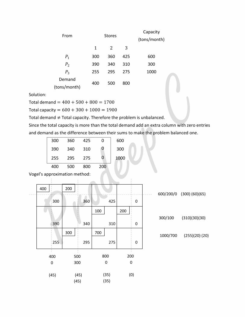
𝑃1 300 360 425 600
𝑃2 390 340 310 300
𝑃3 255 295 275 1000
Demand
(tons/month) 400 500 800
Solution:
Total demand = 400 + 500 + 800 = 1700
Total capacity = 600 + 300 + 1000 = 1900
Total demand ≠ Total capacity. Therefore the problem is unbalanced.
Since the total capacity is more than the total demand add an extra column with zero entries
and demand as the difference between their sums to make the problem balanced one.
300 360 425 0 600
390 340 310 0 300
255 295 275 0 1000
400 500 800 200
Vogel’s approximation method:
300 360 425 0
390 340 310 0
255 295 275 0
600/200/0 (300) (60)(65)
300/100 (310)(30)(30)
1000/700 (255)(20) (20)
400
0
(45)
500
300
(45)
(45)
200
300
800
0
(35)
(35)
200 400
100
200
0
(0)
700

𝑀𝑖𝑛𝑖𝑚𝑢𝑚 𝑐𝑜𝑠𝑡
= 400 × 300 + 200 × 360 + 100 × 310 + 200 × 0 + 300 × 295 + 700 × 275
= 504000
The number of basic cells = 6 = number of rows +number of columns – 1. Therefore the solution
is non degeneracy.
Modi method:
For basic cells 𝑢𝑖 + 𝑣𝑗 − 𝑐𝑖𝑗 = 0
For non basic cells
𝑢1 + 𝑣3 − 𝑐13 = 0 + 340 − 425 = −85 < 0
𝑢1 + 𝑣4 − 𝑐14 = 0 + 30 − 0 = 30 > 0
𝑢2 + 𝑣1 − 𝑐21 = −30 + 300 − 390 = −120 < 0
𝑢2 + 𝑣2 − 𝑐22 = −30 + 360 − 340 = −10 < 0
𝑢3 + 𝑣1 − 𝑐31 = −65 + 300 − 255 = −20 < 0
𝑢3 + 𝑣4 − 𝑐34 = −65 + 30 − 0 = −35 < 0
200 − 𝜖
300+𝜖
200 − 𝜖 400
100 + 𝜖
700 − 𝜖
300 360 425 0
390 340 310 0
255 295 275 0
𝑢1 = 0
200
300
200 400
100
700
𝑢2 = −30
𝑢3 = −65
𝑣1 = 300 𝑣4 = 30 𝑣3 = 340 𝑣2 = 360
𝜖
300 360 425 0
390 340 310 0
255 295 275 0
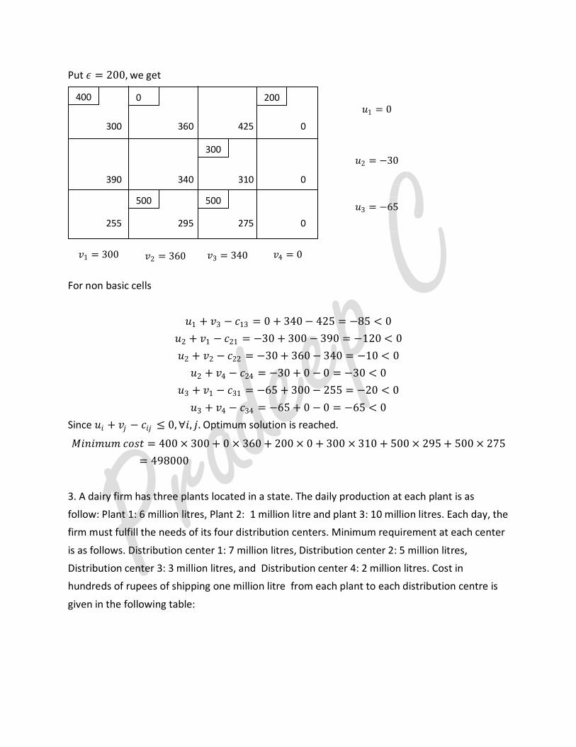
Put 𝜖 = 200, we get
For non basic cells
𝑢1 + 𝑣3 − 𝑐13 = 0 + 340 − 425 = −85 < 0
𝑢2 + 𝑣1 − 𝑐21 = −30 + 300 − 390 = −120 < 0
𝑢2 + 𝑣2 − 𝑐22 = −30 + 360 − 340 = −10 < 0
𝑢2 + 𝑣4 − 𝑐24 = −30 + 0 − 0 = −30 < 0
𝑢3 + 𝑣1 − 𝑐31 = −65 + 300 − 255 = −20 < 0
𝑢3 + 𝑣4 − 𝑐34 = −65 + 0 − 0 = −65 < 0
Since 𝑢𝑖 + 𝑣𝑗 − 𝑐𝑖𝑗 ≤ 0,∀𝑖, 𝑗. Optimum solution is reached.
𝑀𝑖𝑛𝑖𝑚𝑢𝑚 𝑐𝑜𝑠𝑡 = 400 × 300 + 0 × 360 + 200 × 0 + 300 × 310 + 500 × 295 + 500 × 275
= 498000
3. A dairy firm has three plants located in a state. The daily production at each plant is as
follow: Plant 1: 6 million litres, Plant 2: 1 million litre and plant 3: 10 million litres. Each day, the
firm must fulfill the needs of its four distribution centers. Minimum requirement at each center
is as follows. Distribution center 1: 7 million litres, Distribution center 2: 5 million litres,
Distribution center 3: 3 million litres, and Distribution center 4: 2 million litres. Cost in
hundreds of rupees of shipping one million litre from each plant to each distribution centre is
given in the following table:
300 360 425 0
390 340 310 0
255 295 275 0
𝑢1 = 0 200
500
0 400
300
500
𝑢2 = −30
𝑢3 = −65
𝑣1 = 300 𝑣4 = 0 𝑣3 = 340 𝑣2 = 360
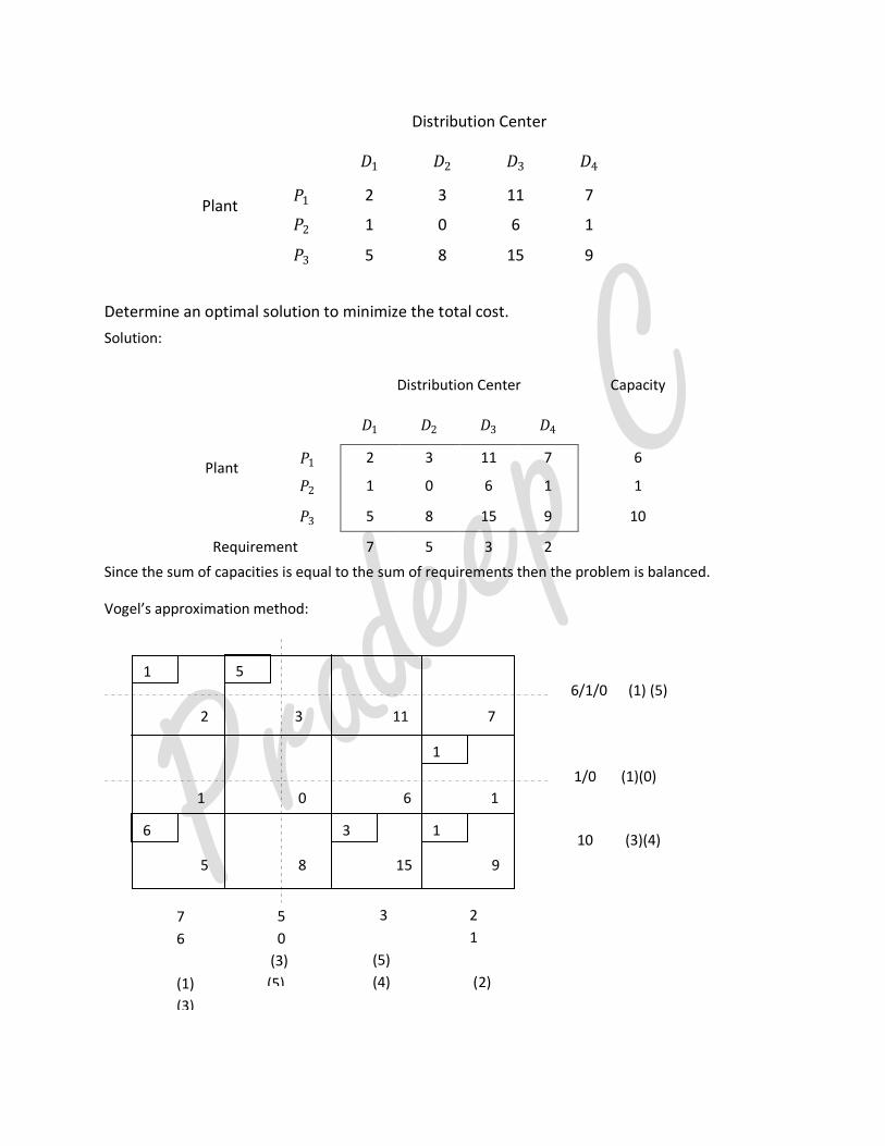
Distribution Center
Plant
𝐷1 𝐷2 𝐷3 𝐷4
𝑃1 2 3 11 7
𝑃2 1 0 6 1
𝑃3 5 8 15 9
Determine an optimal solution to minimize the total cost.
Solution:
Distribution Center Capacity
Plant
𝐷1 𝐷2 𝐷3 𝐷4
𝑃1 2 3 11 7 6
𝑃2 1 0 6 1 1
𝑃3 5 8 15 9 10
Requirement 7 5 3 2
Since the sum of capacities is equal to the sum of requirements then the problem is balanced.
Vogel’s approximation method:
2 3 11 7
1 0 6 1
5 8 15 9
6/1/0 (1) (5)
1/0 (1)(0)
10 (3)(4)
7
6
(1)
(3)
5
0
(3)
(5)
1
6
3
(5)
(4)
5 1
1
2
1
(2)
3
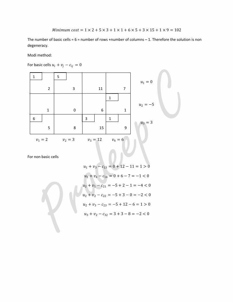
𝑀𝑖𝑛𝑖𝑚𝑢𝑚 𝑐𝑜𝑠𝑡 = 1 × 2 + 5 × 3 + 1 × 1 + 6 × 5 + 3 × 15 + 1 × 9 = 102
The number of basic cells = 6 = number of rows +number of columns – 1. Therefore the solution is non
degeneracy.
Modi method:
For basic cells 𝑢𝑖 + 𝑣𝑗 − 𝑐𝑖𝑗 = 0
For non basic cells
𝑢1 + 𝑣3 − 𝑐13 = 0 + 12 − 11 = 1 > 0
𝑢1 + 𝑣4 − 𝑐14 = 0 + 6 − 7 = −1 < 0
𝑢2 + 𝑣1 − 𝑐21 = −5 + 2 − 1 = −4 < 0
𝑢2 + 𝑣2 − 𝑐22 = −5 + 3 − 0 = −2 < 0
𝑢2 + 𝑣3 − 𝑐23 = −5 + 12 − 6 = 1 > 0
𝑢3 + 𝑣2 − 𝑐32 = 3 + 3 − 8 = −2 < 0
2 3 11 7
1 0 6 1
5 8 15 9
𝑢1 = 0
1
6
5 1
1 3
𝑢2 = −5
𝑢3 = 3
𝑣1 = 2 𝑣2 = 3 𝑣3 = 12 𝑣4 = 6
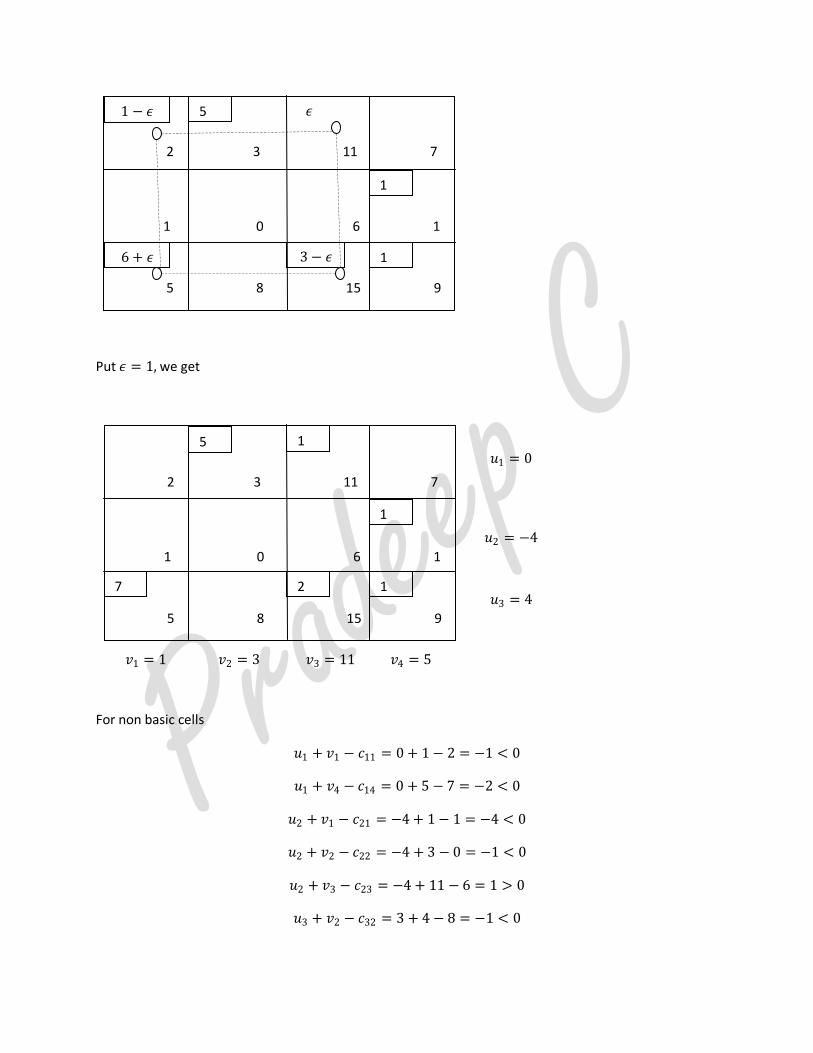
Put 𝜖 = 1, we get
For non basic cells
𝑢1 + 𝑣1 − 𝑐11 = 0 + 1 − 2 = −1 < 0
𝑢1 + 𝑣4 − 𝑐14 = 0 + 5 − 7 = −2 < 0
𝑢2 + 𝑣1 − 𝑐21 = −4 + 1 − 1 = −4 < 0
𝑢2 + 𝑣2 − 𝑐22 = −4 + 3 − 0 = −1 < 0
𝑢2 + 𝑣3 − 𝑐23 = −4 + 11 − 6 = 1 > 0
𝑢3 + 𝑣2 − 𝑐32 = 3 + 4 − 8 = −1 < 0
2 3 11 7
1 0 6 1
5 8 15 9
𝑢1 = 0
1
7
5 1
1 2
𝑢2 = −4
𝑢3 = 4
𝑣1 = 1 𝑣2 = 3 𝑣3 = 11 𝑣4 = 5
1
6 + 𝜖
5 1 − 𝜖
1 3 − 𝜖
𝜖
2 3 11 7
1 0 6 1
5 8 15 9
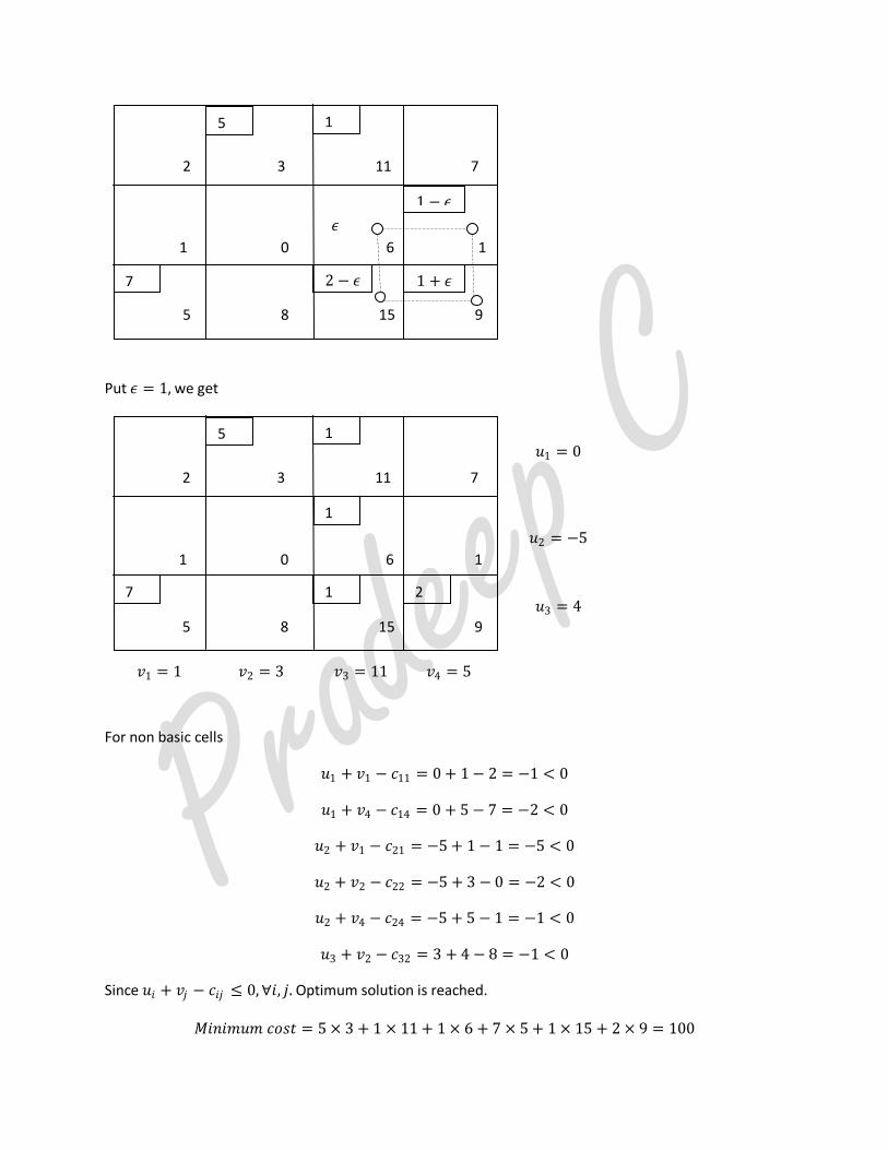
Put 𝜖 = 1, we get
For non basic cells
𝑢1 + 𝑣1 − 𝑐11 = 0 + 1 − 2 = −1 < 0
𝑢1 + 𝑣4 − 𝑐14 = 0 + 5 − 7 = −2 < 0
𝑢2 + 𝑣1 − 𝑐21 = −5 + 1 − 1 = −5 < 0
𝑢2 + 𝑣2 − 𝑐22 = −5 + 3 − 0 = −2 < 0
𝑢2 + 𝑣4 − 𝑐24 = −5 + 5 − 1 = −1 < 0
𝑢3 + 𝑣2 − 𝑐32 = 3 + 4 − 8 = −1 < 0
Since 𝑢𝑖 + 𝑣𝑗 − 𝑐𝑖𝑗 ≤ 0, ∀𝑖, 𝑗. Optimum solution is reached.
𝑀𝑖𝑛𝑖𝑚𝑢𝑚 𝑐𝑜𝑠𝑡 = 5 × 3 + 1 × 11 + 1 × 6 + 7 × 5 + 1 × 15 + 2 × 9 = 100
2 3 11 7
1 0 6 1
5 8 15 9
𝑢1 = 0
1
7
5 1
2 1
𝑢2 = −5
𝑢3 = 4
𝑣1 = 1 𝑣2 = 3 𝑣3 = 11 𝑣4 = 5
1 − 𝜖
7
5 1
1 + 𝜖
2 − 𝜖
2 3 11 7
𝜖
1 0 6 1
5 8 15 9
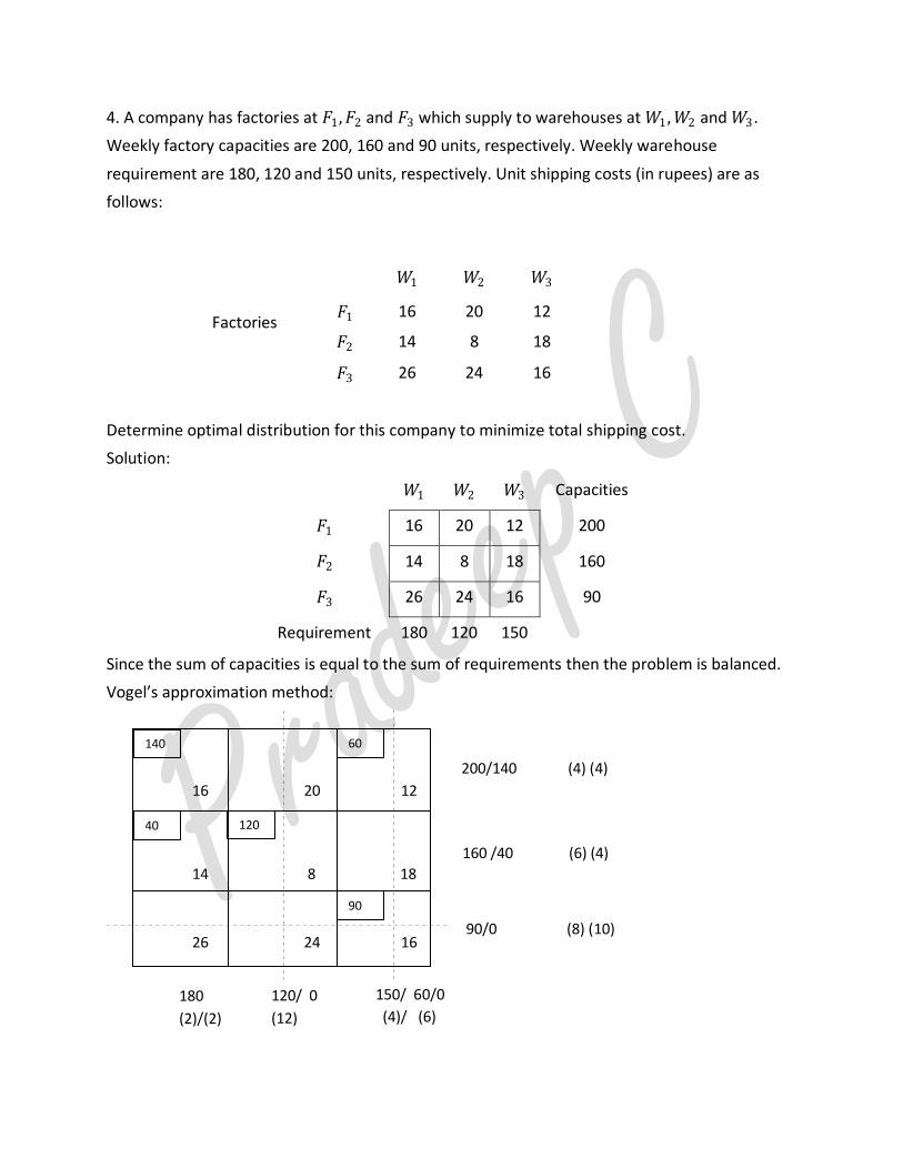
4. A company has factories at 𝐹1,𝐹2 and 𝐹3 which supply to warehouses at 𝑊1 , 𝑊2 and 𝑊3.
Weekly factory capacities are 200, 160 and 90 units, respectively. Weekly warehouse
requirement are 180, 120 and 150 units, respectively. Unit shipping costs (in rupees) are as
follows:
Factories
𝑊1 𝑊2 𝑊3
𝐹1 16 20 12
𝐹2 14 8 18
𝐹3 26 24 16
Determine optimal distribution for this company to minimize total shipping cost.
Solution:
𝑊1 𝑊2 𝑊3 Capacities
𝐹1 16 20 12 200
𝐹2 14 8 18 160
𝐹3 26 24 16 90
Requirement 180 120 150
Since the sum of capacities is equal to the sum of requirements then the problem is balanced.
Vogel’s approximation method:
16 20 12
14 8 18
26 24 16
200/140 (4) (4)
160 /40 (6) (4)
90/0 (8) (10)
180
(2)/(2)
120/ 0
(12)
120
90
150/ 60/0
(4)/ (6)
60 140
40
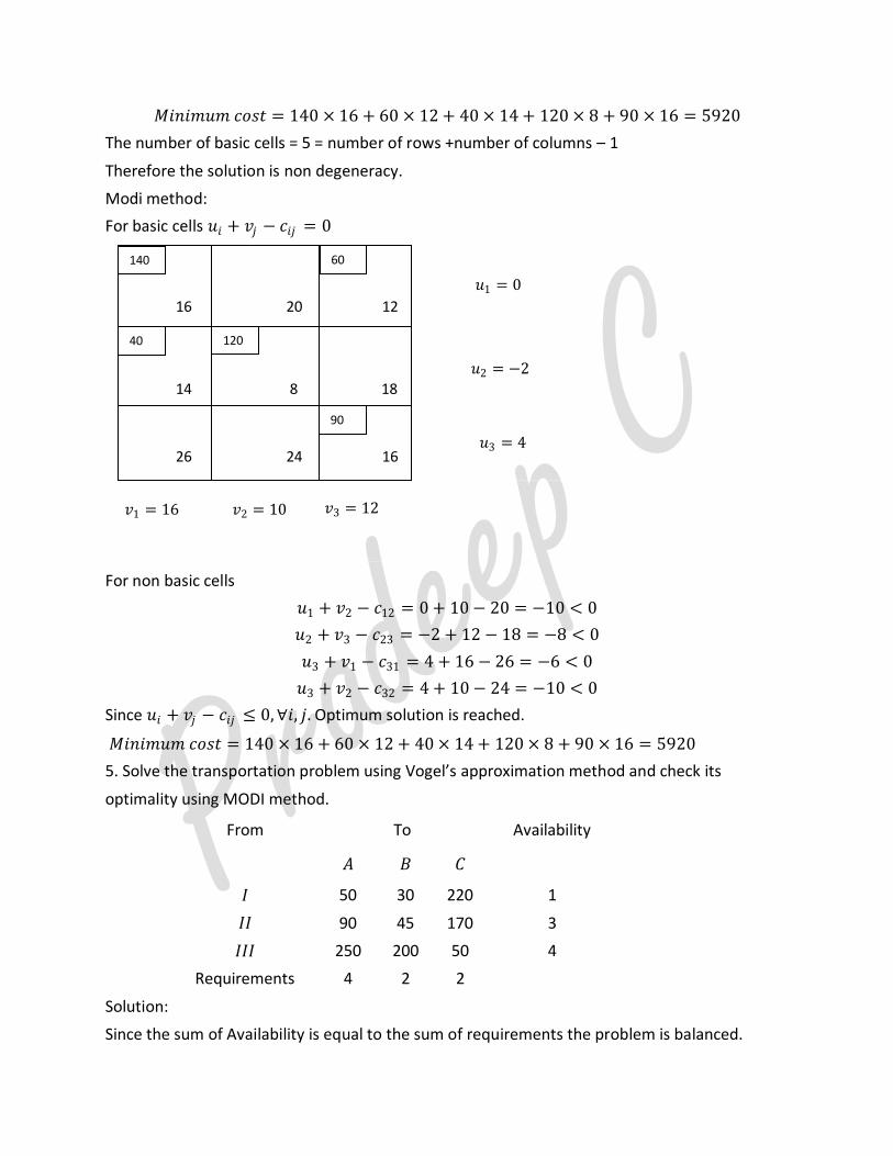
𝑀𝑖𝑛𝑖𝑚𝑢𝑚 𝑐𝑜𝑠𝑡 = 140 × 16 + 60 × 12 + 40 × 14 + 120 × 8 + 90 × 16 = 5920
The number of basic cells = 5 = number of rows +number of columns – 1
Therefore the solution is non degeneracy.
Modi method:
For basic cells 𝑢𝑖 + 𝑣𝑗 − 𝑐𝑖𝑗 = 0
For non basic cells
𝑢1 + 𝑣2 − 𝑐12 = 0 + 10 − 20 = −10 < 0
𝑢2 + 𝑣3 − 𝑐23 = −2 + 12 − 18 = −8 < 0
𝑢3 + 𝑣1 − 𝑐31 = 4 + 16 − 26 = −6 < 0
𝑢3 + 𝑣2 − 𝑐32 = 4 + 10 − 24 = −10 < 0
Since 𝑢𝑖 + 𝑣𝑗 − 𝑐𝑖𝑗 ≤ 0,∀𝑖, 𝑗. Optimum solution is reached.
𝑀𝑖𝑛𝑖𝑚𝑢𝑚 𝑐𝑜𝑠𝑡 = 140 × 16 + 60 × 12 + 40 × 14 + 120 × 8 + 90 × 16 = 5920
5. Solve the transportation problem using Vogel’s approximation method and check its
optimality using MODI method.
From To Availability
𝐴 𝐵 𝐶
𝐼 50 30 220 1
𝐼𝐼 90 45 170 3
𝐼𝐼𝐼 250 200 50 4
Requirements 4 2 2
Solution:
Since the sum of Availability is equal to the sum of requirements the problem is balanced.
16 20 12
14 8 18
26 24 16
𝑢1 = 0
𝑢2 = −2
𝑢3 = 4
𝑣1 = 16 𝑣2 = 10
120
90
𝑣3 = 12
60 140
40
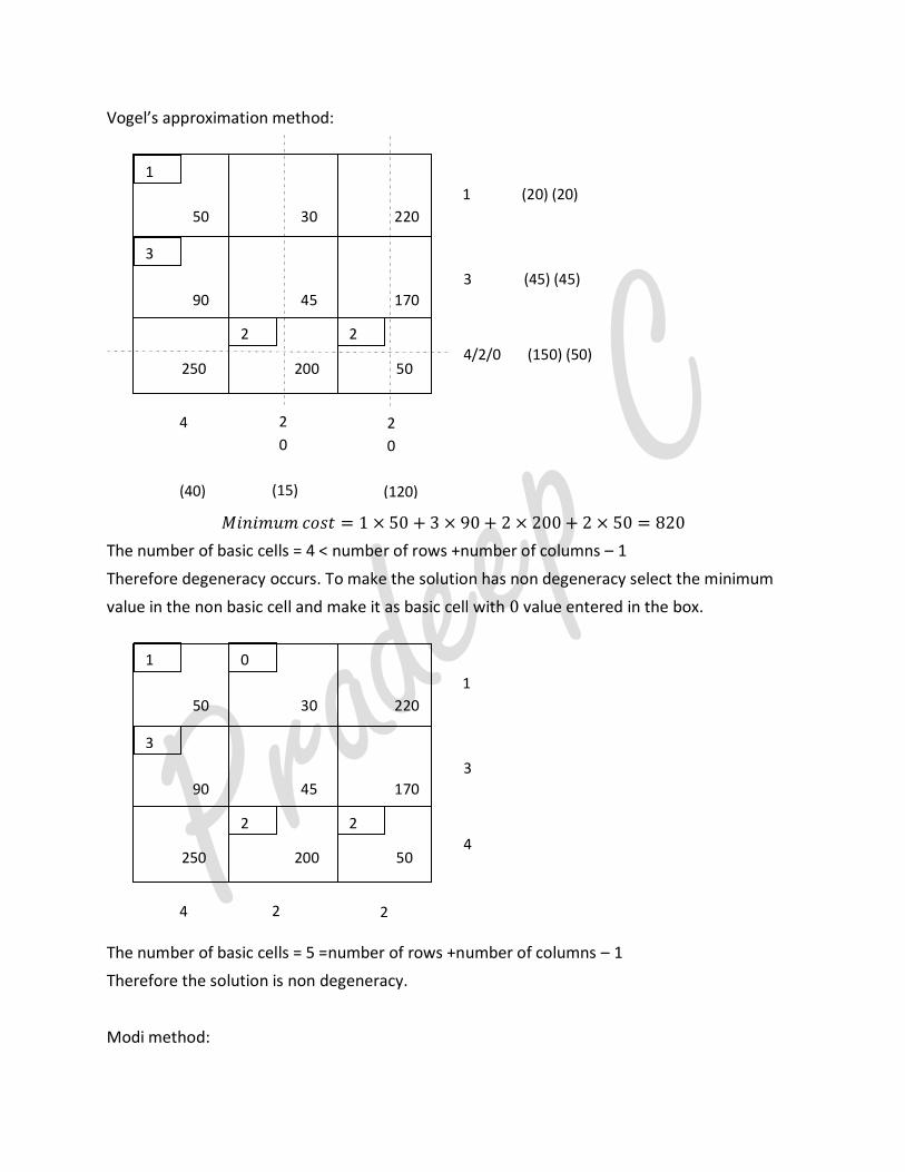
Vogel’s approximation method:
𝑀𝑖𝑛𝑖𝑚𝑢𝑚 𝑐𝑜𝑠𝑡 = 1 × 50 + 3 × 90 + 2 × 200 + 2 × 50 = 820
The number of basic cells = 4 < number of rows +number of columns – 1
Therefore degeneracy occurs. To make the solution has non degeneracy select the minimum
value in the non basic cell and make it as basic cell with 0 value entered in the box.
The number of basic cells = 5 =number of rows +number of columns – 1
Therefore the solution is non degeneracy.
Modi method:
50 30 220
90 45 170
250 200 50
1
3
4
4 2
2 2
1
3
2
0
50 30 220
90 45 170
250 200 50
1 (20) (20)
3 (45) (45)
4/2/0 (150) (50)
4
(40)
2
0
(15)
2 2
1
3
2
0
(120)

For basic cells 𝑢𝑖 + 𝑣𝑗 − 𝑐𝑖𝑗 = 0
For non basic cells
𝑢1 + 𝑣3 − 𝑐13 = 0 − 120 − 220 = −340 < 0
𝑢2 + 𝑣2 − 𝑐22 = 40 + 30 − 45 = 25 > 0
𝑢2 + 𝑣3 − 𝑐23 = 40 − 120 − 170 = −250 < 0
𝑢3 + 𝑣1 − 𝑐31 = 170 + 50 − 250 = −30 < 0
Put 𝜖 = 0, we get
2 2
1 + 𝜖
𝜖
0 − 𝜖
3 − 𝜖
50 30 220
90 45 170
250 200 50
50 30 220
90 45 170
250 200 50
𝑢1 = 0
2 2
1
3
0
𝑢2 = 40
𝑢3 = 170
𝑣3 = −120 𝑣2 = 30 𝑣1 = 50
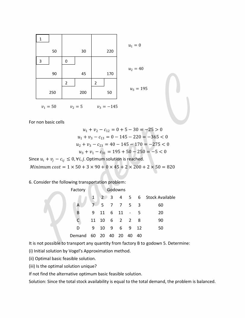
For non basic cells
𝑢1 + 𝑣2 − 𝑐12 = 0 + 5 − 30 = −25 > 0
𝑢1 + 𝑣3 − 𝑐13 = 0 − 145 − 220 = −365 < 0
𝑢2 + 𝑣3 − 𝑐23 = 40 − 145 − 170 = −275 < 0
𝑢3 + 𝑣1 − 𝑐31 = 195 + 50 − 250 = −5 < 0
Since 𝑢𝑖 + 𝑣𝑗 − 𝑐𝑖𝑗 ≤ 0,∀𝑖, 𝑗. Optimum solution is reached.
𝑀𝑖𝑛𝑖𝑚𝑢𝑚 𝑐𝑜𝑠𝑡 = 1 × 50 + 3 × 90 + 0 × 45 + 2 × 200 + 2 × 50 = 820
6. Consider the following transportation problem:
Factory Godowns
1 2 3 4 5 6 Stock Available
A 7 5 7 7 5 3 60
B 9 11 6 11 - 5 20
C 11 10 6 2 2 8 90
D 9 10 9 6 9 12 50
Demand 60 20 40 20 40 40
It is not possible to transport any quantity from factory B to godown 5. Determine:
(i) Initial solution by Vogel’s Approximation method.
(ii) Optimal basic feasible solution.
(iii) Is the optimal solution unique?
If not find the alternative optimum basic feasible solution.
Solution: Since the total stock availability is equal to the total demand, the problem is balanced.
50 30 220
90 45 170
250 200 50
𝑢1 = 0
2 2
1
3 0
𝑢2 = 40
𝑢3 = 195
𝑣3 = −145 𝑣2 = 5 𝑣1 = 50
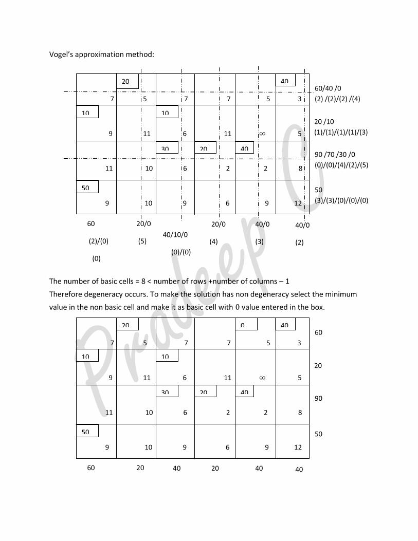
Vogel’s approximation method:
The number of basic cells = 8 < number of rows +number of columns – 1
Therefore degeneracy occurs. To make the solution has non degeneracy select the minimum
value in the non basic cell and make it as basic cell with 0 value entered in the box.
7 5 7 7 5 3
9 11 6 11 ∞ 5
11 10 6 2 2 8
9 10 9 6 9 12
60
60
20
40 20 40
20
90
50
20
30
40
10
40
40
20
10
50
0
7 5 7 7 5 3
9 11 6 11 ∞ 5
11 10 6 2 2 8
9 10 9 6 9 12
60
(2)/(0)
(0)
60/40 /0
(2) /(2)/(2) /(4)
20/0
(5)
40/10/0
(0)/(0)
(3)
20/0
(4)
40/0
(3)
20 /10
(1)/(1)/(1)/(1)/(3)
90 /70 /30 /0
(0)/(0)/(4)/(2)/(5)
50
(3)/(3)/(0)/(0)/(0)
20
30
40
10
40
40/0
(2)
20
10
50
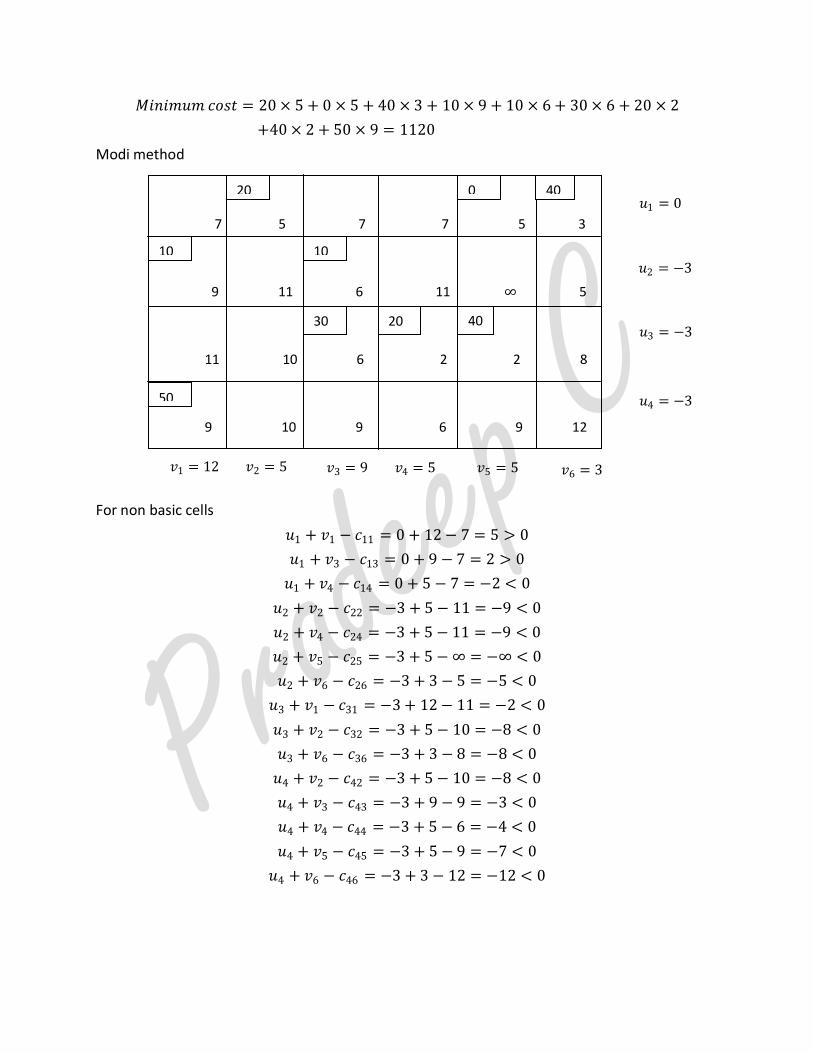
𝑀𝑖𝑛𝑖𝑚𝑢𝑚 𝑐𝑜𝑠𝑡 = 20 × 5 + 0 × 5 + 40 × 3 + 10 × 9 + 10 × 6 + 30 × 6 + 20 × 2
+40 × 2 + 50 × 9 = 1120
Modi method
For non basic cells
𝑢1 + 𝑣1 − 𝑐11 = 0 + 12 − 7 = 5 > 0
𝑢1 + 𝑣3 − 𝑐13 = 0 + 9 − 7 = 2 > 0
𝑢1 + 𝑣4 − 𝑐14 = 0 + 5 − 7 = −2 < 0
𝑢2 + 𝑣2 − 𝑐22 = −3 + 5 − 11 = −9 < 0
𝑢2 + 𝑣4 − 𝑐24 = −3 + 5 − 11 = −9 < 0
𝑢2 + 𝑣5 − 𝑐25 = −3 + 5 − ∞ = −∞ < 0
𝑢2 + 𝑣6 − 𝑐26 = −3 + 3 − 5 = −5 < 0
𝑢3 + 𝑣1 − 𝑐31 = −3 + 12 − 11 = −2 < 0
𝑢3 + 𝑣2 − 𝑐32 = −3 + 5 − 10 = −8 < 0
𝑢3 + 𝑣6 − 𝑐36 = −3 + 3 − 8 = −8 < 0
𝑢4 + 𝑣2 − 𝑐42 = −3 + 5 − 10 = −8 < 0
𝑢4 + 𝑣3 − 𝑐43 = −3 + 9 − 9 = −3 < 0
𝑢4 + 𝑣4 − 𝑐44 = −3 + 5 − 6 = −4 < 0
𝑢4 + 𝑣5 − 𝑐45 = −3 + 5 − 9 = −7 < 0
𝑢4 + 𝑣6 − 𝑐46 = −3 + 3 − 12 = −12 < 0
7 5 7 7 5 3
9 11 6 11 ∞ 5
11 10 6 2 2 8
9 10 9 6 9 12
𝑣1 = 12
𝑢1 = 0
𝑣2 = 5
𝑣3 = 9
𝑣4 = 5
𝑣5 = 5
𝑢2 = −3
𝑢3 = −3
𝑢4 = −3
20
30
40
10
40
𝑣6 = 3
20
10
50
0
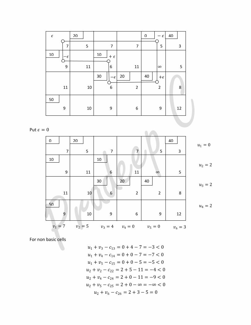
Put 𝜖 = 0
For non basic cells
𝑢1 + 𝑣3 − 𝑐13 = 0 + 4 − 7 = −3 < 0
𝑢1 + 𝑣4 − 𝑐14 = 0 + 0 − 7 = −7 < 0
𝑢1 + 𝑣5 − 𝑐15 = 0 + 0 − 5 = −5 < 0
𝑢2 + 𝑣2 − 𝑐22 = 2 + 5 − 11 = −4 < 0
𝑢2 + 𝑣4 − 𝑐24 = 2 + 0 − 11 = −9 < 0
𝑢2 + 𝑣5 − 𝑐25 = 2 + 0 − ∞ = −∞ < 0
𝑢2 + 𝑣6 − 𝑐26 = 2 + 3 − 5 = 0
7 5 7 7 5 3
9 11 6 11 ∞ 5
11 10 6 2 2 8
9 10 9 6 9 12
𝑣1 = 7
𝑢1 = 0
𝑣2 = 5
𝑣3 = 4
𝑣4 = 0
𝑣5 = 0
𝑢2 = 2
𝑢3 = 2
𝑢4 = 2
20
30
40
10
40
𝑣6 = 3
20
10
50
0
𝜖 − 𝜖
7 5 7 7 5 3
−𝜖 + 𝜖
9 11 6 11 ∞ 5
−𝜖 +𝜖
11 10 6 2 2 8
9 10 9 6 9 12
20
30
40
10
40 20
10
50
0
𝑢3 + 𝑣1 − 𝑐31 = 2 + 7 − 11 = −2 < 0
𝑢3 + 𝑣2 − 𝑐32 = 2 + 5 − 10 = −3 < 0
𝑢3 + 𝑣6 − 𝑐36 = 2 + 3 − 8 = −3 < 0
𝑢4 + 𝑣2 − 𝑐42 = 2 + 5 − 10 = −3 < 0
𝑢4 + 𝑣3 − 𝑐43 = 2 + 4 − 9 = −3 < 0
𝑢4 + 𝑣4 − 𝑐44 = 2 + 0 − 6 = −4 < 0
𝑢4 + 𝑣5 − 𝑐45 = 2 + 0 − 9 = −7 < 0
𝑢4 + 𝑣6 − 𝑐46 = 2 + 3 − 12 = −7 < 0
Since 𝑢𝑖 + 𝑣𝑗 − 𝑐𝑖𝑗 ≤ 0,∀𝑖, 𝑗. Optimum solution is reached.
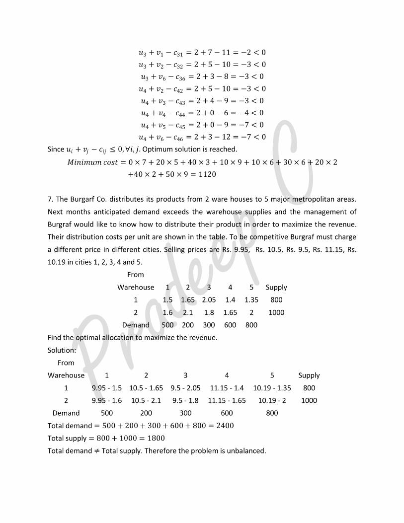
𝑀𝑖𝑛𝑖𝑚𝑢𝑚 𝑐𝑜𝑠𝑡 = 0 × 7 + 20 × 5 + 40 × 3 + 10 × 9 + 10 × 6 + 30 × 6 + 20 × 2
+40 × 2 + 50 × 9 = 1120
7. The Burgarf Co. distributes its products from 2 ware houses to 5 major metropolitan areas.
Next months anticipated demand exceeds the warehouse supplies and the management of
Burgraf would like to know how to distribute their product in order to maximize the revenue.
Their distribution costs per unit are shown in the table. To be competitive Burgraf must charge
a different price in different cities. Selling prices are Rs. 9.95, Rs. 10.5, Rs. 9.5, Rs. 11.15, Rs.
10.19 in cities 1, 2, 3, 4 and 5.
From
Warehouse 1 2 3 4 5 Supply
1 1.5 1.65 2.05 1.4 1.35 800
2 1.6 2.1 1.8 1.65 2 1000
Demand 500 200 300 600 800
Find the optimal allocation to maximize the revenue.
Solution:
From
Warehouse 1 2 3 4 5 Supply
1 9.95 - 1.5 10.5 - 1.65 9.5 - 2.05 11.15 - 1.4 10.19 - 1.35 800
2 9.95 - 1.6 10.5 - 2.1 9.5 - 1.8 11.15 - 1.65 10.19 - 2 1000
Demand 500 200 300 600 800
Total demand = 500 + 200 + 300 + 600 + 800 = 2400
Total supply = 800 + 1000 = 1800
Total demand ≠ Total supply. Therefore the problem is unbalanced.
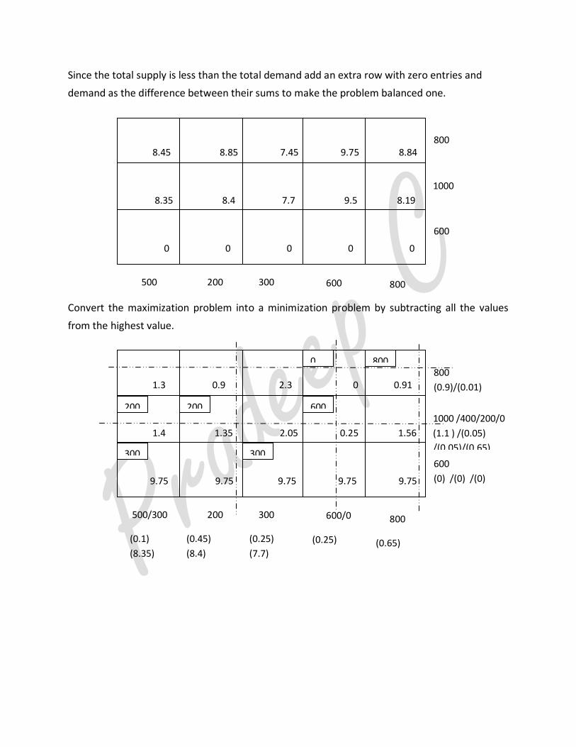
Since the total supply is less than the total demand add an extra row with zero entries and
demand as the difference between their sums to make the problem balanced one.
Convert the maximization problem into a minimization problem by subtracting all the values
from the highest value.
1.3 0.9 2.3 0 0.91
1.4 1.35 2.05 0.25 1.56
9.75 9.75 9.75 9.75 9.75
500/300
(0.1)
(8.35)
800
(0.9)/(0.01)
200
(0.45)
(8.4)
300
(0.25)
(7.7)
600/0
(0.25)
800
(0.65)
1000 /400/200/0
(1.1 ) /(0.05)
/(0.05)/(0.65)
600
(0) /(0) /(0)
600 200 200
800 0
300 300
8.45 8.85 7.45 9.75 8.84
8.35 8.4 7.7 9.5 8.19
0 0 0 0 0
9 11 13 8 0
500
800
200
300 600 800
1000
600
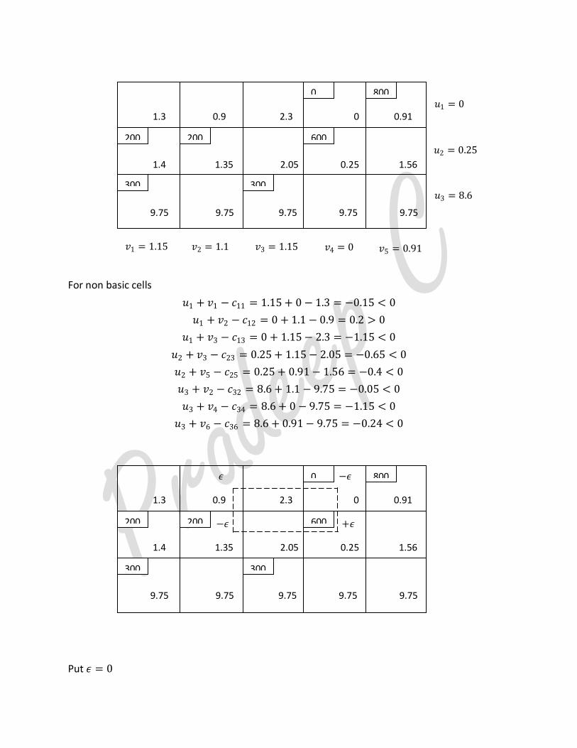
For non basic cells
𝑢1 + 𝑣1 − 𝑐11 = 1.15 + 0 − 1.3 = −0.15 < 0
𝑢1 + 𝑣2 − 𝑐12 = 0 + 1.1 − 0.9 = 0.2 > 0
𝑢1 + 𝑣3 − 𝑐13 = 0 + 1.15 − 2.3 = −1.15 < 0
𝑢2 + 𝑣3 − 𝑐23 = 0.25 + 1.15 − 2.05 = −0.65 < 0
𝑢2 + 𝑣5 − 𝑐25 = 0.25 + 0.91 − 1.56 = −0.4 < 0
𝑢3 + 𝑣2 − 𝑐32 = 8.6 + 1.1 − 9.75 = −0.05 < 0
𝑢3 + 𝑣4 − 𝑐34 = 8.6 + 0 − 9.75 = −1.15 < 0
𝑢3 + 𝑣6 − 𝑐36 = 8.6 + 0.91 − 9.75 = −0.24 < 0
Put 𝜖 = 0
𝜖 −𝜖
1.3 0.9 2.3 0 0.91
−𝜖 +𝜖
1.4 1.35 2.05 0.25 1.56
9.75 9.75 9.75 9.75 9.75
600 200 200
800 0
300 300
1.3 0.9 2.3 0 0.91
1.4 1.35 2.05 0.25 1.56
9.75 9.75 9.75 9.75 9.75
𝑣1 = 1.15
𝑢1 = 0
𝑣2 = 1.1 𝑣3 = 1.15 𝑣4 = 0 𝑣5 = 0.91
𝑢2 = 0.25
𝑢3 = 8.6
600 200 200
800 0
300 300

For non basic cells
𝑢1 + 𝑣1 − 𝑐11 = 0 + 0.95 − 1.3 = −0.35 < 0
𝑢1 + 𝑣3 − 𝑐13 = 0 + 0.95 − 2.3 = −1.35 < 0
𝑢1 + 𝑣4 − 𝑐14 = 0 − 0.2 − 0 = −0.2 < 0
𝑢2 + 𝑣3 − 𝑐23 = 0.45 + 0.95 − 2.05 = −0.65 < 0
𝑢2 + 𝑣5 − 𝑐25 = 0.45 + 0.91 − 1.56 = −0.2 < 0
𝑢3 + 𝑣2 − 𝑐32 = 8.8 + 0.9 − 9.75 = −0.05 < 0
𝑢3 + 𝑣4 − 𝑐34 = 8.8 − 0.2 − 9.75 = −1.15 < 0
𝑢3 + 𝑣6 − 𝑐36 = 8.8 + 0.91 − 9.75 = −0.04 < 0
Since 𝑢𝑖 + 𝑣𝑗 − 𝑐𝑖𝑗 ≤ 0,∀𝑖, 𝑗. Optimum solution is reached.
𝑀𝑎𝑥𝑖𝑚𝑢𝑚 𝑐𝑜𝑠𝑡 = 0 × 8.85 + 800 × 8.84 + 200 × 8.35 + 200 × 8.4 + 600 × 9.5
+300 × 0 + 300 × 0 = 16122
8.45 8.85 7.45 9.75 8.84
8.35 8.4 7.7 9.5 8.19
0 0 0 0 0
9 11 13 8 0
500
800
200
300 600 800
1000
600
0 800
200 200 600
300 300
1.3 0.9 2.3 0 0.91
1.4 1.35 2.05 0.25 1.56
9.75 9.75 9.75 9.75 9.75
𝑣1 = 0.95
𝑢1 = 0
𝑣2 = 0.9 𝑣3 = 0.95 𝑣4 = −0.2 𝑣5 = 0.91
𝑢2 = 0.45
𝑢3 = 8.8
600 200 200
800 0
300 300
Assignment Problem
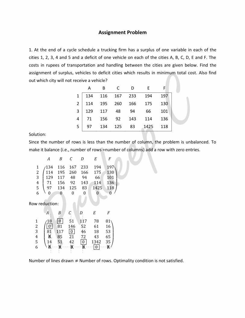
1. At the end of a cycle schedule a trucking firm has a surplus of one variable in each of the
cities 1, 2, 3, 4 and 5 and a deficit of one vehicle on each of the cities A, B, C, D, E and F. The
costs in rupees of transportation and handling between the cities are given below. Find the
assignment of surplus, vehicles to deficit cities which results in minimum total cost. Also find
out which city will not receive a vehicle?
A B C D E F
1 134 116 167 233 194 197
2 114 195 260 166 175 130
3 129 117 48 94 66 101
4 71 156 92 143 114 136
5 97 134 125 83 1425 118
Solution:
Since the number of rows is less than the number of column, the problem is unbalanced. To
make it balance (i.e., number of rows =number of columns) add a row with zero entries.
Row reduction:
Number of lines drawn ≠ Number of rows. Optimality condition is not satisfied.
18 0 51 117 78 810 81 146 52 61 16
81 117 0 46 18 530 85 21 72 43 65
14 51 42 0 1342 350 0 0 0 0 0
𝐴 𝐵 𝐶 𝐷 𝐸 𝐹
123456
134 116 167 233 194 197114 195 260 166 175 130129 117 48 94 66 10171 156 92 143 114 13697 134 125 83 1425 1180 0 0 0 0 0
𝐴 𝐵 𝐶 𝐷 𝐸 𝐹
123456
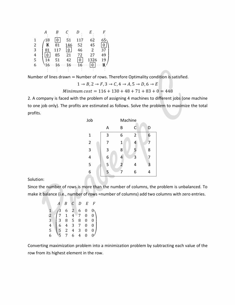
Number of lines drawn = Number of rows. Therefore Optimality condition is satisfied.
1 → 𝐵, 2 → 𝐹, 3 → 𝐶, 4 → 𝐴, 5 → 𝐷, 6 → 𝐸
𝑀𝑖𝑛𝑖𝑚𝑢𝑚 𝑐𝑜𝑠𝑡 = 116 + 130 + 48 + 71 + 83 + 0 = 448
2. A company is faced with the problem of assigning 4 machines to different jobs (one machine
to one job only). The profits are estimated as follows. Solve the problem to maximize the total
profits.
Job Machine
A B C D
1 3 6 2 6
2 7 1 4 7
3 3 8 5 8
4 6 4 3 7
5 5 2 4 3
6 5 7 6 4
Solution:
Since the number of rows is more than the number of columns, the problem is unbalanced. To
make it balance (i.e., number of rows =number of columns) add two columns with zero entries.
Converting maximization problem into a minimization problem by subtracting each value of the
row from its highest element in the row.
3 6 2 6 0 07 1 4 7 0 03 8 5 8 0 06 4 3 7 0 05 2 4 3 0 05 7 6 4 0 0
𝐴 𝐵 𝐶 𝐷 𝐸 𝐹
123456
𝐴 𝐵 𝐶 𝐷 𝐸 𝐹
123456
18 0 51 117 62 650 81 146 52 45 0
81 117 0 46 2 370 85 21 72 27 49
14 51 42 0 1326 1916 16 16 16 0 0
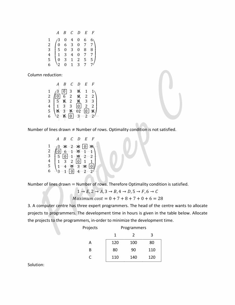
Column reduction:
Number of lines drawn ≠ Number of rows. Optimality condition is not satisfied.
Number of lines drawn = Number of rows. Therefore Optimality condition is satisfied.
1 → 𝐸, 2 → 𝐴, 3 → 𝐵, 4 → 𝐷, 5 → 𝐹, 6 → 𝐶
𝑀𝑎𝑥𝑖𝑚𝑢𝑚 𝑐𝑜𝑠𝑡 = 0 + 7 + 8 + 7 + 0 + 6 = 28
3. A computer centre has three expert programmers. The head of the centre wants to allocate
projects to programmers. The development time in hours is given in the table below. Allocate
the projects to the programmers, in-order to minimize the development time.
Projects Programmers
1 2 3
A 120 100 80
B 80 90 110
C 110 140 120
Solution:
𝐴 𝐵 𝐶 𝐷 𝐸 𝐹
123456
3 0 2 0 0 00 6 1 0 1 15 0 1 0 2 21 3 2 0 1 11 4 0 3 0 03 1 0 4 2 2
3 0 3 0 1 10 6 2 0 2 25 0 2 0 3 31 3 3 0 2 20 3 0 02 0 02 0 0 3 2 2
𝐴 𝐵 𝐶 𝐷 𝐸 𝐹
123456
3 0 4 0 6 60 6 3 0 7 75 0 3 0 8 81 3 4 0 7 70 3 1 2 5 52 0 1 3 7 7
𝐴 𝐵 𝐶 𝐷 𝐸 𝐹
123456
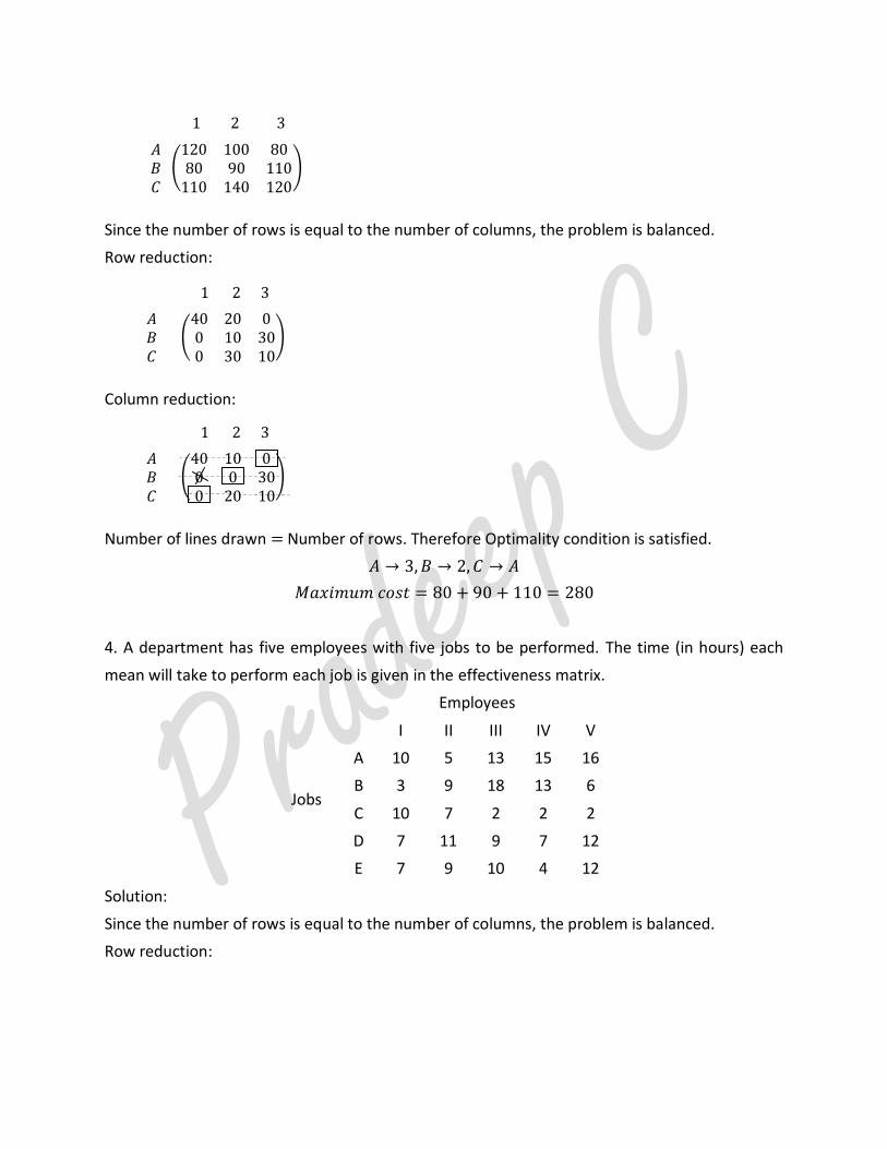
Since the number of rows is equal to the number of columns, the problem is balanced.
Row reduction:
Column reduction:
Number of lines drawn = Number of rows. Therefore Optimality condition is satisfied.
𝐴 → 3,𝐵 → 2,𝐶 → 𝐴
𝑀𝑎𝑥𝑖𝑚𝑢𝑚 𝑐𝑜𝑠𝑡 = 80 + 90 + 110 = 280
4. A department has five employees with five jobs to be performed. The time (in hours) each
mean will take to perform each job is given in the effectiveness matrix.
Employees
Jobs
I II III IV V
A 10 5 13 15 16
B 3 9 18 13 6
C 10 7 2 2 2
D 7 11 9 7 12
E 7 9 10 4 12
Solution:
Since the number of rows is equal to the number of columns, the problem is balanced.
Row reduction:
40 10 00 0 300 20 10
1 2 3
𝐴𝐵𝐶
40 20 00 10 300 30 10
1 2 3
𝐴𝐵𝐶
120 100 8080 90 110
110 140 120
1 2 3
𝐴𝐵𝐶
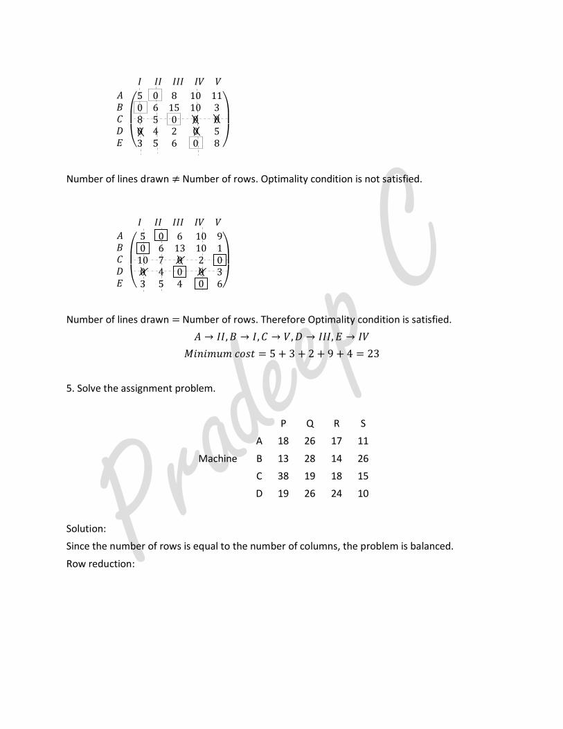
Number of lines drawn ≠ Number of rows. Optimality condition is not satisfied.
Number of lines drawn = Number of rows. Therefore Optimality condition is satisfied.
𝐴 → 𝐼𝐼,𝐵 → 𝐼,𝐶 → 𝑉,𝐷 → 𝐼𝐼𝐼, 𝐸 → 𝐼𝑉
𝑀𝑖𝑛𝑖𝑚𝑢𝑚 𝑐𝑜𝑠𝑡 = 5 + 3 + 2 + 9 + 4 = 23
5. Solve the assignment problem.
Machine
P Q R S
A 18 26 17 11
B 13 28 14 26
C 38 19 18 15
D 19 26 24 10
Solution:
Since the number of rows is equal to the number of columns, the problem is balanced.
Row reduction:
5 0 6 10 90 6 13 10 1
10 7 0 2 00 4 0 0 33 5 4 0 6
𝐼 𝐼𝐼 𝐼𝐼𝐼 𝐼𝑉 𝑉
𝐴𝐵𝐶𝐷𝐸
5 0 8 10 110 6 15 10 38 5 0 0 00 4 2 0 53 5 6 0 8
𝐼 𝐼𝐼 𝐼𝐼𝐼 𝐼𝑉 𝑉
𝐴𝐵𝐶𝐷𝐸

Column reduction:
Number of lines drawn ≠ Number of rows. Optimality condition is not satisfied.
Number of lines drawn ≠ Number of rows. Optimality condition is not satisfied.
Number of lines drawn = Number of rows. Therefore Optimality condition is satisfied.
𝐴 → 𝑅,𝐵 → 𝑃, 𝐶 → 𝑄,𝐷 → 𝑆
𝑀𝑖𝑛𝑖𝑚𝑢𝑚 𝑐𝑜𝑠𝑡 = 17 + 13 + 19 + 10 = 59
𝑃 𝑄 𝑅 𝑆
𝐴𝐵𝐶𝐷
2 8 0 00 13 0 18
21 0 0 34 9 8 0
𝑃 𝑄 𝑅 𝑆
𝐴𝐵𝐶𝐷
5 11 3 00 13 0 15
21 0 0 07 12 11 0
7 11 5 00 11 0 13
23 0 2 09 12 13 0
𝑃 𝑄 𝑅 𝑆
𝐴𝐵𝐶𝐷
7 15 6 00 15 1 13
23 4 3 09 16 14 0
𝑃 𝑄 𝑅 𝑆
𝐴𝐵𝐶𝐷
6. A company has five jobs to be done. The following matrix shows the return in rupees of
assigning 𝑖𝑡ℎ machine 𝑖 = 1, 2, 3, 4, 5 to the 𝑗𝑡ℎ job 𝑗 = 𝐴, 𝐵,𝐶 ,𝐷, 𝐸 . Assign the five jobs to
the five machines to maximize profit.
A B C D E
1 5 11 10 12 4
2 2 4 6 3 5
3 3 12 5 14 6
4 6 14 4 11 7
5 7 9 8 12 5
Solution:
Since the number of rows is equal to the number of columns, the problem is balanced.
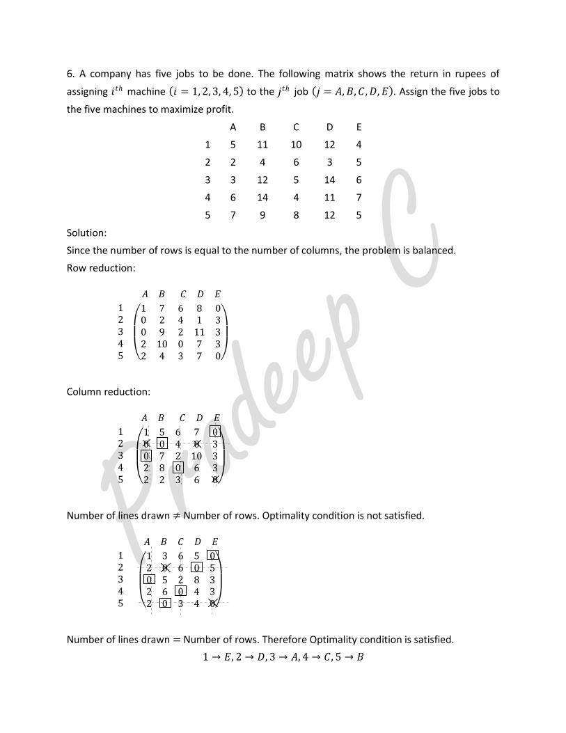
Row reduction:
Column reduction:
Number of lines drawn ≠ Number of rows. Optimality condition is not satisfied.
Number of lines drawn = Number of rows. Therefore Optimality condition is satisfied.
1 → 𝐸, 2 → 𝐷, 3 → 𝐴, 4 → 𝐶, 5 → 𝐵
1 3 6 5 02 0 6 0 50 5 2 8 32 6 0 4 32 0 3 4 0
𝐴 𝐵 𝐶 𝐷 𝐸
12345
1 5 6 7 00 0 4 0 30 7 2 10 32 8 0 6 32 2 3 6 0
𝐴 𝐵 𝐶 𝐷 𝐸
12345
1 7 6 8 00 2 4 1 30 9 2 11 32 10 0 7 32 4 3 7 0
𝐴 𝐵 𝐶 𝐷 𝐸
12345
𝑀𝑖𝑛𝑖𝑚𝑢𝑚 𝑐𝑜𝑠𝑡 = 4 + 3 + 3 + 4 + 9 = 23
Travelling Salesman Problem
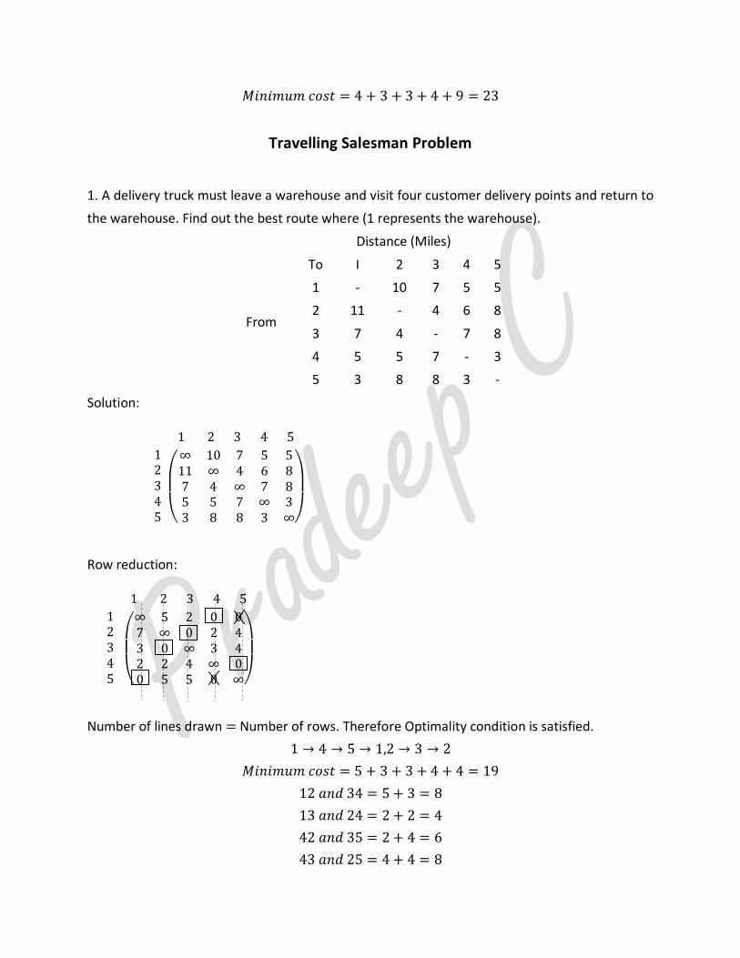
1. A delivery truck must leave a warehouse and visit four customer delivery points and return to
the warehouse. Find out the best route where (1 represents the warehouse).
Distance (Miles)
From
To I 2 3 4 5
1 - 10 7 5 5
2 11 - 4 6 8
3 7 4 - 7 8
4 5 5 7 - 3
5 3 8 8 3 -
Solution:
Row reduction:
Number of lines drawn = Number of rows. Therefore Optimality condition is satisfied.
1 → 4 → 5 → 1,2 → 3 → 2
𝑀𝑖𝑛𝑖𝑚𝑢𝑚 𝑐𝑜𝑠𝑡 = 5 + 3 + 3 + 4 + 4 = 19
12 𝑎𝑛𝑑 34 = 5 + 3 = 8
13 𝑎𝑛𝑑 24 = 2 + 2 = 4
42 𝑎𝑛𝑑 35 = 2 + 4 = 6
43 𝑎𝑛𝑑 25 = 4 + 4 = 8
∞ 5 2 0 07 ∞ 0 2 43 0 ∞ 3 42 2 4 ∞ 00 5 5 0 ∞
1 2 3 4 5
12345
∞ 10 7 5 511 ∞ 4 6 87 4 ∞ 7 85 5 7 ∞ 33 8 8 3 ∞
1 2 3 4 5
12345
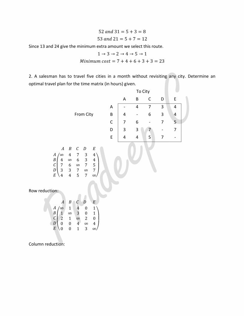
52 𝑎𝑛𝑑 31 = 5 + 3 = 8
53 𝑎𝑛𝑑 21 = 5 + 7 = 12
Since 13 and 24 give the minimum extra amount we select this route.
1 → 3 → 2 → 4 → 5 → 1
𝑀𝑖𝑛𝑖𝑚𝑢𝑚 𝑐𝑜𝑠𝑡 = 7 + 4 + 6 + 3 + 3 = 23
2. A salesman has to travel five cities in a month without revisiting any city. Determine an
optimal travel plan for the time matrix (in hours) given.
From City
To City
A B C D E
A - 4 7 3 4
B 4 - 6 3 4
C 7 6 - 7 5
D 3 3 7 - 7
E 4 4 5 7 -
Row reduction:
Column reduction:
∞ 1 4 0 11 ∞ 3 0 12 1 ∞ 2 00 0 4 ∞ 40 0 1 3 ∞
𝐴 𝐵 𝐶 𝐷 𝐸
𝐴𝐵𝐶𝐷𝐸
∞ 4 7 3 44 ∞ 6 3 47 6 ∞ 7 53 3 7 ∞ 74 4 5 7 ∞
𝐴 𝐵 𝐶 𝐷 𝐸
𝐴𝐵𝐶𝐷𝐸
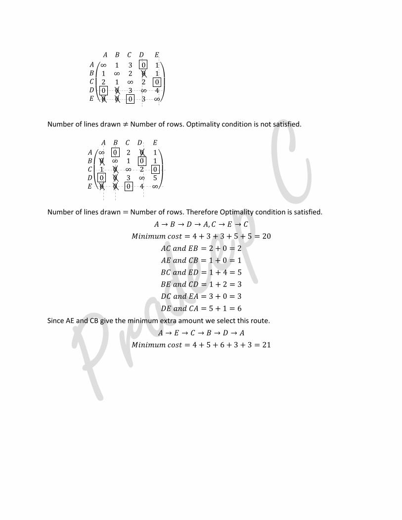
Number of lines drawn ≠ Number of rows. Optimality condition is not satisfied.
Number of lines drawn = Number of rows. Therefore Optimality condition is satisfied.
𝐴 → 𝐵 → 𝐷 → 𝐴, 𝐶 → 𝐸 → 𝐶
𝑀𝑖𝑛𝑖𝑚𝑢𝑚 𝑐𝑜𝑠𝑡 = 4 + 3 + 3 + 5 + 5 = 20
𝐴𝐶 𝑎𝑛𝑑 𝐸𝐵 = 2 + 0 = 2
𝐴𝐸 𝑎𝑛𝑑 𝐶𝐵 = 1 + 0 = 1
𝐵𝐶 𝑎𝑛𝑑 𝐸𝐷 = 1 + 4 = 5
𝐵𝐸 𝑎𝑛𝑑 𝐶𝐷 = 1 + 2 = 3
𝐷𝐶 𝑎𝑛𝑑 𝐸𝐴 = 3 + 0 = 3
𝐷𝐸 𝑎𝑛𝑑 𝐶𝐴 = 5 + 1 = 6
Since AE and CB give the minimum extra amount we select this route.
𝐴 → 𝐸 → 𝐶 → 𝐵 → 𝐷 → 𝐴
𝑀𝑖𝑛𝑖𝑚𝑢𝑚 𝑐𝑜𝑠𝑡 = 4 + 5 + 6 + 3 + 3 = 21
∞ 0 2 0 10 ∞ 1 0 11 0 ∞ 2 00 0 3 ∞ 50 0 0 4 ∞
𝐴 𝐵 𝐶 𝐷 𝐸
𝐴𝐵𝐶𝐷𝐸
∞ 1 3 0 11 ∞ 2 0 12 1 ∞ 2 00 0 3 ∞ 40 0 0 3 ∞
𝐴 𝐵 𝐶 𝐷 𝐸
𝐴𝐵𝐶𝐷𝐸


![Transportation Problem - ULisboaweb.tecnico.ulisboa.pt/~mcasquilho/CD_Casquilho/PRINT/...Transportation Problem [:8] 3 Any problem having the above structurecan beconsidered a TP,](https://img.dokumen.tips/doc/110x75/5e753e5b11ea724b977b7d81/transportation-problem-mcasquilhocdcasquilhoprint-transportation-problem.jpg)


