Embed Size (px)
Citation preview

Related Documents:
< FY 2007-2012 Transportation Improvement Program for Northeastern Illinois
< 2030 Regional Transportation Plan
< 2030 RTP Update to the Capital Element
< FY 2007-2012 TIP Project Listing
< Conformity Analysis
< Conformity Analysis - Appendix A
< Public Comment and Response
Transportation Conformity Analysis
Appendix BAdopted by the Chicago Area Transportation Study Policy Committee, October 12, 2006
For the PM2.5
and 8-Hour Ozone National Ambient Air Quality Standards

CATS POLICY COMMITTEE STATE TIMOTHY W. MARTIN, Chairman Secretary Illinois Department of Transportation REGIONAL STEPHEN E. SCHLICKMAN Executive Director Regional Transportation Authority EDWARD PAESEL Commissioner Northeastern Illinois Planning Commission LOCAL GOVERNMENTS JEFFERY SCHIELKE Mayor, City of Batavia CATS Council of Mayors CHERI HERAMB Acting Commissioner Chicago Department of Transportation JAMES ELDRIDGE, JR. Chief Administrative Officer Cook County TOM CUCULICH Director of Economic Development and Transportation Planning DuPage County KAREN McCONNAUGHAY County Board Chairman Kane County MARTIN G. BUEHLER Director of Transportation / County Engineer Lake County KENNETH D. KOEHLER County Board Chairman McHenry County SHELDON LATZ County Engineer Will County
ANNE VICKERY District 2 County Board Member Kendall County TRANSPORTATION OPERATORS FRANK KRUESI President Chicago Transit Authority MICHAEL W. PAYETTE Vice President Union Pacific Railroad Class 1 Railroad Companies PHILIP A. PAGANO Executive Director Commuter Rail Division of the RTA – Metra JOHN D. RITA South Suburban Mass Transit District Mass Transit Districts JOHN McCARTHY President, Continental Airport Express Private Transportation Providers JOHN J. CASE Chairman of the Board Suburban Bus Division of the RTA – Pace ROCCO J. ZUCCHERO Deputy Chief of Engineering for Planning Illinois State Toll Highway Authority FEDERAL AGENCIES NORMAN R. STONER Division Administrator Federal Highway Administration MARISOL SIMON Regional Administrator Federal Transit Administration SECRETARY DONALD P. KOPEC Executive Director Chicago Area Transportation Study

TRANSPORTATION CONFORMITY ANALYSIS FOR THE PM2.5 AND 8-HOUR OZONE
NATIONAL AMBIENT AIR QUALITY STANDARDS
2030 REGIONAL TRANSPORTATION PLAN
FY 2007-2012 TRANSPORTATION IMPROVEMENT PROGRAM
Appendix B Travel Demand Modeling for the
Conformity Process in Northeastern Illinois
Adopted by the Chicago Area Transportation Study Policy Committee – October 12, 2006
Prepared by Chicago Area Transportation Study
Chicago Metropolitan Agency for Planning 233 South Wacker Drive, Sears Tower
Chicago, IL 60606 (312) 454-0400


Transportation Conformity Analysis
Appendix B - i October 2006
Table of Contents TABLE OF CONTENTS ............................................................................................................................................ I
1 INTRODUCTION ...................................................................................................................................................1
2 HIGHWAY NETWORK ........................................................................................................................................7
3 TRANSIT NETWORK .........................................................................................................................................18
4 TRIP GENERATION ...........................................................................................................................................26
5 TRIP DISTRIBUTION .........................................................................................................................................48
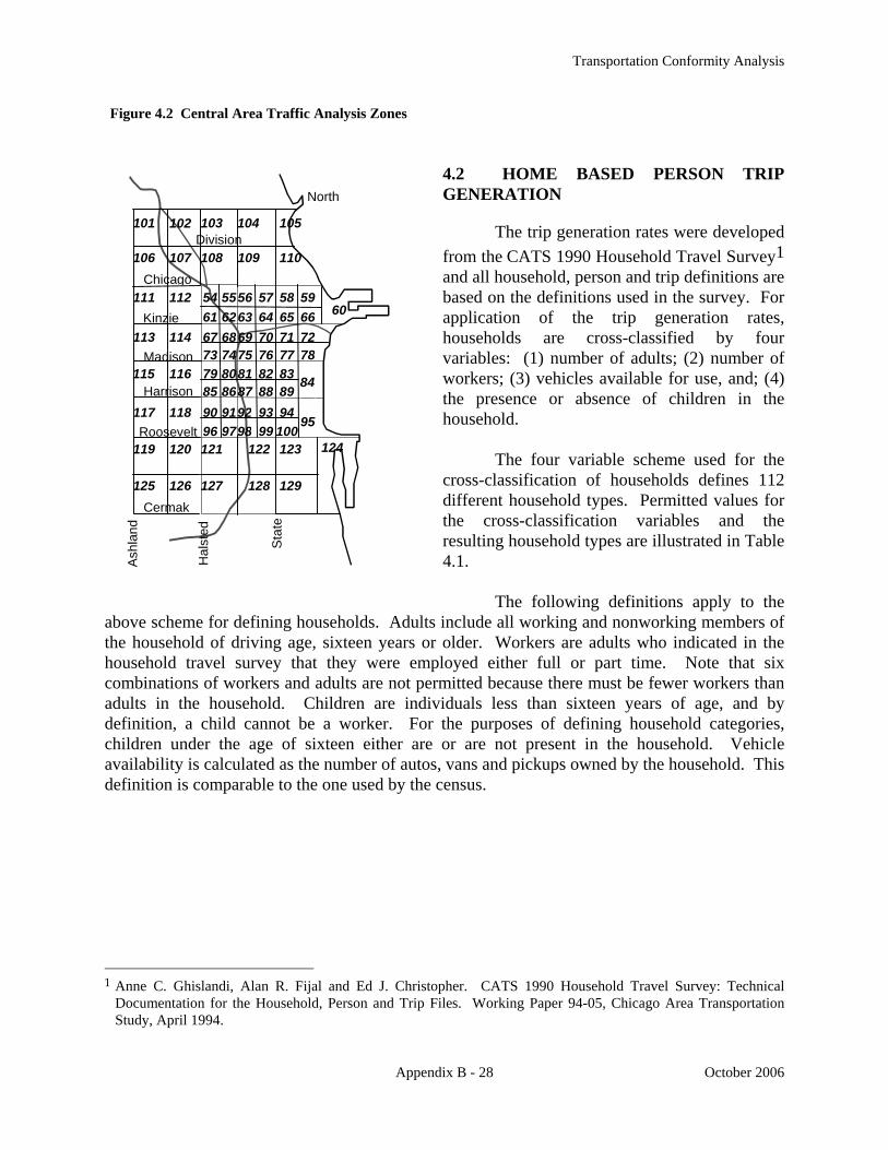
6 MODE CHOICE ...................................................................................................................................................63
7 TIME OF DAY HIGHWAY ASSIGNMENT......................................................................................................70
8 EMISSIONS CALCULATION.............................................................................................................................87


Transportation Conformity Analysis
Appendix B - 1 October 2006
1 INTRODUCTION The northeastern Illinois region is a moderate nonattainment area for the 8-hour ozone
standard under the Clean Air Act Amendments of 1990, and a nonattainment area for fine particulate matter (PM2.5). Provisions of this act require regional transportation plans and programs to conform to the State Implementation Plan (SIP) for air quality, which sets out how the region will meet emission reduction targets specified by the act. In advance of an approved SIP or emissions budgets, interim tests are required. This is the case with the PM2.5 standard; the tests required to demonstrate conformity in this case are described in further detail in the main body of the document.
The travel demand models, and emission calculations that depend on the models' travel
forecasts, are the technical core of the conformity evaluations of the region's Transportation Improvement Program (TIP) and Regional Transportation Plan (RTP). The purpose of this report is to document the travel demand modeling process used in the conformity analysis. The Chicago Area Transportation Study (CATS) is the primary agency for the development and maintenance of travel forecasting methods for the Chicago region. CATS has been developing and improving these travel forecasting procedures constantly since 1956. The present set of models was originally developed using a 1970 home interview survey. This survey obtained the daily travel patterns for over 21,000 households in the region. The original CATS home interview survey was taken in 1956 and consisted of almost 40,000 household interviews.
In 1979 a much smaller home interview was conducted and this survey and the 1980 Census Journey to Work data was used to review and modify the procedures. Between 1988 and 1991 another large-scale home interview survey (over 19,000 households) was conducted. The information from this survey and the 1990 Census has been used to update and modify the travel demand procedures. In addition to these home interview surveys, there have been several other data collection efforts, including a 1986 Commercial Vehicle Survey, a 1963 pedestrian survey, a 1987 survey of parkers in the Chicago Central Business District, and a 1991 survey of parking spaces in the central Business District, which have been used to enhance the travel demand procedures. For most of the last decade, CATS has been working to enhance the travel demand modeling process used in the air quality conformity analysis of transportation improvement programs and regional transportation plans. This chapter describes the general structure of the modeling process and highlights improvements that have recently been made. Subsequent chapters concentrate on particular model steps. Travel demand modeling was first employed to assist in the development of regional transportation plans. The four-step process (trip generation, distribution, mode split and assignment) was fundamental from the beginning. Early enhancements focused on making the process run more quickly on the computers available at the time and on the calibration of individual model components. In the seventies, in response to concerns about improving public
Transportation Conformity Analysis
Appendix B - 2 October 2006
transit, CATS concentrated enhancement activities on the mode split model and transit assignment techniques. In the late seventies and eighties, efforts were focused on adapting the modeling process to sub-area and project specific studies. For example, CATS developed a block by block zone system for the downtown area. Trips were generated based on zonal floor space from a building by building file of the area. Networks were coded with detailed pedestrian links. These techniques were employed to evaluate transit alternatives for the CBD area. Similarly, zone sizes were reduced and more detailed highway networks coded in suburban areas to evaluate freeway proposals. When the federal regulations were changed to require emissions estimates for conformity analysis, the regional models were initially employed as they then existed. It was in 1994 that the first significant model changes, explicitly motivated by conformity issues, were implemented. Since then, CATS has committed substantial resources to develop models that are responsive to needs imposed by air quality requirements. The CATS travel demand models represent a classical "four-step" process of trip generation, distribution, mode choice, and assignment, with considerable modifications used to enhance the distribution and mode choice procedures. The present CATS region, for analysis purposes, includes the counties of Lake, McHenry, Cook, DuPage, Kankakee, Kane, Kendall, Grundy, and Will in Illinois, and Lake County in Indiana and parts of other Illinois, Indiana and Wisconsin counties buffering the region. Figure 1.1 contains a flow diagram showing the general steps used in the travel demand estimation procedures. The ovals on the chart are data files. The rectangles are models or processes. The first step in the procedure is to use the socioeconomic/land use data to estimate the trip ends for each trip type. These trip ends are defined as productions, which for home based trips are the trip ends located at the traveler's home, and attractions, which are the trip ends located at the non-home end of the traveler. This model step has undergone several enhancements recently and is significantly different than the model used just a few years ago.
The CATS procedure to estimate productions consists of several models. One of these models estimates the number of households stratified by adults, workers and children in the household. Another model adds vehicle ownership to the stratification. Vehicle ownership rates are dependent on the composition and income of the household as well as the transportation characteristics of the area in which the household is located. Area characteristics include a measure of the pedestrian friendliness and the availability of transit. Transit availability is based on the mode split estimate for the area that is returned by the mode split step iteratively. Consequently trip generation is network dependent. In general higher mode splits (more transit usage) decrease vehicle ownership rates, which in turn decrease trip rates. The attraction model uses employment, by type, and the number of total households to estimate the attractions, by purpose, for each analysis zone. The model has a trip rate associated with each type of employment and household. These trip rates are used with the total number of employees and households.

Transportation Conformity Analysis
Appendix B - 3 October 2006
Socioeconomic/Land Use Data
Trip GenerationModel
MotorizedProductions &
Attractions
Trip DistributionModel
Person Trip Table
Mode Split Model
Highway TripTable
CapacityConstrainedEquilibriumHighway
Assignment
Highway Network
Initial CongestedHighway Times
Generalized CostCalculation
Generalized CostTable
Highway Times
Through, Visitor, AirPassenger &
Commercial VehicleTrip Tables
HighwayCongested Link
Volumes/Speeds
Auto Access toTransit Trips
MSA Link VolumeBalancing &
SpeedRecalculation
Transit Network
Transit NetworkSkimmer
Transit Times &Fares
Full ModelIteration
Complete?No
Factor AutoPerson Trips &
CommercialVehicles to Time
Periods
Yes
Time PeriodVehicle Trip
Tables
Time of DayHighway
Assignment
Link Volumes &Speeds by Time
Period
Convert To IEPAtype & classDefinitions &
Collapse to VMTby speed & type
Climate,Technology &
Emission ControlPrograms
MOBILEModel
Emission Rates bySpeed & type
class
Vehicle Miles ofTravel by Speed &
Type & class
Pollutant BurdenCalculation
Emission Totals
FULL
MO
DEL
ITER
ATI
ON
POLL
UTA
NT
POST
PRO
CES
SIN
GFigure 1.1
Modeling Processfor Conformity
Analysis
Non-motorizedProductions &
Attractions
Auto Share

Transportation Conformity Analysis
Appendix B - 4 October 2006
The trip generation model estimates total trips including both motorized trips such as
those made by auto and public transit and non-motorized trips such as those made by pedestrian and bicycle modes. A calculation of the proportion of non-motorized trips in an area is made based on the pedestrian friendliness parameter for the area. From the total number of trips generated from an area the non-motorized trips are subtracted out. Only the remaining motorized trips are carried through the remaining model steps. The regional motorized trip total thus is sensitive to the allocation of development between areas that differ in their measure of pedestrian and bicycle accessibility. The next model in the four step process is the distribution model, which "distributes" the trip ends to produce person trips being made between traffic analysis zone origins and destinations. The CATS procedure uses an intervening opportunity distribution model, which uses the trip ends from the trip generation model as a measure of the number of satisfying opportunities, and a measure of the "difficulty" to travel between analysis areas (a trip impedance measure). The CATS staff developed the basic formulation for the intervening opportunity model and it has been argued that its theoretical basis is superior to the more commonly used gravity model because of its theoretical derivation. This model was revised to incorporate recent advances in distribution models. A key modification to the distribution model was to change the definition of the impedance measure from simply highway travel time to the combined time and cost for both the highway and transit system. This combined impedance (or generalized cost) measure is called the LogSum variable. This is a very important modification since generalized cost allows the distribution model to be sensitive not only to transit service levels but also to highway and transit costs.
The second modification to the distribution model is in the development of the L-values, a trip distribution parameter. The L-value can be thought of as a measure of how "selective" trip makers are toward "accepting" an opportunity. The lower the L-value is, the more selective the person is in accepting an opportunity and, therefore, the longer the trip length is for a set of given opportunities. Typically the L-values are low in the center city, where there are many opportunities (attractions) and a person can be more selective, and high in low density suburban areas, where the opportunities are more limited. The previous L-values were developed based upon the location of the traveler. These locations were primarily identified as the counties in the region and the city of Chicago. The new procedure relates the L-values to the number of opportunities that can be reached within a given generalized cost boundary. Thus the L-value is now related to the transportation service level (the generalized cost) and the land use form (the number of opportunities) which are explicit measures of transportation system service rather than travelers’ location which was, at best, a proxy for this service level. This change in the method of estimating L-values allows the distribution model to be cognizant of changes in residential and employment density (as density increases the L-value decreases) and changes in both transit and highway travel times and costs (as times or costs decrease the L-value decreases).
The third model in the estimation procedure is the mode choice model. This model, when used after distribution, allocates the person trips, from the distribution model, into modal

Transportation Conformity Analysis
Appendix B - 5 October 2006
trips, including transit trips and automobile vehicle trips. This allocation is based upon the times and costs for the various modes and the socioeconomic status of the traveler. The CATS mode choice model is a multinomial logit model and is unique in that it uses simulation techniques to estimate many of the time and cost variables. The Monte Carlo simulation is an attempt to decrease the errors inherent in using average values by allowing the model to use knowledge of the distribution of attributes. The simulation techniques are used to estimate parking costs, the traveler's income, and the access and egress times from the primary transit routes. The mode choice model is applied once for each person trip, from the distribution model. The model estimates the probability of this person trip using each mode and then the Monte Carlo simulation technique is used to allocate this person’s trip to a specific mode, i.e. transit, automobile driver, or automobile passenger. Thus, the mode choice model is applied about seventeen million times for each alternative being studied.
The fourth step of the travel demand procedure is the assignment model. The assignment model uses the modal trips from the mode choice model and a description of the transportation system to estimate the volume of trips on each segment of the transportation system. For the air quality analysis, the highway assignment procedure is essential in order to estimate the vehicle miles of travel (VMT) on each highway segment and to estimate the speed of each highway segment. The highway assignment step has two significant features that are important for both transportation and air quality analysis. First, because it is a capacity constrained equilibrium assignment, the level of service (in terms of travel time) worsens as additional volumes are assigned to each link. Second, the equilibrium procedure solution ensures that simulated travelers are not able to improve their level of service (or travel time) by any alternate routing. That is, for each individual simulated traveler, travel times are optimal to the supply and demand of transportation in the sense that systemwide travel time cannot be reduced.
As shown in the diagram, the steps of trip generation, distribution, mode split and assignment are iterated through at least three times. The link volumes from each full model iteration are combined (the step termed volume balancing and speed recalculation) with the link volumes from the previous iterations using the Method of Successive Averages (MSA). For example, the link volumes resulting from the first and second iterations of the highway assignment are combined using the MSA procedure, then skimmed to produce the highway travel times input to the generalized cost calculation for the third iteration of the process. Once the full model iteration phase is complete, a time of day highway assignment is carried out. This procedure more realistically matches travel demand to network supply and structure as these vary over the course of 24 hours. The time of day procedure also incorporates features such as multiclass assignment and additional options assignment. These features enable the conformity emissions analysis to reflect link volumes by specific vehicle type (rather than using regional or statewide averages) and separately identify travel in the cold start operating mode. The highway time of day assignment splits into eight time periods the final highway trip table from the iterated process. Separate assignments estimate highway vehicle-miles and travel speeds for eight time periods during the day: (1) the ten hour late evening-early morning off-peak period; (2) the shoulder hour preceding the AM peak hour; (3) the AM peak two hours; (4) the shoulder hour following the AM peak hour; (5) a four hour midday period; (6) the two hour

Transportation Conformity Analysis
Appendix B - 6 October 2006
shoulder period preceding the PM peak hour; (7) the PM peak two hours, and; (8) the two hour shoulder period following the PM peak hour. Results of the separate period assignments are accumulated into daily volumes, and also tabulated into the vehicle-mile by vehicle type by speed range tables needed for the vehicle emission calculations. The principal new element in this analysis is the adaptation of model outputs for emissions calculation by Mobile6. All analyses use CATS trip generation subzones and assignment zone95 geography. All model related databases are accessible through ARC/INFO or Emme/2. This ensures that the many ancillary databases required by the regional travel models are consistent with the scenarios to which they apply. Automated GIS data handling procedures eliminate almost all manual data coding which reduces error and speeds processing of different scenarios.

Transportation Conformity Analysis
Appendix B - 7 October 2006
2 HIGHWAY NETWORK A highway network file consists of a series of records each describing a section of
roadway. These records are called highway links and they contain information pertinent to the roadway, such as: posted speed, capacity, number of lanes, length of the link, presence or absence of parking, lane width, etc. for the link. The network covers all expressways, tollways, major and minor arterials, collectors and some important local roads. The only roads not included are those used exclusively for local access. Approximately 40,000 directional links are included in the base network. The information used to build these networks is from Illinois Department of Transportation (IDOT) road file (IRIS), aerial photographs, and field checks. The extent and density of roadway coverage in CATS’ analysis highway networks can be seen in Appendix A. Networks used for future year conformity scenarios are systematically built up from the base. The method for doing this employs a longitudinal dimension built into the highway network database structure that facilitates tracking the attributes of highway links over several years and scenarios. It also allows all link records associated with a particular analysis to be stored in a single physical file. This is an important feature of the network database because the air quality effects of transportation scenarios are tracked over multiple future years. These longitudinal variables, named for the scenario in which the link is included, are used to filter link records into the formatted files used to model a particular scenario. The CATS Master Highway Network (MHN) database is stored and maintained using ARC/INFO® Geographic Information System (GIS) software. The highway network database was converted to ARC/INFO® from SAS® format in late 1994 in order to take advantage of GIS graphical and geographic data base capabilities. Only the highway attributes needed for traffic assignment are exported from ARC/INFO®. The development and evolution of the Master Highway Network database is described in several CATS’ Working Papers: “Master Highway Network Data Base Design and TIP Change Card Processing” (95-10), “Processing Procedures Used to Build the 1995 Conformity Highway Networks” (96-07), “1997, Conformity Highway Network Processing Procedures” (97-14) and other technical memoranda.

Transportation Conformity Analysis
Appendix B - 8 October 2006
2.1 MASTER HIGHWAY NETWORK DATABASE
The Master Highway Network design has been developed and improved over the last several years to meet the complicated and data intensive requirements of regional transportation analysis, particularly as it relates to making an air quality conformity determination. Specifically, the MHN design and processing accomplishes the following: • Analysis into multiple future years – Assignable networks are produced that maintain
consistent project coding into future years (e.g. a project that is built in 2007 will be included in all subsequent networks).
• Analysis across multiple scenarios – Assignable networks are produced that maintain consistent project coding between analysis scenarios (e.g. a project that is included in one land use scenario will be identically coded in any other appropriate scenario).
These features of the MHN occur automatically by defining the scenario/year topology at
the beginning of the MHN processing sequence. The system of arrows that appear in the chart in Appendix A that identifies the scenario nomenclature illustrate this concept. Further:
• Reconciliation with the TIP database project information – The TIP database is the official
and only correct repository of all project information. While only some of these are analyzed within the travel demand models, relying solely on the TIP database for project information provides a single direct link for reconciling network coding with the actual project information.
NETWORK DATABASE HANDLING
DIGITIZING ROUTE SYSTEMS IN ARC/INFO®
In the past, CATS node references were hard coded into the TIP database. This was cumbersome and problematic because the TIP database has no geographic interface. Furthermore, the information structure required to code a project for travel demand analysis doesn’t agree with the information structure required to monitor the project’s life in the TIP. ARC/INFO® offers a facility within its dynamic segmentation capabilities called route systems. A group of network links is selected to define a single route, the individual arcs of which are referenced in that route’s section table. Different routes can be ascribed to a single arc and, by extension, the section table can contain multiple attributes for a single highway link depending on which route is being selected. This capability will allow projects to be coded across scenarios and into multiple forecast networks.

Transportation Conformity Analysis
Appendix B - 9 October 2006
The general relationship between the database files is:
ROUTE ATTRIBUTE TABLE TIP project ID
SECTION TABLE
TIP Project ID MHN ID Project Attributes
MASTER ARC ATTRIBUTE TABLE MHN ID Base Network Attributes
The variable definitions for each of these tables appear at the end of this section.
REBUILDING TOPOLOGY AND UPDATING VARIABLES
Editing a coverage corrupts its ARC topology (i.e. spatial interrelationships) necessitating use of the ARC “build” command. The macro updatebase.aml recalculates a number of variables to ensure that any changes resulting from the editing process are carried through to the database’s established relationships: • updates all x, y coordinates, • identifies CATS zone95 and capacity zone reference for each node, • assigns anode and bnode values to link attribute file based on the MASTER-ID variable of
the node attribute file, • rebuilds the coverage.
PREPARATION OF ANALYSIS NETWORKS
Significant changes have been made in the way analysis networks are prepared. These changes are primarily intended to take advantage of enhancements to CATS’ GIS and travel demand modeling procedures. • Resolving analysis year information is accomplished using ARC/INFO® now that network,
project link coding and scheduling information can be assimilated within the MHN coverage. • Preparing individual analysis networks using SAS® is significantly streamlined as it is now
necessary to output only EMME/2® formatted network files specific to CATS’ Time Period and Vehicle Class Assignment procedure.
RESOLVING ANALYSIS YEAR INFORMATION USING ARC/INFO®
In an effort to ensure consistency, project and base network information reconciliation was handled comprehensively, with all of the analysis networks for a particular application, at one step, existing in a single dataset. Introducing a geographic context to project coding within ARC® makes it more practical to reconcile projects with the base network at a smaller and more efficient scale.

Transportation Conformity Analysis
Appendix B - 10 October 2006
As noted at the outset, the MHN data base is designed to permit reconciling projects with the base network into multiple analysis years and across multiple scenarios. This topology was in direct response to the types of comparative evaluations that were necessary under the air quality conformity baseline/action rules. With approval of a SIP budget, conformity analysis no longer entails a baseline/action test so a simpler hierarchy is utilized. Nonetheless, this capacity would prove useful in any forecasting exercise in which multiple time frames and scenarios were to be compared (e.g. land use/transportation interactions).
A list of modeled project id’s and the year in which they are to be constructed is imported and joined to the route table. Because all project coding information exists in the section and route tables, a simple mathematical expression is able to select only those records needed to prepare the current analysis network. These are unloaded to a text file.
PREPARING INDIVIDUAL ANALYSIS NETWORKS USING SAS®
Individual highway scenario networks are prepared from the text file unloaded from the Master Highway Network process. The text file is processed by several SAS® programs that create the node, link, node extra attribute and link extra attribute batchin files required by emme/2® for building highway networks.
This section describes the method used to correctly interpret the attributes of links that are split in order to accommodate a new node(s). The skeleton link that awaits the attributes of the split link is called the “replacer” link. The original baselink that gets split is called the “replaced” link. Replace link coding is straightforward. The section table’s only attributes for replacer links is REPLACE_ANODE and REPLACE_BNODE referring to the replaced link. The SAS® procedure that interprets the attribute and section tables simply updates the replacer attributes with the attributes found on the replaced link. The replaced link is subsequently deleted. Replacer links receive ACTION=2 instructions on the section table and replaced links ultimately receive ACTION=3.
Occasionally, a link will be modified (ACTION=1) on a link that is also being replaced. If the modify precedes a link being replaced, then the modified attributes will be successfully copied to the replacer link. If, however, the a link is replaced prior to the original link being modified then the section table reference for the modify is incorrect as it is instructed to process a link that has been previously deleted. This problem is solved with specialized data handling.
The input attribute, route and section tables are unloaded from ARC/INFO®. Unlike previous applications, only the records needed to produce a specific analysis year are unloaded. Analysis years are codified such that accumulation of projects over time and across scenarios is numerically straightforward.

Transportation Conformity Analysis
Appendix B - 11 October 2006
VARIABLE DEFINITIONS
MASTER HIGHWAY NETWORK ARC ATTRIBUTE TABLE
MASTER.NAT Description
MASTER-ID ARC user/auto assigned unique identification variable.
X-COORD ARC provided state plane x coordinate
Y-COORD ARC provide state plane y coordinate
ZONE95 Overlay identity with Z95 polygon coverage
AREATYPE Area Type = Capacity Zones developed for calculating link capacities.
Note: suffixes 1,2 indicate directionality
MASTER.AAT Description
MASTER# ARC id automatically assigned unique identification variable. Relates to ARCLINK# on master.secttipproj.
ANODE Analysis network “From” node
BNODE Analysis network “To” node
MILES Link length in miles
TYPE1 TYPE2
Facility Type: 1=Arterial 2=Freeway 3=Ramp Freeway/Arterial 4=Expressway 5=Ramp Freeway/Freeway 6=Centroid Connector 7=Toll Collection link 8=Metered Ramp
TOLLDOLLARS Toll charged in dollars
AMPM1 AMPM2
Time period restrictions: 1=open all time periods, 2=open a.m. periods only , 3=open p.m. periods only
4=open off-peak periods only
SIGIC Indicates whether link is part of coordinated signal interconnect
POSTED_SPEED1 POSTED_SPEED2 Posted speed
THRULANES1 THRULANES2 Number of driving lanes
PARKLANES1 PARKLANES2 Number of parking lanes

Transportation Conformity Analysis
Appendix B - 12 October 2006
MASTER.AAT Description
CLTL 1=Continuous left turn lane present.
THRULANEFEET1 THRULANEFEET2 Width of one driving lane (average)
PARKLANEFEET1 PARKLANEFEET2 Width of parking lane in feet.
CLTLFEET Width of turn lane in feet
BASELINK Flags links for which NO transaction card is required to fill link attribute fields. 1=all attributes present, 0=link must appear in a transaction file.
DIRECTIONS Identifies the number of directions and implicit values of link attributes for each direction. 1=one way link,
2=two way street with the opposing direction implied to have identical attributes as those coded in the first direction,
3=two way link with the opposing direction’s attributes explicitly coded.
MODES Modes permitted: 1=all vehicles
2=autos only
RR_GRADECROSS 1=railroad grade crossing present on link
ROUTE ATTRIBUTE TABLE
This is a relational dataset that is permanently linked to the master.aat. Caution: Common variable names do not imply common relatable values. Look for explicit relationships.
MASTER. RATTIPPROJ
Description
TIPPROJ# Internal ARC variable
TIPPROJ-ID Sequential Route ID assigned by ARC
TIPID CATS TIP Database ID number. Unique to the TIP project. Relates to TIPID on master.sectipproj.
NETWORK_CODE Scenario/Year code indicating when the project enters the analysis stream.

Transportation Conformity Analysis
Appendix B - 13 October 2006
SECTION ATTRIBUTE TABLE
This is a relational dataset that is permanently linked to the master.aat. Caution: Common variable names do not imply common relatable values. Look for explicit relationships.
MASTER. SECTIPPROJ
Description
ROUTELINK# Internal ARC id.
ARCLINK# Internal ARC id. Automatically assigned when route is digitized. Establishes relationship with MASTER.AAT variable
TIPPROJ# Internal ARC id.
TIPPROJ-ID Internal ARC id.
TIPID CATS TIP Database ID number. Unique to the TIP project. Establishes relationship with MASTER.RATTIPROJ
ACTION Transaction code used to prepare analysis networks.
1=modify 2=replace 3=delete 4=add
NEW_TYPE1 NEW_TYPE2
New facility type
NEW_SIGIC Add a signal interconnect flag to the link attributes
NEWTHRULANEFEET1 NEW THRULANEFEET2
Modify the corresponding aat fields.
NEW_THRULANES1 NEW_THRULANES2
Modify the corresponding aat fields.
NEW_POSTEDSPEED1 NEW_POSTEDSPEED2
Modify the corresponding aat fields.
ADD_PARKLANES1 ADD_PARKLANES2
Add this value to the corresponding aat fields.
REPLACE_ANODE REPLACE_BNODE
when action=2 copy the attributes of this link to the corresponding skeleton.
NEW_TOLLDOLLARS Modify the corresponding aat fields.
ADD_CLTL Add this value to the corresponding aat field.
NEW_DIRECTIONS modify the corresponding aat field
NEW_AMPM1 NEW_AMPM2
modify the corresponding aat field
NEW_MODES modify the corresponding aat field
REMOVE_RRCROSS modify the corresponding aat field

Transportation Conformity Analysis
Appendix B - 14 October 2006
2.2 ANALYSIS NETWORK PREPARATION
Two EMME/2 macros prepare the network quantities needed for the time period assignments. The first macro, named Ftime.Capacity, determines a link’s uncongested speed and its hourly capacity per driving lane from network variables. A second macro, Arterial.Delay, estimates signal cycle lengths for the j-node of a link, and green time to cycle length ratios for the approach link. These link quantities are used in the revised volume-delay functions.
The macro, Ftime.Capacity, systematically calculates link capacities and uncongested speeds based on link characteristics. Calculations in the macro are generally consistent with the capacity procedures found in the 1985 Highway Capacity Manual and the 1994 update to the manual. Most importantly, the capacities of arterial street links reflect the type of signalized intersection located at the link's j-node. The macro reviews the links entering a node, then estimates capacity for each approach link based on generalized signalized intersection characteristics. Capacities for ramps between freeways and arterial streets ending at signalized intersections are determined in the same manner as arterial streets.
The concept behind this macro is that link capacities and uncongested travel times always need to be recalculated before an assignment is run, rather than maintained as part of a network database. The capacities and uncongested travel time for links ending at a signalized intersection depend on the characteristics of all approach links into the intersection, not just the link of interest. As a result, link capacities and uncongested travel times depend on network topology. Adding, removing or modifying a link affects the capacities and uncongested travel times of all links intersecting the changed link at a signalized intersection, not just the changed link. Calculating these network quantities as part of the assignment procedure ensures that they are current when the assignment is carried out.
The second macro, Arterial.Delay, repeats many of the same calculations as the previous macro. It again evaluates approach links at signalized intersections and estimates signal cycle lengths at j-nodes of arterial street links, and the proportion of the cycle length allocated to traffic on the link. These two quantities are retained in extra link and node attributes for later use in volume-delay functions that estimate intersection delays.
This approach makes it substantially easier to introduce certain types of network improvements into the network. The effects of parking restrictions, traffic control device improvements, signal progression and intersection improvements can be modeled in the macro, eliminating lengthy manual adjustment of capacities and times on a link by link basis.

Transportation Conformity Analysis
Appendix B - 15 October 2006
The macros also reflect the fact that most future network editing will take place in a network database outside of EMME/2, and that EMME/2 network batch input files will be created from this database. Batchin files containing extra node and link attributes used by the macros will also be generated from the master database. Since extra network attributes are difficult to edit within EMME/2, the principal network scenarios will, of necessity, be created outside of EMME/2, while the EMME/2 network editor will be used only to create network scenarios that are minor variants of the principal scenarios in the database. The network database will have to include variables to flag those links that change characteristics depending on the time period, such as links that have peak period parking restrictions.
Table 2.1 lists the node variables that must be coded in all scenarios for input into the macros. Node attributes are the standard EMME/2 node variables with coordinates in Illinois State Plane feet. Node extra attributes are additional quantities associated with the node, including the zone number and area type where the node is located. In this case, the area type is defined as listed in the table.
Table 2.2 shows the network link attributes and link extra attributes that must be coded. Modes on links are defined so as to permit a multiple vehicle class assignment that matches the vehicle types used for emission calculations. Mode A is the primary auto mode and all other modes are secondary auto modes.
Secondary auto modes S and H allow high occupancy vehicle facilities to be coded in the network. For example, mode S would not be coded
on HOV links. All links in the network allowing high occupancy vehicles - usually every network link, with the possible exceptions of truck only roads or busways - would have mode H coded.
Secondary auto mode T is a general truck mode coded on all network links that allow trucks. By excluding truck modes, trucks can be prohibited from Lake Shore Drive and the Kennedy and Dan Ryan express lanes. The additional truck modes b, l, m and h permit more specialized coding of truck prohibitions or truck only facilities based on weight classes. At present, all links permitting trucks are coded with all truck modes, T, b, l, m and h.
Table 2.1 Coded Input Node Variables
Node Variables Quantity
Attributes i Node Number xi X-Coordinate yi Y-Coordinate
Extra Attributes @zone Zone Number @atype Area Type
1 = inside Chicago CBD (zones 54-100) 2 = inside remainder of Chicago central
area (zones 101-129) 3 = inside remainder of Chicago 4 = inside inner suburbs where Chicago
street grid is generally maintained 5 = inside remaining Chicago urban area 6 = inside Indiana urbanized area; 7 = inside other Illinois urbanized areas
(Joliet, McHenry, etc.) 8 = inside other Indiana urbanized areas 9 = inside remainder of northeastern Illinois
urban area 10 = rural 11 = external area outside eight internal
study area counties 99 = points of entry

Transportation Conformity Analysis
Appendix B - 16 October 2006
A link’s volume-delay function is based upon the five link categories in CATS' link capacity calculations, arterial, freeway, arterial-freeway ramp, expressway, and freeway to freeway ramps. Three additional volume-delay functions are included for links connecting zone centroids to the network, links where tolls are collected and freeway entrance ramps that are metered.
Extra attributes used in the macros include the following. First is the link's speed limit, or an estimate of the uncongested speed on the link without intersection delay. The macro also requires the number of parking lanes and lane width of driving lanes on the link to be input.
Two link extra attributes are coded only on links where tolls are collected. These are the toll on the link in dollars and an estimate of the maximum volume through the link if it is untolled. Maximum toll link volumes were determined from an all-or-nothing assignment without tolls. Both variables are used in the toll link volume-delay function.
Several node and link extra attributes are calculated inside the macros. These are listed in Table 2.3. Node extra attributes are the number of approach links entering a node and the signal cycle length at a node. The extra attribute containing the number of approach links is retained only for checking, but cycle length appears in the volume-delay functions.
Extra link attributes output by the macros are as follows. Link uncongested travel time is included in the volume-delay functions. It should be noted that this travel time does not contain any intersection delay, which is calculated separately by the volume-delay functions. Capacities determined inside the macros are hourly lane capacities at level-of-service E. Link capacity for the time period, which is in the volume-delay functions, is later obtained by multiplying this quantity times the number of driving lanes on the link and the length of the assignment time period.
An ad hoc functional class is assigned to arterial street links based on the location of the link, its speed limit and number of driving lanes. This functional class is only used to allocate
Table 2.2 Coded Input Link Variables
Link Variables Quantity
Attributes i From Node j To Node
len Length in Miles mod Modes on Link
A = Primary auto S = Single Occupant auto H = High Occupancy auto T = General truck B = B plate truck l = Light truck m = Medium truck h = heavy truck
parkl Parking Lanes
lan Driving Lanes vdf Link Volume-Delay Function
1 = Arterial street 2 = Freeway 3 = Freeway-arterial ramp 4 = Expressway 5 = Freeway-freeway ramp 6 = Zone centroid connection 7 = Link with toll collection 8 = Metered freeway entrance ramp
Extra Attributes @speed Speed Limit or CATS Free Speed @sigic Link w/ Interconnected Signals @width Driving Lane Width @toll Toll on Link in Dollars
@tollv Maximum Volume on Toll Link

Transportation Conformity Analysis
Appendix B - 17 October 2006
green time at signalized intersections. which depends on the cycle length and the number and types of conflicting approach links. The final link extra attribute in the table is the ratio of green time to cycle length at the downstream node of a link. It later appears in the volume-delay functions.
Table 2.3 Output Extra Network Attributes
Extra Attribute Quantity
Node Attributes @napp Number of Approach Links @cycle Signal Cycle Length in minutes
Link Attributes @ftime Uncongested Link Travel Time in minutes
@emcap Lane Capacity on Link (Level of Service E)
@artfc Arterial Link Functional Class 1 = Principal Arterial Street 2 = Major Arterial Street 3 = Minor Arterial Street 4 = Collector Street
@gc Green Time to Cycle Length Ratio


Transportation Conformity Analysis
Appendix B - 18 October 2006
3 TRANSIT NETWORK The northeastern Illinois region has one of the most extensive public transportation systems in North America. Service is provided by three public operating agencies, the Chicago Transit Authority, Metra commuter rail and Pace suburban bus. Each of the three agencies has its own autonomous board, management and operating personnel. An umbrella Regional Transportation Authority, while not an operating agency, has oversight responsibility for budget and financial performance of the three operators. The RTA also collects and distributes back to the operators a regional sales tax that subsidizes their operations. The CTA, Pace and Metra service areas overlap to varying degrees and many riders’ trips involve transfers between services provided by different operators. The CTA operates heavy rail transit, bus and paratransit services within the city of Chicago and several adjacent older suburbs. Metra’s commuter rail trains generally carry suburban to central area commuters. There are, however, a number of Metra stations within the city of Chicago, and some Metra lines parallel CTA rail lines. Pace suburban bus operates nearly exclusively in the suburban trips, feeder buses focused on suburban Metra commuter rail and CTA rail stations, suburban paratransit, a vanpool program and some long distance express buses. The EMME/2® coded morning peak period network has roughly 10,800 bus and rail mode links that total over 5,600 miles in length. The base includes all currently inventoried publicly operated bus and rail lines. It does not include paratransit, vanpool or subscription services. In conformity analysis, the primary role of transit networks is in preparing travel impedances used by the generalized cost procedure. For each conformity scenario, impedance matrices are created for zone to zone in-vehicle times, fares, first wait time and remaining out-of-vehicle time. In the logic of the CATS’ models, the zone to zone quantities are all measured from the point where transit service is first boarded, rather than the actual trip origin. As stated earlier, access modes and quantities are generated using Monte Carlo Simulation techniques

Transportation Conformity Analysis
Appendix B - 19 October 2006
3.5 PATH BUILDING
Zone to zone minimum impedance paths are built using the time and cost (fare) components of the transit network. Time components are weighted to reflect the relative disutility to the traveler. For instance walking time is weighted at three times the rate of time spent within a transit vehicle. Similarly fares are weighted so that they can be combined with times to create an overall measure of the impedance of a particular path. The transit paths are input to the trip distribution and mode split models. The costs are discounted to 1970 dollars when used in the mode split model for consistency with the calibrated mode split equation. A single multi-path transit assignment is run to provide transit impedances for zones that have walk access to a transit station. The current transit network scenario is used to generate zone groups based on a hierarchy of services present in the zone. This is analogous to CATS historic use of first, last and priority mode categorization. The mode matrices are then constructed based upon the transit services likely to be utilized when moving between these zone groups. For zones with no walk access to a transit station, highway impedances from a complimentary highway assignment are used to index the highway centroid to a station zone that minimizes highway and transit impedance to the destination. In this application, a generalized parking cost is calculated to reflect on and off street parking availability and cost. Station zones are identified by flagging the walk access centroids within an origin matrix. All cost components are then indexed from the station zone to the highway centroid. The resulting impedances are applied only to zones with no walk access. The transit network data bases are prepared in two distinct steps. All bus itineraries are maintained on the Master Highway Network (MHN) database as ARC/INFO® route systems. This permits them to carry highway attributes, most particularly, congested highway times into the transit skimming procedures. For details on the preparation of the bus transit network database, see CATS Working Paper (01-09). All rail itineraries are manually coded in the Emme/2 environment due to the complicated routing and transfer arrangements that must be accommodated. For details on the preparation of the rail network database, see CATS Working Paper (03-05). These two “service” databases are combined and auxiliary links are applied in the ARC/INFO environment based primarily on the proximity of access, egress and transfer eligible nodes. The final transit analysis network is “skimmed” in the Emme/2 environment for in-vehicle, wait and transfer times. Fares are tabulated and highway and transit generalized cost matrices are indexed (i.e. using matrix convolution) for auto access to transit.

Transportation Conformity Analysis
Appendix B - 20 October 2006
3.6 ANCILLARY TRANSIT DATABASES
M01 (mode choice zonal attributes)
The M01 database is comprised of several arrays of variables that provide the mode choice model with parameters regarding a specific zone. Some of the variables are indices of the region’s transit geography and reside in a manually coded base file (e.g. zone type). Other variables are derived from external sources such as the census (e.g. auto occupancy). The remaining variables are derived directly from the current transit network or trip generation database.

Transportation Conformity Analysis
Appendix B - 21 October 2006
Table 3.4 M01: Geographic Variables Drawn from Base INFO® File
INFO Variable Name Width Description
Z95 4 CATS zone number
DISTRICT 2 (Ring*10)+Sector id.: Rings are numbered 1-9 concentrically from cbd. Sectors are numbered 1-7 from N to S.
COUNTY 1 1=Cook, 2=DuPage, 3=Kane, 4=Lake, 5=McHenry, 6=Will, 7=Kendall, 8=Grundy, 9=Lake, IN
ZTYPE1 1 ZoneType: 1=Chicago CBD, 2=Chicago balance, 3=Suburban CBD, 4=Suburban balance
ZTYPE2 1 Zone Type 2: Rail Sectors numbered 0-8 from N to S
ZSIZE 1 Zone size: generally in integer square miles. Calculate from GIS. (Historically, these appear to be treated as indices. See 95-01 if this value becomes problematic)
ZAREA 6 Zone area: acres*10. Calculate from GIS
AUTOCCO 3 Work trip auto occupancy at the origin zone*100. This value was originally derived from the 1990 CTPP. In mode choice and vehicle trip preparation, it is a policy variable not responsive to a priori conditions.
AUTOCCD 3 Work trip auto occupancy at destination as above.

Transportation Conformity Analysis
Appendix B - 22 October 2006
Table 3.5 M01: Transit Variables Drawn from the Current Network
INFO Variable Name Width Description
PR12 4 Park and Ride cost per 12 hours in cents. Derive from current transit networks. Use also to calculate hourly cost = pr12/5.
PRAVAIL 1 Park and Ride Available. Derive from current transit network. Input file produced with transit tabulation procedure under transit emme2bank
BUSMILES 4 Bus Route Miles. Derived from current transit network. Input file produced with transit tabulation procedure under transit emme2bank.
WRKBUSWAIT 2 First wait for bus. Derived from transit network. There are historically four bus wait fields in this file (work and non-work for regular and feeder busses) but they have contained duplicate values for quite some time. Wait time for all modes is used.
Table 3.6 M01: Socioeconomic Variables Drawn from the Current Trip Generation
INFO Variable Name Width Description
MEDINC 4 Average annual median income * 100. Derive from current trip generation inputs.
PCTDEV 4 Percent developed area*10. Base data derived from NIPC land use coverage, but forecasts should be correlated to socioeconomic scenarios.
CONCFACT 1 Concentration Factor: Only three values are used. Derive from current trip generation inputs (PEF). e.g. if PEF>20 then Concfact=1, if 10 < PEF < 20 then Concfact=2, if PEF < 10 then Concfact =4.

Transportation Conformity Analysis
Appendix B - 23 October 2006
A final step employs ARC Macro Languate (AML) to join the three M01 constituents, saving them as a scenario file and unloading them for column formatting in SAS. A sample output is shown below.
1. z95 1-4 2. district 5-6 3. county 7 4. zonetype1 26 5. zonetype2 27 6. park&ride cents per 12 hours 28-30 7. park&ride cents per hour 31-33 8. median annual income (/100) 34-36 9. zone size 37 10. park&ride available 38 11. zone acreage (*10) 39-44 12. percent acreage developed (*10) 45-48 13. bus route miles 49-51 14. feeder bus route miles 52-54 15. concentration factor 55 16. first wait for bus work trip 56-57 17. first wait for bus nonwork trip 58-59 18. first wait for feeder bus work 60-61 19. first wait for feeder bus nonwork 62-63 20. auto occupancy as origin 65-67 21. auto occupancy as destination 68-70 1 2 3 4 5 6 7 8 12345678901234567890123456789012345678901234567890123456789012345678901234567890 1471 21 0 023011 5495 982 4 41 5 5 5 5 103113 2471 21 0 027011 6434 989 5 51 5 5 5 5 122113 3471 21 0 020011 4930 959 0 02 5 5 5 5 132113 4571 21 0 023011 6666 859 7 71 8 8 8 8 116113 5571 21 0 021011 5288 767 2 22 5 5 5 5 92113 6571 21 0 032011 6620 747 5 51 8 8 8 8 105113 7571 21 0 024011 4801 848 2 22 4 4 4 4 91113 8671 21 86 1730011 6201 643 3 32 5 5 5 5 60113 9671 21 91 1830011 5118 991 3 32 4 4 4 4 108113 10671 21 86 1723011 6355 708 1 14 4 4 4 4 46113 11671 21 91 1841011 4722 813 1 14 4 4 4 4 78113 12671 21 86 1739011 6027 791 1 1215151515 64113 13671 21 83 1724011 4671 223 2 2415151515 43113 14671 21 83 1730011 6447 915 3 3215151515 104113 15671 21 72 1431011 4844 614 1 1415151515 98113 16671 37 83 1730011 6384 468 2 2215151515 111107 17671 37 72 14 011 4698 724 0 0415151515 2107 18671 37 83 1736011 6468 788 4 4215151515 107107
DISTR (mode choice access parameters)
The composite cost and mode choice model simulates access to transit based on zonal parameters estimated based on the geographical distribution of rail stations and bus stops. This file has historically been the product of a number of FORTRAN programs, specially prepared input data sets and very general assumptions regarding urban form. With the advent of commercial GIS software, generating these data can be greatly simplified with fewer assumptions. In this exercise, Arc/Info® and SAS® are used prepare the access distance to transit distributions. These have been incorporated into the UNIX transit network summary procedure.

Transportation Conformity Analysis
Appendix B - 24 October 2006
The data required are derived from emme/2 node coordinates. Four node files are necessary:
Modeling zone centroids Commuter rail station nodes Rapid transit station nodes Bus stops
After the nodefiles are built into coverages, the Arc command Pointdistance is used to
produce three data tables of distances between each centroid and each transit node. Because the ARC coverages use state plane coordinates, the distance measure is reported in linear feet. To keep the tables from becoming too large, the user may limit the range of distance within which transit nodes are reported. The limits are currently set at 10 miles for bus and rapid transit and 20 miles for commuter rail.
SAS® estimates the minimum, maximum, mean, standard deviation and variance of distance to the five closest stations in each service (i.e. commuter rail, rapid transit and bus) from each centroid. Distance is expressed in hundreths of city blocks (where blocks = (feet/5280)*8)*100. Zones outside the ranges used in the ARC/INFO® step are set to the maximum range. Bus stop parameters are also classified by a concentration factor variable similar to that found in M01 that gives the ratio between the number of trip ends in the 8 blocks nearest the bus stop and the 8 blocks farthest away from the bus line. At present the DISTR file is prepared with some specific fields maintained at historic values. Variance of distance to rail stations is always set to 10100. Bus stop concentration receives one of four discrete values.
0 = no transit service 385 = less dense suburban 588 = more dense suburban 830 = urban.
Local and feeder bus parameters are identical.

Transportation Conformity Analysis
Appendix B - 25 October 2006
Below is a description of the fields along with sample data. rrbus.upload Z95 1- 4 Mean blocks to commuter rail 5-10 Std blocks to commuter rail 11-16 Var blocks to commuter rail 17-22 Mean blocks to rapid transit 23-28 Std blocks to rapid transit 29-34 Var blocks to rapid transit 35-40 Min blocks to local bus 41-46 Max blocks to local bus 47-52 Factor local bus 53-58 Min blocks to feeder bus 59-64 Max blocks to feeder bus 65-70 Factor feeder bus 71-76 1 2 3 4 5 6 7 8 12345678901234567890123456789012345678901234567890123456789012345678901234567890 1 557 330 10100 2732 249 10100 38 385 830 38 385 830 2 588 307 10100 2936 111 10100 162 540 830 162 540 830 3 771 319 10100 3553 100 10100 397 665 588 397 665 588 4 930 606 10100 3281 392 10100 33 172 830 33 172 830 5 1197 593 10100 3933 301 10100 248 623 588 248 623 588 6 1697 559 10100 3781 643 10100 96 435 830 96 435 830 7 2055 682 10100 4481 538 10100 192 719 588 192 719 588 8 2330 331 10100 4406 814 10100 415 561 588 415 561 588 9 2608 489 10100 4927 702 10100 383 497 588 383 497 588 10 2484 362 10100 4994 928 10100 403 1203 385 403 1203 385 11 2797 543 10100 5464 825 10100 324 1204 385 324 1204 385 12 2449 847 10100 5641 1009 10100 424 822 588 424 822 588 13 2768 1075 10100 6058 918 10100 307 852 385 307 852 385
Mode choice system attributes (M023) and CBD parking
A database of selected central area parking facilities is used to provide parking cost distribution information to the composite cost and mode choice models. The specification of the variables and fields is described in CATS WP 95-01 and substantially elaborated in an undated memo by Gordon Schultz on the subject “1990 Central Business District Parking Costs”. The procedure by which the downtown parking access distribution is calculated has been automated using SAS® with inputs produced from a cbd parking database stored in ARC/INFO®. These values typically do not change unless a scenario is testing the effect of downtown parking costs on regional mode choice.

Transportation Conformity Analysis
Appendix B - 26 October 2006
4 TRIP GENERATION Trip generation is the first of the four sequential steps utilized by CATS to forecast travel
behavior. It is the means by which land use planning/zoning quantities such as households and employment are converted into trip origins and destinations that are convenient measures of transportation demand. The trip generation process links the region's current and forecasted socioeconomic characteristics, the variables which drive travel demand, with the remaining sequential steps used to estimate choices of a trip destination and its mode and route.
Three separate trip generation processes are employed by CATS to account for all trips generated in the region:
1. Home Based Trip Generation. This is the primary trip generation model, which estimates all daily person trips. The model includes trips made by both motorized (highway or public transit vehicle) and non-motorized (bicycle or pedestrian) modes. An estimate of non-motorized trips is made and subtracted from the total. Only the remaining motorized trips are processed through the subsequent model steps.
2. Truck Trip Generation. This trip generation model estimates commercial vehicle
trips in the region. Zone level trip origins and destinations are forecasted for four weight and size based truck classes.
3. Special Generators. This category includes external and airport passenger trips.
This chapter describes the first two of these three processes. The treatment of special generators is documented in the publication Destination 2020 Planning Process. A detailed discussion of airport trip modeling is the subject of the technical report Airports’ Trip Simulation (May 1997). Both documents are available from CATS. In the current analysis truck and airport triptables from the previous analyses were re-balanced to reflect changes in socioeconomic forecasts.
4.1 ANALYSIS ZONES
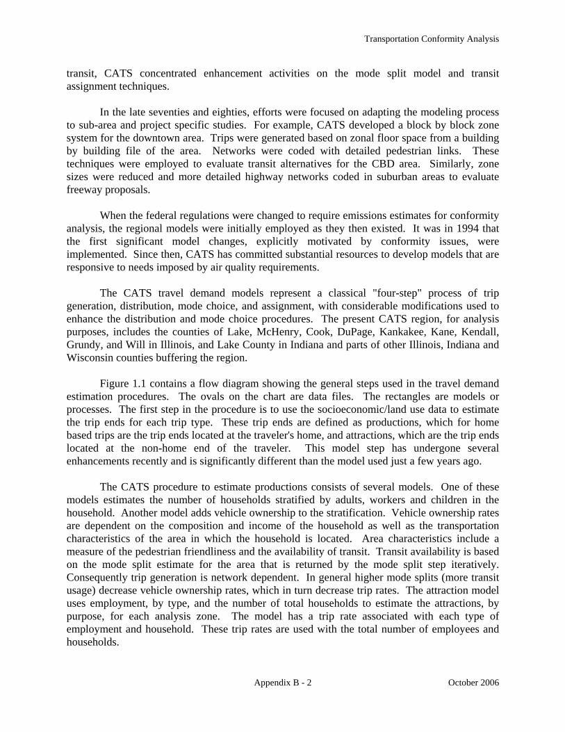
The trip ends estimated by trip generation are aggregated into analysis zones. Figure 4.1 shows the analysis zones for the CATS modeled region. These analysis zones generally follow the survey township geography. Zones are either sections (approximately one square mile) or regular subdivisions of townships (four square mile ninths of townships, nine square mile quarters of townships or whole townships). In the Chicago central area, Figure 4.2, there are 76 zones to reflect the high density of trip making in this area. Of the 76 zones, 32 are quarter-section sized zones, one-half mile by one-half mile units; while the balance of 44 are quarter-quarter-section sized zones, one quarter-mile by one quarter-mile units. Due to data availability, zones in Grundy, Kendall and Kankakee counties are based upon political townships rather than survey townships.

Transportation Conformity Analysis
Appendix B - 27 October 2006
There are 1696 analysis zones contained in the nine county Illinois study area. Sixty
more zones are in Lake County, Indiana. Twenty-two additional external zones are located along the north, west and east periphery of the region. Finally, there are twelve points of entry (POE) where major highways carrying long distance travel into, out of and through the region cross the border of the study area.
Figure 4.1 Traffic Analysis Zone System: zone95
Transportation Conformity Analysis
Appendix B - 28 October 2006
4.2 HOME BASED PERSON TRIP GENERATION
The trip generation rates were developed from the CATS 1990 Household Travel Survey1 and all household, person and trip definitions are based on the definitions used in the survey. For application of the trip generation rates, households are cross-classified by four variables: (1) number of adults; (2) number of workers; (3) vehicles available for use, and; (4) the presence or absence of children in the household.
The four variable scheme used for the cross-classification of households defines 112 different household types. Permitted values for the cross-classification variables and the resulting household types are illustrated in Table 4.1.
The following definitions apply to the above scheme for defining households. Adults include all working and nonworking members of the household of driving age, sixteen years or older. Workers are adults who indicated in the household travel survey that they were employed either full or part time. Note that six combinations of workers and adults are not permitted because there must be fewer workers than adults in the household. Children are individuals less than sixteen years of age, and by definition, a child cannot be a worker. For the purposes of defining household categories, children under the age of sixteen either are or are not present in the household. Vehicle availability is calculated as the number of autos, vans and pickups owned by the household. This definition is comparable to the one used by the census.
1 Anne C. Ghislandi, Alan R. Fijal and Ed J. Christopher. CATS 1990 Household Travel Survey: Technical
Documentation for the Household, Person and Trip Files. Working Paper 94-05, Chicago Area Transportation Study, April 1994.
Figure 4.2 Central Area Traffic Analysis Zones
6057
61 6263 64 656869 70 71 72
73 76 77
Cermak
Roosevelt
Harrison
Madison
Kinzie
Chicago
North
Sta
te
Hal
sted
Ash
land
Division
6667
54 5556 5958
74 787579 80859096
9187 8881 8382
8684
8992 93 94
959798 99 100
108 109 110
111
115
101 102 103 104 105
106 107
116
117 118
119 120
112
113 114
121
125
122 123 124
126 127 128 129

Transportation Conformity Analysis
Appendix B - 29 October 2006
Table 4.1 Household Categories Used for Trip Generation Rates
A. No Vehicles Available, Children Absent B. No Vehicles, Children Present
C. One Vehicle Available, Children Absent D. One Vehicle Available, Children Present
E. Two Vehicles Available, Children Absent F. Two Vehicles Available, Children Present
G. Three or More Vehicles Available, Children Absent
H. Three or More Vehicles Available, Children Present
Trip Definitions
Trip generation rates are estimated for workers, nonworking adults and children aged twelve to fifteen within each household category. There are, of course, no worker trip generation rates in the household cells corresponding to zero worker households. Similarly, there are not non-working adult trip generation rates in those household cells where the number of workers equals the adults in the household. Trip generation rates for children are present only for "children present" cells, households in the right half of Table 4.1.

Transportation Conformity Analysis
Appendix B - 30 October 2006
Workers' and nonworking adults' trip generation rates include both vehicle and non-motorized trips. Trip generation rates for children are vehicle trip rates, excluding school bus trips, and walking trips made by children are ignored. Trip generation rates for children are based on survey responses for children aged fourteen or fifteen, since younger children were not interviewed in the 1990 household travel survey. However, these rates are assumed applicable to all children in the twelve to fifteen age cohort.
Eleven different trip purposes are estimated, seven for workers, three for nonworking adults, and a single trip purpose for children aged twelve to fifteen. These purposes are listed in Table 4.2.
Trip purposes are defined using trip ends, which are designated with either a production or attraction trip purpose. Note, that trip productions and attractions are not the same thing as trip origins and destinations since they are independent of direction. Home trip ends are always trip productions, regardless of the direction of the trip. With the trip purposes defined in Table 4.2, work trip ends are also trip productions for work-other and work-shop purpose trips. For the remaining trip categories with the same purpose at either end of the trip (work to/from work and non-home/work to/from non-home/work purposes) the distinction between production and attraction is irrelevant. Although it may seem inconvenient to define trips in this manner, it greatly simplifies the later distribution of trips from productions to attractions.
Table 4.2 Trip Purposes Estimated
Trip Purposes Trip Maker Productions Attractions
Workers Home Work Home Shop Home Other Work Shop Work Other Work Work Non-
Home/Work Non-
Home/Work Non-Working Adults
Home Shop
Home Other Non-Home Non-Home Children (12-15 Year Olds)
Home Non-Home

Transportation Conformity Analysis
Appendix B - 31 October 2006
Trip Linking
The trip distribution model assumes that travelers are seeking out a destination from a set of potential, but not equally attractive, destinations. This model is simplistic in that it does not recognize many of the subtleties of destination choice travel behavior. One of these subtleties is that many trip purposes are often accomplished during more consequential travel for principal trip purposes. In such cases, the destination selected for the intermediate purpose is governed by the location of the primary trip destination. Another example of destination choice behavior that is difficult to model occurs when travelers make joint travel decisions, and the destination choice of one traveler is influenced by another. These problems can be partly alleviated by abstracting the trip making reported in the household travel survey to better match the uncomplicated destination choice behavior modeled in trip distribution.
For this revision of the household trip generation, home to work trips are defined so as to eliminate incidental trip purposes that take place on the way to or from work. Examples of such incidental purposes are stopping at a convenience store on the way home from work to make a minor purchase, or stopping to pick up dry cleaning. In these cases, the primary purpose of the trip is home-work and the secondary trip purpose is accomplished with only a minor route deviation or time inconvenience.
In calculating the home to work trip rates, four prerequisites had to be met before an intermediate trip purpose is considered incidental to the overall home-work trip purpose:
1. The additional time spent at the intermediate destination or destinations - the time spent inside the convenience store, for example - has to be less than thirty minutes.
2. Time in motion between home and the work place must be greater than the time
spent at the intermediate destination. If one's travel time between home and work is fifteen minutes then stopping off at the health club for an hour workout after work breaks the work trip into two distinct trips, one with a work - other purpose and a second trip with a home - other purpose.
3. The additional distance traveled to reach one or more intermediate destinations,
the excess distance between home and work, cannot be greater than five miles. 4. The distance between home and work must be greater than the excess distance
traveled to reach intermediate destinations.
In addition to this work trip linking, trips with a serve passenger or change mode purpose are linked with a subsequent trip to form a combined trip with a trip purpose suitable for trip distribution. As an example of this linking, the husband who drops his wife off at her place of work on the way to his workplace is making a home-work trip, and the serve passenger trip purpose is eliminated. Home to home trips, including those that result from the linking of serve passenger trip purposes, are also not included in the trip rates. These trips are not entirely unrepresented in the trip generation rates, however, since trips made by the passenger still are

Transportation Conformity Analysis
Appendix B - 32 October 2006
included in the rates. The vehicle trips made by children also account for some eliminated home-home trips made by their parents, such as when parents drive children to a school event and then return home without stopping for another trip purpose. Application of the Trip Rate Tables
The entire household trip generation process is sketched out in this section. Some details are omitted, particularly the trip generation associated with workers and nonworking adults residing in group quarters. The study area also extends beyond the six county region and base year and forecast socioeconomic data is required beyond that provided in the region's
socioeconomic file.
Figure 4.3 is a schematic diagram of the household trip generation process, covering the steps that convert the socioeconomic data to household trip productions and attractions. A quarter-section level trip generation input file is first developed from the regional socioeconomic file and the 1990 Census Transportation Planning Package2. Data on workers in households and household income are not in the current socioeconomic file and these household variables are obtained from the census. For future years, household worker and income data will have to be factored from the census quantities using the NIPC forecasts of households and employment.
A short program is then applied to produce a disaggregate estimate of the types of households in the quarter-section. The trip generation input file includes the total households in the quarter-section and their average quarter-section characteristics, and these need to be converted into the household types illustrated in Table 4.1. This program is the first step toward producing these household types, and it estimates quarter-section level tables of households using a three way cross-classification scheme based on the numbers of adults, workers and children in the household.
2 1990 CensusTransportation Planning Package: Urban Eliment-Parts 1, 2, and 3. Technical Documentation for
Summary Tape. Bureau of the Census, September 15, 1993.
Figure 4.3 Overview of the Household Trip Generation Process
HouseholdsCross-Classified
by Adults, Workers, Children and Income
Quartile
HouseholdVehicle
OwnershipModel
HouseholdsCross-Classified
by Adults, Workers, Children and Vehicle
Availability
Household TripGeneration Rate
Tables
Trip Productionsand Attractions
Quarter-SectionTrip Generation File
HouseholdsAve. Adults/HHAve. Workers/HHAve. Children/HHAve. Income/HH
Program to DisaggregateHouseholds
HouseholdsCross-Classified
by Adults, Workersand Children
RegionalSocioeconomic
File
1990 CensusTransportation
Planning Package
Program toMatch Workers
With Income
{

Transportation Conformity Analysis
Appendix B - 33 October 2006
The mechanics of the program feature a matrix balancing estimating procedure similar to
the one employed in the previous household trip generation procedure to disaggregate households into worker-person cells. A "seed" three dimensional matrix of observed households, or proportions of households, cross-classified by adults, workers and children is factored by the quarter-section's household attributes (average adults per household, workers per household and children per household) to create a an estimate of the quarter-section's households in each adult-worker-children cell.
The file produced by the program has one record for each quarter-section. Each of these quarter-section records contains the number of households in seventy different cross-classification cells. The seventy household types are formed by the fourteen worker-adult combinations discussed previously times five levels of children in the household (zero, one, two, three, or four plus children in the household).
A second small program further subdivides the quarter-section three-way cross-classification of households into a four-way cross tabulation by separating the households into different income quartiles. Table 4.3 lists the approximate income ranges that make up the household income quartiles.
This program also uses matrix
balancing, making use of the census two-way cross tabulation of households by workers and income levels as the seed matrix. The file produced by this program can contain up to 280 different household
cells. For most quarter-sections, however, many of the household adult-worker-children-income quartile cells contain only a fraction of a household.
The next step in the process is to apply the household vehicle ownership model.3. All of the variables needed by this vehicle ownership model are now available in either the disaggregate household file or the input trip generation file. The household vehicle ownership model produces the file for the application of the household trip generation rates. It replaces the income quartile household stratification with four levels of vehicle availability.
After application of the household vehicle ownership model, households are cross-classified in the same format as the trip generation rates. The worker, non-worker and child trip
3 Ronald W. Eash. Household Vehicle Ownership Model for 1995 TIP Conformity Evaluation. CATS Intra-Office
Memorandum, May 26, 1995.
Table 4.3 1990 Income Quartiles
Income Range Approximate Cumulative % of Census HHs
Cumulative % of
Surveyed HHsReporting
Income
<$25,000 33.2% 30.2% $25,000-$40,000
54.4% 53.4%
$40,000-$60,000
74.9% 76.1%
>$60,000 100.0% 100.0%

Transportation Conformity Analysis
Appendix B - 34 October 2006
generation rates are then multiplied by the number of individuals of each type in the cross-classified household file to produce the final estimates of trip productions and attractions.
4.3 HOUSEHOLD VEHICLE OWNERSHIP MODEL
The vehicle ownership model is a logit model similar to those used to predict mode choice behavior. There are four possible vehicle ownership levels for each household predicted by the model, either zero, one, two, or three or more vehicles per household. A vehicle is defined as an auto or a van/pickup with one ton or less cargo capacity. This definition is used in the CATS 1990 Household Survey4, and it is identical to the vehicle definition used to measure vehicle availability in the 1990 census5.
Each vehicle ownership level has an associated utility that contributes to a household's well-being. In a logit model, these utilities are linear functions of variables that describe the household and its environment. Model calibration consists of determining which variables best explain observed vehicle ownership levels and the relative importance of these variables in the utility expressions. The utilities may also include bias constants that indicate preferences toward certain levels of vehicle ownership that are not otherwise accounted for in the utility expressions.
The completed model has the following form:
Prob{Vehicle Ownership Level i} = eui
∑i
eui.
In the logit formulation, ui is the utility of household vehicle ownership level i. The model is simply that the probability of any level of vehicle ownership equals the exponential utility of that level of vehicle ownership divided by the sum of the exponential utilities for all four vehicle ownership levels.
4 Anne C. Ghislandi, Alan R. Fijal and Ed J. Christopher. CATS 1990 Household Travel Survey: Technical
Documentation for the Household, Person and Trip Files. Working Paper 94-05, Chicago Area Transportation Study, April 1994.
5 Census of Population and Housing, 1990: Summary Tape File 3 Technical Documentation. Bureau of the Census, Washington, 1991.

Transportation Conformity Analysis
Appendix B - 35 October 2006
The utility of a level of vehicle ownership is computed by the following linear equation:
ui = ∑
jαijHj + βi.
In this expression, αij is the weight attached to the j'th household variable, Hj, for vehicle ownership level i. The constant βi is the bias toward vehicle ownership level i, and it must equal zero for at least one ownership level alternative. Household Variables Used in Calibration
The selection of variables for the model calibration was driven by two hypotheses. First, larger and wealthier households should feature higher vehicle ownership levels. Second, vehicle ownership levels are reduced when the household is located in an area with reasonable alternatives to private vehicle travel. These alternatives can include non-motorized travel, pedestrian or bike modes, as well as public transportation.
The model calibration data set was built from the 1990 CATS household travel survey, census geography files and the socioeconomic data file to be used in the TIP conformity evaluation. Each record in the calibration data set is an observation for a single household in the travel survey. Households not reporting their income in the survey are excluded. The basic household characteristics - vehicle ownership, composition and income - come directly from the survey or are derived from survey data. After the household records were constructed, additional locale variables describing the quarter-section where the household is located were appended to the basic household variables.
Twelve different household variables were developed for the model calibration data set. These variables, along with brief definitions, are listed in Table 4.4 below.

Transportation Conformity Analysis
Appendix B - 36 October 2006
The workers per household and household income quartile variables are binary variables. They are defined such that additional 0,1 variables are turned on as the number of workers in a household and its income increase. For example, a household with three workers would have the three worker binary variables, WORKER1, WORKER2, and WORKER3, set equal to one. All three income variables - INCOME2, INCOME3, and INCOME4 - would be positive valued for households in the upper income quartile. These variables allow the higher ownership level
utilities to substantially increase over utilities of the lower ownership levels in wealthier households and/or households with more workers.
Workers are defined as all persons in the travel survey reported as employed, either full or part-time. Income quartiles are approximated with the income ranges used in the household travel survey. Table 4.3 shows the income ranges used for the quartiles. The table also lists the approximate percentage of regional households in the income range from the census and the corresponding proportion in the household travel survey determined from all households that reported their income.
Two other household composition variables were included in the calibration data set besides workers and income. These variables are the number of nonworking adults and the number of children in the household. For the purposes of model calibration, a nonworking adult is defined as a person of driving age, sixteen years or older, who was reported in the survey as not working full or part time. Children are defined as persons less than sixteen years of age in the household.
Two household environment variables were obtained for the calibration data set from the 1990 census. Variable AVEPEF is the average pedestrian environmental factor. The pedestrian
Table 4.4 Household Variables for Calibration Variable
Name Data
Source
Variable Description
WORKER1 Travel Survey 1 = One or More Workers 0 = No Workers
WORKER2 " 1 = Two or More Workers
0 = Less Than Two Workers
WORKER3 " 1 = Three or More Workers 0 = Less Than Three Workers
INCOME2 " 1 = Income Not in Lowest Quartile
0 = Income in Lowest Quartile
INCOME3 " 1 = Income Above Regional Average 0 = Income Below Regional Average
INCOME4 " 1 = Income in Highest Quartile
0 = Income Not in Highest Quartile
NON- WORKERS
" Nonworking Adults Sixteen Years of Age or Older
CHILDREN " Children Fifteen Years of Age or Younger
AVEPEF Census Average Pedestrian Environment for Household
AUTOMS " Average Work Trip Auto Mode Share for
Household RETAIL Socioeconomic
File Nearby Retail Employment
EMPLOYMENT " Nearby Total Employment

Transportation Conformity Analysis
Appendix B - 37 October 2006
environment of a quarter-section is measured by the number of census blocks in the quarter-section. For the model calibration data set, this quantity is averaged over the quarter-section containing the household and the quarter-sections surrounding the household's quarter-section. In most parts of the region, this means that the average pedestrian environmental factor is averaged over nine quarter-sections. The use of this variable to measure the ease with which non-motorized trips can be accomplished is discussed later.
The second census variable in the calibration data set is the average auto work trip mode share. This auto mode share is initially calculated from the census journey to work data, although in planning applications it would more likely come from the mode choice model. It is the number of workers driving, sharing a ride or taking a taxi divided by the total number of workers. This calculation is also carried out over the home quarter-section and surrounding quarter-sections. In most cases, auto trips are totaled over nine quarter-sections and divided by the workers in the same nine quarter-sections.
The final two variables are two types of employment available within walking distance of a household. These quantities were obtained from the socioeconomic file. Retail and total employment within the household's quarter-section and adjacent quarter-sections were totaled and added to the calibration data set. As before, the two employment variables are accumulated with a floating grid of quarter-sections surrounding the home quarter-section.
Calibration Results
The utility equations are, naturally enough, developed through trial and error. The software used for the calibration is the Urban Transportation Planning System program ULOGIT6. Utility expressions were first fit using only the binary variables for workers in a household. After estimating the household worker coefficients that provided the best possible fit without other variables, the binary variables for income were moved into the utility expressions. The remaining household variables were then shuffled in and out of the equations, retaining only the ones that improved the model's calibration.
Model calibration results are tabulated in Table 4.5. The calibration was initially carried out using one-half the data set. After selection of the variables in the utility expression, the calibration was repeated with the unused observations. No major differences in coefficient values where found when the two calibrations were compared. The results reported in Table 4.5 use all 15,340 unweighted household observations.
The utility expressions are defined so that zero vehicle ownership does not have a utility. The household variables CHILDREN, RETAIL and EMPLOYMENT were dropped during the model calibration process because they did not significantly contribute to the utility of any vehicle ownership level. Both employment variables, RETAIL and EMPLOYMENT, are quite
6 ULOGIT: Logit Calibration Program. Urban Transportation Planning System. Urban Mass
Transportation Administration/Federal Highway Administration, U.S. Department of Transportation, Washington, DC, March 1982.

Transportation Conformity Analysis
Appendix B - 38 October 2006
correlated with the other two household environment variables AUTOMS and AVEPEF. The standard errors of the coefficient and the T-statistics at the bottom of Table 4.5 indicate that all coefficients, except for the bias associated with single vehicle ownership, are significantly different from zero.
Table 4.5 Household Vehicle Ownership Model Calibration Results
A. Calibration Coefficients
Household Variables Vehicle
Ownership
WORKER1
WORKER2
WORKER3 NON-
WORKERS
INCOME2
INCOME3
INCOME4
AUTOMS
AVEPEF Unadjusted
Bias
0 1 0.763 1.158 2.718 -0.080 0.3252 3.408 2.927 2.039 2.124 0.760 5.623 -0.132 -6.683
3+ 5.329 4.322 2.638 3.173 2.124 0.760 0.481 5.623 -0.179 -11.383
B. Standard Error of Coefficient
Household Variables
Vehicle Ownership
WORKER1
WORKER2
WORKER3
NON-WORKERS
INCOME2
INCOME3
INCOME4
AUTOMS
AVEPEF
Unadjusted Bias
0 1 0.093 0.096 0.286 0.006 0.316 2 0.134 0.068 0.059 0.114 0.059 0.355 0.007 0.275
3+ 0.226 0.103 0.073 0.074 0.114 0.059 0.054 0.355 0.008 0.339
C. Coefficient T-Statistic
Household Variables Vehicle
Ownership
WORKER1
WORKER2
WORKER3 NON-
WORKERS
INCOME2
INCOME3
INCOME4
AUTOMS
AVEPEF Unadjusted
Bias
0 1 8.21 12.10 9.49 -13.62 1.03 2 25.53 43.00 34.60 18.62 12.97 15.83 -19.89 -25.49
3+ 23.59 42.15 36.09 43.15 18.62 12.97 8.86 15.83 -23.73 -34.59
The signs of the variable coefficients seem appropriate. All model coefficients, except
for the AVEPEF coefficient, have positive signs. Most would agree that additional workers, nonworkers and income in a household logically should add to the utility of greater vehicle ownership. It also seems reasonable that each added worker and each added quartile of income adds less to the utility of vehicle ownership than prior workers and income. The positive relationship between auto work trip mode share and vehicle ownership appears correct. An improved pedestrian environment, however, almost surely reduces vehicle ownership levels, which is consistent with the negative sign on the AVEPEF coefficient.
Additional measures of how well the model fits the observed data are provided in Table
4.6. These are the standard goodness of fit statistical measures provided by the ULOGIT

Transportation Conformity Analysis
Appendix B - 39 October 2006
program. In order to evaluate them, one must first generally understand how the logit equation is fit to the observed data using the maximum likelihood procedure.
The likelihood of some sequence of events occurring is the probability of event one taking place times the probability of event two occurring, and so forth, until the end of the sequence of events is reached. For the households in the calibration data set, each of these probabilities is the probability determined by the model that the household owns the number of vehicles it actually owns, as shown below:
Likelihood = ∏k=1
15340ηk
i∗Pki .
In this equation, Pki is the probability given by the model that household k has vehicle ownership
level i, while ηki is a binary 0,1 variable that is one when the actual vehicle ownership of
household k is equal to i. To simplify the calculations, the natural log of the likelihood is usually maximized rather
than the likelihood itself, as follows:
Ln{Likelihood} = . In a perfect model, the probability of a particular household vehicle ownership level would be one for the actual number of vehicles owned by the household and zero otherwise. The maximum Ln{Likelihood} is, therefore, zero. All calibrated, but imperfect, models have a negative Ln{Likelihood}. The first measure of the model's quality listed in Table 4.6 is a hypothesis test that the calibrated model is not significantly better than a simple equal probability model of household vehicle ownership. The null hypothesis is that each household has an equal probability (0.25) of being in one of the four levels of vehicle ownership. A second similar hypothesis test is also evaluated in ULOGIT for a proportional model of household vehicle ownership. The null hypothesis is that the probabilities of vehicle ownership are proportional to their appearance in the calibration data set. These proportions are approximately 0.06, 0.31, 0.46 and 0.17 for zero, one, two and three plus vehicles owned, respectively. Both null hypotheses are easily rejected, since the calibrated model is far superior to either the equal or proportional probability models.
The final measure in Table 4.6 is termed the pseudo R-square, a statistic that varies between zero and one in much the same way that the R-square statistic varies in least squares regression. There is no other similarity, however. The pseudo R-square measures the quality of
Table 4.6 Model Calibration Statistics
Statistical Measure Value Test of Equal Probability
(Chi Square, 20 Degrees of Freedom)
19,960
Test of Proportional Probability
(Chi Square, 17 Degrees of Freedom)
13,800
Pseudo R-Square 0.469

Transportation Conformity Analysis
Appendix B - 40 October 2006
the calibrated model relative to the equal probability and perfect - zero Ln{Likelihood} - models. In this example, the calibrated model is approximately halfway between an equal probability model and a perfect fit to the data.
Bias Constant Adjustment
The calibration data set contains slightly different proportions of households at the four vehicle ownerships than the census. There are too few zero and one vehicle households and too many households with two or more vehicles. This bias is corrected by adjusting the bias
coefficients to slightly increase the zero and one vehicle ownership probabilities. Final bias coefficients are listed in Table 4.7.
Table 4.7 Final Household Vehicle Ownership Bias
Vehicle
OwnershipOriginal
Bias Adjusted
Bias 0 0.000 0.000 1 0.325 -0.656 2 -6.683 -8.114
3+ -11.383 -12.825

Transportation Conformity Analysis
Appendix B - 41 October 2006
Pedestrian Environmental Factor and Mode Share
Vehicle ownership does not totally depend on the composition of the household and its income, but also upon external factors that affect vehicle usage. For example, vehicle ownership generally increases for high income households, yet there are a sizable number of very wealthy households on Chicago's north side with low vehicle ownership levels. The household vehicle ownership model had to recognize that some households are able to substitute pedestrian, bike and transit travel for private vehicle travel, which reduces their need to own private vehicles.
Average automobile work trip mode share is an obvious location variable that helps indicate whether a private vehicle is necessary for work travel. In calibrating the model, this variable was developed from the 1990 census journey to work data. However, when this vehicle ownership model is used in a typical planning application, mode choice is estimated by subsequent models. How can an end product from the use of these sequential models be available as an input for one of the earliest models in the sequence?
While there is a question of comparability between the census auto mode share used for calibration and modeled mode share, the only solution is to iterate back through the household vehicle ownership model when the estimated auto mode share changes substantially from the base, as might be the case when major transit facilities are planned or when a major shift in the cost of using a mode is anticipated. Note that the auto mode share used for model calibration reflects workers who work at home or workers who commute by non-motorized modes. Auto mode share is here defined as auto work trips divided by all workers, and it is not exactly the auto mode choice produced by the model, which only deals with vehicle trips.
Figure 4.4 shows the average auto mode share variable used for model calibration for the six county northeastern Illinois region. The grayscale is reversed so that the lowest auto work trip mode shares have the darkest shading. The scattered low auto work trip mode share quarter-sections in the outlying collar counties seem incongruous, but they correspond to quarter-section where farming is the principal occupation, or where there are no workers and the variable is arbitrarily set to zero.

Transportation Conformity Analysis
Appendix B - 42 October 2006
The average pedestrian environmental factor (PEF) shown in Figure 4.5 is a surrogate variable in the model that takes the place of an actual survey of pedestrian and bicycle facilities. It is defined as the number of census blocks in a quarter-section. Census blocks are closed geographic areas that are generally formed from streets. They are not necessarily rectangular or always contiguous with city blocks due to alleys and cul-de-sacs. A greater density of census blocks implies a more regular street network and more local streets, both of which improve walking and biking conditions.
Highest PEFs are located in the most dense part of the central area. A half city block street grid (one-sixteenth of a mile) would produce a maximum PEF of sixty-four. A dense city neighborhood with streets in a one-eighth by one-sixteenth mile pattern has a PEF of thirty-two. Established suburban areas feature PEFs on the order of ten to twenty. PEFs for newer suburban areas without regular street patterns may be five or less. The average PEFs in Figure 4.5 are also averaged over adjacent quarter-sections.
Since the pedestrian environmental factor is taken from the census, it must be computed for future planning applications when census data is not available. This is done by analogy to existing development. In other words, applying the current PEFs for existing development forward in time to areas forecasted to develop in a manner similar to existing areas. The PEF
Figure 4.4 Work Trip Auto Mode Share Figure 4.5 Pedestrian Environmental Factors
AutoMode Share
0.0 - 0.2 0.2 - 0.40.4 - 0.60.6 - 0.80.8 - 1.0
PedestrianEnvironmental Factor
0-88-16 16-24 24-32 32-40 40-48 48-56

Transportation Conformity Analysis
Appendix B - 43 October 2006
variable also provides another means of generating development scenarios that impact travel behavior. One could hypothesize a scenario with future residential development reverting back to more traditional forms than the auto oriented suburban residential development that has taken place over the past four decades. Quarter-sections undergoing development in the forecast would be assigned PEFs more typical of regular urban residential blocks than recently developed residential subdivisions. Model Behavior
Figure 4.6 illustrates the behavior of the model for six typical households. These households feature different numbers of workers and nonworking adults and income levels. The distinction between urban and rural is created by alternate pedestrian environmental factors and auto mode shares. The urban household vehicle ownership examples assume an auto work trip mode share of forty percent and a PEF of twenty-five. Suburban households are located in areas with a ninety percent auto mode share and a PEF of five.
The model results shown in Figure 4.6 appear intuitively correct. Higher vehicle ownership levels are associated with the larger and higher employment typical households. The urban and suburban households also show markedly different vehicle ownership level probabilities.

Transportation Conformity Analysis
Appendix B - 44 October 2006
Figure 4.6 Predicted Vehicle Ownership for Typical Households A. No Workers, Low Income B. One Worker, Low Income
0.00
0.20
0.40
0.60
0.80
1.00
Pro
babi
lity
Urban SuburbanLocation
0 Cars
1 Car
2 Cars
3+ Cars
0.00
0.20
0.40
0.60
0.80
1.00
Pro
babi
lity
Urban SuburbanLocation
0 Cars
1 Car
2 Cars
3+ Cars
C. One Worker, One NonWorker, Average Income
D. Two Workers, Average Income
0.00
0.20
0.40
0.60
0.80
1.00
Pro
babi
lity
Urban SuburbanLocation
0 Cars
1 Car
2 Cars
3+ Cars
0.00
0.20
0.40
0.60
0.80
1.00
Pro
babi
lity
Urban SuburbanLocation
0 Cars
1 Car
2 Cars
3+ Cars
E. Two Workers, High Income
F. Two Workers, One NonWorker, High Income
0.00
0.20
0.40
0.60
0.80
1.00
Pro
babi
lity
Urban SuburbanLocation
0 Cars
1 Car
2 Cars
3+ Cars
0.00
0.20
0.40
0.60
0.80
1.00
Pro
babi
lity
Urban SuburbanLocation
0 Cars
1 Car
2 Cars
3+ Cars

Transportation Conformity Analysis
Appendix B - 45 October 2006
4.4 ALLOCATION OF NON-HOME LOCATION PRODUCTIONS/ATTRACTIONS
All home based trips are accounted for after the trip production and attraction calculations described in the previous section. However, we only know the location of the home trip productions. The locations of all other trip productions and attractions are unknown at this point.
Non-home productions
and attractions are allocated to zones by four regression equations for: (1) home to work attractions; (2) home to other attractions; (3) non-home to non-home attractions and productions at work sites; and (4) non-home to non-home trip attractions and productions not at work. These four regressions were calculated with zone trip productions and attractions from the 1990 Household Travel Survey as the dependent variables and zone employment and households from the socioeconomic file as independent variables.
Non-home trip productions and attractions are allocated proportionally to zones using the
regression estimates as weights for the zones. Note that the total number of non-home trip productions and attractions is still equal to the totals established by the home based trip generation calculations. As shown in Table 4.8, no distinction is made between employee and non-employee trip ends for this allocation.
Table 4.9 summarizes the results of these regressions. Variables used in the regression equations are listed across the top of the table. These are seven different types of employment and the households contained within each zone in the socioeconomic file. As might be expected, the household variable shows up only in the regression equations for attractions to non-work trip ends. The regressions are constrained so that no productions or attractions are allocated to a zone that does not have employment or households.
Table 4.8 Zone Allocations of Home Based Trip Ends
Trip Purpose Productions Attractions
Employee Home to Work Home Zone Regression for Home to
Work Attractions Home to Other Home Zone Regression for Home to
Other Attractions Non-Home to Non-Home (Located at Work Site)
Regression for Non-Home to Non-Home Work
Productions/Attractions
Regression for Non-Home to Non-Home Work
Productions/Attractions Non-Home to Non-Home (Not Located at Work Site)
Regression for Non-Home to Non-Home Non-Work Productions/Attractions
Regression for Non-Home to Non-Home Non-Work Productions/Attractions
Non-Employee
Home to Other Home Zone Regression for Home to Other Attractions
Non-Home to Non-Home (Not Located at Work Site)
Regression for Non-Home to Non-Home Non-Work Productions/Attractions
Regression for Non-Home to Non-Home Non-Work Productions/Attractions

Transportation Conformity Analysis
Appendix B - 46 October 2006
Trip generation for persons living in group quarters rather than in households is next
added to the household trip generation. In most cases, the non-worker single person household trip generation rate is used for these individuals. As a precaution, zones with large numbers of persons in group quarters were examined individually to determine whether this rate was appropriate. The most important objectives of this zone by zone evaluation were to eliminate incarcerated persons from the trip generation and to estimate reasonable trip generation figures in the zones containing Great Lakes Naval Training Base and Fort Sheridan.
Table 4.9 Summary of Trip Generation Equations for Allocation of Non-Home Located Productions and Attractions
Variables in Model
Allocation Model
Manufact. Employment
Service
Employment
Local Retail
Employment
Regional Retail
Employment
T.C.U.W.
Employment
Government Employment
Other
Employment
Households
Regression Adjusted
R-Squared Home to Work Attractions
0.779
Parameter 0.466 0.703 2.408 1.092 0.481 1.262 2.974 Standard Errors 0.082 0.052 0.138 0.160 0.111 0.086 0.396 T for H0 that Parameter = 0
5.69 13.59 17.39 6.84 4.33 14.69 7.51
Home to Non-Work Attractions
0.663
Parameter 0.251 3.558 4.008 1.489 1.121 0.968 Standard Errors 0.092 0.278 0.298 0.160 0.493 0.051 T for H0 that Parameter = 0
2.71 12.80 13.43 9.32 2.27 19.08
Non-Home to Non-Home Work Attractions
0.679
Parameter 0.044 0.081 0.343 0.105 0.089 0.505 Standard Errors 0.014 0.008 0.023 0.025 0.014 0.059 T for H0 that Parameter = 0
3.10 9.87 15.17 4.10 6.43 8.59
Non-Home to Non-Home Non-Work Attractions
0.680
Parameter 0.915 0.922 0.143 0.356 0.182 Standard Errors 0.055 0.058 0.032 0.092 0.010 T for H0 that Parameter = 0
16.55 15.79 4.53 3.85 17.80

Transportation Conformity Analysis
Appendix B - 47 October 2006
4.5 TRUCK TRIPS
The following briefly describes the method used to estimate truck trip generation and distribution. The objective was to use the truck trip generation and distribution relationships established for previous truck modeling and make them responsive to the new horizon year and alternative land use scenarios. 1990 truck productions and attractions were regressed against 1990 socioeconomic variables with the following result:
Table 4.10 Truck Trip Regression Households Manufacturing
Emp Retail Emp
Trans. Comm. Utility Emp
R-Square
B-trucks attractions 0.187041 0.320939 0.394569 0.225288 0.8442 B-trucks productions 0.181715 0.320220 0.394766 0.216512 0.8446 L-trucks attractions 0.049859 0.102433 0.164578 0.076859 0.8410 L-trucks productions 0.047472 0.101758 0.163254 0.072359 0.8402 M-trucks attractions 0.012200 0.063089 0.081374 0.042461 0.8537 M-trucks productions 0.011872 0.062684 0.080829 0.040578 0.8532 Heavy attractions n/a 0.075066 0.034920 0.049806 0.7790 Heavy productions n/a 0.074602 0.034937 0.049984 0.7797
The 1990 triptable totals were used as the “working population” (i.e. a regional control total of truck trips) with the accumulated regression error reapplied as a uniform factor across the region. The 1990 estimated productions and attractions were then distributed using a gravity model with impedance calibrated using previously prepared 1990 truck triptables and 1990 base highway times.
The 1990 socioeconomic coefficients were then applied to the socioeconomic data for each analysis year in order to forecast productions and attractions under each land use scenario. The accumulated regression error was applied as a uniform factor across the region with the total trips also corrected to a new “working population” estimated by interpolating or extrapolating the previously estimated growth in total truck trips to each analysis year. The productions and attractions were then distributed as described above but with impedances taken from the appropriate test highway network. As noted above, in the current analysis, the truck triptables have been re-balanced based on correlation with updated socioeconomic data.

Transportation Conformity Analysis
Appendix B - 48 October 2006
5 TRIP DISTRIBUTION The trip distribution model connects trip productions and attractions. It takes the zone trip productions and attractions produced by the trip generation model and converts them into movements between zones, or trip tables. In the iterative portion of the modeling process, the intervening opportunity trip distribution model is used to distribute person trips using a composite impedance from both the highway and transit networks. In this process, trip distribution is performed after trip generation and before mode choice, estimating the destination choices of person trips regardless of mode. The resulting person trip tables are then input to the mode choice model. The intervening opportunity model is also used to distribute commercial vehicle (truck) trips and, in the final step, automobile vehicle trips using highway only impedances.
5.1 AN OVERVIEW OF THE INTERVENING OPPORTUNITY MODEL
The intervening opportunity model of trip distribution was originally formulated in the late 1950s. It is based on two simple premises. First, travelers try to minimize travel time and cost, and secondly, there is some constant probability that a traveler will find a potential destination acceptable. To illustrate, a person making a shopping trip does not always stop at the nearest store, they first consider whether the nearest store is acceptable or not, if not, move on to the next closest store, and so on, until an acceptable destination is found.
These premises can be restated in terms of the analysis zones and trip attractions and trip productions that are built into the model as follows. The probability that a trip production will end in a particular destination zone is the product of two probabilities, the probability that the trip has not already terminated nearer the origin zone times the probability that an acceptable attraction exits in the destination zone.
Mathematically, this probability can be expressed as:
( ) ALPP ∆−=∆ **1
Where P equals the probability that the trip is completed before the destination zone is reached; ∆P is the marginal probability of completing the trip due to the added attractions (∆A) of the destination zone. Finally, L is the constant probability of stopping at any single attraction.
Applying this simple model raises a number of complex questions. What is meant by
nearest zone and in what sequence are attractions considered by the traveler? Is proximity determined by the shortest travel time or least cost mode or route, or by some measure that reflects the alternative modes and routes available between origin and destination zones? Even more fundamental model questions are associated with the L-values, including how travel and tripmaker characteristics affect these quantities, and how they change over time?

Transportation Conformity Analysis
Appendix B - 49 October 2006
The balance of this section discusses how the intervening opportunity trip distribution model was applied by CATS in the air quality conformity TIP and RTP network evaluations. The major change introduced into the model from previous applications is the use of a combined measure of transit and highway cost to rank zones in order of increasing cost from the origin zone.
The model was calibrated to data from the recent CATS household survey. The following sections discuss how the L-values are calibrated and then smoothed into a monotonic function of accessible attractions. This function is used to estimate future L-values. Regression relationships were developed to estimate L-values as a function of the attractions that are reachable within a particular combined transit-highway cost from the origin zone. This approach to L-value calibration allows the cost and time characteristics of the highway and transit networks, as well as trip productions and attractions, to influence the trip distribution.
5.2 THE DOUBLY CONSTRAINED INTERVENING OPPORTUNITY MODEL
The intervening opportunity trip distribution model is a member of the gravity model family of trip distribution models. After some algebra, the above relationship indicates that trips between zones are proportional to the trip productions in the origin zone and attractions at the destination zone, and inversely proportional to the difficulty of traveling between the two zones. This is the well-known general formulation of the gravity model. In most gravity models, the difficulty of traveling between zones, the impedance faced by the traveler, is related to the travel time or travel cost between zones. However in the intervening opportunity model, impedance also is a function of the attractions, or intervening opportunities, the traveler encounters while journeying between zone pairs.
The doubly constrained intervening opportunity model consists of four sets of equations shown below. To solve these equations, travel impedance is first determined, then the remaining three sets of equations are simultaneously solved using an iterative matrix balancing algorithm:

Transportation Conformity Analysis
Appendix B - 50 October 2006
1. F
Tij
jiij
βα= , for all i, j zone pairs.
2. , e VLF ijiij = for all i, j zone pairs.
3.
∑=
j ij
j
ii
F
Pβα , for all origin zone i.
4. ∑
=
i ij
i
ij
F
Aα
β , for all destination zone j
In the above equations, Tij stands for person trips distributed from zone i to zone j. The αi and βj are balancing coefficients for zone i and zone j, Pi and Aj are the trip productions for zone i and trip attractions for zone j, and lastly, Fij is the impedance between zones.
The equations are the actual trip distribution model that links together trip productions and attractions. Zone trip productions and attractions produced by the trip generation model are converted into movements between zones, or trip tables. There is one distribution equation for every origin zone-destination zone pair.
In the doubly constrained version of the intervening opportunity model, two sets of equations restrict the total trips distributed from an origin zone to the zone's trip productions, and the total trips received by a destination zone to the zone's trip attractions. These are the third and fourth sets of above equations. These equations ensure that the row sums of the trip table equal trip productions, and the trip table's column sums equal trip attractions. There is one production constraint equation for each origin zone and one attraction constraint equation for every destination zone.
The second equation in the model defines the impedance functions, Fij in the intervening
opportunity model equals eLiVij. The form of these functions is exponential, with an exponent that includes the bypassed opportunities, Vij, and the previously discussed L-value parameter for the origin zone, Li. The Vij term equals the number of attractions that are closer to the origin zone than the destination zone (the destination zone's attractions are excluded from these subtended attractions). Note that impedance increases with higher L-values and increasing opportunities. An impedance value is determined for all zone pairs.
To gain some sense of the magnitude of the calculations required for trip distribution, consider that there are nearly 5,400,000 equations in the above model that need to be solved. This figure is for the 1640 analysis zones used in 1993-1994 conformity evaluations. The model

Transportation Conformity Analysis
Appendix B - 51 October 2006
is also applied separately for three trip types, home productions to work attractions, home productions to non-work attractions and non-home productions to non-home attractions.
5.3 MODEL CALIBRATION
Travel time and cost are not explicitly measured in the Fijs, but one way they enter the model is through the ranking of trip attractions from the origin zone. In the conformity model runs, a generalized cost of travel across modes is used for ranking zones. This generalized cost reflects the cost and time of travel by both transit and auto. It is calculated by the mode choice model used by CATS. Generalized cost also plays an important role in calibration of the trip distribution model, as discussed in the following sections.
Calibration of any trip distribution model usually means fitting the model's average trip lengths, or trip length distribution, to observed trip characteristics. The CATS trip distribution model is calibrated to average trip lengths for outbound trips from subareas in the region, and to the average trip length for trips received by the central area. In the calibration process, the L-values primarily control the trip lengths for trips sent, while the generalized cost quantity is used to regulate the length of trips received by the central area.
The trip distribution model calibration, therefore, has two stages. L-values are calibrated to average sent trip lengths, and then the relative importance of transit and highway modes in the distribution generalized cost is calibrated from the trip lengths of trips received by the central area. In all the calibration calculations, the trips referred to are person trips in vehicles. The calibration calculations are also repeated for the three trip purposes.

Transportation Conformity Analysis
Appendix B - 52 October 2006
This approach to trip distribution model calibration proceeds in the following manner:
1. Base year 1990 L-values were calibrated for fifteen subareas in the region. These L-values were estimated by matching model trip lengths to observed trip lengths from the household travel survey. L-values were repeatedly changed until the desired model trip lengths were obtained. Lower L-values produce longer average trip lengths and higher L-values result in shorter trip lengths.
2. Additional bias in favor of transit was added to the generalized cost until the
average length of trips received by the Chicago central area roughly equaled the observed trip length in the 1990 household travel survey. Adding this bias toward transit reduces the cost of travel between zone pairs served by transit compared to zone pairs only served by auto. This substantially increases the accessibility of the central area compared to other destinations. The central area becomes a more attractive destination for longer distance trips located along the radial commuter rail and rail transit lines serving the central area.
3. Base year 1990 L-values for the fifteen subareas were readjusted so that
model trip lengths matched observed trip lengths with the transit bias. The transit bias was then fine tuned to restore the trip length distribution for trips to the central area. This procedure was repeated until a reasonable fit was obtained for both subarea sent and central area received trip lengths.
5.4 GENERALIZED HIGHWAY-TRANSIT COST ESTIMATION
The CATS mode choice model simulates individual person trip mode choice behavior, first estimating the costs and times of making the trip by transit, and then the probability of choosing each mode based on these alternative trip characteristics. Line-haul costs and times for travel by transit and auto are determined by the paths between zones, but the costs and times required to reach or depart line-haul facilities are simulated through submodels, which include central area parking and access to a rail station. These simulated and line-haul costs and times are independent variables in the multinomial logit function that predicts the probability that one or the other mode will be selected. Once this probability is determined a trip is allocated to transit or auto modes using Monte Carlo simulation. All person trips are individually simulated during mode choice, nearly twenty million trips counting all trip purposes.
The cost calculation part of the CATS mode choice model is used before trip distribution to estimate the multi-mode generalized travel cost. When the model is applied prior to distribution, five person trips are simulated for each trip interchange between zones. The transit and highway costs and times for these five trips are then estimated in the same manner as in mode choice, but mode choice calculations are not done. The interchange's transit and highway cost is then averaged from the five simulated trips' characteristics.

Transportation Conformity Analysis
Appendix B - 53 October 2006
The values estimated by the mode choice model are the weighted sums of the cost and time variables used in the mode choice model's multinomial logit function. This logit model has the following form:
ee
eP
ii
transiti
ii
autoi
ii
autoi
autoVV
V
τωω
ω
+−−
−
∑+∑
∑=
In the above mode choice equation, Pauto is the probability that the person trip is by
auto. The Viauto
and Vitransit
are cost and time mode choice variables for completing the trip by auto or transit, and the ω i s are the weights associated with each cost and time variable. Costs are in cents and measured in 1970 dollars, and times are in minutes.
Variables in the model and their weights in the linear multinomial cost expression are listed in Table 5.1. The exponents in the logit mode choice function are negatively signed because the cost and time quantities in the model have negative utilities. These cost and time quantities are multiplied by the positive ω i s listed in Table 5.1 to be consistent with the negative sign on the exponent. A more negative exponent, which equals a larger ∑
ii iVω , means a lower
probability of choice. A mode that has high relative times and costs is an unlikely choice.

Transportation Conformity Analysis
Appendix B - 54 October 2006
The τ quantity is the bias for or against transit. A negative τ indicates a bias toward auto away from transit. If the costs and travel times of the two modes are equal and the τ value is negative, then there will be less than a fifty percent probability that transit will be chosen. A positive τ indicates a greater than fifty percent chance of selecting transit.
The mode choice model actually
estimates ∑i
iautoiVω and τω +∑
ii
transitiV for each
zone pair. Some additional manipulations are necessary to obtain the generalized cost across modes, which is defined as the negative log sum of the logit function's denominator. It is calculated from these two sums as follows:
⎭⎬⎫
⎩⎨⎧ ∑+∑−= +−− ee i
itransiti
ii
autoi
transitauto VVLnC τωω/
This multi-mode generalized cost can
also be interpreted as the cost belonging to some abstract mode whose service characteristics are equivalent to those of a joint transit-highway alternative. Calculation of the generalized cost from the values provided by the mode choice model is accomplished in a separate step that determines the log sum.
5.5 CALIBRATED L-VALUES
To start the calibration process average person trip lengths were tabulated from the household travel survey for trips from thirteen subareas: (1) Chicago; (2) the North Shore, Northwest, North Central, Central, Southwest and South Cook County regions, and; (3) the DuPage, Kane, Kendall, Lake, McHenry and Will collar counties. Calibration average trip lengths for two additional subareas, Grundy County and Lake County, Indiana, were estimated from trip lengths in adjacent counties and average travel times reported in the 1990 census journey to work data.
During the calibration of the trip distribution, trip lengths for person trips to the central area were too short when the model was only calibrated to sent trip lengths from the subareas.
Table 5.1 Mode Choice Parameters
Mode Choice Variable (Vi) Weight (wi )
Home to CBD Work Trips Auto and Transit In-Vehicle Time 0.0159 Auto and Transit Cost 0.0085 Auto and Transit Excess Time for Access/Egress
0.0468
Transit Bias (b) -0.6059 Transit Out-of-Vehicle Time 0.0290 Transit First Headway 0.0173 Home to Non-CBD Work Trips Auto and Transit In-Vehicle Time 0.0186 Auto and Transit Cost 0.0072 Auto and Transit Excess Time for Access/Egress
0.0584
Transit Bias (b) -0.4983 Transit Out-of-Vehicle Time 0.0399 Transit First Headway 0.0811 Home to Other Trips Auto and Transit In-Vehicle Time 0.0114 Auto and Transit Cost 0.0329 Auto and Transit Excess Time for Access/Egress
0.0663
Transit Bias (b) -0.2726 Transit Out-of-Vehicle Time 0.0589 Transit First Headway 0.0610 Non-Home to Non-Home Trips Auto and Transit In-Vehicle Time 0.0114 Auto and Transit Cost 0.0329 Auto and Transit Excess Time for Access/Egress
0.0663
Transit Bias (b) -0.8072 Transit Out-of-Vehicle Time 0.0589 Transit First Headway 0.0610

Transportation Conformity Analysis
Appendix B - 55 October 2006
For the purposes of the trip distribution calibration, the central area is defined as the zones shown in Figure 5.1. The solution to this problem was to increase highway costs and decrease transit costs. In the distribution model, this affects the ranking of zones to increasingly favor zone pairs with competitive transit service. Zone pairs with transit service become closer relative to zone pairs without transit service. This is particularly important for the central area, which is well served by radial transit lines. Trip productions located along these radial lines are increasingly drawn to central area attractions as transit costs decrease relative to auto.
Table 5.2 shows the costs added and subtracted
from the mode choice model's estimated highway and transit costs. This adjustment is made before the negative log sum is taken. The values in Table 5.2 are in the same dimensionless units as the mode choice model's weighted sums of costs and times. Note that transit and highway costs can be scaled by a constant without changing the mode choice probabilities. This means that the absolute value of the costs and the additional bias favoring transit cannot be determined.
The only significant cost is the relative cost difference between using the two modes. After these additions and subtractions, the combined transit-highway generalized cost roughly ranges between 4.0 and 12.0 cost units. The two non-work trip purposes have slightly higher costs than work purpose trips.
Two other minor adjustments were made in the cost calculations to improve the distribution. First, the combined transit-highway cost (after the log sum is taken) was increased by 0.3 for all trip interchanges across the Illinois-Indiana state line for all trip purposes, regardless of direction. This was done to reduce the number of interchanges across the state line to match observed data. It can be argued that the state line is an additional barrier to movement
that cannot be correctly represented in the Fij impedance.
The second minor adjustment
was caused by the way the CATS' transit network is coded. Trips between adjacent zones often can travel through walk links without boarding a transit line. For these short trips, the transit cost is computed assuming a walking speed of twenty minutes per mile, the
Figure 5.1 Central Area Zones Distribution Calibration
6057
61 6263 64 656869 70 71 72
73 76 77
Cermak
Roosevelt
Harrison
Madison
Kinzie
Chicago
North
Sta
te
Hal
sted
Ash
land
Division
6667
54 5556 5958
74 787579 80859096
9187 8881 8382
8684
8992 93 94
959798 99 100
108 109 110
111
115
101 102 103 104 105
106 107
116
117 118
119 120
112
113 114
121
125
122 123 124
126 127 128 129
Table 5.2 Transit and Highway Bias Adjustment for Trip Distribution
Trip Purpose Transit Cost Reduction
Auto Cost Increase
Home Production to Work Attractions
-1.0 +1.1
Home Productions to Non-Work Attractions
-1.0 +2.0
Non-Home Productions to Non-Home Attractions
-1.0 +2.0

Transportation Conformity Analysis
Appendix B - 56 October 2006
transit out-of-vehicle time coefficient and the transit bias. All of these changes in the mode choice cost values take place outside of the mode choice model and apply only to the combined transit-highway cost used for trip distribution.
Table 5.3 summarizes the results of the person trip distribution calibration. It lists the average trip lengths from the household travel survey, the comparable trip length from the trip distribution and the L-value calibration coefficient for the subarea. The subareas in Cook County are approximately the same as the Regional Councils.
Table 5.3 1990 Calibrated Person Trip Lengths and L-Values
Home to Work Home to Other Non-Home to Non-Home
Subarea Survey
Trip Length (miles)
Calibrated Trip
Length (miles)
CalibratedL-Values
(10-6)
Survey Trip
Length (miles)
CalibratedTrip
Length (miles)
CalibratedL-Values
(10-6)
Survey Trip
Length (miles)
CalibratedTrip
Length (miles)
CalibratedL-Values
(10-6)
Chicago 8.6 9.0 1.30 4.8 5.3 2.23 5.8 6.1 2.57 Cook North Shore 10.3 10.4 1.40 4.7 4.6 4.07 5.6 5.7 5.21 Northwest 10.7 10.4 1.79 5.2 5.3 5.36 5.8 5.8 6.32 N. Central 8.5 8.7 1.55 4.7 4.7 3.61 5.8 5.8 4.06 Central 9.2 9.5 1.49 4.3 4.6 6.59 4.7 5.0 7.71 Southwest 11.8 11.7 1.88 4.5 4.7 7.23 4.8 5.0 9.65 South 13.5 13.4 3.01 5.3 6.0 9.67 5.5 5.7 11.34 DuPage 12.0 11.2 1.66 4.6 4.7 8.97 5.9 5.6 7.24 Kane 12.3 11.3 5.95 6.0 5.9 13.61 4.9 5.3 25.42 Kendall 11.7 11.1 18.29 5.2 5.2 73.54 5.5 5.6 67.58 Lake 13.2 12.1 4.59 5.7 5.9 17.72 6.5 6.5 15.47 McHenry 15.2 14.3 10.15 5.8 5.9 46.77 5.2 5.7 59.01 Will 14.7 13.1 5.43 6.2 6.2 18.91 6.1 6.6 28.94 Grundy 10.7 76.03 5.2 133.30 6.0 245.64 Lake, Indiana 10.1 9.77 3.8 18.91 4.9 28.94 To CBD 14.9 14.4 11.3 8.7 7.7 5.4 Region 10.7 10.6 5.0 5.3 5.7 5.9
5.6 FORECASTING L-VALUES
After calibrating the L-values to existing data, the next question to be asked is what are future L-values? The simplest assumption is to argue that these quantities should remain constant into the future. This assumption generally causes trip lengths to shorten as trip attraction opportunities increase over time. Future travelers encounter more opportunities to complete their trip as they travel from the origin zone due to additional development. If the probability of selecting a destination does not change over time, they will find an acceptable destination closer to the origin. The problem with this argument is that average trip lengths have historically not declined in spite of increased development.

Transportation Conformity Analysis
Appendix B - 57 October 2006
The plot in Figure 5.2 is a first step toward understanding how L-values change with development. It compares the home to work trip L-values in Table 5.3 with the density of work attractions in each subarea. This plot shows that the relationship between L-values and density is not linear. L-values decline at a decreasing rate as density increases. They appear to become nearly constant after a threshold density of about two work attractions per acre is reached.
Figure 5.3 transforms the data points for home to work trips in several ways. L-values are now plotted against the average number of attraction opportunities that can be reached from a zone in each subarea in less than 3.9 cost units. Instead of attraction density, the X-axis now measures attractions that are reasonably accessible to the origin zone. This is a continuous quantity across geographic boundaries, which means there are not abrupt changes in L-values between adjacent zones.
The cost measure in this calculation is the same transit-highway generalized cost used for ranking zones in distribution. The 3.9 value is slightly greater than the
average travel cost for any calibration subarea.
The plot has also been changed to a log scale on both the X and Y-axes. There is a nearly linear relationship between the transformed L-values and accessible attractions. The linear relationship that best fits these values is also shown on the plot. It was determined by regression, weighting each data point by the number of zones in a subarea. Comparable plots for the remaining home to non-work and non-home to non-home trip purposes are in the two sections of Figure 5.4.
Figure 5.2 L-Values Versus Trip Attraction Density
0.0E+00
5.0E-06
1.0E-05
1.5E-05
2.0E-05
L-Va
lues
0.0 2.0 4.0 6.0 8.0 10.0Work Attractions per Acre
Home to Work Trips
Figure 5.3 Work Trip L-Values Versus
Accessible Attraction Opportunities
1E-06
1E-05
1E-04
10,000 100,000 1,000,000 10,000,000Attractions < 3.9 Cost Units
Home to Work Trips
R-Square=0.93
L-V
alue
s

Transportation Conformity Analysis
Appendix B - 58 October 2006
Figure 5.4 Non-Work Trip L-Values Versus Accessible Attraction Opportunities
1E-06
1E-05
1E-04
1,000 10,000 100,000 1,000,000 10,000,000Attractions < 4.2 Cost Units
Home to Other Trips
R-Square=0.86
1E-06
1E-05
1E-04
1,000 10,000 100,000 1,000,000 10,000,000Attractions < 4.8 Cost Units
Non-Home to Non-Home Trips
R-Square=0.87
The relationships shown in these plots have the following form:
( )γ
λV
Lik
i =
The Vik term again indicates accumulated attractions ranked in order of increasing cost from the origin. It is the same quantity as the subtended attraction opportunities in the distribution model. However, zone k is that zone furthest from the origin with a cost less than some specified value (Cik < δ). For work trips, Vik are the attractions less than 3.9 cost units from the origin zone, the X-axis in Figure 3. Maximum values for Cik for other trip purposes are shown on the remaining plots' X-axes in Figure 5.4.
The other terms in the above equation are as follows. Li is the trip distribution L-value for origin zone i, the numerator λ and γ exponent for Vik are trip purpose specific constants determined by the regression, and δ is the cost boundary used to define the number of attractions that are considered accessible attractions for origin zone i. The two regression constants and cost boundaries in this equation are listed in Table 5.4.
The relationship between L-values and attractions intuitively agrees with observed travel behavior. When trip makers have more attraction opportunities to choose from, they can be more selective (have lower L-values) than travelers who have few accessible attraction opportunities. If all other factors in the distribution remain constant, lower L-values result in longer trip lengths.
Table 5.4 L-Value Equation Constants
Trip Purpose λ
(10-3) γ δ
(Cost)
Home Production to Work Attractions
3.99 0.541 3.9
Home Productions to Non-Work Attractions
74.01 0.385 4.2
Non-Home Productions to Non-Home Attractions
3.68 0.503 4.8

Transportation Conformity Analysis
Appendix B - 59 October 2006
The sensitivity of the trip distribution to travel times and costs is greatly enhanced by this relationship between L-values and trip attractions. The distribution adjusts with the generalized cost of travel because increased or reduced costs change the number of attractions that are considered accessible. Highway congestion, transit service changes, new transportation facilities, highway operating costs and transit fare policies all affect generalized cost, increase or decrease the L-values and alter the trip distribution.
How these L-values change is shown in Figure 5.5, which is a cumulative frequency plot of the occurrence of L-values for three home to work trip distributions. The lowest plot corresponds to the base trip distribution for 1990, the 1990 distribution using the smoothed L-values. The middle plot labeled 2010 base is the trip distribution for 2010 including only those network improvements now programmed to be completed by 1996. These L-values are consistently lower. The difference between the 1990 base and 2010 base L-values is due to trip productions and attractions added during the period 1990 to 2010. Only developmental effects are being measured.
The top plot labeled 2010 action is for a trip distribution that includes the added trip ends
plus the major facility improvements in the current TIP and revised 2010 plan. The difference between the 2010 base and 2010 action L-values is due just to the programmed and planned transit and highway improvements. A comparison of the two 2010 L-values, therefore, only measures the network improvement effects.
Figure 5.5 Cumulative Frequency of L-Values for Origin Zones
0%
20%
40%
60%
80%
100%
100 300 500 700 900 1100 L-Values (E-08)
1990 Base
2010 Base
2010 Action
Home to Work Trips

Transportation Conformity Analysis
Appendix B - 60 October 2006
Table 5.5 compares the average trip lengths from the distribution using the smoothed L-values against the previously calibrated distribution. There are some differences between these two sets of average trip lengths, but there is generally good agreement between the trip lengths before and after smoothing the L-values. Regional average trip lengths are within one or two tenths of a mile of one another for the two distributions.
Table 5. 5 1990 Person Trip Lengths After Smoothing L-Values Home to Work Home to Other Non-Home to Non-Home
Subarea
Survey Trip
Length (miles)
Calibrated
Trip Length (miles)
SmoothedL-Value
Trip Length (miles)
Survey
Trip Length (miles)
Calibrated
Trip Length (miles)
SmoothedL-Value
Trip Length (miles)
Survey
Trip Length (miles)
Calibrated
Trip Length (miles)
SmoothedL-Value
Trip Length (miles)
Chicago 8.6 9.0 9.0 4.8 5.3 4.9 5.8 6.1 5.6 Cook North Shore 10.3 10.4 10.3 4.7 4.6 4.5 5.6 5.7 5.6 Northwest 10.7 10.4 9.6 5.2 5.3 4.2 5.8 5.8 5.0 N. Central 8.5 8.7 9.8 4.7 4.7 4.6 5.8 5.8 5.7 Central 9.2 9.5 10.2 4.3 4.6 5.2 4.7 5.0 6.0 Southwest 11.8 11.7 12.0 4.5 4.7 4.8 4.8 5.0 5.9 South 13.5 13.4 13.9 5.3 6.0 6.0 5.5 5.7 5.9 DuPage 12.0 11.2 10.4 4.6 4.7 4.2 5.9 5.6 4.6 Kane 12.3 11.3 11.5 6.0 5.9 5.5 4.9 5.3 6.0 Kendall 11.7 11.1 11.7 5.2 5.2 7.4 5.5 5.6 6.4 Lake 13.2 12.1 11.9 5.7 5.9 6.3 6.5 6.5 5.9 McHenry 15.2 14.3 14.9 5.8 5.9 7.9 5.2 5.7 7.9 Will 14.7 13.1 12.5 6.2 6.2 5.8 6.1 6.6 6.8 Grundy 10.7 16.9 5.2 11.2 6.0 11.5 Lake, Indiana 10.1 10.2 3.8 3.9 4.9 5.2 To CBD 14.9 14.4 15.2 11.3 8.7 9.0 7.7 5.4 4.6 Region 10.7 10.6 10.5 5.0 5.3 5.1 5.7 5.9 5.6
5.7 DISTRIBUTION VALIDATION
This final section provides two comparisons between the model distribution and data
from the household interview survey and the 1990 census. Figure 5.6 includes three plots that compare the model's trip length frequency distributions with the distributions of trip lengths in the household interview survey. Intra-zonal trips that do not cover any distance are excluded from these plots.
Figure 5.6 Person Trip Length Frequency Distributions

Transportation Conformity Analysis
Appendix B - 61 October 2006
0%
2%
4%
6%
8%
10%
Per
cent
of T
rips
0 10 20 30 40 50
Trip Length (Miles)
Survey
Modeled
Home to Work Trips
0%
2%
4%
6%
8%
10%
12%
14%
16%
18%
20%
Per
cent
of T
rips
0 10 20 30Trip Length (Miles)
Survey
Modeled
Home to Other Trips
0%
2%
4%
6%
8%
10%
12%
14%
16%
18%
Per
cent
of T
rips
0 10 20 30Trip Length (Miles)
Survey
Modeled
Non-Home Trips
The three trip purpose distributions have roughly the same characteristics. The ability of
the model to fit the observed data is approximately the same for all purposes. The different Y-

Transportation Conformity Analysis
Appendix B - 62 October 2006
axis mileage scales somewhat distort the comparison, but the three model trip length frequency distributions bulge slightly to the right compared to the survey frequency distributions. The model tends to underestimate very short trips, overestimate the number of trips in the middle distance ranges, and then underestimate the very longest trips.
The last comparison is between the 1990 county to county home to work trip table from
the model and the census journey to county level work flows. These are not perfectly comparable since the census indicates the most likely work location during a typical week, while the trip table is in trip productions and attractions and includes trips returning home from work. The model trip table is also for a typical day so absenteeism is reflected in the flows.
The comparison of the census and modeled work trip tables is in Table 5.6. For this
comparison, total home to work trips in the census have been normalized to the trips in the model work trip table. A value of 100 percent in Table 5.6 means the cell contains the same proportion of trips in both trip tables. When the percentage is greater than 100 percent, the model has distributed a larger proportion of trips in the interchange than appear in the census table. Interchanges between counties of less than 2000 trips are not included in this comparison.
Table 5.6 Comparison of Census and Model Home to Work Trip Distribution
Work Location County Residence
County
Cook
DuPage
Grundy
Kane
KendallLake
(Illinois)
McHenry
Will Lake
(Indiana)
Total Cook 103% 86% 100% 80% 65% 95% 80% 102% DuPage 97% 100% 129% 6% 107% 99% Grundy 81% 175% 105% Kane 84% 174% 82% 116% 114% 98% Kendall 78% 146% 66% 102% Lake (Illinois) 101% 4% 88% 187% 91% McHenry 83% 3% 188% 148% 83% 94% Will 111% 93% 141% 106% 96% 101% Lake (Indiana) 103% 96% 96% Total 102% 98% 100% 95% 98% 98% 89% 99% 94% 100%
The model compares favorably with the census table for most county interchanges. Intra-
county trips, the main diagonal in the trip table, are reasonably close except for Kendall County. The larger differences tend to be associated with the far collar counties, and these may partly be due to boundary problems in the model process. There is also some slight underestimation of productions and attractions in the collar counties and overestimation in Cook County.


Transportation Conformity Analysis
Appendix B - 63 October 2006
6 MODE CHOICE The CATS mode choice model uses two sophisticated analysis techniques, the logit model and the Monte Carlo simulation model. Each of these techniques will be described in this section. The mode choice model equation is of the logit form. A Monte Carlo simulation of parking costs, transit access times, and traveler's income is used to provide some of the input to the logit equation. This Monte Carlo simulation decreases the aggregation error found in most other urban mode choice models. The mode choice model generates the estimated transit and highway trips originating from each of the analysis areas and destined to each of these areas.
6.1 MODE CHOICE MODEL LOGIT STRUCTURE
The multinomial logit formulation is the most commonly used model form for mode choice models in the United States. The multinomial logit model is expressed mathematically as follows:
(6.1-1) P = [U ( x )]
[U ( x )]g,ig,i g ,i
g ,m g,m g,m
expexp∑
where Pg,i is the probability of a traveler from group g choosing mode i, xg,m are the attributes of mode i that describe its attractiveness to group g, Ug,m(xg,m) is the utility of mode m for travelers in group g, and Σg,m indicates the summation of utilities over all available alternatives exp( ) is the exponential function
Typically, the utility function for each alternative takes the form: (6.1-2) Ug,m(xg,m) = am + bmLOSm + cg,mSEg + dmTRIP where
LOSm represents the variables describing levels-of-service provided by mode m, SEg represents the variables describing socioeconomic characteristics of
group g, TRIP represents the variables describing characteristics of the trip (e.g., CBD
trips) bm is a vector of coefficients describing the importance of LOSm variables, cg,m is a vector of coefficients describing the importance of each SEg,m
characteristic of group g with respect to mode m, dm is a vector or coefficient describing the importance of each trip
characteristic with respect to mode m, and am is a constant specific to mode m that captures the overall effect of any
variables missing from the expression (comfort, safety, and so forth).

Transportation Conformity Analysis
Appendix B - 64 October 2006
6.2 TRIP PURPOSES AND CHOICE SETS
The Chicago regional mode choice models are applied for three trip purposes:
1. Home Based Work: Trips made between a traveler's home and his place of work; 2. Home Based Non-Work: The trips made between home and all non-work
locations (shopping and other); and 3. Non-Home Based: Trips that neither begin nor end at the traveler's home.
The mode choice models begin with person trips from the distribution model. These person trips are all trips made by any "motorized" mode, that is by transit, as an automobile driver and as an automobile passenger. The logit formulation is then used to separate the person trips into transit trips and highway person trips. The person trips are then divided into transit and highway trips using the logit model. The home based work model is also stratified by location at the destination (work) end of the trip. This stratification is between Central Business District zones (CBD destinations) and non-Central Business District zones (non-CBD destinations).
6.3 MODEL VARIABLES AND COEFFICIENTS
Table 6.1 presents the coefficients used in the logit model. All cost values used in the model are in 1970 dollars. There are separate coefficients on the different components of transportation system time and costs. The components of the transportation system which are used in the mode choice model are:
1. In-vehicle time: The time spent in the vehicle for a trip. This can be automobile in-vehicle time and transit in-vehicle time.
2. Walk time: The time spent walking to and from the vehicles. This time can be for
automobile travel and for transit travel. 3. Initial wait time: The wait time for the initial transit vehicle. This is one-half the
headway of the first transit line the person uses. This variable is only used for transit travel.
4. Transfer time: This is the time a person would spend transferring between transit routes. 5. Cost: This is the cost of making a trip. For the transit system this is the transit fare. For
the highway system, this includes the cost of operating the highway vehicle and the cost of parking the automobile.

Transportation Conformity Analysis
Appendix B - 65 October 2006
The coefficients for the logit model are reasonable and "correspond" to normal mode choice procedures. The ratio of the out-of-vehicle time coefficients to the in-vehicle time coefficient, for work trips, ranges from 1.09 for headways to the CBD, to 4.36 for the headways to non-CBD destinations. While the "classical" value for this ratio is 2.5, the variation in the Chicago model is logical and rational. The CBD destined trips are more sensitive to the in-vehicle travel time than the non-CBD destined trips and to transfer time. For CBD destined trips the walk time and the transfer time is more sensitive (the coefficients are higher) than the initial headway time, while for the non-CBD trips the reverse is true with the first headway being the most sensitive of all variables. For the non-work trips the ratio of out-of-vehicle time to in-vehicle time ranges from 5.17, for transfer time, to 5.82, for walk time. It is normal that non-work trips "emphasize" out of vehicle time rather than in-vehicle time. Typically there is minor highway congestion during the time most non-work trips occur (non-peak periods) and the transit service levels, in terms of headways and coverage, tend to be worse during these times. The implied value of time for work trips range from $1.12 for in-vehicle time to CBD destinations to $6.76 for headways to non-CBD destinations. The value of time for the in-vehicle times ($1.12 and $1.55) are very similar to other urban areas. For example the Los Angeles model has a value of time of $1.12, the Washington region's value of time is $2.08, and Seattle's value of time is $2.09. The value of time for the non-work model is much lower, ranging from twenty-one cents for in-vehicle time to $1.21 for walk time. The sharp decrease in value of time for non-work trips is typical of mode choice models. A summary of the value of time and the out-of-vehicle time to in-vehicle time ratios (OVT/IVT) for the models is shown below:
Value of time and OVT/IVT ratio for Work Trips with CBD destinations In-vehicle time headway time transfer time walk time Value of time (dollars per hour) $1.12 $1.22 $2.05 $3.30 OVT/IVT N/A 1.09 1.82 2.94
Value of time and OVT/IVT ratio for Work Trips with Non-CBD destinations In-vehicle time headway time transfer time walk time Value of time (dollars per hour) $1.55 $6.76 $3.32 $4.87 OVT/IVT N/A 4.36 2.15 3.14
Value of time and OVT/IVT ratio for Non-Work Trips In-vehicle time headway time transfer time walk time Value of time (dollars per hour) $0.21 $1.11 $1.07 $1.21 OVT/IVT N/A 5.35 5.17 5.82
Table 6.2 presents examples of using the mode choice model for work trips. These examples are presented to illustrate the actual calculations used in the model. The examples also show that for a given set of travel times and costs, there will be a higher usage of transit to the CBD than to the other areas of the region. This is, again, a logical property of the mode choice model.
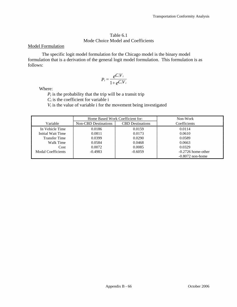
Transportation Conformity Analysis
Appendix B - 66 October 2006
Table 6.1
Mode Choice Model and Coefficients Model Formulation
The specific logit model formulation for the Chicago model is the binary model formulation that is a derivation of the general logit model formulation. This formulation is as follows:
Where: Pt is the probability that the trip will be a transit trip Ci is the coefficient for variable i Vi is the value of variable i for the movement being investigated
Home Based Work Coefficient for: Non-Work Variable Non-CBD Destinations CBD Destinations Coefficients
In Vehicle Time 0.0186 0.0159 0.0114 Initial Wait Time 0.0811 0.0173 0.0610
Transfer Time 0.0399 0.0290 0.0589 Walk Time 0.0584 0.0468 0.0663
Cost 0.0072 0.0085 0.0329 Modal Coefficients -0.4983 -0.6059 -0.2726 home-other
-0.8072 non-home
ee
VCVC
Pii
iit
+=
1

Transportation Conformity Analysis
Appendix B - 67 October 2006
Table 6.2 Example Application of the Home Based Work Trip Model
Example using CBD coefficients
Variable Highway Transit Difference Coefficient diff.*coeff. in-vehicle time 25 45 -20 0.0159 -0.3180 first headway 0 5 -5 0.0173 -0.0865 transfer time 0 10 -10 0.0290 -0.2900 walk time 5 7 -2 0.0468 -0.0936 cost 200 100 100 0.0085 0.8500 Modal Coefficient -0.6059 -0.6059 Sum Difference of values times the coefficients -0.5440 exp(equation) 0.5804 1+ exp(equation) 1.5804 transit probability (exp(equation)/ (1.0+exp(equation) 0.3673
Example using non-CBD coefficients Variable Highway Transit Difference Coefficient diff.*coeff.
in-vehicle time 25 45 -20 0.0186 -0.3720 first headway 0 5 -5 0.0811 -0.4055 transfer time 0 10 -10 0.0399 -0.3990 walk time 5 7 -2 0.0584 -0.1168 cost 200 100 100 0.0072 0.7200 Modal Coefficient -0.4983 -0.4983 Sum Difference of values times the coefficients -1.0716 exp(equation) 0.3425 1+ exp(equation) 1.3425 transit probability (exp(equation)/ (1.0+exp(equation) 0.2551

Transportation Conformity Analysis
Appendix B - 68 October 2006
6.4 MONTE CARLO SIMULATION
A major source of the inaccuracy of mode choice models is the use of average values such as the average cost of parking in a traffic analysis zone or the average income of the traveler. The CATS travel demand analysts recognized this potential source for inaccuracy very early, perhaps before anyone else was aware of the potential problems that could be generated by the use of average values. The solution the CATS analysts derived was to identify the major areas which are affected by average values and to use a method which would "convert" the average values into individual values. This methodology is called a Monte Carlo simulation technique and, after the Chicago application, the technique was also used in the Dallas-Fort Worth region and the Cleveland region.
A Monte Carlo simulation focuses on selecting a representative value for a measure with this value being selected at random from a distribution of values for the measure. For example if there were six parking garages in an area with each lot having the following characteristics:
Parking Lot A: 150 spaces with a cost of $3.50 a day Parking Lot B: 175 spaces with a cost of $3.75 day Parking Lot C: 275 spaces with a cost of $3.25 a day Parking Lot D: 75 spaces with a cost of $1.25 day Parking Lot E: 150 spaces with a cost of $3.50 a day Parking Lot F: 175 spaces with a cost of $3.25 day
In this case the average parking cost, for the 1000 spaces, is $3.26. But a few "lucky" people (seven and one-half percent) could park for $1.25 and some "unfortunate" people (seventeen and a half percent) have to pay $3.75. The difference between the average cost and the low cost is $2.00 while the difference between the average cost and the high cost is 50 cents. These differences are substantial given that a major determinant of mode usage is the cost of using the mode. In a Monte Carlo simulation a specific parking lot would be "picked" at random. The probability of being "picked" would be a function of a relative parameter, in this case the number of spaces. Therefore in approximately seven percent of the "picks" the inexpensive lot would be selected while in eighteen percent of the picks the most expensive lot would be picked.
In the Chicago mode choice model the Monte Carlo simulation technique is used to: (1) estimate the access attributes of the main transit network; (2) estimate the egress attributes from the main transit network; (3) estimate the traveler's annual income; (4) estimate the parking costs and the walk from the parking lot to the person's final destination; and (5) estimate the final selection of the mode used by the traveler. The access and egress attributes are estimated when the trip is made on a subway, elevated or commuter rail mode. These attributes include the mode access used, such as walking, feeder bus, drive or be driven to the station. The attributes also include the time spent walking, driving, riding in the bus and waiting for the bus (if the access/egress mode is feeder bus) and the cost of using the access mode including the cost of parking at the stations. The access/egress attributes are estimated given the number of bus miles in the analysis area (traffic analysis zone), the size of the analysis area, the distance to the rail station, the cost of parking at the rail station, and the type of area.

Transportation Conformity Analysis
Appendix B - 69 October 2006
The income of the traveler is estimated using the average income of the traveler's home area. The parking cost and walk time is estimated given a range of parking costs and spaces for each analysis area in the central business district. This procedure incorporates an estimate of the percent of "free spaces" available by income level. Staff updated the quantity of CBD parking by price in 1999.
Since the Monte Carlo simulation is applied using random probabilities to obtain specific values of time and cost rather than average values, it is fairly obviously that the procedure must be applied several times to obtain stable and accurate results. For the new trip procedures the mode choice procedures were applied for each estimated person trip. For example if the distribution model estimated that 50 trips would be made from zone A to zone B, the mode choice model would be applied 50 times for this interchange, one per trip, and the resulting probabilities would be applied to each of the 50 trips. The Monte Carlo technique was also used to made the final estimate of mode choice. The mode choice model estimates the probability that a trip would be a transit trip. This probability is then used with a Monte Carlo technique to estimate if the trip is a transit trip. For example if the mode choice model estimates that the probability of a trip being a transit trip is 0.25 then when the random number, generated by the Monte Carol technique was less than 0.26 the trip would be considered a transit trip, otherwise the trip would be considered a highway trip. Since there are approximately 17 million person trips in 1990, this results in a very large set of multiple applications.
This use of multiple applications is illustrated below:
Percent
Transit
Iterations of Monte Carlo Applications


Transportation Conformity Analysis
Appendix B - 70 October 2006
7 TIME OF DAY HIGHWAY ASSIGNMENT
The principal objective behind multiple time period highway assignments is to develop more accurate estimates of vehicle-miles by different speed ranges and vehicle classes for air quality conformity analyses. Separate assignments estimate highway vehicle-miles and travel speeds for eight time periods during the day: (1) the ten hour late evening-early morning off-peak period; (2) the shoulder hour preceding the AM peak hour; (3) the AM peak two hours; (4) the shoulder hour following the AM peak hour; (5) a five hour midday period; (6) the two hour shoulder period preceding the PM peak hour; (7) the PM peak two hours, and; (8) the two hour shoulder period following the PM peak hour. Results of the separate period assignments are accumulated into daily volumes, and also tabulated into the vehicle-mile by vehicle type by speed range tables needed for the vehicle emission calculations. The completion and summarizing of the eight time period assignments is highly simplified through the use of EMME/2 macros for repetitive sequences of control statements.
Figure 7.1 is a schematic diagram that shows the sequence of steps in the multiple time period assignment. The nine network scenarios are first assembled. Although there are eight time periods modeled during the day, only three different highway networks are used, an AM peak period, a PM peak period and an off-peak period. The AM peak network is assigned in the pre AM peak, AM peak and post AM peak assignments, and the PM peak network in the three comparable PM periods. The night and midday periods are assigned onto the off-peak network.
The coding of the Kennedy Expressway reversible lanes is one example of how these networks differ. The reversible lanes are inbound in the AM and outbound in the PM network. They are not included in the off-peak network even though the lanes operate part of the night and midday time periods. Including a link that is available only during part of a time period can cause an over assignment of traffic on that link.
The prototype 1990 base year assignment macro includes ten daily ten trip tables, three auto driver/passenger tables by trip purpose, four truck trip tables by vehicle type, two external trip tables for autos and trucks, and a trip table of air passenger trips. The assignment macros can be modified to factor different trip tables, either additional trip purposes after the trip distribution and mode choice models are revised, or special trip tables for major developments.
The main macro (Daily.Period.Asmt) starts the process by calling the macro for the first off-peak time period assignment (Period1.Asmt). The appropriate network scenario is selected and the matrices used to store the off-peak period trip tables are initialized. The matrices are then filled with the off-peak trip tables factored from the daily trip tables. Network link and node user variables are next initialized. Two macros to preprocess the network are then called by the assignment macro. The first one calculates uncongested link times and link capacities, the

Transportation Conformity Analysis
Appendix B - 71 October 2006
Figure 7.1 Multiple Time Period
Highway Assignment
Total Link Volumes(Macro: Daily.Total.Asmt)
Emission Calculations
Mode Choice Model
Create ScenariosEight Time PeriodsDaily (Accumulated)
Daily Trip TablesPurposeVehicle Class
Multiple Period Assignment(Macro: Daily.Period.Asmt)
Select Scenario(Macro: Periodn.Asmt)
InitializeLink and NodeMatrices
EstimateUncongested Timesand Lane Capacities
(Macro Ftime.Capacity)
Estimate SignalCycle Lengths and
Green/Cycle Ratios(Macro: Arterial.Delay)
Factor Trip Tablesto Time Period n
AssignmentVolume-Delay
Functions
AssignmentInitial Solution
AssignmentRemaining Iterations
Volume-DelayFunctions
PreviousLink Times
Period 1 Periods 2-8
Periods 2-8
second estimates signal cycle lengths and green time to cycle length ratios for the j-node of arterial street and freeway to arterial ramp links.
For the first off-peak time period, the standard set of volume-delay functions are loaded
and the scenario is prepared for assignment. A full equilibrium assignment is the final step to complete the off-peak time period assignment. The logic of the process is slightly altered in subsequent periods. An initial set of volume-delay functions is loaded for the first all-or-nothing assignment. These volume-delay functions set link times to the final travel times of the previous time period. The scenario is then readied for the initial assignment. After the initial all-or-nothing assignment is completed, the standard set of volume-delay functions is reloaded. The assignment is then readied for additional iterations and the remaining equilibrium assignment iterations completed.
The procedure repeats through the remaining seven time periods. When the eight time periods are completed, control is passed to the macro that totals the period link volumes into daily volumes by vehicle and cold starts. These summary tabulations are performed in the ninth

Transportation Conformity Analysis
Appendix B - 72 October 2006
scenario. Two other macros also create the tables needed for emission calculations: vehicle-miles are tabulated into one mile per hour speed ranges for six vehicle types.
7.1 ASSIGNMENT TIME PERIODS
The travel data that led to selecting the eight time periods is illustrated in Figure 7.2. This is a plot of the auto driver and auto passenger trips in motion reported in CATS' 1990 household travel survey. Trips were accumulated at the end of ninety-six fifteen minute periods through the day. The plot shows a moving average of these accumulated trips calculated over four consecutive fifteen minute periods. The moving average smoothes out the irregularities in the plot caused by the tendency of surveyed travelers to report trip start and completion times to the nearest quarter-hour or half-hour.
The plot shows the distinct peaking of auto travel during the morning and evening peak periods. The large number of trips in motion during peak travel periods is due not only to increased trip making during these time periods. Peak period auto trips also stay in motion longer because they are more likely to be lengthy work trips subjected to slower congested peak period travel speeds.
The Figure 7.2 plot is not symmetric because the evening peak period is longer and slightly worse than the morning peak. The two peak periods are separated by a midday period that has a fairly uniform number of trips in motion, except for a bulge in trip making around the noon lunch period. Trips in motion plateau between 8:00 PM and 9:00 PM after the evening peak period, and then quickly decline during the off-peak period.
The two assignment peak periods are defined differently because of these auto travel
Figure 7.2 Time Distribution of Auto Driver and Passenger Trips
0 4 8 12 16 20 24 28 32 36 40 44 48 52 56 60 64 68 72 76 80 84 88 920
100,000
200,000
300,000
400,000
500,000
600,000
p
15 Minute Period
Peak
Shoulder

Transportation Conformity Analysis
Appendix B - 73 October 2006
characteristics. The shading under the Figure 7.2 curve shows the peak and shoulder periods used in the multiple time period assignments. A two hour AM peak (7:00 AM to 9:00 AM) and two one hour AM peak shoulder periods (6:00 AM to 7:00 AM and 9:00 AM to 10:00 AM) effectively cover the morning peak period. Six hours are needed to capture the evening peak period, a two hour PM peak (4:00 PM to 6:00 PM) plus two hour PM peak shoulder periods on either side of the PM peak (2:00 PM to 4:00 PM and 6:00 PM to 8:00 PM). This leaves a nearly uniform four hour midday period between the two peaks (10:00 AM to 2:00 PM), and an off-peak period (8:00 PM to 6:00 AM) covering the late evening and early morning hours.
7.2 TRIP TABLE FACTORS
Factors to allocate daily auto person trip tables into the eight time period trip tables were derived from the CATS' 1990 household travel survey. Expanded survey auto driver and auto passenger trips are allocated to time periods by their start and completion times. Trips spanning two or more periods are apportioned to the separate periods according to time spent traveling in each period. For example, a survey trip with an expansion factor of 100 that spends thirty percent of its time in one time period and seventy percent of its time in a second period would have thirty trips allocated to the first period and seventy to the second period.
Table 7.1 lists the factors to create the eight time period trip tables from daily auto driver and auto passenger trip tables. Separate factors apply to central area work trips, destinations within the area bordered by Lake Michigan, Chicago Avenue, Halsted Avenue and Roosevelt Road (zones 54 through 100 in the zone 95 system). Adding together the home-work and home-other fractions does not total one because the trip tables are in home production and non-home attraction format. The factors sum to the proportion of trips from home and to home. Fractions for non-home/work trips do sum to one, since this trip table is by trip direction.
Daily auto driver and auto passenger trip tables (that include auto access to transit trips) from full model iteration are multiplied by the Table 7.1 factors to obtain auto driver and auto passenger trip tables for the eight time periods. They are then divided by the auto occupancies in Table 7.2 to produce the auto vehicle trip tables that are assigned.
Table 7.1. Time Period Trip Table Factors for Auto Driver/Passenger Trips Auto Person Trip Table
Off Peak (8:00 PM to 6:00 AM)
Pre AM Peak(6:00 AM to
7:00 AM)
AM Peak (7:00 AM to
9:00 AM)
Post AM Peak(9:00 AM to 10:00 AM)
Midday (10:00 AM to 2:00 PM)
Pre PM Peak (2:00 PM to
4:00 PM)
PM Peak (4:00 PM to
6:00 PM)
Post PM Peak(6:00 PM to
8:00 PM)
Home to Work To CBD Work 0.064 0.088 0.287 0.034 0.036 0.017 0.003 0.008 To Non-CBD Work 0.050 0.098 0.261 0.028 0.044 0.026 0.018 0.009 From CBD Work 0.085 0.000 0.003 0.003 0.017 0.056 0.195 0.104 From Non-CBD Work 0.070 0.000 0.003 0.002 0.034 0.083 0.208 0.064 To Airport Work 0.131 0.072 0.138 0.040 0.077 0.074 0.012 0.009 From Airport Work 0.147 0.025 0.019 0.001 0.042 0.103 0.091 0.042
Home to Non-Work From Home 0.024 0.009 0.071 0.044 0.114 0.042 0.060 0.107 To Home 0.147 0.001 0.010 0.012 0.111 0.080 0.077 0.090
Non-Home/Work All Trips 0.057 0.004 0.041 0.055 0.436 0.163 0.147 0.097

Transportation Conformity Analysis
Appendix B - 74 October 2006
Table 7.2 Time Period Auto Occupancies
Auto Person Trip Table
Off Peak (8:00 PM to 6:00 AM)
Pre AM Peak(6:00 AM to
7:00 AM)
AM Peak (7:00 AM to
9:00 AM)
Post AM Peak(9:00 AM to 10:00 AM)
Midday (10:00 AM to 2:00 PM)
Pre PM Peak (2:00 PM to
4:00 PM)
PM Peak (4:00 PM to
6:00 PM)
Post PM Peak(6:00 PM to
8:00 PM)
Home to Work To CBD Work 1.09 1.21 1.24 1.27 1.35 1.10 1.23 1.06 To Non-CBD Work 1.11 1.10 1.07 1.07 1.07 1.10 1.14 1.14 From CBD Work 1.13 1.14 1.14 1.00 1.04 1.07 1.21 1.09 From Non-CBD Work 1.15 1.32 1.21 1.04 1.07 1.09 1.09 1.08
Home to Non-Work From Home 1.24 1.39 1.77 1.28 1.24 1.20 1.30 1.33 To Home 1.32 1.10 1.09 1.13 1.22 1.34 1.26 1.27
Non-Home/Work All Trips 1.34 1.16 1.17 1.10 1.17 1.15 1.15 1.28
Factors for external auto trips and auto air passenger trips are listed in Table 7.3.
External auto trip factors are based upon the distribution of auto driver trips for all purposes in the survey, since there is no other suitable data on the time distribution of external travel.
Table 7.3 Time Period Trip Table Factors for Miscellaneous Auto Trips
Vehicle Trip Table
Off Peak (8:00 PM to 6:00 AM)
Pre AM Peak(6:00 AM to
7:00 AM)
AM Peak (7:00 AM to
9:00 AM)
Post AM Peak(9:00 AM to 10:00 AM)
Midday (10:00 AM to 2:00 PM)
Pre PM Peak (2:00 PM to
4:00 PM)
PM Peak (4:00 PM to
6:00 PM)
Post PM Peak(6:00 PM to
8:00 PM)
External To and From Region 0.121 0.040 0.140 0.049 0.224 0.129 0.172 0.126
Airports To Terminal 0.163 0.069 0.130 0.050 0.227 0.137 0.114 0.111 To Non Terminal 0.245 0.134 0.258 0.043 0.144 0.139 0.023 0.016 From Terminal 0.157 0.073 0.136 0.051 0.216 0.135 0.134 0.096 From Non Terminal 0.302 0.054 0.040 0.003 0.091 0.222 0.196 0.090
The last set of trip table factors for trucks is listed in Table 7.4. These were determined
from the 1986 CATS' commercial vehicle survey. Factors for external truck trips are regional factors based upon the vehicle equivalent weighted total truck trip table.
Table 7.4 Time Period Trip Table Factors for Truck Trips in Vehicle Equivalents
Truck Trip Table Off Peak
(8:00 PM to 6:00 AM)
Pre AM Peak(6:00 AM to
7:00 AM)
AM Peak (7:00 AM to
9:00 AM)
Post AM Peak(9:00 AM to 10:00 AM)
Midday (10:00 AM to 2:00 PM)
Pre PM Peak (2:00 PM to
4:00 PM)
PM Peak (4:00 PM to
6:00 PM)
Post PM Peak(6:00 PM to
8:00 PM)
Truck Classes B Plate 0.022 0.026 0.144 0.115 0.358 0.229 0.094 0.012 Light 0.024 0.057 0.422 0.089 0.214 0.141 0.040 0.013 Medium 0.069 0.036 0.166 0.140 0.421 0.108 0.038 0.022 Heavy 0.210 0.039 0.135 0.082 0.315 0.104 0.071 0.043
External To and From Region 0.057 0.034 0.187 0.110 0.340 0.180 0.074 0.018
Table 7.5 lists the truck and auto trips in each period's trip table. Trucks are tabulated in
vehicle equivalents. As previously noted, auto and truck trip tables are assigned separately in a multiple vehicle class EMME/2 assignment, although both trip tables have to be in vehicle

Transportation Conformity Analysis
Appendix B - 75 October 2006
equivalents, and there is no single combined vehicle equivalent trip table. The relative importance of trips in the period trip tables is difficult to compare in Table 7.5 because the time periods cover different lengths of time.
Table 7.5 Auto and Truck (Vehicle Equivalents) by Time Period
Trip Table
Off Peak (8:00 PM to 6:00 AM)
Pre AM Peak (6:00 AM to
7:00 AM)
AM Peak (7:00 AM to
9:00 AM)
Post AM Peak (9:00 AM to 10:00 AM)
Midday (10:00 AM to
2:00 PM)
Pre PM Peak (2:00 PM to
4:00 PM)
PM Peak (4:00 PM to
6:00 PM)
Post PM Peak (6:00 PM to
8:00 PM)
Truck 126,574 73,290 404,937 229,775 709,353 372,159 154,243 39,452
Auto 1,595,114 486,823 1,704,014 653,981 3,070,325 1,683,091 2,208,415 1,675,629
Total 1,721,688 560,113 2,108,951 883,756 3,779,678 2,055,250 2,362,758 1,715,081
To make it easier to compare these time period trip tables, the Table 7.5 figures have
been converted into trips per hour and plotted in Figure 7.3. This figure shows the trips in the truck and auto trip tables per hour and the total trips in the two trip tables per hour.
Perhaps the most striking feature of this graph is the different peaking characteristics of
truck and auto trips. Truck travel does not exhibit the twice a day peaking associated with person travel. Truck trips build up in the morning peak and then continue throughout the day until declining before the evening peak. This daily truck trip pattern is caused by the more uniform schedule of goods pickups and deliveries during a typical work day. One effect of the different auto and truck peaking characteristics is to lengthen the AM peak period. The AM peak and post AM peak shoulder hours have nearly the same number of vehicle trips, although trucks account for a larger portion of the post AM peak shoulder traffic. The peaking characteristics of truck trips increase midday traffic between the morning and evening peak periods, which reduces the prominence of the two peak periods for total vehicle trips.
Figure 7.3 Relative Sizes of Time Period Trip Tables
Off-Peak Pre AM AM Peak Post AM Midday Pre PM PM Peak Post PM0
200,000
400,000
600,000
800,000
1,000,000
1,200,000
1,400,000
Period
Vehicles/Hour
Trucks Autos Total

Transportation Conformity Analysis
Appendix B - 76 October 2006
7.3 VOLUME-DELAY FUNCTIONS
The volume-delay functions have been revised for several reasons. Signal characteristics are introduced into the volume-delay functions for links that end at signalized intersections. This means that assignments are now sensitive to signal characteristics and can reflect major signal modernization programs. In addition to more accurately representing the characteristics of the network, these signal sensitive volume-delay functions allow the emission reductions from signal improvements to be evaluated.
The second reason for changing the volume-delay functions is because of the previous functions’ limitations when they are used for time period assignments. Their most severe limitation is that freeways and expressways tend to be over assigned in the congested peak time periods. Several factors contribute to this peak period over assignment of freeways including: (1) an extremely unrealistic initial peak period assignment since paths are built using uncongested travel times; (2) the inability to model bottlenecks in the freeway network that occur during peak periods, and; (3) not restricting freeway on-ramps whose peak period capacities are controlled by metering. The approach taken is to alter the volume-delay functions for freeways, expressway and metered freeway entrance ramps so that travel times increase far more quickly after capacity is reached. The capacities of metered on-ramps are also set to maximum metered flow rates.
A second limitation addressed in the revision of volume-delay functions is the under assignment of Illinois Tollway links. Tollway links were greatly under assigned in off-peak period assignments because the average value of time used to convert tolls into toll link time penalties generally put tollways at too great a disadvantage compared to untolled routes. In reality, the value of time for auto drivers and passengers has a range of values and many persons have a high enough value of time to justify using tollways even given the modest off-peak time savings of toll routes This problem was solved by introducing a toll link volume-delay function that reflects a range of user time values derived from income levels.
Volume-Delay Functions for Links Ending at Signalized Intersections (vdf1 and vdf3)
Intersection delays in the volume-delay functions are based upon the Webster equation.7 In this equation, intersection delay has uniform and incremental components, and both are fairly complicated to calculate. For the volume-delay functions, simpler regression equations were fit to calculated uniform and incremental delays for a range of signal cycle lengths and green time to cycle length ratios.
The regression equations for uniform and incremental signal delays are combined with link travel time estimates in the first (arterial) and third (freeway exit ramp to arterial) volume-delay functions as follows:
1. Link travel time between intersections is: 7 F. V. Webster and B. M. Cobbe. Traffic Signals. Road Research Laboratory, Ministry of Transport Road
Research, Technical Paper No. 56, 1966.

Transportation Conformity Analysis
Appendix B - 77 October 2006
Tlink = T0*⎝⎛
⎠⎞1 + 0.15*⎝
⎛⎠⎞volau
capacity4
.
This is the widely used BPR function where Tlink equals the link’s travel time without any intersection delay and T0 is the uncongested link travel time without intersection delay. The uncongested link travel time is computed using the maximum speed permitted on the link. Quantity volau is the link’s traffic volume for the time period in auto equivalents. Capacity in the link travel time function is approximately the service volume at level of service C. It is calculated as 75 percent of the level of service E time period capacity, which is the hourly lane capacity multiplied by the number of lanes multiplied by the hours in the time period.
2. Uniform intersection delay equals:
Du = 6.0*⎝⎛
⎠⎞volau
capacity - 0.39*green + 0.35*cycle - 4.5.
Where Du is the average uniform intersection delay at the link’s j-node in seconds. Green is the green time allowed the link at the j-node intersection and cycle is the cycle length at the intersection. Both quantities are in seconds. The uniform delay is restricted to positive values in the volume-delay functions.
3. Incremental delay at intersections equals:
Di = 2.7*⎝⎛
⎠⎞volau
capacity 8 - 7.3*⎝
⎛⎠⎞green
cycle + 3.4.
Where Di is the average incremental intersection delay at the link’s j-node in seconds. Incremental delay is also restricted to positive values in the volume-delay functions.
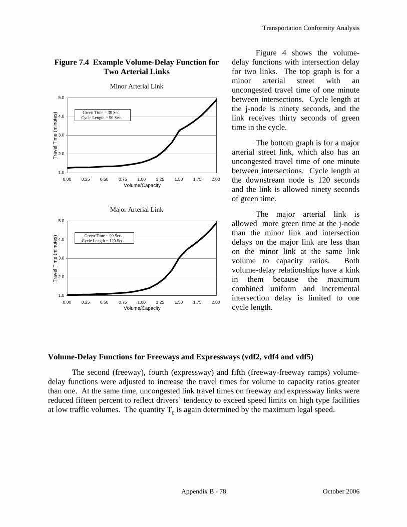
Transportation Conformity Analysis
Appendix B - 78 October 2006
Figure 4 shows the volume-delay functions with intersection delay for two links. The top graph is for a minor arterial street with an uncongested travel time of one minute between intersections. Cycle length at the j-node is ninety seconds, and the link receives thirty seconds of green time in the cycle.
The bottom graph is for a major arterial street link, which also has an uncongested travel time of one minute between intersections. Cycle length at the downstream node is 120 seconds and the link is allowed ninety seconds of green time.
The major arterial link is allowed more green time at the j-node than the minor link and intersection delays on the major link are less than on the minor link at the same link volume to capacity ratios. Both volume-delay relationships have a kink in them because the maximum combined uniform and incremental intersection delay is limited to one cycle length.
Volume-Delay Functions for Freeways and Expressways (vdf2, vdf4 and vdf5)
The second (freeway), fourth (expressway) and fifth (freeway-freeway ramps) volume-delay functions were adjusted to increase the travel times for volume to capacity ratios greater than one. At the same time, uncongested link travel times on freeway and expressway links were reduced fifteen percent to reflect drivers’ tendency to exceed speed limits on high type facilities at low traffic volumes. The quantity T0 is again determined by the maximum legal speed.
Figure 7.4 Example Volume-Delay Function for
Two Arterial Links
Minor Arterial Link
1.0
2.0
3.0
4.0
5.0
Trav
el T
ime
(min
utes
)
0.00 0.25 0.50 0.75 1.00 1.25 1.50 1.75 2.00 Volume/Capacity
Green Time = 30 Sec.Cycle Length = 90 Sec.
Major Arterial Link
1.0
2.0
3.0
4.0
5.0
Trav
el T
ime
(min
utes
)
0.00 0.25 0.50 0.75 1.00 1.25 1.50 1.75 2.00 Volume/Capacity
Green Time = 90 Sec.Cycle Length = 120 Sec.

Transportation Conformity Analysis
Appendix B - 79 October 2006
These adjustments were made to the basic BPR volume-delay relationship, as follows:
Tlink = T0
1.15 *⎝⎛
⎠⎞1 + 0.15*⎝
⎛⎠⎞volau
capacity * 1 + 0.15*8
volaucapacity
⎛⎝⎜
⎞⎠⎟
⎛
⎝⎜⎜
⎞
⎠⎟⎟ , for ⎝
⎛⎠⎞volau
capacity ≤ 1.
Tlink = T0* 1 + 0.15*8
volaucapacity
⎛⎝⎜
⎞⎠⎟
⎛
⎝⎜⎜
⎞
⎠⎟⎟ , for ⎝
⎛⎠⎞volau
capacity > 1.
Figure 7.5 compares the revised BPR volume-delay function with the original BPR function for a one mile link with a maximum speed of 60 miles per hour. At a volume to capacity ratio of one, both functions predict the same link travel times. At lower volume to capacity ratios, the revised function’s travel time is slightly less than the original function due to the lower initial uncongested travel time. For volume to capacity ratios greater than one, the travel time predicted by the revised function is higher and rapidly increases because the volume to capacity ratio is exponentiated to a much higher power.
Volume-Delay Function for Metered Freeway Entrance Ramps (vdf8)
For metered freeway entrance ramps, the original BPR function is revised so that travel times greatly increase when the link volume exceeds the maximum metered flow rate. This effectively restricts the ramp’s volume to the metered flow rate. The adjusted BPR function is:
Tlink = T0*⎝⎛
⎠⎞1 + 0.15*⎝
⎛⎠⎞volau
metered flow10
.
The maximum metered flow rate is taken as 720 vehicles per hour per lane, or an average vehicle delay at the ramp metering signal of five seconds. Volume-Delay Function for Links With Tolls (vdf7)
The volume-delay function for links where tolls are collected was changed more than any other link type volume-delay functions. Early off-peak time period assignments under assigned tollway links to the point where some tollway links did not have any traffic assigned on them. It was obvious that the average value of time used to convert tolls into equivalent minutes of delay was not appropriate for the off-peak period.
Figure 7.5 Revised BPR Volume-Delay Function
for Freeway/Expressway Links
0.0
2.0
4.0
6.0
8.0
10.0
12.0
14.0
Trav
el T
ime
(min
utes
)
0.00 0.25 0.50 0.75 1.00 1.25 1.50 1.75 2.00 Volume/Capacity
Original BPR
Revised BPR

Transportation Conformity Analysis
Appendix B - 80 October 2006
A volume-delay function that adjusts the implied value of time with increasing link volume was developed for toll links. To apply this toll link volume-delay function, the maximum volume that would pass through the toll link if no toll is charged is first estimated. Final link volumes from an equilibrium assignment were used. Adding toll penalties reduces the volumes through toll links from these upper bound volumes.
Once the upper bound volumes through the toll links are known, the applicable value of time for converting tolls to delay can be stated as a function of link volume if the distribution of time values is known. Figure 7.6 shows the basis for the distribution of time values used in the volume-delay function.
Figure 7.6 Value of Time Distribution in Toll Link VDF
(Percent of Workers or Households with Income Based Value of Time Greater Than Shown)
0
10
20
30
40
50
Min
utes
/Dol
lar
0% 20% 40% 60% 80% 100%Percent of Workers or HHs
HHs
Worker
VDF
This figure is interpreted in the following manner. The Y-axis is the value of time based upon income expressed in minutes per dollar. The X-axis is the cumulative percent of workers or households with a value of time greater than the value shown on the Y-axis. For example, ninety percent of all households in the region have an income based value of time greater than twelve to thirteen minutes per dollar, roughly equivalent to an annual income of $9000 to $10,000. The original worker and household income data are 1990 census annual figures factored to hourly levels.
The darker line in the figure shows the relationship in the toll link volume-delay function. It was developed by fitting a function to 150 percent (two-thirds the income based time value) of the household minutes per dollar figures. There is no justification for basing the value of time on household income instead of worker income or some other income data. The distribution of time values is the important factor, however, and the Figure 7.6 relationship can be shifted somewhat without greatly affecting the assignment results. Note, that the one dollar of toll translates into less than five minutes of travel time for more than half the volume-delay function.

Transportation Conformity Analysis
Appendix B - 81 October 2006
The resulting volume-delay function for toll links is the following:
Tlink = toll * 2 + 40*6volau
imumvolumemax⎛⎝⎜
⎞⎠⎟
⎛
⎝⎜⎜
⎞
⎠⎟⎟ .
The toll paid in the equation is in dollars, and the equivalent link travel time, Tlink, is in minutes. The quantity maximum volume is the traffic flow measured through the link without tolls.
Values of time implied by the toll volume-delay function range between thirty dollars per hour (two minutes per dollar) and $1.40 (forty-two minutes per dollar) when the assigned volume equals the maximum untolled volume. This volume-delay function also assumes that the same distribution of time values exists for traffic through all toll links. Toll plazas at interchanges serving wealthy areas are not distinguished from toll facilities used by less well to do travelers.
7.4 ASSIGNMENT ITERATIONS
Table 7.6 shows the number of equilibrium assignment iterations by time period for the base 1990 and 2020 assignments. The congested peak periods require more equilibrium assignment iterations than the lesser congested time periods to reach the same level of closure. For the highway assignment runs discussed in this section, average zone to zone path times and average link travel times are within at least one half minute of one another, except for the AM peak period assignment, which terminates at twenty-five iterations with the two times less than a minute apart. Average path and link times are equal when network equilibrium is achieved.
Table 7.6 Assignment Iterations
Time Period Base 1990 Iterations 2020 Iterations Off-Peak 3 3 Pre AM Peak 8 17 AM Peak 25 25 Post AM Peak 7 13 Midday 5 9 Pre PM Peak 7 14 PM Peak 15 24 Post PM Peak 6 6 Total 76 111

Transportation Conformity Analysis
Appendix B - 82 October 2006
The time period assignments provide a more detailed and accurate picture of congestion effects in the highway network, which is advantageous for several reasons. While daily estimated traffic volumes may just be marginally improved compared to volumes produced by average daily assignments, estimates of network speeds are substantially improved and regional vehicle-miles of travel agree more closely with state estimates of daily vehicle-miles. Since congestion is more correctly modeled, impacts from proposed highway improvements that reduce congestion are also more accurately reproduced by the time period assignments.
7.5 LINK SPEEDS
A product of the time of day assignment is a traffic volume for each link by each time period of the day. The speed of travel for each link is calculated by an equation that uses the volume-capacity ratio for the link as the independent variable. The following equations are used to produce the final link speed: For freeways:
S=S0 _____1______ x _____1______ for V/C ≤ 1 1+.15 (V/C) 1+.15 (V/C)8
S=S0 _____1_______ for V/C > 1 1+.15 (V/C)8
For arterials:
S=S0 _________________1___________________ (1n(S0) * .249) + .153 ( V/(C * .75)) 3.98
Where S = Speed on link used for emission calculation S0 = Initial Speed on link V/C = Volume-Capacity ratio for the link
These curves represent modifications to the Bureau of Public Roads (BPR) curves that have been used at CATS and other agencies for many years. Consistent with a national trend for agencies to use modified curves based on local data, these curves are based on the information gathered from local empirical data. The freeway curve is the same as used in the volume delay functions in the time of day assignment iterations. The arterial curve is slightly modified to better correlate with the empirical data. The data is from IDOT’s traffic sensor system for the expressway system and CATS conducted speed runs for the arterial system. This data base is documented in CATS Working Paper 95-09, Travel Time Database and Structure Chicago Area

Transportation Conformity Analysis
Appendix B - 83 October 2006
Expressway System, September 1995, and CATS Working Paper 97-09, 1994, 1995 and 1996 Combined Travel Time Database Documentation: Arterial Highway System, July 1997. The methodology for the curve development is presented in CATS Working Paper 97-12, Method for Adjusting Modeled Speeds Based on Empirical Speed Data, August 1997. Figure 7.7 presents a comparison of the CATS arterial V/C versus speed curve and the BPR curve for two initial speeds. As can be seen, the curves are similar for an initial speed of 55 mph. For the initial speed of 30 mph., the curves are similar for V/C ratios above one. For lower V/C ratios, the CATS curve has higher speeds than the BPR curve consistent with observed data. FIGURE 7.7 CATS TO BPR CURVE COMPARISON
0 1 2 3 4 50
2 0
4 0
6 0
v o lu m e /c a p a c ity
mile
s pe
r hou
r
B PR C A T S
initial speed=55 mph
0 1 2 3 4 50
1 0
2 0
3 0
4 0
v o lu m e /c a p a c ity
mile
s pe
r hou
r
B PR C A T S
initial speed=30 mph
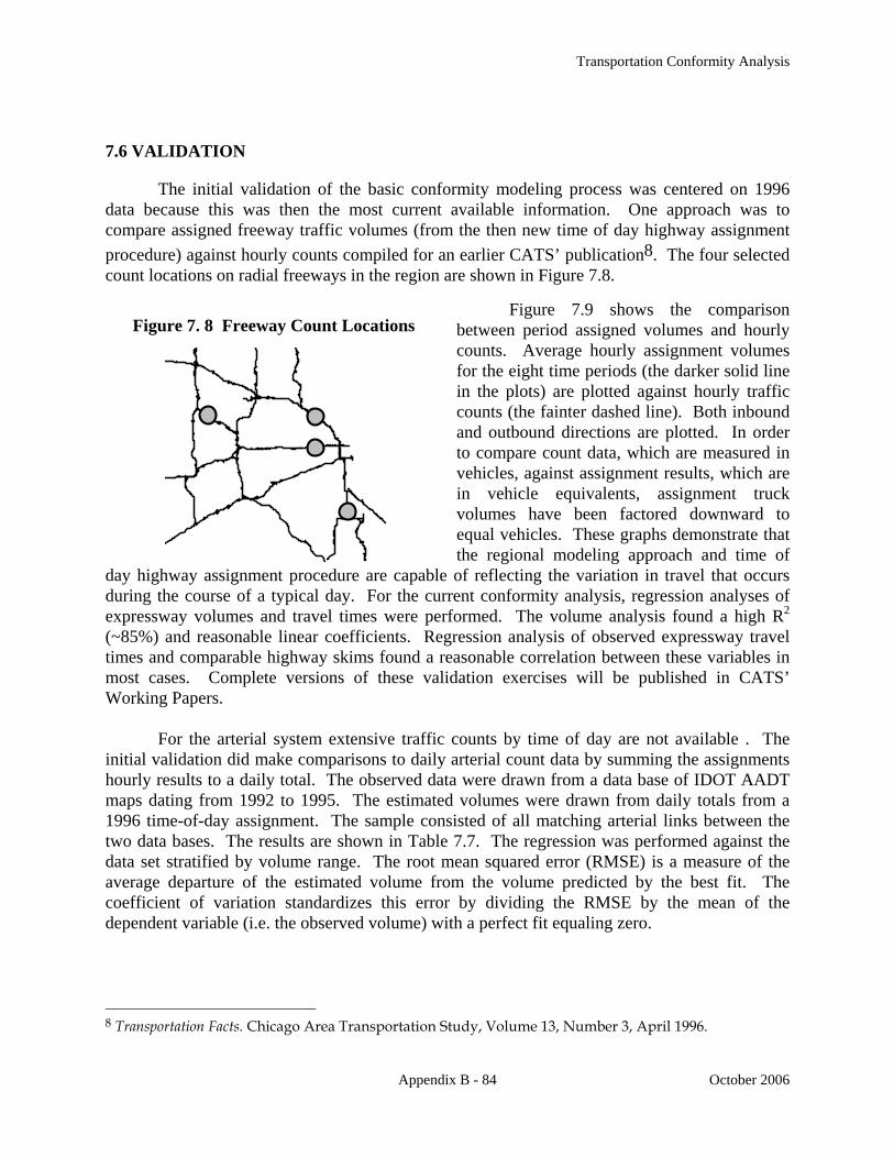
Transportation Conformity Analysis
Appendix B - 84 October 2006
7.6 VALIDATION
The initial validation of the basic conformity modeling process was centered on 1996 data because this was then the most current available information. One approach was to compare assigned freeway traffic volumes (from the then new time of day highway assignment procedure) against hourly counts compiled for an earlier CATS’ publication8. The four selected count locations on radial freeways in the region are shown in Figure 7.8.
Figure 7.9 shows the comparison between period assigned volumes and hourly counts. Average hourly assignment volumes for the eight time periods (the darker solid line in the plots) are plotted against hourly traffic counts (the fainter dashed line). Both inbound and outbound directions are plotted. In order to compare count data, which are measured in vehicles, against assignment results, which are in vehicle equivalents, assignment truck volumes have been factored downward to equal vehicles. These graphs demonstrate that the regional modeling approach and time of
day highway assignment procedure are capable of reflecting the variation in travel that occurs during the course of a typical day. For the current conformity analysis, regression analyses of expressway volumes and travel times were performed. The volume analysis found a high R2 (~85%) and reasonable linear coefficients. Regression analysis of observed expressway travel times and comparable highway skims found a reasonable correlation between these variables in most cases. Complete versions of these validation exercises will be published in CATS’ Working Papers.
For the arterial system extensive traffic counts by time of day are not available . The initial validation did make comparisons to daily arterial count data by summing the assignments hourly results to a daily total. The observed data were drawn from a data base of IDOT AADT maps dating from 1992 to 1995. The estimated volumes were drawn from daily totals from a 1996 time-of-day assignment. The sample consisted of all matching arterial links between the two data bases. The results are shown in Table 7.7. The regression was performed against the data set stratified by volume range. The root mean squared error (RMSE) is a measure of the average departure of the estimated volume from the volume predicted by the best fit. The coefficient of variation standardizes this error by dividing the RMSE by the mean of the dependent variable (i.e. the observed volume) with a perfect fit equaling zero. 8 Transportation Facts. Chicago Area Transportation Study, Volume 13, Number 3, April 1996.
Figure 7. 8 Freeway Count Locations

Transportation Conformity Analysis
Appendix B - 85 October 2006
Table 7.7 Arterial Volume Comparison Rounded
directional volume
Number of observations
Observed directional
volume
Modeled directional
volume
Root mean square error
% Root mean square
error 5000 3236 4877.77 5668.67 1338.12 27.4%
10000 2422 9778.95 10589.53 1399.70 14.3%15000 1366 14611.23 14989.78 1320.40 9.0%20000 363 19611.29 19258.32 1333.07 6.8%25000 122 24467.21 23105.19 1230.15 5.0%
Further regression analysis of daily arterial volumes and travel times was done with more
recent data for the current conformity analysis. This included adding geographic stratification to the arterial volume stratification previously used. Additionally, a case study of the relationship between observed travel times and model results for the suburban portion of US12 was done. The specific objective was to examine the three components of arterial delay employed in CATS’ volume delay functions. Full presentation of this work and results obtained will be included in CATS’ Working Papers.

Transportation Conformity Analysis
Appendix B - 86 October 2006
Figure 7.9 Assigned and Counted Hourly Volumes on Major Freeways
Kennedy Expressway at Sacramento Inbound Outbound
0
2,000
4,000
6,000
8,000
10,000
12,000
14,000
16,000
Hou
rly V
olum
e
1 2 3 4 5 6 7 8 9 10 11 12 13 14 15 16 17 18 19 20 21 22 23 24 Hour Ending At
Counted
Assigned
0
2,000
4,000
6,000
8,000
10,000
12,000
14,000
16,000
Hou
rly V
olum
e
1 2 3 4 5 6 7 8 9 10 11 12 13 14 15 16 17 18 19 20 21 22 23 24 Hour Ending At
Counted
Assigned
Eisenhower Expressway at Sacramento Inbound Outbound
0
2,000
4,000
6,000
8,000
10,000
Hou
rly V
olum
e
1 2 3 4 5 6 7 8 9 10 11 12 13 14 15 16 17 18 19 20 21 22 23 24 Hour Ending At
Counted
Assigned
0
2,000
4,000
6,000
8,000
10,000
Hou
rly V
olum
e
1 2 3 4 5 6 7 8 9 10 11 12 13 14 15 16 17 18 19 20 21 22 23 24 Hour Ending At
Counted
Assigned
I-290 at Church Road Inbound Outbound
0
1,000
2,000
3,000
4,000
5,000
6,000
7,000
Hou
rly V
olum
e
1 2 3 4 5 6 7 8 9 10 11 12 13 14 15 16 17 18 19 20 21 22 23 24 Hour Ending At
Counted
Assigned
0
1,000
2,000
3,000
4,000
5,000
6,000
7,000
Hou
rly V
olum
e
1 2 3 4 5 6 7 8 9 10 11 12 13 14 15 16 17 18 19 20 21 22 23 24 Hour Ending At
Counted
Assigned
Dan Ryan Expressway North of I-57, I-94 Interchange Inbound Outbound
0
2,000
4,000
6,000
8,000
10,000
Hou
rly V
olum
e
1 2 3 4 5 6 7 8 9 10 11 12 13 14 15 16 17 18 19 20 21 22 23 24 Hour Ending At
Counted
Assigned
0
2,000
4,000
6,000
8,000
10,000
Hou
rly V
olum
e
1 2 3 4 5 6 7 8 9 10 11 12 13 14 15 16 17 18 19 20 21 22 23 24 Hour Ending At
Counted
Assigned


Transportation Conformity Analysis
Appendix B - 87 October 2006
8 EMISSIONS CALCULATION
8.1 OVERVIEW
The conformity test requires a calculation of total regulated emissions for each scenario
alternative tested. These total emissions must be lower than the corresponding approved emission budgets for ozone precursors or the corresponding baseline value for fine particulate matter (PM2.5) and its precursor, nitrogen oxides (NOx). The geographic distribution of the emissions is not considered in conformity calculations.
The MOBILE model developed by the U.S. Environmental Protection Agency produces emission rates in grams per mile for various vehicle types, facility types and speeds. The time of day assignment from emme/2® is used to produce a table of vehicle miles traveled (VMT) broken down by speed, facility type and vehicle type. Multiplying each VMT value by the corresponding emission rate and summing yields the amounts of the various emissions emitted. Emission reduction credits may be calculated for strategies not accounted for in the model. This chapter explains how the mobile source emission rates are developed and how the total emissions are calculated from the assignment results.
8.2 METHOD
Highway networks were built with zone connectors given distances proportional to zone
size as an analogy that the amount of “local” travel needed to reach the regional highway system is related to zone size. Thus, this conformity analysis does not have a separate off-network mobile emission component. Mobile source emission estimates based upon the network traffic assignment reflect both specifically coded non-local roadways and local non-coded roadways.
Highway assignment produces two basic pieces of information essential to calculating emissions: link loads and link speeds. While essential, the information on link loading is not a perfect match for use with the MOBILE emission rates. The assignment model step defines vehicles in terms of how much of a roadway’s available capacity to carry traffic is used for a given loading. The MOBILE model defines vehicles in terms of engine type and size. For assignment, it makes no difference if a vehicle is diesel or gasoline powered, but this is a highly significant difference for the MOBILE model’s calculation of emission rates. Highway assignment accounts for the different operating characteristics of various vehicle types using the concept of vehicle equivalents9 (VEQ). In the simplest case a standard passenger auto is one VEQ, while a semi-trailer truck is multiple VEQs. The truck occupies approximately the same physical space on the roadway as several standard passenger cars and interacts with other traffic in ways akin to multiple standard vehicles. For example, the truck takes more time to reach
9 Comparable terms also used are passenger car equivalents (pce) and passenger car units (pcu).

Transportation Conformity Analysis
Appendix B - 88 October 2006
cruising speed from a stop than an individual standard passenger auto; the amount of time is similar to that needed by several standard passenger cars to reach cruising speed when driver reaction delay and vehicle spacing are considered. It should be obvious, however, that the emissions from large a truck and several standard autos are not the same (especially if the truck is diesel powered). The time-of-day (TOD) highway assignment process makes use of the additional options assignment procedure in emme/2® to keep track of four truck classes: b-plate, light, medium and heavy, and urban buses. These truck classes are subsequently converted into the MOBILE truck classes before emissions are computed.
When the travel simulation process is complete, several additional steps need to be taken to calculate scenario emissions. The model results must be transformed to be compatible with the MOBILE model’s emission rate structure. The MOBILE model must be run to produce emission rates that match the transportation data available and reflect the region’s environmental and vehicular conditions. The steps that were followed to compute the scenario network-based mobile source emissions are given below.
8.3 PROCEDURE
8.3.1 Output travel model results
In addition to basic network link data (e.g., length and number of lanes), the following information is produced for every link in a scenario network by the TOD highway assignment:
• final loaded speed • number of autos • number of autos not subject to emissions inspection (e.g., out-of-state vehicles operating
in the region) • number of b-plate trucks • number of b-plate trucks not subject to emissions inspection • number of light trucks • number of medium truck VEQ • number of heavy truck VEQ • number of urban buses
The link VMT for the nonattainment area are accumulated from each of the eight time
periods into total daily VMT by speed (in one mile per hour increments from 2.5 mph to 65 mph), facility type and vehicle type. To compute VMT, link distance is multiplied by the volume accumulated for each of the speed/facility type/vehicle type combinations.
The travel model produces separate estimates of VMT for IM and non-IM vehicles
based on the vehicles “home-base”.

Transportation Conformity Analysis
Appendix B - 89 October 2006
8.3.2 Convert travel model vehicle types to MOBILE vehicle types
The VMT for the eight assignment vehicle types are then converted to the MOBILE vehicle types. MOBILE6 generates emission rates for twenty-eight vehicle types. To convert the six basic vehicle types from emme/2® (auto, b-plate truck, light truck, medium truck, heavy truck, bus) to the twenty-eight types, two separate allocation steps are taken. First, the six types are converted to sixteen types. The sixteen types are based on vehicle weight. For example, medium duty trucks from the travel model are broken into heavy-duty vehicles 7 (HDV7) and heavy-duty vehicles 8A (HDV8A).
The six types are converted to sixteen types by allocating the VMT for each of the six
types to the corresponding types in the expanded classification. The allocation factors are taken from national data on the percentage of VMT generated by each of the sixteen types. In the case of the travel model’s medium duty trucks, the national data (from Technical Guidance on the Use of MOBILE6 for Emission Inventory Preparation, table 4.1.2) indicate that 1.02% of the VMT will be generated by type HDV7 and 1.11% by HDV8A in 2007. Thus the VMT for medium duty trucks is allocated 47.89% to HDV7 and 52.11% to HDV8A (0.4789 = 1.02 / (1.02 + 1.11)).
The VMT for the sixteen vehicle types are then expanded to twenty-eight, based on the
split between gasoline and diesel engines. In the case of medium duty trucks, the two types, HDV7 and HDV8A, are split into heavy-duty gasoline vehicles 7 (HDGV7), heavy-duty diesel vehicles 7 (HDDV7), HDGV8A AND HDDV8A.
To convert the sixteen types to twenty-eight, registration data on the relative number of
gasoline versus diesel vehicles in a given class are applied to obtain the more detailed split. For example, HDV7 vehicles are 17.98% gasoline engines and 82.02% diesel, so the HDV7 VMT is allocated 17.98% to HDGV7 and 82.02% to HDDV7. National data were used for this allocation, since the northeastern Illinois registration data available are only for gasoline vehicles. The national data are in User’s Guide to MOBILE6.1 and MOBILE6.2: Mobile Source Emissions Factor Model, Appendix E.
This process is repeated for the two vehicle types not subject to emissions inspections,
generating five additional vehicle types for which emission rates are generated. The travel model vehicle classifications do not correspond exactly to the MOBILE
classifications. The light-duty, medium-duty, and heavy-duty trucks correspond to MOBILE heavy-duty vehicle classifications, but the travel model auto and b-plate truck classifications correspond to a combination of MOBILE light-duty vehicle, light-duty truck, gasoline bus, and motorcycle. To obtain the VMT for these vehicle classifications, the travel model VMT for auto and b-plate trucks were combined (both subject to inspection and not subject to inspection). The combined mileage was then allocated among the MOBILE classifications based on the national VMT data previously referenced.
Definitions of the sixteen vehicle types can be found in Technical Guidance on the Use
of MOBILE6 for Emission Inventory Preparation, table 4.1.1. Definitions of the twenty-eight

Transportation Conformity Analysis
Appendix B - 90 October 2006
types can be found in the User’s Guide to MOBILE6.1 and MOBILE6.2: Mobile Source Emissions Factor Model, section 1.2.3
8.3.3 Compute emission rates
This conformity analysis used MOBILE6.2.03, the current version of the emissions model. Batch file listings used to supply the input to calculate the emission rates for each of the emissions types (VOC and NOx for ozone, direct PM2.5 and NOx for PM2.5) are included in section 8.4. Descriptions of the input commands and changes for other scenario years are also given. Since emission rates vary with the input values, multiple MOBILE runs are executed to provide the necessary rates.
In the Fall of 2005, USEPA announced that MOBILE6 has an error whereby specifying a
fuel program results in summer fuel sulfur levels being applied to winter months as well, rather than using the default higher winter sulfur levels. The impacts of this error are discussed under the Fuel Program parameter in section 8.4.
In the Spring of 2006 a second problem with MOBILE6 was discovered that
misestimated the impacts of new diesel engine regulations after 2007. A corrected parameter file, PMDZML.csv, was issued by USEPA. This file was installed and used for all MOBILE6 runs for 2007, 2010, 2020 and 2030. The baseline year of 2002 was unaffected.
For ease of execution, multiple MOBILE batch files were created for each scenario year.
For ozone conformity, one file was created for vehicles subject to emissions inspection, and one for vehicles not subject to emissions inspection. Within each of these files one “run” is executed for each facility type (expressway, arterial, local streets and freeway ramps). Within the freeway and arterial runs, “scenarios” (not to be confused with scenario years) were created for each speed from 2.5 to 65 miles/hour. Under MOBILE6.2, local streets and freeway ramps have a constant speed, so no speed scenarios were executed for these two runs.
For PM2.5 conformity, more runs were created for each scenario year. Because the PM2.5
standard is an annual one, runs needed to be created to reflect the conditions in each month. Direct PM2.5 emissions are not sensitive to environmental factors – temperature and humidity – nor are they sensitive to application of an inspection and maintenance program. As a result, emission rates for individual months were not required. Since the emission rates do vary with fleet age, three runs were created for each year. January through March were represented by a run with the month parameter set to 1 (e.g., year = 2010, month = 1). April through September were represented by a run with the month parameter set to 7 (e.g., year = 2010, month = 7). Finally, October through December were represented by a run with the month parameter set to 1, but the year advanced by one (e.g., for scenario year 2010, year = 2011, month = 1).
In contrast NOx emissions are temperature sensitive, so a separate run was created for
each month of each scenario year. NOx emissions are also sensitive to inspection & maintenance programs, so another “non-I/M” run was also created for each month. Each scenario year thus required 24 MOBILE runs.

Transportation Conformity Analysis
Appendix B - 91 October 2006
8.3.4 Calculate total emissions for scenario
This final step multiplies the emission rates (grams per mile of emissions by speed by facility type by vehicle type) by the scenario VMT (by speed by facility type by vehicle type). These products are summed and converted from grams to tons, yielding the total mobile source emissions.
8.4 MOBILE6 MODEL SETTINGS USED IN THE CONFORMITY ANALYSIS
This section describes the various inputs used to obtain emission rates from MOBILE6
for the conformity analysis: 1. Basic MOBILE6 input files. 2. File defining northeastern Illinois inspection & maintenance program. 3. File defining the vehicle age profile in northeastern Illinois. 4. File defining the distribution of VMT by hour of the day in the region. 5. Dummy files assigning all VMT to local streets or freeway ramps to generate emission
rates for those facilities. 6. Changes to MOBILE6 input for analysis years 2005, 2010, 2012, 2020 and 2030.
Further information on the inspection & maintenance program file and the vehicle age
profile file can be found in the SIP, since these two files are the same ones used in developing the SIP.
8.4.1 Basic MOBILE6 input
8.4.1.1 Ozone Conformity
The following listing shows the input for obtaining the ozone precursor emission rates for the 2007 scenario year with inspection & maintenance in place. A similar file was used to generate emission rates for 2007 without inspection & maintenance; the only difference, other than comments, was that the four lines (one in each run) starting with “I/M DESC FILE” were omitted. A description of the input values used follows the listing.
************************************************************************* * * * DESCRIPTION: 2007 emission rates by facility type, all 28 * * vehicle types & speeds in 1 mph increments (<2.5 to > 64.5). * * I&M case - I/M external description file IM07ON.d included for all * * runs. Local inputs are in external files. Temperature and humidity * * are at the values required for 1-hour ozone - PM2.5 values differ. * * CREATED: July 7, 2006 * * REVISIONS: * * AUTHOR: Ross Patronsky * * *

Transportation Conformity Analysis
Appendix B - 92 October 2006
************************************************************************* MOBILE6 INPUT FILE : POLLUTANTS : HC NOX REPORT FILE : C:\rtp\mobile6\ozone\rates07.txt SPREADSHEET : C:\rtp\mobile6\ozone\rates07.tab ************** Run #1 non-ramp freeway *********************** RUN DATA ABSOLUTE HUMIDITY : 95.0 MIN/MAX TEMP : 70. 96. FUEL PROGRAM : 2 N FUEL RVP : 6.8 NO REFUELING : EXPRESS HC AS VOC : I/M DESC FILE : C:\rtp\mobile6\DefFiles\IM07ON.d REG DIST : C:\rtp\mobile6\DefFiles\CHIRD03.d VMT BY HOUR : C:\rtp\mobile6\DefFiles\Vbyhour.def SCENARIO RECORD : non-ramp freeway @ 2.5 mph scenario w/ I&M CALENDAR YEAR : 2007 EVALUATION MONTH : 7 AVERAGE SPEED : 2.5 NON-RAMP SCENARIO RECORD : non-ramp freeway @ 3 mph scenario w/ I&M CALENDAR YEAR : 2007 EVALUATION MONTH : 7 AVERAGE SPEED : 3.0 NON-RAMP SCENARIO RECORD : non-ramp freeway @ 4 mph scenario w/ I&M CALENDAR YEAR : 2007 EVALUATION MONTH : 7 AVERAGE SPEED : 4.0 NON-RAMP SCENARIO RECORD : non-ramp freeway @ 5 mph scenario w/ I&M CALENDAR YEAR : 2007 EVALUATION MONTH : 7 AVERAGE SPEED : 5.0 NON-RAMP SCENARIO RECORD : non-ramp freeway @ 6 mph scenario w/ I&M CALENDAR YEAR : 2007 EVALUATION MONTH : 7 AVERAGE SPEED : 6.0 NON-RAMP SCENARIO RECORD : non-ramp freeway @ 7 mph scenario w/ I&M CALENDAR YEAR : 2007 EVALUATION MONTH : 7 AVERAGE SPEED : 7.0 NON-RAMP SCENARIO RECORD : non-ramp freeway @ 8 mph scenario w/ I&M CALENDAR YEAR : 2007 EVALUATION MONTH : 7 AVERAGE SPEED : 8.0 NON-RAMP SCENARIO RECORD : non-ramp freeway @ 9 mph scenario w/ I&M CALENDAR YEAR : 2007 EVALUATION MONTH : 7 AVERAGE SPEED : 9.0 NON-RAMP SCENARIO RECORD : non-ramp freeway @ 10 mph scenario w/ I&M CALENDAR YEAR : 2007 EVALUATION MONTH : 7 AVERAGE SPEED : 10.0 NON-RAMP SCENARIO RECORD : non-ramp freeway @ 11 mph scenario w/ I&M CALENDAR YEAR : 2007

Transportation Conformity Analysis
Appendix B - 93 October 2006
EVALUATION MONTH : 7 AVERAGE SPEED : 11.0 NON-RAMP SCENARIO RECORD : non-ramp freeway @ 12 mph scenario w/ I&M CALENDAR YEAR : 2007 EVALUATION MONTH : 7 AVERAGE SPEED : 12.0 NON-RAMP SCENARIO RECORD : non-ramp freeway @ 13 mph scenario w/ I&M CALENDAR YEAR : 2007 EVALUATION MONTH : 7 AVERAGE SPEED : 13.0 NON-RAMP SCENARIO RECORD : non-ramp freeway @ 14 mph scenario w/ I&M CALENDAR YEAR : 2007 EVALUATION MONTH : 7 AVERAGE SPEED : 14.0 NON-RAMP SCENARIO RECORD : non-ramp freeway @ 15 mph scenario w/ I&M CALENDAR YEAR : 2007 EVALUATION MONTH : 7 AVERAGE SPEED : 15.0 NON-RAMP SCENARIO RECORD : non-ramp freeway @ 16 mph scenario w/ I&M CALENDAR YEAR : 2007 EVALUATION MONTH : 7 AVERAGE SPEED : 16.0 NON-RAMP SCENARIO RECORD : non-ramp freeway @ 17 mph scenario w/ I&M CALENDAR YEAR : 2007 EVALUATION MONTH : 7 AVERAGE SPEED : 17.0 NON-RAMP SCENARIO RECORD : non-ramp freeway @ 18 mph scenario w/ I&M CALENDAR YEAR : 2007 EVALUATION MONTH : 7 AVERAGE SPEED : 18.0 NON-RAMP SCENARIO RECORD : non-ramp freeway @ 19 mph scenario w/ I&M CALENDAR YEAR : 2007 EVALUATION MONTH : 7 AVERAGE SPEED : 19.0 NON-RAMP SCENARIO RECORD : non-ramp freeway @ 20 mph scenario w/ I&M CALENDAR YEAR : 2007 EVALUATION MONTH : 7 AVERAGE SPEED : 20.0 NON-RAMP SCENARIO RECORD : non-ramp freeway @ 21 mph scenario w/ I&M CALENDAR YEAR : 2007 EVALUATION MONTH : 7 AVERAGE SPEED : 21.0 NON-RAMP SCENARIO RECORD : non-ramp freeway @ 22 mph scenario w/ I&M CALENDAR YEAR : 2007 EVALUATION MONTH : 7 AVERAGE SPEED : 22.0 NON-RAMP SCENARIO RECORD : non-ramp freeway @ 23 mph scenario w/ I&M CALENDAR YEAR : 2007 EVALUATION MONTH : 7 AVERAGE SPEED : 23.0 NON-RAMP SCENARIO RECORD : non-ramp freeway @ 24 mph scenario w/ I&M

Transportation Conformity Analysis
Appendix B - 94 October 2006
CALENDAR YEAR : 2007 EVALUATION MONTH : 7 AVERAGE SPEED : 24.0 NON-RAMP SCENARIO RECORD : non-ramp freeway @ 25 mph scenario w/ I&M CALENDAR YEAR : 2007 EVALUATION MONTH : 7 AVERAGE SPEED : 25.0 NON-RAMP SCENARIO RECORD : non-ramp freeway @ 26 mph scenario w/ I&M CALENDAR YEAR : 2007 EVALUATION MONTH : 7 AVERAGE SPEED : 26.0 NON-RAMP SCENARIO RECORD : non-ramp freeway @ 27 mph scenario w/ I&M CALENDAR YEAR : 2007 EVALUATION MONTH : 7 AVERAGE SPEED : 27.0 NON-RAMP SCENARIO RECORD : non-ramp freeway @ 28 mph scenario w/ I&M CALENDAR YEAR : 2007 EVALUATION MONTH : 7 AVERAGE SPEED : 28.0 NON-RAMP SCENARIO RECORD : non-ramp freeway @ 29 mph scenario w/ I&M CALENDAR YEAR : 2007 EVALUATION MONTH : 7 AVERAGE SPEED : 29.0 NON-RAMP SCENARIO RECORD : non-ramp freeway @ 30 mph scenario w/ I&M CALENDAR YEAR : 2007 EVALUATION MONTH : 7 AVERAGE SPEED : 30.0 NON-RAMP SCENARIO RECORD : non-ramp freeway @ 31 mph scenario w/ I&M CALENDAR YEAR : 2007 EVALUATION MONTH : 7 AVERAGE SPEED : 31.0 NON-RAMP SCENARIO RECORD : non-ramp freeway @ 32 mph scenario w/ I&M CALENDAR YEAR : 2007 EVALUATION MONTH : 7 AVERAGE SPEED : 32.0 NON-RAMP SCENARIO RECORD : non-ramp freeway @ 33 mph scenario w/ I&M CALENDAR YEAR : 2007 EVALUATION MONTH : 7 AVERAGE SPEED : 33.0 NON-RAMP SCENARIO RECORD : non-ramp freeway @ 34 mph scenario w/ I&M CALENDAR YEAR : 2007 EVALUATION MONTH : 7 AVERAGE SPEED : 34.0 NON-RAMP SCENARIO RECORD : non-ramp freeway @ 35 mph scenario w/ I&M CALENDAR YEAR : 2007 EVALUATION MONTH : 7 AVERAGE SPEED : 35.0 NON-RAMP SCENARIO RECORD : non-ramp freeway @ 36 mph scenario w/ I&M CALENDAR YEAR : 2007 EVALUATION MONTH : 7 AVERAGE SPEED : 36.0 NON-RAMP

Transportation Conformity Analysis
Appendix B - 95 October 2006
SCENARIO RECORD : non-ramp freeway @ 37 mph scenario w/ I&M CALENDAR YEAR : 2007 EVALUATION MONTH : 7 AVERAGE SPEED : 37.0 NON-RAMP SCENARIO RECORD : non-ramp freeway @ 38 mph scenario w/ I&M CALENDAR YEAR : 2007 EVALUATION MONTH : 7 AVERAGE SPEED : 38.0 NON-RAMP SCENARIO RECORD : non-ramp freeway @ 39 mph scenario w/ I&M CALENDAR YEAR : 2007 EVALUATION MONTH : 7 AVERAGE SPEED : 39.0 NON-RAMP SCENARIO RECORD : non-ramp freeway @ 40 mph scenario w/ I&M CALENDAR YEAR : 2007 EVALUATION MONTH : 7 AVERAGE SPEED : 40.0 NON-RAMP SCENARIO RECORD : non-ramp freeway @ 41 mph scenario w/ I&M CALENDAR YEAR : 2007 EVALUATION MONTH : 7 AVERAGE SPEED : 41.0 NON-RAMP SCENARIO RECORD : non-ramp freeway @ 42 mph scenario w/ I&M CALENDAR YEAR : 2007 EVALUATION MONTH : 7 AVERAGE SPEED : 42.0 NON-RAMP SCENARIO RECORD : non-ramp freeway @ 43 mph scenario w/ I&M CALENDAR YEAR : 2007 EVALUATION MONTH : 7 AVERAGE SPEED : 43.0 NON-RAMP SCENARIO RECORD : non-ramp freeway @ 44 mph scenario w/ I&M CALENDAR YEAR : 2007 EVALUATION MONTH : 7 AVERAGE SPEED : 44.0 NON-RAMP SCENARIO RECORD : non-ramp freeway @ 45 mph scenario w/ I&M CALENDAR YEAR : 2007 EVALUATION MONTH : 7 AVERAGE SPEED : 45.0 NON-RAMP SCENARIO RECORD : non-ramp freeway @ 46 mph scenario w/ I&M CALENDAR YEAR : 2007 EVALUATION MONTH : 7 AVERAGE SPEED : 46.0 NON-RAMP SCENARIO RECORD : non-ramp freeway @ 47 mph scenario w/ I&M CALENDAR YEAR : 2007 EVALUATION MONTH : 7 AVERAGE SPEED : 47.0 NON-RAMP SCENARIO RECORD : non-ramp freeway @ 48 mph scenario w/ I&M CALENDAR YEAR : 2007 EVALUATION MONTH : 7 AVERAGE SPEED : 48.0 NON-RAMP SCENARIO RECORD : non-ramp freeway @ 49 mph scenario w/ I&M CALENDAR YEAR : 2007 EVALUATION MONTH : 7 AVERAGE SPEED : 49.0 NON-RAMP

Transportation Conformity Analysis
Appendix B - 96 October 2006
SCENARIO RECORD : non-ramp freeway @ 50 mph scenario w/ I&M CALENDAR YEAR : 2007 EVALUATION MONTH : 7 AVERAGE SPEED : 50.0 NON-RAMP SCENARIO RECORD : non-ramp freeway @ 51 mph scenario w/ I&M CALENDAR YEAR : 2007 EVALUATION MONTH : 7 AVERAGE SPEED : 51.0 NON-RAMP SCENARIO RECORD : non-ramp freeway @ 52 mph scenario w/ I&M CALENDAR YEAR : 2007 EVALUATION MONTH : 7 AVERAGE SPEED : 52.0 NON-RAMP SCENARIO RECORD : non-ramp freeway @ 53 mph scenario w/ I&M CALENDAR YEAR : 2007 EVALUATION MONTH : 7 AVERAGE SPEED : 53.0 NON-RAMP SCENARIO RECORD : non-ramp freeway @ 54 mph scenario w/ I&M CALENDAR YEAR : 2007 EVALUATION MONTH : 7 AVERAGE SPEED : 54.0 NON-RAMP SCENARIO RECORD : non-ramp freeway @ 55 mph scenario w/ I&M CALENDAR YEAR : 2007 EVALUATION MONTH : 7 AVERAGE SPEED : 55.0 NON-RAMP SCENARIO RECORD : non-ramp freeway @ 56 mph scenario w/ I&M CALENDAR YEAR : 2007 EVALUATION MONTH : 7 AVERAGE SPEED : 56.0 NON-RAMP SCENARIO RECORD : non-ramp freeway @ 57 mph scenario w/ I&M CALENDAR YEAR : 2007 EVALUATION MONTH : 7 AVERAGE SPEED : 57.0 NON-RAMP SCENARIO RECORD : non-ramp freeway @ 58 mph scenario w/ I&M CALENDAR YEAR : 2007 EVALUATION MONTH : 7 AVERAGE SPEED : 58.0 NON-RAMP SCENARIO RECORD : non-ramp freeway @ 59 mph scenario w/ I&M CALENDAR YEAR : 2007 EVALUATION MONTH : 7 AVERAGE SPEED : 59.0 NON-RAMP SCENARIO RECORD : non-ramp freeway @ 60 mph scenario w/ I&M CALENDAR YEAR : 2007 EVALUATION MONTH : 7 AVERAGE SPEED : 60.0 NON-RAMP SCENARIO RECORD : non-ramp freeway @ 61 mph scenario w/ I&M CALENDAR YEAR : 2007 EVALUATION MONTH : 7 AVERAGE SPEED : 61.0 NON-RAMP SCENARIO RECORD : non-ramp freeway @ 62 mph scenario w/ I&M CALENDAR YEAR : 2007 EVALUATION MONTH : 7
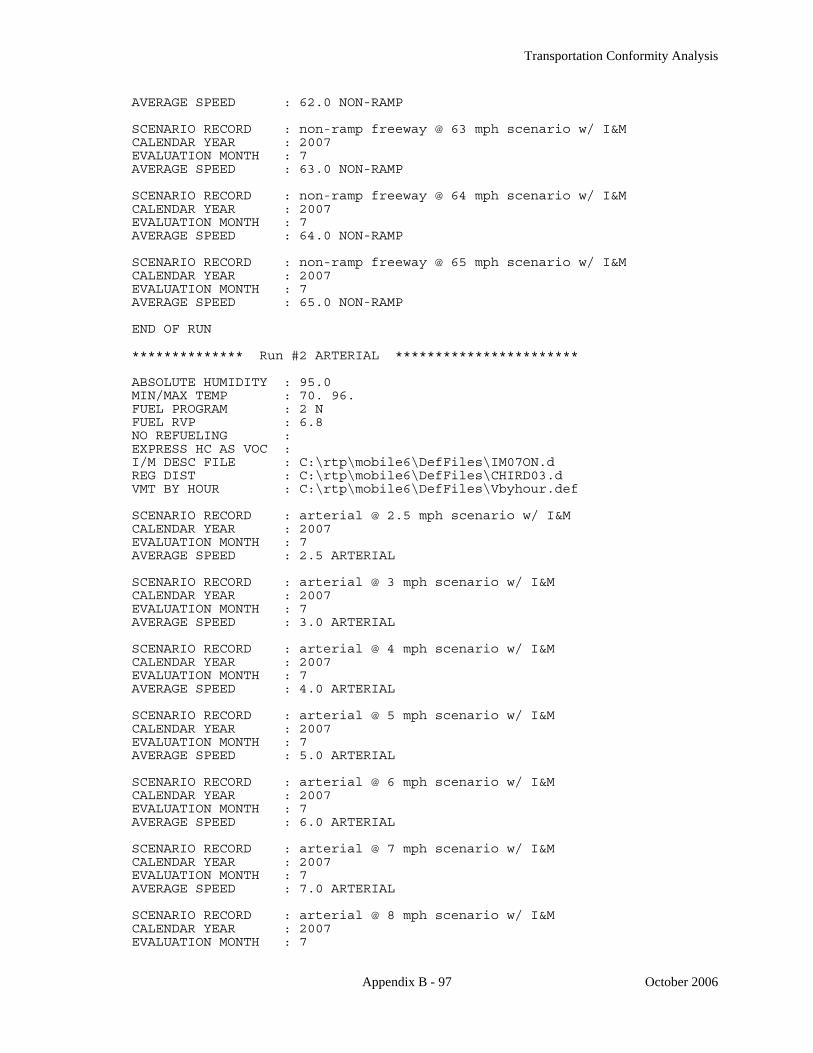
Transportation Conformity Analysis
Appendix B - 97 October 2006
AVERAGE SPEED : 62.0 NON-RAMP SCENARIO RECORD : non-ramp freeway @ 63 mph scenario w/ I&M CALENDAR YEAR : 2007 EVALUATION MONTH : 7 AVERAGE SPEED : 63.0 NON-RAMP SCENARIO RECORD : non-ramp freeway @ 64 mph scenario w/ I&M CALENDAR YEAR : 2007 EVALUATION MONTH : 7 AVERAGE SPEED : 64.0 NON-RAMP SCENARIO RECORD : non-ramp freeway @ 65 mph scenario w/ I&M CALENDAR YEAR : 2007 EVALUATION MONTH : 7 AVERAGE SPEED : 65.0 NON-RAMP END OF RUN ************** Run #2 ARTERIAL *********************** ABSOLUTE HUMIDITY : 95.0 MIN/MAX TEMP : 70. 96. FUEL PROGRAM : 2 N FUEL RVP : 6.8 NO REFUELING : EXPRESS HC AS VOC : I/M DESC FILE : C:\rtp\mobile6\DefFiles\IM07ON.d REG DIST : C:\rtp\mobile6\DefFiles\CHIRD03.d VMT BY HOUR : C:\rtp\mobile6\DefFiles\Vbyhour.def SCENARIO RECORD : arterial @ 2.5 mph scenario w/ I&M CALENDAR YEAR : 2007 EVALUATION MONTH : 7 AVERAGE SPEED : 2.5 ARTERIAL SCENARIO RECORD : arterial @ 3 mph scenario w/ I&M CALENDAR YEAR : 2007 EVALUATION MONTH : 7 AVERAGE SPEED : 3.0 ARTERIAL SCENARIO RECORD : arterial @ 4 mph scenario w/ I&M CALENDAR YEAR : 2007 EVALUATION MONTH : 7 AVERAGE SPEED : 4.0 ARTERIAL SCENARIO RECORD : arterial @ 5 mph scenario w/ I&M CALENDAR YEAR : 2007 EVALUATION MONTH : 7 AVERAGE SPEED : 5.0 ARTERIAL SCENARIO RECORD : arterial @ 6 mph scenario w/ I&M CALENDAR YEAR : 2007 EVALUATION MONTH : 7 AVERAGE SPEED : 6.0 ARTERIAL SCENARIO RECORD : arterial @ 7 mph scenario w/ I&M CALENDAR YEAR : 2007 EVALUATION MONTH : 7 AVERAGE SPEED : 7.0 ARTERIAL SCENARIO RECORD : arterial @ 8 mph scenario w/ I&M CALENDAR YEAR : 2007 EVALUATION MONTH : 7

Transportation Conformity Analysis
Appendix B - 98 October 2006
AVERAGE SPEED : 8.0 ARTERIAL SCENARIO RECORD : arterial @ 9 mph scenario w/ I&M CALENDAR YEAR : 2007 EVALUATION MONTH : 7 AVERAGE SPEED : 9.0 ARTERIAL SCENARIO RECORD : arterial @ 10 mph scenario w/ I&M CALENDAR YEAR : 2007 EVALUATION MONTH : 7 AVERAGE SPEED : 10.0 ARTERIAL SCENARIO RECORD : arterial @ 11 mph scenario w/ I&M CALENDAR YEAR : 2007 EVALUATION MONTH : 7 AVERAGE SPEED : 11.0 ARTERIAL SCENARIO RECORD : arterial @ 12 mph scenario w/ I&M CALENDAR YEAR : 2007 EVALUATION MONTH : 7 AVERAGE SPEED : 12.0 ARTERIAL SCENARIO RECORD : arterial @ 13 mph scenario w/ I&M CALENDAR YEAR : 2007 EVALUATION MONTH : 7 AVERAGE SPEED : 13.0 ARTERIAL SCENARIO RECORD : arterial @ 14 mph scenario w/ I&M CALENDAR YEAR : 2007 EVALUATION MONTH : 7 AVERAGE SPEED : 14.0 ARTERIAL SCENARIO RECORD : arterial @ 15 mph scenario w/ I&M CALENDAR YEAR : 2007 EVALUATION MONTH : 7 AVERAGE SPEED : 15.0 ARTERIAL SCENARIO RECORD : arterial @ 16 mph scenario w/ I&M CALENDAR YEAR : 2007 EVALUATION MONTH : 7 AVERAGE SPEED : 16.0 ARTERIAL SCENARIO RECORD : arterial @ 17 mph scenario w/ I&M CALENDAR YEAR : 2007 EVALUATION MONTH : 7 AVERAGE SPEED : 17.0 ARTERIAL SCENARIO RECORD : arterial @ 18 mph scenario w/ I&M CALENDAR YEAR : 2007 EVALUATION MONTH : 7 AVERAGE SPEED : 18.0 ARTERIAL SCENARIO RECORD : arterial @ 19 mph scenario w/ I&M CALENDAR YEAR : 2007 EVALUATION MONTH : 7 AVERAGE SPEED : 19.0 ARTERIAL SCENARIO RECORD : arterial @ 20 mph scenario w/ I&M CALENDAR YEAR : 2007 EVALUATION MONTH : 7 AVERAGE SPEED : 20.0 ARTERIAL SCENARIO RECORD : arterial @ 21 mph scenario w/ I&M CALENDAR YEAR : 2007

Transportation Conformity Analysis
Appendix B - 99 October 2006
EVALUATION MONTH : 7 AVERAGE SPEED : 21.0 ARTERIAL SCENARIO RECORD : arterial @ 22 mph scenario w/ I&M CALENDAR YEAR : 2007 EVALUATION MONTH : 7 AVERAGE SPEED : 22.0 ARTERIAL SCENARIO RECORD : arterial @ 23 mph scenario w/ I&M CALENDAR YEAR : 2007 EVALUATION MONTH : 7 AVERAGE SPEED : 23.0 ARTERIAL SCENARIO RECORD : arterial @ 24 mph scenario w/ I&M CALENDAR YEAR : 2007 EVALUATION MONTH : 7 AVERAGE SPEED : 24.0 ARTERIAL SCENARIO RECORD : arterial @ 25 mph scenario w/ I&M CALENDAR YEAR : 2007 EVALUATION MONTH : 7 AVERAGE SPEED : 25.0 ARTERIAL SCENARIO RECORD : arterial @ 26 mph scenario w/ I&M CALENDAR YEAR : 2007 EVALUATION MONTH : 7 AVERAGE SPEED : 26.0 ARTERIAL SCENARIO RECORD : arterial @ 27 mph scenario w/ I&M CALENDAR YEAR : 2007 EVALUATION MONTH : 7 AVERAGE SPEED : 27.0 ARTERIAL SCENARIO RECORD : arterial @ 28 mph scenario w/ I&M CALENDAR YEAR : 2007 EVALUATION MONTH : 7 AVERAGE SPEED : 28.0 ARTERIAL SCENARIO RECORD : arterial @ 29 mph scenario w/ I&M CALENDAR YEAR : 2007 EVALUATION MONTH : 7 AVERAGE SPEED : 29.0 ARTERIAL SCENARIO RECORD : arterial @ 30 mph scenario w/ I&M CALENDAR YEAR : 2007 EVALUATION MONTH : 7 AVERAGE SPEED : 30.0 ARTERIAL SCENARIO RECORD : arterial @ 31 mph scenario w/ I&M CALENDAR YEAR : 2007 EVALUATION MONTH : 7 AVERAGE SPEED : 31.0 ARTERIAL SCENARIO RECORD : arterial @ 32 mph scenario w/ I&M CALENDAR YEAR : 2007 EVALUATION MONTH : 7 AVERAGE SPEED : 32.0 ARTERIAL SCENARIO RECORD : arterial @ 33 mph scenario w/ I&M CALENDAR YEAR : 2007 EVALUATION MONTH : 7 AVERAGE SPEED : 33.0 ARTERIAL SCENARIO RECORD : arterial @ 34 mph scenario w/ I&M
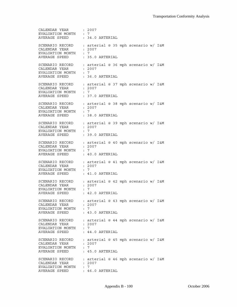
Transportation Conformity Analysis
Appendix B - 100 October 2006
CALENDAR YEAR : 2007 EVALUATION MONTH : 7 AVERAGE SPEED : 34.0 ARTERIAL SCENARIO RECORD : arterial @ 35 mph scenario w/ I&M CALENDAR YEAR : 2007 EVALUATION MONTH : 7 AVERAGE SPEED : 35.0 ARTERIAL SCENARIO RECORD : arterial @ 36 mph scenario w/ I&M CALENDAR YEAR : 2007 EVALUATION MONTH : 7 AVERAGE SPEED : 36.0 ARTERIAL SCENARIO RECORD : arterial @ 37 mph scenario w/ I&M CALENDAR YEAR : 2007 EVALUATION MONTH : 7 AVERAGE SPEED : 37.0 ARTERIAL SCENARIO RECORD : arterial @ 38 mph scenario w/ I&M CALENDAR YEAR : 2007 EVALUATION MONTH : 7 AVERAGE SPEED : 38.0 ARTERIAL SCENARIO RECORD : arterial @ 39 mph scenario w/ I&M CALENDAR YEAR : 2007 EVALUATION MONTH : 7 AVERAGE SPEED : 39.0 ARTERIAL SCENARIO RECORD : arterial @ 40 mph scenario w/ I&M CALENDAR YEAR : 2007 EVALUATION MONTH : 7 AVERAGE SPEED : 40.0 ARTERIAL SCENARIO RECORD : arterial @ 41 mph scenario w/ I&M CALENDAR YEAR : 2007 EVALUATION MONTH : 7 AVERAGE SPEED : 41.0 ARTERIAL SCENARIO RECORD : arterial @ 42 mph scenario w/ I&M CALENDAR YEAR : 2007 EVALUATION MONTH : 7 AVERAGE SPEED : 42.0 ARTERIAL SCENARIO RECORD : arterial @ 43 mph scenario w/ I&M CALENDAR YEAR : 2007 EVALUATION MONTH : 7 AVERAGE SPEED : 43.0 ARTERIAL SCENARIO RECORD : arterial @ 44 mph scenario w/ I&M CALENDAR YEAR : 2007 EVALUATION MONTH : 7 AVERAGE SPEED : 44.0 ARTERIAL SCENARIO RECORD : arterial @ 45 mph scenario w/ I&M CALENDAR YEAR : 2007 EVALUATION MONTH : 7 AVERAGE SPEED : 45.0 ARTERIAL SCENARIO RECORD : arterial @ 46 mph scenario w/ I&M CALENDAR YEAR : 2007 EVALUATION MONTH : 7 AVERAGE SPEED : 46.0 ARTERIAL

Transportation Conformity Analysis
Appendix B - 101 October 2006
SCENARIO RECORD : arterial @ 47 mph scenario w/ I&M CALENDAR YEAR : 2007 EVALUATION MONTH : 7 AVERAGE SPEED : 47.0 ARTERIAL SCENARIO RECORD : arterial @ 48 mph scenario w/ I&M CALENDAR YEAR : 2007 EVALUATION MONTH : 7 AVERAGE SPEED : 48.0 ARTERIAL SCENARIO RECORD : arterial @ 49 mph scenario w/ I&M CALENDAR YEAR : 2007 EVALUATION MONTH : 7 AVERAGE SPEED : 49.0 ARTERIAL SCENARIO RECORD : arterial @ 50 mph scenario w/ I&M CALENDAR YEAR : 2007 EVALUATION MONTH : 7 AVERAGE SPEED : 50.0 ARTERIAL SCENARIO RECORD : arterial @ 51 mph scenario w/ I&M CALENDAR YEAR : 2007 EVALUATION MONTH : 7 AVERAGE SPEED : 51.0 ARTERIAL SCENARIO RECORD : arterial @ 52 mph scenario w/ I&M CALENDAR YEAR : 2007 EVALUATION MONTH : 7 AVERAGE SPEED : 52.0 ARTERIAL SCENARIO RECORD : arterial @ 53 mph scenario w/ I&M CALENDAR YEAR : 2007 EVALUATION MONTH : 7 AVERAGE SPEED : 53.0 ARTERIAL SCENARIO RECORD : arterial @ 54 mph scenario w/ I&M CALENDAR YEAR : 2007 EVALUATION MONTH : 7 AVERAGE SPEED : 54.0 ARTERIAL SCENARIO RECORD : arterial @ 55 mph scenario w/ I&M CALENDAR YEAR : 2007 EVALUATION MONTH : 7 AVERAGE SPEED : 55.0 ARTERIAL SCENARIO RECORD : arterial @ 56 mph scenario w/ I&M CALENDAR YEAR : 2007 EVALUATION MONTH : 7 AVERAGE SPEED : 56.0 ARTERIAL SCENARIO RECORD : arterial @ 57 mph scenario w/ I&M CALENDAR YEAR : 2007 EVALUATION MONTH : 7 AVERAGE SPEED : 57.0 ARTERIAL SCENARIO RECORD : arterial @ 58 mph scenario w/ I&M CALENDAR YEAR : 2007 EVALUATION MONTH : 7 AVERAGE SPEED : 58.0 ARTERIAL SCENARIO RECORD : arterial @ 59 mph scenario w/ I&M CALENDAR YEAR : 2007 EVALUATION MONTH : 7 AVERAGE SPEED : 59.0 ARTERIAL

Transportation Conformity Analysis
Appendix B - 102 October 2006
SCENARIO RECORD : arterial @ 60 mph scenario w/ I&M CALENDAR YEAR : 2007 EVALUATION MONTH : 7 AVERAGE SPEED : 60.0 ARTERIAL SCENARIO RECORD : arterial @ 61 mph scenario w/ I&M CALENDAR YEAR : 2007 EVALUATION MONTH : 7 AVERAGE SPEED : 61.0 ARTERIAL SCENARIO RECORD : arterial @ 62 mph scenario w/ I&M CALENDAR YEAR : 2007 EVALUATION MONTH : 7 AVERAGE SPEED : 62.0 ARTERIAL SCENARIO RECORD : arterial @ 63 mph scenario w/ I&M CALENDAR YEAR : 2007 EVALUATION MONTH : 7 AVERAGE SPEED : 63.0 ARTERIAL SCENARIO RECORD : arterial @ 64 mph scenario w/ I&M CALENDAR YEAR : 2007 EVALUATION MONTH : 7 AVERAGE SPEED : 64.0 ARTERIAL SCENARIO RECORD : arterial @ 65 mph scenario w/ I&M CALENDAR YEAR : 2007 EVALUATION MONTH : 7 AVERAGE SPEED : 65.0 ARTERIAL END OF RUN ************** Run #3 LOCAL *********************** ABSOLUTE HUMIDITY : 95.0 MIN/MAX TEMP : 70. 96. FUEL PROGRAM : 2 N FUEL RVP : 6.8 NO REFUELING : EXPRESS HC AS VOC : I/M DESC FILE : C:\rtp\mobile6\DefFiles\IM07ON.d REG DIST : C:\rtp\mobile6\DefFiles\CHIRD03.d VMT BY HOUR : C:\rtp\mobile6\DefFiles\Vbyhour.def VMT BY FACILITY : C:\rtp\mobile6\DefFiles\FVMTLCL.d SCENARIO RECORD : local vmt only w/ I&M CALENDAR YEAR : 2007 EVALUATION MONTH : 7 END OF RUN ************** Run #4 RAMP *********************** ABSOLUTE HUMIDITY : 95.0 MIN/MAX TEMP : 70. 96. FUEL PROGRAM : 2 N FUEL RVP : 6.8 NO REFUELING : EXPRESS HC AS VOC : I/M DESC FILE : C:\rtp\mobile6\DefFiles\IM07ON.d REG DIST : C:\rtp\mobile6\DefFiles\CHIRD03.d VMT BY HOUR : C:\rtp\mobile6\DefFiles\Vbyhour.def VMT BY FACILITY : C:\rtp\mobile6\DefFiles\FVMTRMP.def

Transportation Conformity Analysis
Appendix B - 103 October 2006
SCENARIO RECORD : ramp vmt only w/ I&M CALENDAR YEAR : 2007 EVALUATION MONTH : 7 END OF RUN
Input values The input values used are described below: POLLUTANTS : HC NOX
This instructs MOBILE6 to report emission rates for hydrocarbons and oxides of nitrogen, the two regulated ozone precursors in the region. REPORT FILE : C:\rtp\mobile6\ozone\rates07.txt
The general log file, listing input commands, warnings, and error messages is put in this file SPREADSHEET : C:\rtp\mobile6\ozone\rates07.tab
The emission rates are put in this file in a format suitable for importing into a spreadsheet. ABSOLUTE HUMIDITY : 95.0
Humidity affects emission rates; MOBILE6 requires an absolute humidity input (in grains per pound). This value was developed using relative humidity data at O’Hare International Airport from the ten highest ozone days in the 1988 to 1990 period. These same data were used in the Chicago 1990 inventory, the 15 Percent and 9 Percent Rate of Progress Plans, the Attainment Demonstration, the current SIP, and previous conformity analyses. The method was developed by the U.S. Environmental Protection Agency, and applied by the Illinois Environmental Protection Agency. MIN/MAX TEMP : 70. 96.
MOBILE6 requires the maximum and minimum temperature to calculate emission rates. These values were developed using data at O’Hare International Airport from the ten highest ozone days in the 1988 to 1990 period. These same data were used in the Chicago 1990 inventory, the 15 Percent and 9 Percent Rate of Progress Plans, the Attainment Demonstration, the current SIP, and previous conformity analyses. FUEL PROGRAM : 2 N
This input specifies that reformulated gasoline for northern states will be used in the region during the period for which emission rates are being calculated. This is consistent with values used in the SIP. In the Fall of 2005, USEPA announced that MOBILE6 has an error whereby specifying a fuel program results in summer fuel sulfur levels being applied to winter months as well, rather than using the default higher winter sulfur levels. For years after 2007, winter and summer sulfur levels will be the same, and the error has no effect. This is the case for analysis years 2010, 2020 and 2030. The 2007 analysis year only applies to ozone conformity, so the analysis is for the summer, and the error again has no effect. The 2002 baseline year for PM2.5 conformity is affected by the error. The nature of the error is to underestimate particulate and NOx emissions, so in fact the baseline values for these emissions are understated. Since emissions for the analysis years of 2010, 2020 and 2030 are all less than the understated baseline emissions, they are also less than the unknown, but higher, baseline emissions that would result from correcting winter sulfur levels. Because the correction would not affect the analysis, the baseline emissions have not been recalculated.

Transportation Conformity Analysis
Appendix B - 104 October 2006
FUEL RVP : 6.8
MOBILE6 requires the refueling Reid vapor pressure (in pounds per square inch) to determine the effect of fuel volatility on emissions. This value derives from the fuel program in place, based on the table on page 151 of User’s Guide to MOBILE6.1 and MOBILE6.2: Mobile Source Emissions Factor Model. NO REFUELING :
No emissions due to refueling are included in the emission rates. In the SIP, these are treated as area emissions, not mobile emissions. EXPRESS HC AS VOC :
The hydrocarbon emissions are expressed in terms of volatile organic compounds. I/M DESC FILE : C:\rtp\mobile6\DefFiles\IM07ON.d
This is the file which defines the inspection and maintenance program. It is discussed further in a following section. REG DIST : C:\rtp\mobile6\DefFiles\CHIRD03.d
This is the file which defines the vehicle age distribution. It is discussed further in a following section. VMT BY HOUR : C:\rtp\mobile6\DefFiles\Vbyhour.def
This is the file which defines the distribution of VMT by hour of the day. It is discussed further in a following section. SCENARIO RECORD : non-ramp freeway @ 2.5 mph scenario w/ I&M
This record is simply a header record for each scenario section. The text to the right of the colon is placed in the output as a descriptive field. CALENDAR YEAR : 2007
The emission rates are generated for 2007. EVALUATION MONTH : 7
The emission rates generated are for the month of July, which is the standard month for generating emission rates for ozone precursors. The alternative month, January, is not applicable. AVERAGE SPEED : 2.5 NON-RAMP
The emission rates generated by this scenario assume that all vehicles travel at 2.5 mph on a freeway (not the ramp). A scenario is run for each mile per hour from 2.5 through 65 on the freeway and from 2.5 mph to 65 mph on arterial streets, to match the VMT at each speed and facility. One additional scenario is run for local streets and one for freeway ramps; these facilities use only one speed in the MOBILE6 model. VMT BY FACILITY : C:\rtp\mobile6\DefFiles\FVMTRMP.def VMT BY FACILITY : C:\rtp\mobile6\DefFiles\FVMTLCL.d
These two commands are used to specify that emission rates are to be generated as though all VMT are on local streets (FVMTLCL.d) or freeway ramps (FVMTRMP.def). For arterials and freeways, the AVERAGE SPEED command accomplishes the same thing.
8.4.1.2 PM2.5 Conformity – Direct PM2.5
The following listing shows the input for obtaining the direct PM2.5 emission rates for the 2010 scenario year for the months January - March. A similar file was used to generate emission rates for the other months of the year, and for the other scenario years. Most of the input values have been described in the previous section on the ozone MOBILE runs; a description of the input values unique to PM2.5 follows the listing.
************************************************************************* * * * DESCRIPTION: PM emission rates for facilities & speeds individually *
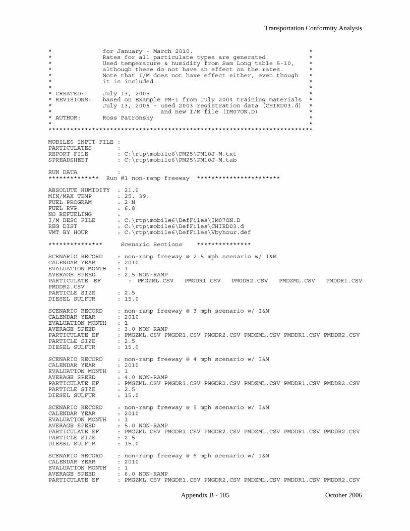
Transportation Conformity Analysis
Appendix B - 105 October 2006
* for January - March 2010. * * Rates for all particulate types are generated * * Used temperature & humidity from Sam Long table 5-10, * * although these do not have an effect on the rates. * * Note that I/M does not have effect either, even though * * it is included. * * * * CREATED: July 13, 2005 * * REVISIONS: based on Example PM-1 from July 2004 training materials * * July 13, 2006 - used 2003 registration data (CHIRD03.d) * * and new I/M file (IM07ON.D) * * AUTHOR: Ross Patronsky * * * ************************************************************************* MOBILE6 INPUT FILE : PARTICULATES : REPORT FILE : C:\rtp\mobile6\PM25\PM10J-M.txt SPREADSHEET : C:\rtp\mobile6\PM25\PM10J-M.tab RUN DATA : ************** Run #1 non-ramp freeway *********************** ABSOLUTE HUMIDITY : 21.0 MIN/MAX TEMP : 25. 39. FUEL PROGRAM : 2 N FUEL RVP : 6.8 NO REFUELING : I/M DESC FILE : C:\rtp\mobile6\DefFiles\IM07ON.D REG DIST : C:\rtp\mobile6\DefFiles\CHIRD03.d VMT BY HOUR : C:\rtp\mobile6\DefFiles\Vbyhour.def *************** Scenario Sections *************** SCENARIO RECORD : non-ramp freeway @ 2.5 mph scenario w/ I&M CALENDAR YEAR : 2010 EVALUATION MONTH : 1 AVERAGE SPEED : 2.5 NON-RAMP PARTICULATE EF : PMGZML.CSV PMGDR1.CSV PMGDR2.CSV PMDZML.CSV PMDDR1.CSV PMDDR2.CSV PARTICLE SIZE : 2.5 DIESEL SULFUR : 15.0 SCENARIO RECORD : non-ramp freeway @ 3 mph scenario w/ I&M CALENDAR YEAR : 2010 EVALUATION MONTH : 1 AVERAGE SPEED : 3.0 NON-RAMP PARTICULATE EF : PMGZML.CSV PMGDR1.CSV PMGDR2.CSV PMDZML.CSV PMDDR1.CSV PMDDR2.CSV PARTICLE SIZE : 2.5 DIESEL SULFUR : 15.0 SCENARIO RECORD : non-ramp freeway @ 4 mph scenario w/ I&M CALENDAR YEAR : 2010 EVALUATION MONTH : 1 AVERAGE SPEED : 4.0 NON-RAMP PARTICULATE EF : PMGZML.CSV PMGDR1.CSV PMGDR2.CSV PMDZML.CSV PMDDR1.CSV PMDDR2.CSV PARTICLE SIZE : 2.5 DIESEL SULFUR : 15.0 SCENARIO RECORD : non-ramp freeway @ 5 mph scenario w/ I&M CALENDAR YEAR : 2010 EVALUATION MONTH : 1 AVERAGE SPEED : 5.0 NON-RAMP PARTICULATE EF : PMGZML.CSV PMGDR1.CSV PMGDR2.CSV PMDZML.CSV PMDDR1.CSV PMDDR2.CSV PARTICLE SIZE : 2.5 DIESEL SULFUR : 15.0 SCENARIO RECORD : non-ramp freeway @ 6 mph scenario w/ I&M CALENDAR YEAR : 2010 EVALUATION MONTH : 1 AVERAGE SPEED : 6.0 NON-RAMP PARTICULATE EF : PMGZML.CSV PMGDR1.CSV PMGDR2.CSV PMDZML.CSV PMDDR1.CSV PMDDR2.CSV

Transportation Conformity Analysis
Appendix B - 106 October 2006
PARTICLE SIZE : 2.5 DIESEL SULFUR : 15.0 SCENARIO RECORD : non-ramp freeway @ 7 mph scenario w/ I&M CALENDAR YEAR : 2010 EVALUATION MONTH : 1 AVERAGE SPEED : 7.0 NON-RAMP PARTICULATE EF : PMGZML.CSV PMGDR1.CSV PMGDR2.CSV PMDZML.CSV PMDDR1.CSV PMDDR2.CSV PARTICLE SIZE : 2.5 DIESEL SULFUR : 15.0 SCENARIO RECORD : non-ramp freeway @ 8 mph scenario w/ I&M CALENDAR YEAR : 2010 EVALUATION MONTH : 1 AVERAGE SPEED : 8.0 NON-RAMP PARTICULATE EF : PMGZML.CSV PMGDR1.CSV PMGDR2.CSV PMDZML.CSV PMDDR1.CSV PMDDR2.CSV PARTICLE SIZE : 2.5 DIESEL SULFUR : 15.0 SCENARIO RECORD : non-ramp freeway @ 9 mph scenario w/ I&M CALENDAR YEAR : 2010 EVALUATION MONTH : 1 AVERAGE SPEED : 9.0 NON-RAMP PARTICULATE EF : PMGZML.CSV PMGDR1.CSV PMGDR2.CSV PMDZML.CSV PMDDR1.CSV PMDDR2.CSV PARTICLE SIZE : 2.5 DIESEL SULFUR : 15.0 SCENARIO RECORD : non-ramp freeway @ 10 mph scenario w/ I&M CALENDAR YEAR : 2010 EVALUATION MONTH : 1 AVERAGE SPEED : 10.0 NON-RAMP PARTICULATE EF : PMGZML.CSV PMGDR1.CSV PMGDR2.CSV PMDZML.CSV PMDDR1.CSV PMDDR2.CSV PARTICLE SIZE : 2.5 DIESEL SULFUR : 15.0 SCENARIO RECORD : non-ramp freeway @ 11 mph scenario w/ I&M CALENDAR YEAR : 2010 EVALUATION MONTH : 1 AVERAGE SPEED : 11.0 NON-RAMP PARTICULATE EF : PMGZML.CSV PMGDR1.CSV PMGDR2.CSV PMDZML.CSV PMDDR1.CSV PMDDR2.CSV PARTICLE SIZE : 2.5 DIESEL SULFUR : 15.0 SCENARIO RECORD : non-ramp freeway @ 12 mph scenario w/ I&M CALENDAR YEAR : 2010 EVALUATION MONTH : 1 AVERAGE SPEED : 12.0 NON-RAMP PARTICULATE EF : PMGZML.CSV PMGDR1.CSV PMGDR2.CSV PMDZML.CSV PMDDR1.CSV PMDDR2.CSV PARTICLE SIZE : 2.5 DIESEL SULFUR : 15.0 SCENARIO RECORD : non-ramp freeway @ 13 mph scenario w/ I&M CALENDAR YEAR : 2010 EVALUATION MONTH : 1 AVERAGE SPEED : 13.0 NON-RAMP PARTICULATE EF : PMGZML.CSV PMGDR1.CSV PMGDR2.CSV PMDZML.CSV PMDDR1.CSV PMDDR2.CSV PARTICLE SIZE : 2.5 DIESEL SULFUR : 15.0 SCENARIO RECORD : non-ramp freeway @ 14 mph scenario w/ I&M CALENDAR YEAR : 2010 EVALUATION MONTH : 1 AVERAGE SPEED : 14.0 NON-RAMP PARTICULATE EF : PMGZML.CSV PMGDR1.CSV PMGDR2.CSV PMDZML.CSV PMDDR1.CSV PMDDR2.CSV PARTICLE SIZE : 2.5 DIESEL SULFUR : 15.0 SCENARIO RECORD : non-ramp freeway @ 15 mph scenario w/ I&M CALENDAR YEAR : 2010 EVALUATION MONTH : 1 AVERAGE SPEED : 15.0 NON-RAMP PARTICULATE EF : PMGZML.CSV PMGDR1.CSV PMGDR2.CSV PMDZML.CSV PMDDR1.CSV PMDDR2.CSV

Transportation Conformity Analysis
Appendix B - 107 October 2006
PARTICLE SIZE : 2.5 DIESEL SULFUR : 15.0 SCENARIO RECORD : non-ramp freeway @ 16 mph scenario w/ I&M CALENDAR YEAR : 2010 EVALUATION MONTH : 1 AVERAGE SPEED : 16.0 NON-RAMP PARTICULATE EF : PMGZML.CSV PMGDR1.CSV PMGDR2.CSV PMDZML.CSV PMDDR1.CSV PMDDR2.CSV PARTICLE SIZE : 2.5 DIESEL SULFUR : 15.0 SCENARIO RECORD : non-ramp freeway @ 17 mph scenario w/ I&M CALENDAR YEAR : 2010 EVALUATION MONTH : 1 AVERAGE SPEED : 17.0 NON-RAMP PARTICULATE EF : PMGZML.CSV PMGDR1.CSV PMGDR2.CSV PMDZML.CSV PMDDR1.CSV PMDDR2.CSV PARTICLE SIZE : 2.5 DIESEL SULFUR : 15.0 SCENARIO RECORD : non-ramp freeway @ 18 mph scenario w/ I&M CALENDAR YEAR : 2010 EVALUATION MONTH : 1 AVERAGE SPEED : 18.0 NON-RAMP PARTICULATE EF : PMGZML.CSV PMGDR1.CSV PMGDR2.CSV PMDZML.CSV PMDDR1.CSV PMDDR2.CSV PARTICLE SIZE : 2.5 DIESEL SULFUR : 15.0 SCENARIO RECORD : non-ramp freeway @ 19 mph scenario w/ I&M CALENDAR YEAR : 2010 EVALUATION MONTH : 1 AVERAGE SPEED : 19.0 NON-RAMP PARTICULATE EF : PMGZML.CSV PMGDR1.CSV PMGDR2.CSV PMDZML.CSV PMDDR1.CSV PMDDR2.CSV PARTICLE SIZE : 2.5 DIESEL SULFUR : 15.0 SCENARIO RECORD : non-ramp freeway @ 20 mph scenario w/ I&M CALENDAR YEAR : 2010 EVALUATION MONTH : 1 AVERAGE SPEED : 20.0 NON-RAMP PARTICULATE EF : PMGZML.CSV PMGDR1.CSV PMGDR2.CSV PMDZML.CSV PMDDR1.CSV PMDDR2.CSV PARTICLE SIZE : 2.5 DIESEL SULFUR : 15.0 SCENARIO RECORD : non-ramp freeway @ 21 mph scenario w/ I&M CALENDAR YEAR : 2010 EVALUATION MONTH : 1 AVERAGE SPEED : 21.0 NON-RAMP PARTICULATE EF : PMGZML.CSV PMGDR1.CSV PMGDR2.CSV PMDZML.CSV PMDDR1.CSV PMDDR2.CSV PARTICLE SIZE : 2.5 DIESEL SULFUR : 15.0 SCENARIO RECORD : non-ramp freeway @ 22 mph scenario w/ I&M CALENDAR YEAR : 2010 EVALUATION MONTH : 1 AVERAGE SPEED : 22.0 NON-RAMP PARTICULATE EF : PMGZML.CSV PMGDR1.CSV PMGDR2.CSV PMDZML.CSV PMDDR1.CSV PMDDR2.CSV PARTICLE SIZE : 2.5 DIESEL SULFUR : 15.0 SCENARIO RECORD : non-ramp freeway @ 23 mph scenario w/ I&M CALENDAR YEAR : 2010 EVALUATION MONTH : 1 AVERAGE SPEED : 23.0 NON-RAMP PARTICULATE EF : PMGZML.CSV PMGDR1.CSV PMGDR2.CSV PMDZML.CSV PMDDR1.CSV PMDDR2.CSV PARTICLE SIZE : 2.5 DIESEL SULFUR : 15.0 SCENARIO RECORD : non-ramp freeway @ 24 mph scenario w/ I&M CALENDAR YEAR : 2010 EVALUATION MONTH : 1 AVERAGE SPEED : 24.0 NON-RAMP PARTICULATE EF : PMGZML.CSV PMGDR1.CSV PMGDR2.CSV PMDZML.CSV PMDDR1.CSV PMDDR2.CSV

Transportation Conformity Analysis
Appendix B - 108 October 2006
PARTICLE SIZE : 2.5 DIESEL SULFUR : 15.0 SCENARIO RECORD : non-ramp freeway @ 25 mph scenario w/ I&M CALENDAR YEAR : 2010 EVALUATION MONTH : 1 AVERAGE SPEED : 25.0 NON-RAMP PARTICULATE EF : PMGZML.CSV PMGDR1.CSV PMGDR2.CSV PMDZML.CSV PMDDR1.CSV PMDDR2.CSV PARTICLE SIZE : 2.5 DIESEL SULFUR : 15.0 SCENARIO RECORD : non-ramp freeway @ 26 mph scenario w/ I&M CALENDAR YEAR : 2010 EVALUATION MONTH : 1 AVERAGE SPEED : 26.0 NON-RAMP PARTICULATE EF : PMGZML.CSV PMGDR1.CSV PMGDR2.CSV PMDZML.CSV PMDDR1.CSV PMDDR2.CSV PARTICLE SIZE : 2.5 DIESEL SULFUR : 15.0 SCENARIO RECORD : non-ramp freeway @ 27 mph scenario w/ I&M CALENDAR YEAR : 2010 EVALUATION MONTH : 1 AVERAGE SPEED : 27.0 NON-RAMP PARTICULATE EF : PMGZML.CSV PMGDR1.CSV PMGDR2.CSV PMDZML.CSV PMDDR1.CSV PMDDR2.CSV PARTICLE SIZE : 2.5 DIESEL SULFUR : 15.0 SCENARIO RECORD : non-ramp freeway @ 28 mph scenario w/ I&M CALENDAR YEAR : 2010 EVALUATION MONTH : 1 AVERAGE SPEED : 28.0 NON-RAMP PARTICULATE EF : PMGZML.CSV PMGDR1.CSV PMGDR2.CSV PMDZML.CSV PMDDR1.CSV PMDDR2.CSV PARTICLE SIZE : 2.5 DIESEL SULFUR : 15.0 SCENARIO RECORD : non-ramp freeway @ 29 mph scenario w/ I&M CALENDAR YEAR : 2010 EVALUATION MONTH : 1 AVERAGE SPEED : 29.0 NON-RAMP PARTICULATE EF : PMGZML.CSV PMGDR1.CSV PMGDR2.CSV PMDZML.CSV PMDDR1.CSV PMDDR2.CSV PARTICLE SIZE : 2.5 DIESEL SULFUR : 15.0 SCENARIO RECORD : non-ramp freeway @ 30 mph scenario w/ I&M CALENDAR YEAR : 2010 EVALUATION MONTH : 1 AVERAGE SPEED : 30.0 NON-RAMP PARTICULATE EF : PMGZML.CSV PMGDR1.CSV PMGDR2.CSV PMDZML.CSV PMDDR1.CSV PMDDR2.CSV PARTICLE SIZE : 2.5 DIESEL SULFUR : 15.0 SCENARIO RECORD : non-ramp freeway @ 31 mph scenario w/ I&M CALENDAR YEAR : 2010 EVALUATION MONTH : 1 AVERAGE SPEED : 31.0 NON-RAMP PARTICULATE EF : PMGZML.CSV PMGDR1.CSV PMGDR2.CSV PMDZML.CSV PMDDR1.CSV PMDDR2.CSV PARTICLE SIZE : 2.5 DIESEL SULFUR : 15.0 SCENARIO RECORD : non-ramp freeway @ 32 mph scenario w/ I&M CALENDAR YEAR : 2010 EVALUATION MONTH : 1 AVERAGE SPEED : 32.0 NON-RAMP PARTICULATE EF : PMGZML.CSV PMGDR1.CSV PMGDR2.CSV PMDZML.CSV PMDDR1.CSV PMDDR2.CSV PARTICLE SIZE : 2.5 DIESEL SULFUR : 15.0 SCENARIO RECORD : non-ramp freeway @ 33 mph scenario w/ I&M CALENDAR YEAR : 2010 EVALUATION MONTH : 1 AVERAGE SPEED : 33.0 NON-RAMP PARTICULATE EF : PMGZML.CSV PMGDR1.CSV PMGDR2.CSV PMDZML.CSV PMDDR1.CSV PMDDR2.CSV

Transportation Conformity Analysis
Appendix B - 109 October 2006
PARTICLE SIZE : 2.5 DIESEL SULFUR : 15.0 SCENARIO RECORD : non-ramp freeway @ 34 mph scenario w/ I&M CALENDAR YEAR : 2010 EVALUATION MONTH : 1 AVERAGE SPEED : 34.0 NON-RAMP PARTICULATE EF : PMGZML.CSV PMGDR1.CSV PMGDR2.CSV PMDZML.CSV PMDDR1.CSV PMDDR2.CSV PARTICLE SIZE : 2.5 DIESEL SULFUR : 15.0 SCENARIO RECORD : non-ramp freeway @ 35 mph scenario w/ I&M CALENDAR YEAR : 2010 EVALUATION MONTH : 1 AVERAGE SPEED : 35.0 NON-RAMP PARTICULATE EF : PMGZML.CSV PMGDR1.CSV PMGDR2.CSV PMDZML.CSV PMDDR1.CSV PMDDR2.CSV PARTICLE SIZE : 2.5 DIESEL SULFUR : 15.0 SCENARIO RECORD : non-ramp freeway @ 36 mph scenario w/ I&M CALENDAR YEAR : 2010 EVALUATION MONTH : 1 AVERAGE SPEED : 36.0 NON-RAMP PARTICULATE EF : PMGZML.CSV PMGDR1.CSV PMGDR2.CSV PMDZML.CSV PMDDR1.CSV PMDDR2.CSV PARTICLE SIZE : 2.5 DIESEL SULFUR : 15.0 SCENARIO RECORD : non-ramp freeway @ 37 mph scenario w/ I&M CALENDAR YEAR : 2010 EVALUATION MONTH : 1 AVERAGE SPEED : 37.0 NON-RAMP PARTICULATE EF : PMGZML.CSV PMGDR1.CSV PMGDR2.CSV PMDZML.CSV PMDDR1.CSV PMDDR2.CSV PARTICLE SIZE : 2.5 DIESEL SULFUR : 15.0 SCENARIO RECORD : non-ramp freeway @ 38 mph scenario w/ I&M CALENDAR YEAR : 2010 EVALUATION MONTH : 1 AVERAGE SPEED : 38.0 NON-RAMP PARTICULATE EF : PMGZML.CSV PMGDR1.CSV PMGDR2.CSV PMDZML.CSV PMDDR1.CSV PMDDR2.CSV PARTICLE SIZE : 2.5 DIESEL SULFUR : 15.0 SCENARIO RECORD : non-ramp freeway @ 39 mph scenario w/ I&M CALENDAR YEAR : 2010 EVALUATION MONTH : 1 AVERAGE SPEED : 39.0 NON-RAMP PARTICULATE EF : PMGZML.CSV PMGDR1.CSV PMGDR2.CSV PMDZML.CSV PMDDR1.CSV PMDDR2.CSV PARTICLE SIZE : 2.5 DIESEL SULFUR : 15.0 SCENARIO RECORD : non-ramp freeway @ 40 mph scenario w/ I&M CALENDAR YEAR : 2010 EVALUATION MONTH : 1 AVERAGE SPEED : 40.0 NON-RAMP PARTICULATE EF : PMGZML.CSV PMGDR1.CSV PMGDR2.CSV PMDZML.CSV PMDDR1.CSV PMDDR2.CSV PARTICLE SIZE : 2.5 DIESEL SULFUR : 15.0 SCENARIO RECORD : non-ramp freeway @ 41 mph scenario w/ I&M CALENDAR YEAR : 2010 EVALUATION MONTH : 1 AVERAGE SPEED : 41.0 NON-RAMP PARTICULATE EF : PMGZML.CSV PMGDR1.CSV PMGDR2.CSV PMDZML.CSV PMDDR1.CSV PMDDR2.CSV PARTICLE SIZE : 2.5 DIESEL SULFUR : 15.0 SCENARIO RECORD : non-ramp freeway @ 42 mph scenario w/ I&M CALENDAR YEAR : 2010 EVALUATION MONTH : 1 AVERAGE SPEED : 42.0 NON-RAMP PARTICULATE EF : PMGZML.CSV PMGDR1.CSV PMGDR2.CSV PMDZML.CSV PMDDR1.CSV PMDDR2.CSV

Transportation Conformity Analysis
Appendix B - 110 October 2006
PARTICLE SIZE : 2.5 DIESEL SULFUR : 15.0 SCENARIO RECORD : non-ramp freeway @ 43 mph scenario w/ I&M CALENDAR YEAR : 2010 EVALUATION MONTH : 1 AVERAGE SPEED : 43.0 NON-RAMP PARTICULATE EF : PMGZML.CSV PMGDR1.CSV PMGDR2.CSV PMDZML.CSV PMDDR1.CSV PMDDR2.CSV PARTICLE SIZE : 2.5 DIESEL SULFUR : 15.0 SCENARIO RECORD : non-ramp freeway @ 44 mph scenario w/ I&M CALENDAR YEAR : 2010 EVALUATION MONTH : 1 AVERAGE SPEED : 44.0 NON-RAMP PARTICULATE EF : PMGZML.CSV PMGDR1.CSV PMGDR2.CSV PMDZML.CSV PMDDR1.CSV PMDDR2.CSV PARTICLE SIZE : 2.5 DIESEL SULFUR : 15.0 SCENARIO RECORD : non-ramp freeway @ 45 mph scenario w/ I&M CALENDAR YEAR : 2010 EVALUATION MONTH : 1 AVERAGE SPEED : 45.0 NON-RAMP PARTICULATE EF : PMGZML.CSV PMGDR1.CSV PMGDR2.CSV PMDZML.CSV PMDDR1.CSV PMDDR2.CSV PARTICLE SIZE : 2.5 DIESEL SULFUR : 15.0 SCENARIO RECORD : non-ramp freeway @ 46 mph scenario w/ I&M CALENDAR YEAR : 2010 EVALUATION MONTH : 1 AVERAGE SPEED : 46.0 NON-RAMP PARTICULATE EF : PMGZML.CSV PMGDR1.CSV PMGDR2.CSV PMDZML.CSV PMDDR1.CSV PMDDR2.CSV PARTICLE SIZE : 2.5 DIESEL SULFUR : 15.0 SCENARIO RECORD : non-ramp freeway @ 47 mph scenario w/ I&M CALENDAR YEAR : 2010 EVALUATION MONTH : 1 AVERAGE SPEED : 47.0 NON-RAMP PARTICULATE EF : PMGZML.CSV PMGDR1.CSV PMGDR2.CSV PMDZML.CSV PMDDR1.CSV PMDDR2.CSV PARTICLE SIZE : 2.5 DIESEL SULFUR : 15.0 SCENARIO RECORD : non-ramp freeway @ 48 mph scenario w/ I&M CALENDAR YEAR : 2010 EVALUATION MONTH : 1 AVERAGE SPEED : 48.0 NON-RAMP PARTICULATE EF : PMGZML.CSV PMGDR1.CSV PMGDR2.CSV PMDZML.CSV PMDDR1.CSV PMDDR2.CSV PARTICLE SIZE : 2.5 DIESEL SULFUR : 15.0 SCENARIO RECORD : non-ramp freeway @ 49 mph scenario w/ I&M CALENDAR YEAR : 2010 EVALUATION MONTH : 1 AVERAGE SPEED : 49.0 NON-RAMP PARTICULATE EF : PMGZML.CSV PMGDR1.CSV PMGDR2.CSV PMDZML.CSV PMDDR1.CSV PMDDR2.CSV PARTICLE SIZE : 2.5 DIESEL SULFUR : 15.0 SCENARIO RECORD : non-ramp freeway @ 50 mph scenario w/ I&M CALENDAR YEAR : 2010 EVALUATION MONTH : 1 AVERAGE SPEED : 50.0 NON-RAMP PARTICULATE EF : PMGZML.CSV PMGDR1.CSV PMGDR2.CSV PMDZML.CSV PMDDR1.CSV PMDDR2.CSV PARTICLE SIZE : 2.5 DIESEL SULFUR : 15.0 SCENARIO RECORD : non-ramp freeway @ 51 mph scenario w/ I&M CALENDAR YEAR : 2010 EVALUATION MONTH : 1 AVERAGE SPEED : 51.0 NON-RAMP PARTICULATE EF : PMGZML.CSV PMGDR1.CSV PMGDR2.CSV PMDZML.CSV PMDDR1.CSV PMDDR2.CSV

Transportation Conformity Analysis
Appendix B - 111 October 2006
PARTICLE SIZE : 2.5 DIESEL SULFUR : 15.0 SCENARIO RECORD : non-ramp freeway @ 52 mph scenario w/ I&M CALENDAR YEAR : 2010 EVALUATION MONTH : 1 AVERAGE SPEED : 52.0 NON-RAMP PARTICULATE EF : PMGZML.CSV PMGDR1.CSV PMGDR2.CSV PMDZML.CSV PMDDR1.CSV PMDDR2.CSV PARTICLE SIZE : 2.5 DIESEL SULFUR : 15.0 SCENARIO RECORD : non-ramp freeway @ 53 mph scenario w/ I&M CALENDAR YEAR : 2010 EVALUATION MONTH : 1 AVERAGE SPEED : 53.0 NON-RAMP PARTICULATE EF : PMGZML.CSV PMGDR1.CSV PMGDR2.CSV PMDZML.CSV PMDDR1.CSV PMDDR2.CSV PARTICLE SIZE : 2.5 DIESEL SULFUR : 15.0 SCENARIO RECORD : non-ramp freeway @ 54 mph scenario w/ I&M CALENDAR YEAR : 2010 EVALUATION MONTH : 1 AVERAGE SPEED : 54.0 NON-RAMP PARTICULATE EF : PMGZML.CSV PMGDR1.CSV PMGDR2.CSV PMDZML.CSV PMDDR1.CSV PMDDR2.CSV PARTICLE SIZE : 2.5 DIESEL SULFUR : 15.0 SCENARIO RECORD : non-ramp freeway @ 55 mph scenario w/ I&M CALENDAR YEAR : 2010 EVALUATION MONTH : 1 AVERAGE SPEED : 55.0 NON-RAMP PARTICULATE EF : PMGZML.CSV PMGDR1.CSV PMGDR2.CSV PMDZML.CSV PMDDR1.CSV PMDDR2.CSV PARTICLE SIZE : 2.5 DIESEL SULFUR : 15.0 SCENARIO RECORD : non-ramp freeway @ 56 mph scenario w/ I&M CALENDAR YEAR : 2010 EVALUATION MONTH : 1 AVERAGE SPEED : 56.0 NON-RAMP PARTICULATE EF : PMGZML.CSV PMGDR1.CSV PMGDR2.CSV PMDZML.CSV PMDDR1.CSV PMDDR2.CSV PARTICLE SIZE : 2.5 DIESEL SULFUR : 15.0 SCENARIO RECORD : non-ramp freeway @ 57 mph scenario w/ I&M CALENDAR YEAR : 2010 EVALUATION MONTH : 1 AVERAGE SPEED : 57.0 NON-RAMP PARTICULATE EF : PMGZML.CSV PMGDR1.CSV PMGDR2.CSV PMDZML.CSV PMDDR1.CSV PMDDR2.CSV PARTICLE SIZE : 2.5 DIESEL SULFUR : 15.0 SCENARIO RECORD : non-ramp freeway @ 58 mph scenario w/ I&M CALENDAR YEAR : 2010 EVALUATION MONTH : 1 AVERAGE SPEED : 58.0 NON-RAMP PARTICULATE EF : PMGZML.CSV PMGDR1.CSV PMGDR2.CSV PMDZML.CSV PMDDR1.CSV PMDDR2.CSV PARTICLE SIZE : 2.5 DIESEL SULFUR : 15.0 SCENARIO RECORD : non-ramp freeway @ 59 mph scenario w/ I&M CALENDAR YEAR : 2010 EVALUATION MONTH : 1 AVERAGE SPEED : 59.0 NON-RAMP PARTICULATE EF : PMGZML.CSV PMGDR1.CSV PMGDR2.CSV PMDZML.CSV PMDDR1.CSV PMDDR2.CSV PARTICLE SIZE : 2.5 DIESEL SULFUR : 15.0 SCENARIO RECORD : non-ramp freeway @ 60 mph scenario w/ I&M CALENDAR YEAR : 2010 EVALUATION MONTH : 1 AVERAGE SPEED : 60.0 NON-RAMP PARTICULATE EF : PMGZML.CSV PMGDR1.CSV PMGDR2.CSV PMDZML.CSV PMDDR1.CSV PMDDR2.CSV

Transportation Conformity Analysis
Appendix B - 112 October 2006
PARTICLE SIZE : 2.5 DIESEL SULFUR : 15.0 SCENARIO RECORD : non-ramp freeway @ 61 mph scenario w/ I&M CALENDAR YEAR : 2010 EVALUATION MONTH : 1 AVERAGE SPEED : 61.0 NON-RAMP PARTICULATE EF : PMGZML.CSV PMGDR1.CSV PMGDR2.CSV PMDZML.CSV PMDDR1.CSV PMDDR2.CSV PARTICLE SIZE : 2.5 DIESEL SULFUR : 15.0 SCENARIO RECORD : non-ramp freeway @ 62 mph scenario w/ I&M CALENDAR YEAR : 2010 EVALUATION MONTH : 1 AVERAGE SPEED : 62.0 NON-RAMP PARTICULATE EF : PMGZML.CSV PMGDR1.CSV PMGDR2.CSV PMDZML.CSV PMDDR1.CSV PMDDR2.CSV PARTICLE SIZE : 2.5 DIESEL SULFUR : 15.0 SCENARIO RECORD : non-ramp freeway @ 63 mph scenario w/ I&M CALENDAR YEAR : 2010 EVALUATION MONTH : 1 AVERAGE SPEED : 63.0 NON-RAMP PARTICULATE EF : PMGZML.CSV PMGDR1.CSV PMGDR2.CSV PMDZML.CSV PMDDR1.CSV PMDDR2.CSV PARTICLE SIZE : 2.5 DIESEL SULFUR : 15.0 SCENARIO RECORD : non-ramp freeway @ 64 mph scenario w/ I&M CALENDAR YEAR : 2010 EVALUATION MONTH : 1 AVERAGE SPEED : 64.0 NON-RAMP PARTICULATE EF : PMGZML.CSV PMGDR1.CSV PMGDR2.CSV PMDZML.CSV PMDDR1.CSV PMDDR2.CSV PARTICLE SIZE : 2.5 DIESEL SULFUR : 15.0 SCENARIO RECORD : non-ramp freeway @ 65 mph scenario w/ I&M CALENDAR YEAR : 2010 EVALUATION MONTH : 1 AVERAGE SPEED : 65.0 NON-RAMP PARTICULATE EF : PMGZML.CSV PMGDR1.CSV PMGDR2.CSV PMDZML.CSV PMDDR1.CSV PMDDR2.CSV PARTICLE SIZE : 2.5 DIESEL SULFUR : 15.0 END OF RUN ************** Run #2 ARTERIAL *********************** ABSOLUTE HUMIDITY : 21.0 MIN/MAX TEMP : 25. 39. FUEL PROGRAM : 2 N FUEL RVP : 6.8 NO REFUELING : EXPRESS HC AS VOC : I/M DESC FILE : C:\rtp\mobile6\DefFiles\IM07ON.D REG DIST : C:\rtp\mobile6\DefFiles\CHIRD03.d VMT BY HOUR : C:\rtp\mobile6\DefFiles\Vbyhour.def SCENARIO RECORD : arterial @ 2.5 mph scenario w/ I&M CALENDAR YEAR : 2010 EVALUATION MONTH : 1 AVERAGE SPEED : 2.5 ARTERIAL PARTICULATE EF : PMGZML.CSV PMGDR1.CSV PMGDR2.CSV PMDZML.CSV PMDDR1.CSV PMDDR2.CSV PARTICLE SIZE : 2.5 DIESEL SULFUR : 15.0 SCENARIO RECORD : arterial @ 3 mph scenario w/ I&M CALENDAR YEAR : 2010 EVALUATION MONTH : 1 AVERAGE SPEED : 3.0 ARTERIAL PARTICULATE EF : PMGZML.CSV PMGDR1.CSV PMGDR2.CSV PMDZML.CSV PMDDR1.CSV PMDDR2.CSV PARTICLE SIZE : 2.5 DIESEL SULFUR : 15.0

Transportation Conformity Analysis
Appendix B - 113 October 2006
SCENARIO RECORD : arterial @ 4 mph scenario w/ I&M CALENDAR YEAR : 2010 EVALUATION MONTH : 1 AVERAGE SPEED : 4.0 ARTERIAL PARTICULATE EF : PMGZML.CSV PMGDR1.CSV PMGDR2.CSV PMDZML.CSV PMDDR1.CSV PMDDR2.CSV PARTICLE SIZE : 2.5 DIESEL SULFUR : 15.0 SCENARIO RECORD : arterial @ 5 mph scenario w/ I&M CALENDAR YEAR : 2010 EVALUATION MONTH : 1 AVERAGE SPEED : 5.0 ARTERIAL PARTICULATE EF : PMGZML.CSV PMGDR1.CSV PMGDR2.CSV PMDZML.CSV PMDDR1.CSV PMDDR2.CSV PARTICLE SIZE : 2.5 DIESEL SULFUR : 15.0 SCENARIO RECORD : arterial @ 6 mph scenario w/ I&M CALENDAR YEAR : 2010 EVALUATION MONTH : 1 AVERAGE SPEED : 6.0 ARTERIAL PARTICULATE EF : PMGZML.CSV PMGDR1.CSV PMGDR2.CSV PMDZML.CSV PMDDR1.CSV PMDDR2.CSV PARTICLE SIZE : 2.5 DIESEL SULFUR : 15.0 SCENARIO RECORD : arterial @ 7 mph scenario w/ I&M CALENDAR YEAR : 2010 EVALUATION MONTH : 1 AVERAGE SPEED : 7.0 ARTERIAL PARTICULATE EF : PMGZML.CSV PMGDR1.CSV PMGDR2.CSV PMDZML.CSV PMDDR1.CSV PMDDR2.CSV PARTICLE SIZE : 2.5 DIESEL SULFUR : 15.0 SCENARIO RECORD : arterial @ 8 mph scenario w/ I&M CALENDAR YEAR : 2010 EVALUATION MONTH : 1 AVERAGE SPEED : 8.0 ARTERIAL PARTICULATE EF : PMGZML.CSV PMGDR1.CSV PMGDR2.CSV PMDZML.CSV PMDDR1.CSV PMDDR2.CSV PARTICLE SIZE : 2.5 DIESEL SULFUR : 15.0 SCENARIO RECORD : arterial @ 9 mph scenario w/ I&M CALENDAR YEAR : 2010 EVALUATION MONTH : 1 AVERAGE SPEED : 9.0 ARTERIAL PARTICULATE EF : PMGZML.CSV PMGDR1.CSV PMGDR2.CSV PMDZML.CSV PMDDR1.CSV PMDDR2.CSV PARTICLE SIZE : 2.5 DIESEL SULFUR : 15.0 SCENARIO RECORD : arterial @ 10 mph scenario w/ I&M CALENDAR YEAR : 2010 EVALUATION MONTH : 1 AVERAGE SPEED : 10.0 ARTERIAL PARTICULATE EF : PMGZML.CSV PMGDR1.CSV PMGDR2.CSV PMDZML.CSV PMDDR1.CSV PMDDR2.CSV PARTICLE SIZE : 2.5 DIESEL SULFUR : 15.0 SCENARIO RECORD : arterial @ 11 mph scenario w/ I&M CALENDAR YEAR : 2010 EVALUATION MONTH : 1 AVERAGE SPEED : 11.0 ARTERIAL PARTICULATE EF : PMGZML.CSV PMGDR1.CSV PMGDR2.CSV PMDZML.CSV PMDDR1.CSV PMDDR2.CSV PARTICLE SIZE : 2.5 DIESEL SULFUR : 15.0 SCENARIO RECORD : arterial @ 12 mph scenario w/ I&M CALENDAR YEAR : 2010 EVALUATION MONTH : 1 AVERAGE SPEED : 12.0 ARTERIAL PARTICULATE EF : PMGZML.CSV PMGDR1.CSV PMGDR2.CSV PMDZML.CSV PMDDR1.CSV PMDDR2.CSV PARTICLE SIZE : 2.5 DIESEL SULFUR : 15.0

Transportation Conformity Analysis
Appendix B - 114 October 2006
SCENARIO RECORD : arterial @ 13 mph scenario w/ I&M CALENDAR YEAR : 2010 EVALUATION MONTH : 1 AVERAGE SPEED : 13.0 ARTERIAL PARTICULATE EF : PMGZML.CSV PMGDR1.CSV PMGDR2.CSV PMDZML.CSV PMDDR1.CSV PMDDR2.CSV PARTICLE SIZE : 2.5 DIESEL SULFUR : 15.0 SCENARIO RECORD : arterial @ 14 mph scenario w/ I&M CALENDAR YEAR : 2010 EVALUATION MONTH : 1 AVERAGE SPEED : 14.0 ARTERIAL PARTICULATE EF : PMGZML.CSV PMGDR1.CSV PMGDR2.CSV PMDZML.CSV PMDDR1.CSV PMDDR2.CSV PARTICLE SIZE : 2.5 DIESEL SULFUR : 15.0 SCENARIO RECORD : arterial @ 15 mph scenario w/ I&M CALENDAR YEAR : 2010 EVALUATION MONTH : 1 AVERAGE SPEED : 15.0 ARTERIAL PARTICULATE EF : PMGZML.CSV PMGDR1.CSV PMGDR2.CSV PMDZML.CSV PMDDR1.CSV PMDDR2.CSV PARTICLE SIZE : 2.5 DIESEL SULFUR : 15.0 SCENARIO RECORD : arterial @ 16 mph scenario w/ I&M CALENDAR YEAR : 2010 EVALUATION MONTH : 1 AVERAGE SPEED : 16.0 ARTERIAL PARTICULATE EF : PMGZML.CSV PMGDR1.CSV PMGDR2.CSV PMDZML.CSV PMDDR1.CSV PMDDR2.CSV PARTICLE SIZE : 2.5 DIESEL SULFUR : 15.0 SCENARIO RECORD : arterial @ 17 mph scenario w/ I&M CALENDAR YEAR : 2010 EVALUATION MONTH : 1 AVERAGE SPEED : 17.0 ARTERIAL PARTICULATE EF : PMGZML.CSV PMGDR1.CSV PMGDR2.CSV PMDZML.CSV PMDDR1.CSV PMDDR2.CSV PARTICLE SIZE : 2.5 DIESEL SULFUR : 15.0 SCENARIO RECORD : arterial @ 18 mph scenario w/ I&M CALENDAR YEAR : 2010 EVALUATION MONTH : 1 AVERAGE SPEED : 18.0 ARTERIAL PARTICULATE EF : PMGZML.CSV PMGDR1.CSV PMGDR2.CSV PMDZML.CSV PMDDR1.CSV PMDDR2.CSV PARTICLE SIZE : 2.5 DIESEL SULFUR : 15.0 SCENARIO RECORD : arterial @ 19 mph scenario w/ I&M CALENDAR YEAR : 2010 EVALUATION MONTH : 1 AVERAGE SPEED : 19.0 ARTERIAL PARTICULATE EF : PMGZML.CSV PMGDR1.CSV PMGDR2.CSV PMDZML.CSV PMDDR1.CSV PMDDR2.CSV PARTICLE SIZE : 2.5 DIESEL SULFUR : 15.0 SCENARIO RECORD : arterial @ 20 mph scenario w/ I&M CALENDAR YEAR : 2010 EVALUATION MONTH : 1 AVERAGE SPEED : 20.0 ARTERIAL PARTICULATE EF : PMGZML.CSV PMGDR1.CSV PMGDR2.CSV PMDZML.CSV PMDDR1.CSV PMDDR2.CSV PARTICLE SIZE : 2.5 DIESEL SULFUR : 15.0 SCENARIO RECORD : arterial @ 21 mph scenario w/ I&M CALENDAR YEAR : 2010 EVALUATION MONTH : 1 AVERAGE SPEED : 21.0 ARTERIAL PARTICULATE EF : PMGZML.CSV PMGDR1.CSV PMGDR2.CSV PMDZML.CSV PMDDR1.CSV PMDDR2.CSV PARTICLE SIZE : 2.5 DIESEL SULFUR : 15.0

Transportation Conformity Analysis
Appendix B - 115 October 2006
SCENARIO RECORD : arterial @ 22 mph scenario w/ I&M CALENDAR YEAR : 2010 EVALUATION MONTH : 1 AVERAGE SPEED : 22.0 ARTERIAL PARTICULATE EF : PMGZML.CSV PMGDR1.CSV PMGDR2.CSV PMDZML.CSV PMDDR1.CSV PMDDR2.CSV PARTICLE SIZE : 2.5 DIESEL SULFUR : 15.0 SCENARIO RECORD : arterial @ 23 mph scenario w/ I&M CALENDAR YEAR : 2010 EVALUATION MONTH : 1 AVERAGE SPEED : 23.0 ARTERIAL PARTICULATE EF : PMGZML.CSV PMGDR1.CSV PMGDR2.CSV PMDZML.CSV PMDDR1.CSV PMDDR2.CSV PARTICLE SIZE : 2.5 DIESEL SULFUR : 15.0 SCENARIO RECORD : arterial @ 24 mph scenario w/ I&M CALENDAR YEAR : 2010 EVALUATION MONTH : 1 AVERAGE SPEED : 24.0 ARTERIAL PARTICULATE EF : PMGZML.CSV PMGDR1.CSV PMGDR2.CSV PMDZML.CSV PMDDR1.CSV PMDDR2.CSV PARTICLE SIZE : 2.5 DIESEL SULFUR : 15.0 SCENARIO RECORD : arterial @ 25 mph scenario w/ I&M CALENDAR YEAR : 2010 EVALUATION MONTH : 1 AVERAGE SPEED : 25.0 ARTERIAL PARTICULATE EF : PMGZML.CSV PMGDR1.CSV PMGDR2.CSV PMDZML.CSV PMDDR1.CSV PMDDR2.CSV PARTICLE SIZE : 2.5 DIESEL SULFUR : 15.0 SCENARIO RECORD : arterial @ 26 mph scenario w/ I&M CALENDAR YEAR : 2010 EVALUATION MONTH : 1 AVERAGE SPEED : 26.0 ARTERIAL PARTICULATE EF : PMGZML.CSV PMGDR1.CSV PMGDR2.CSV PMDZML.CSV PMDDR1.CSV PMDDR2.CSV PARTICLE SIZE : 2.5 DIESEL SULFUR : 15.0 SCENARIO RECORD : arterial @ 27 mph scenario w/ I&M CALENDAR YEAR : 2010 EVALUATION MONTH : 1 AVERAGE SPEED : 27.0 ARTERIAL PARTICULATE EF : PMGZML.CSV PMGDR1.CSV PMGDR2.CSV PMDZML.CSV PMDDR1.CSV PMDDR2.CSV PARTICLE SIZE : 2.5 DIESEL SULFUR : 15.0 SCENARIO RECORD : arterial @ 28 mph scenario w/ I&M CALENDAR YEAR : 2010 EVALUATION MONTH : 1 AVERAGE SPEED : 28.0 ARTERIAL PARTICULATE EF : PMGZML.CSV PMGDR1.CSV PMGDR2.CSV PMDZML.CSV PMDDR1.CSV PMDDR2.CSV PARTICLE SIZE : 2.5 DIESEL SULFUR : 15.0 SCENARIO RECORD : arterial @ 29 mph scenario w/ I&M CALENDAR YEAR : 2010 EVALUATION MONTH : 1 AVERAGE SPEED : 29.0 ARTERIAL PARTICULATE EF : PMGZML.CSV PMGDR1.CSV PMGDR2.CSV PMDZML.CSV PMDDR1.CSV PMDDR2.CSV PARTICLE SIZE : 2.5 DIESEL SULFUR : 15.0 SCENARIO RECORD : arterial @ 30 mph scenario w/ I&M CALENDAR YEAR : 2010 EVALUATION MONTH : 1 AVERAGE SPEED : 30.0 ARTERIAL PARTICULATE EF : PMGZML.CSV PMGDR1.CSV PMGDR2.CSV PMDZML.CSV PMDDR1.CSV PMDDR2.CSV PARTICLE SIZE : 2.5 DIESEL SULFUR : 15.0

Transportation Conformity Analysis
Appendix B - 116 October 2006
SCENARIO RECORD : arterial @ 31 mph scenario w/ I&M CALENDAR YEAR : 2010 EVALUATION MONTH : 1 AVERAGE SPEED : 31.0 ARTERIAL PARTICULATE EF : PMGZML.CSV PMGDR1.CSV PMGDR2.CSV PMDZML.CSV PMDDR1.CSV PMDDR2.CSV PARTICLE SIZE : 2.5 DIESEL SULFUR : 15.0 SCENARIO RECORD : arterial @ 32 mph scenario w/ I&M CALENDAR YEAR : 2010 EVALUATION MONTH : 1 AVERAGE SPEED : 32.0 ARTERIAL PARTICULATE EF : PMGZML.CSV PMGDR1.CSV PMGDR2.CSV PMDZML.CSV PMDDR1.CSV PMDDR2.CSV PARTICLE SIZE : 2.5 DIESEL SULFUR : 15.0 SCENARIO RECORD : arterial @ 33 mph scenario w/ I&M CALENDAR YEAR : 2010 EVALUATION MONTH : 1 AVERAGE SPEED : 33.0 ARTERIAL PARTICULATE EF : PMGZML.CSV PMGDR1.CSV PMGDR2.CSV PMDZML.CSV PMDDR1.CSV PMDDR2.CSV PARTICLE SIZE : 2.5 DIESEL SULFUR : 15.0 SCENARIO RECORD : arterial @ 34 mph scenario w/ I&M CALENDAR YEAR : 2010 EVALUATION MONTH : 1 AVERAGE SPEED : 34.0 ARTERIAL PARTICULATE EF : PMGZML.CSV PMGDR1.CSV PMGDR2.CSV PMDZML.CSV PMDDR1.CSV PMDDR2.CSV PARTICLE SIZE : 2.5 DIESEL SULFUR : 15.0 SCENARIO RECORD : arterial @ 35 mph scenario w/ I&M CALENDAR YEAR : 2010 EVALUATION MONTH : 1 AVERAGE SPEED : 35.0 ARTERIAL PARTICULATE EF : PMGZML.CSV PMGDR1.CSV PMGDR2.CSV PMDZML.CSV PMDDR1.CSV PMDDR2.CSV PARTICLE SIZE : 2.5 DIESEL SULFUR : 15.0 SCENARIO RECORD : arterial @ 36 mph scenario w/ I&M CALENDAR YEAR : 2010 EVALUATION MONTH : 1 AVERAGE SPEED : 36.0 ARTERIAL PARTICULATE EF : PMGZML.CSV PMGDR1.CSV PMGDR2.CSV PMDZML.CSV PMDDR1.CSV PMDDR2.CSV PARTICLE SIZE : 2.5 DIESEL SULFUR : 15.0 SCENARIO RECORD : arterial @ 37 mph scenario w/ I&M CALENDAR YEAR : 2010 EVALUATION MONTH : 1 AVERAGE SPEED : 37.0 ARTERIAL PARTICULATE EF : PMGZML.CSV PMGDR1.CSV PMGDR2.CSV PMDZML.CSV PMDDR1.CSV PMDDR2.CSV PARTICLE SIZE : 2.5 DIESEL SULFUR : 15.0 SCENARIO RECORD : arterial @ 38 mph scenario w/ I&M CALENDAR YEAR : 2010 EVALUATION MONTH : 1 AVERAGE SPEED : 38.0 ARTERIAL PARTICULATE EF : PMGZML.CSV PMGDR1.CSV PMGDR2.CSV PMDZML.CSV PMDDR1.CSV PMDDR2.CSV PARTICLE SIZE : 2.5 DIESEL SULFUR : 15.0 SCENARIO RECORD : arterial @ 39 mph scenario w/ I&M CALENDAR YEAR : 2010 EVALUATION MONTH : 1 AVERAGE SPEED : 39.0 ARTERIAL PARTICULATE EF : PMGZML.CSV PMGDR1.CSV PMGDR2.CSV PMDZML.CSV PMDDR1.CSV PMDDR2.CSV PARTICLE SIZE : 2.5 DIESEL SULFUR : 15.0
Transportation Conformity Analysis
Appendix B - 117 October 2006
SCENARIO RECORD : arterial @ 40 mph scenario w/ I&M CALENDAR YEAR : 2010 EVALUATION MONTH : 1 AVERAGE SPEED : 40.0 ARTERIAL PARTICULATE EF : PMGZML.CSV PMGDR1.CSV PMGDR2.CSV PMDZML.CSV PMDDR1.CSV PMDDR2.CSV PARTICLE SIZE : 2.5 DIESEL SULFUR : 15.0 SCENARIO RECORD : arterial @ 41 mph scenario w/ I&M CALENDAR YEAR : 2010 EVALUATION MONTH : 1 AVERAGE SPEED : 41.0 ARTERIAL PARTICULATE EF : PMGZML.CSV PMGDR1.CSV PMGDR2.CSV PMDZML.CSV PMDDR1.CSV PMDDR2.CSV PARTICLE SIZE : 2.5 DIESEL SULFUR : 15.0 SCENARIO RECORD : arterial @ 42 mph scenario w/ I&M CALENDAR YEAR : 2010 EVALUATION MONTH : 1 AVERAGE SPEED : 42.0 ARTERIAL PARTICULATE EF : PMGZML.CSV PMGDR1.CSV PMGDR2.CSV PMDZML.CSV PMDDR1.CSV PMDDR2.CSV PARTICLE SIZE : 2.5 DIESEL SULFUR : 15.0 SCENARIO RECORD : arterial @ 43 mph scenario w/ I&M CALENDAR YEAR : 2010 EVALUATION MONTH : 1 AVERAGE SPEED : 43.0 ARTERIAL PARTICULATE EF : PMGZML.CSV PMGDR1.CSV PMGDR2.CSV PMDZML.CSV PMDDR1.CSV PMDDR2.CSV PARTICLE SIZE : 2.5 DIESEL SULFUR : 15.0 SCENARIO RECORD : arterial @ 44 mph scenario w/ I&M CALENDAR YEAR : 2010 EVALUATION MONTH : 1 AVERAGE SPEED : 44.0 ARTERIAL PARTICULATE EF : PMGZML.CSV PMGDR1.CSV PMGDR2.CSV PMDZML.CSV PMDDR1.CSV PMDDR2.CSV PARTICLE SIZE : 2.5 DIESEL SULFUR : 15.0 SCENARIO RECORD : arterial @ 45 mph scenario w/ I&M CALENDAR YEAR : 2010 EVALUATION MONTH : 1 AVERAGE SPEED : 45.0 ARTERIAL PARTICULATE EF : PMGZML.CSV PMGDR1.CSV PMGDR2.CSV PMDZML.CSV PMDDR1.CSV PMDDR2.CSV PARTICLE SIZE : 2.5 DIESEL SULFUR : 15.0 SCENARIO RECORD : arterial @ 46 mph scenario w/ I&M CALENDAR YEAR : 2010 EVALUATION MONTH : 1 AVERAGE SPEED : 46.0 ARTERIAL PARTICULATE EF : PMGZML.CSV PMGDR1.CSV PMGDR2.CSV PMDZML.CSV PMDDR1.CSV PMDDR2.CSV PARTICLE SIZE : 2.5 DIESEL SULFUR : 15.0 SCENARIO RECORD : arterial @ 47 mph scenario w/ I&M CALENDAR YEAR : 2010 EVALUATION MONTH : 1 AVERAGE SPEED : 47.0 ARTERIAL PARTICULATE EF : PMGZML.CSV PMGDR1.CSV PMGDR2.CSV PMDZML.CSV PMDDR1.CSV PMDDR2.CSV PARTICLE SIZE : 2.5 DIESEL SULFUR : 15.0 SCENARIO RECORD : arterial @ 48 mph scenario w/ I&M CALENDAR YEAR : 2010 EVALUATION MONTH : 1 AVERAGE SPEED : 48.0 ARTERIAL PARTICULATE EF : PMGZML.CSV PMGDR1.CSV PMGDR2.CSV PMDZML.CSV PMDDR1.CSV PMDDR2.CSV PARTICLE SIZE : 2.5 DIESEL SULFUR : 15.0

Transportation Conformity Analysis
Appendix B - 118 October 2006
SCENARIO RECORD : arterial @ 49 mph scenario w/ I&M CALENDAR YEAR : 2010 EVALUATION MONTH : 1 AVERAGE SPEED : 49.0 ARTERIAL PARTICULATE EF : PMGZML.CSV PMGDR1.CSV PMGDR2.CSV PMDZML.CSV PMDDR1.CSV PMDDR2.CSV PARTICLE SIZE : 2.5 DIESEL SULFUR : 15.0 SCENARIO RECORD : arterial @ 50 mph scenario w/ I&M CALENDAR YEAR : 2010 EVALUATION MONTH : 1 AVERAGE SPEED : 50.0 ARTERIAL PARTICULATE EF : PMGZML.CSV PMGDR1.CSV PMGDR2.CSV PMDZML.CSV PMDDR1.CSV PMDDR2.CSV PARTICLE SIZE : 2.5 DIESEL SULFUR : 15.0 SCENARIO RECORD : arterial @ 51 mph scenario w/ I&M CALENDAR YEAR : 2010 EVALUATION MONTH : 1 AVERAGE SPEED : 51.0 ARTERIAL PARTICULATE EF : PMGZML.CSV PMGDR1.CSV PMGDR2.CSV PMDZML.CSV PMDDR1.CSV PMDDR2.CSV PARTICLE SIZE : 2.5 DIESEL SULFUR : 15.0 SCENARIO RECORD : arterial @ 52 mph scenario w/ I&M CALENDAR YEAR : 2010 EVALUATION MONTH : 1 AVERAGE SPEED : 52.0 ARTERIAL PARTICULATE EF : PMGZML.CSV PMGDR1.CSV PMGDR2.CSV PMDZML.CSV PMDDR1.CSV PMDDR2.CSV PARTICLE SIZE : 2.5 DIESEL SULFUR : 15.0 SCENARIO RECORD : arterial @ 53 mph scenario w/ I&M CALENDAR YEAR : 2010 EVALUATION MONTH : 1 AVERAGE SPEED : 53.0 ARTERIAL PARTICULATE EF : PMGZML.CSV PMGDR1.CSV PMGDR2.CSV PMDZML.CSV PMDDR1.CSV PMDDR2.CSV PARTICLE SIZE : 2.5 DIESEL SULFUR : 15.0 SCENARIO RECORD : arterial @ 54 mph scenario w/ I&M CALENDAR YEAR : 2010 EVALUATION MONTH : 1 AVERAGE SPEED : 54.0 ARTERIAL PARTICULATE EF : PMGZML.CSV PMGDR1.CSV PMGDR2.CSV PMDZML.CSV PMDDR1.CSV PMDDR2.CSV PARTICLE SIZE : 2.5 DIESEL SULFUR : 15.0 SCENARIO RECORD : arterial @ 55 mph scenario w/ I&M CALENDAR YEAR : 2010 EVALUATION MONTH : 1 AVERAGE SPEED : 55.0 ARTERIAL PARTICULATE EF : PMGZML.CSV PMGDR1.CSV PMGDR2.CSV PMDZML.CSV PMDDR1.CSV PMDDR2.CSV PARTICLE SIZE : 2.5 DIESEL SULFUR : 15.0 SCENARIO RECORD : arterial @ 56 mph scenario w/ I&M CALENDAR YEAR : 2010 EVALUATION MONTH : 1 AVERAGE SPEED : 56.0 ARTERIAL PARTICULATE EF : PMGZML.CSV PMGDR1.CSV PMGDR2.CSV PMDZML.CSV PMDDR1.CSV PMDDR2.CSV PARTICLE SIZE : 2.5 DIESEL SULFUR : 15.0 SCENARIO RECORD : arterial @ 57 mph scenario w/ I&M CALENDAR YEAR : 2010 EVALUATION MONTH : 1 AVERAGE SPEED : 57.0 ARTERIAL PARTICULATE EF : PMGZML.CSV PMGDR1.CSV PMGDR2.CSV PMDZML.CSV PMDDR1.CSV PMDDR2.CSV PARTICLE SIZE : 2.5 DIESEL SULFUR : 15.0

Transportation Conformity Analysis
Appendix B - 119 October 2006
SCENARIO RECORD : arterial @ 58 mph scenario w/ I&M CALENDAR YEAR : 2010 EVALUATION MONTH : 1 AVERAGE SPEED : 58.0 ARTERIAL PARTICULATE EF : PMGZML.CSV PMGDR1.CSV PMGDR2.CSV PMDZML.CSV PMDDR1.CSV PMDDR2.CSV PARTICLE SIZE : 2.5 DIESEL SULFUR : 15.0 SCENARIO RECORD : arterial @ 59 mph scenario w/ I&M CALENDAR YEAR : 2010 EVALUATION MONTH : 1 AVERAGE SPEED : 59.0 ARTERIAL PARTICULATE EF : PMGZML.CSV PMGDR1.CSV PMGDR2.CSV PMDZML.CSV PMDDR1.CSV PMDDR2.CSV PARTICLE SIZE : 2.5 DIESEL SULFUR : 15.0 SCENARIO RECORD : arterial @ 60 mph scenario w/ I&M CALENDAR YEAR : 2010 EVALUATION MONTH : 1 AVERAGE SPEED : 60.0 ARTERIAL PARTICULATE EF : PMGZML.CSV PMGDR1.CSV PMGDR2.CSV PMDZML.CSV PMDDR1.CSV PMDDR2.CSV PARTICLE SIZE : 2.5 DIESEL SULFUR : 15.0 SCENARIO RECORD : arterial @ 61 mph scenario w/ I&M CALENDAR YEAR : 2010 EVALUATION MONTH : 1 AVERAGE SPEED : 61.0 ARTERIAL PARTICULATE EF : PMGZML.CSV PMGDR1.CSV PMGDR2.CSV PMDZML.CSV PMDDR1.CSV PMDDR2.CSV PARTICLE SIZE : 2.5 DIESEL SULFUR : 15.0 SCENARIO RECORD : arterial @ 62 mph scenario w/ I&M CALENDAR YEAR : 2010 EVALUATION MONTH : 1 AVERAGE SPEED : 62.0 ARTERIAL PARTICULATE EF : PMGZML.CSV PMGDR1.CSV PMGDR2.CSV PMDZML.CSV PMDDR1.CSV PMDDR2.CSV PARTICLE SIZE : 2.5 DIESEL SULFUR : 15.0 SCENARIO RECORD : arterial @ 63 mph scenario w/ I&M CALENDAR YEAR : 2010 EVALUATION MONTH : 1 AVERAGE SPEED : 63.0 ARTERIAL PARTICULATE EF : PMGZML.CSV PMGDR1.CSV PMGDR2.CSV PMDZML.CSV PMDDR1.CSV PMDDR2.CSV PARTICLE SIZE : 2.5 DIESEL SULFUR : 15.0 SCENARIO RECORD : arterial @ 64 mph scenario w/ I&M CALENDAR YEAR : 2010 EVALUATION MONTH : 1 AVERAGE SPEED : 64.0 ARTERIAL PARTICULATE EF : PMGZML.CSV PMGDR1.CSV PMGDR2.CSV PMDZML.CSV PMDDR1.CSV PMDDR2.CSV PARTICLE SIZE : 2.5 DIESEL SULFUR : 15.0 SCENARIO RECORD : arterial @ 65 mph scenario w/ I&M CALENDAR YEAR : 2010 EVALUATION MONTH : 1 AVERAGE SPEED : 65.0 ARTERIAL PARTICULATE EF : PMGZML.CSV PMGDR1.CSV PMGDR2.CSV PMDZML.CSV PMDDR1.CSV PMDDR2.CSV PARTICLE SIZE : 2.5 DIESEL SULFUR : 15.0 END OF RUN ************** Run #3 LOCAL *********************** ABSOLUTE HUMIDITY : 21.0 MIN/MAX TEMP : 25. 39. FUEL PROGRAM : 2 N

Transportation Conformity Analysis
Appendix B - 120 October 2006
FUEL RVP : 6.8 NO REFUELING : EXPRESS HC AS VOC : I/M DESC FILE : C:\rtp\mobile6\DefFiles\IM07ON.D REG DIST : C:\rtp\mobile6\DefFiles\CHIRD03.d VMT BY HOUR : C:\rtp\mobile6\DefFiles\Vbyhour.def VMT BY FACILITY : C:\rtp\mobile6\DefFiles\FVMTLCL.d SCENARIO RECORD : local vmt only w/ I&M CALENDAR YEAR : 2010 EVALUATION MONTH : 1 PARTICULATE EF : PMGZML.CSV PMGDR1.CSV PMGDR2.CSV PMDZML.CSV PMDDR1.CSV PMDDR2.CSV PARTICLE SIZE : 2.5 DIESEL SULFUR : 15.0 END OF RUN ************** Run #4 RAMP *********************** ABSOLUTE HUMIDITY : 21.0 MIN/MAX TEMP : 25. 39. FUEL PROGRAM : 2 N FUEL RVP : 6.8 NO REFUELING : EXPRESS HC AS VOC : I/M DESC FILE : C:\rtp\mobile6\DefFiles\IM07ON.D REG DIST : C:\rtp\mobile6\DefFiles\CHIRD03.d VMT BY HOUR : C:\rtp\mobile6\DefFiles\Vbyhour.def VMT BY FACILITY : C:\rtp\mobile6\DefFiles\FVMTRMP.def SCENARIO RECORD : ramp vmt only w/ I&M CALENDAR YEAR : 2010 EVALUATION MONTH : 1 PARTICULATE EF : PMGZML.CSV PMGDR1.CSV PMGDR2.CSV PMDZML.CSV PMDDR1.CSV PMDDR2.CSV PARTICLE SIZE : 2.5 DIESEL SULFUR : 15.0 END OF RUN
Input values The input values used that are unique to the direct PM2.5 emissions are described below. Values that have the same use as in the ozone conformity are described in the section on ozone inputs. Note that the humidity and temperature inputs are required by the MOBILE model, even though direct PM2.5 emissions are not sensitive to these inputs. To maintain consistency, input values consistent with the months being modeled were used. PARTICULATES :
This input record specifies that particulate emission factors are to be generated. PARTICULATE EF : PMGZML.CSV PMGDR1.CSV PMGDR2.CSV PMDZML.CSV PMDDR1.CSV PMDDR2.CSV
This command specifies the data files that contain the particulate emission factors. The files used are national defaults supplies with the MOBILE model. PARTICLE SIZE : 2.5
This value specifies the size of particulate emissions to use in generating the emission rates. Since the NAAQS that the region does not attain are for fine particulates (2.5 microns or less in size), the value 2.5 is used. DIESEL SULFUR : 15.0
This record gives the amount of sulfur in diesel fuel, in parts per million. As of fall 2006, all diesel fuel for on-road use in the United States (with very limited exceptions) is required to contain no more than 15 parts per million of sulfur. Since the scenario years of 2010, 2020, and 2030 are all later than 2006, the 15 parts per million value is used.

Transportation Conformity Analysis
Appendix B - 121 October 2006
8.4.1.3 PM2.5 Conformity – NOx
The following listing shows the input for obtaining the NOx emission rates for the 2010 scenario year for the month of January. A similar file was used to generate emission rates for the other months of the year, and for the other scenario years. Note that the temperature and humidity values for all months are shown in the comment section at the beginning of the file. These are the same values used by IEPA in creating the 2002 emission inventory.
As with the ozone MOBILE files, a similar file was used to generate emission rates for
2010 without inspection & maintenance; the only difference, other than comments, was that the four lines (one in each run) starting with “I/M DESC FILE” were omitted.
All of the input values have been described in the previous section on the ozone
MOBILE runs; no further description is given here.
************************************************************************* * * * DESCRIPTION: NOx emission rates by facility type and speed * * * * Note that the only difference among the NOx runs is the * * temperature, evaluation month and presence/absence of * * I/M * * * * The evaluation month is 1 for Jan-Mar, 7 for Apr-Sep, * * and 1 of the following year for Oct-Dec * * * * CREATED: July 19, 2005 * * based on 2004-09 TIP conformity runs * * * * REVISIONS: * * * * AUTHOR: Ross Patronsky * * * ************************************************************************* ************************************************************************* * * * I/M status: I&M case * * * * affects whether I/M external description file ILLOBDIM.d * * is/is not included: * * * * I/M DESC FILE : C:\rtp\mobile6\DefFiles\ILLOBDIM.d * * * ************************************************************************* ************************************************************************* * * * Year evaluated in this run: 2010 * * Month evaluated in this run: January * * * * Monthly temperature/humidity inputs * * Jan Feb Mar Apr May Jun Jul Aug Sep Oct Nov Dec * * Max 39° 40° 44° 59° 65° 81° 87° 83° 79° 58° 45° 37° * * Min 25° 24° 26° 41° 45° 61° 68° 64° 56° 42° 30° 23° * * Hum 21 22 25 45 48 92 98 101 75 43 28 21 * * * *************************************************************************

Transportation Conformity Analysis
Appendix B - 122 October 2006
MOBILE6 INPUT FILE : POLLUTANTS : NOX REPORT FILE : T:\mobile6\NOx2010\NOx10-1I.txt SPREADSHEET : T:\mobile6\NOx2010\NOx10-1I.tab RUN DATA ******************* Run #1 non-ramp freeway **************************** ABSOLUTE HUMIDITY : 21.0 MIN/MAX TEMP : 25. 39. FUEL PROGRAM : 2 N FUEL RVP : 6.8 NO REFUELING : I/M DESC FILE : T:\mobile6\DefFiles\ILLOBDIM.d REG DIST : T:\mobile6\DefFiles\CHIRD01.d VMT BY HOUR : T:\mobile6\DefFiles\Vbyhour.def ************************* Scenario Sections ************************* SCENARIO RECORD : non-ramp freeway @ 2.5 mph scenario with I&M CALENDAR YEAR : 2010 EVALUATION MONTH : 1 AVERAGE SPEED : 2.5 NON-RAMP SCENARIO RECORD : non-ramp freeway @ 3 mph scenario with I&M CALENDAR YEAR : 2010 EVALUATION MONTH : 1 AVERAGE SPEED : 3.0 NON-RAMP SCENARIO RECORD : non-ramp freeway @ 4 mph scenario with I&M CALENDAR YEAR : 2010 EVALUATION MONTH : 1 AVERAGE SPEED : 4.0 NON-RAMP SCENARIO RECORD : non-ramp freeway @ 5 mph scenario with I&M CALENDAR YEAR : 2010 EVALUATION MONTH : 1 AVERAGE SPEED : 5.0 NON-RAMP SCENARIO RECORD : non-ramp freeway @ 6 mph scenario with I&M CALENDAR YEAR : 2010 EVALUATION MONTH : 1 AVERAGE SPEED : 6.0 NON-RAMP SCENARIO RECORD : non-ramp freeway @ 7 mph scenario with I&M CALENDAR YEAR : 2010 EVALUATION MONTH : 1 AVERAGE SPEED : 7.0 NON-RAMP SCENARIO RECORD : non-ramp freeway @ 8 mph scenario with I&M CALENDAR YEAR : 2010 EVALUATION MONTH : 1 AVERAGE SPEED : 8.0 NON-RAMP SCENARIO RECORD : non-ramp freeway @ 9 mph scenario with I&M CALENDAR YEAR : 2010 EVALUATION MONTH : 1 AVERAGE SPEED : 9.0 NON-RAMP SCENARIO RECORD : non-ramp freeway @ 10 mph scenario with I&M CALENDAR YEAR : 2010 EVALUATION MONTH : 1

Transportation Conformity Analysis
Appendix B - 123 October 2006
AVERAGE SPEED : 10.0 NON-RAMP SCENARIO RECORD : non-ramp freeway @ 11 mph scenario with I&M CALENDAR YEAR : 2010 EVALUATION MONTH : 1 AVERAGE SPEED : 11.0 NON-RAMP SCENARIO RECORD : non-ramp freeway @ 12 mph scenario with I&M CALENDAR YEAR : 2010 EVALUATION MONTH : 1 AVERAGE SPEED : 12.0 NON-RAMP SCENARIO RECORD : non-ramp freeway @ 13 mph scenario with I&M CALENDAR YEAR : 2010 EVALUATION MONTH : 1 AVERAGE SPEED : 13.0 NON-RAMP SCENARIO RECORD : non-ramp freeway @ 14 mph scenario with I&M CALENDAR YEAR : 2010 EVALUATION MONTH : 1 AVERAGE SPEED : 14.0 NON-RAMP SCENARIO RECORD : non-ramp freeway @ 15 mph scenario with I&M CALENDAR YEAR : 2010 EVALUATION MONTH : 1 AVERAGE SPEED : 15.0 NON-RAMP SCENARIO RECORD : non-ramp freeway @ 16 mph scenario with I&M CALENDAR YEAR : 2010 EVALUATION MONTH : 1 AVERAGE SPEED : 16.0 NON-RAMP SCENARIO RECORD : non-ramp freeway @ 17 mph scenario with I&M CALENDAR YEAR : 2010 EVALUATION MONTH : 1 AVERAGE SPEED : 17.0 NON-RAMP SCENARIO RECORD : non-ramp freeway @ 18 mph scenario with I&M CALENDAR YEAR : 2010 EVALUATION MONTH : 1 AVERAGE SPEED : 18.0 NON-RAMP SCENARIO RECORD : non-ramp freeway @ 19 mph scenario with I&M CALENDAR YEAR : 2010 EVALUATION MONTH : 1 AVERAGE SPEED : 19.0 NON-RAMP SCENARIO RECORD : non-ramp freeway @ 20 mph scenario with I&M CALENDAR YEAR : 2010 EVALUATION MONTH : 1 AVERAGE SPEED : 20.0 NON-RAMP SCENARIO RECORD : non-ramp freeway @ 21 mph scenario with I&M CALENDAR YEAR : 2010 EVALUATION MONTH : 1 AVERAGE SPEED : 21.0 NON-RAMP SCENARIO RECORD : non-ramp freeway @ 22 mph scenario with I&M CALENDAR YEAR : 2010 EVALUATION MONTH : 1 AVERAGE SPEED : 22.0 NON-RAMP SCENARIO RECORD : non-ramp freeway @ 23 mph scenario with I&M CALENDAR YEAR : 2010

Transportation Conformity Analysis
Appendix B - 124 October 2006
EVALUATION MONTH : 1 AVERAGE SPEED : 23.0 NON-RAMP SCENARIO RECORD : non-ramp freeway @ 24 mph scenario with I&M CALENDAR YEAR : 2010 EVALUATION MONTH : 1 AVERAGE SPEED : 24.0 NON-RAMP SCENARIO RECORD : non-ramp freeway @ 25 mph scenario with I&M CALENDAR YEAR : 2010 EVALUATION MONTH : 1 AVERAGE SPEED : 25.0 NON-RAMP SCENARIO RECORD : non-ramp freeway @ 26 mph scenario with I&M CALENDAR YEAR : 2010 EVALUATION MONTH : 1 AVERAGE SPEED : 26.0 NON-RAMP SCENARIO RECORD : non-ramp freeway @ 27 mph scenario with I&M CALENDAR YEAR : 2010 EVALUATION MONTH : 1 AVERAGE SPEED : 27.0 NON-RAMP SCENARIO RECORD : non-ramp freeway @ 28 mph scenario with I&M CALENDAR YEAR : 2010 EVALUATION MONTH : 1 AVERAGE SPEED : 28.0 NON-RAMP SCENARIO RECORD : non-ramp freeway @ 29 mph scenario with I&M CALENDAR YEAR : 2010 EVALUATION MONTH : 1 AVERAGE SPEED : 29.0 NON-RAMP SCENARIO RECORD : non-ramp freeway @ 30 mph scenario with I&M CALENDAR YEAR : 2010 EVALUATION MONTH : 1 AVERAGE SPEED : 30.0 NON-RAMP SCENARIO RECORD : non-ramp freeway @ 31 mph scenario with I&M CALENDAR YEAR : 2010 EVALUATION MONTH : 1 AVERAGE SPEED : 31.0 NON-RAMP SCENARIO RECORD : non-ramp freeway @ 32 mph scenario with I&M CALENDAR YEAR : 2010 EVALUATION MONTH : 1 AVERAGE SPEED : 32.0 NON-RAMP SCENARIO RECORD : non-ramp freeway @ 33 mph scenario with I&M CALENDAR YEAR : 2010 EVALUATION MONTH : 1 AVERAGE SPEED : 33.0 NON-RAMP SCENARIO RECORD : non-ramp freeway @ 34 mph scenario with I&M CALENDAR YEAR : 2010 EVALUATION MONTH : 1 AVERAGE SPEED : 34.0 NON-RAMP SCENARIO RECORD : non-ramp freeway @ 35 mph scenario with I&M CALENDAR YEAR : 2010 EVALUATION MONTH : 1 AVERAGE SPEED : 35.0 NON-RAMP SCENARIO RECORD : non-ramp freeway @ 36 mph scenario with I&M

Transportation Conformity Analysis
Appendix B - 125 October 2006
CALENDAR YEAR : 2010 EVALUATION MONTH : 1 AVERAGE SPEED : 36.0 NON-RAMP SCENARIO RECORD : non-ramp freeway @ 37 mph scenario with I&M CALENDAR YEAR : 2010 EVALUATION MONTH : 1 AVERAGE SPEED : 37.0 NON-RAMP SCENARIO RECORD : non-ramp freeway @ 38 mph scenario with I&M CALENDAR YEAR : 2010 EVALUATION MONTH : 1 AVERAGE SPEED : 38.0 NON-RAMP SCENARIO RECORD : non-ramp freeway @ 39 mph scenario with I&M CALENDAR YEAR : 2010 EVALUATION MONTH : 1 AVERAGE SPEED : 39.0 NON-RAMP SCENARIO RECORD : non-ramp freeway @ 40 mph scenario with I&M CALENDAR YEAR : 2010 EVALUATION MONTH : 1 AVERAGE SPEED : 40.0 NON-RAMP SCENARIO RECORD : non-ramp freeway @ 41 mph scenario with I&M CALENDAR YEAR : 2010 EVALUATION MONTH : 1 AVERAGE SPEED : 41.0 NON-RAMP SCENARIO RECORD : non-ramp freeway @ 42 mph scenario with I&M CALENDAR YEAR : 2010 EVALUATION MONTH : 1 AVERAGE SPEED : 42.0 NON-RAMP SCENARIO RECORD : non-ramp freeway @ 43 mph scenario with I&M CALENDAR YEAR : 2010 EVALUATION MONTH : 1 AVERAGE SPEED : 43.0 NON-RAMP SCENARIO RECORD : non-ramp freeway @ 44 mph scenario with I&M CALENDAR YEAR : 2010 EVALUATION MONTH : 1 AVERAGE SPEED : 44.0 NON-RAMP SCENARIO RECORD : non-ramp freeway @ 45 mph scenario with I&M CALENDAR YEAR : 2010 EVALUATION MONTH : 1 AVERAGE SPEED : 45.0 NON-RAMP SCENARIO RECORD : non-ramp freeway @ 46 mph scenario with I&M CALENDAR YEAR : 2010 EVALUATION MONTH : 1 AVERAGE SPEED : 46.0 NON-RAMP SCENARIO RECORD : non-ramp freeway @ 47 mph scenario with I&M CALENDAR YEAR : 2010 EVALUATION MONTH : 1 AVERAGE SPEED : 47.0 NON-RAMP SCENARIO RECORD : non-ramp freeway @ 48 mph scenario with I&M CALENDAR YEAR : 2010 EVALUATION MONTH : 1 AVERAGE SPEED : 48.0 NON-RAMP

Transportation Conformity Analysis
Appendix B - 126 October 2006
SCENARIO RECORD : non-ramp freeway @ 49 mph scenario with I&M CALENDAR YEAR : 2010 EVALUATION MONTH : 1 AVERAGE SPEED : 49.0 NON-RAMP SCENARIO RECORD : non-ramp freeway @ 50 mph scenario with I&M CALENDAR YEAR : 2010 EVALUATION MONTH : 1 AVERAGE SPEED : 50.0 NON-RAMP SCENARIO RECORD : non-ramp freeway @ 51 mph scenario with I&M CALENDAR YEAR : 2010 EVALUATION MONTH : 1 AVERAGE SPEED : 51.0 NON-RAMP SCENARIO RECORD : non-ramp freeway @ 52 mph scenario with I&M CALENDAR YEAR : 2010 EVALUATION MONTH : 1 AVERAGE SPEED : 52.0 NON-RAMP SCENARIO RECORD : non-ramp freeway @ 53 mph scenario with I&M CALENDAR YEAR : 2010 EVALUATION MONTH : 1 AVERAGE SPEED : 53.0 NON-RAMP SCENARIO RECORD : non-ramp freeway @ 54 mph scenario with I&M CALENDAR YEAR : 2010 EVALUATION MONTH : 1 AVERAGE SPEED : 54.0 NON-RAMP SCENARIO RECORD : non-ramp freeway @ 55 mph scenario with I&M CALENDAR YEAR : 2010 EVALUATION MONTH : 1 AVERAGE SPEED : 55.0 NON-RAMP SCENARIO RECORD : non-ramp freeway @ 56 mph scenario with I&M CALENDAR YEAR : 2010 EVALUATION MONTH : 1 AVERAGE SPEED : 56.0 NON-RAMP SCENARIO RECORD : non-ramp freeway @ 57 mph scenario with I&M CALENDAR YEAR : 2010 EVALUATION MONTH : 1 AVERAGE SPEED : 57.0 NON-RAMP SCENARIO RECORD : non-ramp freeway @ 58 mph scenario with I&M CALENDAR YEAR : 2010 EVALUATION MONTH : 1 AVERAGE SPEED : 58.0 NON-RAMP SCENARIO RECORD : non-ramp freeway @ 59 mph scenario with I&M CALENDAR YEAR : 2010 EVALUATION MONTH : 1 AVERAGE SPEED : 59.0 NON-RAMP SCENARIO RECORD : non-ramp freeway @ 60 mph scenario with I&M CALENDAR YEAR : 2010 EVALUATION MONTH : 1 AVERAGE SPEED : 60.0 NON-RAMP SCENARIO RECORD : non-ramp freeway @ 61 mph scenario with I&M CALENDAR YEAR : 2010 EVALUATION MONTH : 1 AVERAGE SPEED : 61.0 NON-RAMP

Transportation Conformity Analysis
Appendix B - 127 October 2006
SCENARIO RECORD : non-ramp freeway @ 62 mph scenario with I&M CALENDAR YEAR : 2010 EVALUATION MONTH : 1 AVERAGE SPEED : 62.0 NON-RAMP SCENARIO RECORD : non-ramp freeway @ 63 mph scenario with I&M CALENDAR YEAR : 2010 EVALUATION MONTH : 1 AVERAGE SPEED : 63.0 NON-RAMP SCENARIO RECORD : non-ramp freeway @ 64 mph scenario with I&M CALENDAR YEAR : 2010 EVALUATION MONTH : 1 AVERAGE SPEED : 64.0 NON-RAMP SCENARIO RECORD : non-ramp freeway @ 65 mph scenario with I&M CALENDAR YEAR : 2010 EVALUATION MONTH : 1 AVERAGE SPEED : 65.0 NON-RAMP END OF RUN ******************* Run #2 ARTERIAL ************************************ ABSOLUTE HUMIDITY : 21.0 MIN/MAX TEMP : 25. 39. FUEL PROGRAM : 2 N FUEL RVP : 6.8 NO REFUELING : I/M DESC FILE : T:\mobile6\DefFiles\ILLOBDIM.d REG DIST : T:\mobile6\DefFiles\CHIRD01.d VMT BY HOUR : T:\mobile6\DefFiles\Vbyhour.def SCENARIO RECORD : arterial @ 2.5 mph scenario with I&M CALENDAR YEAR : 2010 EVALUATION MONTH : 1 AVERAGE SPEED : 2.5 ARTERIAL SCENARIO RECORD : arterial @ 3 mph scenario with I&M CALENDAR YEAR : 2010 EVALUATION MONTH : 1 AVERAGE SPEED : 3.0 ARTERIAL SCENARIO RECORD : arterial @ 4 mph scenario with I&M CALENDAR YEAR : 2010 EVALUATION MONTH : 1 AVERAGE SPEED : 4.0 ARTERIAL SCENARIO RECORD : arterial @ 5 mph scenario with I&M CALENDAR YEAR : 2010 EVALUATION MONTH : 1 AVERAGE SPEED : 5.0 ARTERIAL SCENARIO RECORD : arterial @ 6 mph scenario with I&M CALENDAR YEAR : 2010 EVALUATION MONTH : 1 AVERAGE SPEED : 6.0 ARTERIAL SCENARIO RECORD : arterial @ 7 mph scenario with I&M CALENDAR YEAR : 2010 EVALUATION MONTH : 1 AVERAGE SPEED : 7.0 ARTERIAL

Transportation Conformity Analysis
Appendix B - 128 October 2006
SCENARIO RECORD : arterial @ 8 mph scenario with I&M CALENDAR YEAR : 2010 EVALUATION MONTH : 1 AVERAGE SPEED : 8.0 ARTERIAL SCENARIO RECORD : arterial @ 9 mph scenario with I&M CALENDAR YEAR : 2010 EVALUATION MONTH : 1 AVERAGE SPEED : 9.0 ARTERIAL SCENARIO RECORD : arterial @ 10 mph scenario with I&M CALENDAR YEAR : 2010 EVALUATION MONTH : 1 AVERAGE SPEED : 10.0 ARTERIAL SCENARIO RECORD : arterial @ 11 mph scenario with I&M CALENDAR YEAR : 2010 EVALUATION MONTH : 1 AVERAGE SPEED : 11.0 ARTERIAL SCENARIO RECORD : arterial @ 12 mph scenario with I&M CALENDAR YEAR : 2010 EVALUATION MONTH : 1 AVERAGE SPEED : 12.0 ARTERIAL SCENARIO RECORD : arterial @ 13 mph scenario with I&M CALENDAR YEAR : 2010 EVALUATION MONTH : 1 AVERAGE SPEED : 13.0 ARTERIAL SCENARIO RECORD : arterial @ 14 mph scenario with I&M CALENDAR YEAR : 2010 EVALUATION MONTH : 1 AVERAGE SPEED : 14.0 ARTERIAL SCENARIO RECORD : arterial @ 15 mph scenario with I&M CALENDAR YEAR : 2010 EVALUATION MONTH : 1 AVERAGE SPEED : 15.0 ARTERIAL SCENARIO RECORD : arterial @ 16 mph scenario with I&M CALENDAR YEAR : 2010 EVALUATION MONTH : 1 AVERAGE SPEED : 16.0 ARTERIAL SCENARIO RECORD : arterial @ 17 mph scenario with I&M CALENDAR YEAR : 2010 EVALUATION MONTH : 1 AVERAGE SPEED : 17.0 ARTERIAL SCENARIO RECORD : arterial @ 18 mph scenario with I&M CALENDAR YEAR : 2010 EVALUATION MONTH : 1 AVERAGE SPEED : 18.0 ARTERIAL SCENARIO RECORD : arterial @ 19 mph scenario with I&M CALENDAR YEAR : 2010 EVALUATION MONTH : 1 AVERAGE SPEED : 19.0 ARTERIAL SCENARIO RECORD : arterial @ 20 mph scenario with I&M CALENDAR YEAR : 2010 EVALUATION MONTH : 1 AVERAGE SPEED : 20.0 ARTERIAL

Transportation Conformity Analysis
Appendix B - 129 October 2006
SCENARIO RECORD : arterial @ 21 mph scenario with I&M CALENDAR YEAR : 2010 EVALUATION MONTH : 1 AVERAGE SPEED : 21.0 ARTERIAL SCENARIO RECORD : arterial @ 22 mph scenario with I&M CALENDAR YEAR : 2010 EVALUATION MONTH : 1 AVERAGE SPEED : 22.0 ARTERIAL SCENARIO RECORD : arterial @ 23 mph scenario with I&M CALENDAR YEAR : 2010 EVALUATION MONTH : 1 AVERAGE SPEED : 23.0 ARTERIAL SCENARIO RECORD : arterial @ 24 mph scenario with I&M CALENDAR YEAR : 2010 EVALUATION MONTH : 1 AVERAGE SPEED : 24.0 ARTERIAL SCENARIO RECORD : arterial @ 25 mph scenario with I&M CALENDAR YEAR : 2010 EVALUATION MONTH : 1 AVERAGE SPEED : 25.0 ARTERIAL SCENARIO RECORD : arterial @ 26 mph scenario with I&M CALENDAR YEAR : 2010 EVALUATION MONTH : 1 AVERAGE SPEED : 26.0 ARTERIAL SCENARIO RECORD : arterial @ 27 mph scenario with I&M CALENDAR YEAR : 2010 EVALUATION MONTH : 1 AVERAGE SPEED : 27.0 ARTERIAL SCENARIO RECORD : arterial @ 28 mph scenario with I&M CALENDAR YEAR : 2010 EVALUATION MONTH : 1 AVERAGE SPEED : 28.0 ARTERIAL SCENARIO RECORD : arterial @ 29 mph scenario with I&M CALENDAR YEAR : 2010 EVALUATION MONTH : 1 AVERAGE SPEED : 29.0 ARTERIAL SCENARIO RECORD : arterial @ 30 mph scenario with I&M CALENDAR YEAR : 2010 EVALUATION MONTH : 1 AVERAGE SPEED : 30.0 ARTERIAL SCENARIO RECORD : arterial @ 31 mph scenario with I&M CALENDAR YEAR : 2010 EVALUATION MONTH : 1 AVERAGE SPEED : 31.0 ARTERIAL SCENARIO RECORD : arterial @ 32 mph scenario with I&M CALENDAR YEAR : 2010 EVALUATION MONTH : 1 AVERAGE SPEED : 32.0 ARTERIAL SCENARIO RECORD : arterial @ 33 mph scenario with I&M CALENDAR YEAR : 2010 EVALUATION MONTH : 1

Transportation Conformity Analysis
Appendix B - 130 October 2006
AVERAGE SPEED : 33.0 ARTERIAL SCENARIO RECORD : arterial @ 34 mph scenario with I&M CALENDAR YEAR : 2010 EVALUATION MONTH : 1 AVERAGE SPEED : 34.0 ARTERIAL SCENARIO RECORD : arterial @ 35 mph scenario with I&M CALENDAR YEAR : 2010 EVALUATION MONTH : 1 AVERAGE SPEED : 35.0 ARTERIAL SCENARIO RECORD : arterial @ 36 mph scenario with I&M CALENDAR YEAR : 2010 EVALUATION MONTH : 1 AVERAGE SPEED : 36.0 ARTERIAL SCENARIO RECORD : arterial @ 37 mph scenario with I&M CALENDAR YEAR : 2010 EVALUATION MONTH : 1 AVERAGE SPEED : 37.0 ARTERIAL SCENARIO RECORD : arterial @ 38 mph scenario with I&M CALENDAR YEAR : 2010 EVALUATION MONTH : 1 AVERAGE SPEED : 38.0 ARTERIAL SCENARIO RECORD : arterial @ 39 mph scenario with I&M CALENDAR YEAR : 2010 EVALUATION MONTH : 1 AVERAGE SPEED : 39.0 ARTERIAL SCENARIO RECORD : arterial @ 40 mph scenario with I&M CALENDAR YEAR : 2010 EVALUATION MONTH : 1 AVERAGE SPEED : 40.0 ARTERIAL SCENARIO RECORD : arterial @ 41 mph scenario with I&M CALENDAR YEAR : 2010 EVALUATION MONTH : 1 AVERAGE SPEED : 41.0 ARTERIAL SCENARIO RECORD : arterial @ 42 mph scenario with I&M CALENDAR YEAR : 2010 EVALUATION MONTH : 1 AVERAGE SPEED : 42.0 ARTERIAL SCENARIO RECORD : arterial @ 43 mph scenario with I&M CALENDAR YEAR : 2010 EVALUATION MONTH : 1 AVERAGE SPEED : 43.0 ARTERIAL SCENARIO RECORD : arterial @ 44 mph scenario with I&M CALENDAR YEAR : 2010 EVALUATION MONTH : 1 AVERAGE SPEED : 44.0 ARTERIAL SCENARIO RECORD : arterial @ 45 mph scenario with I&M CALENDAR YEAR : 2010 EVALUATION MONTH : 1 AVERAGE SPEED : 45.0 ARTERIAL SCENARIO RECORD : arterial @ 46 mph scenario with I&M CALENDAR YEAR : 2010

Transportation Conformity Analysis
Appendix B - 131 October 2006
EVALUATION MONTH : 1 AVERAGE SPEED : 46.0 ARTERIAL SCENARIO RECORD : arterial @ 47 mph scenario with I&M CALENDAR YEAR : 2010 EVALUATION MONTH : 1 AVERAGE SPEED : 47.0 ARTERIAL SCENARIO RECORD : arterial @ 48 mph scenario with I&M CALENDAR YEAR : 2010 EVALUATION MONTH : 1 AVERAGE SPEED : 48.0 ARTERIAL SCENARIO RECORD : arterial @ 49 mph scenario with I&M CALENDAR YEAR : 2010 EVALUATION MONTH : 1 AVERAGE SPEED : 49.0 ARTERIAL SCENARIO RECORD : arterial @ 50 mph scenario with I&M CALENDAR YEAR : 2010 EVALUATION MONTH : 1 AVERAGE SPEED : 50.0 ARTERIAL SCENARIO RECORD : arterial @ 51 mph scenario with I&M CALENDAR YEAR : 2010 EVALUATION MONTH : 1 AVERAGE SPEED : 51.0 ARTERIAL SCENARIO RECORD : arterial @ 52 mph scenario with I&M CALENDAR YEAR : 2010 EVALUATION MONTH : 1 AVERAGE SPEED : 52.0 ARTERIAL SCENARIO RECORD : arterial @ 53 mph scenario with I&M CALENDAR YEAR : 2010 EVALUATION MONTH : 1 AVERAGE SPEED : 53.0 ARTERIAL SCENARIO RECORD : arterial @ 54 mph scenario with I&M CALENDAR YEAR : 2010 EVALUATION MONTH : 1 AVERAGE SPEED : 54.0 ARTERIAL SCENARIO RECORD : arterial @ 55 mph scenario with I&M CALENDAR YEAR : 2010 EVALUATION MONTH : 1 AVERAGE SPEED : 55.0 ARTERIAL SCENARIO RECORD : arterial @ 56 mph scenario with I&M CALENDAR YEAR : 2010 EVALUATION MONTH : 1 AVERAGE SPEED : 56.0 ARTERIAL SCENARIO RECORD : arterial @ 57 mph scenario with I&M CALENDAR YEAR : 2010 EVALUATION MONTH : 1 AVERAGE SPEED : 57.0 ARTERIAL SCENARIO RECORD : arterial @ 58 mph scenario with I&M CALENDAR YEAR : 2010 EVALUATION MONTH : 1 AVERAGE SPEED : 58.0 ARTERIAL SCENARIO RECORD : arterial @ 59 mph scenario with I&M

Transportation Conformity Analysis
Appendix B - 132 October 2006
CALENDAR YEAR : 2010 EVALUATION MONTH : 1 AVERAGE SPEED : 59.0 ARTERIAL SCENARIO RECORD : arterial @ 60 mph scenario with I&M CALENDAR YEAR : 2010 EVALUATION MONTH : 1 AVERAGE SPEED : 60.0 ARTERIAL SCENARIO RECORD : arterial @ 61 mph scenario with I&M CALENDAR YEAR : 2010 EVALUATION MONTH : 1 AVERAGE SPEED : 61.0 ARTERIAL SCENARIO RECORD : arterial @ 62 mph scenario with I&M CALENDAR YEAR : 2010 EVALUATION MONTH : 1 AVERAGE SPEED : 62.0 ARTERIAL SCENARIO RECORD : arterial @ 63 mph scenario with I&M CALENDAR YEAR : 2010 EVALUATION MONTH : 1 AVERAGE SPEED : 63.0 ARTERIAL SCENARIO RECORD : arterial @ 64 mph scenario with I&M CALENDAR YEAR : 2010 EVALUATION MONTH : 1 AVERAGE SPEED : 64.0 ARTERIAL SCENARIO RECORD : arterial @ 65 mph scenario with I&M CALENDAR YEAR : 2010 EVALUATION MONTH : 1 AVERAGE SPEED : 65.0 ARTERIAL END OF RUN ******************* Run #3 LOCAL *************************************** ABSOLUTE HUMIDITY : 21.0 MIN/MAX TEMP : 25. 39. FUEL PROGRAM : 2 N FUEL RVP : 6.8 NO REFUELING : I/M DESC FILE : T:\mobile6\DefFiles\ILLOBDIM.d REG DIST : T:\mobile6\DefFiles\CHIRD01.d VMT BY HOUR : T:\mobile6\DefFiles\Vbyhour.def VMT BY FACILITY : T:\mobile6\DefFiles\FVMTLCL.d SCENARIO RECORD : local vmt only with I&M CALENDAR YEAR : 2010 EVALUATION MONTH : 1 ************************************************************************* * * * DESCRIPTION: NOx emission rates by facility type and speed * * * * Note that the only difference among the NOx runs is the * * temperature, evaluation month and presence/absence of * * I/M * * * * The evaluation month is 1 for Jan-Mar, 7 for Apr-Sep, * * and 1 of the following year for Oct-Dec * * * * CREATED: July 19, 2005 * * based on 2004-09 TIP conformity runs *

Transportation Conformity Analysis
Appendix B - 133 October 2006
* * * REVISIONS: September 1, 2005 - used post-2007 IM description file * * July 13, 2006 - changed to 2003 fleet data (CHIRD03.d) * * * * AUTHOR: Ross Patronsky * * * ************************************************************************* ************************************************************************* * * * I/M status: I&M case * * * * affects whether I/M external description file IM07ON.D * * is/is not included: * * * * I/M DESC FILE : T:\mobile6\DefFiles\IM07ON.D * * * ************************************************************************* ************************************************************************* * * * Year evaluated in this run: 2010 * * Month evaluated in this run: January * * * * Monthly temperature/humidity inputs * * Jan Feb Mar Apr May Jun Jul Aug Sep Oct Nov Dec * * Max 39° 40° 44° 59° 65° 81° 87° 83° 79° 58° 45° 37° * * Min 25° 24° 26° 41° 45° 61° 68° 64° 56° 42° 30° 23° * * Hum 21 22 25 45 48 92 98 101 75 43 28 21 * * * ************************************************************************* MOBILE6 INPUT FILE : POLLUTANTS : NOX REPORT FILE : T:\mobile6\NOx2010\NOx10-1I.txt SPREADSHEET : T:\mobile6\NOx2010\NOx10-1I.tab RUN DATA ******************* Run #1 non-ramp freeway **************************** ABSOLUTE HUMIDITY : 21.0 MIN/MAX TEMP : 25. 39. FUEL PROGRAM : 2 N FUEL RVP : 6.8 NO REFUELING : I/M DESC FILE : T:\mobile6\DefFiles\IM07ON.D REG DIST : T:\mobile6\DefFiles\CHIRD03.d VMT BY HOUR : T:\mobile6\DefFiles\Vbyhour.def ************************* Scenario Sections ************************* SCENARIO RECORD : non-ramp freeway @ 2.5 mph scenario with I&M CALENDAR YEAR : 2010 EVALUATION MONTH : 1 AVERAGE SPEED : 2.5 NON-RAMP SCENARIO RECORD : non-ramp freeway @ 3 mph scenario with I&M CALENDAR YEAR : 2010 EVALUATION MONTH : 1 AVERAGE SPEED : 3.0 NON-RAMP SCENARIO RECORD : non-ramp freeway @ 4 mph scenario with I&M CALENDAR YEAR : 2010

Transportation Conformity Analysis
Appendix B - 134 October 2006
EVALUATION MONTH : 1 AVERAGE SPEED : 4.0 NON-RAMP SCENARIO RECORD : non-ramp freeway @ 5 mph scenario with I&M CALENDAR YEAR : 2010 EVALUATION MONTH : 1 AVERAGE SPEED : 5.0 NON-RAMP SCENARIO RECORD : non-ramp freeway @ 6 mph scenario with I&M CALENDAR YEAR : 2010 EVALUATION MONTH : 1 AVERAGE SPEED : 6.0 NON-RAMP SCENARIO RECORD : non-ramp freeway @ 7 mph scenario with I&M CALENDAR YEAR : 2010 EVALUATION MONTH : 1 AVERAGE SPEED : 7.0 NON-RAMP SCENARIO RECORD : non-ramp freeway @ 8 mph scenario with I&M CALENDAR YEAR : 2010 EVALUATION MONTH : 1 AVERAGE SPEED : 8.0 NON-RAMP SCENARIO RECORD : non-ramp freeway @ 9 mph scenario with I&M CALENDAR YEAR : 2010 EVALUATION MONTH : 1 AVERAGE SPEED : 9.0 NON-RAMP SCENARIO RECORD : non-ramp freeway @ 10 mph scenario with I&M CALENDAR YEAR : 2010 EVALUATION MONTH : 1 AVERAGE SPEED : 10.0 NON-RAMP SCENARIO RECORD : non-ramp freeway @ 11 mph scenario with I&M CALENDAR YEAR : 2010 EVALUATION MONTH : 1 AVERAGE SPEED : 11.0 NON-RAMP SCENARIO RECORD : non-ramp freeway @ 12 mph scenario with I&M CALENDAR YEAR : 2010 EVALUATION MONTH : 1 AVERAGE SPEED : 12.0 NON-RAMP SCENARIO RECORD : non-ramp freeway @ 13 mph scenario with I&M CALENDAR YEAR : 2010 EVALUATION MONTH : 1 AVERAGE SPEED : 13.0 NON-RAMP SCENARIO RECORD : non-ramp freeway @ 14 mph scenario with I&M CALENDAR YEAR : 2010 EVALUATION MONTH : 1 AVERAGE SPEED : 14.0 NON-RAMP SCENARIO RECORD : non-ramp freeway @ 15 mph scenario with I&M CALENDAR YEAR : 2010 EVALUATION MONTH : 1 AVERAGE SPEED : 15.0 NON-RAMP SCENARIO RECORD : non-ramp freeway @ 16 mph scenario with I&M CALENDAR YEAR : 2010 EVALUATION MONTH : 1 AVERAGE SPEED : 16.0 NON-RAMP SCENARIO RECORD : non-ramp freeway @ 17 mph scenario with I&M

Transportation Conformity Analysis
Appendix B - 135 October 2006
CALENDAR YEAR : 2010 EVALUATION MONTH : 1 AVERAGE SPEED : 17.0 NON-RAMP SCENARIO RECORD : non-ramp freeway @ 18 mph scenario with I&M CALENDAR YEAR : 2010 EVALUATION MONTH : 1 AVERAGE SPEED : 18.0 NON-RAMP SCENARIO RECORD : non-ramp freeway @ 19 mph scenario with I&M CALENDAR YEAR : 2010 EVALUATION MONTH : 1 AVERAGE SPEED : 19.0 NON-RAMP SCENARIO RECORD : non-ramp freeway @ 20 mph scenario with I&M CALENDAR YEAR : 2010 EVALUATION MONTH : 1 AVERAGE SPEED : 20.0 NON-RAMP SCENARIO RECORD : non-ramp freeway @ 21 mph scenario with I&M CALENDAR YEAR : 2010 EVALUATION MONTH : 1 AVERAGE SPEED : 21.0 NON-RAMP SCENARIO RECORD : non-ramp freeway @ 22 mph scenario with I&M CALENDAR YEAR : 2010 EVALUATION MONTH : 1 AVERAGE SPEED : 22.0 NON-RAMP SCENARIO RECORD : non-ramp freeway @ 23 mph scenario with I&M CALENDAR YEAR : 2010 EVALUATION MONTH : 1 AVERAGE SPEED : 23.0 NON-RAMP SCENARIO RECORD : non-ramp freeway @ 24 mph scenario with I&M CALENDAR YEAR : 2010 EVALUATION MONTH : 1 AVERAGE SPEED : 24.0 NON-RAMP SCENARIO RECORD : non-ramp freeway @ 25 mph scenario with I&M CALENDAR YEAR : 2010 EVALUATION MONTH : 1 AVERAGE SPEED : 25.0 NON-RAMP SCENARIO RECORD : non-ramp freeway @ 26 mph scenario with I&M CALENDAR YEAR : 2010 EVALUATION MONTH : 1 AVERAGE SPEED : 26.0 NON-RAMP SCENARIO RECORD : non-ramp freeway @ 27 mph scenario with I&M CALENDAR YEAR : 2010 EVALUATION MONTH : 1 AVERAGE SPEED : 27.0 NON-RAMP SCENARIO RECORD : non-ramp freeway @ 28 mph scenario with I&M CALENDAR YEAR : 2010 EVALUATION MONTH : 1 AVERAGE SPEED : 28.0 NON-RAMP SCENARIO RECORD : non-ramp freeway @ 29 mph scenario with I&M CALENDAR YEAR : 2010 EVALUATION MONTH : 1 AVERAGE SPEED : 29.0 NON-RAMP
Transportation Conformity Analysis
Appendix B - 136 October 2006
SCENARIO RECORD : non-ramp freeway @ 30 mph scenario with I&M CALENDAR YEAR : 2010 EVALUATION MONTH : 1 AVERAGE SPEED : 30.0 NON-RAMP SCENARIO RECORD : non-ramp freeway @ 31 mph scenario with I&M CALENDAR YEAR : 2010 EVALUATION MONTH : 1 AVERAGE SPEED : 31.0 NON-RAMP SCENARIO RECORD : non-ramp freeway @ 32 mph scenario with I&M CALENDAR YEAR : 2010 EVALUATION MONTH : 1 AVERAGE SPEED : 32.0 NON-RAMP SCENARIO RECORD : non-ramp freeway @ 33 mph scenario with I&M CALENDAR YEAR : 2010 EVALUATION MONTH : 1 AVERAGE SPEED : 33.0 NON-RAMP SCENARIO RECORD : non-ramp freeway @ 34 mph scenario with I&M CALENDAR YEAR : 2010 EVALUATION MONTH : 1 AVERAGE SPEED : 34.0 NON-RAMP SCENARIO RECORD : non-ramp freeway @ 35 mph scenario with I&M CALENDAR YEAR : 2010 EVALUATION MONTH : 1 AVERAGE SPEED : 35.0 NON-RAMP SCENARIO RECORD : non-ramp freeway @ 36 mph scenario with I&M CALENDAR YEAR : 2010 EVALUATION MONTH : 1 AVERAGE SPEED : 36.0 NON-RAMP SCENARIO RECORD : non-ramp freeway @ 37 mph scenario with I&M CALENDAR YEAR : 2010 EVALUATION MONTH : 1 AVERAGE SPEED : 37.0 NON-RAMP SCENARIO RECORD : non-ramp freeway @ 38 mph scenario with I&M CALENDAR YEAR : 2010 EVALUATION MONTH : 1 AVERAGE SPEED : 38.0 NON-RAMP SCENARIO RECORD : non-ramp freeway @ 39 mph scenario with I&M CALENDAR YEAR : 2010 EVALUATION MONTH : 1 AVERAGE SPEED : 39.0 NON-RAMP SCENARIO RECORD : non-ramp freeway @ 40 mph scenario with I&M CALENDAR YEAR : 2010 EVALUATION MONTH : 1 AVERAGE SPEED : 40.0 NON-RAMP SCENARIO RECORD : non-ramp freeway @ 41 mph scenario with I&M CALENDAR YEAR : 2010 EVALUATION MONTH : 1 AVERAGE SPEED : 41.0 NON-RAMP SCENARIO RECORD : non-ramp freeway @ 42 mph scenario with I&M CALENDAR YEAR : 2010 EVALUATION MONTH : 1 AVERAGE SPEED : 42.0 NON-RAMP

Transportation Conformity Analysis
Appendix B - 137 October 2006
SCENARIO RECORD : non-ramp freeway @ 43 mph scenario with I&M CALENDAR YEAR : 2010 EVALUATION MONTH : 1 AVERAGE SPEED : 43.0 NON-RAMP SCENARIO RECORD : non-ramp freeway @ 44 mph scenario with I&M CALENDAR YEAR : 2010 EVALUATION MONTH : 1 AVERAGE SPEED : 44.0 NON-RAMP SCENARIO RECORD : non-ramp freeway @ 45 mph scenario with I&M CALENDAR YEAR : 2010 EVALUATION MONTH : 1 AVERAGE SPEED : 45.0 NON-RAMP SCENARIO RECORD : non-ramp freeway @ 46 mph scenario with I&M CALENDAR YEAR : 2010 EVALUATION MONTH : 1 AVERAGE SPEED : 46.0 NON-RAMP SCENARIO RECORD : non-ramp freeway @ 47 mph scenario with I&M CALENDAR YEAR : 2010 EVALUATION MONTH : 1 AVERAGE SPEED : 47.0 NON-RAMP SCENARIO RECORD : non-ramp freeway @ 48 mph scenario with I&M CALENDAR YEAR : 2010 EVALUATION MONTH : 1 AVERAGE SPEED : 48.0 NON-RAMP SCENARIO RECORD : non-ramp freeway @ 49 mph scenario with I&M CALENDAR YEAR : 2010 EVALUATION MONTH : 1 AVERAGE SPEED : 49.0 NON-RAMP SCENARIO RECORD : non-ramp freeway @ 50 mph scenario with I&M CALENDAR YEAR : 2010 EVALUATION MONTH : 1 AVERAGE SPEED : 50.0 NON-RAMP SCENARIO RECORD : non-ramp freeway @ 51 mph scenario with I&M CALENDAR YEAR : 2010 EVALUATION MONTH : 1 AVERAGE SPEED : 51.0 NON-RAMP SCENARIO RECORD : non-ramp freeway @ 52 mph scenario with I&M CALENDAR YEAR : 2010 EVALUATION MONTH : 1 AVERAGE SPEED : 52.0 NON-RAMP SCENARIO RECORD : non-ramp freeway @ 53 mph scenario with I&M CALENDAR YEAR : 2010 EVALUATION MONTH : 1 AVERAGE SPEED : 53.0 NON-RAMP SCENARIO RECORD : non-ramp freeway @ 54 mph scenario with I&M CALENDAR YEAR : 2010 EVALUATION MONTH : 1 AVERAGE SPEED : 54.0 NON-RAMP SCENARIO RECORD : non-ramp freeway @ 55 mph scenario with I&M CALENDAR YEAR : 2010 EVALUATION MONTH : 1

Transportation Conformity Analysis
Appendix B - 138 October 2006
AVERAGE SPEED : 55.0 NON-RAMP SCENARIO RECORD : non-ramp freeway @ 56 mph scenario with I&M CALENDAR YEAR : 2010 EVALUATION MONTH : 1 AVERAGE SPEED : 56.0 NON-RAMP SCENARIO RECORD : non-ramp freeway @ 57 mph scenario with I&M CALENDAR YEAR : 2010 EVALUATION MONTH : 1 AVERAGE SPEED : 57.0 NON-RAMP SCENARIO RECORD : non-ramp freeway @ 58 mph scenario with I&M CALENDAR YEAR : 2010 EVALUATION MONTH : 1 AVERAGE SPEED : 58.0 NON-RAMP SCENARIO RECORD : non-ramp freeway @ 59 mph scenario with I&M CALENDAR YEAR : 2010 EVALUATION MONTH : 1 AVERAGE SPEED : 59.0 NON-RAMP SCENARIO RECORD : non-ramp freeway @ 60 mph scenario with I&M CALENDAR YEAR : 2010 EVALUATION MONTH : 1 AVERAGE SPEED : 60.0 NON-RAMP SCENARIO RECORD : non-ramp freeway @ 61 mph scenario with I&M CALENDAR YEAR : 2010 EVALUATION MONTH : 1 AVERAGE SPEED : 61.0 NON-RAMP SCENARIO RECORD : non-ramp freeway @ 62 mph scenario with I&M CALENDAR YEAR : 2010 EVALUATION MONTH : 1 AVERAGE SPEED : 62.0 NON-RAMP SCENARIO RECORD : non-ramp freeway @ 63 mph scenario with I&M CALENDAR YEAR : 2010 EVALUATION MONTH : 1 AVERAGE SPEED : 63.0 NON-RAMP SCENARIO RECORD : non-ramp freeway @ 64 mph scenario with I&M CALENDAR YEAR : 2010 EVALUATION MONTH : 1 AVERAGE SPEED : 64.0 NON-RAMP SCENARIO RECORD : non-ramp freeway @ 65 mph scenario with I&M CALENDAR YEAR : 2010 EVALUATION MONTH : 1 AVERAGE SPEED : 65.0 NON-RAMP END OF RUN ******************* Run #2 ARTERIAL ************************************ ABSOLUTE HUMIDITY : 21.0 MIN/MAX TEMP : 25. 39. FUEL PROGRAM : 2 N FUEL RVP : 6.8 NO REFUELING : I/M DESC FILE : T:\mobile6\DefFiles\IM07ON.D REG DIST : T:\mobile6\DefFiles\CHIRD03.d VMT BY HOUR : T:\mobile6\DefFiles\Vbyhour.def

Transportation Conformity Analysis
Appendix B - 139 October 2006
SCENARIO RECORD : arterial @ 2.5 mph scenario with I&M CALENDAR YEAR : 2010 EVALUATION MONTH : 1 AVERAGE SPEED : 2.5 ARTERIAL SCENARIO RECORD : arterial @ 3 mph scenario with I&M CALENDAR YEAR : 2010 EVALUATION MONTH : 1 AVERAGE SPEED : 3.0 ARTERIAL SCENARIO RECORD : arterial @ 4 mph scenario with I&M CALENDAR YEAR : 2010 EVALUATION MONTH : 1 AVERAGE SPEED : 4.0 ARTERIAL SCENARIO RECORD : arterial @ 5 mph scenario with I&M CALENDAR YEAR : 2010 EVALUATION MONTH : 1 AVERAGE SPEED : 5.0 ARTERIAL SCENARIO RECORD : arterial @ 6 mph scenario with I&M CALENDAR YEAR : 2010 EVALUATION MONTH : 1 AVERAGE SPEED : 6.0 ARTERIAL SCENARIO RECORD : arterial @ 7 mph scenario with I&M CALENDAR YEAR : 2010 EVALUATION MONTH : 1 AVERAGE SPEED : 7.0 ARTERIAL SCENARIO RECORD : arterial @ 8 mph scenario with I&M CALENDAR YEAR : 2010 EVALUATION MONTH : 1 AVERAGE SPEED : 8.0 ARTERIAL SCENARIO RECORD : arterial @ 9 mph scenario with I&M CALENDAR YEAR : 2010 EVALUATION MONTH : 1 AVERAGE SPEED : 9.0 ARTERIAL SCENARIO RECORD : arterial @ 10 mph scenario with I&M CALENDAR YEAR : 2010 EVALUATION MONTH : 1 AVERAGE SPEED : 10.0 ARTERIAL SCENARIO RECORD : arterial @ 11 mph scenario with I&M CALENDAR YEAR : 2010 EVALUATION MONTH : 1 AVERAGE SPEED : 11.0 ARTERIAL SCENARIO RECORD : arterial @ 12 mph scenario with I&M CALENDAR YEAR : 2010 EVALUATION MONTH : 1 AVERAGE SPEED : 12.0 ARTERIAL SCENARIO RECORD : arterial @ 13 mph scenario with I&M CALENDAR YEAR : 2010 EVALUATION MONTH : 1 AVERAGE SPEED : 13.0 ARTERIAL SCENARIO RECORD : arterial @ 14 mph scenario with I&M CALENDAR YEAR : 2010 EVALUATION MONTH : 1

Transportation Conformity Analysis
Appendix B - 140 October 2006
AVERAGE SPEED : 14.0 ARTERIAL SCENARIO RECORD : arterial @ 15 mph scenario with I&M CALENDAR YEAR : 2010 EVALUATION MONTH : 1 AVERAGE SPEED : 15.0 ARTERIAL SCENARIO RECORD : arterial @ 16 mph scenario with I&M CALENDAR YEAR : 2010 EVALUATION MONTH : 1 AVERAGE SPEED : 16.0 ARTERIAL SCENARIO RECORD : arterial @ 17 mph scenario with I&M CALENDAR YEAR : 2010 EVALUATION MONTH : 1 AVERAGE SPEED : 17.0 ARTERIAL SCENARIO RECORD : arterial @ 18 mph scenario with I&M CALENDAR YEAR : 2010 EVALUATION MONTH : 1 AVERAGE SPEED : 18.0 ARTERIAL SCENARIO RECORD : arterial @ 19 mph scenario with I&M CALENDAR YEAR : 2010 EVALUATION MONTH : 1 AVERAGE SPEED : 19.0 ARTERIAL SCENARIO RECORD : arterial @ 20 mph scenario with I&M CALENDAR YEAR : 2010 EVALUATION MONTH : 1 AVERAGE SPEED : 20.0 ARTERIAL SCENARIO RECORD : arterial @ 21 mph scenario with I&M CALENDAR YEAR : 2010 EVALUATION MONTH : 1 AVERAGE SPEED : 21.0 ARTERIAL SCENARIO RECORD : arterial @ 22 mph scenario with I&M CALENDAR YEAR : 2010 EVALUATION MONTH : 1 AVERAGE SPEED : 22.0 ARTERIAL SCENARIO RECORD : arterial @ 23 mph scenario with I&M CALENDAR YEAR : 2010 EVALUATION MONTH : 1 AVERAGE SPEED : 23.0 ARTERIAL SCENARIO RECORD : arterial @ 24 mph scenario with I&M CALENDAR YEAR : 2010 EVALUATION MONTH : 1 AVERAGE SPEED : 24.0 ARTERIAL SCENARIO RECORD : arterial @ 25 mph scenario with I&M CALENDAR YEAR : 2010 EVALUATION MONTH : 1 AVERAGE SPEED : 25.0 ARTERIAL SCENARIO RECORD : arterial @ 26 mph scenario with I&M CALENDAR YEAR : 2010 EVALUATION MONTH : 1 AVERAGE SPEED : 26.0 ARTERIAL SCENARIO RECORD : arterial @ 27 mph scenario with I&M CALENDAR YEAR : 2010

Transportation Conformity Analysis
Appendix B - 141 October 2006
EVALUATION MONTH : 1 AVERAGE SPEED : 27.0 ARTERIAL SCENARIO RECORD : arterial @ 28 mph scenario with I&M CALENDAR YEAR : 2010 EVALUATION MONTH : 1 AVERAGE SPEED : 28.0 ARTERIAL SCENARIO RECORD : arterial @ 29 mph scenario with I&M CALENDAR YEAR : 2010 EVALUATION MONTH : 1 AVERAGE SPEED : 29.0 ARTERIAL SCENARIO RECORD : arterial @ 30 mph scenario with I&M CALENDAR YEAR : 2010 EVALUATION MONTH : 1 AVERAGE SPEED : 30.0 ARTERIAL SCENARIO RECORD : arterial @ 31 mph scenario with I&M CALENDAR YEAR : 2010 EVALUATION MONTH : 1 AVERAGE SPEED : 31.0 ARTERIAL SCENARIO RECORD : arterial @ 32 mph scenario with I&M CALENDAR YEAR : 2010 EVALUATION MONTH : 1 AVERAGE SPEED : 32.0 ARTERIAL SCENARIO RECORD : arterial @ 33 mph scenario with I&M CALENDAR YEAR : 2010 EVALUATION MONTH : 1 AVERAGE SPEED : 33.0 ARTERIAL SCENARIO RECORD : arterial @ 34 mph scenario with I&M CALENDAR YEAR : 2010 EVALUATION MONTH : 1 AVERAGE SPEED : 34.0 ARTERIAL SCENARIO RECORD : arterial @ 35 mph scenario with I&M CALENDAR YEAR : 2010 EVALUATION MONTH : 1 AVERAGE SPEED : 35.0 ARTERIAL SCENARIO RECORD : arterial @ 36 mph scenario with I&M CALENDAR YEAR : 2010 EVALUATION MONTH : 1 AVERAGE SPEED : 36.0 ARTERIAL SCENARIO RECORD : arterial @ 37 mph scenario with I&M CALENDAR YEAR : 2010 EVALUATION MONTH : 1 AVERAGE SPEED : 37.0 ARTERIAL SCENARIO RECORD : arterial @ 38 mph scenario with I&M CALENDAR YEAR : 2010 EVALUATION MONTH : 1 AVERAGE SPEED : 38.0 ARTERIAL SCENARIO RECORD : arterial @ 39 mph scenario with I&M CALENDAR YEAR : 2010 EVALUATION MONTH : 1 AVERAGE SPEED : 39.0 ARTERIAL SCENARIO RECORD : arterial @ 40 mph scenario with I&M

Transportation Conformity Analysis
Appendix B - 142 October 2006
CALENDAR YEAR : 2010 EVALUATION MONTH : 1 AVERAGE SPEED : 40.0 ARTERIAL SCENARIO RECORD : arterial @ 41 mph scenario with I&M CALENDAR YEAR : 2010 EVALUATION MONTH : 1 AVERAGE SPEED : 41.0 ARTERIAL SCENARIO RECORD : arterial @ 42 mph scenario with I&M CALENDAR YEAR : 2010 EVALUATION MONTH : 1 AVERAGE SPEED : 42.0 ARTERIAL SCENARIO RECORD : arterial @ 43 mph scenario with I&M CALENDAR YEAR : 2010 EVALUATION MONTH : 1 AVERAGE SPEED : 43.0 ARTERIAL SCENARIO RECORD : arterial @ 44 mph scenario with I&M CALENDAR YEAR : 2010 EVALUATION MONTH : 1 AVERAGE SPEED : 44.0 ARTERIAL SCENARIO RECORD : arterial @ 45 mph scenario with I&M CALENDAR YEAR : 2010 EVALUATION MONTH : 1 AVERAGE SPEED : 45.0 ARTERIAL SCENARIO RECORD : arterial @ 46 mph scenario with I&M CALENDAR YEAR : 2010 EVALUATION MONTH : 1 AVERAGE SPEED : 46.0 ARTERIAL SCENARIO RECORD : arterial @ 47 mph scenario with I&M CALENDAR YEAR : 2010 EVALUATION MONTH : 1 AVERAGE SPEED : 47.0 ARTERIAL SCENARIO RECORD : arterial @ 48 mph scenario with I&M CALENDAR YEAR : 2010 EVALUATION MONTH : 1 AVERAGE SPEED : 48.0 ARTERIAL SCENARIO RECORD : arterial @ 49 mph scenario with I&M CALENDAR YEAR : 2010 EVALUATION MONTH : 1 AVERAGE SPEED : 49.0 ARTERIAL SCENARIO RECORD : arterial @ 50 mph scenario with I&M CALENDAR YEAR : 2010 EVALUATION MONTH : 1 AVERAGE SPEED : 50.0 ARTERIAL SCENARIO RECORD : arterial @ 51 mph scenario with I&M CALENDAR YEAR : 2010 EVALUATION MONTH : 1 AVERAGE SPEED : 51.0 ARTERIAL SCENARIO RECORD : arterial @ 52 mph scenario with I&M CALENDAR YEAR : 2010 EVALUATION MONTH : 1 AVERAGE SPEED : 52.0 ARTERIAL

Transportation Conformity Analysis
Appendix B - 143 October 2006
SCENARIO RECORD : arterial @ 53 mph scenario with I&M CALENDAR YEAR : 2010 EVALUATION MONTH : 1 AVERAGE SPEED : 53.0 ARTERIAL SCENARIO RECORD : arterial @ 54 mph scenario with I&M CALENDAR YEAR : 2010 EVALUATION MONTH : 1 AVERAGE SPEED : 54.0 ARTERIAL SCENARIO RECORD : arterial @ 55 mph scenario with I&M CALENDAR YEAR : 2010 EVALUATION MONTH : 1 AVERAGE SPEED : 55.0 ARTERIAL SCENARIO RECORD : arterial @ 56 mph scenario with I&M CALENDAR YEAR : 2010 EVALUATION MONTH : 1 AVERAGE SPEED : 56.0 ARTERIAL SCENARIO RECORD : arterial @ 57 mph scenario with I&M CALENDAR YEAR : 2010 EVALUATION MONTH : 1 AVERAGE SPEED : 57.0 ARTERIAL SCENARIO RECORD : arterial @ 58 mph scenario with I&M CALENDAR YEAR : 2010 EVALUATION MONTH : 1 AVERAGE SPEED : 58.0 ARTERIAL SCENARIO RECORD : arterial @ 59 mph scenario with I&M CALENDAR YEAR : 2010 EVALUATION MONTH : 1 AVERAGE SPEED : 59.0 ARTERIAL SCENARIO RECORD : arterial @ 60 mph scenario with I&M CALENDAR YEAR : 2010 EVALUATION MONTH : 1 AVERAGE SPEED : 60.0 ARTERIAL SCENARIO RECORD : arterial @ 61 mph scenario with I&M CALENDAR YEAR : 2010 EVALUATION MONTH : 1 AVERAGE SPEED : 61.0 ARTERIAL SCENARIO RECORD : arterial @ 62 mph scenario with I&M CALENDAR YEAR : 2010 EVALUATION MONTH : 1 AVERAGE SPEED : 62.0 ARTERIAL SCENARIO RECORD : arterial @ 63 mph scenario with I&M CALENDAR YEAR : 2010 EVALUATION MONTH : 1 AVERAGE SPEED : 63.0 ARTERIAL SCENARIO RECORD : arterial @ 64 mph scenario with I&M CALENDAR YEAR : 2010 EVALUATION MONTH : 1 AVERAGE SPEED : 64.0 ARTERIAL SCENARIO RECORD : arterial @ 65 mph scenario with I&M CALENDAR YEAR : 2010 EVALUATION MONTH : 1 AVERAGE SPEED : 65.0 ARTERIAL

Transportation Conformity Analysis
Appendix B - 144 October 2006
END OF RUN ******************* Run #3 LOCAL *************************************** ABSOLUTE HUMIDITY : 21.0 MIN/MAX TEMP : 25. 39. FUEL PROGRAM : 2 N FUEL RVP : 6.8 NO REFUELING : I/M DESC FILE : T:\mobile6\DefFiles\IM07ON.D REG DIST : T:\mobile6\DefFiles\CHIRD03.d VMT BY HOUR : T:\mobile6\DefFiles\Vbyhour.def VMT BY FACILITY : T:\mobile6\DefFiles\FVMTLCL.d SCENARIO RECORD : local vmt only with I&M CALENDAR YEAR : 2010 EVALUATION MONTH : 1 END OF RUN ******************* Run #4 RAMP **************************************** ABSOLUTE HUMIDITY : 21.0 MIN/MAX TEMP : 25. 39. FUEL PROGRAM : 2 N FUEL RVP : 6.8 NO REFUELING : I/M DESC FILE : T:\mobile6\DefFiles\IM07ON.D REG DIST : T:\mobile6\DefFiles\CHIRD03.d VMT BY HOUR : T:\mobile6\DefFiles\Vbyhour.def VMT BY FACILITY : T:\mobile6\DefFiles\FVMTRMP.def SCENARIO RECORD : ramp vmt only with I&M CALENDAR YEAR : 2010 EVALUATION MONTH : 1 END OF RUN
8.4.2 Northeastern Illinois inspection & maintenance program
The following listings show the input files describing the inspection & maintenance program for northeastern Illinois. These files are the same as those used by the Illinois Environmental Protection Agency in developing the 8-hour and PM2.5 SIPs.
The file used to describe the inspection & maintenance program for the 2002 baseline
year for the PM2.5 analysis is as follows: * ILLINOIS ENHANCED I/M DESCRIPTION Filename: ILLOBDIM.D * Name changed to ILL0BDIM.D ("O" changed to "0"[zero] * by SL on 27.viij.02 when replacement file was given * the name with O. * * OBD EXH AND GAS CAP 1996+ BEGINNING IN 2002 * First I/M program--IDLE test for MY 1968+ LDVs I/M PROGRAM : 1 1986 2050 2 T/O IDLE I/M MODEL YEARS : 1 1968 1980 I/M VEHICLES : 1 22222 11111111 1 I/M STRINGENCY : 1 20.0

Transportation Conformity Analysis
Appendix B - 145 October 2006
I/M COMPLIANCE : 1 95.0 I/M WAIVER RATES : 1 0.5 2.2 '01 data I/M GRACE PERIOD : 1 4 * * Second I/M program--IM240 for MY 1981 to 1995 LDVs I/M PROGRAM : 2 1999 2050 2 T/O IM240 I/M MODEL YEARS : 2 1981 1995 I/M VEHICLES : 2 22222 11111111 1 I/M STRINGENCY : 2 20.0 I/M CUTPOINTS : 2 C:\rtp\mobile6\DefFiles\Mycuts.d I/M COMPLIANCE : 2 95.0 I/M WAIVER RATES : 2 0.5 2.2 '01 data I/M GRACE PERIOD : 2 4 * * Third I/M program Gas Cap Check for MY 1968 to 1995 LDVs I/M PROGRAM : 3 1992 2050 2 T/O GC I/M MODEL YEARS : 3 1968 1995 I/M VEHICLES : 3 22222 11111111 1 I/M COMPLIANCE : 3 95.0 I/M WAIVER RATES : 3 0.5 2.2 '01 data I/M GRACE PERIOD : 3 4 * * Forth I/M program--EVAP OBD & Gas Cap Check for 1996+ ldv I/M PROGRAM : 4 2002 2050 2 T/O EVAP OBD & GC I/M MODEL YEARS : 4 1996 2050 I/M VEHICLES : 4 22222 11111111 1 I/M STRINGENCY : 4 20.0 I/M COMPLIANCE : 4 95.0 I/M WAIVER RATES : 4 0.5 2.2 '01 data I/M GRACE PERIOD : 4 4 * * Fifth I/M program--HDV IDLE for MY 1968+ HDVs I/M PROGRAM : 5 1986 2050 2 T/O IDLE I/M MODEL YEARS : 5 1968 2050 I/M VEHICLES : 5 11111 22222222 2 I/M STRINGENCY : 5 20.0 I/M COMPLIANCE : 5 95.0 I/M WAIVER RATES : 5 1.2 1.5 '01 data I/M GRACE PERIOD : 5 4 * * SIXTH I/M program--Gas Cap Check for MY 1968+ HDVs I/M PROGRAM : 6 1992 2050 2 T/O GC I/M MODEL YEARS : 6 1968 2050 I/M VEHICLES : 6 11111 22222222 2 I/M COMPLIANCE : 6 95.0 I/M WAIVER RATES : 6 1.2 1.5 '01 data I/M GRACE PERIOD : 6 4 * * SEVENTH I/M program--"Exhaust" OBD for MY 1996+ LDVs I/M PROGRAM : 7 2002 2050 2 T/O OBD I/M I/M MODEL YEARS : 7 1996 2050 I/M VEHICLES : 7 22222 11111111 1 I/M STRINGENCY : 7 20.0 I/M COMPLIANCE : 7 95.0 I/M WAIVER RATES : 7 0.5 2.2 '01 data I/M GRACE PERIOD : 7 4 * * ---------------- * * NOTES: * This was the standard I/M input for the OBD * case, to be used for regular M6 runs for future * years. (Cf the non-OBD input ILLIM240.D) It was * used between March and August 2002.

Transportation Conformity Analysis
Appendix B - 146 October 2006
* * It was received from Jim Matheny of IEPA/BOA/VIM * on 12.iij.02. This is the OBD I/M program as it * exists after early March 2002. JM's original * file is ILIM3.D. Only comments have been edited * or added here. The actual inputs have not been * changed in any way. * * All Illinois I/M is Biennial Test Only (2 T/O) * and applies to LDGVs and LDGTs. Special I/M * for HDVs in 5th & 6th programs. Note Exhaust & * Evaporative OBD for MY '96+ vehicles in 4th & 7th * programs. IM240 remains for pre-'96 LDVs and idle * test for pre-'81 LDVs and all HDVs. * * ----------------
The following listing describes the future inspection & maintenance program, which was used for ozone and/or PM2.5 analysis years 2007, 2010, 2020 and 2030. It describes the program that will go into effect in 2007, based on legislation that was enacted in August, 2005.
* ILLINOIS ENHANCED I/M DESCRIPTION * Filename: IMO7ON.D * I/M INPUT FILE FOR ILLINOIS OBD/IDLE/GC PROGRAM * All program start years set to 1986 per USEPA guidance in * "Frequently Asked Questions on MOBILE6". * This represents the NEW I/M program in which only 1996 & newer * vehicles are tested; and OBD applies only to LDVs. This * program will come into effect in February 2007. *------------------------------------------------- * Program description for post MY'96 LDV OBD I/M *================================================= * FIRST I/M program--"Evap" OBD for MY 1996+ LDVs *------------------------------------------------- I/M PROGRAM : 1 1986 2050 2 T/O EVAP OBD I/M MODEL YEARS : 1 1996 2050 I/M VEHICLES : 1 22222 11111111 1 I/M STRINGENCY : 1 20.0 I/M COMPLIANCE : 1 95.0 I/M WAIVER RATES : 1 0.5 2.2 '01 data I/M EXEMPTION AGE : 1 25 I/M GRACE PERIOD : 1 4 * Second I/M program--"Exhaust" OBD for MY 1996+ LDVs *---------------------------------------------------- I/M PROGRAM : 2 1986 2050 2 T/O OBD I/M I/M MODEL YEARS : 2 1996 2050 I/M VEHICLES : 2 22222 11111111 1 I/M STRINGENCY : 2 20.0 I/M COMPLIANCE : 2 95.0 I/M WAIVER RATES : 2 0.5 2.2 '01 data I/M EXEMPTION AGE : 2 25 I/M GRACE PERIOD : 2 4 * *------------------------------------------------------ * Program description for post MY'96 HDV Idle & GC I/M

Transportation Conformity Analysis
Appendix B - 147 October 2006
*====================================================== * Third I/M program--HDV IDLE for MY 1996+ HDVs *------------------------------------------------ I/M PROGRAM : 3 1986 2050 2 T/O IDLE I/M MODEL YEARS : 3 1996 2050 I/M VEHICLES : 3 11111 22222222 2 I/M STRINGENCY : 3 20.0 I/M COMPLIANCE : 3 95.0 I/M WAIVER RATES : 3 1.2 1.5 '01 data I/M EXEMPTION AGE : 3 25 I/M GRACE PERIOD : 3 4 * Fourth I/M program--Gas Cap Check for MY 1996+ HDVs *---------------------------------------------------- I/M PROGRAM : 4 1986 2050 2 T/O GC I/M MODEL YEARS : 4 1996 2050 I/M VEHICLES : 4 11111 22222222 2 I/M COMPLIANCE : 4 95.0 I/M WAIVER RATES : 4 1.2 1.5 '01 data I/M EXEMPTION AGE : 4 25 I/M GRACE PERIOD : 4 4 * NOTES * This is a standard Illinois I/M input, describing * the I/M program with OBD as it is supposed to exist * after January 2007. It is the file to be used for * regular M6 I/M runs for 2007 and future years. * * This file was originally SB397.D, by Jim Matheny of * IEPA/BOA/VIM, supplied to SL by JM 24.viij.05 and * verified by SL. JM's original SB397.D has been * slightly revised by the addition of comments such * as this one. The actual inputs have not been * changed, except to move and renumber "Exhaust OBD", * Program 6 in JM's original SB397 to Program 2, and * renumber JM's Programs 4 and 5 in the original SB397 * to Programs 3 and 4. This was done to put the two * LDV OBD programs (exhaust and evaporative) together, * and the two HDV programs together too. The order of * the programs in the I/M file is not significant and * has no effect in M6, but the programs must be numbered * sequentially. * JM verified that this file as shown is correctly * describes the I/M program planned (summer 2005) for * introduction in January '07. * ---------------- * COMPARISON WITH ILLOBDIM.D: * The first three programs in ILLOBDIM.D, covering the idle * test for MY'68-'81 LDVs, IM240 for '81-'95 LDVs, and gas * cap check for MY'68-'95 LDVs have been eliminated from * IM07ON; and the two HDV programs now refer only to MY'96 * and later.
The next listing gives emission level “cutpoints,” values which determine whether a
vehicle passes or fails an I & M test. This file does not apply to the future inspection & maintenance program.
* This file was created automatically by a Mobile6 conversion utility. * The same cutpoints are used for each model year and vehicle type. I/M CUTPOINTS : CUTP015.D
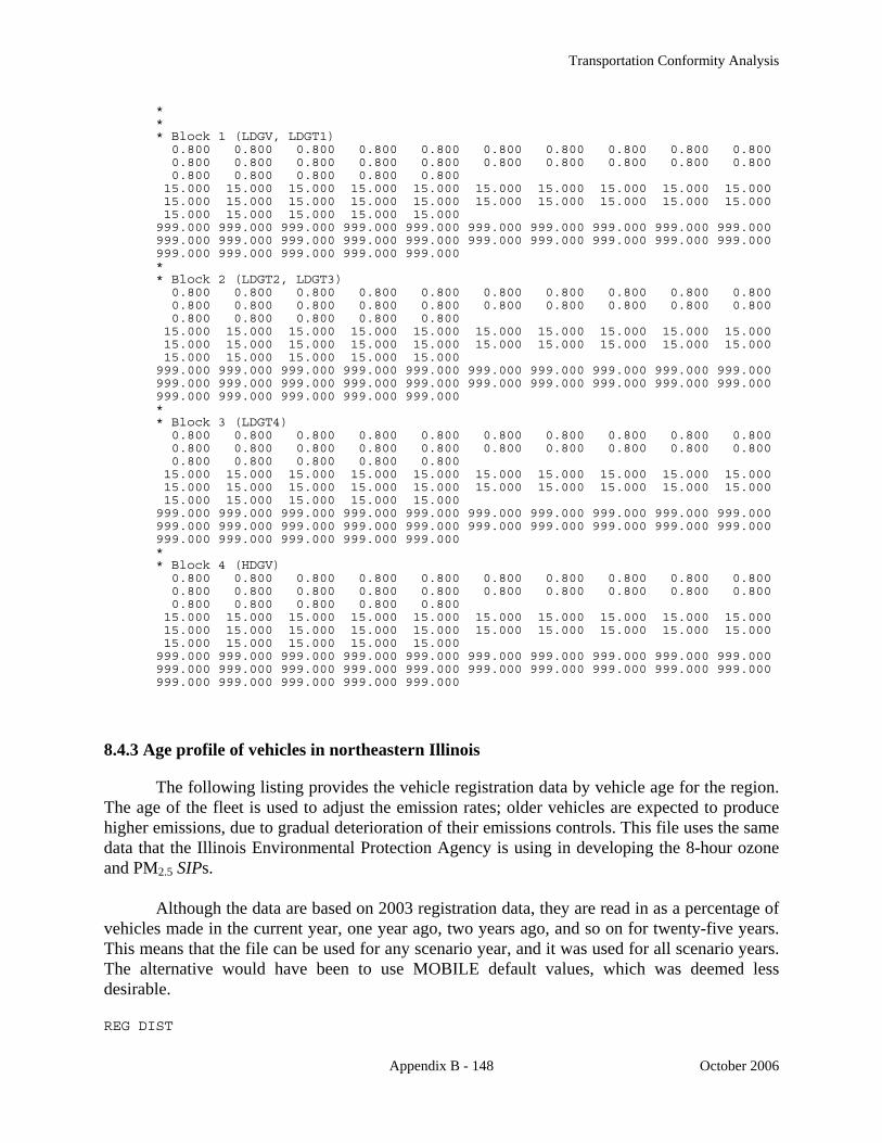
Transportation Conformity Analysis
Appendix B - 148 October 2006
* * * Block 1 (LDGV, LDGT1) 0.800 0.800 0.800 0.800 0.800 0.800 0.800 0.800 0.800 0.800 0.800 0.800 0.800 0.800 0.800 0.800 0.800 0.800 0.800 0.800 0.800 0.800 0.800 0.800 0.800 15.000 15.000 15.000 15.000 15.000 15.000 15.000 15.000 15.000 15.000 15.000 15.000 15.000 15.000 15.000 15.000 15.000 15.000 15.000 15.000 15.000 15.000 15.000 15.000 15.000 999.000 999.000 999.000 999.000 999.000 999.000 999.000 999.000 999.000 999.000 999.000 999.000 999.000 999.000 999.000 999.000 999.000 999.000 999.000 999.000 999.000 999.000 999.000 999.000 999.000 * * Block 2 (LDGT2, LDGT3) 0.800 0.800 0.800 0.800 0.800 0.800 0.800 0.800 0.800 0.800 0.800 0.800 0.800 0.800 0.800 0.800 0.800 0.800 0.800 0.800 0.800 0.800 0.800 0.800 0.800 15.000 15.000 15.000 15.000 15.000 15.000 15.000 15.000 15.000 15.000 15.000 15.000 15.000 15.000 15.000 15.000 15.000 15.000 15.000 15.000 15.000 15.000 15.000 15.000 15.000 999.000 999.000 999.000 999.000 999.000 999.000 999.000 999.000 999.000 999.000 999.000 999.000 999.000 999.000 999.000 999.000 999.000 999.000 999.000 999.000 999.000 999.000 999.000 999.000 999.000 * * Block 3 (LDGT4) 0.800 0.800 0.800 0.800 0.800 0.800 0.800 0.800 0.800 0.800 0.800 0.800 0.800 0.800 0.800 0.800 0.800 0.800 0.800 0.800 0.800 0.800 0.800 0.800 0.800 15.000 15.000 15.000 15.000 15.000 15.000 15.000 15.000 15.000 15.000 15.000 15.000 15.000 15.000 15.000 15.000 15.000 15.000 15.000 15.000 15.000 15.000 15.000 15.000 15.000 999.000 999.000 999.000 999.000 999.000 999.000 999.000 999.000 999.000 999.000 999.000 999.000 999.000 999.000 999.000 999.000 999.000 999.000 999.000 999.000 999.000 999.000 999.000 999.000 999.000 * * Block 4 (HDGV) 0.800 0.800 0.800 0.800 0.800 0.800 0.800 0.800 0.800 0.800 0.800 0.800 0.800 0.800 0.800 0.800 0.800 0.800 0.800 0.800 0.800 0.800 0.800 0.800 0.800 15.000 15.000 15.000 15.000 15.000 15.000 15.000 15.000 15.000 15.000 15.000 15.000 15.000 15.000 15.000 15.000 15.000 15.000 15.000 15.000 15.000 15.000 15.000 15.000 15.000 999.000 999.000 999.000 999.000 999.000 999.000 999.000 999.000 999.000 999.000 999.000 999.000 999.000 999.000 999.000 999.000 999.000 999.000 999.000 999.000 999.000 999.000 999.000 999.000 999.000
8.4.3 Age profile of vehicles in northeastern Illinois
The following listing provides the vehicle registration data by vehicle age for the region. The age of the fleet is used to adjust the emission rates; older vehicles are expected to produce higher emissions, due to gradual deterioration of their emissions controls. This file uses the same data that the Illinois Environmental Protection Agency is using in developing the 8-hour ozone and PM2.5 SIPs.
Although the data are based on 2003 registration data, they are read in as a percentage of
vehicles made in the current year, one year ago, two years ago, and so on for twenty-five years. This means that the file can be used for any scenario year, and it was used for all scenario years. The alternative would have been to use MOBILE default values, which was deemed less desirable.
REG DIST

Transportation Conformity Analysis
Appendix B - 149 October 2006
* * This file CHIRD03.D is derived from REGDATA.D, the default MOBILE6 * RD file. This file was created July 7, 2006 by Ross Patronsky * using registration data sent by Sam Long of IEPA on April 10, 2006. * * The file CHIRD01.D, used for conformity of the FY 2004 - 2009 TIP, * contains a lengthy explanation by Sam of his decision to use MOBILE6 * defaults for truck types. * * * M6 LDV from 4/10/06 S. Long email 1 0.0603 0.0804 0.0805 0.0818 0.0845 0.0773 0.0673 0.0670 0.0574 0.0620 0.0493 0.0449 0.0388 0.0331 0.0280 0.0233 0.0169 0.0122 0.0089 0.0067 0.0045 0.0025 0.0014 0.0009 0.0101 * * M6 LDT1 from 4/10/06 S. Long email 2 0.0796 0.1061 0.1062 0.0532 0.0365 0.0331 0.0358 0.0331 0.0546 0.0569 0.0676 0.0520 0.0396 0.0516 0.0443 0.0444 0.0300 0.0282 0.0188 0.0103 0.0052 0.0026 0.0021 0.0016 0.0066 * * M6 LDT2 from 4/10/06 S. Long email 3 0.0767 0.1023 0.1024 0.1053 0.1024 0.0893 0.0920 0.0766 0.0563 0.0517 0.0434 0.0348 0.0237 0.0157 0.0082 0.0061 0.0061 0.0015 0.0014 0.0010 0.0009 0.0005 0.0003 0.0002 0.0012 * * M6 LDT3 from 4/10/06 S. Long email 4 0.0674 0.0899 0.0900 0.0830 0.0867 0.1041 0.0614 0.0594 0.0433 0.0571 0.0479 0.0391 0.0303 0.0218 0.0232 0.0236 0.0185 0.0130 0.0092 0.0066 0.0049 0.0031 0.0017 0.0005 0.0143 * * M6 LDT4 from 4/10/06 S. Long email 5 0.0695 0.0926 0.0927 0.1167 0.1127 0.1290 0.0953 0.0753 0.0561 0.0505 0.0405 0.0135 0.0137 0.0049 0.0065 0.0041 0.0035 0.0024 0.0042 0.0029 0.0017 0.0010 0.0003 0.0002 0.0102 * * HDV2B (Heavy-duty vehicles 2B--M6 Default RDs) 6 0.0503 0.0916 0.0833 0.0758 0.0690 0.0627 0.0571 0.0519 0.0472 0.0430 0.0391 0.0356 0.0324 0.0294 0.0268 0.0244 0.0222 0.0202 0.0184 0.0167 0.0152 0.0138 0.0126 0.0114 0.0499 * HDV3 (Heavy-duty vehicles3, same RD as HDV2B, M6 Default RDs) 7 0.0503 0.0916 0.0833 0.0758 0.0690 0.0627 0.0571 0.0519 0.0472 0.0430 0.0391 0.0356 0.0324 0.0294 0.0268 0.0244 0.0222 0.0202 0.0184 0.0167 0.0152 0.0138 0.0126 0.0114 0.0499 * HDV4 (Heavy-duty vehicles 4, M6 default RDs) 8 0.0388 0.0726 0.0679 0.0635 0.0594 0.0556 0.0520 0.0486 0.0455 0.0425 0.0398 0.0372 0.0348 0.0326 0.0304 0.0285 0.0266 0.0249 0.0233 0.0218 0.0204 0.0191 0.0178 0.0167 0.0797 * HDV5 (Heavy-duty vehicles 5, same RD as HDV4, M6 Default) 9 0.0388 0.0726 0.0679 0.0635 0.0594 0.0556 0.0520 0.0486 0.0455 0.0425 0.0398 0.0372 0.0348 0.0326 0.0304 0.0285 0.0266 0.0249 0.0233 0.0218 0.0204 0.0191 0.0178 0.0167 0.0797 * HDV6 (Heavy-duty vehicless 6, same RD as HDV4, M6 Default) 10 0.0388 0.0726 0.0679 0.0635 0.0594 0.0556 0.0520 0.0486 0.0455 0.0425 0.0398 0.0372 0.0348 0.0326 0.0304 0.0285 0.0266 0.0249 0.0233 0.0218 0.0204 0.0191 0.0178 0.0167 0.0797 * HDV7 (Heavy-duty vehicles 7, same RD as HDV4, M6 Default) 11 0.0388 0.0726 0.0679 0.0635 0.0594 0.0556 0.0520 0.0486 0.0455 0.0425 0.0398 0.0372 0.0348 0.0326 0.0304 0.0285 0.0266 0.0249 0.0233 0.0218 0.0204 0.0191 0.0178 0.0167 0.0797 * HDV8A (Heavy-duty vehicles 8A same RD as HDV4, M6 Default) 12 0.0388 0.0726 0.0679 0.0635 0.0594 0.0556 0.0520 0.0486 0.0455 0.0425 0.0398 0.0372 0.0348 0.0326 0.0304 0.0285 0.0266 0.0249 0.0233 0.0218 0.0204 0.0191 0.0178 0.0167 0.0797 * HDV8B (Heavy-duty vehicles 8B,same RD as HDV4, M6 Default)

Transportation Conformity Analysis
Appendix B - 150 October 2006
13 0.0388 0.0726 0.0679 0.0635 0.0594 0.0556 0.0520 0.0486 0.0455 0.0425 0.0398 0.0372 0.0348 0.0326 0.0304 0.0285 0.0266 0.0249 0.0233 0.0218 0.0204 0.0191 0.0178 0.0167 0.0797 * HDBS (HDV School buses; this M6 RD default is assumed) 14 0.0393 0.0734 0.0686 0.0641 0.0599 0.0559 0.0522 0.0488 0.0456 0.0426 0.0398 0.0372 0.0347 0.0324 0.0303 0.0283 0.0264 0.0247 0.0231 0.0216 0.0201 0.0188 0.0176 0.0165 0.0781 * HDBT (HDV Transit buses; this M6 RD default is assumed) 15 0.0307 0.0614 0.0614 0.0614 0.0614 0.0614 0.0614 0.0614 0.0614 0.0613 0.0611 0.0607 0.0595 0.0568 0.0511 0.0406 0.0254 0.0121 0.0099 0.0081 0.0066 0.0054 0.0044 0.0037 0.0114 * Motorcycles (this M6 default RD is the same as M5a/b's default RD) 16 0.1440 0.1680 0.1350 0.1090 0.0880 0.0700 0.0560 0.0450 0.0360 0.0290 0.0230 0.0970 0.0000 0.0000 0.0000 0.0000 0.0000 0.0000 0.0000 0.0000 0.0000 0.0000 0.0000 0.0000 0.0000 *
8.4.4 Distribution of VMT by hour of the day in the region
The following listing shows the input for distributing VMT over the day. MOBILE uses this information to adjust emission rates, since rates are generally higher in warmer parts of the day.
The travel model’s use fixed factors to apportion vehicle trip tables by time-of-day. At
present, these factors do not vary by scenario year. VMT BY HOUR * * Fraction of all vehicle miles traveled by hour of the day. * First hour is 6 a.m. * These values developed from conf2000 scenario 2207 (mf13.xls) for M6 test w/ M5b params * 0.0443 0.0803 0.0803 0.0577 0.0576 0.0576 0.0576 0.0576 0.0680 0.0680 0.0793 0.0793 0.0511 0.0511 0.0110 0.0110 0.0110 0.0110 0.0110 0.0110 0.0110 0.0110 0.0110 0.0110
8.4.5 5. Dummy files assigning all VMT to local streets or freeway ramps
The following listing shows the input file used to assign all VMT to local streets. This is used in one of the MOBILE6 “runs” to generate emission rates for these facilities. A similar file (not shown) assigns all VMT to local streets. For brevity’s sake, the file is truncated after the first vehicle type. For arterials and freeways, the AVERAGE SPEED command performs the function of assigning all VMT to one facility type.
VMT BY FACILITY * * This is [D:\]AREASPEC\FVMTLCL.DEF, based on FVMT.DEF, the * "default" FVMT file supplied with the M6 model. * * VMT fractions are listed for 28 vehicle classes for each hour of * the day starting at 6AM. There are 24 sets of four values for * each vehicle type. The VMT fractions by hour are the same * for all vehicle classes. * * The four values in each line represent the VMT distribution on

Transportation Conformity Analysis
Appendix B - 151 October 2006
* freeway, arterial, local and ramps--in that order--as shown. * * See M6UG 2.8.5.1.f., p. 49, or CLASLIST.TXT for further info. * (The CLASLIST file describes the vehicle classes.) * This file is modified to give 100% LOCAL * * Veh Int& Arts& Local *Class Fwys Colls Rd/St Ramps *----- ---- ----- ----- ----- * 1 0.000 0.000 1.000 0.000 0.000 0.000 1.000 0.000 0.000 0.000 1.000 0.000 0.000 0.000 1.000 0.000 0.000 0.000 1.000 0.000 0.000 0.000 1.000 0.000 0.000 0.000 1.000 0.000 0.000 0.000 1.000 0.000 0.000 0.000 1.000 0.000 0.000 0.000 1.000 0.000 0.000 0.000 1.000 0.000 0.000 0.000 1.000 0.000 0.000 0.000 1.000 0.000 0.000 0.000 1.000 0.000 0.000 0.000 1.000 0.000 0.000 0.000 1.000 0.000 0.000 0.000 1.000 0.000 0.000 0.000 1.000 0.000 0.000 0.000 1.000 0.000 0.000 0.000 1.000 0.000 0.000 0.000 1.000 0.000 0.000 0.000 1.000 0.000 0.000 0.000 1.000 0.000 0.000 0.000 1.000 0.000 2 0.000 0.000 1.000 0.000 0.000 0.000 1.000 0.000
Note that there are additional lines in the definition file for each of the twenty-eight
vehicle types; each vehicle type having one line for each hour of the day.
8.4.6 Changes to MOBILE6 input for analysis years 2007, 2010, 2020 and 2030
A review of the preceding listings shows that the year record in each scenario is different, so this record is changed in each batch file.
As discussed previously, the inspection & maintenance and vehicle age profile data are
not known to be different for different scenario years, so the same local data were used for all scenario years. The distribution of VMT by hour of the day does not vary from year to year, owing to the way in which the travel assignment model is run. As a result, the same data were used for all scenario years.


CATS WORK PROGRAM COMMITTEE THOMAS B. RICKERT, Chairman Assistant Director Kane County Division of Transportation JACK GRONER, Vice Chairman Department Head Commuter Rail Division of the RTA – Metra DICK SMITH Director, Office of Planning & Programming Illinois Department of Transportation CLARITA LAO Engineer of Program Development District 1, Illinois Department of Transportation JASON TAI Director Division of Public and Intermodal Transportation Illinois Department of Transportation MICHAEL D. ROGERS Environmental Protection Specialist Illinois Environmental Protection Agency JOHN DeLAURENTIIS Deputy Executive Director Regional Transportation Authority RONALD THOMAS Executive Director Northeastern Illinois Planning Commission ARLENE MULDER Mayor, Village of Arlington Heights Representing CATS Council of Mayors LUANN HAMILTON Deputy Commissioner for Project Development Chicago Department of Transportation JEFFREY SRIVER General Manager, Strategic Planning Chicago Transit Authority BENET HALLER Director, Urban Design and Planning Chicago Department of Planning & Development RODNEY BETTENHAUSEN Advance Planning Engineer Cook County Highway Department CHUCK TOKARSKI County Engineer DuPage County Division of Transportation
AL GIERTYCH Assistant County Engineer Lake County JASON OSBORN Transportation, Planning and Program Coordinator McHenry County BRUCE GOULD Assistant County Engineer Will County FRAN KLAAS County Engineer Kendall County ROCKY DONAHUE Director of Government Affairs Suburban Bus Board – Pace THOMAS A. ZAPLER Special Representative, Union Pacific Railroad Representing Class 1 Railroads JOHN D. RITA South Suburban Mass Transit District Representing Mass Transit Districts PAUL M. LOSOS Sunrise Transportation, Inc. Representing Private Transportation Providers MARY WELLS Sr. Manager. of Strategic Planning & Programming Illinois State Toll Highway Authority CHRISTOPHER DiPALMA Metropolitan Planning Engineer Federal Highway Administration VANESSA ADAMS Community Planner Federal Transit Administration STEVEN STRAINS Director of Transportation Development Northwestern Indiana Regional Planning Commission DONALD P. KOPEC Executive Director Chicago Area Transportation Study Patricia Berry, Secretary Acting Deputy for Programming Chicago Area Transportation Study


![· Web viewList of Tables. List of Abbreviated Terms. Appendix C [appendix title] [Project Title] Air Quality Conformity Analysis12 [Project Title] Air Quality Conformity Analysis13](https://img.dokumen.tips/doc/110x75/5aad7a067f8b9aa9488e517a/viewlist-of-tables-list-of-abbreviated-terms-appendix-c-appendix-title-project.jpg)