Transportation Behavioral Modelling: An Introduction

Arnab Jana, PhD

Associate Professor

Centre for Urban Science & Engineering

Indian Institute of Technology Bombay

September 17, 2021

The 20th Behavior Modeling Summer SchoolSep. 15 – 19 , 2021 @ The University of Tokyo

About the Urban Infrastructure Research group, CUSE IIT Bombay• Infrastructure and behavioral modelling

• Application of AI in urban planning

• Livability and quality of life

2

Why are we interested in Travel Demand Modelling?

Forecast - Transportation Demand

PeopleTransportation system

Changes in the Attributes

UserVehicle/ CarrierRoadway/ FacilityEnvironment

3

Contents

• Introduction to four step model

• Choice Models

• Activity Based Modelling Approach

4

Introduction

• Demand for Travel is a derived Demand

• Components of Transportation System1. User

2. Vehicle/ Carrier

3. Roadway/ Facility

4. Environment

• Transportation systems problems1. Congestion

2. Pollution

3. Safety

4. Parking

5

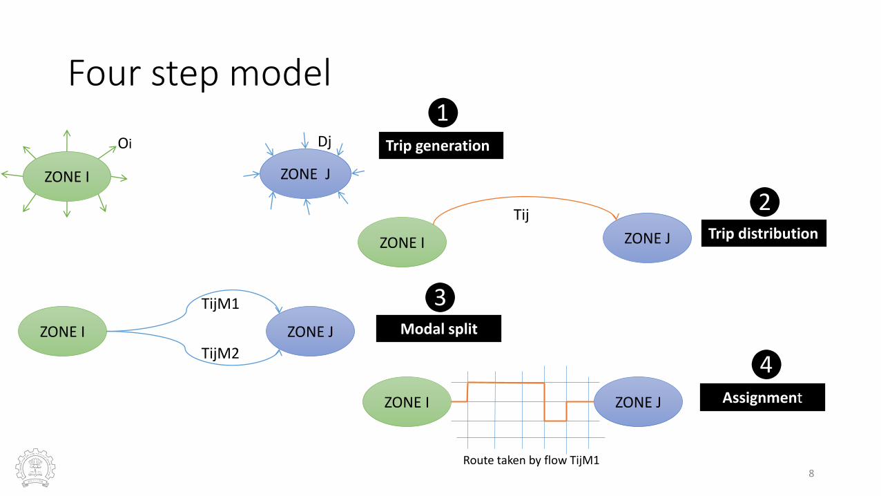
Four step model

6

Four step modelIn

pu

ts Transportation system Characteristics

Land use – activity system characteristics

Urb

an T

ran

spo

rtat

ion

mo

del

sy

stem ❶Trip Generation

(How many trips)

❷Trip Distribution (Where do they go?)

❸Mode Choice (By what mode?)

❹Traffic Assignment (By what route?)

Ou

tpu

ts Traffic flow on network

Quantity (Volume)

Quality (Speed)

7

Four step model

ZONE I ZONE J

ZONE I ZONE J

ZONE I ZONE J

ZONE I ZONE J

Oi Dj

Tij

TijM1

TijM2

Trip generation

Trip distribution

Modal split

Assignment

Route taken by flow TijM1

❶

❷

❸

❹

8

ExampleTijmrsp

Production

1 47

2 663 110

Pi

Work

2

6

Edud.

1Other

9

Trip Purpose

Education

Work

Other

3

12

2

17

Tijmrp

2 3

18 19

32 4

To Zones

1

1 10

2 30

3 5 40 65

45 90 88

47

66

110

223

From

Zones

Attraction

1 45

2 903 88

Aj

ZONE 1Pi: 47; Aj: 45

ZONE 2Pi: 66; Aj: 90

ZONE 3Pi: 110; Aj: 88

Tijm

Mode II

25

15

Mode I

40 Route C 3

Route B 17

Route A 5

Tijmr

Tijmrs(Income)

Medium

3

5

High

9Low

17

9

❶Trip Generation

• Aims at predicting the total number of trips generated by (Oi) and attracted to (Dj) each zone of the study area

• Trip or Journey: This is a one-way movement from a point of origin to a point of destination

• Home-based (HB) Trip This is one where the home of the trip maker is either the origin or the destination of the journey

• Non-home-based (NHB) Trip This, conversely, is one where neither end of the trip is the home of the traveler

10

Classification of Trips

• travel to work

• travel to school or college (education trips)

• shopping trips

• social and recreational journeys

• escort trips (to accompany or collect somebody else)

• other journeys

11

❷Trip Distribution

• The purpose of the trip distribution is to estimate ‘zone to zone’ movements, i.e., trip interchanges

Gravity Model

Probability that a trip of a particular purpose k produced at zone i will be attracted to zone j, is proportional to the attractiveness or ‘pull’ of zone j, which depends on two factors.

One factor is the magnitude of activities related to the trip purpose k in zone j, and the other is the spatial separation of the zones i and j.

12

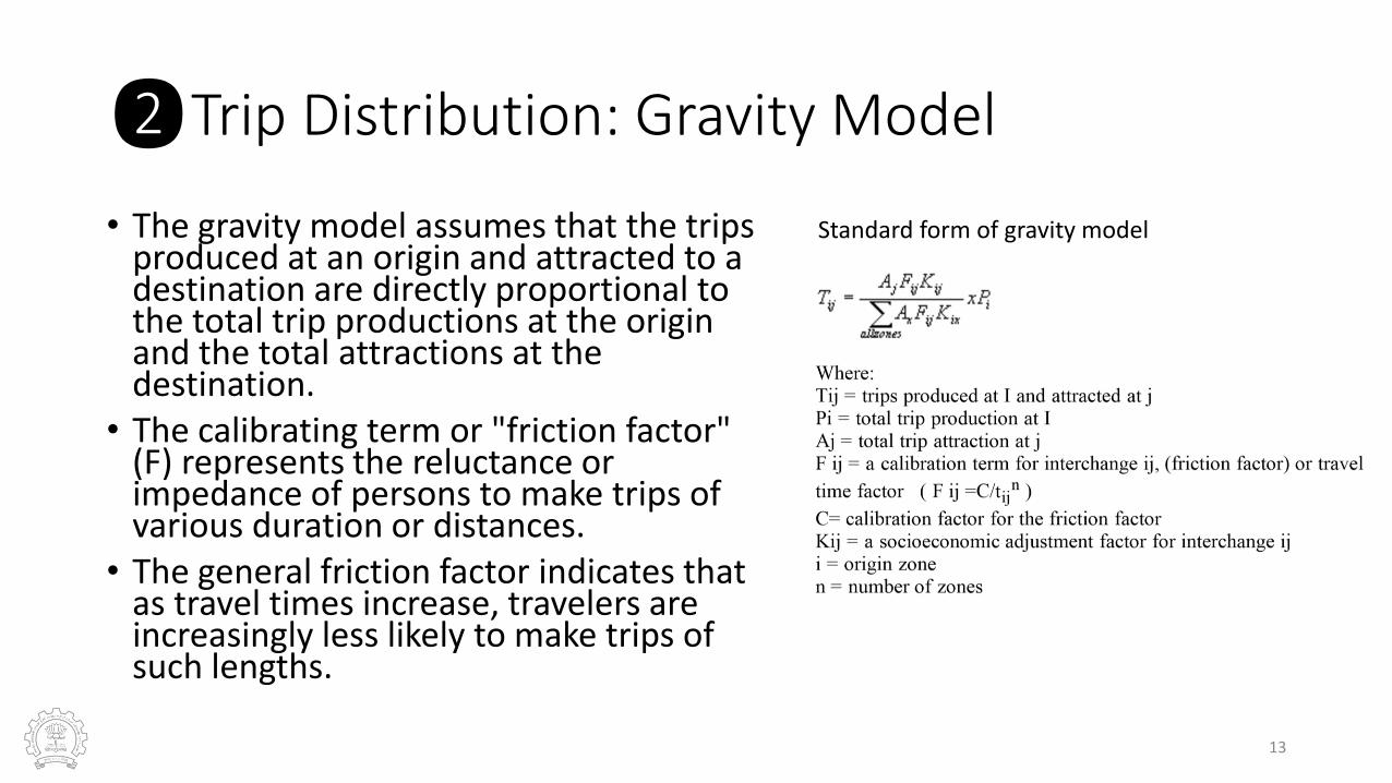
❷Trip Distribution: Gravity Model

• The gravity model assumes that the trips produced at an origin and attracted to a destination are directly proportional to the total trip productions at the origin and the total attractions at the destination.

• The calibrating term or "friction factor" (F) represents the reluctance or impedance of persons to make trips of various duration or distances.

• The general friction factor indicates that as travel times increase, travelers are increasingly less likely to make trips of such lengths.

13

Standard form of gravity model

❸Mode Choice

• Relates the probability of transit usage to explanatory variables in mathematical form

• Factors Affecting Mode Choice

Factors that may explain a trip maker’s choosing a specific mode of transportation for a trip are grouped commonly as follows:

• Trip Makers Characteristics: • Income • Car-Ownership • Car Availability • Age

• Trip Characteristics: • Trip Purpose - work, shop, recreation, etc. • Destination Orientation - CBD vs. non-CBD • Trip Length

• Transportation Systems Characteristics • Waiting time • Speed • Cost • Comfort and Convenience • Access to terminal or transfer location

14

15

Bus - 40 minutes

Car - 35 minutes

I chose CAR

Actual Behavior – Reveled Preference (RP) Data

❸Mode Choice

16

Bus - 40 minutes

Car - 35 minutes

If new service is introduced, I

will chose Metro

Hypothetical Behavior – Stated Preference (SP) Data

A new service introducedMetro - 15 minutes

❸Mode Choice

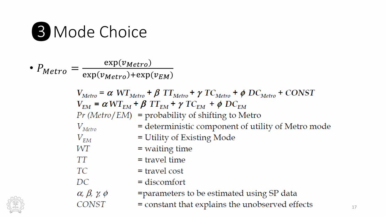
• 𝑃𝑀𝑒𝑡𝑟𝑜 =exp(𝑣𝑀𝑒𝑡𝑟𝑜)

exp 𝑣𝑀𝑒𝑡𝑟𝑜 +exp(𝑣𝐸𝑀)

17

❸Mode Choice

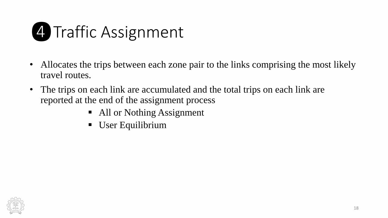
❹Traffic Assignment

• Allocates the trips between each zone pair to the links comprising the most likely travel routes.

• The trips on each link are accumulated and the total trips on each link are reported at the end of the assignment process

All or Nothing Assignment

User Equilibrium

18

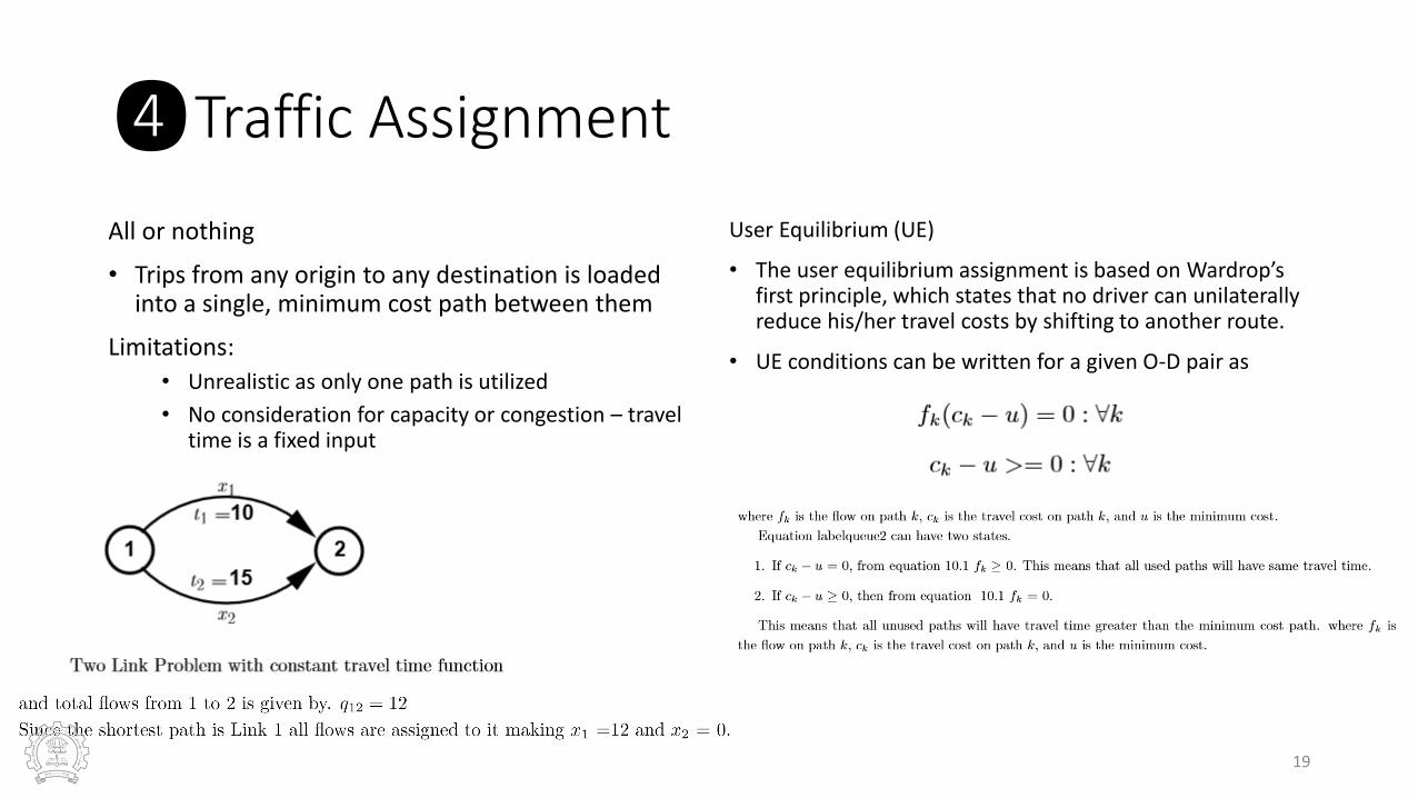
❹Traffic Assignment

All or nothing

• Trips from any origin to any destination is loaded into a single, minimum cost path between them

Limitations:

• Unrealistic as only one path is utilized

• No consideration for capacity or congestion – travel time is a fixed input

User Equilibrium (UE)

• The user equilibrium assignment is based on Wardrop’sfirst principle, which states that no driver can unilaterally reduce his/her travel costs by shifting to another route.

• UE conditions can be written for a given O-D pair as

19

Choice models

20

Choice Models

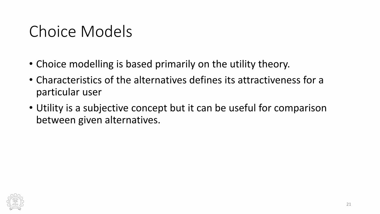
• Choice modelling is based primarily on the utility theory.

• Characteristics of the alternatives defines its attractiveness for a particular user

• Utility is a subjective concept but it can be useful for comparison between given alternatives.

21

Utility Theory

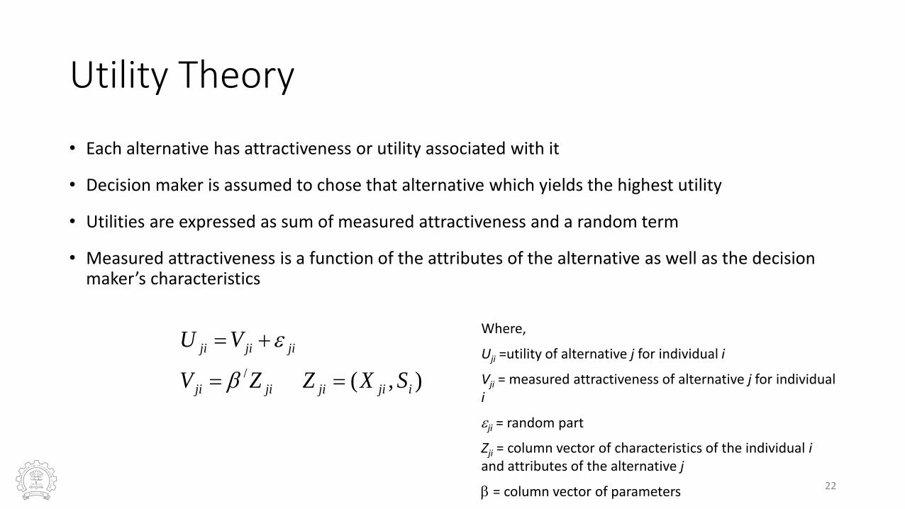
• Each alternative has attractiveness or utility associated with it

• Decision maker is assumed to chose that alternative which yields the highest utility

• Utilities are expressed as sum of measured attractiveness and a random term

• Measured attractiveness is a function of the attributes of the alternative as well as the decision maker’s characteristics

),(/

ijijijiji

jijiji

SXZZV

VU

Where,

Uji =utility of alternative j for individual i

Vji = measured attractiveness of alternative j for individual i

ji = random part

Zji = column vector of characteristics of the individual iand attributes of the alternative j

= column vector of parameters 22

Utility Theory

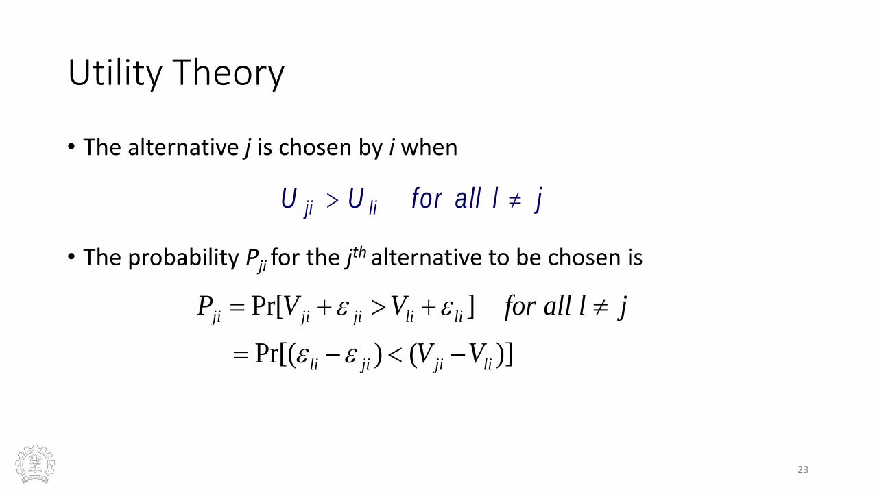
• The alternative j is chosen by i when

• The probability Pji for the jth alternative to be chosen is

jla llforUU liji

)]()Pr[(

]Pr[

lijijili

lilijijiji

VV

jlallforVVP

23

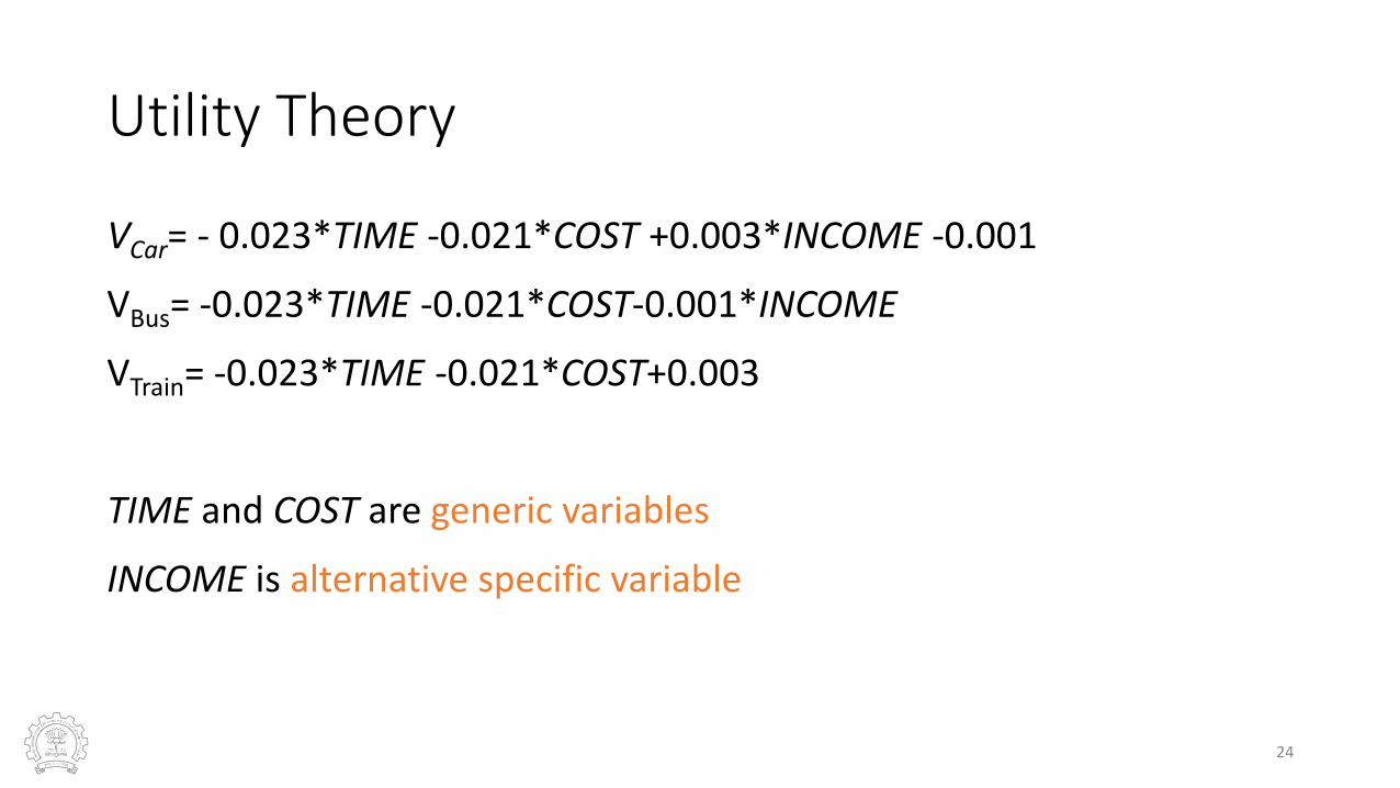
Utility Theory

VCar= - 0.023*TIME -0.021*COST +0.003*INCOME -0.001

VBus= -0.023*TIME -0.021*COST-0.001*INCOME

VTrain= -0.023*TIME -0.021*COST+0.003

TIME and COST are generic variables

INCOME is alternative specific variable

24

Variables …

• Generic Variable - Variable that appears in the utility functions of all alternatives in a generic sense and has same coefficient estimate for all the alternatives

• Alternative Specific Variable - Variable that appears only in the utility function of those alternatives to which it is specific and has different coefficient estimate for each of the alternatives

• Alternative Specific Constant - Takes care of unexplained effects

25

Some Limitations of 4-step TDM

• Traditional travel demand models ignore travel as a demand derived from activity participation decisions

• Does not incorporate the reason for traveling – the activity at the end of the trip

• Trips treated as independent and ignores their spatial, temporal, and social interactions

• Heavy emphasis on commuting trips and Home-based trips

• Limited policy sensitivity (TAZs are hard to use in policy analysis)

26

Activity Based Modelling

27

Necessity of Activity Based Travel Demand Modelling• Development of ABM due to poor forecasting results achieved in the

trip based aggregate demand models

• Introduce - road pricing

• new technologies - ( Internet and mobile phones)

• For solving urbanization problems, understanding behaviouralchanges of people in developing countries is necessary

28

Activity Based Modelling – Historical

• ABM belongs to the 3rd generation of travel demand models

• Trip based 4-step models

• Disaggregate trip based models (1980’s & 1990’s)

• Activity based models

• In ABM the basic unit of analysis is the activities of individuals/households

• Activity Based Models (ABM) predict travel behavior as a derivative of activities (i.e., derived demand)

• Travel decisions are part of a broader process based on modeling the demand for activities rather than merely modeling trips

• ABM are based on the theories of Hägerstrand (1970) and Chapin (1974)

• Hägerstrand focused on personal and social constraints

• Chapin focused on opportunities and choices

• Theory is that activity demand is motivated by basic human desires for: survival, ego gratification, and social encounters

29

ABM Approach

• Travel demand is derived from activities that individuals need/wish toperform

• Sequence/patterns of behavior, not individual trips, are the unit of analysis

• Household and other social structures influence travel and activitybehavior

• Spatial, temporal, transportation, and interpersonal interdependenciesconstrain activity/travel behavior

• Activity based approaches aim at predicting which activities are conductedwhere, when, for how long, with whom, by mode, and ideally also theimplied route decision

30

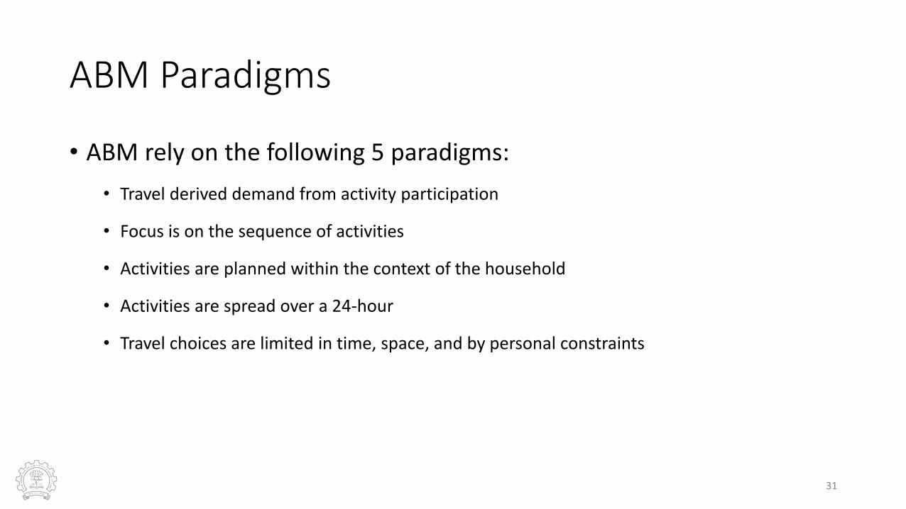
ABM Paradigms

• ABM rely on the following 5 paradigms:

• Travel derived demand from activity participation

• Focus is on the sequence of activities

• Activities are planned within the context of the household

• Activities are spread over a 24-hour

• Travel choices are limited in time, space, and by personal constraints

31

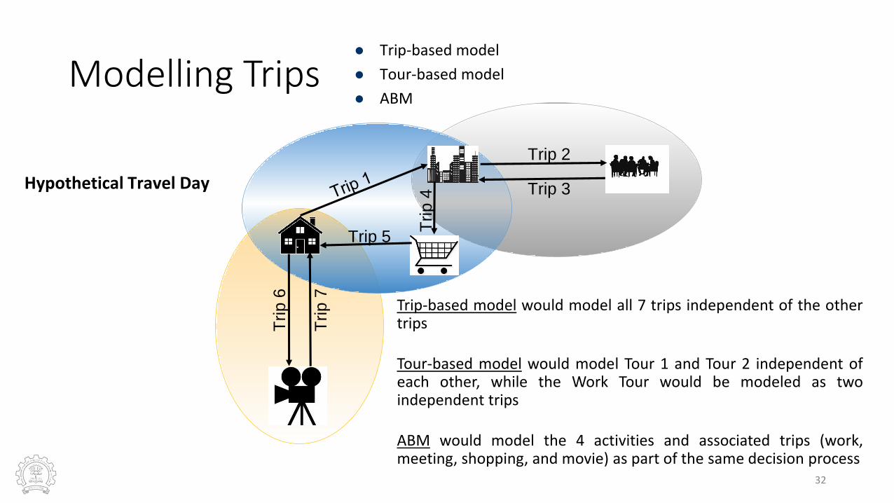
Modelling Trips

Trip 5

Trip 4

Trip 3

Trip 2

Trip 6

Trip 7

Hypothetical Travel Day

Trip-based model

Tour-based model

ABM

Trip-based model would model all 7 trips independent of the othertrips

Tour-based model would model Tour 1 and Tour 2 independent ofeach other, while the Work Tour would be modeled as twoindependent trips

ABM would model the 4 activities and associated trips (work,meeting, shopping, and movie) as part of the same decision process

32

Activities in Time and Space

Tim

eH

W

L

S

Activities:H … Home W … Work L … Leisure S … Shopping 33

Activities in Time and SpaceTi

me

Space

H

W

WF

FL

LS

H

H

W

F

L

S

Home

Work- Mandatory

Social connection- Leisure

Cinema- Leisure

Shopping- MaintenanceTravel- Mandatory

Travel- Leisure

Travel- Maintenance

Activity time- Mandatory

Activity time- Leisure

Activity time- Maintenance

Source: Varun Varghese

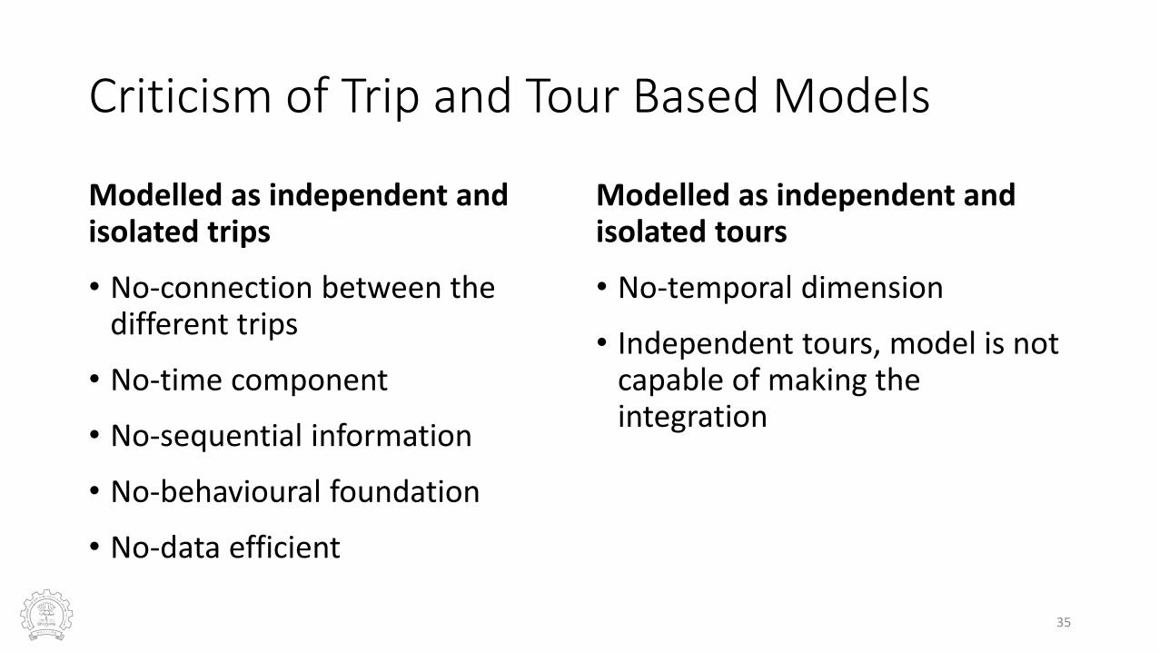
Criticism of Trip and Tour Based Models

Modelled as independent and isolated trips

• No-connection between the different trips

• No-time component

• No-sequential information

• No-behavioural foundation

• No-data efficient

Modelled as independent and isolated tours

• No-temporal dimension

• Independent tours, model is not capable of making the integration

35

Advantages of ABM

• Theoretically based on human behavior

• Better understanding and prediction of traveler behavior

• Based on decision-making choices present in the “real-world”

• Use of disaggregate data

• Inclusion of time-of-day travel choices

36

Activity Patterns (Schedule)

A sequence of activities, or a schedule, defines a path in space and time

What defines a person’s activity pattern?• Total amount of time outside home

• Number of trips per day and their type

• Allocation of trips to tours

• Allocation of tours to particular HH members

• Departure time from home

• Arrival time at home in the evening

• Activity duration

• Activity location

• Mode of transportation

• Travel party

37

A Person’s Daily Travel Pattern (conventional model)

Home

Work

Shop

Diner

TRIPS:-2 HBW-1 HBS-1 HBO-1 NHB

38

A Person’s Daily Travel Pattern (activity based model)

Home

Work

Shop

Dinner

TRIPS:-2 HBW-1 HBS-1 HBO-1 NHB

-2 Home based tours (chains)-Timing of all trips-Duration of activity at each location

5:30 PM

7:00 PM

7:30 PM9:30 PM

9:00 PM7:30 AM

8:15 PM

4:30 PM

5:15 PM

39

All Household Members’ Travel Pattern (activity based model)

Home

School

Shop

Home to School by Car

Diner

7:00 PM

9:30 PM

9:00 AM

5:15 PM

Work to School by CarSchool to Home by Car

WorkSchool to Work by Car

2:30 PM

8:00 AM

3:30 PM

Home

Work

Shop

Home to Work by BusDiner

Shop to Diner by car5:30 PM

7:30 PM

9:30 PM

9:00 PM

7:30 AM

8:15 PM

4:30 PM

5:15 PM

Work to Home by Bus

40

Some Key Aspects of Activity Based Models

• Trips are linked for each person in a day

• Timing and durations are included

• Entire daily travel patterns are linked

• Car use is associated to needs (take child to school, drive together toshop & dine and back )

41

Survey Instrument

• Household Information

• Person Information

• Activity Information

Activity Diary

Activities classified:• Work related activities

• Maintenance activities

• Leisure activities

42

Modelling approaches

• Econometric modelling

• Rule based modelling

• Markov models

• Microsimulation modelling

43

CONCLUSION

• Conventional four stage-planning models for travel demandforecasting includes the lack of behavioral foundation, overdependence on trips, and insensitivity to policy changes.

• There is a need to develop the models which will take into accountabove criteria's to improve the travel demand.

• The new modeling approach i.e. activity based travel demandmodeling has good scope in developing countries due to its morefocus on behavioral aspect of people.

44

Best wishes !!

45