Embed Size (px)
DESCRIPTION
Transmission_stability_enhancement_using_wide_area_measurement_systems_WAMS_and_critical_clusters
Citation preview
Transmission Stability Enhancement using Wide Area Measurement Systems (WAMS) and Critical Clusters
Hamza A. Alsafih
A thesis submitted for the degree of Doctor of Philosophy (PhD)
University of Bath
Department of Electronic and Electrical Engineering
February 2013
COPYRIGHT
Attention is drawn to the fact that copyright of this thesis rests with its author. This copy
of the thesis has been supplied on condition that anyone who consults it is understood to
recognise that its copyright rests with the author and they must not copy it or use
material from it except as permitted by law or with the consent of the author.
This thesis may be made available for consultation within the University Library and
may be photocopied or lent to other libraries for the purpose of consultation.

Abstract
i
Abstract
Due to the on-going worldwide trend towards investment in de-regulated electricity
markets driven by political, economic and environmental issues, increasing
interconnection between modern power systems has made power system dynamic
studies much more complex. The continuous load growth without a corresponding
increase in transmission network capacities has stressed power systems further and
forced them to operate closer to their stability limits. Large power transfers between
utilities across the interconnections stress these interconnections. As a result, stability of
such power systems becomes a serious issue as operational security and reliability
standards can be violated. On the other hand, the evolving technology of Wide-Area
Measurement Systems (WAMS) has led to advanced applications in Wide-Area
Monitoring, Protection and Control (WAMPAC) systems [1], which offer a cost-
effective solutions to tackle these challenging issues.
The main focus of this research project was to develop a wide-area based stability
enhancement control scheme for large interconnected power systems. A new method to
identify coherent clusters of synchronous generators involved in wide area system
oscillations was the initial part of the work. The coherent clusters identification method
was developed to utilise measurements of generators speed deviation signals combined
with measurements of generators active power outputs to extract coherency property
between system’s generators. The obtained coherency property was then used by an
agglomerative clustering algorithm to group system’s generators into coherent clusters.
The identification of coherent clusters was then taken as a base to propose a new
structure of a WAMS based stability control scheme. The concept of WAMS and a
nonlinear control design approach (fuzzy logic theory) was used to provide a
comprehensive new control algorithm. The objectives of the developed control scheme
were to enhance and improve the control performance of modern power systems. Thus,
allowing improved dynamic performance under severe operation conditions. These
objectives were achieved by means of enhanced damping of power system oscillations,
enhanced system stability and improved transfer capabilities of the power system
allowing the stability limit to be approached without threatening the system security and
reliability.

Acknowledgment
ii
Acknowledgment
I would like to express my sincere gratitude to all those without whom this research and
its outcome would not have been accomplished.
First, I would like to thank the University of Bath and, in particular, the Department of
Electronic and Electrical Engineering for providing the fine facilities and sufficient
subsistence support to help me concentrate solely on the project. I would also like to
thank the SuperGen FlexNet UK Consortium and the Libyan Cultural Affairs for the
financial support of my PhD.
Second, I would like to express my sincere gratitude and deepest appreciation to Dr.
Rod Dunn for presenting the opportunity to undertake this research project and also for
his support, supervision and invaluable guidance through the course of the work.
Furthermore, I would also like to thank graduate students and staff in the Centre of
Sustainable Power Distribution at the University of Bath for creating an atmosphere of
friendship, mutual understanding and cooperation.
Last but not least, I am grateful for my family for their infinite support and
encouragement through all my study and life. My great gratefulness and sincere thanks
go to my parents, my brothers and my sisters for their love and kindness. A special
thanks to my wife for her support along the way.
Thank you very much to all of you!
Hamza A. Alsafih
Bath, February 2013

Contents
iii
Contents
Abstract .............................................................................................................................. i
Acknowledgment .............................................................................................................. ii
Contents ........................................................................................................................... iii
List of Figures .................................................................................................................. vi
List of Tables..................................................................................................................... x
List of Abbreviations........................................................................................................ xi
List of Symbols .............................................................................................................. xiii
Chapter 1: Introduction ..................................................................................................... 1
1.1. Today’s Challenges for Power Systems Operation and Control ............................ 1
1.2. Responses to the Challenges .................................................................................. 2
1.3. Thesis Overview..................................................................................................... 4
1.4. Research Objectives ............................................................................................... 5
1.5. Thesis Structure and Content ................................................................................. 6
1.6. Contribution from this Research ............................................................................ 9
Chapter 2: Wide-area Measurement Systems WAMS .................................................... 11
2.1. Overview .............................................................................................................. 11
2.2. WAMS Applications in Power Systems .............................................................. 14
2.2.1. Protection ...................................................................................................... 15
2.2.2. Control .......................................................................................................... 16
2.2.3. Monitoring and Recording ............................................................................ 18
2.3. Summary .............................................................................................................. 19
Chapter 3: Power System Oscillations and Control Measures........................................ 20
3.1. Overview .............................................................................................................. 20
3.2. Wide-Area based Control Schemes for Power System Oscillations Damping .... 21
3.2.1. Decentralised Control Strategies ................................................................... 22
3.2.2. Centralised Control Strategies....................................................................... 25
3.2.3. Multi-agent Control Strategies ...................................................................... 28
3.3. Power System Oscillations and the Concept of Coherent Clusters...................... 30
3.4. Identification of Coherent Clusters in Power Systems ........................................ 32
3.5. Summary .............................................................................................................. 34
Chapter 4: A Novel WAM based Technique to Identify Coherent Clusters in Multi-
machine Power Systems .................................................................................................. 35

Contents
iv
4.1. Overview .............................................................................................................. 35
4.2. Methodology ........................................................................................................ 36
4.2.1. Coherency Identification ............................................................................... 37
4.2.2. The Events’ Effect on the Clustering ............................................................ 38
4.3. Algorithm Implementation (Software and Simulation) ....................................... 41
4.4. Test Systems ........................................................................................................ 42
4.4.1. Case Study 1: 16 generator 68 bus test system ............................................. 43
4.4.2. Verification of clusters formation ................................................................. 51
4.4.3. Case Study 2: IEEE 10 generators 39 bus system......................................... 53
4.5. Summary .............................................................................................................. 60
Chapter 5: Identification of Key Clusters for Potential WAM based Control ................ 62
5.1. Overview .............................................................................................................. 62
5.2. Concept and Implementation ............................................................................... 63
5.3. Case Study ............................................................................................................ 64
5.4. Summary .............................................................................................................. 77
Chapter 6: Development of a Novel WAM based Control Scheme for Stability
Enhancement ................................................................................................................... 78
6.1. Overview .............................................................................................................. 78
6.2. Excitation Control and Stabilisation (advantages and limitations) ...................... 79
6.3. Fuzzy Logic and its Application to Power Systems ............................................ 83
6.3.1. Application of Fuzzy Logic in Power Systems ............................................. 85
6.3.2. Fuzzy Logic based Power System Stabilisers FPSS ..................................... 88
6.4. A Novel Design Structure for Wide-area based Fuzzy Logic PSS .................... 106
6.4.1. Structure of the Proposed Controller........................................................... 107
6.5. Summary ............................................................................................................ 121
Chapter 7: Implementation of the Designed Controller in Multi-area Power Systems 123
7.1. Case Study 1: 16-Generator 5-Area Test System .............................................. 125
7.2. Case Study 2: IEEE 39 Bus 2-Area Test System ............................................... 153
7.3. Summary ............................................................................................................ 170
Chapter 8: Conclusions and Future Work ..................................................................... 171
8.1. Conclusions and Limitations .............................................................................. 171
8.2. Future Work ....................................................................................................... 174
References ..................................................................................................................... 177
Appendices .................................................................................................................... 185

Contents
v
Appendix A1: Data of the 16 generator 68 bus New England / New York test system
................................................................................................................................... 185
Appendix A2: Data of the 10 machines-39-bus IEEE test system............................ 190
Appendix A3: Data of the two-area four machine test system ................................. 192
Appendix A4: Related Publications .......................................................................... 193

List of Figures
vi
List of Figures
Figure 2-1: Elements of Phasor Measurement Unit PMU ............................................. 12
Figure 2-2: A simplified WAMS architecture ............................................................... 13
Figure 3-1: Framework of centralised and decentralised control schemes .................... 22
Figure 3-2: Two-level PSS design architecture ............................................................. 24
Figure 3-3: General architecture of a decentralised / hierarchical PSS design .............. 25
Figure 3-4: The hierarchical controller structure ........................................................... 26
Figure 3-5: General structure of a wide-area centralised damping control system ........ 27
Figure 3-6: Framework of multi-agent based controllers ............................................... 29
Figure 3-7: Components of SPSS .................................................................................. 30
Figure 3-8: Conceptual input/output scheme of SPSS ................................................... 30
Figure 4-1: Typical response of generators group (rotors speed deviation) to a system
disturbance ...................................................................................................................... 36
Figure 4-2: Active power outputs of generators group during a system disturbance ..... 39
Figure 4-3: Flowchart for the proposed clustering algorithm ......................................... 41
Figure 4-4: The 16 generator 68 bus test system ............................................................ 44
Figure 4-5: Case Study 1- The cluster tree...................................................................... 47
Figure 4-6: Case Study 1- The dissimilarity coefficient at each clustering step ............. 47
Figure 4-7: The five clusters for the 16 generator 68 bus test system ............................ 50
Figure 4-8: The equivalent speed deviation signals for the five clusters' system ........... 52
Figure 4-9: The equivalent speed deviation signals for clusters 1 & 2 along with their
representative weighted response .................................................................................... 52
Figure 4-10: IEEE 10 machines 39 bus system .............................................................. 54
Figure 4-11: Case Study 2- The cluster tree.................................................................... 56
Figure 4-12: Case Study 2- The dissimilarity coefficient at each clustering step ........... 56
Figure 4-13: The two clusters of the IEEE 39 bus system .............................................. 59
Figure 5-1: The five clusters of the 16 generator 68 bus test system with critical tie-lines
......................................................................................................................................... 65
Figure 5-2: Fault on line 1-2/ 16 machine test system .................................................... 68
Figure 5-3: Fault on line 1-47/ 16 machine test system .................................................. 69
Figure 5-4: Fault on line 1-27/ 16 machine test system .................................................. 70
Figure 5-5: Fault on line 8-9/ 16 machine test system .................................................... 71
Figure 5-6: Fault on line 46-49/ 16 machine test system ................................................ 72

List of Figures
vii
Figure 5-7: Fault on line 50-51/ 16 machine test system ................................................ 73
Figure 5-8: Fault on line 41-42/ 16 machine test system ................................................ 75
Figure 5-9: Fault on line 42-52/ 16 machine test system ................................................ 76
Figure 6-1: Typical generating unit with most auxiliary components ........................... 80
Figure 6-2: Block diagram of conventional PSS ........................................................... 82
Figure 6-3: Basic configuration of Fuzzy Logic Controllers (FLC) .............................. 89
Figure 6-4: Triangular membership functions for FPSS input and output variables ..... 92
Figure 6-5: Example of fuzzification using triangular membership function ................ 95
Figure 6-6: Example of de-fuzzification of output signals ............................................. 97
Figure 6-7: General structure of the proposed stability enhancement control scheme . 107
Figure 6-8: Design architecture of the GFPSS for two-area system ............................. 108
Figure 6-9: Four-machine two-area Kundur test system .............................................. 112
Figure 6-10: Active power transfer from A1 to A2 (NO PSS involved) ...................... 113
Figure 6-11: Active power transfer from A1 to A2 (with PSSs) .................................. 113
Figure 6-12: Active power transfer from A1 to A2 (with PSSs) .................................. 113
Figure 6-13: Speed deviation signals of G1 in A1 ........................................................ 114
Figure 6-14: Speed deviation signals of G2 in A1 ........................................................ 114
Figure 6-15: Speed deviation signals of G3 in A2 ........................................................ 115
Figure 6-16: Speed deviation signals of G4 in A2 ........................................................ 115
Figure 6-17: Active power transfer from A1 to A2 during three-phase fault with MB-
PSS, LFPSS and GFPSS ............................................................................................... 116
Figure 6-18: Active power transfer from A1 to A2 during three-phase fault with Delta-w
PSS, LFPSS and GFPSS ............................................................................................... 116
Figure 6-19: System response with increase of 28.8 % power transfer from A1 to A2 118
Figure 6-20: System response with increase of 39.5 % power transfer from A1 to A2 118
Figure 6-21: System response with increase of 56 % power transfer from A1 to A2 .. 119
Figure 6-22: System response with increase of 62 % power transfer from A1 to A2 .. 120
Figure 6-23: System response during 28.8 % and 62 % increase in power transfer ..... 120
Figure 7-1: General structure of inter-area GFPSS ....................................................... 124
Figure 7-2: 16-generator 5 clusters test system............................................................. 126
Figure 7-3: Line 8-9, active power transfer with and without GFPSS scheme............. 128
Figure 7-4: Speed deviation difference between cluster 1 and 2 with and without GFPSS
scheme ........................................................................................................................... 130
Figure 7-5: Generators' rotor angle in degrees (with and without GFPSS scheme) ..... 131

List of Figures
viii
Figure 7-6: Generators' rotor angle in degrees (with and without GFPSS scheme) ..... 132
Figure 7-7: Line 50-51, active power transfer with and without GFPSS scheme ......... 133
Figure 7-8: Speed deviation difference between cluster 2 and 5 with and without GFPSS
scheme ........................................................................................................................... 134
Figure 7-9: Line 8-9, active power transfer with and without GFPSS scheme............. 136
Figure 7-10: Speed deviation difference between cluster 1 and 2 with and without
GFPSS scheme .............................................................................................................. 138
Figure 7-11: Generators' rotor angle in degrees (with and without GFPSS scheme) ... 139
Figure 7-12: Generators' rotor angle in degrees (with and without GFPSS scheme) ... 139
Figure 7-13: Line 50-51, active power transfer with and without GFPSS scheme ...... 141
Figure 7-14: Speed deviation difference between cluster 2 and 5 with and without
GFPSS scheme .............................................................................................................. 142
Figure 7-15: Active power transfer between different areas following tripping of line
17-18 ............................................................................................................................. 144
Figure 7-16: Generators' rotor angle in degrees (trip of line 17-18) ............................. 145
Figure 7-17: Generators' rotor angle in degrees (trip of line 17-18) ............................. 145
Figure 7-18: Active power transfer between different areas following tripping of line
16-17 ............................................................................................................................. 147
Figure 7-19: Active power transfer between different areas following tripping of line
16-17 ............................................................................................................................. 148
Figure 7-20: Generators' rotor angle in degrees (trip of line 16-17) ............................. 149
Figure 7-21: Line 8-9, active power transfer (3 phase fault on BUS 15) ..................... 151
Figure 7-22: Line 8-9, active power transfer (3 phase fault on BUS 15) ..................... 152
Figure 7-23: Generators' rotor angle in degrees (3 phase fault on BUS 15) ................. 153
Figure 7-24: IEEE 10 machines 39 bus / two clusters system ...................................... 155
Figure 7-25: Speed deviation difference between cluster 1 and 2 (pulse on voltage
reference of generator G1) ............................................................................................ 157
Figure 7-26: Line 16-19, active power transfer (pulse on voltage reference of G1) .... 158
Figure 7-27: Rotor angle of G1 in degrees (pulse on voltage reference of G1)............ 159
Figure 7-28: Rotor angle of G1 in degrees (pulse on voltage reference of G1)............ 159
Figure 7-29: Speed deviation difference between cluster 1 and 2 (tripping of line 17-18)
....................................................................................................................................... 161
Figure 7-30: Line 16-19, active power transfer (tripping of line 17-18) ...................... 162
List of Figures
ix
Figure 7-31: Rotor angle of generators G1 to G9 in degrees (tripping of line 17-18 /
GFPSS12 on G1) ........................................................................................................... 163
Figure 7-32: Rotor angle of generators G1 to G9 in degrees (tripping of line 17-18 /
GFPSS12 on G7) ........................................................................................................... 164
Figure 7-33: Line 9-36, active power transfer (3 phase fault on BUS 1)...................... 165
Figure 7-34: Speed deviation difference between cluster 1 and 2 (3 phase fault on BUS
1) ................................................................................................................................... 166
Figure 7-35: Speed deviations of generators G1 to G9 (3 phase fault on BUS 1 /
GFPSS12 on G1) ........................................................................................................... 168
Figure 7-36: Rotor angle and speed deviation signals of generator G1 (3 phase fault at
BUS1) ............................................................................................................................ 169

List of Tables
x
List of Tables
Table 4-1: Case Study 1- Dissimilarity coefficient between clusters being merged at
each clustering step ......................................................................................................... 48
Table 4-2: Case Study 1- Clusters formation .................................................................. 49
Table 4-3: Case Study 2- Dissimilarity coefficient between clusters being merged at
each clustering step ......................................................................................................... 57
Table 4-4: Case Study 2- Clusters formation .................................................................. 58
Table 5-1: Critical lines considered in simulation .......................................................... 66
Table 6-1: Decision table of fuzzy control rules for an FPSS....................................... 94
Table 6-2: Example of rules activation in a fuzzy system .............................................. 96

List of Abbreviations
xi
List of Abbreviations
AC Alternating Current
AFPSS Adaptive Fuzzy Logic Power System Stabiliser
AGC Automatic Generation Control
AVR Automatic Voltage Regulator
CC Coherent Cluster
COI Centre of Inertia
CPSS Conventional Power System Stabiliser
DC Direct Current
DFIG Doubly Fed Induction Generator
DFT Discrete Fourier Transform
DIgSILENT Digital Simulator of Electric Networks
EEAC Extended Equal Area Criterion
EMF Electromotive Force
EMS Energy Management System
FACTS Flexible AC Transmission Systems
FLC Fuzzy Logic Control
FLPSS Fuzzy Logic Power System Stabiliser
FLS Fuzzy Logic system
FPSS Fuzzy Logic Power System Stabiliser
GA Genetic Algorithms
GFPSS Global Fuzzy Logic Power System Stabiliser
GPS Global Positioning System
IDVSFPSS Indirect Variable Structure Adaptive Fuzzy
Logic Power system Stabiliser
LMI Linea Matrix Inequalities
LFPSS Local Fuzzy Logic Power System stabiliser
LPSS Local Power System Stabiliser
MF Membership Function
MISO Multiple-input Single-output
NSSD Normalised sun-squared deviation index

List of Abbreviations
xii
PDPSS Proportional Derivative type Power System
Stabiliser
PMU Phasor Measurement Units
PSS Power System Stabiliser
RFPSS Robust adaptive Fuzzy Logic Power system
stabiliser
RTU Remote Terminal Unit
SCADA Supervisory Control and Data Acquisition
SFLC Simplified Fuzzy Logic Controller
SFLPSS Simplified Fuzzy Logic Power System Stabiliser
STFLPSS Self-tuned Fuzzy Logic Power System stabiliser
SPSS Supervisory level Power System Stabiliser
SVC Static VAR Compensator
TCSC Thyrisior Controlled Series Capacitor
WAMS Wide-Area Measurement System
WAMPAC Wide-Area Monitoring, Protection and Control
WSSE Weighted Sum Squared Error

List of Symbols
xiii
List of Symbols
ω Generator rotor speed (rad/sec)
∆ω Generator rotor speed deviations (p.u)
∆ώ Derivative of rotor speed deviations (p.u)
Weighted average speed deviation of an area within a
power system (p.u)
Ai & Aj Areas i and j within a power system
T Simulation time period (seconds)
t Simulation time sample instant (seconds)
dij Dissimilarity coefficient between generator i and j
drs Dissimilarity coefficient between cluster r and s
Nr Number of generators in cluster r
Ns Number of generators in cluster s
Ng Number of generators in the system
Pe Active power (Watts)
∆Pe Active power deviations (p.u)
Q Reactive Power (Var)
δCOI Centre of Inertia of the system (degrees)
δ Generator rotor angle (degrees)
V Voltage (Volts)
I Current (Amps)
f Frequency (Herts)
Vref Voltage reference (p.u)
Pref Power reference (p.u)
ωf Speed set point (p.u)
Ef Excitation voltage (Volts)
If Field current (Amps)
Ptie Active power transfer across a tie-line (Watts)
∆Ptie Derivative of active power transfer across a tie-line (p.u)
S Generator nominal power (VA)
e Output error

List of Symbols
xiv
ė Derivative of output error
upss Controller output
K Input/output scaling factor or controller gains (p.u)
F(x) Membership function
µ Degree of membership function
σ Constant to identify the spread of a membership function
X Control variable
Xrange Range of a control variable X
Xmax Maximum value of the control variable X
Xmin Minimum value of the control variable X

Chapter 1: Introduction
1
Chapter 1: Introduction
1.1. Today’s Challenges for Power Systems Operation and Control
The complexity of operating and controlling large interconnected power systems is
increasing as power systems expand in size and experience significant changes in their
operational criteria. Besides the increase in size, these changes are also due to the
introduction of new generation technologies in the form of distributed generators and
renewable energy resources. Transmission networks in many countries around the globe
are being squeezed between two conflicts. On the one hand, the continuous increase on
the demand for electricity, the privatization and the deregulation of the electricity
markets and the economic pressures are pushing transmission and grid operators to
maximize the use of transmission assets. On the other hand, rising concerns about the
reliability of supply, especially following the 2003 major grid blackouts in North
America and Europe [2], are forcing the same players to be more careful about how far
they can push the grids’ infrastructure without risking the systems’ security. Clearly, the
aforementioned conflicts can be faced, at the most basic level, by responses in two
forms; which are:
Strengthening the networks by building more transmission lines and expansion
of the infrastructure, or
Maximizing the use of the existing networks by improving the level of
controllability over these networks and making sure that they are operated in an
efficient way; hence enhanced utilisation of these assets.
However, taking into account the cost, time, and environmental related issues, it seems
that the first course of action, which is enforcement of transmission networks by adding
new transmission lines and infrastructure enforcement, is not the favourite solution to
these challenges. In contrast, utilities nowadays are focusing more than ever on utilizing
their existing systems to their maximum capacities, keeping in mind the importance and
essential aspects of maintaining high standards of reliability, security and quality of
supply. With limited capability to strengthen generation and transmission networks due
to environmental and cost constraints, utilities are faced with the need to relay on active
control so as to improve the systems’ performance under stressed operation conditions.

Chapter 1: Introduction
2
Better visualization and assistance tools for operators in regional control centres are
required to be developed so as to allow for better management of the power grids.
Closed-loop control actions for events beyond response time for manual control are
needed to be designed so as to enable fast corrective measures that reconfigure the
system to arrest system collapse and prevent supply interruptions.
In conclusion, the complexity as well as the volatility of the operational tasks of power
systems is increasing. This requires essential and necessary further development of tools
to operate and control these systems in a reliable manner by making use of recent
developed technologies in many other fields of engineering, such as communication
technology and IT development.
1.2. Responses to the Challenges
As mentioned above, modern power systems in many countries are experiencing
significant changes in their operational criteria and are, consequently, facing a number
of challenges. The outcome of most of these challenges is that pressure has been put on
these systems and on grid operators to maximize the utilization of high voltage
equipment which, in turn, has led to the operation of this equipment closer than ever to
its stability limit. The approach of maximum utilizations of existing assets is possible
providing that these systems are equipped with well-designed and well-coordinated
protection and control schemes that ensure safe and stable operation of these systems.
Design of such schemes can be possible by introducing new technologies and utilizing
these technologies in the area of power systems operation and control.
Recent developments in measurement, communications, and analytical technologies
have introduced a range of new options. In particular, the evolving technology of Wide-
Area Measurement Systems (WAMS) and the use of Phasor Measurement Units
(PMUs) have made the monitoring of the dynamics of power systems in real-time a
promising aspect to enhance and maintain systems stability under stressed operation
conditions. The development of the synchronised Phasor Measurement Units (PMUs),
which use advances in communications, computation capabilities and Global
Positioning System (GPS) technologies, provides the bases of Wide-Area Measurement

Chapter 1: Introduction
3
Systems (WAMS), which are needed for monitoring and managing stressed power
systems. The interest in phasor measurement technology has received a great deal of
attention in recent years as the need for the best estimate of the power system’s state is
recognised to be crucial element in enhancing its performance and its resilience to
catastrophic failures. The information captured by these types of measurement systems
not only allows for better monitoring of the power system, but also provides the
required tools to design proper control and protection schemes based on wide-area
dynamic systems information. Such schemes will enable enhancement of power systems
performance and, as a result, will help to ensure that the challenges are met effectively.
Wide-Area Measurement Systems (WAMS) open a new path to power system stability
analysis and control. These systems are capable of providing dynamic snapshot of the
systems states in real-time and update it every 20 ms [3]. Having such a precise
understanding of the operation conditions contributes significantly to achieving much
improved performance levels of power systems. The effectiveness of the design of
control schemes based on wide-area information can also contribute to better systems
utilization. The enhancement of the system performance based on WAMS technologies
includes [4]:
Avoiding large area disturbances.
Improving exploitation of existing assets.
Increasing power transmission capability with no reduction of system security.
Better access to low-cost generation.
Better visualization and assistance tools for operators to manage the system.
Assuring power system integrity.
Installing the phasor measurement units (PMUs) and acquiring the important
information about the PMU/WAM system through continuous observations of system
events have been the first step followed in most countries that are starting to implement
these technologies [5]. Most installations are aiming for a wide-area measurement
system (WAMS) in which measurements obtained from various locations on the system
can be collected at central locations. From those central locations wide range of
monitoring, protection and control applications can be deployed.

Chapter 1: Introduction
4
1.3. Thesis Overview
The challenges facing today’s highly complex interconnected power systems vary as
mentioned above. Some of these challenging issues are due to increase in demand and
difficulties in simple expansion and enforcement of the network. Others are due to the
introduction of new generation technologies and the need to integrate these technologies
with the existing infrastructure in a flexible way. It is a challenging task to try to define
all the problems and find solutions to all of them. Nonetheless, the way to go about
these issues is to break them into smaller tasks and address each individually.
One of the rising concerns, believed to cause limitation in the amount of power transfer
across transmission networks, is power system oscillations and their impact on the
stable operation of power systems. Power system oscillations at low frequencies are
some of the earliest power system stability problems. They are related to the small
signal stability of power systems and are detrimental to the goal of maximum power
transfer and power system security [6]. Early attempts to control these oscillations
include using damper windings on the generator rotors and turbines, which found to be
satisfactory at the time. However, as power systems began to operate closer to their
stability limits, the weakness of a synchronising torque among the generators was
recognised as a major cause of system instability to which the introduction of Automatic
Voltage Regulators (AVRs) helped to tackle the issue and improve the steady state
stability of the power system. The issue of transferring large amounts of power across
long transmission lines arise with the creation of large interconnected power systems.
The addition of supplementary controllers into the control loop, such as the introduction
of Conventional Power System Stabilisers (CPSSs) to the AVRs control loop on the
generators, provides the means to reduce the inhibiting effects of low frequency
oscillations which limit the amount of power transfer. The conventional power system
stabilisers work well at the particular network configuration and steady state conditions
for which they were designed. Once conditions change their performance deteriorate.
As power systems are becoming more complex, the need for maximum utilisation is
becoming a necessity. Hence the need for new control schemes to improve system
stability and allow for such maximum utilisation to be visible without compromising
system security and reliability is becoming the focus of system operators and research

Chapter 1: Introduction
5
development. The development of such schemes requires essential and necessary further
development of tools to operate and control these systems in a reliable manner by
making use of recent developed technologies in many other fields of engineering, such
as communication technology and IT development.
The issue of dealing with power system oscillations and enhancement of transmission
stability is the overall aim of this research. The aim is to focus on implementing the
aforementioned WAM based systems to address and tackle the problem of power
system oscillations in power systems. As power systems tend to form Coherent Clusters
(CC) or areas when they oscillate, then this concept is taken as bases to develop an
algorithm that identifies these coherent clusters (CC) of synchronous machines. The
identification algorithm uses wide-area signal measurements to determine clusters of
coherent generators involved in system oscillations. The identified clusters are then
taken as a base to develop a wide-area based control scheme in the form of wide-area
based power system stabiliser. The developed control scheme provides a comprehensive
control technique that cooperates with existing controllers to ensure that the overall
system stability control performance is enhanced. The aim of the proposed controller is
to overcome the drawbacks of conventional power system stabilisers by providing
enhanced control signals based on wide-area information. The developed wide-area
based stabiliser is designed using fuzzy logic control design approach and referred to as
Global Fuzzy Power System Stabiliser (GFPSS). The performance of the proposed
fuzzy logic stabiliser is validated and compared with conventional power system
stabilisers using standard test systems of different topologies and configurations. The
research objectives are set in the following section.
1.4. Research Objectives
In this research, the following objectives are set:
Development of a new technique that is suitable for implementation in WAMS to
identify coherent cluster and, therefore, critical areas for potential control in large
interconnected power systems.

Chapter 1: Introduction
6
To combine the identification of coherent clusters technique with a mechanism to
determine which cluster is more critical for the system stability. This is important,
from control and operation points of view, for the design of stability control
schemes to arrest system instabilities. Identification of critical areas makes the
determination of critical tie-lines (those lines that connect the clusters to each other)
possible by visual inspection to the network topology. Such critical lines, where
system oscillations are highly observable, can be an important source of providing
wide-area based information.
Development of new wide-area based stability controller that form a second level of
control measure complementary to conventional control schemes. The developed
controller is a power system stabiliser designed using non-linear control design
approach and utilises wide-area information extracted from coherent areas as remote
control signals. The global fuzzy power system stabiliser (GFPSS) acts between the
coherent areas to provide additional stabilising signals based on wide view of the
system. The additional stabilising signals are added to the local control signals
provided by local power system stabilisers to allow for enhanced cooperation
between local controllers. The GFPSS is designed to cooperate with conventional
controllers (Conventional Power System Stabilisers CPSS) to rapidly reconfigure
the system to arrest system collapse when lower levels of control run out of
resources.
To demonstrate that the new control scheme will enhance the level of controllability
over existing power systems allowing for better transmission capabilities and hence
better utilisation of these systems.
1.5. Thesis Structure and Content
Chapter 1:
This chapter presents an introduction to the challenges faced by power systems
in recent times. It briefly describes the reasons that are causing problems to have an
impact on the secure and reliable operations for modern power systems. It also
introduces the available actions and methodologies to deal with these challenges and

Chapter 1: Introduction
7
provide alternative solutions. The chapter also describes the thesis overall view and sets
the research objectives and contribution.
Chapter 2:
This chapter discusses the bases of wide-area measurement systems (WAMS)
and their applications in power systems. The architecture of a PMU/WAMS based
system is illustrated indicating their advantages over the traditional RTU/SCADA
systems. Also a general view of WAMS applications in the areas of monitoring, control
and protection of power systems is included.
Chapter 3:
This chapter presents the issue of power system oscillations, which is believed to
cause limitation in the amount of power transfer across transmission lines in
increasingly interconnected power systems. A number of recently developed wide-area
based control schemes for power system oscillation damping are investigated
considering different design approaches such as; decentralised control strategies,
centralised control strategies and multi-agent control strategies. The concept of
Coherent Clusters (CC), which is related to the oscillation of coherent groups of
synchronous generators in multi-machine power systems, is explored. Literature surveys
on a number of developed techniques used to identify the coherent clusters in power
systems are presented.
Chapter 4:
This chapter introduces a new technique that is based on wide-area signal
measurement to identify the coherent clusters in a multi-machine power system. The
methodology of the proposed technique is described and tested. Also the results
obtained are presented and discussed to demonstrate the robustness and the
effectiveness of the algorithm in identifying the coherent clusters.
Chapter 5:
This chapter adds to chapter 4 the possibility of evaluating the identified clusters
in terms of their criticality to the system stability. Having identified coherent clusters in
a given power system, it becomes possible to develop techniques to identify which
cluster is more critical for the system stability. It also becomes possible to identify

Chapter 1: Introduction
8
critical tie-lines (those lines that connect the clusters to each other) by visual inspection
to the network topology. Such critical lines, where system oscillations are highly
observable, can be monitored and wide-area measurement devices can be located.
Remote signals from these critical tie-lines and these coherent areas can be acquired
using WAMS synchronised measurements and then used as wide-area remote feedback
signals to wide-area based oscillation damping controllers. This approach is taken as the
bases to develop a wide-area based fuzzy logic power system stabiliser, developed and
tested in the following chapters (chapter 6 and 7).
Chapter 6:
This chapter presents a novel WAM based control scheme that uses global
power system stabiliser as a tool for system stability enhancement. The limitation and
drawbacks of existing conventional power system stabilisers CPSS are indicated. An
alternative non-linear control design approach using fuzzy logic theory is explored in
details. A brief description of application of fuzzy logic theory in different areas of
power systems’ operation, planning and control is also included. This is followed by a
detailed discussion of the design procedures and the applications of fuzzy logic based
power system stabilisers as stability enhancement tools. A novel design structure for a
wide-area based fuzzy logic power system stabiliser is proposed. It is referred to as
Global Fuzzy Power System Stabiliser (GFPSS). Initially, the structure and design of
the controller is developed and presented for a two-area based power system for ease of
design and simplicity of demonstration. The results obtained are analysed and discussed
in details concluding the advantages of the proposed GFPSS controller. The controller
structure is then generalised in the following chapter (chapter 7) for implementation in
large scale power systems.
Chapter 7:
This chapter presents the general structure for the designed wide-area based
damping controller which makes it visible for implementation in multi-area large power
systems. The implementation strategy for the designed GFPSS is explained using a
number of standard test systems as case studies. Intensive simulation scenarios are used
to illustrate the impact of the proposed controller on the dynamic performance of
electric power systems. The results are discussed to evaluate the performance of the
proposed controller and to compare its performance with conventional stabilisers.

Chapter 1: Introduction
9
Chapter 8:
The final chapter presents conclusions of the thesis and explores the limitation
of the work. It also provides suggestions for future work which can improve the work
that has been carried out in this research.
1.6. Contribution from this Research
The overall aim of this research is the new development of an enhanced control scheme
that is based on the new evolving technology of wide area measurement system to allow
for better utilisation of modern power systems through the enhancement of their
stability control. However, specific contributions for which this PhD thesis is claimed
are:
A structured discussion of the current challenges and difficulties faced by todays
interconnected power system and the ways by which such difficulties may be
dealt with in terms of utilising new technologies in the design of new control,
protection and monitoring schemes.
Discussion and examples of some of the current developed WAMS based
controllers that are aimed to enhance the dynamic performance of modern power
systems and allow for better system’s assets utilisation.
Detailed analysis of one of the raising concerns which puts barriers towards
better utilisation of transmission networks. This is the issue of power system
oscillations and its impact on the system stability and security.
The development of a new technique to identify coherent clusters of oscillating
synchronous generators based on wide-area signal measurement.
A novel technique to identify which of the coherent clusters are more critical to
the system stability, and therefore, which clusters’ information can be utilised
for wide-area based control enhancement scheme.

Chapter 1: Introduction
10
A novel design structure of a wide-area based power system stabiliser using
fuzzy logic control theory. The design is based on implementing a non-linear-
fuzzy logic based power system stabiliser (Global Fuzzy Power System
Stabiliser GFPSS) to act between coherent critical areas of synchronous
generators. The GFPSS aim is to provide a second level of control measures
complementary to conventional control schemes and, hence provide an enhanced
stability control signal. The additional wide-area based signal allows for better
system oscillation damping capabilities. The ability to damp power system
oscillations more effectively gives system’s operators the confidence to utilise
the transmission network in a better way and allows for more power transfer
capabilities.

Chapter 2: Wide-area Measurement Systems WAMS
11
Chapter 2: Wide-area Measurement Systems WAMS
2.1. Overview
The term WAMS refers to the system of wide-area measurement or wide-area data
acquisition. A wide-area measurement system consists of advanced measurement
technology, information tools, and operational infrastructure that facilitate the
understanding and management of the increasingly complex behaviour exhibited by
large interconnected power systems. Initially, WAMS were designed as a
complementary system to provide power systems operators with real-time dynamic
information of system conditions that is essential for safe, stable and reliable operation
of the power system. However, increasing focus is being put towards incorporating
these advanced technologies into the actual control system of power system networks.
WAMS offer promising tools for better visualisation, better monitoring, better
management, and better control of power systems.
A Wide-Area Measurement System (WAMS) is a real-time, synchronised data
acquisition system used to dynamically monitor, manage, protect and control power
system networks. The bases of WAMS is synchronised Phasor Measurement Units
(PMUs). These are measurement units capable of providing direct measurements of the
magnitudes and phasor of currents and voltages. They also have computational
capabilities to extract and provide other measurements of system state variables. The
merit of these measurement units relies on their capability to synchronise the measured
quantities across the entire power system using timing-reference signals provided by the
Global Positioning System (GPS). Hence, a dynamic snapshot of the system states can
be obtained and then updated in real-time.
The GPS provides the best synchronising clock in a wide area. This is realised by the 24
modern satellites which were put in place completely in 1994. These satellites are
arranged in six orbital planes around the earth. They are arranged in such a way that at
least six of them are visible at most locations on earth, and often as many as 10 satellites
may be available. PMUs receive a one pulse-per-second signal provided by the GPS.
Chapter 2: Wide-area Measurement Systems WAMS
12
GPS receiver
Phase-locked
oscillator
Anti-aliasing filters A/D convertor Microprocessor
Modem One pulse-per-second
Analog input
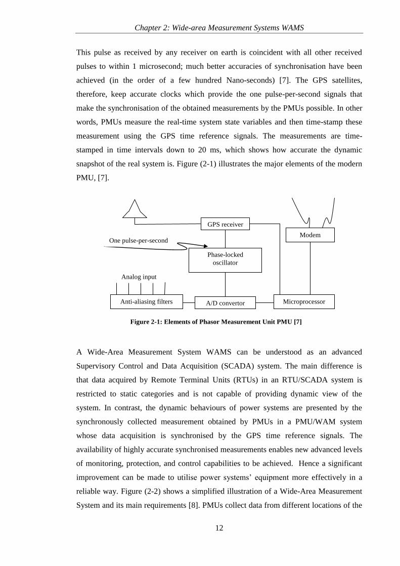
This pulse as received by any receiver on earth is coincident with all other received
pulses to within 1 microsecond; much better accuracies of synchronisation have been
achieved (in the order of a few hundred Nano-seconds) [7]. The GPS satellites,
therefore, keep accurate clocks which provide the one pulse-per-second signals that
make the synchronisation of the obtained measurements by the PMUs possible. In other
words, PMUs measure the real-time system state variables and then time-stamp these
measurement using the GPS time reference signals. The measurements are time-
stamped in time intervals down to 20 ms, which shows how accurate the dynamic
snapshot of the real system is. Figure (2-1) illustrates the major elements of the modern
PMU, [7].
A Wide-Area Measurement System WAMS can be understood as an advanced
Supervisory Control and Data Acquisition (SCADA) system. The main difference is
that data acquired by Remote Terminal Units (RTUs) in an RTU/SCADA system is
restricted to static categories and is not capable of providing dynamic view of the
system. In contrast, the dynamic behaviours of power systems are presented by the
synchronously collected measurement obtained by PMUs in a PMU/WAM system
whose data acquisition is synchronised by the GPS time reference signals. The
availability of highly accurate synchronised measurements enables new advanced levels
of monitoring, protection, and control capabilities to be achieved. Hence a significant
improvement can be made to utilise power systems’ equipment more effectively in a
reliable way. Figure (2-2) shows a simplified illustration of a Wide-Area Measurement
System and its main requirements [8]. PMUs collect data from different locations of the
Figure 2-1: Elements of Phasor Measurement Unit PMU [7]

Chapter 2: Wide-area Measurement Systems WAMS
13
power system network (Data Acquisition). The acquired data is synchronised using
accurate synchronising signals provided by the GPS satellites (Data Synchronisation).
The synchronised data is then transmitted to control centres (Data Transmission) where
decisions regarding the operation and control of the power system are been made
(Control Actions Deployment).
GPS
Satellite
Transmission
Network
PMU
PMU
PMU
Control Centre
PMU
Synchronising Signals
Data Acquisition
Data Transmission and Control
Actions Deployment
Figure 2-2: A simplified WAMS architecture [8]
The advantages of PMU/WAM based systems over the RTU/SCADA systems include
the following [9, 10]:
High-speed data acquisition with a unified time-stamp and high-speed data
transfer capabilities.
Availability of direct measurements which are time-stamped in time intervals of
10-20ms [11].
Availability of wide area dynamic system view.
Availability of dynamic measurements and representation of events encountered
by power systems.
As a result of the availability of an accurate wide-area representation of power system
networks, coordinated and optimised control schemes as well as adaptive relaying in
coordination with local protective devices, which all are aimed for stable, reliable and

Chapter 2: Wide-area Measurement Systems WAMS
14
secure operation of power system networks, become viable and possible to be
developed.
2.2. WAMS Applications in Power Systems
Traditional power systems’ control and protection schemes are, in general, based on
local system information. The main drawbacks of such systems are the inappropriate
system dynamic view and the absence of coordination between local controllers and
decentralised control and protection devices [12]. However, phenomena that threaten
the stable and secure operation of power systems are of a widespread nature (i.e. the
effect of an event disturbance that may cause unstable operation behaviour in one part
of the network can propagate and affect other parts of the network far away from the
origin of the event). This implies that it is difficult to maintain the system stability and
security on the whole if only local measurements are employed in the designing of the
control and protection schemes [13]. With the rising complexity in today’s power
systems, a promising way of enhancing and utilising the operation, control and
protection tasks is to provide a system-wide control and protection schemes,
complementary to the conventional local control and protection strategies. It is
understood that predicting or preventing all events that may cause deterioration of stable
operation conditions of power systems, or may even lead to power system collapse, is
not possible. Nonetheless, a wide-area monitoring and control system that provides
reliable and optimised coordinated control actions is able to mitigate or prevent large
area disturbances. The main advantages which can be accomplished through
incorporating wide-area based monitoring and control systems, using WAMS
applications in the area of power systems operation and control, include:
Enhanced utilisation of power systems through well-designed and well-
coordinated control actions.
Operation closer to the limit through flexible relaying schemes.
Early recognition as well as proper corrective measures of large and small
instabilities phenomena that may be encountered by power systems.
Fewer load interruption events, thus improvement of supply security and system
reliability.

Chapter 2: Wide-area Measurement Systems WAMS
15
To be able to design effective control and protection schemes that ensure stable
operation of power systems, it is important to understand the type, size and nature of
phenomena that may be encountered by these systems, and therefore, need to be
counteracted. In many cases, problems faced by power systems are formulated in
general terms such as “protection against major contingencies” or “counteracting
cascaded outages”. In order to address these problems, there is a need to classify them
and break them down into physical phenomena that can be mitigated by designed
control and protection schemes. Generally, those physical phenomena include control of
and protection against [8, 14]:
Transient angle instability
Small signal angle stability
Frequency stability
Short-term voltage stability
Long-term voltage stability
Cascading outages
For stable, secure and reliable operation of modern power systems, well-designed robust
systems have to be designed so as to arrest the impact of each of the aforementioned
phenomena on power system networks. PMU/WAMS systems can be utilised in many
aspects of monitoring, control and protection against such phenomena. Control and
protective algorithms can be designed based on WAMS applications to provide proper
measures that ensure systems stability.
WAMS applications to power systems can be recognised in three main areas:
Protection, Control, and Monitoring [1]. A number of these applications are starting to
evolve in many power systems around the globe. A good example are those being
deployed in China [15].
2.2.1. Protection
One of the promising applications of WAMS in the area of power system protection is
the possibility of developing adaptive protection schemes. Adaptive protection is a
protection philosophy which permits and seeks to make automatic adjustments in

Chapter 2: Wide-area Measurement Systems WAMS
16
various protection functions so as to allow better performance of the protection scheme.
In contrast, conventional relaying is realised by compromised settings of protection
relays, which are reasonable for many alternative conditions that may exist in a power
system. This, however, implies that these settings may not be the best for any one
specific condition. Therefore, a protection system that is capable of online setting
reconfiguration based on a dynamic view of system operating conditions will
significantly improve the performance of the protection function. An adaptive
protection scheme may include various protection functions, such as:
Identification of fault location based on WAMS
Adaptive online adjustment of relay settings based on wide-area information
Adaptive back-up protection based on WAMS
With a global view of system conditions, wide-area based protection schemes can be
implemented to enhance power systems’ response to disturbances by assuring that
protective actions and faulty equipment/circuit disconnections are formulated precisely
in an optimized way. Wide-area based protection; however, is beyond the scope of this
research.
2.2.2. Control
As for protection schemes, wide-area synchronised measurement technology offers a
unique opportunity to utilise wide-area system information in the design of control
schemes that are aimed to enhance system performance and guarantee system stability.
Generally speaking, oscillatory stability, often referred to as the issue of power system
oscillations, is causing a rising concerns for system operators. This is due to increasing
interconnections between utilities and increase in the amount of power transfer across
these interconnections [16]. This phenomenon is classified, according to the
IEEE/CEGRE Joint Task Force on Stability Terms and Definitions [6], as small signal
rotor angle stability1. The impact of this phenomenon on the whole system can be
significant as it may lead to limit the amount of power transfer between regions and, if
not damped properly, can cause the collapse of the entire system. Hence, damping of
1 This will be discussed further in chapter 3

Chapter 2: Wide-area Measurement Systems WAMS
17
power system oscillations between interconnected areas is an important controlling task
for secure and stable operation of power systems.
Power system oscillations are of two modes [6]. Local modes, which is the notion of
the oscillation of one generator or one plant in an area against the rest of the system, and
inter-area modes, which are associated with the oscillations of groups of generators or
plants in different areas against each other. Local modes of oscillation are largely
determined and influenced by local area states and, in most cases, control measures in
the form of local conventional power system stabilisers PSS [17] can be sufficient
enough to deal with them and provide the required damping for the oscillations.
However, oscillations in the form of inter-area modes are not as highly observable and
controllable using local system observations as local modes. As a result, control
measures for inter-area modes of oscillations are rather complicated and, therefore,
concerns arise in this area giving the rising complexity of power systems. In addition,
local conventional controllers, such as PSSs, have fixed parameters that, in most
practical cases, are determined based on linearized system models and are tuned in non-
optimum ways to deal with both modes of oscillations. Hence, alternative techniques to
provide damping for inter-area oscillations become a necessity for maximum utilisation
of power systems.
Since inter-area oscillations are more of a wide-area phenomenon, wide-area signal
measurements provided by WAMS can be utilised to provide appropriate remote signals
to optimally located damping devices, such as PSS or FACTS (Flexible AC
Transmission Systems) controllers, to damp the oscillations. Thus, allowing maximum
utilisation of interconnections without violating stability, security and reliability
constraints. Applications of WAMS for control of power system oscillations can be
categorised based on three control design techniques which are [18]:
De-centralised controllers
Centralised controllers
Multi-agent controllers
A further discussion of these techniques is provided in chapter 3.

Chapter 2: Wide-area Measurement Systems WAMS
18
2.2.3. Monitoring and Recording
Keeping an eye on power systems, by constantly monitoring the changes in their
operating conditions, is an important task for operation and control of such highly non-
linear dynamic systems. The implementation of PMU/WAMS technologies in power
systems significantly improves the possibilities for monitoring and managing power
system dynamics [1, 15]. PMUs installed in selected locations of a power system
provide important information about different system states, such as voltages, currents,
active and reactive powers, all of which are timely-stamped based on GPS time
reference signals. The dynamic system view obtained by WAMS provides improved
monitoring capabilities that allow system operators to utilise the existing power systems
more efficiently. Improved information about systems conditions allows fast and
reliable emergency actions, which reduce the need for relatively high transmission
margins required by potential power system disturbances.
Besides the improvement in the monitoring and recording of power system dynamics,
WAMS enables the improvement of the task of state estimation [1]. The inaccuracy and
delays of traditional SCADA systems can be eliminated by PMU/WAMS based
systems. The accurate time-stamped data provided by PMUs can be used as the basis for
improved state estimations; thus, allowing instant calculations of system states. Based
on fast, accurate and reliable state estimation, a variety of online system stability indices
regarding different stability phenomena can be made available for system operators. As
a result, the task of optimised operation of existing power systems can be fulfilled.
The focus of this research project will be on the application of WAMS technologies in
the area of power system control. The aim is to develop control schemes that are based
on WAMS techniques so as to enhance the performance of power systems and allow
higher amounts of power transfer across transmission interconnections. In the next
chapter one of the rising concerns, which is believed to cause limitation in the amount
of power transfer across transmission lines in interconnected power systems, is
addressed. These concerns are related to the issue of power system oscillations and their
impact on the stable operation of power systems.
Chapter 2: Wide-area Measurement Systems WAMS
19
2.3. Summary
An overview of wide-area measurement systems (WAMS) and their applications in
power systems is introduced in this chapter. The basic elements and architecture of
WAMS are illustrated indicating their advantages over traditional measurement and
monitoring tools in the form of RTU/SCADA systems. A general view of WAMS
applications in the area of monitoring, protection and control of power systems is
introduced. The application of WAMS in power system control is the focus of the rest
of the chapters of this thesis. In the next chapter (chapter 3), the main focus is power
system oscillation and the applications of wide-area based control damping measures.
Chapter 3: Power System Oscillations and Control Measures
20
Chapter 3: Power System Oscillations and Control Measures
3.1. Overview
Power system oscillations are phenomena inherent to power systems. They are often
referred to as electro-mechanical oscillations that occur between interconnected
synchronous generators in multi-machine power systems [19]. Historically, oscillations
in power systems were observed as soon as synchronous generators were interconnected
via transmission networks to provide electrical power to remote areas that have no
generation capabilities. Interests in interconnecting power system utilities through
transmission networks started in the 1950s and 1960s after realising the possibilities of
achieving reliability and economic benefits. However, in many cases, high amounts of
power transfer across the transmission networks were constrained because of low
frequency growing oscillations that are initiated by changes in the operation conditions
of power systems [20]. The stability of these oscillations is a compulsory requirement
for stable and secure operation of power systems.
As mentioned in section 2.2, to provide effective control strategies, it is important to
classify operation difficulties and problems encountered by power systems into physical
phenomena so that they can be mitigated and, hence, controlled and counteracted. The
phenomenon of power system oscillations is classified, according to the IEEE/CEGRE
Joint Task Force on Stability Terms and Definitions [6], as small signal generators’
rotor angle stability. This category of stability is concerned with the ability of power
systems to maintain synchronous operation following small changes in their operation
conditions and it is, in most cases, a problem of insufficient damping of low frequency
oscillations [21]. The phenomenon is further broken down into two modes of
oscillations; one is of a local nature, whereas the other is of a global or wide-area nature.
These modes are:
Local Modes of Oscillations: These modes are associated with the oscillation of a
single generator or a single plant in the power system with respect to the other
generators in the system. The oscillation frequencies of these modes are in the range

Chapter 3: Power System Oscillations and Control Measures
21
of 0.7 to 2.0 Hz [19],[21]. The characteristics of these oscillations are observable by
local measurements of local area states where oscillations occur. In practice,
effective control measures that are relatively simple can be developed to damp these
oscillations. A typical control measure is a conventional Power System Stabiliser
PSS that provides supplementary control signal to generators’ excitation systems.
The effect of the control signals provided by PSS may be sufficient enough to solve
the problem and provide proper damping for the local oscillations.
Inter-Area Modes of Oscillations: These modes are associated with the oscillation of
groups of generators or groups of plants against other groups. The oscillation
frequencies of these modes are in the range of 0.1 to 0.8 Hz [19],[21]. The
characteristics of these modes are complex and far more different from those of
local oscillations modes. The effectiveness in damping these types of oscillations is
limited because they are not as highly observable and controllable in local system
information as those of local modes. Inter-area oscillations are global problems
caused by the interactions among large groups of generators and can have a
widespread effect. The absence of a global view of the entire system makes it
difficult for local controller, which are effective in damping local oscillations, to
provide adequate damping for inter-area oscillations.
In today’s power systems and from an operation and control point of view, inter-area
oscillations seems to be the most problematic stability aspect due to increasing
interconnections between utilities. With increased pressure on utilities to maximise the
use of their existing networks and push more power through the interconnections, rising
concerns about inter-area oscillations form a challenging barrier that can prevent
utilities from achieving such goals. Hence control schemes that overcome this issue and
provide proper damping for these oscillations are desirable.
3.2. Wide-Area based Control Schemes for Power System Oscillations Damping
As mentioned in chapter 2 section 2.2, the applications of wide-area measurement
systems for wide-area based stability control are realised by three categories of
controllers’ design philosophies which are; decentralised controllers, centralised

Chapter 3: Power System Oscillations and Control Measures
22
controllers and multi-agent controllers. The aim of the three categories is providing
tools by which power systems are operated in such a way where system stability is
retained and system oscillations are damped properly. Further discussion of these
control strategies and an investigation of a number of techniques that have been
developed based on these control strategies are included in the following subsections.
The basic structure of decentralised and centralised control schemes is shown in Figure
(3-1) bellow [22]. The green part illustrates the traditional framework of decentralised
controllers whereas the red part shows that of centralised control strategies. The basic
structure of multi-agent based controllers is shown later in Figure (3-6) [22].
Control Centre
Local
device
Local
device
Local
device
Local
device
Local Controller
Power System Connections
Flow of signals
Flow of information
Feedback signal
Control signal
Feedback signalControl signal
Control Centre
Figure 3-1: Framework of centralised and decentralised control schemes [22]
3.2.1. Decentralised Control Strategies
The function of decentralised control schemes is realised by local controllers that are
installed to act upon local devices and provide control actions to alter the status of these
local devices to meet the requirement of the specific operation condition (as shown by
the green part in Figure (3-1)). Traditional decentralised controllers are designed based
on locally available feedback signals that provide direct information about the local
devices to which these controllers are connected. The local feedback signals are

Chapter 3: Power System Oscillations and Control Measures
23
processed by the controller and based on the objective function of the controller, control
signals are determined and sent to the local device to adjust its operational status. The
drawbacks of these traditional schemes is that the actions of the local controllers
consider only the status and requirement of the local devices and do not take into
account the status and needs of other local devices in the network. Considering that, in
many cases the requirement of other local devices can be significantly influenced by the
action of a local controller, it is clear that under such schemes of decentralised
controllers the effectiveness of local controllers is constrained. An improvement of such
schemes can be made if decentralised controllers are designed so that they can have a
wider view of the system status and be able to support each other. WAMS applications
in this area provide the required tools to improve the performance of these local
decentralised control schemes. Such an improvement can be made possible by
providing additional global and remote signals to the existing local controllers. Hence,
global phenomena such as inter-area oscillations can be counteracted more effectively.
Interests in enhancement damping capabilities of local decentralised controllers based
on global signals started in 1990s. A good example of this is the proposed method
introduced in reference [23]. The proposed controller is, basically, a two level Power
System Stabilizer PSS. The objective function of the first level of control is to damp the
local mode in the area where the controller is installed using generator rotor speed
signals as a local feedback input signals to the controller. The objective function of the
second level of control is to provide damping for inter-area oscillatory modes using
additional global feedback signals. Two types of global feedback signals are suggested;
tie-line active power and speed difference signals. Location of the two level PSS, input
signals selection, and tuning of the controller parameters are obtained based on modal
analysis techniques using participation factors or transfer function residues. In the same
research, the same principles of two levels of control are also applied to SVC (Static
VAR Compensator) devices located in the middle of the transmission line connecting
two oscillating groups. The two level PSS is shown in Figure (3-2).

Chapter 3: Power System Oscillations and Control Measures
24
Coordinator
PSS2j
PSS2i
Genj
PSS2j
Geni
PSS2i
Ugj
Ugi
Ptie12
Area 2 Area 1
)(
12
ji
tie
or
P
U1j U1
i
+
++
+j i
Figure 3-2: Two-level PSS design architecture [23]
Reference [24] adopts a decentralised / hierarchical approach to design a wide-area
signal based PSS that provides the required additional damping for inter-area oscillation
modes in the Hydro-Quebec’s transmission system. The design approach uses the state
space system identification techniques. Once the state space model of the system is
obtained, observability and controllability measures are computed from which PMUs
remote signals spread over coherent areas are selected. Again, the proposed PSSs in this
research have two control levels. The first is a traditional speed sensitive local loop
operating in the traditional way [17] whereas the second level is a WAMS based global
loop that uses a single differential frequency signals between two selected areas. Since
the remote feedback loops are built on top of an existing decentralised control system,
the design approach, therefore, results in a decentralised / hierarchical structure. The
general architecture of the control system is shown in Figure (3-3).
A methodology to compare wide-area and local signal based supplementary control of
shunt FACTS devices for improved damping of inter-area oscillation modes is
presented in [25] through numerical simulations of a three-area test system and
generalised on a large study system using a revised Hydro-Quebec network. Again, the
results suggest that wide-area based damping controllers have obvious advantages.
However, it also suggest that local control can be quite effective even at moderate gains
and, therefore, it is recommended that in a decentralised / hierarchical design
approaches, one should always start with local control loops and then add wide-area
control loops as needed, depending on the system requirements.

Chapter 3: Power System Oscillations and Control Measures
25
PMU#1
PMU#2
PMU#q
SCADA
Global PSS #1 Global PSS #p
Local PSS #pLocal PSS #1
~ ~
Excitation Excitation
Gen
#1
Gen
#p
Remote Measurements
Real-time monitoring
Figure 3-3: General architecture of a decentralised / hierarchical PSS design [24]
Test results for the aforementioned attempts show that a major improvement in the
stability of power systems using wide-area measurements as an additional input signals
for decentralised damping controllers can be achieved. However, focus needs to be put
when designing such wide-area based controllers regarding signals transmission time
delays as time delays, if not considered in the design process, can have a significant
impact on the system stability.
3.2.2. Centralised Control Strategies
The function of traditional centralised control schemes is realised by centralised
controllers which are located in control centres. A centralised controller receives
feedback signals from all local devices in a power system and sends control commands
to these devices (as shown by the red part in Figure (3-1) above). This indicates that a

Chapter 3: Power System Oscillations and Control Measures
26
large amount of information is needed to be transmitted to the control centres where this
information is processed and then control measures are taken. Hence a significant time-
delay is involved, which implies that traditional centralised control methods applied to
power systems are for the control of slow process and are not suitable for fast on-line
power systems control. The advantages of WAMS in providing fast transfer capabilities
of synchronised measurements open a new path by which centralised control can be
enhanced significantly. Examples of attempts to do so are described briefly next.
A two level hierarchical structure is introduced in [26] to improve the stability and
oscillation damping in multi-machine power systems. The proposed structure consists of
a local controller for each generator at the first level helped by multivariable central
controller at the secondary level. The secondary-level controller uses remote signals
from all generators to produce decoupling control signals that improve the performance
of the local controller. The local controller uses only local signals to damp local
oscillation modes. The proposed hierarchical controller structure is shown in Figure (3-
4).
Local
Controller
Local
Controller
Wide-Area
Controller
~
~
Remote Signals
Local Signals
Local Signals
Gen # 1
Gen # n
Figure 3-4: The hierarchical controller structure [26]
In the proposed scheme, problems of voltage regulation and rotor oscillations damping
are addressed simultaneously. The second-level controller continuously adapts its
parameters through a gain scheduling algorithm and provides additional control signals
to local controller based on wide-area system view. In the absence of the global signal
from the centralised wide-area controller, local controller still can perform in a
traditional way. Test results show that the performance of local controllers is
considerably enhanced by the secondary control action and system stability is improved
in presence of severe operating conditions.

Chapter 3: Power System Oscillations and Control Measures
27
A centralised control system for damping power system inter-area oscillation using
wide-area measurement is presented in [27]. Again, the proposed scheme consists of
two levels of control. The first level is fully decentralised and consists of conventional
PSSs. The second level is centralised and provides supplementary damping signals that
are sent to local devices in addition to the first level of control. The general structure of
the centralised wide-area damping control system is shown in Figure (3-5).
Excitation
System
Excitation
System
AVR
PSS PSS
AVR
GenGen
Wide-Area Damping Controller
(WADC)
PMU PMU
++
Wide-area control
signals
Wide-area control
signals
VrefV
ref
Figure 3-5: General structure of a wide-area centralised damping control system [27]
In the proposed scheme, geometric measures of controllability/observability are used to
select the most effective stabilizing signals and control locations. Line power flows and
currents are found to be the most effective input signals to the controller. The
application of Linear Matrix Inequalities (LMI) is used for tuning and optimisation of
the controller. The test results show that the use of linear, continuous methods to design
a controller, although very powerful, requires a considerable tuning, testing and further
development when implemented in nonlinear discontinuous real systems such as power
networks. However, the designed controller shows promising results in providing

Chapter 3: Power System Oscillations and Control Measures
28
effective damping for power system oscillations as well as obtaining robust control
performance.
A multiple-input, single-output (MISO) controller is designed in [28] for a Thyristor-
controlled series capacitor (TCSC) to improve the damping of inter-area oscillation
mode in power systems. The stabilising signals are obtained from remote locations
based on observability of critical inter-area oscillation modes. The design of the
centralised controller is formulated as a multi-objective optimisation problem in the
LMI (Linear Matrix Inequalities) framework. Using both, Eigen values analysis and
time domain simulation, the robust performance of the proposed controller has been
verified. It concluded that, because the number of inter-area oscillation modes in
practical power systems is often much larger than the number of available control
devices, centralised control design approach using global signals is, therefore, one of the
potential options for stability enhancement and utilisation improvement.
3.2.3. Multi-agent Control Strategies
Coordination of control measures taken by multiple decentralised local controllers is a
significant task that can play a significant role in the enhancement of the overall
performance of modern power systems. Most decentralised control schemes exist today;
however, rely on non-adaptive coordination techniques that are determined by off-line
coordination methods. Such techniques do not consider on-line changes in the operating
conditions of power systems. As a result controllers lack the ability to adapt to the
variations of power system operating conditions and, therefore, are unable to function
effectively under unexpected circumstances. With the rising complexity of power
systems, there are needs to utilise these local controllers more efficiently. Hence, more
effective coordination between decentralised local controllers is desirable. Coordination
should rely on on-line exchange of information in such a way that controllers support
each other and take into consideration the status of other nearby devices, instead of
focusing their control actions only on the status of local devices. Such coordination
techniques have the advantages of flexibility, autonomy intelligence and on-line
adjustment capability, all of which can be applicable by the applications of multi-agent

Chapter 3: Power System Oscillations and Control Measures
29
technology in the area of power system operation and control [29],[30]. General
framework of multi-agent based coordinated controllers is shown in Figure (3-6) [22].
Local Controller
Local
device
Local Controller
Local
device
Local Controller
Local
device
Local
device
Control Centre
Feedback signal
Feedback signal
Feedback signalControl signal
Control
signal
Control signal
Communication
Communication
Adaptation
Adaptation Adaptation
guide
guide guide
Power system connection
Flow of signals
Flow of information
Figure 3-6: Framework of multi-agent based controllers [22]
Reference [31] proposes a supervisory level power system stabiliser (SPSS) using wide-
area measurements. The coordination between the proposed SPSS and the local Power
system stabiliser (LPSS) is implemented based on the concept of multi-agent system
theory. In the proposed multi-agent damping control scheme, LPSSs are placed at the
selected generator excitation loops and tuned to damp local oscillation modes. They are
categorised as local agents and remain in the same location throughout their working
lives. The SPSS operates as a software agent that has three main components as shown
in Figure (3-7). These components are; agent communications, fuzzy logic controller
switch and robust control loops. The function of fuzzy logic controller is to switch to
the appropriate robust controller to provide a satisfactory damping for the corresponding
system operation conditions. The controller embedded in the SPSS control loop is
designed based on H∞ controller using selected wide-area measurements. The use of H∞
optimization method to design the controller is adopted to accommodate power system
nonlinear dynamic performance and model uncertainty.
The additional damping signals produced by the SPSS are sent to local machines to
provide damping for system oscillation through the excitation systems of these local
machines as shown in Figure (3-8).

Chapter 3: Power System Oscillations and Control Measures
30
Agent Communication
Rule Base
Robust Controller LoopsFuzzy Logic Switch
)( basedH
Communication
Network
SPSS
Figure 3-7: Components of SPSS [31]
Figure 3-8: Conceptual input/output scheme of SPSS [31]
In the proposed techniques signal transmission delays are not taking into account. Also
the control loops design is determined off-line which may cause issues when the
operating conditions change significantly. Nonetheless, the test results of the technique
show that the proposed design can effectively damp system oscillations under range of
operating conditions.
3.3. Power System Oscillations and the Concept of Coherent Clusters
As discussed in section 3.1, electromechanical oscillations are inherent phenomenon to
power systems that is highly related to the complex dynamics of highly non-linear
SPSS Remote Signals
LPSS Local Signals
Voltage
Regulator
Generator
Excitation
System
Gen+V
tV
ref
-

Chapter 3: Power System Oscillations and Control Measures
31
systems. However, the frequency of these oscillations and the number of synchronous
machines involved in any electromechanical oscillatory mode depend on the structure of
the power system network. Generally speaking, low frequency electromechanical
oscillations are more likely to be observed when geographically dispersed
generation/load areas are connected to each other via relatively weak transmission lines
compare to the rest of the transmission network [32]. The weak interconnections can,
sometimes, be obvious when, for example, two independent power system networks are
interconnected through a single tie-line. However, for systems which have been
interconnected for a period of time, electromechanical oscillations may appear due to
stressed operation conditions and increase in power transfer across the transmission
network. In such cases, identifying critical transmission lines and critical areas from
which oscillatory system behaviour may originate becomes a vital task for stability
studies and control of power systems.
Experiences and observations of operation of power systems networks conclude that,
when a stressed power system experiences a disturbance or a change in its operation
conditions, electromechanical oscillation between interconnected synchronous
generators may appear. Following a change in their operation conditions, power systems
tend to oscillate coherently with groups of generators in a specific area of the power
system behaving coherently in low frequency electromechanical oscillations [20]. Those
groups of coherent generators are separated, yet connected, to other groups of coherent
generators by weak transmission lines.
These observations bring about the concept of Coherent Clusters or Critical Clusters
(CC). A Coherent Cluster of synchronous generators can be defined as the group of
generators that behaves similarly or have similar response characteristics to changes in
the operation conditions of a power system in which they operate. The identification of
these clusters is of importance in the study of power system stability and the design of
the appropriate countermeasures that aim to maintain system stability. A number of
approaches have been proposed and applied to identify the coherent clusters in multi-
machine power systems, some of which are discussed in the next section (section 3.4).

Chapter 3: Power System Oscillations and Control Measures
32
3.4. Identification of Coherent Clusters in Power Systems
Considerable amount of research has been devoted to identify coherent clusters of
synchronous generators in multi-machine power systems. Most of these research pieces
differ in their approach in how to obtain or identify the coherent clusters. For example,
coherency-based approaches have been, in the past, proposed to aggregate those
generators in certain coherent groups, which have similar responses to a system
disturbance, into dynamic equivalent subsystems for the purpose of developing reduced
dynamic equivalents for large interconnected power systems [33],[34],[35]. In these
approaches, the coherent group is replaced by a single generator which has dynamic
parameters identical to those of each generator in the group, but which has a rating
equivalent to the total group rating. Thus, reduced dynamic models for large power
systems are obtained. However, from an operation and control point of view, the
identification of coherent clusters is of importance for proper understanding to power
system stability studies and for the design of control schemes that aim to enhance the
overall system performance.
Early research [36] based on the Extended Equal Area Criterion EEAC [37] focuses on
splitting the multi-machine power system into two groups of machines; one group forms
the critical machines and the other one consists of the remaining machines. The critical
machines are those responsible for loss of synchronism in a power system following a
disturbance and therefore, coherent in their response to the disturbance. The aim of this
approach is to evaluate the system’s stability margin corresponding to a given
disturbance. A different approach introduced in [38, 39] uses the line transient potential
energy to identify vulnerable transmission segments and clusters of critical machines.
This approach considers the phenomenon on the power system network rather than the
group of machines. The basic concept is that, following the clearance of a fault, the
increase in the generator rotors kinetic energy will be converted into potential energy
and distributed over the whole network. If the converted energy can be absorbed by the
network, the system will remain stable; otherwise instability may occur and there will
be a corresponding unstable cut-set. Based on this concept, an index is derived to
identify the critical cut-set (critical lines). According to this index, the lines are sorted in
ascending order and then removed one by one until an island is formed. This island
includes the coherent or critical machines and it identifies the critical clusters.

Chapter 3: Power System Oscillations and Control Measures
33
Giving the advantages of WAMS, identifying coherent clusters of generators based on
wide-area signal measurements plays a significant role in the design of wide-area based
stability controls. Research aimed to identify coherent clusters based on PMUs
measurements has evolved recently, some of which is discussed briefly next.
Reference [40] discusses a way of clustering generators in coherent groups based on
phasor measurements obtained by PMUs. The clustering technique uses Discrete
Fourier Transform (DFT) analysis for estimated internal voltage phasor of all generators
to derive indices that are used to aggregate those generators into coherent groups. A
method suitable for real time coherency identification is introduced in [41]. Fourier
analysis are applied to the monitored generator speed signals in [41]. The basis of this
method relies on the theory that during normal operation of synchronous generators,
their rotor speed deviation is zero. During a disturbance, the rotor angle will change to
meet the new system condition. This change in the operating point appears as a
developed oscillation which can be seen as a speed deviation on the rotor speed signals.
Based on these facts and by monitoring the generator speed and applying Fourier
analysis, the fundamental speed will be recognised by the zero frequency spectral
components while the speed deviation is reflected by the nonzero frequency
components. Furthermore, the phases of the dominant nonzero frequency components
of all generators are also determined, and by comparing them, the generators coherency
can be acquired. Another technique based on wide-area signal measurements is
developed in [42]. The method introduces a hierarchical clustering technique of (N)
generators into coherent groups based on wide area measurements. The clustering
method can produce any number of groups between 1 and N. Then a single generator is
selected to represent each group. The rotor frequencies of the representative generators
are used to identify the cluster with the largest initial swing; hence, identifying the event
location (i.e. finding the most likely group from which an event originates). The method
uses a weighted sum squared error (WSSE) objective function to aggregate the
generators two clusters at a time starting from each generator as a cluster itself.
Choosing which two clusters to merge is based on the well-known Ward’s method.
The main drawbacks of the previously described techniques are that they do not
consider wide range of operating scenarios for power system networks. Instead, the

Chapter 3: Power System Oscillations and Control Measures
34
identification of the coherent clusters is obtained based on system response to
predefined, limited contingencies. Due to the fact that clusters configuration may be
significantly influenced by the type, size, and nature of the encountered disturbance, a
technique that can take into account as many events that lead to oscillatory behaviour of
the machines as possible is desirable. Such clustering technique will assure the accuracy
in the clustering configuration for the system regardless of variation in the operating
scenarios.
3.5. Summary
The phenomena of power system oscillations and its threatening impact to the stable
operation of power systems are presented in this chapter. A number of wide-area based
control schemes developed to enhance power system oscillation damping capabilities is
reviewed and summarised based on the adopted control strategy (i.e. centralised control
strategy, decentralised control strategy and / or multi-agent control strategy). Also the
concept of coherent clusters (CC) which is related to the oscillations of coherent groups
of synchronous generators in multi-machine power systems is introduced. A number of
techniques developed to identify coherent clusters in power systems are summarised in
an attempt to identify the drawbacks of such techniques and develop a new algorithm to
determine the coherent clusters in large power systems. In chapter 4, a new technique to
identify coherent clusters of synchronous generators in multi-machine power systems is
proposed. The merits of the proposed method are the following:
The clustering technique is based on wide-area signal measurements; hence it is
suitable for implementation in WAMS based monitoring and control system.
A new technique is proposed to account for the effect of different types of events on
the clusters configurations. Thus, the accuracy in the clustering is assured.

Chapter 4: A Novel WAM based Technique to Identify Coherent Clusters in Multi-
machine Power Systems
35
Chapter 4: A Novel WAM based Technique to Identify
Coherent Clusters in Multi-machine Power Systems
4.1. Overview
The Coherent Clusters are previously defined as the groups of generators that behave
similarly or have similar response characteristics to changes in the operation conditions
of a power system in which they operate. Changes in the operation conditions of a
power system may, sometimes, cause oscillations of groups of generators against other
groups. The oscillations characteristics are highly observable in generators rotor signals
such as generators rotor speed deviation signals or generator rotor angle signals. If
quantities that describe the dynamic behaviours of generator rotors during system
oscillation are available, coherency measures can be derived to identify the coherent
clusters.
Recent research suggests that generator rotor angle measurements can be obtained using
Phasor Measurement Units (PMUs) technologies [42],[43],[44]. Therefore synchronised
measurements of generator rotor frequencies using a wide-area measurement system are
applicable. Hence an algorithm that identifies coherent generators based on these
measured quantities can be implemented in a wide-area based stability control scheme.
In this section, an agglomerative hierarchical clustering algorithm is proposed to group
any number of generators in a given multi-machine power system into coherent clusters
based on simulation data. The clustering is based on coherency measures obtained from
the time-domain responses of all generators following a disturbance. The main
advantage of this proposed method over the other previously described wide-area based
methods lies in the proposed technique introduced to account for as many events that
lead to oscillatory behaviour of the machines as possible. Thus it is assured that the
obtained cluster configurations are the most likely ones to be formed under any type of
disturbances.

Chapter 4: A Novel WAM based Technique to Identify Coherent Clusters in Multi-
machine Power Systems
36
4.2. Methodology
The proposed agglomerative hierarchical clustering algorithm is to be applied for a data
set consisting of the time-domain responses of all generators during and following a
disturbance. A typical time domain response of a group of interconnected synchronous
generators to a disturbance or a change in the operation conditions of the power network
is similar to the one shown in Figure (4-1) bellow. The dynamic quantities being
observed in Figure (4-1) are the rotors’ speed deviation signals following a system
disturbance. As can be seen, prior to the event, speed deviations of all generator rotors
are Zeros indicating stable operation of the generators where electrical power is being
delivered at constant rotor speeds and constant rotor angles. Following a disturbance,
the rotor angles move to meet the new operating condition. These changes in the
operating points result in developed oscillations which can be seen as speed deviation
on the rotors’ speeds. The oscillations continue for a period of time and then decay, if
there are enough damping forces in the system.
Rotor Speed Deviation
50403020100 [s]
0.0375
0.0250
0.0125
0.0000
-0.0125
-0.0250
-0.0375
Time (Seconds)
Rotor Speed Deviation (Hz)
DIg
SIL
EN
T
Figure 4-1: Typical response of generators group (rotors speed deviation) to a system disturbance
Considering a system consists of (Ng) generators, the generators’ rotor speed deviation
(∆ω) can be taken as the basic time-series data set to represent the dynamics of all the

Chapter 4: A Novel WAM based Technique to Identify Coherent Clusters in Multi-
machine Power Systems
37
generators in the power system. For a given disturbance or event (e) and for a response
time (T), the data set to be clustered can be presented by the following matrix.
)()()(
)()()(
)()()(
21
22212
12111
TNNN
T
T
e
ttt
ttt
ttt
ggg
(4.1)
Where:
∆ω: is the rotor speed deviation.
T: is the time of the event simulation.
Ng: is the number of generators.
From such a data set, coherency measures between generators can be identified.
4.2.1. Coherency Identification
From the data set matrix, coherency between each pair of generators can be obtained by
computing the Euclidean Distance [45] for each pair, as in equation (4.2). The
Euclidean distance reflects the dissimilarity between each pair of generators in their
response to the encountered disturbance. And for this reason, it will be referred to as the
dissimilarity coefficient.
T
tt
jiij ttd1
2))()(( (4.2)
Where:
ijd : is the dissimilarity coefficient between generator i and generator j .
)(ti : is the thi generator speed deviation at the time instant ( t ).
)(tj : is the thj generator speed deviation at the time instant ( t ).
Based on dissimilarity coefficients matrix obtained by (4.2), the pairs with the smallest
distance are selected to be merged into one cluster. Then the dissimilarity matrix is

Chapter 4: A Novel WAM based Technique to Identify Coherent Clusters in Multi-
machine Power Systems
38
updated by calculating the distances between the new clusters. Various clustering
techniques differ in how to update the dissimilarity matrix. Hierarchical agglomerative
clustering techniques are integrated into MATLAB and there are different methods
available to compute the updated dissimilarity matrix. The average linkage method is
one of the methods with the best performance and it uses the average distance between
all pairs of objects (generators in this case) in any two clusters as in equation (4.3):
r sN
i
N
j
sjri
sr
rs xxdistNN
d1 1
,1
(4.3)
Where:
rsd : is dissimilarity coefficient between cluster (r) and cluster (s).
rN and sN : are the number of objects (generators) in cluster (r) and (s) respectively.
sjri xxdist , : is the distance between object (xi) in cluster (r) to object (xj) in cluster (s).
4.2.2. The Events’ Effect on the Clustering
It is well established that the response of a generator to a disturbance depends on the
type of event or disturbance (i.e. multi-phase/single phase fault, line trip, event of load,
etc.) as well as on the location of the event. Therefore, the clustering process may be
influenced by the configuration of events. It is also well known that the machine inertias
are typically proportional to the active power output of the machine [46]. If the
generators’ active power output during an event disturbance is available, the influence
of that specific event can be taken into consideration. Generators’ active power outputs
also follow a pattern of oscillation behaviours following a system disturbance similar to
those shown in Figure (4-1) for the speed deviation. A typical response is similar to the
one shown in Figure (4-2) which shows active power outputs of group of generators
following a system disturbance.

Chapter 4: A Novel WAM based Technique to Identify Coherent Clusters in Multi-
machine Power Systems
39
50403020100 [s]
1200.00
1000.00
800.00
600.00
400.00
200.00
0.00
Active Power MW
Time (seconds)
DIg
SIL
EN
T
Figure 4-2: Active power outputs of generators group during a system disturbance
Equation (4.1) gives a time-series data set that describes the responses of (Ng)
generating unit to a specified event (e). For the same event, a time-series matrix of
generators’ active power output can be obtained from the time domain simulation for
the same time period (T), as in equation (4.4).
)()()(
)()()(
)()()(
21
22212
12111
TNNN
T
T
e
tPtPtP
tPtPtP
tPtPtP
P
ggg
(4.4)
Equations (4.1) and (4.4) are the time-series matrices of generators’ speed deviation and
active power output, respectively, for a specific event (e). For a number of events (m),
an equivalent data set for the speed deviation matrix can be computed taking into
account the weight of each event by considering the active power output of each
generator during each event. The speed deviation of the (ith
) generators at the instant of
time (t) can be computed as an equivalent, considering all events, as follows:

Chapter 4: A Novel WAM based Technique to Identify Coherent Clusters in Multi-
machine Power Systems
40
m
e
i
e
i
e
m
e
i
ei
eq
tP
tPt
t
1
1
)(
)()(
)(
(4.5)
Where:
)(ti
eq : is the equivalent speed deviation of the thi generator at time ( t ).
)(ti
e : is the speed deviation of the thi generator at time ( t ) for the event ( e ).
)(tPi
e : is the active power output of the thi generator at time ( t ) for the event ( e ).
m : is the number of events.
The equivalent speed deviation data set matrix is shown in equation (4.6). The data set
included in this matrix is then used in the clustering algorithm to compute the
dissimilarity matrix and to form the cluster tree, equations (4.2) and (4.3).
)()()(
)()()(
)()()(
21
2
2
2
1
2
1
2
1
1
1
T
N
eq
N
eq
N
eq
Teqeqeq
Teqeqeq
eq
ttt
ttt
ttt
ggg
(4.6)
Using equations (4.1) to (4.6) the clustering algorithm used to group the power system
synchronous generators into coherent clusters is described by the flow chart in Figure
(4-3).

Chapter 4: A Novel WAM based Technique to Identify Coherent Clusters in Multi-
machine Power Systems
41
Perform a number of events for
the given power system
Select the oscillatory cases
Construct the equivalent data set
matrix "Equation (4.5)"
Construct the dissimilarity coeficients
matrix from the equivalent data set
matrix "Equation (4.2)"
Merge the two clusters with the
smallest dissimilarity coefficient
Stop and construct the
cluster tree
Update the dissimilarity
coefficient matrix
"Equation (4.3)"
Final clustering
step
Yes
No
Figure 4-3: Flowchart for the proposed clustering algorithm
4.3. Algorithm Implementation (Software and Simulation)
To acquire the measurements needed by the proposed clustering algorithm, the
DIgSILENT (Digital Simulator for Electrical Network) simulation software is used to
simulate the power system under study. DIgSILENT [47] is a consulting and software
company based in Germany that provides specialised services in the field of electrical
power systems for transmission, distribution, generation and industrial plants. The
software is an integrated power system analysis tool that combines reliable and flexible
system modelling capabilities. It has the capabilities of simulating an arbitrary power

Chapter 4: A Novel WAM based Technique to Identify Coherent Clusters in Multi-
machine Power Systems
42
system network on every time scale, from steady state load flow analysis through to
electromagnetic transient simulation. DIgSILENT provides a basic simulation kernel,
which together with a comprehensive model library and graphical user-definable
modelling system, provides an extremely flexible and powerful platform for solving
power system dynamic problems. Simulation functions available in DIgSILENT
includes; load flow and fault analysis of complete AC/DC network representation, low
voltage network analysis, distribution network optimisation, electromechanical dynamic
simulation, electromagnetic dynamic simulation, Eigen value analysis, protection
analysis, harmonic analysis, reliability analysis, voltage stability analysis, contingency
analysis, power electronic device modelling, and others [47]. In addition, it has a wide
range of built-in detailed and dynamic models of power systems equipment and
controllers including synchronous/asynchronous machines, transformers, excitation
systems and voltage regulators AVRs, generators speed governors, power system
stabilisers, DFIG and full converter wind turbine, etc, all of which make it a very
attractive package for usage.
4.4. Test Systems
Test systems are widely used in power system research studies. There are reasons for
using such test systems instead of using models of practical systems such as the
following:
Scarcity of practical power systems data due to confidentiality.
Dynamic and static data of the systems are not well documented.
Due to the large set of data of real world power systems, calculations of
numerous scenarios can be very difficult.
Lack of software capabilities for handling large set of data. Most educational
softwares have limitations regarding system sizes.
Results from practical power systems are less generic due to the special
arrangements and specific standard for each practical system. Whereas standard
test systems are more generic and mimic the behaviours of real system to a
certain extent.

Chapter 4: A Novel WAM based Technique to Identify Coherent Clusters in Multi-
machine Power Systems
43
For these reasons, a number of standard test cases are documented for research
purposes. The available test cases and commonly systems can broadly be categorised
into transmission test system, distribution (sub-transmission) test systems and
unbalanced distribution systems. In this research work, test systems which are suitable
for studies of power system stability, low frequency oscillatory stability analysis and
studies of new controllers in power system stability are used. For testing the coherency
identification algorithm two standard test systems are used as case studies. Those test
systems are the 16 generator 68 bus test system and the IEEE 39 bus test system.
4.4.1. Case Study 1: 16 generator 68 bus test system
The study system used to test the performance of the proposed algorithm is the standard
16 generator 68-bus system which is a reduced order equivalent model of the New
England / New York interconnected power system. In this system, there are 68 buses
and 16 generation units, interconnected via high voltage transmission lines. The single
line diagram of the system is shown in Figure (4-4). Generators G1 to G9 are in New
England whereas generators G10 to G13 are in New York. Generators G14, G15 and
G16 are equivalent generators in neighbour areas of New York. The system has so far
been widely used in research work for the studies of power system stability and control
related issues. It is highly recommended in the study of inter-area oscillations in power
systems and in finding coherency property between synchronous generators in multi-
machine interconnected power systems [20].
The system is modelled using the dynamic simulation programme DIgSILENT (Digital
Simulator for Electric Network). All generation units are equipped with excitation
systems and speed governors control. The system detailed data can be found in [20] and
are also included in Appendix A1.

44
G~G7
G~
G6
G~
G4
G~G5
G~G3
G~
G2
G~G13
G~
G12
G~
G11
G~
G10
G~G16
G~
G15
G~
G14
G~
G9
G~G1
G~G8
59
5856
57
23
20
2219
21
16
15
14
13
55
10
12
11
17183
4
54
6
5
7
8
65
9
30
64
37
36
43
44
39
34
35
45
63
32
33
62
31
38
51
50
46
49
68
52
67
42
271
66
41
40 48 47
24 61
28 29262
53
25
60
DIg
SIL
EN
T
Figure 4-4: The 16 generator 68 bus test system

Chapter 4: A Novel WAM based Technique to Identify Coherent Clusters in Multi-
machine Power Systems
45
A. Events Configurations
For the algorithm to be effective in identifying coherent clusters of generators, a wide
range of possible contingencies that may occur in any realistic power system has to be
considered. For the study system used in this study, all possible line outages are
considered. This is to ensure that all generators are included in the clustering (i.e. no
generation outages are considered) and the fact that transmission line outages due to
faults are the most credible events that could lead to system oscillations. For the study
system, there are 62 transmission lines; therefore 62 transmission line outages are
simulated as follows:
For each line, a three phase fault is applied at 50% of the line length which leads to a
permanent disconnection of the faulted line. The fault occurs at 1 sec and is cleared by
line tripping within 90 msec. The simulation time is 50 sec. The process of line outages
is automated using DIgSILENT simulation software. For each contingency the
generators’ speed deviation and the active power output are monitored before and after
the contingency. These quantities are then used by the clustering algorithm to identify
the coherent clusters. Using equation (4.5), the monitored quantities are used to derive
the equivalent data set represented by equation (4.6) which includes equivalent
measures for rotor speed deviation for the all considered contingencies.
B. Results and Discussions
Once the equivalent data set of the rotor speed deviation for all generators is computed,
the algorithm then computes the dissimilarity coefficients between each pair of
generators as illustrated by equation (4.2). The pair with the smallest coefficients is then
merged into one cluster. The dissimilarity coefficient matrix is then updated as shown
by equation (4.3). The process is repeated until the final cluster is obtained as described
in the flowchart, Figure 4-3. For clarity, Figure (4-5) illustrates the cluster tree obtained
by the clustering algorithm. The numbers along the x-axis represent the indices of the
generators. The height of the links indicates the distance between the objects
(dissimilarity coefficients). The figure also shows that a number of clusters can be
assigned for such a power system.

Chapter 4: A Novel WAM based Technique to Identify Coherent Clusters in Multi-
machine Power Systems
46
The cluster tree shown in Figure (4-5) gives a number of possible ways to partition the
study system into clusters. The next task of the clustering algorithm is to determine the
right number of clusters so as to obtain the coherent groups of generators in the system.
To do this, the dissimilarity coefficient at each clustering step is plotted against its
corresponding cluster as shown in Figure (4-6). The data corresponding to Figure (4-6)
is included in table (4.1). Referring to both figures (4-5) and (4-6), and table (4.1), it can
be seen that at the beginning of the clustering the algorithm merges generators G4 and
G7, Figure (4-5), as the dissimilarity coefficient between them is the smallest, table
(4.1).
Figure (4-6) shows that at this stage the suggested number of clusters is 15 (i.e. G4 and
G7 as a cluster and the remaining 14 generators as clusters each on their own). At the
second clustering stage, generators G5 and G6 are merged into another cluster as their
dissimilarity coefficient is the smallest (0.0008 from table (4.1)) after the updating of
the dissimilarity coefficient matrix following the merging of G4 and G7 into one
cluster. There are 14 clusters at this stage and they are formed of G4 and G7 as one
cluster, G5 and G6 as another cluster, and the remaining 12 generator as clusters each
on their own. At the third clustering stage, both preformed clusters (G4, G7 and G5, G6)
are merged into one cluster, Figure (4-5), having the smallest dissimilarity coefficient
between them (0.0021 from table (4.1)). The process of merging the generators into
clusters continues until all generators in the system are grouped to form one cluster.

Chapter 4: A Novel WAM based Technique to Identify Coherent Clusters in Multi-
machine Power Systems
47
4 7 5 6 9 1 8 2 3 10 11 12 13 15 16 140
0.02
0.04
0.06
0.08
0.1
0.12
0.14
0.16
0.18
0.2
Generators 1 to 16
Dis
sim
ilari
ty C
oeff
icie
nt
Figure 4-5: Case Study 1- The cluster tree
0
0.05
0.1
0.15
0.2
0.25
0 2 4 6 8 10 12 14 16
Number of Clusters
Dis
sim
ilarity
Coeff
icie
nt
at
each C
luste
ring S
tep
Figure 4-6: Case Study 1- The dissimilarity coefficient at each clustering step

Chapter 4: A Novel WAM based Technique to Identify Coherent Clusters in Multi-
machine Power Systems
48
Table 4-1: Case Study 1- Dissimilarity coefficient between clusters being merged at each clustering
step
Step
Generators being merged into clusters at
this step
Dissimilarity
coefficient between
the merged clusters
Number of
clusters at
this step
1 G4 and G7 0.0006 15
2 G5 and G6 0.0008 14
3 (G4,G7) and (G5,G6) 0.0021 13
4 G1 and G8 0.0042 12
5 (G4,G7,G5,G6) and G9 0.006 11
6 G2 and G3 0.0068 10
7 G12 and G13 0.0081 9
8 G10 and G11 0.0119 8
9 (G1,G8) and ( G2,G3) 0.0124 7
10 (G4,G7,G5,G6,G9) and (G1,G8,G2,G3) 0.0215 6
11 (G10,G11) and (G12, G13) 0.0252 5
12
(G4,G7,G5,G6,G9 G1,G8,G2,G3) and
(G10,G11,G12,G13)
0.0548
4
13 G15 and G16 0.1205 3
14
(G4,G7,G5,G6,G9 G1,G8,G2,G3
G10,G11,G12,G13) and G15,G16
0.1835
2
15
(G4,G7,G5,G6,G9 G1,G8,G2,G3
G10,G11,G12,G13 G15,G16) and G14
0.2067
1
It is clear from Figure (4-6) that as the algorithm continues merging the system’s
generators into groups of coherent generators, the dissimilarity coefficient at each
clustering step increases gradually. As the clustering continues towards the one
clustering cluster the dissimilarity coefficient increases rapidly, indicating that the
clusters are becoming distinct. For example when the generators are grouped into 3
clusters, the dissimilarity coefficient between the clusters being merged at this step is
0.1205 (Figure (4-6) and table (4-1)), and it would be good practice to obtain the
clusters prior to this point. This feature of the algorithm gives a very good indicator of
how good the clustering is. And depending on how coherent the clustering is needed to
be, one can decide where to prune the cluster tree to partition the system into the
required clusters. The “knee of a curve” technique described in [48] is a good practice
which is used to determine the number of clusters in hierarchical clustering algorithms.
This technique can be applied to Figure (4-6) to determine the appropriate number of
clusters for such a system. It can be seen that the “knee” point in the curve shown in
Figure (4-6) occurs when the system’s generators are grouped into 5 clusters. This
suggests that 5 clusters would be a reasonable number for the system under study.

Chapter 4: A Novel WAM based Technique to Identify Coherent Clusters in Multi-
machine Power Systems
49
From Figure (4-5) these clusters will be formed as shown in table (4.2). The number of
clusters and the formation of these clusters obtained by the proposed algorithm are
exactly the same as those given by Rogers [20]. However, Rogers’s technique uses
coherency property derived from the angle components of eigenvectors of the inter-area
oscillation modes to identify relatively closely coupled generators. Such an approach
requires the computation of eigenvalues and eigenvectors for the linearised system
model; hence, an enormous storage requirement for the state-space matrix that arises
from the large and complex systems is needed. Also a good deal of computation time is
required to find the eigenvalues and eigenvectors of such a large matrix.
Table 4-2: Case Study 1- Clusters formation
Cluster 1 G4,G7,G5,G6,G9,G1,G8,G2,G3
Cluster 2 G10,G11,G12,G13
Cluster 3 G14
Cluster 4 G15
Cluster 5 G16
The clustering configuration is also confirmed in [41] for the same test system using a
different approach that is based on applying Fourier analysis to the monitored
generators’ speed. The advantages of the proposed method lies on the fact that it is
based on simple direct measurements that can be easily obtained by a wide-area
measurement system and also on the technique used to account for the effect of different
possible events on the formed clusters. Therefore, it is guaranteed that the formed
clusters configurations are the most likely ones to be formed under any possible
operation scenarios. Figure (4-7) shows the clusters formation of the system.

50
Cluster 5
Clu
ste
r 4
Cluster 3
Cluster 2
Cluster 1G~G7
G~
G6
G~
G4
G~G5
G~G3
G~
G2
G~G13
G~
G12
G~
G11
G~
G10
G~G16
G~
G15
G~
G14
G~
G9
G~G1
G~G8
59
5856
57
23
20
2219
21
16
15
14
13
55
10
12
11
17183
4
54
6
5
7
8
65
9
30
64
37
36
43
44
39
34
35
45
63
32
33
62
31
38
51
50
46
49
68
52
67
42
271
66
41
40 48 47
24 61
28 29262
53
25
60
DIg
SIL
EN
T
Figure 4-7: The five clusters for the 16 generator 68 bus test system

Chapter 4: A Novel WAM based Technique to Identify Coherent Clusters in Multi-
machine Power Systems
51
4.4.2. Verification of clusters formation
To give an insight into the clustering formation and to show how the formed clusters are
coherent, the equivalent dynamic responses of the generators in all clusters are studied.
As mentioned previously in the events configuration section (A), 62 credible events
were simulated; those correspond to the 62 transmission line in the system. The
equivalent dynamic response represented by the equivalent rotor speed deviations of all
generators in the system was calculated using equation (4.4) to (4.6). This equivalent
dynamic response was plotted in the time domain for a period of time equal to 20
seconds to show the coherency property between the generators relative to their formed
clusters as shown in figure (4-8). As can be seen from figure (4-8), there were five
distinctive groups of response profiles. The equivalent responses of generators G1 to G9
were similar and close to each other (i.e. generators in this cluster follow a similar
response profile for all considered contingencies). On the other hand, generators G10,
G11, G12 and G13, which form the second cluster, followed another group of response
profiles. Their dynamic response was coherent between them; however it differed
considerably from the equivalent dynamic profiles of other clusters. The remaining
three clusters consisted of a single generator for each case, G14, G15 and G16. As can
be seen their equivalent dynamic response differed from all other clusters which
indicated that these generating units were not coherent with other generators within the
system. The difference between these coherent groups could be identified from figure
(4-8) in the following:
1- Generators G16 and G15, which correspond to cluster 4 and 5 respectively (see
figure 4-7), had an anti-phase oscillatory response with regard to the remaining
clusters.
2- Generator 14, which correspond to cluster 3, although it oscillated in-phase with
cluster 1 and 2 it had a phase lead response profile compared to cluster 1 and
cluster 2 (i.e. it had an earlier response).
3- Cluster 1 had a higher frequency of oscillations compared with cluster 2.

Chapter 4: A Novel WAM based Technique to Identify Coherent Clusters in Multi-
machine Power Systems
52
Figure 4-8: The equivalent speed deviation signals for the five clusters' system
0 2 4 6 8 10 12 14 16 18 20-0.01
-0.008
-0.006
-0.004
-0.002
0
0.002
0.004
0.006
0.008
0.01
Time (seconds)
Equiv
ale
nt
speed d
evia
tion s
ignals
for
clu
ste
rs 1
& 2
Equivalent weighted average speed deviation of Cluster1
Equivalent weighted average speed deviation of Cluster2
Figure 4-9: The equivalent speed deviation signals for clusters 1 & 2 along with their representative
weighted response
0 2 4 6 8 10 12 14 16 18 20-0.02
-0.015
-0.01
-0.005
0
0.005
0.01
0.015
0.02
0.025
0.03
Time (seconds)
Equiv
ale
nt
sped d
evia
tion s
ignals
for
genera
tors
' clu
ste
rs (
pu)
speed1(1,1:5000)
speed2
speed3
speed4
speed5
speed7
speed8
speed9
G1 to G9 Equivalent speed deviation signals
G10 Equivalent speed deviation signal
G11 Equivalent speed deviation signal
G12 Equivalent speed deviation signal
G13 Equivalent speed deviation signal
G14 Equivalent speed deviation signal
G15 Equivalent speed deviation signal
G16 Equivalent speed deviation signal

Chapter 4: A Novel WAM based Technique to Identify Coherent Clusters in Multi-
machine Power Systems
53
Figure (4-9) shows the dynamic response of generators in cluster 1 and generators in
cluster 2 along with the representative weighted average response for each clusters, 1
and 2. The red curve profile shows the equivalent weighted average speed signals of all
the generation units in cluster 1 (i.e. generators G1 to G9), whereas the black curve
profile shows that of cluster 2 (i.e. generators G10, G11, G12 and G13). These two plots
confirm two groups of coherent clusters as explained with regard to figure (4-8). It can
also be seen in more details that Cluster 1 is oscillating in higher frequency than that of
cluster 2 with a slight phase lead to cluster 2. The time domain dynamic profiles shown
in figures (4-8) and (4-9) confirm the results obtained by the clustering algorithm. It
complies with the cluster formation in table (4-2). This verifies and supports the
developed clustering algorithm and encourages using it in other systems to identify the
coherent clusters.
4.4.3. Case Study 2: IEEE 10 generators 39 bus system
The algorithm is also applied to standard IEEE 10 generators 39-bus system. This study
system is widely used for power system stability studies. It consists of 39 buses with
generation units interconnected via high voltage transmission lines and supplying 19
load points. The system is modelled in DIgSILENT in details. All units are equipped
with excitation systems and governors control. The system detailed data can be found in
[49] and in [30] and also is included in Appendix A2. The system single line diagram is
shown in Figure (4-10).

54
G ~
G9
G~G6
G~G7
G~ G3
G~G2
G ~ G8
G~
G1
G~G10
0
0
0
0
0
0
0
0
0
0
0
0
G~ G5
G~G4
BUS19
BUS36
BUS23
BUS38
BUS22BUS21
BUS32
BUS3
BUS18
BUS26
BUS25
BUS37
BUS9
BUS39
BUS24
BUS16
BUS15
BUS13
BUS10
BUS11
BUS12
BUS31
BUS1
BUS14
BUS17
BUS27
BUS29BUS28
BUS8
BUS7
BUS6
BUS5
BUS4
BUS2
BUS30
BUS33
BUS34
BUS20
DIg
SIL
EN
T
Figure 4-10: IEEE 10 machines 39 bus system

Chapter 4: A Novel WAM based Technique to Identify Coherent Clusters in Multi-
machine Power Systems
55
A. Events Configurations
Similar to the previous case study, all possible line outages are considered, hence, all
generation units are included in the clustering. There are 34 transmission lines which
implies possible of 34 line outage. For each line, a three phase fault is applied at 50% of
the line length followed by a permanent disconnection of the faulted line. The fault
occurs at 1 sec and is cleared within 50 msec by tripping the line. For each contingency
the generators’ speed deviation and real power outputs are measured. These measured
quantities are then used by the clustering algorithm to determine the degree of
coherency between the system’s generators and to identify the coherent clusters as
described by the algorithm flow chart, Figure (4-3).
B. Results and Discussion
The clustering procedure described by the algorithm when applied to the IEEE 10
machines 39 bus system results on a cluster tree shown in Figure (4-11). As indicated in
the previous case study, the numbers along the x-axis represent the indices of the
generators; the height of the links indicates the distance between the objects
(dissimilarity coefficients). The figure also shows that a number of clusters can be
assigned for this particular power system.

Chapter 4: A Novel WAM based Technique to Identify Coherent Clusters in Multi-
machine Power Systems
56
6 7 9 1 2 3 8 10 4 50
0.05
0.1
0.15
0.2
0.25
0.3
0.35
0.4
Generators 1 to 10
Dis
sim
ilarity
Coeff
icie
nt
Figure 4-11: Case Study 2- The cluster tree
Figure 4-12: Case Study 2- The dissimilarity coefficient at each clustering step

Chapter 4: A Novel WAM based Technique to Identify Coherent Clusters in Multi-
machine Power Systems
57
Table (4.3) shows the formation of the clusters and the dissimilarity coefficient
corresponding to the merged clusters at the indicated cluster step. Figure (4-12) shows
how the dissimilarity coefficient changes as the clusters are formed. Referring to both
figures (4-11) and (4-12), it can be seen that at the beginning of the clustering the
algorithm merges generators G6 and G7 as the dissimilarity coefficient between them is
the smallest (0.0154). At this stage the suggested number of clusters is 9 (i.e. G6 and G7
as a cluster and the remaining 8 generators as clusters each on their won). The process
of merging clusters continues based on the dissimilarity coefficient between them until
all system’s generators are merged into one final cluster as shown in Figure (4-11) and
(4-12).
Table 4-3: Case Study 2- Dissimilarity coefficient between clusters being merged at each clustering
step
Step
Generators being merged into clusters at
this step
Dissimilarity
coefficient between
the merged clusters
Number of
clusters at
this step
1 G6 and G7 0.0154 9
2 (G6,G7) and G9 0.0514 8
3 G2 and G3 0.0516 7
4 G4 and G5 0.0582 6
5 (G2,G3) and G1 0.0635 5
6 (G1,G2,G3) and (G6,G7,G9) 0.0846 4
7 G8 and (G1,G2,G3,G6,G7,G9) 0.0974 3
8 G10 and (G1,G2,G3,G6,G7,G8,G9) 0.1296 2
9 (G4,G5) and
(G1,G2,G3,G6,G7,G8,G9,G10)
0.3821 1
It is also worth noticing that the algorithm merges generators G4 and G5 early in the
clustering process having a dissimilarity coefficient of (0.0582) between them.
However, their cluster is only joins the rest of the clusters at the last stage of the
clustering. This shows that generators G4 and G5 form an indistinct cluster together and
are distinct from the remaining group of clusters. This is due to its weak coupling to the
network as it is connected to the rest of the power system by only one transmission line.
This leaves this particular cluster (G4, G5) prone to inter-area oscillatory behaviour
against the rest of the system. This, actually, is a good indicator of the robustness of the
proposed algorithm and its effectiveness in identifying coherent clusters in a power
system. From figure (4-10), the knee point of the coherency trend curve occurs when the
system’s generators are grouped into 2 clusters. This justify considering this particular

Chapter 4: A Novel WAM based Technique to Identify Coherent Clusters in Multi-
machine Power Systems
58
system as a 2 coherent clusters system. From Figure (4-10) these two cluster formation
will be formed as shown in table (4.4). The two clusters are shown in figure (4-13)
Table 4-4: Case Study 2- Clusters formation
Cluster 1 G1,G2,G3,G6,G7,G8,G9
Cluster 2 G4, G5

59
Cluster 1
Cluster 2
G ~
G9
G~G6
G~
G7G~ G3
G~
G2
G ~ G8
G~
G1
G~
G10
0
0
0
0
0
0
0
0
0
0
0
0
G~ G5
G~G4
BUS19
BUS36
BUS23
BUS35
BUS38
BUS22BUS21
BUS32
BUS3
BUS18
BUS26
BUS25
BUS37
BUS9
BUS39
BUS24
BUS16
BUS15
BUS13
BUS10
BUS11
BUS12
BUS31
BUS1
BUS14
BUS17
BUS27
BUS29BUS28
BUS8
BUS7
BUS6
BUS5
BUS4
BUS2
BUS30
BUS33BUS34
BUS20
DIg
SIL
EN
T
Figure 4-13: The two clusters of the IEEE 39 bus system

Chapter 4: A Novel WAM based Technique to Identify Coherent Clusters in Multi-
machine Power Systems
60
4.5. Summary
A new method to determine coherent clusters of synchronous generators in a multi-
machine power system is presented in this chapter. The method is suitable for
implementation in wide-area measurement systems as it allows the identification of
coherent clusters based on wide-area signal measurements of generator rotor
frequencies (speed deviation in the presented work). It comprises coherency measures
extracted from generators rotor signal measurements and an agglomerative clustering
algorithm to group generators into coherent clusters. The merits of this method can be
summarized in the following:
Coherency between the system’s machines is extracted from direct measured
quantities. This implies that if the required measurements are available, then the
coherent clusters can be identified directly based on these measurements without
the need for the system model.
A new technique that uses generators active power output measurements to
account for the effect of different types of events on the clusters configurations is
introduced in the proposed method. Thus, the accuracy in the clustering is assured.
The algorithm is tested on two standard multi-machines test systems, the standard 16
generator 68-bus system and the IEEE 10 machines 39-bus system. The obtained results
are presented and discussed. The results show the effectiveness of the proposed
algorithm in fast identification of coherent clusters in a multi-machine power system.
Having identified coherent clusters in a given power system, it becomes possible to
develop techniques to identify which cluster is more critical for the system stability. It
also becomes possible to identify critical tie-lines (those lines that connect the clusters
to each other) only by visual inspection to the network topology. Such critical lines,
where system oscillations are highly observable, can be monitored and wide-area
measurement devices can be located. Remote signals from these critical tie-lines can be
acquired using WAMS synchronised measurements and then used as wide-area remote
feedback signals to local damping devices such as the conventional local power system
stabilisers (CPSSs) to improve their effectiveness in damping inter-area system
oscillations.

Chapter 4: A Novel WAM based Technique to Identify Coherent Clusters in Multi-
machine Power Systems
61
Identification of key clusters for potential control enhancement and development of
wide-area based control schemes are the focus of the following chapters where those
research aspects is investigated in details.

Chapter 5: Identification of Key Clusters for Potential WAM based Control
62
Chapter 5: Identification of Key Clusters for Potential WAM
based Control
5.1. Overview
WAMS applications in power systems suggest that a potential enhancement to the
dynamic performance of large interconnected multi-machine power systems can be
accomplished [8], [12], [18], [13]. Wide-area based stability controllers have been,
recently, the subject of a considerable research. To achieve best system performance,
however, wide-area based controllers have to be located at optimally identified critical
areas from which system instability phenomenon may originate. The identification of
critical areas within a power system for potential wide-area based control development
contributes significantly to achieving enhanced system performance under increasingly
stressed operation conditions.
Instabilities phenomenon that may limit better system utilization are caused mostly by
electromechanical oscillations between separated areas connected through long
distances transmission networks [19], [21]. The frequency of these oscillations and the
number of synchronous machines involved in any electromechanical oscillatory mode
depend on the structure of the power system network. In General, low frequency
electromechanical oscillations are more likely to be observed when geographically
dispersed generation/load areas are connected to each other via relatively weak
transmission lines compare to the rest of the transmission network [20]. The weak
interconnections can be obvious when, for example, two independent power system
networks are interconnected through a single tie-line. However, for systems which have
been interconnected for a period of time, electromechanical oscillations may appear due
to stressed operation conditions and increases in power transfer across the transmission
network. In such cases, identifying critical transmission lines and critical areas from
which oscillatory system behaviour may originate becomes a vital task for stability
studies and control of power systems. Experiences and observations of the operation of
power systems networks show that disturbances or changes in the operation conditions
of a stressed power system may give rise to electromechanical oscillations between

Chapter 5: Identification of Key Clusters for Potential WAM based Control
63
interconnected synchronous generators. In such circumstances power systems tend to
oscillate coherently with groups of generators in a specific area of the power system
behaving coherently in low frequency electromechanical oscillations. Those groups of
coherent generators are separate, yet connected, to other groups of coherent generators
by weak transmission lines. Identification of theses coherent groups of machines is
important, from the control and operation point of view, for the design of stability
control schemes that aim to arrest system instabilities. In chapter 4 a novel technique to
identify those coherent clusters or groups of synchronous generators is described and
tested. In this chapter (chapter 5), the technique is updated such that critical key areas
for essential wide-area based control can be determined, critical tie-lines can be
observed, and; hence, control measures for those areas can be assigned.
5.2. Concept and Implementation
In chapter 4, the coherency properties between power system synchronous generators is
determined by simply evaluating the Euclidean Distance, which is referred to as the
dissimilarity coefficient, between any two arbitrary generating units in the system. The
obtained coherency properties is used identify all the coherent clusters within a power
system as demonstrated in case studies in chapter 4 and in [50]. Once those coherent
clusters are identified, the concept of Centre of Inertia introduced in [46] can be used
such that each coherent cluster is presented by its approximate centre of angle (inertia)
as shown by equation (5.1).
i
i
N
j
i
j
N
j
i
j
i
j
i
COI
P
P
1
1
(5.1)
Where:
i
COI is the centre of inertia of cluster i.
i
j is the rotor angle measurements of the jth
generator in cluster i.
i
jP is the active power generation of the jth
generator in cluster i.

Chapter 5: Identification of Key Clusters for Potential WAM based Control
64
N i is the number of generators in cluster i.
The centre of inertia for the entire system can similarly be computed as in equation
(5.2).
N
i
i
N
i
ii
COI
COI
P
P
1
1
(5.2)
Where
COI is the centre of inertia of the entire system.
Pi is the total active power generation in cluster i.
N is the total number of clusters.
If the representative angle (inertia) i
COI of a cluster (i) is continuously increasing away
from the centre of inertia COI of the entire system, then this will be understood as if
area (i) is moving towards instability and, therefore, is most critical.
5.3. Case Study
The standard 16-generator 68-bus system is used as a case study to implement the
proposed technique described above. Such a system is ideal to test the algorithm as it
includes five distinctive clusters and a number of tie-lines connecting those clusters for
which a number of scenarios can be considered. The system is used in previous chapter
to test the clustering algorithm which have resulted in five clustering formation similar
to those described in [20]. Subsequently, all system clusters will be represented by their
representative equivalent angle using equation (5.1), all of which will be evaluated with
regard to the equivalent centre of inertia of the entire system.
A. Simulation Scenarios
To illustrate the functionality of the proposed technique in representing each coherent
cluster by its representative angle based on the concept of Centre of Inertia COI as
shown by equations (5.1) and (5.2), a number of simulation scenarios are considered.

65
Cluster 5
Clu
ste
r 4
Cluster 2
Cluster 1
Cluster 3
G~G7
G~
G6
G~
G4
G~G5
G~G3
G~
G2
G~G13
G~
G12
G~G11
G~
G10
G~G16
G~
G15
G~
G14
G~
G9
G~G1
G~G8
59
5856
57
23
20
2219
21
16
15
14
13
55
10
12
11
17183
4
54
6
5
7
8
65
9
30
64
37
36
43
44
39
34
35
45
63
32
33
62
31
38
51
50
46
49
68
52
67
42
271
66
41
40 48 47
24 61
28 29262
53
25
60
DIg
SIL
EN
T
Figure 5-1: The five clusters of the 16 generator 68 bus test system with critical tie-lines

Chapter 5: Identification of Key Clusters for Potential WAM based Control
66
From the network topology, following the identification of the coherent clusters, a
number of lines are identified as being critical to the system stability due to their unique
configuration within the system (i.e. being the lines connecting the coherent cluster). By
visual inspection of Figure (5-1), eight lines can be of interest; those lines are as shown
in table (5.1). Two different scenarios are considered for each of the lines included in
table (5.1). The first scenario is applying a three phase fault at 50% of the lines length
which leads to a permanent disconnection of the faulted line. The other includes
applying a transient faults on the lines which are cleared by disconnecting both ends of
the faulted line for a period of time and then reclosing the line; this is similar to the
function of auto reclosing schemes. All faults occur at 1.0 sec; faults duration is set to
16 cycles (0.32 sec) after which the faulted line is either disconnected permanently to
clear the fault or is disconnected for a period of time equal to 5 cycles (0.1 sec) and then
reclosed, in the case of transient faults.
Table 5-1: Critical lines considered in simulation
Tie-lines Description
1-2, 1-27, and 1-47 Connecting clusters 1, 2, and 3
8-9 Connecting clusters 1 and 2
41-42 Connecting clusters 3 and 4
46-49 and 50-51 Connecting clusters 2 and 5
42-52 Connecting clusters 4 and 5
B. Results and Discussion
Figures (5-2), (5-3) and (5-4) show results with regard to the first set of lines in table
(5.1), the lines connecting clusters 1, 2 and 3. The (a) figures show the results when
these lines are brought back into service following the clearance of the fault whereas the
(b) figures shows the results when the same lines are permanently disconnected from
the network. Figure (5-2 (a) and (b)) shows that fault on line 1-2 have a similar effect on
all clusters in both cases (permanent and transient fault). Cluster 1 seems to encounter
most of the impact as its first swing is the highest and is in an anti-phase to the rest of
the system’s clusters. This gives an indication that cluster 1 is oscillating against the rest
of the system for this specific event. It is also clear that disconnecting line 1-2
permanently, figure (5-2 (b)), does not affect the system significantly apart from higher

Chapter 5: Identification of Key Clusters for Potential WAM based Control
67
first swings especially in cluster 1. On the other hand, the system seems to behave
differently at the presence of faults on line 1-47, figure (5-3 (a) and (b)). For the first
scenario (i.e. when the line is brought back into service following fault clearance),
figure (5-3 (a)), the impact on the clusters is not significant. However, if the line is to be
disconnected permanently, a significant increase on the representative angles of both
clusters 3 and 4 are observed. Also clusters 1 and 2 seem to be effected by
disconnecting the line as their representative angle decreases. The impact on cluster 5 is
less significant.
The concept of the clusters’ representative angles gives important information on how
each cluster of synchronous generators behave when changes occur in the system. This
allows effective measures to be taken to improve the system’s stability. In the previous
described case, for example, clusters 3 and 4 are important candidates to implement
stability enhancement measures. Line 1-47 is also an important part of the system which
should be taken into account for further improvement of the system performance. Figure
(5-4 (a) and (b)) show the response of the system’s clusters to faults on line 1-27. The
impact of both scenarios on this line is similar to the previously described for line 1-2
with cluster 1 oscillating against the rest of the clusters. This conclude that, as far as the
first set of lines included in table (5.1) is concerned, line 1-47 seems to be the most
critical for the system stability and cluster 3 is most critical in the case of permanent
disconnection of this line. Cluster 1 appears to oscillate against the rest of the system in
the presence of any of the discussed scenarios.

Chapter 5: Identification of Key Clusters for Potential WAM based Control
68
0 5 10 15 20 25 30-20
-15
-10
-5
0
5
10
15
20
Cluster1
Cluster2
Cluster3
Cluster4
Cluster5
Time (seconds)
Clu
ste
rs' re
pre
senta
tive a
ngle
s (
deg)
0 5 10 15 20 25 30-20
-15
-10
-5
0
5
10
15
20
Cluster1
Cluster2
Cluster3
Cluster4
Cluster5
Time (seconds)
Clu
ste
rs' re
pre
senta
tive a
ngle
s (
deg)
Figure 5-2: Fault on line 1-2/ 16 machine test system
a) Line reconnected after fault clearance
b) Permanent disconnection of the line

Chapter 5: Identification of Key Clusters for Potential WAM based Control
69
0 5 10 15 20 25 30-20
-15
-10
-5
0
5
10
15
Cluster1
Cluster2
Cluster3
Cluster4
Cluster5
Time (seconds)
Clu
ste
rs' re
pre
senta
tive a
ngle
s (
deg)
0 5 10 15 20 25 30-20
-15
-10
-5
0
5
10
15
Cluster1
Cluster2
Cluster3
Cluster4
Cluster5
Time (seconds)
Clu
ste
rs' re
pre
senta
tive a
ngle
s (
deg)
Figure 5-3: Fault on line 1-47/ 16 machine test system
a) Line reconnected after fault clearance
b) Permanent disconnection of the line

Chapter 5: Identification of Key Clusters for Potential WAM based Control
70
0 5 10 15 20 25 30-20
-15
-10
-5
0
5
10
15
Cluster1
Cluster2
Cluster3
Cluster4
Cluster5
Time (seconds)
Clu
ste
rs' re
pre
senta
tive a
ngle
s (
deg)
0 5 10 15 20 25 30-20
-15
-10
-5
0
5
10
15
Cluster1
Cluster2
Cluster3
Cluster4
Cluster5
Time (seconds)
Clu
ste
rs' re
pre
senta
tive a
ngle
s (
deg)
Figure 5-4: Fault on line 1-27/ 16 machine test system
a) Line reconnected after fault clearance
b) Permanent disconnection of the line
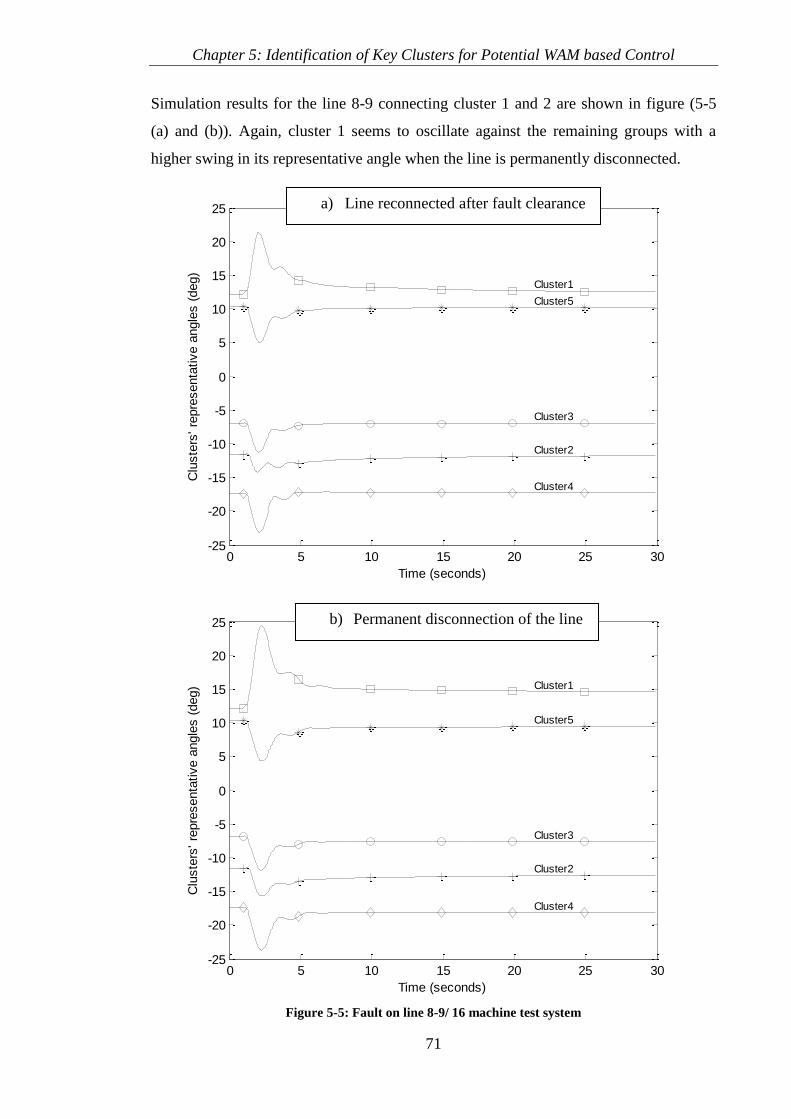
Chapter 5: Identification of Key Clusters for Potential WAM based Control
71
Simulation results for the line 8-9 connecting cluster 1 and 2 are shown in figure (5-5
(a) and (b)). Again, cluster 1 seems to oscillate against the remaining groups with a
higher swing in its representative angle when the line is permanently disconnected.
0 5 10 15 20 25 30-25
-20
-15
-10
-5
0
5
10
15
20
25
Cluster1
Cluster2
Cluster3
Cluster4
Cluster5
Time (seconds)
Clu
ste
rs' re
pre
senta
tive a
ngle
s (
deg)
0 5 10 15 20 25 30-25
-20
-15
-10
-5
0
5
10
15
20
25
Cluster1
Cluster2
Cluster3
Cluster4
Cluster5
Time (seconds)
Clu
ste
rs' re
pre
senta
tive a
ngle
s (
deg)
Figure 5-5: Fault on line 8-9/ 16 machine test system
a) Line reconnected after fault clearance
b) Permanent disconnection of the line

Chapter 5: Identification of Key Clusters for Potential WAM based Control
72
Figures (5-6) and (5-7) show results for the set of lines connecting the coherent clusters
2 and 5 (line 46-49 and line 50-51 respectively).
0 5 10 15 20 25 30-20
-15
-10
-5
0
5
10
15
Cluster1
Cluster2
Cluster3
Cluster4
Cluster5
Time (seconds)
Clu
ste
rs' re
pre
senta
tive a
ngle
s (
deg)
0 5 10 15 20 25 30-20
-15
-10
-5
0
5
10
15
20
Cluster1
Cluster2
Cluster3
Cluster4
Cluster5
Time (seconds)
Clu
ste
rs' re
pre
senta
tive a
ngle
s (
deg)
Figure 5-6: Fault on line 46-49/ 16 machine test system
a) Line reconnected after fault clearance
b) Permanent disconnection of the line

Chapter 5: Identification of Key Clusters for Potential WAM based Control
73
0 5 10 15 20 25 30-20
-15
-10
-5
0
5
10
15
Cluster1
Cluster2
Cluster3
Cluster4
Cluster5
Time (seconds)
Clu
ste
rs' re
pre
senta
tive a
ngle
s (
deg)
0 5 10 15 20 25 30-30
-20
-10
0
10
20
30
Cluster1
Cluster2
Cluster3
Cluster4
Cluster5
Time (seconds)
Clu
ste
rs' re
pre
senta
tive a
ngle
s (
deg)
Figure 5-7: Fault on line 50-51/ 16 machine test system
a) Line reconnected after fault clearance
b) Permanent disconnection of the line

Chapter 5: Identification of Key Clusters for Potential WAM based Control
74
Figure (5-6 (b)) however shows a different scenario as line 46-49 is permanently
disconnected to clear the fault. Clearly, cluster 5 encounters most of the impact as its
representative angle increases significantly. Figure (5-7 (b)) also shows that permanent
disconnection of the other line connecting cluster 2 and 5 (line 50-51) causes the
representative angle of cluster 5 to increase significantly away from the rest of the
system. It also shows that cluster 2 in the other end of the critical line under
consideration seems to oscillate against cluster 5 (keep in mind that these two clusters
are connected by the line under consideration).
Figure (5-8) and show the results with regard to line 41-42 connecting clusters 3 and 4
whereas figure (5-9) shows the results for line 42-52 connecting clusters 4 and 5.

Chapter 5: Identification of Key Clusters for Potential WAM based Control
75
0 5 10 15 20 25 30-20
-15
-10
-5
0
5
10
15
Cluster1
Cluster2
Cluster3
Cluster4
Cluster5
Time (seconds)
Clu
ste
rs' re
pre
senta
tive a
ngle
s (
deg)
0 5 10 15 20 25 30-25
-20
-15
-10
-5
0
5
10
15Cluster1
Cluster2
Cluster3
Cluster4
Cluster5
Time (seconds)
Clu
ste
rs' re
pre
senta
tive a
ngle
s (
deg)
Figure 5-8: Fault on line 41-42/ 16 machine test system
a) Line reconnected after fault clearance
b) Permanent disconnection of the line

Chapter 5: Identification of Key Clusters for Potential WAM based Control
76
0 5 10 15 20 25 30-20
-15
-10
-5
0
5
10
15
Cluster1
Cluster2
Cluster3
Cluster4
Cluster5
Time (seconds)
Clu
ste
rs' re
pre
senta
tive a
ngle
s (
deg)
0 5 10 15 20 25 30-25
-20
-15
-10
-5
0
5
10
15
Cluster1
Cluster2
Cluster3
Cluster4
Cluster5
Time (seconds)
Clu
ste
rs' re
pre
senta
tive a
ngle
s (
deg)
Figure 5-9: Fault on line 42-52/ 16 machine test system
a) Line reconnected after fault clearance
b) Permanent disconnection of the line

Chapter 5: Identification of Key Clusters for Potential WAM based Control
77
5.4. Summary
A method to evaluate critical areas and critical lines in multi-machine power systems is
discussed in this chapter. The method combines the concept of Centre of Inertia COI
and coherency property between synchronous generators to, firstly, identify coherent
clusters of synchronous generators within the power system and, secondly, to represent
each coherent cluster by its representative centre of angle (inertia). This allow for each
cluster to be evaluated with regard to the centre of angle of the entire system. Hence,
determine which clusters/lines are most critical for the system stability. The method is
tested on the standard 16-generator 68-bus system. The reason of choosing this
particular system is that is include 5 distinctive clusters and a number of tie-lines
connecting those clusters for which a number of scenario can be considered. The
obtained results are presented and discussed. The results show the effectiveness of the
proposed technique in giving a clearer sight regarding the system stability in terms of its
capability to illustrate the degree of criticality of certain areas and tie-lines connecting
these critical areas. The advantages of the proposed method can be summarised in the
following:
The method is based on coherent clusters identified based on coherency property
extracted from direct measurements2. Therefore, implementing the technique in
a wide-area measurement system is applicable; hence, critical areas/lines can be
identified directly without the need for the system model.
Identifying critical areas/lines allows better control schemes based on the
evolving technologies of wide-area measurement to be designed more
effectively. The critical lines, for example, where the system oscillations are
highly observable, can be taken as basis to provide wide-area feedback control
signals for local controller and power system stabilizers to enhance their
performance in damping system oscillations.
2 As described in chapter 4

Chapter 6: Development of a Novel WAM based Control Scheme for Stability
Enhancement
78
Chapter 6: Development of a Novel WAM based Control
Scheme for Stability Enhancement
6.1. Overview
A reliable, continuous supply of electricity is essential for today’s societies. Giving the
combination of increasing energy consumption and variety of reasons that limit the
extension of existing transmission networks, the situation requires less conservative
power system operation style. This can be possible only by monitoring and controlling
the system in a much more detailed and efficient way. In chapter 3, three different
control strategies are explored. The strategies are categorised in terms of the way
information are collected from the system and how control actions are taken and
deployed (i.e. centralised control, decentralised control, and multi-agent control
techniques). Another way of categorising control strategies is by looking at the level in
which control actions are taken. In electrical power systems, a three different control
levels can be identified [51]. Those control levels are:
Generating unit controls: This control level consists of system components that
apply their control actions directly to the generating unit. It consists of prime
mover control and excitation control with automatic voltage regulators (AVR)
and power system stabilisers (PSS). Prime movers control the generator speed
deviation and energy supply system variables. On the other hand, excitation
systems maintain the generator terminal voltage and reactive power flow within
acceptable limits.
System generation control: This control level aim is to determine active power
output such that the overall generation is equal to the system demand. It also
maintains the system frequency and controls the power flow across tie-lines
between different areas within the power system.

Chapter 6: Development of a Novel WAM based Control Scheme for Stability
Enhancement
79
Transmission control: This control level consists of system components that
monitor and control voltage levels and power flows across the transmission
system such as tap-changing transformers, synchronous condensers and static
VAR compensators.
In real system operation, these control levels are interlocked. All control actions affect
both components and system. AVRs for example are known to introduce oscillatory
modes, both local and inter-area, which are counteracted by deploying power system
stabilizers PSS. Generating unit control is a complete closed-loop system. A
considerable effort has been delegated to improve the performance of the controllers.
Some of these attempts are reviewed in chapter 3. The main problem, however, is that
the control law is derived based on a linearized system model in which the control
parameters are tuned to some nominal operating conditions. In the case of large
disturbances or power oscillations, the system state changes in a highly non-linear
manner and, in some cases, controllers become ineffective. In addition, generating unit
control level is considered as decentralised form of control strategies which consists
mainly of local controllers that lack the ability to have a wide view of the entire system.
Thus, their control actions are taken based on locally available control signals, which
limit their capabilities to influence and enhance the stability of the entire system.
This chapter is focused on the phenomenon of power system oscillation and the
development of a new control scheme to improve stabilisation capabilities of generating
units’ control. This will be carried out by means of adaptive control techniques and
exploiting the advantages of wide-area measurement systems WAMS.
6.2. Excitation Control and Stabilisation (advantages and limitations)
In power systems, the main components used to produce electrical energy are the
synchronous generators. The generator is normally driven by a prime mover and its
production windings are connected to the transmission network through a step-up power
transformer. Auxiliary circuits are used to control and manage the generator when
connected to the grid. Figure (6-1) shows a typical complete generating unit with most
auxiliary components [52]. The excitation system supplies the DC rotor windings with a

Chapter 6: Development of a Novel WAM based Control Scheme for Stability
Enhancement
80
field current (If) which, in turns, produces a rotating magnetic field that induces an
electromotive force (emf) in the generator stator windings. The excitation voltage (Ef) is
applied to the rotor windings and is controlled by an automatic voltage regulator (AVR).
During normal steady-state operation, the AVR is very effective in keeping satisfied
operation conditions. However, following a system disturbance, the system state
changes significantly in a non-linear manner and the AVR may have a negative impact
on the damping of power oscillations.
In presence of power swings, electric currents, which are proportional to the speed
deviation (∆ω) around the synchronous speed, are induced in the damper windings of
the synchronous generator. These currents result in a natural damping of the rotor
oscillations.
Synchronous
Generator
Measuring
elements
ExciterAutomatic Voltage
Regulator (AVR)
Speed
Governor
Prime Mover
(Turbine)
Step-up power
transformer
Unit
transformer
High voltage
network
Auxiliary
services
Pref
P
f
w
V
I
Vref
Va
lve
s
Shaft
Field current, If+ -
Generator terminals
Working fluid in
Working fluid out
Figure 6-1: Typical generating unit with most auxiliary components [52]
Chapter 6: Development of a Novel WAM based Control Scheme for Stability
Enhancement
81
As power swings cause the generator terminal voltage to oscillate, the reaction of the
AVR forces field current changes to maintain the voltage. Under certain conditions,
these field current changes may oppose the natural damping currents induced by the
rotor speed deviations ∆ω. In such cases, the AVR actions result in an artificial damping
that is large, negative and may be stronger than the natural damping. This phenomenon
is known as negative damping. Negative damping causes oscillatory unstable behaviour
in the system which needs to be stabilised. Power oscillations are unacceptable state of
operation that needs to be dealt with effectively and any power swings have to be
quickly damped. Thus, techniques to improve the performance of excitation systems in
such a way that they do not introduce negative damping or, even better, that they
introduce positive damping are important for more efficient, secure and reliable system
operation.
One way of improving excitation systems performance is using power system stabilisers
PSSs. The use of PSS is the most cost-effective and widespread method of enhancing
the damping of power oscillations. The function of a PSS is to reduce the negative
damping caused by AVRs actions by introducing a supplementary additional control
signal that compensate for voltage oscillations and provides a damping component that
is in phase with the speed deviation. Nonetheless, there are problems associated with
designing a robust and an effective PSS which results on it being unable to provide
satisfactory performance that can cope with the recent challenges facing modern today’s
power systems. Those problems or limitations are summarised as follows:
A typical PSS produces its control actions based on a defined transfer function
with constant parameters. In most cases, this transfer function consists of a
washout blocks and one or more phase compensation blocks as shown in figure
(6-2), [53]. Washout blocks are high-pass filters used to allow signals
associated with the speed deviations to pass unchanged and to reduce the
response of the damping during sever events. Phase compensation blocks are
used to provide the required lead/lag characteristic to compensate for the phase
shift caused by the exciter action, hence, overcome the negative damping
caused by those actions. Having constant parameters means that during rabid

Chapter 6: Development of a Novel WAM based Control Scheme for Stability
Enhancement
82
changes in system conditions, the PSS control action may not be able to
provide appropriate control signals which may cause system instability.
RsT1
1
w
w
sT
sT
1 2
1
1
1
sT
sT
4
3
1
1
sT
sT
pssK
pssVInput
Transducer washout Phase compensationLimiter
Figure 6-2: Block diagram of conventional PSS [53]
Most conventional PSSs are designed using linearized system models. Using
approximate linearized model of the generator and the power system, the PSSs
are designed using linear control theory. Although this design approach may be
effective during certain operation conditions, linearly designed PSSs may not
be able to maintain adequate stable operation conditions when power systems
are subjected to large disturbances that cause considerable and rabid changes in
system conditions.
Conventional PSSs use phase compensation blocks shown in figure (6-2) to
provide an electrical torque, which is in phase with speed deviation, to
compensate for the negative damping caused by actions of AVRs. The problem
with this design approach is that these blocks usually provide efficient
compensation only for a certain range of oscillation frequencies. As explained
in chapter 3, the frequency range of oscillations varies considerably between
local oscillation modes and inter-area oscillation modes. Therefore, it becomes
very difficult to design a PSS that is properly tuned to be as effective for
damping inter-area oscillations as it is in the case for local oscillations
damping.
Another important aspect of conventional PSSs is that they are decentralised
local controllers that act upon locally measured feedback control signals. PSSs
control based on local measurements are not always effective due to lack of
global observability, mutual coordination with other individual controllers, and
placement flexibility. Lack of global view of power system and absence of
Chapter 6: Development of a Novel WAM based Control Scheme for Stability
Enhancement
83
coordination between decentralised stabilisers may result in potentially harmful
interactions between these controllers.
Obviously, to meet today’s power systems operation requirements, development of
control schemes to enhance the performance of existing conventional controllers is
essential. Using global signals fetched from different parts of the network and applying
these signals as inputs to newly developed controllers can overcome the issue of
observability and lack of information of local controllers. Hence, enhance their damping
capabilities to instability phenomenon cause by power oscillations. With the advent of
new technologies of PMU/WAM based systems, it becomes possible to transmit wide-
area synchronised dynamic information across the entire system and make this
information available for local decentralised controllers. Also, using different control
design approaches alternative to linear control design theory can help overcome the
limitations inherited in such linearly designed controllers. Adaptive and artificial
intelligent control design approach to develop stability enhancement schemes provide a
promising way of making power systems more flexible, more adaptable to changes in
the system, and overall, more capable of providing a reliable and secure source of
electrical energy supply. The following sections of this thesis are focused on adaptive
non-linear control approach and its application in the power system; this is Fuzzy Logic
Control (FLC) design techniques and its application in power system.
6.3. Fuzzy Logic and its Application to Power Systems
Fuzzy logic theory has achieved considerable success in a variety of engineering
practices ranging from simple small applications to sophisticated decision making and
control problems. In [54], a relatively recent survey lists nearly 300 archival
publications related to fuzzy logic theory and its applications in power systems. It
provides a comprehensive set of references classified according to the power system
area, mainly published in archival journals on the fuzzy set theory applications in power
systems in the period from 1994 to 2001. In the area of power system operation and
control, traditional analytical solution techniques exist to deal with power system
problems. Although a considerable number of assumptions and approximations are
made to achieve these mathematical formulations, the solution for a large-scale

Chapter 6: Development of a Novel WAM based Control Scheme for Stability
Enhancement
84
interconnected modern power system problem is not always simple and adequate to deal
with ever changing system conditions. In addition, electrical power systems are large,
complex extended electro-mechanical dynamic systems that are geographically widely
spread and are influenced by unexpected events and continuous change of system
operating conditions. In such systems, many uncertainties exist within the operation due
to a large number of causes. These aspects makes it very challenging to effectively
operate and control power systems in today’s environment by relying solely on strict
conservative mathematically formulated solutions. Therefore, adopting alternative
theories, such as fuzzy set theory-based approach, can provide a complementary tool to
mathematical approaches for solving power system problems. In comparison to
traditional logic which uses variables that have precise values called “crisp” values,
fuzzy logic assigns a “set” of values to the variables to account for imprecisions and
uncertainties. Each value has a degree of membership of the set which represent the
probability of the variable having that value. A membership function identifies the
degree of membership over the range of possible values, known as the universe of
discourse. This function can be defined to represent an adjective, known as a linguistic
variables or fuzzy set, which describes the set of variables. The linguistic variables are
variables whose values are words rather than numbers. This ability of using common
linguistic terminology, that is easy to understand, allows fuzzy logic to model
qualitative reasoning and to be used in knowledge representation. The advantages of
using fuzzy logic or fuzzy set theory over conventional problem solving techniques can
be summarised as follows [55], [56], [54] and [57] :
Fuzzy logic uses natural language terms used by experts which are conceptually
easy to understand.
It is tolerant to imprecise data and can handle ambiguity.
It can be built on top of the experience of experts, (i.e. it allows for
incorporating the human experience in the design process).
It can resolve conflicting objectives by designing weights appropriate to the
selected objectives.
It is flexible and relatively easy to implement.
It can provide a smooth mapping between input and output data.
Fuzzy rules can be tuned either on- or off-line.

Chapter 6: Development of a Novel WAM based Control Scheme for Stability
Enhancement
85
Fuzzy logic is capable of modelling nonlinear functions of arbitrary complexity.
This makes it an appropriate alternative to linear theory of control design.
Fuzzy logic does not necessarily replace conventional control methods; rather it
can be blended with conventional control techniques. In fact it augments them,
simplify their implementation and enhance their performance.
The fact that the basis of fuzzy logic theory is the basis of human communication
underpins many of the other advantages of fuzzy logic. Because fuzzy logic is built on
the structure of qualitative description used in everyday language, it is therefore easy to
use, easy to implement and easy to tune. Also because experience and knowledge of
experts are very important in power system operations, fuzzy logic is ideal and can be
very effective for representing uncertainties and imprecisions in systems data by
fuzzification of ambiguous variables and assigning membership functions based on
preferences and experiences. It also remains possible to alter and adjust the fuzzy
system’s way of performance whenever new aspects are learned about the behaviour of
the power systems which makes such systems adaptable and flexible.
6.3.1. Application of Fuzzy Logic in Power Systems
In recent years, fuzzy logic applications have received increasing attention in many
areas of power systems. The objectives of these applications concentrate on the
applicability of fuzzy logic to power systems for wider operating conditions and
uncertainties. In the available literature, a number of distinctive areas in which fuzzy
logic is been applied to demonstrate the advantages of fuzzy systems over conventional
systems. These application areas can be classified based on the objectives of the fuzzy
system as follows:
A. Control
Fuzzy logic control (FLC) is an area for which fuzzy set theory is used to model control
decisions. In comparison with a conventional controller where the system is modelled
analytically using a set of differential equations from which the control parameters are
configured to satisfy the controller objective function, fuzzy logic-based controllers

Chapter 6: Development of a Novel WAM based Control Scheme for Stability
Enhancement
86
adjust the control parameters using a fuzzy rule-based expert system. For a fuzzy logic
controller, choosing the appropriate variables as input and output signals for the
controller is a critical task. Once input and output variables are chosen, it is required to
decide on the linguistic variables which are used to transform the numerical crisp values
of the input of the fuzzy controller to fuzzy quantities. The number of these linguistic
variables influences the quality of the performance of the controller significantly. As the
number increases, the computational time and memory requirements increases and, as
always, a compromise has to be made to choose the number of linguistic variables. The
use of fuzzy logic in the area of power system control is apparent in a number of
applications such as [54], [58]:
1. Fuzzy logic-based power system stabilisers.
2. Automatic generation control (AGC)/ load frequency control (LFC).
3. FACTS devices control.
4. Reactive power/Voltage control.
As any form of control category, fuzzy system applications in the area of power system
control aim to provide and satisfy a number of objectives. The objectives of fuzzy logic
control FLC in power system can be summarised in the following [56]:
1. To improve the control task performance and make it adaptable, flexible and
more robust.
2. To provide a way of expression of non-linearities and uncertainties in power
systems.
3. To allow for expert and operators experience to be implemented since heuristic
and expert knowledge are essential in power system operation and control.
4. To improve cooperation between various controllers and allow for multi-
objective coordination.
B. Planning, Operation and Optimisation
The issues associated with power systems planning and operation tasks are decision
making and optimisation problems. It is a fact that power systems are large
interconnected systems which are generally spread over wide geographic areas. Giving
the circumstances in which such complex systems operate including deregulation,

Chapter 6: Development of a Novel WAM based Control Scheme for Stability
Enhancement
87
privatisation, and the competitive market environment, minimising cost of operation
while maintaining high standard of security, reliability and quality of supply are
important and critical tasks that need to be satisfied. In tasks where minimising costs
and increasing system reliability form the main objectives, uncertainties arise and
system constraints are not always well-defined. An example to this is the optimal power
flow problem where constraints include generator and load bus voltage levels, line flow
limits, and reserve margins. Such constraints are ambiguous and the objectives are not
well-defined. In such cases, fuzzy set theory can provide a better solution to that
provided by traditional approaches. The use of fuzzy logic theory in the area of power
system planning, operation and optimisation can be seen in some applications including
[54], [58]:
1. Optimal power flow.
2. Generator maintenance scheduling.
3. Unit commitment.
4. Load forecasting.
5. Power system stability analysis (contingency analysis).
6. Voltage security analysis (reactive power/voltage control).
7. State estimation.
8. Security assessment.
9. Power system reliability evaluation.
10. Economic dispatch.
The objectives of the application of fuzzy set theory in the areas of power system
planning and operation where decision making and optimisation related problem make
up the main issues can be summarised as follows [54], [56]:
1. To achieve flexible and robust planning.
2. To provide a way of expression of uncertainties in power system.
3. To provide a way of expression of probabilities (such as in the case of
contingency analysis and stability evaluation).
4. To improve accuracy as in load forecasting.
5. To reduce computation time.
6. To provide an expression of experience based rules.

Chapter 6: Development of a Novel WAM based Control Scheme for Stability
Enhancement
88
C. Protection and Diagnosis
Reliable operation of power systems relies primarily on properly functioning and
maintained equipment. Preventing equipment failure from damage caused by faults and
disturbances in the system depends on designed protective and relaying schemes. In
protection systems, various relaying signals such as currents, voltages and line
parameters are determined with a degree of approximation. This approximation results
in inaccuracy which can prove costly during sever faults in the system. Also fault
diagnosis can be a difficult task during multiple faults and relaying equipment failure.
Failure of protective relays or circuit breakers results in uncertainties and inaccuracy of
decision-making process. In such cases fuzzy logic can be suitable to deal with these
uncertainties and be very effective in enhancing the accuracy of protection schemes
[54].
In conclusion, fuzzy logic theory can handle approximate information and system
uncertainties in a systematic way. Therefore, it is ideal for dealing with system
nonlinearity and modelling complexity where inexact model exists or where ambiguity
is common. As for power systems, fuzzy logic can provide an appropriate alternative
technique to develop solutions to various problems related to control and operation of
these systems. In the following section, the focus is put on utilizing fuzzy set theory in
the area of power system control. A particular are of interest is using fuzzy logic theory
to develop stability control scheme to enhance system stability and allow for better
system utilization.
6.3.2. Fuzzy Logic based Power System Stabilisers FPSS
Power system stabilisers PSSs are the most cost-effective and widespread method of
enhancing power system oscillation damping and improving overall system stability.
Conventional power system stabilisers (CPSSs) have been implemented on actual power
systems for this purpose and have provided significant enhancement for the overall
stability of power systems [17], [59]. However, as indicated previously (section 6.2),
there is a number of limitations to these CPSSs such as their fixed parameters which are
tuned to ensure optimal controller performance at a nominal operating point.

Chapter 6: Development of a Novel WAM based Control Scheme for Stability
Enhancement
89
Consequently, CPSSs performance could degrade whenever their operating point is
shifted from nominal. In order to overcome the disadvantages of the widely used
CPSSs, alternative design techniques have, recently, received a considerable attention.
As a result, fuzzy logic has emerged as a powerful tool in designing fuzzy logic based
power system stabilisers (FPSSs). The reasons are that the application of fuzzy logic
control (FLC) techniques seems to be most suitable in such circumstances when a well-
defined control objective cannot be specified and the involved system is very complex
or its exact mathematical model is not available. Fuzzy logic approach to control design
is simple, better alternative to nonlinear control techniques, easy to understand, robust
and have relatively low computation requirements. They also can be built on top of
conventional controller to enhance the overall control performance.
Attempts to use fuzzy logic techniques to develop power system stabilisers are well-
documented in the literature. In [60] and [61] the basic configurations of a fuzzy logic
controller FLC is described. In comparison to the configurations of conventional
control, in which the control process is expressed through a set of mathematical
equations that determines the relation between specified numbers of data inputs, fuzzy
logic control FLC design approach resembles that of a knowledge-based technique.
Fuzzy logic controllers are basically rule-based controllers that utilise the principle of
fuzzy set theory in its data representation and its logic. A typical structure of an FLC is
shown in figure (6-3) [60]. The basic configuration of an FLC can be simply presented
in four main parts. Those are input and output scaling factors, fuzzifier, de-fuzzifier,
rule-base and fuzzy inference engine.
Figure 6-3: Basic configuration of Fuzzy Logic Controllers (FLC) [60]

Chapter 6: Development of a Novel WAM based Control Scheme for Stability
Enhancement
90
A. Fuzzification
The fuzzification is a process by which the crisp input control variables are transformed
into fuzzy linguistic variables using normalized membership function [62].
B. Knowledge-base and Inference Engine
The fuzzy logic inference engine is the part responsible for deducing the proper control
action based on the available rule base. The knowledge base includes the definition of
the fuzzy membership functions, defined for each control variable, and the required
rules that determine the control action using linguistic variables. It enables the controller
to map the input fuzzy sets to the output fuzzy sets through control rules in the form of
IF-THEN statements. This part of the control design allows for incorporating the human
experience in the design process as some of these rules can be derived based on past
experience, knowledge acquired through off-line simulation, understanding of the
dynamics of the involved system and common sense engineering judgment [63].
C. De-fuzzification
The de-fuzzification is a process by which the fuzzy linguistic output control action is
transformed into proper crisp values using normalized membership function [62].
D. Input and Output Scaling Factors
The input and output scaling factors are important in order to allow for a wide range of
operating conditions to be considered without having to consider the physical domain of
the input and output signals [64]. As recommended in [65], the range of the membership
function for all input and output signals should be kept between ± 1. Input scaling
factors are therefore required to normalise the inputs magnitudes so that they are
contained in the chosen range. Similarly, output scaling factor is required to de-
normalize the output signal.
Chapter 6: Development of a Novel WAM based Control Scheme for Stability
Enhancement
91
6.3.2.1. Design Procedure of Fuzzy Power System Stabilizer FPSS
Figure (6.3) shows the main components of a fuzzy logic based controller. However, for
fuzzy logic based power system stabilisers FPSSs, the design process can be split into a
number of steps as described below [60].
A. Selection of Control Variables (Input and Output Signals)
To design a fuzzy logic controller FLC, variables that describe the dynamic behaviour
of the subject to be controlled should be chosen as input signals to the controller. It is a
common practice to use the output error (e) and the rate of change or the derivative of
the output (ė) as control inputs [60]. The input and output variables for an FPSS can be
described as in equation (6.1).
pssj ueeX ,, (6.1)
In many cases of FPSS design, the generator speed deviation (∆ω) and its derivative
(∆ώ), which resembles the acceleration, are considered as inputs for the controller [66],
[67], [68],[69], [70] and [71]. In other applications, the speed deviation (∆ω) and the
active power deviation (∆Pe) of the synchronous generator are chosen as input signals to
the controller [61], [72], [73], [74], [75]. In both cases, normally two appropriate scaling
factors are applied to the speed deviation and acceleration/active power deviation and
then both control signals are fed to the FPSS. The output signal of the controller (upss) is
also scaled using an output scaling factor and added to the AVR as a supplementary
control signal.
B. Membership Function Definition
The measured crisp input variables are converted into fuzzy variables. The universe of
discourse (i.e. the set that contains the entities over which certain variables may range
[76]) of each fuzzy variable can then be quantised into a number of overlapping fuzzy
sets known as linguistic variables. In practical applications, the universe of discourse is
restricted to a small range (Xmin , Xmax) [60]. The number of the linguistic variables

Chapter 6: Development of a Novel WAM based Control Scheme for Stability
Enhancement
92
varies according the control application. Normally odd numbers are used (3, 5, 7 …).
Higher number of linguistic variables results in an increase in the number of the rules
required to fire the appropriate control action. In most FPSS applications, seven
linguistic variables are chosen to represent the crisp input values by fuzzy sets. Those
seven linguistic variables used to represent each input and output signals are (NB)
negative big, (NM) negative medium, (NS) negative small, (Z) zero, (PS) positive small,
(PM) positive medium and (PB) positive big. A membership function that maps the
crisp values into fuzzy values is assigned to each fuzzy linguistic variable. A
membership function can differ in shapes (i.e. triangular, trapezoidal, or a bell shape).
For the application of FPSS, the most commonly used shape is the triangular shape
shown in figure (6-4) [60].
Figure 6-4: Triangular membership functions for FPSS input and output variables [60]
A triangular membership function of this configuration shown in figure (6-4) can be
expressed by equation (6.2).
iii
i
ii
iii
i
ii
i
xforx
xforx
xF
)( (6.2)
Where µi is the centroid of the ith
membership function and σi is a constant which
identifies the spread of the ith
membership function [60].
NB NM NS Z PS PM PB
-L L0
1
Xmin
Xmax
Xrange
2
i

Chapter 6: Development of a Novel WAM based Control Scheme for Stability
Enhancement
93
For simplicity, the membership functions are assumed to be symmetrical and each one
overlaps its adjacent function by 50% as shown in figure (6-4). By using membership
functions of this type, the input variables can then be transferred into linguistic fuzzy
variables. For practicality, the membership functions need to be normalized in the
interval [-L, L], which is symmetrical around zero. For this particular reason, the control
signal amplitudes are expressed in terms of controller parameters known as the scaling
factors (gains) as shown in figure (6-3). The input and output scaling factors are
important in order to allow for a wide range of operating conditions to be considered
without having to consider the physical domain of the input and output signals. The
scaling factors or the controller parameters can be defined as in equation (6.3) [60],
[51].
jrange
jX
LK
2 (6.3)
Where Kj is the input and output scaling factors and are referred to as the fuzzy logic
controller parameters, jrangeX is the full range of the control variable Xj, which from
figure (6.4), can be described as in equation (6.4).
jjjXXX range minmax (6.4)
Wherej
X max , j
X min are the maximum and the minimum values of the control variable
Xj.
The parameters of the membership function (σi, µi) can be identified using the above
definitions using equations (6.5) and (6.6).
1
n
Xjrange
i (6.5)
ii KXj
1min (6.6)
Where i= 1,…….,n and n is the number of linguistic variables

Chapter 6: Development of a Novel WAM based Control Scheme for Stability
Enhancement
94
C. Rule-base and Inference
The basics of fuzzy logic systems relies on a process of mapping an input fuzzy set to
an output fuzzy set which forms the control action. This is acquired by a set of fuzzy
rules which determines the relation between those fuzzy sets. The knowledge base and
the inference engine shown in figure (6-3) are the parts responsible for this mapping
process. The proper control action is deduced based on the available rule-base. The
knowledge-base includes the definition of the fuzzy membership function defined for
each control variable and the required rule that determines the control action using
linguistic variables. This process of mapping the input fuzzy sets to the output fuzzy
sets is achieved through control rules in the form of IF THEN statements. This part of
the control design allows for incorporating the human experience in the design process
as some of these rules can be derived based on past experience, knowledge acquired
through off-line simulation, understanding of the dynamics of the involved system and
common sense engineering judgment. For the design of fuzzy logic based power system
stabilizers, techniques to derive and optimise the required rule-base are well-
documented in [60] and [65]. The required number of rules depends on the number of
the linguistic variables being assigned to each input variable. As indicated above, most
FPSS applications use seven linguistic variables to represent the crisp input values by
fuzzy sets (NB, NM, NS, Z, PS, PM, and PB). As a result, 49 (7×7) control rules are
required to relate those control variables to each other. Table (6.1) provides a generic
control rules for fuzzy controllers used as power system stabilisers [60].
Table 6-1: Decision table of fuzzy control rules for an FPSS
Speed
deviation
(∆ω)
Derivative of speed deviation (∆ώ) / active power deviation (∆Pe)
NB NM NS Z PS PM PB
NB NB NB NB NB NM NS Z
NM NB NB NM NM NS Z PS
NS NB NM NM NS Z PS PM
Z NM NM NS Z PS PM PM
PS NM NS Z PS PM PM PB
PM NS Z PS PM PM PB PB
PB Z PS PM PB PB PB PB

Chapter 6: Development of a Novel WAM based Control Scheme for Stability
Enhancement
95
The inference mechanism utilises the above table to determine the fuzzy set of the
control action using IF THEN statements in the form “if A, then B,” where A is the rule
antecedent and B is the rule consequence. Every entity in table (6.1) represents a rule.
The antecedent of each rule conjoins the two fuzzy input variables. The first input
variable is the speed deviation (∆ω) which represent the error (e) described by equation
(6.1). The second input variable can be either the derivative of the speed deviation (∆ώ)
or the active power deviation (∆Pe) which represent the derivative of the error (ė) shown
in equation (6.1). An example to a randomly picked ith
rule is as in:
If ∆ω is NB and ∆Pe is NM then upss is NB
Determination of the degree of membership of the output linguistic variable is done
using what is known as MIN-MAX inference or the Mamdani type inference [65]. For
clarity of explanation, figure (6-5) shows an example (adopted from [77]) for
fuzzification of two input variables using membership function similar to that described
in figure (6-4). In figure (6-5) bellow, the two input variables are the speed deviation
∆ω and the active power deviation ∆Pe signals. As shown, the crisp value of ∆ω is
mapped into the PS and PM regions of the triangular membership function
( )(),( PMPS ), and is assigned a degree of membership equal to 0.8 and 0.2
respectively. Similarly, the crisp value of ∆Pe is mapped into the NS and Z regions
( )(),( ZNSee PP ) and is assigned a degree of membership of 0.7 and 0.3 respectively.
Figure 6-5: Example of fuzzification using triangular membership function (adopted from [77])

Chapter 6: Development of a Novel WAM based Control Scheme for Stability
Enhancement
96
The rule-base shown in table (6.1) is used to firstly, determine the output decision as a
linguistic output variable, and secondly, to assign a degree of membership or weight to
the output linguistic variable. Applying table (6.1) to this example using the IF-THEN
statement maps the output logistic variable into four regions (Z, PS, PS, PM) as shown
below.
If ∆ω is PS and ∆Pe is NS then upss is Z
If ∆ω is PS and ∆Pe is Z then upss is PS
If ∆ω is PM and ∆Pe is NS then upss is PS
If ∆ω is PM and ∆Pe is Z then upss is PM
The degree of membership assigned for the output linguistic variable is then determined
using what is known as MIN-MAX inference (it utilises the minimum function for the
implication of the rule, while the combination of all rules is represented be the
maximum function). The degree of membership for each output linguistic variable is
given by the minimum of the degree of membership of the two input linguistic variables
determining that output linguistic variable. For example, consider the first rule, (If ∆ω is
PS and ∆Pe is NS then upss is Z), the membership of the output linguistic variable (Z) is
determined as in equation (6.7) [51].
)(),(min)( NSPSZePout (6.7)
Applying this technique, the degree of memberships for all outputs can be determined
as shown in table (6.2).
Table 6-2: Example of rules activation in a fuzzy system
∆ω
∆Pe
NB NM NS (0.7) Z (0.3) PS PM PB
NB NB NB NB NB NM NS Z
NM NB NB NM NM NS Z PS
NS NB NM NM NS Z PS PM
Z NM NM NS Z PS PM PM
PS (0.8) NM NS Z (0.7) PS (0.3) PM PM PB
PM (0.2) NS Z PS(0.2) PM(0.2) PM PB PB
PB Z PS PM PB PB PB PB

Chapter 6: Development of a Novel WAM based Control Scheme for Stability
Enhancement
97
The output of the inference process at this stage is a fuzzy set. Once the memberships of
all output linguistic variables are assigned, a crisp discrete output is derived based on
de-fuzzification techniques which form the last step of the design procedure.
D. De-fuzzification strategy
De-fuzzification is the process by which a fuzzy controller produces its desirable crisp
numerical output from a fuzzy set of linguistic variables. As in the example above, if
two or more degrees of memberships are assigned to the same linguistic variable (i.e.
PM is assigned both 0.2 and 0.3) then the maximum of the weight is associated with the
linguistic variables (hence, MIN-MAX inference). By using these linguistic variables and
membership functions, an area can be formed as shown in figure (6-6). The centre of
gravity (also known as the centroid method) of the mapped area is then used to infer the
crisp output value. The centre of gravity method can be described by the following
equation [51].
Rules
i
i
out
Rules
i
i
outout
pss
Z
ZZu
u
1
1
)(
)()(
(6.8)
Where upss is the controller crisp output value, and )(Zi
out denotes the output
membership degree for the ith
rule associated with the output subset of Z, uout(Z).
Figure 6-6: Example of de-fuzzification of output signals (adopted from [77])

Chapter 6: Development of a Novel WAM based Control Scheme for Stability
Enhancement
98
In other words, the centre of gravity method is used to compute the centre of the area
encompassed by the fired rules in the knowledge base part of the controller which
results in a single crisp value that represent the controller output signal.
6.3.2.2. Enhancement of FPSS Performance
The feasibility of fuzzy logic based power system stabilizers FPSSs as stability
enhancement schemes has been demonstrated in a considerable amount of research
article. Fuzzy logic based techniques has been suggested as a possible solution to
overcome the problems and drawbacks associated with conventional power system
stabilizers CPSSs, discussed earlier in section 6.2. Thereby using fuzzy logic
techniques, complex system mathematical models can be avoided while providing good
performance under different operating conditions. Fuzzy logic is proved to have the
features of simple concept, easy implementation and computational efficiency, all of
which are important aspects of overall enhanced system performance.
Most of the early attempts to implement fuzzy logic technique to design FPSSs are
focused on developing decentralised controllers local to the specific plant or generator.
In [78], a controller that uses two real-time measurements of generator speed deviation
(∆ω) and the acceleration or the derivative of the speed deviation (∆ώ) as input signals
is developed based on simple fuzzy set theory [60]. Since only local measurements are
required by the developed FPSS on each generating unit, the stabilizer is of a
decentralised output feedback form of control and is easy for practical implementation.
It is also intended for multi-machine power system and the results obtained showed a
good dynamic performance over a range of operating scenarios. Reference [79]
introduces an FPSS that uses speed deviation (∆ω) and power output deviations (∆Pe) of
the local machine as the input variables for the fuzzy logic controller. The developed
controller performs the function of a power system stabilizer and provides a
supplementary control signal to the excitation system of the generator. The proposed
FPSS is developed for a single machine and procedures in the development of its
structure and rule base and the tuning of its parameters is described. The proposed
tuning methodology is based on an off-line process that adjusts the controller
parameters based on specified performance characteristics for the controlled system.

Chapter 6: Development of a Novel WAM based Control Scheme for Stability
Enhancement
99
The test results showed robust performance and effectiveness under various operating
conditions and disturbances. A similar design approach is described in [61] where speed
deviation (∆ω) and accelerating power (∆P) are used as input signals to the controller.
The developed FPSS is tested in a multi-machine power system environment in which
the tuning of the FPSS parameters is automatically carried out off-line by using a tuning
software extension module to the multi-machine simulation package. The tuning
module hierarchically lies on top of the simulation package and uses a blind search
algorithm to locate optimum or near-optimum controller gains that minimise certain
system performance indices. The results obtained in [61] showed that the proposed
FPSS can effectively damp both modes of oscillations (local modes and inter-area
modes) in a multi-machine power system. The results also showed that the developed
FPSS can work cooperatively with conventional stabilizers CPSSs. Reference [61] also
emphasise the importance of the location of the PSS; it states that in order to provide
efficient damping for both local and inter-area modes of oscillations, PSS have to be
installed on generators which are the main cause of the two modes of oscillations. It
also concludes that the lack of on-line complicated mathematical computations makes
fuzzy logic based techniques more reliable for real-time applications where small
sampling time may be required. In [80] an augmented FPSS is proposed to enhance
power system stability. The introduced controller utilises the fuzzy logic based
stabilizer in the usual manner, similar to that in [78] described above in terms of input
control variables. In addition it uses a modification of the terminal voltage feedback
signal to the excitation system as a function of the accelerating power on the unit. The
non-linear action of the proposed augmented FPSS increases the power system stability
significantly while it is simple to implement. The test results showed that implementing
the augmented controller in both single machine system and multi-machine power
system results in an enhanced dynamic performance over a wide range of operating
conditions. Article [68] provides a systematic approach to fuzzy logic control by which
a design and analysis of an adaptive FPSS is demonstrated. The proposed systematic
tuning methodology is intended to overcome the difficulties and drawbacks of manual
tuning of control rules and membership functions adopted in previous design attempts.
It assumes that while the quantity of the control law may change, its quality remains.
Thus control rules and membership functions are designed once and then modified by
systematic scaling techniques for a particular system and range of operating conditions.

Chapter 6: Development of a Novel WAM based Control Scheme for Stability
Enhancement
100
The advantage of the proposed design approach is that the controller is insensitive to the
precise dynamics of the system which gives it a degree of adaptability over a wide range
of operating scenarios. The test results demonstrated the effectiveness of this design
approach in developing a robust FPSS that is capable of system stability enhancement.
In [67] a design procedure for an FPSS is presented. Speed deviations and its derivative
are chosen as the input signals to the controller. A new technique that uses a normalised
sum-squared deviation (NSSD) index is utilised to determine the FPSS parameters and
acquire a proper tuning. The proposed tuning methodology is an off-line process that
adjusts the controller parameters by minimising a NSSD index evaluated for rotor angle
of pre-identified critical machine. The determination of the critical machine to which
the FPSS is assigned is achieved using the well-known concept of participation factors
[20] which are computed from the right and left eigenvectors of the system state matrix
of the power system. By using Eigen structure analysis, the oscillatory rotor modes are
identified first. Secondly, by comparing the participation factors of the speed
component of all the machines in the poorly damped rotor mode, the machine with the
highest participation factor is identified as the critical machine. The simulation results
showed the effectiveness of the response of the designed FPSS to various disturbances
in a multi-machine power system environment. It is also seen from the results that the
FPSS can damp both local and inter-area modes of oscillations effectively as well as
having a wider stable region with comparison to CPSS. An interesting design technique
is introduced in [81] which proposes a fuzzy logic-based adaptive power system
stabiliser for a multi-machine power system. The proposed design approach
accommodates two linear conventional stabilizers and a fuzzy logic-based signal
synthesizer. The two linear stabilizers are designed based on the traditional frequency
domain method for extreme loading conditions which allow them to generate stabilizing
signals working best under these conditions. The fuzzy-based synthesizer then combines
the two individual signals in such a way that the signal fits the loading condition
optimally. The fuzzy controller is optimised using a least squares error criterion and is
tested for a single machine infinite-bus as well as for a multi-machine system. The
results showed that the proposed FPSS provides adequate and satisfactory damping for
low frequency oscillations under a wide range of operating conditions and can perform
better than conventional stabilizers. Reference [66] introduces a modified method for

Chapter 6: Development of a Novel WAM based Control Scheme for Stability
Enhancement
101
designing fuzzy logic based power system stabilizers to counter the small signal
oscillatory instability in power systems. The modified technique alternatively represents
the two states of the generator ∆ω (speed deviation) and ∆ώ (acceleration), which form
the stabilizer input signals, in polar form and generate the stabilizing signal based on the
magnitude and angle of those signals. The designed stabilizer is shown to be easier to
implement in a multi-machine system and quite effective in damping both local and
inter-area modes of oscillation. A variable structure adaptive fuzzy logic based power
system stabilizer (AFPSS) is proposed in [75]. The proposed controller is a fuzzy logic
based stabilizer that has the capability of adaptively tune its rule base on-line. The
proposed controller is initialized using the rule base of a standard FPSS to ensure an
acceptable performance during the learning stages. The rule base is then tuned on-line
so that the stabilizer can adapt to and cope with different operating conditions. The
alterations and changes in the fuzzy rule base are carried out using a variable structure
direct adaptive control algorithm to achieve the pre-defined control objectives. The use
of such adaptive algorithm has the advantages of, firstly achieving a good performance
in the training stage as it makes use of the initial standard rule base of FPSS, and
secondly providing a robust estimator since it depends on a variable structure technique.
The adaptive feature of the proposed controller results in an improved performance as it
significantly reduces the rule base size and maintains satisfactory operation. This is
confirmed by simulation results of a single machine and a multi-machine power system
showing the effectiveness of the proposed AFPSS in damping power system
oscillations. A systematic approach for the design of an FPSS is presented in [82] which
have the potential to shorten the tuning process of fuzzy rules and membership
functions. The proposed technique breaks the design process into two stages. In the first
stage a proportional derivative type PSS (PDPSS) is developed. In the second stage, this
PDPSS is transformed into fuzzy logic stabiliser FPSS. Because this approach is
systematic and straightforward, it provides an easy and reliable scheme to overcome the
drawbacks of other methods used to tune the fuzzy controller parameters and rule base
such as trial and error methods or the use of searching algorithms such as genetic
algorithms (GA), which can be time consuming. Simulation results on a multi-machine
power system showed the technique to be effective in designing robust FPSS that is
capable of providing adequate damping for power system oscillations

Chapter 6: Development of a Novel WAM based Control Scheme for Stability
Enhancement
102
R. Gupta in [83] discusses a study of fuzzy logic power system stabilizer (FPSS) for
stability enhancement of multi-machine power systems. The proposed stabilizer uses a
reduced rule base limited to 25 decision rules (5×5), which relates the input control
signals (speed deviations ∆ω and acceleration ∆ώ) to the deduced control action.
Instead of using the extended standard 49 decision rule table shown in table (6.1),
reference [83] uses less membership functions and therefore less rules to achieve the
controller objectives. Also different de-fuzzification methods were used to quantify the
fuzzy output signal. This is found to have reduced the computation requirements while
maintaining satisfactory performance. Test results in a small two-area four-machine
system were quite encouraging and satisfactory. In [70] the performance of a
hierarchical FPSS, which is tuned automatically as the operating conditions of power
systems change, is evaluated by applying it to a multi-machine power system. Similar to
other fuzzy logic based stabilizers the proposed FPSS uses the speed deviation (∆ω) and
its derivative (∆ώ) as input signals. A function of adaptability is introduced into the
design by means of two scaling parameters which have the ability to adjust their values
as system conditions change. These scaling parameters are the output of another fuzzy
logic system (FLS), which acquire its inputs from the operating conditions of the power
system. In order to tune the FPSS, the two scaling factors are used to adjust the range of
inputs as operating conditions change (input signal 1= Kp ∆ω and input signal 2= Kd
∆ώ). The FPSS is tuned by computing optimum input scaling factors (Kp) and (Kd)
using another FLS that uses the electrical active power (Pe) and reactive power (Q) of
each machine as input signals to represent the operating conditions of each machine.
The FLS with two inputs (Pe and Q) is referred to as the tuner and the proposed scheme
is referred to as the self-tuning fuzzy logic power system stabilizer (TFPSS). This
process of tuning the FPSS makes it adaptive to changes in the system operating
conditions and allows for an enhanced overall system performance. Simulation results
showed that by using the proposed mechanism to tune the TFPSS on-line, better
response of the system can be achieved in a wide range of operating conditions
compared to fixed parameter FPSS and conventional CPSS, with the latter still the less
efficient of all. In [69] an alternative new approach for designing FPSS that utilises a
genetic and evolutionary algorithm (GEA) to optimise the scaling factors of the
controller is proposed. In this design approach the scaling factors or the controller
parameters are referred to as the normalisation and de-normalisation factors and the

Chapter 6: Development of a Novel WAM based Control Scheme for Stability
Enhancement
103
study is carried out considering an FPSS based on 3, 5 and 7 membership functions
(MFs) of Gaussian shape. The objective of the proposed design is to obtain an FPSS
which improves both transient and small signal stabilities of power systems and
investigate the effect of variation of a number of linguistic variables (membership
functions) on the performance of FPSS in order to obtain an optimum FPSS design with
a minimum number of MFs without jeopardizing the dynamic performance of the
system. The proposed design technique uses a conventional PSS to examine the
dynamic response of the system under study for different operating conditions and
obtain the maximum values of the input signals ∆ω and ∆ώ. Based on these
observations, initial values for the input scaling factors (normalisation factors) are set.
These values are considered as upper bounds of the input scaling factors (K∆ω and K∆ώ)
for further optimisation of these values using GEA. The upper bound of the output
scaling factor (de-normalisation factor) is set initially to equal 1. Once those values are
chosen, an algorithm for optimising the normalisation and de-normalisation factor using
GEA is used to optimise them. Simulation results of the proposed design showed a
robust performance of the FPSS for various operating conditions including small and
large disturbances. It also indicates that there is no merit in increasing the number of
MFs beyond 5.
A simplified fuzzy logic controller (SFLC) with a significantly reduced set of fuzzy
rules, small number of tuning parameters and simple control algorithm and structure is
described in [84]. The technique takes advantage of the symmetrical form of the rule
base commonly used in fuzzy control applications, as that shown in table (6.1).
According to [84], it is observed that, in the two-dimensional phase-plane, the required
control action magnitude deduced from the rule base is the same for both negative and
positive stabilising conditions and is proportional to the distance from the state of the
system to the switching line (defined by the desired zero consequence). Based on this a
simplified version of rule base is derived and a simplified fuzzy controller (SFLC) with
the same performance but reduced rule base is proposed. Based on the SLFC a
simplified power fuzzy logic power system stabiliser (SFLPSS) is designed and applied
to a single machine-infinite bus system. The performance of the proposed SFLPSS is
analysed over various load levels of the generating unit and different type of
disturbances. Simulation results showed that a SFLPSS with only four rules can provide

Chapter 6: Development of a Novel WAM based Control Scheme for Stability
Enhancement
104
the same response as a standard FPSS with the original and complete rule base. Also
compared with a CPSS, the proposed stabiliser showed an improved response and
effectiveness in damping power system oscillations, although, it has not been tested on a
multi-machine power system. An improved version of the self-tuned fuzzy logic power
system stabilizer (STFLPSS), which follows the same design approach as the previously
described one, is studied in [85] and is implemented in a computer simulations of a
multi-machine power system. In addition to the advantages of the SFLPSS described in
[84] (i.e. significantly reduced and one-dimensional rule table, small number of tuning
parameters, simple control algorithm and simple architecture and control design), the
latter [85] is able to non-linearly change, on-line, the sensitivity of the controller to the
input signal which allows it to provide improved control performance over a wide range
of changeable operating conditions, as the simulation results illustrated. In another
attempt to introduce robustness and adaptability into the control design, T. Hussien in
[86], describes a robust adaptive fuzzy controller as a power system stabiliser (RFPSS)
used to damp inter-area modes of oscillations. The proposed approach uses a particle
swarm optimisation algorithm to tune the controller input and output gains such that the
sum square of the speed deviations is minimised. This introduces adaptation capabilities
into the controller and allows it to cope with a wide range of operating conditions. The
robustness of the design is assured by using fuzzy logic to compute the nominal values
of the system non-linearities. Based on these values, conventional feedback linearization
is modified to ensure robustness and acceptable performance. Simulation results of a
four-machine two-area test system illustrated the enhanced performance of the proposed
RFPSS compared with CPSS. A similar design approach is adopted in an earlier
research [87] to develop an indirect variable structure adaptive fuzzy logic controller as
a power system stabilizer (IDVSFPSS) used to damp inter-area modes of oscillation
following disturbances in power systems. The designed stabilizer uses the speed and the
speed deviation, obtained on-line and assumed to be measured from the output of the
plant, as input signals. The output of the fuzzy identifier is the estimate of the unknown
non-linearities of the model and is used as a feedback linearization framework to
provide the necessary damping requirement to the power system. The design approach
also uses practical swarm optimisation based algorithm to tune the controllers
parameters (gains) such that the sum of the squares of the speed deviations is
minimised. Item [88] inspects three types of fuzzy control algorithms in the case of a

Chapter 6: Development of a Novel WAM based Control Scheme for Stability
Enhancement
105
single machine connected to the network. It introduces two types of single-input/single-
output control scheme and a third two-input/single-output control scheme, all of which
are designed based on fuzzy logic techniques. The study shed lights on the importance
of choosing the input control signals and how that might influence the controller
performance. The results confirmed that considerable improvement of the system
stability is achieved when using two-input/single-output control scheme with
comparison to single-input/single-output control scheme. It also concluded that,
although the design of the proposed FPSS is simple and requires no mathematical model
of generator and power system, as would be the case for CPSS, the overall performance
of the system is enhanced over a wide range of operating conditions and in the presence
of different disturbances, small and large.
As described above, many attempts to design effective decentralised fuzzy logic based
power system stabilizers (FPSSs) are well-documented in the literature. Great deals of
these attempts were successful in developing control schemes that are sufficient and
feasible. Clearly the superiority of fuzzy logic as a design tool to deal with the non-
linearities in power systems when it comes to PSS design is shown. The performance of
fuzzy logic based power system stabilisers (FPSSs) as local damping controllers is
superior to that of conventional stabilisers (CPSSs) which are designed based on the
traditional linear design approach. Nonetheless, these decentralised controllers remain
local control schemes which act upon local control signals. Local control signals maybe
sufficient enough in observing local modes of instabilities that results from local
oscillations at the local plant. Wide area instabilities such as inter-area oscillation modes
can be very difficult to be observed effectively in local signals. As bulk power transfers
are being exchanged between interconnected areas in complex modern power systems,
the need to deal with the rapid increase of inter-area oscillations has become essential to
enhance power systems’ stability, security and reliability of supply to meet customers
demand. Regardless to the design technique used to develop local power system
stabilisers (LPSSs), they have inherited limitations in damping inter-area modes of
oscillations due to lack of information and observability to this phenomenon. Inter-area
modes of oscillations are not highly observable and controllable in local signals as in
the case of local modes of oscillations [89], [63]. Due to this lack of system wide view
for LPSSs, their performance may not be as strong and reliable to damp inter-area

Chapter 6: Development of a Novel WAM based Control Scheme for Stability
Enhancement
106
modes of oscillations especially during sever disturbances. To ensure small signal
stability [6] of power systems, increasing interest has been focused on developing wide-
area based power system stabilisers (sometimes referred to as supervisory power system
stabilisers (SPSSs) [31], [89]) by means of remote feedback control signals to wide-area
based designed controllers. The advance technology in phasor measurement units PMUs
has facilitated this and has allowed for increasing attempts in developing global
controllers using wide-area measurement systems WAMS.
In section 3.2, some of these attempts are described based on the control strategy used
to develop the control scheme. In the following section, a novel design for a wide-area
based fuzzy logic power system stabiliser is introduced. The architecture and the basic
design of the proposed wide-area based stabiliser are described. The performance of the
proposed scheme is then tested by implementing it in a number of study cases through
computer simulations. The scheme is referred to as Global Fuzzy logic based Power
System Stabiliser (GFPSS). The use of fuzzy logic as a tool to design the proposed
controller is justified by the proved abilities and capabilities of fuzzy logic in providing
very good and efficient stability enhancement schemes, as discussed previously in this
chapter.
6.4. A Novel Design Structure for Wide-area based Fuzzy Logic PSS
This section describes the development of a fuzzy logic based power system stabiliser,
designed to assure power systems stability and enhance transfer capabilities under
stressed operation conditions. The principle of fuzzy logic control design described
earlier in this chapter is adopted to develop the new stabilising control scheme. The
design (as will be discussed in details later) introduces a new control loop to the
traditional stabilising control loop used in the excitation/PSS control scheme. The newly
designed control loop represents a wide-area based global fuzzy logic power system
stabiliser (GFPSS). At first, the proposed controller is designed for a two-area test
system to simplify the design procedure. The structure and the design is then
generalised to allow for implementations in multi-machine/multi-area power systems.

Chapter 6: Development of a Novel WAM based Control Scheme for Stability
Enhancement
107
6.4.1. Structure of the Proposed Controller
The idea of the proposed control scheme is to provide a supplementary control signal in
addition to the conventional PSS stabilising control loop found on any typical excitation
control schemes of power generation units. The additional control loop, however, is
designed based on fuzzy logic techniques and is developed to produce its control signals
by processing wide-area based feedback control signals acquired from remote areas of
the power system. This idea is illustrated in figure (6-7) which shows the general
structure of the control scheme.
Figure 6-7: General structure of the proposed stability enhancement control scheme
The local control loop is the traditional PSS loop in which either a CPSS or an FPSS can
be implemented to represent the local stabiliser LPSS. The global control loop is the
wide-area based stability enhancement control loop in which the global fuzzy logic
power system stabiliser (GFPSS) is allocated. The wide-area based control signals and
the control design architecture is proposed as follow:
The GFPSS is proposed to be implemented for each two coherent, yet connected, areas
within the power system. Techniques to identify coherent areas and key areas for wide-
area based control, discussed in chapter 4 and 5 of this thesis, are for a significant
importance to implement such a control scheme [50], [90]. For ease of description, the
general design architecture is shown in figure (6-8) for the proposed controller with its
signal acquisition system which is based on WAMS. The structure is proposed for two
coherent connected areas Ai and Aj, which will be generalised on a later stage to be
suitable for implementation in multi-area power systems.

Chapter 6: Development of a Novel WAM based Control Scheme for Stability
Enhancement
108
Area i (Ai) Area j (A
j)
(PMU data)
Average speed
deviation of Ai
(PMU Data)
Average speed
deviation of Aj
(PMU Data)
Tie-line active
power transfer
Difference between the average
speed deviations in Ai and A
j
Deviation in the tie-line
active power
tieP
Global fuzzy logic
stabilizer
GFPSSij
Additional Global stabilizing signal
V(GFPSS)ij
To generators in Ai
To generators in Aj
Ptie
jiij
i j Ptie
Speed deviation signals
of generators
Figure 6-8: Design architecture of the GFPSS for two-area system
The proposed GFPSS is a two-input/single-output wide-area based controller. The two
input signals for the GFPSS are extracted from measurements acquired from two
coherent, yet connected, areas. The first input control signal to the GFPSS is the
difference between the weighted average speed deviation signals of the two areas or
clusters Ai and Aj, ( ij ), of synchronous generators. The second input control signal is
extracted from measurements of the active power transfer across the tie-line (Ptie)
connecting both coherent areas Ai and Aj, namely, the deviation in the tie-line active
power transfer (∆Ptie). Once these wide-area signal measurements are available, they are
fed into the fuzzy logic stabilising controller GFPSSij of areas Ai and Aj to provide
additional stabilising signals (V(GFPSS)ij) to the generators involved in those areas as
illustrated in figures (6-7) and (6-8) above. The acquisition of the two input control
signals (i.e. the difference between the weighted average speed deviation signals of the
coherent areas and the deviation of the active power transfer between the areas) is
obtained as described in the following.

Chapter 6: Development of a Novel WAM based Control Scheme for Stability
Enhancement
109
A. Calculation of Weighted Average Speed Deviation of Generator’s Clusters
From measurement of speed signals or speed deviation signals acquired for a cluster (i)
of synchronous generators within a large power system, a weighted average speed
deviation of that cluster can be obtained using these signals and nominal powers of the
machines in the considered cluster as shown by equation (6.9).
i
i
N
m
i
m
N
m
i
m
i
m
i
S
S
1
1
(6.9)
Where:
i is the weighted average speed deviation signal of cluster i
i
mS is the nominal power of generator m in cluster i
i
m is the speed deviation signal of generator m in cluster i
iN is the number of generators in cluster i
The difference between the weighted average speed deviation of the two clusters i and j
can then be calculated as in equation (6.10).
jiij (6.10)
The obtained signal is a wide-area remote feedback signal which has valuable
information about the behaviour of remote generating units. This signal, when
accompanied with the other remote control signal and then fed into the GFPSS, will
allow the controller to have a wider view of the entire system and provide means of
making a control action based on informative data about the entire system and not only
the local unit.

Chapter 6: Development of a Novel WAM based Control Scheme for Stability
Enhancement
110
B. Calculation of the Deviation in Tie-line Active Power Transfer Between Two
Generators’ Clusters
Inter-area oscillation modes are a wide area phenomenon in a power system which, in
general, involves distinctive areas within the power system that oscillate against each
other. It is essential for stable and secure operation to provide proper damping for these
oscillations. To provide adequate damping for this phenomenon it is vital that, whatever
control signals are used by the damping controllers, they should have a high
observability characteristic of these oscillations. Since the phenomenon is of an inter-
area nature and, in general, occurs between widely spread interconnected areas within
the power system, the oscillation modes are highly observable and controllable in
signals acquired from tie-lines connecting those oscillating areas. The active power
transfer across tie-lines connecting coherent connected areas can carry significant
information about inter-area oscillation modes. Hence, signals derived from active
power transfer across transmission lines between interconnected areas (deviations in the
tie-line active power transfer ∆Ptie) are used as the second input for the proposed
GFPSS. The deviation in the tie-line active power transfer ∆Ptie can be derived from two
successive measurements of the actual active power transfer across the tie-line (Ptie),
separated by a sampling time period T as in equation (6.11). The equation is an adoption
to the one used in [80], [83] and [69] to derive the acceleration signal from speed signal
measurements at two sampling instants.
T
TKPKTPP tietie
tie
1 (6.11)
Where:
∆Ptie the deviation of tie-line active power transfer
Ptie is the tie-line active power transfer
T is the time sampling period
K is the sampling counter
Having obtained the two required remote feedback signals, they therefore can be fed
into the controller which, based on the available control algorithm, deduces a
continuous control action. This additional wide-area based supplementary control action
is added to the local stabilising control, provided by the local PSS, such that both

Chapter 6: Development of a Novel WAM based Control Scheme for Stability
Enhancement
111
stabilising signals are used to alter the actions of generators’ excitation systems in an
effective way to assure system stability, increases system reliability, and allow for better
utilisation of systems’ assets.
6.4.1.1. Implementation of the Proposed GFPSS in a Two-area System
As indicated previously, the design process is aimed first for a simple two-area system
to simplify the procedure and allow for easier generalisation for the design on a later
stage. For that, the four machines two-area Kundur test system is used to demonstrate
the implementation of the proposed design using computer simulation. The test system
consists of two coherent areas connected through two 230kV transmission lines. The
system is ideal to study electromechanical oscillations in interconnected power systems.
Despite its small size, it mimics very closely the behaviour of a typical system in real
world operation. In addition, the two areas are fully symmetrical coherent areas which
make the system ideal for implementing the proposed scheme. Figure (6-9) shows the
system single line diagram. The system data3 and details can be found in [21]. The test
system is set such that, at the local control loop level, three different PSSs are used to
compare their performance. Two of those PSSs are conventional stabilizers designed
based on the traditional linear design approach. This includes the MB-PSS with
simplified setting according to the IEEE Std 421.5 [91] and the conventional Delta-w
from [21]. The third PSS is a local fuzzy logic based power system stabiliser (LFPSS)
designed based on fuzzy logic principles as described above. At the global control loop
level a GFPSS is implemented between the two areas according to the structure shown
in Figure (6-8). The additional wide-area based control signals are added to the
excitation systems of the local units as shown in figure (6-7). The performance of the
proposed scheme is tested for both small and large disturbances to illustrate the
robustness of the controller [92]. The inclusion of a fuzzy logic based power system
stabiliser at the local control level (LFPSS) is done merely to demonstrate the
superiority of fuzzy logic based design approach over the conventional linear design
technique using conventional power system stabilisers (CPSS). The design of both, the
LFPSS and GFPSS, is carried out based on the procedures described in details in section
6.3.2.1.
3 See also appendix A3

Chapter 6: Development of a Novel WAM based Control Scheme for Stability
Enhancement
112
Figure 6-9: Four-machine two-area Kundur test system
6.4.1.2. Two-area GFPSS Performance Assessment and Discussion
In order to assess the proposed design, its operational performance during changing
operating conditions of a power system is compared with that of other conventional
power system stabilisers. The two-area study system described above is subjected to
small disturbances and large disturbances while monitoring some quantities which
depict the dynamic performance of the system, such as the active power flow in the tie-
line connecting the two-area which gives a clear sight into the occurring oscillations
between the two areas. Other monitored quantities are the speed deviation signals of the
individual generators in the two areas. Such signals provide valuable information about
the dynamic performance of the individual machines with regard to their involvement
and participation in the oscillations.
A. Performance during small disturbance
For small signal disturbance, a pulse of 5% magnitude is applied for 12 cycles at the
voltage reference of generator G1 in Area A1. Without any PSS involved in the control
scheme, the system has an inter-area oscillation mode involving area A1 oscillating
against Area A2. This mode is clearly observable in the tie-line active power transfer
signal as shown in figure (6-10). The oscillation can be damped by including the PSS
control loop into the control scheme. However, the effectiveness of the PSS in damping
the oscillations differs according to the implemented PSS type.
G2
G3
G4
G1
1
2
5 3
4
76
9810 11
L L
CC
P(MW)
Area 1A1
Area 2A2

Chapter 6: Development of a Novel WAM based Control Scheme for Stability
Enhancement
113
0 1 2 3 4 5 6 7 8 9 10300
350
400
450
500
Time (s)
P (
MW
)
P (A1 to A2) No PSS
Figure 6-10: Active power transfer from A1 to A2 (NO PSS involved)
To allow for easy comparison, figures (6-11) and (6-12) show the system response to
the disturbance. Figure (6-11) shows the system performance when using the MB-PSS
and the LFPSS at the local control level with and without the GFPSS at the global
control level. Similarly, figure (6-12) illustrates the performance of the Delta-w PSS
and the LFPSS with and without the GFPSS.
0 1 2 3 4 5 6 7 8 9 10370
380
390
400
410
420
430
440
Time (s)
P (
MW
) A
1 t
o A
2
MB-PSS
MB-PSS with GFPSS
LFPSS
LFPSS with GFPSS
Figure 6-11: Active power transfer from A1 to A2 (with PSSs)
0 1 2 3 4 5 6 7 8 9 10360
380
400
420
440
Time (s)
P (
MW
) A
1 t
o A
2
Delta-w PSS
Delta-w PSS with GFPSS
LFPSS
LFPSS with GFPSS
Figure 6-12: Active power transfer from A1 to A2 (with PSSs)
Referring to figure (6-11), clearly the MB-PSS stabilizers were able to stabilize the
oscillating system. However, it is clear that when adding the global GFPSS loop to the
local MB-PSS one, the system was able to retain stable operation conditions more
effectively. Clearly, the added GFPSS loop provides more damping capabilities to the
oscillation modes which results in smoother and fewer oscillations before reaching new

Chapter 6: Development of a Novel WAM based Control Scheme for Stability
Enhancement
114
stable operation conditions. From the same figure, the superior performance of fuzzy
logic based PSS is clearly demonstrated. The performance of the LFPSS on its own
(without the GFPSS) over performed that of the MB-PSS with the GFPSS combined
together. This emphases the superiority of fuzzy logic based approach to the design of
power system stabilizers over the traditional linear design techniques. The same
argument is applied to figure (6-12). Clearly, best system performance is obtained when
implementing global control loop in addition to the local one using fuzzy logic based
power system stabilizers in both of them (LFPSS and GFPSS).
To understand how such an improvement in damping the oscillation in power transfer
across the tie-line is achieved, figure (6-13) to figure (6-16) show the dynamic response
of the individual generators in both areas to the encountered disturbance. The figures
show the response of the generators while using different scenario of control (Delta-w
PSS, Delta-w PSS with GFPSS, LFPSS, and LFPSS with GFPSS). Figure (6-13) shows
the speed deviation of generator G1 in area A1. Generator G1 is the place where the
disturbance occurred. Clearly, the deviation in the generator speed is settled more
significantly when using LFPSS with GFPSS.
0 1 2 3 4 5 6 7 8 9 10-1.5
-1
-0.5
0
0.5
1x 10
-3
Time (s)
Speed d
evia
tion o
f G
1
Delta-w PSS
Delta-w PSS with GFPSS
LFPSS
LFPSS with GFPSS
Figure 6-13: Speed deviation signals of G1 in A1
0 1 2 3 4 5 6 7 8 9 10-1.5
-1
-0.5
0
0.5
1x 10
-3
Time (s)
Speed d
evia
tion o
f G
2
Delta-w PSS
Delta-w PSS with GFPSS
LFPSS
LFPSS with GFPSS
Figure 6-14: Speed deviation signals of G2 in A1
Figure (6-14), on the other hand, shows the speed deviation of generator G2 in area A1.
As can be seen the speed deviation of this generator settled less rabidly when adding the

Chapter 6: Development of a Novel WAM based Control Scheme for Stability
Enhancement
115
GFPSS to both the Delta-w PSS and the LFPSS. Figure (6-15) and figure (6-16) show
the speed deviation of generators G3 and G4 in area A2 respectively. The response of
these two generators is similar to that of G2 with regard to the implemented control
scheme. This illustrates that, even though the speed deviation of the other generators in
the neighbouring areas settled less rabidly when adding the global control loop to both
local controllers (the Delta-w PSS and the LFPSS local control loops), the overall
performance of the system is enhanced significantly (i.e. the added global control loop
allowed the control system of the individual generators to have a wider view of the
entire system). Therefore, the outcome of their control actions took into account what
was going on in nearby areas.
0 1 2 3 4 5 6 7 8 9 10-15
-10
-5
0
5x 10
-4
Time (s)
Speed d
evia
tion o
f G
3
Delta-w PSS
Delta-w PSS with GFPSS
LFPSS
LFPSS with GFPSS
Figure 6-15: Speed deviation signals of G3 in A2
0 1 2 3 4 5 6 7 8 9 10-15
-10
-5
0
5x 10
-4
Time (s)
Speed d
evia
tion o
f G
4
Delta-w PSS
Delta-w PSS with GFPSS
LFPSS
LFPSS with GFPSS
Figure 6-16: Speed deviation signals of G4 in A2
Though the clear result, from a wide-area system stability point of view, is that more
enhanced system performance, robust coordination in performing control actions and
improved transmission capability has been achieved.
B. Performance during large disturbance
In order to have a complete assessment of the performance of power system stabilizers,
the robustness and the good performance during large disturbances and rabid changes in

Chapter 6: Development of a Novel WAM based Control Scheme for Stability
Enhancement
116
system operation conditions are other criteria that have to be investigated. Large
disturbances such as faults in the system are common features in power systems. To test
the proposed control scheme during such events, the system is subjected to a three phase
fault of duration of 8 cycles in one of the transmission lines connecting area A1 and area
A2. The fault is cleared by tripping the faulted line. The performance of the used
controllers can be evaluated as shown in figure (6-17) and figure (6-18).
0 5 10 150
100
200
300
400
500
Time (s)
P (
MW
) A
1 t
o A
2
No PSS
MB-PSS
MB-PSS with GFPSS
LFPSS
LFPSS with GFPSS
Figure 6-17: Active power transfer from A1 to A2 during three-phase fault with MB-PSS, LFPSS
and GFPSS
0 5 10 150
100
200
300
400
500
Time (s)
P (
MW
) A
1 t
o A
2
No PSS
Delta-w PSS
Delta-w PSS with GFPSS
LFPSS
LFPSS with GFPSS
Figure 6-18: Active power transfer from A1 to A2 during three-phase fault with Delta-w PSS,
LFPSS and GFPSS
Figure (6-17) shows the system response to the applied fault when no PSS is applied
and when implementing the MB-PSS, the MB-PSS with the GFPSS, the LFPSS and the
LFPSS with the GFPSS. The system will collapse if no PSS is implemented while the
stabilizers succeed in maintaining system stability. Satisfactory performance of the
proposed LFPSS with GFPSS is assured as the scheme enabled smooth transition
between pre-fault and pos-fault conditions allowing the system to maintain stable
equilibrium point of operation. Figure (6-18) shows the performance of the GFPSS
when combined with the Delta-w PSS and the LFPSS. Clearly, the proposed scheme is
robust and capable of providing proper control measures during large disturbances
which makes it attractive for implementation in larger systems.
Chapter 6: Development of a Novel WAM based Control Scheme for Stability
Enhancement
117
Adding the global control loop to include an inter-area fuzzy logic based power system
stabiliser that uses signals extracted from coherent connected areas is prooved to be
quite effective in providing damping to power system oscillations during different
operating scenarios and different system disturbances. The results from implementing
such a scheme in a two-area system are encouraging and promot the implementation of
the proposed stability enhancment technique in large multi-area systems. This is
demonstrated in the follwing chapter (Chapter 7).
6.4.1.3. Evaluation of transfer capability improvement by GFPSS
As shown in the previous discussion section, adding the global control loop to the
existing local control loop in the two area system enhanced the damping capabilities for
inter-area oscillations in the system. To evaluate the performance of the developed
controller and to show its effectiveness in improving system transfer capabilities, its
performance under increased load demand was studied in this section. The base case
study (original case study) was set in such a way that area A1 was exporting 413MW to
area A2 across the interconnection between them. In these operating conditions the
system was damped when subjected to changes in its operating conditions as shown in
figure (6-10) (the system was operating with no PSSs). The system was, however,
stabilised by implementing different types of PSSs including the developed GFPSS. To
study the impact of the developed GFPSS on the control performance, different load
increment scenarios were applied.
A. Increase of 200MW load in area A2.
This increase in load demand in area A2 led to an increase in the power transfer
between area A1 and area A2 from 413 to 531MW as shown in figure (6-19);
this corresponds to 28.8% increase in power transfer between the two areas.
Figure (6-19) shows the system response with and without the developed
GFPSS. It can be seen that the system performance with only local PSS in
service became more oscillatory as power transfer across the tie-line is
increased. With GFPSS included in the control scheme, the system had only one
cycle of oscillation after which it regained a stable equilibrium.

Chapter 6: Development of a Novel WAM based Control Scheme for Stability
Enhancement
118
0 1 2 3 4 5 6 7 8 9 10450
460
470
480
490
500
510
520
530
540
Tim (s)
P (
MW
) A
1 t
o A
2
P (MW) transfer A1 to A2 with Local PSS
P (MW) transfer A1 to A2 Local PSS & Global GFPSS
Figure 6-19: System response with increase of 28.8 % power transfer from A1 to A2
B. Increase of 300MW load in area A2
In this operating scenario, the load in area A2 was increased by 300 MW
compared to the original study case. This increase in load demand in area A2
caused the power transfer across the tie-line to increase by an extra 163MW (i.e.
transfer between A1 and A2 became 576 MW as shown in figure (6-20), (base
case was 413MW)). This corresponds to a 39.5% increase in power transfer
from A1 to A2. Figure (6-20) shows the system response with and without the
GFPSS with clear superiority in the performance of the system when the GFPSS
was implemented. The superiority in the performance is shown it terms of
damping capabilities (less oscillations with GFPSS) and speed of recovery (the
system regained its pre-fault equilibrium more quickly with GFPSS)
Figure 6-20: System response with increase of 39.5 % power transfer from A1 to A2
0 1 2 3 4 5 6 7 8 9 10480
490
500
510
520
530
540
550
560
570
580
Time (s)
P (
MW
) A
1 t
o A
2
P (MW) transfer A1 to A2 with Local PSS
P (MW) transfer A1 to A2 with Local PSS and Global GFPSS

Chapter 6: Development of a Novel WAM based Control Scheme for Stability
Enhancement
119
C. Increase of 500 MW load in area A2
This increase in load demand in area A2 led to an extra 234 MW being
transferred from area A1 to area A2. As shown in figure (6-21), there was 646
MW power transfer from area A1 to area A2 in this case which corresponds to a
56% increase in power transfer compared to the base case. With the addition of
the GFPSS control loop, the system stability was maintained more effectively
compared the local PSS loop. The performance of the local PSS became more
oscillatory whereas with both local PSS and GFPSS in service, the damping of
the oscillations was enhanced.
Figure 6-21: System response with increase of 56 % power transfer from A1 to A2
D. Increase of 600 MW load in area A2
This increase in load demand in area A2 led to an increase of power transfer
between the two areas by 257 MW. From figure (6-22), the power transfer from
area A1 to area A2 was 670 MW which correspond to a 62% increase in power
transfer compared to the 413 MW in the base case. It can be seen from figure (6-
22) that there was a growing oscillations as power transfer across the
interconnection was increased. Even with inclusion of the GFPSS in this case,
the oscillation magnitude and duration were higher than the previous scenarios.
Operating scenarios, where oscillations were not damped quickly, were not
acceptable for system security.
0 1 2 3 4 5 6 7 8 9 10520
540
560
580
600
620
640
660
Time (s)
P (
MW
) A
1 t
o A
2
P (MW) tranfer A1 to A2 with Local PSS
P (MW) transfer A1 to A2 with Local PSS and GFPSS

Chapter 6: Development of a Novel WAM based Control Scheme for Stability
Enhancement
120
Figure 6-22: System response with increase of 62 % power transfer from A1 to A2
Figure (6-23) shows the response of the system for increment of 200 MW and 600 MW
in load in area A2. Those two cases correspond to the 28.8% (531 MW) and 62% (670
MW) increases in power transfer across the tie-line above the base case (413 MW).
Figure 6-23: System response during 28.8 % and 62 % increase in power transfer
0 1 2 3 4 5 6 7 8 9 10540
560
580
600
620
640
660
680
Time (s)
P (
MW
) A
1 t
o A
2
P (MW) transfer A1 to A2 with Local PSS
P (MW) transfer A1 to A2 with Local PSS and Global GFPSS
0 1 2 3 4 5 6 7 8 9 10450
500
550
600
650
700
Time (s)
P (
MW
) A
1 t
o A
2
28.8 % transfer increase (Local PSS)
28.8 % transfer increase (Local PSS & Global GFPSS)
62% transfer increase (Local PSS)
62% transfer increase (Local PSS & Global GFPSS)
B
A

Chapter 6: Development of a Novel WAM based Control Scheme for Stability
Enhancement
121
It can be seen from figure (6-23) that the system damping response, when there was a
62% increase in power transfer and a GFPSS was in service, is quite close to that when
there was a 28.8% increase in power transfer and only Local PSS was in service
(labelled A and B respectively in the graph) . The similarity can be shown in terms of
the number of oscillations and their duration. This implied that the system dynamic
performance with 62% power transfer increase and GFPSS in place was as good as that
with 28.8% increase and only Local PSS was in operation. The increase in power
transfer between the two cases is 26.2%, ({[(670-531)/531]*100%}). As a result it can
be concluded that the inclusion of the global GFPSS control loop enhanced the transfer
capability of the two area system by 26.2%.
6.5. Summary
A new wide-area based control scheme in the form of a Global Fuzzy Logic Power
System Stabiliser GFPSS is introduced in this chapter. The proposed stabiliser is
designed using fuzzy logic control design approach. The outcome is a fuzzy logic
controller which is basically a rule-based control algorithm that utilises the principle of
fuzzy set theory in its data representation and its logic. To this, the fuzzy logic theory
and its application in power systems is introduced in some details with emphasis on the
application of fuzzy logic as power system stabilisers in power system stability control
enhancement schemes. The design procedures of fuzzy logic based power system
stabilisers FPSS in terms of selection of control variables, fuzzification techniques, of
membership function definition, rule-base and inference techniques and de-fuzzification
strategy is discussed in details. Also, proposed methods and strategies to enhance the
performance of fuzzy logic based power system stabilisers are summarised to identify
areas for further improvements to their performance.
The proposed scheme involves adding a global control loop to include a wide-area
fuzzy logic based power system stabiliser (GFPSS). This global control loop form a
second level of supplementary control in addition to the typical local control loops
where typical local power system stabilisers (PSSs) are implemented. The structure and
architecture of the proposed control scheme is described in details. The technique by

Chapter 6: Development of a Novel WAM based Control Scheme for Stability
Enhancement
122
which the wide-area control signals are extracted from data acquired from pre-identified
coherent connected areas is illustrated. These wide-area control signals are taken as
feedback signals to establish the input control signals to the proposed GFPSS controller.
The produced control signals by the proposed GFPSS is added to local stabilising
signals produced by the local PSSs to provide the required wide-area based control
signals that allow system’s generators to have a wider view of the power system. The
additional global control signal allows the entire control scheme to act based on a
system wide view rather than acting based on local area information. Initially, the
proposed controller is implemented for a two-area based power system for ease of
design and demonstration. The two-area four-machine Kundur test system is used to
demonstrate the implementation of the proposed design. The performance of the GFPSS
is tested under a range of operating scenarios and for both small disturbances and large
disturbances. Results show that the addition of the wide-area based control signal
provided by the proposed controller has the potential to play a significant role in
enhancing power system stability due to its effectivness in providing adequate
damping to power system oscillations during different operating scenarios and different
system disturbances. The developed control scheme is shown to have enhanced the
transfer capability of the system by a margin of 26.2 % which is quite encouraging. The
scheme is generalised in the next chapter (Chapter 7) to be implemented in multi-area
large power systems.
Chapter7: Implementation of the Designed WAM based Controller in Multi-area Power
Systems
123
Chapter 7: Implementation of the Designed Controller in Multi-
area Power Systems
As mentioned in the chapter 6, the proposed stability enhancement scheme is designed
to implement a GFPSS that act upon wide-area signals acquired from remote places
within the power system. The wide-area remote signals are extracted from pre-defined
coherent connected areas as shown previously in equations (6.9) to (6.11). In a multi-
machine, multi-area power system environment and for the scheme to be effectively
implemented, coherent areas within the power system have to be identified prior to
implementation. For each two coherent, yet connected, areas or clusters of synchronous
generators a GFPSS could be implemented. Hence the techniques described in chapter 4
and [50] to determine the coherent clusters in a multi-machine power system are for a
significant use in implementing the proposed scheme. Also determining the critical
clusters and the significance of the tie-lines connecting these clusters is very important
in choosing which tie-lines to use to provide the proper input control signals to the
GFPSS. The techniques described in chapter 5 and reference [90] are used here to
identify those critical lines and clusters to fully implement the proposed GFPSS. In this
chapter the control scheme architecture is generalised such that the control scheme can
be implemented in a multi-area power system
Figure (7-1) shows the general structure of the proposed scheme which enables
implementation of the GFPSS in a multi-area power system. For a system where a
number of coherent areas or clusters are identified, a GFPSS can be implemented to act
between each two connected areas. The two coherent clusters have to be connected so
the deviation in the active power of the tie-line (∆Ptie) connecting these two areas is
used as an input control signal to the GFPSS.

Chapter7: Implementation of the Designed WAM based Controller in Multi-area Power
Systems
124
Figure 7-1: General structure of inter-area GFPSS
For each two coherent areas, the difference in the average speed deviation between the
two areas ij is calculated as in equations (6.9) and (6.10). This forms the first input
control signal to the stabiliser implemented between those two areas GFPSSij. For each
two coherent areas, a tie-line connecting them is identified from which a second input
control signal, namely the deviation in the tie-line active power (∆Ptie)ij, is extracted and
Area A1
Average
speed
div. of A1
Speed deviation signals
of generators in A1
Area A2
Average
speed
div. of A2
Area Ai
Average
speed
div. of Ai
Area Aj
Average
speed
div. of Aj
Ptie
A1 A
2
P12
deviation
Active power
transfer A1 A
2
Ptie
A1 A
i
P1i
deviation
Active power
transfer A1 A
i
Ptie
A1 A
j
P1j
deviation
Active power
transfer A1 A
j
Ptie
A2 A
i
P2i
deviation
Active power
transfer A2 A
i
Ptie
A2 A
j
P2j
deviationActive power
transfer A2 A
j
Ptie
Ai A
j
Pij
deviation
Active power
transfer Ai A
j
Avg. speed
div. difference
A1 A
i
Avg. speed
div. difference
A1 A
j
Avg. speed
div. difference
A2 A
i
Avg. speed
div. difference
A2 A
j
Avg. speed
div. difference
A1 A
2
Avg. speed
div. difference
Ai A
j
Fuzzy logic
stability
controller
FPSS12
Fuzzy logic
stability
controller
FPSS1i
Fuzzy logic
stability
controller
FPSS1j
Fuzzy logic
stability
controller
FPSS2i
Fuzzy logic
stability
controller
FPSS2j
Fuzzy logic
stability
controller
FPSSij
Stabilising signals
to selected
generators in
A1
& A2
Stabilising signals
to selected
generators in
A1
& Ai
Stabilising signals
to selected
generators in
A1
& Aj
Stabilising signals
to selected
generators in
A2
& Ai
Stabilising signals
to selected
generators in
A2 & A
j
Stabilising signals
to selected
generators in
Ai & A
j
Speed deviation signals
of generators in A2
Speed deviation signals
of generators in Ai
Speed deviation signals
of generators in Aj

Chapter7: Implementation of the Designed WAM based Controller in Multi-area Power
Systems
125
fed into the GFPSSij. The deviation in the tie-line active power between any two
connected areas is calculated as in equation (6.11). This process is illustrated in details
in figure (7-1) above. The proposed scheme is implemented in two test systems which
mimic real world power systems. The coherent areas for both systems are pre-defined4;
the 16 generator 5 areas test system and the IEEE 10 generators 39-bus test system (two
areas).
7.1. Case Study 1: 16-Generator 5-Area Test System
The 16-generator test system is used to evaluate the clustering algorithm introduced in
chapter 4. In this system, there are 68 buses and 16 generation units, interconnected via
high voltage transmission lines. The system is highly recommended in the study of
inter-area oscillations in power systems and in finding coherency property between
synchronous generators in multi-machine interconnected power systems. In chapter 4,
five coherent areas were identified when applying the clustering algorithm to the system
as shown in figure (7-2). In chapter 5, these coherent areas are evaluated in terms of
their criticality to the system stability. The techniques introduced in chapter 5 give
insight and information about these areas and allow determination of key areas and
interconnections for which enhanced control schemes can be implemented. Referring to
the analysis introduced in chapter 4 and 5, cluster 1, consists from generators G1 to G9,
is a cluster of a significant interest for possible implementation of the stability
enhancement control scheme introduced above, the GFPSS. Analysis of the system in
chapter 5 shows cluster1 to be oscillating against the other clusters most of the time
during different system disturbances. These observations are taken as the bases in
implementing the proposed GFPSS into this multi-area test system. The system is
modelled using the dynamic simulation programme DIgSILENT (Digital Simulator for
Electric Network). All generation units are equipped with excitation systems and speed
governors control. Generators G1, G2, G4, G6, G7 and G9 in cluster 1 are equipped
with conventional power system stabilisers which represent the local control loop LPSS.
Generators G10 and G12 in cluster 2 are equipped with similar LPSS. Therefore, the
signals from the implemented GFPSS are directed to those generating units with local
stabilising control loop LPSS.
4 See chapters 4 and 5.

126
Cluster 5
Clu
ste
r 4
Cluster 3
Cluster 2
Cluster 1G~G7
G~
G6
G~
G4
G~G5
G~G3
G~
G2
G~G13
G~
G12
G~
G11
G~
G10
G~G16
G~
G15
G~
G14
G~
G9
G~G1
G~G8
59
5856
57
23
20
2219
21
16
15
14
13
55
10
12
11
17183
4
54
6
5
7
8
65
9
30
64
37
36
43
44
39
34
35
45
63
32
33
62
31
38
51
50
46
49
68
52
67
42
271
66
41
40 48 47
24 61
28 29262
53
25
60
DIg
SIL
EN
T
Figure 7-2: 16-generator 5 clusters test system

Chapter7: Implementation of the Designed WAM based Controller in Multi-area Power
Systems
127
In theory, a GFPSS can be implemented between any two coherent connected clusters
as the developed structure shown in figure (6-19) illustrates. However, in this
simulation exercise, the focus is put on those units with local PSS as the global
additional signal is added to the local signal as illustrated in figure (6-7) in (chapter 6).
Different disturbances, small and large, are considered. The performance of the system
is evaluated using time domain simulation from which the response of the system to
different operating scenarios is observed and evaluated.
A. Performance during small disturbances
For small signal disturbance, a number of scenarios are considered as to allow for robust
testing to the control scheme. The first scenario is applying a pulse of 5% magnitude at
the voltage reference of generator G9 located in cluster 1 for a time period of 50 ms.
During this time, the system’s response to this disturbance is monitored under a variety
of available control strategies. Figure (7-3) shows the active power transfer
measurement across line 8-9 connecting cluster 1 and 2. The active power transfer
across the mentioned line without a GFPSS is plotted against that when a GFPSS is
implemented in different locations within the network. Notice that the GFPSS signals
are dispatched only to those generators equipped with LPSS as explained above.

128
Active power MW
20.0016.0012.008.004.000.00 [s]
-48.0
-52.0
-56.0
-60.0
-64.0
-68.0
-72.0
A12 Ptie deviation G1: p
A12 Ptie deviation G1: p
20.0016.0012.008.004.000.00 [s]
-48.0
-52.0
-56.0
-60.0
-64.0
-68.0
-72.0
A12 Ptie deviation G1: p
A12 Ptie deviation G1: p
20.0016.0012.008.004.000.00 [s]
-48.0
-52.0
-56.0
-60.0
-64.0
-68.0
-72.0
A12 Ptie deviation G1: p
A12 Ptie deviation G1: p
20.0016.0012.008.004.000.00 [s]
-48.0
-52.0
-56.0
-60.0
-64.0
-68.0
-72.0
A12 Ptie deviation G1: p
A12 Ptie deviation G1: p
20.0016.0012.008.004.000.00 [s]
-48.0
-52.0
-56.0
-60.0
-64.0
-68.0
-72.0
A12 Ptie deviation G1: p
A12 Ptie deviation G1: p
20.0016.0012.008.004.000.00 [s]
-48.0
-52.0
-56.0
-60.0
-64.0
-68.0
-72.0
A12 Ptie deviation G1: p
A12 Ptie deviation G1: p
20.0016.0012.008.004.000.00 [s]
-48.0
-52.0
-56.0
-60.0
-64.0
-68.0
-72.0
A12 Ptie deviation G1: p
A12 Ptie deviation G1: p
20.0016.0012.008.004.000.00 [s]
-48.0
-52.0
-56.0
-60.0
-64.0
-68.0
-72.0
A12 Ptie deviation G1: p
A12 Ptie deviation G1: p
20.0016.0012.008.004.000.00 [s]
-48.0
-52.0
-56.0
-60.0
-64.0
-68.0
-72.0
A12 Ptie deviation G1: p
A12 Ptie deviation G1: p
Active powerMW
Active powerMW
Active powerMW
Active powerMW
Active power MW
Active powerMW
Active PowerMW
Active powerMW
Active powerMW
Line 8-9, power transfer (No GFPSS)
Line 8-9, power transfer (GFPSS12 on G1)
Line 8-9, power transfer (No GFPSS)
Line 8-9, power transfer (GFPSS12 on G2)
Line 8-9, power transfer (No GFPSS)
Line 8-9, power transfer (GFPSS12 on G6)
Line 8-9, power transfer (No GFPSS)
Line 8-9, power transfer (GFPSS12 on G4)
Line 8-9, power transfer (No GFPSS)
Line 8-9, power transfer (GFPSS12 on G7)
Line 8-9, power transfer (No GFPSS)
Line 8-9, power transfer (GFPSS12 on G9)
Line 8-9, power transfer (No GFPSS)
Line 8-9, power transfer (GFPSS12 on G1,G2,G4,G6,
G7,G9,G10,G12)
Line 8-9, power transfer (No GFPSS)
Line 8-9, power transfer (GFPSS12 on G12)
Line 8-9, power transfer (No GFPSS)
Line 8-9, power transfer (GFPSS12 on G10)
DIg
SIL
EN
T
Figure 7-3: Line 8-9, active power transfer with and without GFPSS scheme

Chapter7: Implementation of the Designed WAM based Controller in Multi-area Power
Systems
129
For example, the top left graph in figure (7-3) is a plot of active power measurements
across line 8-9, the bold line shows the signal when only LPSS is in service whereas the
dotted line shows the signal when implementing the additional GFPSS, which provides
the remote wide-area based signal, and adding it to the local signal from the LPSS. The
GFPSS in this case is allocated at generator G1 in cluster 1. A significant improvement
of the system’s response to the disturbance is clearly shown. The oscillations in the
active power across the monitored transmission line seem to be damped more
effectively when adding the GFPSS loop into the control scheme. Not only the duration
of the oscillations is significantly reduced, but also their magnitude is noticeably
enhanced (decreased). Similar observations are clearly shown when dispatching the
GFPSS to other generators within the clusters. Although the response is slightly
different from one case to another, yet the overall system performance is enhanced in all
cases. The graph in the bottom right of figure (7-3) shows the system’s response when
adding the remote control signal from the GFPSS to all the considered generators in the
system (i.e. G1, G2, G4, G6, G7, G9, G10 and G12). Dispatching the remote control
signal to all the generators seem to have a negative impact on the overall control
performance, which indicates that it might be a good practice is to allocate the remote
control signal to a fewer number of generators and not all of them at once (for example
3 or 4 generators would be sufficient in such system in case one of the remote signals
fail to reach one generator so the others could pick it up, hence, provide some sort of
back up scheme). This effect of enhancing the damping capabilities of the system can be
observed in other signals such those shown in figure (7-4).
Figure (7-4) shows the difference in the weighted average speed deviation signals
between cluster 1 and cluster 2, calculated as in equations (6.9) and (6.10). The
implemented control schemes are the same as those considered in figure (7-3). The
observations of this figure support those explained above with regard to the enhanced
damping capabilities of the system when implementing the additional GFPSS control
loop to the selected generators. It also shows that a negative impact might occur when
including all the considered generators into the control scheme.

130
20.0016.0012.008.004.000.00 [s]
0.002
0.001
0.000
-0.001
-0.002
A12 Speed Difference G1: dw
A12 Speed Difference G1: dw
20.0016.0012.008.004.000.00 [s]
0.002
0.001
0.000
-0.001
-0.002
A12 Speed Difference G1: dw
A12 Speed Difference G1: dw
20.0016.0012.008.004.000.00 [s]
0.002
0.001
0.000
-0.001
-0.002
A12 Speed Difference G1: dw
A12 Speed Difference G1: dw
20.0016.0012.008.004.000.00 [s]
0.002
0.001
0.000
-0.001
-0.002
A12 Speed Difference G1: dw
A12 Speed Difference G1: dw
20.0016.0012.008.004.000.00 [s]
0.002
0.001
0.000
-0.001
-0.002
A12 Speed Difference G1: dw
A12 Speed Difference G1: dw
20.0016.0012.008.004.000.00 [s]
0.002
0.001
0.000
-0.001
-0.002
A12 Speed Difference G1: dw
A12 Speed Difference G1: dw
20.0016.0012.008.004.000.00 [s]
0.002
0.001
0.000
-0.001
-0.002
A12 Speed Difference G1: dw
A12 Speed Difference G1: dw
20.0016.0012.008.004.000.00 [s]
0.002
0.001
0.000
-0.001
-0.002
A12 Speed Difference G1: dw
A12 Speed Difference G1: dw
20.0016.0012.008.004.000.00 [s]
0.002
0.001
0.000
-0.001
-0.002
A12 Speed Difference G1: dw
A12 Speed Difference G1: dw
Speed dev.p.u
Speed dev.p.u
Speed dev.p.u
Speed dev.p.u
Speed dev.p.u
Speed dev.p.u
Speed dev.p.u
Speed dev.p.u
Speed dev.p.u
A12 speed deviation difference (No GFPSS)
A12 speed deviation difference (GFPSS12 on G1)
A12 speed deviation difference (No GFPSS)
A12 speed deviation difference (GFPSS12 on G2)
A12 speed deviation difference (No GFPSS)
A12 speed deviation difference (GFPSS12 on G4)
A12 speed deviation difference (No GFPSS)
A12 speed deviation difference (GFPSS12 on G6)
A12 speed deviation difference (No GFPSS)
A12 speed deviation difference (GFPSS12 on G7)
A12 speed deviation difference (No GFPSS)
A12 speed deviation difference (GFPSS12 on G9)
A12 speed deviation difference (No GFPSS)
A12 speed deviation difference (GFPSS12 on G10)
A12 speed deviation difference (No GFPSS)
A12 speed deviation difference (GFPSS12 on G12)
A12 speed deviation difference (No GFPSS)
A12 speed deviation difference (GFPSS12 on G1,G2,
G4,G6,G7,G9,G10,G12)
DIg
SIL
EN
T
Figure 7-4: Speed deviation difference between cluster 1 and 2 with and without GFPSS scheme

Chapter7: Implementation of the Designed WAM based Controller in Multi-area Power
Systems
131
To evaluate how such improvement in the system response to the disturbance is
achieved, figures (7-5) and (7-6) show some of the individual generators’ responses to
the disturbance when implementing the GFPSS loop at generator G1 in cluster 1.
20.0016.0012.008.004.000.00 [s]
46.02
45.99
45.96
45.93
45.90
45.87
G14: Rotor angle in degrees (No GFPSS)
G14: Rotor angle in degrees (GFPSS12 on G1)
20.0016.0012.008.004.000.00 [s]
35.50
35.40
35.30
35.20
G15: Rotor angle in degrees (No GFPSS)
G15: Rotor angle in degrees (GFPSS12 on G1)
20.0016.0012.008.004.000.00 [s]
63.25
63.20
63.15
63.10
63.05
63.00
62.95
G16: Rotor angle in degrees (No GFPSS)
G16: Rotor angle in degrees (GFPSS12 on G1)
20.0016.0012.008.004.000.00 [s]
55.50
55.00
54.50
54.00
53.50
53.00
G8: Rotor angle in degrees (No GFPSS)
G8: Rotor angle in degrees (GFPSS12 on G1)
Rotor angledegrees
Rotor angledegrees
Rotor angledegrees
Rotor angledegrees
DIg
SIL
EN
T
Figure 7-5: Generators' rotor angle in degrees (with and without GFPSS scheme)
Figure (7-5) shows the rotor angle response of generators G14 in cluster 3, G15 in
cluster 5, G16 in cluster 4 and G8 in cluster 1 to the disturbance. The response of G14,
G15 and G16 is better when implementing the GFPSS loop in G1. The oscillations in
their rotor angle are enhanced both in duration and magnitude. However, G8 seems to
have different response as its rotor angle increases dramatically, yet, regain a stable
equilibrium in an acceptable time frame. Figure (7-6) shows the rotor angle response of
generators G5, G7, G9 (in cluster 1) and G12 in cluster 2. Again, an enhanced response
can be seen in terms of rotor angle oscillation damping to those units with the exception
of G9 which seems to have similar response giving both control strategies.

Chapter7: Implementation of the Designed WAM based Controller in Multi-area Power
Systems
132
20.0016.0012.008.004.000.00 [s]
88.00
86.00
84.00
82.00
80.00
78.00
G9: Rotor angle in degrees (No GFPSS)
G9: Rotor angle in degrees (GFPSS12 on G1)
20.0016.0012.008.004.000.00 [s]
73.80
73.60
73.40
73.20
73.00
72.80
G7: Rotor angle in degrees (No GFPSS)
G7: Rotor angle in degrees (GFPSS12 on G1)
20.0016.0012.008.004.000.00 [s]
63.25
63.00
62.75
62.50
62.25
62.00
61.75
G5: Rotor angle in degrees (No GFPSS)
G5: Rotor angle in degrees (GFPSS12 on G1)
20.0016.0012.008.004.000.00 [s]
57.80
57.60
57.40
57.20
57.00
56.80
G12: Rotor angle in degrees (No GFPSS)
G12: Rotor angle in degrees GFPSS12 on G1)
Rotor angledegrees
Rotor angledegrees
Rotor angledegrees
Rotor angledegrees
DIg
SIL
EN
T
Figure 7-6: Generators' rotor angle in degrees (with and without GFPSS scheme)
The rapid increase in the rotor angle of G8 following the disturbance under
consideration seems to have a significant improvement for the overall system
performance as power can be transferred across the transmission corridors with
significant damping capabilities to the oscillation modes, which results in smoother and
fewer oscillations before reaching new stable operation conditions. It seems that the
additional control loop of the GFPSS allowed the control system of individual units to
have a wider view of the entire system rather than emphasising their control actions
locally at the local control level.
The improvement in the overall system performance can be observed all over the
network as figures (7-7) and (7-8) illustrate. Figure (7-7) shows the active power
transfer across the transmission corridor connecting cluster 2 and 5 (line 50-51, see
figure (7-2)). The control scheme is in the same configuration as that explained for
figures (7-3). Figure (7-8) on the other hand shows the difference in the weighted
average speed deviation signals between cluster 2 and cluster 5.

133
20.0016.0012.008.004.000.00 [s]
-779.0
-780.0
-781.0
-782.0
-783.0
-784.0
-785.0
A25 Ptie deviation G1: p
A25 Ptie deviation G1: p
20.0016.0012.008.004.000.00 [s]
-779.0
-780.0
-781.0
-782.0
-783.0
-784.0
-785.0
A25 Ptie deviation G1: p
A25 Ptie deviation G1: p
20.0016.0012.008.004.000.00 [s]
-779.0
-780.0
-781.0
-782.0
-783.0
-784.0
-785.0
A25 Ptie deviation G1: p
A25 Ptie deviation G1: p
20.0016.0012.008.004.000.00 [s]
-776.0
-778.0
-780.0
-782.0
-784.0
-786.0
A25 Ptie deviation G1: p
A25 Ptie deviation G1: p
20.0016.0012.008.004.000.00 [s]
-779.0
-780.0
-781.0
-782.0
-783.0
-784.0
-785.0
A25 Ptie deviation G1: p
A25 Ptie deviation G1: p
20.0016.0012.008.004.000.00 [s]
-779.0
-780.0
-781.0
-782.0
-783.0
-784.0
-785.0
A25 Ptie deviation G1: p
A25 Ptie deviation G1: p
20.0016.0012.008.004.000.00 [s]
-779.0
-780.0
-781.0
-782.0
-783.0
-784.0
-785.0
A25 Ptie deviation G1: p
A25 Ptie deviation G1: p
20.0016.0012.008.004.000.00 [s]
-779.0
-780.0
-781.0
-782.0
-783.0
-784.0
-785.0
A25 Ptie deviation G1: p
A25 Ptie deviation G1: p
20.0016.0012.008.004.000.00 [s]
-779.0
-780.0
-781.0
-782.0
-783.0
-784.0
-785.0
A25 Ptie deviation G1: p
A25 Ptie deviation G1: p
Line 50-51, power transfer (No GFPSS)
Line 50-51, power transfer (GFPSS12 on G1)
Line 50-51, power transfer (No GFPSS)
Line 50-51, power transfer (GFPSS12 on G2)Line 50-51, power transfer (No GFPSS)
Line 50-51, power transfer (GFPSS12 on G4)
Line 50-51, power transfer (No GFPSS)
Line 50-51, power transfer (GFPSS12 on G6)
Line 50-51, power transfer (No GFPSS)
Line 50-51, power transfer (GFPSS12 on G7)
Line 50-51, power transfer (No GFPSS)
Line 50-51, power transfer (GFPSS12 on G9)
Line 50-51, power transfer (No GFPSS)
Line 50-51, power transfer (GFPSS12 on G10)
Line 50-51, power transfer (No GFPSS)
Line 50-51, power transfer (GFPSS12 on G12)
Line 50-51, power transfer (No GFPSS)
Line 50-51, power transfer (GFPSS12 on G1,G2,G4,
G6,G7,G9,G10,G12)
Active powerMW
Active powerMW
Active powerMW
Active powerMW
Active powerMW
Active powerMW
Active powerMW
Active powerMW
Active powerMW D
IgS
ILE
NT
Figure 7-7: Line 50-51, active power transfer with and without GFPSS scheme

134
20.0016.0012.008.004.000.00 [s]
0.0004
0.0003
0.0002
0.0001
0.0000
-0.0001
A25 Speed Difference G1: dw
A25 Speed Difference G1: dw
20.0016.0012.008.004.000.00 [s]
0.0004
0.0003
0.0002
0.0001
0.0000
-0.0001
A25 Speed Difference G1: dw
A25 Speed Difference G1: dw
20.0016.0012.008.004.000.00 [s]
0.0004
0.0003
0.0002
0.0001
0.0000
-0.0001
A25 Speed Difference G1: dw
A25 Speed Difference G1: dw
20.0016.0012.008.004.000.00 [s]
5.00E-4
3.75E-4
2.50E-4
1.25E-4
0.00E+0
-1.25E-4
A25 Speed Difference G1: dw
A25 Speed Difference G1: dw
20.0016.0012.008.004.000.00 [s]
0.0004
0.0003
0.0002
0.0001
0.0000
-0.0001
A25 Speed Difference G1: dw
A25 Speed Difference G1: dw
20.0016.0012.008.004.000.00 [s]
0.00125
0.00100
0.00075
0.00050
0.00025
0.00000
-0.00025
A25 Speed Difference G1: dw
A25 Speed Difference G1: dw
20.0016.0012.008.004.000.00 [s]
0.0004
0.0003
0.0002
0.0001
0.0000
-0.0001
A25 Speed Difference G1: dw
A25 Speed Difference G1: dw
20.0016.0012.008.004.000.00 [s]
0.0004
0.0003
0.0002
0.0001
0.0000
-0.0001
A25 Speed Difference G1: dw
A25 Speed Difference G1: dw
20.0016.0012.008.004.000.00 [s]
0.0004
0.0003
0.0002
0.0001
0.0000
-0.0001
A25 Speed Difference G1: dw
A25 Speed Difference G1: dw
Speed dev.p.u
A25 speed deviation difference (No GFPSS)
A25 speed deviation difference (GFPSS12 on G1,G2,
G4,G6,G7,G9,G10,G12)
A25 speed deviation difference (No GFPSS)
A25 speed deviation difference (GFPSS12 on G1)
A25 speed deviation difference (No GFPSS)
A25 speed deviation difference (GFPSS12 on G9)
A25 speed deviation difference (No GFPSS)
A25 speed deviation difference (GFPSS12 on G7)
A25 speed deviation difference (No GFPSS)
A25 speed deviation difference (GFPSS12 on G6)
A25 speed deviation difference (No GFPSS)
A25 speed deviation difference (GFPSS12 on G4)
A25 speed deviation difference (No GFPSS)
A25 speed deviation difference (GFPSS12 on G2)
A25 speed deviation difference (No GFPSS)
A25 speed deviation difference (GFPSS12 on G12)
A25 speed deviation difference (No GFPSS)
A25 speed deviation difference (GFPSS12 on G10)
Speed dev.p.u
Speed dev.p.u
Speed dev.p.u
Speed dev.p.u
Speed dev.p.u
Speed dev.p.u
Speed dev.p.u
Speed dev.p.u
DIg
SIL
EN
T
Figure 7-8: Speed deviation difference between cluster 2 and 5 with and without GFPSS scheme

Chapter7: Implementation of the Designed WAM based Controller in Multi-area Power
Systems
135
The second scenario is applying a more sever disturbance with comparison to the
previous. That is by introducing a pulse of 95% magnitude at the voltage reference of
generator G10, located in cluster 2, and for a longer period of time (500 ms rather than
50 ms for the previous case). Figure (7-9) shows the active power transfer measurement
across the transmission corridor connecting cluster 1 and 2 (line 8-9). The bold solid
lines show the active power transfer across the transmission line without implementing
the GFPSS scheme whereas the dotted lines show active power transfer when the
GFPSS remote signals are dispatched to the selected generators in the same
configurations explained above (i.e. GFPSS signals are allocated to either G1, G2, G4,
G6, G7, G9, G10 and G12 or to a combination of those units, which all have a local
LPSS control loop).
Figure (7-9) asserts that when adding the GFPSS signals to any of the selected
generators, the oscillations in the active power signals are damped more rapidly (fewer
oscillations, lower oscillation magnitudes, and smoother transition from pre-disturbance
to post-disturbance conditions). It also shows that it is not recommended to use the
GFPSS remote signals in all the selected generators at the same time, this is clear in the
system response shown in figure (7-9) bottom right. Using the GFPSS signal at all units
at the same time would result in oscillatory unstable conditions in the system, a situation
that has to be avoided. This will, again, suggest that in order to have satisfactory
performance of the GFPSS scheme, it is a good practice to dispatch the GFPSS signal to
a pre-selected number of units. It is ideal, for example, to send the remote GFPSS to a
one unit in one cluster and to another unit in a neighbouring cluster, hence making sure
that at least one remote GFPSS signal is available at one of the units all the time.

136
Active power MW
20.0016.0012.008.004.000.00 [s]
-46.25
-47.50
-48.75
-50.00
-51.25
-52.50
-53.75
A12 Ptie deviation G1: p
A12 Ptie deviation G1: p
20.0016.0012.008.004.000.00 [s]
-46.25
-47.50
-48.75
-50.00
-51.25
-52.50
-53.75
A12 Ptie deviation G1: p
A12 Ptie deviation G1: p
20.0016.0012.008.004.000.00 [s]
-46.25
-47.50
-48.75
-50.00
-51.25
-52.50
-53.75
A12 Ptie deviation G1: p
A12 Ptie deviation G1: p
20.0016.0012.008.004.000.00 [s]
-46.25
-47.50
-48.75
-50.00
-51.25
-52.50
-53.75
A12 Ptie deviation G1: p
A12 Ptie deviation G1: p
20.0016.0012.008.004.000.00 [s]
-46.25
-47.50
-48.75
-50.00
-51.25
-52.50
-53.75
A12 Ptie deviation G1: p
A12 Ptie deviation G1: p
20.0016.0012.008.004.000.00 [s]
-46.25
-47.50
-48.75
-50.00
-51.25
-52.50
-53.75
A12 Ptie deviation G1: p
A12 Ptie deviation G1: p
20.0016.0012.008.004.000.00 [s]
-46.25
-47.50
-48.75
-50.00
-51.25
-52.50
-53.75
A12 Ptie deviation G1: p
A12 Ptie deviation G1: p
20.0016.0012.008.004.000.00 [s]
-46.25
-47.50
-48.75
-50.00
-51.25
-52.50
-53.75
A12 Ptie deviation G1: p
A12 Ptie deviation G1: p
20.0016.0012.008.004.000.00 [s]
-46.0
-48.0
-50.0
-52.0
-54.0
A12 Ptie deviation G1: p
A12 Ptie deviation G1: p
Active powerMW
Active powerMW
Active powerMW
Active powerMW
Active power MW
Active powerMW
Active PowerMW
Active powerMW
Active powerMW
Line 8-9, power transfer (No GFPSS)
Line 8-9, power transfer (GFPSS12 on G1)
Line 8-9, power transfer (No GFPSS)
Line 8-9, power transfer (GFPSS12 on G2)
Line 8-9, power transfer (No GFPSS)
Line 8-9, power transfer (GFPSS12 on G6)
Line 8-9, power transfer (No GFPSS)
Line 8-9, power transfer (GFPSS12 on G4)
Line 8-9, power transfer (No GFPSS)
Line 8-9, power transfer (GFPSS12 on G7)
Line 8-9, power transfer (No GFPSS)
Line 8-9, power transfer (GFPSS12 on G9)
Line 8-9, power transfer (No GFPSS)
Line 8-9, power transfer (GFPSS12 on G1,G2,G4,G6,
G7,G9,G10,G12)
Line 8-9, power transfer (No GFPSS)
Line 8-9, power transfer (GFPSS12 on G12)
Line 8-9, power transfer (No GFPSS)
Line 8-9, power transfer (GFPSS12 on G10)
DIg
SIL
EN
T
Figure 7-9: Line 8-9, active power transfer with and without GFPSS scheme

Chapter7: Implementation of the Designed WAM based Controller in Multi-area Power
Systems
137
Figure (7-10) shows the difference in the weighted average speed deviation signals
between cluster 1 and cluster 2, calculated as in equations (6.9) and (6.10). These
dynamic signals show how the difference in the weighted speed deviations of cluster 1
and cluster 2 react to the disturbance under the different control schemes. It clarifies the
observations made above when monitoring active power transfer between the two
clusters. The oscillation damping in the weighted speed deviations differences between
the two clusters when implementing the GFPSS is superior to that without the GFPSS.
It also clarifies that the use of the GFPSS signals should be limited to a selected
numbers of units to avoid deterioration of oscillation damping and occurrence of
oscillatory operation conditions in the system.
The response of the individual generators to the considered disturbance is shown by the
corresponding trajectories of their rotor angles illustrated in figure (7-11) and (7-12).
Both figures show randomly selected generators and their response with and without a
GFPSS at G1. Figure (7-11) gives the rotor angles of generators G14, G15, G16 and G2.
As can be seen, the performance of those four individual units is enhanced when the
GFPSS signal is added to the control scheme of generator G1. The rotor angles of these
units seem to oscillate less and regain their post-disturbance status more rapidly.
Figure (7-12) shows rotor angle trajectories of generators G5, G7, G9 and G12. Units
G5 and G7 have a better performance when the GFPSS control loop is included in the
control scheme of G1. Similarly to the first disturbance discussed above, G9 seem to
have a similar response with and without the GFPSS. Unit G12 on the other hand has a
slightly higher oscillation magnitude as its corresponding rotor angle increases slightly
higher with comparison to the case without a GFPSS, however, its rotor angle does not
oscillate dramatically and it attains a stable equilibrium point quite rapidly. As an
overall system performance, the inclusion of the GFPSS into the control loops of some
of the individual units led to an enhanced overall system performance. The aim is to
improve the transmission stability by providing additional damping capabilities to
oscillations which would, otherwise, limit power transfer capabilities. The additional
wide-area based control signals provided by the GFPSS tend to have this impact when
directed to a selected number of generators.

138
20.0016.0012.008.004.000.00 [s]
2E-3
1E-3
5E-4
0E+0
-5E-4
-1E-3
A12 Speed Difference G1: dw
A12 Speed Difference G1: dw
20.0016.0012.008.004.000.00 [s]
2E-3
1E-3
5E-4
0E+0
-5E-4
-1E-3
A12 Speed Difference G1: dw
A12 Speed Difference G1: dw
20.0016.0012.008.004.000.00 [s]
2E-3
1E-3
5E-4
0E+0
-5E-4
-1E-3
A12 Speed Difference G1: dw
A12 Speed Difference G1: dw
20.0016.0012.008.004.000.00 [s]
2E-3
1E-3
5E-4
0E+0
-5E-4
-1E-3
A12 Speed Difference G1: dw
A12 Speed Difference G1: dw
20.0016.0012.008.004.000.00 [s]
2E-3
1E-3
5E-4
0E+0
-5E-4
-1E-3
A12 Speed Difference G1: dw
A12 Speed Difference G1: dw
20.0016.0012.008.004.000.00 [s]
2E-3
1E-3
5E-4
0E+0
-5E-4
-1E-3
A12 Speed Difference G1: dw
A12 Speed Difference G1: dw
20.0016.0012.008.004.000.00 [s]
2E-3
1E-3
5E-4
0E+0
-5E-4
-1E-3
A12 Speed Difference G1: dw
A12 Speed Difference G1: dw
20.0016.0012.008.004.000.00 [s]
2E-3
1E-3
5E-4
0E+0
-5E-4
-1E-3
A12 Speed Difference G1: dw
A12 Speed Difference G1: dw
20.0016.0012.008.004.000.00 [s]
0.002
0.001
0.000
-0.001
-0.002
A12 Speed Difference G1: dw
A12 Speed Difference G1: dw
Speed dev.p.u
Speed dev.p.u
Speed dev.p.u
Speed dev.p.u
Speed dev.p.u
Speed dev.p.u
Speed dev.p.u
Speed dev.p.u
Speed dev.p.u
A12 speed deviation difference (No GFPSS)
A12 speed deviation difference (GFPSS12 on G1)
A12 speed deviation difference (No GFPSS)
A12 speed deviation difference (GFPSS12 on G2)
A12 speed deviation difference (No GFPSS)
A12 speed deviation difference (GFPSS12 on G4)
A12 speed deviation difference (No GFPSS)
A12 speed deviation difference (GFPSS12 on G6)
A12 speed deviation difference (No GFPSS)
A12 speed deviation difference (GFPSS12 on G7)
A12 speed deviation difference (No GFPSS)
A12 speed deviation difference (GFPSS12 on G9)
A12 speed deviation difference (No GFPSS)
A12 speed deviation difference (GFPSS12 on G10)
A12 speed deviation difference (No GFPSS)
A12 speed deviation difference (GFPSS12 on G12)
A12 speed deviation difference (No GFPSS)
A12 speed deviation difference (GFPSS12 on G1,G2,
G4,G6,G7,G9,G10,G12)
DIg
SIL
EN
T
Figure 7-10: Speed deviation difference between cluster 1 and 2 with and without GFPSS scheme
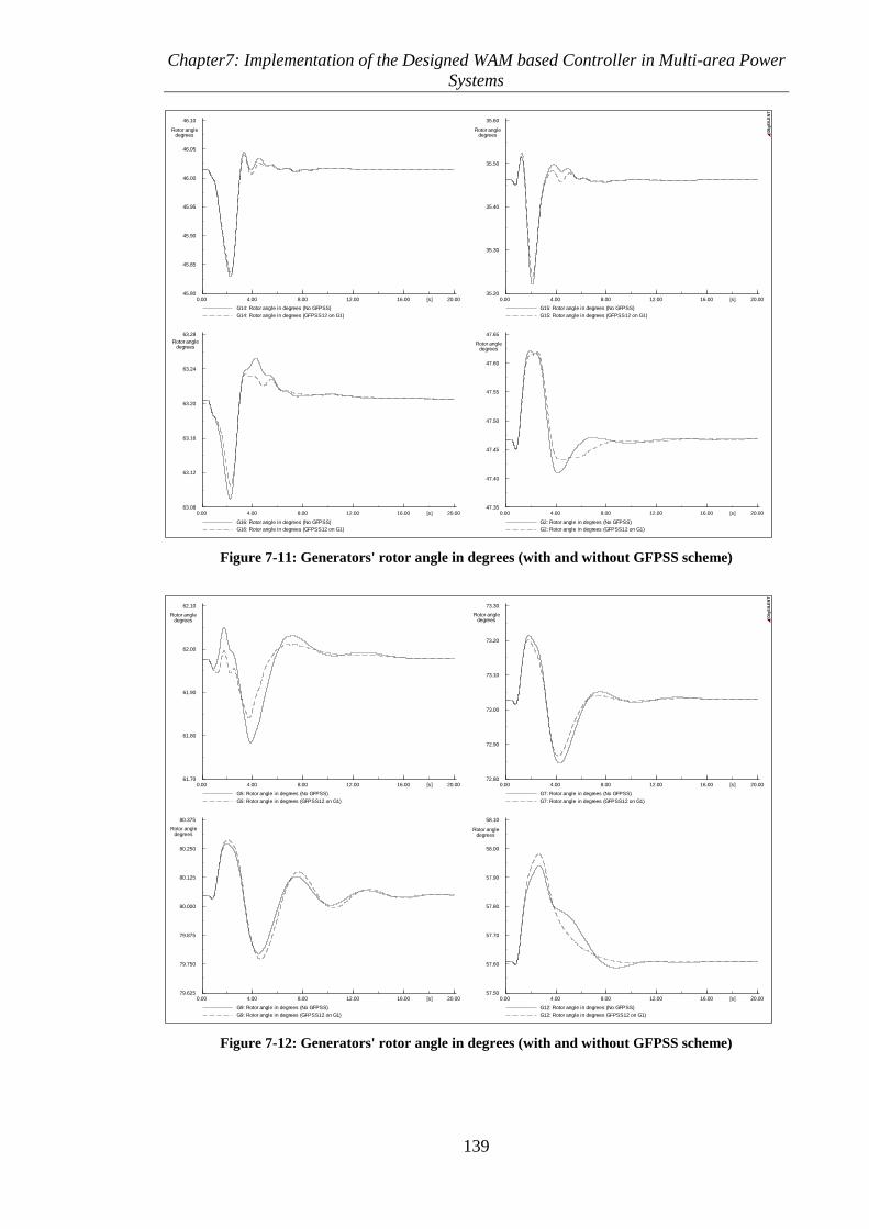
Chapter7: Implementation of the Designed WAM based Controller in Multi-area Power
Systems
139
20.0016.0012.008.004.000.00 [s]
46.10
46.05
46.00
45.95
45.90
45.85
45.80
G14: Rotor angle in degrees (No GFPSS)
G14: Rotor angle in degrees (GFPSS12 on G1)
20.0016.0012.008.004.000.00 [s]
35.60
35.50
35.40
35.30
35.20
G15: Rotor angle in degrees (No GFPSS)
G15: Rotor angle in degrees (GFPSS12 on G1)
20.0016.0012.008.004.000.00 [s]
63.28
63.24
63.20
63.16
63.12
63.08
G16: Rotor angle in degrees (No GFPSS)
G16: Rotor angle in degrees (GFPSS12 on G1)
20.0016.0012.008.004.000.00 [s]
47.65
47.60
47.55
47.50
47.45
47.40
47.35
G2: Rotor angle in degrees (No GFPSS)
G2: Rotor angle in degrees (GFPSS12 on G1)
Rotor angledegrees
Rotor angledegrees
Rotor angledegrees
Rotor angledegrees
DIg
SIL
EN
T
Figure 7-11: Generators' rotor angle in degrees (with and without GFPSS scheme)
20.0016.0012.008.004.000.00 [s]
80.375
80.250
80.125
80.000
79.875
79.750
79.625
G9: Rotor angle in degrees (No GFPSS)
G9: Rotor angle in degrees (GFPSS12 on G1)
20.0016.0012.008.004.000.00 [s]
73.30
73.20
73.10
73.00
72.90
72.80
G7: Rotor angle in degrees (No GFPSS)
G7: Rotor angle in degrees (GFPSS12 on G1)
20.0016.0012.008.004.000.00 [s]
62.10
62.00
61.90
61.80
61.70
G5: Rotor angle in degrees (No GFPSS)
G5: Rotor angle in degrees (GFPSS12 on G1)
20.0016.0012.008.004.000.00 [s]
58.10
58.00
57.90
57.80
57.70
57.60
57.50
G12: Rotor angle in degrees (No GFPSS)
G12: Rotor angle in degrees GFPSS12 on G1)
Rotor angledegrees
Rotor angledegrees
Rotor angledegrees
Rotor angledegrees
DIg
SIL
EN
T
Figure 7-12: Generators' rotor angle in degrees (with and without GFPSS scheme)

Chapter7: Implementation of the Designed WAM based Controller in Multi-area Power
Systems
140
Figures (7-13) and (7-14) give support evidence to what has been described as overall
system performance. The first, figure (7-13), shows enhanced transfer stability across
the transmission corridor connecting cluster 2 and 5 (line 50-51) when using the GFPSS
scheme. These results are supported by the second figure; figure (7-14), which shows
the difference in the weighted average speed deviation signals between cluster 2 and
cluster 5 during the disturbance. Notice the oscillatory unstable response when directing
the remote GFPSS signals to all units (bottom right graphs of both figures (7-13) and (7-
14)).
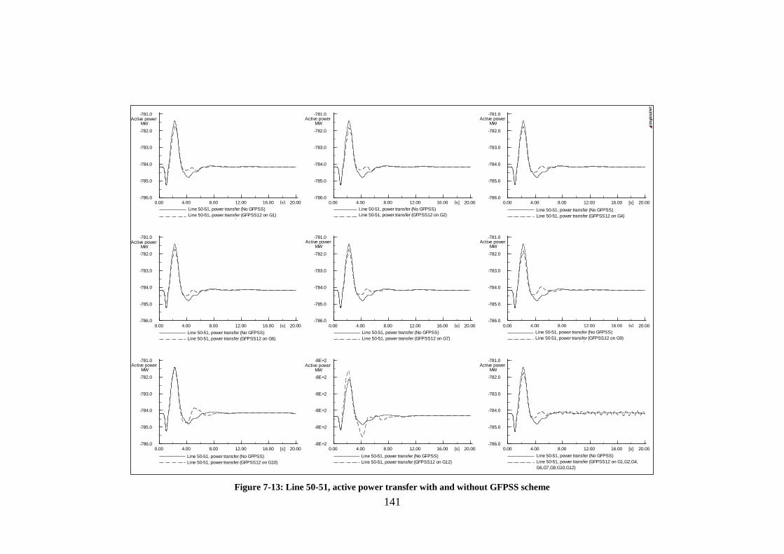
141
20.0016.0012.008.004.000.00 [s]
-781.0
-782.0
-783.0
-784.0
-785.0
-786.0
A25 Ptie deviation G1: p
A25 Ptie deviation G1: p
20.0016.0012.008.004.000.00 [s]
-781.0
-782.0
-783.0
-784.0
-785.0
-786.0
A25 Ptie deviation G1: p
A25 Ptie deviation G1: p
20.0016.0012.008.004.000.00 [s]
-781.0
-782.0
-783.0
-784.0
-785.0
-786.0
A25 Ptie deviation G1: p
A25 Ptie deviation G1: p
20.0016.0012.008.004.000.00 [s]
-8E+2
-8E+2
-8E+2
-8E+2
-8E+2
-8E+2
A25 Ptie deviation G1: p
A25 Ptie deviation G1: p
20.0016.0012.008.004.000.00 [s]
-781.0
-782.0
-783.0
-784.0
-785.0
-786.0
A25 Ptie deviation G1: p
A25 Ptie deviation G1: p
20.0016.0012.008.004.000.00 [s]
-781.0
-782.0
-783.0
-784.0
-785.0
-786.0
A25 Ptie deviation G1: p
A25 Ptie deviation G1: p
20.0016.0012.008.004.000.00 [s]
-781.0
-782.0
-783.0
-784.0
-785.0
-786.0
A25 Ptie deviation G1: p
A25 Ptie deviation G1: p
20.0016.0012.008.004.000.00 [s]
-781.0
-782.0
-783.0
-784.0
-785.0
-786.0
A25 Ptie deviation G1: p
A25 Ptie deviation G1: p
20.0016.0012.008.004.000.00 [s]
-781.0
-782.0
-783.0
-784.0
-785.0
-786.0
A25 Ptie deviation G1: p
A25 Ptie deviation G1: p
Line 50-51, power transfer (No GFPSS)
Line 50-51, power transfer (GFPSS12 on G1)
Line 50-51, power transfer (No GFPSS)
Line 50-51, power transfer (GFPSS12 on G2)Line 50-51, power transfer (No GFPSS)
Line 50-51, power transfer (GFPSS12 on G4)
Line 50-51, power transfer (No GFPSS)
Line 50-51, power transfer (GFPSS12 on G6)
Line 50-51, power transfer (No GFPSS)
Line 50-51, power transfer (GFPSS12 on G7)
Line 50-51, power transfer (No GFPSS)
Line 50-51, power transfer (GFPSS12 on G9)
Line 50-51, power transfer (No GFPSS)
Line 50-51, power transfer (GFPSS12 on G10)
Line 50-51, power transfer (No GFPSS)
Line 50-51, power transfer (GFPSS12 on G12)
Line 50-51, power transfer (No GFPSS)
Line 50-51, power transfer (GFPSS12 on G1,G2,G4,
G6,G7,G9,G10,G12)
Active powerMW
Active powerMW
Active powerMW
Active powerMW
Active powerMW
Active powerMW
Active powerMW
Active powerMW
Active powerMW D
IgS
ILE
NT
Figure 7-13: Line 50-51, active power transfer with and without GFPSS scheme

142
20.0016.0012.008.004.000.00 [s]
0.0010
0.0005
0.0000
-0.0005
-0.0010
-0.0015
A25 Speed Difference G1: dw
A25 Speed Difference G1: dw
20.0016.0012.008.004.000.00 [s]
0.0010
0.0005
0.0000
-0.0005
-0.0010
-0.0015
A25 Speed Difference G1: dw
A25 Speed Difference G1: dw
20.0016.0012.008.004.000.00 [s]
0.0010
0.0005
0.0000
-0.0005
-0.0010
-0.0015
A25 Speed Difference G1: dw
A25 Speed Difference G1: dw
20.0016.0012.008.004.000.00 [s]
0.0010
0.0005
0.0000
-0.0005
-0.0010
-0.0015
A25 Speed Difference G1: dw
A25 Speed Difference G1: dw
20.0016.0012.008.004.000.00 [s]
0.0010
0.0005
0.0000
-0.0005
-0.0010
-0.0015
A25 Speed Difference G1: dw
A25 Speed Difference G1: dw
20.0016.0012.008.004.000.00 [s]
0.0015
0.0010
0.0005
0.0000
-0.0005
-0.0010
-0.0015
A25 Speed Difference G1: dw
A25 Speed Difference G1: dw
20.0016.0012.008.004.000.00 [s]
0.0010
0.0005
0.0000
-0.0005
-0.0010
-0.0015
A25 Speed Difference G1: dw
A25 Speed Difference G1: dw
20.0016.0012.008.004.000.00 [s]
0.0010
0.0005
0.0000
-0.0005
-0.0010
-0.0015
A25 Speed Difference G1: dw
A25 Speed Difference G1: dw
20.0016.0012.008.004.000.00 [s]
0.0010
0.0005
0.0000
-0.0005
-0.0010
-0.0015
A25 Speed Difference G1: dw
A25 Speed Difference G1: dw
Speed dev.p.u
A25 speed deviation difference (No GFPSS)
A25 speed deviation difference (GFPSS12 on G1,G2,
G4,G6,G7,G9,G10,G12)
A25 speed deviation difference (No GFPSS)
A25 speed deviation difference (GFPSS12 on G1)
A25 speed deviation difference (No GFPSS)
A25 speed deviation difference (GFPSS12 on G9)
A25 speed deviation difference (No GFPSS)
A25 speed deviation difference (GFPSS12 on G7)
A25 speed deviation difference (No GFPSS)
A25 speed deviation difference (GFPSS12 on G6)
A25 speed deviation difference (No GFPSS)
A25 speed deviation difference (GFPSS12 on G4)
A25 speed deviation difference (No GFPSS)
A25 speed deviation difference (GFPSS12 on G2)
A25 speed deviation difference (No GFPSS)
A25 speed deviation difference (GFPSS12 on G12)
A25 speed deviation difference (No GFPSS)
A25 speed deviation difference (GFPSS12 on G10)
Speed dev.p.u
Speed dev.p.u
Speed dev.p.u
Speed dev.p.u
Speed dev.p.u
Speed dev.p.u
Speed dev.p.u
Speed dev.p.u
DIg
SIL
EN
T
Figure 7-14: Speed deviation difference between cluster 2 and 5 with and without GFPSS scheme

Chapter7: Implementation of the Designed WAM based Controller in Multi-area Power
Systems
143
B. Performance during large disturbances
Power systems are subject to large disturbances on daily bases. Those disturbances
include faults, units’ outages, tripping of a transmission line or any other types of
disturbances. The cause of these disturbances varies from human errors, equipment
failures or natural causes. It is, therefore, important to investigate the performance of
newly developed controllers under such circumstances. Hence, in order to have a
complete assessment of the performance of the developed GFPSS, the robustness and
the good performance during large disturbances and rabid changes in system operation
conditions are other criteria that have to be considered. For the system under
consideration, a number of scenarios are put into place to cover a wide range of possible
disturbances which may occur in any given power system.
The first scenario is a tripping of a heavily loaded transmission line (line 17-18, see
figure (7-2)). The line is tripped after 0.5 sec from the start of the simulation and the
response of the system to this large disturbance is monitored for a period of 20 sec with
the implementations of different configurations to the control scheme. Figure (7-15)
shows active power transfer between different clusters in the system following tripping
of the mentioned line. The top left graph gives active power transfer between clusters 2
and 4 (line 46-49), the top right graph gives active power transfer between clusters 2
and 5 (line 50-51), the bottom left graph gives power transfer between clusters 3 and 4
(line 41-42) and, finally, the bottom right graph gives active power transfer between
clusters 4 and 5 (line 42-52). Four different configurations for the control scheme are
considered in this scenario. Those configurations are as follows:
No GFPSS signal dispatch (the solid black line), GFPSS12 signal dispatch to generator
G1 in cluster 1 (the red dotted line), GFPSS12 signal dispatch to generators G1, G2 and
G4 in cluster 1 (the green dotted line) and GFPSS12 signal dispatch to generators G1,
G2, G4 and G9 in cluster 1 (the blue dotted line). As can be seen from figure (7-15),
following the tripping of the transmission line (line 17-18) oscillations occur in the
system as shown in the active power signals. However the oscillations seem to die out
after a period of time and the system regains a stable equilibrium condition.
Nonetheless, the effectiveness in damping those oscillations in different parts of the
network varies based on the used control scheme. As mentioned previously, damping

Chapter7: Implementation of the Designed WAM based Controller in Multi-area Power
Systems
144
power oscillations more effectively influences significantly the capability of power
systems to transfer higher amounts of power across the transmission network. If power
oscillations damping capabilities are enhanced, this increases security and reliability and
allows for better utilisation of power systems.
20.0016.0012.008.004.000.00 [s]
-382.0
-384.0
-386.0
-388.0
-390.0
-392.0
A24 Ptie deviation G1: p
A24 Ptie deviation G1: p
A24 Ptie deviation G1: p
A24 Ptie deviation G1: p
20.0016.0012.008.004.000.00 [s]
-780.0
-782.0
-784.0
-786.0
-788.0
A25 Ptie deviation G1: p
A25 Ptie deviation G1: p
A25 Ptie deviation G1: p
A25 Ptie deviation G1: p
20.0016.0012.008.004.000.00 [s]
-74.0
-75.0
-76.0
-77.0
-78.0
-79.0
A45 Ptie deviation G1: p
A45 Ptie deviation G1: p
A45 Ptie deviation G1: p
A45 Ptie deviation G1: p
20.0016.0012.008.004.000.00 [s]
77.50
76.25
75.00
73.75
72.50
71.25
A34 Ptie deviation G1: p
A34 Ptie deviation G1: p
A34 Ptie deviation G1: p
A34 Ptie deviation G1: p
Line 46-49, power transfer (No GFPSS)
Line 46-49, power transfer (GFPSS12 on G1)
Line 46-49, power transfer (GFPSS12 on G1,G2,G4)
Line 46-49, power transfer (GFPSS12 on G1,G2,G4,G9)
Line 50-51, power transfer (No GFPSS)
Line 50-51, power transfer (GFPSS12 on G1)
Line 50-51, power transfer (GFPSS12 on G1,G2,G4)
Line 50-51, power transfer (GFPSS12 on G1,G2,G4,G9)
Line 41-42, power transfer (No GFPSS)
Line 41-42, power transfer (GFPSS12 on G1)
Line 41-42, power transfer (GFPSS12 on G1.G2,G4)
Line 41-42, power transfer (GFPSS12 on G1,G2,G4,G9)
Line 42-52, power transfer (No GFPSS)
Line 42-52, power transfer (GFPSS12 on G1)
Line 42-52, power transfer (GFPSS12 on G1,G2,G4)
Line 42-52, power transfer (GFPSS12 on G1,G2,G4,G9)
Active powerMW
Active powerMW
Active powerMW
Active powerMW
DIg
SIL
EN
T
Figure 7-15: Active power transfer between different areas following tripping of line 17-18
The figure shows the robustness of the GFPSS scheme when added to the local
stabilisers. It shows that oscillations are damped best when the GFPSS signals are
dispatched to the four selected units (the blue dotted line). It also shows that even in the
case of, say failure of GFPSS signal to reach one of the four units, the control scheme
can still perform well. The advantages of being able to select a number of units to which
the GFPSS signal could be dispatched gives a degree of flexibility to the control scheme
and allows it to be robust and efficient.
The influence of the GFPSS scheme on the response of some of the individual units
within the system is illustrated in figures (7-16) and (7-17). The two figures show the
dynamic response of generators G14 and G15 (figure (7-16)) and generators G12 and

Chapter7: Implementation of the Designed WAM based Controller in Multi-area Power
Systems
145
G16 (figure (7-17)) by monitoring the trajectories which their rotor angles take
following the tripping of line 17-18.
20.0016.0012.008.004.000.00 [s]
46.20
46.10
46.00
45.90
45.80
G14: Rotor angle in degrees (No GFPSS)
G14: Rotor angle in degrees (GFPSS12 on G1)
G14: Rotor angle in degrees (GFPSS12 on G1, G2, G4)
G14: Rotor angle in degrees (GFPSS12 on G1, G2, G4, G9)
20.0016.0012.008.004.000.00 [s]
35.70
35.60
35.50
35.40
35.30
35.20
G15: Rotor angle in degrees (No GFPSS)
G15: Rotor angle in degrees (GFPSS12 on G1)
G15: Rotor angle in degrees (GFPSS12 on G1, G2, G4)
G15: Rotor angle in degrees (GFPSS12 on G1, G2, G4, G9)
Rotor angledegrees
Rotor angledegrees
DIg
SIL
EN
T
Figure 7-16: Generators' rotor angle in degrees (trip of line 17-18)
20.0016.0012.008.004.000.00 [s]
57.875
57.750
57.625
57.500
57.375
57.250
57.125
G12: Rotor angle in degrees (No GFPSS)
G12: Rotor angle in degrees (GFPSS12 on G1)
G12: Rotor angle in degrees (GFPSS12 on G1, G2, G4)
G12: Rotor angle in degrees (GFPSS12 on G1, G2, G4, G9)
20.0016.0012.008.004.000.00 [s]
63.40
63.30
63.20
63.10
63.00
G16: Rotor angle in degrees (No GFPSS)
G16: Rotor angle in degrees (GFPSS12 on G1)
G16: Rotor angle in degrees (GFPSS12 on G1, G2, G4)
G16: Rotor angle in degrees (GFPSS12 on G1, G2, G4, G9)
Rotor angledegrees
Rotor angledegrees
DIg
SIL
EN
T
Figure 7-17: Generators' rotor angle in degrees (trip of line 17-18)

Chapter7: Implementation of the Designed WAM based Controller in Multi-area Power
Systems
146
The superior performance of the GFPSS scheme is evident in both figures. Dispatching
the GFPSS signal to at least one of the selected units allowed other units in widely
spread area to regain stable operation following what is considered as a large
disturbance in the system.
The second scenario is a tripping of another transmission line (line 16-17, see figure (7-
2)). The line is tripped after 0.5 sec from the start of the simulation and the response of
the system to this large disturbance is monitored for a period of 20 sec with the
implementations of different configurations to the control scheme. The configurations
of the GFPSS dispatch signal scheme is slightly different to the one in the previous case
to illustrate the flexibility available for selectivity. Figures (7-18) and (7-19) show
power transfer between the five clusters in the system (line 8-9 power transfer between
cluster 1 and 2, line 1-47 power transfer between cluster 2 and 3, line 46-49 power
transfer between cluster 2 and 4, line 50-51 power transfer between cluster 2 and 5, line
41-42 power transfer between cluster 3 and 4 and line 42-52 power transfer between
cluster 4 and 5, refer to figure (7-2) for the network topology).
The GFPSS configuration considered in figure (7-18) are:
GFPSS12 signal dispatch to generator G1 (red dotted line), GFPSS12 signal dispatch to
a combination of G1 and G10 (blue dotted line); both are compared with no GFPSS
signal dispatch (solid black line).
On the other hand, in figure (7-19) different GFPSS dispatch strategies are considered
and those are:
GFPSS12 signal dispatch to a combination of G1 and G9 (red dotted line), GFPSS12
signal dispatch to G1, G2, G4 and G10 (blue dotted line), and again both control
strategies are with comparison to no elimination of the GFPSS from the control scheme
(no GFPSS).

147
20.0016.0012.008.004.000.00 [s]
-30.0
-60.0
-90.0
-120.0
-150.0
-180.0
A12 Ptie deviation G1: p
A12 Ptie deviation G1: p
A12 Ptie deviation G1: p
20.0016.0012.008.004.000.00 [s]
-160.0
-170.0
-180.0
-190.0
-200.0
-210.0
A23 Ptie deviation G1: p
A23 Ptie deviation G1: p
A23 Ptie deviation G1: p
20.0016.0012.008.004.000.00 [s]
-360.0
-370.0
-380.0
-390.0
-400.0
A24 Ptie deviation G1: p
A24 Ptie deviation G1: p
A24 Ptie deviation G1: p
20.0016.0012.008.004.000.00 [s]
-760.0
-770.0
-780.0
-790.0
A25 Ptie deviation G1: p
A25 Ptie deviation G1: p
A25 Ptie deviation G1: p
20.0016.0012.008.004.000.00 [s]
90.0
85.0
80.0
75.0
70.0
65.0
A34 Ptie deviation G1: p
A34 Ptie deviation G1: p
A34 Ptie deviation G1: p
20.0016.0012.008.004.000.00 [s]
-72.0
-75.0
-78.0
-81.0
-84.0
-87.0
A45 Ptie deviation G1: p
A45 Ptie deviation G1: p
A45 Ptie deviation G1: p
Active powerMW
Line 8-9, power transfer (No GFPSS)
Line 8-9, power transfer (GFPSS12 on G1)
Line 8-9, power transfer (GFPSS12 on G1, G10)
Line 50-51, power transfer (No GFPSS)
Line 50-51, power transfer (GFPSS12 on G1)
Line 50-51, power transfer (GFPSS12 on G1, G10)
Line 41-42, power transfer (No GFPSS)
Line 41-42, power transfer (GFPSS12 on G1)
Line 41-42, power transfer (GFPSS12 on G1, G10)
Line 42-52, power transfer (No GFPSS)
Line 42-52, power transfer (GFPSS12 on G1)
Line 42-52, power transfer (GFPSS12 on G1, G10)
Line 46-49, power transfer (No GFPSS)
Line 46-49, power transfer (GFPSS12 on G1)
Line 46-49, power transfer (GFPSS12 on G1, G10)
Line 1-47, power transfer (No GFPSS)
Line 1-47, power transfer (GFPSS12 on G1)
Line 1-47, power transfer (GFPSS12 on G1, G10)
Active powerMW
Active powerMW
Active powerMW
Active powerMW
Active powerMW D
IgS
ILE
NT
Figure 7-18: Active power transfer between different areas following tripping of line 16-17

148
20.0016.0012.008.004.000.00 [s]
-30.0
-60.0
-90.0
-120.0
-150.0
-180.0
A12 Ptie deviation G1: p
A12 Ptie deviation G1: p
A12 Ptie deviation G1: p
20.0016.0012.008.004.000.00 [s]
-160.0
-170.0
-180.0
-190.0
-200.0
-210.0
A23 Ptie deviation G1: p
A23 Ptie deviation G1: p
A23 Ptie deviation G1: p
20.0016.0012.008.004.000.00 [s]
-360.0
-370.0
-380.0
-390.0
-400.0
A24 Ptie deviation G1: p
A24 Ptie deviation G1: p
A24 Ptie deviation G1: p
20.0016.0012.008.004.000.00 [s]
-760.0
-770.0
-780.0
-790.0
A25 Ptie deviation G1: p
A25 Ptie deviation G1: p
A25 Ptie deviation G1: p
20.0016.0012.008.004.000.00 [s]
90.0
85.0
80.0
75.0
70.0
65.0
A34 Ptie deviation G1: p
A34 Ptie deviation G1: p
A34 Ptie deviation G1: p
20.0016.0012.008.004.000.00 [s]
-72.5
-75.0
-77.5
-80.0
-82.5
-85.0
-87.5
A45 Ptie deviation G1: p
A45 Ptie deviation G1: p
A45 Ptie deviation G1: p
Active powerMW
Active powerMW
Active powerMW
Active powerMW
Active powerMW
Active powerMW
Line 8-9, power transfer (No GFPSS)
Line 8-9, power transfer (GFPSS12 on G1,G9)
Line 8-9, power transfer (GFPSS12 on G1,G2,G4,G10)
Line 1-47, power transfer (No GFPSS)
Line 1-47, power transfer (GFPSS12 on G1,G9)
Line 1-47, power transfer (GFPSS12 on G1,G2,G4,G10)
Line 46-49, power transfer (No GFPSS)
Line 46-49, power transfer (GFPSS12 on G1,G9)
Line 46-49, power transfer (GFPSS12 on G1,G2,G4,G10)
Line 50-51, power transfer (No GFPSS)
Line 50-51, power transfer (GFPSS12 on G1,G9)
Line 50-51, power transfer (GFPSS12 on G1,G2,G4,G10)
Line 41-42, power transfer (No GFPSS)
Line 41-42, power transfer (GFPSS12 on G1.G9)
Line 41-42, power transfer (GFPSS12 on G1,G2,G4,G10)
Line 42-52, power transfer (No GFPSS)
Line 42-52, power transfer (GFPSS12 on G1,G9)
Line 42-52, power transfer (GFPSS12 on G1,G2,G4,G10)
DIg
SIL
EN
T
Figure 7-19: Active power transfer between different areas following tripping of line 16-17

Chapter7: Implementation of the Designed WAM based Controller in Multi-area Power
Systems
149
From both figures and given a variety of GFPSS signal dispatch configurations, it can
be seen that the added stabilising signals provided by the GFPSS resulted in an
enhanced overall system performance. The addition of the global control signal which is
produced based on wide-area information collected by the wide-area based global
stabiliser allowed local controllers to act based on a wider view to the entire system.
Hence, preventing wide spread system oscillations becomes more applicable and better
utilisation to the transmission assets is more visible and realistic.
Once more to evaluate the effectiveness of the GFPSS scheme, the response of
individual units to the disturbance under consideration is investigated. Figure (7-20)
gives the dynamic behaviour of two of the large units in the system G14 and G15
following the tripping of line 16-17 for different GFPSS signal dispatch strategies.
Three GFPSS configurations are illustrated in figure (7-20). Those are:
GFPSS12 signal dispatch to generator G1 (red dotted line), GFPSS signal dispatch to
generators G1, G2, G4 and G10(green dotted line), GFPSS signal dispatch to generators
G1, G2, G4, G6, G7, G9 and G10 (blue dotted line), all are plotted against the case with
no GFPSS inclusion in the control scheme (solid black line).
20.0016.0012.008.004.000.00 [s]
46.50
46.25
46.00
45.75
45.50
45.25
45.00
G14: Rotor angle in degrees (No GFPSS)
G14: Rotor angle in degrees (GFPSS12 on G1)
G14: Rotor angle in degrees (GFPSS12 on G1, G2, G4, G10)
G14: Rotor angle in degrees (GFPSS12 on G1, G2, G4, G6, G7, G9, G10)
20.0016.0012.008.004.000.00 [s]
36.40
36.00
35.60
35.20
34.80
34.40
34.00
G15: Rotor angle in degrees (No GFPSS)
G15: Rotor angle in degrees (GFPSS12 on G1)
G15: Rotor angle in degrees (GFPSS12 on G1, G2, G4, G10)
G15: Rotor angle in degrees (GFPSS12 on G1, G2, G4, G6, G7, G9, G10)
Rotor angledegrees
Rotor angledegrees
DIg
SIL
EN
T
Figure 7-20: Generators' rotor angle in degrees (trip of line 16-17)

Chapter7: Implementation of the Designed WAM based Controller in Multi-area Power
Systems
150
In the observations made for the two above scenarios considered for lines tripping, the
effectiveness of the proposed GFPSS in providing better overall system performance is
evident. The inclusion of the GFPSS control loop into the local control scheme of
individual units resulted in a significant enhancement to the stability of the transmission
system. Fewer oscillations with lower magnitudes are observed across the transmission
corridors across the entire system which means more power could be pushed through
theses corridors without risking the system security.
The third scenario for possible large disturbance is a three phase fault applied on one of
the bus-bars in the system. The system is subjected to a three phase fault of duration 50
ms on bus-bar 15 (see figure 7-2). Figure (7-21) shows active power transfer across line
8-9 connecting cluster 1 and cluster 2; the GFPSS12 stabilising signal is being sent to an
individual unit in each graph as shown (the units with active local PSS in their local
control loops). The graph at the bottom right of figure (7-21) is when the GFPSS signal
is sent to all the units at the same time. As clearly shown in the top left graph of figure
(7-21), the oscillations in the active power transfer signal across line 8-9 are
controllably damped more effectively when an additional stabilising control signal is
included in the stabilisation control loop of generator G1 (the dotted line). The
additional wide-area based signal from the proposed GFPSS enabled the power system
to a robust response to the sever disturbance in comparison to the case when only local
PSS stabilisers are used (the solid line). Similar results are obtained when dispatching
the GFPSS signals to other individual units that have active local PSS operating in their
control schemes. The graph in the bottom right of figure (7-21), however, supports
some remarks made earlier when analysing the performance of the GFPSS scheme
during small disturbances. It shows that it is not desirable to apply the GFPSS scheme
to all units at the same time as this may result in oscillatory unstable response in the
system. A good implementation strategy would be implementing the GFPSS scheme in
a limited number of units to ensure that at least one unit is receiving the stabilising
signal from the GFPSS.

151
Active power MW
20.0016.0012.008.004.000.00 [s]
0.0
-100.0
-200.0
-300.0
-400.0
A12 Ptie deviation G1: p
A12 Ptie deviation G1: p
20.0016.0012.008.004.000.00 [s]
0.0
-100.0
-200.0
-300.0
-400.0
A12 Ptie deviation G1: p
A12 Ptie deviation G1: p
20.0016.0012.008.004.000.00 [s]
0.0
-100.0
-200.0
-300.0
-400.0
A12 Ptie deviation G1: p
A12 Ptie deviation G1: p
20.0016.0012.008.004.000.00 [s]
0.0
-100.0
-200.0
-300.0
-400.0
A12 Ptie deviation G1: p
A12 Ptie deviation G1: p
20.0016.0012.008.004.000.00 [s]
0.0
-100.0
-200.0
-300.0
-400.0
A12 Ptie deviation G1: p
A12 Ptie deviation G1: p
20.0016.0012.008.004.000.00 [s]
0.0
-100.0
-200.0
-300.0
-400.0
A12 Ptie deviation G1: p
A12 Ptie deviation G1: p
20.0016.0012.008.004.000.00 [s]
0.0
-100.0
-200.0
-300.0
-400.0
A12 Ptie deviation G1: p
A12 Ptie deviation G1: p
20.0016.0012.008.004.000.00 [s]
0.0
-100.0
-200.0
-300.0
-400.0
A12 Ptie deviation G1: p
A12 Ptie deviation G1: p
20.0016.0012.008.004.000.00 [s]
0.0
-100.0
-200.0
-300.0
-400.0
A12 Ptie deviation G1: p
A12 Ptie deviation G1: p
Active powerMW
Active powerMW
Active powerMW
Active powerMW
Active power MW
Active powerMW
Active PowerMW
Active powerMW
Active powerMW
Line 8-9, power transfer (No GFPSS)
Line 8-9, power transfer (GFPSS12 on G1)
Line 8-9, power transfer (No GFPSS)
Line 8-9, power transfer (GFPSS12 on G2)
Line 8-9, power transfer (No GFPSS)
Line 8-9, power transfer (GFPSS12 on G6)
Line 8-9, power transfer (No GFPSS)
Line 8-9, power transfer (GFPSS12 on G4)
Line 8-9, power transfer (No GFPSS)
Line 8-9, power transfer (GFPSS12 on G7)
Line 8-9, power transfer (No GFPSS)
Line 8-9, power transfer (GFPSS12 on G9)
Line 8-9, power transfer (No GFPSS)
Line 8-9, power transfer (GFPSS12 on G1,G2,G4,G6,
G7,G9,G10,G12)
Line 8-9, power transfer (No GFPSS)
Line 8-9, power transfer (GFPSS12 on G12)
Line 8-9, power transfer (No GFPSS)
Line 8-9, power transfer (GFPSS12 on G10)
DIg
SIL
EN
T
Figure 7-21: Line 8-9, active power transfer (3 phase fault on BUS 15)

Chapter7: Implementation of the Designed WAM based Controller in Multi-area Power
Systems
152
As an example, figure (7-22) shows active power transfer signal across line 8-9 using
different GFPSS configurations. The top graph shows active power signals across the
transmission line when no GFPSS is used (black solid line), GFPSS12 signal dispatch to
G1 (dotted red line) and GFPSS12 signal dispatch to both G1 and G10 (dotted green
line). The bottom graph, on the other hand, shows similar control arrangement with the
exception of dispatching the additional control signal from the GFPSS to G1 and G12
rather than G1 and G10 in the top graph (dotted green line)
20.0016.0012.008.004.000.00 [s]
0.00
-100.00
-200.00
-300.00
-400.00
A12 Ptie deviation G1: p
A12 Ptie deviation G1: p
A12 Ptie deviation G1: p
20.0016.0012.008.004.000.00 [s]
0.00
-100.00
-200.00
-300.00
-400.00
A12 Ptie deviation G1: p
A12 Ptie deviation G1: p
A12 Ptie deviation G1: p
Line 8-9, power transfer (No GFPSS)
Line 8-9, power transfer (GFPSS12 on G1)
Line 8-9, power transfer (GFPSS12 on G1, G10)
Line 8-9, power transfer (No GFPSS)
Line 8-9, power transfer (GFPSS12 on G1)
Line 8-9, power transfer (GFPSS12 on G1, G12)
Active powerMW
Active powerMW
DIg
SIL
EN
T
Figure 7-22: Line 8-9, active power transfer (3 phase fault on BUS 15)
The response of two individual units to the control arrangement described above (no
GFPSS, GFPSS12 on G1 and GFPSS12 on G1 and G10) is illustrated in figure (7-23)
which shows the rotor angles of generators G15 in cluster 5 and G16 in cluster 4. The
top graph shows the swings in the rotor angle of generator G15 following the
disturbance. The improved performance of the stability control scheme is obvious when
comparing the two GFPSS arrangements (dotted red and blue lines) with that without
implementation of the GFPSS control loop. The swings in the rotor angle are damped
more effectively when incorporating the GFPSS signal into the control arrangement.

Chapter7: Implementation of the Designed WAM based Controller in Multi-area Power
Systems
153
20.0016.0012.008.004.000.00 [s]
36.25
35.00
33.75
32.50
31.25
30.00
G15: Rotor angle in degrees (No GFPSS)
G15: Rotor angle in degrees (GFPSS12 on G1)
G15: Rotor angle in degrees (GFPSS12 on G1, G10)
20.0016.0012.008.004.000.00 [s]
64.00
63.00
62.00
61.00
60.00
59.00
G16: Rotor angle in degrees (No GFPSS)
G16: Rotor angle in degrees (GFPSS12 on G1)
G16: Rotor angle in degrees (GFPSS12 on G1, G10)
Rotor angledegrees
Rotor angledegrees
DIg
SIL
EN
T
Figure 7-23: Generators' rotor angle in degrees (3 phase fault on BUS 15)
Similar observations can be made for generator G16 (bottom graph). This implies that
using global signals fetched from remote parts of the network and implementing these
signals to as inputs to newly designed control schemes can improve the damping of
rotor angle oscillations at the local units or plants as well as improving the damping of
power oscillations across interconnected areas and clusters in power systems.
7.2. Case Study 2: IEEE 39 Bus 2-Area Test System
The standard IEEE 10 generators 39-bus system consists 10 of generation units
interconnected via high voltage transmission lines. The system is used previously in
chapter 4 (section 4.3.2) as a study case to evaluate the clustering algorithm developed
to determine coherent clusters in large interconnected power systems. As described in
chapter 4, the system is formed of two coherent clusters connected via a transmission
line; the line connecting BUS16 and BUS19 (line 16-19) as shown in figure (7-24).
Since it is two clusters system, implementation of a single GFPSS control scheme that
act as a supervisory controller between those two clusters is a visible arrangement. The
input signals to this stability control scheme is derived from wide-area signals from

Chapter7: Implementation of the Designed WAM based Controller in Multi-area Power
Systems
154
across the entire system, namely, the differences in the weighted average speed
deviation signals of the units in both clusters and the deviations in the active power
transfer across the transmission line connecting both clusters (line 16-19). The
acquisitions of those signals are described by equations (6.9) to (6.11). The system is
modelled using the dynamic simulation programme DIgSILENT (Digital Simulator for
Electric Network). All generation units are equipped with continuous stability control
schemes that consist of excitation systems controls, speed governor controls and power
system stabilisers. The GFPSS scheme is implemented taking into account some of the
observations made in the previous study case. The GFPSS signal will only be applied to
few selected units as it is shown that dispatching the GFPSS signal to all units at once
has a rather negative impact on the stability of the system. In this case, generator G1
will be the focus of the GFPSS scheme, being the reference and largest unit in the
system. Other units are generator G7 and G8 which are selected based on extensive
simulations that led to conclude that the control scheme works best when those units are
considered. Similarly to the previous case, the controller performance is tested for both
small disturbances and large disturbances during a number of operating scenarios.

155
Cluster 1
Cluster 2
G ~
G9
G~G6
G~
G7G~ G3
G~
G2
G ~ G8
G~
G1
G~
G10
0
0
0
0
0
0
0
0
0
0
0
0
G~ G5
G~G4
BUS19
BUS36
BUS23
BUS35
BUS38
BUS22BUS21
BUS32
BUS3
BUS18
BUS26
BUS25
BUS37
BUS9
BUS39
BUS24
BUS16
BUS15
BUS13
BUS10
BUS11
BUS12
BUS31
BUS1
BUS14
BUS17
BUS27
BUS29BUS28
BUS8
BUS7
BUS6
BUS5
BUS4
BUS2
BUS30
BUS33BUS34
BUS20
DIg
SIL
EN
T
Figure 7-24: IEEE 10 machines 39 bus / two clusters system

Chapter7: Implementation of the Designed WAM based Controller in Multi-area Power
Systems
156
A. Performance during small disturbances
For small signal disturbance, a pulse of 5% magnitude at the voltage reference of the
largest generator G1 located in cluster 1 for a time period of 50 ms. The system’s
response to this disturbance is then monitored under a variety of available control
arrangements. The system’s behaviour following the disturbance can be viewed in a
number of variables that display the dynamic response of the system during and
following the occurrence of the event. A good dynamic variable that can show the
response of the system based on the used control arrangement is the difference in the
weighted average speed deviation signal between cluster 1 and 2 as shown in figure (7-
25) bellow. The figure shows four different control arrangements with regard dispatch
of the control signal from the GFPSS. The top left graph is when GFPSS control signal
is applied to generator G1 (red dotted line), top right graph is when GFPSS control
signal is applied to generator G7 (red dotted line), bottom left graph is when GFPSS
control signal is applied to generator G8 (red dotted line) and bottom right graph is
when GFPSS control signal is applied to a combination of the three units at once G1,
G7 and G8 (red dotted line). The four control arrangements are compared to the base
case when there is no GFPSS controller in service (black solid line). The aim of the
stabilising control strategy is to minimise any oscillations in the system and to maintain
stable equilibrium point of operation in the shortest possible time. The GFPSS inclusion
into the control scheme seems to have achieved those goals as can be seen from the
figure. Best GFPSS control performance is obtained when the control signal is directed
to generator G1, being the largest reference unit in the system. A good system response
is also observed when directing the signal to either generator G7 or G8 as oscillations
are damped more effectively. Dispatching the signal to more than one unit at the same
time insures that at least one of these units receives the wide-area based control signal;
hence, provides the required additional damping force which is needed to enhance the
system’s stability.

Chapter7: Implementation of the Designed WAM based Controller in Multi-area Power
Systems
157
30.0020.0010.000.00 [s]
0.00003
0.00002
0.00001
0.00000
-0.00001
-0.00002
A12 Speed Difference G1: dw
A12 Speed Difference G1: dw
30.0020.0010.000.00 [s]
0.00002
0.00001
0.00000
-0.00001
A12 Speed Difference G1: dw
A12 Speed Difference G1: dw
30.0020.0010.000.00 [s]
0.00002
0.00001
0.00000
-0.00001
A12 Speed Difference G1: dw
A12 Speed Difference G1: dw
30.0020.0010.000.00 [s]
0.00002
0.00001
0.00000
-0.00001
-0.00002
A12 Speed Difference G1: dw
A12 Speed Difference G1: dw
A12 speed deviation difference (NO GFPSS)
A12 speed deviation difference (GFPSS12 on G1)
Speed dev.p.u
Speed dev.p.u
Speed dev.p.u
Speed dev.p.u
A12 speed deviation difference (NO GFPSS)
A12 speed deviation difference (GFPSS12 on G1, G7, G8)
A12 speed deviation difference (NO GFPSS)
A12 speed deviation difference (GFPSS12 on G8)
A12 speed deviation difference (NO GFPSS)
A12 speed deviation difference (GFPSS12 on G7)
DIg
SIL
EN
T
Figure 7-25: Speed deviation difference between cluster 1 and 2 (pulse on voltage reference of
generator G1)
Providing the additional damping to the system allows for better transfer capabilities.
This can be seen in the power transfer signals across the transmission system. Figure (7-
26) shows active power transfer across the transmission line connecting clusters 1 and 2
(line 18-19, see figure (7-24)). The figure follows similar control arrangements to that
described for figure (7-25). As oscillations between the two clusters are controllably
damped more quickly using the GFPSS arrangements, more power can be transferred
across the transmission system with a high degree of confidence in system’s security.
The GFPSS strategy increases the stability limits of the system which goes hand in hand
with security and reliability improvement. As a result, it allows for better utilisation and
more flexibility of the transmission networks, an important and necessary requirement
for today’s power system.

Chapter7: Implementation of the Designed WAM based Controller in Multi-area Power
Systems
158
30.0020.0010.000.00 [s]
-506.25
-506.30
-506.35
-506.40
-506.45
-506.50
A12 Ptie deviation G1: p
A12 Ptie deviation G1: p
30.0020.0010.000.00 [s]
-506.25
-506.30
-506.35
-506.40
-506.45
-506.50
A12 Ptie deviation G1: p
A12 Ptie deviation G1: p
30.0020.0010.000.00 [s]
-506.25
-506.30
-506.35
-506.40
-506.45
-506.50
A12 Ptie deviation G1: p
A12 Ptie deviation G1: p
30.0020.0010.000.00 [s]
-506.25
-506.30
-506.35
-506.40
-506.45
-506.50
A12 Ptie deviation G1: p
A12 Ptie deviation G1: p
Line 16-19, power transfer (NO GFPSS)
Line 16-19, power transfer (GFPSS12 on G1)
Active powerMW
Active powerMW
Active powerMW
Active powerMW
Line 16-19, power transfer (NO GFPSS)
Line 16-19, power transfer (GFPSS12 on G1, G7, G8)
Line 16-19, power transfer (NO GFPSS)
Line 16-19, power transfer (GFPSS12 on G8)
Line 16-19, power transfer (NO GFPSS)
Line 16-19, power transfer (GFPSS12 on G7)
DIg
SIL
EN
T
Figure 7-26: Line 16-19, active power transfer (pulse on voltage reference of G1)
To evaluate the impact of the GFPSS different arrangements on individual units in the
system, figure (7-27) displays the dynamic response of generator G1 to the encountered
disturbance. The response of the unit is captured in the trajectory which its rotor angle
follows following the disturbance. The figure shows the unit response when the GFPSS
signal is dispatched to three different individual units each time. The graph in the top is
when the GFPSS signal is sent to G1, the graph in the middle is when the GFPSS signal
is sent to G7 and the graph in the bottom is when the GFPSS signal is sent to G8 (all
responses are illustrated in red dotted lines). Again, the three cases are compared with
the base case when no GFPSS controller is put into service (the black solid lines). As
can be seen from the figure, the rotor angle of the largest unit in the system seems to
swing less (both in magnitude and duration) when there is a GFPSS controller acting
between the two clusters in the system under study. The unit regains a stable
equilibrium point of operation very quickly. It also experiences fewer oscillations in the
kinetic energy stored in its rotor when a GFPSS control signal is sent to any of the
selected units. The unit response is also displayed when combinations of GFPSS signal
dispatch strategies to the selected generators are put into place; this is shown in figure
(7-28).

Chapter7: Implementation of the Designed WAM based Controller in Multi-area Power
Systems
159
30.0020.0010.000.00 [s]
-2.57
-2.58
-2.59
-2.60
-2.61
G1: Rotor angle (No GFPSS)
G1: Rotor angle (GFPSS on G1)
30.0020.0010.000.00 [s]
-2.57
-2.58
-2.59
-2.60
-2.61
G1: Rotor angle (No GFPSS)
G1: Rotor angle (GFPSS on G7)
30.0020.0010.000.00 [s]
-2.57
-2.58
-2.59
-2.60
-2.61
G1: Rotor angle (No GFPSS)
G1: Rotor angle (GFPSS on G8)
Rotor angledegrees
Rotor angledegrees
Rotor angledegrees
DIg
SIL
EN
T
Figure 7-27: Rotor angle of G1 in degrees (pulse on voltage reference of G1)
30.0020.0010.000.00 [s]
-2.57
-2.58
-2.59
-2.60
-2.61
G1: Rotor angle (No GFPSS)
G1: Rotor angle (GFPSS on G1, G7)
30.0020.0010.000.00 [s]
-2.57
-2.58
-2.59
-2.60
-2.61
G1: Rotor angle (No GFPSS)
G1: Rotor angle (GFPSS on G1, G7, G8)
30.0020.0010.000.00 [s]
-2.57
-2.58
-2.59
-2.60
-2.61
G1: Rotor angle (No GFPSS)
G1: Rotor angle (GFPSS on G1)
G1: Rotor angle (GFPSS on G1, G7)
G1: Rotor angle (GFPSS on G1, G7, G8)
Rotor angledegrees
Rotor angledegrees
Rotor angledegrees
DIg
SIL
EN
T
Figure 7-28: Rotor angle of G1 in degrees (pulse on voltage reference of G1)

Chapter7: Implementation of the Designed WAM based Controller in Multi-area Power
Systems
160
The top graph in figure (7-28) shows the rotor response of G1 when GFPSS signals are
applied to both G1 and G7, the middle graph is when the GFPSS signal is applied to a
combination G1, G7 and G8 and the bottom graph plots latter control arrangements with
the case when a GFPSS signal is applied to G1. The black solid line is always for the
base case when there is no active GFPSS. With comparison to the case when there is no
GFPSS active between the two clusters, it is clear that any control arrangement which
includes a GFPSS scheme into the stabilising loops of individual units would result in a
better system response and enhanced control performance.
B. Performance during large disturbances
The performance of the GFPSS scheme in this study case is also tested for large power
system disturbances and rabid sudden changes in system conditions to insure its
robustness and its satisfactory performance during such operating conditions. A number
of scenarios are considered to cover a wide range of possible disturbances which may
occur in any real power system. Included in this section is a case of a transmission line
outage and a case of a three phase fault at one of the system buses as will be explained.
The first scenario is a tripping of a transmission line (line 17-18, see figure (7-24)). The
line is tripped after 0.5 sec from the start of the simulation and the response of the
system to this large disturbance is monitored for a period of 30 sec with the
implementations of different configurations to the control scheme. The generators
considered for implementation of the GFPSS scheme are the same as for the case of
small disturbances explained above. Figure (7-29) shows the difference in the weighed
speed deviation signals between cluster 1 and 2. The top left graph gives the system
response when the GFPSS scheme is applied to generator G1, the top right graph is for
the system response when the GFPSS scheme is applied to generator G7, the bottom left
graph is for the system response when the GFPSS scheme is applied to generator G8
and the bottom right graph is for the system response when the GFPSS scheme is
applied to the three units combined G1, G7 and G8. The red dotted line in figure (7-29)
is for the system response when there is a GFPSS active and is compared with the case
when only local power system stabilisers are available at the local plant (the black solid
lines). With comparison to the case when only local PSS are acting to provide the

Chapter7: Implementation of the Designed WAM based Controller in Multi-area Power
Systems
161
stabilisation signal based on the locally available feedback signals, it is obvious that
adding the wide-area based GFPSS loop into the stabilisation control loop provides
more oscillation damping capabilities. This is clear for any GFPSS control arrangement
given in figure (7-29). The difference in the weighted speed deviation signals between
cluster 1 and 2 settle more quickly (it takes less time for the oscillations to damp out)
with fewer oscillations when there is a GFPSS scheme put into place.
30.0020.0010.000.00 [s]
0.002
0.000
-0.002
-0.004
-0.006
-0.008
A12 Speed Difference G1: dw
A12 Speed Difference G1: dw
30.0020.0010.000.00 [s]
0.002
0.000
-0.002
-0.004
-0.006
A12 Speed Difference G1: dw
A12 Speed Difference G1: dw
30.0020.0010.000.00 [s]
0.002
0.000
-0.002
-0.004
-0.006
A12 Speed Difference G1: dw
A12 Speed Difference G1: dw
30.0020.0010.000.00 [s]
0.004
0.002
0.000
-0.002
-0.004
-0.006
-0.008
A12 Speed Difference G1: dw
A12 Speed Difference G1: dw
A12 speed deviation difference (NO GFPSS)
A12 speed deviation difference (GFPSS12 on G1)
Speed dev.p.u
Speed dev.p.u
Speed dev.p.u
Speed dev.p.u
A12 speed deviation difference (NO GFPSS)
A12 speed deviation difference (GFPSS12 on G1, G7, G8)
A12 speed deviation difference (NO GFPSS)
A12 speed deviation difference (GFPSS12 on G8)
A12 speed deviation difference (NO GFPSS)
A12 speed deviation difference (GFPSS12 on G7)
DIg
SIL
EN
T
Figure 7-29: Speed deviation difference between cluster 1 and 2 (tripping of line 17-18)
The improvement in oscillation damping capabilities can also be seen in the signals of
active power transfer between the two clusters as shown in figure (7-30). The figure
shows active power transfer across the transmission line connecting cluster 1 and 2 (line
16-19). The control arrangement for this figure is the same as the one described above
for figure (7-28). The oscillations between the two clusters are controllably damped
more effectively using the GFPSS scheme. Being able to damp the oscillations between
wide spread connected areas improves the transmission stability and allows for better
exploitations for transmission assets. Figure (7-30) also shows that it is recommended to
have the GFPSS scheme implemented to at least 2 units in the system to provide a

Chapter7: Implementation of the Designed WAM based Controller in Multi-area Power
Systems
162
degree of certainty that the additional wide-area based control signal would be active at
one of the units.
30.0020.0010.000.00 [s]
-450.00
-462.50
-475.00
-487.50
-500.00
-512.50
-525.00
A12 Ptie deviation G1: p
A12 Ptie deviation G1: p
30.0020.0010.000.00 [s]
-450.00
-462.50
-475.00
-487.50
-500.00
-512.50
-525.00
A12 Ptie deviation G1: p
A12 Ptie deviation G1: p
30.0020.0010.000.00 [s]
-450.00
-462.50
-475.00
-487.50
-500.00
-512.50
-525.00
A12 Ptie deviation G1: p
A12 Ptie deviation G1: p
30.0020.0010.000.00 [s]
-450.00
-462.50
-475.00
-487.50
-500.00
-512.50
-525.00
A12 Ptie deviation G1: p
A12 Ptie deviation G1: p
Line 16-19, power transfer (NO GFPSS)
Line 16-19, power transfer (GFPSS12 on G1)
Active powerMW
Active powerMW
Active powerMW
Active powerMW
Line 16-19, power transfer (NO GFPSS)
Line 16-19, power transfer (GFPSS12 on G1, G7, G8)
Line 16-19, power transfer (NO GFPSS)
Line 16-19, power transfer (GFPSS12 on G8)
Line 16-19, power transfer (NO GFPSS)
Line 16-19, power transfer (GFPSS12 on G7)
DIg
SIL
EN
T
Figure 7-30: Line 16-19, active power transfer (tripping of line 17-18)
The response of the individual units the encountered disturbance is illustrated in figure
(7-31) and figure (7-32) bellow. Both figures show the rotor angles of the system’s units
in degrees. Figure (7-31) shows a comparison of the dynamic response of all units in the
system (G1 to G9) when the GFPSS control signal is added to the stabilisation control
loop of generator G1 (depicted by the red dotted lines) with the response of the units
when only local PSS are activated (shown by the black solid lines). As can be seen, the
oscillations in all units’ rotors seem to be enhanced significantly when a GFPSS scheme
is put into place to provide additional stabilising control signal through the excitation
system of generator G1. All units tend to regain stable operating equilibrium more
quickly following the tripping of the transmission line when the GFPSS signal is
dispatched. Considering, for example, the trajectory that the rotor angle of generator G1
takes (top left graph of figure (7-31)) as the disturbance occur and comparing the two
cases (with and without GFPSS), it is obvious the significant improvement that the
GFPSS scheme can provide when added to local control strategies.

163
30.0020.0010.000.00 [s]
-2.00
-2.40
-2.80
-3.20
-3.60
-4.00
G1: Rotor angle in degrees (NO GFPSS)
G1: Rotor angle in degrees (GFPSS12 on G1)
30.0020.0010.000.00 [s]
10.60
10.40
10.20
10.00
9.80
G2: Rotor angle in degrees (NO GFPSS)
G2: Rotor angle in degrees (GFPSS12 on G1)
Rotor angledegree
Time (s)
Time (s)Time (s)
30.0020.0010.000.00 [s]
24.00
23.00
22.00
21.00
20.00
19.00
G4: Rotor angle in degrees (NO GFPSS)
G4: Rotor angle in degrees (GFPSS12 on G1)
30.0020.0010.000.00 [s]
14.40
14.20
14.00
13.80
13.60
13.40
G3: Rotor angle in degrees (NO GFPSS)
G3: Rotor angle in degrees (GFPSS12 on G1)
30.0020.0010.000.00 [s]
37.00
36.00
35.00
34.00
33.00
32.00
G5: Rotor angle in degrees (NO GFPSS)
G5: Rotor angle in degrees (GFPSS12 on G1)
30.0020.0010.000.00 [s]
18.50
18.25
18.00
17.75
17.50
17.25
17.00
G8: Rotor angle in degrees (NO GFPSS)
G8: Rotor angle in degrees (GFPSS12 on G1)
30.0020.0010.000.00 [s]
25.00
24.00
23.00
22.00
21.00
20.00
G6: Rotor angle in degrees (NO GFPSS)
G6: Rotor angle in degrees (GFPSS12 on G1)
30.0020.0010.000.00 [s]
27.00
26.00
25.00
24.00
23.00
G7: Rotor angle in degrees (NO GFPSS)
G7: Rotor angle in degrees (GFPSS12 on G1)
30.0020.0010.000.00 [s]
22.50
22.00
21.50
21.00
20.50
20.00
19.50
G9: Rotor angle in degrees (NO GFPSS)
G9: Rotor angle in degrees (GFPSS12 on G1)
Rotor angledegree
Rotor angledegree
Rotor angledegree
Rotor angledegree
Rotor angledegree
Rotor angledegree
Rotor angledegree
Rotor angledegree
DIg
SIL
EN
T
Figure 7-31: Rotor angle of generators G1 to G9 in degrees (tripping of line 17-18 / GFPSS12 on G1)

164
30.0020.0010.000.00 [s]
-2.00
-2.40
-2.80
-3.20
-3.60
-4.00
G1: Rotor angle in degrees (NO GFPSS)
G1: Rotor angle in degrees (GFPSS12 on G7)
30.0020.0010.000.00 [s]
10.625
10.500
10.375
10.250
10.125
10.000
G2: Rotor angle in degrees (NO GFPSS)
G2: Rotor angle in degrees (GFPSS12 on G7)
Rotor angledegree
Time (s)
Time (s)Time (s)
30.0020.0010.000.00 [s]
24.00
23.00
22.00
21.00
20.00
19.00
G4: Rotor angle in degrees (NO GFPSS)
G4: Rotor angle in degrees (GFPSS12 on G7)
30.0020.0010.000.00 [s]
14.40
14.20
14.00
13.80
13.60
G3: Rotor angle in degrees (NO GFPSS)
G3: Rotor angle in degrees (GFPSS12 on G7)
30.0020.0010.000.00 [s]
37.00
36.00
35.00
34.00
33.00
32.00
G5: Rotor angle in degrees (NO GFPSS)
G5: Rotor angle in degrees (GFPSS12 on G7)
30.0020.0010.000.00 [s]
18.50
18.25
18.00
17.75
17.50
17.25
G8: Rotor angle in degrees (NO GFPSS)
G8: Rotor angle in degrees (GFPSS12 on G7)
30.0020.0010.000.00 [s]
25.00
24.00
23.00
22.00
21.00
20.00
G6: Rotor angle in degrees (NO GFPSS)
G6: Rotor angle in degrees (GFPSS12 on G7)
30.0020.0010.000.00 [s]
28.00
27.00
26.00
25.00
24.00
23.00
22.00
G7: Rotor angle in degrees (NO GFPSS)
G7: Rotor angle in degrees (GFPSS12 on G7)
30.0020.0010.000.00 [s]
22.50
22.00
21.50
21.00
20.50
20.00
19.50
G9: Rotor angle in degrees (NO GFPSS)
G9: Rotor angle in degrees (GFPSS12 on G7)
Rotor angledegree
Rotor angledegree
Rotor angledegree
Rotor angledegree
Rotor angledegree
Rotor angledegree
Rotor angledegree
Rotor angledegree
DIg
SIL
EN
T
Figure 7-32: Rotor angle of generators G1 to G9 in degrees (tripping of line 17-18 / GFPSS12 on G7)

Chapter7: Implementation of the Designed WAM based Controller in Multi-area Power
Systems
165
Similar observation can be made when monitoring the rotor angles of the system’s units
during the disturbance giving that the GFPSS scheme us applied to the control system
of generator G7 as shown in figure (7-32) with the exception of the response of
generator G7 itself. Nonetheless, as an overall system performance, the GFPSS scheme
seems to improve the stability of the system as a whole when applied to any of the
selected units as described in figure (7-29) and (7-30) above.
The second large disturbance scenario is a three phase fault applied on one of the bus-
bars in the system. The system is subjected to a three phase fault of duration 50 ms on
bus-bar 1 (BUS 1, see figure (7-24)). The dynamic response of the system to this large
disturbance is monitored for a period of 30 sec with the implementations of different
configurations to the GFPSS control scheme, similar to those considered in the previous
events (i.e. the GFPSS wide-area base control signal is dispatched to generators G1 or
G7 or G8 or to a their combination). Figure (7-33) shows active power transfer across
the transmission line (L9-36, see figure (7-24)).
30.0020.0010.000.00 [s]
10.00
0.00
-10.00
-20.00
-30.00
-40.00
Cub_1\PQ Meas L9-39: Active Power in p.u.
Cub_1\PQ Meas L9-39: Active Power in p.u.
30.0020.0010.000.00 [s]
10.00
0.00
-10.00
-20.00
-30.00
-40.00
Cub_1\PQ Meas L9-39: Active Power in p.u.
Cub_1\PQ Meas L9-39: Active Power in p.u.
30.0020.0010.000.00 [s]
10.00
0.00
-10.00
-20.00
-30.00
-40.00
Cub_1\PQ Meas L9-39: Active Power in p.u.
Cub_1\PQ Meas L9-39: Active Power in p.u.
30.0020.0010.000.00 [s]
10.00
0.00
-10.00
-20.00
-30.00
-40.00
Cub_1\PQ Meas L9-39: Active Power in p.u.
Cub_1\PQ Meas L9-39: Active Power in p.u.
Line 9-39, power transfer (NO GFPSS)
Line 9-39, power transfer (GFPSS12 on G1)
Active powerMW
Active powerMW
Active powerMW
Active powerMW
Line 9-39, power transfer (NO GFPSS)
Line 9-39, power transfer (GFPSS12 on G1, G7, G8)
Line 9-39, power transfer (NO GFPSS)
Line 9-39, power transfer (GFPSS12 on G8)
Line 9-39, power transfer (NO GFPSS)
Line 9-39, power transfer (GFPSS12 on G7)
DIg
SIL
EN
T
Figure 7-33: Line 9-36, active power transfer (3 phase fault on BUS 1)

Chapter7: Implementation of the Designed WAM based Controller in Multi-area Power
Systems
166
The black solid line represents active power transfer via the considered line when only
local stabilisers are available at the local stabilisation control loop of the generators. The
red dotted line, on the other hand, represents active power transfer across the
transmission line when a GFPSS control loop is added as a provider to a wide-area
based stabilising control signal to one or more of selected units. As can be seen from
figure (7-33), a considerable improvement in damping the oscillations in the
transmission corridor caused by the occurred fault is achieved as a result of the
additional stabilisation control loop (the GFPSS loop). The system stability following
the disturbance is enhanced regardless to which of the three units (G1, G7 and G8) the
GFPSS signal is sent. Dispatching the GFPSS signal to more than one selected unit
(bottom right graph in figure (7-33)) guarantees that the stabilisation effect on the
system will be assured since at least one of these units will receive the additional control
signal. The stabilising effect of the additional GFPSS loop can also be seen in the
difference in the weighted speed deviation signals between cluster 1 and 2, shown in
figure (7-34)
30.0020.0010.000.00 [s]
2.50E-4
1.25E-4
0.00E+0
-1.25E-4
-2.50E-4
-3.75E-4
A12 Speed Difference G1: dw
A12 Speed Difference G1: dw
30.0020.0010.000.00 [s]
0.0002
0.0001
0.0000
-0.0001
-0.0002
-0.0003
A12 Speed Difference G1: dw
A12 Speed Difference G1: dw
30.0020.0010.000.00 [s]
3.75E-4
2.50E-4
1.25E-4
0.00E+0
-1.25E-4
-2.50E-4
-3.75E-4
A12 Speed Difference G1: dw
A12 Speed Difference G1: dw
30.0020.0010.000.00 [s]
0.0004
0.0002
0.0000
-0.0002
-0.0004
A12 Speed Difference G1: dw
A12 Speed Difference G1: dw
A12 speed deviation difference (NO GFPSS)
A12 speed deviation difference (GFPSS12 on G1)
Speed dev.p.u
Speed dev.p.u
Speed dev.p.u
Speed dev.p.u
A12 speed deviation difference (NO GFPSS)
A12 speed deviation difference (GFPSS12 on G1, G7, G8)
A12 speed deviation difference (NO GFPSS)
A12 speed deviation difference (GFPSS12 on G8)
A12 speed deviation difference (NO GFPSS)
A12 speed deviation difference (GFPSS12 on G7)
DIg
SIL
EN
T
Figure 7-34: Speed deviation difference between cluster 1 and 2 (3 phase fault on BUS 1)

Chapter7: Implementation of the Designed WAM based Controller in Multi-area Power
Systems
167
The red dotted line represents the difference of the weighted average speed deviation
signals of the generators in cluster 1 and 2 derived based on equations (6.9) and (6.10)
when a GFPSS scheme is implemented and is compared with the case with no GFPSS
in place. The signals give an insight in how the generators in both clusters respond to
the disturbance. Figure (7-34) supports the observations made for figure (7-33) and it
also shows that better control arrangement is achieved when dispatching the GFPSS
signal to generator G1. Although implementing the GFPSS scheme on generators G7
and G8 is less effective than implementing it on G1, the overall performance of the
system is still better with the addition of the GFPSS control loop.
The superior performance of the GFPSS scheme when implemented on G1 can be seen
clearly in the speed deviation signals of the individual units shown in figure (7-35). The
figure shows the response of all units in the system (G1 to G9) when the GFPSS signal
is sent to generator G1 (the red dotted line) with comparison to the system’s response
with no additional GFPSS control loop (the solid black line). It can be seen that the
speed deviations of all units settles more quickly in a shorter time frame when
implementing the GFPSS scheme. This implies that all units in the system are able to
regain a stable post-fault operating equilibrium in a much improved manner with
comparison to the case with no GFPSS. The ability of all units to maintain their stable
equilibrium more effectively reflects positively on the overall performance of the
system as shown in figures (7-34) and (7-33).

168
30.0020.0010.000.00 [s]
0.0002
0.0001
0.0000
-0.0001
-0.0002
-0.0003
G1: Speed deviation (NO GFPSS)
G1: Speed deviation (GFPSS12 on G1)
30.0020.0010.000.00 [s]
0.00075
0.00050
0.00025
0.00000
-0.00025
-0.00050
G2: Speed deviation (NO GFPSS)
G2: Speed deviation (GFPSS12 on G1)
Speed dev.p.u
Time (s)
Time (s)Time (s)
30.0020.0010.000.00 [s]
0.0006
0.0004
0.0002
0.0000
-0.0002
-0.0004
G4: Speed deviation (NO GFPSS)
G4: Speed deviation (GFPSS12 on G1)
30.0020.0010.000.00 [s]
0.0006
0.0004
0.0002
0.0000
-0.0002
-0.0004
-0.0006
G3: Speed deviation (NO GFPSS)
G3: Speed deviation (GFPSS12 on G1)
30.0020.0010.000.00 [s]
0.0006
0.0004
0.0002
0.0000
-0.0002
-0.0004
G5: Speed deviation (NO GFPSS)
G5: Speed deviation (GFPSS12 on G1)
30.0020.0010.000.00 [s]
0.001
0.000
-0.001
-0.002
-0.003
G8: Speed deviation (NO GFPSS)
G8: Speed deviation (GFPSS12 on G1)
30.0020.0010.000.00 [s]
0.0006
0.0004
0.0002
0.0000
-0.0002
-0.0004
G6: Speed deviation (NO GFPSS)
G6: Speed deviation (GFPSS12 on G1)
30.0020.0010.000.00 [s]
0.0006
0.0004
0.0002
0.0000
-0.0002
-0.0004
G7: Speed deviation (NO GFPSS)
G7: Speed deviation (GFPSS12 on G1)
30.0020.0010.000.00 [s]
0.0004
0.0002
0.0000
-0.0002
-0.0004
G9: Speed deviation (NO GFPSS)
G9: Speed deviation (GFPSS12 on G1)
Speed dev.p.u
Speed dev.p.u
Speed dev.p.u
Speed dev.p.u
Speed dev.p.u
Speed dev.p.u
Speed dev.p.u
Speed dev.p.u D
IgS
ILE
NT
Figure 7-35: Speed deviations of generators G1 to G9 (3 phase fault on BUS 1 / GFPSS12 on G1)

Chapter7: Implementation of the Designed WAM based Controller in Multi-area Power
Systems
169
To allow for better comparison between the different control arrangements, figure (7-
36) shows generator G1 response when implementing four different GFPSS
implementation strategies compared with the case of no GFPSS. The response of G1 is
displayed in its rotor angle (top graph) and its speed deviation signals (bottom graph).
The top graph shows that the rotor angle of generator G1 oscillate less (both in
magnitude and duration) when there is a GFPSS control loop acting between the two
clusters. Less oscillations in the unit’s rotor angle illustrates its ability to accommodate
the changes caused by the disturbance more effectively.
30.0020.0010.000.00 [s]
-2.375
-2.500
-2.625
-2.750
-2.875
-3.000
-3.125
G1: Rotor angle (NO GFPSS)
G1: Rotor angle (GFSS12 on G1)
G1: Rotor angle (GFSS12 on G7)
G1: Rotor angle (GFSS12 on G8)
G1: Rotor angle (GFSS12 on G1, G7)
30.0020.0010.000.00 [s]
0.000375
0.000250
0.000125
0.000000
-0.000125
-0.000250
-0.000375
A12 Speed Difference G1:
A12 Speed Difference G1: dw
A12 Speed Difference G1: dw
A12 Speed Difference G1: dw
A12 Speed Difference G1: dw
A12 speed deviation (NO GFPSS)
A12 speed deviation (GFPSS12 on G1)
A12 speed deviation (GFPSS12 on G7)
A12 speed deviation (GFPSS12 on G8)
A12 speed deviation (GFPSS12 on G1, G7)
Rotor angledegrees
Speed dev.p.u
DIg
SIL
EN
T
Figure 7-36: Rotor angle and speed deviation signals of generator G1 (3 phase fault at BUS1)
The figure shows that the dynamic response of G1 to the disturbance is enhanced
significantly as long as there is a GFPSS signal dispatched to one of the selected
generators or to a combination of them (for example G1 and G7 in this case). However,
it also confirms that best GFPSS control arrangement is achieved when the GFPSS
control loop is implemented on generator G1. This appears clearer in the speed
deviation signals of generator G1 (bottom graph). As can be seen, the speed deviation of
generator G1 settles quicker with fewer oscillations when the GFPSS control signal is
Chapter7: Implementation of the Designed WAM based Controller in Multi-area Power
Systems
170
sent to generator G1 with comparison to the other cases when the GFPSS signal is sent
to generators G7, G8 or a combination of G1 and G7 (see bottom graph, figure (7-36)).
7.3. Summary
In this chapter the proposed control scheme which involves adding a global control loop
to include a wide-area fuzzy logic based power system stabiliser (GFPSS) is
implemented for multi-area power systems. The control scheme architecture is
generalised such that the wide-area based GFPSS control signal can be produced and
dispatched for any power system with any number of clusters and machines (i.e. multi-
area power system). The generalised control structure shows how wide-area control
signals are extracted from the coherent connected areas and then fed into a number of
GFPSS determined by the number of the pre-identified areas or clusters. The control
signals produced by the GFPSSs are dispatched to individual generators to provide
additional stabilising signals to local PSSs. This control strategy provides the required
wide-area based control signals that allow the system’s generators to have a wider view
of the power system. The additional global control signal allows the entire control
scheme to act based on a system wide view rather than acting based on local area
information.
The performance of the proposed stabiliser was evaluated by implementing it in two test
systems including the 16 generator New England/New York - five clusters test system
and the 10 machines - 39 bus test system. In each case, the performance of the GFPSS
was tested under a range of operating scenarios and for both small disturbances and
large disturbances. Results showed that the proposed scheme has the potential to play a
significant role in enhancing power system stability, particularly, stability issues related
to power system oscillations or small signal stability.

Chapter 8: Conclusions and Future Work
171
Chapter 8: Conclusions and Future Work
8.1. Conclusions and Limitations
Power systems networks around the globe are in the process of continuous development
which has led to complex interconnected networks. The benefits gained from such
complex, widely-spread interconnected networks are related to systems reliability and
security of electrical supply as well as to financial benefits. However, other economic,
environmental and political issues have put pressure on the electricity market and grid
owners and forced them to maximise the utilization of high voltage equipment, which
very often lead to their operation closer to the limit. Such an approach of maximum use
of systems assets is possible providing that these systems are equipped with well-
designed and well-coordinated control and protection schemes to deal with widespread
disturbances in the system. As a result, modern interconnected power systems need
tools to deal with a wide range of possible system disturbances that often cause
widespread system blackouts and supply interruptions. Such tools are mainly in the
form of control and protection measures which, when major disturbances occur, play the
greatest role to prevent further degradation of the system and minimise the impact of the
encountered disturbance. Recent development in communication and measurement
technologies have promoted the utilisation of Phasor Measurement Units (PMUs) based
Wide-Area Measurement Systems (WAMS) in the area of power systems monitoring,
control and protection. The aim of utilising these technologies in power systems is to
achieve better management of the system security through advanced control and
protection schemes. This Thesis includes a comprehensive survey on recent
development in this area. The main focus was put on WAMS based control applications
and the different approaches in utilising WAMS technique in the design of wide-area
based control schemes that are aimed to enhance the system stability and allow
maximum utilisation of power systems.
In this work, the bases of WAMS, which are the Phasor Measurement Units PMUs,
were investigated and the basic architecture of a PMU/WAMS based system was
illustrated indicating their advantages over the traditional RTU/SCADA only systems.

Chapter 8: Conclusions and Future Work
172
A general view of WAMS applications in the areas of monitoring, control and
protection of power systems was also included. One issue related to power system
oscillations, which is believed to cause limitation in the amount of power transfer across
transmission lines in increasingly interconnected power systems, was addressed in
details. A number of recently developed wide-area based control schemes for power
system oscillation damping were investigated considering different design approaches
such as; decentralised control strategies, centralised control strategies and multi-agent
control strategies. Also, in this research work, the concept of Coherent Clusters (CC),
which is related to the oscillation of coherent groups of synchronous generators in
multi-machine interconnected power systems, was studied. A number of techniques that
identify the coherent clusters in a power system were revised. The achievements of this
research that outlined in this thesis can be summarised as follow:
A new technique that is based on wide-area signal measurements was proposed
to determine the coherent clusters in power systems. The proposed technique
was developed and tested and the results obtained demonstrated the robustness
and the effectiveness of the algorithm in identifying coherent clusters. The
accumulated equivalent dynamic response of the formed clusters was also
visualised in section 4.4.2. This showed how the formed clusters were distinct
from each other in terms of their oscillation phase, oscillation frequency,
oscillation magnitude and duration. Chapter 4 describes the techniques and
includes detailed discussions of the results obtained. (The developed technique
meets the first objective stated in section 1.4)
The identification of coherent clusters was then combined with a mechanism to
determine which cluster was more critical for the system stability. This is
important, from the control and operation points of view, for the design of
stability control schemes to arrest system instabilities. The reason is that, by
identifying critical areas, it becomes possible to identify critical tie-lines (those
lines that connect the clusters to each other) by visual inspection of the network
topology. Such critical lines, where system oscillations are highly observable,
can be an important source of providing wide-area based information. This part
of the work is presented in chapter 5. (it contributes to the second objective
stated in section 1.4)

Chapter 8: Conclusions and Future Work
173
Information about system oscillations, extracted from signals acquired from
these identified coherent clusters and the critical transmission lines connecting
them, was used as remote feedback control signals in a newly proposed structure
of a WAM based fuzzy logic power system stabiliser (GFPSS). The main
objective of the proposed GFPSS was to provide an additional enhanced control
signal to local stabilisers that is based on a wide-area view of the power system.
The proposed structure allows for better cooperation capability between local
control devices as it allows these local controllers to take their control action
based on a wide-area view of the system and not based on only locally available
feedback control signals. The controller structure and algorithm were presented
in details in chapter 6 for a relatively small, simple two-area based power system
for ease of design and demonstration. The performance of the designed
controller was evaluated in terms of its capability to damp power system
oscillations more effectively. It was also evaluated in terms of its effectiveness
in enhancing power transfer capability for a given system in section 6.4.1.3. The
developed control scheme was shown to have enhanced the transfer capability
for this power system by a margin of 26.2 % over the local PSS, which was
quite encouraging (This part meets the third objective stated in section 1.4)
The designed controller was then generalised for implementation in multi-area
power systems. Implementing the generalised control structure and applying a
variety of simulation scenarios using two case studies showed the effectiveness
and robustness of the proposed control scheme in enhancing the damping
capabilities for system oscillations and improving the overall system stability.
Those simulation scenarios, with the controller implementation strategies, were
shown in chapter 7. (This part of the work meets the forth objective stated in
section 1.4)
As is always the case with research based work, there are some inherited limitations.
Those limitations include the following:

Chapter 8: Conclusions and Future Work
174
One major aspect of WAMS is the information and communication technology
infrastructure and architecture. This aspect has not been addressed fully in this
piece of work and may require further investigations.
It is shown from the results that the GFPSS placement was an essential part of
the control scheme for improved system performance. Results showed that if the
GFPSS wide-area signal was sent to randomly selected generators, then this had
a negative impact on the overall system performance and caused system
instability instead. Therefore, establishment of a GFPSS signal dispatch scheme
based on system analysis is very important for enhanced performance. Selection
of which of the system generators are to receive the wide-area based GFPSS
signal is an area that needs further investigation.
8.2. Future Work
It has been demonstrated throughout the chapters of this thesis that power systems are
large, interconnected, nonlinear systems where system wide-area instabilities can occur
and threaten the operational security of the system. Such instability phenomena can lead
to wide-area system blackouts which cause considerable economic costs as well as
social impacts on electricity consumers. It has also been shown that due to deregulation
of electricity market and increase in electricity demand, power systems around the globe
are being forced to operate closer than ever to their stability limits. This is because the
construction of new transmission lines to meet the ever-increasing consumer demand is
lagging behind due to economic as well as environmental concerns. Stressed operation
of transmission networks and heavy power flows across transmission interconnections
weakens the operational security of the power system, especially with respect to
oscillatory and angle stability phenomenon. In other words, the steady increase of
electricity demand with no, or little, corresponding expansion of transmission networks
is pushing power systems to operate closer to their stability limits. This causes concerns
about the possibility of the rise of oscillatory behaviours between interconnected areas;
a problem that has been, in the past, dealt with by conservative operation of power
systems (i.e. by keeping conservative stability margins and not pushing high amounts of
Chapter 8: Conclusions and Future Work
175
power across the tie-lines or the interconnections); an option that should no longer be
acceptable.
In this thesis a new control scheme that combines the concept of coherent clusters with
WAM based control techniques was proposed. The results were encouraging, meeting
the research objectives set at the start of this work; that is to develop a wide-area based
control scheme to enhance overall transmission stability and allow for better utilisation
of transmission assets. Nonetheless, as is always the case, considerable improvements
can be added to the proposed approach to make it more effective, applicable, efficient,
and more importantly, to overcome some of its limitations. The areas of possible future
improvement are summarised as follow:
The communication infrastructure is a critical component in the architecture of
WAMS based control schemes. This is because in a typical WAMS system the
PMUs devices are geographically spread over a wide area. The PMUs are
connected to a central control centre or several control centres over a
communication network which may cause effects of synchronisation inaccuracy
and signal time delay [93]. Therefore, the communication network is an
important part of the system structure since the data quality of PMU
measurements collected from remote sites would largely depend on the
capabilities of the communications infrastructure. Several research papers have
suggested the use of dedicated fibre optic links as the main communication
media of PMU communication networks [94] [95]. This is for the sake of
minimising the effects of time delay which an important measure of the success
of PMU based applications. The other argument in favour of cost efficiency is to
share the existing wide-area communication network with SCADA systems as
well as other applications. In such a network, the traffic from PMUs would be
accompanied by traffic from substations’ RTUs. The traffic would be prioritized
according to their relative importance. This allows for flexibility in
configuration as well as reduction in cost and improved efficiency in terms of
maintenance and operation. This is a suggested area for further work and
research.

Chapter 8: Conclusions and Future Work
176
Another area that requires further investigation to improve the performance of
the developed GFPSS control scheme is the allocation strategy which identifies
the specific units to which the GFPSS wide-area based control signal is
dispatched. The techniques introduced in chapter 5 to identify the key critical
areas to the system stability can be taken as the framework to establish a strategy
that enables the identification of key units to implement the WAM based
stability enhancement control scheme.
Renewable energy based generation technologies are becoming more integrated
within power systems. They are mostly connected at sub-transmission or
distribution levels and are normally dispersed throughout the network. This
causes a number of benefits and challenges for power system operators as
integration of renewable energy resources in distribution networks makes a
distribution system more dynamic. In many countries wind power has proven to
be the fastest growing power generation technology [96]. With increased
penetration of these wind turbines, power systems dominated by synchronous
machines will experience a change in dynamics and operational characteristics
[97], [98]. Therefore the impact of increased penetration of such technologies on
system stability needs to be addressed. Hence, investigating the impact of the
integration that a large number of wind farms could have on the stability of the
power system is recommended for future work. Two main areas related to this
work that need to be addressed are:
1- The formation of the coherent clusters within a given system when a large
number of wind farms are included in the study.
2- The impact of wind power intermittency and uncertainty on the formation of
coherent clusters.
3- The impact of increased penetration of wind generation on the performance
of the GFPSS control loops.

References
177
References
1. Novosel, D., et al., Dawn of the grid synchronization. Power and Energy
Magazine, IEEE, 2008. 6(1): p. 49-60.
2. Andersson, G., et al., Causes of the 2003 major grid blackouts in North America
and Europe, and recommended means to improve system dynamic performance.
IEEE Transactions on Power Systems, 2005. 20(4): p. 1922-1928.
3. Dengjun, Y. Wide-area Protection and Control System With WAMS Based. in
Power System Technology, 2006. PowerCon 2006. International Conference on.
2006.
4. Zima, M., et al., Design Aspects for Wide-Area Monitoring and Control Systems.
Proceedings of the IEEE, 2005. 93(5): p. 980-996.
5. Phadke, A.G. and R.M. de Moraes, The Wide World of Wide-area Measurement.
Power and Energy Magazine, IEEE, 2008. 6(5): p. 52-65.
6. Kundur, P., et al., Definition and classification of power system stability
IEEE/CIGRE joint task force on stability terms and definitions. IEEE
Transactions on Power Systems, 2004. 19(3): p. 1387-1401.
7. G.Phadke, J.T., Synchronized Phasor Measurements and Their Applications.
2008, New York: Springer Science & Business Media, LLC.
8. Bertsch, J., et al., Wide-area protection and power system utilization.
Proceedings of the IEEE, 2005. 93(5): p. 997-1003.
9. Rehtanz, C. and D. Westermann. Wide area measurement and control system for
increasing transmission capacity in deregulated energy markets. 2002.
10. Song, F.F., T.S. Bi, and Q.X. Yang. Study on wide area measurement system
based transient stability control for power system. in Power Engineering
Conference, 2005. IPEC 2005. The 7th International. 2005.
11. Yusheng, X. Some viewpoints and experiences on wide area measurement
systems and wide area control systems. in Power and Energy Society General
Meeting - Conversion and Delivery of Electrical Energy in the 21st Century,
2008 IEEE. 2008.
12. Jian, X., et al. Wide-Area Protection and its Applications - A Bibliographical
Survey. in Power Systems Conference and Exposition, 2006. PSCE '06. 2006
IEEE PES. 2006.
13. Adamiak, M.G., et al. Wide Area Protection and Control - Today and
Tomorrow. in Transmission and Distribution Conference and Exhibition,
2005/2006 IEEE PES. 2006.

References
178
14. Rehtanz, C. and J. Bertsch. Wide area measurement and protection system for
emergency voltage stability control. in Power Engineering Society Winter
Meeting, 2002. IEEE. 2002.
15. Xiaorong, X., et al., WAMS applications in Chinese power systems. Power and
Energy Magazine, IEEE, 2006. 4(1): p. 54-63.
16. Wilson, D.H. Wide-Area Measurement and Control for Dynamic Stability. in
Power Engineering Society General Meeting, 2007. IEEE. 2007.
17. Kundur, P., et al., Application of power system stabilizers for enhancement of
overallsystem stability. IEEE Transactions on Power Systems, 1989. 4(2): p.
614-626.
18. Seethalekshmi, K., S.N. Singh, and S.C. Srivastava, Wide-Area Protection and
Control: Present Status and Key Challenges, in PSCE2006.
19. Klein, M., G.J. Rogers, and P. Kundur, "A fundamental study of inter-area
oscillations in power systems". Power Systems, IEEE Transactions on, 1991.
6(3): p. 914-921.
20. Rogers, G., Power System Oscillation. 2000: Kluwer, Norwell, MA.
21. Kundur, P., "Power System Stability and Control". 1994, New York: McGraw-
Hill.
22. Wang, H.F. The "third-category" method and multi-agent system theory in
power system applications. in Power Engineering Society General Meeting,
2005. IEEE. 2005.
23. Aboul-Ela, M.E., et al., Damping controller design for power system oscillations
using global signals. Power Systems, IEEE Transactions on, 1996. 11(2): p.
767-773.
24. Kamwa, I., R. Grondin, and Y. Hebert, Wide-area measurement based
stabilizing control of large powersystems-a decentralized/hierarchical
approach. IEEE Transactions on Power Systems, 2001. 16(1): p. 136-153.
25. Kamwa, I., et al. Assessing the technical value of FACTS-based wide-area
damping control loops. in Power Engineering Society General Meeting, 2005.
IEEE. 2005.
26. Okou, F., L.A. Dessaint, and O. Akhrif, Power systems stability enhancement
using a wide-area signals based hierarchical controller. IEEE Transactions on
Power Systems, 2005. 20(3): p. 1465-1477.
27. Yang, Z. and A. Bose, Design of Wide-Area Damping Controllers for Interarea
Oscillations. Power Systems, IEEE Transactions on, 2008. 23(3): p. 1136-1143.

References
179
28. Chaudhuri, B. and B.C. Pal, Robust damping of multiple swing modes employing
global stabilizing signals with a TCSC. Power Systems, IEEE Transactions on,
2004. 19(1): p. 499-506.
29. Rehtanz, C., Autonomous systems and Intelligent Agents in Power System
Control and Operation. 2003, New York: Spring-Verlag Berlin Heidelberg.
30. Xue, F., Post-Emergency Control of Voltage Stability and Angle Stability in
Power Systems, in Electronic & Electrical Eng.2007, University of Bath: Bath.
31. Ni, H., G.T. Heydt, and L. Mili, Power system stability agents using robust wide
area control. IEEE Transactions on Power Systems, 2002. 17(4): p. 1123-1131.
32. Anaparthi, K.K., et al., Coherency identification in power systems through
principal component analysis. IEEE Transactions on Power Systems, 2005.
20(3): p. 1658-1660.
33. Podmore, R., Identification of Coherent Generators for Dynamic Equivalents.
power apparatus and systems, ieee transactions on, 1978. PAS-97(4): p. 1344-
1354.
34. Geeves, S., A modal-coherency technique for deriving dynamic equivalents.
Power Systems, IEEE Transactions on, 1988. 3(1): p. 44-51.
35. Yusof, S.B., G.J. Rogers, and R.T.H. Alden, Slow coherency based network
partitioning including load buses. Power Systems, IEEE Transactions on, 1993.
8(3): p. 1375-1382.
36. Xue, Y. and M. Pavella, Critical-cluster identification in transient stability
studies [of power systems]. Generation, Transmission and Distribution, IEE
Proceedings C, 1993. 140(6): p. 481-489.
37. Xue, Y., T. Van Custem, and M. Ribbens-Pavella, Extended equal area criterion
justifications, generalizations, applications. Power Systems, IEEE Transactions
on, 1989. 4(1): p. 44-52.
38. Cai, G.W., et al., Identification of the vulnerable transmission segment and
cluster of critical machines using line transient potential energy. International
Journal of Electrical Power & Energy Systems, 2007. 29(3): p. 199-207.
39. Yuan, W.P., K.W. Chan, and Y. Zhang. Identification of critical cluster in
transient stability study using line potential energy method. in Power
Engineering Society General Meeting, 2006. IEEE. 2006.
40. Ota, Y., et al. PMU based midterm stability evaluation of wide-area power
system. in Transmission and Distribution Conference and Exhibition 2002: Asia
Pacific. IEEE/PES. 2002.

References
180
41. Jonsson, M., et al., A new method suitable for real-time generator coherency
determination. IEEE Transactions on Power Systems, 2004. 19(3): p. 1473-
1482.
42. Mei, K., S.M. Rovnyak, and C.M. Ong, Clustering-Based Dynamic Event
Location Using Wide-Area Phasor Measurements. IEEE Transactions on Power
Systems, 2008. 23(2): p. 673-679.
43. Jin, Y.-Q., et al. The power angle and phase measurement units based wide area
measurement system and its application. 2007. Charleston, SC, United states:
Inst. of Elec. and Elec. Eng. Computer Society.
44. Venkatasubramanian, V. and R.G. Kavasseri. Direct computation of generator
internal dynamic states from terminal measurements. in System Sciences, 2004.
Proceedings of the 37th Annual Hawaii International Conference on. 2004.
45. Kaufman, L., "Finding Groups in Data: An Introduction to Cluster Analysis".
2005, Hoboken, New Jersey: John Wiley & Sons. Inc.
46. Taylor, C.W., et al., WACS-wide-area stability and voltage control system: R&D
and online demonstration. Proceedings of the IEEE, 2005. 93(5): p. 892-906.
47. http://www.digsilent.de/.
48. Salvador, S. and P. Chan. Determining the number of clusters/segments in
hierarchical clustering/segmentation algorithms. in Tools with Artificial
Intelligence, 2004. ICTAI 2004. 16th IEEE International Conference on. 2004.
49. Athay, T., R. Podmore, and S. Virmani, A Practical Method for the Direct
Analysis of Transient Stability. power apparatus and systems, ieee transactions
on, 1979. PAS-98(2): p. 573-584.
50. Alsafih, H.A. and R. Dunn. Determination of coherent clusters in a multi-
machine power system based on wide-area signal measurements. in Power and
Energy Society General Meeting, 2010 IEEE.
51. Baer, B., et al., Tutorial on Fuzzy Logic Applications in Power Systems. 2000.
52. J. Machowski, J.W.B.a.J.R.B., Power System Dynamics: Stability and Control,
ed. second. 2008, UK: John Wiley & Sons, Ltd.
53. J.Bialek, J.B., J.Machowski and S.Robak, Decentralized Damping of Power
Swings: Feasibility Study, 1999, Electric Power Research Institute EPRI: Palo
Alto, California.
54. Bansal, R.C., Bibliography on the fuzzy set theory applications in power systems
(1994-2001). Power Systems, IEEE Transactions on, 2003. 18(4): p. 1291-1299.

References
181
55. Dunn, R.W., K.W. Bell, and A.R. Daniels. Fuzzy logic and its application to
power systems. in Artificial Intelligence Techniques in Power Systems (Digest
No: 1997/354), IEE Colloquium on. 1997.
56. Hiyama, T. and K. Tomsovic. Current status of fuzzy system applications in
power systems. in Systems, Man, and Cybernetics, 1999. IEEE SMC '99
Conference Proceedings. 1999 IEEE International Conference on. 1999.
57. MATLAB, Fuzzy Logic Toolbox User's Guide, 2009, The Maths Woks, Inc.
58. Yong-Hua, S. and A.T. Johns, Applications of fuzzy logic in power systems. I.
General introduction to fuzzy logic. Power Engineering Journal, 1997. 11(5): p.
219-222.
59. Castellanos B, R., et al., Use of power system stabilizers for damping inter-area
oscillations in the south systems of the Mexican electrical grid. Electric Power
Systems Research, 2006. 76(4): p. 169-179.
60. El-Hawary, M.E., Electrical Power Applications of Fuzzy Systems. 1998, New
York: IEEE Press.
61. El-Metwally, K.A. and O.P. Malik, Application of fuzzy logic stabilisers in a
multimachine powersystem environment. IEE Proceedings-Generation,
Transmission and Distribution, 1996. 143(3): p. 263-268.
62. Lilly, J.H., Fuzzy Control and Identification. 2010: Hoboken, N.J : Wiley.
63. Behbehani, H.M., J. Bialek, and Z. Lubosny. Enhancement of power system
stability using fuzzy logic based supervisory power system stabilizer. in Power
and Energy Conference, 2008. PECon 2008. IEEE 2nd International. 2008.
64. Reznik, L., Fuzzy controllers. 1997: Oxford UK: Newnes.
65. Soon Kiat, Y. and J.V. Milanovic, Fuzzy Logic Controller for Decentralized
Stabilization of Multimachine Power Systems. Fuzzy Systems, IEEE
Transactions on, 2008. 16(4): p. 971-981.
66. Singh, A. and I. Sen. A novel fuzzy logic based power system stabilizer for a
multimachine system. in TENCON 2003. Conference on Convergent
Technologies for Asia-Pacific Region. 2003.
67. Lakshmi, P. and M. Abdullah Khan, Design of a robust power system stabilizer
using fuzzy logic for a multi-machine power system. Electric Power Systems
Research, 1998. 47(1): p. 39-46.
68. Hoang, P. and K. Tomsovic, Design and analysis of an adaptive fuzzy power
system stabilizer. IEEE Transactions on Energy Conversion, 1996. 11(2): p.
455-461.

References
182
69. Kothari, M.L. and T.J. Kumar. A new approach for designing Fuzzy Logic
Power System Stabilizer. in Power Engineering Conference, 2007. IPEC 2007.
International. 2007.
70. Hussein, T., A.L. Elshafei, and A. Bahgat. Design of a hierarchical fuzzy logic
PSS for a multi-machine power system. in Control & Automation, 2007. MED
'07. Mediterranean Conference on. 2007.
71. Corcau, J.I. and E. Stoenescu, Fuzzy logic controller as a power system
stabilizer. networks. 2(6): p. 10.
72. Yong-Hua, S. and A.T. Johns, Applications of fuzzy logic in power systems. III.
Example applications. Power Engineering Journal, 1999. 13(2): p. 97-103.
73. Dobrescu, M. and I. Kamwa. A new fuzzy logic power system stabilizer
performances. in Power Systems Conference and Exposition, 2004. IEEE PES.
2004.
74. Nallathambi, N. and P.N. Neelakantan, Fuzzy logic based power system
stabilizer. E-Tech 2004, 2004: p. 68-73.
75. Elshafei, A.L., K.A. El-Metwally, and A.A. Shaltout, A variable-structure
adaptive fuzzy-logic stabilizer for single and multi-machine power systems.
Control Engineering Practice, 2005. 13(4): p. 413-423.
76. Ibrahim, A.M., Fuzzy Logic for Embedded Systems Applications. 2004:
Burlington Newnes.
77. Moodley, G.V., et al. Fuzzy logic power system stabilizer in multimachine
stability studies. 1996. Stellenbosch, South Africa: IEEE.
78. Hsu, Y.Y. and C.H. Cheng, Design of fuzzy power system stabilisers for
multimachine power systems. Generation, Transmission and Distribution, IEE
Proceedings C, 1990. 137(3): p. 233-238.
79. El-Metwally, K.A. and O.P. Malik, Fuzzy logic power system stabiliser.
Generation, Transmission and Distribution, IEE Proceedings-, 1995. 142(3): p.
277-281.
80. Toliyat, H.A., J. Sadeh, and R. Ghazi, Design of augmented fuzzy logic power
system stabilizers to enhance power systems stability. Energy Conversion, IEEE
Transactions on, 1996. 11(1): p. 97-103.
81. Lu, J., M.H. Nahrir, and D.A. Pierre, A fuzzy logic-based adaptive power system
stabilizer for multi-machine systems. Electric Power Systems Research, 2001.
60(2): p. 115-121.
82. Lin, Y.J. Systematic approach for the design of a fuzzy power system stabiliser.
in Power System Technology, 2004. PowerCon 2004. 2004 International
Conference on. 2004.

References
183
83. Gupta, R., D.K. Sambariya, and R. Gunjan. Fuzzy Logic based Robust Power
System Stabilizer for Multi-Machine Power System. in Industrial Technology,
2006. ICIT 2006. IEEE International Conference on. 2006.
84. Ramirez-Gonzalez, M. and O.P. Malik. Simplified Fuzzy Logic Controller and
Its Application as a Power System Stabilizer. in Intelligent System Applications
to Power Systems, 2009. ISAP '09. 15th International Conference on. 2009.
85. Ramirez-Gonzalez, M. and O.P. Malik, Self-tuned Power System Stabilizer
Based on a Simple Fuzzy Logic Controller. Electric Power Components and
Systems, 2010. 38(4): p. 407-423.
86. Hussein, T., et al., Robust adaptive fuzzy logic power system stabilizer. Expert
Systems with Applications, 2009. 36(10): p. 12104-12112.
87. Hussein, T., et al. Damping inter-area modes of oscillation using an adaptive
fuzzy power system stabilizer. in Control and Automation, 2008 16th
Mediterranean Conference on. 2008.
88. Roosta, A.R., H. Khorsand, and M. Nayeripour. Design and analysis of fuzzy
power system stabilizer. in Innovative Smart Grid Technologies Conference
Europe (ISGT Europe), 2010 IEEE PES. 2010.
89. Behbehani, H., Z. Lubosny, and J.W. Bialek. Survey of supervisory power
system stabilizers for enhancement of power system stability. in Universities
Power Engineering Conference, 2007. UPEC 2007. 42nd International. 2007.
90. Alsafih, H.A. and R.W. Dunn. Identification of critical areas for potential wide-
area based control in complex power systems based on coherent clusters. in
Universities Power Engineering Conference (UPEC), 2010 45th International.
91. IEEE Recommended Practice for Excitation System Models for Power System
Stability Studies. IEEE Std 421.5-1992, 1992: p. 0_1.
92. Alsafih, H.A. and R.W. Dunn, Performance of Wide-Area based Fuzzy Logic
Power System Stabilizer. Universities' Power Engineering Conference (UPEC),
Proceedings of 2011 46th International, 2011: p. 1-6.
93. Zhang, P., K.W. Chan, and D. Yang. In depth analysis on synchronized phasor
measurements for wide-area stability analysis and control. in Advances in
Power System Control, Operation and Management (APSCOM 2009), 8th
International Conference on. 2009.
94. Kun, Z., et al. Analysis of Phasor Data Latency in Wide Area Monitoring and
Control Systems. in Communications Workshops (ICC), 2010 IEEE
International Conference on. 2010.
95. Chenine, M. and L. Nordstrom. Investigation of communication delays and data
incompleteness in multi-PMU Wide Area Monitoring and Control Systems. in

References
184
Electric Power and Energy Conversion Systems, 2009. EPECS '09. International
Conference on. 2009.
96. Gautam, D., V. Vittal, and T. Harbour, Impact of Increased Penetration of
DFIG-Based Wind Turbine Generators on Transient and Small Signal Stability
of Power Systems. Power Systems, IEEE Transactions on, 2009. 24(3): p. 1426-
1434.
97. Feng, W., Z. Xiao-Ping, and J. Ping. Impact of wind turbines on power system
stability. in Bulk Power System Dynamics and Control - VII. Revitalizing
Operational Reliability, 2007 iREP Symposium. 2007.
98. El-Shimy, M., M.A.L. Badr, and O.M. Rassem. Impact of large scale wind
power on power system stability. in Power System Conference, 2008. MEPCON
2008. 12th International Middle-East. 2008.

Appendices
185
Appendices
Appendix A1: Data of the 16 generator 68 bus New England / New York test
system
Line data:
From
bus
To
bus
Resistance
(p.u)
Reactance
(p.u)
Line charging
(p.u)
Tap
ration
1 2 0.007 0.0822 0.3493 0
1 30 0.0008 0.0074 0.48 0
2 3 0.0013 0.0151 0.2572 0
2 25 0.007 0.0086 0.146 0
2 53 0 0.0181 0 1.025
3 4 0.0013 0.0213 0.2214 0
3 18 0.0011 0.0133 0.2138 0
4 5 0.0008 0.0128 0.1342 0
4 14 0.0008 0.0129 0.1382 0
5 6 0.0002 0.0026 0.0434 0
5 8 0.0008 0.0112 0.1476 0
6 7 0.0006 0.0092 0.113 0
6 11 0.0007 0.0082 0.1389 0
6 54 0 0.025 0 1.07
7 8 0.0004 0.0046 0.078 0
8 9 0.0023 0.0363 0.3804 0
9 30 0.0019 0.0183 0.29 0
10 11 0.0004 0.0043 0.0729 0
10 13 0.0004 0.0043 0.0729 0
10 55 0 0.02 0 1.07
12 11 0.0016 0.0435 0 1.06
12 13 0.0016 0.0435 0 1.06
13 14 0.0009 0.0101 0.1723 0
14 15 0.0018 0.0217 0.366 0
15 16 0.0009 0.0094 0.171 0
16 17 0.0007 0.0089 0.1342 0
16 19 0.0016 0.0195 0.304 0
16 21 0.0008 0.0135 0.2548 0
16 24 0.0003 0.0059 0.068 0
17 18 0.0007 0.0082 0.1319 0
17 27 0.0013 0.0173 0.3216 0
19 20 0.0007 0.0138 0 1.06

Appendices
186
19 56 0.0007 0.0142 0 1.07
20 57 0.0009 0.018 0 1.009
21 22 0.0008 0.014 0.2565 0
22 23 0.0006 0.0096 0.1846 0
22 58 0 0.0143 0 1.025
23 24 0.0022 0.035 0.361 0
23 59 0.0005 0.0272 0 0
25 26 0.0032 0.0323 0.531 0
25 60 0.0006 0.0232 0 1.025
26 27 0.0014 0.0147 0.2396 0
26 28 0.0043 0.0474 0.7802 0
26 29 0.0057 0.0625 1.029 0
28 29 0.0014 0.0151 0.249 0
29 61 0.0008 0.0156 0 1.025
9 30 0.0019 0.0183 0.29 0
9 36 0.0022 0.0196 0.34 0
9 36 0.0022 0.0196 0.34 0
36 37 0.0005 0.0045 0.32 0
34 36 0.0033 0.0111 1.45 0
35 34 0.0001 0.0074 0 0.946
33 34 0.0011 0.0157 0.202 0
32 33 0.0008 0.0099 0.168 0
30 31 0.0013 0.0187 0.333 0
30 32 0.0024 0.0288 0.488 0
1 31 0.0016 0.0163 0.25 0
31 38 0.0011 0.0147 0.247 0
33 38 0.0036 0.0444 0.693 0
38 46 0.0022 0.0284 0.43 0
46 49 0.0018 0.0274 0.27 0
1 47 0.0013 0.0188 1.31 0
47 48 0.0025 0.0268 0.4 0
47 48 0.0025 0.0268 0.4 0
48 40 0.002 0.022 1.28 0
35 45 0.0007 0.0175 1.39 0
37 43 0.0005 0.0276 0 0
43 44 0.0001 0.0011 0 0
44 45 0.0025 0.073 0 0
39 44 0 0.0411 0 0
39 45 0 0.0839 0 0
45 51 0.0004 0.0105 0.72 0
50 52 0.0012 0.0288 2.06 0
50 51 0.0009 0.0221 1.62 0
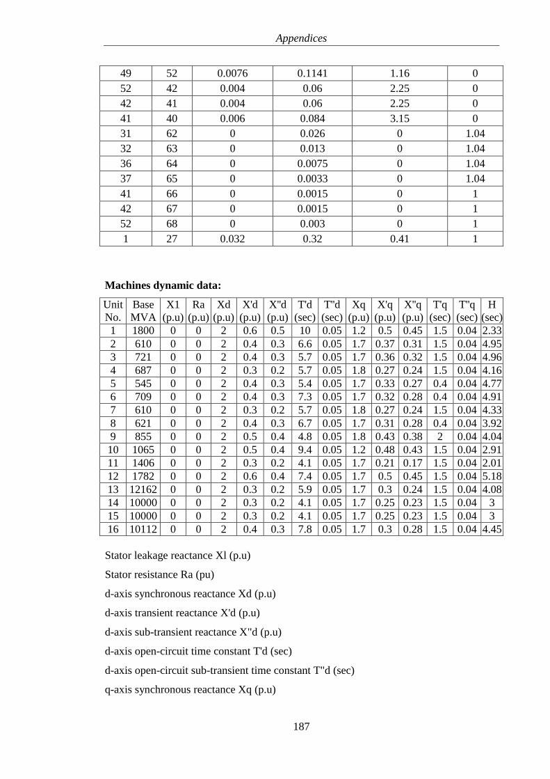
Appendices
187
49 52 0.0076 0.1141 1.16 0
52 42 0.004 0.06 2.25 0
42 41 0.004 0.06 2.25 0
41 40 0.006 0.084 3.15 0
31 62 0 0.026 0 1.04
32 63 0 0.013 0 1.04
36 64 0 0.0075 0 1.04
37 65 0 0.0033 0 1.04
41 66 0 0.0015 0 1
42 67 0 0.0015 0 1
52 68 0 0.003 0 1
1 27 0.032 0.32 0.41 1
Machines dynamic data:
Unit
No.
Base
MVA
X1
(p.u)
Ra
(p.u)
Xd
(p.u)
X'd
(p.u)
X''d
(p.u)
T'd
(sec)
T''d
(sec)
Xq
(p.u)
X'q
(p.u)
X''q
(p.u)
T'q
(sec)
T''q
(sec)
H
(sec)
1 1800 0 0 2 0.6 0.5 10 0.05 1.2 0.5 0.45 1.5 0.04 2.33
2 610 0 0 2 0.4 0.3 6.6 0.05 1.7 0.37 0.31 1.5 0.04 4.95
3 721 0 0 2 0.4 0.3 5.7 0.05 1.7 0.36 0.32 1.5 0.04 4.96
4 687 0 0 2 0.3 0.2 5.7 0.05 1.8 0.27 0.24 1.5 0.04 4.16
5 545 0 0 2 0.4 0.3 5.4 0.05 1.7 0.33 0.27 0.4 0.04 4.77
6 709 0 0 2 0.4 0.3 7.3 0.05 1.7 0.32 0.28 0.4 0.04 4.91
7 610 0 0 2 0.3 0.2 5.7 0.05 1.8 0.27 0.24 1.5 0.04 4.33
8 621 0 0 2 0.4 0.3 6.7 0.05 1.7 0.31 0.28 0.4 0.04 3.92
9 855 0 0 2 0.5 0.4 4.8 0.05 1.8 0.43 0.38 2 0.04 4.04
10 1065 0 0 2 0.5 0.4 9.4 0.05 1.2 0.48 0.43 1.5 0.04 2.91
11 1406 0 0 2 0.3 0.2 4.1 0.05 1.7 0.21 0.17 1.5 0.04 2.01
12 1782 0 0 2 0.6 0.4 7.4 0.05 1.7 0.5 0.45 1.5 0.04 5.18
13 12162 0 0 2 0.3 0.2 5.9 0.05 1.7 0.3 0.24 1.5 0.04 4.08
14 10000 0 0 2 0.3 0.2 4.1 0.05 1.7 0.25 0.23 1.5 0.04 3
15 10000 0 0 2 0.3 0.2 4.1 0.05 1.7 0.25 0.23 1.5 0.04 3
16 10112 0 0 2 0.4 0.3 7.8 0.05 1.7 0.3 0.28 1.5 0.04 4.45
Stator leakage reactance Xl (p.u)
Stator resistance Ra (pu)
d-axis synchronous reactance Xd (p.u)
d-axis transient reactance X'd (p.u)
d-axis sub-transient reactance X"d (p.u)
d-axis open-circuit time constant T'd (sec)
d-axis open-circuit sub-transient time constant T"d (sec)
q-axis synchronous reactance Xq (p.u)

Appendices
188
q-axis transient reactance X'q (p.u)
q-axis sub-transient reactance X"q (p.u)
q-axis open-circuit time constant T'q (sec)
q-axis open circuit sub-transient time constant T"q (sec)
Inertia constant H (sec)
Exciter System Data:
Machine
No.
Tr
(sec)
Ka
(pu)
Ta
(sec)
Tb
(sec)
Tc
(sec)
Vrmax
(pu)
Vrmin
(pu)
1 0 100 0.05 0 0 5 -5
2 0 100 0.05 0 0 5 -5
3 0 100 0.05 0 0 5 -5
4 0 100 0.05 0 0 5 -5
5 0 100 0.05 0 0 5 -5
6 0 100 0.05 0 0 5 -5
7 0 100 0.05 0 0 5 -5
8 0 100 0.05 0 0 5 -5
9 0 100 0.05 0 0 5 -5
10 0 100 0.05 0 0 5 -5
11 0 100 0.05 0 0 5 -5
12 0 100 0.05 0 0 5 -5
13 0 100 0.05 0 0 5 -5
14 0 100 0.05 0 0 5 -5
15 0 100 0.05 0 0 5 -5
16 0 100 0.05 0 0 5 -5
b
c
sT
sT
1
1
rsT1
1
a
a
sT
K
1
TV
refV maxRV
minRV
fdE
External Input
Block diagram of the exciter model
Transducer filter time constant Tr (sec)
Voltage regulator gain Ka (p.u)
Voltage regulator time constant Ta (sec)
Transient gain reduction time constant Tb (sec)
Transient gain reduction time constant Tc (sec)
Maximum voltage regulator output Vrmax (p.u)
Minimum voltage regulator output Vrmin (p.u)

Appendices
189
Speed governors’ data:
Machine
number
wf
(pu)
1/R
(pu)
Tmax
(sec)
Ts
(sec)
Tc
(sec)
T3
(sec)
T4
(sec)
T5
(sec)
1 1 25 1 0.1 0.5 0 1.25 5
2 1 25 1 0.1 0.5 0 1.25 5
3 1 25 1 0.1 0.5 0 1.25 5
4 1 25 1 0.1 0.5 0 1.25 5
5 1 25 1 0.1 0.5 0 1.25 5
6 1 25 1 0.1 0.5 0 1.25 5
7 1 25 1 0.1 0.5 0 1.25 5
8 1 25 1 0.1 0.5 0 1.25 5
9 1 25 1 0.1 0.5 0 1.25 5
10 1 25 1 0.1 0.5 0 1.25 5
11 1 25 1 0.1 0.5 0 1.25 5
12 1 25 1 0.1 0.5 0 1.25 5
13 1 25 1 0.1 0.5 0 1.25 5
14 1 25 1 0.1 0.5 0 1.25 5
15 1 25 1 0.1 0.5 0 1.25 5
16 1 25 1 0.1 0.5 0 1.25 5
R
1
ssT1
1
csT
sT
1
1 3
5
4
1
1
sT
sT
maxT
minT
refP
purrT
0.1
Block diagram of the turbine speed governor
Speed set point ωf (p.u)
Steady state gain 1/R (p.u)
Maximum power order Tmax (p.u) on generator base
Servo time constant Ts (sec)
Governor time constant Tc (sec)
Transient gain time constant T3 (sec)
HP section time constant T4 (sec)
Reheater time constant T5 (sec)

Appendices
190
Appendix A2: Data of the 10 machines-39-bus IEEE test system
Line data:
From Bus To Bus Resistance Reactance Susceptance
1 2 0.0035 0.0411 0.6987
1 39 0.001 0.025 0.75
2 3 0.0013 0.0151 0.2572
2 25 0.007 0.0086 0.146
3 4 0.0013 0.0213 0.2214
3 18 0.0011 0.0133 0.2138
4 5 0.0008 0.0128 0.1342
4 14 0.0008 0.0129 0.1382
5 6 0.0002 0.0026 0.0434
5 8 0.0008 0.0112 0.1476
6 7 0.0006 0.0092 0.113
6 11 0.0007 0.0082 0.1389
7 8 0.0004 0.0046 0.078
8 9 0.0023 0.0363 0.3804
9 39 0.001 0.025 1.2
10 11 0.0004 0.0043 0.0729
10 13 0.0004 0.0043 0.0729
13 14 0.0009 0.0101 0.1723
14 15 0.0018 0.0217 0.366
15 16 0.0009 0.0094 0.171
16 17 0.0007 0.0089 0.1342
16 19 0.0016 0.0195 0.304
16 21 0.0008 0.0135 0.2548
16 24 0.0003 0.0059 0.068
17 18 0.0007 0.0082 0.1319
17 27 0.0013 0.0173 0.3216
21 22 0.0008 0.014 0.2565
22 23 0.0006 0.0096 0.1846
23 24 0.0022 0.035 0.361
25 26 0.0032 0.0323 0.513
26 27 0.0014 0.0147 0.2396
26 28 0.0043 0.0474 0.7802
26 29 0.0057 0.0625 1.029
28 29 0.0014 0.0151 0.249
12 11 0.0016 0.0435 0.0000
12 13 0.0016 0.0435 0.0000
6 31 0.0000 0.0250 0.0000
10 32 0.0000 0.0200 0.0000
19 33 0.0007 0.0142 0.0000
20 34 0.0009 0.0180 0.0000
22 35 0.0000 0.0143 0.0000
23 36 0.0005 0.0272 0.0000
25 37 0.0006 0.0232 0.0000

Appendices
191
2 30 0.0000 0.0181 0.0000
29 38 0.0008 0.0156 0.0000
19 20 0.0007 0.0138 0.0000
Machines data:
Unit
No. H Ra x'd x'q xd xq T'do T'qo xl
1 500 0 0.006 0.008 0.02 0.019 7.0 0.7 0.003
2 30.3 0 0.0697 0.17 0.295 0.282 6.56 1.5 0.035
3 35.8 0 0.0531 0.0876 0.2495 0.237 5.7 1.5 0.0304
4 28.6 0 0.0436 0.166 0.262 0.258 5.69 1.5 0.0295
5 26.0 0 0.132 0.166 0.67 0.62 5.4 0.44 0.054
6 34.8 0 0.05 0.0814 0.254 0.241 7.3 0.4 0.0224
7 26.4 0 0.049 0.186 0.295 0.292 5.66 1.5 0.0322
8 24.3 0 0.057 0.0911 0.29 0.28 6.7 0.41 0.028
9 34.5 0 0.057 0.0587 0.2106 0.205 4.79 1.96 0.0298
10 42 0 0.031 0.008 0.1 0.069 10.2 0 0.0125
Exciter System Data:
Unit
No. TR KA TA TB TC Vsetpoint EfdMax EfdMin
1 0.01 200 0.015 10 1 1.03 5 -5
2 0.01 200 0.015 10 1 0.982 5 -5
3 0.01 200 0.015 10 1 0.9831 5 -5
4 0.01 200 0.015 10 1 0.9972 5 -5
5 0.01 200 0.015 10 1 1.0123 5 -5
6 0.01 200 0.015 10 1 1.0493 5 -5
7 0.01 200 0.015 10 1 1.0635 5 -5
8 0.01 200 0.015 10 1 1.0278 5 -5
9 0.01 200 0.015 10 1 1.0265 5 -5
10 0.01 200 0.015 10 1 1.0475 5 -5
Speed governors’ data:
Machine
number
wf
(pu)
1/R
(pu)
Tmax
(sec)
Ts
(sec)
Tc
(sec)
T3
(sec)
T4
(sec)
T5
(sec)
1 1 200 1 0.1 0.5 0 1.25 5
2 1 200 1 0.1 0.5 0 1.25 5
3 1 200 1 0.1 0.5 0 1.25 5
4 1 200 1 0.1 0.5 0 1.25 5
5 1 200 1 0.1 0.5 0 1.25 5
6 1 200 1 0.1 0.5 0 1.25 5
7 1 200 1 0.1 0.5 0 1.25 5
8 1 200 1 0.1 0.5 0 1.25 5
9 1 200 1 0.1 0.5 0 1.25 5
10 1 200 1 0.1 0.5 0 1.25 5
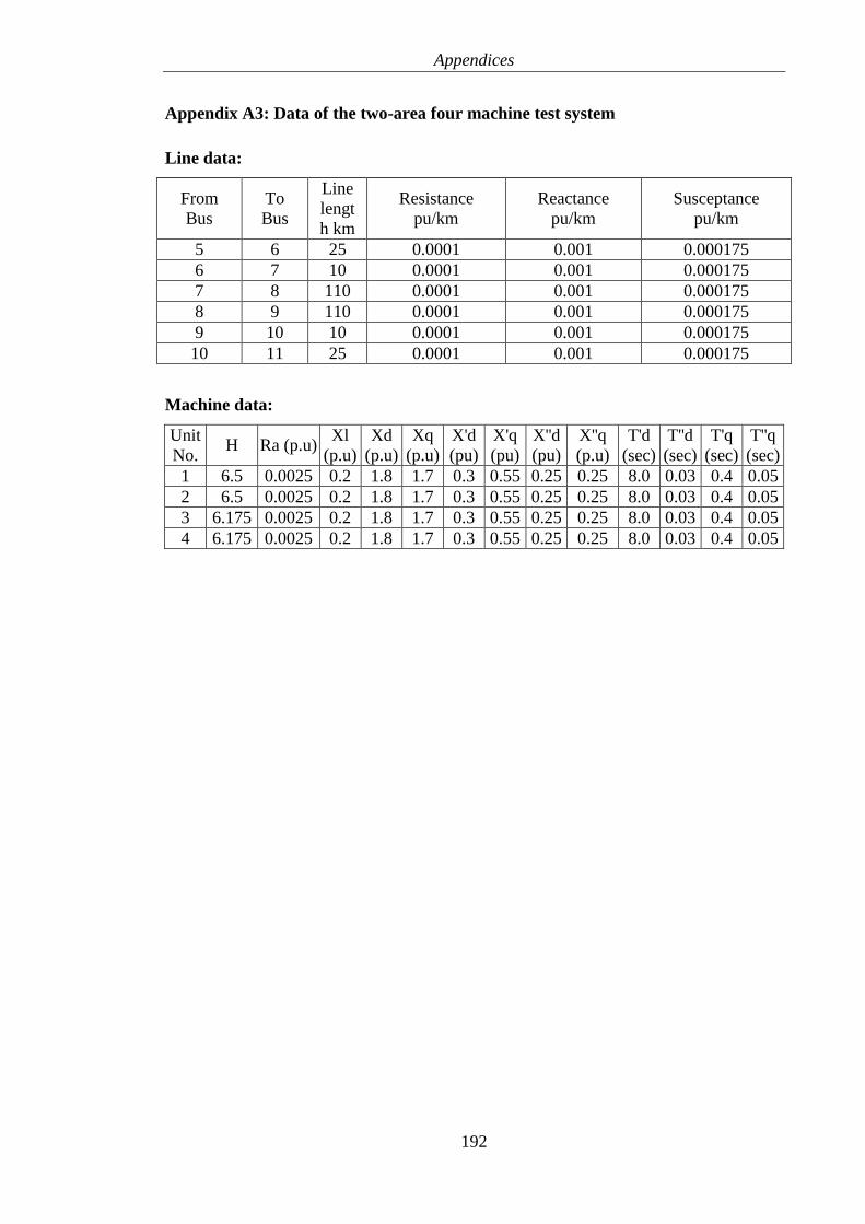
Appendices
192
Appendix A3: Data of the two-area four machine test system
Line data:
From
Bus
To
Bus
Line
lengt
h km
Resistance
pu/km
Reactance
pu/km
Susceptance
pu/km
5 6 25 0.0001 0.001 0.000175
6 7 10 0.0001 0.001 0.000175
7 8 110 0.0001 0.001 0.000175
8 9 110 0.0001 0.001 0.000175
9 10 10 0.0001 0.001 0.000175
10 11 25 0.0001 0.001 0.000175
Machine data:
Unit
No. H Ra (p.u)
Xl
(p.u)
Xd
(p.u)
Xq
(p.u)
X'd
(pu)
X'q
(pu)
X''d
(pu)
X''q
(p.u)
T'd
(sec)
T''d
(sec)
T'q
(sec)
T''q
(sec)
1 6.5 0.0025 0.2 1.8 1.7 0.3 0.55 0.25 0.25 8.0 0.03 0.4 0.05
2 6.5 0.0025 0.2 1.8 1.7 0.3 0.55 0.25 0.25 8.0 0.03 0.4 0.05
3 6.175 0.0025 0.2 1.8 1.7 0.3 0.55 0.25 0.25 8.0 0.03 0.4 0.05
4 6.175 0.0025 0.2 1.8 1.7 0.3 0.55 0.25 0.25 8.0 0.03 0.4 0.05

Appendices
193
Appendix A4: Related Publications
1. Alsafih, H.A.; Dunn, R.; , "Determination of coherent clusters in a multi-machine
power system based on wide-area signal measurements," Power and Energy Society
General Meeting, 2010 IEEE , vol., no., pp.1-8, 25-29 July 2010
2. Alsafih, H.A.; Dunn, R.W.; , "Identification of critical areas for potential wide- area
based control in complex power systems based on coherent clusters," Universities
Power Engineering Conference (UPEC), 2010 45th International , vol., no., pp.1-6,
Aug. 31 2010-Sept. 3 2010
3. Alsafih, H. A.; Dunn, R. W.; , "Performance of Wide-Area based Fuzzy Logic
Power System Stabilizer," Universities' Power Engineering Conference (UPEC),
Proceedings of 2011 46th International , vol., no., pp.1-6, 5-8 Sept. 2011
![27 november 2013 [Lezing: Rechtszekerheid van NEN 1010] Spreker: Bart Wams Rechtszekerheid van NEN 1010 Door: Bart Wams](https://img.dokumen.tips/doc/110x75/5551a0ed4979591f3c8b642e/27-november-2013-lezing-rechtszekerheid-van-nen-1010-spreker-bart-wams-rechtszekerheid-van-nen-1010-door-bart-wams.jpg)