Supporting Information for “Translocation

intermediates of Ubiquitin through an

α-Hemolysin nanopore: implications for detection

of post-translational modifications”

Emma Letizia Bonome†, Fabio Cecconi‡, and Mauro Chinappi‖

E-mail:

†Dipartimento di Ingegneria Meccanica e Aerospaziale, Sapienza Universita di Roma, Via

Eudossiana 18, 00184, Roma, Italia.

‡ CNR-Istituto dei Sistemi Complessi UoS Sapienza, Roma, 00185, Italia.

‖Dipartimento di Ingegneria Industriale, Universita di Roma Tor Vergata, Roma, 00133,

Italia.

E-mail: mauro.chinappi@uniroma2.it

1

Electronic Supplementary Material (ESI) for Nanoscale.This journal is © The Royal Society of Chemistry 2019

Table S1: List of the simulations performed for the C- and N-pulling cases. The first columnreports the simulation code TFSx where T is the pulling terminus (C or N), F the code forthe forcing (F1 = 0.75 nN, F2 = 0.65 nN and F3 = 0.6nN, S is the starting conformation(native conformation Ω or a pre-unfolded conformation Υ), and x (1 . . . 5) indicates thereplica number. The second column reports the translocation time. If the Ubq does notcompletely translocate during the simulation, the second column reports the symbol “−”and the total simulation time Tw is indicated in parenthesis. The third column reports thestalls observed along the trajectory.

Simulation Translocation time (ns) Stalls

C1Ω1 14.2 I II III IV VC1Ω2 18.3 I II III IV VC1Ω3 17.5 I II III IV VC1Ω4 – (28) I II III IV VC1Ω5 18.5 I II III IV VC2Ω1 – (50) I II III IV V

C2Υ1 33.7 I II III IV VC2Υ2 30.9 I II III IV VC2Υ3 29.2 I II III IV VC2Υ4 28.3 I II III IV VC2Υ5 28.5 I II III IV VC3Υ1 – (44) I II III IV VC3Υ2 – (44) I II III IV VC3Υ3 38.5 I II III IV VC3Υ4 43.4 I II III IV VC3Υ5 – (44) I II III IV V

N1Ω1 29.4 I II IIIN1Ω2 33.24 I II IIIN1Ω3 46.44 I II IIIN1Ω4 – (48) I II IIIN1Ω5 22.68 I II IIIN2Ω1 – (40) I II III

N2Υ1 42 I II IIIN2Υ2 42 I II IIIN2Υ3 23.9 I II IIIN2Υ4 21.3 I II IIIN2Υ5 28.4 I II III

2

-0.4

0

0.4

0.8

1.2

1.6

0 2 4 6 8 10 12 14

F [n

N]

t [ns]

Figure S1: Constant velocity steered molecular dynamics (cvSMD) for C-terminus pulling.Time evolution of the z−component of Fv. The force profile shows distinct peaks corre-sponding to specific unfolding of secondary structure elements, e.g., β5 at 2 ns, β4 and β3at 3 ns, HA at 6.5 ns. The horizontal blue dashed lines correspond to the selected values ofthe force at which we run the cfSMD simulations, F1 = 0.75 nN, F2 = 0.65 nN and F3 = 0.6nN.

3

1 MET P

4 PHE P

7 THR P

10 GLY P

13 ILE P

16 GLU P

19 PRO P

22 THR P

25 ASN P

28 ALA P

31 GLN P

34 GLU P

37 PRO P

40 GLN P

43 LEU P

46 ALA P

49 GLN P

52 ASP P

55 THR P

58 ASP P

61 ILE P

64 GLU P

67 LEU P

70 VAL P

73 LEU P

76 GLY P

HelixTurnExtended conformationIsolated bridge3-10 helix

5 ns 10 ns 15 ns0 ns

Figure S2: Time evolution of secondary structure elements for the C-terminus simulationC2Ω1 applied force F2 = 0.65 nN (figure 2A of the manuscript). The color key and the one-letter structure code is the one used by the STRIDE software1. The analysis is performedusing VMD2. Color-code: yellow corresponds to “Extended conformation”, i.e. the maincomponent of beta sheets; aqua corresponds to “Turn”, another beta sheet component, blueand pink correspond to 3− 10 and α helices, respectively, green to the isolated bridge whilewhite stands for random coil, i.e. no secondary structure.

4

z C [Å

]

IV

A)

D)

C)

E)

B)

*

I

II

αHL

αHL

αHL

αHL

αHL

-300

-150

0

150C1Ω1

III

-300

-150

0

150C1Ω2

IV

-300

-150

0

150C1Ω3

I

IV

-300

-150

0

150C1Ω4

I

I

IV

III

III

-300

-150

0

150C1Ω5

I

Figure S3: Constant force steered Molecular Dynamics Simulation (cfSMD) for C-terminuspulling. A-E) Time evolution of C-terminus z−coordinate for simulation starting from thenative conformation Ω, pulling force F1 = 0.75 nN. Simulations C1Ω1, C1Ω2, C1Ω3, C1Ω5

complete the translocation in a time window Tw < 20 ns, while in the C1Ω4 the protein getstuck in the pore in a conformation, identified with ∗ similar to the stall IV reported in figure2F of the paper. The translocation intermediates corresponding to the stalls are indicatedusing the roman numerals. Stalls I and III are present in several simulations, while the stallII appears only in one of them. As discussed in the paper, a possible explanation is that,while stall I and III stalls correspond to rearrangements of the native secondary structurestall II is associated to a contingent interaction of the unfolded residues originally belongingto β4 and β5 (residue 48-49, 66-71) with the interior pore surface. Consequently, we expectthat, stall I and III are quite reproducible among the replicas while stall II not.

5

I

III

A) B)

-120

-100

-80

-60

-40

-20

0

20

40

60

0 1 2 3 4 5 6 7 8 9

z C[ Å

]

time [nS]

C1Ω2

Figure S4: Υ conformation for C-terminus. A) Time evolution of C-terminus z−coordinatefor a simulation starting from native structure, pulling force F1 = 0.75 nN. From this translo-cation pathway we have selected a conformation after stall III, red rectangle at zC ' −80 A,t ' 6.5 ns. This conformation, indicated as Υ, is used as initial condition for two new setsof simulations C2Υx and C3Υx, x = 1 . . . 5, performed to explore the whole translocationpathway.

6

z C [Å

]

IV

A)

D)

C)

E)

B)

V

V

IV

IV

IV

-300

-150

0C2Υ1

-300

-150

0C2Υ2

-300

-150

0C2Υ3

-300

-150

0C2Υ4

-300

-150

0C2Υ5

V

V

IV

Figure S5: Constant force steered Molecular Dynamics Simulation (cfSMD) for C-terminuspulling. A-E) Time evolution of C-terminus z−coordinate for simulation starting from con-formation Υ, pulling force F2 = 0.65 nN.

7

z C [Å

]

A)

D)

C)

E)

B)

V

IV

IV

-300

-150

0C3Υ1

-300

-150

0C3Υ2

-300

-150

0C3Υ3

-300

-150

0C3Υ4

IV

-300

-150

0C3Υ5

V

V

V

*

III

Figure S6: Constant force steered Molecular Dynamics Simulation (cfSMD) for C-terminuspulling. A-E) Time evolution of C-terminus z−coordinate for simulation starting from con-formation Υ, pulling force F3 = 0.60 nN. The simulations C3Υ1, C3Υ2, C3Υ5 do not com-plete the translocation and the protein remains blocked in the nanopore in the intermediateV reported in the figure 2 of the paper. The time window is Tw = 44 ns (only the first 30ns are shown). The simulation C3Υ4 presents the same stall ∗ previously analyzed in thefigure S3D where the two βstrands, β2 and β1, get stuck at the cis entrance and unfoldbefore entering the vestibule.

8

-300

-150

0

150 N1Ω3

-300

-150

0

150N1Ω5

-300

-150

0

150 N1Ω1

z N [Å

]

I

A)

D)

C)

E)

B)

-300

-150

0

150 N1Ω2

III

0

II

0

0

0

I

I

II

II

II

*

αHL

αHL

αHL

αHL

*

-300

-150

0

150 N1Ω4

αHLI

*

III

III

0

Figure S7: Constant force steered Molecular Dynamics Simulation (cfSMD) for N-terminuspulling. A-E) Time evolution of N-terminus z−coordinate for simulation N1Ωx, x ∈ (1, 5),i.e. simulation pulled from native initial condition and force F1 = 0.75 nN. SimulationsN1Ω1, N1Ω2, N1Ω3, N1Ω5 complete the translocation in a time window Tw = 50 ns, whilein the N1Ω4 the protein get stuck in the pore in a conformation, identified with ∗ similarto the stall II reported in figure 3 on the paper. All the simulations show the same translo-cation intermediates already reported in the figure 3 of the paper. Also a first stall (0) isapparent. In this conformation, all the secondary structure elements are still folded althoughthe tertiary structure is slightly deformed and the protein get stuck at the cis entrance.

9

I

II

A) B)

-120

-100

-80

-60

-40

-20

0

20

40

60

0 5 10 15 20 25 30 35

z N[ Å

]

time [nS]

N1Ω3

Figure S8: Υ conformation for N-terminus pulling. A) Time evolution of N-terminus forsimulation starting from the native conformation Ω, pulling force F1 = 0.75 nN, simulationcode N1Ω3. From this translocation pathway, we selected a conformation after stall II (redsquare at zN ' −120 A, t ' 31 ns. This conformation, indicated as Υ in the simulationcode, is used as initial condition for a new sets of simulations N2Υx x (1 . . . 5) conceived toexplore the whole the translocation pathway.

10

A)

D)

C)

E)

B)

III

-300

-150

0N2Υ5

III

III

III

II

II

II

II

II

-300

-150

0N2Υ1

-300

-150

0N2Υ2

-300

-150

0N2Υ3

-300

-150

0N2Υ4

Figure S9: Constant force steered Molecular Dynamics Simulation (cfSMD) for N-terminuspulling. A-E) Time evolution of N-terminus z−coordinate starting from conformation Υ.Pulling force F2 = 0.65 nN. All the simulations show the same translocation intermediates,II and III, reported in the figure 3 on the paper.

11

β1 β2 β3 β4 β5

β1

β2

β3

β4

β5

HA HB HC

HA

HB

HC

0 10 20 30 40 50 60 700

10

20

30

40

50

60

70

Figure S10: Heavy-atom contact map generated from the crystallographic structure of theubiquitin, pdb entry 1UBQ5. A cutoff of Rc = 5 A selects M = 190 native contacts for1UBQ structure.

S1. Go-model with heavy map: C-pulling

The Ubq is modelled by a Go-like force field proposed by Clementi et al.3. The details about

force-field parameterization and implementation can be found in3,4. The chain is represented

by taking into account only Cα atom positions (beads), since we are mainly interested in

the structural rearrangements of the backbone along the translocation pathway. We recall

that Go-models are such that energy function takes its minimum on the coordinates of

the crystallographic structure of the native state, in the present work such coordinates are

extracted from the pdb entry 1UBQ5. A simple way to achieve that the native structure

is a minimum of the potential energy is by introducing the notion of native interactions,

or contacts. In this work, we consider two residues i, j in native interaction if they share a

couple of heavy-atoms, i.e. all atoms but Hydrogens and Nitrogens, within a cutoff distance

Rc < 5 A. The resulting contact map is reported in Fig. S10, showing the 190 contacts.

The interactions between the beads are associated to peptide bonds, angular bending,

torsional deformation and native contacts, see3,4, leading to the energy function for a N

12

residue protein

ΦGo =N−1∑i=1

Vp(ri,i+1) +N−2∑i=1

Vθ(θi − θ0i ) +

N−3∑i=1

Vϕ(ϕi − ϕ0i )

+∑

i,j≥i+3

Vnb(rij). (1)

The peptide bond term, Vp, enforcing the chain connectivity, is a stiff harmonic potential

allowing only small oscillations of the bond lengths around their crystallographic values.

Likewise, the bending potential Vθ allows only small fluctuations of the bending angles θi

around their native values θ0i . Dihedral potential Vφ (associated to torsional deformation)

further contributes to the correct formation of the native secondary structure characterized

also by angles ϕ0i . Finally, the long-range potential Vnb, which favors the formation of the cor-

rect native tertiary structure, is a collection of two-body 12-10 Lennard-Jones contributions

that are attractive between residues forming native contacts and repelling for non-native

couples.

S1.1. Pore geometry

The confining effect of the αHL nanopore is described by the following potential acting only

in the pore region, 0 < x < L,

Vp(x, y, z) = V0

0 y2 + z2 ≤ R2(x)

[(y

R(x)

)2

+

(z

R(x)

)2

− 1

]my2 + z2 > R2(x) .

(2)

To fit the vestibule-barrel shape of the αHL, the pore radius is modulated as

R(x) =Rv +Rb

2− Rv −Rb

2tanh[α(x− xc)] (3)

13

0.1250.25

0.51248

163264

128

0 10 20 30 40 50 60 70

Resi

denc

e tim

e

Ncis

0.1250.25

0.51248

163264

128

0 10 20 30 40 50 60 70

A) B)

Figure S11: A) Sketch of the coarse grained simulation set-up. B) Histogram of the residencetime for the variable Ncis obtained averaging over 2000 C-pulling runs starting from nativeconformation for pulling force F = 1.6. The large peak is associated to the unfolding of β5.

with L ' 100 A, Rv = 10 A (for the vestibule), Rb = 4 A (for the barrel), xc = L/2 and

m = 4.

A repulsive force, Fw(x), orthogonal to planes x = 0, x = L and vanishing for y2 + z2 <

R(x)2, models the presence of the impenetrable membrane hosting the pore

Fw(x) =

− eλx

x+ cx ≤ 0

0 0 < x < L

e−λ(x−L)

x− L+ cx ≥ L

(4)

with c = 10−4 A being a regularisation cutoff to avoid numerical overflow and λ = 6 A−1.

S1.2. Simulation protocol

The importing mechanism that drives the protein into the pore is simplified to a constant

pulling force (F, 0, 0) acting only on the C-terminus bead (r76). Moreover, the pulled terminus

is constrained to slide along the pore axis for all time, i.e., y76(t) = z76(t) = 0. Simulations

14

were performed by using a coarse grained molecular dynamics at constant temperature T =

0.8 implemented with a Langevin dynamics that evolves the position ri of the i = 1, . . . , N

residues

Maari = −γri −∇ri (ΦGo + Vp) + F76 + Fw(xi) + Zi , (5)

where Maa denotes the average amino acid mass, Zi is a random force with zero average and

correlation 〈Zi,µ(0)Zi,ν(t)〉 = 2γkBTδµ,νδ(t), with µ, ν = x, y, z and kB being the Boltzmann’s

constant (kB = 1), F76 the importing force and ΦGo, Vp and Fw given by (1), (2) and (4),

respectively. We used γ = 5.0 and a time step h = 0.005. Each translocation run started by

positioning the native structure with the C-terminus at x76 = (10, 0, 0) A and thermalizing

for teq = 104 time steps with the C-terminal blocked. Then, the forcing is turned on and the

simulation is stopped when all the residues reached the trans side (xi > L). Like in the all-

atom case, the unfolding of the first translocation intermediate requires a quite large force,

hence, once unfolded, the remaining translocation intermediates are less evident. Therefore,

we employed an approach similar to the one described for all-atom MD. First, we performed

high force runs (F76 = 2.2) to explore the complete translocation pathway. Then, we selected

a conformation just after the unfolding of the first structural cluster (e.g. after stall III) and,

thus, we used it as starting conformation for runs at lower force (F76 = 1.6).

To characterize the dynamics of the translocation we measure the time course of the two

collective variables

Ncis(t) = N −N∑

i=1

Θ(xi) , (6)

and

Ncis,v(t) = N −N∑

i=1

Θ(xi − L/2) , (7)

Θ(s) is the unitary step function. Ncis and Ncis,v correspond to the number of residues that

have not yet entered the pore vestibule (Ncis) and the barrel (Ncis,v), respectively. In essence,

at the initial condition Ncis = Ncis,v = 76, i.e. all the 76 amino acids are outside the pore

at the cis side. As long as the translocation proceeds, both variables decrease. Peaks in the

15

histogram of these variables indicate the presence of translocation bottlenecks.

S2. Electrolyte accessibility estimator

In experiments, nanopore clogging is usually characterized in term of the current blockade

(I0 − I(t))/I0 or, in alternative, in term of the residual current I(t)/I0, where I(t) is the

current trace associated to the nanopore-molecule interaction and I0 is the open pore current.

The residual current I(t)/I0 can be written in term of pore resistances, indeed, using Ohm’s

law,

Ires(t) =I(t)

I0

=R0

R(t). (8)

In a quasi-1D continuum model, the resistance of a pore can be modelled as

R =

∫ L

0

ρ(z)

A(z)dz , (9)

where the z−axis coincides with the pore axis, the pore goes from z = 0 to z = L, ρ(z) is

the electrolyte resistivity, here assumed to be homogeneous, and A(z) is the area of the pore

section available to the electrolyte passage. Access resistances are neglected in expression (9).

The integral in eq. (9) can be approximated dividing the system in Nz slabs of size ∆z

obtaining

R =Nz∑i=1

ρ

Ai

∆z , (10)

while the available effective area Ai can be estimated as Ai = Vi/∆z where Vi is the volume

occupied by the electrolyte in the i-th slab.

Inspired by these continuum quasi-1D arguments, we defined the electrolyte accessibility

estimator as

c(t) =R0

R(t). (11)

16

In particular, we calculated eq. (10) for each frame and then, we used this value in eq. (11).

The volume Vi appearing in eq. (10) is estimated as the number of electrolyte molecules

(water or ions) in the i-th slab times a reference volume Vele that corresponds to the typical

volume of a water molecule. Note that, in the expression (11), Vele simplifies, so its exact

value is not relevant for our purposes. The time evolution of c(t) is highly noisy, hence, for

the sake of clarity, in figure 5 of the main text we reported a running average performed over

10 values from consecutive snapshots separated by 0.04 ns.

The above model is based on several hypotheses that are violated by the actual αHL

pore shape. In particular, the continuum assumption is not justified at nanoscale, moreover,

the model implicitly assumes a smooth variation of Ai along the pore axis (quasi-1D) and

a homogeneous electrolyte resistivity ρ. Nevertheless, although a quantitative agreement

with the residual current is not expected, we are confident that the trend in the current

levels would be the same. In particular, we expect that the smaller current (larger blockade)

would correspond to stall III while stall IV and V would be associated to progressively larger

currents (smaller blockades). As a final comment, for readers reference, it is worth mentioning

that similar quasi-1D models have been employed in other all-atom MD studies6,7.

S3. Structural analysis

To check if there were systematic differences among the translocation intermediates over the

different replicas (e.g. if stall V from simulations C3Υ3 and C3Υ5 differs) we performed a

structural clustering analysis as follows:

1. For a given stall, we selected all the corresponding MD frames for all the simulations

where the stall appears.

2. For each frame, we selected only the folded portion of the Ubq. For instance, in the

case of stall III for C-pulling, we selected the residues from 1 to 35, corresponding to

17

the HA, β1 and β2. Hence, at this stage, we have a set of N structures corresponding

to a given stall.

3. We then calculated the RMSD distance among all the N structures obtaining an N×N

distance matrix.

4. The distance matrix was used as input of a clustering algorithm (complete linkage

method for hierarchical clustering from cluster library8 in the R software9)

5. As usual in clustering analysis, we calculated the average silhouette for different par-

titions of the data (number of clusters).

For all the stalls, we get a low silhouette (maximum value ' 0.35), hence, indicating no clear

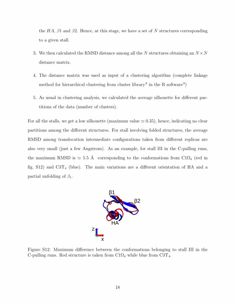
partitions among the different structures. For stall involving folded structures, the average

RMSD among translocation intermediate configurations taken from different replicas are

also very small (just a few Angstrom). As an example, for stall III in the C-pulling runs,

the maximum RMSD is ' 5.5 A corresponding to the conformations from C1Ω4 (red in

fig. S12) and C3Υ4 (blue). The main variations are a different orientation of HA and a

partial unfolding of β1.

z

x

HA

β2

β1

Figure S12: Maximum difference between the conformations belonging to stall III in theC-pulling runs. Red structure is taken from C1Ω4 while blue from C3Υ4.

18

References

(1) Heinig, M.; Frishman, D. STRIDE: a web server for secondary structure assignment from

known atomic coordinates of proteins. Nucleic acids research 2004, 32, W500–W502.

(2) Humphrey, W.; Dalke, A.; Schulten, K. VMD: visual molecular dynamics. 1996, 14,

33–38.

(3) Clementi, C.; Nymeyer, H.; Onuchic, J. N. Topological and energetic factors: what deter-

mines the structural details of the transition state ensemble and en-route intermediates

for protein folding? an investigation for small globular proteins1. Journal of molecular

biology 2000, 298, 937–953.

(4) Cecconi, F.; Guardiani, C.; Livi, R. Testing simplified proteins models of the hPin1 WW

domain. Biophysical journal 2006, 91, 694–704.

(5) Vijay-Kumar, S.; Bugg, C. E.; Cook, W. J. Structure of ubiquitin refined at 1.8

Aresolution. Journal of molecular biology 1987, 194, 531–544.

(6) Si, W.; Aksimentiev, A. Nanopore sensing of protein folding. ACS nano 2017, 11, 7091–

7100.

(7) Di Muccio, G.; Rossini, A. E.; Di Marino, D.; Zollo, G.; Chinappi, M. Insights into

protein sequencing with an α-Hemolysin nanopore by atomistic simulations. Scientific

Reports 2019,

(8) Maechler, M.; Rousseeuw, P.; Struyf, A.; Hubert, M.; Hornik, K. cluster: Cluster Anal-

ysis Basics and Extensions. 2018.

(9) R Core Team, R: A Language and Environment for Statistical Computing. R Foundation

for Statistical Computing: Vienna, Austria, 2015.

19