Transition to turbulence in Hunt's flow in a moderate magnetic field Braiden, LA, Krasnov, D, Molokov, S, Boeck, T & Buhler, L Author post-print (accepted) deposited by Coventry University’s Repository Original citation & hyperlink:

Braiden, LA, Krasnov, D, Molokov, S, Boeck, T & Buhler, L 2016, 'Transition to turbulence in Hunt's flow in a moderate magnetic field' EPL, vol 115, no. 4, 44002 https://dx.doi.org/10.1209/0295-5075/115/44002

DOI 10.1209/0295-5075/115/44002 ISSN 0295-5075 ESSN 1286-4854 Publisher: European Physical Society Copyright © and Moral Rights are retained by the author(s) and/ or other copyright owners. A copy can be downloaded for personal non-commercial research or study, without prior permission or charge. This item cannot be reproduced or quoted extensively from without first obtaining permission in writing from the copyright holder(s). The content must not be changed in any way or sold commercially in any format or medium without the formal permission of the copyright holders. This document is the author’s post-print version, incorporating any revisions agreed during the peer-review process. Some differences between the published version and this version may remain and you are advised to consult the published version if you wish to cite from it.

epl draft

Transition to turbulence in Hunt’s flow in a moderate magneticfield

L. Braiden1, D. Krasnov2, S. Molokov1, T. Boeck2 and L. Buhler3

1 School of Computing, Electronics and Mathematics, Coventry University, Priory Street, Coventry CV1 5FB, UK2 Institute of Thermodynamics and Fluid Mechanics, Technische Universitat Ilmenau, 98684 Ilmenau, Germany3 Institut fur Kern- und Energietechnik, Karlsruher Institut fur Technologie, 76021 Karlsruhe, Germany

PACS 47.35.Tv – Magnetohydrodynamics in fluidsPACS 47.27.Cn – Transition to turbulencePACS 47.27.N- – Turbulent flows, wall-bounded

Abstract – Pressure-driven magnetohydrodynamic duct flow in a transverse uniform magneticfield is studied by direct numerical simulation. The electric boundary conditions correspond toHunt’s flow with perfectly insulating walls parallel to the magnetic field (side walls) and perfectlyconducting walls perpendicular to the magnetic field (Hartmann walls). The velocity distributionexhibits strong jets at the side walls, which are susceptible to instability even at low Reynoldsnumbers Re. We explore the onset of time-dependent flow and transition to states with evolvedturbulence for a moderate Hartmann number Ha = 100. At low Re time-dependence appears inthe form of elongated Ting-Walker vortices at the side walls of the duct, which, upon increasingRe, develop into more complex structures with higher energy and then the side-wall jets partiallydetach from the walls. At high values of Re jet detachments disappear and the flow consists oftwo turbulent jets and nearly laminar core. It is also demonstrated that, there is a range of Re,where Hunt’s flow exhibits a pronounced hysteresis behavior, so that different unsteady states canbe observed for the same flow parameters. In this range multiple states may develop and co-exist,depending on the initial conditions.

Introduction. – Magnetohydrodynamic (MHD)1

flows in ducts play a major role in liquid metal blankets2

for thermonuclear fusion reactors serving for cooling of the3

reactor and for breeding tritium [1]. A very important re-4

quirement to these flows is that they should provide suffi-5

cient mixing of the fluid to improve heat and mass transfer6

characteristics, i.e. provide sufficient level of turbulence.7

This, however, may be problematic as the liquid metal8

flow occurs in a high magnetic field of about 5− 10 Tesla.9

This leads to high MHD interaction between the induced10

currents j and the magnetic field B resulting in a strong11

braking Lorentz body force j ×B, which tends to damp12

turbulence.13

More often than not the ducts have thin electrically con-14

ducting walls, which leads to a velocity profile, shown in15

Fig. 1. Here the basic velocity exhibits a flat core, ex-16

ponential Hartmann layers at the walls transverse to the17

magnetic field (the Hartmann walls), and jets at the walls18

parallel to the field (the side walls). Jets appear due to19

induced electric current within the core of the flow. The20

current must turn (either fully or partially) in the direc- 21

tion of the magnetic field at the side walls to complete the 22

loops, which then close through the conducting Hartmann 23

walls (Fig. 1). Once this happens, the resulting force j×B 24

and its braking effect are reduced in the near-wall region, 25

thus allowing the fluid to flow with higher velocity than 26

in the core. The exact ratio of the core to jet velocities 27

and thus between the mass fluxes strongly depends on the 28

electrical conductivities of the Hartmann- and side-walls. 29

In the extreme case of perfectly electrically insulating side 30

walls and perfectly conducting Hartmann walls (known as 31

Hunt’s flow, see a particular case in [2]), practically all the 32

mass flux is carried by the side-wall jets. 33

We will be concerned here with an electrically conduct- 34

ing, incompressible fluid flow in a square duct, driven 35

by a mean pressure gradient, with kinematic viscosity, 36

ν, density, ρ, and electrical conductivity, σ. The flow 37

is subjected to a uniform magnetic field of intensity B 38

applied in the z-direction (x, y, z are Cartesian coordi- 39

nates, as shown in Fig. 1). For a given mean velocity U , 40

p-1

L. Braiden et al.

Fig. 1: Flow geometry of Hunt’s flow in a square duct. Lami-nar velocity distribution with perfectly conducting Hartmann-and perfectly insulating parallel-walls is shown at Ha = 100(blue); also shown are the streamlines of electric current den-sity (brown).

the flow is characterised by three dimensionless parame-41

ters [3]: the Reynolds number, Re = UL/ν, where L is42

half the distance between the walls, the Hartmann num-43

ber Ha = BL(σ/ρν)1/2, the square of which characterises44

the ratio between the Lorentz and viscous forces, and the45

wall conductance ratio c = σwhw/σL, where σw and hw46

are the electrical conductivity and thickness of the wall,47

respectively. Note that c may be different for each wall.48

A family of the exact solutions for MHD flows with jets49

was obtained in [2]. Early experimental results were re-50

viewed in [4], and the main conclusion was that the jets51

were much thicker than the O(Ha−1/2) thickness of the52

jets in the fully developed flow. Linear stability of a flow53

in a duct with c = 0.07 [5] could not account for this54

increase in the thickness as the instability was fully con-55

tained in the parallel side layers. In addition, the Ting and56

Walker (TW) vortices appeared for critical Reynolds num-57

ber Recr ∼ 300, while in the corresponding experiment [6]58

the instabilities appeared at Recr ∼ 3000. For Hunt’s flow59

linear stability analysis was performed by [7], who discov-60

ered a rich variety of perturbations for Ha < 45, while61

for higher Ha the most unstable mode consisted of TW62

vortices. The controvercies between the theory and the63

experiment were resolved in [8], where for Ha = 200 and64

c = 0.5 direct numerical simulation (DNS) of the tran-65

sition to turbulence were performed. First, it was shown66

that, when TW vortices appear, they are so weak that they67

do not affect the mean velocity profile. For Re > 3500 a68

new effect appeared consisting of partial jet detachment69

from the side walls, which indeed led to thicker jets.70

In this letter we will focus on the transition to turbu-71

lence in Hunt’s flow and present various flow structures72

obtained during the transition. Detailed analysis of these73

state will be presented later in a series of journal papers.74

Procedure and parameters. – We consider the75

MHD equations for incompressible fluid in a quasi-static76

form, which is standard for liquid metals (see, e.g., [3,5,8]).77

The governing equations are solved with second-order fi-78

nite differences using our in-house solver [9]. The bound-79

ary conditions are periodic in the streamwise x-direction.80

Time integration is either fully explicit (using the 2nd or-81

der Adams-Bashforth/Backward-differencing scheme) or 82

with the implicit treatment of the viscous terms 1

Re∇2v. 83

The semi-implicit version is beneficial at low-Re, as it 84

helps to maintain large integration time-steps δt without 85

the loss of numerical stability. 86

The simulations have been conducted in a domain size 87

of 8π × 2× 2 and numerical resolution varied from 512× 88

1282 to 1024× 2562 points in, correspondingly, x-, y- and 89

z-directions. The computational grid is clustered in the 90

wall-normal y- and z-directions by applying the coordinate 91

transformation based on the hyperbolic tangent (see, e.g., 92

[9]). Constant time step δt was maintained at 5×10−4...2× 93

10−3 (depending on Re). The typical runtime contributed 94

to 5×105...106 steps (several hundreds of convective units) 95

using 128...1024 cores, depending on the resolution. 96

A series of DNS has been performed at a fixed Hartmann 97

number Ha = 100, representing the case of moderate mag- 98

netic fields, and a broad range of Re, covering regimes from 99

Re = 200 to 10000. A similar approach with fixed Ha 100

was also used in [8]. In various studies on flow transition 101

the most commonly used scenario is to modulate the ini- 102

tially laminar flow by perturbations. These can be either 103

random noise or a combination of specially constructed 104

modes modulated by random noise (one- or two-step sce- 105

nario, e.g., [10]). In either case the transient evolution 106

and the actual thresholds are governed by many parame- 107

ters, such as the amplitude of perturbations, specific spa- 108

tial shape and distribution, optimal wave-numbers, etc. 109

To avoid this ambiguity, two other scenarios of obtain- 110

ing time-dependent MHD solutions have been adopted. 111

First, we have used fully developed non-MHD turbulent 112

flows, precomputed for the closest possible Re, as the ini- 113

tial state. Then the magnetic field is switched on and the 114

simulation is continued further. This method has the ap- 115

peal that fluctuations are created in a natural way. In 116

another procedure the unsteady MHD solution, obtained 117

for a certain Re, is used as the initial state to study evo- 118

lution to a different target Re, which can be either higher 119

or lower than the initial Re. This method has been most 120

extensively used to study the phenomenon of hysteresis. 121

We have employed both ways of changing Re – with small 122

steps and as a single shot to the target value. The onset 123

of new unsteady solutions or transition between different 124

states have been identified by visual analysis of the flow 125

field and by monitoring the kinetic energy of the trans- 126

verse velocity components qt = u2y + u2

z (see, e.g., [11]). 127

To attain a statisticaly sustained (fully developed) state 128

the simulations have typically run for the time from at 129

least 100 to 1000 convective time-units. 130

Results. – 131

Low- and mid-range values of Re. We begin our dis- 132

cussion with the results of simulations at Re = 500 shown 133

in Fig. 2a. This flow state was obtained using turbu- 134

lent non-MHD flow at Re = 1200 (the smallest Re where 135

turbulence can still exist) as an initial condition. One in- 136

teresting observation is that the turbulent energy drops 137

p-2

Instability of Hunt’s flow

by several orders of magnitude as the magnetic field is138

switched on. Basically, the magnetic field rapidly destroys139

turbulence so that the remaining perturbations can be140

viewed as a residual noise. As a minimum is attained,141

the residual fluctuations start to grow and finally evolve142

into a different unsteady regime. This behavior has been143

found in our simulations performed at other values of Re.144

Here we can clearly observe inherently small vortical145

structures located within the side layer region (Fig. 2a146

and insert). The vortices exhibit anisotropy in the vertical147

z-direction, especially pronounced close to the Hartmann148

walls, as illustrated by the isosurfaces of λ2-criterion. Ac-149

cording to [12], negative regions of λ2 identify coherent150

vortical structures (λ2 is the 2nd eigenvalue of the ten-151

sor SikSkj + ΩikΩkj , where Sij and Ωij are the rate of152

strain and vorticity tensors). The structures are comprised153

of clockwise rotating vortices (CW, thinner ones at the154

side walls) and counter clockwise rotating vortices (CCW,155

thicker ones closer to the core). Hereafter the direction of156

vortex rotations is conventionally defined in respect to the157

right-side if viewed along the flow direction (note the sign158

change at the opposite wall). Both CW and CCW vortices159

are organized in a slightly staggered arrangement. These160

are the so-called TW vortices [5], they appear at low-Re161

and are viewed as the 1st unstable solution of Hunt’s flow.162

The TW vortices are very weak, e.g., for this case their163

kinetic energy is about 0.033% of the total kinetic energy164

of the flow (Table 1), so hardly producing any visible im-165

pact on the integral flow charachteristics, such as the wall166

stresses τw or the total friction coefficient Cf .167

Further increase of Re reveals an interesting and rather168

unexpected behavior of the flow. Namely, using this state169

as the initial condition and increasing Re to 1000, we170

have observed that TW vortices very quickly and nearly171

completely disappear during the initial phase of simula-172

tion. However, after about a hundred of convective units173

of temporal evolution, a new type of vortical structrures174

is developed. These new instabilities are much larger,175

both in size and kinetic energy (about 0.1% of the to-176

tal kinetic energy), are elongated in the flow direction and177

tend to dominate about 50...60% of the flow domain (Fig.178

2b). This particular behavior is observed in the range179

1000 ≤ Re ≤ 1300, where these big vortical structures180

have also been repeatedly reproduced in simulations initi-181

ated by non-MHD turbulent states.182

Increasing Re to 1400, we again observe another flow183

regime. New structures develop in the form of additional184

small-scale CW and CCW rotating vortices, which are lo-185

cated within the large instabilities previously observed at186

1000 ≤ Re ≤ 1300, which evolve in this case too. There187

are quite a few remarkable features concerning these struc-188

tures. On the initial inspection, they are very small in size189

and elongated in the vertical z-direction, as demonstrated190

in Fig. 2c and in Table 1. The shape resembles that of191

”pike-teeth”, which are settled in a staggered arrangement192

in respect to the mid-plane symmetry z = 0. Further anal-193

ysis shows that the kinetic energy of these new structures194

is about two times smaller than the previous instabilities 195

at Re ≤ 1300, contributing 0.05% of the total kinetic en- 196

ergy of the flow. However, the specific distribution of the 197

kinetic energy over velocity components changes. Albeit 198

the streamwise component is still dominating, the energy 199

associated with the vertical component increases by a fac- 200

tor of 2, thus producing stronger anisotropy in the vertical 201

direction (e.g., qz/qy in Table 1). Basically, the ”pike- 202

teeth” can be viewed as rather strong (in amplitude) and 203

short (in the vertical length) modes. Once these structures 204

have developed, they remain in the flow throughout the 205

simulation. At higher Re (up to 1550) they develop more 206

rapidly, stretching in the vertical direction, and demon- 207

strate an alternating behavior along the side walls. 208

To check the validity of the results we have conducted 209

additional verifications. First, it has been found that these 210

structures also arise if the simulation is initiated with tur- 211

bulent state. Secondly, to make sure these structures were 212

not a numerical artifact due to an insufficient grid, we 213

have also performed simulations at higher resolution of 214

2048× 3842 points and found them to appear again. 215

The ”pike-teeth” have been observed in a narrow range 216

1400 ≤ Re ≤ 1550, beyond which they are followed by an- 217

other type of instability – jet detachments, discussed in the 218

next section. Given the narrow range of Re and the grad- 219

ually increasing level of kinetic energy, it seems feasible 220

that the ”pike-teeth” may serve a nuclei of detachments. 221

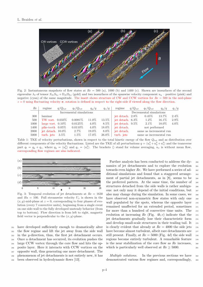
Jet detachments and transition to turbulence. Upon 222

further increase of Re to 1630, we observe that the flow 223

exhibits another time-dependent regime – partial jet de- 224

tachments. The temporal evolution and settlement of this 225

flow regime is shown in Fig. 3 with four phases, corre- 226

sponding to the different times of flow evolution. One can 227

see that at the beginning a very small nuclei of instability 228

– a localized spot – appears at one side wall of the duct 229

(a). As time evolves, this spot grows in size and attains 230

kinetic energy from the mean flow until the side jet visibly 231

detaches from the wall (b). Soon after, the detached struc- 232

ture interacts with the opposite side layer, thus, producing 233

a series of small disturbances (c), which rapidly evolve into 234

similar-sized patterns. Consequently, both walls become 235

populated with detached structures (Fig. 3d). 236

The nature of jet detachments can be understood more 237

thoroughly from the analysis of vortex patterns formed at 238

the side walls, as shown in Fig. 4 for Re = 2000...5000. 239

The plot at Re = 2000 (Fig. 4a) demonstrates small CW 240

rotating vortices, housed at the inner (near wall) region 241

of the domain of the high velocity jet. They are the re- 242

sult of high shearing effects within the inner region of the 243

duct. Simultaneously, CCW vortices are formed between 244

the outer region of the velocity jet and the core flow. Ini- 245

tially, at Re ≤ 1600, the small CCW vortices remain stable 246

travelling in the streamwise direction along with the bulk 247

of the flow. At some point the CCW vortices develop both 248

in size and intensity and have a retarding effect on the jet 249

velocity in the outer region. Eventually the CCW vortices 250

p-3

L. Braiden et al.

Fig. 2: Instantaneous snapshots of flow states at Re = 500 (a), 1000 (b) and 1400 (c). Shown are isosurfaces of the secondeigenvalue λ2 of tensor SikSkj + ΩikΩkj (gold) and two isosurfaces of the spanwise velocity component uy – positive (pink) andnegative (cyan) of the same magnitude. The insert shows structure of CW and CCW vortices for Re = 500 in the mid-planez = 0 using fluctuating velocity v, rotation is defined in respect to the right-side if viewed along the flow direction.

Re regime q/Qtot qt/Qtot qy/q qz/q regime q/Qtot qt/Qtot qy/q qz/q

Incremental simulations Decremental simulations300 laminar jet detach. 2.8% 0.45% 13.7% 2.4%500 TW vort. 0.033% 0.0081% 11.0% 13.5% jet detach. 6.3% 1.2% 16.1% 2.9%

1000 large vort. 0.10% 0.0125% 4.0% 8.5% jet detach. 9.5% 2.1% 18.0% 4.0%1400 pike-teeth 0.05% 0.0110% 4.0% 18.0% jet detach. not performed2000 jet detach. 10.0% 2.7% 19.0% 8.0% jet detach. same as incremental run5000 turb. jets 3.5% 1.5% 17.0% 26.0% turb. jets same as incremental run

Table 1: TKE of velocity perturbations, shown in respect to the total kinetic energy of the flow Qtot and as distribution overdifferent components of the velocity fluctuations. Listed are the TKE of all perturbations q = 〈u2

x +u2y +u2

z〉 and the transversepart qt = qy + qz, where qy = 〈u2

y〉 and qz = 〈u2z〉. The brackets 〈〉 stand for volume averaging, ux is without mean flow,

corresponding flow regimes are also indicated.

(a)

(b)

(c)

(d)

Fig. 3: Temporal evolution of jet detachments at Re = 1630and Ha = 100. Full streamwise velocity Ux is shown in the(x, y)-mid-plane at z = 0, corresponding to four phases of evo-lution (every 7 convective units), beginning from a single eventon one side-wall to the fully developed unsteady behavior (fromtop to bottom). Flow direction is from left to right, magneticfield vector is perpendicular to the (x, y)-plane.

have developed sufficiently enough to dramatically alter251

the flow regime and lift the jet away from the side wall252

in the y-direction, thus, the first jet detachment occurs.253

Once a detachment has occurred, its evolution pushes the254

large CCW vortex through the core flow and hits the op-255

posite layer. Here it interacts with CCW vortices on the256

opposite wall, thus generating one more detachment. The257

phenomenon of jet detachments is not entirely new, it has258

been observed in hydrodynamic flows [13].259

Further analysis has been conducted to address the dy- 260

namics of jet detachments and to explore the evolution 261

towards even higher Re. We have performed a series of ad- 262

ditional simulations and found that a staggered arrange- 263

ment of partial jet detachments, as in [8], seems to be 264

the preferred pattern. At the same time, the number of 265

structures detached from the side walls is rather ambigu- 266

ous: not only may it depend of the initial conditions, but 267

also may change during the simulation. In some cases, we 268

have observed non-symmetric flow states with only one 269

wall populated by the spots, whereas the opposite layer 270

remained unaffected for an extended period, sometimes 271

for more than a hundred of convective time units. The 272

evolution at increasing Re (Fig. 4b, c) indicate that the 273

jet detachments gradually lose their characteristic form 274

and develop small-scale structures in their trailing tail. It 275

is clearly evident that already at Re = 4000 the side jets 276

have become almost turbulent, albeit rare detachments are 277

still present. Finally, at Re = 5000 (Fig. 4d) the side wall 278

regions become entirely turbulent. A remarkable feature 279

is the near stabilization of the core flow as Re increases, 280

which is particularly well observed at Re ≥ 5000. 281

Multiple solutions. In the previous sections we have 282

demonstrated various flow regimes and, correspondingly, 283

p-4

Instability of Hunt’s flow

(a)

(b)

(c)

(d)

Fig. 4: Transition of states with jet detachmens towards fullytubulent side-wall jets shown for Re = 2000 (a), 3000 (b),4000 (c) and 5000 (d). Instantaneous vortical patterns in the(x, y)-mid-plane are visualized by the streamlines of fluctuatingvelocity field v. Color gradient is highlighted by the magnitudeof full-scale streamwise velocity component Ux. Flow directionis from left to right, magnetic field vector is perpendicular tothe (x, y)-plane.

the appearance of different types of instabilities, as Re is284

increased as a single shot or, alternatively, as the mag-285

netic field is instantly switched on. Here we study the286

flow evolution with yet another approach – changing Re287

in steps, applying either increments (moving up) or decre-288

ments (moving down the Re axis). For the incremental289

simulations, the initial state at Re = 500 and Ha = 100,290

populated with weak TW vortices, have been used. Intrin-291

sically, during the incremental runs we have not found any292

remarkable differences to the previously obtained results.293

All flow regimes and the corresponding types of instabil-294

ities have been identified at essentially the same ranges295

of Re, e.g., elongated vortices at Re = 1000...1100, ”pike296

teeth” at 1400, beginning of jet detachments at 1600...1700297

and turbulization of the side jets at Re > 4000.298

The situation changes in reverse simulations, starting299

from a state of Re = 10000 with turbulent side jets. The300

initial and relatively long part between 10000 ≥ Re ≥301

2000 demonstrates the reverse sequence of flow regimes302

vs. the incremental runs, i.e. gradual transition from tur-303

bulence to jet detachments (Table 1). However, a contin-304

ued further decrease of Re reveals no appearance of other305

intability types, identified in the incremental simulations.306

Instead, unstable flow regimes with jet detachments con-307

tinue until Re ∼ 200, albeit the kinetic energy of pertur-308

bations gradually decreases. This behavior demonstrates309

the phenomenon of multiplicity of possible states and so-310

lutions, which appear depending of the particular route.311

A remarkable feature is that this behavior has been ob-312

served in a very broad range 200 < Re < 2000, inherently313

in the parameter space varying by one order of magni-314

tude. Similar hysteresis effects were also observed in the315

prior study of duct flow with finite wall conductivity [8].316

However, the range of Re with multiple states was far317

more narrow. An example of such co-existing solutions is318

shown in Fig. 5 for two different flow states at the same319

Re = 1000. We can see both the pattern typical for CW320

and CCW vortices (Fig. 5, top) and jet detachments (Fig.321

5, bottom) obtained in, correspondingly, incremental and322

decremental simulations. Our further investigations have323

shown that the multiplicity is not only affected by the di-324

Fig. 5: Instantaneous snapshots of flow fields at Re = 1000shown for incremental (top) and decremental (bottom) simula-tions. The flow patterns are visualized by the vertical vorticitycomponent ωz in the (x, y)-mid-plane (”blue–red” gradient cor-responds to ”negative–positive” ranges of ωz).

rection of varying Re, but also by the initial conditions 325

(e.g., uncorrelated turbulent non-MHD states). 326

This figure also demonstrates another interesting effect 327

– the phenomenon of vortex shedding in the form simi- 328

lar to that of a Karman street. We have found that this 329

effect is predominantly expressed at low-Re range. The 330

motion of detached structures through the domain gener- 331

ates a vortex shedding in their downwind, thus, producing 332

patterns similar to flows past a solid obstacle. 333

Summary. – The instability of Hunt’s flow has been 334

studied numerically at a fixed Ha = 100, which corre- 335

sponds to moderate magnetic fields, and a broad range of 336

Re varying from 200 to 10000. Upon increasing Re sev- 337

eral unsteady flow regimes have been identified, includ- 338

ing the TW vortices (low Re < 1000), partial jet detach- 339

ments (mid-range of Re ≥ 1630) and transition to fully 340

developed turbulence in the side-wall jets (upper range 341

of Re ≥ 5000). In addition, two new instabilies are dis- 342

covered: large elongated vortices (1000 < Re < 1400) 343

and very small, tightly localized at the side walls, vertical 344

”pike-teeth” structures (1400 < Re < 1550). The results 345

of our simulations suggest that these structures can be 346

viewed as transients, connecting the other, major types 347

of unstable solutions. Indeed, these two new regimes are 348

found in rather narrow ranges of Re, being quickly fol- 349

lowed by, or proceeded by another persistent unsteady so- 350

lution, when Re slightly changes. 351

Our simulations also suggest another view on the in- 352

stability of Hunt’s flow. Namely, given the extremly low 353

amplitude of TW vortices observed at low-Re, one may 354

speculate that the actual transition to the truly unsteady 355

flow states should be viewed beginning from the appear- 356

ance of jet detachments. By adopting this point of view, 357

we can see the laminar-turbulent transition in Hunt’s flow 358

is not a unique feature, but is rather similar to other MHD 359

and non-MHD shear flows. Indeed, approaching the crit- 360

ical range of Re ≈ 1600, detachments first appear in the 361

form of sporadic events, i.e. essentially isolated spots re- 362

siding in the side wall layers. As Re increases, the side lay- 363

ers become increasingly populated with such spots, which 364

keep developing small-scale fluctuations, until the entire 365

extent of the side layer is involved into fully turbulent mo- 366

tion, as demonstrated in Fig. 6. Very similar flow dynam- 367

ics with puffs bordering laminar and turbulent regimes is 368

well known for many other shear flows, in particular for 369

p-5

L. Braiden et al.

Fig. 6: Evolution of jet detachments versus Re, instantaneous snapshots of flow fields are visualized at Re = 2000 (a), 3000 (b)and 4000 (c). Shown are the isosurfaces of full-scale streamwise velocity Ux at the side walls (light blue), TKE of transversevelocity u2

y + u2z (gold) and λ2 criterion (cyan). The inserts show velocity profiles in the (y, z)-section at x = Lx/2.

MHD duct and pipe flows with insulating walls [11], where370

the puffs are localized at the side walls. Even the non-371

symmetry of pattern arrangements at the opposite side372

walls is observed too. The clearly novel feature of Hunt’s373

flow instability is that these transient states are observed374

in a much broader range of Re, distinguishing it from other375

shear flows. The same observation also applies to multiple376

states and hysteresis, found in an extremely broad range377

2000 > Re > 200.378

At the early stages of jet detachments, the vortical379

structure detaching from the wall can also produce the ef-380

fect very similar to that of an obstacle, which is observed381

since the velocity of the core flow is much smaller than in382

the jet. As a result, the phenomenon of vortex shedding383

may form.384

Another distinct feature we have observed is the non-385

monotonic behavior of the core flow versus increasing386

Re number: essentially unperturbed core flow at low-Re387

regimes (TW vortices), evolution into a strong unsteady388

motion at moderate Re (jet detachments) and approaching389

almost unperturbed state, populated with weak quasi-2D390

structures at high Re (turbulent side-wall jets). This par-391

ticular behavior of the core flow has practical implications.392

Namely, the most unsteady regimes at intermediate values393

of Re seem the most preferred ones to intensify flow mix-394

ing and, correspondingly, enhance heat transfer, which is395

the ultimate purpose of fusion blankets.396

∗ ∗ ∗L. Braiden is grateful to the Engineering and Physical397

Sciences Research Council and Culham Centre for Fusion398

Energy (UK) for the award of an Industrial CASE PhD399

studentship. Part of his work was carried out within the400

framework of the EUROfusion Consortium and has re-401

ceived funding from the Euratom research and training402

programme 2014-2018 (grant agreement No 633053). D.403

Krasnov gratefully acknowledges financial support by the404

Helmholtz-Alliance LIMTECH. Computer resources were405

provided by the computing centers of Coventry University,406

Forschungszentrum Julich (NIC) and TU Ilmenau.407

REFERENCES 408

[1] Buhler. Liquid metal magnetohydrodynamics for fusion 409

blankets. In R. Moreau S. Molokov and H. K. Moffatt, 410

editors, Magnetohydrodynamics - Historical Evolution and 411

Trends, pages 171–194. Springer, 2007. 412

[2] J. C. R. Hunt. Magnetohydrodynamic flow in rectangular 413

ducts. J. Fluid Mech., 21:577–590, 1965. 414

[3] U. Muller and L. Buhler. Magnetohydrodynamics in chan- 415

nels and containers. Springer, Berlin, 2001. 416

[4] O. Lielausis. Liquid-metal magnetohydrodynamics. 417

Atomic Energy Review, 13:527–581, 1975. 418

[5] A. L. Ting, J. S. Walker, T. J. Moon, C. B. Reed, and 419

B. F. Picologlou. Linear stability analysis for high-velocity 420

boundary layers in liquid-metal magnetohydrodynamic 421

flows. Int. J. Engng. Sci., 29(8):939–948, 1991. 422

[6] C. B. Reed and B. F. Picologlou. Side wall flow insta- 423

bilities in liquid metal mhd flow under blanket relevant 424

conditions. Fusion Techn., 15:705–715, 1989. 425

[7] J. Priede, S. Aleksandrova, and S. Molokov. Linear sta- 426

bility of Hunt’s flow. J. Fluid Mech., 649:115–134, 2010. 427

[8] M. Kinet, B. Knaepen, and S. Molokov. Instabilities 428

and Transition in Magnetohydrodynamic Flows in Ducts 429

with Electrically Conducting Walls. Phys. Rev. Lett., 430

103:154501, 2009. 431

[9] D. Krasnov, O. Zikanov, and T. Boeck. Comparative 432

study of finite difference approaches to simulation of mag- 433

netohydrodynamic turbulence at low magnetic Reynolds 434

number. Comp. Fluids, 50:46–59, 2011. 435

[10] P. J. Schmid and D. S Henningson. Stability and Transi- 436

tion in Shear Flows. Springer, Berlin, 2001. 437

[11] D. Krasnov, A. Thess, T. Boeck, Y. Zhao, and O. Zikanov. 438

Patterned turbulence in liquid metal flow: Computational 439

reconstruction of the Hartmann experiment. Phys. Rev. 440

Lett., 110:084501, 2013. 441

[12] J. Jeong and F. Hussein. On the identification of a vortex. 442

J. Fluid Mech., 285(1):69–94, 1995. 443

[13] R. A. Bajura and M. R. Catalano. Transition in a two- 444

dimensional plane wall jet. J. Fluid Mech., 70:773–799, 445

1974. 446

p-6