Embed Size (px)
Citation preview

Munich Personal RePEc Archive
Transition Probability Matrix
Methodology for Incremental Risk
Charge
Yavin, Tzahi and Zhang, Hu and Wang, Eugene and
Clayton, Michael
RBC Financial Group
17 January 2011
Online at https://mpra.ub.uni-muenchen.de/28740/
MPRA Paper No. 28740, posted 09 Feb 2011 16:22 UTC

Transition Probability Matrix Methodology for Incremental Risk
Charge∗
This version: January 17, 2011First version: November 4, 2010
Tzahi Yavin† Hu Zhang‡ Eugene Wang§ Michael A. Clayton¶
Abstract
As part of Basel II’s incremental risk charge (IRC) methodology, this paper summarizes our exten-sive investigations of constructing transition probability matrices (TPMs) for unsecuritized creditproducts in the trading book. The objective is to create monthly or quarterly TPMs with pre-defined sectors and ratings that are consistent with the bank’s Basel PDs. Constructing a TPMis not a unique process. We highlight various aspects of three types of uncertainties embedded indifferent construction methods: 1) the available historical data and the bank’s rating philosophy;2) the merger of one-year Basel PD and the chosen Moody’s TPMs; and 3) deriving a monthly orquarterly TPM when the generator matrix does not exist. Given the fact that TPMs and specif-ically their PDs are the most important parameters in IRC, it is our view that banks may needto make discretionary choices regarding their methodology, with uncertainties well understood andmanaged.
∗All contents and opinions expressed in this document are solely those of the authors and do not represent the
view of RBC Financial Group. Mailing address: RBC Financial Group, 200 Bay Street, 11th Floor, South Tower,
Toronto, ON M5J 2J5, Canada.†[email protected]
1

Contents
1 Introduction 3
2 Historical TPM Data and Basel PDs 5
3 Validation and Empirical Study of the Relationship between TPM and Basel
PD 6
3.1 Expected Loss of Credit Portfolio . . . . . . . . . . . . . . . . . . . . . . . . . . . . . 7
3.2 Simulation and Comparison of Basel PD . . . . . . . . . . . . . . . . . . . . . . . . . 8
3.3 Study of Historical Default Data . . . . . . . . . . . . . . . . . . . . . . . . . . . . . 8
3.4 Study of Historical Migration Data . . . . . . . . . . . . . . . . . . . . . . . . . . . . 12
3.4.1 Migration Study for US non-Government Sectors . . . . . . . . . . . . . . . . 12
3.4.2 Simulation of Total Migration Direction for US Industrial Sector . . . . . . . 15
3.4.3 Simulation of Total Migration Rate for US Industrial Sector . . . . . . . . . . 19
4 Annual TPM Construction 23
4.1 Setting the PDs . . . . . . . . . . . . . . . . . . . . . . . . . . . . . . . . . . . . . . . 23
4.2 TPM Rescaling . . . . . . . . . . . . . . . . . . . . . . . . . . . . . . . . . . . . . . . 25
5 Monthly or Quarterly TPM Construction 27
5.1 TPM Construction via Generator Matrix . . . . . . . . . . . . . . . . . . . . . . . . 27
5.2 TPM Construction via QOM . . . . . . . . . . . . . . . . . . . . . . . . . . . . . . . 29
5.3 Error Control . . . . . . . . . . . . . . . . . . . . . . . . . . . . . . . . . . . . . . . . 29
6 Discussion 33
2

1 Introduction
The incremental risk charge (IRC) of unsecuritized credit products in the trading book set by theBasel Committee is defined as a one-year Value-at-risk (VaR) at 99.9 percent confidence level. Itrequires the modeling of both default and migration risk, taking into account the liquidity horizonsof individual positions or sets of positions that can be shorter than a one-year time horizon [1].The IRC guideline takes the format of high level principles. From the mathematical modeling pointof view, in order to model default and migration with a period shorter than one year, we need atransition probability matrix (TPM) and recovery rates.
In the estimation of TPMs for IRC we essentially need to solve two problems. First, finding anappropriate one-year TPM with predefined sectors and ratings. As stated in [1], “One of theCommittee’s underlying objectives is to achieve broad consistency between capital charges forsimilar positions (adjusted for illiquidity) held in the banking and trading books.” Over the years,for the purpose of both regulatory and economic capital calculation for Basel II [2], banks havedeveloped a framework of estimating parameters for Basel II internal ratings-based (IRB) capitalcharge for banking books, specifically, an internal ratings and sectors based probabilities of default(PD) and recovery rates. Therefore, we believe that it is important that the PDs and recoveriesapplied to IRC are consistent with Basel PDs and recoveries. However, the rating migrations arenormally not estimated within the IRB approach for various reasons. Instead, we have to look atother available information such as TPMs provided by rating agencies such as Moody’s and S&P.The rating agencies provide TPMs as part of their service by compiling databases of rating changesand defaults of companies in different years, countries and industries – see [3], [4] for recent data.Typically, the one-year Basel PDs and the PDs from rating agencies’ TPMs are not the same, andusually even the rating ranks themselves are different. Therefore, consistently combining ratingagencies’ TPMs with Basel PDs is a challenge. Second, both Basel PDs and rating agencies’ TPMsare annual but the TPM we need is one with a term shorter than one year, typically it has tobe monthly or quarterly, depending on the time step in the IRC simulation engine. Given thestatistical nature of TPMs and Basel PDs, it is not a trivial task to achieve this.
It is worth noting that TPMs play a crucial role in the IRC simulation methodology. Slight changeof input TPM used for large credit portfolios will lead to larger difference in the simulation results.Furthermore, since IRC is defined as the VaR at 99.9% level, the impact on the final charge maybe significant. To demonstrate this we perform simulations for credit portfolios by using Basel PDsand rating agencies’ TPMs. An example shows that a few bps increase in PD can lead to 50%increase in the VaR at 99% level, letting alone the higher requirement of IRC.
In this paper we summarize our extensive investigation of the two issues. Rather than proposinga particular methodology, we discuss the underlying uncertainties in different but valid choices,which can be classified into three categories:
1. The input TPM data
Rating agencies’ annual TPM (we take Moody’s in this paper) is based on empirical observations ofgroups of firms with the same initial rating via the so called cohort method [5]. Therefore, TPMswill be different for different choices of statistical measures. Furthermore, for a bank the IRCproject normally needs to cover a very large amount of obligors in many sectors and geographicregions. Different choice of mapping to available historical data will also give us very differentresults of TPMs. These setups and the choices of sector/rating mapping have to follow generalguidelines that the bank uses to determine Basel PDs, and validated based on extensive analysis.
3

2. Calibrating TPM with Basel PD
In capital charge modeling, it is unclear to us how to modify the TPM such that it simultaneouslygives a PD consistent with Basel PDs and keeps it as close to the original migrations as possible.However, in the pricing world there has been a lot of research in the past 20 years on how totransfer rating agencies’ TPMs, which are based on the historical measure, into risk neutral onesby calibrating to the risk neutral default probabilities. Mathematically speaking, the problem issimilar to IRC and even simpler in a sense that we do not need to consider the term structure of thePD in IRC. A review on this topic can be found in [6]. The modeling approach with deterministicintensity approach by Lando [7], Jarrow, et al. [8], and Kijima and Komoribayashi [9], and Lando[10] is highly relevant to the problem posted here. As discussed in [6] and shown in [9], all theseadjustments are materially different and it is unclear which one performs the best, indicating thatthe modeling uncertainty is large. We implemented several of them and tried to highlight thedifference of the resulting one-year TPM.
3. Generating a monthly or quarterly TPM from a one-year TPM
Constructing a one-month or three-month TPM from a one-year TPM is a non-trivial task andmost of the time is an ill-posed problem. A good review on the issues and proposed methods tosolve them can be found in [11]. Simply raising the one-year TPM to a power less than unity usuallyresults in a matrix with negative elements, which cannot serve as a TPM. Moreover, the computedTPM may not be unique. The techniques proposed by Kreinin and Sidelnikova [11], Araten andAngbazo [12], and Stromquist [13] were all implemented and discussed in this paper.
All the matrices we tested so far exhibited negative elements in the generator matrix. This indicatesthat empirically observed transition matrices do not have a valid generator matrix and it is moreproblematic if the default probabilities are overridden by Basel PD. As a result, the computedone-month TPM normally will not reproduce its input TPM. Therefore, from the viewpoint of riskmanagement, it is important to define error control measures and several candidates are proposedin the paper.
As a byproduct, we also provide a simple approach to validate the TPM and asset correlationsin IRC model by comparing the simulation results with the historical default and migration data.As long as the simulation results are at a reasonable level compared to the default/migration timeseries, the choices of TPM and correlations are likely reasonable and conservative. It is worth notingthat this approach can be applied not only to default analysis but also to migration analysis, so it isuseful for IRC methodology validation, given that no effective IRC validation approach is proposedin [1] by the Basel Committee.
The paper is organized as follows. In section 2, the available TPM historical data and rationalfor choosing TPMs given the banks exposure and Bank’s rating philosophy are discussed. Theunderling uncertainties are also discussed. In section 3, validation methodologies designed to assessthe relationship between Basel PD and historical one-year TPM are discussed. In Section 4, thepossible ways of merging Basel PD and TPMs are investigated. Section 5 shows different waysof computing a one-month TPM via different generator matrix adjustment methods and theircorresponding uncertainties. Several measures of error control are also proposed in this section. Inthe last section 6, we summarize our results and discuss possible improvements and future studieswithin the IRC context. We also suggest possible application of the discussed methodologies toother risk management purposes, such as counterparty credit risk capital computation.
4

2 Historical TPM Data and Basel PDs
The first set of input data is the bank’s internal Basel PDs for internally defined sectors andratings. These will likely be different for each individual bank, but in general one can expect majorsectors such as financials, sovereigns, industrial, technology, etc. The second set of input data isthe historical data and TPMs provided by rating agencies. Taking Moody’s as an example, weretrieve historical data for two purposes. One is to generate one-year TPM with predefined sectorsusing Moody’s Credit Risk Calculator (MCRC) service (for a complete manual cf. [5]). The otherone is for the validation of the chosen TPM via empirical studies shown in the next section. Thefollowing steps are taken to generate a migration report in the risk calculator:
1) Choose historical data term window and report type. For example we can use 20 years ofhistorical data which is a long enough period to obtain stable rates, but which excludes earlierperiods when credit markets were different. From the generated “Rating Migration Report” takethe Average Rating Migration Rates as our TPM.
2) Select all countries in Europe, North America & Caribbean, Asia and Australia & New Zealand.From “Moody’s 11” classification one can choose “M11-Banking” for the financial TPM, “M11-Sovereign & Public Finance” for the government TPM; for the corporate TPM we included thefollowing M11 sectors: Consumer Industries, Media & Publishing, Retail & Distribution, Technol-ogy, Transportation, Utilities. The considerably larger pool of data available for the corporate sectorwill be reflected in the quality of its TPMs, which will be noticeably better behaved. The smallernumber of defaults of financial institutions, and much smaller number of defaults by sovereigns,necessarily influences the quality of the TPMs generated for these two sectors.
3) The cohort settings used in MCRC, for example, are the following: under “Cohort Dates &Spacing” set the “First Cohort Date” field to January 1, 1990 and the “Last Cohort Date” field toJanuary 1, 2009 (January 1, 2010 for monthly TPM); the “Cohort Spacing” can be set to Yearlyfor annual TPM (Monthly for monthly TPM). Under “Transition Interval” the “Time Unit” fieldis set to Year (Month) and the “Number of Units” field is set to 1.
An example of the resulting TPM is shown in Table 1.
AAA AA A BBB BB B CCC D
AAA 88.24% 11.76% 0.00% 0.00% 0.00% 0.00% 0.00% 0.00%
AA 0.64% 91.11% 8.13% 0.08% 0.01% 0.00% 0.00% 0.03%
A 0.03% 5.59% 88.36% 4.99% 0.79% 0.15% 0.02% 0.07%
BBB 0.00% 1.16% 15.85% 76.40% 5.28% 0.70% 0.00% 0.61%
BB 0.00% 0.00% 2.13% 11.93% 77.46% 6.23% 0.99% 1.27%
B 0.00% 0.00% 0.62% 1.99% 16.69% 70.17% 7.30% 3.22%
CCC 0.00% 0.00% 0.00% 0.00% 4.17% 20.83% 29.56% 45.44%
D 0 0 0 0 0 0 0 100%
Table 1: Annual TPM generated by MCRC for the financial sector.
From this exercise, it is easy to see that a different choice of the settings will lead to a differentTPM. For example, if we choose a time window of 40 years with all other settings unchanged, theabsolute difference in the summed transition probabilities can be as much as 10 percent. In ouropinion, there are several rationales and general guidelines that we may follow:
5

1. The Basel II requirements and the bank’s internal rating rules and definitions
Basel II defines a number of clear requirements pertaining to the estimation of Basel PDs. Forexample, in [2] page 102, section (vi), paragraphs 461 to 467 “Requirements specific to PD estima-tion”, it states that the historical data window should be at least 5 years.
Based on Basel II, the bank may have developed more detailed rating rules such as sector definition,data definition, history and cleansing rules, and the definition of Basel PD. In the generation ofTPMs, it is important to be consistent with those set of rules for the bank. For example, a bankmay have a clear policy to set its PDs to be through-the-cycle or some hybrid measure, which isspecifically linked to the length of the historical data window.
2. Specific requirements for products in the trading book
Although the method of estimating Basel PDs has been well established, estimation of ratingmigration is more complicated. We also need to consider specific features of the trading book.
Ideally, one would like to have a different and well justified TPM for each industry in every geo-graphic region used in IRC. But besides the operational complexity of maintaining on the order ofa few dozen different TPMs, there’s also the question of deriving those TPMs from historical data.For developed economies official and transparent records of economic and financial data exist forabout 100 years; in developing economies such records started appearing only about 10 to 15 yearsago. Furthermore, since a developing market by definition is very concentrated and the numberof companies operating in it quite small, this problem is even more acute. This is also noticeablein the relative lack of sophistication of financial markets in developing markets as compared towestern economies.
The appearance of credit derivatives instruments such as CDSs, CDOs and ABSs have dramaticallychanged the pricing, assessment and management of borrowers’ credit risk in financial markets.Their existence have brought about fundamental changes in the credit world in the last couple ofdecades, especially the proliferation of consumer debt securitization and corporate debt levels. Asa result, trading books include large amounts of credit derivatives products. It would be wise toconsider the implications of these facts in the choice of TPMs setup parameters.
In the investigation of the relationship between Basel PDs and Moody’s TPMs, we extract thehistorical annual migration and default data with much longer coverage periods, for example,1970 − 2009. We study the TPM of each year reported by Moody’s excluding the “WithdrawnRating” entities, and treat any entity with rating below B (e.g., CCC) as defaulted in order to beconservative.
3 Validation and Empirical Study of the Relationship between
TPM and Basel PD
Taking US industrial sector as an example, we present the results of our empirical study in this partby using Moody’s TPM and the bank’s Basel PD. The comparison can be viewed as a quantitativeimpact study on the relationship between Moody’s TPM and bank’s Basel PD. This investigationcan also provide supporting evidence for the necessity of merging Moody’s TPM and Basel PD,and for which method of merging is appropriate. It also shows the evolution of one month TPMover time.
6

Note that this investigation may be viewed as part of the validation process of merged TPM for IRC.The idea is to simulate the credit portfolio with input TPM and instantaneous asset correlationsstarting with a certain rating. At the end of the simulation time horizon (in general 1 year), thedistribution of the default frequencies and migration frequencies of the portfolio for all scenariosare studied. Certain percentiles (e.g., 99%) of the distribution are selected to be compared with thehistorical default/migration frequencies. If the former is at a reasonable level compared with thehistorical data, it is likely that the TPM and correlation used in the IRC are reasonable. On theother hand, assuming that the historical highest default/migration frequency reaches a reasonablepercentile (e.g., 98% level over a period of about 50 years), implied correlation may be estimated fora given TPM input to the simulation. This application also shows the important role that TPMsplay in IRC model, such that even minor uncertainty in TPM will lead to significant difference insimulation results of the IRC model. However, a rigorous validation of IRC TPMs like most banksdo for Basel PD is beyond the scope of this paper.
3.1 Expected Loss of Credit Portfolio
We consider a credit portfolio consisting of N credit entities, each with asset log return followingcorrelated diffusion process:
X(i)t = �iXt +
√
1− �2i W
(i)t , i = 1, . . . , N, (1)
where the independent Brownian motions Xt and W(i)t represent the systematic risk factor and the
i-th idiosyncratic risk factor, respectively, and �i is the asset correlation between the i-th entityand the systematic risk factor. Furthermore, any pair of idiosyncratic risk factor are assumed tobe independent. In this way, the pairwise correlation between i-th and j-th entities is �ij = �i�j .
Denote by Li the loss due to default of the i-th entity in the portfolio. Then the portfolio lossfunction due to default at time t is
Lt =N∑
i=1
Li1{X(i)t
≤X(i)t
}=
N∑
i=1
Liℙ[X(i)t ≤ X
(i)t ], (2)
where 1S is the indicator variable which takes value 1 if statement S holds, and is 0 otherwise,
and X(i)t = Φ−1(P
(i)D (t)) is the default boundary of the i-th entity at time t, and P
(i)D (t) is the
probability of default of the i-th entity at time t. For a given value of the systematic risk factor Xt
the expected portfolio loss is
E[Lt∣Xt] =
N∑
i=1
LiP(i)(Xt), (3)
where the expected PD P (i)(Xt) of the i-th entity conditional on Xt is as follows:
P (i)(Xt) = ℙ
⎡
⎣W(i)t ≤ Φ−1(P
(i)D (t))− �iXt√
1− �2i
⎤
⎦ = Φ
⎛
⎝
Φ−1(P(i)D (t))− �iXt√
1− �2i
⎞
⎠ . (4)
7

The portfolio loss at a certain percentile (e.g., 99.90%) can then be approximated by the aboveexpected portfolio loss conditional on Xt in (3) taking the corresponding percentile.
For a homogeneous portfolio such that all entities have the same loss at default Li = L/N , the
same PD P(i)D (t) = PD(t), and the same correlation �i = �, the conditional expected portfolio loss
(3) is simplified to
E[Lt∣Xt] = LΦ
(
Φ−1(PD(t))− �Xt√
1− �2
)
. (5)
In this part, we shall apply (5) to approximate the direct jump simulation results for homogeneouspools of all the ratings.
3.2 Simulation and Comparison of Basel PD
Our multiple step simulation is performed with the monthly TPM generated from the weightedaverage annual TPM over the coverage period provided by MCRC, using the approaches in sections4 and 5 of this paper.
For the multiple step simulation, we take the time step as one month for a time horizon of one year.Default can occur at each step and defaulted entities are excluded from the portfolio immediately.The instantaneous pairwise asset correlation �2 for each sector is taken as the average equitycorrelation of US industrial sector.
For comparison, we also use (5) to calculate the direct jump simulation results with annual BaselPD as follows:
Rating AAA AA A BBB BB B
PD 0.01% 0.04% 0.10% 0.40% 2.50% 8.00%
In general, Basel PD is higher than Moody’s PD for high ratings, and lower for low ratings. SinceMoody’s historical default frequency for AAA or AA is zero we only report the results for otherratings in this part.
In this section our simulation results compared with historical data for US industrial sector inMoody’s MCRC are reported1. This analysis also provides an approach to validating the correlationand TPM of the credit portfolio simulation in the IRC model.
3.3 Study of Historical Default Data
The US Industrial sector is one of the sectors with the best coverage in MCRC. The average numbersof entities in all ratings within the period 1970− 2009 are as follows:
Rating AAA AA A BBB BB B
Average Number 31 79 228 235 216 282
1We have also studied other sectors, e.g., US financial, which produce consistent results with that of US industrial
sector.
8

AAA AA A BBB BB B D
AAA 91.69% 7.32% 0.99% 0.00% 0.00% 0.00% 0.00%
AA 1.08% 90.10% 8.39% 0.32% 0.09% 0.02% 0.00%
A 0.06% 1.82% 91.93% 5.50% 0.51% 0.12% 0.06%
BBB 0.02% 0.10% 3.59% 89.36% 5.57% 1.00% 0.36%
BB 0.01% 0.06% 0.34% 4.16% 85.89% 7.94% 1.60%
B 0.01% 0.03% 0.07% 0.32% 4.63% 85.24% 9.70%
D 0.00% 0.00% 0.00% 0.00% 0.00% 0.00% 100.00%
Table 2: Moody’s average annual TPM for the US industrial sector.
Figure 1 shows the numbers of entities for all ratings in Moody’s database. It can be observed thatthe portions of high rating entities are decreasing in time while increasing for low rating entitiesin the whole event pool in general. Moody’s weighted average annual transition matrix for the USindustrial sector within the period 1970− 2009 is given in Table 2.
Figure 1: Moody’s historical event counts for the US industrial sector.
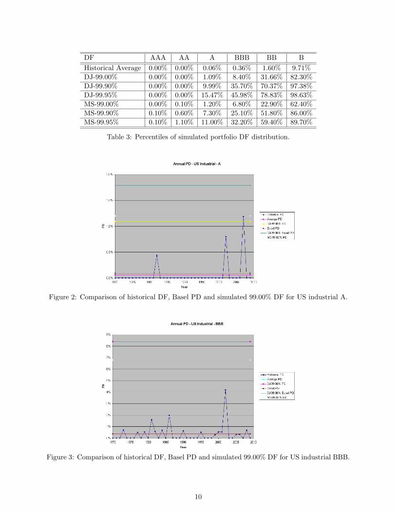
The pairwise asset correlation for US industrial sector applied in our simulation is 60%, which isestimated according to equity index. The 99.00%, 99.90% and 99.95% percentiles of the simulatedportfolio default frequency (DF) distribution are shown in Table 3 , where “DJ” and “MS” standfor direct jump simulation and multiple (monthly) step simulation, respectively.
In figures 2 to 5 we show the historical DF data, the average PD, Basel PD, above simulated99.00%-percentile DFs, and the 99.90%-percentile DFs with Basel PD by direct jump simulationfor ratings A, BBB, BB and B.
The difference of the 99.00%-percentiles of DF distributions using Moody’s TPM and Basel PDis significant except for rating BBB. The relative difference of the two percentiles reaches thelevel of 50% for rating A though the difference between Basel PD and Moody’s PD is only 3bps for this rating. Moreover, it appears that our simulated DF results for A rating are reasonablecompared with historical data as there is only one historical DF point within the period 1970−2009reaching the level of simulated 99.00%-percentile. Furthermore, our simulated DF results are very
9
DF AAA AA A BBB BB B
Historical Average 0.00% 0.00% 0.06% 0.36% 1.60% 9.71%
DJ-99.00% 0.00% 0.00% 1.09% 8.40% 31.66% 82.30%
DJ-99.90% 0.00% 0.00% 9.99% 35.70% 70.37% 97.38%
DJ-99.95% 0.00% 0.00% 15.47% 45.98% 78.83% 98.63%
MS-99.00% 0.00% 0.10% 1.20% 6.80% 22.90% 62.40%
MS-99.90% 0.10% 0.60% 7.30% 25.10% 51.80% 86.00%
MS-99.95% 0.10% 1.10% 11.00% 32.20% 59.40% 89.70%
Table 3: Percentiles of simulated portfolio DF distribution.
Figure 2: Comparison of historical DF, Basel PD and simulated 99.00% DF for US industrial A.
Figure 3: Comparison of historical DF, Basel PD and simulated 99.00% DF for US industrial BBB.
10

Figure 4: Comparison of historical DF, Basel PD and simulated 99.00% DF for US industrial BB.
Figure 5: Comparison of historical DF, Basel PD and simulated 99.00% DF for US industrial B.
11
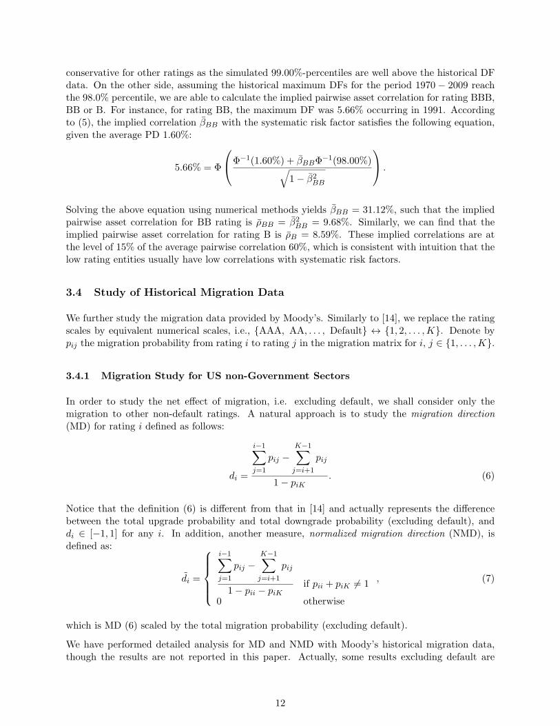
conservative for other ratings as the simulated 99.00%-percentiles are well above the historical DFdata. On the other side, assuming the historical maximum DFs for the period 1970 − 2009 reachthe 98.0% percentile, we are able to calculate the implied pairwise asset correlation for rating BBB,BB or B. For instance, for rating BB, the maximum DF was 5.66% occurring in 1991. Accordingto (5), the implied correlation �BB with the systematic risk factor satisfies the following equation,given the average PD 1.60%:
5.66% = Φ
⎛
⎝
Φ−1(1.60%) + �BBΦ−1(98.00%)
√
1− �2BB
⎞
⎠ .
Solving the above equation using numerical methods yields �BB = 31.12%, such that the impliedpairwise asset correlation for BB rating is �BB = �2
BB = 9.68%. Similarly, we can find that theimplied pairwise asset correlation for rating B is �B = 8.59%. These implied correlations are atthe level of 15% of the average pairwise correlation 60%, which is consistent with intuition that thelow rating entities usually have low correlations with systematic risk factors.
3.4 Study of Historical Migration Data
We further study the migration data provided by Moody’s. Similarly to [14], we replace the ratingscales by equivalent numerical scales, i.e., {AAA, AA, . . . , Default} ↔ {1, 2, . . . ,K}. Denote bypij the migration probability from rating i to rating j in the migration matrix for i, j ∈ {1, . . . ,K}.
3.4.1 Migration Study for US non-Government Sectors
In order to study the net effect of migration, i.e. excluding default, we shall consider only themigration to other non-default ratings. A natural approach is to study the migration direction(MD) for rating i defined as follows:
di =
i−1∑
j=1
pij −K−1∑
j=i+1
pij
1− piK. (6)
Notice that the definition (6) is different from that in [14] and actually represents the differencebetween the total upgrade probability and total downgrade probability (excluding default), anddi ∈ [−1, 1] for any i. In addition, another measure, normalized migration direction (NMD), isdefined as:
di =
⎧
⎨
⎩
i−1∑
j=1
pij −K−1∑
j=i+1
pij
1− pii − piKif pii + piK ∕= 1
0 otherwise
, (7)
which is MD (6) scaled by the total migration probability (excluding default).
We have performed detailed analysis for MD and NMD with Moody’s historical migration data,though the results are not reported in this paper. Actually, some results excluding default are
12

counterintuitive because the downgrade probability is underestimated in the case that a largeportion of downgrade falls directly into the category of default. Hence, we need to study themigration including default.
We shall now consider default case as a type of migration (downgrade). Then the total migrationdirection (TMD) for rating i is defined as
d(t)i =
i−1∑
j=1
pij −K∑
j=i+1
pij . (8)
In addition, di ∈ [−1, 1] for any i. The normalized total migration direction (NTMD) is defined as
d(t)i =
⎧
⎨
⎩
d(t)i
1− piiif pii ∕= 1
0 otherwise
, (9)
which is TMD (8) scaled by the total migration probability (including default).
Historical TMD/NTMD time series for the pool of all US sectors (excluding government) withinthe period 1970− 2009 are shown in figures 6 and 7 except for AAA in the normalized case (as it iseither 0 or −100%). The correlations of the TMD and NTMD time-series between different ratingsare reported in the two matrices in Tables 4 and 5 (excluding AAA for normalized case).
Figure 6: Correlation between US non-government TMD time series.
For the TMD time-series, strong correlation between all adjacent ratings can be observed (in boldfont), which is consistent with intuition. However, this is not obvious for NTMD correlation matrixfor high ratings, possibly due to the “amplification effect” of the normalization for tiny migrationprobability. Furthermore, we present the correlations between the historical DF time-series reportedby Moody’s and the TMD/NTMD time-series as shown in Table 6 (except for AAA because itsDF is always 0). In this way, the strong correlation between TMD and DF can be observed, andin general, we notice that this correlation is higher for lower ratings, which is also consistent withintuition.
13

Figure 7: Correlation between US non-government NTMD time series.
Correlation-TMD AAA AA A BBB BB B
AAA 100.00%
AA 55.81 100.00%
A 34.34% 67.20% 100.00%
BBB -3.27% 22.75% 54.97% 100.00%
BB 20.06% 52.28% 55.39% 48.46% 100.00%
B 8.08% 55.26% 58.55% 57.74% 57.46% 100.00%
Table 4: Correlation between US non-government TMD time series.
Correlation-NTMD AA A BBB BB B
AA 100.00%
A 2.47% 100.00%
BBB -4.67% 34.28% 100.00%
BB 32.65% 11.92% 25.58% 100.00%
B 38.04% 26.89% 37.62% 50.34% 100.00%
Table 5: Correlation between US non-government NTMD time series.
Rating AA A BBB BB B
Correlation-DF/TMD -39.29% -29.26% -63.88% -73.65% -85.16%
Correlation-DF/NTMD -11.52% -12.31% -49.84% -65.47% -73.42%
Table 6: Correlation between US non-government TMD/NTMD and DF time series.
14

Correlation-TMD AAA AA A BBB BB B
AAA 100.00%
AA 5.35% 100.00%
A 11.33% 56.52% 100.00%
BBB 7.68% 32.33% 66.43% 100.00%
BB 4.23% 29.74% 51.40% 65.77% 100.00%
B -5.60% -6.00% 23.40% 21.24% 27.23% 100.00%
Table 7: Correlation between US industrial sector TMD time series.
Rating A BBB BB B
Correlation-DF/TMD -44.54% -50.37% -66.98% -87.45%
Table 8: Correlation between US industrial sector TMD and DF time series.
3.4.2 Simulation of Total Migration Direction for US Industrial Sector
We further compare historical TMD data with multiple (monthly) step simulation results for USindustrial sector, which has the best coverage in Moody’s database. The simulation is performedin a similar way to that of the PD simulation as described in section 3.2 but we now simulate themigration events (including default events) at the end of the time horizon (one year). The pairwiseasset correlation is 60% as in section 3.3.
First, the historical TMD time-series of different ratings imply the correlation matrix given in Table7. Unlike the case of the whole US non-government pool, Table 7 does not show strong correlationbetween AAA and AA. This is probably due to the small number of AAA event counts (see Section3.3). The correlations between TMD and DF time-series are shown in Table 8 except for AAA andAA ratings because there was no default event, which is intuitive and consistent with the resultsof whole US non-government pool.
Our simulated percentiles of the portfolio TMD distribution are shown in Table 9. For A and BBBratings, the simulated TMDs are smaller, which is consistent with the weighted average migrationmatrix provided by Moody’s. The simulated 99.00% percentiles of the portfolio’s TMD distributionare shown in figures 8 to 13, to be compared with historical data.
It is worth noting that our average simulated TMDs are very close to the historical average. How-
TMD AAA AA A BBB BB B
Historical Average -8.31% -7.74% -4.31% -3.23% -4.96% -4.64%
MS Average -8.39% -7.79% -4.34% -3.18% -4.93% -4.62%
DJ-99.00% -78.36% -79.91% -70.12% -73.38% -81.89% -82.30%
DJ-99.90% -96.38% -96.79% -93.83% -94.91% -97.28% -97.38%
DJ-99.95% -98.04% -98.28% -96.45% -97.14% -98.57% -98.63%
MS-99.00% -59.00% -59.50% -49.80% -51.90% -60.70% -61.10%
MS-99.90% -84.60% -84.80% -78.50% -79.00% -85.40% -86.70%
MS-99.95% -89.50% -89.10% -84.80% -84.40% -90.00% -91.10%
Table 9: Percentiles of simulated portfolio TMD distribution.
15

Figure 8: Comparison of historical TMD and simulated 99.00% TMD for US industrial AAA.
Figure 9: Comparison of historical TMD and simulated 99.00% TMD for US industrial AA.
16

Figure 10: Comparison of historical TMD and simulated 99.00% TMD for US industrial A.
Figure 11: Comparison of historical TMD and simulated 99.00% TMD for US industrial BBB.
17

Figure 12: Comparison of historical TMD and simulated 99.00% TMD for US industrial BB.
Figure 13: Comparison of historical TMD and simulated 99.00% TMD for US industrial B.
18

Correlation-TMR AAA AA A BBB BB B
AAA 100.00%
AA -7.40% 100.00%
A 20.21% 42.90% 100.00%
BBB 7.19% 39.36% 82.40% 100.00%
BB 12.19% 20.88% 67.10% 67.30% 100.00%
B 24.68% 20.58% 37.04% 24.70% 31.35% 100.00%
Table 10: Correlation between US industrial sector TMR time series.
Rating A BBB BB B
Correlation-PD/TMR 35.84% 29.11% 55.13% 80.67%
Table 11: Correlation between US industrial sector TMR and DF time series.
ever, our simulated 99.00% percentiles of portfolio TMD distribution, in particular those of thedirect jump simulation, are conservative compared with historical data. We have further performedmultiple step simulation with a grid of pairwise asset correlations ranging from 0% to 60% for eachrating to compare with historical data. It appears that for ratings other than AAA, the pairwiseasset correlation implied by the simulation results (compared with historical data) is around 30%2.
3.4.3 Simulation of Total Migration Rate for US Industrial Sector
In practice, we may have various positions in a credit portfolio, so it is possible that the upgrade ofunderlying entity may lead to loss. Therefore, we are interested in not only the migration directionbut also the total migration amount, regardless of upgrade or downgrade events, which is definedas total migration rate (TMR) as follows:
ri = 1− pii. (10)
Clearly, TMR is non-negative. Furthermore, at tail scenarios (e.g., 99.90% percentile of portfolioTMR distribution), TMR should be slightly larger than the absolute value of TMD, because thereexists tiny upgrade probability in that case. We follow a similar approach to the previous studyfor TMR. The correlation matrix of historical TMR time-series of different ratings of US Industrialsector is given in Table 10.
We can again observe the strong correlation between adjacent ratings except for the pair of AAAand AA. The correlations between the TMR and DF time-series are shown in Table 11 except forAAA and AA ratings (because there was no default event for them), which is again consistent withthe results of TMD of US Industrial sector.
Our simulated 99.90% percentiles of portfolio TMR distribution are given in Table 12. The resultsconfirm our expectation that TMRs are slightly larger than the absolute value of TMDs. Thesimulation averages are also very close to the historical averages. The above simulated 99.90%percentiles of portfolio TMR distribution are compared with historical data as shown in figures 14to 19.
2The detailed results are not reported here due to limited space; however, the approach is straightforward.
19

TMR AAA AA A BBB BB B
Historical Average 8.31% 9.90% 8.08% 10.64% 14.11% 14.77%
MS Average 8.39% 9.98% 8.12% 10.63% 14.11% 14.78%
DJ-99.00% 78.90% 80.50% 72.00% 77.60% 84.90% 85.50%
DJ-99.90% 96.80% 97.40% 94.30% 95.60% 97.70% 97.90%
DJ-99.95% 98.20% 98.70% 96.60% 97.40% 99.00% 99.00%
MS-99.00% 59.00% 60.50% 52.60% 58.20% 65.70% 68.90%
MS-99.90% 84.60% 85.30% 79.60% 82.10% 86.80% 89.50%
MS-99.95% 89.50% 89.30% 85.60% 86.70% 91.10% 93.40%
Table 12: Percentiles of simulated portfolio TMR distribution.
Figure 14: Comparison of historical TMR and simulated 99.00% TMR for US industrial AAA.
Figure 15: Comparison of historical TMR and simulated 99.00% TMR for US industrial AA.
20

Figure 16: Comparison of historical TMR and simulated 99.00% TMR for US industrial A.
Figure 17: Comparison of historical TMR and simulated 99.00% TMR for US industrial BBB.
21

Figure 18: Comparison of historical TMR and simulated 99.00% TMR for US industrial BB.
Figure 19: Comparison of historical TMR and simulated 99.00% TMR for US industrial B.
22

In general, our simulation results are conservative. For the AAA rating, there were only 16 eventcounts in the year 1982, which does not provide a sufficient sample for our study.
4 Annual TPM Construction
This section discusses how we combine the TPM generated by Moody’s shown in Table 1 and BaselPDs, through all steps of the calculation.
4.1 Setting the PDs
Once we obtained Moody’s TPM we tested the effect of replacing Moody’s original PDs with otherPDs: Basel PD and Basel maximum PD. Normally banks have a mapping between rating agencies’ratings and internal ratings that Basel PDs are assigned. Labeling the internal rating from 1 to 25,such a mapping is shown in Table 13. As shown in the table, the IRC ratings can be defined.
IRC Alphabetic S&P Moody’s Internal Ratings
AAA AAA AAA 1
AA AA+ AA1 2
AA AA AA2 3
AA AA- AA3 4
A A+ A1 5
A A A2 6
A A- A3 7
BBB BBB+ BAA1 8
BBB BBB BAA2 9
BBB BBB- BAA3 10
BB BB+ BA1 11
BB BB BA2 12
BB BB- BA3 13
B B+ B1 14
B B B2 15
B B- B3 16
CCC CCC+ CAA1 17
CCC CCC CAA2 18
CCC CCC- CAA3 19
D CC CA 20
D C C 21
D UNRATE UNRATE 22
D NR UNRATE 23
D (None) (None) 24
D D D 25
Table 13: Relationship between different rating schemes: IRC Alphabetic, S&P, Moody’s, internal.
23
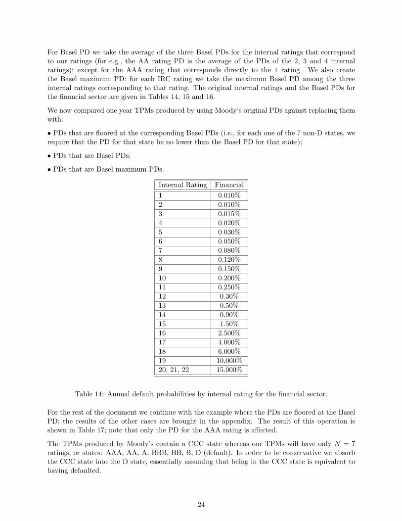
For Basel PD we take the average of the three Basel PDs for the internal ratings that correspondto our ratings (for e.g., the AA rating PD is the average of the PDs of the 2, 3 and 4 internalratings); except for the AAA rating that corresponds directly to the 1 rating. We also createthe Basel maximum PD: for each IRC rating we take the maximum Basel PD among the threeinternal ratings corresponding to that rating. The original internal ratings and the Basel PDs forthe financial sector are given in Tables 14, 15 and 16.
We now compared one year TPMs produced by using Moody’s original PDs against replacing themwith:
∙ PDs that are floored at the corresponding Basel PDs (i.e., for each one of the 7 non-D states, werequire that the PD for that state be no lower than the Basel PD for that state);
∙ PDs that are Basel PDs;
∙ PDs that are Basel maximum PDs.
Internal Rating Financial
1 0.010%
2 0.010%
3 0.015%
4 0.020%
5 0.030%
6 0.050%
7 0.080%
8 0.120%
9 0.150%
10 0.200%
11 0.250%
12 0.30%
13 0.50%
14 0.90%
15 1.50%
16 2.500%
17 4.000%
18 6.000%
19 10.000%
20, 21, 22 15.000%
Table 14: Annual default probabilities by internal rating for the financial sector.
For the rest of the document we continue with the example where the PDs are floored at the BaselPD; the results of the other cases are brought in the appendix. The result of this operation isshown in Table 17; note that only the PD for the AAA rating is affected.
The TPMs produced by Moody’s contain a CCC state whereas our TPMs will have only N = 7ratings, or states: AAA, AA, A, BBB, BB, B, D (default). In order to be conservative we absorbthe CCC state into the D state, essentially assuming that being in the CCC state is equivalent tohaving defaulted.
24

Internal Rating Financial
AAA 0.010%
AA 0.015%
A 0.05%
BBB 0.16%
BB 0.387%
B 1.713%
CCC 6.667%
Table 15: Basel annual default probabilities by rating for the financial sector.
Internal Rating Financial
AAA 0.010%
AA 0.020%
A 0.080%
BBB 0.200%
BB 0.50%
B 2.500%
CCC 10.000%
Table 16: Basel maximum annual default probabilities by rating for the financial sector.
We do this operation by first deleting the CCC row; we then add the probabilities of the CCCcolumn to the D column, and finally delete the CCC column.
The result of removing the CCC state is shown in Table 18.
Note that for consistency sake we first replaced the Basel PDs and only then removed the CCCstate: the source of the Basel PDs is in a context of a TPM where 7 states exist; it would besomewhat improper to do these operations in reverse order since then we would be bringing in PDsfrom a 7-state TPM to replace PDs in a 6-state TPM. Table 13 shows the mapping between theAlphanumeric states to the 7-Alphabetic states.
4.2 TPM Rescaling
Had we only performed the operation in the previous step then all rows in the new 7-state TPMwould still sum up to unity; but since we replaced some of the PDs this is no longer the case.To ensure that every row sums to 1, we now remove the excess between the sum of each row andunity from its diagonal entry. Denoting the TPM elements in Table 18 by aij the rescaled elementsbecome:
aii = aii +
⎛
⎝1−N∑
j=1,j ∕=i
aij
⎞
⎠ . (11)
The result of this operation is shown in Table 19; the only elements affected were a11, a55 and a66.
25

AAA AA A BBB BB B CCC D
AAA 88.24% 11.76% 0.00% 0.00% 0.00% 0.00% 0.00% 0.01%
AA 0.64% 91.11% 8.13% 0.08% 0.01% 0.00% 0.00% 0.03%
A 0.03% 5.59% 88.36% 4.99% 0.79% 0.15% 0.02% 0.07%
BBB 0.00% 1.16% 15.85% 76.40% 5.28% 0.70% 0.00% 0.61%
BB 0.00% 0.00% 2.13% 11.93% 77.46% 6.23% 0.99% 1.27%
B 0.00% 0.00% 0.62% 1.99% 16.69% 70.17% 7.30% 3.22%
CCC 0.00% 0.00% 0.00% 0.00% 4.17% 20.83% 29.56% 45.44%
D 0 0 0 0 0 0 0 100%
Table 17: Annual TPM obtained from Table 1 by replacing the original PDs with the Basel PDswhenever the latter were bigger.
AAA AA A BBB BB B D
AAA 88.24% 11.76% 0.00% 0.00% 0.00% 0.00% 0.01%
AA 0.64% 91.11% 8.13% 0.08% 0.01% 0.00% 0.03%
A 0.03% 5.59% 88.36% 4.99% 0.79% 0.15% 0.09%
BBB 0.00% 1.16% 15.85% 76.40% 5.28% 0.70% 0.61%
BB 0.00% 0.00% 2.13% 11.93% 77.46% 6.23% 2.26%
B 0.00% 0.00% 0.62% 1.99% 16.69% 70.17% 10.52%
D 0 0 0 0 0 0 100%
Table 18: Annual TPM from Table 17 after removing the CCC state.
The rescaling done in (11) is only one possible way of rescaling the TPM, and was also followed in[11]. Another possible rescaling is to rescale all elements in every row, except the PD, such thatthe element aij of the pre-scaled annual TPM becomes
aij = aij +
⎛
⎝1− PDi −N−1∑
j=1
aij
⎞
⎠
aij∑N−1
j=1 aij,
where PDi is the PD of state i. This ensures that for every row i we have∑N
j=1 aij =∑N−1
j=1 aij +PDi = 1. The drawback of this rescaling as compared to (11) is that it might decrease downgradingprobabilities in the row; this would mean that (although retaining the relative strength of all non-PDprobabilities in the row) less absolute probability is given to downgrade events than in the originalTPM. This would thus translate into less capital being necessary, hence being less conservative.When only diagonal elements are modified in each row this issue does not arise.
Alternatively, in [8] (JLT) and [10] a different approach is considered for replacing the originalPDs. Consider a generator matrix Λ produced from the TPM in the previous stages - this is‘simply’ the logarithm of the TPM; see section 5.1 and also [11] for more discussion. In orderto modify the PDs of the original TPM a transformation is performed on Λ: Λ = UΛ whereU = diag(�(1), �(2), . . . , �(N)) with �(N) ≡ 1. The new annual TPM, with the modified PDs, is
now given by ˜TPM = eΛ. A numerical algorithm is employed to solve for U such that the lastcolumn of ˜TPM matches the new required PDs. Several other equally good methods have been
26

AAA AA A BBB BB B D
AAA 88.23% 11.76% 0.00% 0.00% 0.00% 0.00% 0.01%
AA 0.64% 91.11% 8.13% 0.08% 0.01% 0.00% 0.03%
A 0.03% 5.59% 88.36% 4.99% 0.79% 0.15% 0.09%
BBB 0.00% 1.16% 15.85% 76.40% 5.28% 0.70% 0.61%
BB 0.00% 0.00% 2.13% 11.93% 77.45% 6.23% 2.26%
B 0.00% 0.00% 0.62% 1.99% 16.69% 70.18% 10.52%
D 0 0 0 0 0 0 100%
Table 19: Annual TPM after rescaling the TPM in Table 18 according to (11).
proposed to mimic the same effect of replacing the PDs and all suffer from modelling uncertainty.In Table 20 we show the parameters used for the JLT model and Tables 21 – 26 compare the resultsfor the annual and one month TPMs to the JLT results.
�(i) Calibrated PD Input PD Discrepancy Original PD
AAA 1.117641 0.010% 0.010% 0.00E+00 0.00%
AA 0.483725 0.015% 0.015% 0.00E+00 0.03%
A 1.01256 0.073% 0.073% 0.00E+00 0.09%
BBB 0.245935 0.157% 0.157% 0.00E+00 0.61%
BB 0.607434 1.377% 1.377% 0.00E+00 2.26%
B 0.841143 9.013% 9.013% 0.00E+00 10.52%
Table 20: JLT model calibration parameters, Basel PDs and Moody’s TPM implied PD.
AAA AA A BBB BB B D
AAA 88.24% 11.76% 0.00% 0.00% 0.00% 0.00% 0.01%
AA 0.64% 91.11% 8.13% 0.08% 0.01% 0.00% 0.03%
A 0.03% 5.59% 88.36% 4.99% 0.79% 0.15% 0.09%
BBB 0.00% 1.16% 15.85% 76.40% 5.28% 0.70% 0.61%
BB 0.00% 0.00% 2.13% 11.93% 77.46% 6.23% 2.26%
B 0.00% 0.00% 0.62% 1.99% 16.69% 70.17% 10.52%
D 0 0 0 0 0 0 100 %
Table 21: Annual TPM for the financial sector consistent with Basel PDs: original TPM – comparewith Table A5 in the appendix.
5 Monthly or Quarterly TPM Construction
5.1 TPM Construction via Generator Matrix
We now take the natural logarithm of the annual TPM resulting from the previous step to create thegenerator: G = log(TPM). In general, this operation will create negative values in the off-diagonal
27

AAA AA A BBB BB B D
AAA 86.6293% 13.0519% 0.2811% 0.0242% 0.0029% 0.0007% 0.0100%
AA 0.3110% 95.5472% 3.9851% 0.1233% 0.0155% 0.0028% 0.0150%
A 0.0200% 5.7718% 87.7239% 5.5732% 0.7074% 0.1304% 0.0733%
BBB 0.0007% 0.3203% 4.3034% 93.5348% 1.5116% 0.1725% 0.1567%
BB 0.0003% 0.0317% 0.7887% 8.4326% 85.3023% 4.0677% 1.3767%
B 0.0001% 0.0133% 0.3953% 1.4078% 15.1750% 73.9951% 9.0133%
D 0 0 0 0 0 0 100 %
Table 22: Annual TPM for the financial sector consistent with Basel PDs: JLT TPM.
AAA AA A BBB BB B D
AAA -1.6107% 1.2919% 0.2811% 0.0242% 0.0029% 0.0007% 0.0000%
AA -0.3290% 4.4372% -4.1449% 0.0433% 0.0055% 0.0028% -0.0150%
A -0.0100% 0.1818% -0.6361% 0.5832% -0.0826% -0.0196% -0.0167%
BBB 0.0007% -0.8397% -11.5466% 17.1348% -3.7684% -0.5275% -0.4533%
BB 0.0003% 0.0317% -1.3413% -3.4974% 7.8423% -2.1623% -0.8833%
B 0.0001% 0.0133% -0.2247% -0.5822% -1.5150% 3.8251% -1.5067%
D 0 0 0 0 0 0 0
Table 23: Annual TPM for the financial sector consistent with Basel PDs: Table 21 minus Table22.
elements of G, gij i ∕= j, so we first floor all negative off-diagonal elements with 0:
gij −→{
0 if i ∕= j and gij < 0
gij else.(12)
Then we adjust the non-zero elements according to their relative magnitude in the row: denote thematrix G whose elements are given by:
gij = ∣gij ∣∑N
j=1 gij∑N
j=1 ∣gij ∣(13)
and setG = G− G. (14)
All rows of G now properly sum to zero. The result of taking the logarithm of the TPM in Table19 is shown in Table 27; after performing the operations in (12) – (14) we obtain the generator inTable 28.
The final 1-month TPM resulting from all this is given by exponentiating 112G:
TPM1−month = exp
(
1
12G
)
. (15)
Similarly, by exponentiating G/4 we can obtain a quarterly TPM. Table 29 shows the final TPM1−month
for the financial sector.
28

AAA AA A BBB BB B D
AAA 0.989339 0.010596 3.99E-05 1.49E-05 1.75E-06 4.4E-07 7.26E-06
AA 0.000583 0.991937 0.007434 1.87E-05 2.33E-06 4.23E-07 2.39E-05
A 1.12E-05 0.00514 0.989099 0.004958 0.000625 0.000113 5.26E-05
BBB 2.76E-07 0.000685 0.015814 0.976955 0.005513 0.00055 0.000482
BB 3.89E-07 6.7E-06 0.001012 0.012625 0.977788 0.006851 0.001717
B 5.77E-09 1.29E-06 0.000395 0.000864 0.018471 0.970173 0.010096
D 0 0 0 0 0 0 1
Table 24: Monthly TPM for the financial sector consistent with Basel PDs: original TPM – comparewith Table A8 in the appendix.
AAA AA A BBB BB B D
AAA 0.988091 0.01186 2.15E-05 1.68E-05 1.92E-06 4.85E-07 8.03E-06
AA 0.000282 0.996092 0.003603 9.21E-06 1.14E-06 2.05E-07 1.16E-05
A 1.05E-05 0.005214 0.988923 0.005063 0.000625 0.000113 5.20E-05
BBB 4.32E-08 0.000171 0.003923 0.994279 0.001374 0.000135 0.000119
BB 2.36E-07 2.12E-06 0.000571 0.007771 0.986425 0.004188 0.001043
B 3.54E-09 9.09E-07 0.000326 0.000695 0.015642 0.974829 0.008507
D 0 0 0 0 0 0 1
Table 25: Monthly TPM for the financial sector consistent with Basel PDs: JLT TPM.
5.2 TPM Construction via QOM
In [11] a quasi-optimization method (QOM) is proposed to find the best approximation of one-monthTPM, in the sense that it is ‘closest’ and has all the properties of a TPM, to a given root of someTPM; in general, such a root does not have the properties of a TPM. Denoting this approximateTPM by X, with rows xi = (xi1, xi2, . . . , xiN , ), and the root of the original TPM by Y = TPM1/12,
with rows yi = (yi1, yi2, . . . , yiN , ), we need to minimize dist(yi, xi) =√
∑Nj=1(yij − xij)2 and also
meet∑N
j=1 xij = 1. In Tables 30 – 32 we show the results of implementing this approach. A detailedseven-step procedure can be found in [11]. Note the small difference between the two approaches,essentially giving results of the same order of magnitude, while bearing in mind the more complexnature of the QOM scheme.
5.3 Error Control
In order to test the quality of the output monthly TPM we compare TPM121−month to the annual
TPM from Table 19 which was used to construct the generator; Table 33 shows the differencebetween these two matrices in percent. Table 34 shows the relative difference between these twomatrices.
We use the following matrix norms as a measure of the distance between the monthly TPM of
29

AAA AA A BBB BB B D
AAA 0.001248 -0.00126 1.83E-05 -1.90E-06 -1.70E-07 -4.60E-08 -7.70E-07
AA 0.000301 -0.00415 0.003831 9.46E-06 1.20E-06 2.17E-07 1.23E-05
A 6.56E-07 -7.40E-05 0.000177 -0.0001 2.42E-07 2.15E-07 5.97E-07
BBB 2.33E-07 0.000515 0.011891 -0.01732 0.00414 0.000415 0.000363
BB 1.52E-07 4.58E-06 0.000442 0.004854 -0.00864 0.002662 0.000674
B 2.23E-09 3.77E-07 6.90E-05 0.000169 0.002829 -0.00466 0.001589
D 0 0 0 0 0 0 0
Table 26: Monthly TPM for the financial sector consistent with Basel PDs: Table 24 minus Table25.
AAA AA A BBB BB B D
AAA -12.5696% 13.1447% -0.6051% 0.0186% 0.0021% 0.0005% 0.0088%
AA 0.7138% -9.6363% 9.1061% -0.1838% -0.0223% -0.0063% 0.0289%
A 0.0117% 6.2251% -13.2248% 6.0481% 0.7447% 0.1345% 0.0607%
BBB -0.0056% 0.7855% 19.3005% -28.0677% 6.7580% 0.6536% 0.5757%
BB 0.0005% -0.1247% 1.1121% 15.5310% -27.0168% 8.4560% 2.0420%
B -8.05⋅10−6% -0.0153% 0.4648% 0.9171% 22.7612% -36.4100% 12.2822%
D 0 0 0 0 0 0 0
Table 27: The generator G after taking the natural logarithm of the TPM in Table 19; results havebeen rounded to nearest displayed accuracy. Note that the elements g13, g24, g25, g26, g41, g52, g61,g62 will be nullified in the next step.
Table 29 raised to the 12-th power and the annual TPM of Table 19:
∥A∥1 = max1≤j≤N
N∑
i=1
∣aij ∣, (the maximum of absolute column sum), (16)
∥A∥2 =√
�max(ATA), (17)
∥A∥∞ = max1≤i≤N
N∑
j=1
∣aij ∣, (the maximum of absolute row sum), (18)
∥A∥Frobenius =
√
√
√
⎷
N∑
i,j=1
∣aij ∣2 =√
trace(ATA), (19)
where �max(ATA) is the largest eigenvalue of ATA. These results are shown in Table 35. Note
that though the difference seems large at first, it is actually an exaggeration of the difference:∥A∥Frobenius, for e.g., should really be divided by 72 = 49, the number of elements in the matrix,to get an estimate of the typical size of the elements in Table 33.
30

AAA AA A BBB BB B D
AAA -12.8651% 12.8358% 0 0.0181% 0.0021% 0.0005% 0.0086%
AA 0.7060% -9.7414% 9.0068% 0 0 0 0.0286%
A 0.0117% 6.2251% -13.2248% 6.0481% 0.7447% 0.1345% 0.0607%
BBB 0 0.7854% 19.2986% -28.0704% 6.7573% 0.6535% 0.5756%
BB 0.0005% 0 1.1095% 15.4952% -27.0790% 8.4365% 2.0373%
B 0 0 0.4647% 0.9169% 22.7564% -36.4177% 12.2796%
D 0 0 0 0 0 0 0
Table 28: The generator G after rescaling the generator in Table 27 according to (12) – (14); resultshave been rounded to nearest displayed accuracy.
AAA AA A BBB BB B D
AAA 98.9339% 1.0596% 0.0040% 0.0015% 0.0002% 4.39⋅10−5% 0.0007%
AA 0.0583% 99.1937% 0.7434% 0.0019% 0.0002% 4.23⋅10−5% 0.0024%
A 0.0011% 0.5140% 98.9099% 0.4958% 0.0625% 0.0113% 0.0053%
BBB 2.76⋅10−5% 0.0685% 1.5814% 97.6955% 0.5513% 0.0550% 0.0482%
BB 3.89⋅10−5% 0.0007% 0.1012% 1.2625% 97.7788% 0.6851% 0.1717%
B 5.77⋅10−7% 0.0001% 0.0395% 0.0864% 1.8471% 97.0173% 1.0096%
D 0 0 0 0 0 0 100%
Table 29: Monthly TPM for the financial sector after exponentiating the generator G in Table 28according to (15).
AAA AA A BBB BB B D
AAA 0.989366 0.010634 0 0 0 0 0
AA 0.000546 0.991982 0.007472 0 0 0 0
A 1.12E-05 0.00514 0.9891 0.004958 0.000625 0.000113 5.26E-05
BBB 0 0.000684 0.015814 0.976957 0.005513 0.00055 0.000481
BB 0 0 0.000995 0.012635 0.97782 0.006848 0.001702
B 0 0 0.000392 0.000862 0.018473 0.970177 0.010095
D 0 0 0 0 0 0 1
Table 30: Monthly TPM for the financial sector: using the QOM scheme.
AAA AA A BBB BB B D
AAA -2.60E-05 -3.80E-05 3.99E-05 1.49E-05 1.75E-06 4.40E-07 7.26E-06
AA 3.65E-05 -4.40E-05 -3.80E-05 1.87E-05 2.33E-06 4.23E-07 2.39E-05
A -6.50E-09 -1.90E-07 -2.10E-07 3.77E-07 3.06E-08 8.07E-09 -2.00E-09
BBB 2.76E-07 9.30E-07 -9.10E-07 -1.60E-06 2.22E-08 6.12E-07 6.52E-07
BB 3.89E-07 6.70E-06 1.71E-05 -1.00E-05 -3.20E-05 3.06E-06 1.51E-05
B 5.77E-09 1.29E-06 2.38E-06 1.97E-06 -2.00E-06 -3.90E-06 2.47E-07
D 0 0 0 0 0 0 0
Table 31: Monthly TPM for the financial sector: Table 24 minus Table 30.
31

QOM Generator approach
AAA 0.9689% 1.0894%
AA 0.3218% 0.3662%
A 0.0087% 0.0104%
BBB 0.0126% 0.0153%
BB 0.1953% 0.2110%
B 0.0428% 0.0476%
Table 32: Absolute row sum of the monthly TPM for the financial sector from Tables 24 and 30.
AAA AA A BBB BB B D
AAA -0.2616% -0.2831% 0.5152% 0.0250% 0.0037% 0.0008% 5.09⋅10−6%
AA -0.0082% -0.0988% -0.0760% 0.1520% 0.0240% 0.0063% 0.0008%
A -0.0001% -0.0025% -0.0025% 0.0046% 0.0005% 0.0001% -1.48⋅10−5%
BBB 0.0045% 0.0031% -0.0023% -0.0023% -0.0022% -0.0006% -0.0002%
BB 0.0007% 0.1048% -0.0008% -0.0314% -0.0507% -0.0166% -0.0059%
B 0.0001% 0.0234% 0.0003% -0.0038% -0.0096% -0.0072% -0.0031%
D 0 0 0 0 0 0 0
Table 33: The difference(
TPM121−month − TPM of Table 19
)
in percentage.
AAA AA A BBB BB B D
AAA -0.0030 -0.0241 – – – – 0.0005
AA -0.0129 -0.0011 -0.0093 1.9000 2.3982 – 0.0251
A -0.0038 -0.0005 -2.84⋅10−5 0.0009 0.0006 0.0007 -0.0002
BBB – 0.0027 -0.0001 -3.06⋅10−5 -0.0004 -0.0009 -0.0004
BB – – -0.0004 -0.0026 -0.0007 -0.0027 -0.0026
B – – 0.0005 -0.0019 -0.0006 -0.0001 -0.0003
D 0 0 0 0 0 0 0
Table 34: The relative error(
TPM121−month − TPM of Table 19
)
/ (TPM of Table 19); dash entriesrepresent cases where the TPM of Table 19 had a zero entry.
Norm Govt. Corp. Fin.
∥ ⋅ ∥1 0.5632% 0.0339% 0.5971%
∥ ⋅ ∥2 0.4742% 0.0419% 0.6460%
∥ ⋅ ∥∞ 0.8375% 0.0709% 1.0894%
∥ ⋅ ∥Frobenius 0.5752% 0.0485% 0.6853%
Table 35: Norms of the difference(
TPM121−month − TPM of Table 19
)
.
32

6 Discussion
This paper summarizes most of our exercise to compute TPMs for IRC. There are large uncertain-ties in the computed TPMs due to the lack of sufficiently accurate input data and the multipleways in which the matrices can be manipulated. Due to varying portfolio composition amongdifferent institutions we refrain from making specific recommendations on which method performsbest. Therefore, given the importance of TPMs and their PDs in the IRC, financial institutionswill need to make discretionary choices regarding their preferred methodology while ensuring thatuncertainties are well understood, managed and communicated properly to local regulators.
We also performed other tests and there are still several issues that we need to investigate further.For example, one of the spurious effects of the manipulations done on the annual generator is tointroduce non-zero probabilities in places that had zero probabilities in the original TPM; compare,for e.g., the elements in the first row of Table 29 to those in Table 19. These non-zero probabilitiesin the first row of Table 29 will introduce non-zero probabilities in the annual TPM in TPM12
1−month.This poses two problems that at the moment are not addressed. The obvious question is how tocorrect these non-zero probabilities that defy the zero probabilities in the original TPM. A moresubtle issue is the fact that since the original TPM is constructed from historic data it extractsprobabilities from a finite number of events; therefore, if we are to address the previous question,perhaps we should first bear in mind that from a formal perspective, a zero probability entryin the original TPM has, in fact, zero probability... The right thing to do is perhaps to replaceall zero entries in the original TPM with some error of the data, something like standard error∼ �/
√Nmeasurements. That way, the original input data will be given some error bars correcting
the misleading perception of its accuracy, and allowing for some leeway in manipulating it in aself-consistent manner.
There are several other future developments that we will continue to investigate. For example, wemay continue to look for any other available information that we can integrate to the estimationof TPM; better rating mapping methodologies; other statistic measures to understand the ratingmigration behavior, etc.
Finally, it may be worthwhile mentioning that the exercise reported in this report can be appliedto other projects such as counterparty economic capital calculation. Currently, most such com-putations are based on default only approach and a similar TPM is needed if we want to includemigration risk. Contrary to what we have done here, we may adjust sector and rating based TPMsto include idiosyncratic credit risk on the obligor level.
33

Appendix: TPMs
This appendix brings the relevant TPMs mentioned in the calculations in this document.
Moody’s TPMs
Tables A1 – A3 list the monthly TPMs generated from MCRC. These can be compared againstthe monthly TPMs resulting from our calculations.
AAA AA A BBB BB B CCC D
AAA 99.69% 0.30% 0.01% 0.00% 0.00% 0.00% 0.00% 0.00%
AA 0.30% 99.56% 0.13% 0.00% 0.00% 0.00% 0.00% 0.00%
A 0.04% 0.43% 99.34% 0.14% 0.05% 0.00% 0.00% 0.00%
BBB 0.00% 0.00% 0.45% 99.13% 0.40% 0.03% 0.00% 0.00%
BB 0.00% 0.00% 0.00% 0.64% 98.95% 0.36% 0.06% 0.00%
B 0.00% 0.00% 0.00% 0.00% 0.73% 97.95% 1.06% 0.26%
CCC 0.00% 0.00% 0.00% 0.00% 0.00% 0.64% 98.95% 0.41%
Table A1: Moody’s monthly TPM for the government sector.
AAA AA A BBB BB B CCC D
AAA 98.77% 1.23% 0.00% 0.00% 0.00% 0.00% 0.00% 0.00%
AA 0.10% 99.19% 0.70% 0.01% 0.00% 0.00% 0.00% 0.00%
A 0.01% 0.48% 99.03% 0.46% 0.02% 0.00% 0.00% 0.00%
BBB 0.00% 0.07% 1.41% 97.83% 0.62% 0.03% 0.01% 0.02%
BB 0.00% 0.04% 0.15% 1.16% 97.84% 0.76% 0.01% 0.04%
B 0.00% 0.00% 0.03% 0.13% 1.55% 97.13% 0.87% 0.28%
CCC 0.00% 0.00% 0.00% 0.00% 0.00% 2.14% 93.26% 4.61%
Table A2: Moody’s monthly TPM for the financial sector.
AAA AA A BBB BB B CCC D
AAA 99.06% 0.84% 0.09% 0.00% 0.00% 0.00% 0.00% 0.00%
AA 0.03% 99.03% 0.92% 0.02% 0.00% 0.00% 0.00% 0.00%
A 0.00% 0.09% 99.33% 0.56% 0.01% 0.00% 0.01% 0.00%
BBB 0.00% 0.00% 0.31% 99.25% 0.40% 0.03% 0.01% 0.00%
BB 0.00% 0.00% 0.03% 0.53% 98.34% 1.03% 0.03% 0.03%
B 0.00% 0.01% 0.01% 0.04% 0.45% 98.37% 0.77% 0.35%
CCC 0.00% 0.00% 0.00% 0.04% 0.06% 0.67% 96.30% 2.93%
Table A3: Moody’s monthly TPM for the corporate sector.
34

Tables A4 – A6 list the annual TPMs generated from MCRC. These are used as input for ourcalculations.
AAA AA A BBB BB B CCC D
AAA 96.50% 3.32% 0.00% 0.05% 0.12% 0.00% 0.00% 0.00%
AA 3.52% 94.97% 1.51% 0.00% 0.00% 0.00% 0.00% 0.00%
A 0.43% 5.22% 93.00% 1.13% 0.21% 0.00% 0.00% 0.00%
BBB 0.00% 0.00% 5.23% 89.98% 4.44% 0.36% 0.00% 0.00%
BB 0.00% 0.00% 0.00% 8.22% 86.64% 2.36% 2.56% 0.23%
B 0.00% 0.00% 0.00% 0.00% 8.33% 82.54% 6.62% 2.50%
CCC 0.00% 0.00% 0.00% 0.00% 0.00% 7.40% 89.57% 3.03%
Table A4: Moody’s annual TPM for the government sector.
AAA AA A BBB BB B CCC D
AAA 88.24% 11.76% 0.00% 0.00% 0.00% 0.00% 0.00% 0.00%
AA 0.64% 91.11% 8.13% 0.08% 0.01% 0.00% 0.00% 0.03%
A 0.03% 5.59% 88.36% 4.99% 0.79% 0.15% 0.02% 0.07%
BBB 0.00% 1.16% 15.85% 76.40% 5.28% 0.70% 0.00% 0.61%
BB 0.00% 0.00% 2.13% 11.93% 77.46% 6.23% 0.99% 1.27%
B 0.00% 0.00% 0.62% 1.99% 16.69% 70.17% 7.30% 3.22%
CCC 0.00% 0.00% 0.00% 0.00% 4.17% 20.83% 29.56% 45.44%
Table A5: Moody’s annual TPM for the financial sector.
AAA AA A BBB BB B CCC D
AAA 89.23% 9.82% 0.95% 0.00% 0.00% 0.00% 0.00% 0.00%
AA 0.35% 88.97% 10.20% 0.48% 0.00% 0.00% 0.00% 0.00%
A 0.03% 1.04% 92.16% 6.28% 0.35% 0.04% 0.05% 0.04%
BBB 0.01% 0.03% 3.76% 91.37% 3.90% 0.55% 0.25% 0.12%
BB 0.00% 0.02% 0.44% 6.17% 81.87% 9.33% 0.99% 1.18%
B 0.02% 0.04% 0.14% 0.51% 5.14% 81.92% 6.83% 5.39%
CCC 0.00% 0.00% 0.03% 0.00% 1.14% 8.22% 68.57% 22.03%
Table A6: Moody’s annual TPM for the corporate sector.
35
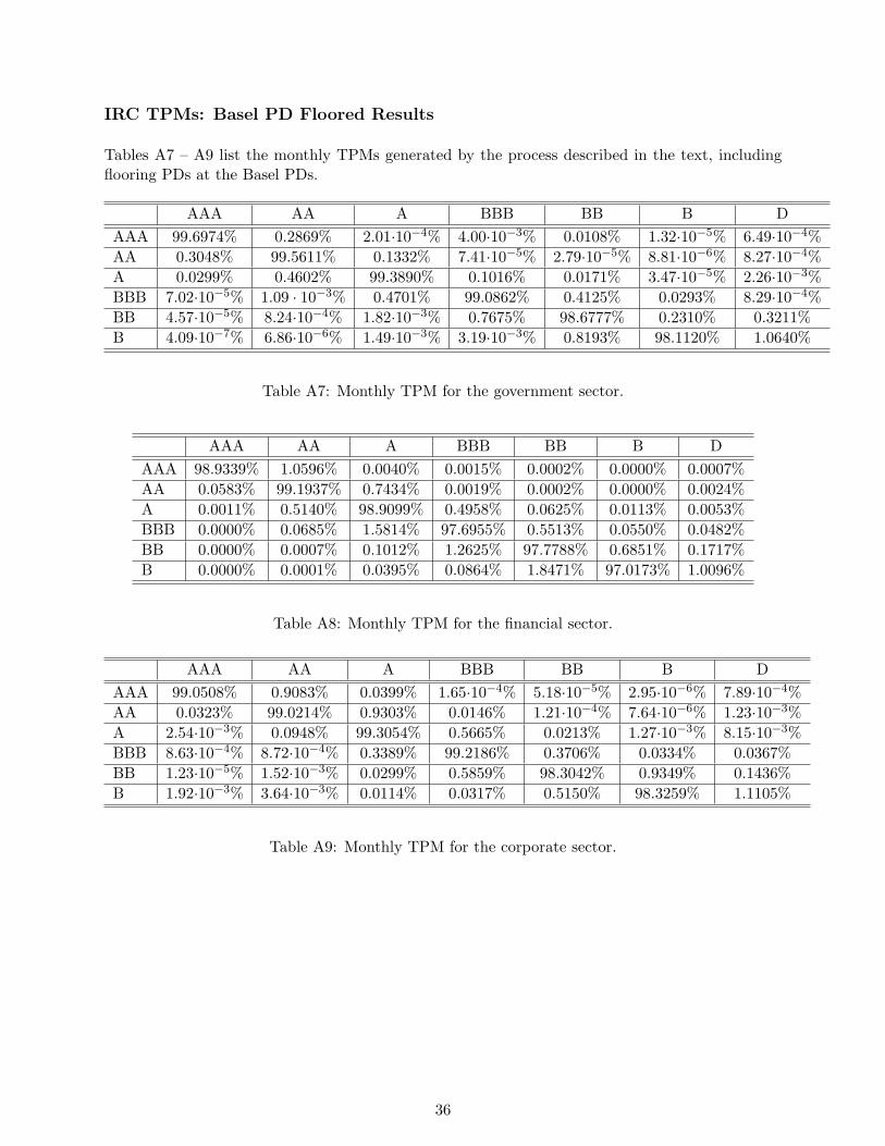
IRC TPMs: Basel PD Floored Results
Tables A7 – A9 list the monthly TPMs generated by the process described in the text, includingflooring PDs at the Basel PDs.
AAA AA A BBB BB B D
AAA 99.6974% 0.2869% 2.01⋅10−4% 4.00⋅10−3% 0.0108% 1.32⋅10−5% 6.49⋅10−4%
AA 0.3048% 99.5611% 0.1332% 7.41⋅10−5% 2.79⋅10−5% 8.81⋅10−6% 8.27⋅10−4%
A 0.0299% 0.4602% 99.3890% 0.1016% 0.0171% 3.47⋅10−5% 2.26⋅10−3%
BBB 7.02⋅10−5% 1.09 ⋅ 10−3% 0.4701% 99.0862% 0.4125% 0.0293% 8.29⋅10−4%
BB 4.57⋅10−5% 8.24⋅10−4% 1.82⋅10−3% 0.7675% 98.6777% 0.2310% 0.3211%
B 4.09⋅10−7% 6.86⋅10−6% 1.49⋅10−3% 3.19⋅10−3% 0.8193% 98.1120% 1.0640%
Table A7: Monthly TPM for the government sector.
AAA AA A BBB BB B D
AAA 98.9339% 1.0596% 0.0040% 0.0015% 0.0002% 0.0000% 0.0007%
AA 0.0583% 99.1937% 0.7434% 0.0019% 0.0002% 0.0000% 0.0024%
A 0.0011% 0.5140% 98.9099% 0.4958% 0.0625% 0.0113% 0.0053%
BBB 0.0000% 0.0685% 1.5814% 97.6955% 0.5513% 0.0550% 0.0482%
BB 0.0000% 0.0007% 0.1012% 1.2625% 97.7788% 0.6851% 0.1717%
B 0.0000% 0.0001% 0.0395% 0.0864% 1.8471% 97.0173% 1.0096%
Table A8: Monthly TPM for the financial sector.
AAA AA A BBB BB B D
AAA 99.0508% 0.9083% 0.0399% 1.65⋅10−4% 5.18⋅10−5% 2.95⋅10−6% 7.89⋅10−4%
AA 0.0323% 99.0214% 0.9303% 0.0146% 1.21⋅10−4% 7.64⋅10−6% 1.23⋅10−3%
A 2.54⋅10−3% 0.0948% 99.3054% 0.5665% 0.0213% 1.27⋅10−3% 8.15⋅10−3%
BBB 8.63⋅10−4% 8.72⋅10−4% 0.3389% 99.2186% 0.3706% 0.0334% 0.0367%
BB 1.23⋅10−5% 1.52⋅10−3% 0.0299% 0.5859% 98.3042% 0.9349% 0.1436%
B 1.92⋅10−3% 3.64⋅10−3% 0.0114% 0.0317% 0.5150% 98.3259% 1.1105%
Table A9: Monthly TPM for the corporate sector.
36

Tables A10 – A12 list the annual TPM generated by raising to the power of 12 the monthly TPMsof Tables A7 – A9. Results have been rounded to the nearest displayed accuracy.
AAA AA A BBB BB B D
AAA 96.4847% 3.3062% 0.0277% 0.0501% 0.1196% 0.0017% 0.0101%
AA 3.5147% 94.9526% 1.5086% 0.0101% 0.0039% 0.0001% 0.0101%
A 0.4297% 5.2187% 92.9775% 1.1292% 0.2099% 0.0046% 0.0304%
BBB 0.0111% 0.1462% 5.1903% 89.7869% 4.3971% 0.3560% 0.1123%
BB 0.0010% 0.0134% 0.2366% 8.1485% 85.5301% 2.3356% 3.7348%
B 0.0001% 0.0010% 0.0232% 0.3945% 8.2381% 79.6607% 11.6824%
Table A10: Annual TPM for the government sector generated by raising Table A7 to the power of12.
AAA AA A BBB BB B D
AAA 87.9684% 11.4769% 0.5152% 0.0250% 0.0037% 0.0008% 0.0100%
AA 0.6318% 91.0112% 8.0540% 0.2320% 0.0340% 0.0063% 0.0308%
A 0.0299% 5.5875% 88.3575% 4.9946% 0.7905% 0.1501% 0.0900%
BBB 0.0045% 1.1631% 15.8477% 76.3977% 5.2778% 0.6994% 0.6098%
BB 0.0007% 0.1048% 2.1292% 11.8986% 77.3993% 6.2134% 2.2541%
B 0.0001% 0.0234% 0.6203% 1.9862% 16.6804% 70.1728% 10.5169%
Table A11: Annual TPM for the financial sector generated by raising Table A8 to the power of 12.
AAA AA A BBB BB B D
AAA 89.2035% 9.8026% 0.9485% 0.0334% 0.0019% 0.0002% 0.0101%
AA 0.3496% 88.9396% 10.1888% 0.4803% 0.0201% 0.0020% 0.0196%
A 0.0300% 1.0399% 92.1483% 6.2800% 0.3501% 0.0400% 0.1117%
BBB 0.0100% 0.0300% 3.7600% 91.2633% 3.9000% 0.5500% 0.4867%
BB 0.0015% 0.0201% 0.4400% 6.1697% 81.8392% 9.3295% 2.1999%
B 0.0200% 0.0400% 0.1400% 0.5100% 5.1400% 81.9300% 12.2200%
Table A12: Annual TPM for the corporate sector generated by raising Table A9 to the power of12.
37

IRC TPMs: Non-Floored Results
Tables A13 – A15 list the monthly TPMs generated by the process described in the text, excludingflooring PDs at the Basel PDs (i.e., using Moody’s original PDs for each annual TPM). Resultshave been rounded to the nearest displayed accuracy.
AAA AA A BBB BB B D
AAA 99.6982% 0.2868% 0.0002% 0.0040% 0.0107% 0.0000% 0.0000%
AA 0.3048% 99.5620% 0.1331% 0.0001% 0.0000% 0.0000% 0.0000%
A 0.0299% 0.4600% 99.3916% 0.1015% 0.0170% 0.0000% 0.0000%
BBB 0.0001% 0.0011% 0.4682% 99.0924% 0.4088% 0.0288% 0.0006%
BB 0.0000% 0.0008% 0.0018% 0.7627% 98.7720% 0.2262% 0.2364%
B 0.0000% 0.0000% 0.0014% 0.0031% 0.8016% 98.3855% 0.8084%
Table A13: Monthly TPM for the government sector.
AAA AA A BBB BB B D
AAA 98.9348% 1.0595% 0.0040% 0.0015% 0.0002% 0.0000% 0.0000%
AA 0.0583% 99.1937% 0.7434% 0.0019% 0.0002% 0.0000% 0.0024%
A 0.0011% 0.5140% 98.9099% 0.4958% 0.0625% 0.0113% 0.0053%
BBB 0.0000% 0.0685% 1.5814% 97.6955% 0.5513% 0.0550% 0.0482%
BB 0.0000% 0.0007% 0.1012% 1.2625% 97.7788% 0.6851% 0.1717%
B 0.0000% 0.0001% 0.0395% 0.0864% 1.8471% 97.0173% 1.0096%
Table A14: Monthly TPM for the financial sector.
AAA AA A BBB BB B D
AAA 99.0517% 0.9082% 0.0399% 0.0002% 0.0001% 0.0000% 0.0000%
AA 0.0323% 99.0230% 0.9300% 0.0146% 0.0001% 0.0000% 0.0000%
A 0.0025% 0.0948% 99.3073% 0.5661% 0.0213% 0.0013% 0.0066%
BBB 0.0009% 0.0009% 0.3387% 99.2292% 0.3704% 0.0334% 0.0266%
BB 0.0000% 0.0015% 0.0299% 0.5854% 98.3073% 0.9347% 0.1412%
B 0.0019% 0.0036% 0.0114% 0.0317% 0.5149% 98.3259% 1.1106%
Table A15: Monthly TPM for the corporate sector.
38

Tables A16 – A18 list the annual TPM generated by raising to the power of 12 the monthly TPMsof Tables A13 – A15. Results have been rounded to the nearest displayed accuracy.
AAA AA A BBB BB B D
AAA 96.4939% 3.3054% 0.0276% 0.0500% 0.1195% 0.0017% 0.0018%
AA 3.5147% 94.9626% 1.5086% 0.0100% 0.0039% 0.0001% 0.0001%
A 0.4297% 5.2178% 93.0063% 1.1289% 0.2097% 0.0046% 0.0031%
BBB 0.0111% 0.1456% 5.1724% 89.8520% 4.3820% 0.3548% 0.0821%
BB 0.0010% 0.0133% 0.2350% 8.1422% 86.5089% 2.3343% 2.7653%
B 0.0001% 0.0010% 0.0227% 0.3884% 8.2264% 82.3602% 9.0011%
Table A16: Annual TPM for the government sector generated by raising Table A13 to the powerof 12.
AAA AA A BBB BB B D
AAA 87.9776% 11.4758% 0.5152% 0.0250% 0.0037% 0.0008% 0.0019%
AA 0.6318% 91.0112% 8.0540% 0.2320% 0.0340% 0.0063% 0.0308%
A 0.0299% 5.5875% 88.3575% 4.9946% 0.7905% 0.1501% 0.0900%
BBB 0.0045% 1.1631% 15.8477% 76.3977% 5.2778% 0.6994% 0.6098%
BB 0.0007% 0.1048% 2.1292% 11.8986% 77.3993% 6.2134% 2.2541%
B 0.0001% 0.0234% 0.6203% 1.9862% 16.6804% 70.1728% 10.5169%
Table A17: Annual TPM for the financial sector generated by raising Table A14 to the power of12.
AAA AA A BBB BB B D
AAA 89.2134% 9.8025% 0.9484% 0.0333% 0.0018% 0.0002% 0.0004%
AA 0.3495% 88.9568% 10.1865% 0.4802% 0.0201% 0.0020% 0.0049%
A 0.0300% 1.0399% 92.1699% 6.2800% 0.3501% 0.0400% 0.0900%
BBB 0.0100% 0.0300% 3.7600% 91.3800% 3.9000% 0.5500% 0.3700%
BB 0.0015% 0.0201% 0.4400% 6.1697% 81.8692% 9.3295% 2.1699%
B 0.0200% 0.0400% 0.1400% 0.5100% 5.1400% 81.9300% 12.2200%
Table A18: Annual TPM for the corporate sector generated by raising Table A15 to the power of12.
39
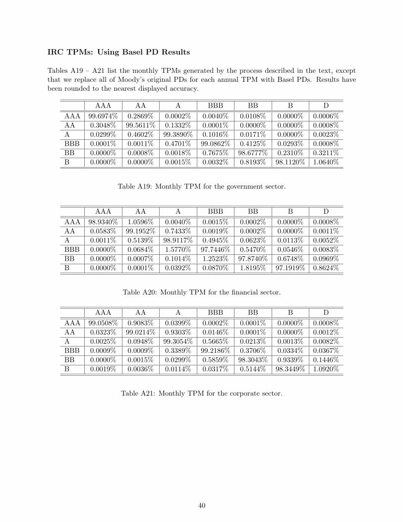
IRC TPMs: Using Basel PD Results
Tables A19 – A21 list the monthly TPMs generated by the process described in the text, exceptthat we replace all of Moody’s original PDs for each annual TPM with Basel PDs. Results havebeen rounded to the nearest displayed accuracy.
AAA AA A BBB BB B D
AAA 99.6974% 0.2869% 0.0002% 0.0040% 0.0108% 0.0000% 0.0006%
AA 0.3048% 99.5611% 0.1332% 0.0001% 0.0000% 0.0000% 0.0008%
A 0.0299% 0.4602% 99.3890% 0.1016% 0.0171% 0.0000% 0.0023%
BBB 0.0001% 0.0011% 0.4701% 99.0862% 0.4125% 0.0293% 0.0008%
BB 0.0000% 0.0008% 0.0018% 0.7675% 98.6777% 0.2310% 0.3211%
B 0.0000% 0.0000% 0.0015% 0.0032% 0.8193% 98.1120% 1.0640%
Table A19: Monthly TPM for the government sector.
AAA AA A BBB BB B D
AAA 98.9340% 1.0596% 0.0040% 0.0015% 0.0002% 0.0000% 0.0008%
AA 0.0583% 99.1952% 0.7433% 0.0019% 0.0002% 0.0000% 0.0011%
A 0.0011% 0.5139% 98.9117% 0.4945% 0.0623% 0.0113% 0.0052%
BBB 0.0000% 0.0684% 1.5770% 97.7446% 0.5470% 0.0546% 0.0083%
BB 0.0000% 0.0007% 0.1014% 1.2523% 97.8740% 0.6748% 0.0969%
B 0.0000% 0.0001% 0.0392% 0.0870% 1.8195% 97.1919% 0.8624%
Table A20: Monthly TPM for the financial sector.
AAA AA A BBB BB B D
AAA 99.0508% 0.9083% 0.0399% 0.0002% 0.0001% 0.0000% 0.0008%
AA 0.0323% 99.0214% 0.9303% 0.0146% 0.0001% 0.0000% 0.0012%
A 0.0025% 0.0948% 99.3054% 0.5665% 0.0213% 0.0013% 0.0082%
BBB 0.0009% 0.0009% 0.3389% 99.2186% 0.3706% 0.0334% 0.0367%
BB 0.0000% 0.0015% 0.0299% 0.5859% 98.3043% 0.9339% 0.1446%
B 0.0019% 0.0036% 0.0114% 0.0317% 0.5144% 98.3449% 1.0920%
Table A21: Monthly TPM for the corporate sector.
40

Tables A22 – A24 list the annual TPM generated by raising to the power of 12 the monthly TPMsof Tables A19 – A21. Results have been rounded to the nearest displayed accuracy.
AAA AA A BBB BB B D
AAA 96.4847% 3.3062% 0.0277% 0.0501% 0.1196% 0.0017% 0.0101%
AA 3.5147% 94.9526% 1.5086% 0.0101% 0.0039% 0.0001% 0.0101%
A 0.4297% 5.2187% 92.9775% 1.1292% 0.2099% 0.0046% 0.0304%
BBB 0.0111% 0.1462% 5.1903% 89.7869% 4.3971% 0.3560% 0.1123%
BB 0.0010% 0.0134% 0.2366% 8.1485% 85.5301% 2.3356% 3.7348%
B 0.0001% 0.0010% 0.0232% 0.3945% 8.2381% 79.6607% 11.6824%
Table A22: Annual TPM for the government sector generated by raising Table A19 to the powerof 12.
AAA AA A BBB BB B D
AAA 87.9685% 11.4770% 0.5152% 0.0249% 0.0036% 0.0008% 0.0100%
AA 0.6318% 91.0266% 8.0542% 0.2318% 0.0339% 0.0063% 0.0154%
A 0.0299% 5.5875% 88.3745% 4.9946% 0.7905% 0.1501% 0.0730%
BBB 0.0045% 1.1631% 15.8477% 76.8506% 5.2778% 0.6994% 0.1569%
BB 0.0007% 0.1045% 2.1290% 11.8976% 78.2821% 6.2129% 1.3732%
B 0.0001% 0.0233% 0.6203% 1.9861% 16.6802% 71.6796% 9.0103%
Table A23: Annual TPM for the financial sector generated by raising Table A20 to the power of12.
AAA AA A BBB BB B D
AAA 89.2035% 9.8026% 0.9485% 0.0334% 0.0019% 0.0002% 0.0101%
AA 0.3496% 88.9397% 10.1888% 0.4803% 0.0201% 0.0020% 0.0196%
A 0.0300% 1.0399% 92.1482% 6.2800% 0.3501% 0.0400% 0.1117%
BBB 0.0100% 0.0300% 3.7600% 91.2633% 3.9000% 0.5500% 0.4867%
BB 0.0015% 0.0201% 0.4400% 6.1697% 81.8392% 9.3295% 2.1999%
B 0.0200% 0.0400% 0.1400% 0.5100% 5.1400% 82.1200% 12.0300%
Table A24: Annual TPM for the corporate sector generated by raising Table A21 to the power of12.
41

IRC TPMs: Using Maximum Basel PD Results
Tables A25 – A27 list the monthly TPMs generated by the process described in the text, except thatwe replace all of Moody’s original PDs for each annual TPM with Basel maximum PDs. Resultshave been rounded to the nearest displayed accuracy.
AAA AA A BBB BB B D
AAA 99.6974% 0.2869% 0.0002% 0.0040% 0.0108% 0.0000% 0.0006%
AA 0.3048% 99.5611% 0.1332% 0.0001% 0.0000% 0.0000% 0.0008%
A 0.0299% 0.4602% 99.3881% 0.1016% 0.0171% 0.0000% 0.0030%
BBB 0.0001% 0.0011% 0.4706% 99.0820% 0.4147% 0.0296% 0.0020%
BB 0.0000% 0.0008% 0.0018% 0.7713% 98.6009% 0.2348% 0.3903%
B 0.0000% 0.0000% 0.0015% 0.0033% 0.8330% 97.9039% 1.2582%
Table A25: Monthly TPM for the government sector.
AAA AA A BBB BB B D
AAA 98.9339% 1.0596% 0.0040% 0.0015% 0.0002% 0.0000% 0.0008%
AA 0.0583% 99.1947% 0.7434% 0.0019% 0.0002% 0.0000% 0.0014%
A 0.0011% 0.5140% 98.9091% 0.4947% 0.0624% 0.0113% 0.0074%
BBB 0.0000% 0.0684% 1.5776% 97.7399% 0.5477% 0.0548% 0.0115%
BB 0.0000% 0.0007% 0.1014% 1.2539% 97.8551% 0.6789% 0.1099%
B 0.0000% 0.0001% 0.0393% 0.0870% 1.8306% 97.1013% 0.9417%
Table A26: Monthly TPM for the financial sector.
AAA AA A BBB BB B D
AAA 99.6974% 0.2869% 0.0002% 0.0040% 0.0108% 0.0000% 0.0006%
AA 0.3048% 99.5598% 0.1332% 0.0001% 0.0000% 0.0000% 0.0021%
A 0.0299% 0.4603% 99.3837% 0.1017% 0.0171% 0.0000% 0.0072%
BBB 0.0001% 0.0011% 0.4713% 99.0625% 0.4152% 0.0296% 0.0202%
BB 0.0000% 0.0008% 0.0018% 0.7722% 98.6008% 0.2348% 0.3895%
B 0.0000% 0.0000% 0.0015% 0.0033% 0.8330% 97.9039% 1.2583%
Table A27: Monthly TPM for the corporate sector.
42
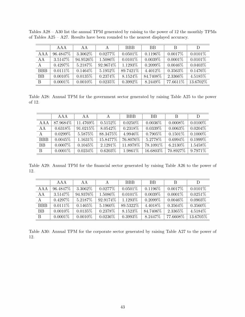
Tables A28 – A30 list the annual TPM generated by raising to the power of 12 the monthly TPMsof Tables A25 – A27. Results have been rounded to the nearest displayed accuracy.
AAA AA A BBB BB B D
AAA 96.4847% 3.3062% 0.0277% 0.0501% 0.1196% 0.0017% 0.0101%
AA 3.5147% 94.9526% 1.5086% 0.0101% 0.0039% 0.0001% 0.0101%
A 0.4297% 5.2187% 92.9674% 1.1293% 0.2099% 0.0046% 0.0403%
BBB 0.0111% 0.1464% 5.1952% 89.7421% 4.4012% 0.3563% 0.1476%
BB 0.0010% 0.0135% 0.2374% 8.1524% 84.7408% 2.3366% 4.5185%
B 0.0001% 0.0010% 0.0235% 0.3992% 8.2449% 77.6611% 13.6702%
Table A28: Annual TPM for the government sector generated by raising Table A25 to the powerof 12.
AAA AA A BBB BB B D
AAA 87.9684% 11.4769% 0.5152% 0.0250% 0.0036% 0.0008% 0.0100%
AA 0.6318% 91.0215% 8.0542% 0.2318% 0.0339% 0.0063% 0.0204%
A 0.0299% 5.5875% 88.3475% 4.9946% 0.7905% 0.1501% 0.1000%
BBB 0.0045% 1.1631% 15.8477% 76.8076% 5.2778% 0.6994% 0.1999%
BB 0.0007% 0.1045% 2.1291% 11.8978% 78.1091% 6.2130% 1.5458%
B 0.0001% 0.0234% 0.6203% 1.9861% 16.6803% 70.8927% 9.7971%
Table A29: Annual TPM for the financial sector generated by raising Table A26 to the power of12.
AAA AA A BBB BB B D
AAA 96.4847% 3.3062% 0.0277% 0.0501% 0.1196% 0.0017% 0.0101%
AA 3.5147% 94.9376% 1.5086% 0.0101% 0.0039% 0.0001% 0.0251%
A 0.4297% 5.2187% 92.9174% 1.1293% 0.2099% 0.0046% 0.0903%
BBB 0.0111% 0.1465% 5.1960% 89.5322% 4.4018% 0.3564% 0.3560%
BB 0.0010% 0.0135% 0.2378% 8.1523% 84.7406% 2.3365% 4.5184%
B 0.0001% 0.0010% 0.0236% 0.3993% 8.2447% 77.6608% 13.6705%
Table A30: Annual TPM for the corporate sector generated by raising Table A27 to the power of12.
43

References
[1] Basel Committee on Banking Supervision, Guidelines for computing capital for incrementalrisk in the trading book, Bank for International Settlements, July 2009.
[2] Basel Committee on Banking Supervision, International Convergence of Capital Measurementand Capital Standards - A Revised Framework Comprehensive Version, Bank for InternationalSettlements, June 2006.
[3] Elena Duggar et al., Sovereign Default and Recovery Rates, 1983-2008, Moody’s InvestorsService, Global Corporate Finance, Special Comment, 17 March 2009.
[4] Kenneth Emery et al., Corporate Default and Recovery Rates, 1920-2009, Moody’s InvestorsService, Global Corporate Finance, Special Comment, 10 February 2010.
[5] Ozgur B. Kan, Moody’s Credit Risk Calculator: User Manual, Moody’s Investors Service,September 2007, http : //www.moodys.com/cust/content/Content.ashx?source = StaticContent/Free Pages/Products and Services/Downloadable Files/sp1033 risk calculator4 web.pdf
[6] P. J. Schonbucher, Credit Derivatives Pricing Models: Models, Pricing and Implementation,John Wiley & Sons, June 2003.
[7] D. Lando, Three Essays on Contingent Claims Pricing, Ph.D. Thesis, Graduate School ofManagement, Cornell University, 1994.
[8] R. A. Jarrow, D. Lando and S. M. Turnbull, A Markov Model for the Term Structure of CreditRisk Spreads, The Review of Financial Studies, Summer 1997 Vol. 10, No. 2, pp. 481-523.
[9] M. Kijima and K. Komoribayashi, A Markov Chain Model for Valuing Credit Risk Derivatives,The Journal of Derivatives, Fall 1998, Vol. 6, No. 1, pp. 97-108.
[10] D. Lando, Some Elements of Rating-based Credit Risk Modeling. In N. Jegadeesh and B.Tuckman (Eds.), Advanced Fixed-Income Valuation Tools, John Wiley & Sons, Chichester, pp.193-215.
[11] Alexander Kreinin and Marina Sidelnikova, Regularization Algorithms for Transition Matrices,Algo Research Quarterly, Vol. 4, Nos. 1/2, March/June 2001.
[12] M. Araten and L. Angbazo, Roots of transition matrices: Application to settlement risk. ChaseManhattan Bank, 1997, Practical Paper.
[13] W. Stromquist, Roots of Transition Matrices, Daniel H. Wagner Associates, April 24, 1996,Practical Paper.
[14] A. Andersson and P. Vanini, Credit Migration Risk Modelling, National Centre of Competencein Research Financial Valuation and Risk Management Working Paper No. 538, June 2009.
44


![The Probability that a Random Real Gaussian Matrix has k Real …edelman/publications/probability... · 2018-12-28 · circular law [14], which states that if the elements of a random](https://img.dokumen.tips/doc/110x75/5e95af3b18159d4b997eee49/the-probability-that-a-random-real-gaussian-matrix-has-k-real-edelmanpublicationsprobability.jpg)