Transport in Porous Media (2019) 126:743–777https://doi.org/10.1007/s11242-018-1194-z

Transient and Pseudo-Steady-State Inflow PerformanceRelationships for Multiphase Flow in FracturedUnconventional Reservoirs

Salam Al-Rbeawi1

Received: 6 June 2018 / Accepted: 31 October 2018 / Published online: 8 November 2018© Springer Nature B.V. 2018

AbstractThe objective of this paper is developing newmethodology for constructing the inflow perfor-mance relationships (IPRs) of unconventional reservoirs experiencing multiphase flow. Themotivation is eliminating the uncertainties of using single-phase flow IPRs and approachingrealistic representation and simulation to reservoir pressure–flow rate relationships through-out the entire life of production. Several analytical models for the pressure drop and declinerate as wells productivity index of two wellbore conditions, constant Sandface flow rateand constant wellbore pressure, are presented in this study. Several deterministic models arealso proposed in this study for multiphase reservoir total mobility and compressibility usingmulti-regression analysis of PVT data and relative permeability curves of different reservoirfluids. These deterministic models are coupled with the analytical models of pressure drop,decline rate, and productivity index to construct the pressure–flow rate relationships (IPRs)during transient and pseudo-steady-state production time. Transient IPRs are generated forearly-time hydraulic fracture linear flow regime and intermediate-time bilinear and trilinearflow regimes, while steady-state IPRs are generated for pseudo-steady-state flow regime incase of constant Sandface flow rate and boundary-dominated flow regime in case of constantwellbore pressure. The outcomes of this study are as follows: (1) introducing the impactof multiphase flow to the IPRs of unconventional reservoirs; (2) developing deterministicmodels for reservoir total mobility and compressibility using multi-regression analysis ofPVT data and relative permeability curves; (3) developing analytical models for differentflow regimes that could be developed during the entire production life of reservoirs; (4)predicting transient and steady-state IPRs of multiphase flow for different wellbore condi-tions. The study has pointed out: (1) Multiphase flow conditions have significant impact onreservoir IPRs. (2)Multiphase reservoir total mobility and compressibility exhibit significantchange with reservoir pressure. (3) Constant Sandface flow rate may demonstrate IPR betterthan constant wellbore pressure. (4) Late production time is not affected by multiphase flowconditions similar to transient state flow at early and intermediate production time.

B Salam Al-Rbeawisalam@metu.edu.tr

1 METU-Northern Cyprus Campus, Turkey

123

744 S. Al-Rbeawi

Keywords Multiphase flow · Unconventional reservoirs · Hydraulic fracturing · Fracturedformations · Inflow performance relationship

List of symbols

Bg Gas formation volume factorB ′g Derivative of gas formation volume factor

Bo Oil formation volume factorB ′o Derivative of oil formation volume factor

Bt Total formation volume factorBw Water formation volume factorB ′w Derivative of water formation volume factor

cAFq Shape factor for constant Sandface flow rate approachcAFP Shape factor for constant wellbore pressure approachcF Reservoir fluid total compressibility, psi−1

cg Gas - phase compressibility, psi−1

co Oil - phase compressibility, psi−1

cw Water - phase compressibility, psi−1

(ct)mp Multiphase reservoir total compressibility, psi−1

FCD Hydraulic fracture conductivity, dimensionlessJDP Productivity index of constant wellbore pressure, dimensionlessJDq Productivity index of constant Sandface flow rate, dimensionlessh Formation thickness, ftki Induced matrix permeability, mdkm Matrix permeability, md(k/μ)mp Multiphase reservoir total mobility, md/cpP Pressure, psiPb Bubble point pressure, psi�Pwf Wellbore pressure drop, psiPD Pressure drop, dimensionlessPDi Initial reservoir pressure, dimensionlessPwD Wellbore pressure drop, dimensionlesstDx P ′

D Pressure derivative, dimensionlessqD Sandface flow rate, dimensionlessqo oil flow rate, STB/dayqt Total flow rate, bbl/dayqw water flow rate, STB/dayqsc Gas flow rate,MScf/dayRs Solution gas − oil ratioR′s Derivative of solution gas − oil ratio

Rsb Solution gas − oil ratio at bubble point pressureRsw Solution gas − water ratioR′sw Derivative of solution gas − water ratio

s Laplace operatorSg Gas saturationSo Oil saturationSw Water saturation

123

Transient and Pseudo-Steady-State Inflow Performance… 745

T Reservoir temperaturet Time, htD Time, dimensionlessμg Gas - phase viscosity, cpμo Oil - phase viscosity, cpμw Water - phase viscosity, cpwf Hydraulic fracture − half - length, ftxe Reservoir boundary, ftxf Hydraulic fracture width, ftye Reservoir boundary, ftω Storativity∅ Porosityλ Interporosity flow coefficient

1 Introduction

The literature review of the two topics of interest in this paper is covered briefly. The first is thepressure behavior, decline rate, and productivity index of hydraulically fractured reservoirs,while the second focuses on the attempts of assembling the impact of multiphase flow withreservoir performance models. To avoid the excessive length of the manuscript, the literaturereview of the first part will not be discussed in details, while the second will be the focus ofthe literature review.

In the last couple decades, hydraulic fracturing stimulation technique has boosted updeveloping economically unconventional resources in spite of the great challenges. Improvingthe ultralow permeability of these resources and creating high-conductivity flow paths in theporous media are the key points in the process. As a matter of fact, starting from the firstsucceed of this technique and later on until the moment, a lot of researches in different topicsand disciplines have been conducted and presented in the petroleum industry literature.Within the scope of this paper, topics such as pressure transient analysis (PTA), rate transitanalysis (RTA), and productivity index of hydraulically fractured reservoirs are very wellcovered. At early 1960s, the physical meaning of dimensionless fracture conductivity wasexplained by Prats and Levine (1963) as the ratio of the ability of hydraulic fractures totransmit reservoir fluid to the wellbore, while 1970s have witnessed serious attempts toformulate pressure behavior and decline rate of fractured formations conducted byGringartenand Ramey (1973), Gringarten et al. (1974), Cinco-Ley (1974), Holditch and Morse (1976),Raghavan et al. (1978), Cinco-Ley et al. (1975), Cinco et al. (1978), andAgarwal et al. (1979).These attempts have continued during the 1980s and 1990s by Cinco-Ley and Samaniego(1981), Bennett et al. (1986), Camacho et al. (1987), Ozkan (1988), Guppy et al. (1988),Ozkan and Raghavan (1991a, b), Soliman et al. (1990), Kuchuk (1990), Larsen and Hegre(1994), Raghavan et al. (1997), El-Banbi (1998), andWan andAziz (1999). The later 20 yearshave witnessed a great attention given to rate transient analysis (RTA) as well as pressuretransient analysis (PTA). Because of the ultralow permeability in unconventional reservoirs,pressure pulse may need a very long time to reach the boundary and thereby pseudo-steady-state or boundary-dominated flow regime might not be observed. Therefore, RTA has beenused confidentially as an excellent tool for unconventional reservoir characterization morethan PTA. This has come out with a lot of models that describe decline rate with productiontime such as those proposed by Hagoort (2003), Levitan (2005), Ilk et al. (2006), Ibrahim

123

746 S. Al-Rbeawi

and Wattenbarger (2006), Camacho et al. (2008), Bello (2008), Izadi and Yildiz (2009), andCipolla (2009). Very recently, the two topics (RTA and PTA) have been supported by moreresearch papers presented by Ozkan et al. (2011), Brown et al. (2011), Duong (2011), Chenand Jones (2012), Nobakht et al. (2012), Torcuk et al. (2013), Fuentes-Cruz et al. (2014),Luo et al. (2014), Shahamat et al. (2015), Fuentes-Cruz and Valko (2015), Behmanesh et al.(2015, 2018), and Kanfar and Clarkson (2018).

In the above-mentioned studies, single-phase flow is assumed as the dominant flow patternin the porous media. This assumption might have led to misleading results for reservoirsthat undergo multiphase flow conditions. In conventional reservoirs, single-phase flow isthe common flow pattern in oil reservoirs with pressure greater than bubble point pressure.Single-phase flow is also the dominant flow pattern for natural dry gas reservoir and to someextent wet gas reservoirs. While in oil reservoirs where the pressure could drawdown thebubble point pressure, volatile oil reservoirs, and retrograde-condensate or near critical gas-condensate reservoirs, multiphase flow is the norm. Unconventional reservoirs may not havean exemption from the above-mentioned classification even though most shale layers areconsidered gas-producing plays. However, North Dakota Bakken formation and Texas EagleFord formation in the USA are two examples of ultralow permeability porous media wheremultiphase flow (black oil +gas) is the overwhelming flow pattern (Uzun et al. 2016).

No doubt, dealing with single-phase flow is much easier than with multiphase flow interms of physical properties of reservoir fluids and petrophysical properties of porous media.Reservoir modeling for fluid flow and pressure distribution in drainage areas that undergosingle-phase (oil or gas) flow can be accomplished either analytically or numerically witha consideration given to the absolute permeability of the porous media and total reservoircompressibility only. This would not be the case for multiphase flow where the consider-ations should be focused on relative permeability and saturation of each phase as well asthe continuously changing reservoir fluid properties such as density, viscosity, formationvolume factor, gas solubility, and compressibility. The problem could be more complicatedconsidering that associated linear behavior of most reservoir rock and fluid properties insingle-phase flow may not be applicable for multiphase flow. Nonlinear scheme (Tabatabaieand Pooladi-Darvish 2017) demonstrates most of the pressure- and time-dependent reservoirfluid properties as well as the changes in relative permeabilities with saturation that in turncould change with time and reservoir pressure.

Not until recently, multiphase flow has been given the attention in petroleum industry. Themathematical treatment proposed by Muskat and Meres (1936) for fluid flow in hydrocarbonreservoirs was considered by Perrine (1956) for multiphase flow and 3 years later Martin(1959) introduced a simplified equation for multiphase flow in gas drive reservoirs whereinrelative permeability of reservoir fluid phases and their physical properties were considered.This simplified equationwasobtainedby the assumptionof neglecting the pressure–saturationgradient as their vector products are small compared with the magnitude of pressure vectoror saturation vector. Martin and James (1963) applied the proposed model by Martin (1959)for pressure transient analysis of two-phase radial flow considering constant pressure andno flow at the outer boundary. Because of the difficulties that governed utilizing multiphaseflow in well test analysis, very limited attempts were conducted after the one proposed byMartin and James (1963). Chu et al. (1986) reconsidered two-phase flow problem in pressuretransient applications. In that study, the primary concern was the saturation gradient and therelative permeability of each phase of reservoir fluid. The conceptual approach presentedby Martin (1959) was adopted by Raghavan (1976, 1989) for the applications of well testanalysis for a well producing from solution gas driven at constant surface production rate.At the same time, Fraim andWattenbarger (1988) used the basic model presented by Muskat

123

Transient and Pseudo-Steady-State Inflow Performance… 747

(1937) for the applications of decline curve analysis considering multiphase flow in porousmedia. They concentrated on the effect of saturation gradient on rate–time profile as reservoirpressure moves down the bubble point pressure.

Ayan and Lee (1988) stated that even though the approaches presented by Perrine (1956)and Martin (1959) are simple, they could yield misleading results under some circumstancesas a consequence of the inherently assumptions in those two approaches including the non-uniform distribution of saturation and compressibility in the porous media. For this reason,Boe et al. (1989) believed that multiphase flow effect can be adapted to the liquid model solu-tions if totalmobility and compressibility are used and pseudo-pressure function is developed.However, creating pseudo-pressure function needs very well-defined relationship betweenoil saturation and pressure that in turn needs the assumptions followed by Perrine (1956) andMartin (1963). For more easiness and less assumptions, Al-Khalifa et al. (1989) suggestedusing pressure square approach for multiphase flow instead of pseudo-pressure approach.They stated that the rate normalization using pressure square approach may yield reasonableestimates for the individual phase permeability and thereby accurate total mobility. Morethan 10 years later, Kamal and Pan (2010, 2011) demonstrated the applicability of pressuretransient analysis for reservoir characterization under multiphase flow conditions. Recently,Li et al. (2017) proposed newmethod for construction gas–water two-phase steady-state flowproductivity of fractured horizontal wells depleting tight gas reservoirs.

Unfortunately, despite the great attention given to multiphase flow in porous media, theabove-mentioned attempts have not reached to robust techniques that rigorously includedthe impact of multiphase flow on reservoir performance. This could be explained by thedifficulties that governed the proposed models for predicting the variances of physical andpetrophysical properties such as saturation, viscosity, density, formation volume factor, andrelative permeability with time. Therefore, most of the proposed models for the IPR assumedsingle-phase flow either oil or gas. However, from time to time, two-phase flow or multiphaseflow IPRs have been suggested by several authors. Gallice and Wiggins (2004) investigatedthe IPRs for predicting pressure/production behavior of reservoirs dominated by two-phaseflow. Ten years before, Wiggins (1994) introduced a study for three-phase flow generalizedIPR, while Camacho andRaghavan (1989) used numerical model for examining the influenceof reservoir pressure on the IPR for reservoirs producing under solution gas derive.

In this paper, the IPR of unconventional reservoirs consideringmultiphase flow conditionsin the porous media is introduced. Early production time transient state flow IPR and lateproduction time pseudo-state IPR are considered for constant Sandface flow rate and constantwellbore pressure. Several deterministicmodels for reservoir totalmobility and compressibil-ity are generated from PVT data and relative permeability curves. The analytical models ofthe flow regimes, developed in bounded hydraulically fractured unconventional reservoirs,are included the impact of multiphase flow condition and used to generate transient andpseudo-steady-state IPRs.

2 Multiphase Reservoir Total Compressibility (ct)mp andMobility(k�

)mp

When the pressure in oil reservoirs declines less than bubble point pressure, free gas phaseis developed as well as liquid phase. Therefore, two-phase flow (oil and gas) or even multi-phase flow (oil, gas, and water) in case of water production is expected to occur in porousmedia. Therefore, the assumption for developing multiphase reservoir total compressibility

123

748 S. Al-Rbeawi

and mobility models is (P < Pb). For multiphase flow conditions, reservoir total compress-ibility depends on reservoir fluids’ saturation that in turn depends on reservoir pressure. Themathematical models for this compressibility can be written as:

(ct)mp � cf + Soco + Sgcg + Swcw. (1)

It is well known that formation compressibility (cf) may not significantly change withpressure, while reservoir fluid compressibilities, oil compressibility (co), gas compressibility(cg), and water compressibility (cw), are pressure-variant parameters. Several models wereintroduced in the literature for the changes in the three-phase reservoir fluid compressibilities.The following model was presented by Martin (1959), Raghvan (1989), and Tabatabaie andPooladi-Darvish (2017) for reservoir fluid total compressibility:

cF � So f (Co) + Sw f (Cw) + Sg f(Cg

), (2)

where

f (Co) � BgR′s

Bo− B ′

o

Bo, (3)

f (Cw) � BgR′sw

Bw− B ′

w

Bw, (4)

f(Cg

) � − B ′g

Bg. (5)

It can be clearly understood that the functions in Eqs. (3)–(5) are pressure-dependentfunctions since all parameters included in these functions such as oil, water, and gas forma-tion volume factors as well as the gas solubility in oil and water are functions of pressure.Therefore, reservoir fluid total compressibility (cF), given by Eq. (2), is expected to bepressure-dependent parameter. To develop deterministic models for these parameters, thethree situations (oil So, gas Sg, and water Sw) in Eq. (2) should be determined first. For thispurpose, it is required to calculate oil and water saturation derivatives with pressure. In thisstudy, the following two models (Martin 1959) are used to calculate oil and water saturationderivatives with pressure:

dS0dP

� SoB ′o

Bo+kro/μ0(kμ

)

mp

cF, (6)

dSwdP

� SwB′w

Bw+krw/μw(

kμ

)

mp

cF. (7)

To solve Eqs. (6) and (7), reservoir total mobility(kμ

)

mpshould be calculated as well as

oil, gas, and water saturation for each pressure step. Therefore, relative permeabilities of thethree phases have to be estimated. From oil–water system using water saturation, relativepermeability of water (krw) can be estimated while relative permeability of gas phase

(krg

)is

predicted from gas–water system knowing gas saturation. These two relative permeabilitiesare used to calculate the relative permeability of oil phase (kro) by several models proposedin the literature such as Stone I and II models (Stone 1970, 1973) or it could be determined

123

Transient and Pseudo-Steady-State Inflow Performance… 749

Fig. 1 Oil relative permeability behavior with water and gas saturations

graphically as shown in Fig. 1 using the two saturations of oil and water calculated by Stones’models. Mathematically, multiphase reservoir total mobility is calculated by:

(k

μ

)

mp� kro

μo+krgμg

+krwμw

. (8)

For better understanding the methodology proposed in this study for calculating reservoirtotal mobility and compressibility, a set of PVT data given in Table 1, taken from Boeet al. (1989), is used. Reservoir and fluid properties are given in Table 2. Because neitherwater formation volume factor (Bw) nor solution gas–water ratio is given in Table 1, thesetwo parameters are calculated using the following two models for reservoir temperature(T � 200

◦F)(Lee and Wattenbarger 1996):

Bw � 1.039 − 4.1 ∗ 10−6P − 7.4 ∗ 10−9P2, (9)

Rsw � 0.7883 + 2.1683 ∗ 10−3P − 0.93 ∗ 10−7P2, (10)

while formation water viscosity is calculated by:

μw � μ1

[0.9993 + 4.0295 ∗ 10−5P + 3.1062 ∗ 10−9P2

], (11)

where (μ1) formation water viscosity at atmospheric pressure and reservoir temperature andcalculated by:

μ1 � AT B , (12)

where (A) and (B) are two constants and determined by several models presented in the liter-ature based on formation water solid content or reservoir temperature (Lee andWattenbarger1996).

The calculated properties of formation water are given in Table 3.

123

750 S. Al-Rbeawi

Table 1 A set of PVT data (Boe et al. 1989)

P, psi Bo bbl/STB BGo bbl/SCF RS SCF/STB μo, cp μg, cp

5705 1.806 0.000596 1499.00 0.298 0.0298

5633 1.791 0.000600 1470.38 0.3 0.0295

5204 1.702 0.000625 1305.56 0.317 0.0281

4703 1.605 0.000661 1127.45 0.348 0.0263

4202 1.516 0.000709 963.48 0.391 0.0246

3700 1.434 0.000775 812.57 0.446 0.0228

3200 1.36 0.000870 673.78 0.515 0.021

2770 1.302 0.000991 563.79 0.587 0.0195

2340 1.249 0.001172 461.53 0.671 0.0181

1911 1.202 0.001455 366.52 0.768 0.0166

1482 1.159 0.001929 278.24 0.881 0.0152

1052 1.121 0.002826 196.10 1.011 0.0138

623 1.088 0.004998 119.14 1.164 0.0125

193 1.058 0.016881 44.29 1.35 0.0113

Table 2 Reservoir physical andpetrophysical properties (Boeet al. 1989)

Porosity, ∅ 30%

Permeability, k 10 md

Intial reservoir pressure, Pi 5705 psi

Bubble point pressure, Pb 5705 psi

Initial water saturation, Swi 30%

Initial gas saturation, Sgi 0.0

Wellbore radius, rw 0.33 ft

Reservoir radius, re 656 ft

Formation thickness, h 15.6ft

Gas specific gravity, γg 0.75

Reservoir temperature, T 200 °F

Crude oil API 35

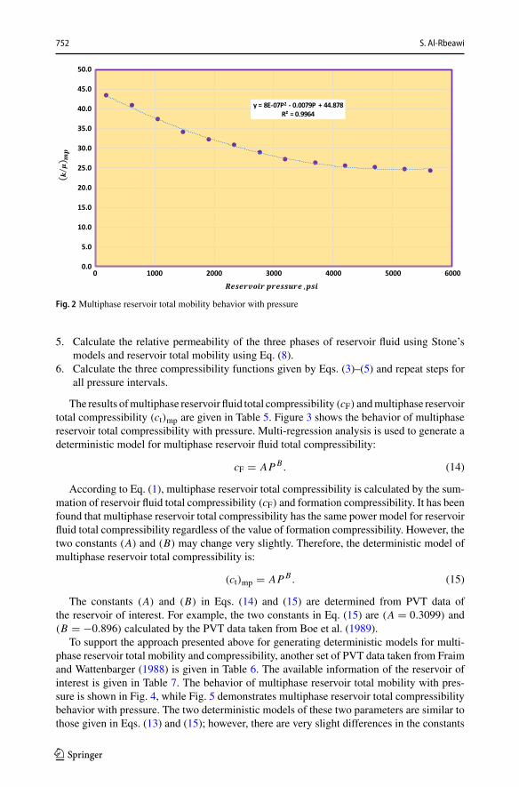
The calculated relative permeabilities of the three phases of reservoir fluids are used tocalculate multiphase reservoir total mobility, given by Eq. (8). The results are given in Table 4and plotted in Fig. 2. Multi-regression analysis is used to generate a deterministic model formultiphase reservoir total mobility with reservoir pressure. This model is:

(k

μ

)

mp� AP2 + BP + C, (13)

where the constants(A � 8 ∗ 10−7

), (B � −0.0079), and (C � 44.9) are determined by the

PVT data of the reservoir of interest.To calculate reservoir total compressibility (ct)mp, reservoir fluid total compressibility

(cF ) should be calculated first. The following procedures illustrate the methodology used forcalculating reservoir total compressibility.

123

Transient and Pseudo-Steady-State Inflow Performance… 751

Table 3 Calculated formationwater properties

P, psi Rsw SCF/STB μw, cp Bw bbl/STB

5705 10.132 1.3304 1.0162

5633 10.051 1.3249 1.0170

5204 9.554 1.2932 1.0210

4703 8.929 1.2576 1.0250

4202 8.257 1.2236 1.0282

3700 7.538 1.1910 1.0308

3200 6.775 1.1602 1.0329

2770 6.081 1.1349 1.0343

2340 5.353 1.1107 1.0355

1911 4.592 1.0877 1.0365

1482 3.797 1.0659 1.0373

1052 2.966 1.0452 1.0379

623 2.103 1.0257 1.0384

193 1.203 1.0073 1.0388

Table 4 Reservoir total mobility results

P, psi kro krg krwo kro/o krg/g krw/w (k/μ)mp

5705 0.805 0 0 2.701 0.000 0.000 2.701

5633 0.802 0.6383 0.02 2.673 21.637 0.015 24.326

5204 0.751 0.6253 0.05 2.369 22.253 0.039 24.660

4703 0.71 0.606 0.08 2.040 23.042 0.064 25.146

4202 0.615 0.5885 0.1 1.573 23.923 0.082 25.577

3700 0.554 0.5681 0.11 1.242 24.917 0.092 26.251

3200 0.505 0.547 0.13 0.981 26.048 0.112 27.140

2770 0.462 0.5453 0.14 0.787 27.964 0.123 28.875

2340 0.421 0.5437 0.15 0.627 30.039 0.135 30.801

1911 0.382 0.5242 0.16 0.497 31.578 0.147 32.223

1482 0.351 0.5094 0.17 0.398 33.513 0.159 34.071

1052 0.331 0.508 0.18 0.327 36.812 0.172 37.311

623 0.302 0.5052 0.19 0.259 40.416 0.185 40.861

193 0.252 0.4856 0.2 0.187 42.973 0.199 43.359

1. At the bubble point pressure, the three compressibility functions given by Eqs. (3)–(5)are calculated as well as reservoir total mobility.

2. Using initial saturations at bubble point pressure, reservoir fluid total compressibility iscalculated using Eq. (2) andmultiphase reservoir total compressibility is calculated usingEq. (1).

3. Calculate oil and water saturation derivatives given by Eqs. (6) and (7) for the secondpressure interval.

4. Calculate oil and water saturation for the new pressure interval. Gas saturation is calcu-lated by

(Sg � 1 − Sw − So

).

123

752 S. Al-Rbeawi

y = 8E-07P2 - 0.0079P + 44.878R² = 0.9964

0.0

5.0

10.0

15.0

20.0

25.0

30.0

35.0

40.0

45.0

50.0

0 1000 2000 3000 4000 5000 6000

Fig. 2 Multiphase reservoir total mobility behavior with pressure

5. Calculate the relative permeability of the three phases of reservoir fluid using Stone’smodels and reservoir total mobility using Eq. (8).

6. Calculate the three compressibility functions given by Eqs. (3)–(5) and repeat steps forall pressure intervals.

The results ofmultiphase reservoir fluid total compressibility (cF) andmultiphase reservoirtotal compressibility (ct)mp are given in Table 5. Figure 3 shows the behavior of multiphasereservoir total compressibility with pressure. Multi-regression analysis is used to generate adeterministic model for multiphase reservoir fluid total compressibility:

cF � APB . (14)

According to Eq. (1), multiphase reservoir total compressibility is calculated by the sum-mation of reservoir fluid total compressibility (cF) and formation compressibility. It has beenfound that multiphase reservoir total compressibility has the same power model for reservoirfluid total compressibility regardless of the value of formation compressibility. However, thetwo constants (A) and (B) may change very slightly. Therefore, the deterministic model ofmultiphase reservoir total compressibility is:

(ct)mp � APB . (15)

The constants (A) and (B) in Eqs. (14) and (15) are determined from PVT data ofthe reservoir of interest. For example, the two constants in Eq. (15) are (A � 0.3099) and(B � −0.896) calculated by the PVT data taken from Boe et al. (1989).

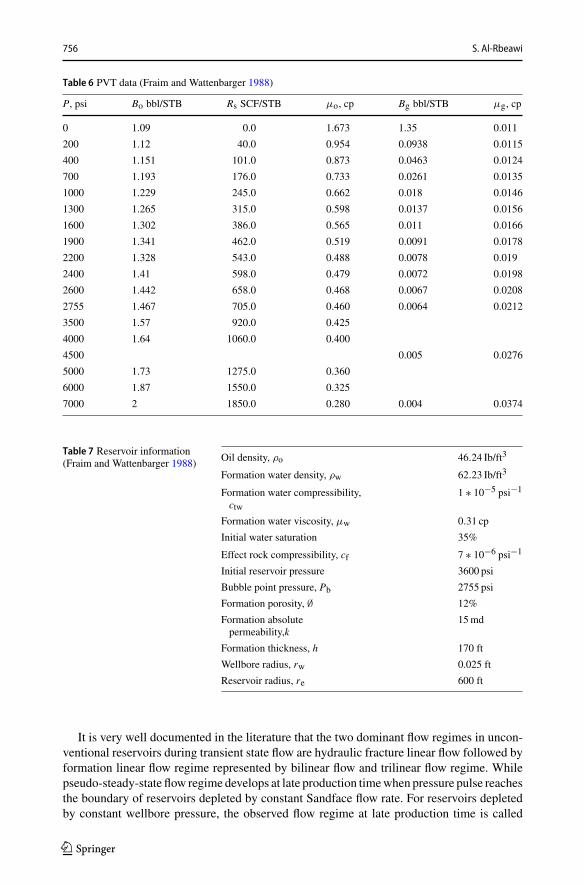
To support the approach presented above for generating deterministic models for multi-phase reservoir total mobility and compressibility, another set of PVT data taken from Fraimand Wattenbarger (1988) is given in Table 6. The available information of the reservoir ofinterest is given in Table 7. The behavior of multiphase reservoir total mobility with pres-sure is shown in Fig. 4, while Fig. 5 demonstrates multiphase reservoir total compressibilitybehavior with pressure. The two deterministic models of these two parameters are similar tothose given in Eqs. (13) and (15); however, there are very slight differences in the constants

123

Transient and Pseudo-Steady-State Inflow Performance… 753

Table5Multip

hase

reservoirflu

idtotalcom

pressibilityandreservoirtotalcom

pressibilityresults

P,p

sif(Co)

f(Cw)

f(Cg)

k ro

k rg

k rw

dSo/dP

dSw/dP

5705

2.84

217E

−05

0.00

0115

124

0.00

0151

997

0.80

50

00.00

0118

04−3

.428

18E−0

5

5633

2.92

528E

−05

0.00

0112

842

0.00

0154

937

0.80

20.63

830.02

6.88

79E−0

5−3

.383

65E−0

5

5204

3.47

861E

−05

0.00

0100

175

0.00

0174

279

0.75

10.62

530.05

6.55

41E−0

5−3

.137

14E−0

5

4703

4.25

923E

−05

8.70

976E

−05

0.00

0201

683

0.71

0.60

60.08

6.16

18E−0

5−2

.848

47E−0

5

4202

5.24

708E

−05

7.54

926E

−05

0.00

0235

598

0.61

50.58

850.1

5.72

3E−0

5−2

.558

59E−0

5

3700

6.55

027E

−05

6.50

462E

−05

0.00

0277

965

0.55

40.56

810.11

5.30

49E−0

5−2

.267

47E−0

5

3200

8.34

266E

−05

5.56

038E

−05

0.00

0330

732

0.50

50.54

70.13

4.89

24E−0

5−1

.971

31E−0

5

2770

0.00

0104

926

4.81

375E

−05

0.00

0387

535

0.46

20.54

530.14

4.52

84E−0

5−1

.715

86E−0

5

2340

0.00

0135

407

4.12

212E

−05

0.00

0459

398

0.42

10.54

370.15

4.16

88E−0

5−1

.456

72E−0

5

1911

0.00

0180

454

3.48

757E

−05

0.00

0554

911

0.38

20.52

420.16

3.81

75E−0

5−1

.191

11E−0

5

1482

0.00

0251

826

2.91

979E

−05

0.00

0695

811

0.35

10.50

940.17

3.47

74E−0

5−9

.159

98E−0

6

1052

0.00

0378

684

2.45

917E

−05

0.00

0942

774

0.33

10.50

80.18

3.15

12E−0

5−6

.242

59E−0

6

623

0.00

0669

479

2.28

134E

−05

0.00

1519

608

0.30

20.50

520.19

2.86

71E−0

5−2

.773

17E−0

6

193

0.00

2199

146

4.13

836E

−05

0.00

4688

456

0.25

20.48

560.2

2.92

37E−0

55.23

169E

−06

S oS g

S wk ro/μ

ok rg/μ

gk rw/μ

wc F

(ct)mp

0.7

00.3

2.70

1342

282

00

5.44

324E

−05

6.44

324E

−05

0.69

1501

330.00

6030

382

0.30

2468

288

2.67

3333

333

21.637

2881

40.01

5094

982

5.52

937E

−05

6.52

937E

−05

0.66

1952

103

0.02

1063

747

0.31

6984

152.36

9085

174

22.252

6690

40.03

8663

299

5.84

516E

−05

6.84

516E

−05

0.62

9116

026

0.03

8182

736

0.33

2701

238

2.04

0229

885

23.041

8251

0.06

3612

677

6.34

737E

−05

7.34

737E

−05

123

754 S. Al-Rbeawi

Table5continued

S oS g

S wk ro/μ

ok rg/μ

gk rw/μ

wc F

(ct)mp

0.59

8245

605

0.05

4782

346

0.34

6972

049

1.57

2890

026

23.922

7642

30.08

1728

382

7.04

909E

−05

8.04

909E

−05

0.56

9516

207

0.07

0667

602

0.35

9816

191.24

2152

466

24.916

6666

70.09

2358

169

8.03

526E

−05

9.03

526E

−05

0.54

2991

711

0.08

5854

733

0.37

1153

555

0.98

0582

524

26.047

6190

50.11

2054

332

9.43

324E

−05

0.00

0104

332

0.52

1954

508

0.09

8415

291

0.37

9630

201

0.78

7052

811

27.964

1025

60.12

3364

244

0.00

0111

180.00

0121

18

0.50

2482

397

0.11

0509

214

0.38

7008

388

0.62

7421

759

30.038

6740

30.13

5050

138

0.00

0134

760.00

0144

76

0.48

4598

046

0.12

2144

237

0.39

3257

717

0.49

7395

833

31.578

3132

50.14

7092

982

0.00

0168

942

0.00

0178

942

0.46

8221

156

0.13

3411

276

0.39

8367

568

0.39

8410

897

33.513

1578

90.15

9483

736

0.00

0222

371

0.00

0232

371

0.45

3268

406

0.14

4425

233

0.40

2306

361

0.32

7398

615

36.811

5942

0.17

2211

233

0.00

0317

699

0.00

0327

699

0.43

9749

641

0.15

5265

928

0.40

4984

431

0.25

9450

172

40.416

0.18

5237

653

0.00

0539

586

0.00

0549

586

0.42

7420

959

0.16

6402

147

0.40

6176

894

0.18

6666

667

42.973

4513

30.19

8552

032

0.00

1736

939

0.00

1746

939

123

Transient and Pseudo-Steady-State Inflow Performance… 755

y = 0.3099P-0.986

R² = 0.9991

0.0000

0.0002

0.0004

0.0006

0.0008

0.0010

0 1000 2000 3000 4000 5000 6000

Fig. 3 Multiphase reservoir total compressibility behavior with pressure

of these two models obtained by analyzing PVT data given by Boe et al. (1989) and PVTdata given by Fraim and Wattenbarger (1988). The differences of the constants in these twomodels come from the differences in the two reservoir fluid properties and the differencesin reservoir conditions. Therefore, for more accuracy to the proposed approach used in thismanuscript, more PVT data sets can be used for developing different multiphase reservoirtotal compressibility and mobility models. Accordingly, the average values of the parametersincluded in these two models can be calculated and used for generating single and unique setof the two models of compressibility and mobility.

In the next sections, reservoir total mobility and compressibility, calculated by Eqs. (13)and (15), respectively, will be used in predicting transient and pseudo-steady-state IPR forunconventional reservoirs.

3 Transient Inflow Performance Relationship

Unconventional reservoirs are characterized by dominating transient state flow for a verylong production time. The reason for that refers to a very slow transferring rate of pressurepulse in the porous media due to ultralow permeability. Accordingly, the conclusions thatmost of the production comes from transient state flow and pseudo-steady-state flowmay notbe reached are not unrealistic. Unlike pseudo-steady-state flow, transient state flow is knownby varied productivity index. Because of that and considering multiphase flow conditions,conventional IPRmodels (Vogel 1968; Standing 1971; Fetkovich 1973;Wiggins 1994; Golanand Whitson 1995) may give misleading results. Therefore, new methodology is proposedin this study for pressure–flow rate relationships of unconventional reservoirs undergoingmultiphase flow. The new methodology states that the IPRs of this type of reservoirs arenot constant. They are changed with production time and the dominant flow regime in theporous media. Accordingly, different IPRs should be constructed for different flow regimesand production time.

123

756 S. Al-Rbeawi

Table 6 PVT data (Fraim and Wattenbarger 1988)

P, psi Bo bbl/STB Rs SCF/STB μo, cp Bg bbl/STB μg, cp

0 1.09 0.0 1.673 1.35 0.011

200 1.12 40.0 0.954 0.0938 0.0115

400 1.151 101.0 0.873 0.0463 0.0124

700 1.193 176.0 0.733 0.0261 0.0135

1000 1.229 245.0 0.662 0.018 0.0146

1300 1.265 315.0 0.598 0.0137 0.0156

1600 1.302 386.0 0.565 0.011 0.0166

1900 1.341 462.0 0.519 0.0091 0.0178

2200 1.328 543.0 0.488 0.0078 0.019

2400 1.41 598.0 0.479 0.0072 0.0198

2600 1.442 658.0 0.468 0.0067 0.0208

2755 1.467 705.0 0.460 0.0064 0.0212

3500 1.57 920.0 0.425

4000 1.64 1060.0 0.400

4500 0.005 0.0276

5000 1.73 1275.0 0.360

6000 1.87 1550.0 0.325

7000 2 1850.0 0.280 0.004 0.0374

Table 7 Reservoir information(Fraim and Wattenbarger 1988) Oil density, ρo 46.24 Ib/ft3

Formation water density, ρw 62.23 Ib/ft3

Formation water compressibility,ctw

1 ∗ 10−5 psi−1

Formation water viscosity, μw 0.31 cp

Initial water saturation 35%

Effect rock compressibility, cf 7 ∗ 10−6 psi−1

Initial reservoir pressure 3600 psi

Bubble point pressure, Pb 2755 psi

Formation porosity, ∅ 12%

Formation absolutepermeability,k

15md

Formation thickness, h 170 ft

Wellbore radius, rw 0.025 ft

Reservoir radius, re 600 ft

It is very well documented in the literature that the two dominant flow regimes in uncon-ventional reservoirs during transient state flow are hydraulic fracture linear flow followed byformation linear flow regime represented by bilinear flow and trilinear flow regime. Whilepseudo-steady-state flow regime develops at late production timewhen pressure pulse reachesthe boundary of reservoirs depleted by constant Sandface flow rate. For reservoirs depletedby constant wellbore pressure, the observed flow regime at late production time is called

123

Transient and Pseudo-Steady-State Inflow Performance… 757

y = 1.1E-06P2 - 0.0102P + 46.75R² = 0.9963

0.0

5.0

10.0

15.0

20.0

25.0

30.0

35.0

40.0

45.0

50.0

0 500 1000 1500 2000 2500 3000

Fig. 4 Multiphase reservoir fluid total compressibility behavior with pressure

y = 0.3164P-0.964

R² = 0.9798

0.0000

0.0005

0.0010

0.0015

0.0020

0.0025

0.0030

0.0035

0.0040

0 500 1000 1500 2000 2500 3000

Fig. 5 Multiphase reservoir total compressibility behavior with pressure

boundary-dominated flow regime. These flow regimes can be characterized either from pres-sure records with time (PTA) as shown in Fig. 6 or from decline rate behavior with time(RTA) as shown in Fig. 7.

Figure 6 is prepared using the following mathematical model, in dimensionless form, forwellbore pressure drop assuming constant Sandface flow rate (Brown et al. 2011; Ozkan et al.2011):

PwD � π

sFCD√AF tanh

(√AF

) , (16)

123

758 S. Al-Rbeawi

1.0E-03

1.0E-02

1.0E-01

1.0E+00

1.0E+01

1.0E+02

1.0E-07 1.0E-06 1.0E-05 1.0E-04 1.0E-03 1.0E-02 1.0E-01 1.0E+00 1.0E+01 1.0E+02 1.0E+03 1.0E+04 1.0E+05

Series1

Series2

Fig. 6 Pressure behavior with time for fractured reservoirs

1.0E-02

1.0E-01

1.0E+00

1.0E+01

1.0E+02

1.0E+03

1.0E+04

1.0E-07 1.0E-06 1.0E-05 1.0E-04 1.0E-03 1.0E-02 1.0E-01 1.0E+00 1.0E+01 1.0E+02 1.0E+03 1.0E+04 1.0E+05

Series1

Series3

Fig. 7 Rate behavior with time for fractured reservoirs

while Fig. 7 is prepared using the following mathematical model for Sandface flow rateassuming constant wellbore pressure (van Everdingen and Hurst 1949):

qD � 1

s2PwD. (17)

More details for these two models, Eqs. (16) and (17), are given in “Appendix.”The IPRs of the three flow regimes during transient state flow and pseudo-steady-state

IPR are explained as follows.

123

Transient and Pseudo-Steady-State Inflow Performance… 759

3.1 Hydraulic Fracture Linear Flow Regime

This flow regime represents linear fluid flow inside hydraulic fractures toward horizontalwellbore. It is characterized by a slope of (1/2) on pressure derivative curve. The mathemat-ical model, in dimensionless form, of wellbore pressure drop assuming constant Sandfaceflow rate is given by:

PwD � 2√

πωtDFCD

+ s, (18)

while dimensionless flow rate of constant wellbore pressure is:

qD � FCDπ

√πωtD

. (19)

In field units, Eqs. (18) and (19) can be written as:(

qtBt

�Pwf

)

mp� 1

⎡

⎣ 8.126xfhFCD

√ω

ki(kμ

)

mp∅(ct)mp

t + 141.2

ki(kμ

)

mphs

⎤

⎦

, (20)

(qtBt

�Pwf

)

mp� 0.07838h

FCDxf

√ki

(kμ

)

mp√

ω(ct)mp∅ t

, (21)

where (ki) is the induced matrix permeability or the permeability of stimulated porous mediabetween hydraulic fractures. It could bemore than the original reservoir permeability because

of the induced fractures caused by fracturing process, while(kμ

)

mpis the mobility of stim-

ulated porous media.

qt � qoBo + 1000Bg{qsc − (qoRs + qwRsw)} + qwBw, (22)

Bt � Bo + Bg(Rsb − Rs). (23)

Log–log plot of production time versus(

qtBt�Pwf

)

mpgives the IPR of hydraulic fracture

linear flow for the two cases: constant Sandface flow rate and constant wellbore pressure asshown in Fig. 8.

3.2 Bilinear Flow Regime

This flow regime represents simultaneous linear fluid flow from the matrix to the hydraulicfractures and from hydraulic fractures to the horizontal wellbore. It is characterized by a slopeof (1/4) on pressure derivative curve. The mathematical models, in dimensionless form, ofwellbore pressure drop assuming constant Sandface flow rate are given by:

PwD � π

Γ (5/4)√2FCD

4

√tDω

+ s For hydraulic fractureswith fracture conductivity (FCD ≤ 100),

(24)

PwD � 2π

Γ (5/4)√FCD

4

√tDω

+ s For hydraulic fractureswith fracture conductivity (FCD > 100),

(25)

123

760 S. Al-Rbeawi

0.01

0.1

1

10

100

1000

0.01

0.1

1

10

100

1000

00010010111.0

Series1

Series2

Fig. 8 IPR of hydraulic fracture linear flow

while dimensionless flow rates of constant wellbore pressure are:

qD �√FCD/2π

1

4√

tDω

For hydraulic fractureswith fracture conductivity (FCD ≤ 100),

(26)

qD �√FCD/22π

1

4√

tDω

For hydraulic fractureswith fracture conductivity (FCD > 100).

(27)

In field units, Eqs. (24)–(27) can be written, respectively, as:(

qtBt

�Pwf

)

mp� 1

⎡

⎢⎣ 44

h√xfFCD 4

√1

ω∅k3i(kμ

)3

mp(ct)mp

t + 141.2

ki(kμ

)

mphs

⎤

⎥⎦

, (28)

(qtBt

�Pwf

)

mp� 1

⎡

⎢⎣ 62.33

h√xfFCD 4

√1

ω∅k3i(kμ

)3

mp(ct)mp

t + 141.2

k3i

(kμ

)

mphs

⎤

⎥⎦

, (29)

(qtBt

�Pwf

)

mp� 0.0125h

√FCDxf 4

√k3i

(kμ

)3

mp

4√

1ω(ct)mp∅ t

, (30)

(qtBt

�Pwf

)

mp� 0.00626h

√FCDxf 4

√k3i

(kμ

)3

mp

4√

1ω(ct)mp∅ t

. (31)

123

Transient and Pseudo-Steady-State Inflow Performance… 761

1

10

100

1000

1

10

100

1000

00001000100101

Series1

Series2

Fig. 9 IPR of bilinear flow, FCD ≤ 100.0

10

100

1000

10

100

1000

00001000100101

Series1

Series2

Fig. 10 IPR of bilinear flow, FCD > 100.0

The IPRs of bilinear flow for constant Sandface flow rate and constant wellbore pressureare shown in Figs. 9 and 10 for [FCD ≤ 100.0] and [FCD > 100.0], respectively.

3.3 Trilinear Flow Regime

Unconventional reservoirsmay consist of stimulated reservoir volume (SRV)where hydraulicfractures propagate in the porous media and unstimulated reservoir volume (USRV) whereno hydraulic fractures. Trilinear flow regime is observed in this type of reservoirs whereinpetrophysical properties are significantly different in these two volumes. It represents threesimultaneous linear flow regimes. The first is the flow from unstimulated to stimulated reser-

123

762 S. Al-Rbeawi

1.0E-04

1.0E-03

1.0E-02

1.0E-01

1.0E+00

1.0E+01

1.0E+02

1.0E-08 1.0E-06 1.0E-04 1.0E-02 1.0E+00 1.0E+02 1.0E+04 1.0E+06 1.0E+08

Series1

Series2

Fig. 11 Trilinear flow regimes

voir volume. The second is the flow from stimulated reservoir volume to the hydraulicfractures, while the third is the linear flow inside these fractures. It is characterized by aslop of (1/8) on pressure derivative curve. It is always seen after bilinear flow regime andbefore pseudo-steady-state flow or boundary-dominated flow regime as shown in Fig. 11.The mathematical model of pressure drop caused by this flow regime assuming constantSandface flow rate is:

PwD � 2π

Γ (9/8)FCD8

√tDω

+ s, (32)

while dimensionless flow rate for constant wellbore pressure is:

qD � FCDπ

1

8√

tDω

. (33)

In field units, Eqs. (32) and (33) can be written, respectively, as:

(qtBt

�Pwf

)

mp� 1

⎡

⎣ 336

ki(kπ

)

mphFCD

8

√ki

(kπ

)

mp

ω∅x2f (ct)mpt + 141.2

ki(kμ

)

mphs

⎤

⎦

, (34)

(qtBt

�Pwf

)

mp� 0.0265h

FCDki( ku

)mp

8√

tωx2f (ct)mp∅

. (35)

The IPRs of trilinear flow of constant Sandface flow rate and constant wellbore pressureare shown in Fig. 12.

123

Transient and Pseudo-Steady-State Inflow Performance… 763

1

10

100

1000

1

10

100

1000

000001000010001001

Series3

Series4

Fig. 12 IPR of trilinear flow regime

3.4 Pseudo-steady-State (Boundary-Dominated) Flow Regime

Unlike hydraulic fracture linear flow, bilinear flow, and trilinear flow regimes, pseudo-steady-state flow regime (constant Sandface flow rate) or boundary-dominated flow regime (constantwellbore pressure) is characterized by constant productivity index as shown in Fig. 13. Thesetwo flow regimes represent the impact of reservoir boundary on pressure behavior. For con-stant Sandface flow rate, stabilized productivity indexmeans that the pressure drop is constantwith time and pseudo-steady state has been reached, while boundary-dominated flow couldexhibit asymptotically constant productivity index even though production rate and reservoirpressure change with time (Aulisa et al. 2009). The productivity index during pseudo-steady-state flow regimes is given by:

JDq � 1

0.5 ln(

4xeDyeD1.781CAFq

)+ s

, (36)

and during boundary-dominated flow regime, the index is:

JDP � 1

0.5 ln(

4xeDyeD1.781CAFP

)+ s

. (37)

(CAFq

)and (CAFP) in Eqs. (36) and (37) are the shape factors of hydraulically frac-

tured reservoirs for constant Sandface flow rate and constant wellbore pressure, respectively.Figure 14 shows these two shape factors for hydraulically fractures reservoirs.

In field units, Eqs. (36) and (37) can be written as:

(qtBt

�Pwf

)

mp�

ki(kμ

)

mp

141.2

[0.5 ln

(4xeye

1.781CAFqx2f

)] , (38)

123

764 S. Al-Rbeawi

0.1

1

10

100

1000

10000

1.0E-01

1.0E+00

1.0E+01

1.0E+02

1.0E+03

1.0E+04

1.0E-07 1.0E-05 1.0E-03 1.0E-01 1.0E+01 1.0E+03 1.0E+05

Series1

Series2

Fig. 13 Productivity index behavior

1E-18

1E-16

1E-14

1E-12

1E-10

1E-08

1E-06

0.0001

0.01

1

1.0E-18

1.0E-16

1.0E-14

1.0E-12

1.0E-10

1.0E-08

1.0E-06

1.0E-04

1.0E-02

1.0E+00

0 4 8 12 16 20 24 28 32 36

Series1

Series2

Fig. 14 Shape factor of hydraulically fractured reservoirs

(qtBt

�Pwf

)

mp�

k(kμ

)

mp

141.2

[0.5 ln

(4xeye

1.781CAFPx2f

)] . (39)

Even though the two models in Eqs. (38) and (39) include multiphase stimulated reservoir

total mobility(kμ

)

mp, productivity indices are considered constant as the rate of change in

the mobility with pressure at late production time is very minor.

123

Transient and Pseudo-Steady-State Inflow Performance… 765

0.00001

0.0001

0.001

0.01

0.1

1

0.0

10.0

20.0

30.0

40.0

50.0

0.0 1,000.0 2,000.0 3,000.0 4,000.0 5,000.0 6,000.0 7,000.0

Series1

Series2

Fig. 15 Comparison of multiphase flow reservoir total mobility and compressibility for two different reservoirs

4 Application

The proposed approach in this study is applied for two PVT data sets of two different reser-voirs. The first is given in Table 1 (Boe et al. 1989), and the second is given in Table 6(Fraim and Wattenbarger 1988). Analyzing these PVT data and following the methodologypresented in section 2, multiphase flow reservoir total mobility and compressibility given byEqs. (13) and (15) are determined, respectively, for the first reservoir:

(k

μ

)

mp� 8 ∗ 10−7P2 − 0.0079P + 44.9, (40)

(ct)mp � 0.3099P−0.896, (41)

while for the second reservoir:

(k

μ

)

mp� 1.1 ∗ 10−6P2 − 0.0102P + 46.75, (42)

(ct)mp � 0.3164P−0.964. (43)

The above-mentioned four models indicate that multiphase reservoir total mobility andcompressibility may not be significantly affected by reservoir type and reservoir fluid type.Even though two PVT data sets are used only in this study, the conclusion that the behaviorsof multiphase flow reservoir mobility and compressibility with reservoir pressure are similarregardless of reservoir type might be true. This conclusion could be supported by using dif-ferent PVT data sets for different reservoirs, generate the two models of multiphase reservoirmobility and compressibility, and compare them with the models given by Eqs. (40)–(43).Figure 15 depicts the behaviors of the two models of multiphase flow reservoir total mobilityand compressibility with pressure. It can be seen that the two models demonstrate similarbehavior for the two PVT data sets. Therefore, it is quite reasonable using the average val-

123

766 S. Al-Rbeawi

Table 8 Bakken and Eagle Ford formations (Uzun et al. 2014)

Black oil-1Well Bakken formation

Volatile oilWell Eagle Ford formation

Initial reservoir pressure, Pi 7802 psi 8428 psi

Bubble point pressure, Pb 2130 psi 4350 psi

Bottom hole temperature, T 240◦F 269

◦F

Solution gas–oil ratio, Rs 850 SCF/STB 1112 SCF/STB

Oil formation volume factor, Bo 1.61RBBL/STB 1.56RBBL/STB

Water formation volume, Bw 1.04RBBL/STB 1.04RBBL/STB

Gas formation volume factor, Bg 0.9RBBL/MScf 0.55RBBL/MScf

Oil viscosity, μo 0.39 cp 0.29 cp

Formation water viscosity, μw 1.0 cp 1.0 cp

Gas viscosity, μg 0.01 cp 0.034 cp

Spacing between stages 587 ft 297 ft

No. of stages 15 16

Wellbore length, L 8800 ft 5860 ft

Formation thickness, h 49.5 ft 120 ft

Well spacing 1320 ft 700 ft

Porosity 0.055 0.055

Estimated hydraulic fracture half-length, xf 396 ft 146 ft

Total compressibility, ct 1 ∗ 10−5 psi−1 1.38 ∗ 10−5 psi−1

Matrix permeability,km 6.27 ∗ 10−4 md 0.5 ∗ 10−6 md

Natural fracture permeability, kf 5.9 ∗ 10−3 md

Hydraulic fracture permeability, khf 600 md 600 md

Hydraulic fracture width, wf 0.25 in 0.25 in

ues of the two models obtained from the two PVT data sets for calculating multiphase totalmobility and compressibility of other reservoirs. These two models can be written as:

(k

μ

)

mp� 9.7 ∗ 10−7P2 − 0.009P + 46.0, (44)

(ct)mp � 0.313P−0.93. (45)

The proposedmodels ofmultiphase flow reservoir totalmobility and compressibility givenby Eqs. (44) and (45) can be used in predicting transient and pseudo-steady-state IPRs of dif-ferent reservoirs. To examine these two models, two hydraulically fractured unconventionalreservoirs are considered in this study. The first is the Bakken formation located in WillistonBasin in North Dakota, USA, and the second is the Eagle Ford formation in Texas, USA.The available information for these two formations is given in Table 8 (Uzun et al. 2014).Dimensionless parameters of these two reservoirs are calculated and given in Table 9.

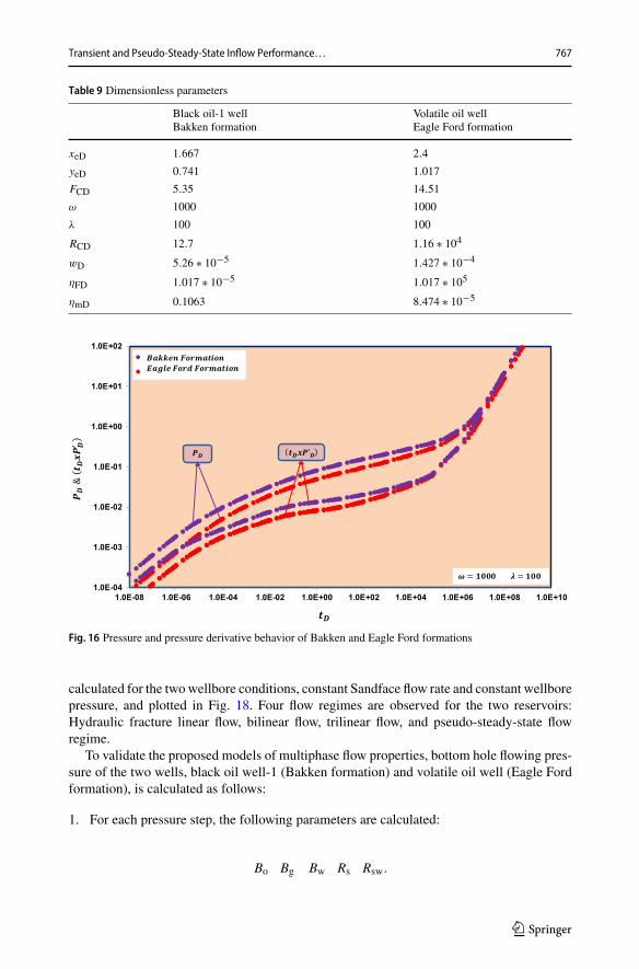
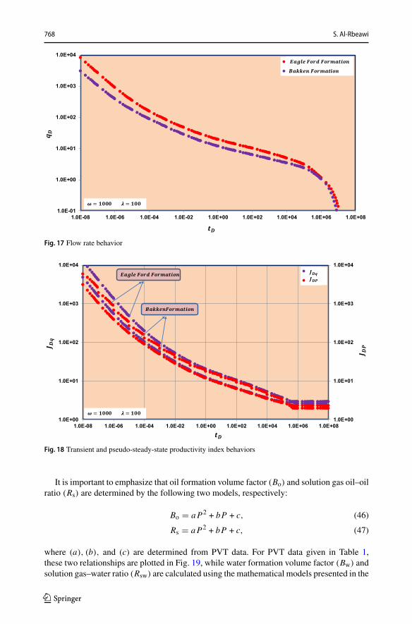
Dimensionless pressure and pressure derivative of Bakken and Eagle Ford formations arecalculated using dimensionless parameters given in Table 9 and plotted as shown in Fig. 16,while dimensionless flow rate behavior is calculated and plotted as shown in Fig. 17. Transientand pseudo-steady-state productivity index of the two reservoirs in dimensionless form is

123

Transient and Pseudo-Steady-State Inflow Performance… 767

Table 9 Dimensionless parameters

Black oil-1 wellBakken formation

Volatile oil wellEagle Ford formation

xeD 1.667 2.4

yeD 0.741 1.017

FCD 5.35 14.51

ω 1000 1000

λ 100 100

RCD 12.7 1.16 ∗ 104

wD 5.26 ∗ 10−5 1.427 ∗ 10−4

ηFD 1.017 ∗ 10−5 1.017 ∗ 105

ηmD 0.1063 8.474 ∗ 10−5

1.0E-04

1.0E-03

1.0E-02

1.0E-01

1.0E+00

1.0E+01

1.0E+02

1.0E-08 1.0E-06 1.0E-04 1.0E-02 1.0E+00 1.0E+02 1.0E+04 1.0E+06 1.0E+08 1.0E+10

Series3

Series4

Fig. 16 Pressure and pressure derivative behavior of Bakken and Eagle Ford formations

calculated for the twowellbore conditions, constant Sandface flow rate and constant wellborepressure, and plotted in Fig. 18. Four flow regimes are observed for the two reservoirs:Hydraulic fracture linear flow, bilinear flow, trilinear flow, and pseudo-steady-state flowregime.

To validate the proposed models of multiphase flow properties, bottom hole flowing pres-sure of the two wells, black oil well-1 (Bakken formation) and volatile oil well (Eagle Fordformation), is calculated as follows:

1. For each pressure step, the following parameters are calculated:

Bo Bg Bw Rs Rsw.

123

768 S. Al-Rbeawi

1.0E-01

1.0E+00

1.0E+01

1.0E+02

1.0E+03

1.0E+04

1.0E-08 1.0E-06 1.0E-04 1.0E-02 1.0E+00 1.0E+02 1.0E+04 1.0E+06 1.0E+08

Series1

Fig. 17 Flow rate behavior

1.0E+00

1.0E+01

1.0E+02

1.0E+03

1.0E+04

1.0E+00

1.0E+01

1.0E+02

1.0E+03

1.0E+04

1.0E-08 1.0E-06 1.0E-04 1.0E-02 1.0E+00 1.0E+02 1.0E+04 1.0E+06 1.0E+08

Series3

Series1

Fig. 18 Transient and pseudo-steady-state productivity index behaviors

It is important to emphasize that oil formation volume factor (Bo) and solution gas oil–oilratio (Rs) are determined by the following two models, respectively:

Bo � aP2 + bP + c, (46)

Rs � aP2 + bP + c, (47)

where (a), (b), and (c) are determined from PVT data. For PVT data given in Table 1,these two relationships are plotted in Fig. 19, while water formation volume factor (Bw) andsolution gas–water ratio (Rsw) are calculated using the mathematical models presented in the

123

Transient and Pseudo-Steady-State Inflow Performance… 769

Bo = 1E-08P2 + 5E-05P + 1.0497R² = 1

Rs = 2E-05P2 + 0.1333P + 27.227R² = 0.9999

0

200

400

600

800

1000

1200

1400

1600

1

1.1

1.2

1.3

1.4

1.5

1.6

1.7

1.8

1.9

0 1000 2000 3000 4000 5000 6000

Series1

Series2

Fig. 19 Oil formation volume factor and solution gas–oil ratio

Bw = -7E-09P2 - 4E-06P + 1.039R² = 1

Rsw = -9E-08P2 + 0.0022P+ 0.7883R² = 1

0

2

4

6

8

10

12

0.60

0.65

0.70

0.75

0.80

0.85

0.90

0.95

1.00

1.05

1.10

0 1000 2000 3000 4000 5000 6000

Fig. 20 Water formation volume factor and solution gas–water ratio

literature, Eqs. (9) and (10), and plotted in Fig. 20. Similarly, gas formation volume factor iscalculated and plotted in Fig. 21.

2. Calculate total flow rate (qt ) using Eq. (22) and total formation volume factor (Bt) usingEq. (23).

3. Calculate multiphase reservoir total compressibility (ct)mp using Eq. (45).4. Calculate multiphase reservoir total mobility using Eq. (44).5. Calculate wellbore pressure drop (�Pwf) by:

123

770 S. Al-Rbeawi

Bg = 2.9481x-0.997

R² = 0.9937

0.000

0.005

0.010

0.015

0.020

0 1000 2000 3000 4000 5000 6000

Fig. 21 Gas formation volume factor

Fig. 22 Comparison for bottom hole flowing pressure; a Bakken formation and b Eagle Ford formation

�Pwf � 141.2(qtBt)PwD

km(kμ

)

mp

, (48)

where (PwD) is dimensionless wellbore pressure drop calculated by Eq. (16) for differentdimensionless production times.

6. Real production time is calculated from dimensionless production time by:

t � ∅(ct)mpx2f tD

0.0002637km(kμ

)

mp

. (49)

The calculated bottom hole flowing pressure is plotted and compared with the pressurerecords of the two reservoirs. Excellent matching is obtained as shown in Fig. 22.

123

Transient and Pseudo-Steady-State Inflow Performance… 771

0

1000

2000

3000

4000

5000

6000

0 200 400 600 800 1000 1200 1400 1600 1800 2000

Fig. 23 The IPR for different flow regimes—Bakken formation

0500

1000150020002500300035004000450050005500600065007000750080008500

0 500 1000 1500 2000 2500 3000

Fig. 24 The IPR for different flow regimes—Eagle Ford formation

The IPRs of Bakken and Eagle Ford reservoirs assuming constant Sandface flow rate fordifferent flow regimes are plotted in Figs. 23 and 24, respectively. The starting time of eachflow regime is determined using Eq. (49). The following points are inferred from these twoplots:

1. The productivity of Eagle Ford formation for the same pressure drop is better than ofBakken formation.

2. It takes longer time in Eagle Ford formation to reach pseudo-steady-state flow comparedwith Bakken formation because Eagle Ford formation has ultralow matrix permeability

123

772 S. Al-Rbeawi

(km � 0.5 ∗ 10−6 md

)less than the one in Bakken formation

(km � 6.27 ∗ 10−4 md

).

Similar thing is observed for all flow regimes.3. Trilinear flow regime dominates fluid flow in Eagle Ford formation longer than in Bakken

formation as the fracture half-length is shorter than the fracture half-length of Bakkenformation.

5 Conclusions

1. Multiphase flow may have significant impact on pressure heavier, decline rate pattern,and productivity index as well as inflow performance relationship of reservoirs regardlessthe inner boundary condition of the wellbore whether it is constant Sandface flow rate orconstant wellbore pressure.

2. Multiphase reservoir total mobility and compressibility significantly change with reser-voir pressure. Reservoir compressibility demonstrates more changes than the mobilityespecially at low reservoir pressure; however, it shows more steady-state changes at highreservoir pressure compared with the mobility.

3. Multiphase reservoir total mobility and compressibility show similar behavior for dif-ferent reservoirs and different reservoir fluids. Therefore, very slight differences in themathematical models of these two parameters are seen for different PVT data sets.

4. Multiphase flow may not have significant impact on the inflow performance relationshipat late production time when pseudo-steady-sate or boundary-dominated flow regime isthe dominant flow pattern.

5. There is no significant difference between the constant Sandface flow rate and constantwellbore pressure conditions; however, the inflow performance relationship of constantSandface flow rate is better than of constant wellbore pressure.

Appendix

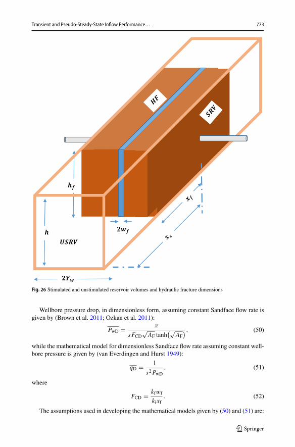
Consider the formation shown in Fig. 25 where multiple hydraulic fractures propagate in thestimulated reservoir volume (SRV). The formation could have also unstimulated part (USRV)where the stimulation process does not have any impact on the porous media. Formationboundaries are indicated by (2xe, 2ye) and fracture half-length is (xf). Hydraulic fracturesconsidered fully penetrate the formation, i.e., hydraulic fracture height is considered equalto the formation thickness. Stimulated and unstimulated reservoir volumes and hydraulicfracture dimensions are depicted in Fig. 26.

Fig. 25 Schematic drawing for a hydraulically fractured reservoir

123

Transient and Pseudo-Steady-State Inflow Performance… 773

Fig. 26 Stimulated and unstimulated reservoir volumes and hydraulic fracture dimensions

Wellbore pressure drop, in dimensionless form, assuming constant Sandface flow rate isgiven by (Brown et al. 2011; Ozkan et al. 2011):

PwD � π

sFCD√AF tanh

(√AF

) , (50)

while the mathematical model for dimensionless Sandface flow rate assuming constant well-bore pressure is given by (van Everdingen and Hurst 1949):

qD � 1

s2PwD, (51)

where

FCD � kfwf

kixf. (52)

The assumptions used in developing the mathematical models given by (50) and (51) are:

123

774 S. Al-Rbeawi

1. Constant porosity and uniform reservoir thickness.2. Symmetrically distributed hydraulic fractureswith symmetrical hydraulic fracture dimen-

sions.3. Fractures fully penetrate the formation in the vertical direction.

Initial reservoir conditions are:

PD(xD, yD, tD � 0.0) � PDi, (53)

while reservoir inner and outer boundary conditions are:

∂PD∂xD

∣∣∣∣xD�xeD

� 0.0, (54)

∂PwD∂xD

∣∣∣∣xD�0.0

� π

sFCD. (55)

The parameter (AF) refers to the configurations of the stimulated and unstimulated reser-voir volumes in addition to the petrophysical properties of the two volumes. Mathematically,this parameter is written:

AF � 2BF

FCD+

s

ηfD, (56)

where

BF � √Ar tanh

[√Ar(yeD − wD/2)

], (57)

Ar � Br

RCDyeD+ s f (s), (58)

Br �√

s

ηmDtanh

[√s

ηmD(xeD − 1)

], (59)

RCD � ki xfkmye

, (60)

ηmD � ηm

ηi, (61)

ηfD � ηf

ηi, (62)

xeD � xexf

, (63)

yeD � yexf

, (64)

wD � wf

xf, (65)

PD �ki

(kμ

)

mph�P

141.2(qtBt), (66)

tD �0.000263ki

(kμ

)

mpt

(∅ct)fx2f. (67)

123

Transient and Pseudo-Steady-State Inflow Performance… 775

References

Agarwal, R.G., Carter, R.D., Pollock, C.B.: Evaluation and performance prediction of low-permeability gaswells stimulated by massive hydraulic fracturing. JPT 31(03), 362–372 (1979). https://doi.org/10.2118/6838-pa

Al-Khalifa, A.J., Horne, R.N., Aziz, K.: Multiphase well test analysis: pressure and pressure-squared methods.Paper presented at the SPE California regional meeting held in Bakersfield, CA, USA, April 5–7 (1989).https://doi.org/10.2118/18803-ms

Aulisa, E., Ibragimov, A., Walton, J.: A new method for evaluating the productivity index of nonlinear flows.SPE J. 14(04), 693–706 (2009). https://doi.org/10.2118/108984-pa

Ayan,C., Lee,W.J.:Multiphase pressure buildup analysis: field examples. Paper presented at theSPECaliforniaregional meeting held in Long Beach, California, USA, March 23–25 (1988). https://doi.org/10.2118/17412-ms

Bello, R.O.: Rate transit analysis in shale gas reservoirs with transient linear behavior. PhD, Texas A&MUniversity, Collage Station, TX, USA (2008)

Behmanesh, H., Mattar, L., Thompson, J.M., Anderson, D.M., Nakaska, D.W., Clarkson, C.R.: Treatment ofrate-transient analysis during boundary-dominated flow. SPEJ (2018). https://doi.org/10.2118/189967-pa

Behmanesh, H., Clarkson, C.R., Tabatabaie, S.H., Heidari Sureshjani, M.: Impact of distance-of-investigationcalculations on rate-transient analysis of unconventional gas and light-oil reservoirs: new formulationsfor linear flow. JCPT 54(06), 509–519 (2015). https://doi.org/10.2118/178928-pa

Bennett, C.O., Reynolds, A.C., Raghavan, R., Elbel, J.L.: Performance of finite-conductivity, vertically frac-tured wells in single-layer reservoirs. SPE Form. Eval. 1(04), 399–412 (1986). https://doi.org/10.2118/11029-pa

Boe,A., Skjaeveland, S.M.,Whitson,C.H.: Two-phase pressure test analysis. SPEForm.Eval.04(04), 601–610(1989). https://doi.org/10.2118/10224-pa

Brown, M., Ozkan, E., Raghavan, R., Kazemi, H.: practical solutions for pressure-transient responses offractured horizontal wells in unconventional shale reservoirs. SPE Reserv. Eval. Eng. 14(6), 663–676(2011). https://doi.org/10.2118/125043-pa

Camacho, R.G., Raghavan, R.: Inflow performance relationships for solution-gas-drive reservoirs. JPT 41(05),541–550 (1989). https://doi.org/10.2118/16204-pa

Camacho, R.G., Raghavan, R., Reynolds, A.C.: Response of wells producing layered reservoirs: unequalfracture length. SPE Form. Eval. 2(01), 9–28 (1987). https://doi.org/10.2118/12844-pa

CamachoVelazquez, R., Fuentes-Cruz,G., Vasquez-Cruz,M.A.:Decline-curve analysis of fractured reservoirswith fractal geometry. SPE Reserv. Eval. Eng. 11(03), 606–619 (2008). https://doi.org/10.2118/104009-pa

Cinco-Ley, H.: Unsteady-state pressure distribution created by a slantedwell or awell with an inclined fracture.PhD dissertation, Stanford University, California, USA (1974)

Cinco-Ley, H., Samaniego, F.: Transient pressure analysis for fractured wells. JPT 33(09), 1749–1766 (1981).https://doi.org/10.2118/7490-pa

Cinco-Ley,H., Ramey,H.J.,Miller, F.G.:Unsteady-state pressure distribution created by awellwith an inclinedfracture. Paper presented at the 50th annual fall meeting of the society of petroleum engineers of AIMEheld in Dallas, TX, USA (1975). https://doi.org/10.2118/5591-ms

Cinco, L., Samaniego, V., Dominguez, A.: Transient pressure behavior for a well with a finite-conductivityvertical fracture. SPEJ 18(04), 253–264 (1978). https://doi.org/10.2118/6014-pa

Cipolla, C.L.: Modeling production and evaluating fracture performance in unconventional gas reservoirs. JPT61(09), 84–90 (2009). https://doi.org/10.2118/118536-jpt

Chen, A., Jones, J.R.: Use of pressure/rate deconvolution to estimate connected reservoir-drainage volumein naturally fractured unconventional-gas reservoirs from canadian rockies foothills. SPE Reserv. Eval.Eng. 15(03), 290–299 (2012). https://doi.org/10.2118/143016-pa

Chu,W.-C., Reynolds, A.C., Raghavan, R.: Pressure transient analysis of two-phase flow problems. SPE Form.Eval. 01(02), 151–164 (1986). https://doi.org/10.2118/10223-pa

Duong, A.N.: Rate-decline analysis for fracture-dominated shale reservoirs. SPE Reserv. Eval. Eng. 14(03),377–387 (2011). https://doi.org/10.2118/137748-pa

El-Banbi, A.H.: Analysis of tight gas wells. PhD, Texas A&M University, Collage Station, TX, USA (1998)Fetkovich, M.J.: The isochronal testing of oil wells. Paper presented at the 48th Annual fall meeting of the

SPE of AIME in Las Vegas, Nevada, USA, 30 Oct–3 Nov (1973). https://doi.org/10.2118/4529-msFraim, M.L., Wattenbarger, R.A.: Decline curve analysis for multiphase flow. Paper presented at the SPE 63rd

annual technical conference & exhibition held in Houston, TX, USA, October 2–5 (1988). https://doi.org/10.2118/18274-ms

123

776 S. Al-Rbeawi

Fuentes-Cruz, G., Valko, P.P.: Revisiting the dual-porosity/dual-permeability modeling of unconventionalreservoirs: the induced-interporosity flow field. SPE J. 20(01), 125–141 (2015). https://doi.org/10.2118/173895-pa

Fuentes-Cruz, G., Gildin, E., Valko, P.P.: Analyzing production data from hydraulically fractured wells: theconcept of induced permeability field. SPE Reserv. Eval. Eng. 17(02), 220–232 (2014). https://doi.org/10.2118/163843-pa

Gallice, F., Wiggins, M.L.: A comparison of two-phase inflow performance relationships. SPE Prod. Facil.19(02), 100–104 (2004). https://doi.org/10.2118/88445-pa

Gringarten, A.C., Ramey, H.J.: The use of source and green’s function in solving unsteady-flow problems inreservoirs. SPEJ 13(05), 286–296 (1973). https://doi.org/10.2118/3818-pa

Gringarten, A.C., Ramey, H.J., Raghavan, R.: Unsteady-state pressure distributions created by a well witha single infinite-conductivity vertical fracture. SPEJ 14(04), 347–360 (1974). https://doi.org/10.2118/4051-pa

Golan, M., Whitson, C.H.: Well Performance, 2nd edn. Prentice-Hall Inc (1995). Printed in Norway by Tapir(1996)

Guppy, K.H., Kumar, S., Kagawan, V.D.: Pressure-transient analysis for fractured wells producing at constantpressure. SPE Form. Eval. 3(01), 169–178 (1988). https://doi.org/10.2118/13629-pa

Hagoort, J.: Automatic decline-curve analysis ofwells in gas reservoirs. SPEReserv. Eval. Eng. 6(06), 433–440(2003). https://doi.org/10.2118/77187-pa

Holditch, S.A., Morse, R.A.: The effects of non-Darcy flow on the behavior of hydraulically fractured gaswells (includes associated paper 6417). JPT 28(10), 1169–1179 (1976). https://doi.org/10.2118/5586-pa

Kamal, M.M., Pan, Y.: Use of transient data to calculate absolute permeability and average fluid saturations.SPE Reserv. Eval. Eng. 13(02), 306–312 (2010). https://doi.org/10.2118/113903-pa

Kamal, M.M., Pan, Y.: Pressure transient testing under multiphase flow conditions. Paper presented at the SPEMiddle East Oil and gas show and conference held in Manama, Bahrain, Sep. 25–28 (2011). https://doi.org/10.2118/113903-pa

Kanfar, M.S., Clarkson, C.R.: Rate dependence of bilinear flow in unconventional gas reservoirs. SPE Reserv.Eval. Eng. 5, 7 (2018). https://doi.org/10.2118/186092-pa

Kuchuk, F.J.: Applications of convolution and deconvolution to transient well tests. SPE Form. Eval. 5(04),375–384 (1990). https://doi.org/10.2118/16394-pa

Ibrahim, M., Wattenbarger, R.A.: Rate dependence of transient linear flow in tight gas wells. JCPT 45(10),18–20 (2006). https://doi.org/10.2118/06-10-tn2

Ilk, D., Valko, P.P., Blasingame, T.A.: Deconvolution of variable-rate reservoir performance data using B-splines. SPE Reserv. Eval. Eng. 9(05), 582–595 (2006). https://doi.org/10.2118/95571-pa

Izadi,M., Yildiz, T.: Transient flow in discretely fractured porousmedia. SPEJ 14(02), 362–373 (2009). https://doi.org/10.2118/108190-pa

Larsen, L., Hegre, T.M.: Pressure transient analysis of multifractured horizontal wells. Paper (SPE-28389)presented at the SPE Annual technical conference & exhibition held in New Orleans, Louisiana, USA,25–28 September (1994).https://doi.org/10.2118/28389-ms

Lee, J., Wattenbarger, R.A.: Gas Reservoir Engineering. SPE Textbook Series, vol. 5. Society of PetroleumEngineers, Houston (1996)

Levitan, M.M.: Practical application of pressure-rate deconvolution to analysis of real well tests. SPE Reserv.Eval. Eng. 8(02), 113–121 (2005). https://doi.org/10.2118/84290-pa

Li, X., Liang, J., Xu, W., Li, X., Tan, X.: The new method on gas-water two phase steady state productivity offractured horizontal well in tight gas reservoir. Geo Energy Res. 1(02), 105–111 (2017). https://doi.org/10.26804/ager.2017.02.06

Luo, H., Mahiya, G., Pannett, S., Benham, P.H.: The use of rate-transient-analysis modeling to quantifyuncertainties in commingled tight gas production-forecasting and decline-analysis parameters in theAlberta deep basin. SPE Reserv. Eval. Eng. 17(02), 209–219 (2014). https://doi.org/10.2118/147529-pa

Martin, J.C.: Simplified equations of flow in gas drive reservoirs and the theoretical foundation of multiphasepressure buildup analyses. SPE Gen. 261(01), 321–323 (1959)

Martin, J.C., James, D.M.: Analysis of pressure transients in two-phase radial flow. SPE J. 3(02), 116–126(1963). https://doi.org/10.2118/425-pa

Muskat, M.: The flow of homogenous fluids through porous media. McGraw Hill Book Co., Inc., New York(1937)

Muskat, M., Meres, M.W.: The flow of heterogeneous fluids in porous media. J. Appl. Phys. 7(09), 346–363(1936). https://doi.org/10.1063/1.1745403

Nobakht, M., Clarkson, C.R., Kaviani, D.: New and improved methods for performing rate-transient analysisof shale gas reservoirs. SPE Reserv. Eval. Eng. 15(03), 335–350 (2012). https://doi.org/10.2118/147869-pa

123

Transient and Pseudo-Steady-State Inflow Performance… 777

Ozkan, E.: Performance of horizontal wells. PhD dissertation, The University of Tulsa, OK, USA (1988)Ozkan, E., Raghavan, R.: New solutions for well-test-analysis problems: part 1 analytical considerations. SPE

Form. Eval. 6(03), 359–368 (1991a). https://doi.org/10.2118/18616-paOzkan, E., Raghavan, R.: New solutions for well-test-analysis problems: part 2 computational considerations

and applications. SPE Form. Eval. 6(03), 369–378 (1991b). https://doi.org/10.2118/18616-paOzkan, E., Brown, M.L., Raghavan, R., Kazemi, H.: Comparison of fractured-horizontal-well performance in

tight sand and shale reservoirs. SPE Reserv. Eng. Eval. 14(02), 248–256 (2011). https://doi.org/10.2118/121290-pa

Perrine, R. L.: Analysis of pressure-buildup curves. Drilling and production practice, API-56-482, New York,USA (1956)

Prats, M., Levine, J.S.: Effect of vertical fractures on reservoir behavior- results on oil and gas flow. JPT15(10), 1119–1126 (1963). https://doi.org/10.2118/593-pa

Raghavan, R.: Well test analysis: wells producing by solution gas drive. SPEJ 16(04), 196–208 (1976). https://doi.org/10.2118/5588-pa

Raghavan, R.: Well-test analysis for multiphase flow. SPE Form. Eval. 4(04), 585–594 (1989). https://doi.org/10.2118/14098-pa

Raghavan, R., Uraiet, A., Thomas, G.W.: Vertical fracture height: effect on transient flow behavior. SPEJ18(04), 265–277 (1978). https://doi.org/10.2118/6016-pa

Raghavan, R.S., Chen, C.-C., Agarwal, B.: An analysis of horizontal wells intercepted by multiple fractures.SPEJ 2(03), 235–245 (1997). https://doi.org/10.2118/27652-pa

Shahamat, M.S., Mattar, L., Aguilera, R.: Analysis of decline curves on the basis of beta-derivative. SPEReserv. Eval. Eng. 18(02), 214–227 (2015). https://doi.org/10.2118/169570-pa

Soliman, M.Y., Hunt, J.L., El Rabaa, A.M.: Fracturing aspects of horizontal wells. JPT 42(08), 966–973(1990). https://doi.org/10.2118/18542-pa

Standing, M.B.: Concerning the calculation of inflow performance of wells producing from solution gas drivereservoirs. JPT 23(09), 1141–1142 (1971). https://doi.org/10.2118/3332-pa

Stone, H.L.: Probability model for estimating three-phase relative permeability. JPT 22(2), 214–218 (1970).https://doi.org/10.2118/2116-pa

Stone, H.L.: Estimation of three-phase relative permeability and residual oil data. JCPT 12(4), 53–61 (1973).https://doi.org/10.2118/73-04-06

Tabatabaie, S.H., Pooladi-Darvish, M.: Multiphase linear flow in tight oil reservoirs. SPE Reserv. Eval. Eng.20(01), 184–196 (2017). https://doi.org/10.2118/180932-pa

Torcuk, M.A., Kurtoglu, B., Alharthy, N., Kazemi, H.: Analytical solutions for multiple matrix in fracturedreservoirs: application to conventional and unconventional reservoirs. SPEJ 18(05), 969–981 (2013).https://doi.org/10.2118/164528-pa

Uzun, I., Kurtoglu, B., Kazemi, H.: Multiphase rate-transient analysis in unconventional reservoirs: theoryand application. Paper presented at the SPE/CSUR unconventional resources conference held in Calgary,Alberta, Canada, September 30–October 2 (2014).https://doi.org/10.2118/171657-pa

Uzun, I., Kurtoglu, B., Kazemi, H.: Multiphase rate-transient analysis in unconventional reservoirs: theoryand application. SPE Reserv. Eval. Eng. 19(04), 553–566 (2016). https://doi.org/10.2118/171657-pa

Van Everdingen, A.F., Hurst, W.: The application of the Laplace transformation to flow problems in reservoirs.Pet. Trans. AIME 186, 305–324 (1949). https://doi.org/10.2118/949305-g

Vogel, J.V.: Inflow performance relationships for solution-gas drive wells. JPT 20(01), 83–92 (1968). https://doi.org/10.2118/1476-pa

Wan, J., Aziz, K.: Multiple hydraulic fractures in horizontal wells. Paper (SPE-54627) presented at the SPEWestern regional meeting held in Anchorage, Alaska, USA, 26–27 May (1999). https://doi.org/10.2118/54627-ms

Wiggins, M.L.: Generalized inflow performance relationships for three-phase flow. SPE Reserv. Eng. 9(03),181–182 (1994). https://doi.org/10.2118/25458-pa

123