Scholars' Mine Scholars' Mine

Masters Theses Student Theses and Dissertations

1970

Transient response of a vibration isolation system Transient response of a vibration isolation system

Hemendra Shantilal Acharya

Follow this and additional works at: https://scholarsmine.mst.edu/masters_theses

Part of the Mechanical Engineering Commons

Department: Department:

Recommended Citation Recommended Citation Acharya, Hemendra Shantilal, "Transient response of a vibration isolation system" (1970). Masters Theses. 7174. https://scholarsmine.mst.edu/masters_theses/7174

This thesis is brought to you by Scholars' Mine, a service of the Missouri S&T Library and Learning Resources. This work is protected by U. S. Copyright Law. Unauthorized use including reproduction for redistribution requires the permission of the copyright holder. For more information, please contact scholarsmine@mst.edu.

TRANSIENT RESPONSE OF A

VIBRATION ISOLATION SYSTEM

BY

HEMENDRA SHANTILAL ACHARYA, 1943-

A

THESIS

submitted to the faculty of

UNIVERSITY OF MISSOURI - ROLLA

in partial fulfillment of the requirements for the

Degree of

MASTER OF SCIENCE IN MECHANICAL ENGINEERING

Rolla, ~1issouri

1970

Approved by

T2499 c.l 74 pages

ABSTRACT

A practical procedure for investigating the performance of a

vibration isolation system under transient conditions is presented.

For this investigation, an induction motor with an unbalanced rotor

is studied during the period when it accelerates to its operating

speed from rest.

ii

Using Newton's second law of motion, equations of motion are

derived, first neglecting and then considering the effect of "inertia

torque". This torque is produced by the inertia force resulting from

vertical acceleration of the unbalanced mass. The equations are

solved on a digital computer using the Runge-Kutta method of order 4.

The results obtained are compared with those obtained using Simpson's

and Runge-Kutta methods of order 4 of the Continuous System Modeling

Program. For the case when there is no external load, an attempt was

made to obtain the responses of the system by the Convolution Integral

Solution of the K. A. Foss method.

A study of steady state and transient analyses for "inertia" and

"no inertia" cases is carried out. From the results obtained, graphs

are plotted and guidelines useful for design of vibration isolators

are given.

ACKNOWLEDGEMENTS

The author wishes to express his appreciation to Dr. William S.

Gatley for the suggestion of the topic of this thesis and for his

encouragement, direction and assistance throughout the course of

this thesis.

The author is thankful to Elizabeth Wilkins for her cooperation

in typing this thesis.

iii

iv

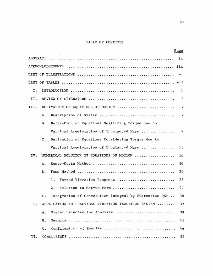
TABLE OF CONTENTS

ABSTRACT ......................................................... ii

ACKNOWLEDGEMENTS . . . • . . . • . • . • . • . • . . . . . • . • . • . . . • . . . . . . . . • . . . . . . . . . . iii

LIST OF ILLUSTRATIONS . • . . . . . . . . . . • . • . • . • . . . • . • . • . . . • . . . . . . . . . . . . . vi

LIST OF TABLES .......••••.••......•...•..•.••.•.•.•.......••..•.. vii

I. INTRODUCTION . • . • . . • • . . . . . . . • • . . . • . • • • • . • . • • • . • • . . . . • • . . . . . . 1

II. REVIEW OF LITERATURE . . • . • • . • . . . . • • • • . . • . . . • . • . . . • . • . . . . . . . . 3

III. DERIVATION OF EQUATIONS OF MOTION.......................... 7

A. Description of System • • . . . . . . . • • . . . . . . . . . . . . . . • . • . . . . • . 7

~. Derivation of Equations Neglecting Torque due to

Vertical Acceleration of Unbalanced Mass ....••......... 9

C. Derivation of Equations Considering Torque due to

Vertical Acceleration of Unbalanced Mass .....•......... 13

IV. NUMERICAL SOLUTION OF EQUATIONS OF MOTION .......•...•.•.... 16

A. Runge-Kutta Method . . . . . . . . . . . . • . . . • • . . . . . . . . . . • . . . . . . . . 16

B. Foss Method 20

1. Forced Vibration Response . . . . . . . . . . • . . . . . . . . . • . . . . . 25

2. Solution in Matrix Form ......................•..... 27

C. Integration of Convolution Integral by Subroutine QSF .. 38

V. APPLICATION TO PRACTICAL VIBRATION ISOLATION SYSTEM .....•.. 39

A. System Selected for Analysis ...........•............... 39

B. Results . . . . . • . . . . . . . . . . . • . . . . . • . . . . . . . . . . . . . • . . . . . . . . . . 41

C. Confirmation of Results . . • . . . • . . . . . . . . . . . . . . . . . . . . . . . . . 44

VI. CONCLUSIONS . • . . . . . . . • • . . . . . . . . . . . • • . . • . . . . . . . . . . . . . . . . . . . . . 52

VII. PiJ!PENDICES ...•••.•••.••...•..••••.....•...•••••.•...•.•••••

A. Calculation of Natural Frequencies of Undamped System ..

v

Page

54

55

B. Derivation of Equation for Accelerating Torque .•••.•..• 57

C. Calculation of the Moment of Inertia of the Rotor •••... 64

VIII. BIBLIOG'RA.PHY . . . . • • . . . • . • . • . • . • . • . • . • • . . . . • . . • • . . . . • . . . . . . • . 65

IX. VITA • • • • • • • • • • • • • • • • • • • • • • • • • • . • • • • • • • • • • • • • • • • • • • • • • • • • • • • 6 7

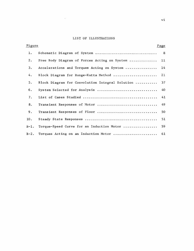
Figure

1.

2.

3.

4.

5.

6.

7.

8.

9.

10.

B-1.

B-2.

LIST OF ILLUSTRATIONS

Schematic Diagram of System

Free Body Diagram of Forces Acting on System ............. .

Accelerations and Torques Acting on System ............... .

Block Diagram for Runge-Kutta Method ................•.....

Block Diagram for Convolution Integral Solution .......... .

System Selected for Analysis ............................. .

List of Cases Studied ...•................•................

Transient Responses of Motor

Transient Responses of Floor

Steady State Responses

Torque-Speed Curve for an Induction Motor ................ .

Torques Acting on an Induction Motor ..................... .

vi

8

11

14

21

37

40

41

49

50

51

59

61

vii

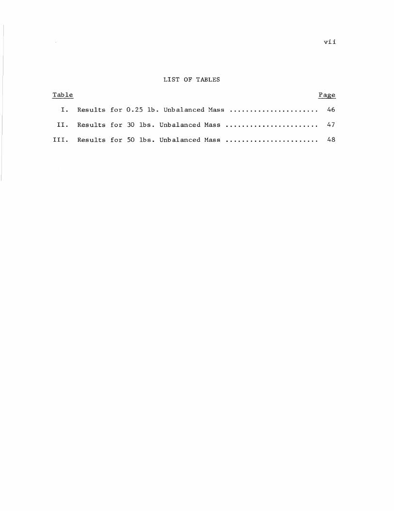
LIST OF TABLES

Table Page

I. Results for 0.25 lb. Unbalanced Mass ...................... 46

II. Results for 30 lbs. Unbalanced Mass ....................... 47

III. Results for 50 lbs. Unbalanced Hass ....................... 48

I. INTRODUCTION

In this thesis, a practical procedure is developed for vibration

isolation analysis during the transient period.

Generally, most machines and structures experience vibration for

two reasons: (1) due to changes in the relative positions of the

1

elements and (2) due to forces generated within the structures involved.

Our discussion is restricted to the latter case.

Shaking forces produced during the operation of machinery can be

categorized as follows:

1. Forces due to the inertia of unbalanced rotating and reciprocating

members.

2. Forces due to operation of the machinery itself.

All of these forces may be transmitted to the structure upon

which the machine is mounted. The supporting structure thus experi­

ences vibration that depends upon the nature of the forces and on the

characteristics of the structure. These vibrations may affect the

operation of other machinery mounted on the same structure, or in some

instances, may cause structural failures due to cyclic fatigue.

To avoid such harmful effects, it becomes necessary to eliminate

or isolate the forces producing the unwanted vibration. This can be

achieved in two ways: (1) by dynamic balancing of the forces which

cause the vibration and (2) by isolating the support from such forces.

It has been found that dynamic balancing of forces is not practical in

many cases. In its simplest form, isolating a machine or particular

component means mounting the machine or component upon properly

designed isolators, so that forces transmitted to the supporting

structure are minimized.

Often the vibration is caused by an oscillatory force which

exists at a constant frequency. This condition is designated "steady

state", because an identical pattern of vibration amplitude is re-

2

peated during each cycle. Sometimes, however, one observes a different

pattern of vibration which is not periodic. This condition is usually

designated "transient" and is produced by a suddenly applied force or

by a force which changes with time.

In the steady state case when the exciting force is harmonic,

the steady state vibration takes place at the frequency of the excita­

tion. During the "transient" period, additional vibrations at one or

more of the resonant frequencies may be superimposed upon the vibration

at the excitation frequency. If the forcing frequency varies with time,

dangerously large amplitudes may result when the excitation frequency

approaches one of the resonant frequencies of the system.

To investigate the performance of vibration isolation systems

during the transient period, a system in which an electric motor is

mounted on isolators is studied. The supporting structure (floor) is

represented by a mass and spring combination and the isolator is

represented by a linear spring in parallel with a viscous damper.

Excitation of the system is caused by unbalanced rotating masses

within the motor rotor or the machinery driven by the motor.

In the following sections, the equations of motion for the system

are derived and solved by first neglecting and then considering the

effect of inertia torque produced by the vertical acceleration of

unbalanced mass.

II. REVIEW OF LITERATURE

Vibration isolation of machinery is treated to some extent in

almost every text or reference dealing with vibration analysis. In

addition, numerous technical papers on the general subject of vibra-

tion isolation have been published in recent years.

* S. Timoshenko and D. H. Young [1] describe the theory of free

and forced vibrations of conservative systems, giving special atten-

tion to the theory of vibration isolation.

Paul A. Crafton [7] has discussed the isolation of a machine

from steady state sinusoidal components of motion. The machine has

an independent force acting on it and the foundation has a motion

that is independent of the force input. Crafton has assumed that

the force and motion input functions are sinusoidal with time. He

3

has also described a feedback system for isolation from discontinuous

inputs. He has achieved isolation as far as the steady state

component of motion of the machine is concerned, for cases of with

and without damping.

R. T. Lowe [8] has discussed control of vibration through

isolation of forces or motions. He has discussed only undamped

vibration. For this, he uses a graph of the fraction of force and

displacement transmitted by the system (i.e., transmissibility) versus

the ratio of the forcing frequency to the undamped natural frequency

to select a particular frequency ratio for which the value of trans-

missibility is less than unity. This frequency ratio is used to

* Numbers in brackets refer to list of references at end of thesis.

determine the system parameters.

R. Plunkett [9], by citing examples of a turbine rotor and an

automatic washing machine, has analyzed steady state vibration. He

defines the steady state dynamic characteristics of a given system

in terms of mechanical impedence, which is the ratio of an applied

sinusoidal force to the resulting vibration velocity. The term

mobility is defined as the inverse of mechanical impedence. By

simple analysis, Plunkett derives the transmissibility ratio in

terms of mobility and shows that to have effective isolation, the

isolator should have high mobility compared to the mobilities of

4

the machine and foundation. He has discussed steady state isolation

with viscous damping.

J. C. Snowdon [10] presents an analysis of natural or synthetic

rubbers used as damped resilient springs between an absorber mass and

the principal mass. He has studied the steady state case with viscous

damping.

G. J. Andrews' paper [11] is mainly concerned with the rigid­

body-on-resilient-mounts problem. The author has derived the

equations of motion for a rigid body of arbitrary shape, supported

at three or more noncolinear points by resilient mounts which have

damping. His solution (for the steady state case) is given in

programs suitable for solution by a high speed digital computer.

J. E. Ruzica and R. D. Cavanaugh [12] have described an elas­

tically supported damper system, which eliminates the damping force

at high frequencies. They have plotted absolute and relative trans­

missibility values for zero and infinite damping. Optimum damping

is determined by differentiating the transmissibility equation with

respect to frequency ratio and equating the result to zero.

Hanley's paper [13] explains the dynamics underlying displace­

ment-excited motions and provides curves whereby the dynamic forces

can be calculated.

Carter and Liu [14] have analyzed a dynamic vibration absorber

for the case where both the main and absorber springs have nonline­

arities. A one term approximation solution is assumed for the

motion of the two masses and the resulting amplitude equation is

solved using a graphical procedure.

5

K. A. Foss [15] has developed a method for solving non-classically

damped multi-degree of freedom systems. He transforms the original

system into 2N space in order to uncouple the equations of motion (see

chapter IVB). The solution is in matrix form.

B. B. Patel [16] has developed computer programs for solving

vibration problems by the Foss method. These programs give eigenvalues,

eigenvectors and the transient response of the system. Patel has

also obtained the complete response of the system subjected to a

sinusoidal force. His programs can be used for any system provided

the Convolution Integral is evaluated by hand. In this thesis, the

complex Convolution Integral solution is obtained as computer

output, after the integral has been separated into real and imaginary

parts.

It was found from the literature surveyed that relatively little

research has been published concerning the transient response of

vibration isolation systems. However, in certain systems it is

necessary to analyze the transient response in order to avoid po­

tentially harmful or annoying effects of large amplitudes, which

may occur during the period when unbalanced rotating machine ele­

ments are being accelerated to their operating speeds.

6

7

III. DERIVATION OF EQUATIONS OF MOTION

A. Description of System

The system analyzed in this thesis consists of an electric motor

isolated from a resilient supporting structure by pads whose behavior

is approximated by a spring-viscous damper combination. A model of

the system is shown in Figure 1, where

m

2 Effective mass of floor, lb. sec. per in.

2 Mass of motor, lb. sec. per in.

Equivalent unbalanced mass located at radius R

from centerline of rotor, lb. sec. 2 per in.

K1 Equivalent stiffness of floor, lb. per in.

K2 Combined stiffness of vibration isolators, lb. per in.

C Equivalent viscous damping coefficient of vibration isolators,

lb. per in. per sec.

Several simplifying assumptions have been made to reduce the

complexity of the equations of motion. However, the simplified model

selected for analysis is a reasonable approximation to many vibration

isolation problems encountered in practice. Furthermore, the conclu-

sions drawn from analysis of the simplified system are valid for more

complex systems. The assumptions are:

1. Masses representing the machinery and floor are rigid.

2. Each isolator can be represented by an ideal massless spring in

parallel with a viscous damper.

3. Masses representing machinery and floor are constrained to have

translation motion in the vertical direction only.

4. The building structure is rigid.

8

Rotor

Unbalanced mass m

c Vibration Isolators

Building Structure

Figure 1. Schematic Diagram of System

9

B. Derivation of Equations Neglecting Torque due to Vertical

Acceleration of Unbalanced Mass

The equations of linear motion for the system can be derived by

using Newton's second law of motion, which states that the time rate

of change of linear momentum in any direction is equal to the external

force applied in that direction. In this case the external force is

produced by acceleration of the rotor from rest.

The angular velocity of a typical induction motor (with no

external load) increases exponentially from rest to its final value,

as described by the following function [17]:

w

where

-t/t 0 w (1-e ) ,

0

w Angular velocity of rotor at any time t, rad. per sec.

w Maximum (steady state) angular velocity of rotor, rad. 0

per sec.

t ="Mechanical"time constant, sec. 0

(1)

If the voltage applied to a motor increases in proportion to time,

such as occurs when accelerating an adjustable-voltage drive system,

the speed versus time relationship is

w k -t/t

a o -[ t-t (1-e ) ] k 0 ' v

where

k = Constant denoting increase in applied voltage, v per sec. a

k = Motor voltage-rotation constant, v-sec. per rad. v

(2)

10

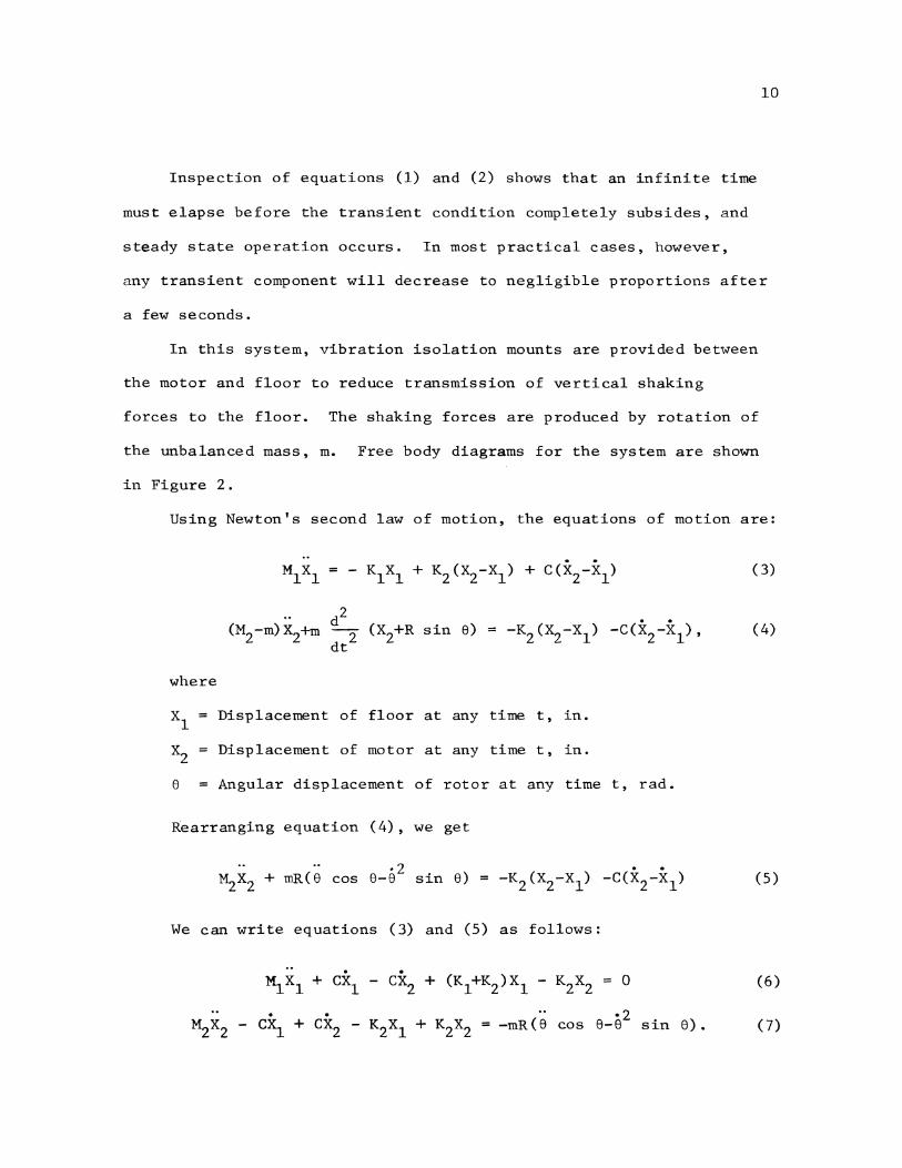
Inspection of equations (1) and (2) shows that an infinite time

must elapse before the transient condition completely subsides, and

steady state operation occurs. In most practical cases, however,

any transient component will decrease to negligible proportions after

a few seconds.

In this system, vibration isolation mounts are provided between

the motor and floor to reduce transmission of vertical shaking

forces to the floor. The shaking forces are produced by rotation of

the unbalanced mass, m. Free body diagrams for the system are shown

in Figure 2.

Using Newton's second law of motion, the equations of motion are:

Mlxl = - KlXl + K2 (X2-Xl) + C(X2-Xl) (3)

(M2-m) X2+m d2

(X2+R sin 8) -K2 (X2-Xl) -c(x2-x1), = dt2

(4)

where

xl Displacement of floor at any time t, in.

x2 Displacement of motor at any time t, in.

8 Angular displacement of rotor at any time t, rad.

Rearranging equation (4), we get

(5)

We can write equations (3) and (5) as follows:

(6)

(7)

11

Figure 2. Free Body Diagram of Forces Acting on System

12

The term on the right hand side of equation (7) represents the shaking

force produced by rotation of the unbalanced mass m, which is located

at the distance R from the centerline of the rotor. Let us describe

this force by the term f(t).

For a motor without an external load, the angular position of the

rotor at any time can be obtained from equation (1) or (2). However,

when the motor is coupled to an external load, 8(t) must be obtained

by solving the equation

T 0

I 8, 0

(8)

where

I = Moment of inertia of the rotor about center of rotation 0

excluding unbalanced mass m.

T Driving (electromotive) torque less the total load torque 0

about center of rotation.

In this thesis, T is specified as a function of w (see Appendix 0

B). Use of this relation in equation (8) permits the latter to be

solved for B(t), which is inserted in equation (7). Equations (6)

and (7) can then be solved on a digital computer for the displacements

x1 (t), x2 (t) and B(t) as discussed in Chapter IV.

Equations (6) and (7) can be written in matrix form as follows:

{0 } (9) f (t)

13

Let us define

(M] [; ~J [C) = [_: -: J [K) [Kl+K2 -K2]

-K K2 2

{X} {:) { f ( t)} L:t;

Now we can write equation (9) as follows:

[M]{X} + [C]{X} + [K]{X} { f ( t)} (10)

C. Derivation of Equations Considering Torque due to Vertical

Acceleration of Unbalanced Mass

Figure 3(a) shows the shaking forces and Figure 3(b) shows the

torques acting on the system when we take into consideration the effect

of "inertia torque" created by vertical acceleration x2 of the

unbalanced mass m. The net torque available for accelerating the

rotor is thus the electromotive torque less the total load torque,

which includes both the external load torque and the "inertia torque".

The equations of motion considering the effect of "inertia

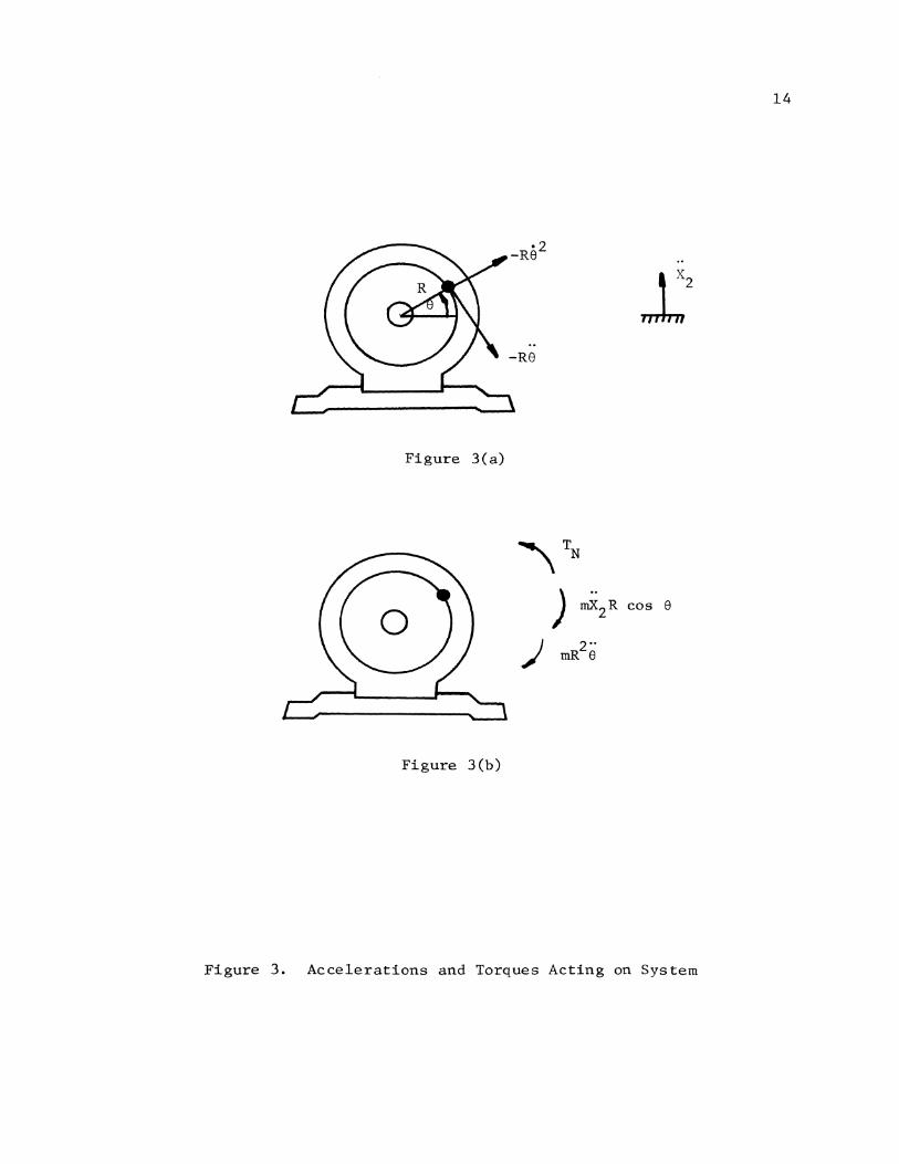
Figure 3(a)

)

Figure 3(b)

) mX2 R cos e

2 .. mR 8

Figure 3. Accelerations and Torques Acting on System

14

15

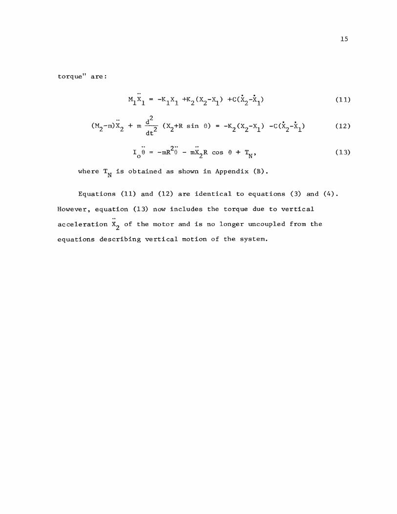
torque" are:

(11)

(12)

•• 2 •• I 0 6 = -mR 6- mX2R cos 8 +TN' (13)

where TN is obtained as shown in Appendix (B).

Equations (11) and (12) are identical to equations (3) and (4).

However, equation (13) now includes the torque due to vertical

acceleration x2 of the motor and is no longer uncoupled from the

equations describing vertical motion of the system.

16

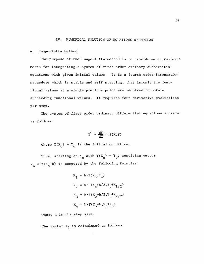
IV. NUMERICAL SOLUTION OF EQUATIONS OF MOTION

A. Runge-Kutta Method

The purpose of the Runge-Kutta method is to provide an approximate

means for integrating a system of first order ordinary differential

equations with given initial values. It is a fourth order integration

procedure which is stable and self starting, that is,only the func-

tional values at a single previous point are required to obtain

succeeding functional values. It requires four derivative evaluations

per step.

The system of first order ordinary differential equations appears

as follows:

' y = dY dX

= F(X,Y)

where Y(X ) = Y is the initial condition. 0 0

Thus, starting at X with Y(X ) = Y , resulting vector 0 0 0

Y(X +h) is computed by the following formulas: 0

Kl h•F(X ,Y ) 0 0

K2 h•F(X0 +h/2,Y 0 +Kl/Z)

K3 h•F(X0 +h/2,Y0 +KZ/Z)

K = 4 h•F(X +h,Y +K3)

0 0

where h is the step size.

The vector Y4 is calculated as follows:

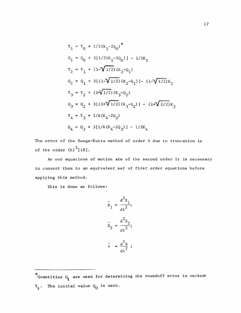
17

* yl Yo + 112 (K1-2Q0 )

Ql Qo + 3[1/2(K1-2Q0 )J l/2K1

y2 yl + (1--{lii.) (K2-Ql)

Q2 Ql + 3[(1-~(K2-Q1)]- (l-~K2

y3 y2 + (1-Vl/i) (K3-Q2)

Q3 Q2 + 3 [ (1+-{lii.) (K3-Q2)] - (l+l{li2)K3

y4 y3 + 1/6 (K4 -2Q3 )

Q4 = Q + 3

3[1/6(K4-2Q 3)] - l/2K4

The error of the Runge-Kutta method of order 4 due to truncation is

of the order (h) 5 [18].

As our equations of motion are of the second order it is necessary

to convert them to an equivalent set of first order equations before

applying this method.

This is done as follows:

d 2X 1

xl dt2 '

d 2X

x2 __ 2.

2 ' dt

e d2 e dt 2

* Quantities ~ are used for determining the roundoff error in vecto~

Yi. The initial value Q0 is zero.

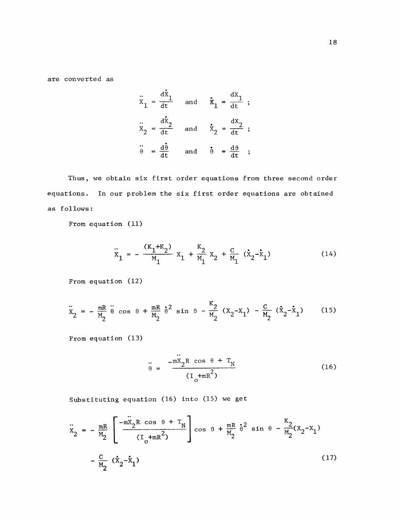
18

are converted as

. dX1 . dX1

xl dt and Kl dt

. dX2 . dX2

x2 = and x2 dt dt

. de . de

e and e = dt dt

Thus, we obtain six first order equations from three second order

equations. In our problem the six first order equations are obtained

as follows:

From equation (11)

From equation (12)

mR ·· + mR e·2 e cos e M2 M2

sin e

From equation (13)

e _mX2R cos e + TN

(I +mR2 ) 0

Substituting equation (16) into (15) we get

TN] cos e

(14)

(15)

(16)

sin

(17)

or

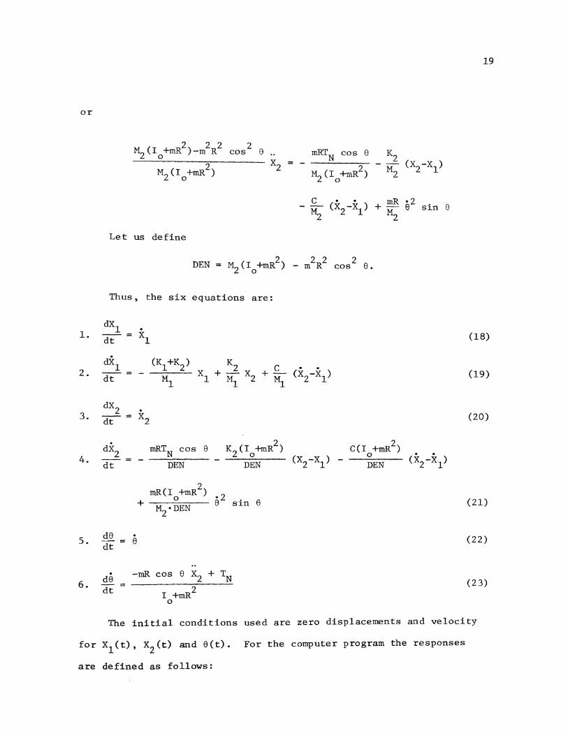
1.

2.

3.

4.

5.

6.

for

are

M (I +mR2)-m2R2 2 8 2 0

cos mRTN cos 8

M2(Io+mR2) x2 - -

M2 (Io+mR2)

c • • -- (X -X) ~ 2 1

Let us define

DEN = M2 (Io +mR2) - m2R2 2 e. cos

Thus, the six equations are:

dXl • d"t = xl

dXl (Kl+K2) K2 C • • dt = - Ml Xl + Ml X2 + ~ (X2-Xl)

d8 • dt = e

+

mRTN cos e

DEN

. -mR cos e x2 de -= dt I +mR2

0

sin e

+ TN

19

K2 (X2-Xl)

M2

+ mR •2 e sin 8 M2

(18)

(19)

(20)

(21)

(22)

(23)

The initial conditions used are zero displacements and velocity

x 1 (t), x 2 (t) and e(t). For the computer program the responses

defined as follows:

20

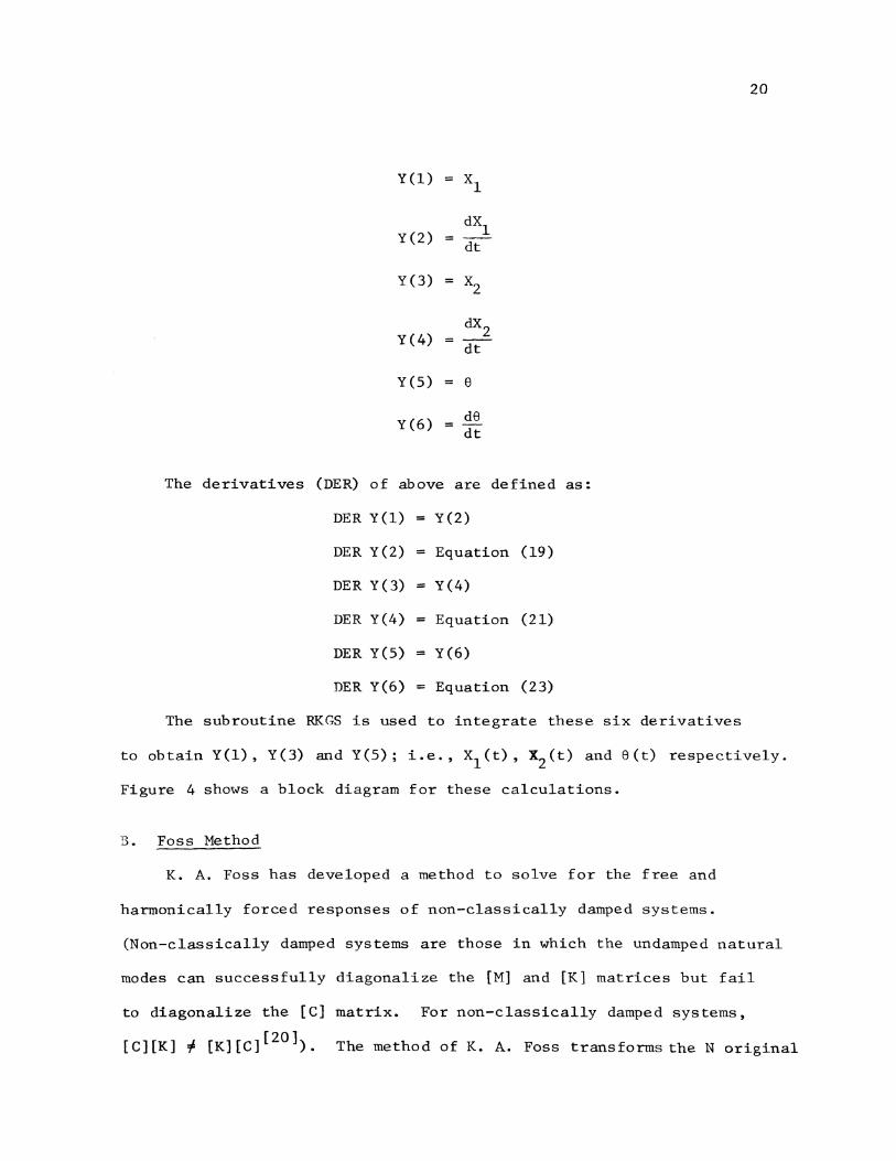
Y(l) xl

Y(2) dX1

= dt

Y(3) = x2

Y(4) dX2

= dt

Y(S) e

Y(6) de dt

The derivatives (DER) of above are defined as:

DER Y(l) = Y(2)

DER Y(2) = Equation (19)

DER Y(3) = Y(4)

DER Y(4) = Equation (21)

DER Y(S) = Y(6)

DER Y(6) = Equation (23)

The subroutine RKGS is used to integrate these six derivatives

to obtain Y(l), Y(3) and Y(S); i.e., x 1 (t), x2 (t) and 8(t) respectively.

Figure 4 shows a block diagram for these calculations.

B. Foss Method

K. A. Foss has developed a method to solve for the free and

harmonically forced responses of non-classically damped systems.

(Non-classically damped systems are those in which the undamped natural

modes can successfully diagonalize the [M) and [K] matrices but fail

to diagonalize the [C] matrix. For non-classically damped systems,

[C][K] .f; [K][C] [ 20]). The method of K. A. Foss transforms the N original

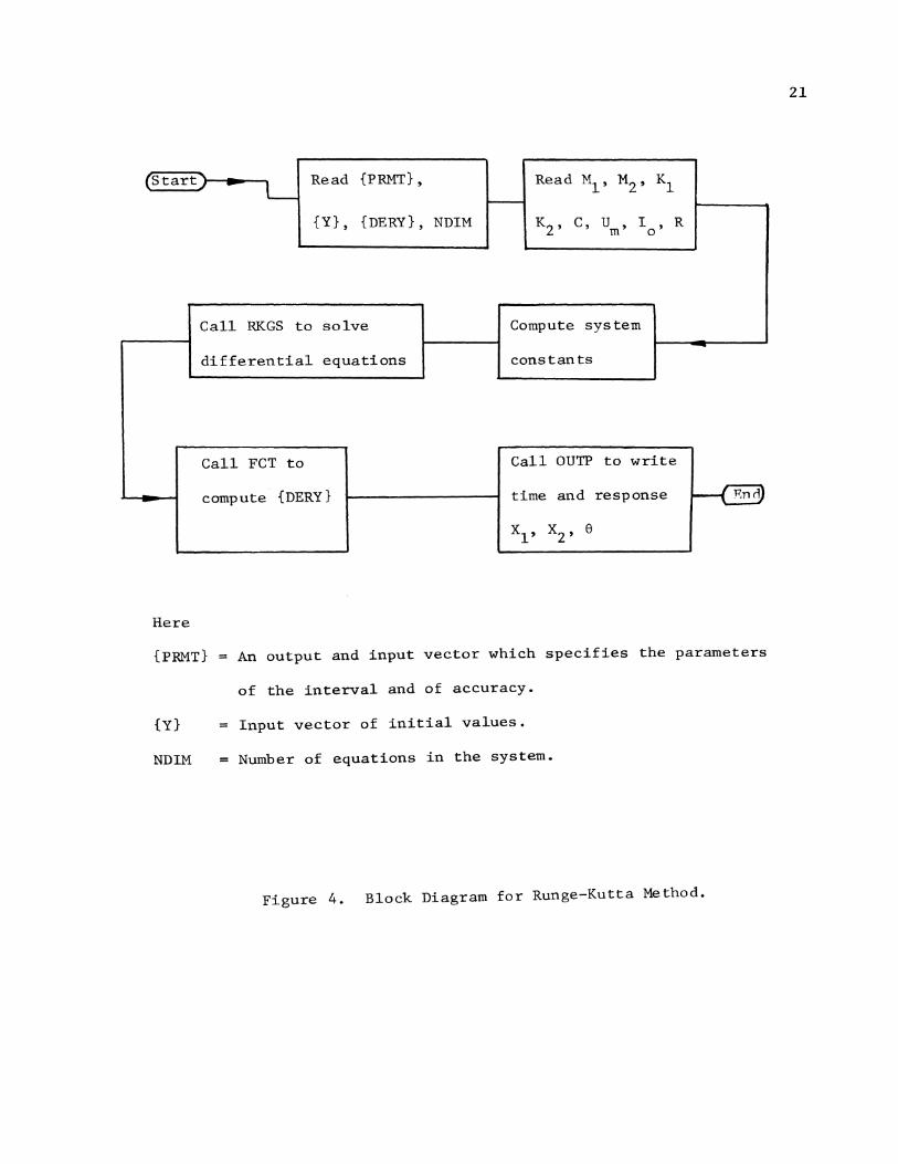
(Startj .. L Read {PRMT}, Read M1 , M2' Kl

~

{Y}, {DERY}, NDIM K2' c, u m' I ' R 0

Call RKGS to solve Compute sys tern

differential equations constants

Call FCT to Call OUTP to write

compute {DERY} time and response ---cB Xl, X2, 8

Here

{PRMT} An output and input vector which specifies the parameters

of the interval and of accuracy.

{Y}

NDIM

Input vector of initial values.

= Number of equations in the system.

Figure 4. Block Diagram for Runge-Kutta Method.

21

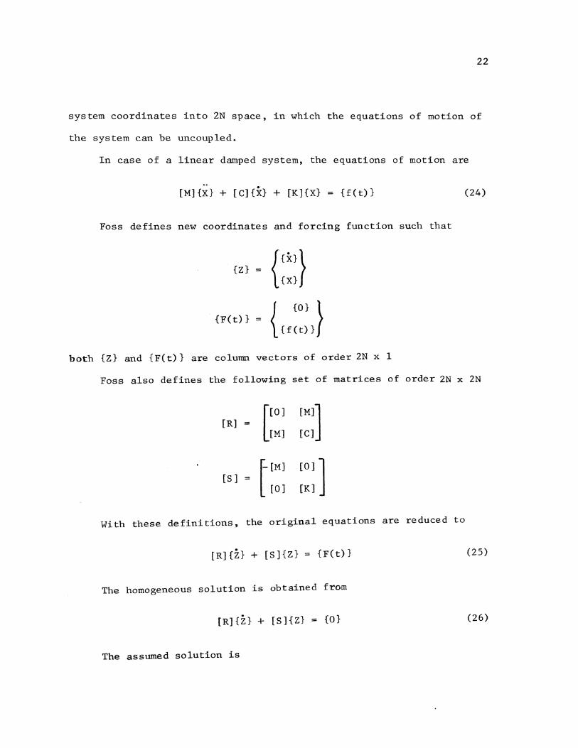
22

system coordinates into 2N space, in which the equations of motion of

the system can be uncoupled.

In case of a linear damped system, the equations of motion are

[M]{X} + [C]{X} + [K]{X} { f ( t)} (24)

Foss defines new coordinates and forcing function such that

{Z} {{x}} {X}

{ {0} }

{ f ( t)} {F(t)}

both {Z} and {F(t)} are column vectors of order 2N x 1

Foss also defines the following set of matrices of order ZN x 2N

[R] [[0]

[M]

[M]] [C]

l [M] [S] =

[0]

[0]] [K]

With these definitions, the original equations are reduced to

[R]{Z} + [S]{Z} {F(t)} (25)

The homogeneous solution is obtained from

[R]{Z} + [S]{Z} = {0} (26)

The assumed solution is

23

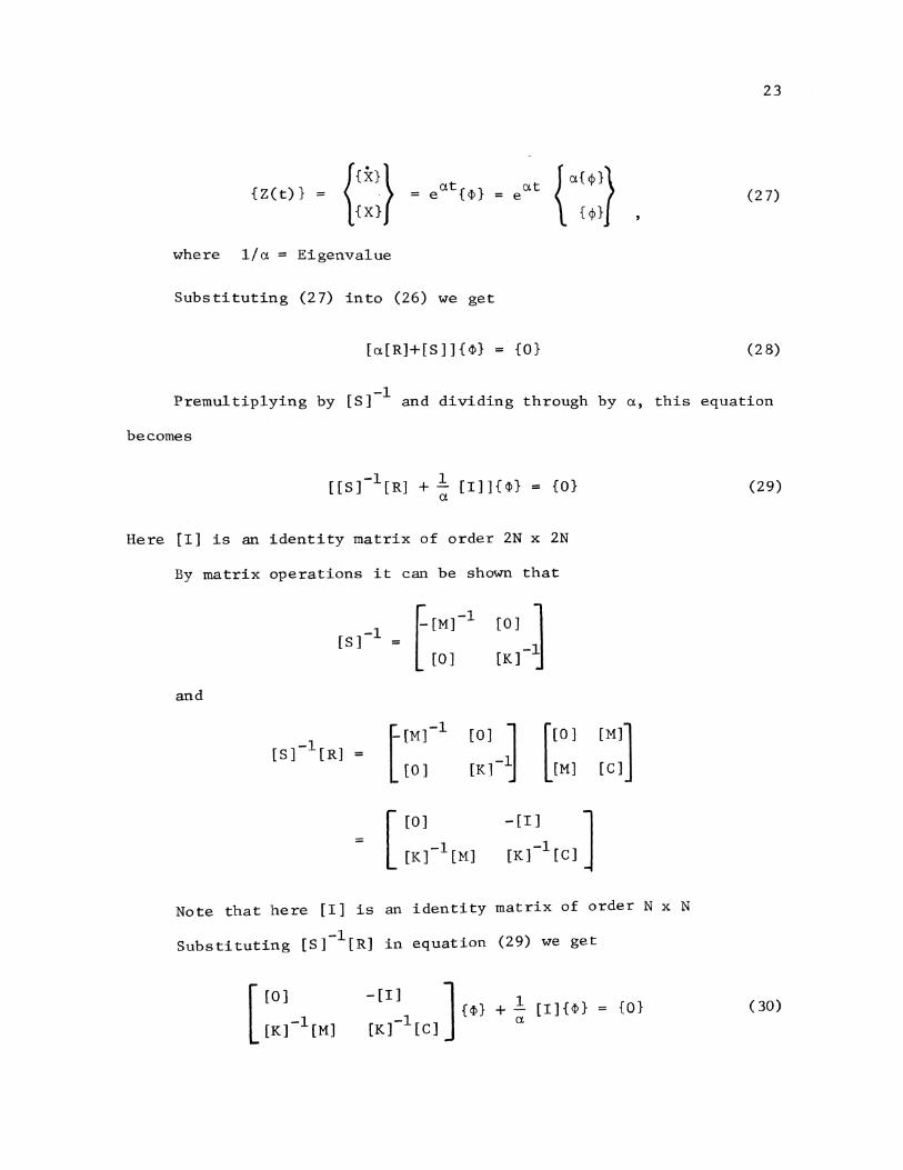
r}} eat{<P} at {"{4}} {Z(t)} = e {X} {ljl}

(2 7)

where 1/a = Eigenvalue

Substituting (27) into (26) we get

[a[R]+[S]]{<P} = {0} (2 8)

Premultiplying by [S]-l and dividing through by a, this equation

becomes

[[S]-1 [R] + ~ [I]]{<P} = {0} a

Here [I] is an identity matrix of order 2N x 2N

By matrix operations it can be shown that

and

-1 f[M]-1 [S] =

[0]

[0] l [K]-lJ

r-[M]-1

L ro]

[O] l [K]-lJ

[[0]

[M]

= [ [O]

[K]-l[M]

-[I] ]

[K]-l[C]

[M]] [C]

Note that here [I] is an identity matrix of order N x N

-1 Substituting [S] [R] in equation (29) we get

-[I] J {<P} + ~ [I){<P} [K]-l[C] a

{0}

(29)

( 30)

24

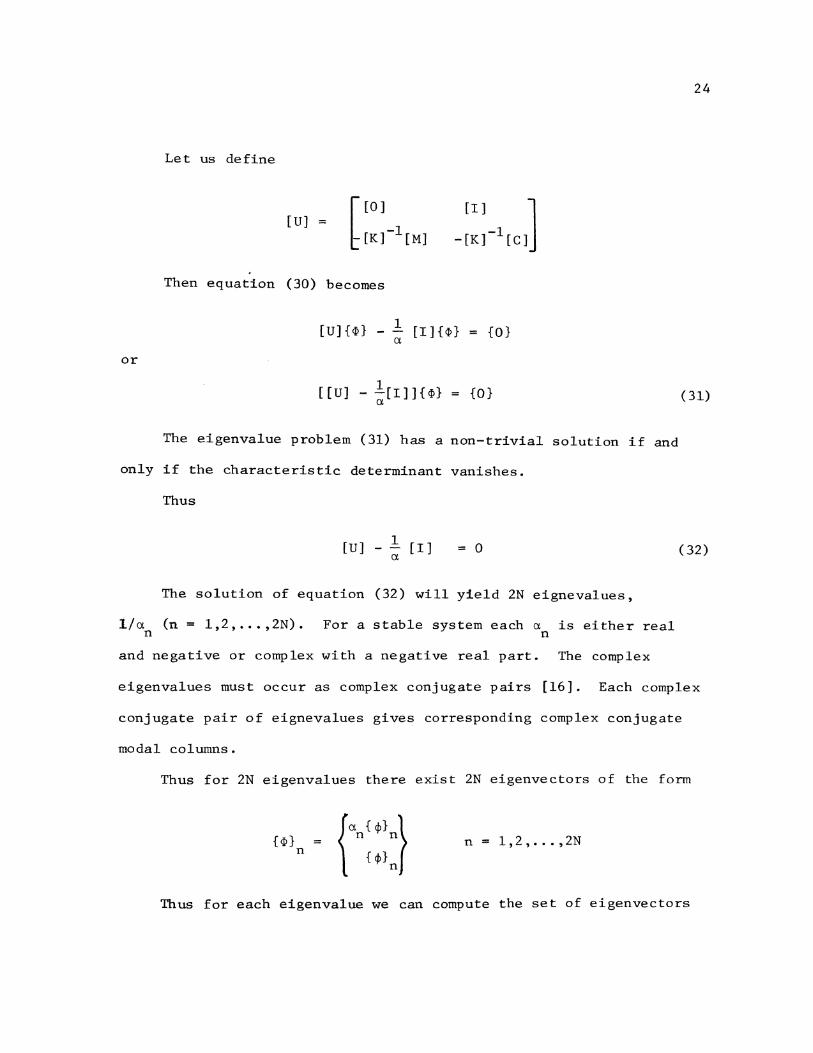
Let us define

[U]

Then equation (30) becomes

[U]{~} - l [I]{~} = {0} a

or

[[U] _ _l[I]]{~} a

{0} (31)

The eigenvalue problem (31) has a non-trivial solution if and

only if the characteristic determinant vanishes.

Thus

[U] - l [I] a = 0 (32)

The solution of equation (32) will yield 2N eignevalues,

1/a (n = 1,2, ... ,2N). For a stable system each a is either real n n

and negative or complex with a negative real part. The complex

eigenvalues must occur as complex conjugate pairs [16]. Each complex

conjugate pair of eignevalues gives corresponding complex conjugate

modal columns.

Thus for 2N eigenvalues there exist 2N eigenvectors of the form

{~} n

n 1, 2 , •.. , 2N

Thus for each eigenvalue we can compute the set of eigenvectors

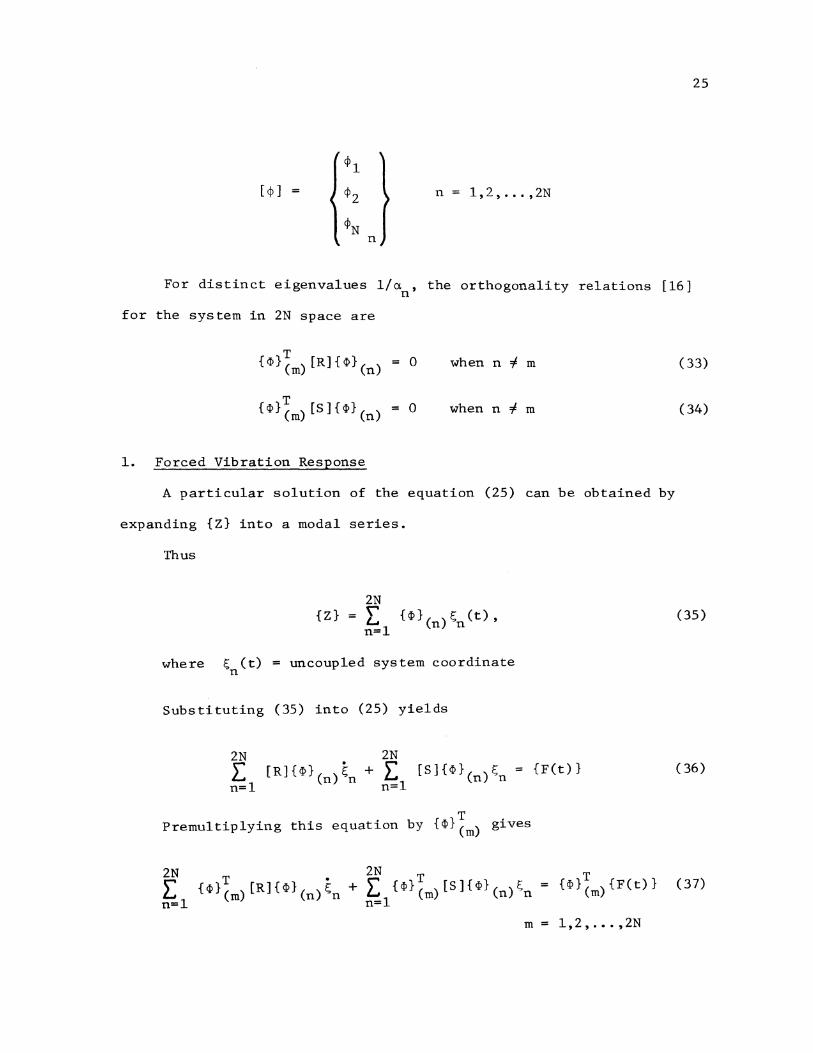
25

[<jl] n = 1, 2, •.. , 2N

n

For distinct eigenvalues 1/a , the orthogonality relations [16] n

for the system in 2N space are

T {ci>}(m) [R]{ci>}(n) 0 when n =f. m

T { ci> } ( m) [ S ]{ ci>} ( n) 0 when n =f. m

1. Forced Vibration Response

A particular solution of the equation (25) can be obtained by

expanding {Z} into a modal series.

Thus

2N {Z} L {ci>} (n) ~n (t)'

n=l

where ~ (t) = uncoupled system coordinate n

Substituting (35) into (25) yields

T Premultiplying this equation by {ci>}(m) gives

{F(t)}

{ci>}~m){F(t)}

m = 1, 2, .•. , 2N

(33)

(34)

(35)

(36)

(37)

26

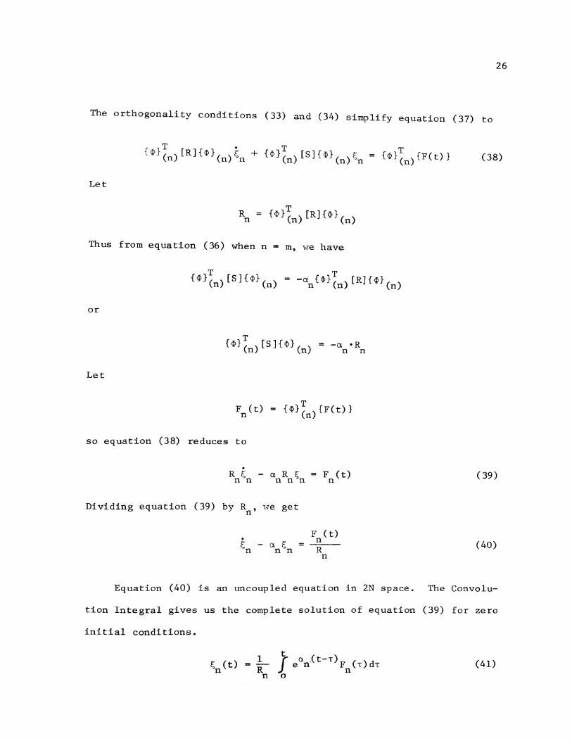
The orthogonality conditions (33) and (34) simplify equation (37) to

Let

R n T

{ <P} (n) [R]{ <P} (n)

Thus from equation (36) when n = m, v-1e have

T {<P} (n) [S){<P} (n)

or

T { <P} (n) [S ]{ <P} (n)

Let

so equation (38) reduces to

. R i; - a R i;

n n n n n

Dividing equation (39) by R , ~ve get n

. i; - a i; n n n

-a •R n n

F (t) n

F (t) n R

n

T {<P} (n) {F(t)} (38)

(39)

(40)

Equation (40) is an uncoupled equation in 2N space. The Convolu-

tion Integral gives us the complete solution of equation (39) for zero

initial conditions.

1 i; (t) = n R

n (41)

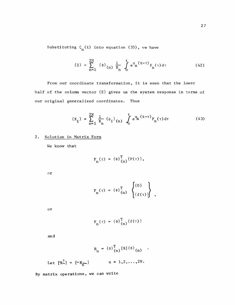
Substituting t;. (t) into equation (35), we have n

{Z}

From our coordinate transformation, it is seen that the lower

27

(42)

half of the column vector {Z} gives us the system response in terms of

our original generalized coordinates. Thus

2N t {Xi} E 1

{<jli}(n) J e a.n ( t-T) Fn (L) dT ( 43) = R n=l n 0

2. Solution in Matrix Form

We know that

F (T) n

T {<I>}(n){F(T)},

or

T fO} } F (T) {<I>}(n) n {f(T)} '

or

F ( T) n

T {<I>}(n){f(T)}

and

R {<I>}~n) [R]{<I>}(n) n

Let [·R!] = [-R-] n = 1, 2 , .•• , 2N. n

By matrix operations, we can write

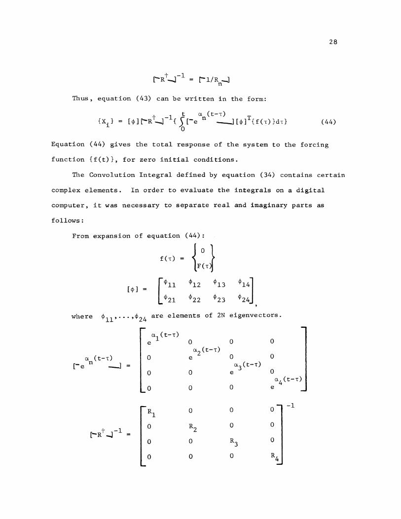
28

Thus, equation (43) can be written in the form:

(44)

Equation (44) gives the total response of the system to the forcing

function {f(t)}, for zero initial conditions.

The Convolution Integral defined by equation (34) contains certain

complex elements. In order to evaluate the integrals on a digital

computer, it was necessary to separate real and imaginary parts as

follows:

From expansion of equation ( 44):

f(T) {F:T} [cp] [•u cpl2 ¢13 .14]

<Pzl <Pzz <Pz3 <Pz4

where <P11'···•<Pz4 are elements of 2N eigenvectors.

a.1 (t-T) 0 0 0 e

a. (t-T) 0 a.2 (t-T)

0 0 e [-en -l a.3 (t-T)

0 0 0 e

0 a 4 (t-T)

0 0 e

0 0 -1

Rl 0

0 R2 0 0 [-Rt -J-1

0 0 R3 0

0 0 0 R4

29

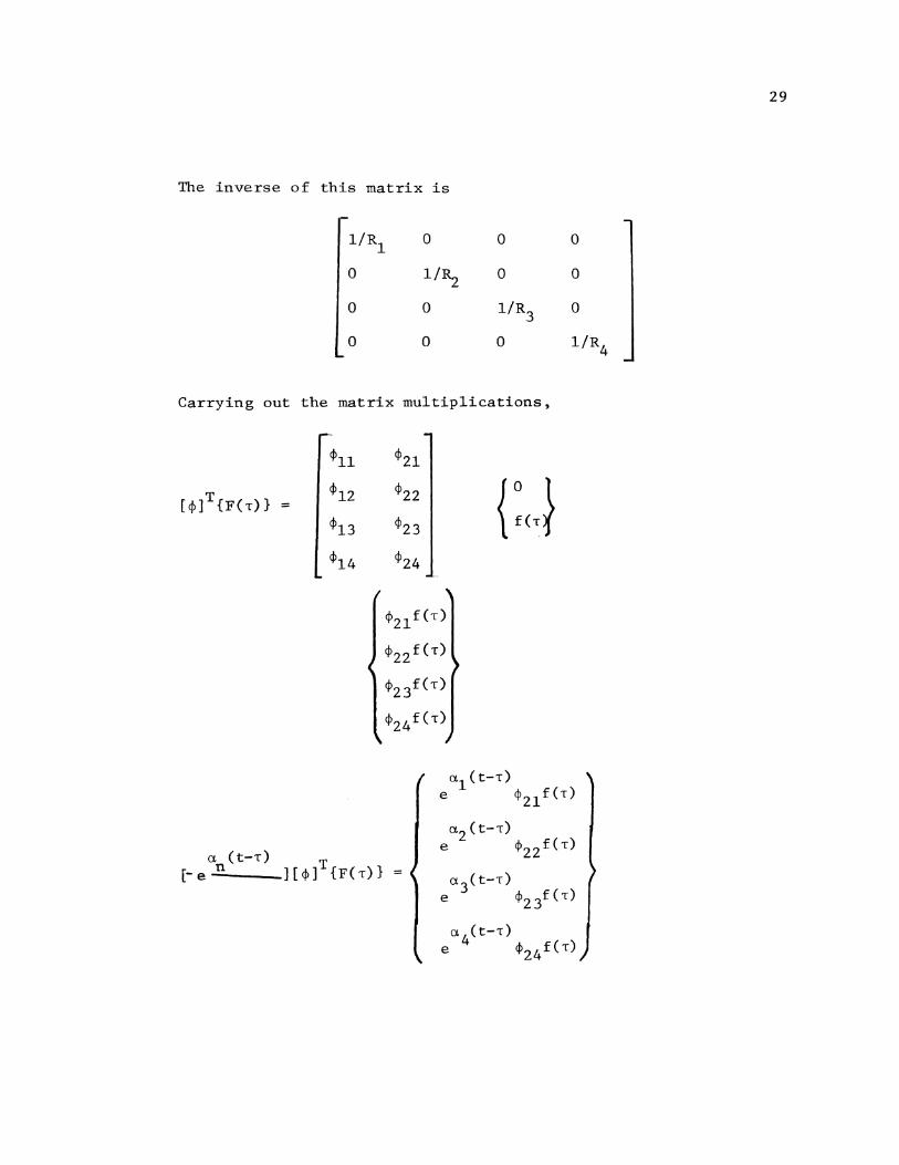
The inverse of this matrix is

l/R1 0 0 0

0 1/~ 0 0

0 0 l/R3 0

0 0 0 l/R4

Carrying out the matrix multiplications,

<1>11 <1>21

[<j>]T{F(T)} <1>12 <~>22

= <1>13 <1>23

<1>14 <1>24

a.1 (t-T) e cp 21 f(T)

a.2 (t-T) e cp 22 f(T)

a. 3 (t-T) e ¢23f(T)

a. 4(t-T) e <1>z4f(<)

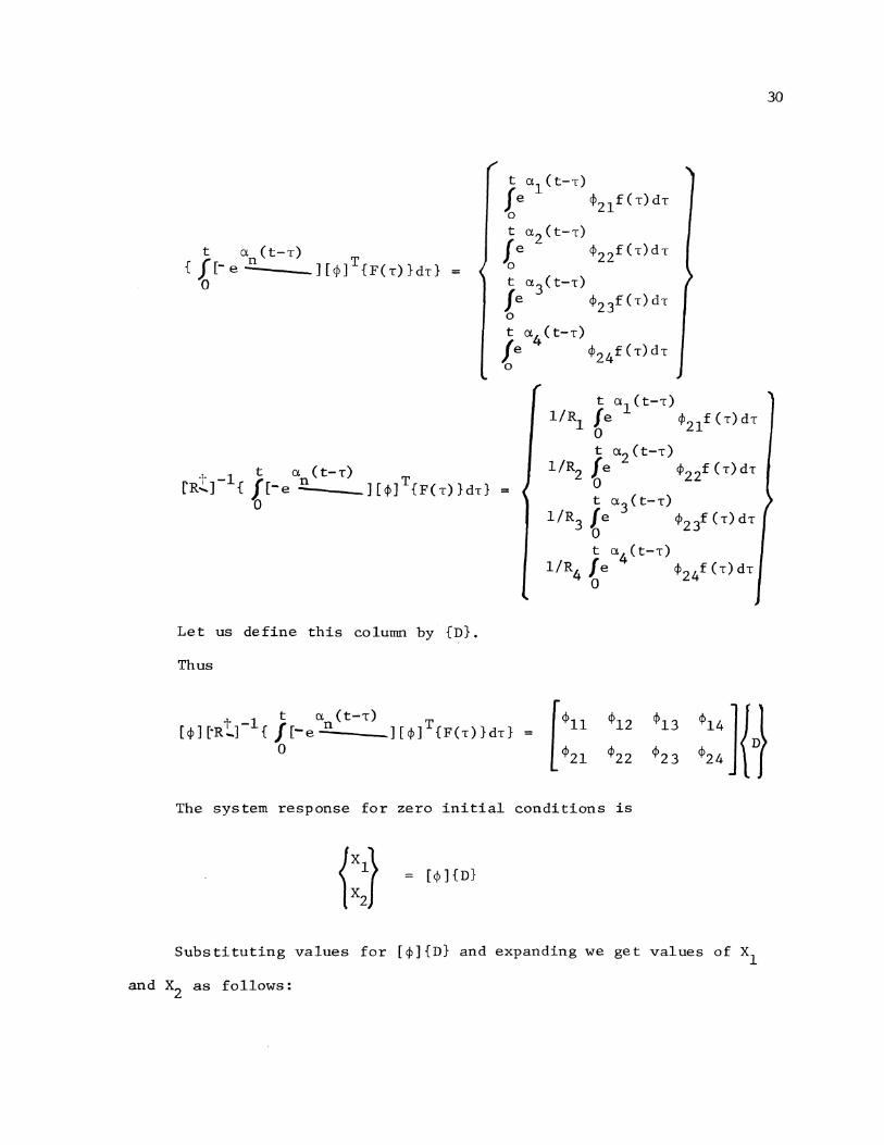
t a.l ( t--r) Je $2lf(-r)d-r 0

t a.2 Ct--r) [e $22f(-r)d-r 0

t a.3 (t-T) Je $23f(-r)d-r 0

t a.4(t--r) fe ~24f(-r)d-r 0

Let us define this column by {D}.

Thus

t Cl. (t-T) [ •u $12 $13

:::JH [cj>][·R!.J-1 { fe-e n T ][cj>] {F(-r)}d-r} = 0 $21 4>22 4>23

The system response for zero initial conditions is

[cj>]{D}

Substituting values for [cj>]{D} and expanding we get values of x1

and x2 as follows:

30

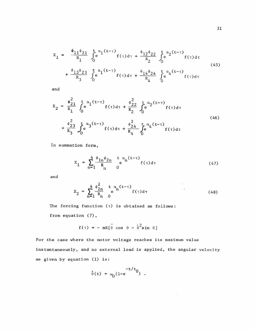
<Pll<P21 t a 1 (t-T) <Pl2<P22 t a 2 (t-T)

xl Rl

fe f(T)dT + ,[e f(T)dT 0 R2 0

<Pl3<P23 t a 1 (t-T) <Pl4<P24 t a 4 (t-T)

+ _[ e f(T)dT + fe f(T)dT R3 R4 0 0

and

2 <P24 ~ a4 ( t-T) -R---~e f(T)dT

In summation form,

and

4 0

t a (t-T) n

e f(T)dT 0

t a (t-T) n

e f(T)dT 0

The forcing function (T) is obtained as follows:

from equation (7),

.. . 2 f(T) = - mR(8 cos 8 - 8 sin 8]

For the case where the motor voltage reaches its maximum value

31

(45)

(46)

(47)

(48)

instantaneously, and no external load is applied, the angular velocity

as given by equation (1) is:

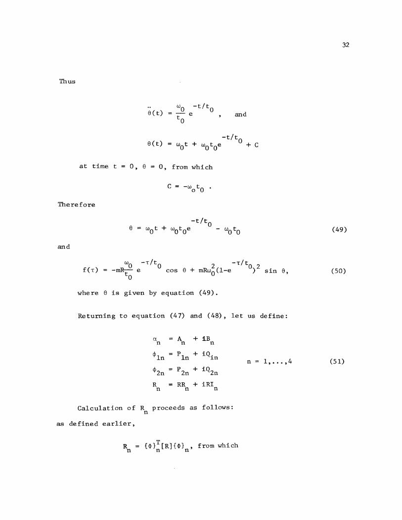
Thus

at time t

Therefore

and

f(T)

o, e

e

e c t) -t/t

0 e

0, from which

where e is given by equation (49).

and

Returning to equation (47) and (48), let us define:

a = A + iB n n n

<j>ln pln + iQ. ~n

<j>2n p2n + iQ2n

R RR + iRI n n n

Calculation of R proceeds as follows: n

as defined earlier,

R {~}T[R]{~} , from which n n n

n=l, •.• ,4

32

(49)

(50)

(51)

33

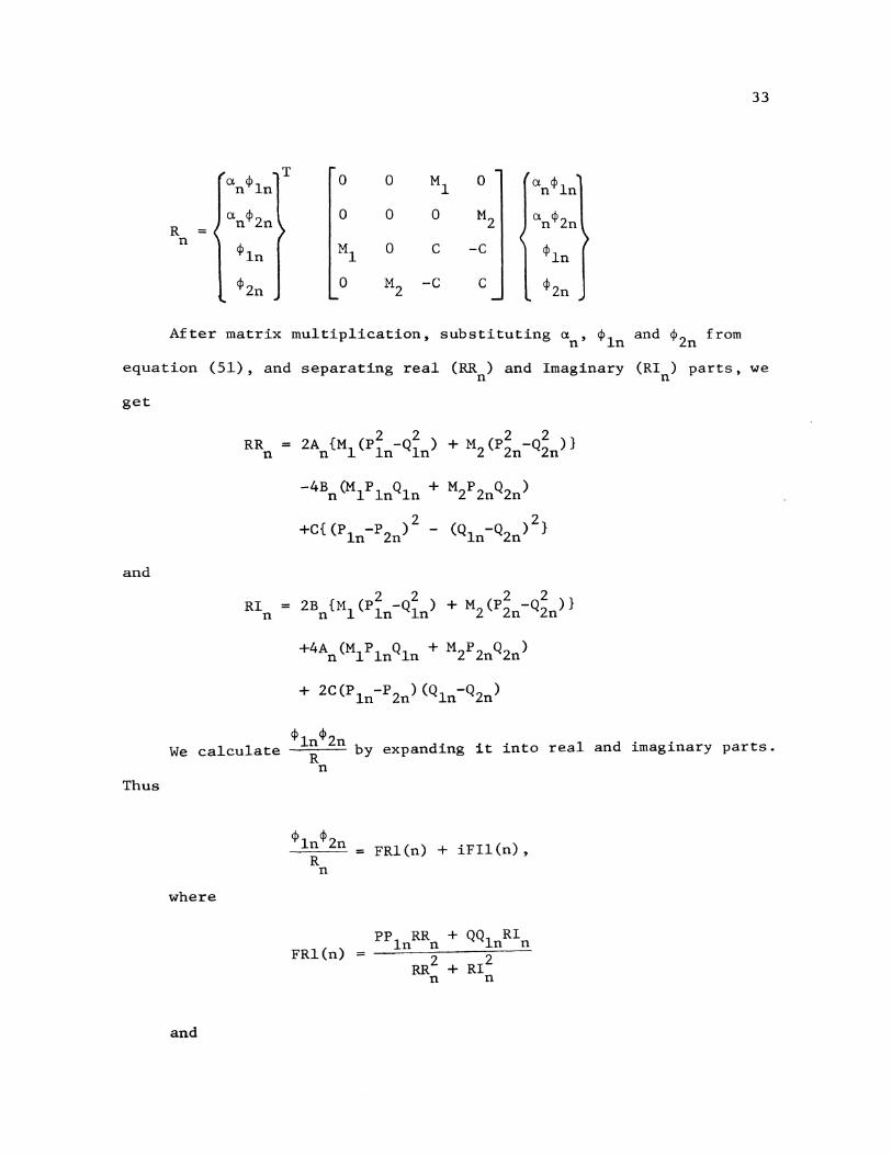
a.n<Pln T

0 0 Ml 0 a.n<Pln

a.n<P2n 0 0 0 M2 a.n<P2n R = n

<Pln Ml 0 c -c <Pln

<P2n 0 M2 -c c <P2n

After matrix multiplication, substituting a. , <Pln and <P 2n from n

equation (51), and separating real (RR) and Imaginary (RI) parts, we n n

get

and

Thus

RR n

RI n

- 4Bn(MlPlnQln + M2P2nQ2n)

2 2 +C{(Pln-P2n) - (Qln-Q2n) }

<P ln <P2n We calculate R by expanding it into real and imaginary parts.

where

and

n

<Pln<P2n R

n

= FRl(n) + iFil(n),

FRl(n) = pplnRRn + QQlnR1n

RR2 + RI2 n n

Fil(n)

with

and

QQl RR n n - RI PP1 n n

p p - Q Q ln 2n ln 2n

Qlnp2n + PlnQ2n

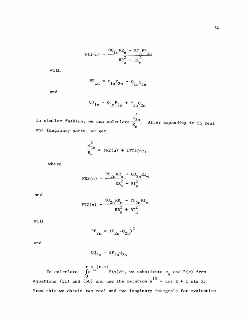
34

In similar fashion, we can calculate

2 <l>zn R" After expanding it in real

n and imaginary parts, we get

where

and

with

and

To calculate

equations (51) and

2 <l>zn --= R

n

FR2(n)

FI2(n) =

FR2(n) + iFI2(n),

pp2 RR n n

QQ2 RR n n

+ QQ2 RI n n

- pp RI 2n n

t a (t-T) fe n F(T)dT, we substitute an and F(T) from o ·x

(50) and use the relation e 1 = cos X + i sin X.

From this we obtain two real and two imaginary integrals for evaluation

35

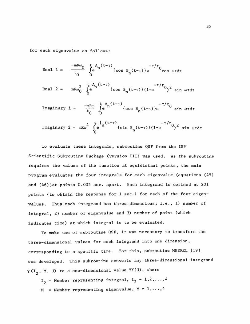
for each eigenvalue as follows:

-mRw t A (t-T) -T/t 0 Real 1 fe n {cos B (t-T)}e 0 WTdT

to cos

0 n

mRw2 t A (t-T) -T/t

Real 2 = J e n . {cos B (t-T)}(l-e 0 ) 2 sin WTdT 0 0 n

-mRw t A (t-T) -T/t Imaginary 1 J e n {cos B (t-T)}e 0

to sin WTdT

0 n

2 t ( (t-T) -T/tQ 2 Imaginary 2 = mRw [ e n {sin B ( t-T)} (1-e ) sin wTdT

0 n

To evaluate these integrals, subroutine QSF from the IBM

Scientific Subroutine Package (version III) was used. As the subroutine

requires the values of the function at equidistant points, the main

program evaluates the four integrals for each eigenvalue (equations (45)

and (46))at points 0.005 sec. apart. Each integrand is defined at 201

points (to obtain the response for 1 sec.) for each of the four eigen-

values. Thus each integrand has three dimensions; i.e., 1) number of

integral, 2) number of eigenvalue and 3) number of point (which

indicates time) at which integral is to be evaluated.

To make use of subroutine QSF, it was necessary to transform the

three-dimensional values for each integrand into one dimension,

corresponding to a specific time. For this, subroutine MERREL [19]

was developed. This subroutine converts any three-dimensional integrand

y (I 2 , M, J) to a one-dimensional value YY (J), Hhere

r 2 Number representing integral, r 2 = 1,2, .•. ,4

M Number representing eigenvalue, M = 1, ... ,4

J =Number representing time interval, J = 1,2, •.• ,201

Subroutine QSF is now used to calculate ZZ(J), integrated value of

YY(J), up to time J. Subroutine MERREL now transforms the one-

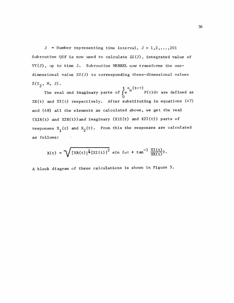
dimensional value ZZ(J) to corresponding three-dimensional values

Z(I2 , M, J). t a (t-T)

The real and imaginary parts of fen F(c)dT are defined as 0

ZR(t) and ZI(t) respectively. After substituting in equations (47)

and (48) all the elements as calculated above, we get the real

(XlR(t) and X2R(t))and imaginary (Xll(t) and X2I(t)) parts of

responses x1 (t) and x2 (t). From this the responses are calculated

as follows:

X(t) ~[XR(t)J~[XI(t)] 2 sin -1 XI(t)

(wT +tan XR(t)).

A block diagram of these calculations is shown in Figure 5.

36

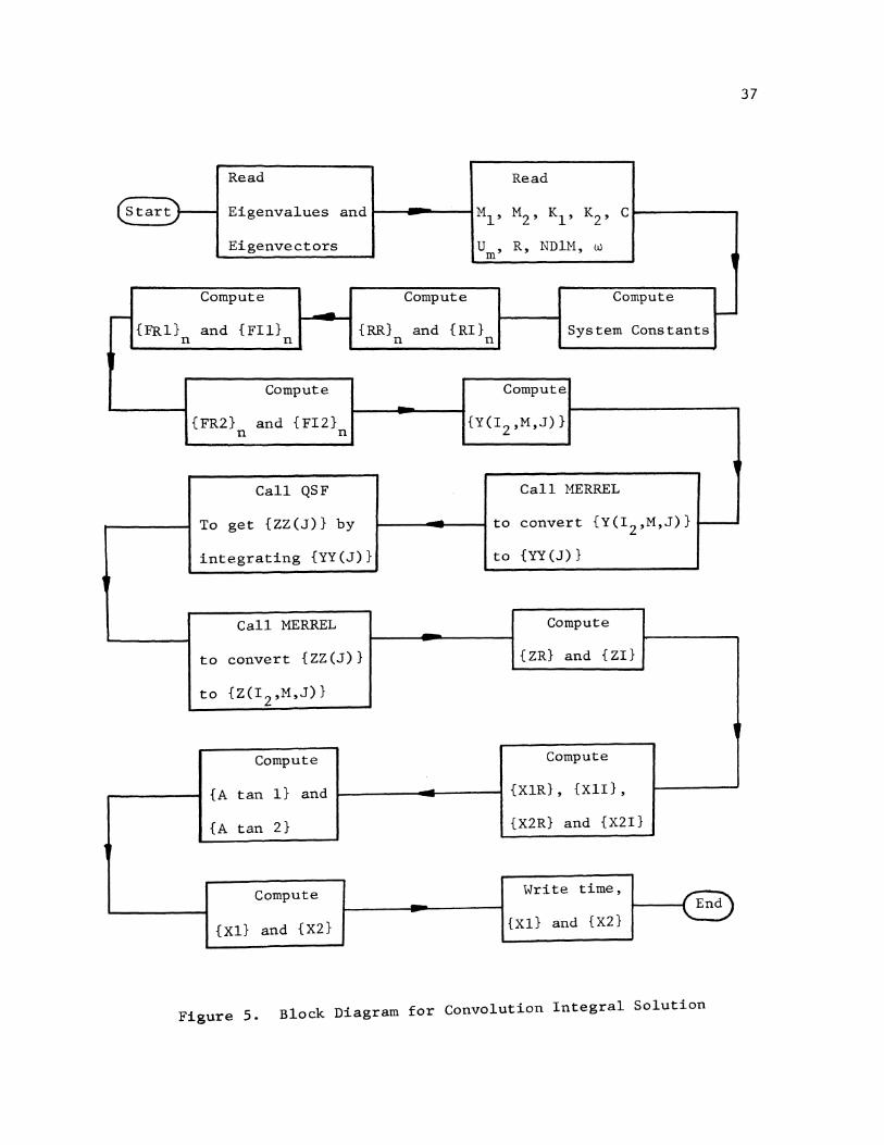
37

Read Read

(start)-- Eigenvalues and Ml, M2' Kl, K2' c

Eigenvectors u ' m R, NDlM, w

' Compute Compute Compute

.-- - 1--{FR.l} and {Fil} {RR} and {RI} System Constants

n n n n

Compute Compute

{FR2} and {FI2} {Y(I2 ,M,J)} n n

1

Call QSF Call MERREL

To get {ZZ(J)} by to convert {Y(I2 ,M,J)}

integrating {YY(J)} to {YY (J)}

Call MERREL Compute -to convert {ZZ(J)} {ZR} and {ZI}

to {Z(I 2 ,M,J)}

' Compute Compute

{A tan 1} and {XlR}, {Xli},

{A tan 2} {X2R} and {X2I}

Compute Write time,

- End

{Xl} and {X2} {Xl} and {X2}

Figure s. Block Diagram for Convolution Integral Solution

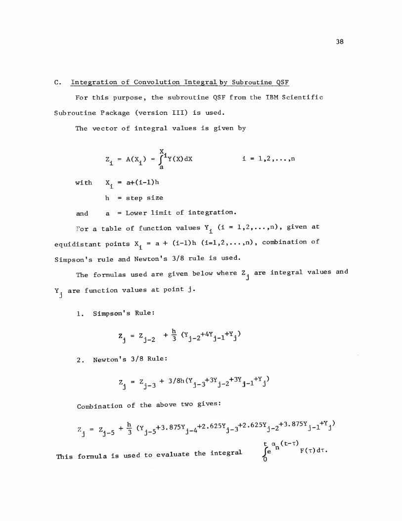
C. Integration of Convolution Integral by Subroutine QSF

For this purpose, the subroutine QSF from the IBM Scientific

Subroutine Package (version III) is used.

The vector of integral values is given by

with

z. 1.

X. A(Xi) = J1 Y(X)dX

a

xi = a+(i-l)h

h = step size

and a = Lower limit of integration.

i = 1,2, ••• ,n

For a table of function values Y. (i = 1,2, ••• ,n), given at 1.

equidistant points X.= a+ (i-l)h (i=l,2, ••• ,n), combination of 1.

Simpson's rule and Newton's 3/8 rule is used.

38

The formulas used are given below where Z. are integral values and J

Y. are function values at point j. J

1. Simpson's Rule:

Z. = Z. 2 + h3 (Y. 2+4Y. 1+Y.) J J- J- J- J

2. Newton's 3/8 Rule:

Combination of the above two gives:

+ h (Y +3 875Y +2.625Y 3+2.625Y. 2+3.875Y. 1+Y.) zj zj-5 3 j-5 . j-4 j- J- J- J

t a. ( t-T) Je n F(T)dT. 0

This formula is used to evaluate the integral

39

V. APPLICATION TO PRACTICAL VIBRATION ISOLATION SYSTEM

As indicated earlier the primary objectives of this thesis are

to develop practical methods for calculating the transient responses

of systems with vibration isolation, and to apply these methods to

typical cases. In the examples that follow, transient and steady state

responses are compared, and the influence of inertia torque on system

behavior is illustrated.

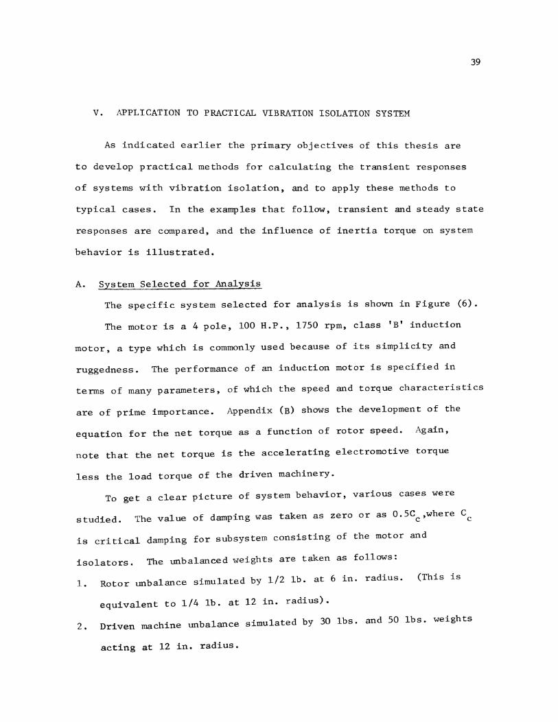
A. System Selected for Analysis

The specific system selected for analysis is shown in Figure (6).

The motor is a 4 pole, 100 H.P., 1750 rpm, class 'B' induction

motor, a type which is commonly used because of its simplicity and

ruggedness. The performance of an induction motor is specified in

terms of many parameters, of which the speed and torque characteristics

are of prime importance. Appendix (B) shows the development of the

equation for the net torque as a function of rotor speed. Again,

note that the net torque is the accelerating electromotive torque

less the load torque of the driven machinery.

To get a clear picture of system behavior, various cases were

studied. The value of damping was taken as zero or as 0.5Cc,where Cc

is critical damping for subsystem consisting of the motor and

isolators. The unbalanced weights are taken as follows:

1. Rotor unbalance simulated by 1/2 lb. at 6 in. radius.

equivalent to 1/4 lb. at 12 in. radius).

(This is

2. Driven machine unbalance simulated by 30 lbs. and 50 lbs. -.;.;reights

acting at 12 in. radius.

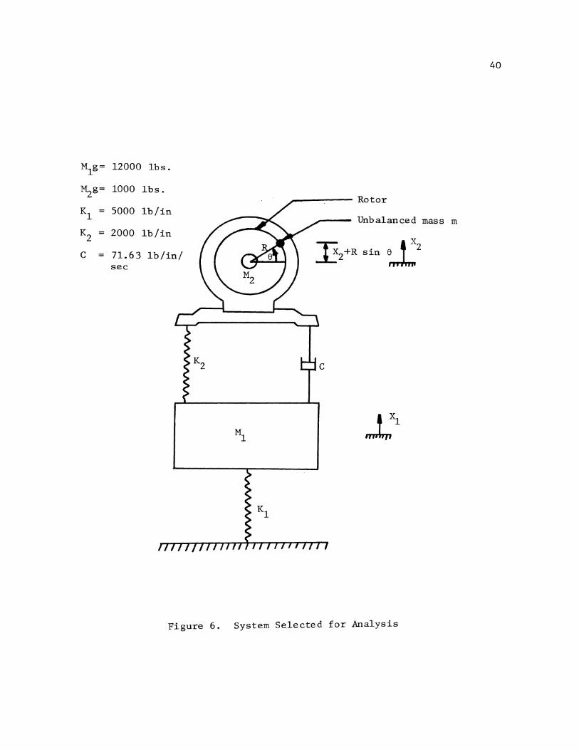
40

M g= 1

12000 lbs.

~g= 1000 lbs. Rotor

Kl 5000 lb/in Unbalanced mass m

K2 2000 lb/in

c 71.63 lb/in/ ~2+R sin ~2 sec

Figure 6. System Selected for Analysis

41

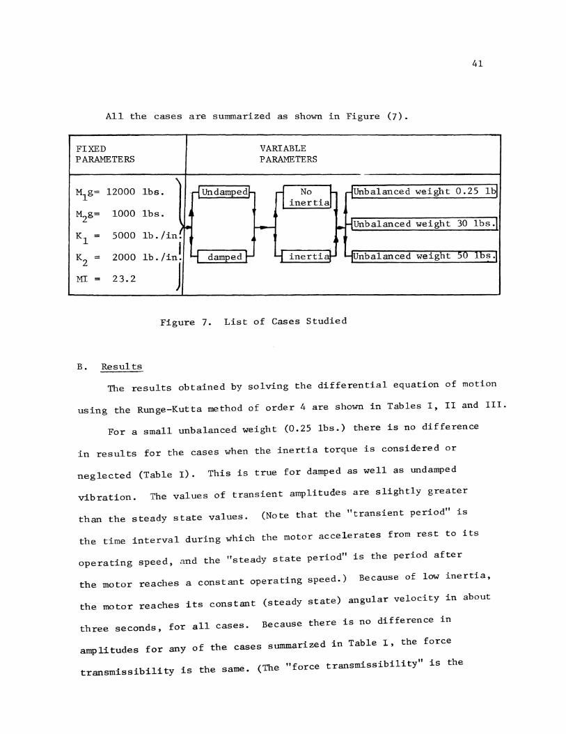
All the cases are summarized as shown in Figure (7).

FIXED VARIABLE PARAMETERS PARAMETERS

...

M g= 1

12000 lbs. -~ Undampedl- ri in:~tiJ r{Unbalanced weight 0.25 lbj

M g= 1000 lbs. 2

j

• f.- 1- Hunbalanced weight 30 lbs ~

Kl = 5000 lb. /in!

K2 = 2000 lb. /in! L.f dampedl- ~ inert{aj- fUnbalanced weight 50 lbs-:)

MI = 23.2 J

Figure 7. List of Cases Studied

B. Results

The results obtained by solving the differential equation of motion

using the Runge-Kutta method of order 4 are shown in Tables I, II and III.

For a small unbalanced weight (0.25 lbs.) there is no difference

in results for the cases when the inertia torque is considered or

neglected (Table I). This is true for damped as well as undamped

vibration. The values of transient amplitudes are slightly greater

than the steady state values. (Note that the "transient period" is

the time interval during which the motor accelerates from rest to its

operating speed, and the "steady state period" is the period after

the motor reaches a constant operating speed.) Because of low inertia,

the motor reaches its constant (steady state) angular velocity in about

three seconds, for all cases. Because there is no difference in

amplitudes for any of the cases summarized in Table I, the force

transmissibility is the same. (The "force transmissibility" is the

42

ratio of the force transmitted by spring K to the unbalanced shaking

force.)

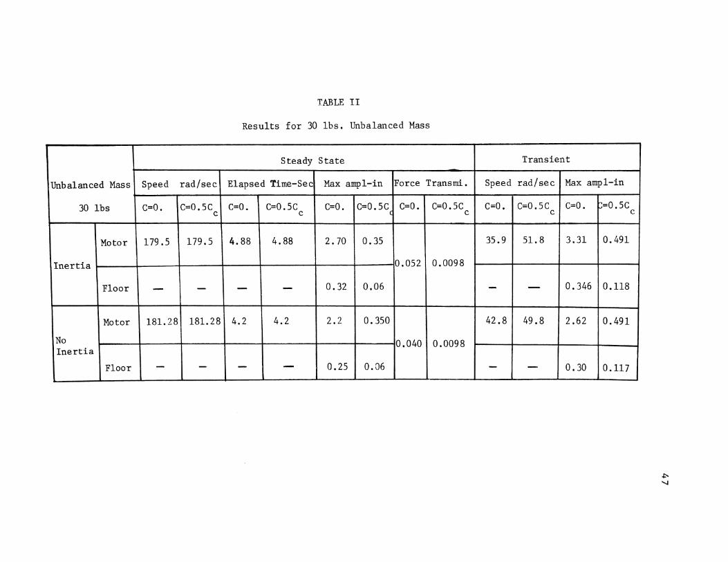
For an unbalanced mass weighing 30 lbs., we observe significant

differences in transient as well as steady state responses, for cases

without damping, when the inertia torque is first considered and then

neglected (Table II). However, when damping is present, the inertia

torque has no effect on system response. This is because damping

reduces the vertical displacement and minimizes the inertia torque

produced by the vertical acceleration of the unbalanced mass. The

transient amplitudes are greater than the steady state amplitudes, but

when damping is present the difference is significantly less. The

motor reaches its steady state speed (181.28 rad./sec.) in about 4

seconds when the effect of inertia torque is not considered. When

inertia torque is included, the motor reaches 99% of its steady state

value in about 4.8 seconds but varies thereafter about 178 rad./sec.

and 181 rad./sec. in damped and undamped cases respectively. The force

transmissibilities are identical for the damped inertia and no inertia

cases. However, for the undamped cases force transmissibility is

greater when the inertia torque is considered. To show the differences

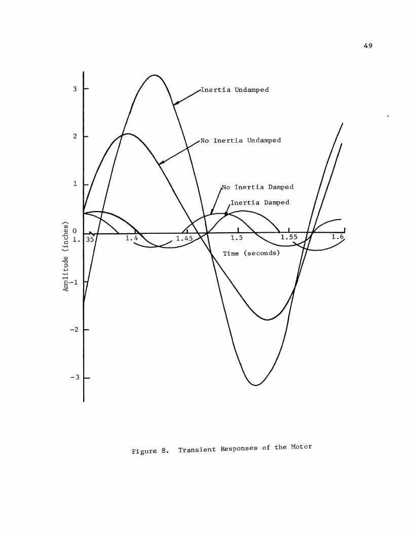
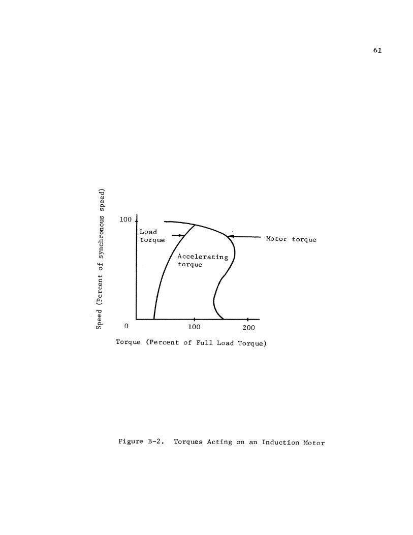
in amplitudes for various cases, graphs are plotted as follows:

1. Figure (8) - Transient responses of the motor for inertia and

no inertia damped as well as undamped cases. The time interval

was taken between 1.35 sec. to 1.6 sec., when maximum transient

amplitudes occur.

2. Figure (9) - Transient responses of the floor are plotted

for the same interval (1.35 sec. to 1.6 sec.) for inertia and

no inertia damped as well as undamped cases. The scales are

identical to those in Figure (8).

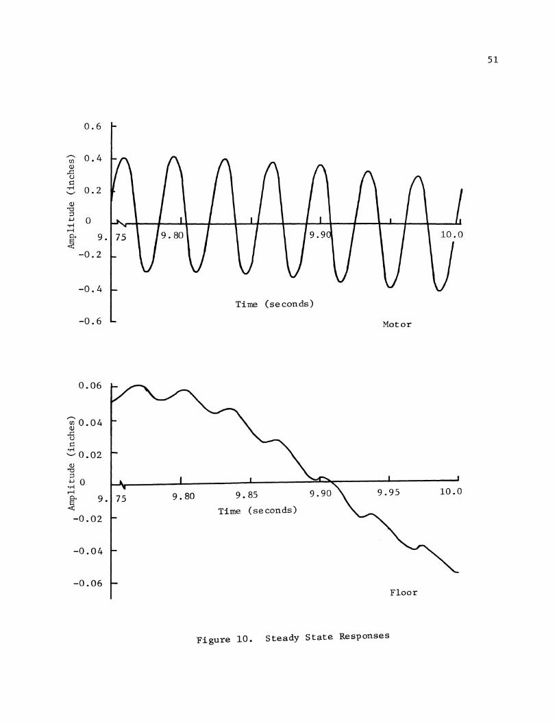
3. Figure (10) - shows the graphs of steady state responses

of motor and floor for the damped inertia case during the time

9.75 to 10.0 seconds. Note that the scales are different from

those of previous graphs. It can be seen that the response of

the floor consists of superposition of the forcing frequency

43

(29 cps) and the lower resonant frequency (2 cps) of the system.

The latter frequency is part of the transient response of the

system and will disappear eventually. However, a long time

interval is required for its elimination because the frequency

is low and no damping is present in the floor.

For a relatively large unbalanced weight (50 lbs.), an entirely

different picture is seen (see Table III). We get large differences

in the amplitudes between the inertia and no inertia, damped as

well as undamped cases. The differences between transient and steady

state amplitudes are significant even for the case without inertia

torque. For the undamped case with inertia torque, the motor never

reaches its design speed, instead, the speed fluctuates about the

second natural frequency, i.e., 29 rad./sec. This occurs because of

the large inertia torque which prevents the motor from reaching its

operating speed. The maximum transient undamped amplitude of the

motor when inertia torque is considered is 15 11 and that of floor is

about 2". For the no inertia undamped case, the amplitudes are 5"

44

and 0.54" respectively. These results indicate the pronounced effect

of inertia torque when the unbalanced mass is very large. In the

damped case when inertia torque is considered, the motor reaches 176

rad./sec. in about 14 seconds. However, this increase is not contin-

uous, because of the interaction between the inertia torque and the

accelerating torque. The force transmissibility at steady state,

when the effect of inertia torque is not considered, is about 30% larger

than that for the corresponding case where the unbalance weight is

0.25 lb. The difference in transmissibility is due to the presence of

* the transient response at 2 cps. When damping is present, this

response will disappear eventually and the force transmissibility

will decrease. Values for transmissibilities shown in Tables are

obtained from an average of peak values at 5 and 10 seconds.

C. Confirmation of Results

In order to confirm the results obtained by the Runge-Kutta

method of order four, the Continuous System Modeling Program (CSMP)

was used. This system is available at the Computer Center, University

of Missouri-Rolla, and is mainly used for solving coupled linear and

non-linear differential equations. A choice of integration scheme is

available at the option of the user. For the purpose of comparison,

Simpson's, Hammings, and Runge-Kutta method of order four were used.

The results obtained were found comparable, with difference occurring

*For all undamped cases, when inertia torque is not considered, the

force transmissibility is 0.00011, provided responses at resonant

frequencies are not included.

only after the third decimal place.

For the case when the motor is operated without any external

load and an unbalance weight of 1/2 lb., the results obtained using

the Foss method, i.e., the Convolution Integral solution, were not

comparable to the results of either the Runge-Kutta method or any

method of the CSMP. The error is suspected either in mathematics

of the Convolution Integral Solution or in the program itself. It

45

is necessary to mention here that if a procedure suitable for evalu­

ating equation (34) is developed, the Foss method will give the

correct responses of the system. (The damped natural frequencies

24.96 rad./sec. and 12.07 rad./sec. were obtained by the Foss method.)

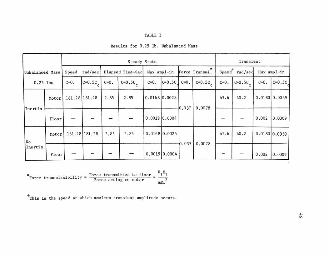
TABLE I

Results for 0.25 lb. Unbalanced Mass

Steady State

* Unbalanced Mass Speed rad/sec Elapsed Time-Sec Max ampl-in !Force Transmi. '

0.25 lbs C=O. C=0.5C C=O. C=0.5C C=O. C=0.5Cc C=O. C=0.5C c c c

Motor 181.28 181.28 2. 85 2. 85 0.0168 0.0028

Inertia 0.037 0.0078

Floor - - - - 0.0019 0.0004

Motor 181.28 181.28 2.85 2.85 0.0168 0.0025

No Inertia

u.037 0.0078

Floor - - - - 0.0019 0.0004

* Force transmissibility = Force transmitted to floor _ KlXl Force acting on motor - ----2

~

+This is the speed at which maximum transient amplitude occurs.

Transient

+ Speed rad/sec Max ampl-in

C=O. C=0.5C C=O. C=0.5C c

45.6 40.2 0.0180 0.0039

- - 0.002 0.0009

45.6 40.2 0.0180 0.0039

- - 0.002 0.0009

q

.j::o.

"'

Unbalanced Mass Speed rad/sec

30 lbs C=O. C=0.5C c

Motor 179.5 179.5

Inertia

Floor - -

Motor 181.28 181.28

No Inertia

Floor - -

TABLE II

Results for 30 lbs. Unbalanced Mass

Steady State

Elapsed Time-Sec Max ampl-in Force Transmi.

C=O. C=O. 5C C=O. C=0.5Cc C=O. C=0.5C c c

4.88 4.88 2. 70 o. 35

0.052 0.0098

- - 0.32 0.06

4.2 4.2 2.2 o. 350

0.040 0.0098

- - 0.25 0.06

Transient

Speed rad/sec Max ampl-in

C=O. C=O .5C c C=O. ~=0.5C

35.9 51.8 3.31 o. 491

- - 0.346 0.118

42.8 49.8 2.62 0. 491

- - o. 30 0.117

c

.,::­"-1

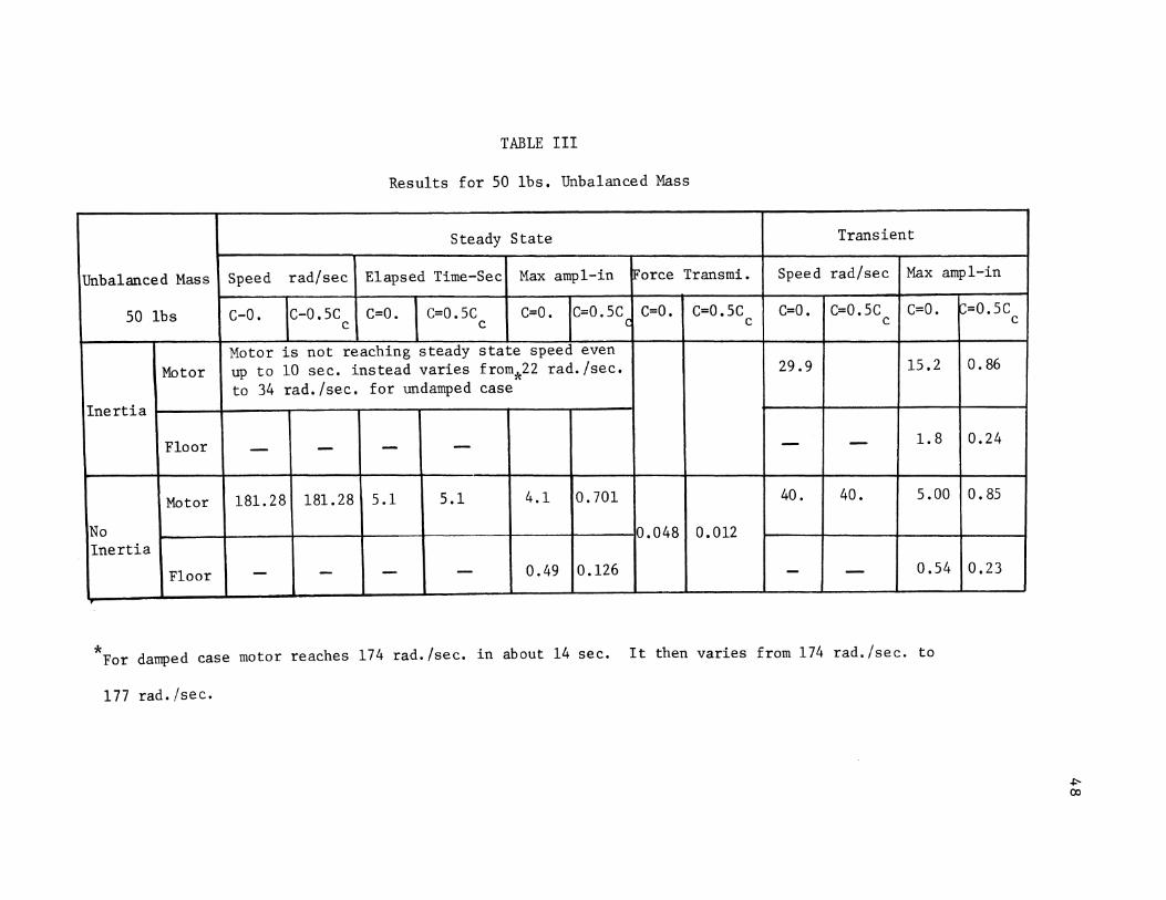
TABLE III

Results for SO lbs. Unbalanced Mass

Steady State Transient

Unbalanced Mass Speed rad/sec Elapsed Time-Sec Max ampl-in tforce Transmi. Speed rad/sec Max ampl-in

SO lbs C-0. c-o.sc C=O. C=O.SC C=O. C=O.SCc C=O. C=O.SC C=O. C=O. SC C=O. ~=0.5C c c c c

Motor is not reaching steady state speed even Motor up to 10 sec. instead varies from*22 rad./sec. 29.9 15.2 0. 86

to 34 rad./sec. for undamped case Inertia

Floor - - - - - - 1.8 0.24

Motor 181.28 181.28 5.1 S.l 4.1 0. 701 40. 40. s.oo 0. 85

No 0.048 0.012 Inertia

Floor - - - - 0.49 0.126 - - 0.54 0.23

*For damped case motor reaches 174 rad./sec. in about 14 sec. It then varies from 174 rad./sec. to

177 rad. /sec.

c

~ 00

49

3 ~nertia Undamped

2 No Inertia Undamped

1 o Inertia Damped

-2

-3

Figure 8. Transient Responses of the Motor

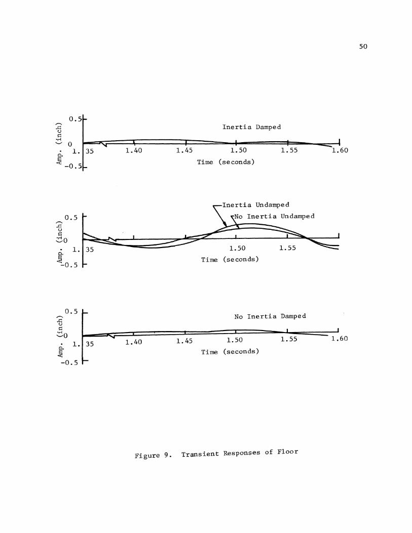
o.s ,....., 'B s::

"M .._, 0 0.. 1. 35

~ -0.5

0.5 ,....., .£::

C)

s:: .::-o P. 1.

~0.5

. 1. 35

t -0.5

1.40

1.40

Inertia Damped

1.45 1.50 1.55

Time (seconds)

Inertia Undamped

No Inertia Undamped

1.50

Time (seconds)

1.55

No Inertia Damped

1.45 1.50 1.55

Time (seconds)

Figure 9. Transient Responses of Floor

50

1.60

1.60

51

0.6

-'"""' 0.4 UJ (!)

..c t) p . ..., 0.2 '-'

(!) '"d ;::l

.j..J 0 . ..., r-1 p.. 9. ~

-0.2

-0.4

Time (seconds)

-0.6 Motor

0.06

9. 75 9. 80 9. 85 10.0

Time (seconds) -0.02

-0.04

-0.06 Floor

Figure 10. Steady State Responses

VI. CONCLUSIONS

Generally, the design of vibration isolators is based on the

steady state response of the system for the following reasons:

1. The transient period usually lasts for only a few seconds and is

followed by steady state vibration.

2. It is assumed that no annoying or potentially destructive

behavior occurs during the transient period, during which the system

accelerates to its operating speed.

However, these reasons are not always valid. As shown in

Chapter V, the system may remain in the transient condition for an

indefinite time, during which large amplitudes and forces can occur.

The following guidelines are suggested for determining whether

transient response, inertia torque, or damping should be considered

in the design or analysis of vibration isolators.

52

1. For relatively small unbalanced forces, the effect of inertia

torque can be neglected provided the system reaches its steady state

speed within a few seconds. In this case, the increases in amplitudes

during the transient period, as compared to the steady state values,

are relatively small for all values of damping.

2. When large unbalanced forces are present and the system has little

or no damping, the transient response (with inertia torque included)

must be calculated in order to obtain maximum amplitudes, forces, and

terminal speed. For example, transient analysis of the system with a

30 lbs. unbalance weight showed that the motor reaches 179 rad./sec.

53

in 4.8 sec. and then varies from 179 rad./sec. to 181 rad./sec. For

a 50 lbs. unbalance weight without damping, the motor never reaches

its steady state speed but fluctuates around its resonance frequency,

i.e., 29 rad./sec. with a maximum amplitude of 15 inches. Thus a

transient analysis may dictate the use of stops or other measures to

limit system amplitudes. Note also that failure to include the

inertia torque in this case leads to the erroneous conclusion that

the motor reaches its operating speed in 5.1 sec. with only a small

increase in maximum amplitude during the transient period. Finally,

when large unbalanced forces occur in a system having significant

damping, a transient analysis (with inertia torque included) may be

needed to determine the time required to reach terminal speed. For

example, the results for a 50 lbs. unbalance weight show that the motor

takes about 14 sec. to reach a speed of 176 rad./sec.

3. Assumption of vertical motion is justified in cases where the

system is constrained to move only in vertical direction or where

lateral and rotational stiffnesses are large. In the latter case,

however horizontal and rotational motions may have to be considered '

when vertical amplitudes become large; the case in which the unbalance

weight was 50 lbs. is an example for this.

54

VII. APPENDICES

55

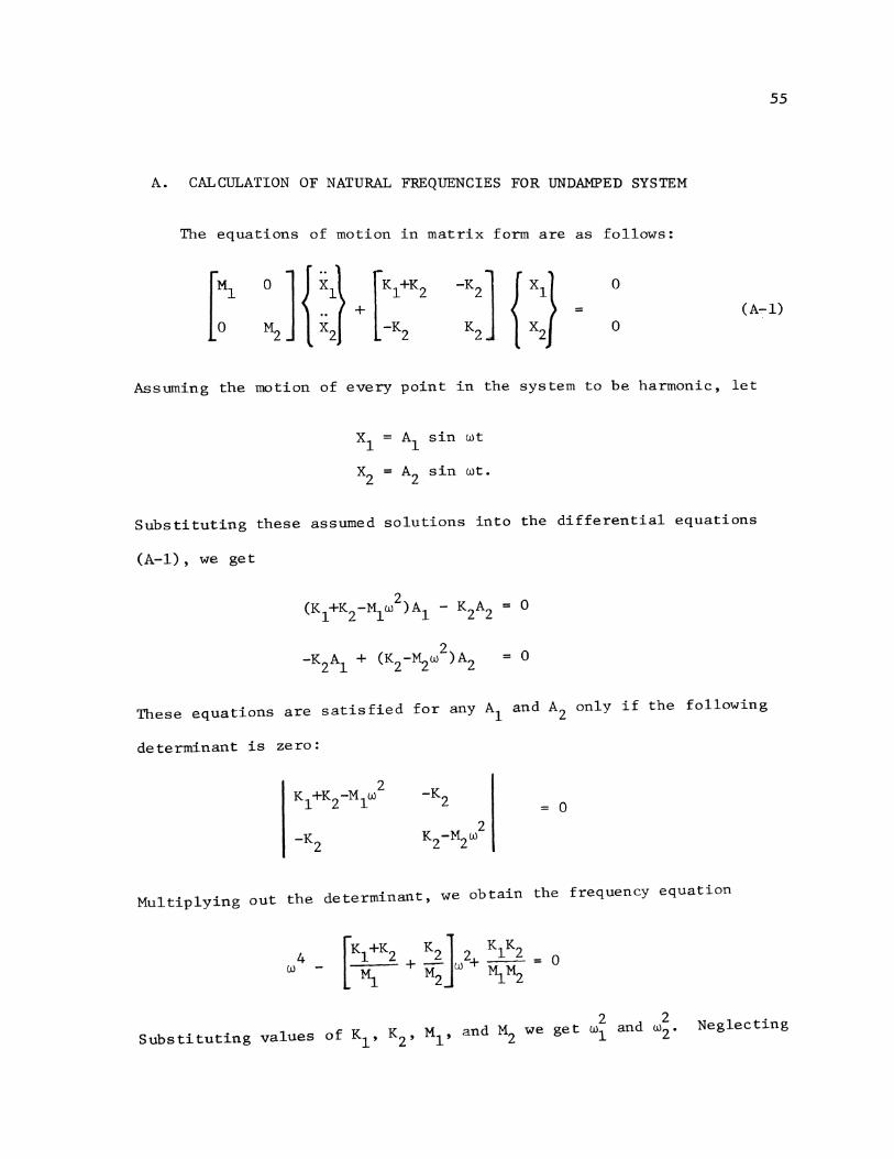
A. CALCULATION OF NATURAL FREQUENCIES FOR UNDAMPED SYSTEM

The equations of motion in matrix form are as follows:

0

= (A-1) 0

Assuming the motion of every point in the system to be harmonic, let

x1 A1 sin wt

x2 A2 sin wt.

Substituting these assumed solutions into the differential equations

(A-1), we get

0

0

These equations are satisfied for any A1 and A2 only if the following

determinant is zero:

-K 2

-K 2 0

Multiplying out the determinant, we obtain the frequency equation

4 w

2 2 Substituting values of K1 , K2 , M1 , and M2 we get w1 and w2 . Neglecting

56

negative signs as being of no physical significance, we arrive at

two natural frequencies w = 1

12.04 rad./sec. and w2 = 29.18 rad./sec.

These values agree with those obtained by the Foss Method. The

damped natural frequencies (obtained by the Foss Method) are 12.07

rad./sec. and 24.96 rad./sec.

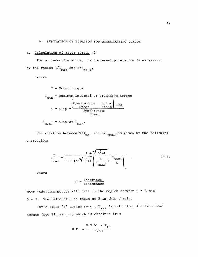
B. DERIVATION OF EQUATION FOR ACCELERATING TORQUE

a. Calculation of motor torque [5]

For an induction motor, the torque-slip relation is expressed

by the ratios T/T and S/S T' max max

where

T Motor torque

T max

Maximum internal or breakdown torque

s Slip ( Synchronous _ Rotor

S eed S eed Synchronous

Speed

S T = Slip at T . max max

100

57

The relation between T/T and S/S T is given by the following max max

expression:

where

T --= T max 1 + l/2VQ2+l(s s

maxT

Reactance Q = Resistance

+ s maxT

s

Most induction motors will fall in the region between Q

Q = 7. The value of Q is taken as 5 in this thesis.

(B-1)

3 and

For a class 'B' design motor, T is 2.15 times the full load max

torque (see Figure B-1) which is obtained from

H.P. R.P.M. x Tfl

5250

where Tfl = Full load torque.

From this relation

Tfl 3600 lb. in.

(As mentioned in Chapter V, the motor 1"s 4 pole 60 100 H p - , cps, .. ,

1750 R.P.M.)

Therefore,

T max

7740 lb. in.

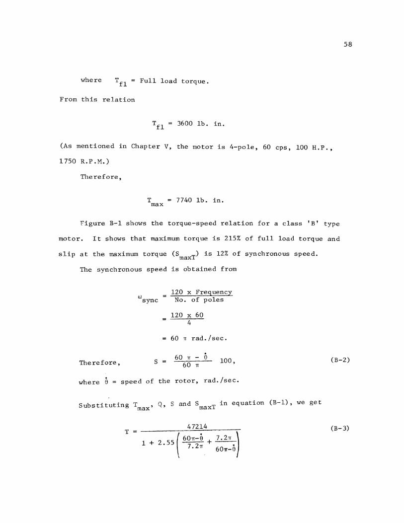
Figure B-1 shows the torque-speed relation for a class 'B' type

motor. It shows that maximum torque is 215% of full load torque and

slip at the maximum torque (S T) is 12% of synchronous speed. max

The synchronous speed is obtained from

(l) sync

120 x Frequency No. of poles

120 X 60 4

60 n rad./sec.

58

Therefore, s 6o 'IT - e 60 'IT

100, (B-2)

. where 8 speed of the rotor, rad./sec .

Substituting Tmax' Q, Sand SmaxT in equation (B-1), we get

T 47214

1 + 2 55 ( 6on-e + • 7. 2'TT

7.2'TT ) 60n-8

(B-3)

Q) ::l

B' 0

E-f

300

200

100

0 100

Speed (Percent of Synchronous Speed)

Figure B-1. Torque-Speed Curve for an Induction Motor

59

60

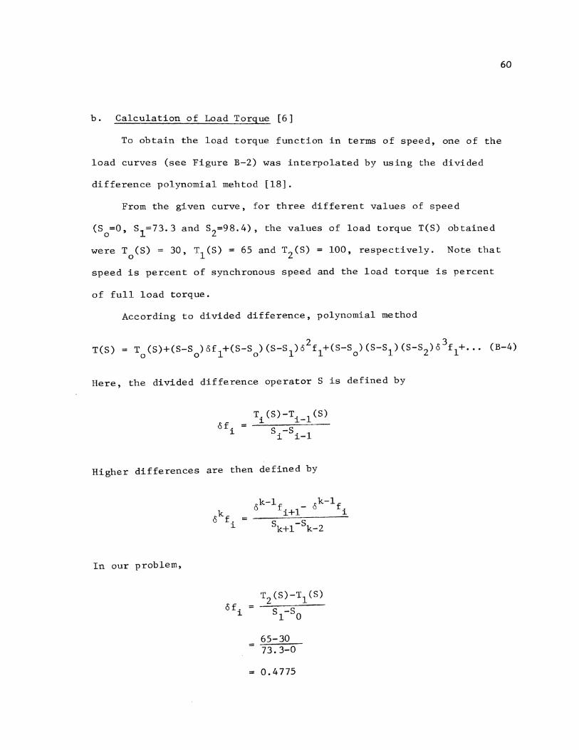
b. Calculation of Load Torque [6]

To obtain the load torque function in terms of speed, one of the

load curves (see Figure B-2) was interpolated by using the divided

difference polynomial mehtod (18].

From the given curve, for three different values of speed

(8 0 =0, 81=73.3 and 82=98.4), the values of load torque T(8) obtained

100, respectively. Note that

speed is percent of synchronous speed and the load torque is percent

of full load torque.

According to divided difference, polynomial method

T(8)

Here, the divided difference operator S is defined by

of. ]..

T. (S)-T. 1 (s) ].. ]..-

s.-8. 1 ].. ]..-

Higher differences are then defined by

k-1 k-1 0 fi+l- 0 fi

8k+l-8k-2

In our problem,

of. T2 (s)-T1 (S)

= 81-80 ]..

65-30 73.3-0

= 0. 4 775

61

100

Motor torque

0 100 200

Torque (Percent of Full Load Torque)

Figure B-2. Torques Acting on an Induction Motor

=

T2 (S)-T1 (S)

s2-sl

100-65 98.4-73.3

1. 394

= .::::;1..::.... -::-39::,..4..:...-,...;0:...;·:....;4:..:.7-=-7=-5 98.4-0

0.0093

62

Substituting all the necessary values in equation (B-3), '"e get

T(S) = 30+(S-0)0.4775+(S-0)(8-73.3)0.0093

Simplifying,

T(S) = 0.00938 2-0.20428+30.0

As mentioned earlier, T(S) is percent of full load torque and can

also be written as

T(S)

From this,

Load torque

Load torque x 100 Full load torque

Full load torgue x T(S) 100

= 3600 (0.009382-0.2042S+30.0) 100

= 0.3348S2-7.3512S+l080.0

Here the value of slip (S) is given by equation (B-2).

(B-5)

The net accelerating torque (TN) developed by the motor is then

the difference of motor torque given by (B-3) and load torque given

by (B-5). This value of TN is then used in equation (13) in

Chapter III to solve for 8(t).

63

64

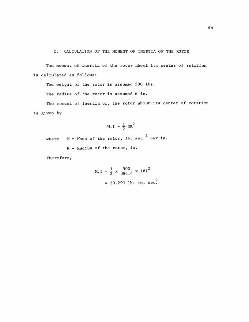
C. CALCULATION OF THE MOMENT OF INERTIA OF THE ROTOR

The moment of inertia of the rotor about its center of rotation

is calculated as follows:

The weight of the rotor is assumed 500 lbs.

The radius of the rotor is assumed 6 in.

The moment of inertia of, the rotor about its center of rotation

is given by

where M

M. I .!_ MR2 2

2 Mass of the rotor, lb. sec. per in.

R Radius of the rotor, in.

Therefore,

M. I 1 500 X ( 6 )2 2 X 386.4

= 23.291 lb. 2

in. sec.

1.

2.

3.

4.

5.

6.

7.

8.

9.

10.

11.

12.

13.

14.

15.

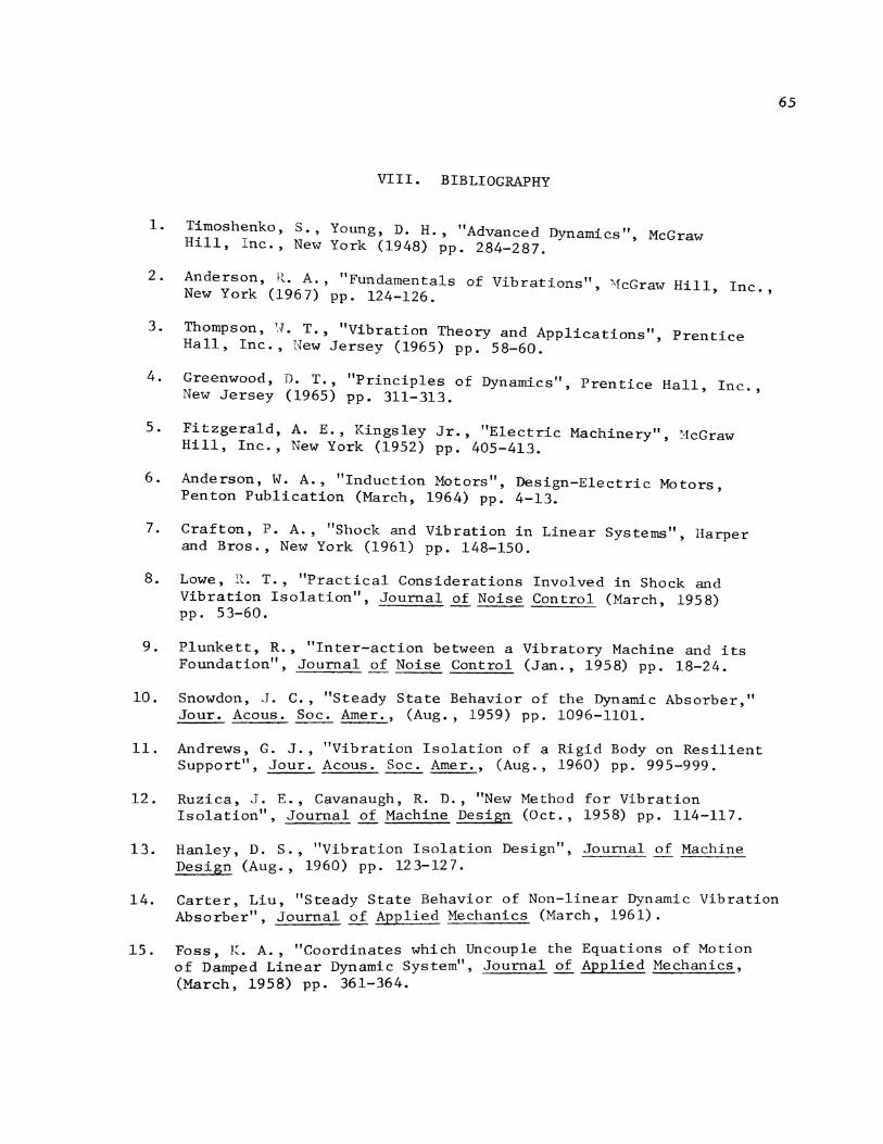
VIII. BIBLIOGRAPHY

Timoshenko, S., Young, D. H., "Advanced Dynamics", McGraw Hill, Inc., New York (1948) pp. 284-287.

Anderson, R. A., "Fundamentals of Vibrations", -:-.fcGraw Hill, Inc., New York (1967) pp. 124-126.

Thompson, '::J. T., "Vibration Theory and Applications", Prentice Hall, Inc., New Jersey (1965) pp. 58-60.

Greenwood, D. T., "Principles of Dynamics", Prentice Hall, Inc., New Jersey (1965) pp. 311-313.

Fitzgerald, A. E., Kingsley Jr., "Electric Machinery", ~1cGraw Hill, Inc., New York (1952) pp. 405-413.

Anderson, W. A., "Induction Motors", Design-Electric Motors, Penton Publication (March, 1964) pp. 4-13.

Crafton, P. A., "Shock and Vibration in Linear Systems", Harper and Bros., New York (1961) pp. 148-150.

Lowe, H .• T., "Practical Considerations Involved in Shock and Vibration Isolation", Journal of Noise Control (March, 1958) pp. 53-60.

Plunkett, R., "Inter-action between a Vibratory Machine and its Foundation", Journal of Noise Control (Jan., 1958) pp. 18-24.

Snowdon, J. C., "Steady State Behavior of the Dynamic Absorber," Jour. Acous. Soc. Amer., (Aug., 1959) pp. 1096-1101.

Andrews, G. J. , "Vibration Isolation of a Rigid Body on Resilient Support", Jour. Acous. Soc. Amer., (Aug., 1960) pp. 995-999.

Ruzica, J. E., Cavanaugh, R. D., "New Method for Vibration Isolation", Journal of Machine Design (Oct., 1958) pp. 114-117.

Hanley, D. S., "Vibration Isolation Design", Journal of Machine Design (Aug., 1960) pp. 123-127.

Carter, Liu, "Steady State Behavior of Non-linear Dynamic Vibration Absorber", Journal of Applied Mechanics (March, 1961).

Foss K. A., "Coordinates which Uncouple the Equations of Motion of D~mped Linear Dynamic System", Journal of Applied Mechanics, (March, 1958) pp. 361-364.

65

16. Patel, B. B., "A Computerized Method for Finding the Dynamic Response of Multi-Mass Systems with Damping to Arbitrary Inputs", Thesis, University of Missouri-Rolla.

17. Buxton, V. S., "Driven-Machine Mechanics", Journal of Machine Design Design-Electric Motors, Penton Publication (March, 1964) pp. 24-29.

18. Conte, S. D., "Introduction to Numerical Analysis and Digital Computers", McGraw Hill, Inc., New York (1965) pp. 88-96.

19. Supplementary Report, Department of Mechanical and Aerospace Engineering, University of Missouri-Rolla.

20. Caughey, T. K., "Classical Normal Modes in Damped Linear Dynamic Systems", .Journal of Applied Mechanics, pp. 269-271.

66

67

IX. VITA

Hemendra Shantilal Acharya was born on October 21, 1943, at

Halvad, Gujarat State, India. He graduated from C.V.O.S. High

School, Bombay, India in 1960. He received a B.S. in Mechanical

Engineering from the Gujarat University, Ahmedabad, India in 1965.

Immediately thereafter he was employed by Mukand Iron and

Steel Works Limited, Bombay, in the Maintenance and Development

Department.

In January 1969, he enrolled in the University of Missouri-

Rolla for work toward his Master's Degree in Mechanical Engineering.