Transient Queueing Analysis - William & Maryleemis/2012informsjocb.pdfThe trafﬁc intensity of the system is ’D‰=s„. The system consists of a single queue with customers waiting

INFORMS Journal on ComputingVol. 24, No. 1, Winter 2012, pp. 10–28ISSN 1091-9856 (print) � ISSN 1526-5528 (online) http://dx.doi.org/10.1287/ijoc.1110.0452

© 2012 INFORMS

Transient Queueing Analysis

William H. KaczynskiDepartment of Mathematical Sciences, United States Military Academy, West Point,

New York 10996, [email protected]

Lawrence M. Leemis, John H. DrewDepartment of Mathematics, College of William & Mary, Williamsburg, Virginia 23187

{[email protected], [email protected]}

The exact distribution of the nth customer’s sojourn time in an M/M/s queue with k customers initiallypresent is derived. Algorithms for computing the covariance between sojourn times for an M/M/1 queue

with k customers present at time 0 are also developed. Maple computer code is developed for practical appli-cation of transient queue analysis for many system measures of performance without regard to traffic intensity(i.e., the system may be unstable with traffic intensity greater than 1).

Key words : exponential distribution; Poisson process; queueing theoryHistory : Accepted by Winfried Grassmann, Area Editor for Computational Probability and Analysis; received

October 2009; revised May 2010; accepted January 2011. Published online in Articles in Advance June 17, 2011.

1. IntroductionMany traditional simulation studies analyze queueingsystems in steady state, requiring appropriate warm-up periods and associated long simulation runs. How-ever, in many cases, the system being modeled neverreaches steady state; thus steady-state simulationresults do not accurately portray the system behavior.The ability to analyze transient results associated withsuch models is often complicated by intractable the-ory, leaving simulation as the only method for anal-ysis. Further complicating the transient analysis isthe effect of initial conditions (Kelton and Law 1985).Because steady-state results depend on running thesystem long enough to negate the impact of initialconditions, these steady-state results reveal nothingabout the transient behavior of the queueing system.Our purpose here is to combine new and existingresults in transient queueing analysis with a symbolicengine in computational probability.

There are many classes of queueing systems inwhich a transient analysis is required; e.g., ser-vice businesses often model queues that never reachequilibrium. The need to develop theory for tran-sient results, as opposed to steady-state results, hasresulted in wide literature in this area. Initial work intransient analysis ironically appeared as an attemptto measure when a system achieved equilibrium.Law (1975) notes the consequences of failing to ade-quately account for the initial transient period, whichled Gafarian et al. (1976) to develop a comprehen-sive framework for the initial transient problem.Morisaku (1976) addresses the time to equilibrium

in simulations modeling the M/M/1 queue and pro-vides schematics for the transition probabilities givenk ≥ 0 customers initially present at time t = 0. Grass-mann (1977) compares three methods for findingtransient solutions in Markovian queueing systems—Runge–Kutta, Liou’s method, and randomization—where randomization is shown as superior for largesparse transition matrices. Pegden and Rosenshine(1982) provide a closed-form expression for the prob-ability of exactly i arrivals and j servicings overa time horizon of length t in an M/M/1 queuestarting empty and idle; this expression allows thecalculation of certain performance measures for aspecified time period. Odoni and Roth (1983) takean empirical approach to compare observed and pre-dicted transient-state queue lengths for the M/M/1queue, noting that for small values of t, the expectedqueue length is strongly influenced by initial con-ditions, and they provide a good approximation foran upper bound of the time to steady state. Keltonand Law (1985) consider the M/M/s 4s ≥ 15 queueand provide expressions to calculate the probabili-ties of having up to n + k customers in the systemupon the arrival of the nth customer, where k is thenumber of customers in the system at time t = 0.Kelton and Law then apply these calculations to avariety of measures of performance with implicationsto convergence on steady-state delays, and they offermethods for choosing queue initialization in simula-tion. Much of the work in this paper is motivatedby their results. Kelton (1985) extends the previouswork by considering M/Em/1 and Em/M/1 queues.Parthasarathy (1987) provides a transient solution for

10

INFORMS

holds

copyrightto

this

article

and

distrib

uted

this

copy

asa

courtesy

tothe

author(s).

Add

ition

alinform

ation,

includ

ingrig

htsan

dpe

rmission

policies,

isav

ailableat

http://journa

ls.in

form

s.org/.

Kaczynski, Leemis, and Drew: Transient Queueing AnalysisINFORMS Journal on Computing 24(1), pp. 10–28, © 2012 INFORMS 11

the probability that there are n customers in the sys-tem at time t for an M/M/1 queue. Abate and Whitt(1988) use Laplace transformations to analyze sometransient results of interest in the M/M/1 queue.Leguesdron et al. (1993) provide transient probabili-ties for the M/M/1 queue by inverting the generatingfunction of the uniformized Markov chain describingthe M/M/1 process. Transient distributions of cumu-lative reward are calculated by de Souza e Silva et al.(1995) using uniformization, where the distributionof cumulative reward is over a finite interval withreward rates represented by Markov model states.Grassmann (2008) investigates warm-up periods insimulation and shows that in many cases these warm-up periods should not be used, especially if the simu-lation begins in a high probability state. In this paperwe focus on the transient analysis of the M/M/1and the more general M/M/s queues—specifically, onthe distribution of the nth customer’s sojourn time,which is the sum of the nth customer’s delay andservice times. Almost all the above-mentioned refer-ences address measures of performance specified overa finite time interval and are the results of numer-ical work. This is in stark contrast to the measuresproposed here, which are based on the exact distribu-tion of specific customers. Rather than arriving at theresults numerically, a computer algebra system is uti-lized that offers exact measures of performance basedon a given number of customers.

The M/M/s queue is defined in §2 for a positiveinteger s, and a method is given for calculating theprobability distribution of the number of customersan arriving customer sees upon arrival to an M/M/squeue. Section 3 describes how the sojourn time dis-tribution is calculated for a given customer in anM/M/s queue with k ≥ 0 customers initially presentin the system. Section 4 includes examples using theimplemented procedures to calculate exact sojourntime distributions, related measures of performance,and graphical illustrations for varying parameterssuch as traffic intensity and number of customersin the system. Section 5 offers two approaches forcalculating the covariance and correlation amongcustomers in an M/M/1 queue. Sections 6 and 7extend the covariance and correlation calculations byautomating the process of finding the joint probabil-ity density function of two sojourn times, and pro-vide the exact covariance and correlation calculationsfor varying traffic intensities and account for occa-sions where customers are present at time 0. Section 8concludes the paper with a review of the contentand offers areas of further study. Commented code isavailable for all computations conducted here.

2. Basics of the M/M/s QueueThe M/M/s queue is governed by independent andidentically distributed (iid) exponential interarrival

times (the arrival stream is a Poisson process) witharrival rate � and iid exponential service times amongs identical servers, each with service rate �. The inter-arrival times and the service times are mutually inde-pendent. The traffic intensity of the system is �= �/s�.The system consists of a single queue with customerswaiting to be serviced by one of the s identical parallelservers. If an arriving customer finds at least one idleserver, the customer immediately proceeds to service;otherwise, the customer joins the single queue of thosewaiting for service in a first-come, first-served manner.To achieve classic steady-state results, the traffic inten-sity must satisfy � < 1. This critical assumption is notrequired in transient analysis described here, becausethe system of interest never reaches equilibrium.

Let Pk4n1 i5 be the probability that, upon the arrivalof the nth customer, there are i customers in the sys-tem including the nth customer (in queue or in ser-vice) given k customers are present at time t = 0.Using propositions provided by Kelton and Law(1985), reprinted here for completeness (proofs areavailable in the reference) as well as a recursion algo-rithm, Pk4n1 i5 for i = 1121 0 0 0 1n+ k can be computed.Using these probabilities, it is possible to find the dis-tribution of the sojourn time for the nth customer inan M/M/s queue given k customers are present attime t = 0. Proposition 1 addresses the case of no exitsprior to the nth customer’s arrival given k ≥ 1. Propo-sition 2 is identical to Proposition 1 except that thesystem is empty and idle at t = 0 (i.e., k = 0). Proposi-tion 3 addresses the case that the first customer findsi− 1 other customers present for k > 0. Proposition 4is the more general case that customer n ≥ 2 finds iother customers present given k ≥ 0.

Proposition 1. If k ≥ 1, then for n≥ 1,

Pk4n1k+n5=

6�/4�+ 157n if k ≥ s1

�n/

n∏

j=1

6�+ 4k+ j − 15/s7 if k+n≤ s1

�n/

[

4�+ 15n−s+ks−k∏

j=1

6�+ 4k+ j − 15/s7]

if k < s < k+n0

Proposition 2. For n≥ 1,

P04n1n5=

�n/

n∏

j=1

6�+4j−15/s7 if n≤s1

�n/

[

4�+15n−ss∏

j=1

6�+4j−15/s7]

if n>s0

INFORMS

holds

copyrightto

this

article

and

distrib

uted

this

copy

asa

courtesy

tothe

author(s).

Add

ition

alinform

ation,

includ

ingrig

htsan

dpe

rmission

policies,

isav

ailableat

http://journa

ls.in

form

s.org/.

Kaczynski, Leemis, and Drew: Transient Queueing Analysis12 INFORMS Journal on Computing 24(1), pp. 10–28, © 2012 INFORMS

Proposition 3. If k ≥ 1, then for 2 ≤ i ≤ k,

Pk411i5

=

8�/6�+4i−15/s79

·

k−i+1∏

j=1

81−�/6�+4k−j+15/s79 if k≤s1

�/4�+15k−i+2 if k>s and i>s1

8�/64�+15k−s+16�+4i−15/s779

·

s−i∏

j=1

81−�/6�+4s−j5/s79 if i≤s<k0

Proposition 4. For n≥ 2, and 2 ≤ i ≤ k+n− 1,

Pk4n1i5=

6�/4�+157k+n−1∑

j=i−1

61/4�+157j−i+1Pk4n−11j5

if i>s1

8�/6�+4i−15/s79

·

{ s−1∑

j=i−1

[j−i+1∏

h=1

81−�/6�+4j−h+15/s79]

·Pk4n−11j5+[ s−i∏

h=1

81−�/6�+4s−h5/s79

]

·

k+n−1∑

j=s

61/4�+157j−s+1Pk4n−11j5}

if i≤s0

Using these four propositions, Pk4n115 is calculatedby subtracting the complementary probability fromone. These results can be generated by invoking theMaple procedure MMsQprob(n,k,s), where

• n is the index of the customer of interest,• k is the number of customers in the system at

time t = 0, and• s is the number of identical parallel servers.

The procedure is written in Maple and uses A Prob-ability Programming Language (APPL), which canbe downloaded for free at http://www.APPLsoftware.com and is described in Glen et al. (2001). Wechoose to calculate the distribution of the sojourn timebecause it is a purely continuous random variable thatenables us to exploit associated procedures in APPL.

3. Creating the Sojourn TimeDistribution

Once the necessary Pk4n1 i5, i = 1121 0 0 0 1n + k, prob-abilities are calculated, the exact sojourn time distri-bution for the nth customer can be calculated. Wedefine Xn as the number of customers, including cus-tomer n, in the system upon the arrival of the nthcustomer. The possible values of Xn can vary from aminimum of 1, which occurs when customer n arrives

to an empty queue with idle servers, to a maximumof n + k, which occurs when zero exits occur priorto customer n’s arrival, matching the possible val-ues for i in the expression for Pk4n1 i5. The mathe-matical derivations for both the M/M/1 and M/M/squeues make extensive use of the memoryless prop-erty, which permits the construction of the distribu-tion of Tn (the sojourn time of customer n). We presenteach case separately.

3.1. Distribution of Tn for the M/M/1 QueueFor an M/M/1 queue starting empty and idle, thedelay time of the first customer is zero because thecustomer proceeds directly to service upon arrival.Therefore, the first customer has an exponential(�)sojourn time distribution. Conditioning on cus-tomer 1’s service time, one can calculate the probabili-ties of customer 2 arriving before and after customer 1finishes service. These well-known results (Kleinrock1975, Hillier and Lieberman 2005, Winston 2004) are

Pr4Y <X5=�

�+�1 Pr4X < Y 5=

�

�+�1

where X is an exponential(�) interarrival time and Yis an exponential(�) service time. The first probabilityrepresents customer 2 proceeding directly to service,in which case his sojourn time is simply his servicetime (exponential(�)). The second probability repre-sents the likelihood that customer 2 will delay priorto service. Using the memoryless property, customer 2delays an exponential(�) time before being servicedin an additional exponential(�) time. Using these twoprobabilities, it is easy to see that customer 2’s sojourntime distribution is a mixture where the mix probabil-ities are P04n1 i5 and the distributions are determinedby the orderings of delays and services potentiallyencountered. It is well known that for X11X21 0 0 0 1Xn

iid exponential(�) random variablesn∑

i=1

Xi ∼ Erlang4�1n50 (1)

Using this result, the M/M/1 queue sojourn time dis-tribution for k = 0 initial customers generalizes veryelegantly to include k > 0, as indicated in Table 1.Line i of Table 1, where i = 1121 0 0 0 1n+k, occurs withprobability Pk4n1 i5 and lists the distribution of thesojourn time for the nth customer, conditioned on icustomers being in the system upon his arrival.

Let gi4t5 be the probability density function (PDF)of an Erlang4�1 i5 random variable. Using the condi-tional sojourn time distributions for i = 1121 0 0 0 1n+ kpotential customers in the system, each with proba-bility Pk4n1 i5, the PDF for the nth customer’s sojourntime Tn is the mixture

fn4t5=

n+k∑

i=1

Pk4n1 i5gi4t51 t > 00 (2)

INFORMS

holds

copyrightto

this

article

and

distrib

uted

this

copy

asa

courtesy

tothe

author(s).

Add

ition

alinform

ation,

includ

ingrig

htsan

dpe

rmission

policies,

isav

ailableat

http://journa

ls.in

form

s.org/.


Table 1 Conditional Sojourn Time Distributions for the M/M/1 Queue

Conditional sojournXn Delay Service time distribution

1 0 exponential(�) exponential(�)2 exponential4�5 exponential(�) Erlang4�1253 Erlang4�125 exponential(�) Erlang4�1354 Erlang4�135 exponential(�) Erlang4�145000

000

000

000

n+ k Erlang(�1n+ k − 1) exponential(�) Erlang(�1n+ k)

This result is simple in the M/M/1 case because wecan take advantage of (1), which results in a mixtureof n+ k Erlang distributions.

3.2. Distribution of Tn for the M/M/s QueueGiven s > 1 parallel identical servers, the nth cus-tomer’s sojourn time distribution is still a mixture ofn+k conditional sojourn time distributions. However,each distribution might be more complicated. Forillustration, consider an M/M/3 queue starting emptyand idle with exponential(�) arrivals and three iden-tical exponential(�) servers. It is clear that for cus-tomers 1, 2, and 3, the sojourn time is exponential(�)because all three customers proceed directly to ser-vice. Therefore, in the general case, for the number ofcustomers in the system including customer n (whichwe defined as Xn), the conditional sojourn timedistribution is exponential(�) when Xn ≤ s. How-ever, if Xn > s, then the nth customer experiences adelay while observing Xn − s service completions.When s > 1 and Xn > s, the service time distributionobserved by customers in the queue is exponentialwith a rate of s�. Using this result, it is apparent thatthe delay time for the nth customer is the sum ofXn−s independent exponential(s�) random variables,and using (1) is Erlang(s�1Xn−s). To calculate the nthcustomer’s sojourn time for a particular value of Xn,we sum his delay and service times. Table 2 shows thedistributions conditioned on the number of customersXn encountered by customer n (including himself) forthe M/M/3 queue, given k = 0 customers present at

Table 2 Conditional Sojourn Time Distributions for the M/M/3 Queuewith k = 0

Conditional sojournXn Delay Service time distribution

1 0 exponential(�) exponential(�)2 0 exponential(�) exponential(�)3 0 exponential(�) exponential(�)4 exponential(3�) exponential(�) exponential(3�)⊕ exponential(�)5 Erlang(3�, 2) exponential(�) Erlang(3�, 2)⊕ exponential(�)000

000

000

000

n Erlang(3�1n− 3) exponential(�) Erlang(3�1n− 3)⊕ exponential(�)

time t = 0. The APPL procedure Convolution calcu-lates the distribution of a sum of independent randomvariables. We use the symbol ⊕ to denote convolution.

Since Xn represents the number of customers in thesystem upon arrival of the nth customer (includinghimself), the first row in Table 2 corresponds tocustomer n arriving to an empty system, and the lastrow corresponds to no service completions prior tocustomer n’s arrival. The general form for the M/M/ssojourn time PDF is identical to (2); however, in theM/M/s case, each gi4t5 can potentially require anadditional step to calculate the distribution of a sumof random variables.

4. Transient Analysis ApplicationsIt is apparent that calculating (2) for large n is tedious.Kelton and Law (1985) acknowledge the computa-tional difficulty in achieving the Pk4n1 i5 probabilitiesalone. Conducting the added steps of up to n − sconvolutions for the M/M/s queue and then mixingthe resulting conditional distributions with the appro-priate probabilities can be complicated to implement.APPL provides the underlying computational engineto achieve exact results for such problems. The APPLprocedure Queue(X,Y,n,k,s) returns the exact sojourntime distribution for customer n. Queue subsequentlycalls MMsQprob(n,k,s), which uses recursion to calcu-late the necessary Pk4n1 i5 probabilities. APPL is capa-ble of symbolic results, as illustrated in Examples 1and 2.

Example 1. Consider an M/M/1 queue with anarrival rate � and a service rate � starting empty andidle at time t = 0. For the fourth customer, calculatethe probabilities P0441 i5 for i = 1121314.

The APPL command MMsQprob(4,0,1) returns theexact symbolic probabilities

P044115 =5�2 + 4�+ 14�+ 155

1

P044125 =�45�2 + 4�+ 15

4�+ 1551

P044135 =�243�+ 154�+ 154

1

P044145 =�3

4�+ 1531

where �= �/�. It is easy to verify that for any � > 0,∑4

i=1 P0441 i5= 1, as is required. For example, a simplesubstitution, letting �= 9/10, yields

P044115=865000

24760991 P044125=778500

24760991

P044135=299701303211 P044145=

7296859 0

Example 2. For the queue described in Example 1,calculate the fourth customer’s sojourn time distribu-tion, mean sojourn time, and sojourn time variance.

INFORMS

holds

copyrightto

this

article

and

distrib

uted

this

copy

asa

courtesy

tothe

author(s).

Add

ition

alinform

ation,

includ

ingrig

htsan

dpe

rmission

policies,

isav

ailableat

http://journa

ls.in

form

s.org/.


The APPL statementsX := ExponentialRV(lambda);Y := ExponentialRV(mu);T := Queue(X,Y,4,0,1);Mean(T);Variance(T);

calculate the desired results. The first two linesdefine the interarrival and service time distributions,and the third line calculates the fourth customer’ssojourn time distribution. The last two lines are self-explanatory. The resulting PDF is

f44t5 =1

64�+�55�4e−�t

· 430�2+ 30�3t + 24��+ 24�2�t + 6�2

+ 6�2�t

+ 9t2�4+ 12t2�3�+ 3t2�2�2

+ t3�5

+ 2t3�4�+ t3�3�251 t > 00

Using f44t5, the Mean and Variance commands return

E6T47=�5 + 6��4 + 26�2�3 + 16�3�2 + 17��4 + 4�5

�4�+�55

and

Var6T47 = 4181�2�8+ 484�3�7

+ 816�4�6+ 868�5�5

+ 574�6�4+ 244�7�3

+ 40��9+ 68�8�2

+ 12�9�+�10+ 4�105/4�24�+�51050

Substituting � = 1 and � = 10/9, for example, theresults simplify to

f44t5=5000

66854673e−10/9t

· 4361t3+ 2109t2

+ 5190t + 519051 t > 01

E6T47=2332334712380495 ≈ 1088391 and

Var6T47=383506725720906153276656445025 ≈ 2050210

The CPU time associated with the examplesis negligible. Examples 1 and 2 represent simpleapplications of these procedures that circumvent timeintensive hand calculations.

Example 3. Calculate the mean sojourn time of the30th customer in an M/M/2 queue with an arrivalrate �= 1, a service rate �= 9/20 (�= 10/9), and k = 3customers initially present.

The mean can be calculated in a single APPL state-ment by embedding the function calls:Mean(Queue(ExponentialRV(1),ExponentialRV(9/20),

30,3,2));which yields

42074703020765530930928383247885331056322365205

26343624731399405569875101728767946601484880

1386412835644747949355488763405

· 421534046672820071947860003352210296689224691

678842510431455073374994143953948660661783359

7075878645126387716456920630535−11

or, to four digits, 9.6345.

The ability to represent the sojourn time distribu-tion for the nth customer in closed form also pro-vides valuable information on asymptotic behavior forqueueing systems, including steady-state convergencerates for different initial conditions. Figure 1 showsthe mean sojourn time for customer n = 1121 0 0 0 1120in an M/M/1 queue with � = 1, � = 10/9, and� = 9/10 for several values of k. The points that areplotted have been connected by lines. As expected,despite the initial condition, all cases appear to movetoward the steady-state value of 9 with increasing n.The horizontal axis is only limited to n = 120 fordisplay purposes, and in fact, identical computationswere carried out for n > 300 customers to verify con-vergence. However, as shown in the cases where k = 6and k = 10, the convergence to steady state is notalways monotone. Additionally, in testing varioustraffic intensities, the rate of convergence to steadystate increases rapidly with decreasing traffic intensityfor varying values of k.

APPL also has the ability to calculate the closed-form cumulative distribution function (CDF) forthe nth customer’s sojourn time, which permits CDFcomparisons for varying n as well as distributionpercentiles for a given customer. The procedure callCDF(T) returns the exact CDF for customer 4 (fromExample 1). Figure 2 displays the sojourn time CDFfor varying n with fixed k = 0 and �= 9/10. The dif-ferences in CDFs across n correspond to the increasingmean attributed to the delays experienced by succes-sive customers; e.g., customer 2 has delay time 0 orexponential(�), whereas the nth customer (for n> 2)faces a finite mixture of n potential delay distribu-tions. The CDF associated with n = � corresponds

120n

10080604020

2

4

6

8 k = 10

k = 6

k = 3

k = 1

E[T

n]

0

Figure 1 M/M/1 Mean Sojourn Time for �= 9/10 Given k at t = 0

INFORMS

holds

copyrightto

this

article

and

distrib

uted

this

copy

asa

courtesy

tothe

author(s).

Add

ition

alinform

ation,

includ

ingrig

htsan

dpe

rmission

policies,

isav

ailableat

http://journa

ls.in

form

s.org/.


10t

1550

0.0

0.2

0.4

0.6

0.8

1.0

n = 2

n =7

n = 20

n = ∞F(t

)

Figure 2 M/M/1 Sojourn Time CDFs for Various n Given � = 1,�= 10/9, �= 9/10, and k = 0

to the steady-state distribution of the sojourn time,which is exponentially distributed with a mean of 9(Kleinrock 1975).

Varying k for an M/M/1 queue also providesanother basis for comparison of CDFs. Figure 3fixes n = 2 and � = 9/10, and it plots the result-ing CDFs across k. Kelton and Law (1985) make asimilar comparison using convergence to steady-statedelay time. Using the CDF for multiple values of kallows direct comparison of sojourn time percentilesfor customer n. As depicted, the sojourn time CDFfor customer 2 is extremely sensitive to the initialcondition k. As an illustration, the 80th percentiles fork = 013, and 6 are

F −12 400805≈

10935 k = 0140432 k = 3170510 k = 60

These percentiles are achieved using the APPLstatements

108t

6420

0.0

0.2

0.4

0.6

0.8

1.0

k = 0

k = 3

k = 6

F(t

)

Figure 3 M/M/1 Sojourn Time CDFs for Customer n = 2 for Various kGiven �= 1, �= 10/9, and �= 9/10

X := ExponentialRV(1);Y := ExponentialRV(10/9);Z := Queue(X,Y,2,k,1);IDF(Z,0.8);

when k = 013, and 6. The last statement, IDF(Z,0.8),numerically solves FZ4z5= 0080 on the interval 401�5.

Given the complete specification of the sojourntime distribution, one can use APPL to calculate notonly the mean but also the second, third, and fourthmoments for customer n. This is especially valuablefor steady-state analysis. It is common in simulationto verify attainment of steady-state behavior by exam-ining the mean delay or mean sojourn time. Althoughsome literature exists on estimating transient meanand variance, we are not aware of any literatureaddressing higher moments. Literature addressing thesecond moment seems mostly focused on varianceestimation and not necessarily convergence. There-fore, even when the first moment might acceptablyapproximate the steady-state value, there is reasonfor further analysis of higher moments. For exam-ple, Figure 4 displays the first four moments of thesojourn time for customer n in an M/M/1 queue,where � = 1, � = 2, and � = 1/2, with the initial con-dition k = 01418.

The code used to calculate the values plotted in Fig-ure 4 isX := ExponentialRV(1);Y := ExponentialRV(2);for i from 2 to 60 by 1 doT := Queue(X,Y,i,k,1):print(i,evalf(Mean(T)), evalf(Variance(T)),

evalf(Skewness(T)), evalf(Kurtosis(T))):od:

for k = 014, and 8. The vertical dashed lines givethe smallest customer number for which all threetransient values are within 1% of the steady-statevalue. The relatively low traffic intensity �= 1/2 wasselected purposely to allow quick convergence andeasy visual inspection. Even with this somewhat lowtraffic intensity, it is apparent that the higher momentsconverge more slowly than the lower moments. Inother scenarios where � > 1/2, the higher momentsexhibit an even slower convergence. Each verticaldashed line in Figure 4 was triggered by the k = 8curve, which suggests that the moments are more sen-sitive to a heavily preloaded system. For the casesk = 014, and 8, the customer numbers for which thetransient results were within 1% of the steady-statevalues are listed in Table 3. To verify the initial con-dition effect on the convergence rate of the first fourmoments, k was increasingly incremented beyond 8and displayed a further slowing of convergence.

INFORMS

holds

copyrightto

this

article

and

distrib

uted

this

copy

asa

courtesy

tothe

author(s).

Add

ition

alinform

ation,

includ

ingrig

htsan

dpe

rmission

policies,

isav

ailableat

http://journa

ls.in

form

s.org/.


0

4

6

8

10

12

2.5

2.0

1.5

1.0

0.5

2.0

1.5

1.0

0.5

4

3

2

1

0

10 20 30 40 50 60

n

n = 56

n = 50

n = 46

n = 36

k = 8

k = 8

k = 8

k = 8

k = 4

k = 4

k = 4

k = 4

k = 0

k = 0

k = 0

k = 0

E[(

(Tn

–�

)/�

)4 ]E

[((T

n–�

)/�

)3 ]E

[Tn]

Var

[Tn]

n

n

n

Figure 4 First Four Moments of the M/M/1 Sojourn Time forCustomers 2–60 for �= 1/2 and k = 01418 (the Arrival RateIs �= 1 and the Service Rate Is �= 2, Resulting in Steady-State Values for the Four Measures of Performance of 11112and 9)

5. Covariance and Correlation in theM/M/1 Queue

The dependence exhibited in sojourn times of suc-cessive customers is one reason for the difficulty incalculating interval estimators for queue measures ofperformance. In the simplest case, consider an ini-tially empty and idle M/M/1 queue with interarrivaland service rates � and �, respectively. Our desire isto calculate the covariance between the sojourn timesof customers 1 and 2. We outline two approaches to

Table 3 Smallest Customer Number Where theSojourn Time Transient Result Is Within 1%of Steady State for an M/M/1 Queue withk = 01418 and �= 1/2

k = 0 k = 4 k = 8

E6T 7 19 21 36√

Var6T 7 27 29 46

E644T −�5/� 537 28 29 50

E644T −�5/� 547 34 35 56

modeling the events in the queue that will be helpfulin the presentation of the analytic result.

5.1. Discrete-Event Simulation ApproachesAs previously discussed, customer 1 proceeds directlyto service, and two cases exist for customer 2. In thefirst case, customer 2 proceeds directly to service. Inthe second case, he delays proceeding to service untilcustomer 1’s departure. Both cases are shown in Fig-ure 5. This section introduces two approaches for gen-erating the first two customers’ sojourn times.

The first approach is a standard discrete-event sim-ulation model. Without loss of generality, assumethat customer 1 arrives at time 0. In the next-eventapproach, customer 1’s service time is distributedaccording to the exponential(�) service time distribu-tion. The arrival time a2 for customer 2 is distributedaccording to the exponential(�) time-between-arrivalsdistribution. If the arrival occurs after customer 1’sservice completion (case 1), then customer 2 also hasan independent exponential(�) service time, whichin this case is equal to his sojourn time T2. In thesecond case where customer 2’s arrival time occursbefore customer 1’s completion of service (a2 < T1),customer 2 delays for T1 − a2 time units. We then addthe exponential(�) service time to the delay time tocalculate T2.

We define the gap that occurs in case 2 as Y = T1 −

a2. It can be shown analytically that Y ∼ exponen-tial(�) by computing the distribution of the differenceT1 −A2, where A2 is the random arrival time of the sec-ond customer and is distributed exponential(�), andthen truncating the result on the left at zero. (Alter-natively, it can be reasoned that Y ∼ exponential(�)by the memoryless property for the exponential dis-tribution because the remaining service time for cus-tomer 1 after customer 2’s arrival has the samedistribution as an unconditional service time.) There-fore, by using (1), the sojourn time for customer 2 inthe second case is distributed Erlang(�12).

The second approach is a conditional discrete-eventsimulation model, where the initial event, whose occ-urrence time is denoted as E1 in Figure 6, is eithera completion of service for customer 1 with proba-bility �/4� + �5 or the arrival of customer 2 with

T2

T1

t

t

Case 1

Case 2

T2T1

a2

a2

Figure 5 Standard Discrete-Event Simulation Approach forCases 1 and 2

INFORMS

holds

copyrightto

this

article

and

distrib

uted

this

copy

asa

courtesy

tothe

author(s).

Add

ition

alinform

ation,

includ

ingrig

htsan

dpe

rmission

policies,

isav

ailableat

http://journa

ls.in

form

s.org/.


T2

T1

a2

a2

E1

T2T1

t

t

Case 2

Case 1

Figure 6 Conditional Discrete-Event Simulation Approach forCases 1 and 2

probability �/4� + �5. Since E1 is the minimum of thearrival time of customer 2 and the service time of cus-tomer 1, E1 ∼ exponential4�+�5.

5.2. Covariance CalculationsOne way to calculate the exact covariance betweencustomers 1 and 2 requires the joint probability den-sity function fT11T2

4t11 t25. The method used here forcomputing the joint density applies Theorem 1 below.

Theorem 1. Let X1∼exponential4�151X2∼exponen-tial4�25, and X3 ∼ exponential4�35 be independent ran-dom variables. The joint probability density function of4T11T25= 4X1 +X21X1 +X35 is

fT11T24t11 t25=

�1�2�34e�1t1 − e4�2+�35t15e−�1t1−�2t1−�3t2

�1 −�2 −�3

0 < t1 < t21

�1�2�34e�1t2 − e4�2+�35t25e−�2t1−�1t2−�3t2

�1 −�2 −�3

0 < t2 < t10

Proof. The joint CDF of T1 and T2 is

FT11T24t11 t25 = Pr4T1 ≤ t11T2 ≤ t25

= Pr4X1 +X2 ≤ t11X1 +X3 ≤ t25

= Pr4X2 ≤ t1 −X11X3 ≤ t2 −X15

=

∫ min8t11 t29

0Pr4X2 ≤ t1 − x11

X3 ≤ t2 − x1 �X1 = x15

· fX14x15 dx1

=

∫ min8t11 t29

0Pr4X2 ≤ t1 − x1 �X1 = x15

· Pr4X3 ≤ t2 − x1 �X1 = x15fX14x15 dx1

=

∫ min8t11 t29

041 − e−�24t1−x15541 − e−�34t2−x155

·�1e−�1x1 dx1

=

∫ t1

041 − e−�24t1−x15541 − e−�34t2−x155

·�1e−�1x1 dx1 0 < t1 < t21

∫ t2

041 − e−�24t1−x15541 − e−�34t2−x155

·�1e−�1x1 dx1 0 < t2 < t10

After evaluating the integrals and differentiating,fT11T2

4t11 t25 is

fT11T24t11 t25=

�1�2�34e�1t1 − e4�2+�35t15e−�1t1−�2t1−�3t2

�1 −�2 −�3

0 < t1 < t21

�1�2�34e�1t2 − e4�2+�35t25e−�2t1−�1t2−�3t2

�1 −�2 −�3

0 < t2 < t10 �

Theorem 1 provides the joint PDF of the first twosojourn times for case 2, which must be weightedappropriately by the probability that the arrival ofcustomer 2 occurs prior to customer 1’s comple-tion of service, or �/4� + �5. Using the conditionaldiscrete-event model, case 1 consists of independentsojourn times; thus the joint density can be writtenas the product of the densities of the sojourn timesT1 ∼ exponential(� + �) and T2 ∼ exponential(�) andweighted by �/4�+�5. The resulting joint density isa mixture of the two possible cases displayed in Fig-ure 6. We apply Theorem 1 to case 2 because of thedependence that occurs as a result of the overlap ofthe sojourn times. Figure 7 depicts the relationshipsbetween the sojourn times T1 and T2 and the randomvariables X1, X2, and X3 used in Theorem 1.

Substituting �1 =�, �2 = �+�, and �3 =� into themixture of cases 1 and 2 yields the joint PDF of T1and T2 as

fT11T24t11 t25=

�24�e−�t2 +�e−�t1−�t1−�t25

�+�

0 < t1 < t21

�24�e−�t1−�t1+�t2 +�e−�t1−�t1−�t25

�+�

0 < t2 < t10

(3)

T1T2

a2

X2 X1 X3

t

Figure 7 Case 2 for Theorem 1 with X1 ∼ exponential4�15,X2 ∼ exponential4�25, and X3 ∼ exponential4�35

INFORMS

holds

copyrightto

this

article

and

distrib

uted

this

copy

asa

courtesy

tothe

author(s).

Add

ition

alinform

ation,

includ

ingrig

htsan

dpe

rmission

policies,

isav

ailableat

http://journa

ls.in

form

s.org/.


Using this joint PDF, the covariance between thesojourn times of customers 1 and 2 is

Cov4T11T25=�4�+ 2�54�+�52�2

0

Substituting �= 1 and �= 2, for example, produces

Cov4T11T25=5

36 ≈ 0013890

We now use the results of Theorem 1 in Example 4.

Example 4. Let T1 and T2 be the sojourn times forcustomers 1 and 2, respectively, in an initially emptyand idle M/M/1 queue with exponential4�= 15 timesbetween arrivals and exponential4� = 25 servicetimes. Find the distribution of the sample mean ±T =

4T1 + T25/2 as well as E6±T 7 and Var6±T 7.Applying Equation (3) with � = 1 and � = 2, the

joint PDF of T1 and T2 is

fT11T24t11 t25=

{ 83e

−3t1−2t2 +43e

−2t2 0 < t1 < t21

83e

−3t1−2t2 +43e

−3t1+t2 0 < t2 < t10

Define the transformation

U = ±T = 4T1 + T25/2 and V = 4T1 − T25/2

with inverse

T1 =U +V and T2 =U −V 0

It can be shown that the functions U and V definea one-to-one transformation; thus, using the bivari-ate transformation technique described in Hogg et al.(2005), the joint PDF of U and V is

fU1V 4u1v5=

{

fT11T24u+ v1u− v5�J � −u≤ v < 01

fT11T24u+ v1u− v5�J � 0 <v<u1

where J is the Jacobian of the inverse transformationdefined as

J =

∣

∣

∣

∣

∣

∣

∣

¡t1

¡u

¡t1

dv¡t2

¡u

¡t2

¡v

∣

∣

∣

∣

∣

∣

∣

=

∣

∣

∣

∣

∣

1 1

1 −1

∣

∣

∣

∣

∣

= −20

Substituting t1 = u + v, t2 = u − v, J = −2, and inte-grating out the dummy transformation variable v, theresulting PDF of U = ±T is

fU 4u5= 4e−4u+ 2e−2u

− 6e−6u1 u > 00

The mean of U is

E6U7 =

∫ �

0u · fU 4u5du

=

∫ �

0u · 44e−4u

+ 2e−2u− 6e−6u5 du

=712 0

Likewise, the variance of U using Var6U 7 = E6U 27 −

4E6U 752, where

E6U 27 =

∫ �

0u2

· fU 4u5du

=

∫ �

0u2

· 44e−4u+ 2e−2u

− 6e−6u5 du

=41721

results inVar6U 7= 41

72 −[

712

]2=

1148 0

Using the Queue(X,Y,n,k,s) procedure for cus-tomers 1 and 2, the mean sojourn times are E6T17 =

1/2 and E6T27= 2/3, and the corresponding variancesare Var6T17= 1/4 and Var6T27= 7/18, respectively. Thecovariance of sojourn times T1 and T2 was identifiedas Cov4T11T25 = 5/36. Therefore, the mean sojourntime for customers 1 and 2 is

E

[

T1 + T2

2

]

=E6T17+E6T27

2=

712

1

and the variance is

Var[

T1 + T2

2

]

=Var6T17+ Var6T27+ 2Cov4T11T25

4=

1148

1

confirming the moments of U = ±T given above.

Proceeding in this manner, we now derive simi-lar expressions for the first three customers arrivingto an initially empty and idle M/M/1 queue. Wecould use first principles to derive the trivariate PDFfT11T21T3

4t11 t21 t35; however, because covariance onlyoccurs between two customers, it is easier to calculateeach respective paired joint distribution for covari-ance calculations. When considering n= 3 customers,there are five possible arrival and departure order-ings. In general, for n customers, the number of waysarrivals and departures can occur is given by the nthCatalan number (Stanley 1999), which is

Cn =42n5!

n!4n+ 15!0

Figure 8 shows the five possible arrangements forn= 3 customers along with the sojourn times T1, T2,and T3 for each. The arrival and completion times forthe ith customer are denoted by ai and ci, respectively.The vertical arrows at event times represent ser-vice completions (pointing up) or arrivals (pointingdown). This competing-event approach parallels thesecond discrete-event simulation approach from §5.1.Using the same conditioning approach as in the proofof Theorem 1, the joint PDFs for each of the pairs4T11T25, 4T11T35, and 4T21T35 in each of the five casescan be determined and then mixed to achieve thethree associated joint PDFs. The mixture probabilities

INFORMS

holds

copyrightto

this

article

and

distrib

uted

this

copy

asa

courtesy

tothe

author(s).

Add

ition

alinform

ation,

includ

ingrig

htsan

dpe

rmission

policies,

isav

ailableat

http://journa

ls.in

form

s.org/.


c1

c1

c2 c3

c3

Case 5

Case 4

Case 3

Case 2

Case 1

c2a3

T2

T2T1

T3

T3

T3

T3

a3

a3

a3a2

a1 a2 c3

c2

a3

c3

T3T2

T2

T2T1

T1

T1

T1

c2

c3c2c1

Figure 8 Five Cases for n = 3 Customers’ Sojourn Times in anM/M/1Queue

are calculated by multiplying the appropriate num-ber of competing arrivals (with probability �/4�+�5)or service completions (with probability �/4� + �5).For example, in case 1 shown in Figure 8, there aretwo instances with competing risks, both of whichresult in a service completion; thus the probability ofthis case is �2/4� + �52. Using these joint densities,the symmetric variance–covariance matrix for the firstn= 3 customer sojourn times

è=

�21 �12 �13

�12 �22 �23

�13 �23 �23

is depicted in Table 4.Substituting �= 1 and �= 2, for example, results in

è =

1/4 5/36 29/324

• 7/18 13/54

• • 1451/2916

≈

002500 001389 000895

• 003889 002407

• • 004976

0

The sojourn time variance increases with customernumber down the diagonal of the matrix becauseof the nature of the queueing process, where thesojourn time distribution for each additional customeris dependent on all the previous customers. On theother hand, the off-diagonal covariance entries in eachrow decrease with customer separation; for example,�13 <�12.

Table 4 Sojurn Time Variance–Covariance Matrix for the First n = 3Customers in an M/M/1 Queue

1�2

�42�+ �5

4�+�52�2

�24�2 + 4��+ 5�25

4�+�54�2

•2�2 + 4��+�2

4�+�52�2

�42�2 + 8�2�+ 11��2 + 2�35

4�+�54�2

• •3�6 + 18�5�+ 45�4�2 + 54�3�3 + 30�2�4 + 8��5 +�6

4�+�56�2

6. Extending Covariance CalculationsConsider the n = 3 case, where all three customersarrive prior to the first customer’s completion of ser-vice (this is case 5 in Figure 8). Using a “1′′ to rep-resent an arrival and a “−1” for a departure, thissequence of arrivals and departures can be repre-sented by the vector

[

1 1 1 −1 −1 −1]

0

Figure 9 depicts this case as a path from left to right,where moving up and right indicates an arrival andmoving down and right indicates a service comple-tion. Horizontal moves are not permitted. Each of thefive possible sequences of arrivals and departures forn = 3, shown in Figure 8, can be depicted by a spe-cific path from the bottom left node to the bottomright node. The number of customers in the systemis depicted by the height of each node in a path inFigure 9.

Ruskey and Williams (2008) present an elegantalgorithm that generates all such paths of arrivaland service completions for a given number of cus-tomers n. The algorithm is based on a simple iterativesuccessor rule that uses prefix shifts to exhaust thepossible arrival and service completion scenarios. InFigure 9 these are the 6!/43!4!5 = 5 paths that can bedrawn from the bottom left node to the bottom rightnode. The algorithm is “loopless” in that it requires aconstant amount of computation in transforming thecurrent case to its successor. Define the case matrix C

Arrival

Arrival

Arrival Departure

Departure

Departure

Figure 9 Path for Case 5 of n = 3 Customers Arrival and DeparturePattern in an M/M/1 Queue

INFORMS

holds

copyrightto

this

article

and

distrib

uted

this

copy

asa

courtesy

tothe

author(s).

Add

ition

alinform

ation,

includ

ingrig

htsan

dpe

rmission

policies,

isav

ailableat

http://journa

ls.in

form

s.org/.


with dimension 42n5!/4n!4n+15!5 by 2n as the exhaus-tive list of possible arrival and service completion sce-narios for n customers. To initiate the matrix, the firstrow of C is

C1 =[

1 −1 1 1 −1 −1]

0

The first row is always the ordered string createdby an arrival, a service completion, n−1 arrivals, andn−1 service completions. The iterative successor ruledescribed by Ruskey and Williams (2008, p. 107) is“Locate the leftmost 6−11 17 and suppose its 1 is inposition k. If the 4k+ 15-st prefix shift is valid (a pos-sible arrival/service completion sequence), then it isthe successor; if it is not valid then the k-th prefixshift is the successor.” The 4k+15st prefix shift for thesequence

B ={

B11B21 0 0 0 1Bk−11Bk1Bk+11 0 0 0 1B2n

}

is defined to be

B ={

B11Bk+11B21 0 0 0 1Bk−11Bk1Bk+21 0 0 0 1B2n

}

3

that is, the 4k+15st element of the sequence is shiftedinto the second position, and the relative order of theother elements is left unchanged. The length of thesequence is always 2n because the number of arrivalsand departures is balanced at n each. An example ofan invalid sequence is

[

1 −1 −1 1 1 −1]

because the second service completion occurs prior tothe second arrival. For n= 3, the case matrix C is

C =

1 −1 1 1 −1 −1

1 1 −1 1 −1 −1

1 −1 1 −1 1 −1

1 1 −1 −1 1 −1

1 1 1 −1 −1 −1

0

(Note that the order of the five rows does not matchthe order of the cases in Figure 8.)

Figure 10 further categorizes each segment of thepath based on whether there exists a competing risk(competing event), in which case the distribution ofthe time until the next event (either an arrival or acompletion) is given by

min8exponential4�51exponential4�59

∼ exponential4�+�51

where the time between arrivals is distributed asexponential4�5 and the service time distribution isexponential4�5.

�

�

�

� + �

� + �

Figure 10 Path Segment Distributions for Case 5 for n = 3 Customers

Competing risks can only occur along path seg-ments that originate inside the dashed triangleshown in Figure 10. These path segments areexponential4�+�5 distributed and are correspond-ingly labeled �+�. Once all customers have arrived,the only possible events are service completions; thuseach path segment along the rightmost edge of Fig-ure 10 is distributed exponential4�5 and labeled �.If the path of interest reaches a node at the bottomof the figure, the queueing system empties, and thenext event must be an arrival, which occurs in anexponential4�5 time into the future. While the systemis empty, none of the customers’ sojourn times areaffected; therefore waiting for the next arrival doesnot affect customer sojourn time distribution. Theinterior triangle in the path diagram also providesa method to calculate the probability of all possiblepaths. For path segments originating inside the tri-angle, a move right and up occurs with probability�/4� + �5, and a move right and down occurs withprobability �/4�+�5. For the particular path shownin Figure 10, there are two segments originating insidethe triangle, both of which are right and up, thus rep-resenting two successive arrivals. Therefore the prob-ability of this case is

�

�+�·

�

�+�=

�2

4�+�520

To capture the structure of the segment distribu-tions for a given path, represented as a row of thecase matrix C, another vector of length 2n− 1 is cre-ated where each entry corresponds to the sojourn timedistribution for a particular segment. There are threepossible entries in this vector:

1. exponential4�+�5, which is indicated by a 1;2. exponential4�5, which is indicated by a 2; and3. no distribution as a result of an emptied system,

which is depicted as a 0.The vector is of length 2n − 1 because the first cus-tomer’s arrival time can be ignored; it does notaffect sojourn time. For the particular path shownin Figure 10, the corresponding segment distributionvector is

[

1 1 2 2 2]

0

INFORMS

holds

copyrightto

this

article

and

distrib

uted

this

copy

asa

courtesy

tothe

author(s).

Add

ition

alinform

ation,

includ

ingrig

htsan

dpe

rmission

policies,

isav

ailableat

http://journa

ls.in

form

s.org/.


Define the new matrix C ′ with dimension42n5!/4n!4n+15!5 by 2n−1 as the segment distributionmatrix for each case in C. For n= 3, the matrix C ′ is

C ′=

1 0 1 2 2

1 1 1 2 2

1 0 1 0 2

1 1 1 0 2

1 1 2 2 2

0

The two vectors (which are each the fifth row of thecorresponding matrices),

C5 =[

1 1 1 −1 −1 −1]

and

C ′

5 =[

1 1 2 2 2]

1

contain the information necessary to calculate the con-tribution of case 5 to the joint PDF for the sojourntimes of any two customers. Denote Cl as the lth rowvector of case matrix C, and define the 2×2 matrix Rl

with elements

Rl =

[

ris rif

rjs rjf

]

1

where ris and rif are the start and finish indices forcustomer i in row l of the case matrix C, respectively.Define rjs and rjf similarly for customer j . Using C5above, for customers i = 1 and j = 3,

R5 =

[

1 4

3 6

]

0

Customer 1’s arrival is the first event to occur. Cus-tomer 1’s departure is the fourth event to occur.Customer 3’s arrival is the third event to occur. Cus-tomer 3’s departure is the sixth event to occur.

The Rl matrix provides two critical pieces of infor-mation. First, for the given case l, if rif < rjs , thenthe sojourn times for customers i and j do not over-lap because customer i departs prior to customer j’sarrival. Because in each specific case the sojourn timefor each customer comprises a uniquely determinedsequence of independent time segments, consisting ofeither service completions distributed exponential(�)or interarrival times distributed exponential(� + �),and because the sequences for customers i and j haveno time segments in common, the sojourn times forcustomers i and j are independent. Therefore, if rif <rjs , the contribution of case l to the joint PDF is cre-ated by simply multiplying the sojourn time PDFs forcustomers i and j . Second, by computing rif − ris andrjf − rjs and then indexing across C ′

l , the appropriatesegment distributions can be combined to form thejoint sojourn time PDF for customers i and j .

c3c2c1

c1

T1

T3

a2

exp(� + �)

exp(� + �)

exp(�) exp(�) exp(�)

a1

a3

Figure 11 Sojourn Time Segments for Customers 1 and 3 in Case 5 forn = 3 Customers

When rif > rjs , the joint probability distribution iscalculated by conditioning in a similar fashion to theproof of Theorem 1. However, it is first necessaryto find the independent and overlapping segmentsfor the customers of interest. For the arrival and ser-vice completion scenario described by C5, Figure 11shows sojourn times T1 and T3 for customers 1 and 3.The independent portion of customer 1’s sojourn timeconsists of the two exponential4�+�5 segments. Theindependent portion of customer 3’s sojourn timeconsists of the two exponential4�5 segments, shownon the right side of Figure 11. The dependent (over-lap) portion between customers 1 and 3 consists ofthe single exponential4�5 segment falling within thedashed vertical lines. Using C ′

5 and R5, these segmentscan be determined without reference to Figure 11 asfollows: given r1f > r3s , (that is, customer 3 arrivesprior to customer 1 completing service) the indepen-dent portions of customer 1’s sojourn time distribu-tion are found by (a) calculating r3s − r1s = 3 − 1 = 2and then (b) collecting the elements in C ′

5, beginningat index r1s = 1 and indexing r3s − r1s − 1 = 1 addi-tional element of the vector. For C ′

5 =[

1 1 2 2 2]

, thefirst two entries, c′

51 and c′52, correspond to the two

exponential4� + �5 segments. Likewise, customer 3’sindependent sojourn time segments are found by(a) calculating r3f − r1f = 6 − 4 = 2 and then (b) col-lecting the elements in C ′

5, beginning at index r1f = 4and indexing r3f − r1f − 1 = 1 additional element ofthe vector. This amounts to the two exponential4�5segments in elements 4 and 5 of C ′

5. The depen-dent portion is identified by starting at the elementr3s = 3 and indexing rif − r3s − 1 = 0 additional ele-ments, which is the third element of C ′

5, a singleexponential4�5 segment. In this case, calculating thejoint PDF is straightforward because the independentportions for each customer are iid exponential ran-dom variables. Defining the independent cumulativedistribution function portions for customers 1 and 3as X1 ∼ Erlang4�+�125 and X3 ∼ Erlang4�125, respec-tively, and the dependent (overlap) random variable

INFORMS

holds

copyrightto

this

article

and

distrib

uted

this

copy

asa

courtesy

tothe

author(s).

Add

ition

alinform

ation,

includ

ingrig

htsan

dpe

rmission

policies,

isav

ailableat

http://journa

ls.in

form

s.org/.


as W ∼ exponential4�5, the contribution of case 5 tothe joint CDF of 4T11T35 = 4X1 + W1X3 + W5, condi-tioning on the dependent distribution segment W , is

FT11T34t11 t35 = Pr4T1 ≤ t11T3 ≤ t35

= Pr4X1 +W ≤ t11X3 +W ≤ t35

= Pr4X1 ≤ t1 −W1X3 ≤ t3 −W5

=

∫ min8t11 t39

0Pr4X1 ≤ t1 −w1

X3 ≤ t3 −w �W =w5

· fW 4w5dw

=

∫ min8t11 t39

0Pr4X1 ≤ t1 −w �W =w5

· Pr4X3 ≤ t3 −w �W =w5fW 4w5dw

=

∫ min8t11 t39

0FX1

4t1 −w5FX34t3 −w5�e−�w dw

=

∫ t1

0FX1


0 < t1 < t31∫ t3

0FX1


0 < t3 < t10

Because closed-form versions of FX14t1 − w5 and

FX34t3 −w5 are available, Maple is capable of evalu-

ating this expression; for large n, however, it can betime consuming.

When the independent distribution segments arenot iid exponential random variables, the calculationis more problematic because we can no longer use(1) to easily express FX1

4t1 −w5 and FX34t3 −w5. Con-

volution is required, and though capable, Maple, andsubsequently APPL, slow very quickly with increas-ing n. To overcome this shortfall, let us consider The-orem 2, which appears to be a faster approach thanthe two suggested in Hagwood (2009).

Theorem 2. If S1∼Erlang4�11m5 and S2∼Erlang4�21n5 are independent random variables, then the PDF of Y =

S1 + S2 is

fY 4y5 =

[

�m1 �

n2e

−�2y

4m−15!4n−15!

n−1∑

x=0

{

4−15x(

n−1x

)

yn−1−xe4�2−�15s

·

m−1+x∑

r=0

4−15r4m−1+x5!sm−1+x−r

4m−1+x−r5!4�2 −�15r+1

}]y

s=01

y>00

Proof. Since S1 and S2 are independent, the PDFof Y = S1 + S2 using convolution and the binomial

theorem is

fY 4y5 =

∫ y

0fS1

4s5fS24y−s5ds

=

∫ y

0

�14�1s5m−1e−�1s

4m−15!�24�24y−s55n−1e−�24y−s5

4n−15!ds

=�m

1 �n2

4m−15!4n−15!

∫ y

0sm−1e−�1s4y−s5n−1e−�24y−s5ds

=�m

1 �n2e

−�2y

4m−15!4n−15!

∫ y

0sm−14y−s5n−1es4�2−�15ds

=�m

1 �n2e

−�2y

4m−15!4n−15!

·

∫ y

0sm−1

(n−1∑

x=0

(

n−1x

)

yn−1−x4−s5x)

es4�2−�15ds

=�m

1 �n2e

−�2y

4m−15!4n−15!

n−1∑

x=0

{

4−15x(

n−1x

)

yn−1−x

·

∫ y

0sm−1+xes4�2−�15ds

}

=

[

�m1 �

n2e

−�2y

4m−15!4n−15!

n−1∑

x=0

{

4−15x(

n−1x

)

yn−1−xe4�2−�15s

·

m−1+x∑

r=0

4−15r4m−1+x5!sm−1+x−r

4m−1+x−r5!4�2 −�15r+1

}]y

s=01

y>00 �

The APPL procedure Cov(a,b,n) applies Theorem 2to calculate the covariance between the sojourn timesof customers a and b (a < b) in a system of n cus-tomers. For computational considerations (i.e., evalu-ating the fewest cases necessary for a given n), settingthe number of customers n = b provides the fastestresult. Additionally, calling Cov(a,b,n) where n > bproduces a result identical to n= b because customersarriving after customer b do not affect the covarianceof previous customers.

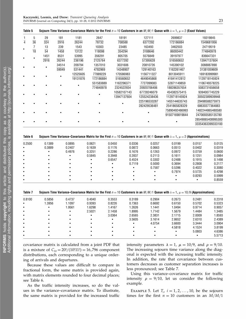
Rewriting the integral as a sum via Theorem 2avoids the calls to Convolution(X,Y) in APPL aswell as the need to integrate for each case andpiece. One can always use this approach, even whenthe independent part of a particular customer’ssojourn time contains many independent distribu-tion segments. The times for these segments can onlybe exponential4�+�5 distributed or exponential4�5distributed, which implies that their sum can alwaysbe written as the sum of two independent Erlangrandom variables. This approach speeds computationtime considerably. The symmetric variance–covariancematrix for n = 10 customers with parameters �= 1,� = 2, and �= 1/2 is showcased in Table 5; exact val-ues are provided.

CPU time is a factor in these computations.Each element in the 10th column of the variance–

INFORMS

holds

copyrightto

this

article

and

distrib

uted

this

copy

asa

courtesy

tothe

author(s).

Add

ition

alinform

ation,

includ

ingrig

htsan

dpe

rmission

policies,

isav

ailableat

http://journa

ls.in

form

s.org/.


Table 5 Sojourn Time Variance–Covariance Matrix for the First n = 10 Customers in an M/M/1 Queue with �= 1, �= 2 (Exact Values)

14

536

29324

1812916

118126244

264778732

18191708588

1271116377292

2699837172186884

193198451549681956

•718

1354

2391458

154313122

10303118098

23485354294

1634933188646

346250386093442

24719519774840978

• •14512916

853126244

53995236196

3562912125764

8057056377292

557684957395628

39197977516560652

83664733113947137604

• • •3451459049

209794531441

13570104782969

303160614348907

20810726129140163

1453901021162261467

308888789031381059609

• • • •1252560519131876

77889229172186884

170586983516560652

11567113274649045868

801304591141841412812

1691839999811129718145924

• • • • •551583889774840978

11622963712324522934

772709908320920706406

52871149859188286357654

11067493782255083731656658

• • • • • •1058210714313947137604

67728246079125524238436

4543825754151129718145924

939400774522930502389939948

• • • • • • •225196533287282429536481

14551446357432541865828329

2949858827597368630377364883

• • • • • • • •7589049248699391507169819844

14822448654805802470693585135780

• • • • • • • • •2854906540899530033354363399333100

Table 6 Sojourn Time Variance–Covariance Matrix for the First n = 10 Customers in an M/M/1 Queue with �= 1, �= 2 (Approximations)

0.2500 0.1389 0.0895 0.0621 0.0450 0.0336 0.0257 0.0199 0.0157 0.0125• 0.3889 0.2407 0.1639 0.1176 0.0872 0.0663 0.0513 0.0402 0.0319• • 004976 003251 0.2286 0.1676 0.1263 0.0972 0.0759 0.0600• • • 005845 0.3948 0.2837 0.2113 0.1611 0.1251 0.0984• • • • 0.6547 0.4524 0.3302 0.2488 0.1915 0.1498• • • • • 0.7119 0.5000 0.3694 0.2808 0.2177• • • • • • 0.7587 0.5396 0.4022 0.3080• • • • • • • 0.7974 0.5725 0.4298• • • • • • • • 0.8293 0.5999• • • • • • • • • 0.8559

Table 7 Sojourn Time Variance–Covariance Matrix for the First n = 10 Customers in an M/M/1 Queue with �= 1, �= 10/9 (Approximations)

0.8100 0.5856 0.4737 0.4040 0.3553 0.3189 0.2904 0.2673 0.2481 0.2318• 1.3956 1.1097 0.9393 0.8226 0.7363 0.6692 0.6150 0.5702 0.5323• • 1.9561 1.6298 1.4167 1.2626 1.1441 1.0494 0.9714 0.9057• • • 2.5021 2.1458 1.8995 1.7142 1.5679 1.4484 1.3485• • • • 3.0364 2.6565 2.3831 2.1715 2.0009 1.8593• • • • • 3.5605 3.1614 2.8652 2.6310 2.4389• • • • • • 4.0754 3.6600 3.3444 3.0904• • • • • • • 4.5818 4.1524 3.8199• • • • • • • • 5.0803 4.6386• • • • • • • • • 5.5713

covariance matrix is calculated from a joint PDF thatis a mixture of C10 = 20!/410!11!5 = 161796 componentdistributions, each corresponding to a unique order-ing of arrivals and departures.

Because these values are difficult to compare infractional form, the same matrix is provided again,with matrix elements rounded to four decimal places;see Table 6.

As the traffic intensity increases, so do the val-ues in the variance–covariance matrix. To illustrate,the same matrix is provided for the increased traffic

intensity parameters � = 1, � = 10/9, and � = 9/10.The increasing sojourn time variance along the diag-onal is expected with the increasing traffic intensity.In addition, the rate that covariance between cus-tomers decreases as customer separation increases isless pronounced; see Table 7.

Using this variance–covariance matrix for trafficintensity � = 9/10, let us consider the followingexample.

Example 5. Let Ti, i = 1121 0 0 0 110, be the sojourntimes for the first n = 10 customers in an M/M/1

INFORMS

holds

copyrightto

this

article

and

distrib

uted

this

copy

asa

courtesy

tothe

author(s).

Add

ition

alinform

ation,

includ

ingrig

htsan

dpe

rmission

policies,

isav

ailableat

http://journa

ls.in

form

s.org/.


Table 8 Sojourn Time Variance–Covariance Matrix for the First n = 10 Customers in an M/M/1 Queue with �= 1, �= 2/3 (Approximations)

2.2500 1.8900 1.7172 1.6135 1.5438 1.4937 1.4558 1.4263 1.4027 1.3835• 4.1400 3.7368 3.5018 3.3459 3.2344 3.1507 3.0856 3.0337 2.9913• • 6.0957 5.6825 5.4166 5.2292 5.0896 4.9817 4.8958 4.8261• • • 8.1312 7.7208 7.4397 7.2332 7.0747 6.9493 6.8479• • • • 10.2424 9.8410 9.5538 9.3361 9.1652 9.0276• • • • • 12.4235 12.0342 11.7463 11.5230 11.3444• • • • • • 14.6687 14.2931 14.0081 13.7828• • • • • • • 16.9727 16.6115 16.3319• • • • • • • • 19.3310 18.9846• • • • • • • • • 21.7397

queue, with arrival rate � = 1 and service rate � =

10/9, that is initially empty and idle. Find the varianceof the average sojourn time for the first 10 customers.

Define the average sojourn time as

±T =1

10

10∑

i=1

Ti0

Because the sojourn times are not independent ran-dom variables, the variance of the average sojourntime is

Var6±T 7 = Var[

110

10∑

i=1

Ti

]

=1

100 Var[ 10∑

i=1

Ti

]

=1

100

[ 10∑

i=1

Var6Ti7+ 2∑∑

i<j

Cov4Ti1Tj5]

0

The result is the sum of all elements in the variance–covariance matrix in Table 7 multiplied by the con-stant 1/100. The sum of the variance–covariancematrix rounded to four significant digits is 177.6642;therefore the variance of ±T is

Var6±T 7≈ 1077660

To verify the calculation a Monte Carlo simulationwas conducted five times, using one million replica-tions each time. The resulting 95% confidence intervalfor the variance of ±T was ±T ∈ 4107731107815, whichagrees with the analytic result.

Traditional steady-state queueing theory and anal-ysis lacks the insight provided in these transientvariance–covariance matrices. For businesses wherethe number of customers in a day is so small thattrue steady state is never achieved, routine queue-ing measures of performance are not representative ofreality. Additionally, consider a system where the traf-fic intensity exceeds 1. For such a system, an analystmight be interested in customer covariance. Increas-ing the traffic intensity so that � > 1 does not pre-clude covariance calculations using this method andtherefore allows transient analysis of such systems.

A variance–covariance matrix for � = 1, � = 2/3, and� = 3/2 is presented in Table 8. Given this trafficintensity, the system is unstable, and the expectedsojourn times for successive customers increase with-out bound. Along the main diagonal the customervariance is clearly increasing, and the covariancedecreases as the separation occurs between customers.This decrease is monotonic, and although not studiedin detail here, it appears that the rate of covariancedecrease might be of interest for an unstable trafficintensity.

7. Sojourn Time Covariance with kCustomers Initially Present

When k customers are present in the M/M/1 queueat time 0, the approach used to compute sojourntime covariance between customers becomes moredifficult. When the two customers of interest possessindices larger than k (i.e., Ti where i > k), then theapproach is similar to that derived in §6. However,there are two other possibilities. The first possibilityis that the first customer has an index of k or less,and the second customer has an index larger than k.In this instance, the only difference in deriving thejoint CDF is that the lower-indexed customer beginshis sojourn time at time 0. In the second possibility,both customers have an index of k or below. If theseindices are i and j , where i < j ≤ k, the time intervalsfor sojourn times Ti and Tj begin at 0. It is obvious thatTi ≤ Tj , because the completion time for customer imust occur prior to the completion time for cus-tomer j . For each of these possibilities, the covariancederivation that follows will mirror the empty and idlecovariance derivation in §6. To illustrate the calcula-tions, consider an M/M/1 queue with k = 2 customersinitially present at time 0 and a single additional cus-tomer, n = 1. The transition diagram where the firstevent (not including the k customers initially presentat time 0) is an arrival, which is analogous to Fig-ures 9 and 10, is given in Figure 12. The total numberof customers passing through the system is n+ k = 3.Using a “1” to denote an arrival and a “−1′′ to denotea departure, each arrival/departure ordering instancefor n+k = 3 customers must contain exactly three −1s

INFORMS

holds

copyrightto

this

article

and

distrib

uted

this

copy

asa

courtesy

tothe

author(s).

Add

ition

alinform

ation,

includ

ingrig

htsan

dpe

rmission

policies,

isav

ailableat

http://journa

ls.in

form

s.org/.


Arrival

Arrival

Arrival Departure

Departure

Departure

Figure 12 Transition Diagram for n + k = 1+ 2 = 3 Customers Whenthe First Event Is an Arrival

(completions of service) and a single 1 (arrival). Thealgorithm presented by Ruskey and Williams (2008)does not facilitate the listing of all orderings for anunbalanced system, where the number of departuresis greater than the number of arrivals (as opposed toan empty and idle queue at time 0). However, wecan produce all possible arrival/departure sequenceswith a simple manipulation of the algorithm as wellas count the number of possible sequences. The num-ber of possible orderings, denoted by C4n � k5, follows,where n represents the number of customers passingthrough the system that arrive after time 0, and k isthe number of customers present at time 0:

C4n � k5=

�k/2�∑

j=0

4−15j(

k− j

j

)

Cn+k−j

for k = 011121 0 0 0 and n= 1121 0 0 0 1 where �·� denotesthe greatest integer function. The case matrix C isfound by applying the Ruskey and Williams (2008)algorithm for n + k customers and then deleting theinstances where the first k events do not correspondto arrivals. As seen previously, the case matrix forn+ k = 1 + 2 = 3 customers is

C =

1 −1 1 1 −1 −1

1 1 −1 1 −1 −1

1 −1 1 −1 1 −1

1 1 −1 −1 1 −1

1 1 1 −1 −1 −1

0

Rows 2, 4, and 5 correspond to the first k = 2 eventsbeing arrivals. Rows 1 and 3 must be deleted fromthe case matrix, because for each row, a completion ofservice occurs prior to the first two arrivals. Deletingthese rows results in the case matrix

C =

1 1 −1 1 −1 −1

1 1 −1 −1 1 −1

1 1 1 −1 −1 −1

1

with the remaining rows representing all possiblearrival/departure sequences. We can further simplify

c2c1

c1

a1 a3

a3

a2

a3

c3

T3

T3

T1

T2

T3

T1

T1

T2

T2 c3

c3

c2

c2

Case 3

Case 2

Case 1

Figure 13 Three Cases for k = 2 Initial Customers and a Single n = 1Additional Customer in an M/M/1 Queue

the case matrix by deleting the first k columns, result-ing in

C =

−1 1 −1 −1−1 −1 1 −1

1 −1 −1 −1

0

The rows of the case matrix correspond to the threecases shown in Figure 13.

The algorithm for computing the joint PDF, andsubsequently the covariance, of the sojourn timesof any two customers does not differ significantlyfrom the algorithm presented in §6. However, for thesojourn times T1 and T2 in Figure 13, a new theoremis introduced.

Theorem 3. LetX ∼ exponential4�15 and Y ∼ expon-ential4�25 be independent random variables. The joint PDFof 4T11T25= 4X1X +Y 5 is

fT11T24t11 t25= �1�2e

−�2t1−�1t2+�1t1 0 < t1 < t20

Proof. The joint CDF of T1 and T2 is

FT11T24t11 t25

= Pr4T1 ≤ t11T2 ≤ t25

= Pr4X ≤ t11X +Y ≤ t25

= Pr4X ≤ t11Y ≤ t2 −X5

=

∫ t1

0

∫ t2−x

0fX4x5 · fY 4y5dy dx

=

∫ t1

0

∫ t2−x

04�1e

−�1x5 · 4�2e−�2y5 dy dx

=�1 −�2 +�2e

−�1t2 +�2e−�2t1 −�1e

−�2t1 −�2e−�2t1−�1t2+�1t1

�1 −�21

for 0 < t1 < t2. Taking partial derivatives, fT11T24t11 t25 is

fT11T24t11 t25 = �1�2e

−�2t1−�1t2+�1t1 0 < t1 < t20 �

INFORMS

holds

copyrightto

this

article

and

distrib

uted

this

copy

asa

courtesy

tothe

author(s).

Add

ition

alinform

ation,

includ

ingrig

htsan

dpe

rmission

policies,

isav

ailableat

http://journa

ls.in

form

s.org/.


Theorem 3 provides the joint PDF for the sojourntimes T1 and T2 of the first two customers initiallypresent at time 0. It may be more complicated tocalculate the joint PDFs for the sojourn times ofother pairs of customers who were initially presentat time 0. This is because if 4i1 j5 6= 41125 and i <j ≤ k, where k is the number of customers presentat time 0, the time intervals of duration X and Yduring which customers i and j , respectively, areserved may each be composed of multiple indepen-dent, exponentially distributed time segments. Eachof these multiple segments is limited to only one oftwo possibilities, an exponential4�+�5 segment or anexponential4�5 segment. In this more complicated sit-uation, we let 4Ti1Tj5 = 4X1X + Y 5, as in Theorem 3,and apply Theorem 2 to find the PDFs of X and Y(using the procedure conv(m,n)); we then let Maplehandle the sojourn time joint PDF calculation. Whenthe second customer of interest has an index greaterthan or equal to k, the sojourn time joint PDF followsan application of Theorem 1 as described in §6, whencases exist with dependence.

Using the final case matrix C above, the associatedsegment distribution matrix C ′ is

C ′=

1 1 2 21 1 0 21 2 2 2

1

where the possible elements are the same as definedin §6. The probability vector associated with the casematrix C is

[

29

49

13

]

for arrival rate �= 1 and service rate �= 2.Using the case matrix C and the segment distribu-

tion matrix C ′, the joint PDFs for each case are createdby selecting the appropriate segments for a given pairof customers, where the segments are identified bythe Rl matrix discussed in §6. Once the joint PDFs arecreated for each case, they are mixed with the proba-bility vector to determine the sojourn time joint PDFfor covariance calculations. These calculations arecoded in Maple as the procedure kCov(X,Y,a,b,n,k).The first two arguments X and Y are the distribu-tion of time between arrivals, exponential4�5, and theservice time distribution, exponential4�5, respectively.They are entered in the APPL list-of-lists format. Thearguments a and b are the customers of interest for thecovariance calculation, where a < b. The argument nis the number of customers processing through thesystem not including those present at time 0, whichis indicated by the last argument k. Therefore, thetotal number of customers processing through thesystem is n+ k, and a covariance calculation betweenany two of these customers can be achieved with theappropriate function call. For example, the functioncall kCov(ExponentialRV(1), ExponentialRV(2), 1,2,1,3) calculates the covariance between customers 1

and 2 in an M/M/1 queue with an arrival rate �= 1,service time rate � = 2, three customers present attime 0, and a single additional customer processingthrough the system. The variance–covariance matrixfor an M/M/1 queue with an arrival rate �= 1 andservice rate � = 2, where k = 4 customers are presentat time 0 and an additional n = 6 customers processthrough the system, is presented in Table 9.

Unlike the previous variance–covariance matrices,some row elements—in particular, those elementsassociated with customers who are initially present—do not decrease monotonically. To explain theseentries, consider Theorem 4.

Theorem 4. If X11X21 0 0 0 1Xn are iid exponential4�5random variables and

Ts =

s∑

r=1

Xr s = 1121 0 0 0 1n1

then Var4Ti5= Cov4Ti1Tl5, 0 < i < l ≤ n.

Proof. Note that E6Tk7= k/� for k = 1121 0 0 0 1n andthat Ti and Xr are independent for 1 ≤ i < r ≤ n:

Cov4Ti1Tl5 = E

[(

Ti−i

�

)(

Tl−l

�

)]

= E

[(

Ti−i

�

){(

Ti−i

�

)

+

l∑

r=i+1

(

Xr −1�

)}]

= E

[(

Ti−i

�

)2]

+E

{ l∑

r=i+1

[(

Ti−i

�

)(

Xr −1�

)]}

= Var6Ti7+l∑

r=i+1

E

[

Ti−i

�

]

E

[

Xr −1�

]

= Var6Ti70 �

We can apply Theorem 4 to those customerpairs where both indices i1 j ≤ k. Therefore, theentries in the variance–covariance matrix for customerpairs 41125, 41135, and 41145 are

Var6T17= Cov4T11T25= Cov4T11T35= Cov4T11T45=14 0

Likewise, for the customer pairs 42135 and 42145,

Var6T27= Cov4T21T35= Cov4T21T45=12 0

Furthermore, it can be shown that, in general,

Var6Ti7= Cov4Ti1Tj5=i

�2

for i < j ≤ k, where k customers are present attime 0. For example, consider a single-server boxoffice with exponential4�5 service times that will be

INFORMS

holds

copyrightto

this

article

and

distrib

uted

this

copy

asa

courtesy

tothe

author(s).

Add

ition

alinform

ation,

includ

ingrig

htsan

dpe

rmission

policies,

isav

ailableat

http://journa

ls.in

form

s.org/.


Table 9 Sojourn Time Variance–Covariance Matrix for the First n = 6 Customers in an M/M/1 Queue with k = 4 Customers InitiallyPresent and �= 1, �= 2 (Exact Values)

14

14

14

14

211972

15798748

1165178732

28553236196

6301316377292

464615557395628

•12

12

12

211486

15794374

1165139366

28553118098

6301313188646

464615528697814

• •34

34

211324

15792916

1165126244

2855378732

6301312125764

464615519131876

• • • 1211243

15792187

1165119683

2855359049

6301311594323

464615514348907

• • • •3728926244

271153236196

19667772125764

15881532125764

3475520357395628

7638752811549681956

• • • • •16296551062882

116638879565938

93537439565938

203800469258280326

44653999916973568802

• • • • • •263490131172186884

208262483172186884

45062056334649045868

98323535707125524238436

• • • • • • •6393987843046721

13591892501162261467

2940206162231381059609

• • • • • • • •179260456277125524238436

3797217862633389154437772

• • • • • • • • •6270895566374545753584909922

offering tickets to a popular concert the next day. If1,000 patrons, each buying one ticket, camp out thenight before to get the best seats for the concert, thesek = 11000 customers are present at time 0, and there-fore we can predetermine the covariance between thesojourn times of any two of the customers. Addition-ally, Theorem 4 presents the counterintuitive resultthat Cov4T11T25 = Cov4T11T110005. As expected, thecorrelation decreases with increasing lag because ofthe diminishing effect of the intermediate customersojourn times reflected in the denominator of thedefining formula for correlation.

8. ConclusionPrevious transient analysis results for the M/M/1and M/M/s queues have been combined with thefunctionality of the Maple computational engine (andsubsequently APPL) to develop both symbolic andnumeric exact sojourn time PDFs that can be manipu-lated to compute and study various measures of per-formance. A complete variance–covariance matrix forthe first n= 10 customers and varying traffic inten-sity is calculated, which illustrates this approach’sability to determine the joint PDF between twocustomer sojourn times. The results offer a frame-work for describing how the well-known M/M/squeue steady-state results occur as the queue pro-gresses toward steady state. When possible, results

are checked against corresponding Monte Carlo sim-ulation and/or previous literature. The first princi-ple’s derivation suggests that a viable alternative forfuture research would be to apply the approachesprovided in this work to a G/G/1 queue. Compu-tational considerations take priority as n increases.Making use of other computational formulae (suchas Hagwood 2009) may offer significant time savingsand is another interesting avenue for future work.

AcknowledgmentsThe authors thank Bert Zwart for describing the conditionaldiscrete-event model in Figure 6. They thank Sheldon Rossfor offering his assistance in the covariance and correlationsections of this paper. The authors also thank Sid Lawrence,Barry Nelson, Raghu Pasupathy, and Bruce Schmeiser fortheir assistance in deriving the sojourn time distributions.

ReferencesAbate, J., W. Whitt. 1988. Transient behavior of the M/M/1 queue

via Laplace transforms. Adv. Appl. Probab. 20(1) 145–178.de Souza e Silva, E. S., H. R. Gail, R. V. Campos. 1995. Calculating

transient distributions of cumulative reward. B. D. Gaither, ed.Proc. 1995 ACM SIGMETRICS Joint Internat. Conf. MeasurementModel. Comput. Systems, ACM, New York, 231–240.

Gafarian, A. V., C. J. Ancker Jr., T. Morisaku. 1976. The problemof the initial transient in digital computer simulation. Proc. 76Bicentennial Conf. Winter Simul., Gaithersburg, MD, 49–51.

Glen, A. G., D. L. Evans, L. M. Leemis. 2001. APPL: A probabilityprogramming language. Amer. Statistician 55(2) 156–166.

Grassmann, W. K. 1977. Transient solutions in Markovian queueingsystems. Comput. Oper. Res. 4(1) 47–53.

INFORMS

holds

copyrightto

this

article

and

distrib

uted

this

copy

asa

courtesy

tothe

author(s).

Add

ition

alinform

ation,

includ

ingrig

htsan

dpe

rmission

policies,

isav

ailableat

http://journa

ls.in

form

s.org/.


Grassmann, W. K. 2008. Warm-up periods in simulation can bedetrimental. Probab. Engrg. Inform. Sci. 22(3) 415–429.

Hagwood, C. 2009. An application of the residue calculus: Thedistribution of the sum of nonhomogeneous gamma variates.Amer. Statistician 63(1) 37–39.

Hillier, F. S., G. J. Lieberman. 2005. Introduction to OperationsResearch. McGraw-Hill, New York.

Hogg, R. V., A. T. Craig, J. McKean. 2005. Introduction to Mathemat-ical Statistics. Macmillan, New York.

Kelton, W. D. 1985. Transient exponential—Erlang queues andsteady-state simulation. Comm. ACM 28(7) 741–749.

Kelton, W. D., A. M. Law. 1985. The transient behavior of theM/M/s queue, with implications for steady-state simulation.Oper. Res. 33(2) 378–396.

Kleinrock, L. 1975. Queueing Systems. John Wiley & Sons, New York.Law, A. M. 1975. A comparison of two techniques for determin-

ing the accuracy of simulation output. Technical Report 75–11,University of Wisconsin–Madison, Madison.

Leguesdron, P., J. Pellaumail, G. Rubino, B. Sericola. 1993. Transientanalysis of the M/M/1 queue. Adv. Appl. Probab. 25(3) 702–713.

Morisaku, T. 1976. Techniques for data-truncation in digitalcomputer simulation. Ph.D. thesis, University of SouthernCalifornia, Los Angeles.

Odoni, A. R., E. Roth. 1983. An empirical investigation of the tran-sient behavior of stationary queueing systems. Oper. Res. 31(3)432–455.

Parthasarathy, P. R. 1987. A transient solution to an M/M/1 queue:A simple approach. Adv. Appl. Probab. 19(4) 997–998.

Pegden, C. D., M. Rosenshine. 1982. Some new results for theM/M/1 queue. Management Sci. 28(7) 821–828.

Ruskey, F., A. Williams. 2008. Generating balanced parenthesesand binary trees by prefix shifts. J. Harland, P. Manyem,eds. Proc. 14th Sympos. Comput.: Australasian Theory, Vol. 77.Australian Computer Society, Darlinghurst, NSW, Australia,107–115.

Stanley, R. P. 1999. Enumerative Combinatorics: Volume 2. CambridgeStudies in Advanced Mathematics, Vol. 62. Cambridge Univer-sity Press, Cambridge, UK.

Winston, W. L. 2004. Operations Research: Applications and Algorithms.Thomson, Belmont, CA.

INFORMS

holds

copyrightto

this

article

and

distrib

uted

this

copy

asa

courtesy

tothe

author(s).

Add

ition

alinform

ation,

includ

ingrig

htsan

dpe

rmission

policies,

isav

ailableat

http://journa

ls.in

form

s.org/.

Documents

Transient Queueing Analysis - William & Maryleemis/2012informsjocb.pdfThe trafﬁc intensity of the system is ’D‰=s„. The system consists of a single queue with customers waiting