Embed Size (px)
Citation preview

TRANSFORMERDESIGN PRINCIPLES
With Applications toCore-Form Power Transformers
Robert M.Del VecchioBertrand PoulinPierre T.Feghali
Dilipkumar M.ShahRajendra Ahuja
Boca Raton London New York Washington, D.C.
CRC PRESS
© 2002 by CRC Press

This book contains information obtained from authentic and highly regarded sources.Reprinted material is quoted with permission, and sources are indicated. A widevariety of references are listed. Reasonable efforts have been made to publish reliabledata and information, but the authors and the publisher cannot assume responsibilityfor the validity of all materials or for the consequences of their use.
Neither this book nor any part may be reproduced or transmitted in any form or byany means, electronic or mechanical, including photocopying, microfilming, andrecording, or by any information storage or retrieval system, without prior permissionin writing from the publisher.
The consent of CRC Press does not extend to copying for general distribution, forpromotion, for creating new works, or for resale. Specific permission must be obtainedin writing from CRC Press for such copying.
Direct all inquiries to CRC Press, 2000 N.W. Corporate Blvd., Boca Raton, Florida33431.
Trademark Notice: Product or corporate names may be trademarks or registeredtrademarks, and are used only for identification and explanation, without intent toinfringe.
Visit the CRC Press Web site at www.crcpress.com
© 2002 by CRC Press
No claim to original U.S. Government worksInternational Standard Book Number 90-5699-703-3
Printed in the United States of America 1 2 3 4 5 6 7 8 9 0Printed on acid-free paper
© 2002 by CRC Press

CONTENTS
Preface xi
1 Introduction to Transformers 11.1 Historical Background 11.2 Uses in Power Systems 31.3 Core-Form and Shell-Form Transformers 91.4 Stacked and Wound Core Construction 101.5 Transformer Cooling 151.6 Winding Types 171.7 Insulation Structures 201.8 Structural Elements 241.9 Three-Phase Connections 291.10 Modern Trends 36
2 Transformer Circuit Models, Including Magnetic CoreCharacteristics and Applications 392.1 Introduction 392.2 Basic Magnetism 422.3 Hysteresis 462.4 Magnetic Circuits 492.5 Inrush Current 542.6 Transformer Circuit Model with Core 662.7 Per Unit System 802.8 Voltage Regulation 82
3 Reactance Calculations 873.1 Introduction 873.2 Ideal Transformers 88
3.2.1 Ideal Autotransformer 923.3 Leakage Impedance for 2-Winding Transformers 94
3.3.1 Leakage Impedance for a 2-WindingAutotransformer 98
3.4 Leakage Impedances for 3-Winding Transformers 993.4.1 Leakage Impedances for an
Autotransformer with Tertiary 104
© 2002 by CRC Press

CONTENTSvi
3.4.2 Leakage Impedance between 2 WindingsConnected in Series and a Third Winding 109
3.4.3 Leakage Impedance of a 2-WindingAutotransformer with X-Line Taps 110
3.4.4 More General Leakage Impedance Calculations 1133.5 Two Winding Leakage Reactance Formula 114
4 Fault Current Calculations 1194.1 Introduction 1194.2 Symmetrical Components 1214.3 Fault Analysis on 3-Phase Systems 127
4.3.1 3-Phase Line to Ground Fault 1294.3.2 Single Phase Line to Ground Fault 1304.3.3 Line to Line Fault 1314.3.4 Double Line to Ground Fault 132
4.4 Fault Currents for Transformers with 2 Terminalsper Phase 1334.4.1 3-Phase Line to Ground Fault 1354.4.2 Single Phase Line to Ground Fault 1364.4.3 Line to Line Fault 1374.4.4 Double Line to Ground Fault 1374.4.5 Zero Sequence Impedences 138
4.5 Fault Currents for Transformers with 3 Terminalsper Phase 1404.5.1 3-Phase Line to Ground Fault 1434.5.2 Single Phase Line to Ground Fault 1434.5.3 Line to Line Fault 1444.5.4 Double Line to Ground Fault 1454.5.5 Zero Sequence Impedances 146
4.6 Asymmetry Factor 147
5 Rabins’ Method for Calculating Leakage Fields, Forces andInductances in Transformers 1495.1 Introduction 1495.2 Theory 1505.3 Determining the B-Field 1665.4 Determing the Winding Forces 1675.5 General Method for Determing Inductances and Mutual
Inductances 1695.6 Rabins’ Formula for Leakage Reactance 1755.7 Rabins’ Method Applied to Calculate Self and Mutual
Inductances of Coil Sections 182
© 2002 by CRC Press
CONTENTS vii
6 Mechanical Design 1856.1 Introduction 1856.2 Force Calculations 1886.3 Stress Analysis 190
6.3.1 Compressive Stress in the Key Spacers 1936.3.2 Axial Bending Stress per Strand 1936.3.3 Tilting Strength 1976.3.4 Stress in Tie Bars 2016.3.5 Stress in the Pressure Rings 2086.3.6 Hoop Stress 2096.3.7 Radial Bending Stress 211
6.4 Radial Buckling Strength 2196.5 Stress Distribution in a Composite Wire-Paper
Winding Section 2296.6 Additional Mechanical Considerations 235
7 Capacitance Calculations 2377.1 Introduction 2377.2 Theory 2387.3 Stein’s Capacitance Formula 2457.4 General Disk Capacitance Formula 2527.5 Coil Grounded at One End with Grounded
Cylinders on Either Side 2537.6 Static Ring on One Side of Disk 2567.7 Terminal Disk without a Static Ring 2577.8 Capacitance Matrix 2587.9 Two End Static Rings 2617.10 Static Ring between the First Two Disks 2657.11 Winding Disk Capacitances with Wound-in Shields 266
7.11.1 Analytic Formula 2667.11.2 Circuit Model 2707.11.3 Experimental Methods 2767.11.4 Results 277
7.12 Multi-Start Winding Capacitance 281
8 High Voltage Insulation Design 2858.1 Introduction 2858.2 Principles of Voltage Breakdown 2868.3 Insulation Coordination 2988.4 Continuum Model of Winding Used to Obtain
the Impulse Voltage Distribution 303
© 2002 by CRC Press

CONTENTSviii
8.5 Lumped Parameter Model for TransientVoltage Distribution 3138.5.1 Circuit Description 3138.5.2 Mutual and Self Inductance Calculations 3178.5.3 Capacitance Calculations 3198.5.4 Impulse Voltage Calculations and
Experimental Comparisons 3208.5.5 Sensitivity Studies 326
9 Electric Field Calculations 3299.1 Simple Geometries 3299.2 Electric Field Calculations Using Conformal Mapping 337
9.2.1 Physical Basis 3379.2.2 Conformal Mapping 3389.2.3 Schwarz-Christoffel Transformation 3429.2.4 Conformal Map for the Electrostatic
Field Problem 3449.2.4.1 Electric Potential and Field Values 3499.2.4.2 Calculations and Comparison with
a Finite Element Solution 3569.2.4.3 Estimating Enhancement Factors 360
9.3 ‘Finite Element Electric Field Calculations 363
10 Losses 36910.1 Introduction 36910.2 No-Load or Core Losses 370
10.2.1 Building Factor 37510.2.2 Interlaminar Losses 375
10.3 Load Losses 37910.3.1 I2R Losses 37910.3.2 Stray Losses 380
10.3.2.1 Eddy Current Losses in the Coils 38310.3.2.2 Tieplate Losses 38710.3.2.3 Tieplate and Core Losses Due to
Unbalanced Currents 39710.3.2.4 Tank and Clamp Losses 40410.3.2.5 Tank Losses Due to Nearby Busbars 40710.3.2.6 Tank Losses Associated with
the Bushings 41210.3.3 Winding Losses Due to Missing
or Unbalanced Crossovers 418
© 2002 by CRC Press

CONTENTS ix
11 Thermal Model of a Core Form Power Transformerand Related Thermal Calculations 42911.1 Introduction 42911.2 Thermal Model of a Disk Coil with Directed
Oil Flow 43111.2.1 Oil Pressures and Velocities 43311.2.2 Oil Nodal Temperatures and Path
Temperature Rises 43811.2.3 Disk Temperatures 440
11.3 Thermal Model for Coils without Directed Oil Flow 44111.4 Radiator Thermal Model 44411.5 Tank Cooling 44811.6 Oil Mixing in the Tank 45011.7 Time Dependence 45311.8 Pumped Flow 45411.9 Comparison with Test Results 45511.10 Determining M and N Exponents 46011.11 Loss of Life Calculation 46211.12 Cable and Lead Temperature Calculation 46611.13 Tank Wall Temperature Calculation 47311.14 Tieplate Temperature Calculation 47511.15 Core Steel Temperature Calculation 478
12 Load Tap Changers 48112.1 Introduction 48112.2 General Description of LTC 48212.3 Types of Regulation 48312.4 Principle of Operation 484
12.4.1 Resistive Switching 48412.4.2 Reactive Switching with Preventative
Autotransformer 48612.5 Connection Schemes 488
12.5.1 Full Transformers 48812.5.2 Autotransformers 49012.5.3 Use of Auxiliary Transformer 49312.5.4 Phase Shifting Transformers 495
12.6 General Maintenance 495
13 Phase Shifting Transformers 49913.1 Introduction 49913.2 Basic Principles 503
© 2002 by CRC Press

CONTENTSx
13.3 Squashed Delta Phase Shifting Transformers 50713.4 Standard Delta Phase Shifting Transformers 51413.5 Two Core Phase Shifting Transformer 51913.6 Regulation Effects 52613.7 Fault Current Analysis 528
13.7.1 Squashed Delta Fault Currents 53213.7.2 Standard Delta Fault Currents 535
14 Cost Minimization 54314.1 Introduction 54314.2 Geometric Programming 54514.3 Non-Linear Constrained Optimization 552
14.3.1 Characterization of the Minimum 55214.3.2 Solution Search Strategy 56114.3.3 Practical Considerations 567
14.4 Application to Transformer Design 56814.4.1 Design Variables 56914.4.2 Cost Function 57014.4.3 Equality Constraints 57314.4.4 Inequality Constraints 57714.4.5 Optimization Strategy 578
References 583
© 2002 by CRC Press

PREFACEMany of the standard texts on power transformers are now over tenyears old and some much older. Much has changed in transformer designsince these books were written. Newer and better materials are nowavailable for core and winding construction. Powerful computers nowmake it possible to produce more detailed models of the electrical,mechanical and thermal behavior of transformers than previouslypossible. Although many of these modern approaches to design andconstruction are found scattered in the literature, there is a need to havethis information available in a single source as a reference for the designeror power engineer and as a starting point for the student or novice.
It is hoped that the present work can serve both purposes. As a text forbeginners, we emphasize the physical basis of transformer operation. Wealso discuss the physical effects which result from various fault conditionsand their implications for design. Physical principles and mathematicaltechniques are presented in a reasonably self-contained manner, althoughreferences are provided to additional material. For the specialist such asa power or transformer design engineer, detailed models are presentedwhich focus on various aspects of a transformer under normal orabnormal conditions. Cost minimization techniques, which form thestarting point for most designs, are also presented.
Although this book primarily deals with power transformers, manyof the physical principles discussed or mathematical modelingtechniques presented apply equally well to other types of transformers.The presentation is kept as general as possible so that designers or usersof other transformer types will have little difficulty applying many ofthe results to their own designs. The emphasis on fundamentals shouldmake this process easier and should also foster the development of newand more powerful design tools in the future.
The International System of Units (SI) is used throughout the text.However, an occasional figure, graph, or table may show quantities inthe British system of units. Sometimes a quantity is given in British unitsin parentheses after its metric value.
References are referred to generally by the first three letters of the firstauthor’s name followed by the last two digits of the publication date, e.g.[Abc98]. In cases where this format cannot be followed, an appropriatesubstitute is made. They are listed alphabetically at the end of the book.
We wish to thank Harral Robin for guidance throughout the course ofthis work. We would also like to acknowledge many helpful suggestionsfrom power industry representatives and consultants over the years.
© 2002 by CRC Press

1
1. INTRODUCTION TOTRANSFORMERS
Summary Beginning with the principle of induction discovered byFaraday, the transformer slowly evolved to fill a need in electricalpower systems. The development of 3 phase a.c. power has led to agreat variety of transformer types, We discuss some of these typesand their use in power systems. We also discuss and contrast some ofthe main construction methods. The principle components of atransformer are highlighted with special emphasis on core-form powertransformers. Some of the basic considerations which determine thedesign of these components are presented. A look at some newertechnologies is given which could impact the future development oftransformers.
1.1 HISTORICAL BACKGROUND
Transformers are electrical devices which change or transform voltagelevels between two circuits. In the process, current values are alsotransformed. However, the power transferred between the circuits isunchanged, except for a typically small loss which occurs in the process.This transfer only occurs when alternating current (a.c.) or transientelectrical conditions are present. Transformer operation is based on theprinciple of induction discovered by Faraday in 1831. He found thatwhen a changing magnetic flux links a circuit, a voltage or electromotiveforce (emf) is induced in the circuit. The induced voltage is proportionalto the number of turns linked by the changing flux. Thus when twocircuits are linked by a common flux and there are different linked turnsin the two circuits, there will be different voltages induced. This situationis shown in Fig. 1.1 where an iron core is shown carrying the commonflux. The induced voltages V1 and V2 will differ since the linked turns N1
and N2 differ.
© 2002 by CRC Press

INTRODUCTION2
Devices based on Faraday’s discovery, such as inductors, were littlemore than laboratory curiosities until the advent of a.c. electricalsystems for power distribution which began towards the end of thenineteenth century. Actually the development of a.c. power systems andtransformers occurred almost simultaneously since they are closelylinked. The invention of the first practical transformer is attributed tothe Hungarian engineers Karoly Zipernowsky, Otto Blathy, and MiksaDeri in 1885 [Jes97]. They worked for the Hungarian Ganz factory.Their device had a closed toroidal core made of iron wire. The primaryvoltage was a few kilo volts and the secondary about 100 volts. It wasfirst used to supply electric lighting.
Modern transformers differ considerably from these early models butthe operating principle is still the same. In addition to transformers usedin power systems which range in size from small units which are attachedto the tops of telephone poles to units as large as a small house andweighing hundreds of tons, there are a myriad of transformers used in theelectronics industry. These latter range in size from units weighing a fewpounds and used to convert electrical outlet voltage to lower values
Figure 1.1 Transformer principle illustrated for two circuits linked by a commonchanging flux
© 2002 by CRC Press

INTRODUCTION 3
required by transistorized circuitry to micro-transformers which aredeposited directly onto silicon substrates via lithographic techniques.
Needless to say, we will not be covering all these transformer typeshere in any detail, but will instead focus on the larger powertransformers. Nevertheless, many of the issues and principles discussedare applicable to all transformers.
1.2 USES IN POWER SYSTEMS
The transfer of electrical power over long distances becomes moreefficient as the voltage level rises. This can be seen by considering asimplified example. Suppose we wish to transfer power P over a longdistance. In terms of the voltage V and line current I, this power can beexpressed as
P=VI (1.1)
where rms values are assumed and the voltage and current are assumedto be in phase. For a line of length L and cross-sectional area A, itsresistance is given by
(1.2)
where ρ is the electrical resistivity of the line conductor. The electricallosses are therefore
(1.3)
and the voltage drop is
(1.4)
Substituting for I from (1.1), we can rewrite the loss and voltagedrop as
(1.5)
© 2002 by CRC Press

INTRODUCTION4
Since P, L, ρ are assumed given, the loss and voltage drop can be madeas small as desired by increasing the voltage V. However, there arelimits to increasing the voltage, such as the availability of adequateand safe insulation structures and the increase of corona losses.
We also notice from (1.5) that increasing the cross-section area of theline conductor A can lower the loss and voltage drop. However as Aincreases, the weight of the line conductor and therefore its cost alsoincrease so that a compromise must be reached between the cost oflosses and acceptable voltage drop and the conductor material costs.
In practice, long distance power transmission is accomplished withvoltages in the range of 100–500 kV and more recently with voltages ashigh as 765 kV. These high voltages are, however, incompatible with safeusage in households or factories. Thus the need for transformers isapparent to convert these to lower levels at the receiving end. In addition,generators are, for practical reasons such as cost and efficiency, designedto produce electrical power at voltage levels of ~10 to 40 kV. Thus thereis also a need for transformers at the sending end of the line to boost thegenerator voltage up to the required transmission levels. Fig. 1.2 shows asimplified version of a power system with actual voltages indicated. GSUstands for generator step-up transformer.
In modern power systems, there is usually more than one voltagestep-down from transmission to final distribution, each step downrequiring a transformer. Fig. 1.3 shows a transformer situated in aswitch yard. The transformer takes input power from a high voltageline and converts it to lower voltage power for local use. The secondarypower could be further stepped down in voltage before reaching thefinal consumer. This transformer could supply power to a large numberof these smaller step down transformers. A transformer of the sizeshown could support a large factory or a small town.
Figure 1.2 Schematic drawing of a power system
© 2002 by CRC Press

INTRODUCTION 5
There is often a need to make fine voltage adjustments tocompensate for voltage drops in the lines and other equipment. Thesevoltage drops depend on the load current so they vary throughout theday. This is accomplished by equipping transformers with tap changers.These are devices which add or subtract turns from a winding, thusaltering its voltage. This process can occur under load conditions orwith the power disconnected from the transformer. The correspondingdevices are called respectively load or no-load tap changers. Load tapchangers are typically sophisticated mechanical devices which can beremotely controlled. The tap changes can be made to occurautomatically when the voltage levels drop below or rise above certainpredetermined values. Maintaining nominal or expected voltage levelsis highly desirable since much electrical equipment is designed tooperate efficiently and sometimes only within a certain voltage range.This is particularly true for solid state equipment. No-load tapchanging is usually performed manually. This type of tap changing canbe useful if long term drifts are occurring in the voltage level. Thus it isdone infrequently. Fig. 1.4 shows three load tap changers and their
Figure 1.3 Transformer located in a switching station, surrounded by auxiliary equipment
© 2002 by CRC Press

INTRODUCTION6
connections to three windings of a power transformer. The sametransformer can be equipped with both types of tap changers.
Most power systems today are three phase systems, i.e. they producesinusoidal voltages and currents in three separate circuits which aredisplaced in time relative to each other by 1/3 of a cycle or 120 electricaldegrees as shown in Fig. 1.5. Note that, at any instant of time, the 3voltages sum to zero. Such a system made possible the use of generatorsand motors without commutators which were cheaper and safer tooperate. Thus transformers were required which transformed all 3 phasevoltages. This could be accomplished by using 3 separate transformers,one for each phase, or more commonly by combining all 3 phases withina single unit, permitting some economies particularly in the corestructure. A sketch of such a unit is shown in Fig. 1.6. Note that the threefluxes produced by the different phases are, like the voltages and currents,displaced in time by 1/3 of a cycle relative to each other. This means that,when they overlap in the top or bottom yokes of the core, they canceleach other out. Thus the yoke steel does not have to be designed to carrymore flux than is produced by a single phase.
Figure 1.4 Three load tap changers attached to three windings of a power transformer.These tap changers were made by the Maschinenfabrik Reinhausen Co., Germany.
© 2002 by CRC Press

INTRODUCTION 7
At some stages in the power distribution system, it is desirable tofurnish single phase power. For example, this is the common form ofhousehold power. To accomplish this, only one of the output circuits of
Figure 1.5 Three phase voltages versus time.
Figure 1.6 Three phase transformer utilizing a 3 phase core
© 2002 by CRC Press

INTRODUCTION8
a 3 phase unit is used to feed power to a household or group ofhouseholds, The other circuits feed similar groups of households.Because of the large numbers of households involved, on average eachphase will be equally loaded.
Because modern power systems are interconnected so that power canbe shared between systems, sometimes voltages do not match atinterconnection points. Although tap changing transformers can adjustthe voltage magnitudes, they do not alter the phase angle. A phaseangle mismatch can be corrected with a phase shifting transformer.This inserts an adjustable phase shift between the input and outputvoltages and currents. Large power phase shifters generally require two3 phase cores housed in separate tanks. A fixed phase shift, usually of30°, can be introduced by suitably interconnecting the phases ofstandard 3 phase transformers, but this is not adjustable.
Transformers are fairly passive devices containing very few movingparts. These include the tap changers and cooling fans which areneeded on most units. Sometimes pumps are used on oil filledtransformers to improve cooling. Because of their passive nature,transformers are expected to last a long time with very littlemaintenance. Transformer lifetimes of 25–50 years are common. Oftenunits will be replaced before their useful life is up because ofimprovements in losses, efficiency, and other aspects over the years.Naturally a certain amount of routine maintenance is required. In oilfilled transformers, the oil quality must be checked periodically andfiltered or replaced if necessary. Good oil quality insures sufficientdielectric strength to protect against electrical breakdown. Keytransformer parameters such oil and winding temperatures, voltages,currents, and oil quality as reflected in gas evolution are monitoredcontinuously in many power systems. These parameters can then beused to trigger logic devices to take corrective action should they falloutside of acceptable operating limits. This strategy can help prolongthe useful operating life of a transformer. Fig. 1.7 shows the end of atransformer tank where a control cabinet is located which houses themonitoring circuitry. Also shown projecting from the sides are radiatorbanks equipped with fans. This transformer is fully assembled and isbeing moved to the testing location in the plant.
© 2002 by CRC Press

INTRODUCTION 9
1.3 CORE-FORM AND SHELL-FORM TRANSFORMERS
Although transformers are primarily classified according to their functionin a power system, they also have subsidiary classifications accordingto how they are constructed. As an example of the former type ofclassification, we have generator step-up transformers which are connecteddirectly to the generator and raise the voltage up to the line transmissionlevel or distribution transformers which are the final step in a powersystem, transferring single phase power directly to the household orcustomer. As an example of the latter type of classification, perhaps themost important is the distinction between core-form and shell-formtransformers.
The basic difference between a core-form and shell-form transformeris illustrated in Fig. 1.8. In a core-form design, the coils are wrapped orstacked around the core. This lends itself to cylindrical shaped coils.Generally high voltage and low voltage coils are wound concentrically,with the low voltage coil inside the high voltage one. In the 2 coil splitshown in Fig. 1.8a, each coil group would consist of both high and lowvoltage windings. This insures better magnetic coupling between thecoils. In the shell form design, the core is wrapped or stacked around thecoils. This lends itself to flat oval shaped coils called pancake coils,
Figure 1.7 End view of a transformer tank showing the control cabinet which housesthe electronics.
© 2002 by CRC Press

INTRODUCTION10
with the high and low voltage windings stacked on top of each other,generally in more than one layer each in an alternating fashion.
Each of these types of construction has its advantages anddisadvantages. Perhaps the ultimate determination between the twocomes down to a question of cost. In distribution transformers, the shellform design is very popular because the core can be economicallywrapped around the coils. For moderate to large power transformers,the core-form design is more common, possibly because the short circuitforces can be better managed with cylindrically shaped windings.
1.4 STACKED AND WOUND CORE CONSTRUCTION
In both core-form and shell-form types of construction, the core is madeof thin layers or laminations of electrical steel, especially developed forits good magnetic properties. The magnetic properties are best alongthe rolling direction so this is the direction the flux should naturallywant to take in a good core design. The laminations can be wrappedaround the coils or stacked. Wrapped or wound cores have few, if any,joints so they carry flux nearly uninterrupted by gaps. Stacked coreshave gaps at the corners where the core steel changes direction. Thisresults in poorer magnetic characteristics than for wound cores. In largerpower transformers, stacked cores are much more common while insmall distribution transformers, wound cores predominate. The
Figure 1.8 Single phase core-form and shell-form transformers contrasted
© 2002 by CRC Press

INTRODUCTION 11
laminations for both types of cores are coated with an insulating coatingto prevent large eddy current paths from developing which would leadto high losses.
In one type of wound core construction, the core is wound into acontinuous "coil". The core is then cut so that it can be inserted aroundthe coils. The cut laminations are then shifted relative to each other andreassembled to form a staggered stepped type of joint. This type of jointallows the flux to make a smoother transition over the cut region thanwould be possible with a butt type of joint where the laminations arenot staggered. Very often, in addition to cutting, the core is reshapedinto a rectangular shape to provide a tighter fit around the coils.Because the reshaping and cutting operations introduce stress into thesteel which is generally bad for the magnetic properties, these coresneed to be reannealed before use to help restore these properties. Awound core without a joint would need to be wound around the coils orthe coils would need to be wound around the core. Techniques for doingthis are available but somewhat costly.
In stacked cores for core-form transformers, the coils are circularcylinders which surround the core. Therefore the preferred cross-sectionof the core is circular since this will maximize the flux earning area. Inpractice, the core is stacked in steps which approximates a circularcross-section as shown in Fig. 1.9. Note that the laminations arecoming out of the paper and carry flux in this direction which is thesheet rolling direction. The space between the core and innermost coil isneeded to provide insulation clearance for the voltage differencebetween the winding and the core which is at ground potential. It is alsoused for structural elements.
© 2002 by CRC Press

INTRODUCTION12
For a given number of steps, one can maximize the core area toobtain an optimal stacking pattern. Fig. 1.10 shows the geometricparameters which can be used in such an optimization, namely the xand y coordinates of the stack corners which touch the circle of radiusR. Only 1/4 of the geometry is modeled due to symmetryconsiderations.
Figure 1.9 Stepped core used in core-form transformers to approximate a circularcross-section
© 2002 by CRC Press

INTRODUCTION 13
The corner coordinates must satisfy
(1.6)
For a core with n steps, where n refers to the number of stacks in half thecore cross-section, the core area, An, is given by
(1.7)
where x0=0. Thus the independent variables are the xi since the yi can bedetermined from them using (1.6) To maximize An, we need to solve then equations
(1.8)
We can show that
Figure 1.10 Geometric parameters for finding the optimum step pattern
© 2002 by CRC Press
INTRODUCTION14
(1.9)
so that the solution to (1.8) does represent a maximum. Inserting (1.7)into (1.8), we get after some algebraic manipulation,
(1.10)
In the first and last equations (i=1 and i=n), we need to use xo=0 andxn+1=R.
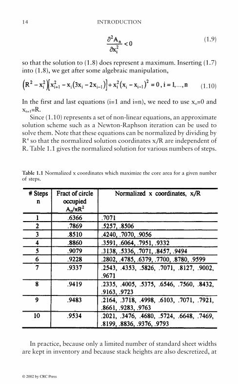
Since (1.10) represents a set of non-linear equations, an approximatesolution scheme such as a Newton-Raphson iteration can be used tosolve them. Note that these equations can be normalized by dividing byR4 so that the normalized solution coordinates xi/R are independent ofR. Table 1.1 gives the normalized solution for various numbers of steps.
Table 1.1 Normalized x coordinates which maximize the core area for a given numberof steps.
In practice, because only a limited number of standard sheet widthsare kept in inventory and because stack heights are also descretized, at
© 2002 by CRC Press
INTRODUCTION 15
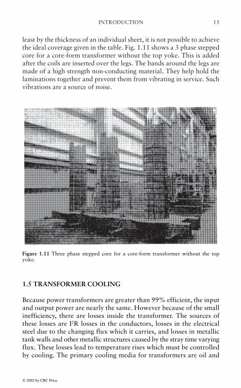
least by the thickness of an individual sheet, it is not possible to achievethe ideal coverage given in the table. Fig. 1.11 shows a 3 phase steppedcore for a core-form transformer without the top yoke. This is addedafter the coils are inserted over the legs. The bands around the legs aremade of a high strength non-conducting material. They help hold thelaminations together and prevent them from vibrating in service. Suchvibrations are a source of noise.
1.5 TRANSFORMER COOLING
Because power transformers are greater than 99% efficient, the inputand output power are nearly the same. However because of the smallinefficiency, there are losses inside the transformer. The sources ofthese losses are I2R losses in the conductors, losses in the electricalsteel due to the changing flux which it carries, and losses in metallictank walls and other metallic structures caused by the stray time varyingflux. These losses lead to temperature rises which must be controlledby cooling. The primary cooling media for transformers are oil and
Figure 1.11 Three phase stepped core for a core-form transformer without the topyoke.
© 2002 by CRC Press

INTRODUCTION16
air. In oil cooled transformers, the coils and core are immersed in anoil filled tank. The oil is then circulated through radiators or othertypes of heat exchanger so that the ultimate cooling medium is thesurrounding air or possibly water for some types of heat exchangers.In small distribution transformers, the tank surface in contact with theair provides enough cooling surface so that radiators are not needed.Sometimes in these units the tank surface area is augmented by meansof fins or corrugations.
The cooling medium in contact with the coils and core must provideadequate dielectric strength to prevent electrical breakdown ordischarge between components at different voltage levels. For thisreason, oil immersion is common in higher voltage transformers sinceoil has a higher breakdown strength than air. Often one can rely on thenatural convection of oil through the windings, driven by buoyancyeffects, to provide adequate cooling so that pumping isn’t necessary. Airis a more efficient cooling medium when it is blown by means of fansthrough the windings for air cooled units.
In some applications, the choice of oil or air is dictated by safetyconsiderations such as the possibility of fires. For units inside buildings,air cooling is common because of the reduced fire hazard. Whiletransformer oil is combustible, there is usually little danger of fire sincethe transformer tank is often sealed from the outside air or the oilsurface is blanketed with an inert gas such as nitrogen. Although theflash point of oil is quite high, if excessive heating or sparking occursinside an oil filled tank, combustible gasses could be released.
Another consideration in the choice of cooling is the weight of thetransformer. For mobile transformers such as those used on planes ortrains or units designed to be transportable for emergency use, aircooling might be preferred since oil adds considerably to the overallweight. For units not so restricted, oil is the preferred cooling mediumso that one finds oil cooled transformers in general use from largegenerator or substation units to distribution units on telephone poles.
There are other cooling media which find limited use in certainapplications. Among these is sulfur hexaflouride gas, usuallypressurized. This is a relatively inert gas which has a higher breakdownstrength than air and finds use in high voltage units where oil is ruledout for reasons such as those mentioned above and where air doesn’tprovide enough dielectric strength. Usually when referring to oil cooledtransformers, one means that the oil is standard transformer oil.However there are other types of oil which find specialized usage. Oneof these is silicone oil. This can be used at a higher temperature thanstandard transformer oil and at a reduced fire hazard.
© 2002 by CRC Press

INTRODUCTION 17
1.6 WINDING TYPES
For core-form power transformers, there are two main methods ofwinding the coils. These are sketched in Fig. 1.12. Both types arecylindrical coils, having an overall rectangular cross-section. In a diskcoil, the turns are arranged in horizontal layers called disks which arewound alternately out-in, in-out, etc. The winding is usually continuousso that the last inner or outer turn gradually transitions between theadjacent layers. When the disks have only one turn, the winding iscalled a helical winding. The total number of turns will usually dictatewhether the winding will be a disk or helical winding. The turns withina disk are usually touching so that a double layer of insulation separatesthe metallic conductors. The space between the disks is left open, exceptfor structural separators called key spacers. This allows room forcooling fluid to flow between the disks, in addition to providingclearance for withstanding the voltage difference between them.
Figure 1.12 Two major types of coil construction for core-form power transformers
© 2002 by CRC Press

INTRODUCTION18
In a layer coil, the coils are wound in vertical layers, top-bottom,bottom-top, etc. The turns are typically wound in contact with eachother in the layers but the layers are separated by means of spacers sothat cooling fluid can flow between them. These coils are also usuallycontinuous with the last bottom or top turn transitioning between thelayers.
Both types of winding are used in practice. Each type has itsproponents. In certain applications, one or the other type may be moreefficient. However, in general they can both be designed to functionwell in terms of ease of cooling, ability to withstand high voltagesurges, and mechanical strength under short circuit conditions.
If these coils are wound with more than one wire or cable in parallel,then it is necessary to insert cross-overs or transpositions which interchangethe positions of the parallel cables at various points along the winding.This is done to cancel loop voltages induced by the stray flux. Otherwisesuch voltages would drive currents around the loops formed when theparallel turns are joined at either end of the winding, creating extra losses.
The stray flux also causes localized eddy currents in the conductingwire whose magnitude depends on the wire cross-sectional dimensions,These eddy currents and their associated losses can be reduced bysubdividing the wire into strands of smaller cross-sectional dimensions.However these strands are then in parallel and must therefore betransposed to reduce the loop voltages and currents. This can be doneduring the winding process when the parallel strands are woundindividually. Wire of this type, consisting of individual strands coveredwith an insulating paper wrap, is called magnet wire. Thetranspositions can also be built into the cable. This is calledcontinuously transposed cable and generally consists of a bundle of 5–83 strands, each covered with a thin enamel coating. One strand at atime is transposed along the cable every 12 to 16 times its width so thatall the strands are eventually transposed approximately every 25–50cm (10–20 in) along the length of the cable. The overall bundle is thensheathed in a paper wrap.
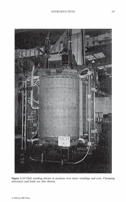
Fig. 1.13 shows a disk winding situated over inner windings and coreand clamped at either end via the insulating blocks and steel structureshown. Leads emerging from the top and bottom of one of the innerwindings are also visible on the right. The staggered short horizontalgaps shown are transition points between disks. Vertical columns of keyspacer projections are also barely visible. This outer high voltagewinding is center fed so that the top and bottom halves are connected inparallel. The leads feeding this winding are on the left.
© 2002 by CRC Press
INTRODUCTION 19
Figure 1.13 Disk winding shown in position over inner windings and core. Clampingstructures and leads are also shown.
© 2002 by CRC Press

INTRODUCTION20
1.7 INSULATION STRUCTURES
Transformer windings and leads must operate at high voltages relativeto the core, tank, and structural elements. In addition, different windingsand even parts of the same winding operate at different voltages. Thisrequires that some form of insulation between these various parts beprovided to prevent voltage breakdown or corona discharges. Thesurrounding oil or air which provides cooling has some insulatingvalue. The oil is of a special composition and must be purified toremove small particles and moisture. The type of oil most commonlyused, as mentioned previously, is called transformer oil. Furtherinsulation is provided by paper covering over the wire or cables. Whensaturated with oil, this paper has a high insulation value. Other typesof wire covering besides paper are sometimes used, mainly for specialtyapplications. Other insulating structures which are generally presentin sheet form, often wrapped into a cylindrical shape, are made ofpressboard. This is a material made of cellulose fibers which arecompacted together into a fairly dense and rigid matrix. Key spacers,blocking material, and lead support structures are also commonly madeof pressboard.
Although normal operating voltages are quite high, 10–500 kV, thetransformer must be designed to withstand even higher voltages which canoccur when lightning strikes the electrical system or when power issuddenly switched on or off in some part of the system. Howeverinfrequently these occur, they could permanently damage the insulation,disabling the unit, unless the insulation is designed to withstand them.Usually such events are of short duration. There is a time dependence tohow the insulation breaks down. A combination of oil and pressboardbarriers can withstand higher voltages for shorter periods of time. In otherwords, a short duration high voltage pulse is no more likely to causebreakdown than a long duration low voltage pulse. This means that thesame insulation that can withstand normal operating voltages which arecontinuously present can also withstand the high voltages arising fromlightning strikes or switching operations which are present only briefly. Inorder to insure that the abnormal voltages do not exceed the breakdownlimits determined by their expected durations, lightning or surge arrestersare used to limit them. These arresters thus guarantee that the voltages willnot rise above a certain value so that breakdown will not occur, assumingtheir durations remain within the expected range.
Because of the different dielectric constants of oil or air and paper,the electric stresses are unequally divided between them. Since the oil
© 2002 by CRC Press

INTRODUCTION 21
dielectric constant is about half that of paper and air is even a smallerfraction of papers’, the electric stresses are generally higher in oil orair than in the paper insulation. Unfortunately, oil or air has a lowerbreakdown stress than paper. In the case of oil, it has been found thatsubdividing the oil gaps by means of thin insulating barriers, usuallymade of pressboard, can raise the breakdown stress in the oil. Thuslarge oil gaps between the windings are usually subdivided by multiplepressboard barriers as shown schematically in Fig. 1.14. This isreferred to as the major insulation structure. The oil gap thicknessesare maintained by means of long vertical narrow sticks glued aroundthe circumference of the cylindrical pressboard barriers. Often thebarriers are extended by means of end collars which curve around theends of the windings to provide subdivided oil gaps at either end of thewindings to strengthen these end oil gaps against voltage breakdown.
Figure 1.14 Major insulation structure consisting of multiple barriers betweenwindings. Not all the keyspacers or sticks are shown.
The minor insulation structure consists of the smaller oil gapsseparating the disks and maintained by the key spacers which are narrowinsulators, usually made of pressboard, spaced radially around the disk’scircumference as shown in Fig. 1.14b. Generally these oil gaps are smallenough that subdivision is not required. In addition the turn to turninsulation, usually made of paper, can be considered as part of the minorinsulation structure. Fig. 1.15 shows a pair of windings as seen from the
© 2002 by CRC Press

INTRODUCTION22
top. The finger is pointing to the major insulation structure between thewindings. Key spacers and vertical sticks are also visible.
Figure 1.15 Top view of two windings showing the major insulation structure, keyspacers, and sticks
© 2002 by CRC Press

INTRODUCTION 23
The leads which connect the windings to the bushings or tapchangers or to other windings must also be properly insulated since theyare at high voltage and pass close to tank walls or structural supportswhich are grounded. They also can pass close to other leads at differentvoltages. High stresses can be developed at bends in the leads,particularly if they are sharp, so that additional insulation may berequired in these areas. Fig. 1.16 shows a rather extensive set of leadsalong with structural supports made of pressboard. The leads pass closeto the metallic clamps at the top and bottom and will also be near thetank wall when the core and coil assembly is inserted into the tank.
Figure 1.16 Leads and their supporting structure emerging from the coils on one sideof a 3 phase transformer
Although voltage breakdown levels in oil can be increased by meansof barrier subdivisions, there is another breakdown process which mustbe guarded against. This is breakdown due to creep. It occurs along thesurfaces of the insulation. It requires sufficiently high electric stressesdirected along the surface as well as sufficiently long uninterruptedpaths over which the high stresses are present. Thus the barriersthemselves, sticks, key spacers, and lead supports can be a source ofbreakdown due to creep. Ideally one should position these insulation
© 2002 by CRC Press

INTRODUCTION24
structures so that their surfaces conform to voltage equipotentialsurfaces to which the electric field is perpendicular. Thus there would beno electric fields directed along the surface. In practice, this is notalways possible so that a compromise must be reached.
The major and minor insulation designs, including overall windingto winding separation and number of barriers as well as disk to diskseparation and paper covering thickness, are often determined bydesign rules based on extensive experience. However, in cases of neweror unusual designs, it is often desirable to do a field calculation using afinite-element program or other numerical procedure. This can beespecially helpful when the potential for creep breakdown exists.Although these methods can provide accurate calculations of electricstresses, the breakdown process is not as well understood so that there isusually some judgment involved in deciding what level of electricalstress is acceptable.
1.8 STRUCTURAL ELEMENTS
Under normal operating conditions, the electromagnetic forces actingon the transformer windings are quite modest. However, if a shortcircuit fault occurs, the winding currents can increase 10–30 fold,resulting in forces of 100–900 times normal since the forces increaseas the square of the current. The windings and supporting structuremust be designed to withstand these fault current forces withoutpermanent distortion of the windings or supports. Because currentprotection devices are usually installed, the fault currents are interruptedafter a few cycles.
Faults can be caused by falling trees which hit power lines, providinga direct current path to ground or by animals or birds bridging acrosstwo lines belonging to different phases, causing a line to line short.These should be rare occurrences but over the 20–50 year lifetime of atransformer, their probability increases so that sufficient mechanicalstrength to withstand these is required.
The coils are generally supported at the ends with pressure rings.These are thick rings of pressboard or other material which cover thewinding ends. The center opening allows the core to pass through. Therings are in the range of 3–10 cm (1–4 in) for large power transformers.Some blocking made of pressboard or wood is required between thetops of the windings and the rings since all of the windings are not of thesame height. Additional blocking is usually placed between the ring
© 2002 by CRC Press
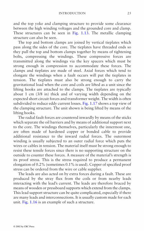
INTRODUCTION 25
and the top yoke and clamping structure to provide some clearancebetween the high winding voltages and the grounded core and clamp.These structures can be seen in Fig. 1.13. The metallic clampingstructure can also be seen.
The top and bottom clamps are joined by vertical tieplates whichpass along the sides of the core. The tieplates have threaded ends sothey pull the top and bottom clamps together by means of tighteningbolts, compressing the windings. These compressive forces aretransmitted along the windings via the key spacers which must bestrong enough in compression to accommodate these forces. Theclamps and tieplates are made of steel. Axial forces which tend toelongate the windings when a fault occurs will put the tieplates intension. The tieplates must also be strong enough to carry thegravitational load when the core and coils are lifted as a unit since thelifting hooks are attached to the clamps. The tieplates are typicallyabout 1 cm (3/8 in) thick and of varying width depending on theexpected short circuit forces and transformer weight. The width is oftensubdivided to reduce eddy current losses. Fig. 1.17 shows a top view ofthe clamping structure. The unit shown is being lifted by means of thelifting hooks.
The radial fault forces are countered inwardly by means of the stickswhich separate the oil barriers and by means of additional support nextto the core. The windings themselves, particularly the innermost one,are often made of hardened copper or bonded cable to provideadditional resistance to the inward radial forces. The outermostwinding is usually subjected to an outer radial force which puts thewires or cables in tension. The material itself must be strong enough toresist these tensile forces since there is no supporting structure on theoutside to counter these forces. A measure of the material’s strength isits proof stress. This is the stress required to produce a permanentelongation of 0.2% (sometimes 0.1% is used). Copper of specified proofstress can be ordered from the wire or cable supplier.
The leads are also acted on by extra forces during a fault. These areproduced by the stray flux from the coils or from nearby leadsinteracting with the lead’s current. The leads are therefore braced bymeans of wooden or pressboard supports which extend from the clamps.This lead support structure can be quite complicated, especially if thereare many leads and interconnections. It is usually custom made for eachunit. Fig. 1.16 is an example of such a structure.
© 2002 by CRC Press

INTRODUCTION26
Figure 1.17 Top view of clamping stmcture for a 3 phase transformer.
© 2002 by CRC Press
INTRODUCTION 27
The assembled coil, core, clamps, and lead structure is placed in atransformer tank. The tank serves many functions, one of which is tocontain the oil for an oil filled unit. It also provides protection not onlyfor the coils and other transformer structures but for personnel from thehigh voltages present. If made of soft (magnetic) steel, it keeps stray fluxfrom getting outside the tank. The tank is usually made airtight so thatair doesn’t enter and oxidize the oil.
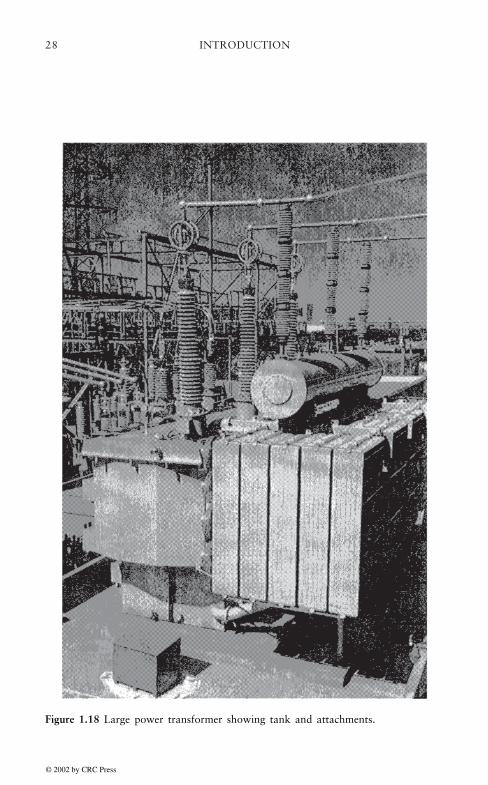
Aside from being a containment vessel, the tank also has numerousattachments such as bushings for getting the electrical power into andout of the unit, an electronic control and monitoring cabinet forrecording and transferring sensor information to remote processors andreceiving control signals, and radiators with or without fans to providecooling. On certain units, there is a separate tank compartment for tapchanging equipment. Also some units have a conservator attached tothe tank cover or to the top of the radiators. This is a large, usuallycylindrical, structure which contains oil in communication with themain tank oil. It also has an air space which is separated from the oil bya sealed diaphragm. Thus, as the tank oil expands and contracts due totemperature changes, the flexible diaphragm accommodates thesevolume changes while maintaining a sealed oil environment. Fig 18shows a large power transformer installed in a switchyard. Thecylindrical conservator is visible on top of the radiator bank. The highand low voltage bushings which are mounted on the tank cover arevisible. Also shown are the surge arresters which in this case aremounted on top of the conservator.
© 2002 by CRC Press
INTRODUCTION28
Figure 1.18 Large power transformer showing tank and attachments.
© 2002 by CRC Press

INTRODUCTION 29
1.9 THREE PHASE CONNECTIONS
There are two basic types of 3 phase connections in common use, the Y(Wye) and ∆ (Delta) connections as illustrated schematically in Fig.1.19. In the Y connection, all 3 phases are connected to a common pointwhich may or may not be grounded. In the ∆ connection, the phases areconnected end to end with each other. In the Y connection, the linecurrent flows directly into the winding where it is called the winding orphase current. Note that in a balanced 3 phase system, the currents sumto zero at the common node in Fig. 1.19a. Therefore, under balancedconditions, even if this point were grounded, no current would flow toground. In the ∆ connection, the line and phase currents are different.On the other hand, the line to line voltages in the Y connection differfrom the voltages across the windings or phase voltages whereas theyare the same in the ∆ connection. Note that the coils are shown atangles to each other in the figure to emphasize the type of interconnectionwhereas in practice they are side by side and vertically oriented asshown for example in Fig. 1.16. The leads are snaked about to handlethe interconnections.
Figure 1.19 Basic 3 phase connections
© 2002 by CRC Press

INTRODUCTION30
To be more quantitative about the relationship between line andphase quantities, we must resort to phasor notation. The 3 phasevoltages as shown in Fig. 1.5 can be written
Va=Vo cos(ωt), Vb=Vo cos(ωt+240°), Vc=Vo cos(ωt+120°) (1.11)
where Vo is the peak voltage, t is the time, and ω the angular frequency(ω=2πf, f the frequency in Hz). Actually the 240° and 120° above shouldbe expressed in radians to be consistent with the expression for ω. Whenusing degrees, ω=360°f should be understood. Using the identity
ejθ=cosθ+jsinθ (1.12)
where j is the imaginary unit (j2=”1), (1.11) 10 can be written
(1.13)
where Re denotes taking the real part of.Complex quantities are more easily visualized as vectors in the
complex plane. Thus (1.12) can be described as a vector of unitmagnitude in the complex plane with real component cos θ andimaginary component sin θ This can be visualized as a unit vectorstarting at the origin and making an angle θ with the real axis. Anycomplex number can be described as such a vector but having, ingeneral, a magnitude different from unity. Fig. 1.20 shows this pictorialdescription. As θ increases, the vector rotates in a counter clockwisefashion about the origin. If we let θ=ωt, then as time increases, thevector rotates with a uniform angular velocity ω about the origin. Whendealing with complex numbers having the same time dependence, ejωt,as in (1.13), it is customary to drop this term or to simply set t=0. Sincethese vectors all rotate with the same angular velocity, their relativepositions with respect to each other in the complex plane remainunchanged, i.e. if the angle between two such vectors is 120° at t=0, itwill remain 120° for all subsequent times. The resulting vectors, withcommon time dependence removed, are called phasors.
© 2002 by CRC Press

INTRODUCTION 31
Using bold faced type to denote phasors, from (1.13) define
(1.14)
Then to recover (1.13), multiply by the complex time dependence andtake the real part. These phasors are also shown in Fig. 1.20. Note thatthe process of recovering (1.13), which is equivalent to (1.11), can bevisualized as multiplying by the complex time dependence and takingtheir projections on the real axis as the phasors rotate counterclockwisewhile maintaining their relative orientations. Thus Va peaks (has maximumpositive value) at t=0, Vb achieves its positive peak value next at ωt=120°followed by Vc at ωt=240°. This ordering is called positive sequenceordering and Va, Vb, Vc are referred to as a positive sequence set of voltages.A similar set of phasors can also be used to describe the currents. Notethat, using vector addition, this set of phasors adds to zero as is evident inFig. 1.20.
If Va, Vb, Vc are the phase voltages in a Y connected set oftransformer windings, let Vab denote the line to line voltage between
Figure 1.20 Phasors as vectors in the complex plane
© 2002 by CRC Press

INTRODUCTION32
phases a and b, etc, for the other line to line voltages. Then thesevoltages are given by,
(1.15)
Using a phasor description, these can be readily calculated. The line toline phasors are shown graphically in Fig. 1.21. Fig. 1.21a shows thevector subtraction process explicitly and Fig. 1.21b shows the set of 3line to line voltage phasors. Note that these form a positive sequence setthat is rotated 30° relative to the phase voltages. The line to line voltagemagnitude can be found geometrically as the diagonal of theparallelogram formed by equal length sides making an angle of 120°with each other. Thus we have
(1.16)
where | | denotes taking the magnitude. We have used the fact that thedifferent phase voltages have the same magnitude.
Figure 1.21 Phasor representation of line to line voltages and their relation to thephase voltages in a Y connected set of 3 phase windings
© 2002 by CRC Press

INTRODUCTION 33
Thus the magnitude of the line to line voltage is √3 times the phasevoltage magnitude in Y connected transformer coils. Since the phasevoltages are internal to the transformer and therefore impact thewinding insulation structure, a more economical design is possible ifthese can be lowered. Hence, a Y connection is often used for the highvoltage coils of a 3 phase transformer.
The relationship between the phase and line currents of a deltaconnected set of windings can be found similarly. From Fig. 1.19, wesee that the line currents are given in terms of the phase currents by
(1.17)
These are illustrated graphically in Fig. 1.22. Note that, as shown inFig. 1.22b, the line currents form a positive sequence set rotated -30°relative to the phase currents. One could also say that the phase currentsare rotated +30° relative to the line currents. The magnitude relationshipbetween the phase and line currents follows similarly as for the voltagesin a Y connection. However, let us use phasor subtraction directly in(1.17) to show this. We have
(1.18)
where we have used |Iab|=|Ica|.
© 2002 by CRC Press

INTRODUCTION34
Thus the magnitude of the line current into or out of a delta connectedset of windings are times the winding or phase current magnitude.Since low voltage windings have higher phase currents than high voltagewindings, it is common to connect these in delta because lowering thephase currents can produce a more economical design.
The rated power into a phase of a 3 phase transformer is the terminalvoltage to ground times the line current. We can deal with magnitudesonly here since rated power is at unity power factor. Thus for a Yconnected set of windings, the terminal voltage to ground equals thevoltage across the winding and the line current equals the phasecurrent. Hence the total rated power into all three phases is 3×the phasevoltage ×the phase current which is the total winding power. In terms ofthe line to line voltages and line current, we have, using (1.16), that thetotal rated power is × the line to line voltage×the line current.
For a delta connected set of windings, there is considered to be avirtual ground at the center of the delta. From the geometricalrelationships we have developed above, the line voltage to ground istherefore the line to line voltage÷ . Thus the total rated power is 3×the line voltage to ground×the line current= ×line to line voltage×theline current. Since the phase voltage equals the line to line voltage andthe phase current=1/ × the line current according to (1.18), the totalrated power can also be expressed as 3×the phase voltage×the phasecurrent or the total winding power. Thus the total rated power, whether
Figure 1.22 Phaser representation of line currents and their relation to the phasecurrents in a delta connected set of 3 phase windings
© 2002 by CRC Press

INTRODUCTION 35
expressed in terms of line quantities or phase quantities, is the same forY and delta connected windings. We also note that the rated inputpower is the same as the power flowing through the windings. This maybe obvious here, but there are some connections where this is not thecase, in particular autotransformer connections.
An interesting 3 phase connection is the open delta connection. Inthis connection, one of the windings of the delta is missing although theterminal connections remain the same. This is illustrated in Fig. 1.23.This could be used especially if the 3 phases consist of separate unitsand if one of the phases is missing either because it is intended for futureexpansion or it has been disabled for some reason. Thus instead of(1.17) for the relationship between line and phase currents, we have
(1.19)
But this implies
Ia+Ib+Ic=0 (1.20)
so that the terminal currents form a balanced 3 phase system. Likewisethe terminal voltages form a balanced 3 phase system. However only 2phases are present in the windings. As far as the external electricalsystem is concerned, the 3 phases are balanced. The total rated input oroutput power is, as before, 3×line voltage to ground×line current= ×lineto line voltage×line current. But as (1.19) shows, the line current has thesame magnitude as the phase or winding current. Also, as before, theline to line voltage equals the voltage across the winding or phasevoltage. Hence the total rated power is ×phase voltage×phase current.Previously for a full delta connection, we found that the total ratedpower was 3×phase voltage×phase current. Thus for the open delta, therated power is only 1/ =0.577 times that of a full delta connection. Asfar as winding utilization goes, in the full delta connection 2 windingscarry 2/3×3×phase voltage×phase current=2×phase voltage×phasecurrent. Thus the winding power utilization in the open delta connectionis /2=0.866 times that of a full delta connection. Thus this connectionis not as efficient as a full delta connection.
© 2002 by CRC Press

INTRODUCTION36
1.10 MODERN TRENDS
Changes in power transformers tend to occur very slowly. Issues ofreliability over long periods of time and compatibility with existingsystems must be addressed by any new technology. A major changewhich has been ongoing since the earliest transformers is the improvementin core steel. The magnetic properties, including losses, have improveddramatically over the years. Better stacking methods, such as steppedlapped construction, have resulted in lower losses at the joints. The useof laser or mechanical scribing has also helped lower the losses in thesesteels. Further incremental improvements in all of these areas can beexpected.
The development of amorphous metals as a core material isrelatively new. Although these materials have very low losses, lowerthan the best rolled electrical steels, they also have a rather lowsaturation induction (~1.5 Tesla versus 2.1 Tesla for rolled steels). Theyare also rather brittle and difficult to stack. This material has tended tobe more expensive than rolled electrical steel and, since expense is
Figure 1.23 Open delta connection
© 2002 by CRC Press
INTRODUCTION 37
always an issue, has limited their use. However, this could change withthe cost of no-load losses to the utilities. Amorphous metals have founduse as wound cores in distribution transformers. However, their use asstacked cores in large power transformers is problematic.
The development of improved wire types, such as transposed cablewith epoxy bonding, is an ongoing process. Newer types of wireinsulation covering such as Nomex are being developed. Nomex is asynthetic material which can be used at higher temperatures than paper,It also has a lower dielectric constant than paper so it produces a morefavorable stress level in the adjacent oil than paper. Although it ispresently a more expensive material than paper, it has found a niche inair cooled transformers or in the rewinding of older transformers. Itsthermal characteristics would probably be underutilized in transformeroil filled transformers because of the limitations on the oil temperatures.
Pressboard insulation has undergone improvements over time suchas precompressing to produce higher density material which results ingreater dimensional stability in transformer applications. This isespecially helpful in the case of key spacers which bear thecompressional forces acting on the winding. Also pre-formed partsmade of pressboard, such as collars at the winding ends and highvoltage lead insulation assemblies, are becoming more common andare facilitating the development of higher voltage transformers.
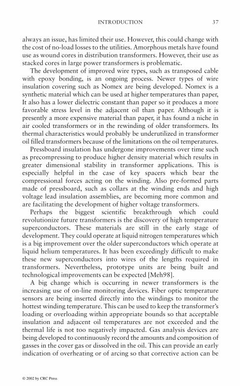
Perhaps the biggest scientific breakthrough which couldrevolutionize future transformers is the discovery of high temperaturesuperconductors. These materials are still in the early stage ofdevelopment. They could operate at liquid nitrogen temperatures whichis a big improvement over the older superconductors which operate atliquid helium temperatures. It has been exceedingly difficult to makethese new superconductors into wires of the lengths required intransformers. Nevertheless, prototype units are being built andtechnological improvements can be expected [Meh98].
A big change which is occurring in newer transformers is theincreasing use of on-line monitoring devices. Fiber optic temperaturesensors are being inserted directly into the windings to monitor thehottest winding temperature. This can be used to keep the transformer’sloading or overloading within appropriate bounds so that acceptableinsulation and adjacent oil temperatures are not exceeded and thethermal life is not too negatively impacted. Gas analysis devices arebeing developed to continuously record the amounts and composition ofgasses in the cover gas or dissolved in the oil. This can provide an earlyindication of overheating or of arcing so that corrective action can be
© 2002 by CRC Press

INTRODUCTION38
taken before the situation deteriorates too far. Newer fiber optic currentsensors based on the Faraday effect are being developed. These weighconsiderably less than present current sensors and are much less bulky.Newer miniaturized voltage sensors are also being developed. Sensordata in digitized form can be sent from the transformer to a remotecomputer for further processing. Newer software analysis tools shouldhelp to more accurately analyze fault conditions or operationalirregularities.
Although tap changers are mechanical marvels which operate veryreliably over hundreds of thousands of tap changing operations, as withany mechanical device, they are subject to wear and must be replacedor refurbished from time to time. Electronic tap changers, using solidstate components, have been developed. Aside from essentiallyeliminating the wear problem, they also have a much faster responsetime than mechanical tap changers which could be very useful in someapplications. Their expense relative to mechanical tap changers hasbeen one factor limiting their use. Further developments perhapsresulting in lower cost can be expected in this area.
As mentioned previously, there are incentives to transmit power athigher voltages. Some of the newer high voltage transmission linesoperate in a d.c. mode. In this case, the conversion equipment at theends of the line which change a.c. to d.c. and vice versa requires atransformer. However this transformer does not need to operate at theline voltage. For high voltage a.c. lines, however, the transformer mustoperate at these higher voltages. At present, transformers which operatein the range of 750–800 kV have been built. Even higher voltage unitshave been developed, but this technology is still somewhatexperimental. A better understanding of high voltage breakdownmechanisms, especially in oil, is needed to spur growth in this area.
© 2002 by CRC Press

39
2. TRANSFORMER CIRCUIT MODELS,INCLUDING MAGNETIC CORE
CHARACTERISTICS, ANDAPPLICATIONS
Summary The characteristics of transformer cores are discussed interms of their basic magnetic properties and how these influencetransformer design. Special emphasis is placed on silicon steel coressince these are primarily used in power transformers. However, themagnetic concepts discussed are applicable to all types of cores. Themagnetic circuit approximation is introduced and its use in obtainingthe properties of cores with joints or gaps is discussed. Basic featuresof the magnetization process are used to explain inrush current andto calculate its magnitude. The inclusion of the transformer core inelectrical circuit models is discussed. Although non-linearities in themagnetic characteristics can be included in these models, for inductionswell below saturation a linear approximation is adequate. For manypurposes, the circuit models can be further approximated byeliminating the core. As an application, an approximate circuit modelis used to calculate the voltage regulation of a two windingtransformer.
2.1 INTRODUCTION
Transformer cores are constructed predominantly of ferromagnetic material.The most common material used is iron, with the addition of small amountsof silicon and other elements which help improve the magnetic propertiesand/or lower losses. Other materials which find use in electronic transformersare the nickel-iron alloys (permalloys) and the iron-oxides (ferrites). Theamorphous metals, generally consisting of iron, boron, and other additions,are also finding use as cores for distribution transformers. These materialsare all broadly classified as ferromagnetic and, as such, share many propertiesin common. Among these are saturation magnetization or induction,hysteresis, and a Curie temperature above which they cease to beferromagnetic.
© 2002 by CRC Press
TRANSFORMER CIRCUIT MODELS40
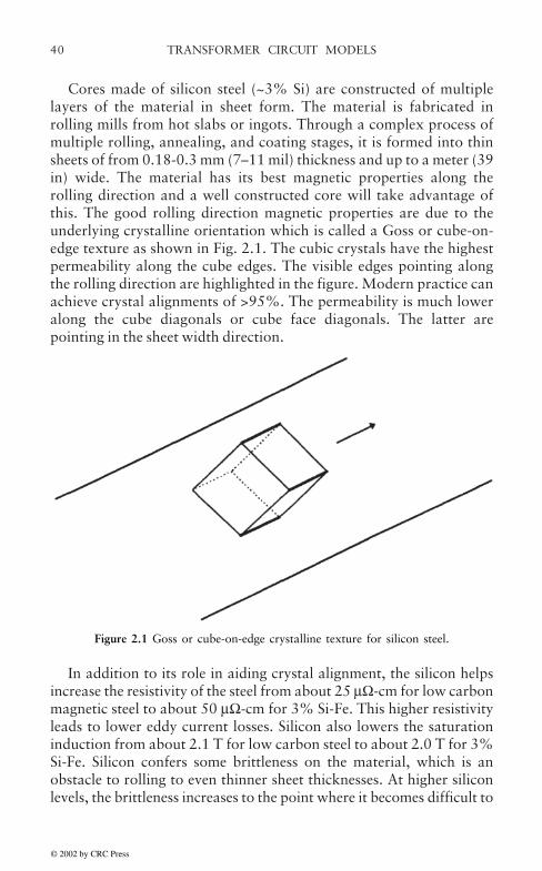
Cores made of silicon steel (~3% Si) are constructed of multiplelayers of the material in sheet form. The material is fabricated inrolling mills from hot slabs or ingots. Through a complex process ofmultiple rolling, annealing, and coating stages, it is formed into thinsheets of from 0.18-0.3 mm (7–11 mil) thickness and up to a meter (39in) wide. The material has its best magnetic properties along therolling direction and a well constructed core will take advantage ofthis. The good rolling direction magnetic properties are due to theunderlying crystalline orientation which is called a Goss or cube-on-edge texture as shown in Fig. 2.1. The cubic crystals have the highestpermeability along the cube edges. The visible edges pointing alongthe rolling direction are highlighted in the figure. Modern practice canachieve crystal alignments of >95%. The permeability is much loweralong the cube diagonals or cube face diagonals. The latter arepointing in the sheet width direction.
Figure 2.1 Goss or cube-on-edge crystalline texture for silicon steel.
In addition to its role in aiding crystal alignment, the silicon helpsincrease the resistivity of the steel from about 25 µΩ-cm for low carbonmagnetic steel to about 50 µΩ-cm for 3% Si-Fe. This higher resistivityleads to lower eddy current losses. Silicon also lowers the saturationinduction from about 2.1 T for low carbon steel to about 2.0 T for 3%Si-Fe. Silicon confers some brittleness on the material, which is anobstacle to rolling to even thinner sheet thicknesses. At higher siliconlevels, the brittleness increases to the point where it becomes difficult to
© 2002 by CRC Press

TRANSFORMER CIRCUIT MODELS 41
roll. This is unfortunate because at 6% silicon content, themagnetostriction of the steel disappears. Magnetostriction is a lengthchange or strain which is produced by the induction in the material.This contributes to the noise level in a transformer.
The nickel-iron alloys or permalloys are also produced in sheetform. Because of their malleability, they can be rolled extremely thin.The sheet thinness results in very low eddy current losses so that thesematerials find use in high frequency applications. Their saturationinduction is lower than that for silicon steel.
Ferrite cores are made of sintered power. They generally haveisotropic magnetic properties. They can be cast directly into the desiredshape or machined after casting. They have extremely high resistivitieswhich permits their use in high frequency applications. However, theyhave rather low saturation inductions.
Amorphous metals are produced by directly casting the liquid meltonto a rotating, internally cooled, drum. The liquid solidifies extremelyrapidly, resulting in the amorphous (non-crystalline) texture of the finalproduct. The material comes off the drum in the form of a thin ribbonwith controlled widths which can be as high as ~25 cm (10 in). Thematerial has a magnetic anisotropy determined by the casting directionand subsequent magnetic anneals so that the best magnetic propertiesare along the casting direction. Their saturation induction is about 1.5T. Because of their thinness and composition, they have extremely lowlosses. These materials are very brittle which has limited their use towound cores. Their low losses make them attractive for use indistribution transformers, especially when no-load loss evaluations arehigh.
Ideally a transformer core would carry the flux along a direction ofhighest permeability and in a closed path. Path interruptions caused byjoints, which are occupied by low permeability air or oil, lead to pooreroverall magnetic properties. In addition, the cutting or slittingoperations can introduce localized stresses which degrade the magneticproperties. In stacked cores, the joints are often formed by overlappingthe laminations in steps to facilitate flux transfer across the joint.Nevertheless, the corners result in regions of higher loss. This can beaccounted for in design by multiplying the ideal magnetic circuit losses,usually provided by the manufacturer on a per unit weight basis, by abuilding factor >1. Another, possibly better, way to account for theextra loss is to apply a loss multiplying factor to the steel occupying thecorner or joint region only. More fundamental methods to account forthese extra losses have been proposed but these tend to be too elaborate
© 2002 by CRC Press

TRANSFORMER CIRCUIT MODELS42
for routine use. Joints also give rise to higher exciting current, i.e. thecurrent in the coils necessary to drive the required flux around the core.
2.2 BASIC MAGNETISM
The discovery by Oersted that currents give rise to magnetic fields ledAmpere to propose that material magnetism results from localizedcurrents. He proposed that large numbers of small current loops,appropriately oriented, could create the magnetic fields associated withmagnetic materials and permanent magnets. At the time, the atomicnature of matter was not understood. With the Bohr model of the atom,where electrons are in orbit around a small massive nucleus, the localizedcurrents could be associated with the moving electron. This gives rise toan orbital magnetic moment which persists even though a quantumdescription has replaced the Bohr model. In addition to the orbitalmagnetism, the electron itself was found to possess a magnetic momentwhich cannot be understood simply from the circulating current point ofview. Atomic magnetism results from a combination of both orbital andelectron moments.
In some materials, the atomic magnetic moments either cancel or arevery small so that little material magnetism results. These are known asparamagnetic or diamagnetic materials, depending on whether an appliedfield increases or decreases the magnetization. Their permeabilitiesrelative to vacuum are nearly equal to 1. In other materials, the atomicmoments are large and there is an innate tendency for them to align due toquantum mechanical forces. These are the ferromagnetic materials. Thealignment forces are very short range, operating only over atomicdistances. Nevertheless, they create regions of aligned magnetic moments,called domains, within a magnetic material. Although each domain has acommon orientation, this orientation differs from domain to domain. Thenarrow separations between domains are regions where the magneticmoments are transitioning from one orientation to another. Thesetransition zones are referred to as domain walls.
In non-oriented magnetic materials, the domains are typically verysmall and randomly oriented. With the application of a magnetic field,the domain orientation tends to align with the field direction. Inaddition, favorably orientated domains tend to grow at the expense ofunfavorably oriented ones. As the magnetic field increases, the domainseventually all point in the direction of the magnetic field, resulting in astate of magnetic saturation. Further increases in the field cannot orient
© 2002 by CRC Press

TRANSFORMER CIRCUIT MODELS 43
more domains so the magnetization does not increase but is said tosaturate. From this point on, further increases in induction are due toincreases in the field only.
The relation between induction, B, magnetization, M, and field, H,in SI units, is
B=µo(H+M) (2.1)
For many materials, M is proportional to H,
M=χH (2.2)
where χ is the susceptibility which need not be a constant. Substitutinginto (2.1)
B=µo(1+χ)H=µoµrH (2.3)
where µo=1+χ is the relative permeability. We see directly in (2.1) that,as M saturates because all the domains are similarly oriented, B canonly increase due to increases in H. This occurs at fairly high H orexciting current values, since H is proportional to the exciting current.At saturation, since all the domains have the same orientation, there areno domain walls. Since H is generally small compared to M for highpermeability ferromagnetic materials up to saturation, the saturationmagnetization and saturation induction are nearly the same and will beused interchangeably.
As the temperature increases, the thermal energy begins to competewith the alignment energy and the saturation magnetization begins tofall until the Curie point is reached where ferromagnetism completelydisappears. For 3 % Si-Fe, the saturation magnetization or induction at20 °C is 2.0 T and the Curie temperature is 746 °C. This should becompared with pure iron where the saturation induction at 20 °C is 2.1T and the Curie temperature is 770 °C. The fall off with temperaturefollows fairly closely a theoretical relationship between ratios ofsaturation induction at absolute temperature T to saturation inductionat T = 0 °K to the ratio of absolute temperature T to the Curietemperature expressed in °K. For pure iron, this relationship is showngraphed in Fig. 2.2 [Ame57]. This same graph also applies ratherclosely to other iron containing magnetic materials such as Si-Fe aswell as to nickel and cobalt based magnetic materials.
© 2002 by CRC Press

TRANSFORMER CIRCUIT MODELS44
Thus to find the saturation magnetization of 3 % Si-Fe at a temperatureof 200 °C=473 °K, take the ratio T/TC=0.464, From the graph, thiscorresponds to Ms/M0=0.94. On the other hand, we know that at 20 °Cwhere T/TC=0.287 that Ms/M0=0.98. Thus M0= 2.0/0.98=2.04. ThusMs(T=200 °C)=0.94(2.04)=1.92 T. This is only a 4 % drop in saturationmagnetization. Considering that core temperatures are unlikely to reach200 °C, temperature effects on magnetization should not be a problemin transformers under normal operating conditions.
Ferromagnetic materials typically exhibit the phenomenon ofmagnetostriction, i.e. a length change or strain resulting from theinduction or flux density which they carry. Since this length change isindependent of the sign of the induction, for an a.c. induction atfrequency f, the length oscillations occur at frequency 2f. These lengthvibrations contribute to the noise level in transformers.Magnetostriction is actually a fairly complex phenomenon and canexhibit hysteresis as well as anisotropy.
Figure 2.2 Relationship between saturation magnetization and absolute temperature,expressed in relative terms, for pure iron. This also applies reasonably well to otherferromagnetic materials containing predominately iron, nickel, or cobalt.
© 2002 by CRC Press

TRANSFORMER CIRCUIT MODELS 45
Another source of noise in transformers, often overlooked, resultsfrom the transverse vibrations of the laminations at unsupported freeends. This can occur at the outer surfaces of the core and shunts if theseare not constrained. This can be shown qualitatively by considering thesituation shown in Fig. 2.3. In Fig. 2.3a, we show a leakage flux densityvector B1 impinging on a packet of tank shunt laminations which areflat against the tank wall and rigidly constrained. After striking thelamination packet, the flux is diverted into the packet and transportedupward since we are looking at the bottom end. In Fig. 2.3b, the outerlamination is constrained only up to a certain distance from the end, d,beyond which it is free to move. We show its loose end at a distance xfrom the rest of the packet. Part of the flux density B1 is diverted alongthis outer packet and a reduced flux density B2 impinges on theremaining packets. We can assume the magnetic shunts are linear sincethe flux density they carry is usually far below saturation. Themagnetic energy for linear materials is given by
(2.4)
Using B=µoµτ H, this becomes
(2.5)
In highly oriented Si-Fe, µr is generally quite large (µr>5000) so thatmost of the magnetic energy resides in the oil or air where µr=1. Thuswe can ignore the energy stored in the laminations. For the situationshown in Fig. 2.3, let be a distance along which B1 is parallel andreasonably constant and let B1 also be constant through a cross-sectionalarea A determined by d and a unit distance into the paper. Then themagnetic energy associated with Fig. 2.3b is
(2.6)
The magnetic force component in the x direction is
(2.7)
© 2002 by CRC Press

TRANSFORMER CIRCUIT MODELS46
Since B2<B1, this force acts to pull the outer lamination outward inthe direction of x. It is independent of the sign of B so that if B issinusoidal of frequency f, Fm,x will have a frequency of 2f. Thus itcontributes to the transformer noise at the same frequency asmagnetostriction.
Figure 2.3 Geometry for simplified force calculation for a loose end lamination.
2.3 HYSTERESIS
Hysteresis, as the name implies, means that the present state of aferromagnetic material depends on its past magnetic history. This isusually illustrated by means of a B-H diagram. Magnetic field changesare assumed to occur slowly enough that eddy current effects can beignored. We assume the B and H fields are collinear although, ingeneral, they need not be. Thus we can drop the vector notation. If westart out with a completely demagnetized specimen (this state requirescareful preparation) and increase the magnetic field from 0, the materialwill follow the initial curve as shown in Fig. 2.4a. This curve can becontinued to saturation, B2. If at some point along the initial curve, the
© 2002 by CRC Press

TRANSFORMER CIRCUIT MODELS 47
field is reversed and decreased, the material will follow a normalhysteresis loop as shown in Fig. 2.4b. If the magnetic field is cycledrepeatedly between ±Hmax, the material will stay on a normal hysteresisloop determined by Hmax, their being a whole family of such loops asshown in Fig. 2.4c. The largest loop occurs when Bmax reaches Bs. Thisis called the major loop. These loops are symmetrical about the origin.If at some point along a normal loop, other than the extreme points,the field is reversed and cycled through a smaller cycle back to itsoriginal value before the reversal occurred, a minor or incrementalloop is traced as shown in Fig. 2.4d. Considering the many otherpossibilities for field reversals, the resulting hysteresis paths can becomequite complicated.
Figure 2.4 Hysteresis processes
© 2002 by CRC Press

TRANSFORMER CIRCUIT MODELS48
Perhaps the most important magnetic path is a normal hysteresisloop since this is traced in a sinusoidal cyclic magnetization process.Several key points along such a path are shown in Fig. 2.5. As the fieldis lowered from Hmax to zero, the induction remaining is called theremanence, Br. As the field is further lowered into negative territory, theabsolute value of the field at which the induction drops to zero is calledthe coercivity, Hc. Because the loop is symmetrical about the origin,there are corresponding points on the negative branches. At any pointon a magnetization path, the ratio of B to H is called the permeabilitywhile the slope of the B-H curve at that point is called the differentialpermeability. Other types of permeability can be defined. The area ofthe hysteresis loop is the magnetic energy per unit volume and per cycledissipated in hysteresis processes.
Figure 2.5 Key points along a normal hystersis loop
In oriented Si-Fe, the relative permeability for inductions reasonablybelow saturation is so high that the initial curve is close to the B axis ifB and H are measured in the same units as they are in the Gaussiansystem or if B vs µoH is plotted in the SI system. In addition, thehysteresis loops are very narrow in these systems of units and closelyhug the initial curve. Thus for all practical purposes, we can assume a
© 2002 by CRC Press

TRANSFORMER CIRCUIT MODELS 49
single valued B-H characteristic for these high permeability materialscoinciding with the initial curve. Since inductions in transformer coresare kept well below saturation in normal operation to avoid highexciting currents, the effects of saturation are hardly noticeable and thecore, for many purposes, can be assumed to have a constantpermeability.
2.4 MAGNETIC CIRCUITS
In stacked cores and especially in cores containing butt joints as wellas in gapped reactor cores, the magnetic path for the flux is not througha homogeneous magnetic material. Rather there are gaps occupied byair or oil or other non-magnetic materials of relative permeabilityequal to 1. In such cases, it is possible to derive effective permeabilitiesby using a magnetic circuit approximation. This approximation derivesfrom the mathematical similarity of magnetic and electrical laws. Inresistive electrical circuits, the conductivities of the wires and circuitelements are usually so much higher than the surrounding medium(usually air) that little current leaks away from the circuit. However,in magnetic circuits where the flux corresponds to the electric current,the circuit permeability, which is the analog of conductivity, is notorders of magnitude higher than that of the surrounding medium sothat flux leakage does occur. Thus, whereas the circuit approach isnearly exact for electric circuits, it is only approximate for magneticcircuits [Del94].
Corresponding to Kirchoff’s current law at a node
(2.8)
where Ii is the current into a node along a circuit branch i (positive ifentering the node, negative if leaving), we have the approximate magneticcounterpart
(2.9)
where Φi is the flux into a node. Whereas (2.8) is based on conservationof current and ultimately charge, (2.9) is based on conservation of flux.Kirchoff’s voltage law can be expressed
© 2002 by CRC Press

TRANSFORMER CIRCUIT MODELS50
(2.10)
where the voltage drops Vi are taken around the loop in which an emf isinduced. The electric field path integral in (2.10) is an alternate way ofexpressing the voltage drops. With E↔H, the magnetic analogy is
(2.11)
In this case, (2.11) is exact.In terms of the current density J and flux density B, we have
(2.12)
so that J and B are corresponding quantities in the two systems. Ohm’slaw in its basic form can be written
J=σE (2.13)
where σ is the conductivity. This corresponds to
B=µH (2.14)
in the magnetic system, where µ. is the permeability.To obtain resistance and corresponding reluctance expressions for
simple geometries, consider a resistive or reluctive element of length Land uniform cross-sectional area A as shown in Fig. 2.6. Let a uniformcurrent density J flow in the resistive element and a uniform flux densityB flow through the magnetic element. Then
(2.15)
Let a uniform electric field E drive the current and a uniform magneticfield H drive the flux. Then
(2.16)
Using (2.13), we have
© 2002 by CRC Press

TRANSFORMER CIRCUIT MODELS 51
(2.17)
where the quantity in parenthesis is recognized as the resistance. Similarlyfrom (2.14),
(2.18)
where the quantity in parenthesis is called the reluctance. A similaranalysis could be carried out for other geometries using the basic fieldcorrespondences.
As an application of the circuit approach, consider a simplemagnetic core with an air gap as shown in Fig. 2.7. A flux Φ is drivenaround the circuit by a coil generating an mmf of NI. The path throughthe magnetic core of permeability µ=µoµr has mean length L and thepath in the air gap of permeability µo has length Lo. The reluctances inthe magnetic material and air gap are
(2.19)
Since these reluctances are in series, we have
(2.20)
Figure 2.6 Geometries for simple resistance and reluctance calculation
© 2002 by CRC Press

TRANSFORMER CIRCUIT MODELS52
Thus since µr can be quite large, the reluctance with air gap can bemuch larger than that without so that more mmf is required to drive agiven flux. Note that we ignored fringing in the air gap. This could beapproximately accounted for by letting the area A be larger in the airgap than in the core material.
Figure 2.7 Air gap magnet driven by mmf=NI
In general, for two reluctances in series having the same cross-sectional area A but lengths L1, L2 and permeabilities µ1, µ2, the totalreluctance is
(2.21)
where L=L1+L2, f1=L1/L, f2=L2/L. Thus the effective permeability of thecombination is given by
(2.22)
This could be extended to more elements in series. An identicalrelationship holds for the effective conductivity of a series of equal cross-sectional area resistive elements.
© 2002 by CRC Press

TRANSFORMER CIRCUIT MODELS 53
Thus in a transformer core with joints, the effective permeability isreduced relative to that of an ideal core without joints. This requires ahigher exciting current to drive a given flux through the core. The corelosses will also increase mainly due to flux distortion near the jointregion. For linear materials, the slope of the B-H curve will decrease fora jointed core relative to an unjointed core. For materials which followa hysteresis loop, the joints will have the effect of skewing or tilting theeffective hysteresis loop of the jointed core away from the verticalcompared with the unjointed ideal core. This can be seen by writing(2.11) as
(2.23)
where H1 is the field in the core steel and H2 the field in the gap. 1 and2 are core and gap lengths, the total length, and Heff an effectiveapplied field. Assuming the gap is linear with permeability mo (relativepermeability 1), we have
B2=µoH2 (2.24)
Also assume that there is no leakage, that the core and gap have thesame cross-sectional area, and the flux is uniformly distributed acrossit. Then B1=B2=B from flux continuity. Thus we get for the H field in thecore material
(2.25)
Since ≈ 1 , H1 is more negative than Heff when B is positive. To seethe effect this has on the hysteresis loop of the jointed core, refer toFig. 2.8. On the ascending part of the loop, we show the Heff valuewhich applies to the jointed core. Since B>0, H1<Heff by (2.25) so the Bvalue associated with Heff corresponds to a B value lower down on theloop for the intrinsic core material. The same situation applies on thedescending part of the loop. The points on the B=0 axis have H1≈Heff
so the loop is fixed at these points. The net effect is that the loop isskewed towards the right on the top (and towards the left on the bottom).Notice that the remanence falls for the jointed loop because accordingto (2.25), when Heff=0, H1<0 and the associated B value is lower downon the loop.
© 2002 by CRC Press

TRANSFORMER CIRCUIT MODELS54
2.5 INRUSH CURRENT
When a transformer is disconnected from a power source, the current isinterrupted and the magnetic field or mmf driving flux through the coreis reduced to zero. As we have seen in the preceding section, the coreretains a residual induction which is called the remanence when thehysteresis path is on the positive descending (negative ascending) branchof a normal loop. In other cases, there could also be a residual inductionbut it would not have as high a magnitude. In order to drive the core tothe zero magnetization state, it would be necessary to gradually lowerthe peak induction while cycling the field. Since the intrinsic normalhysteresis loops for oriented Si-Fe have fairly flat tops (or bottoms), theremanence is close to the peak induction. However, the presence of gapsin the core reduces this somewhat. When the unit is re-energized by avoltage source, the flux change must match the voltage change accordingto Faraday’s law,
(2.26)
For a sinusoidal voltage source, the flux is also sinusoidal,
Figure 2.8 Effect of air or oil gaps on the hysteresis loop
© 2002 by CRC Press

TRANSFORMER CIRCUIT MODELS 55
Φ=Φp sin(ωt+ϕ) (2.27)
where Φp is the peak flux. Assuming uniform flux density, we have Φp
=BpAc, where Ac is the core cross-sectional area. Substituting into (2.26),we get
V=−NωBpAc cos(ωt+ϕ) (2.28)
Hence the peak voltage, using ω=2πf, where f is the frequency in Hz, is
Vp=2πfNBpAc (2.29)
Thus to follow the voltage change, the induction must change by ±Bp over a cycle. If, in a worst case scenario, the voltage source isturned on when the voltage is at a value which requires a -Bp valueand the remanent induction has a positive value of nearly Bp, then theinduction will triple to nearly 3 Bp when the voltage reaches a valuecorresponding to +Bp. Since Bp is usually ~10 to 20 % below saturationin typical power transformers, this means that the core will be drivenstrongly into saturation, which requires a very high exciting current.This exciting current is called the inrush current and can be manytimes the normal load current in a transformer.
Actually as saturation is approached, the flux will no longer remainconfined to the core but will spill into the air or oil space inside the coilwhich supplies the exciting current. Thus, beyond saturation, the entirearea inside the exciting coil, including the core, must be considered theflux carrying area and the incremental relative permeability is 1. LetBr be the residual induction in the core which, without loss ofgenerality, we can take to be positive. In the following, we will assumethat this is the remanence. Thus the residual flux is Φr=BrAc. Let ∆Φ bethe flux change required to bring the voltage from its turn-on point upto its maximum value in the same sense as the residual flux. ∆Φ couldbe positive, negative or zero, depending on the turn-on point. Weassume it is positive here.
Part of the increase in ∆Φ will simply bring the induction up to thesaturation level, entailing the expenditure of little exciting power orcurrent. This part is given approximately by (Bs–Br)Ac, where Bs is thesaturation induction. Beyond this point further increases in ∆Φ occurwith the expenditure of high exciting current since the incrementalrelative permeability is 1. Since beyond saturation, the core and air oroil have the same permeability, the incremental flux density will be the
© 2002 by CRC Press

TRANSFORMER CIRCUIT MODELS56
same throughout the interior of the coil, ignoring end effects. Letting theinterior coil area up the mean radius Rm be A(A=πRm), the incrementalflux density is
(2.30)
The incremental magnetic field inside the coil, ignoring end effects, isHinc=NI/h, where NI are the exciting amp-turns and h the coil height.If we ignore the exciting amp-turns required to reach saturation sincethese are comparatively small, then Hinc=H, where H is the total field.Since the permeability for this flux is µo, we have Binc=µoHinc=µoH whichimplies
(2.31)
For transformers with stacked cores and step-lapped joints, Br≈0.9 Bp.Assuming, in the worst case, that the voltage is turned on at a correspondflux density that is at the most negative point in the cycle, we have,using (2.29)
(2.32)
In this expression, it is the flux change that matters since this is directlyrelated to the voltage change as indicated in the first equality. In thesecond equality, we are measuring this flux change mathematically asif it all occurred in the core even though we know this is not truephysically. Thus (2.31) becomes
(2.33)
For h=2 m, Ac/A=0.5, Bp=1.7 T, Bs=2 T, we obtain NI=2.33× 10⁶ A-t. ForN=500, I=4660 Amps. This is quite high for an exciting current.
© 2002 by CRC Press

TRANSFORMER CIRCUIT MODELS 57
While the voltage is constrained to be sinusoidal, the exciting currentwill be distorted due mainly to saturation effects. Even below saturationthere is some distortion due to non-linearities in the B-H curve. Fig.2.9a illustrates the situation on inrush. The sinusoidal voltage isproportional to the incremental induction which is shown displaced bythe remanent induction. It requires high peak H values near its peakand comparatively small to zero H values near its trough. This isreflected in the exciting current which is proportional to H. This currentappears as a series of positive pulses separated by broad regions of nearzero value as shown in Fig. 2.9b. The high exciting inrush current willdamp out with time as suggested in Fig. 2.9b. This is due to resistiveeffects.
Figure 2.9 Distortion of exciting current due to saturation
© 2002 by CRC Press

TRANSFORMER CIRCUIT MODELS58
Because the inrush current can be as large as a fault current, it isimportant to find some way of discriminating them so that false alarmsare not set off when the unit is turned on. To this end we examine thetime dependence of the two types of current. Using (2.27), we can write
(2.34)
Thus, using (2.31) and ignoring the resistive damping since we are onlyinterested in examining the first few cycles,
(2.35)
This last equation holds as long as I(t) is positive. It is nearly zero fornegative values of the expression on the right hand side since then thecore is not saturated. Thus (2.35) will remain positive over a cycle forvalues of ωt between
(2.36)
Thus the interval per cycle over which (2.35) is positive is
(2.37)
Shifting the time origin to t1, (2.35) becomes
(2.38)
Extreme values of X are determined by sinϕ=±1,
(2.39)
© 2002 by CRC Press

TRANSFORMER CIRCUIT MODELS 59
Thus X cannot be <-1. If X>1, this simply means there is no noticeableinrush current. (2.38) is graphed in Fig. 2.10 for X = -0.5.
Let us find the harmonic content of (2.38) by performing a Fourieranalysis. To facilitate this, rewrite (2.38) as
(2.40)
We use the expansion,
Figure 2.10 Inrush current (normalized) for X=-0.5
© 2002 by CRC Press

TRANSFORMER CIRCUIT MODELS60
I(t)=a0+a1 cosωt+a2 sinωt+…+b1 sinωt+b2 sinωt+…where
(2.41)
Evaluating the first few harmonics and letting α=π2 sin-1X, we get
The ratio of second harmonic amplitude to fundamental amplitude isgiven by
(2.43)
This is tabulated in Table 2.1 for a range of X values.
(2.42)
© 2002 by CRC Press

TRANSFORMER CIRCUIT MODELS 61
Thus we see that the second harmonic is a significant fraction of thefundamental for most X values. In fact, the lowest practical X value canbe determined from (2.39) by setting Bs = 2 T, Bp≈0.85 Bs=1.7 T , Br=0.9Bp=1.53 T. We obtain X=-0.72. At this value, the ratio of second to firstharmonic is >8 % which can be considered a lower limit.
For comparison purposes, we now examine the time dependence ofthe fault current. We will ignore the load current at the time of the faultand assume the transformer is suddenly grounded at t=0. Theequivalent circuit is shown in Fig. 2.11 which will be derived later.Here R and L are the resistance and leakage reactance of thetransformer, including any contributions from the system. The voltageis given by
V=Vpsin(ωt+ϕ) (2.44)
where ϕ is the phase angle which can have any value, in general, sincethe fault can occur at any time during the voltage cycle. The circuitequation is
(2.45)
Table 2.1 Ratio of second to first harmonic amplitudes for inrush current as a functionof the parameter X
© 2002 by CRC Press

TRANSFORMER CIRCUIT MODELS62
Using Laplace transforms, the current transform is given by [Hue72]
(2.46)
Taking the inverse transform, we obtain
(2.47)
The steady state peak current amplitude is given by
(2.48)
Using this and letting τ=ωt, v=ωL/R, we can rewrite (2.47)
Figure 2.11 Circuit for fault current analysis
© 2002 by CRC Press

TRANSFORMER CIRCUIT MODELS 63
(2.49)
where β=tan-1 ν
To find the maximum amplitude for a given ϕ, we need to solve
(2.50)
In addition, if we wish to determine the value of ϕ which produces thelargest fault current, we need to solve
(2.51)
Solving (2.50) and (2.51) simultaneously, we find
tan(β-ϕ)=v=tanβ (2.52)
(2.53)
Equation (2.52) shows that ϕ=0 produces the maximum amplitude andthe time at which this maximum occurs is given by the solution of (2.53)for τ>0. Substituting into (2.49), we obtain
(2.54)
This is the asymmetry factor over the steady state peak amplitude withτ obtained by solving (2.53).
© 2002 by CRC Press

TRANSFORMER CIRCUIT MODELS64
The asymmetry factor is generally considered to be with respect tothe steady state rms current value. This new ratio is called K in theliterature and is thus given by substituting in (2.54),
(2.55)
with τ obtained by solving (2.53). We have expressed the ratio of leakageimpedance to resistance as x/r. x and r are normalized quantities, i.e.the leakage reactance and resistance divided by a base impedance valuewhich cancels out in the ratio. (2.55) has been parametrized as [IEE57]
(2.56)
This parametrization agrees with (2.55) to within 0.7 %. Table 2.2shows some of the K values obtained by the two methods,
Table 2.2 Comparison of exact with parametrized K values
At ϕ=0 where the asymmetry is greatest, (2.49) becomes
(2.57)
This is graphed in Fig. 2.12 for ν=10.
© 2002 by CRC Press

TRANSFORMER CIRCUIT MODELS 65
The lowest Fourier coefficients of (2.49) are
(2.58)
Figure 2.12 Fault current versus time for the case of maximum offset and ν=x/r=10.
© 2002 by CRC Press

TRANSFORMER CIRCUIT MODELS66
The ratio of second harmonic amplitude to fundamental, (2.43), istabulated in Table 2.3 for a range of ϕ and ν values.
For power transformers x/r is usually >20. We see from Table 2.3that the second harmonic content relative to the fundamental is <4.3 %for x/r>20. On the other hand, we found in Table 2.1 that the second tofirst harmonic ratio is >8 % under virtually all conditions for the inrushcurrent. Thus a determination of this ratio can distinguish inrush fromfault currents. In fact x/r would need to fall below 10 before this methodbreaks down.
2.6 TRANSFORMER CIRCUIT MODEL WITH CORE
To simplify matters, we will consider a single phase, two windingtransformer. For a balanced 3 phase system, the phases can be analyzedseparately for most purposes. We wish to develop a circuit model ofsuch a transformer under normal a.c. conditions which includes theeffects of the core. Capacitive effects have been traditionally ignoredexcept at higher frequencies. However, under no-load conditions, theseare not necessarily negligible in modern transformers made with high
Table 2.3 Ratio of second harmonic to fundamental amplitude of fault current forvarious values of the reactance to resistance ratio and voltage phase angle
© 2002 by CRC Press

TRANSFORMER CIRCUIT MODELS 67
permeability steel cores. We will indicate several ways by whichcapacitive effects can be included.
If the secondary winding were open circuited, then the transformerwould behave like an inductor with a high permeability closed ironcore, It would therefore have a high inductance so that little excitingcurrent would be required to generate the voltage or back emf. SomeI2R loss will be generated by the exciting current, however this will besmall compared with the load current losses. There will, however, belosses in the core due to the changing flux. These losses are to a goodapproximation proportional to the square of the induction, B2. Hencethey are also proportional to the square of the voltage across the core.Thus these losses can be accounted for by putting an equivalent resistoracross the transformer voltage and ground, where the resistor has thevalue
(2.59)
where Vrms is the rms phase voltage and Wc is the core loss. The opencircuited inductance can be obtained from
(2.60)
where Iex is the inductive component of the exciting current, which weassume to be sinusoidal with angular frequency ω. Thus the circuit sofar will look like Fig. 2.13. The resistance Rp is the resistance of theprimary (or excited) winding. Note that as saturation is approached,the inductance Lc as well as the resistance Rc will become non-linear. Ifnecessary, capacitive effects can be included by putting an equivalentcapacitance in parallel with the core inductance and resistance. Sincethe core losses are supplied by the input power source, there is acomponent of the total excitation current, Iex,tot, which generates thecore loss. We labeled it Ic in the figure. It will be in quadrature with Iex.
© 2002 by CRC Press

TRANSFORMER CIRCUIT MODELS68
When the secondary circuit is connected to a load, the emf generatedin the secondary winding by the changing core flux will drive a currentthrough the secondary circuit. This additional current (amp-turns)would alter the core flux unless equal and opposite amp-turns flow inthe primary winding. Since the core flux is determined by the impressedprimary voltage, the net amp-turns must equal the small excitingampturns. Hence the primary and secondary amp-turns due to loadcurrent must cancel out.
Fig. 2.14 shows a schematic of the flux pattern in a two windingtransformer under load. The currents are taken as positive when theyflow into a winding and the dots on the terminals indicate that thewinding sense is such that the induced voltage is positive at thatterminal relative to the terminal at the other end of the winding whenpositive exciting current flows into the transformer. Notice that the bulkof the flux flows through the core and links both windings. Howeversome of the flux links only one winding. When referring to fluxlinkages, we assume partial linkages are included. Some of these can beseen in the figure.
Figure 2.13 Transformer circuit model with secondary open circuited
© 2002 by CRC Press
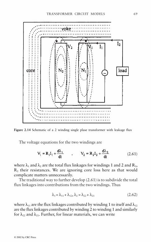
TRANSFORMER CIRCUIT MODELS 69
The voltage equations for the two windings are
(2.61)
where λ1 and λ2 are the total flux linkages for windings 1 and 2 and R1,R2 their resistances. We are ignoring core loss here as that wouldcomplicate matters unnecessarily.
The traditional way to further develop (2.61) is to subdivide the totalflux linkages into contributions from the two windings. Thus
λ1 = λ11 + λ12, λ2 = λ22 + λ21 (2.62)
where λ11 are the flux linkages contributed by winding 1 to itself and λ12
are the flux linkages contributed by winding 2 to winding 1 and similarlyfor λ22 and λ21. Further, for linear materials, we can write
Figure 2.14 Schematic of a 2 winding single plase transformer with leakage flux
© 2002 by CRC Press

TRANSFORMER CIRCUIT MODELS70
(2.63)
where L and M are self and mutual inductances and M12=M21=M. Thus(2.61) can be written
(2.64)
Assuming sinusoidal voltages and currents and reverting to phasornotation (bold faced type), (2.64) becomes
(2.65)
Separating the exciting current component out of I1 so that I1=Iex+I1 andusing amp-turn balance,
N1I'1=-N2I2 (2.66)
we obtain by substituting into (2.65).
(2.67)
Defining single winding leakage inductances as
(2.68)
the circuit model corresponding to (2.67) is given in Fig. 2.15. Thesesingle winding leakage inductance are for one winding with respect tothe other and thus depend on both windings.
© 2002 by CRC Press

TRANSFORMER CIRCUIT MODELS 71
We have introduced an ideal transformer in Fig. 2.15. In such adevice the currents into it are related by (2.66) and the voltages by
(2.69)
Using (2.66)-(2.69), we can write
(2.70)
or
Thus the circuit diagram in Fig. 2.15 can be redrawn as shown in Fig.2.16. The missing element in Fig. 2.15 or 2.16 is the core loss andpossibly capacitive effects. This could be added by putting a resistanceand capacitor in parallel with the voltage E1.
Figure 2.15 Circuit model of a 2 winding transformer under load
© 2002 by CRC Press

TRANSFORMER CIRCUIT MODELS72
It is instructive to develop a circuit model using a more fundamentalapproach which does not neglect the core non-linearities [MIT43]. Wewill utilize the concept of flux linkages per turn so that if λ is a fluxlinkage, N the number of turns linked, then Φ=λ/N is the flux linkage/turn. If the flux linked every turn of a circuit 100 %, then would be thetotal flux passing through the circuit.
Assume only coil 1 has current flowing through it. Let Φ11 be the fluxlinkage/turn in coil 1 produced by this current. Let Φ21 be the fluxlinkage/turn linking coil 2 produced by the current in coil 1. Define theleakage flux of coil 1 with respect to coil 2 as
(2.71)
Similarly, if only coil 2 is carrying current, we define the leakage fluxof coil 2 with respect to coil 1 as
(2.72)
where Φ22 is the flux linkage/turn linking coil 2 and Φ12 is the fluxlinkage/turn linking coil 1 produced by current in coil 2. Referring toFig. 2.14, we note that much of the flux produced by coil 1 or 2 flows inthe core and thus links both coils. Most of the remaining flux will havepaths in air or only partially in the core. Thus the leakage flux associated
Figure 2.16 Circuit model of a 2 winding transformer under load referred to theprimary side
© 2002 by CRC Press

TRANSFORMER CIRCUIT MODELS 73
with either coil consists of this remaining flux which has a large part ofits path in air or oil. Therefore, the mmf required to produce it will bealmost entirely in oil or air which means that it, as well as the current,will be linearly related to the leakage flux. In other words, non-linearitiesin the core will have little impact on the leakage flux. Thus the singlewinding leakage inductances defined as
(2.73)
will be essentially constant.From (2.62) we see that the total flux linking winding 1 and 2 can be
expressed as
(2.74)
Substituting from (2.71) and (2.72),
(2.75)
Letting Φ=Φ12+Φ21 and using (2.73), (2.75) becomes
(2.76)
so that the voltage equations (2.61) become
(2.77)
Φ is the sum of the fluxes linking one coil and produced by the other.In order to add these legitimately, we need to assume that the materialcharacteristics are linear. However, we can, at this stage, assume thatthese mutual fluxes are produced by the combined action of the currentsacting simultaneously. This will allow non-linear effects to be includedand Φ can therefore no longer be regarded as the sum of separate fluxes.
As before, we expect the core excitation current, Iex, to be supplied bythe primary coil so that
I1=Iex+I1 (2.78)
© 2002 by CRC Press
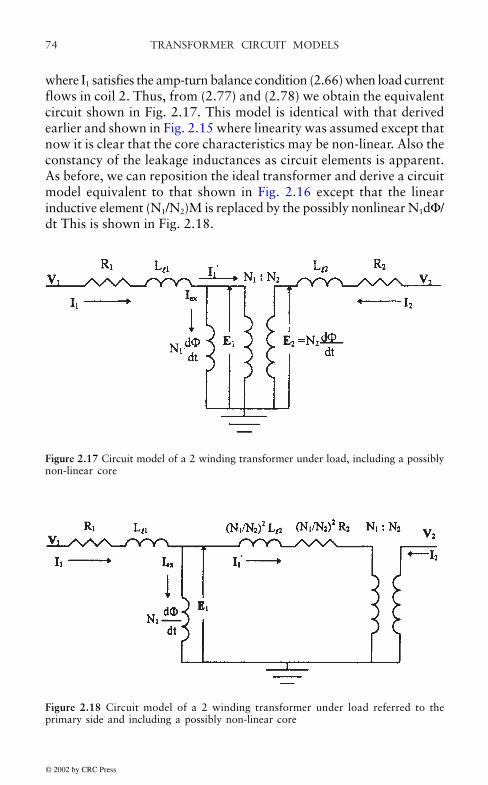
TRANSFORMER CIRCUIT MODELS74
where I1 satisfies the amp-turn balance condition (2.66) when load currentflows in coil 2. Thus, from (2.77) and (2.78) we obtain the equivalentcircuit shown in Fig. 2.17. This model is identical with that derivedearlier and shown in Fig. 2.15 where linearity was assumed except thatnow it is clear that the core characteristics may be non-linear. Also theconstancy of the leakage inductances as circuit elements is apparent.As before, we can reposition the ideal transformer and derive a circuitmodel equivalent to that shown in Fig. 2.16 except that the linearinductive element (N1/N2)M is replaced by the possibly nonlinear N1dΦ/dt This is shown in Fig. 2.18.
Figure 2.17 Circuit model of a 2 winding transformer under load, including a possiblynon-linear core
Figure 2.18 Circuit model of a 2 winding transformer under load referred to theprimary side and including a possibly non-linear core
© 2002 by CRC Press
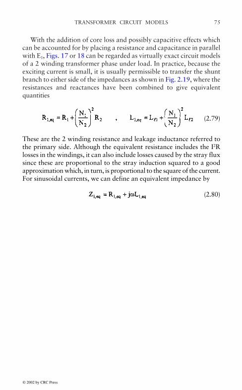
TRANSFORMER CIRCUIT MODELS 75
With the addition of core loss and possibly capacitive effects whichcan be accounted for by placing a resistance and capacitance in parallelwith E1, Figs. 17 or 18 can be regarded as virtually exact circuit modelsof a 2 winding transformer phase under load. In practice, because theexciting current is small, it is usually permissible to transfer the shuntbranch to either side of the impedances as shown in Fig. 2.19, where theresistances and reactances have been combined to give equivalentquantities
(2.79)
These are the 2 winding resistance and leakage inductance referred tothe primary side. Although the equivalent resistance includes the I2Rlosses in the windings, it can also include losses caused by the stray fluxsince these are proportional to the stray induction squared to a goodapproximation which, in turn, is proportional to the square of the current.For sinusoidal currents, we can define an equivalent impedance by
(2.80)
© 2002 by CRC Press
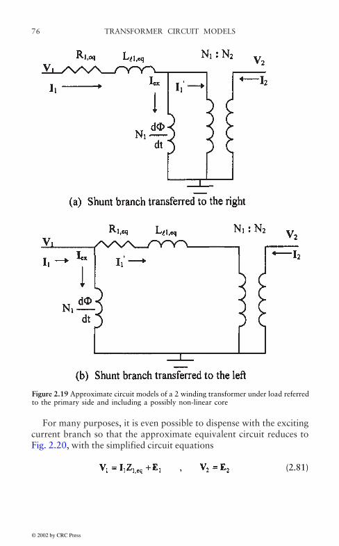
TRANSFORMER CIRCUIT MODELS76
For many purposes, it is even possible to dispense with the excitingcurrent branch so that the approximate equivalent circuit reduces toFig. 2.20, with the simplified circuit equations
(2.81)
Figure 2.19 Approximate circuit models of a 2 winding transformer under load referredto the primary side and including a possibly non-linear core
© 2002 by CRC Press

TRANSFORMER CIRCUIT MODELS 77
Using (2.66), with I1'=I1 since we are ignoring exciting current, and(2.69), we can write for (2.81)
]or (2.82)
Letting E1'=V1 and E2'=(N2/N1)V1, (2.82) becomes
(2.83)
where E1'/E2'=N1/N2. The circuit model for (2.83) is shown in Fig. 2.21where
(2.84)
Z2,eq is the equivalent impedance referred to the secondary side. It shouldnoted that the equivalent circuits with the core excitation branch included
Figure 2.20 Approximate circuit model of a 2 winding transformer under load referredto the primary side and ignoring core excitation
© 2002 by CRC Press
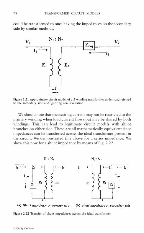
TRANSFORMER CIRCUIT MODELS78
could be transformed to ones having the impedances on the secondaryside by similar methods.
Figure 2.21 Approximate circuit model of a 2 winding transformer under load referredto the secondary side and ignoring core excitation
We should note that the exciting current may not be restricted to theprimary winding when load current flows but may be shared by bothwindings. This can lead to legitimate circuit models with shuntbranches on either side. These are all mathematically equivalent sinceimpedances can be transferred across the ideal transformer present inthe circuit. We demonstrated this above for a series impedance. Weshow this now for a shunt impedance by means of Fig. 2.22.
Figure 2.22 Transfer of shunt impedances across the ideal transformer
© 2002 by CRC Press

TRANSFORMER CIRCUIT MODELS 79
In Fig 22a, we have the relationships
(2.85)
Manipulating these equations, we obtain
(2.86)
From Fig. 2.22b, we have I2=I2'+I2,ex and I1/I2'=-N2/N1. Using these, (2.86)becomes
(2.87)
Thus the equivalent shunt impedance on the secondary side is obtainedin the same manner as for series impedances as is seen by comparing(2.84). The voltage and currents transform in the usual way across theideal transformer in both circuits of Fig. 2.22.
We see from Fig. 2.20 and 2.21 that if the shunt branch is ignored sothat the exciting current is zero and equal and opposite amp-turns flowin the 2 coils, then the inductance of this configuration is the 2 windingleakage inductance. This can then be obtained from the energy in themagnetic field by methods to be described later.
We mentioned earlier that in modern power transformers, whichtypically have very low core exciting current, capacitive effects can beimportant in situations where the core characteristics play a role. Weindicated that one way of including these effects was by placing a shuntcapacitance across the core. However, for greater accuracy, a bettermethod is to use the circuit model shown in Fig. 2.23 or one of itsequivalents. This model also includes the core losses by means of a coreresistance. There are shunt capacitances across the input and output sothat even if one of the coils is open circuited, the shunt capacitancewould act as a load so that current would flow in both windings. Thismodel has been found to accurately reproduce test results over afrequency range near the power frequency.
© 2002 by CRC Press

TRANSFORMER CIRCUIT MODELS80
When the core has non-linear Φ vs Iex characteristics, since E1= N1
dΦ/dt, a sinusoidal E1 will result in a non-sinusoidal Iex, For Φreasonably below saturation, the non-linearities are mild enough thatIex can be considered sinusoidal for most purposes when the primarycircuit is driven by a sinusoidal voltage. In this case N1 dΦ/dt can bereplaced by a magnetizing inductance or reactance. As the transformeris driven into saturation, the exciting current becomes nonsinusoidaland also constitutes a greater fraction of the load current. In this case, itbegins to matter which coil carries it. As was seen in the extreme case ofinrush current, the exciting current depended on the mean area of thecoil through which it flowed. In this extreme, the circuit modals wehave developed here are no longer applicable. One would need to workdirectly with flux linkages. One could define non-linear inductancesand mutual inductances as in (2.63) but it would no longer be true thatM12= M21. Also the L’s and M’s would depend on possibly both I1 and I2.
2.7 PER UNIT SYSTEM
Transformer impedances, along with other quantities such as voltagesand currents are often expressed in the per unit (p.u.) system. In thissystem, these quantities are expressed as a ratio with respect to thetransformer’s nominal or rated phase quantities. Thus, if the rated or basephase voltages are Vb1, Vb2 and the base currents are Ib1, Ib2 where 1 and 2refer to the primary and secondary sides, then the base impedances are
Figure 2.23 Circuit model of a 2 winding transformer under load, including a possiblynon-inear core, core losses, and capacitative effects
© 2002 by CRC Press

TRANSFORMER CIRCUIT MODELS 81
(2.88)
The rated or base voltages, currents, and impedances are assumed totransfer from one side to the other by means of the ideal transformerrelationships among voltages, currents, and impedances. These basequantities are all taken to be positive. Thus the minus sign is neglectedin the base current transfer across sides. Hence, it can be shown that thebase power, Pb, is the same on both sides of a transformer,
Pb=Vb1 Ib1=Vb2 Ib2 (2.89)
In an actual transformer, the real power into a transformer is nearly thesame as that leaving it on the secondary side. This is because thetransformer losses are a small fraction of the power transferred,
The primary side voltage, V1, current, I1, and equivalent impedance,Z1,eq, are expressed in the per unit system by
(2.90)
and similarly for the secondary quantities. Often the p.u, values aremultiplied by 100 and expressed as a percentage. However, it is best notto use the percentage values in calculations since this can lead to errors.As indicated in (2.90), we use lower case letters to denote p.u. quantities.
Since the base quantities transfer across the ideal transformer in thesame manner as their corresponding circuit quantities, the p.u. valuesof the circuit quantities are the same on both the primary and secondarysides. Thus the 1 or 2 subscripts can be dropped when referring to p.u.quantities. Although voltages, currents, and impedances fortransformers of greatly different power ratings can differ considerably,their per unit values tend to be very similar. This can facilitatecalculations since one has a pretty good idea of the magnitudes of thequantities being calculated. Thus, the 2 winding leakage impedanceswhen expressed in the p.u system are generally in the range of 5–15 %for all power transformers. The exciting currents of modern powertransformers are typically ~0.1% in the p.u. system. This is also theirpercentage of the rated load current since this has the value of 1 or 100% in the p.u, system. The 2 winding resistances which account for thetransformers losses can be obtained in the p.u. system by noting that
© 2002 by CRC Press

TRANSFORMER CIRCUIT MODELS82
modern power transformers are typically >99.5 % efficient. This meansthat <0.5 % of the rated input power goes into losses. Thus we have
(2.91)
We omitted a 1 subscript on the per unit equivalent resistance, r, since itis the same on both sides of the transformer. Using this and the aboveestimate of the leakage impedance in the p.u. system, x, for powertransformers, we can estimate the x/r ratio,
(2.92)
Thus 10 is probably a lower limit and, as previously shown, is highenough to allow discriminating inrush from fault current on the basis ofsecond harmonic analysis.
2.8 VOLTAGE REGULATION
At this point, it is useful to discuss the topic of voltage regulation as anapplication of the transformer circuit model just developed. In this context,the core characteristics do not play a significant role so we will use thesimplified circuit model of Fig. 2.21. Voltage regulation is defined asthe change in the magnitude of the secondary voltage between its opencircuited value and its value when loaded divided by the value whenloaded with the primary voltage held constant. We can represent theload by an equivalent impedance, ZL, and the relevant circuit is shownin Fig. 2.24. In the figure, we have shown a load current, IL, whereIL=-I2.
© 2002 by CRC Press

TRANSFORMER CIRCUIT MODELS 83
It is convenient to perform this calculation in the per unit system, Wewill use lower case letters to represent per unit quantities. Thus sincebase quantities transfer across the ideal transformer like theircorresponding physical quantities, we have
(2.93)
Therefore the ideal transformer can be eliminated from the circuit in theper unit system. Also, since z2,eq=z1,eq, we can drop the numerical subscriptand denote the equivalent transformer p.u, impedance by
z=r+jx (2.94)
where r is the p.u. equivalent resistance and x the p.u. 2 winding leakagereactance. Similarly we write
(2.95)
The p.u. circuit is shown in Fig. 2.25.
Figure 2.24 Approximate circuit models of a 2 winding transformer with load includedand referred to the secondary side
© 2002 by CRC Press

TRANSFORMER CIRCUIT MODELS84
Thus when the secondary terminal is open circuited so zL and itsground connection are missing in Fig. 2.25, we obtain for the opencircuited value of v2,
v2,oc=v1 (2.96)
We assume that ν1 is a reference phasor (zero phase angle) and v1 istherefore its magnitude. When the load is present, we have
(2.97)
Thus, from (2.97),
(2.98)
Hence the voltage regulation is given by
(2.99)
It is customary to express zL in terms of the load voltage and currentvia (2.97),
Figure 2.25 The circuit of Fig. 2.24 shown in the p.u. system
© 2002 by CRC Press

TRANSFORMER CIRCUIT MODELS 85
(2.100)
where θ=θν”θi is the angle by which the voltage leads the current. For aninductive load, θ is positive. Letting v2 and iL represent the magnitudesof the load voltage and current, i.e. dropping the magnitude signs, theimpedance ratio in (2.99) can be written
(2.101)
Substituting (2.101) into (2.99), we get
(2.102)
Since z is generally small compared with zL, the terms other than unityin (2.102) are small compared to unity. Using the approximation forsmall ε,
(2.103)
the regulation is given to second order in z/zL by
(2.104)
© 2002 by CRC Press

87
3. REACTANCE CALCULATIONS
Summary Leakage reactances are calculated for transformers havingup to six separate windings per leg but with 2 or 3 terminals per phase.These calculations may be applied to single phase units or to one phaseof a 3 phase unit. Windings may be connected in series or auto-connected.In addition, tap windings or series taps within a winding may beidentified. Terminal-terminal and positive/negative sequence leakagereactances are calculated, as well as the T-equivalent circuit modelleakage reactances for 3 terminal transformers. Expressions for per-unitquantities are also given. When taps are present within a winding or asseparate windings, calculations are performed for the all in, all out, andcenter or neutral position and for all combinations if more than onetype of tap is present. The calculations are based on a 2 winding reactanceformula which assumes that the windings are uniform along their length,with a correction for end fringing flux. This has been found to be veryaccurate for most purposes but, if greater accuracy is desired, a bettertwo winding reactance calculation could be substituted without changingmost of the formulas presented here.
3.1 INTRODUCTION
The reactance calculations performed here are on a per phase basis sothey would apply to a single phase unit or to one phase of a three phasetransformer. The phase can have up to six windings, interconnected insuch a way that only 2 or 3 terminals (external or buried) result. Thusauto-transformers, with or without tertiary, are included as well astransformers with tap windings. it should be noted that these reactancesare positive or negative sequence reactances. Zero sequence reactancesare somewhat sensitive to the three phase connection and to whether thetransformer is core-form or shell-form, but this does not appear to betrue for the positive/negative sequence reactances. Thus, in the followingdiscussion, we will be dealing with a single phase system which may ormay not be part of a 3 phase system.
It is usually desirable to design some reactance into a transformer inorder to limit any fault current. In addition, these reactances determine
© 2002 by CRC Press

REACTANCE CALCULATIONS88
the voltage regulation of the unit. Hence it is desirable at the designstage to be able to calculate these reactances based on the geometry ofthe coils and core and the nature of the (single phase) windinginterconnections.
We begin by discussing ideal transformers, i.e. having no reactanceor resistance, since real transformers are usually described by addinglumped resistance and reactance circuit elements to a model of an idealtransformer. The following references have been used in this chapter:[MIT43], [Lyo37], [Blu51], [Wes64].
3.2 IDEAL TRANSFORMERS
In an ideal 2 winding transformer as depicted in Fig. 3.1, the entire fluxφ links both windings so that, by Faraday’s law, the induced emf’s aregiven by
(3.1)
Hence
(3.2)
We use the convention that the current is positive when entering thepositive terminal and that the fluxes generated by these positive currentsadd.
Figure 3.1 Ideal 2 winding transformer
© 2002 by CRC Press

89REACTANCE CALCULATIONS
In an ideal transformer, zero mmf is required to generate the flux sothat
N1I1+N2I2=0 (3.3)
which implies
(3.4)
i.e., the secondary current I2 is leaving terminal 2 (negative) when theprimaiy current I1 enters terminal 1. Also, from the above equations
(3.5)
i.e. the instantaneous power entering terminal 1 equals the power leavingterminal 2 so that the unit is lossless as expected.
For a 3 winding unit, the above formulas become
(3.6)
and
N1I1+N2I2+N3I3=0 (3.7)
which imply
E1I1+E2I2+E3I3=0 (3.8)
i.e. the net power into the unit is 0, or the power entering equals thepower leaving. The generalization to more than 3 windings isstraightforward.
If the ideal transformer has a load of impedance Z2 connected to itssecondary terminals as shown in Fig. 3.2, we have the additionalequation
E2=-I2Z2 (3.9)
where -I2 is the load current, usually denoted IL.
© 2002 by CRC Press

REACTANCE CALCULATIONS90
But from the above equations,
(3.10)
Thus, as seen from the primary terminals, the load appears as animpedance Z1,
E1=I1Z1 (3.11)
where
(3.12)
At this point we introduce per-unit values. That is, we choose basevalues for voltages, currents, etc. and express the actual voltages, currents,etc. as ratios with respect to these base values. Only two independentbase values need to be chosen and these are usually taken as power orVI and voltage V. The base power is normally taken as the VI rating ofthe unit per phase and the voltage taken as the open circuit rated phasevoltage of each terminal. Thus we have a (VI)b and V1b, V2b, … where bdenotes base value. From these we derive base currents of
(3.13)
and base impedances
Figure 3.2 Ideal 2 winding transformer with a load on its secondary terminals
© 2002 by CRC Press

91REACTANCE CALCULATIONS
(3.14)
Letting small letters denote per-unit quantities, we have
(3.15)
Ignoring core excitation, at no load we have V1=E1, etc. so that from(3.6), (3.13), (3.14),
(3.16)
since everything is on a common VI base.In terms of per-unit quantities, we have for an ideal transformer
(3.17)
and, from (3.7) and (3.16)
Therefore
i1+i2+i3=0 (3.18)
Thus an ideal 3-circuit transformer can be represented by a one circuitdescription as shown in Fig. 3.3, if per-unit values are used. This alsoholds if more than 3 circuits are present.
, etc.
etc.
, etc.
, etc.
© 2002 by CRC Press
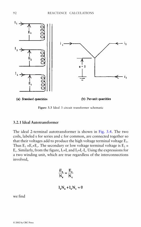
REACTANCE CALCULATIONS92
3.2.1 Ideal Autotransformer
The ideal 2-terminal autotransformer is shown in Fig. 3.4. The twocoils, labeled s for series and c for common, are connected together sothat their voltages add to produce the high voltage terminal voltage E1.Thus E1 =Es+Ec. The secondary or low voltage terminal voltage is E2 =Ec. Similarly, from the figure, I1=Is and I2=Ic-Is. Using the expressions fora two winding unit, which are true regardless of the interconnectionsinvolved,
Figure 3.3 Ideal 3 circuit transformer schematic
we find
© 2002 by CRC Press

93REACTANCE CALCULATIONS
Thus
(3.19)
so that the effective turns ratio as seen by the terminals is n=(Nc+Ns)/Nc. Any impedances on the low voltage terminal could be transferredto the high voltage circuit by the square of this turns ratio.
The co-ratio is defined as
(3.20)
Figure 3.4 Ideal autotransfonner
© 2002 by CRC Press
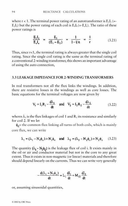
REACTANCE CALCULATIONS94
where r < 1. The terminal power rating of an autotransformer is E1I1 (=-E2I2) but the power rating of each coil is ESIS (=-EcIc). The ratio of thesepower ratings is
(3.21)
Thus, since r<1, the terminal rating is always greater that the single coilrating. Since the single coil rating is the same as the terminal rating ofa conventional 2-winding transformer, this shows an important advantageof using the auto connection,
3.3 LEAKAGE IMPEDANCE FOR 2-WINDING TRANSFORMERS
In real transformers not all the flux links the windings. In addition,there are resistive losses in the windings as well as core losses. Thebasic equations for the terminal voltages are now given by
(3.22)
wheres λ1 is the flux linkages of coil 1 and R1 its resistance and similarlyfor coil 2. If we let
= the common flux linking all turns of both coils, which is mainly
core flux, we can write
(3.23)
The quantity is the leakage flux of coil i. It exists mainly inthe oil or air and conductor material but not in the core to any greatextent. Thus it exists in non-magnetic (or linear) materials and thereforeshould depend linearly on the currents. Thus we can write very generally
or, assuming sinusoidal quantities,
© 2002 by CRC Press
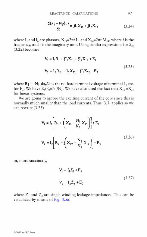
95REACTANCE CALCULATIONS
(3.24)
where I1 and I2 are phasors, X11=2πf L1 and X12=2πf M12, where f is thefrequency, and j is the imaginary unit. Using similar expressions for λ2,(3.22) becomes
(3.25)
where is the no-load terminal voltage of terminal 1, etc.for E2. We have E1/E2=N1/N2. We have also used the fact that X12 =X21
for linear systems.We are going to ignore the exciting current of the core since this is
normally much smaller than the load currents. Thus (3.3) applies so wecan rewrite (3.25)
(3.26)
or, more succinctly,
(3.27)
where Z1 and Z2 are single winding leakage impedances. This can bevisualized by means of Fig. 3.5a.
© 2002 by CRC Press
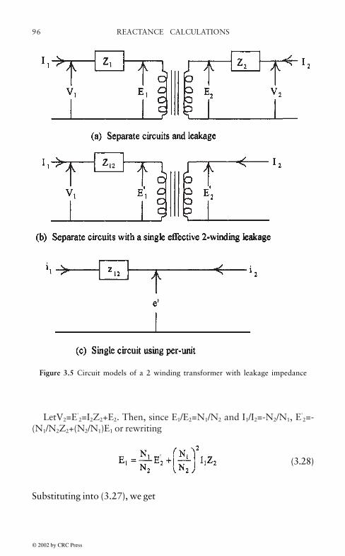
REACTANCE CALCULATIONS96
LetV2=E'2=I2Z2+E2. Then, since E1/E2=N1/N2 and I1/I2=-N2/N1, E'
2=-(N1/N2Z2+(N2/N1)E1 or rewriting
(3.28)
Substituting into (3.27), we get
Figure 3.5 Circuit models of a 2 winding transformer with leakage impedance
© 2002 by CRC Press

97REACTANCE CALCULATIONS
(3.29)
We see that (3.29) can be expressed in terms of a single effectiveimpedance Z12=Z1+(N1/N2)2 Z2,
(3.30)
where E21/E22=N1/N2. The circuit model for this is shown in Fig. 3.5b.Using per-unit values, the picture in Fig. 3.5c applies. Note that E1/E2
=E'1/E’2=N1/N2 but that E1≠E'1, E2≠E'2 except at no load.Thus a two winding transformer is characterized by a single value of
leakage impedance Z12 which has both resistive and reactivecomponents,
Z12 = R12 + jX12
where
(3.31)
and
referred to the primary winding. We can obtain expressions for referringquantities to the secondary winding by interchanging 1 and 2 in theabove formulas. In large power transformers X12>>R12 so we are normallyconcerned with obtaining leakage reactances.
In terms of previously defined quantities,
© 2002 by CRC Press
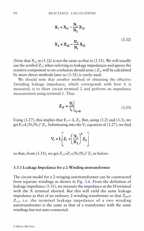
REACTANCE CALCULATIONS98
(3.32)
(Note that X12 in (3.32) is not the same as that in (3.31). We will usuallyuse the symbol Z12 when referring to leakage impedances and ignore theresistive component so no confusion should arise.) Z12 will be calculatedby more direct methods later so (3.32) is rarely used.
We should note that another method of obtaining the effective2winding leakage impedance, which corresponds with how it ismeasured, is to short circuit terminal 2 and perform an impedancemeasurement using terminal 1. Thus
(3.33)
Using (3.27), this implies that E2 = -I2 Z2. But, using (3.2) and (3.3), weget E1=I1(N1/N2)2 Z2. Substituting into the V1 equation of (3.27), we find
so that, from (3.33), we get Z12=Z1+(N1/N2)2 Z2 as before.
3.3.1 Leakage Impedance for a 2-Winding utotransformer
The circuit model for a 2-winging autotransformer can be constructedfrom separate windings as shown in Fig. 3.6. From the definition ofleakage impedance (3.33), we measure the impedance at the H terminalwith the X terminal shorted. But this will yield the same leakageimpedance as that of an ordinary 2-winding transformer so that ZHX=Z12, i.e. the terminal leakage impedance of a two windingautotransformer is the same as that of a transformer with the samewindings but not auto-connected.
© 2002 by CRC Press

99REACTANCE CALCULATIONS
3.4 LEAKAGE IMPEDANCES FOR 3-WINDING TRANSFORMERS
We can go through the same arguments for a 3-winding transformer,isolating the flux common to all coils φc, and expressing the leakageflux for each coil, which exists in non-magnetic materials, in terms ofself and mutual inductances which are constants. We obtain
(3.34)
The order of the suffixes is irrelevant, since for linear materials (constantpermeability) Xij=Xji.
Using the same assumptions as before concerning the neglect of coreexcitation, equation (3.7), we substitute I3=-(N1/N3) I1-(N2/N3) I2 in the
Figure 3.6 Circuit model of a 2 winding autotransformer with leakage impedance,based on a seperate windings circuit model
© 2002 by CRC Press

REACTANCE CALCULATIONS100
first 2 equations and I2 =-(N1/N2) I1-(N3/N2) I3 in the third equation of(3.34) to obtain
(3.35)
Now add and subtract from the first equation,
add and subtract from the second, and add and
subtract from the third equation of (3.35) to obtain
(3.36)
© 2002 by CRC Press

101REACTANCE CALCULATIONS
Substituting for I3=-(N1/N3) I1-(N2/N3) I2 in the term in brackets in thelast equation, we obtain
(3.37)
Comparing the terms in brackets of the resulting V1, V2, V3 equations,we find, using (3.6),
(3.38)
Therefore, labeling the terms in brackets E'1, E'2, E'3, we obtain
(3.39)
where
and
(3.41)
Here Z1, Z2, Z3 are the single winding leakage impedances and theapplicable multi-circuit model is shown in Fig. 3.7a. If we expressquantities in terms of per unit values, the single circuit description ofFig. 3.7b applies. This is possible because (3.41) implies e'1=e'2=e'3=e'and by equation (3.18). This figure should be compared with Fig. 3.3.
(3.40)
© 2002 by CRC Press

REACTANCE CALCULATIONS102
Since the single winding leakage impedances are not directly measuredor easily calculated, it is desirable to express these in terms of 2-windingleakage impedances. We will refer to these 2-winding leakageimpedances as Z12, Z13, Z23 which correspond to the notation Z12 usedpreviously for the two winding case. Thus to measure the 2-windingleakage impedance between winding 1 and 2, we short circuit 2, opencircuit 3, and measure the impedance at terminal 1,
(3.42)
From (3.39) we see that this implies I2 Z2+E'2=0. Using (3.6) and (3.7),we find for Z12 and similarly for Z13 and Z23
Figure 3.7 Circuit models of a 3 winding transformer with leakage impedance
(3.43)
© 2002 by CRC Press

103REACTANCE CALCULATIONS
The subscript ordering is chosen so that the second subscript refers tothe shorted winding. The expression changes if we reverse subscripts,according to
(3.44)
Solving (3.43) for the Zi’s, we get
Using per-unit values, where Z1b is the base impedance of circuit 1 sothat z12=Z12/Z1b, etc. and Z1=z1/Z1b, etc. we find, using (3.16), that (3.45)can be expressed as
z1=(z12+z13-z23)/2
z2=(z12+z23-z13)/2 (3.46)
z3=(z13+z23-z12)/2
Similarly (3.43) becomes, in per-unit terms,
(3.47)
(3.45)
© 2002 by CRC Press

REACTANCE CALCULATIONS104
The term was added and subtracted from the V3 equationabove.
3.4.1 Leakage Impedances for an Autotransfonner with Tertiary
The autotransformer with tertiary circuit model can be obtained byinterconnecting elements of the 3-winding transformer circuit model asshown in Fig. 3.8. Here the notation corresponds to that of Fig. 3.7a.The problem is to re-express this in terms of terminal quantities. Thusthe appropriate terminal 1 voltage is V1+V2 and the appropriate terminal2 current is I2-I1. Using (3.39),
(3.48)
Substituting from (3.7) into this equation and the V2 and V3 equationsof (3.39), we obtain after some algebraic manipulations,
(3.49)
© 2002 by CRC Press

105REACTANCE CALCULATIONS
We see that the terms in brackets satisfy
(3.50)
Labeling these terms in brackets EH, EX, EY, we can rewrite (3.49)
(3.51)
where VH=V1+V2, VX=V2, VY=V3, IH=I1, IX=I2-I1, IY=I3, and
Figure 3.8 3 winding autotransformer circuit model, derived from the 3 separatewinding circuit model
(3.52)
© 2002 by CRC Press

REACTANCE CALCULATIONS106
In terms of the measured two terminal impedances, we have as before
(3.53)
Rewriting (3.7), we find
N1I1+N2(I2–I1)+N2I1+N3I3
= (N1+N2)IH+N2IH+N2IX=0 (3.54)
From (3.53) with (3.50), (3.51) and (3.54), we obtain
Thus the circuit model shown in Fig. 3.9a looks like that of Fig. 3.7awith H, X, Y substituted for 1, 2, 3.
Figure 3.9 Circuit models of a 3 winding autotransformer based on terminal parameters
© 2002 by CRC Press

107REACTANCE CALCULATIONS
(3.55)
At this point, it is worthwhile to revert to per-unit quantities. Becauseof the auto connection, we have, again choosing the VI per phase ratingof the unit and the rated (no-load) terminal voltages per phase, (VI)b,VHb, VXb, VYb,
since (VI)b is the same for each terminal. From (3.54), we have on a perunit basis,
iH+iX+iY=0 (3.57)
Similarly from (3.50), on a per-unit basis
eH=eX=eY=e (3.58)
On a per-unit basis, (3.55) becomes, using (3.56)
(3.59)
where the same VI base is used for all the terminals. Solving these forzH, zX, zY, we obtain a set of equations similar to (3.46)
(3.56)
© 2002 by CRC Press
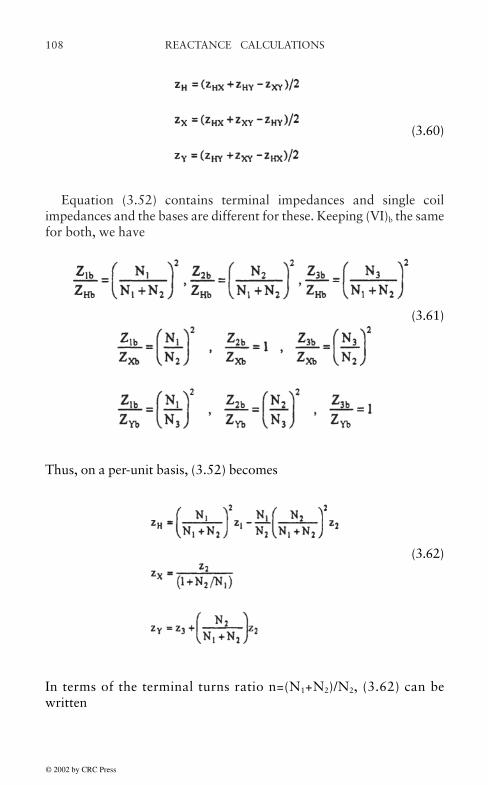
REACTANCE CALCULATIONS108
(3.60)
Equation (3.52) contains terminal impedances and single coilimpedances and the bases are different for these. Keeping (VI)b the samefor both, we have
Thus, on a per-unit basis, (3.52) becomes
(3.61)
In terms of the terminal turns ratio n=(N1+N2)/N2, (3.62) can bewritten
(3.62)
© 2002 by CRC Press
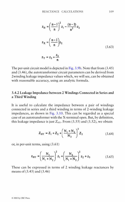
109REACTANCE CALCULATIONS
(3.63)
The per-unit circuit model is depicted in Fig. 3.9b. Note that from (3.45)and (3.46), the autotransformer circuit parameters can be derived from2winding leakage impedance values which, we will see, can be obtainedwith reasonable accuracy, using an analytic formula.
3.4.2 Leakage Impedance between 2 Windings Connected in Series anda Third Winding
It is useful to calculate the impedance between a pair of windingsconnected in series and a third winding in terms of 2-winding leakageimpedances, as shown in Fig. 3.10. This can be regarded as a specialcase of an autotransformer with the X-terminal open. But, by definition,this leakage impedance is just ZHY. From (3.55) and (3.52), we obtain
(3.64)
or, in per-unit terms, using (3.61)
(3.65)
These can be expressed in terms of 2 winding leakage reactances bymeans of (3.45) and (3.46)
© 2002 by CRC Press
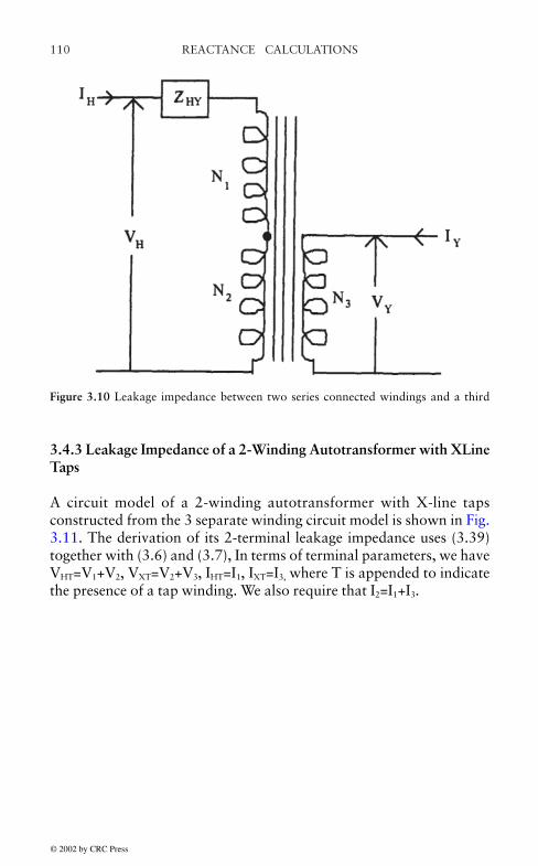
REACTANCE CALCULATIONS110
3.4.3 Leakage Impedance of a 2-Winding Autotransformer with XLineTaps
A circuit model of a 2-winding autotransformer with X-line tapsconstructed from the 3 separate winding circuit model is shown in Fig.3.11. The derivation of its 2-terminal leakage impedance uses (3.39)together with (3.6) and (3.7), In terms of terminal parameters, we haveVHT=V1+V2, VXT=V2+V3, IHT=I1, IXT=I3, where T is appended to indicatethe presence of a tap winding. We also require that I2=I1+I3.
Figure 3.10 Leakage impedance between two series connected windings and a third
© 2002 by CRC Press

111REACTANCE CALCULATIONS
Thus
Figure 3.11 Circuit model of a 2 winding autotransformer with X-line taps, derivedfrom the 3 separate winding circuit
Substitute I3=-(N1/N3)I1-(N2/N3)I2 into the VHT equation and I1=-(N2 /N1)I2-(N3/N1)I3 into the VXT equation to obtain
(3.66)
(3.67)
© 2002 by CRC Press

REACTANCE CALCULATIONS112
Add and subtract from the VHT equation and add and
subtract from the VXT equation to obtain, after some
algebraic manipulations,
(3.68)
which can be rewritten
VHT=IHTZHT+EHT . VXT=IXTZXT+EXT (3.69)
where
(3.70)
To obtain the 2 terminal leakage impedance, we use the definition
(3.71)
We have
(3.72)
and from (3.7) we obtain
N1I1+N2(I1+I3)+N3I3=(N1+N2)I1+(N2+N3)I3
=(N1+N2)IHT+(N2+N3)IXT=0 (3.73)
Using (3.69) together with (3.72) and (3.73), we obtain from (3.71)
© 2002 by CRC Press

113REACTANCE CALCULATIONS
(3.74)
Using (3.70), this becomes
(3.75)
On a per-unit basis, using a fixed (VI)b and, noting that
we find
(3.76)
This is the two terminal leakage impedance of a 2 windingautotransformer with X-line taps. It can be expressed in terms of the 2winding leakage impedances via equations (3.45) and (3.46).
3.4.4 More General Leakage Impedance Calculations
The cases considered so far cover most of the configurations encounteredin practice. However, other situations can be covered by using theseresults as building blocks. For example, to obtain the leakage impedancebetween three windings connected in series and a fourth winding, useformula (3.64) or (3.65) to obtain the leakage impedance between thefourth winding and two of the other windings connected in series. Thenadd the third winding. Considering the two series winding as a singlewinding, calculate the single winding impedances for this new “threewinding” system and reapply (3.64) or (3.65).
Another example would be an autotransformer with tertiary andXline taps. The circuit model for this can be derived from the 2-winding
© 2002 by CRC Press

REACTANCE CALCULATIONS114
autotransformer with X-line taps by adding a tertiary winding. Thenthe 2-terminal leakage reactance, equation (3.75) or (3.76), between theseries+common and X-line tap+common, together with the 2-terminalleakage reactances between the tertiary and the series+common andbetween the tertiary and the X-line tap+common can be used toconstruct a 3-terminal impedance model similar to Fig. 3.9.
3.5 TWO WINDING LEAKAGE REACTANCE FORMULA
All of the reactance circuit parameters obtained here for 2 or 3 terminaltransformers can be expressed in terms of 2-winding leakage reactances.These can be calculated by advanced analytical techniques or finiteelement methods which solve Maxwell’s equations directly. Thesemethods are especially useful if the distribution of amp-turns along thewinding is non-uniform, due, for example, to tapped out sections orthinning in sections of windings adjacent to taps in neighboring windings.However, simpler idealized calculations have proven adequate in practice,particularly at the early design stage. These simpler calculations willbe discussed here but, however these 2-winding reactances are obtained,they can be used directly in the formulas derived previously.
The simple reactance calculation assumes that the amp-turns areuniformly distributed along the windings. It also treats the windings asif they were infinitely long insofar as the magnetic field is concerned,although a correction for fringing at the ends is included in the finalformula. The parameters of interest are shown in Fig. 3.12. If thewindings were infinitely long and the amp-turns per unit length wereequal for the two windings then the magnetic field as a function ofradius would be proportional to the amp-turn distribution shown in Fig.3.12b, i.e. in the SI system,
H(r)=NI(r)/h (3.77)
where NI(r) is the function of r shown in the figure, linearly increasingfrom 0 through winding 1, remaining constant in the gap, and decreasingto 0 through winding 2. H is independent of the z-coordinate in thismodel and points vectorially in the z-direction. The flux density istherefore
B(r)=µoH(r)=µoNI(r)/h (3.78)
© 2002 by CRC Press
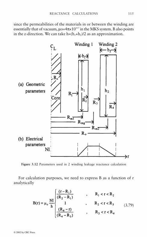
115REACTANCE CALCULATIONS
For calculation purposes, we need to express B as a function of ranalytically
since the permeabilities of the materials in or between the winding areessentially that of vacuum, µo=4π×10"7 in the MKS system. B also pointsin the z-direction. We can take h=(h1+h2)/2 as an approximation.
Figure 3.12 Parameters used in 2 winding leakage reactance calculation
(3.79)
© 2002 by CRC Press
REACTANCE CALCULATIONS116
In terms of mean radii Rm, thicknesses b, and gap g shown in Fig. 3.12,(3.81) can be written
(3.82)
Because the terms in b12 and b2
2 are so much smaller that the others, wedrop them and find, using (3.80)
(3.83)
The leakage reactance is XL=2πfL so we get
(3.84)
On a per-unit basis,
where the Ri are indicated in Fig. 3.12. The leakage inductance, L, canbe obtained from the magnetic energy in the leakage field by means ofthe expression
(3.80)
Substituting (3.79) into the integral, we get
(3.81)
© 2002 by CRC Press

117REACTANCE CALCULATIONS
where (VI)b is the base volt-amps per phase and Vb/N is the base Volts/turn. Letting x denote the per-unit reactance, where x=XL/Xb, we get
(3.85)
in MKS units at 60 Hz or
(3.86)
when lengths are measured in inches. This same result could have beenobtained by consideration of flux-linkages but the effort required wouldhave been greater.
In order to correct for fringing, it has been found that a goodapproximation is to increase h by the amount
s=0.32(Ro-Rc) (3.87)
where Ro is the outer radius of the outermost coil and Rc is the coreradius. Thus we obtain
(3.88)
© 2002 by CRC Press

4. FAULT CURRENT CALCULATIONS
Summary Fault currents at the terminals and in the windings arecalculated for transformers subjected to the standard faults: 3-phase lineto ground, single phase line to ground, line to line, and double line toground. Since these faults result in unbalanced currents in the 3 phasesystem, except for 3-phase faults, the method of symmetrical componentsis introduced and used in the fault analysis. In this method, the unbalancedvoltages and currents are replaced by balanced systems of positive,negative, and zero sequence quantities. The circuits associated witheach of these sequences can differ. After solving the sequence circuitequations, the unbalanced quantities are obtained by a reversetransformation. A 2-terminal per phase transformer is modeled using asingle leakage impedance and a 3-terminal per phase unit is modeledwith 3 leakage impedances (T-equivalent circuit). The leakageimpedances are the same for the positive and negative sequence circuitsbut can differ for the zero sequence circuit. The systems attached to theexternal terminals of the transformer are treated simply as a voltagesource in series with an impedance. An asymmetry factor is included toaccount for an initial transient surge which usually accompanies a fault.
4.1 INTRODUCTION
It is necessary to design transformers to withstand various possible faults,such as a short to ground of one or more phases. The high currentsaccompanying these faults, approximately 10 to 30 times normal, producehigh forces and stresses in the windings and support structure. Also,depending on the fault duration, significant amounts of heat may begenerated inside the unit. The design must accommodate the worst casefault which can occur from both the mechanical and thermal standpoints.
The first step in designing to withstand faults is to determine the faultcurrents in all the windings, which is the subject of this report. Since thisis an electrical problem, it requires a circuit model which includesleakage impedances of the transformer and also relevant systemimpedances. The system is typically represented by a voltage source in
© 2002 by CRC Press

FAULT CURRENT CALCULATIONS120
series with an impedance, since we are not interested here in detailedfault currents within the system external to the transformer. Thetransformer circuit model considered here is that of a 2 or 3 terminalper phase unit with all pairs of terminal leakage reactances given eitherfrom calculations or measurement (from these the T-equivalentreactances can be obtained). We ignore core excitation since, formodern power transformers, its effects on the fault currents arenegligible.
The transformers dealt with here are 3-phase units and the fault typesconsidered are: 3-phase line to ground, single phase line to ground, lineto line, and double line to ground. These are the standard fault typesand are important because they are most likely to occur on actualsystems. The transformer must be designed to withstand the worst ofthese fault types, or rather each coil must be designed to withstand theworst (highest current) fault it can experience. Note that each fault typerefers to a fault on any of the single phase terminals. For example, a 3-phase fault can occur on all the high voltage terminals (H1, H2, H3), allthe low voltage terminals (X1, X2, X3), or all the tertiary voltageterminals (Y1, Y2, Y3). Etc. for the other fault types. Note also that faultson a single phase system can be considered as 3-phase faults on a 3-phase system so that these are included automatically in the analysis offaults on 3-phase systems.
Since the fault types considered include faults which produceunbalanced conditions in a 3-phase system, probably the most efficientway of treating them is by the method of symmetrical components. Inthis method, an unbalanced set of voltages or currents can berepresented mathematically by sets of balanced voltages or currents,called sequence voltages or currents. These latter can then be analyzedby means of sequence circuit models. The final results are then obtainedby transforming the voltages and currents from the sequence analysisinto the voltages and currents of the real system. We will discuss thismethod in greater detail before proceeding with the specific faultanalyses.
It should also be noted that the circuit model calculations to bediscussed are for steady-state conditions, whereas actual faults wouldhave a transient phase where the currents can exceed their steady-statevalues for short periods of time. These enhancement effects are includedby means of an asymmetry factor. This factor takes into account theresistance and reactance present at the faulted terminal and isconsidered to be conservative from a design point of view. Thefollowing references have been used: [Ste62a], [Lyo37], [Blu51].
© 2002 by CRC Press
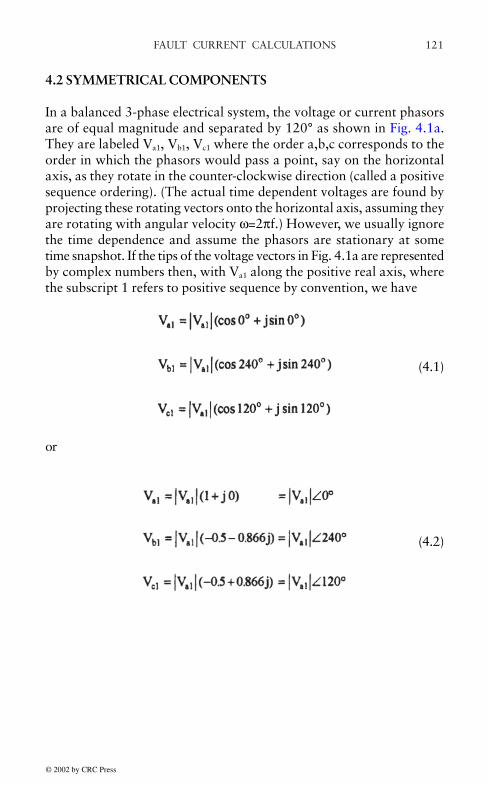
121FAULT CURRENT CALCULATIONS
4.2 SYMMETRICAL COMPONENTS
In a balanced 3-phase electrical system, the voltage or current phasorsare of equal magnitude and separated by 120° as shown in Fig. 4.1a.They are labeled Va1, Vb1, Vc1 where the order a,b,c corresponds to theorder in which the phasors would pass a point, say on the horizontalaxis, as they rotate in the counter-clockwise direction (called a positivesequence ordering). (The actual time dependent voltages are found byprojecting these rotating vectors onto the horizontal axis, assuming theyare rotating with angular velocity ω=2πf.) However, we usually ignorethe time dependence and assume the phasors are stationary at sometime snapshot. If the tips of the voltage vectors in Fig. 4.1a are representedby complex numbers then, with Va1 along the positive real axis, wherethe subscript 1 refers to positive sequence by convention, we have
(4.1)
or
(4.2)
© 2002 by CRC Press
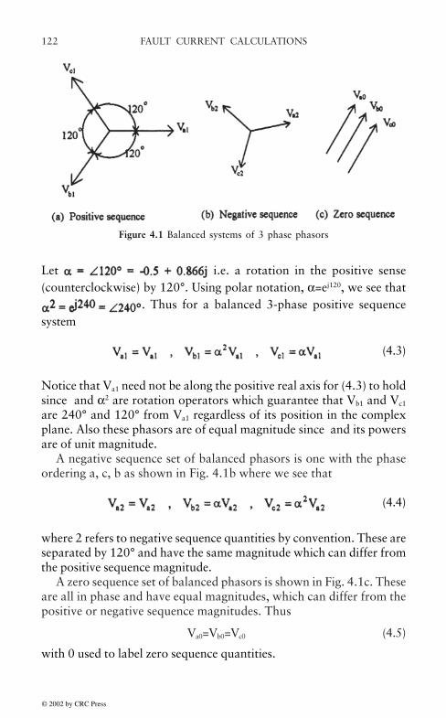
FAULT CURRENT CALCULATIONS122
Let i.e. a rotation in the positive sense(counterclockwise) by 120°. Using polar notation, α=ej120, we see that
. Thus for a balanced 3-phase positive sequencesystem
(4.3)
Notice that Va1 need not be along the positive real axis for (4.3) to holdsince and α2 are rotation operators which guarantee that Vb1 and Vc1
are 240° and 120° from Va1 regardless of its position in the complexplane. Also these phasors are of equal magnitude since and its powersare of unit magnitude.
A negative sequence set of balanced phasors is one with the phaseordering a, c, b as shown in Fig. 4.1b where we see that
(4.4)
where 2 refers to negative sequence quantities by convention. These areseparated by 120° and have the same magnitude which can differ fromthe positive sequence magnitude.
A zero sequence set of balanced phasors is shown in Fig. 4.1c. Theseare all in phase and have equal magnitudes, which can differ from thepositive or negative sequence magnitudes. Thus
Va0=Vb0=Vc0 (4.5)
with 0 used to label zero sequence quantities.
Figure 4.1 Balanced systems of 3 phase phasors
© 2002 by CRC Press

123FAULT CURRENT CALCULATIONS
We now show that it is possible to represent any unbalanced set of 3phasors by means of these balanced sequence sets. Let Va, Vb, Vc be suchan unbalance set as shown in Fig. 4.2. Since the positive, negative, andzero sequence balanced sets are determined once Va1, Va2, and Va0 arespecified, we need to find only these phase a components of thebalanced sets in terms of the original phasors to prove that thisrepresentation is possible. Write
(4.6)
Using (4.3), (4.4), and (4.5), this can be written
(4.7)
Figure 4.2 Unbalanced set of 3 phasors
© 2002 by CRC Press

FAULT CURRENT CALCULATIONS124
In matrix notation, we have
(4.8)
which is often abbreviated
Vabc=AV012 (4.9)
where Vabc and V012 are column vectors and A is the matrix in (4.8).Va0, Va1, Va2 can be found uniquely if A has an inverse. This can be
shown to be the case and the result is
(4.10)
as can be verified by direct computation, using the identities
1+α+α2=0α3=1α4=α (4.11)
Equation (4.10) can be abbreviated to
V012=A–1Vabc (4.12)
where A-1 is the matrix in (4.10) including the factor 1/3.Thus given any unbalanced set of phasors, the balanced positive,
negative, and zero sequence sets can be found or conversely, given thebalanced sets or just one phasor from each balanced set, chosencustomarily to be the a phasor, the unbalanced set can be obtained.
The virtue of this decomposition is that, using symmetricalcomponents, an unbalanced 3 phase system can be analyzed as 3 singlephase systems, each applying to one balanced sequence, in the samemanner that we need only consider one phase of a conventionalbalanced 3 phase system. However, the circuit model applying to each
© 2002 by CRC Press
125FAULT CURRENT CALCULATIONS
sequence may differ from the normal 3 balanced phases circuit model.This latter circuit model applies generally only to the positive sequence.The negative sequence circuit may differ from the positive, particularlyif there are generators or motors in the system. Not only can thepositive and negative impedances differ but, since generated voltagesare usually of positive sequence, voltage sources are absent from thenegative sequence circuit. For transformers, the impedances areindependent of phase order so that the positive and negative sequencecircuit models of transformers are identical.
The zero sequence circuit model can differ considerably from thepositive or negative one. For example, in a balanced 3-phase line, thecurrents add up to zero so there is no need for a return path or groundfor the currents to flow. Thus an effective ground point can be assumed.Since zero sequence currents are of equal magnitude and phase, theycannot sum to zero unless they are all zero. Thus for zero sequencecurrents to flow, a return path or ground is necessary. Thus in the zerosequence circuit model without ground or return path, an infiniteimpedance must be placed in the circuit.
In order to justify this approach, assume that the phase a, b, and c,circuits are identical as would be typical of a balanced 3-phase system.Let Via, Vib, Vic be corresponding branch voltages and Iia, Iib, Iic
corresponding branch currents for branch i in the phase a, b, and ccircuits. Then Kirchoff’s voltage and current laws can be expressed inthe form
where the Ki and Bi=± 1 or 0 and the column vector notation is employedso that each of the above vector equations represents 3 scalar equationswith the same Ki or Bi coefficients. Then multiplying on the left by A-1,these are transformed into
Thus we see that each set of sequence voltages or currents satisfies thesame Kirchoff equations. This means that the sequence networks behavelike ordinary electrical networks.
With regards to the circuit elements, the situation is a bit morecomplicated. Let the corresponding branch voltages and currents obeyan equation of the form, omitting the i subscript for simplicity,
© 2002 by CRC Press

FAULT CURRENT CALCULATIONS126
or, more compactly
Vabc=ZIabc
where Z is an impedance matrix. Then, pre-multiply by A-1 and,substituting V012=A-1 Vabc and Iabc=AI012, we get
V012=(A-1ZA)I012=ZseqI012
In general the sequence impedance matrix Zseq=A-1ZA which relates thesequence voltages and currents is not diagonal even if Z is. This meansthat there can be coupling between the different sequence circuits.
If the original circuit branches satisfy current-voltage relationshipsof the form
i.e. the corresponding branches have the same impedance and areuncoupled, then the sequence equations have the same form. This followssince the above Z matrix is a multiple of the identity and Zseq=ZaA--1
IA=ZaI reduces to the same multiple of the identity. In this example,there would be no need to use symmetrical components, since the originaluncoupled phase circuits could be solved with no more effort.
The method becomes more useful when, as is often the case inpractice, each sequence needs to be described by means of its own set ofsequence impedances, as for example when there is no return path forzero sequence currents. We assume these sequence impedances areuncoupled and equal for the 3 members of the balanced set. Thus, forthe positive sequence circuit we would have the branch currentrelationship,
© 2002 by CRC Press

127FAULT CURRENT CALCULATIONS
and similarly for the negative and zero sequences where Z2 and Z0
would be substituted for Z1 above. In this case, the sequence networkshave their own impedances and there is no coupling between sequences.In this case, the matrix Z connecting the branch phase quantities isnondiagonal in general. However, under normal operation with balancedpositive sequence voltages and currents, it reduces to the positive sequenceimpedance matrix shown above.
The fault analysis performed here assumes uncoupled sequencecircuits. We assume that the sequence impedances are known or can becalculated. For example, Z1 is taken to be the normal impedance topositive sequence current and for static devices such as transformers, Z2
=Z1. Z0 is more difficult to calculate, but can be measured by energizingthe 3 terminals of the device with voltages of the same phase.
4.3 FAULT ANALYSIS ON 3-PHASE SYSTEMS
We assume that the system is balanced before the fault occurs, that is,each phase has identical impedances and the currents and voltages arepositive sequence sets. Here we consider a general electrical system asshown in Fig. 4.3a. The fault occurs at some location on the systemwhere fault phase currents Ia, Ib, Ic flow. They are shown as leaving thesystem in the figure. The voltages to ground at the fault point are labeledVa, Vb, Vc. The system, as viewed from the fault point or terminal, ismodeled by means of Thevenin’s theorem. First, however, we resolvethe voltages and currents into symmetrical components so that we needonly analyze one phase of the positive, negative, and zero sequencesets. This is indicated in Fig. 4.3b where the a-phase sequence set hasbeen singled out.
© 2002 by CRC Press
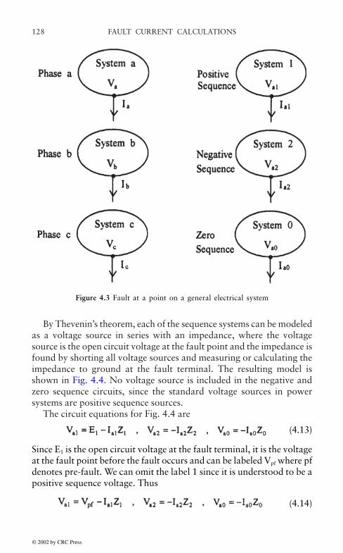
FAULT CURRENT CALCULATIONS128
By Thevenin’s theorem, each of the sequence systems can be modeledas a voltage source in series with an impedance, where the voltagesource is the open circuit voltage at the fault point and the impedance isfound by shorting all voltage sources and measuring or calculating theimpedance to ground at the fault terminal. The resulting model isshown in Fig. 4.4. No voltage source is included in the negative andzero sequence circuits, since the standard voltage sources in powersystems are positive sequence sources.
The circuit equations for Fig. 4.4 are
(4.13)
Since E1 is the open circuit voltage at the fault terminal, it is the voltageat the fault point before the fault occurs and can be labeled Vpf where pfdenotes pre-fault. We can omit the label 1 since it is understood to be apositive sequence voltage. Thus
Figure 4.3 Fault at a point on a general electrical system
(4.14)
© 2002 by CRC Press
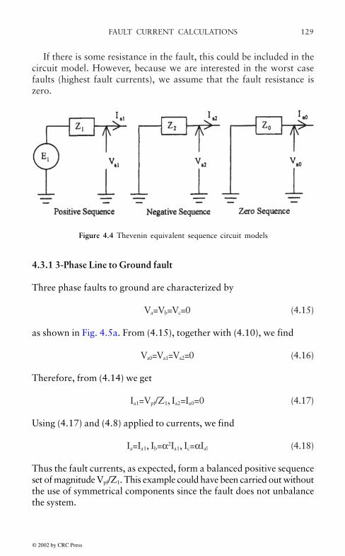
129FAULT CURRENT CALCULATIONS
4.3.1 3-Phase Line to Ground fault
Three phase faults to ground are characterized by
Va=Vb=Vc=0 (4.15)
as shown in Fig. 4.5a. From (4.15), together with (4.10), we find
Va0=Va1=Va2=0 (4.16)
Therefore, from (4.14) we get
Ia1=Vpf/Z1, Ia2=Ia0=0 (4.17)
Using (4.17) and (4.8) applied to currents, we find
Ia=Ia1, Ib=α2Ia1, Ic=αIal (4.18)
Thus the fault currents, as expected, form a balanced positive sequenceset of magnitude Vpf/Z1. This example could have been carried out withoutthe use of symmetrical components since the fault does not unbalancethe system.
Figure 4.4 Thevenin equivalent sequence circuit models
If there is some resistance in the fault, this could be included in thecircuit model. However, because we are interested in the worst casefaults (highest fault currents), we assume that the fault resistance iszero.
© 2002 by CRC Press

FAULT CURRENT CALCULATIONS130
4.3.2 Single Phase Line to Ground Fault
For a single phase to ground fault, we assume, without loss of generality,that the a-phase is faulted. Thus we have
(4.19)
as indicated in Fig. 4.5b. From (4.10) applied to currents, we get
Ia0=Ia1=Ia2=Ia/3 (4.20)
From (4.14), (4.19), and (4.20), we find
Va=0=Va0+Va1+Va2=Vpf–Ia1(Z1+Z2+Z0)
or
Figure 4.5 Standard fault types on 3 phase systems
© 2002 by CRC Press

131FAULT CURRENT CALCULATIONS
(4.21)
From (4.19) and (4.20), we get
(4.22)
4.3.3 Line to Line Fault
A line to line fault can, without loss of generality, be assumed to occurbetween lines b and c as shown in Fig. 4.5c. The fault equations are
(4.23)
From (4.10) applied to voltages and currents, we get
(4.24)
Using (4.14) and (4.24), we find
Va0=0, Va1-Va2=0=Vpf-Ia1(Z1+Z2)
or
(4.25)
Using (4.8) applied to currents, (4.24), and (4.25), we obtain
(4.26)
© 2002 by CRC Press

FAULT CURRENT CALCULATIONS132
4.3.4 Double Line to Ground Fault
The double line to ground fault, as shown in Fig. 4.5d, can be regardedas involving lines b and c. The fault equations are
Vb=Vc=0, Ia=0 (4.27)
From (4.27) and (4.10), we find
Va0=Va1=Va2=Va/3, Ia=Ia0+Ia1+Ia2=0 (4.28)
Using (4.14) and (4.28),
or
(4.29)
so that, from (4.14)
(4.30)
Substituting into (4.8) applied to currents, we obtain
© 2002 by CRC Press

133FAULT CURRENT CALCULATIONS
(4.31)
4.4 FAULT CURRENTS FOR TRANSFORMERS WITH 2 TERMINALSPER PHASE
A 2 terminal transformer can be modeled by a single leakage reactancewhich we call zHL where H and L indicate high and low voltage terminals.All electrical quantities from this point on will be taken to mean per-unit quantities and will be written with small letters. This will enable usto describe transformers, using a single circuit.
The high and low voltage systems external to the transformer aredescribed by system impedances zSH, zSL and voltage sources eSH, eSL.The resulting sequence circuit models are shown in Fig. 4.6. A zerosubscript is used to label the zero sequence circuit parameters since theycan differ considerably from the positive or negative sequence circuitparameters. The positive and negative circuit parameters are equal fortransformers and we will assume for the electrical systems also. Theybear no distinguishing subscript. We have shown a fault on the Hterminal in Fig. 4.6. By interchanging subscripts, the L terminal faultscan be obtained.
© 2002 by CRC Press
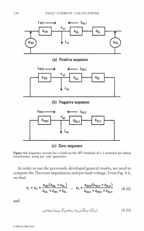
FAULT CURRENT CALCULATIONS134
In order to use the previously developed general results, we need tocompute the Thevenin impedances and pre-fault voltage. From Fig. 4.6,we find
(4.32)
and
Vpf=eSH-iSHpf ZSH=eSL-iHLpf(ZHL+ZSL) (4.33)
Figure 4.6 Sequence circuits for a fault on the HV terminal of a 2 terminal per phasetransformer, using per unit quantities
© 2002 by CRC Press

135FAULT CURRENT CALCULATIONS
where the pre-fault (pf) quantities are all positive sequence. Fig. 4.6 andthe above formulas assume that both terminals are connected to the HVand LV systems. If either terminal of the transformer is floating, thenthis is equivalent to setting the system impedance to infinity for thatsystem.
We are interested in obtaining the currents in the transformer duringthe fault. Thus, according to Fig. 4.6, we need to find iHL1, iHL2, iHL0 forthe standard faults. Since ia1, ia2, ia0 have already been obtained for thestandard faults, we must find the transformer currents in terms of theseknown fault currents. From Fig. 4.6 we see that
Va1=eSL-iHL1(ZHL+ZSL),Va2=-iHL2(ZHL+ZSL), Va0=-iHL0(ZHL0+ZSL0)
Using (4.33), we can rewrite this as
(4.34)
Naturally, if the transformer were not loaded before the fault, we wouldhave iHLpf=0. Substituting the per-unit version of (4.14) into (4.34), weobtain
4.4.1 3-Phase Line to Ground Fault
For this fault case, we substitute (4.17), expressed in per-unit terms,into (4.35) to obtain
(4.35)
(4.36)
© 2002 by CRC Press

FAULT CURRENT CALCULATIONS136
Then, using (4.8) applied to currents, we find
(4.37)
i.e. the fault currents in the transformer form a positive sequence set asexpected.
4.4.2 Single Phase Line to Ground Fault
For this type of fault, substitute the per-unit versions of (4.21) into (4.35),using z1=z2 to obtain
Substituting (4.38) into (4.8) applied to currents, we obtain the phasecurrents,
(4.38)
(4.39)
© 2002 by CRC Press

137FAULT CURRENT CALCULATIONS
Note that there is fault current in phases b and c inside the transformereven though the fault is on phase a. These b and c fault currents are oflower magnitude than the phase a fault current.
4.4.3 Line to Line Fault
For this type of fault, we substitute the per-unit versions of (4.25) into(4.35) using z1=z2, to obtain
(4.40)
Using (4.8) applied to currents, we obtain
(4.41)
In this case, with the fault between phases b and c, phase a is unaffected.
4.4.4 Double Line to Ground Fault
For this fault, we substitute (4.30) expressed in per-unit terms, into (4.35),using z1=z2, to obtain
(4.42)
© 2002 by CRC Press

FAULT CURRENT CALCULATIONS138
4.4.5 Zero Sequence Impedances
Zero sequence impedances require special consideration since certaintransformer 3-phase connections, such as the delta connection, blockthe flow of zero sequence currents and hence provide an essentiallyinfinite impedance to their passage. This is also true of the ungroundedY connection. The reason is that the zero sequence currents, being all inphase, require a return path in order to flow. The delta connectionprovides an internal path for the flow of these currents, circulating aroundthe delta, but blocks their flow through the external lines. Theseconsiderations do not apply to positive or negative sequence currentswhich sum to zero vectorially and so require no return path.
For transformers, since the amp-turns must be balanced for eachsequence, in order for zero sequence currents to be present, they mustflow in both windings. Thus in a grounded Y-Delta unit, for example,zero sequence currents can flow within the transformer but cannot flowin the external circuit connected to the delta side. Similarly, zerosequence currents cannot flow in either winding if one of them is anungrounded Y.
Fig. 4.7 shows some examples of zero sequence impedance diagramsfor different transformer connections. These should be compared withFig. 4.6c which applies to a grounded Y/grounded Y connection. Wherea break in a line occurs, imagine that an infinite impedance is inserted.Mathematically, one needs to let the impedance approach infinity as alimiting process in the formulas.
Using (4.8) applied to currents, we get for the phase currents
(4.43)
© 2002 by CRC Press

139FAULT CURRENT CALCULATIONS
For the Connection in Fig. 4.7a, the Thevenin impedance, looking infrom the fault point, is z0=zSH0 zHL0/(zSH0+zHL0) i.e. the parallelcombination of zSH0 and zHL0. In this case, the impedance zSL0 iseffectively removed from the circuit and replaced by zSL0=0. Thissubstitution should be made in all the formulas.
For the connection in Fig. 4.7b, we find z0=zSH0. In this case no zerosequence current can flow into the fault from the transformer side ofthe fault point so effectively zSL0→. Figs. 7c and 7d are similar.Because of the ungrounded Y connection, no zero sequence currentflows in the transformer.
Figure 4.7 Some examples of zero sequence impedance diagrams for 2 terminaltransformers. The arrow indicates the fault point. Yg=grounded Y, Yu= ungrounded Y
© 2002 by CRC Press

FAULT CURRENT CALCULATIONS140
Another issue is the value of the zero sequence impedancesthemselves when they are fully in the circuit. These values tend to differfrom the positive sequence impedances in transformers because themagnetic flux patterns associated with them can be quite different fromthe positive sequence flux distribution. This difference is taken intoaccount by multiplying factors which multiply the positive sequenceimpedances to produce the zero sequence values. For 3 phase core formtransformers, these multiplying factors tend to be ≈0.85, however theycan differ for different 3 phase connections and are usually found byexperimental measurements.
4.5 FAULT CURRENTS FOR TRANSFORMERS WITH 3 TERMINALSPER PHASE
A 3-terminal transformer can be represented in terms of 3 Y (or T)connected impedances if per-unit quantities are used. Fig. 4.8 shows thesequence circuits for such a transformer where H, X, Y label thetransformer impedances and SH, SX, SY label the associated systemimpedances. The systems are represented by impedances in series withvoltage sources. The positive sense of the currents is into the transformerterminals. Although the fault is shown on the H-terminal, byinterchanging subscripts, the formulas which follow can apply to faultsan any terminal. As before, we have not labeled the positive and negativesequence impedances with subscripts since they are equal for transformersand we assume also for the systems. The zero sequence impedances aredistinguished with subscripts because they can differ from their positivesequence counterparts.
© 2002 by CRC Press

141FAULT CURRENT CALCULATIONS
From Fig. 4.8, the Thevenin impedances, looking into the circuits fromthe fault point, are
Figure 4.8 Sequence circuits for a fault on the H terminal of a 3 terminal per phasetransformer, using per unit quantities
(4.44)
© 2002 by CRC Press

FAULT CURRENT CALCULATIONS142
The pre-fault voltage is given by
vpf=eSH-iSHpfzSH=eSX-iXpf(zX+zSX)+iHpfZH (4.45)=eSY-iYpf(zY+zSY)+iHpfzH
where pf labels pre-fault quantities which are all positive sequence. Wealso have
iH+iX+iY=0 (4.46)
which applies to the sequence and pre-fault currents. If a terminal isunloaded, then the corresponding pre-fault current should be set to zero.
From Fig. 4.8,
(4.48)
Solving (4.47), together with (4.44), (4.45), (4.46), and (4.14) expressedin per-unit terms, we obtain
(4.47)
© 2002 by CRC Press

143FAULT CURRENT CALCULATIONS
4.5.2 Single Phase Line to Ground Fault
For this fault, we substitute the per-unit version of (4.21) into (4.48),using z1=z2, to get
We now use these equations, together with the fault current equations toobtain the currents in the transformer for the various types of fault. Wewill only list the equations for the sequence currents. Equation (4.8),applied to currents, may be used to obtain the phase currents in terms ofthe sequence currents.
4.5.1 3-Phase line to ground fault
For this type of fault, we substitute the per-unit version of (4.17) into(4.48) to obtain
(4.49)
© 2002 by CRC Press
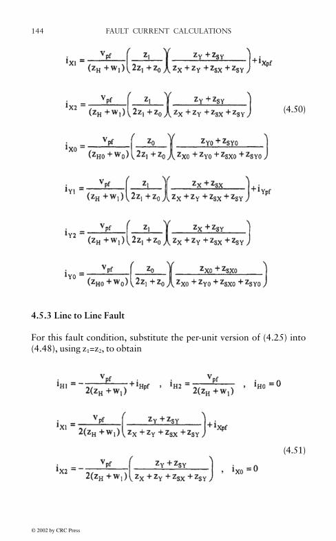
FAULT CURRENT CALCULATIONS144
4.5.3 Line to Line Fault
For this fault condition, substitute the per-unit version of (4.25) into(4.48), using z1=z2, to obtain
(4.50)
(4.51)
© 2002 by CRC Press

145FAULT CURRENT CALCULATIONS
4.5.4 Double Line to Ground Fault
For this fault, substitute the per-unit version of (4.30) into (4.48), usingz1=z2, to get
(4.52)
© 2002 by CRC Press

FAULT CURRENT CALCULATIONS146
4.5.5 Zero Sequence Impedances
Fig. 4.9 lists some examples of zero sequence circuits for 3-terminaltransformers. An infinite impedance is represented by a break in thecircuit. When substituting into the preceding formulas, a limiting processneeds to be used. Although there are many more possibilities than shownin Fig. 4.9, they can serve to illustrate the method for accounting for thedifferent 3-phase connections. The previous formulas apply directly toFig. 4.8c which represents a transformer with all grounded Y terminalconnections.
Figure 4.9 Some examples of zero sequence circuit diagrams for 3 terminal transformers.The arrow indicates the fault point. Yg=grounded Y, Yu= ungrounded Y
© 2002 by CRC Press
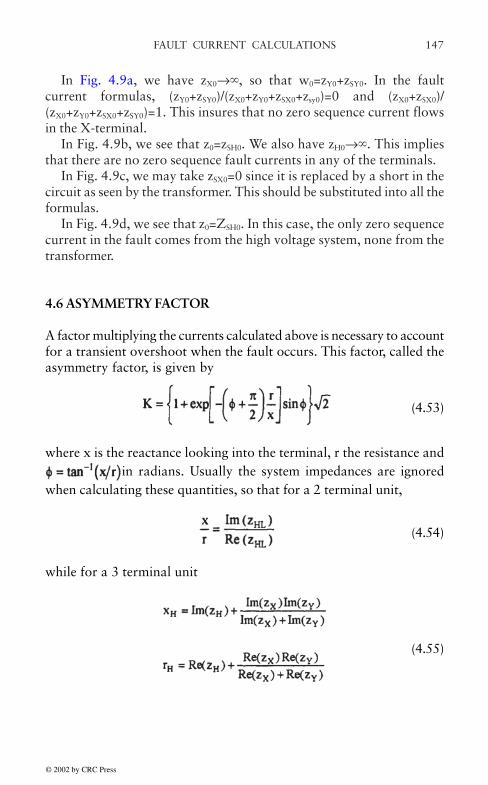
147FAULT CURRENT CALCULATIONS
In Fig. 4.9a, we have zX0→, so that w0=zY0+zSY0. In the faultcurrent formulas, (zY0+zSY0)/(zX0+zY0+zSX0+zsy0)=0 and (zX0+zSX0)/(zX0+zY0+zSX0+zSY0)=1. This insures that no zero sequence current flowsin the X-terminal.
In Fig. 4.9b, we see that z0=zSH0. We also have zH0→. This impliesthat there are no zero sequence fault currents in any of the terminals.
In Fig. 4.9c, we may take zSX0=0 since it is replaced by a short in thecircuit as seen by the transformer. This should be substituted into all theformulas.
In Fig. 4.9d, we see that z0=ZSH0. In this case, the only zero sequencecurrent in the fault comes from the high voltage system, none from thetransformer.
4.6 ASYMMETRY FACTOR
A factor multiplying the currents calculated above is necessary to accountfor a transient overshoot when the fault occurs. This factor, called theasymmetry factor, is given by
(4.53)
where x is the reactance looking into the terminal, r the resistance andin radians. Usually the system impedances are ignored
when calculating these quantities, so that for a 2 terminal unit,
(4.54)
while for a 3 terminal unit
(4.55)
© 2002 by CRC Press

FAULT CURRENT CALCULATIONS148
with corresponding expressions for xX, rX , xY, rY. When K in (4.53)multiplies the rms short circuit current, it yields the maximum peakshort circuit current.
© 2002 by CRC Press

149
5. RABINS’ METHOD FORCALCULATING LEAKAGE FIELDS,FORCES, AND INDUCTANCES IN
TRANSFORMERS
Summary Rabin’s method utilizes a simplified transformer geometry,consisting of a core, coils, and yokes of infinite extent, to solve Maxwell’sequations. This method works well for calculating the magnetic fieldnear the coils so that quantities such as inductances and forces whichdepend on this near field are accurately calculated. Since the tank wall,clamping structure, and other details are omitted, this method does notallow one to calculate stray losses in these structures. We use this methodto find forces, the two winding leakage inductance, as well as self andmutual inductances between coil sections.
5.1 INTRODUCTION
Modern general purpose computer programs are available for calculatingthe magnetic field inside the complex geometry of a transformer. Thesenumerical methods generally employ finite elements or boundaryelements. Geometric details such as the tank wall and clamping structurecan be included. While 3D programs are available, 2D programs usingan axisymmetric geometry are adequate for most purposes. Althoughinputting the geometiy, the Ampere-turns in the winding sections, andthe boundary conditions can be tedious, parametric procedures are oftenavailable for simplifying this task. Along with the magnetic field,associated quantities such as inductances and forces can be calculatedby these methods. In addition, eddy currents in structural parts and theiraccompanying losses can be obtained with the appropriate a.c. solver.
In spite of these modern advances in computational methods, olderprocedures can often be profitably employed to obtain quantities ofinterest very quickly and with a minimum of input. One of these isRabins’ method, which assumes an idealized transformer geometiy[Rab56]. This simplified geometry permits analytic formulas to be
© 2002 by CRC Press
RABINS’ METHOD150
developed for the magnetic field and other useful quantities. Thegeometry consists of a single leg of a single or possibly 3 phasetransformer. The leg consists of a core and surrounding coils which areassumed to be axisymmetric, along with yokes which are assumed to beof infinite extent at the top and bottom of the leg. The entireaxisymmetric geometry is of infinite extent radially. Thus there are notank walls or clamping structures in the geometry. In addition, the coreand yokes are assumed to be infinitely permeable.
In spite of these simplifications, Rabins’ method does a good job ofcalculating the magnetic field in the immediate vicinity of thewindings. Thus forces and inductances, which depend largely on thefield-near the windings, are also accurately obtained. This can beshown by direct comparison with a finite element solution applied to amore complex geometry, including tank wall and clamps. Although thefinite element procedure can obtain losses in structural parts, Rabins’method is not suited for this. However, because the magnetic field nearor inside the windings is obtained accurately, eddy current losses in thewindings as well as their spatial distribution can be accurately obtainedfrom formulas based on this leakage field.
In the following, we present Rabins’ method and show how it can beused to obtain forces, leakage reactances, and self and mutualinductances between winding sections for use in detailed circuit modelsof transformers such as are needed in impulse calculations.
5.2 THEORY
We model a cylindrical coil or section of a coil surrounding a core legwith top and bottom yokes as shown in Fig. 5.1. The yokes and core arereally boundaries of the geometry which extends infinitely far radially.The coils are assumed to be composed of stranded conductors so that noeddy current effects are modeled. Thus we can assume d.c. conditions,The current density in the coil is assumed to be piecewise constant axiallyand uniform radially as shown in Fig. 5.2. As indicated, there can beregions within the coil where the current density drops to zero. Sincethere are no non-linear effects within the geometry modeled, the fieldsfrom several coils can be added vectorially so that it is only necessaryto model one coil at a time.
© 2002 by CRC Press

RABINS’ METHOD 151
Figure 5.1 Geometry of iron core, yokes, and coil or coil section
Figure 5.2 Axial distribution of current density in the coil
© 2002 by CRC Press

RABINS’ METHOD152
Maxwell’s equations for the magnetic field, applied to the geometryoutside the core and yokes and assuming static conditions are, in SI units,
(5.1)
(5.2)
where H is the magnetic field, B the induction, and J the current density.Defining a vector potential A, by
(5.3)
equation (5.2) is automatically satisfied. We also have
B=µoH (5.4)
in the region of interest where µo is the permeability of vacuum, oil, orair. Substituting (5.3) and (5.4) into (5.1), we obtain
(5.5)
The vector potential is not completely defined by (5.3). It contains somearbitrariness which can be removed by setting
(5.6)
Thus (5.5) becomes
(5.7)
The current density vector is azimuthal so that
(5.8)
where aϕ is the unit vector in the azimuthal direction. Because of theaxisymmetric geometiy, all the field quantities are independent of ϕ.With these assumptions (5.7) becomes in cylindrical coordinates
(5.9)
© 2002 by CRC Press

RABINS’ METHOD 153
Thus A and J have only a ϕ component and we drop this subscript in thefollowing for simplicity.
Let us write the current density as a Fourier series in terms of afundamental spatial period of length L, the yoke to yoke distance orwindow height.
(5.10)
where
(5.11)
For the current density described in Fig. 5.2, we have
(5.12)
Using (5.12), the integrals in (5.11) can be evaluated to get
(5.13)
Thus for one section with constant current density J we would have
© 2002 by CRC Press

RABINS’ METHOD154
(5.14)
As shown in Fig. 5.1, we have divided the solution space into 3regions:
In regions I and III, the current density is 0 so equation (5.9) becomes,dropping the subscript ϕ
(5.15)
This is a homogeneous partial differential equation. We look for asolution of the form
A(r,z)=R(r)Z(z) (5.16)
Substituting this into (5.15) and dividing by RZ, we get
(5.17)
This equation contains terms which are only a function of r and termswhich are only a function of z whose sum is a constant=0. Therefore,each set of terms must separately equal a constant whose sum is zero.Let the constant be m2, a positive number. Then
(5.18)
Rearranging terms, we get
© 2002 by CRC Press

RABINS’ METHOD 155
(5.19)
We need to consider separately the cases m=0 and m>0.For m=0, the solution to the z equation which satisfies the boundary
conditions at the top and bottom yokes is a constant and the r equationin (5.19) becomes
(5.20)
The solution to this equation is
(5.21)
where S and T are constants to be determined by the boundaryconditions,
For m>0, the solution to the z equation in (5.19) can be written
(5.22)
where Zm and ϕm are constants to be determined by the boundaryconditions. Since we assume that the yoke material has infinitepermeability, this requires that the B-field be perpendicular to the yokesurfaces. Using (5.3), we have in cylindrical coordinates
(5.23)
where ar and k are unit vectors in the r and z directions. For B to beperpendicular to the upper and lower yokes, we must have
(5.24)
Using this, (5.22) takes the form
(5.25)
© 2002 by CRC Press
RABINS’ METHOD156
Here we use n rather than m to label the constant. m also depends on nbut we omit this reference for simplicity.
For m>0, the radial equation in (5.19) can be written, with thesubstitution x=mr,
(5.26)
The solution to this equation is
Rn=CnI1+DnK1(x) (5.27)
where I1 and K1 are modified Bessel functions of the first and secondkind respectively and of order 1 [Dwi61]. We have also labeled theconstants C and D with the subscript n since the solution depends on nthrough m which occurs in x.
In general, the solution to (5.15) is expressible as a sum of theseindividual solutions, each a product of an R and Z term,
(5.28)
where the Z solution constants have been absorbed in the overall constantsshown. This solution satisfies the boundary condition at z=0, L. Becausewe also assume an infinitely permeable core, the B-field must be normalto the core surface. Thus from (5.23), we require in Region I
(5.29)
Substituting (5.28) into this last equation, we get
(5.30)
Although (5.30) would seem to require that S=0, it will turn out thatwhen all the windings are considered with their Ampere-turns which
© 2002 by CRC Press

RABINS’ METHOD 157
sum to zero, we can satisfy this boundary condition with S≠0 for eachwinding. For the remaining z-dependent terms in (5.30), we require
(5.31)
where we have used modified Bessel function identities [Rab56]. I0 andK0 are modified Bessel functions of order 0. Thus we have from (5.31)
(5.32)
Labeling the unknown constants with the region number assuperscript, (5.28) becomes
(5.33)
We have dropped the T/r term since it approaches infinity as the coreradius approaches zero. We also assume implicitly that m depends on nas in (5.28).
In Region III, we require that A be finite as r→∞. Since I1→∞ as r→∞and the Sr term also →∞, we have from (5.28), using the appropriateregion label,
(5.34)
In Region II, we must keep the current density term in (5.9).Substituting the Fourier series (5.10) into (5.9) and dropping the ϕsubscript, we have in Region II,
(5.35)
We look for a solution to this equation in the form of a series expansion,
© 2002 by CRC Press

RABINS’ METHOD158
(5.36)
Substituting into (5.35), we get
(5.37)
Since the cosine functions are orthogonal, we can equate correspondingcoefficients on both sides of this equation. We obtain
(5.38)
The soludon to the n=0 equation can be written in terms of a solutionof the homogeneous equation plus a particular solution,
(5.39)
The solution to the n>0 equations in (5.38) consists of a homogeneoussolution which was found previously and a particular solution,
(5.40)
where L1 is a modified Struve function of order 1 [Abr72]. Thus thesolution (5.36) is given explicitly as
(5.41)
© 2002 by CRC Press

RABINS’ METHOD 159
This equation already satisfies the boundary conditions at z=0, L.The unknown constants must be determined by satisfying the boundaryconditions ar r=r1, r2. We require that the vector potential be continuousacross the interfaces. Otherwise the B-field given by (5.23) wouldcontain infinities. Thus at r=r1, using (5.33) and (5.41),
(5.42)
Since this must be satisfied for all z, we obtain
(5.43)
where x1=mr1, xc=mrc.At r=r2, we obtain similarly, using (5.34) and (5.41),
(5.44)
where x2=mr2.In addition to the continuity of A at the interfaces between regions,
we also require, according to Maxwell’s equations, that the normalcomponent of B and the tangential component of H be continuousacross these interfaces. According to (5.23), the normal B componentsare already continuous across these interfaces since all regional
© 2002 by CRC Press

RABINS’ METHOD160
solutions have the same z dependence and because the A’s arecontinuous. Since B is proportional to H in all regions of interest here,we require that the tangential B components be continuous. Thus from(5.23), we require that
(5.45)
be continuous at r=r1, r2 (x=x1, x2). Using this, we obtain the additionalconditions on the unknown constants
(5.46)
Using the identities [Rab56, Abr72],
(5.47)
we obtain for the last two equations in (5.46)
(5.48)
© 2002 by CRC Press

RABINS’ METHOD 161
Solving for the S and T constants from (5.43), (5.44), and (5.46), weobtain
(5.49)
Solving for the Cn and Dn constants from (5.43), (5.44), and (5.46), weget
(5.50)
Using the identities [Rab56],
(5.51)
© 2002 by CRC Press

RABINS’ METHOD162
we can transform (5.50) into the form
(5.52)
Summarizing and simplifying the notation slightly, the solutions inthe three regions are given by
(5.53)
where m=nπ/L, x=mr, and
© 2002 by CRC Press
RABINS’ METHOD 163
(5.54)
Here x1=mr1 and x2=mr2.Note that, using (5.23), the axial component of the induction vector
at the core radius is
Bz(rc,z)=µoJ0(r2-r1) (5.55)
This is µo times the average current density times the radial build of thewinding. Since the axial height L is the same for all the windings, whenwe add this axial component for all the windings we will get zero, assumingAmpere-turn balance. Thus the flux will enter the core radially as required.
Although the modified Bessel functions are generally available inmathematical computer libraries, the modified Struve functions are notso easily obtained. We therefore indicate here some methods ofobtaining these and other quantities of interest in terms of readilyavailable functions or easily evaluated integrals. From reference[Abr72], the modified Struve functions are given in integral form as
(5.56)
It can be seen from (5.56) that these functions become asymptoticallylarge as x→∞. Such large values of x would occur when evaluating the
© 2002 by CRC Press

RABINS’ METHOD164
higher harmonics in (5.53). Ref. [Abr72] also gives integral expressionsfor the modified Bessel functions. In particular, we have
(5.57)
These also become asymptotically large as x increases. However, bydefining the difference functions
(5.58)
we can show that
(5.59)
The integrals in (5.59) are well behaved as x increases and can beevaluated numerically. In subsequent developments, we will also needthe integral of M0. This is readily determined from (5.59) as
(5.60)
The integrand approaches x as θ→π/2 and so the integral is also wellbehaved. For high x values, asymptotic series can be found in Ref.[Abr72].
Let us now write other expressions of interest in terms of the Mfunctions and modified Bessel functions. Using (5.51) and (5.58), we canwrite
(5.61)
© 2002 by CRC Press

RABINS’ METHOD 165
We will also need a similar integral for the modified Struve function.We need the following identities given in [Rab56].
(5.62)
Multiplying these by t and integrating from 0 to x, we get
(5.63)
Substituting L0 in terms of the M0 function and rearranging, we get
(5.64)
Thus all the functions needed to determine the vector potential areobtainable in terms of the modified Bessel functions and the M functions.We will also need (5.64) in obtaining derived quantities in the followingsections.
The determination of the vector potential for the other coils or coilsections proceeds identically to the previous development. BecauseMaxwell’s equations are linear in the fields and potentials in the regionoutside the core and yokes, we can simply add the potentials or fieldsfrom the various coils vectorially at each point to get the net potentialor field. We need to be aware of the fact that a given point may not bein the same region number (I, II, or III) for the different coils.
© 2002 by CRC Press

RABINS’ METHOD166
5.3 DETERMINING THE B-FIELD
The B-field or induction vector is given by (5.23). We need to evaluateit in the three regions using (5.53). The radial component is, using theregion label as superscript,
(5.65)
Using (5.47) and
(5.66)
the axial component is,
(5.67)
To find the net B-field associated with a collection of coils, we simplyadd their components at the point in question, keeping in mind whatregion the point is in relative to each coil.
© 2002 by CRC Press

RABINS’ METHOD 167
5.4 DETERMINING THE WINDING FORCES
The force density vector, F, in SI units (Newtons/m3), is given by
F=J×B (5.68)
Since J is azimuthal and B has only r and z components, this reduces to
F=JBzar-JBrk (5.69)
where ar is the unit vector in the radial direction and k the unit axialvector. We have omitted the ϕ subscript on J. Thus the radial forces aredue to the axial field component and vice versa.
In (5.69), the B-field values are the resultant from all the coils and Jis the current density at the point in question. This force density isnonzero only over those parts of the winding which carry current. Inorder to obtain net forces over all or part of a winding, it is necessary tointegrate (5.69) over the winding or winding part. For this purpose, thewinding can be subdivided into as fine a mesh as desired and Fcomputed at the centroids of these subdivisions and the resulting valuestimes the mesh volume element added.
One force which is useful to know is the compressive force whichacts axially at each axial position in the winding. We assume that thewindings are constrained at the two ends by pressure rings of some type.We ignore gravity here. Starting from the bottom, we integrate theaxial forces upwards along the winding, stopping when the sum of thedownward acting forces reach a maximum. This is the net downwardforce on the bottom pressure ring which is countered by an equalupward force on the winding exerted by the pressure ring. We do thesame thing, starting from the top of the winding, integrating the axialforces until the largest upwards acting summed force is reached. Thisthen constitutes the net upward force acting on the top pressure ringwhich is countered by an equal downward force exerted by the pressurering. Including the reaction forces of the pressure rings, we thenintegrate upwards say, starting at the bottom of the winding and at eachvertical position, the force calculated will be the compressive force atthat position since there will be an equal and opposite force acting fromabove. This is illustrated in Fig. 5.3a.
© 2002 by CRC Press

RABINS’ METHOD168
Another force of interest for coil design is the radial force whichresults in hoop stress, tensile or compressive, on the winding. Because ofthe cylindrical symmetry, the radial forces vectorially add to zero. Wemust therefore handle them a bit differently if we are to arrive at auseful resultant for hoop stress calculations. In Fig. 5.3b, we isolate asmall portion of the winding and show the forces acting in a horizontalsection. We show the radial forces acting outward and the tensile forcesapplied by the missing part of the winding which are necessary tomaintain equilibrium. If the radial forces acted inward, then the rest ofthe winding would need to apply compressive forces to maintainequilibrium and all the force arrows in the figure would be reversed.The calculation would, however, proceed similarly.
In Fig. 5.3b, θ is assumed to be a very small angle. The force balancein the upward direction in the figure is
(5.70)
Ftot, r is the sum of the radial electromagnetic forces acting on the windingsection shown and T is the total tensile force acting on the windingcross-section. For small θ, this reduces to
Ftot, r=Tθ (5.71)
Figure 5.3 Forces on the winding needed for stress analysis
© 2002 by CRC Press
RABINS’ METHOD 169
In radians, θ=∆/R, where ∆ is the circumferential length of the windingsection shown and R its average radius. The average tensile stress isσ=T/A, where A is the cross-sectional area of the winding section. Notingthat the volume of the winding section is ∆V=A ∆. In the limit of smallθ, (5.71) becomes
(5.72)
Thus the average tensile stress in the winding is the average radiustimes the average radial force density, assuming the radial forces actoutward. For inward radial forces, σ is compressive. The average radialforce density at a particular axial position z can be found by computingthe radial component of (5.69) at several radial positions in the winding,keeping z fixed, and taking their average. One should weight these bythe volume element which is proportional to r.
Other forces of interest can be found from the known forcedensities.
5.5 GENERAL METHOD FOR DETERMINING INDUCTANCESAND MUTUAL INDUCTANCES
Self and leakage inductances are usually defined in terms of flux linkagesbetween circuits. However, it is often more convenient to calculatethem in terms of magnetic energy. In this section, we show theequivalence of these methods and develop a useful formula for thedetermination of these inductances in terms of the vector potential. Inaddition, we show how the vector potential can be employed tocalculate mutual inductances.
Consider a set of stationary circuits as shown in Fig. 5.4a. Weassume that we slowly increase the currents in them by means ofbatteries with variable control. In calculating the work done by thebatteries, we ignore any I2R or dissipative losses or, more realistically,we treat these separately. Thus the work we are interested in is the worknecessary to establish the magnetic field. Because of the changing fluxlinking the different circuits, emf’s s will be induced in them byFaraday’s law. We assume that the battery controllers are adjusted sothat the battery voltages just balance the induced voltages throughoutthe process. Because the circuits can have finite cross sectional areas as
© 2002 by CRC Press
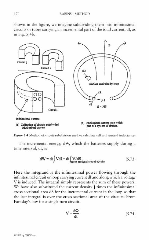
RABINS’ METHOD170
shown in the figure, we imagine subdividing them into infinitesimalcircuits or tubes carrying an incremental part of the total current, dI, asin Fig. 5.4b.
Figure 5.4 Method of circuit subdivision used to calculate self and mutual inductances
The incremental energy, dW, which the batteries supply during atime interval, dt, is
(5.73)
Here the integrand is the infinitesimal power flowing through theinfinitesimal circuit or loop carrying current dI and along which a voltageV is induced. The integral simply represents the sum of these powers.We have also substituted the current density J times the infinitesimalcross-sectional area dS for the incremental current in the loop so thatthe last integral is over the cross-sectional area of the circuits. FromFaraday’s law for a single turn circuit
(5.74)
© 2002 by CRC Press

RABINS’ METHOD 171
where Φ is the flux linked by the circuit. Substituting into (5.73)
(5.75)
By definition
(5.76)
In (5.76), the surface integral is over the surface encircled by the loopand the line integral is along the loop as shown in Fig. 5.4b. n is the unitnormal to the surface encircled by the loop and d is the infinitesimaldistance vector along the loop. Note that d points in the same directionas J considered as a vector. Since the current loops are fixed, we getfrom (5.76)
(5.77)
Substituting this into (5.75), we get
(5.78)
Since J points along d and since the volume element dV=ddS, we canrewrite (5.78)
(5.79)
In changing to a volume integral, we are simply recognizing the factthat the integral over the cross-sectional area of the circuits combinedwith an integral along the lengths of the infinitesimal circuits amountsto an integration over the volume of the circuits. If A increases linearlywith J, it can be shown that the total work done to establish the finalfield values is
© 2002 by CRC Press

RABINS’ METHOD172
(5.80)
It is sometimes more convenient for calculational purposes to express(5.80), or more generally (5.79), differently. First of all the volumeintegration in both of these equations could be taken over all spacesince the current density is zero everywhere except within the circuits.(By all space we mean the solution space of the problem of interest,ignoring the rest of the universe.) Substituting (5.1) into (5.79), we get
(5.81)
Using the vector identity for general vector fields P, Q [Pug62],
(5.82)
we have, upon substitution into (5.81) with the identification P→H, Q→dA,
(5.83)
In this equation, we have used the definition of A given in (5.3) and theDivergence Theorem [Pug62] to convert the last volume integral into asurface integral. The surface integral generally vanishes since theboundary surface is usually at infinity where the fields drop to zero. Inthe case of Rabins’ solution, it also vanishes on the core and yoke surfacesbecause of the boundary conditions. Thus we can drop it, to get for thesituation where B increases linearly with H
(5.84)
Either (5.80) or (5.84) can be used to calculate the magnetic energy. Thesecond equality in both equations applies to linear systems.
© 2002 by CRC Press

RABINS’ METHOD 173
We now show how the magnetic energy can be related to inductancesor leakage inductances. The voltages induced in the circuits of Fig. 5.4acan be written in terms of inductances and mutual inductances as
(5.85)
where Mij is the mutual inductance between circuits i and j. When j= i,Mii=Li, where Li is the self inductance of circuit i. The incremental energyfor the circuits of Fig. 5.4a can be expressed, using (5.85),
(5.86)
For linear systems, it can be shown that Mij=Mji. Thus the second sum in(5.86) can be written
(5.87)
The first equality in this equation is a matter of changing the indexlabels in the sum and the second equality results from the symmetricnature of Mij. The third equality results from the double counting whichhappens when i and j are summed independently. Substituting (5.87)into (5.86), we get
(5.88)
Integrating this last equation, we obtain
(5.89)
© 2002 by CRC Press
RABINS’ METHOD174
Thus (5.89) is another expression for the magnetic energy in terms ofinductances and mutual inductances. As an example, consider a singlecircuit for which we want to know the self-inductance. From (5.89),
(5.90)
where W can be calculated from (5.80) or (5.84) with only the singlecircuit in the geometry. W is usually available from finite element codes.If we have 2 circuits, then (5.89) becomes
(5.91)
If these two circuits are the high (label 1) and low (label 2) voltagecoils of a 2 winding transformer with N1 and N2 turns respectively,then we have I2/I1=”N1/N2 so that (5.91) becomes
(5.92)
The expression on the left is the leakage inductance referred to the highvoltage side [MIT43]. The magnetic energy on the right side can becalculated from (5.80) or (5.84) with the two windings in the geometryand with the Ampere-turns balanced. Multiplying by ω=2πf producesthe leakage impedance.
The mutual inductance between two circuits is needed in detailedcircuit models of transformers where the circuits of interest are sectionsof the same or different coils. We can obtain these quantities in terms ofthe vector potential. By definition, the mutual inductance betweencircuits 1 and 2, M12, is the flux produced by circuit 2 which linkscircuit 1 divided by the current in circuit 2. 1 and 2 could beinterchanged in this definition without changing the value of the mutualinductance for linear systems. We use the infinitesimal loop approachas illustrated in Fig. 5.4 to obtain this quantity. Each infinitesimal looprepresents an infinitesimal fraction of a turn. For circuit 1, aninfinitesimal loop carrying current dIi represents a fractional turn dI1/ I1.Therefore the flux linkage between this infinitesimal turn due to the fluxproduced by circuit 2, dλ12, is
© 2002 by CRC Press

RABINS’ METHOD 175
(5.93)
Integrating this expression over the cross-sectional area of circuit 1 andusing the fact that dI1=J1dS1 and that J1 as a vector points along d1, wecan write
(5.94)
where we have used the same integration devices as were used previously.Thus the mutual inductance between these circuits is given by
(5.95)
Note that this formula reduces to the formula for self-inductance (5.90)when 1 and 2 are the same circuit and letting M11=L1.
5.6 RABINS’ FORMULA FOR LEAKAGE REACTANCE
The leakage reactance for a 2 winding transformer as given in (5.92)can be obtained from the total magnetic energy. We assume that the twowindings occupy different radial positions as shown in Fig. 5.5. We use(5.80) for the magnetic energy where A is the total vector potential dueto both windings. Since A and J are both azimuthally directed, the dotproduct becomes simply the ordinary product. We also drop the impliedsubscript on J and A.
© 2002 by CRC Press
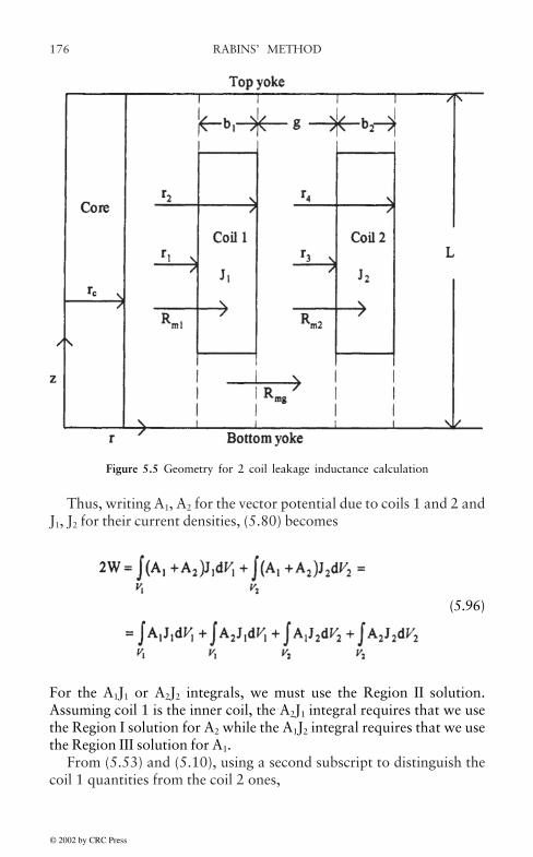
RABINS’ METHOD176
Thus, writing A1, A2 for the vector potential due to coils 1 and 2 andJ1, J2 for their current densities, (5.80) becomes
(5.96)
For the A1J1 or A2J2 integrals, we must use the Region II solution.Assuming coil 1 is the inner coil, the A2J1 integral requires that we usethe Region I solution for A2 while the A1J2 integral requires that we usethe Region III solution for A1.
From (5.53) and (5.10), using a second subscript to distinguish thecoil 1 quantities from the coil 2 ones,
Figure 5.5 Geometry for 2 coil leakage inductance calculation
© 2002 by CRC Press

RABINS’ METHOD 177
(5.97)
Performing the z-integral first, we notice that product terms whichcontain a single cosine term will vanish, i.e.
(5.98)
Product terms which contain 2 cosine factors have the value
(5.99)
After performing the z-integral, (5.97) becomes
(5.100)
Performing the r-integration, we get
© 2002 by CRC Press
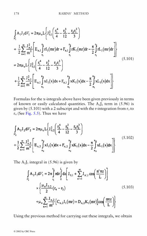
RABINS’ METHOD178
(5.101)
Formulas for the x-integrals above have been given previously in termsof known or easily calculated quantities. The A2J2 term in (5.96) isgiven by (5.101) with a 2 subscript and with the r-integration from r3 tor4 (See Fig. 5.5). Thus we have
(5.102)
The A2J1 integral in (5.96) is given by
(5.103)
Using the previous method for carrying out these integrals, we obtain
© 2002 by CRC Press

RABINS’ METHOD 179
(5.104)
The A1J2 integral in (5.96) is given similarly by
(5.105)
In spite of their different appearances, (5.104) and (5.105) are the same.Summing up the terms in (5.96), we get after some algebraic manipulation
(5.106)
When the coefficients En and Fn etc. have a 1 subscript, then theexpressions given by (5.54) apply with x1, x2 for the integration limits.However, when the second subscript is a 2, then x3, x4 must be substitutedfor x1, x2 in the formulas.
The first set of terms involving the J0's can be further manipulated byrealizing that the average current density in the coil times the area ofthe coil equals the total Ampere-turns in the coil so that
(5.107)
© 2002 by CRC Press

RABINS’ METHOD180
Using this and the geometric parameters shown in Fig. 5.5, this set ofterms can be expressed as
(5.108)
where Rm1, Rm2 are the mean radii of the coils, b1, b2 their radialthicknesses, Rmg is the mean radius of the gap, and g the gap’s radialthickness. In this equation NI could refer to either coil since they areequal except for sign.
The leakage inductance, referred to coil 1 as given in (5.92), can bewritten, using (5.106) and (5.108),
(5.109)
The first set of terms in this last equation is the leakage inductanceproduced by the axial flux from two coils with uniformly distributedcurrents and no end effects. The second set of terms has been written interms of NI to emphasize that it, along with N could refer to either coil.To get the leakage impedance multiply Lleak by ω=2πf.
There are sometimes transformer designs where two coils are placedon top of each other axially and therefore occupy the same radialposition. In this case the coil radial builds are usually the same. Often thecoils are duplicates. Rabins’ method can also be used to find the leakageinductance for this situation. The current densities for each coil will benon-zero within different axial regions but the Fourier decompositionshould reflect this. In this case, only the region II solution is needed forboth coils and (5.96) still holds. In this case, r3=r1 and r4=r2. Evaluatingthe terms in (5.96), we find that the A1J1 and A2J2 terms are the same asbefore except that we must replace r3, r4, x3, x4 by r1, r2, x1, x2.
The A2J1 integral is
© 2002 by CRC Press
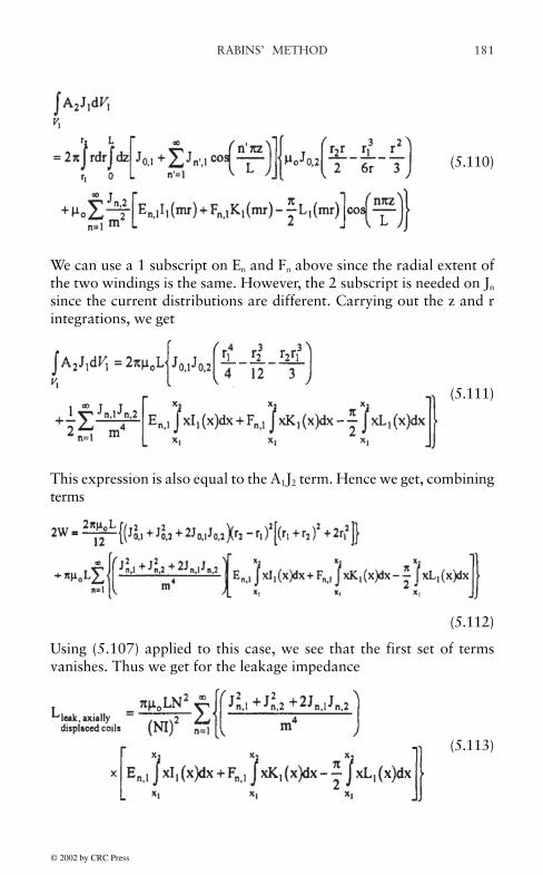
RABINS’ METHOD 181
(5.110)
We can use a 1 subscript on En and Fn above since the radial extent ofthe two windings is the same. However, the 2 subscript is needed on Jn
since the current distributions are different. Carrying out the z and rintegrations, we get
(5.111)
This expression is also equal to the A1J2 term. Hence we get, combiningterms
(5.112)
Using (5.107) applied to this case, we see that the first set of termsvanishes. Thus we get for the leakage impedance
(5.113)
© 2002 by CRC Press

RABINS’ METHOD182
5.7 RABINS’ METHOD APPLIED TO CALCULATE SELF ANDMUTUAL INDUCTANCES OF COIL SECTIONS
A coil section for our purposes here consists of a part of a coil which hasa uniform current density. Then (5.14) holds for the Fourier coefficients.In all other respects it is treated like a full coil. The self-inductance ofthis section is given by (5.95) with the subscript 2 replaced by 1. In thiscase, we use the solution for A in Region II since that is where thecurrent density is non-zero. The integral in (5.95) has already beencarried out in (5.101) so we have
(5.114)
Since
(5.115)
we can rewrite (5.114)
(5.116)
The mutual induction between two coil sections is given by (5.95). Hereagain, except for the uniform current density in one coil section, wetreat the coil sections as if they were full coils in applying Rabins’method. If the sections are on the same coil or two coils axially displaced,then A2 is the solution in Region II. The A2J1 integral has already beendone in this case and is given in (5.111). Thus we have
© 2002 by CRC Press
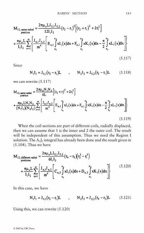
RABINS’ METHOD 183
(5.117)
Since
(5.118)
we can rewrite (5.117)
(5.119)
When the coil sections are part of different coils, radially displaced,then we can assume that 1 is the inner and 2 the outer coil. The resultwill be independent of this assumption. Thus we need the Region Isolution. The A1J2 integral has already been done and the result given in(5.104). Thus we have
(5.120)
In this case, we have
(5.121)
Using this, we can rewrite (5.120)
© 2002 by CRC Press

RABINS’ METHOD184
(5.122)
From the formulas for leakage, self, and mutual inductances, we seethat all the results can be expressed in terms of the modified Besselfunctions of order 0 and 1, the M0, M1 functions, and the integral of theM0 function. The M0, M1 and the integral of the M0 function haveconvenient expressions in terms of well behaved integrals.
© 2002 by CRC Press

185
6. MECHANICAL DESIGN
Summary During fault conditions when currents can increase to about25 times their normal values, transformer windings are subjected tovery high forces. Sufficient bracing must be provided so that littlemovement occurs. In addition, the mechanical design and materialproperties must be such that the resulting stresses do not lead to permanentdeformation, fracture, or buckling of the materials. Although fairlyaccurate calculations of the forces can be made either analytically orvia finite elements, because of the complex structure of the windings, itis difficult to obtain the resulting stresses or strains without resorting toapproximations. Nevertheless, with sufficient allowances for factors ofsafety, design rules to limit the stresses can be reliably established.
6.1 INTRODUCTION
Transformers must be designed to withstand the large forces which occurduring fault conditions. Fault currents for the standard fault types suchas single line to ground, line to line, double line to ground, and all threelines to ground must be calculated. Since these faults can occur duringany part of the ac cycle, the worst case transient overcurrent must beused to determine the forces. This can be calculated and is specified inthe standards as an asymmetry factor which multiplies the rms steadystate currents. It is given by [IEE93]
(6.1)
where and x/r is the ratio of the effective ac reactance toresistance. They are part of the total impedance which limits the faultcurrent in the transformer when the short circuit occurs. Using this factor,the resulting currents are used to obtain the magnetic field (leakagefield) surrounding the coils and, in turn, the resulting forces on thewindings. Analytic methods such as Rabins’ method [Rab56] as discussed
© 2002 by CRC Press

MECHANICAL DESIGN186
in Chapter 5 or finite element methods can be used to calculate themagnetic field. An example of such a leakage field is shown in Fig. 6.1which was generated by the finite element program Maxwell® EM2DField Simulator [Ansoft]. Since this is a 2D program, the figure iscylindrically symmetrical about the core center line and only the bottomhalf of the windings and core are shown because of assumed symmetryabout a horizontal center plane. Although details such as clamps andshields can be included in the calculation using a finite element approach,they are not part of Rabins’ analytical approach which assumes a simpleridealized geometry. However, calculations show that the magnetic fieldin the windings and hence the forces are nearly identical in the twocases.
The force density (force/unit volume), f, generated in the windings bythe magnetic induction, B, is given by the Lorentz force law
f=J×B (6.2)
where J is the current density and SI units are used. These force densitiescan be integrated to get total forces, forces/unit length, or pressuresdepending on the type of integration performed. The resulting values orthe maxima of these values can then be used to obtain stresses or maximumstresses in the winding materials.
The procedure described above is static in that the field and forcecalculations assume steady-state conditions, even though the currentswere multiplied by an asymmetry factor to account for a transientovershoot. Because the fault currents are applied suddenly, the resultingforces or pressures are also suddenly applied. This could result intransient mechanical effects such as the excitation of mechanicalresonances which could produce higher forces for a brief period thanthose obtained by a steady-state calculation. A few studies have beendone of these transient mechanical effects in transformers [Hir71,Bos72, Pat80, Tho79]. Although these studies are approximate, wherethey have indicated a large effect, due primarily to the excitation of amechanical resonance, we use an appropriate enhancement factor tomultiply the steady-state force. In other cases, these studies haveindicated little or no transient effects so that no correction is necessary.
Because controlled short-circuit tests are rarely performed tovalidate a transformer’s mechanical design, there are few empiricalstudies which directly test the theoretical calculations. To some extent,our confidence in these calculations comes from the fact that, in recentyears, very few field failures have been directly attributable tomechanical causes.
© 2002 by CRC Press

187MECHANICAL DESIGN
Figure 6.1 Plot of transformer leakage flux. Only the bottom half is shown. Thefigure is assumed to be cylindrically symmetrical about the core center line.
© 2002 by CRC Press

MECHANICAL DESIGN188
6.2 FORCE CALCULATIONS
As mentioned previously, the electromagnetic forces acting on the coilsare obtained by means of an analytic or finite element magnetic fieldcalculation in conjunction with the Lorentz force law. In our analyticcalculation which uses Rabins’ method [Rab56], each coil carryingcurrent is subdivided into 4 radial sections and 100 axial sections asshown in Fig. 6.2a. In the case of a finite element method, the coilcrosssection is subdivided into an irregular net of triangles as shown inFig. 6.2b. The principles used to determine the forces or pressures neededin the stress calculation are similar for the two cases so we will focus onthe analytic method.
The current density is uniform in each block in Fig. 6.2a but it canvary from block to block axially due to tapping out sections of the coil
Figure 6.2 Coil subdivisions in (a) analytic and (b) finite element calculations of themagnetic field. In (c), a modified finite element mesh is shown which is more usefulfor subsequent stress analysis.
© 2002 by CRC Press

189MECHANICAL DESIGN
or thinning of sections of the winding to achieve a better amp-turnbalance with tapped out sections in adjacent winding. These sections ofreduced or zero current density produce radially bulging flux lines asare evident in Fig. 6.1. Form the Lorentz force law, since the current isazimuthally directed, radially directed flux produces axial forces andaxially directed flux produces radial forces. There are no azimuthalforces since the geometry is assumed to be cylindrically symmetric.
The radial and axial forces are computed for each block in Fig. 6.2a.Because of the cylindrical symmetry, each block in the figure is really aring. The radial force can be thought of as a pressure acting inward oroutward on the ring depending on its sign. If these forces are summedover the four radial blocks and then divided by the area of thecylindrical surface at the average radius of the winding, we obtain aneffective total radial pressure acting on the coil at the axial position ofthe block. The maximum of these pressures in absolute value for the100 axial positions is the worst case radial pressure and is used insubsequent stress analysis. Note that these forces are radially directedso that integrating them vectorially over 360 degrees would producezero. This integration must therefore be done without regard to theirvectorial nature.
The axially directed force summed over the four radial blocks is alsoneeded. The maximum of the absolute value of this force for the 100axial positions is a worst case force used in the stress analysis. Theseaxial forces are also summed, starting at the bottom of the coil. Thetotal of these axial forces (summed over all the blocks of the coil) is anet upward or downward force depending on its sign. This force iscountered by an equal and opposite force exerted by the pressure ring. Ifthis net force acts downward, then the bottom pressure ring exerts anupward equal force on the coil. If it acts upward, then the top pressurering exerts an equal downward force. In the former case, the top ringexerts no force on the coil and in the latter case, the bottom ring exertsno force on the coil We are ignoring the gravitational forces incomparison with the electromagnetic forces here. Starting with theforce exerted upward, if any, by the bottom pressure ring, if we keepadding to this the forces produced by the horizontal layers of 4 blocksstarting from the bottom row, we will arrive at a maximum net upwardforce at some vertical position along the winding. This force is calledthe maximum compressive force and is a worst case force used in thestress analysis.
The total axial forces on the windings are added together if they areupward (positive). Similarly, windings having downward (negative)
© 2002 by CRC Press
MECHANICAL DESIGN190
total axial forces contribute to a total downward force. These totalupward or downward forces due to all the windings should be equal inabsolute value since the net electromagnetic force acting axially mustbe zero. In practice there are slight differences in these calculatedquantities due to rounding errors. The net upward or downward axialforce due to all the windings is called the total end thrust and is used insizing the pressure rings. If the windings are symmetric about ahorizontal center plane, the total axial force on each winding is nearlyzero so there is little or no end thrust. However, when one or morewindings are offset vertically from the others, even slightly, net axialforces develop on each winding which push some windings up and somedown. It is a good practice to include some offset, say 0.635 cm to 1.27cm (1/4 to 1/2 in), in the calculations to take into account possiblemisalignment in the transformer’s construction.
As can be seen from the way forces needed for the stress analysiswere extracted from the block forces in Fig. 6.2a, the finite elementmesh shown in Fig. 6.2c would be more useful for obtaining the neededforces. Here the coil is subdivided into a series of axial blocks, whichcan be of different heights, before the triangular mesh is generated.Then the forces can be summed for all the triangles within each block tocorrespond to the forces obtained from the 4 radial blocks at the sameaxial height in Fig. 6.2a.
6.3 STRESS ANALYSIS
We need to relate the forces discussed in the last section to the stresses inthe coil in order to determine whether the coil can withstand them withoutpermanently deforming or buckling. The coils have a rather complexstructure as indicated in Fig. 6.3 which shows a disk type coil. Helicalwindings are disk windings with only 1 turn per section and thus are aspecial case of Fig. 6.3. The sections are separated vertically by meansof key spacers made of pressboard. These are spaced around the coil soas to allow cooling oil to flow between them. The coils are supportedradially by means of axial sticks and pressboard cylinders or barriers.These brace the coil on the inside against an inner coil or against thecore. There are similar support structures on the outside of the coil,except for the outermost coil. Spaces between the sticks allow coolingoil to flow. Because of the dissimilar materials used, pressboard, paper,and copper for the conductors, and because of the many openings forthe cooling oil, the stress analysis would be very complicated unlesssuitable approximations are made.
© 2002 by CRC Press

191MECHANICAL DESIGN
Although we have shown distinct separate axial sections in Fig. 6.3,in reality the wires must maintain electrical continuity from section tosection so that the coil has a helical (spring like) structure. For the stressanalysis, it is generally assumed that the helical pitch is small enoughthat the coil can be regarded as having distinct horizontal sections asshown in the figure. Moreover, these sections are assumed to close onthemselves, forming rings.
Another approximation concerns the cable which comprises thewinding turns. Fig. 6.4 shows the two types which are commonly used.Magnet wire consists of a single strand of copper surrounded by a papercovering and is treated almost without approximation in the stressanalysis. Transposed cable consists of multiple enamel coated copperstrands arranged in the nearly rectangular pattern shown. Not shownare how the transpositions are made which rotate the different strands
Figure 6.3 Details of a typical disk winding
© 2002 by CRC Press

MECHANICAL DESIGN192
so that they each occupy all the positions shown as one moves along thewire. The transpositions give some rigidity to the collection of strands.In addition, use is often made of bonded cable in which all the strandsare bonded together by means of an epoxy coating over the enamelwhich is subjected to a heat treatment. In this case the cable can betreated as a rigid structure, although there is some question as to how toevaluate its material properties. With or without bonding, one has tomake some approximations as to how to model the cable for stressanalysis purposes. Without bonding, we assume for radial forceconsiderations that the cable has a radial thickness equivalent to 2radial strands. With bonding, we assume a radial thickness equivalentto 80% of the actual radial build.
We will begin by looking at the stresses produced by the axial forces.Then we will consider the stresses due to the radial forces. We will need
Figure 6.4 Types of wire or cable used in transformer coils
© 2002 by CRC Press

193MECHANICAL DESIGN
to examine worst case stresses in the copper winding turns, in the keyspacers, in the pressure rings and in the tiepiates which are attached tothe top and bottom clamps and provide the tension which compressesthe coils. In the following sections.
6.3.1 Compressive Stress in the Key Spacers
The maximum axial compressive force is used to determine the worstcase compressive stress in the key spacers. This force, Fc, obtained foreach coil from the magnetic field analysis program, is divided by thearea of the key spacers covering one 360 degree disk section to obtainthe key spacer compressive stress σks,
(6.3)
where Nks is the number of key spacers around one 360 degree section,Wks, is the width of a key spacer, and B is the radial build of the coil, Weuse key spacers made of pre-compressed pressboard which can withstanda maximum compressive stress of 310 MPa (45,000 psi). Therefore, thestress calculated by (6.3) should not exceed this number.
6.3.2 Axial Bending Stress per Strand
The maximum axial force over the 100 vertical subdivisions is computedfor each coil. Call this maximum force Fa. In order to compute thebending stress, we need to know the force/unit length acting on anindividual strand, since these forces are continuously distributed alongthe strand. The number of strands in the entire coil, Ns, is given by
Ns=NtNhNwNst (6.4)
where Nt is the number of turns/leg, Nh is the number of cables/turnhigh (radially), Nw is the number of cables/turn wide (axially), and Nst
is the number of strands/cable. We are allowing for the fact that eachturn can consist of several cables in parallel, some radially and someaxially positioned, each having Nst strands. If the coil consists of 2separate windings stacked axially (center fed) each having Ne electricalturns, then Nt=2 Ne. Since the section with the maximum axial force isonly 1/100 of the coil, it only has 1/100 of the above number of strands.Hence, the maximum force/unit length on a single strand, qst, is given by
© 2002 by CRC Press

MECHANICAL DESIGN194
(6.5)
where Dm is the mean diameter of the coil.The problem can be analyzed as a uniformly loaded rectangular
beam with built in ends as shown in Fig. 6.5a. There are 6 unknowns,the horizontal and vertical components of the reaction forces and thebending moments at the two built in ends, but only 3 equations of staticsmaking this a statically indeterminate problem. The two horizontalreaction forces are equal and opposite and produce a tensile stress in thebeam which is small for small deflections and will be ignored. Thevertical reaction forces are equal and share the downward load equally.They are therefore given by R1,up=R2,up=qL/2, where q=qst is thedownward force/unit length along the beam and L the beam’s length.By symmetry, the bending moments M1 and M2 shown in Fig. 6.5a areequal and produce a constant bending moment along the beam. Inaddition, a bending moment as a function of position is also present,resulting in a total bending moment at position x of
(6.6)
using the sign convention of Ref. [Tim56].
Figure 6.5 Uniformly loaded beam with built in ends
© 2002 by CRC Press

195MECHANICAL DESIGN
To solve for the unknown M1, we need to solve the equation of thebeam’s deflection curve [Tim56]
(6.7)
where E is Young’s modulus for the beam material and Iz is the areamoment of inertia about the z axis. Substituting (6.6) into (6.7), we have
(6.8)
Integrating once, we get
(6.9)
where C is a constant of integration. Since the beam is rigidly clampedat the ends, the slope dy/dx=0 at x=0 and x=L. Setting dy/dx =0 at x=0in (6.9), yields C=0, Setting dy/dx=0 at x=L, we find that
(6.10)
Substituting these values into (6.9), we obtain
(6.11)
Integrating again, we obtain
(6.12)
© 2002 by CRC Press
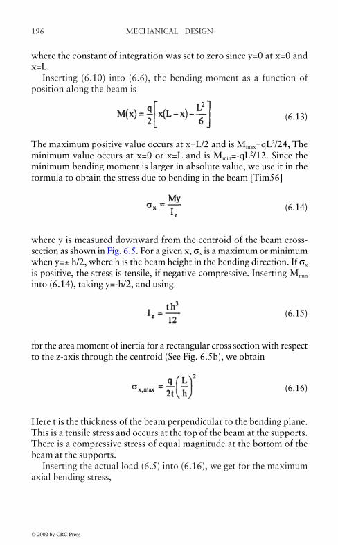
MECHANICAL DESIGN196
where the constant of integration was set to zero since y=0 at x=0 andx=L.
Inserting (6.10) into (6.6), the bending moment as a function ofposition along the beam is
(6.13)
The maximum positive value occurs at x=L/2 and is Mmax=qL2/24, Theminimum value occurs at x=0 or x=L and is Mmin=-qL2/12. Since theminimum bending moment is larger in absolute value, we use it in theformula to obtain the stress due to bending in the beam [Tim56]
(6.14)
where y is measured downward from the centroid of the beam cross-section as shown in Fig. 6.5. For a given x, σx is a maximum or minimumwhen y=± h/2, where h is the beam height in the bending direction. If σx
is positive, the stress is tensile, if negative compressive. Inserting Mmin
into (6.14), taking y=-h/2, and using
(6.15)
for the area moment of inertia for a rectangular cross section with respectto the z-axis through the centroid (See Fig. 6.5b), we obtain
(6.16)
Here t is the thickness of the beam perpendicular to the bending plane.This is a tensile stress and occurs at the top of the beam at the supports.There is a compressive stress of equal magnitude at the bottom of thebeam at the supports.
Inserting the actual load (6.5) into (6.16), we get for the maximumaxial bending stress,
© 2002 by CRC Press

197MECHANICAL DESIGN
(6.17)
The span length, L, can be determined from the number of key spacers,their width, and the mean circumference,
(6.18)
The strand height h and thickness t apply to a single strand, whether aspart of a cable having many strands or as a single strand in a magnetwire. If the cable is bonded, the maximum axial bending stress in (6.17)is divided by 3. This is simply an empirical correction to take intoaccount the greater rigidity of bonded cable.
6.3.3 Tilting Strength
The axial compressive force which is applied to the key spacers cancause the individual strands of the conductors which are pressed betweenthe key spacers to tilt if the force is large enough. Fig. 6.6 shows anidealized geometry’ of this situation. Depicted is an individual strandwhich has the form of a closed ring acted on by a uniform axialcompressive pressure, Pc. We assume initially that the strand has roundedends which do not dig into the adjacent key spacers to prevent or opposethe tilting shown, (There could be several layers of strands in the axialdirection separated by paper, which plays the same role as the keyspacers in the figure.)
Analyzing a small section in the azimuthal direction of length ∆,the applied pressure exerts a torque, τc, given by
τc=Pc(t∆)hsinθ (6.19)
where t is the radial thickness of the strand and where t ∆ is the area onwhich the pressure Pc acts. The axial height of the strand is h and θ is thetilting angle from the vertical which is assumed to be small. The tiltingcauses the material of the ring to stretch above its axial center and tocompress below it. This produces stresses in the ring which in turn producea torque which opposes the torque calculated above. To calculate thisopposing torque, let y measure the distance above the axial center of the
© 2002 by CRC Press

MECHANICAL DESIGN198
strand as shown in Fig. 6.6b. The increase in radius at distance y abovethe center line is y tanθ. Therefore the strain at position y is
(6.20)
where ε is an azimuthal strain. This produces an azimuthal tensile stress(hoop stress) given by
(6.21)
where E is Young’s modulus for the conductor material. This hoop stressresults in an inward force, Fr, on the section of strand given by
(6.22)
In (6.22) t ∆y is the area at height y over which the stress σ acts ∆ϕ andthe angle subtended by the azimuthal section of strand of length ∆.Also ∆=R∆ϕ has been used.
© 2002 by CRC Press
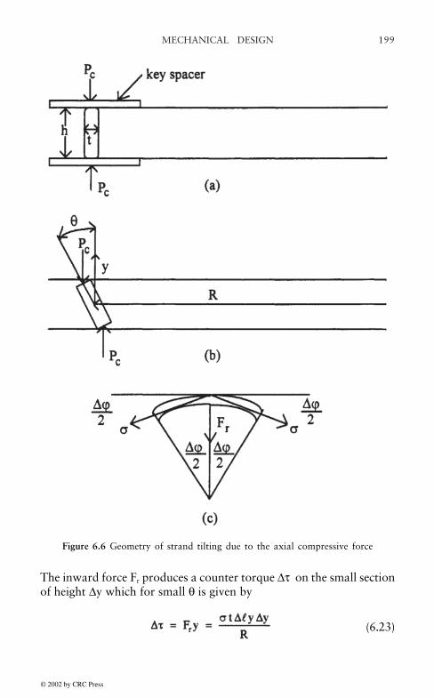
199MECHANICAL DESIGN
The inward force Fr produces a counter torque ∆τ on the small sectionof height ∆y which for small θ is given by
(6.23)
Figure 6.6 Geometry of strand tilting due to the axial compressive force
© 2002 by CRC Press
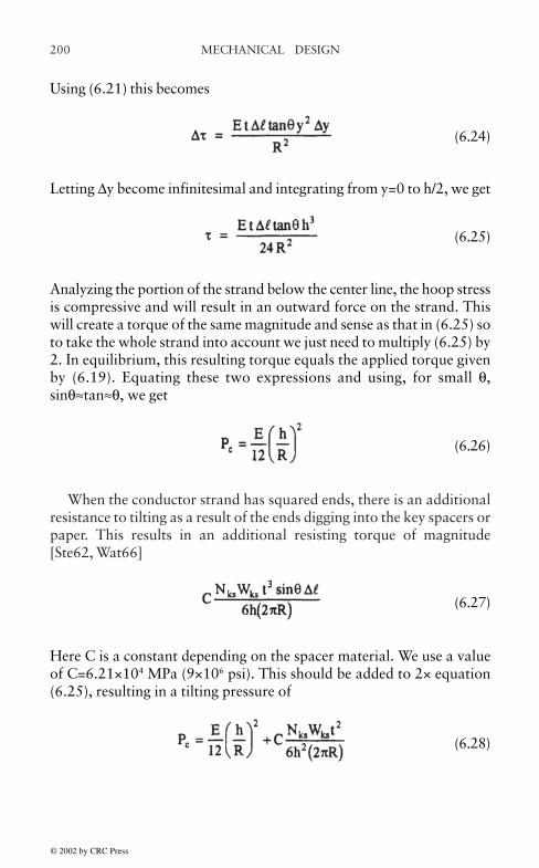
MECHANICAL DESIGN200
Using (6.21) this becomes
(6.24)
Letting ∆y become infinitesimal and integrating from y=0 to h/2, we get
(6.25)
Analyzing the portion of the strand below the center line, the hoop stressis compressive and will result in an outward force on the strand. Thiswill create a torque of the same magnitude and sense as that in (6.25) soto take the whole strand into account we just need to multiply (6.25) by2. In equilibrium, this resulting torque equals the applied torque givenby (6.19). Equating these two expressions and using, for small θ,sinθ≈tan≈θ, we get
(6.26)
When the conductor strand has squared ends, there is an additionalresistance to tilting as a result of the ends digging into the key spacers orpaper. This results in an additional resisting torque of magnitude[Ste62, Wat66]
(6.27)
Here C is a constant depending on the spacer material. We use a valueof C=6.21×10⁴ MPa (9×10⁶ psi). This should be added to 2× equation(6.25), resulting in a tilting pressure of
(6.28)
© 2002 by CRC Press

201MECHANICAL DESIGN
If the strand has rounded corners of radius Rc, then t in the above formulais reduced by 2Rc so only its flat portion is considered. The resultingcritical axial pressure is therefore
(6.29)
For comparison with the applied maximum axial compressive force,we multiply (6.29) by the radial surface area of the strands in onehorizontal layer, Alayer. This is
(6.30)
where Nd is the number of turns in a disk or section and the othersymbols have been defined previously. Note that as a result of the strandpositioning in a cable as shown in Fig. 6.4b, the expression (Nst-1)/2gives the number of strands radially that are part of the double layer.For magnet wire, the expression in parentheses is taken as 1. Thus thecritical axial force is
Fcr=PcAlayer (6.31)
This applies to unbonded cable. For bonded cable, we take Fcr=since itis assumed in this case that tilting cannot occur. We compare (6.31)with the maximum applied axial compressive force, Fc, by taking theratio, Fcr/Fc. This ratio must be >1 for a viable design, i.e. Fc must be<Fcr.
In the above derivation, the compressive force was assumed to beapplied uniformly around the strand ring, whereas in reality it is onlyapplied to the portions of the ring in contact with the key spacers. Sincethe portions outside the key spacers see no applied pressure, theuniformly applied pressure represents an averaging process over theentire ring and is a reasonable approximation,
6.3.4 Stress in Tie Bars
The tie bars or tieplates are used to join the upper and lower clampingstructures which keep the coils under compression. These are generally
© 2002 by CRC Press

MECHANICAL DESIGN202
long rectangular bars of steel which are placed along the sides of thecore legs. They are under mild tension during normal transformeroperation. During short circuit, the tensile stresses can increaseconsiderably. Also when the transformer is lifted, the tie bars supportthe entire weight of the coils and core.
The short circuit stress in the tie bars is due to the total end thrustproduced by all the coils. This is the sum of the total upward ordownward forces acting on the coils and is an output of the forceprogram. Since this output refers to a single leg, the tie bars affected bythis force should only be those associated with a single leg. In the caseof a 3 phase fault, all the tie bars are affected equally. However, in thecase of a single line to ground fault where the forces are much higher onone leg than the other two, the tie bars associated with the leg havingthe greater force will probably experience the greatest stress. Thereforein this worst case scenario, we are assuming that the legs actindependently at least for the short duration of the fault.
The total end thrust is the result of a static force calculation. Becauseof possible dynamic effects associated with the sudden application of aforce to an elastic system, the end thrust could be considerably higherfor a short period after the force application. To see what the dynamicforce enhancement might be, we analyze an elastic bar subject to asuddenly applied force as illustrated in Fig. 6.7. Let x measure thechange in length produced by the force, relative to the unstressed bar oflength L. A bar under stress stores elastic energy, U, given by [Tim56]
(6.32)
where E is Young’s modulus for the bar material and A is the cross-sectional area of the bar. The applied force causes the bar material tomove so that it acquires a kinetic energy. Since each portion of the barmoves with a different velocity—the bar is fixed at one end and moveswith maximum velocity at the other end—it is necessary to integrate thekinetic energy of each segment along the bar to get the total. In Fig.6.7a, a bar segment a distance y from the fixed end of thickness dy isisolated. The parameter u measures the displacement of this bar segmentand its velocity is therefore du/dt. But the strain ε is uniform along thebar so we have ε=u/y=x/L. Therefore u=xy/L and du/dt=(y/L) dx/dt. Thesegment’s kinetic energy is
© 2002 by CRC Press
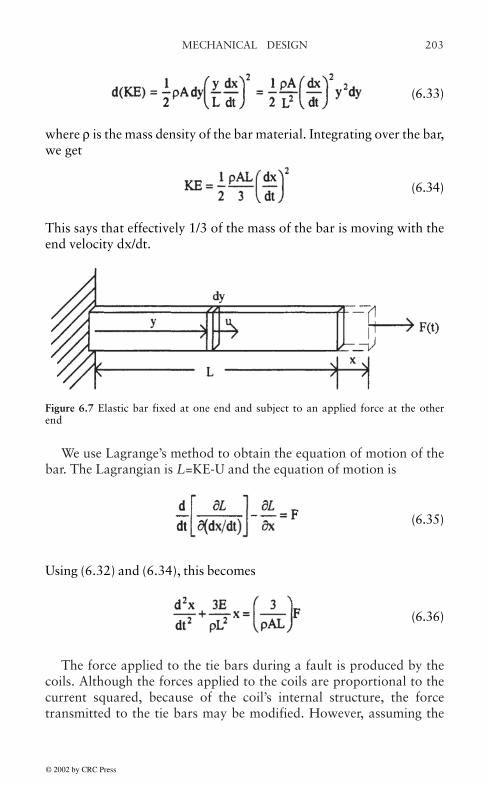
203MECHANICAL DESIGN
We use Lagrange’s method to obtain the equation of motion of thebar. The Lagrangian is L=KE-U and the equation of motion is
(6.35)
Using (6.32) and (6.34), this becomes
(6.36)
The force applied to the tie bars during a fault is produced by thecoils. Although the forces applied to the coils are proportional to thecurrent squared, because of the coil’s internal structure, the forcetransmitted to the tie bars may be modified. However, assuming the
(6.33)
where ρ is the mass density of the bar material. Integrating over the bar,we get
(6.34)
This says that effectively 1/3 of the mass of the bar is moving with theend velocity dx/dt.
Figure 6.7 Elastic bar fixed at one end and subject to an applied force at the otherend
© 2002 by CRC Press
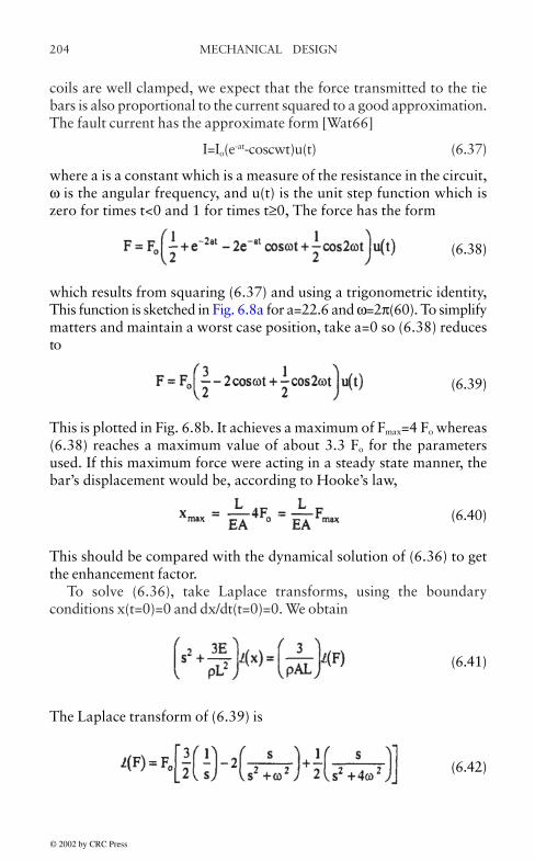
MECHANICAL DESIGN204
coils are well clamped, we expect that the force transmitted to the tiebars is also proportional to the current squared to a good approximation.The fault current has the approximate form [Wat66]
I=Io(e-at-coscwt)u(t) (6.37)
where a is a constant which is a measure of the resistance in the circuit,ω is the angular frequency, and u(t) is the unit step function which iszero for times t<0 and 1 for times t≥0, The force has the form
(6.38)
which results from squaring (6.37) and using a trigonometric identity,This function is sketched in Fig. 6.8a for a=22.6 and ω=2π(60). To simplifymatters and maintain a worst case position, take a=0 so (6.38) reducesto
(6.39)
This is plotted in Fig. 6.8b. It achieves a maximum of Fmax=4 Fo whereas(6.38) reaches a maximum value of about 3.3 Fo for the parametersused. If this maximum force were acting in a steady state manner, thebar’s displacement would be, according to Hooke’s law,
(6.40)
This should be compared with the dynamical solution of (6.36) to getthe enhancement factor.
To solve (6.36), take Laplace transforms, using the boundaryconditions x(t=0)=0 and dx/dt(t=0)=0. We obtain
(6.41)
The Laplace transform of (6.39) is
(6.42)
© 2002 by CRC Press
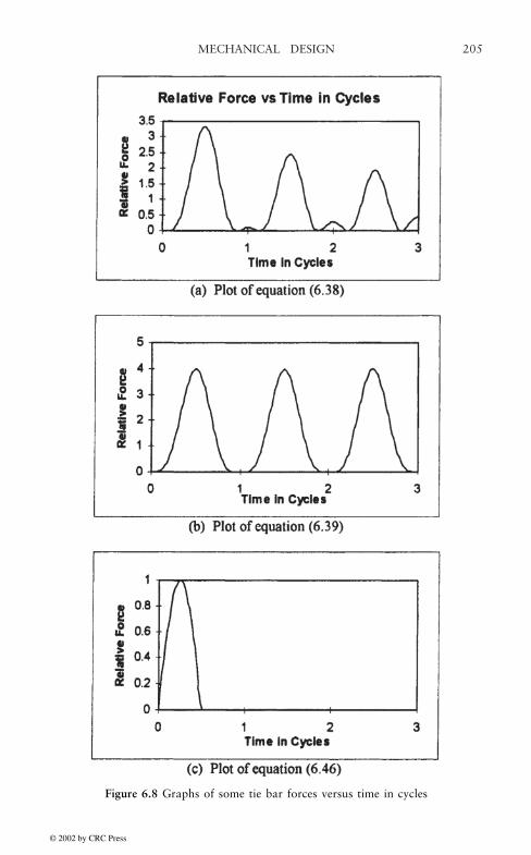
205MECHANICAL DESIGN
Figure 6.8 Graphs of some tie bar forces versus time in cycles
© 2002 by CRC Press

MECHANICAL DESIGN206
Substituting into (6.41), we obtain for the Laplace transform of x
(6.43)
where b2=3E/ρL2. Using some algebra to rewrite (6.43) and taking inversetransforms, we obtain
where the quantity in curly brackets is the enhancement factor.We need to compare the natural angular frequency b with the
applied angular frequencies ω=2πf=377 Rads/sec, assuming f=60 Hz,and 2ω=754 Rads/sec to see whether a resonance problem might occur.For steel bars, E=2.07×10⁵ MPa (30×106 psi), ρg=7.68×10⁴ N/m3 (0.283lb/in3), where g is the acceleration of gravity=9.8 m/sec2 (386 in/sec2).Thus, we obtain for b,
(6.45)
For a 2.54m (100 in) long tie bar which is typical, this gives b=3504Rads/sec. Since this is much larger than ω or 2ω, we are far fromresonance. Thus (ω/b)2 can be ignored relative to 1 in (6.44) and itsimplifies to x(t)=(L/EA) F with F given by (6.39). Hence xmax is thesame as in the steady-state case and the enhancement factor is 1. Thus,unless the applied or twice the applied frequency is close to the tie bar’snatural frequency, there is no dynamic enhancement. By numericallychecking over a large grid of times and frequencies, a maximumenhancement of about 1.66 is produced if the time does not exceed oneperiod (ωt<2π). However as time increases, the maximum enhancementfactor gradually increases when we are near resonance. This is to beexpected since there is no damping in the problem and no cut-off of theforce.
(6.44)
© 2002 by CRC Press

207MECHANICAL DESIGN
Another perhaps more realistic approximation to the applied force isprovided by a half wave pulse given by
(6.46)
where u(t) is a unit step at t=0 and u(t”π/ω) is a unit step at t=π/ω. Thisis illustrated in Fig. 6.8c. The Laplace transform of (6.46) is
(6.47)
Substituting into (6.41), we obtain for the Laplace transform of x,
(6.48)
Taking the inverse transform, we get
where the quantity in curly brackets is the enhancement factor. For b>>ω, we get the static response x=(L/EA) F, with F given by (6.46), i.e. thebar extension is just proportional to the force with no enhancement. Bynumerically checking over a large grid of times and frequencies, themaximum enhancement factor obtained was 1.77.
In practice, we use a force of 1.8 times the end thrust provided it islarger than 0.8 times the maximum compressive force over all thewindings. Otherwise we use 0.8 times the maximum compressive forceover all the windings. However, since the tie bars must support the
(6.49)
© 2002 by CRC Press

MECHANICAL DESIGN208
weight of the core and coils during lifting, we check the stress in the tiebars produced by lifting. During lifting, we only assume the tie barsassociated with the outer legs are stressed since this is where the liftinghooks are positioned. Both the short circuit dynamic stresses and thelifting stresses must be below a maximum allowable stress in the tie barmaterial. We take this maximum allowable stress to be 620 MPa(90,000 psi) if a low carbon steel is used and 414 MPa (60,000 psi) if astainless steel is used for the tie bar material,
6.3.5 Stress in the Pressure Rings
The pressure ring receives the total end thrust of the windings. In ourdesigns, it is made of pressboard of about 3.8 to 6.35 cm (1.5 to 2.5 in)thickness. The ring covers the radial build of the windings with a littleoverhang. During a fault, it must support the full dynamic end thrust ofthe windings, which according to the last section is 1.8 times the totalend thrust or 0.8 times the maximum compressive force in all the windingswhichever is larger.
The end thrust or force is distributed over the end ring, producing aneffective pressure of
(6.50)
where we use ring to label the end force, Fring, and ring area, Aring. Thisarea is given by
(6.51)
in terms of the outer and inner ring diameters. The ring is supported onradial blocks with space between for the leads. This produces anunsupported span of a certain length Lu. To a good approximation, theproblem is similar to that discussed previously for the axial bending ofa strand of wire. Thus we can use formula (6.16) for the maximumstress in the end ring, with L=Lu, t=(1/2)(Dring,out–Dring,in) the radial buildof the ring, h=hring the ring’s thickness, and q=Pring t the force/unit lengthalong the unsupported span. We obtain
(6.52)
© 2002 by CRC Press

209MECHANICAL DESIGN
For our pressboard rings, the maximum bending stress permissible isσbend=103 MPa (15,000 psi), Substituting this value for σx,max and solvingfor Fring corresponding to this limiting stress, we find
(6.53)
This is the maximum end force the pressure ring can sustain. It must begreater than the applied maximum end force.
6.3.6 Hoop Stress
The maximum radial pressure acting on the winding as obtained fromthe force program creates a hoop stress in the winding conductor. Thehoop stress is tensile or compressive, depending on whether the pressureacts radially outwards or inwards respectively. In Fig. 6.9, we treat thewinding as an ideal cylinder or ring subjected to a radially inwardpressure, Pr. Let Rm be the mean radius of the cylinder and H its axialheight. In part (b) of the figure, we show 2 compressive reaction forcesF in the winding, sustaining the force applied to half the cylinder. The xdirected force produced by the pressure Pr cancels out by symmetry andthe net y directed force acting downward is given by
(6.54)
This is balanced by a force of 2F acting upward so we get F=PrHRm.Dividing by the cross sectional area A of the material sustaining theforce, we get the compressive stress in the material
(6.55)
For A=HB, where B is the radial build of the cylinder, we get
(6.56)
© 2002 by CRC Press

MECHANICAL DESIGN210
This last formula assumes the cylinder is made of a homogeneousmaterial. If the cylinder is made of conductors and insulating materials,the conductors primarily support the forces. In this case A should equalthe cross-sectional area of all the conductors in the winding, A=AtNt,where At is the cross-sectional area of a turn and Nt is the total numberof turns in the winding. If the winding is center fed, i.e. consists of twoparallel windings on the same leg, and Nt refers to the total turns/leg ortwice the number of electrical turns, then At should be 1/2 the turn area.Substituting into (6.55) and using Dm=2Rm, we obtain
(6.57)
Figure 6.9 Geometry for determining the hoop stress in a cylinder acted on by aradially inward pressure
© 2002 by CRC Press

211MECHANICAL DESIGN
for the hoop stress. This is compressive for Pr acting inward and tensilefor Pr acting outward. In either case, this stress should not exceed theproof stress of the winding material.
When the radial pressure acts inwards, the winding is apt to bucklebefore the proof stress is exceeded. This inward radial buckling is acomplex process to analyze. We will present an idealized analysis later.Based on limited experimental results, it has been suggested that thiscompressive hoop stress not exceed some fraction of the proof stress, thefraction varying from 0.4 to 0.7 depending on the type of cable usedand whether it is bonded.
6.3.7 Radial Bending Stress
Windings have inner radial supports such as sticks made of pressboardwhich are spaced uniformly along their circumference and extend theheight of the winding. When an inward radial pressure acts on thewinding, the sections of the winding between supports act like a curvedbeam subjected to a uniform loading. A similar situation occurs in thecase of a rotating flywheel with radial spokes. In the flywheel case, theloading (centrifugal force) acts outwards but otherwise the analysis issimilar. The flywheel example is analyzed in Timoshenko [Tim56] whichwe follow here with minor changes.
We need to make use of Castigliano’s theorem. This states that if thematerial of a system follows Hooke’s law, i.e. remains within the elasticlimit, and if the displacements are small, then the partial derivative ofthe strain energy with respect to any force equals the displacementcorresponding to the force. Here force and displacement have ageneralized meaning, i.e. they could refer to torques or moments andangular displacements as well as their usual meanings of force andlength displacements. Also the strain energy must be expressed as aquadratic function of the forces. For example, the strain energyassociated with tensile or compressive forces N in a beam of length L is
(6.58)
where N, A, and E , can be functions of position along the beam , x.The strain energy associated with a bending moment M in a beam oflength L is
© 2002 by CRC Press

MECHANICAL DESIGN212
(6.59)
where M , I, and E can be functions of position, x Here I is the areamoment of inertia.
In Fig. 6.10a, we show a portion of the winding with the inner radialsupports spaced an angle 2α apart. There is a normal force X actingradially outwards at the supports which counters the inward pressurewhich has been converted to a force/unit length q acting on the coilsection. The coil section is assumed to form a closed ring of radial buildh, axial height t, and mean radius R.
In Fig. 6.10b, we further isolate a portion of the ring which extendsbetween adjacent mid-sections between the supports. The reason fordoing this is that there is no radially directed (shearing) force acting onthese mid cross-sections. This is because by symmetry, the distributedload between the mid-sections must balance the outward force at theincluded support. Thus the only reactions at the midsections are anazimuthally directed force No and a couple Mo which need to be found.
Figure 6.10 Geometry for determining the radial bending stresses
© 2002 by CRC Press

213MECHANICAL DESIGN
Balancing the vertical forces, we have
(6.60)
Performing the integral and solving for No, we obtain
(6.61)
At any cross-section as shown in Fig. 6.10c, measuring angles fromthe mid-section position with the variable ϕ, we can obtain the normalforce, N, from the static equilibrium requirement
(6.62)
Integrating and substituting for No from (6.61), we get
(6.63)
Similarly, using Fig. 6.10d,e, we can obtain the bending moment atthe cross-section an angle ϕ from the mid-section by balancing themoments
(6.64)
Performing the integration and substituting for No from (6.61), we obtain
(6.65)
Equations (6.63) and (6.65) express the normal force and bendingmoments as functions of position along the beam (arc in this case).These can be used in the energy expressions (6.58) and (6.59).
© 2002 by CRC Press
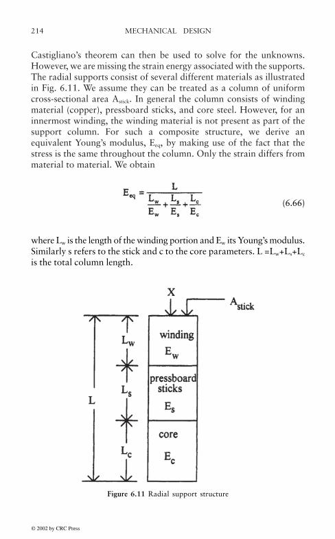
MECHANICAL DESIGN214
Castigliano’s theorem can then be used to solve for the unknowns.However, we are missing the strain energy associated with the supports.The radial supports consist of several different materials as illustratedin Fig. 6.11. We assume they can be treated as a column of uniformcross-sectional area Astick. In general the column consists of windingmaterial (copper), pressboard sticks, and core steel. However, for aninnermost winding, the winding material is not present as part of thesupport column. For such a composite structure, we derive anequivalent Young’s modulus, Eeq, by making use of the fact that thestress is the same throughout the column. Only the strain differs frommaterial to material. We obtain
(6.66)
where Lw is the length of the winding portion and Ew its Young’s modulus.Similarly s refers to the stick and c to the core parameters. L =Lw+Ls+Lc
is the total column length.
Figure 6.11 Radial support structure
© 2002 by CRC Press
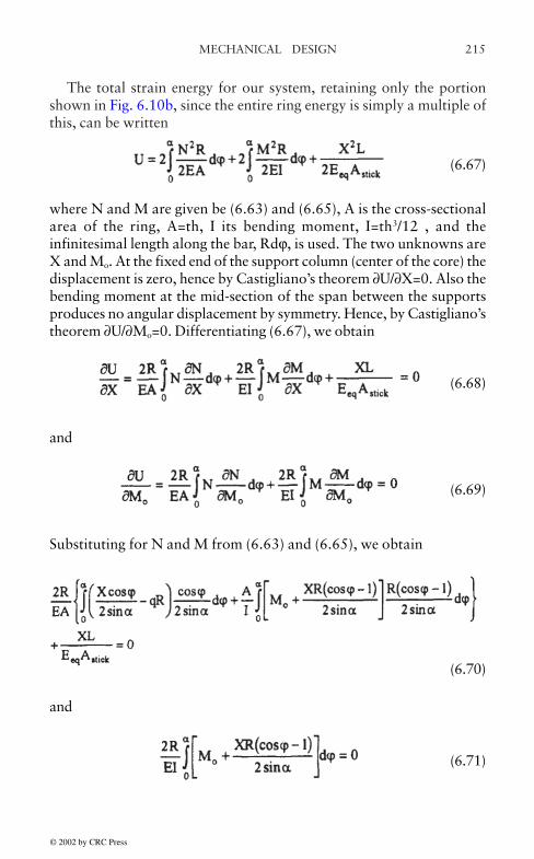
215MECHANICAL DESIGN
The total strain energy for our system, retaining only the portionshown in Fig. 6.10b, since the entire ring energy is simply a multiple ofthis, can be written
(6.67)
where N and M are given be (6.63) and (6.65), A is the cross-sectionalarea of the ring, A=th, I its bending moment, I=th3/12 , and theinfinitesimal length along the bar, Rdϕ, is used. The two unknowns areX and Mo. At the fixed end of the support column (center of the core) thedisplacement is zero, hence by Castigliano’s theorem ∂U/∂X=0. Also thebending moment at the mid-section of the span between the supportsproduces no angular displacement by symmetry. Hence, by Castigliano’stheorem ∂U/∂Mo=0. Differentiating (6.67), we obtain
(6.68)
and
(6.69)
Substituting for N and M from (6.63) and (6.65), we obtain
and
(6.71)
(6.70)
© 2002 by CRC Press

MECHANICAL DESIGN216
Integrating the above expressions, we obtain
(6.72)
and
(6.73)
where we have used the fact that L=R. Substituting into (6.63) and (6.65)and defining
(6.74)
we obtain for N and M
(6.75)
(6.76)
We also have
© 2002 by CRC Press

217MECHANICAL DESIGN
(6.77)
where h is the radial build of the ring. N gives rise to a normal stress
and M gives rise to a bending stress which varies over the cross-section,achieving a maximum tensile or compressive value of (see formula (6.14))
We have factored out the term qR/A since this can be shown to be thehoop stress in the ring. (In formula (6.55), PH corresponds to q and Rmto R in our development here.) Thus σhoop will be substituted in thefollowing formulas for qR/A, where σhoop is given by (6.57).
We now need to add σN and σM in such a way as to produce the worstcase stress in the ring. The quantity
(6.80)
occurs in both stress formulas. We have tabulated f1(α), f2(α), and sintimes these in Table 6.1 for a range of α values.
(6.78)
(6.79)
© 2002 by CRC Press

MECHANICAL DESIGN218
It can be see that for any choice of the other parameters (6.80) ispositive. In (6.79), the magnitude of σM for fixed is determined by theterm (cosϕ sinα/α), where ϕ can range from 0 to α. This achieves amaximum in absolute value at ϕ=α. The stress can have either signdepending on whether it is on the inner radial or outer radial surface ofthe ring. In (6.78), the magnitude of σN achieves a maximum at ϕ=α forvirtually any choice of the other parameters. It has a negative signconsistent with the compressive nature of the applied force. Thus σN
and σM should be added with each having a negative sign at ϕ=α to getthe maximum stress. We obtain
Table 6.1 Tabulated values for f1(α) and f2(α) and sin times these quantities
This stress is negative although it is usually quoted as a positive number.It occurs at the support.
(6.81)
© 2002 by CRC Press
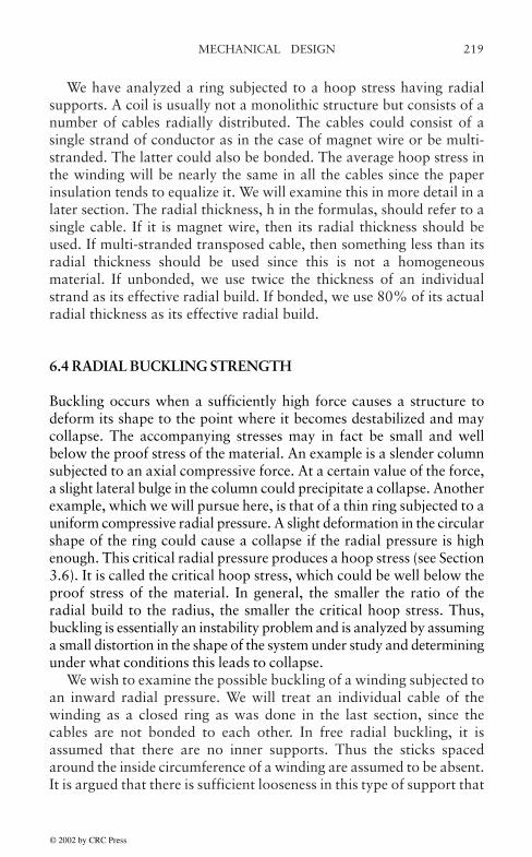
219MECHANICAL DESIGN
We have analyzed a ring subjected to a hoop stress having radialsupports. A coil is usually not a monolithic structure but consists of anumber of cables radially distributed. The cables could consist of asingle strand of conductor as in the case of magnet wire or be multi-stranded. The latter could also be bonded. The average hoop stress inthe winding will be nearly the same in all the cables since the paperinsulation tends to equalize it. We will examine this in more detail in alater section. The radial thickness, h in the formulas, should refer to asingle cable. If it is magnet wire, then its radial thickness should beused. If multi-stranded transposed cable, then something less than itsradial thickness should be used since this is not a homogeneousmaterial. If unbonded, we use twice the thickness of an individualstrand as its effective radial build. If bonded, we use 80% of its actualradial thickness as its effective radial build.
6.4 RADIAL BUCKLING STRENGTH
Buckling occurs when a sufficiently high force causes a structure todeform its shape to the point where it becomes destabilized and maycollapse. The accompanying stresses may in fact be small and wellbelow the proof stress of the material. An example is a slender columnsubjected to an axial compressive force. At a certain value of the force,a slight lateral bulge in the column could precipitate a collapse. Anotherexample, which we will pursue here, is that of a thin ring subjected to auniform compressive radial pressure. A slight deformation in the circularshape of the ring could cause a collapse if the radial pressure is highenough. This critical radial pressure produces a hoop stress (see Section3.6). It is called the critical hoop stress, which could be well below theproof stress of the material. In general, the smaller the ratio of theradial build to the radius, the smaller the critical hoop stress. Thus,buckling is essentially an instability problem and is analyzed by assuminga small distortion in the shape of the system under study and determiningunder what conditions this leads to collapse.
We wish to examine the possible buckling of a winding subjected toan inward radial pressure. We will treat an individual cable of thewinding as a closed ring as was done in the last section, since thecables are not bonded to each other. In free radial buckling, it isassumed that there are no inner supports. Thus the sticks spacedaround the inside circumference of a winding are assumed to be absent.It is argued that there is sufficient looseness in this type of support that
© 2002 by CRC Press

MECHANICAL DESIGN220
the onset of buckling occurs as if these supports were absent and oncestarted, the buckling process continues towards collapse or permanentdeformation. It could also be argued that even though buckling maybegin in the absence of supports, before it progresses very far thesupports are engaged and from then on it becomes a different type ofbuckling, called forced or constrained buckling. The key to the lastargument is that even though free buckling has begun, the stresses inthe material are quite low, resulting in no permanent deformation andthe process is halted before collapse can occur.
We will analyze free buckling of a circular ring in some detail andquote the results for forced buckling. The lowest order shape distortionaway from a circle is taken to be an ellipse [Tim56]. This is shown inFig. 6.12 along with the parameters used to describe the system. With umeasuring the displacement radially inward from the circular shape,the differential equation for the deflection of a thin bar (ring) withcircular center line of radius R is [Tim56]
(6.82)
where s is the length along the bar. Since s=Rdϕ where the angle ϕ isshown in Fig. 6.12, ds2=R2dϕ2, and (6.82) can be written
(6.83)
Here M is the bending moment along the ring, E is Young’s modulus,and I the area moment of inertia.
© 2002 by CRC Press

221MECHANICAL DESIGN
By symmetry, we need only consider one quadrant of the ring and wehave chosen the upper right quadrant. We wish to determine the bendingmoment at a cross-section B at an angle ϕ from the x axis as shown inFig. 6.12. Consider the equilibrium of the section of the ring from A toB. At the cross-section A there is an unknown normal force No and anunknown bending moment Mo acting. From symmetry, no shearing forceacts at A. The bending moment at B has a contribution from Mo, fromNo, and from the distributed force/unit length q acting on the segmentfrom A to B.
The moment at B due to Mo is just Mo and the moment at B due to No
is
Figure 6.12 Buckling of a circular ring. The distorted elliptical shape and itsparametrization are shown.
© 2002 by CRC Press
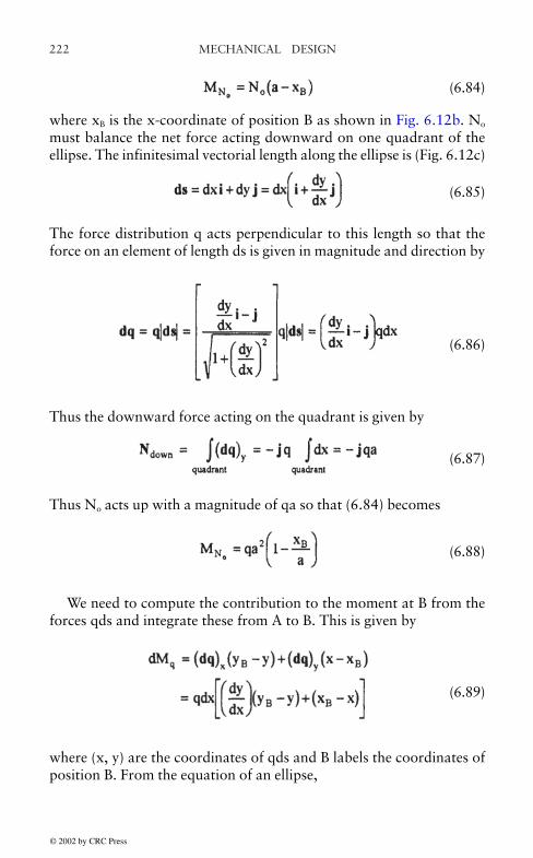
MECHANICAL DESIGN222
(6.84)
where xB is the x-coordinate of position B as shown in Fig. 6.12b. No
must balance the net force acting downward on one quadrant of theellipse. The infinitesimal vectorial length along the ellipse is (Fig. 6.12c)
(6.85)
The force distribution q acts perpendicular to this length so that theforce on an element of length ds is given in magnitude and direction by
(6.86)
Thus the downward force acting on the quadrant is given by
(6.87)
Thus No acts up with a magnitude of qa so that (6.84) becomes
(6.88)
We need to compute the contribution to the moment at B from theforces qds and integrate these from A to B. This is given by
(6.89)
where (x, y) are the coordinates of qds and B labels the coordinates ofposition B. From the equation of an ellipse,
© 2002 by CRC Press

223MECHANICAL DESIGN
(6.90)
we obtain
(6.91)
Substituting into (6.89), we obtain
(6.92)
Integrating from x=xB to x=a, we get
Adding the contributions to M at B, Mo, (6.88) and (6.93), we get
(6.94)
In terms of uo in Fig. 6.12, we have for uo small compared with R
(6.95)
Therefore
b2-a2=4Ruo (6.96)
(6.93)
© 2002 by CRC Press

MECHANICAL DESIGN224
The equation of an ellipse in polar coordinates is
(6.97)
where (6.96) has been used to obtain the second approximate equality.For small deviations from a circular shape (uo<<R), (6.97) becomesapproximately
(6.98)
Using (6.95), this becomes
(6.99)
Retaining only terms linear in uo, we get
(6.100)
Letting xB=a cos for small uo, (6.100) becomes
(6.101)
From Fig. 6.12,
(6.102)
© 2002 by CRC Press

225MECHANICAL DESIGN
Therefore,
(6.103)
Substituting (6.96) and (6.103) into (6.94), we obtain
M=Mo-qR(uo-u) (6.104)
Substituting (6.104) into (6.83), the differential equation becomes
(6.105)
The general solution to this equation is
(6.106)
where A and B are constants to be determined by the boundary conditionsand
(6.107)
We can see from the shape of the ellipse that a choice of boundaryconditions for (6.105) is
(6.108)
These yield
(6.109)
The second equation above can be satisfied if p=2n for n=1, 2, 3, …. Forn=1, (6.107) becomes
© 2002 by CRC Press

MECHANICAL DESIGN226
(6.110)
which can be re-expressed as
(6.111)
This is the critical buckling force/unit length since it is associated withan angular dependence of u which corresponds to an elliptical shape.
We can find the critical hoop stress associated with q in (6.111) bymeans of the expression σhoop=qR/A developed earlier (see the discussionfollowing formula (6.79)). Thus
(6.112)
For a ring with a radial build of h and an axial height of t (see Fig.6.10), we have A=th and I=th3/12 so that (6.112) becomes
(6.113)
Thus the critical hoop stress depends geometrically only on the ratio ofthe radial build to the radius of the ring.
Since buckling occurs after the stress has built up in the ring to thecritical value and increases incrementally beyond it, the appropriatemodulus to use in (6.113) is the tangential modulus since this isassociated with incremental changes. This argument for using thetangential modulus is based on an analogous argument for the bucklingof slender columns together with supporting experimental evidencegiven in Ref. [Tim56]. We will assume it applies to thin rings as well.
The tangential modulus can be obtained graphically from the stress-strain curve for the material as illustrated in Fig. 6.13a. However, forcopper which is the material of interest here, the stress-strain curve canbe parametrized for copper of different hardnesses according to [Tho79]by
© 2002 by CRC Press

227MECHANICAL DESIGN
(6.114)
where k=3/7, m=11.6, and Eo=1.10×10⁵ MPa (16×106 psi). σo dependson the copper hardness. The tangential modulus obtained from this is
(6.115)
where γ=k(m+1)=5.4. Substituting Et from (6.115) for E in (6.113), weobtain a formula for self-consistently determining the critical stress,
(6.116)
This can be solved by Newton-Raphson iteration,
Figure 6.13 Stress-strain curve and derived quantities
© 2002 by CRC Press

MECHANICAL DESIGN228
The parameter σo is generally not provided by the wire or cablesupplier. It could be obtained by fitting a supplied stress-strain curve.Alternatively and more simply, it can be obtained from the proof stressof the material which is generally provided or specified. As one movesalong a stress-strain curve and then removes the stress, the materialdoes not move back towards zero stress along the same curve itfollowed when the stress increased but rather it follows a straight lineparallel to the initial slope of the stress-strain curve as illustrated in Fig.6.13b. This leaves a residual strain in the material, labeled εp in thefigure, corresponding to the stress σp which was the highest stressachieved before it was removed. For εp=0.002 (0.2%), σp is called theproof stress. (Some people use εp=0.001 in this definition.)
Thus the proof stress is determined from the intersection of the recoilline
σ=Eo(ε-εp) (6.117)
with the stress-strain curve given by (6.114). Solving (6.114) and (6.117)simultaneously, we find
(6.118)
This permits us to find σo from a given proof stress σp corresponding tothe appropriate εp.
When the supports (sticks) are engaged in the buckling process, wehave forced or constrained buckling. Since there is some looseness inthe support due to building tolerances, it can be regarded as a hingedtype of attachment for caiculational purposes. In this case, the lowestorder buckling mode is shown in Fig. 6.14. The corresponding criticalforce/unit length, qcrit, is given by [Tim56]
(6.119)
where β is the angle between the supports. This corresponds to a criticalhoop stress of
© 2002 by CRC Press
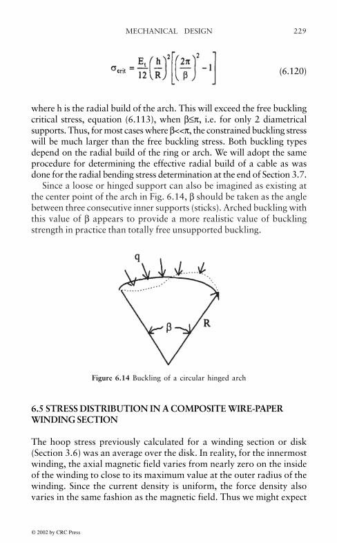
229MECHANICAL DESIGN
(6.120)
where h is the radial build of the arch. This will exceed the free bucklingcritical stress, equation (6.113), when β≤π, i.e. for only 2 diametricalsupports. Thus, for most cases where β<<π, the constrained buckling stresswill be much larger than the free buckling stress. Both buckling typesdepend on the radial build of the ring or arch. We will adopt the sameprocedure for determining the effective radial build of a cable as wasdone for the radial bending stress determination at the end of Section 3.7.
Since a loose or hinged support can also be imagined as existing atthe center point of the arch in Fig. 6.14, β should be taken as the anglebetween three consecutive inner supports (sticks). Arched buckling withthis value of β appears to provide a more realistic value of bucklingstrength in practice than totally free unsupported buckling.
6.5 STRESS DISTRIBUTION IN A COMPOSITE WIRE-PAPERWINDING SECTION
The hoop stress previously calculated for a winding section or disk(Section 3.6) was an average over the disk. In reality, for the innermostwinding, the axial magnetic field varies from nearly zero on the insideof the winding to close to its maximum value at the outer radius of thewinding. Since the current density is uniform, the force density alsovaries in the same fashion as the magnetic field. Thus we might expect
Figure 6.14 Buckling of a circular hinged arch
© 2002 by CRC Press

MECHANICAL DESIGN230
higher hoop stresses in the outermost turns as compared with the innerturns. However, because of the layered structure with paper insulationbetween turns, the stresses tend to be shared more equally by all theturns. This effect will be examined here in order to determine the extentof the stress non-uniformity so that, if necessary, corrective action canbe taken.
We analyze an ideal ring geometry as shown in Fig. 6.15. In thefigure, rci denotes the inner radius of the ith conductor layer and rpi theinner radius of the ith paper layer, where i=1,…, n for the conductorsand i=1,…, n–1 for the paper layers. Because of the assumed closecontact, the outer radius of the ith conductor layer equals the innerradius of the ith paper layer and the outer radius of the ith paper layerequals the inner radius of the i+1th conductor layer. We do not need toinclude the innermost or outermost paper layers since they areessentially stress free.
We will assume that the radial force density varies linearly from theinnermost to outermost conductor layers. Thus
Figure 6.15 Conductor-paper layered ring winding section, ci refers to conductor iand pi to paper layer i.
(6.121)
© 2002 by CRC Press

231MECHANICAL DESIGN
where fo is the maximum force density at the outermost conductor. Wewish to express this in terms of the average force density, fave. We have
(6.122)
Solving for fo and substituting into (6.121), we get
(6.123)
It is even more convenient to relate fci to the average hoop stress in thewinding resulting from these radial forces. We related this stress to theradial pressure in equation (6.56). But the average force density is justthe average radial pressure divided by the winding radial build, Thereforewe find, from (6.56)
(6.124)
where Rm is the mean radius of the winding. Thus (6.123) can be written
(6.125)
We assume that the winding section can be analyzed as a 2 dimensionalstress distribution problem, i.e. stress variations in the axial directionare assumed to be small. The governing equation for this type of problemin polar coordinates when only radial forces are acting and the geometryis cylindrically symmetric is [Tim70]
(6.126)
where σr is the radial stress, σϕ the azirnuthal stress, and fr the radialforce density. The stresses are related to the strains for the 2 dimensionalplane stress case by
(6.127)
© 2002 by CRC Press

MECHANICAL DESIGN232
where E is Young’s modulus ν and is Poisson’s ratio(ν=0.25 for mostmaterials). The radial and azimuthal strains, ετ and εϕ, are related tothe radial displacement u, in the cylindrically symmetric case, by
(6.128)
Substituting (6.127) and (6.128) into (6.126), we obtain
(6.129)
with the general solution,
(6.130)
where A and B are constants to be determined by the boundaryconditions and
(6.131)
Note that for our problem, fr is negative (radially inwards) so that K ispositive. In the paper layers, K=0 since there is no force density there.Using (6.130) for u in (6.127) and (6.128), we obtain
(6.132)
The solution (6.130), (6.131), and (6.132) applies to each layer ofconductor or paper. We therefore need to introduce labels to distinguishthe layers. Let Aci, Bci apply to conductor layer i and Api, Bpi apply topaper layer i. Let ci and pi also label the displacements, u, and the
© 2002 by CRC Press

233MECHANICAL DESIGN
stresses σr, σϕ for the corresponding layer. At the conductor-paperinterface, the displacements must match,
(6.133)
There are 2(n-1) such equations. (See Fig. 6.15 for the labeling.) Alsoat the interface, the radial stresses must match,
(6.134)
There are also 2(n-1) such equations. We also have, at the innermostand outermost radii,
(6.135)
This provides 2 more equations. Thus altogether we have 4n-2 equations.There are 2 unknowns, Aci and Bci, associated with each conductor layerfor a total of 2n unknowns and 2 unknowns, Api and Bpi, associated witheach paper layer for a total of 2(n-1) unknowns since there are only n”1paper layers. Thus there are altogether 4n-2 unknowns to solve for andthis matches the number of equations. In (6.132) we must use theappropriate material constants for the conductor or paper layer, i.e.E=Ec or Ep is the conductor’s or paper’s Young’s modulus and ν=νc or νp
for the conductor’s or paper’s Poisson’s ratio. In addition K needs to belabeled according to the layer, i.e. Kci, and in the case of a paper layerKpi=0.
The resulting set of 4n-2 equations in 4n-2 unknowns is a linearsystem and can be solved by standard methods. Once the solution isobtained, (6.132) can be used to find the stresses. The σϕ can then becompared with the average hoop stress to see how much deviation thereis from a uniform distribution. We show a sample calculation in Table6.2. The average stresses are calculated for the conductor and paperand then the stresses in the layers are expressed as multipliers of this
© 2002 by CRC Press

MECHANICAL DESIGN234
average stress. These multipliers are averages for the layers since thestresses vary across a layer. The input is the geometric data and theaverage hoop stress in the conductor which is obtained from the radialpressure via (6.124). The calculated average hoop stress in theconductor does not quite agree with the input, probably because ofnumerical approximations in the averaging method. The hoop stress inthe conductors varies by about 20% from the inner to the outer layers.The other stresses are small in comparison although they showconsiderable variation across the winding. The stresses are shown aspositive, even though they are compressive and therefore negative.
Table 6.2 Sample Stress Distribution in a Composite Conductor-Paper Disk
© 2002 by CRC Press

235MECHANICAL DESIGN
6.6 ADDITIONAL MECHANICAL CONSIDERATIONS
During a short circuit, the leads or busbars are subjected to an increasedforce due to the higher fault current they carry interacting with thehigher leakage flux from the main windings and from nearby leads.These forces will depend on the detailed positioning of the leads withrespect to the main windings and with respect to each other. They willtherefore vary considerably from design to design. The leads must bebraced properly so that they do not deform or move much during afault. The leakage flux in the vicinity of the lead can be obtained froma finite element calculation. The flux produced by neighboring leadscan be determined from the Biot-Savart law. From these, the forces onthe leads can be determined and the adequacy of the bracing checked.In general, the bracing will contain sufficient margin based on pastexperience so that the above rather laborious analysis will only benecessary for unusual or novel designs.
We have neglected gravitational forces in the preceding sectionsexcept for the effect of the core and coil weight on the tie bar stressduring lifting. Gravitational forces will affect the compressive force onthe key spacers and on the downward end thrust which acts on thebottom pressure ring. Another force which was neglected is thecompressive force which is initially placed on the coils by pre-tensioning of the tie bars. This force adds to the compressive force onthe key spacers and to the top and bottom thrust on the pressure ring aswell as adding some initial tension to the tie bars. Since the compressiveforces on the key spacers are involved in conductor tilting, this designcriterion will also be affected. These additional forces are presentduring normal operation and will add to the fault forces when a faultoccurs.
We have treated the axial and radial stress calculationsindependently, whereas in reality axial and radial forces are appliedsimultaneously, resulting in a biaxial stress condition. Results of such acombined analysis for a circular arched wire segment between supportshave been reported and show good agreement with experiment [Ste72].In this type of analysis, the worst case stress condition is not necessarilyassociated with the largest axial or radial forces since these would notusually occur at the same position along the winding. It is rather due tosome combination of the two which would have to be examined at eachposition along the winding at which the forces are calculated.
As long as the materials remain linear, i.e. obey Hooke’s law, andthe displacements are small, the axial and radial analyses can be
© 2002 by CRC Press
MECHANICAL DESIGN236
performed separately. The resulting stresses can then be combinedappropriately to get the overall stress state. Various criteria for failurecan then be applied to this overall stress state. Our strategy of lookingat the worst case stresses produced by the axial and radial forcesseparately and applying a failure criterion to each is probably a goodapproximation to that obtained from a combined analysis, especiallysince the worst case axial and radial forces typically occur at differentpositions along the winding. The radial forces are produced by axialflux which is high in the middle of the winding whereas the axial forcesare produced by radial flux which is high at the ends of the winding.
Dynamical effects have been studied by some authors, particularlythe axial response of a winding to a suddenly applied short circuitcurrent [Bos72, Ste72]. They found that the level of pre-stress isimportant. When the pre-stress was low, ~10% of normal, the windingliterally bounced against the upper support, resulting in a much higherthan expected force. The enhancement factor over the expected non-dynamical maximum force was about 4. However when the pre-stresswas normal or above, there was no enhancement over the expectedmaximum force. The pre-stress also affects the natural frequency of thewinding to oscillations in the axial direction. Higher pre-stress tends toshift this frequency towards higher values, away from the frequenciesin the applied short circuit forces. Hence little dynamical enhancementis expected under these conditions. Thus, provided sufficient pre-stressis applied to clamp the winding in the axial direction, there should belittle or no enhancement of the end thrust over the expected valuebased on the maximum fault currents. However, as the unit ages, thepre-stress could decrease. With modern pre-compressed pressboard keyspacers, this effect should be small. Even so, we allow an enhancementfactor of 1.8 in design.
An area of some uncertainty is how to treat transposed cable, withor without bonding, in the stress calculations. It is not exactly a solidhomogeneous material, yet it is not simply a loose collection ofindividual strands. We believe we have taken a conservative approachin our calculations. However, this is one area, among others, wherefurther experimental work would be useful.
© 2002 by CRC Press

237
7. CAPACITANCE CALCULATIONS
Summary Lumped circuit models of transformers require that thecapacitance of coil sections, consisting of one or more disks, as well ascoil to coil capacitances be determined. In addition, special treatmentof the disks at the high voltage end of a winding, such as the use of staticrings to shape the voltage profile, modify the normal disk capacitance.These changed capacitances must also be determined for use in lumpedcircuit as well as traveling wave models which attempt to simulatetransformer behavior under impulse conditions. We calculate thesecapacitances in this report, using an energy method. We also calculatethe capacitance of a pair of winding disks containing wound-in-shieldsby means of a simple formula and by means of a detailed circuit modelIn addition, experiments were performed to check the formula undervarious conditions such as changing the number of shield turns andattaching the shield to the high voltage terminal at different points orletting it float. Unlike a static capacitance calculation, these capacitancesdepend on inductive effects.
7.1 INTRODUCTION
Under impulse conditions, very fast voltage pulses are applied to atransformer. These contain high frequency components, elicitingcapacitative effects which are absent at normal operating frequencies.Thus, in order to simulate the behavior of a transformer under impulseconditions, capacitances must be determined for use in circuit or travelingwave models [Mik78, Rud40].
Usually, the highest electrical stresses occur at the high voltage endof the winding so that modifications are sometimes made to the first fewdisks to meet voltage breakdown limits. These modificationscommonly take the form of the addition of one or more static rings sothat their effect on the disk capacitance must be determined. Othermethods such the use of wound-in-shields or interleaving, althougheffective in increasing the disk capacitance (which is generallyfavorable), are not treated here.
© 2002 by CRC Press
CAPACITANCE CALCULATIONS238
We employ an energy method to determine the capacitance or, ingeneral, the capacitance matrix. This method is a generalization of themethod used by Stein to determine the disk capacitance of a diskembedded in a winding of similar disks [Ste64]. It utilizes a continuummodel of a disk so that disks having many turns are contemplated. Wealso compare capacitances determined in this manner withcapacitances determined using a more conventional approach. Theconventional method also works for helical windings, i.e. windingshaving one turn per disk, and so is useful in its own right.
For completeness we also calculate coil-coil, coil-core, and coil-tankcapacitances which are qualitatively similar. These are based on acruder model and assume an infinitely long coil, ignoring end effects.They are really capacitances per unit length.
7.2 THEORY
We try to be as general as possible so that we may apply the results to avariety of situations. Thus we consider a disk or coil section having aseries capacitance per unit length of cs and shunt capacitances per unitlength of ca and cb to the neighboring objects on either side of the disk orcoil section as shown in Fig. 7.1. These neighboring objects are assumed,for generality, to have linear voltage distributions given by
(7.1)
where L is the length of the disk or coil section and x measures distancesfrom the high voltage end at V1 to the low voltage end at V2.
© 2002 by CRC Press
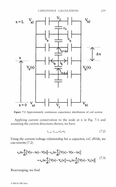
239CAPACITANCE CALCULATIONS
Applying current conservation to the node at x in Fig. 7.1 andassuming the current directions shown, we have
ix-∆x -ix+∆x=ia+ib (7.2)
Using the current-voltage relationship for a capacitor, i=C dV/dt, wecan rewrite (7.2)
(7.3)
Rearranging, we find
Figure 7.1 Approximately continuous capacitance distribution of coil section
© 2002 by CRC Press

CAPACITANCE CALCULATIONS240
(7.4)
Thus the quantity in curly brackets is a constant in time and may for allpractical purposes be set to 0. (For an applied pulse, all the voltages arezero after a very long time so the constant must be zero.) Dividing (7.4)by (∆x)2, we obtain
(7.5)
The first term in (7.5) is the finite difference approximation to d2V/dx2. The combination
(7.6)
can be expressed in terms of the total series capacitance Cs and totalshunt capacitances Ca and Cb using
(7.7)
where N is the number of subdivisions of the total length L into units ofsize ∆x, N=L/∆x Hence (7.7) becomes
(7.8)
Substituting into (7.6), we obtain
(7.9)
© 2002 by CRC Press
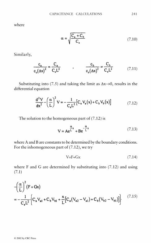
241CAPACITANCE CALCULATIONS
where
(7.10)
Similarly,
(7.11)
Substituting into (7.5) and taking the limit as ∆x→0, results in thedifferential equation
(7.12)
The solution to the homogeneous part of (7.12) is
(7.13)
where A and B are constants to be determined by the boundary conditions.For the inhomogeneous part of (7.12), we try
V=F+Gx (7.14)
where F and G are determined by substituting into (7.12) and using(7.1)
(7.15)
© 2002 by CRC Press

CAPACITANCE CALCULATIONS242
Collecting terms, we find
(7.16)
Thus the general solution to (7.12) is
(7.17)
Using the boundary conditions V=V1 at x=0 and V=V2 at x=L, we cansolve (7.17) for A and B. Performing the algebra, the solution can becast in the form
where
(7.19)
so that γa+γb=1. The derivative of this expression is also needed forevaluating the energy and for obtaining turn-turn voltages. It is
(7.20)
© 2002 by CRC Press
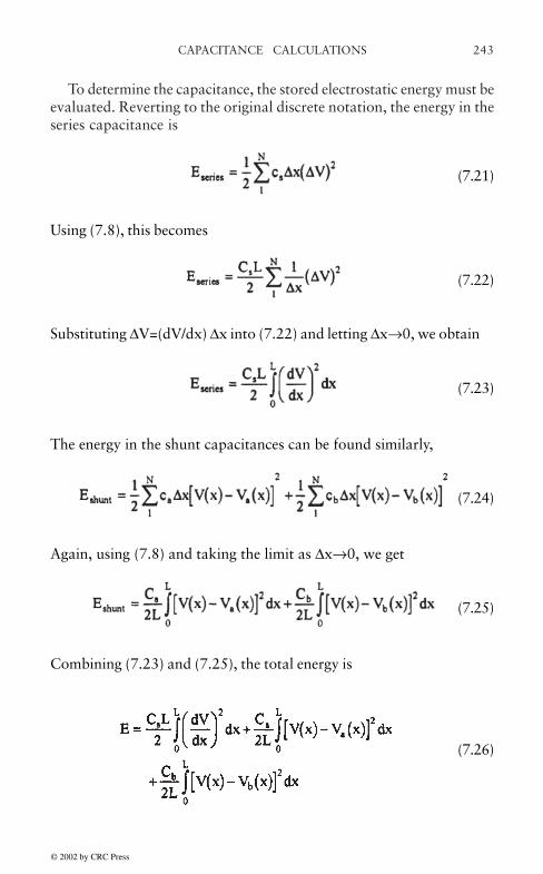
243CAPACITANCE CALCULATIONS
To determine the capacitance, the stored electrostatic energy must beevaluated. Reverting to the original discrete notation, the energy in theseries capacitance is
(7.21)
Using (7.8), this becomes
(7.22)
Substituting ∆V=(dV/dx) ∆x into (7.22) and letting ∆x→0, we obtain
(7.23)
The energy in the shunt capacitances can be found similarly,
(7.24)
Again, using (7.8) and taking the limit as ∆x→0, we get
(7.25)
Combining (7.23) and (7.25), the total energy is
(7.26)
© 2002 by CRC Press

CAPACITANCE CALCULATIONS244
where
(7.28)
For most of the applications of interest here, the side objects onwhich the shunt capacitances terminate are at a constant potential.Thus
(7.29)
and
β=η=γaVa+γbVb (7.30)
We have
(7.31)
(7.32)
(7.33)
Substituting (7.18) and (7.20) into (7.26) and performing theintegrations, we obtain
(7.27)
© 2002 by CRC Press

245CAPACITANCE CALCULATIONS
7.3 STEIN’S CAPACITANCE FORMULA
As an example, we can apply the above results to the case considered byStein, consisting of a disk embedded in a coil of similar disks [Ste64].The situation is shown in Fig. 7.2. Assuming V is the voltage dropacross the disk, we can take V1=V and V2=0. Assuming neighboringdisks have the same voltage drop, we can imagine equipotential planesbetween the disks with the values shown in the figure, namely Va=V andVb=0. As we move along the disk, these values are the average of thetwo potential values on the neighboring disks and can be taken asrepresenting the potential value midway between them. The capacitancesto the mid-plane are twice the disk-disk capacitance, Ca=Cb=2Cdd. Wealso have β=V/2. For these values, the energy, from (7.33), becomes
(7.34)
The effective disk capacitance is found from E=1/2 CV2 and is
(7.35)
where Cs is the series capacitance of the turns,
(7.36)
and Cdd is the disk-disk capacitance.
© 2002 by CRC Press

CAPACITANCE CALCULATIONS246
Let us compare this result with the more conventional approach.This assumes that the voltage drop along the disk is linear so that
(7.37)
The energy in the series turns is, from (7.23)
(7.38)
We must consider the shunt energy with respect to the equipotentialmidplanes as before since we want the energy associated with a singledisk. This is
(7.39)
Figure 7.2 Disk embedded in a coil of similar disks with V the voltage drop along adisk
© 2002 by CRC Press

247CAPACITANCE CALCULATIONS
Evaluating this expression, we find
(7.40)
Combining (7.38) and (7.40) and extracting the effective diskcapacitance, we obtain
(7.41)
This expression applies to a helical winding (one turn/disk) with Cs=0.In order to compare (7.35) with (7.41), let us normalize by dividing
by Cs. Thus
(7.42)
and
(7.43)
From (7.36), the right hand side of (7.42) is a function of Cdd/Cs as is theright hand side of (7.43). Alternatively both right hand sides are functionsof α. For small α, it can be shown that (7.42) approaches (7.43). Forlarger α, the comparison is shown graphically in Fig. 7.3. The differencebecomes noticeable at values of α>5. At α=10, the conventionalcapacitance is about 15% larger than Stein’s.
© 2002 by CRC Press

CAPACITANCE CALCULATIONS248
The voltage distribution along the disk can be obtained from (7.31),substituting V1=V, V2=0, and β=V/2,
(7.44)
This is plotted in Fig. 7.4 in normalized form. As can be seen, thevoltage becomes increasingly less uniform as α increases.
The voltage gradient is obtained from (7.32) with the appropriatesubstitutions and is
(7.45)
This is always negative as Fig. 7.4 indicates. Its largest value, in absoluteterms, occurs at either end of the disk
Figure 7.3 Comparison of Stein’s and conventional capacitance formulas
© 2002 by CRC Press
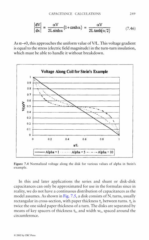
249CAPACITANCE CALCULATIONS
(7.46)
As α→0, this approaches the uniform value of V/L. This voltage gradientis equal to the stress (electric field magnitude) in the turn-turn insulation,which must be able to handle it without breakdown.
In this and later applications the series and shunt or disk-diskcapacitances can only be approximated for use in the formulas since inreality, we do not have a continuous distribution of capacitances as themodel assumes. As shown in Fig. 7.5, a disk consists of Nt turns, usuallyrectangular in cross-section, with paper thickness τp between turns. τp istwice the one sided paper thickness of a turn. The disks are separated bymeans of key spacers of thickness τks and width wks spaced around thecircumference.
Figure 7.4 Normalized voltage along the disk for various values of alpha in Stein’sexample.
© 2002 by CRC Press
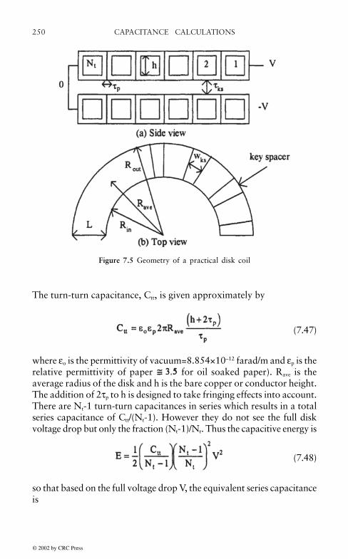
CAPACITANCE CALCULATIONS250
The turn-turn capacitance, Ctt, is given approximately by
(7.47)
where εo is the permittivity of vacuum=8.854×10⁻¹² farad/m and εp is therelative permittivity of paper for oil soaked paper). Rave is theaverage radius of the disk and h is the bare copper or conductor height.The addition of 2τp to h is designed to take fringing effects into account.There are Nt-1 turn-turn capacitances in series which results in a totalseries capacitance of Ctt/(Nt-1). However they do not see the full diskvoltage drop but only the fraction (Nt-1)/Nt. Thus the capacitive energy is
(7.48)
so that based on the full voltage drop V, the equivalent series capacitanceis
Figure 7.5 Geometry of a practical disk coil
© 2002 by CRC Press

251CAPACITANCE CALCULATIONS
(7.49)
This makes sense because for Nt=1, we get Cs=0.The disk-disk capacitance can be considered to be two capacitances
in parallel, namely the capacitance of the portion containing the keyspacers and the capacitance of the remainder containing an oil or airthickness instead of key spacers. Let fks be the key spacer fraction,
(7.50)
where Nks is the number of key spacers spaced around the circumferenceand Wks, their width. Typically fks≈1/3. The key spacer fraction of thedisk-disk space is filled with 2 dielectrics, paper and pressboard, thelatter being the usual key spacer material. For a planar capacitorcontaining 2 dielectric layers of permittivity ε1 and ε2, it follows fromelectrostatic theory that the capacitance is
(7.51)
where A is the area and 1 and 2 are the thicknesses of the layers.Applying this to the disk-disk capacitance, we obtain
(7.52)
Here εks is the permittivity of the key spacer material (=4.5 for oil soakedpressboard) and εoil is the oil permittivity (=2.2 for transformer oil). Rin
and Rout are the inner and outer radii of the disk respectively.
© 2002 by CRC Press
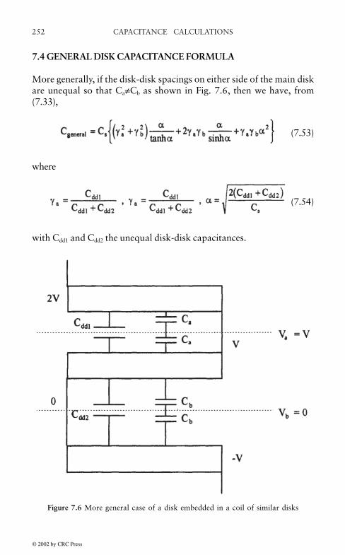
CAPACITANCE CALCULATIONS252
7.4 GENERAL DISK CAPACITANCE FORMULA
More generally, if the disk-disk spacings on either side of the main diskare unequal so that Ca≠Cb as shown in Fig. 7.6, then we have, from(7.33),
(7.53)
where
(7.54)
with Cdd1 and Cdd2 the unequal disk-disk capacitances.
Figure 7.6 More general case of a disk embedded in a coil of similar disks
© 2002 by CRC Press

253CAPACITANCE CALCULATIONS
7.5 COIL GROUNDED AT ONE END WITH GROUNDEDCYLINDERS ON EITHER SIDE
An early impulse model for a coil assumed the coil consisted of auniformly distributed chain of series capacitances connected to groundcylinders on either side by shunt capacitances, i.e. the same model shownin Fig. 7.1 but with Va1=Va2=Vb1=Vb2=0 [Blu51]. The V1 terminal wasimpulsed with a voltage V and the V2 terminal was grounded. From(7.30) we have β=η=0 and (7.31) becomes
(7.55)
with . Here Cg is the total ground capacitance (both sides)and Cs the series capacitance of the coil. This is shown in normalizedform in Fig. 7.7 for several values of α.
Figure 7.7 Graph of normalized voltage along a coil for several values of α
© 2002 by CRC Press

CAPACITANCE CALCULATIONS254
This voltage distribution is expected to apply immediately after theapplication of the impulse voltage, before inductive effects come intoplay. Later, oscillations can cause voltage swings above the valuesshown in the figure.
The voltage gradient is given by
(7.56)
The maximum gradient occurs at the line end (x=0) and is
(7.57)
Thus the maximum disk-disk voltage immediately after impulse isapproximately (7.57) multiplied by the disk-disk spacing.
The coil’s total capacitance to ground is, from (7.33),
(7.58)
In this as well as previous formulas in this section, the series capacitanceis due to Nd disks in series and if the disk capacitances are obtained bythe Stein formula, we have
(7.59)
For an inner coil, the surfaces of the neighboring coils are usually takento be the ground cylinders. For the innermost coil, the core determinesthe ground on one side while for an outermost coil the tank is the groundon one side. In general, the distance to ground is filled with variousdielectric materials, including oil or air. One such structure is shown inFig. 7.8. There are usually multiple pressboard layers, but forconvenience there are grouped into a single layer.
The sticks provide spacing for cooling oil or air to flow. Thiscomposite structure is similar to that analyzed previously for the disk-disk capacitance. The ground spacing is usually small relative to thecoil radius for power transformers so that an approximately planar
© 2002 by CRC Press
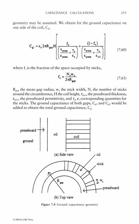
255CAPACITANCE CALCULATIONS
geometry may be assumed. We obtain for the ground capacitance onone side of the coil, Cg1
(7.60)
where fs is the fraction of the space occupied by sticks,
(7.61)
Rgap the mean gap radius, ws the stick width, Ns the number of sticksaround the circumference, H the coil height, τpress the pressboard thickness,εpress the pressboard permittivity, and τs, εs corresponding quantities forthe sticks. The ground capacitance of both gaps, Cg1 and Cg2 would beadded to obtain the total ground capacitance, Cg.
Figure 7.8 Ground capacitance geometry
© 2002 by CRC Press

CAPACITANCE CALCULATIONS256
7.6 STATIC RING ON ONE SIDE OF DISK
If a static ring is present on one side of a disk and connected to theterminal voltage as shown in Fig. 7.9, then we have a situation similarto that considered in the general disk capacitance section. The onlydifference is that Ca is the disk-static ring capacitance since the staticring is an equipotential surface. Thus (7.53) applies with
(7.62)
with Cdd the disk-disk capacitance to the lower disk.This case would be identical to Stein’s if the static ring were spaced
at 1/2 the normal disk-disk spacing or whatever is required to achieveCa =2Cdd=Cb. Then γa=γb=1/2, and (7.53) would reduce to(7.35). Thus the end disk would have the same capacitance as any otherdisk.
Figure 7.9 Static ring on one side of a disk at the end of a coil
© 2002 by CRC Press
257CAPACITANCE CALCULATIONS
7.7 TERMINAL DISK WITHOUT A STATIC RING
In case the end disk does not have an adjacent static ring, we assumethat the shunt capacitance on the end side is essentially 0. Then we havethe situation shown in Fig. 7.10a. We have Ca=0 so that γa=0 , γb=1 andfrom (7.53)
(7.63)
with
(7.64)
This situation also applies to a center fed winding without staticring. In this case, as Fig. 7.10b shows, there is no capacitative energybetween the two center disks so that effectively Ca=0. This result wouldalso follow if both center disks were considered as a unit and the energydivided equally between them.
© 2002 by CRC Press

CAPACITANCE CALCULATIONS258
7.8 CAPACITANCE MATRIX
Before proceeding to other cases of interest, we need to introduce thecapacitance matrix. For a system of conductors having voltages Vi andtotal electrostatic energy E, it follows from the general theory of linearcapacitors that [Smy68]
Figure 7.10 Terminal disk without a static ring
© 2002 by CRC Press
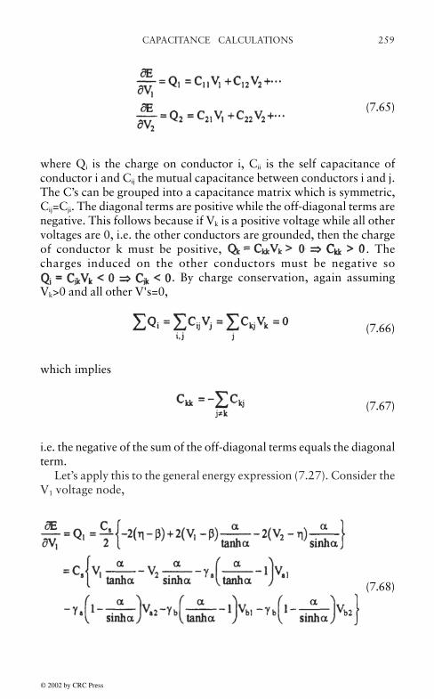
259CAPACITANCE CALCULATIONS
(7.65)
where Qi is the charge on conductor i, Cii is the self capacitance ofconductor i and Cij the mutual capacitance between conductors i and j.The C’s can be grouped into a capacitance matrix which is symmetric,Cij=Cji. The diagonal terms are positive while the off-diagonal terms arenegative. This follows because if Vk is a positive voltage while all othervoltages are 0, i.e. the other conductors are grounded, then the chargeof conductor k must be positive, . Thecharges induced on the other conductors must be negative so
. By charge conservation, again assumingVk>0 and all other V's=0,
(7.66)
which implies
(7.67)
i.e. the negative of the sum of the off-diagonal terms equals the diagonalterm.
Let’s apply this to the general energy expression (7.27). Consider theV1 voltage node,
(7.68)
© 2002 by CRC Press

CAPACITANCE CALCULATIONS260
Using the labeling scheme 1, 2, 3, 4, 5, 6↔1, 2, a1, a2, b1, b2, theoff-diagonal mutual capacitances are, from (7.68)
(7.69)
These are all negative and the negative of their sum is C11 which is
(7.70)
This is an example of (7.67).The capacitance diagram corresponding to this situation is shown in
Fig. 7.11, which shows only the capacitances attached to voltage nodeV1. The other mutual capacitances can be filled in by a similarprocedure. If the side voltages are constant so that Va1=Va2=Va andVb1=Vb2=Vb, then there is only one mutual capacitance connecting 1 to aand it is given by
(7.71)
and similarly for C1b. For small α, this approaches
(7.72)
so that on the capacitance diagram, 1/2 the shunt capacitance is attachedto the V1 node. If we carried through the analysis, we would find that 1/2 of the shunt capacitance would also be attached to the V2 node,producing a π capacitance diagram.
© 2002 by CRC Press
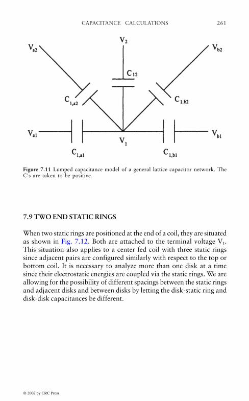
261CAPACITANCE CALCULATIONS
7.9 TWO END STATIC RINGS
When two static rings are positioned at the end of a coil, they are situatedas shown in Fig. 7.12. Both are attached to the terminal voltage V1.This situation also applies to a center fed coil with three static ringssince adjacent pairs are configured similarly with respect to the top orbottom coil. It is necessary to analyze more than one disk at a timesince their electrostatic energies are coupled via the static rings. We areallowing for the possibility of different spacings between the static ringsand adjacent disks and between disks by letting the disk-static ring anddisk-disk capacitances be different.
Figure 7.11 Lumped capacitance model of a general lattice capacitor network. TheC's are taken to be positive.
© 2002 by CRC Press
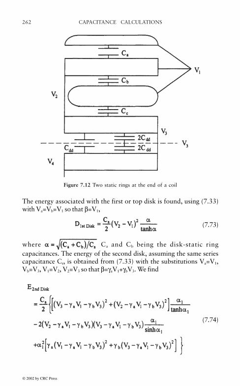
CAPACITANCE CALCULATIONS262
The energy associated with the first or top disk is found, using (7.33)with Va=Vb=V1 so that β=V1,
(7.73)
where Ca and Cb being the disk-static ringcapacitances. The energy of the second disk, assuming the same seriescapacitance Cs, is obtained from (7.33) with the substitutions Va=V1,Vb=V3, V1=V2, V2=V3 so that β=γaV1+γbV3. We find
Figure 7.12 Two static rings at the end of a coil
(7.74)
© 2002 by CRC Press

263CAPACITANCE CALCULATIONS
The lumped capacitance network associated with this configurationcan be obtained by the procedure described in the previous section. Thus
with ,
γa+γb=1, this can be
simplified
(7.75)
(7.76)
Thus the total energy in the first two disks with static rings is
Reading off the mutual capacitances from (7.77), we find
(7.77)
(7.78)
© 2002 by CRC Press

CAPACITANCE CALCULATIONS264
Extracting the mutual capacitances, we find
(7.80)
These are negative and the negative of their sum is C22. Moreover, wesee that C21=C12 as expected since the capacitance matrix is symmetric.Differentiating (7.76) with respect to V3 would give us no newinformation.
Thus we can draw the lumped capacitance diagram for thisconfiguration as shown in Fig. 7.13. We assume the capacitances shownare positive (the negative of the mutual capacitances). Hence the totalcapacitance between the V1 and V3 terminals is given by
(7.81)
These are negative and minus their sum is the self capacitance C11.We also need to find C23. This is obtained by differentiating (7.76)
with respect to V2
(7.79)
© 2002 by CRC Press
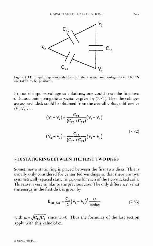
265CAPACITANCE CALCULATIONS
In model impulse voltage calculations, one could treat the first twodisks as a unit having the capacitance given by (7.81), Then the voltagesacross each disk could be obtained from the overall voltage difference(V1-V3)via
(7.82)
7.10 STATIC RING BETWEEN THE FIRST TWO DISKS
Sometimes a static ring is placed between the first two disks. This isusually only considered for center fed windings so that there are twosymmetrically spaced static rings, one for each of the two stacked coils.This case is very similar to the previous case. The only difference is thatthe energy in the first disk is given by
(7.83)
with since Ca=0. Thus the formulas of the last sectionapply with this value of α.
Figure 7.13 Lumped capcitance diagram for the 2 static ring configuration, The C'sare taken to be positive.
© 2002 by CRC Press
CAPACITANCE CALCULATIONS266
7.11 WINDING DISK CAPACITANCES WITH WOUND-IN-SHIELDS
This section is essentially a reprint of our published paper [Del98]. ©1997 IEEE. Reprinted, with permission, from IEEE Trans. on PowerDelivery, Vol. 13, No. 2, pp. 503–509, April 1998.
In order to improve the voltage distribution along a transformer coil,i.e. to reduce the maximum disk-disk voltage gradient, it is necessary tomake the distribution constant, α, as small as possible, where α
with Cg the ground capacitance and Cs the series capacitanceof the coil. One way of accomplishing this is to increase Cs. Commonmethods for increasing the series capacitance include interleaving[Nuy78] and the use of wound-in-shields [For69]. Both of thesetechniques rely on inductive effects. Geometric methods for increasingCs such as decreasing turn-turn or disk-disk clearances are generallyruled out by voltage withstand or cooling considerations.
Interleaving can produce large increases in Cs which may benecessary in very high voltage applications. However, it can be verylabor intensive and in practice tends to be limited to magnet wireapplications. Wound-in-shields tend to produce more modest increasesin Cs compared with interleaving. However, they require less labor andare suitable for use with transposed cable. In addition, they can easilyprovide a tapered capacitance profile to match the voltage stress profileof the winding.
Here we present a simple analytic formula for calculating the diskcapacitance with a variable number of wound-in-shield turns. Since thisformula rests on certain assumptions, a detailed circuit model isdeveloped to test these assumptions. Finally, experiments are carriedout to check the formula under a wide variety of conditions.
7.11.1 Analytic Formula
Fig. 7.14 shows the geometry of a pair of disks containing a wound-in-shield. Also shown is the method of labeling turns of the coil and shield.Since the shield spans two disks, it is necessary to calculate thecapacitance of the pair. Each disk has N turns and n wound-in-shieldturns, where n≤N-1. The voltage across the pair of disks is V and weassume the rightmost turn of the top disk, i=1, is at voltage V and therightmost turn of the bottom disk, j=1, is at 0 volts, so that the coil is
© 2002 by CRC Press

267CAPACITANCE CALCULATIONS
We assume the voltage rise per turn is ∆V where
(7.84)
We assume this same volts per turn applies to the shield as well. Fordefmiteness, we assume the voltage at the shield cross-over point isVbias as shown in Fig. 7.14. Taking the voltage at the midpoint of aturn, we have for the top disk
Vc(i)=V-(i-0.5)∆V (7.85)
where Vc(i) is the coil voltage for turn i, i=1,…, N. Also for the top disk
Vw(i)=Vbias-(i-0.5)∆V (7.86)
where Vw(i) is the shield voltage for turn i, i=1,…, n. For the bottomdisk, we have
wound in a positive sense from outer to inner turn on the bottom diskand from inner to outer turn on the top disk. The shield turns are placedbetween the coil turns and are wound in the same sense as the coil.However, their cross-over is at the outermost turn rather than theinnermost one as is the case for the coil. This means that the positivevoltage sense for the shield is from the leftmost turn, i=n , on the top coilto turn i=1 on the top disk and then from turn j=1 to j=n on the bottomdisk.
Figure 7.14 Disk pair with wound-in-shields with labelling and other parametersindicated
© 2002 by CRC Press

CAPACITANCE CALCULATIONS268
Vc(j)=V+(j-2N-0.5)∆V (7.87)
for j=1,…, N and
Vw(j)=Vbias+(J-0.5)∆V (7.88)
for j=1,…, n.Letting cw be the capacitance between a coil turn and adjacent shield
turn, the energy stored in the capacitance between shield turn i and itsadjacent coil turns is
(7.89)
The two terms reflect the fact that there are two adjacent coil turns forevery shield turn. Using the previous expressions for the V's, (7.89)becomes
(7.90)
This does not depend on i and so is the same for all n shield turns on thetop disk. For the bottom disk, (7.89) applies with j replacing i so thecapacitative energy between shield turn j and its surrounding coil turnsis
(7.91)
This again does not depend on j and so is the same for all n shield turnson the bottom disk.
To the above energies, we must add the capacitative energy of theturns without wound-in-shields between them. Letting ct be the turn-turncapacitance, this energy is simply
(7.92)
There are 2(N-n-1) such terms in the energy. In addition, there is energystored in the disk-disk capacitance, cd . Since we are assuming the voltage
© 2002 by CRC Press
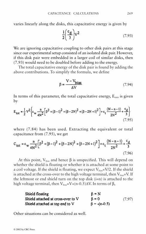
269CAPACITANCE CALCULATIONS
varies linearly along the disks, this capacitative energy is given by
(7.93)
We are ignoring capacitative coupling to other disk pairs at this stagesince our experimental setup consisted of an isolated disk pair. However,if this disk pair were embedded in a larger coil of similar disks, then(7.93) would need to be doubled before adding to the energy.
The total capacitative energy of the disk pair is found by adding theabove contributions. To simplify the formula, we define
(7.94)
In terms of this parameter, the total capacitative energy, Etot, is givenby
where (7.84) has been used. Extracting the equivalent or totalcapacitance from (7.95), we get
At this point, Vbias and hence β is unspecified. This will depend onwhether the shield is floating or whether it is attached at some point toa coil voltage. If the shield is floating, we expect Vbias=V/2. If the shieldis attached at the cross-over to the high voltage terminal, then Vbias=V. Ifthe leftmost or end shield turn on the top disk (i=n) is attached to thehigh voltage terminal, then Vbias=V+(n-0.5)∆V. In terms of β,
(7.95)
(7.96)
Other situations can be considered as well.
(7.97)
© 2002 by CRC Press

CAPACITANCE CALCULATIONS270
For the turn-turn capacitance, we used the expression (in SI units)
(7.98)
where Rave is the average radius of the coil, h the bare copper height ofa coil turn in the axial direction, τc the 2-sided paper thickness of a coilturn, εo=8.85×10⁻¹²F/m, and εp the relative permittivity of paper. Theaddition of 2τc to h is designed to take fringing effects into account. Alsothe use of Rave is an approximation which is reasonably accurate forcoils with radial builds small compared with their radii. For thecapacitance cw the same expression was used but with τc replaced by0.5(τc+τw) where τw is the 2-sided paper thickness of a shield turn. Sincethere are key spacers separating the disks and gaps between them, thedisk-disk capacitance is given by
(7.99)
where Ri and Ro are the inner and outer radii of the disk respectively, fis the fraction of the disk-disk space occupied by key spacers, τk is thekey spacer thickness, εk the key spacer relative permittivity, and εa therelative permittivity of air (=1) since the coils were tested in air.
7.11.2 Circuit Model
Since quite a few assumptions went into deriving the capacitance formulain the last section, we decided to model the disk pair by means of acircuit model, including capacitative, inductive, and resistive effects assketched in Fig. 7.15. We include all mutual couplings between theturns of the coil and wound-in-shield. The circuit is assumed to beexcited by a current source which is nearly a step function. The circuitequations are
(7.100)
© 2002 by CRC Press

271CAPACITANCE CALCULATIONS
where C is a capacitance matrix, M an inductance matrix, R a diagonalresistance matrix and A, B matrices of ±1's and 0's. The voltage andcurrent vectors, V and I, include the coil and shield turn voltages andcurrents. These equations are solved by means of a Runge-Kutta solver.
Figure 7.15 Circuit model for a disk pair with wound-in-shields. The labelling schemeand circuit parameters are indicated.
© 2002 by CRC Press

CAPACITANCE CALCULATIONS272
Since the experimental setup was in air, we used air core inductanceand mutual inductance expressions. The mutual inductance betweentwo thin wire coaxial loops of radii r1 and r2 spaced a distance d apartis given by [Smy68] in MKS units,
(7.101)
K(k) and E(k) are complete elliptic integrals of the first and second kindsrespectively and µo=4π×10–7 H/m. For rectangular cross-section coils,Lyle’s method in conjunction with (7.101) could be used for a moreaccurate determination of the mutual inductance [Gro73]. However, forthe turn-turn mutual inductances in our experimental coils, treating theturns as thin circular loops was nearly as accurate as Lyle’s method.The self inductance of a single turn circular coil of square cross sectionwith an average radius of a and square side length c is given by [Gro73]in MKS units
(7.102)
This applies for c/2a≤0.2. When the cross-section is not square, it can besubdivided into a number of squares and (7.102) together with (7.101)can be applied to compute the self inductance more accurately. In ourexperimental coil, the turn dimensions were such that the simple formulawith c taken as the square root of the turn area agreed well with themore accurate calculation,
The turn-turn and turn-shield capacitances were the same as given inthe last section. The capacitance Cb in Fig. 7.15 was taken as Cd/N. Wedid not include the capacitance between shield turns on neighboringdisks in our final calculations. Their inclusion had little effect on thetotal capacitance.
The resistances used in the circuit model were based on the wiredimensions but were multiplied by a factor to account for high
© 2002 by CRC Press

273CAPACITANCE CALCULATIONS
frequency This factor may be estimated by examining the frequencydependence of the two main contributors to the coil loss, namely theJoule or I2R loss and the eddy current loss due to stray flux carried bythe conductor strands. Based on a formula in Ref. [Smy68] forcylindrical conductors, the Joule loss is nearly independent of frequencyat low frequencies which includes 60 Hz for our conductor dimensions.At high frequencies, the loss divided by the dc or 60 Hz loss is given by,
(7.103)
where rcond is the radius of the conductor or in our case an effectiveradius based on the wire dimensions, σ is the wire’s conductivity, and fin this context is the frequency in Hz. Based on our cable dimensionsand for a typical frequency encountered in our calculations andexperiment of ~0.15 MHz, we estimate that Wjoule(f)/WJoule(f=0)~ 15.9The eddy current frequency dependence due to stray flux is given inRef. [Lam66]. At low frequencies, this loss varies as f2 whereas at highfrequencies, it varies as f0.5. Taking ratios of the high to low frequencyeddy current loss, we obtain
(7.104)
where b is the thickness of the lamination or strand in a directionperpendicular to the stray magnetic field. In our case, the cable wasmade of rectangular strands with dimensions 0.055 in.×0.16 in. (1.4mm×4.06 mm). For the small dimension, (7.104) gives a ratio of 68,086while for the large dimension, we get a ratio of 2,766. A detailed fieldmapping is necessary to obtain the eddy current loss contribution at lowfrequencies but typically this amounts to about 10% of the dc loss,depending on the cable construction. If we assume that the small andlarge dimension eddy losses are equal at low frequencies, i.e. each is5% of the dc loss, then we find that the ratio of high to low frequencytotal loss based on the above ratios is given by Wtot(f)/Wtot(60Hz)=3557,This is only a crude estimate. Our data show that this ratio is about1500 for our cable. Since the capacitance obtained from the simulationis nearly independent of the resistance used, we did not try to match themodel’s resistance with the experimental values. A sample output isshown in Fig. 7.16.
© 2002 by CRC Press

CAPACITANCE CALCULATIONS274
Two methods were used to extract the equivalent total capacitancefrom the circuit model. Since the voltages of each coil and shield turnwere determined at each time step, the capacitive energy was simplysummed and the total capacitance determined via
(7.105)
where V is the voltage of turn i=1 at the particular time step. At the endof the total time duration of about 200 time steps, the average andmedian total capacitances were calculated. These two values generallyagreed fairly closely. The other method consisted of extracting the totalcapacitance from a simplified equivalent circuit as shown in Fig. 7.17.This latter method was also used to obtain the total capacitanceexperimentally.
Figure 7.16 Voltage across the coil pair versus time from the detailed circuit modelcalcualtions.
© 2002 by CRC Press

275CAPACITANCE CALCULATIONS
for t≥0. Here
(7.107)
In the limiting case as R→0, (7.106) becomes
(7.108)
In all the cases examined computationally or experimentally, theterm (R/2L)2 was much smaller than 1/LC so that it can be ignored inthe expression for ωo. Thus by measuring the oscillation frequency, wedetermine the combination LC, To obtain C, an additional capacitance,
Figure 7.17 Simplified circuit model for capacitance determination
Using Laplace transforms, the circuit of Fig. 7.17 can be solvedanalytically, assuming a step function current input of magnitude I. Weobtain
(7.106)
© 2002 by CRC Press

CAPACITANCE CALCULATIONS276
C1, was placed in parallel with the coil and a new oscillation frequency,ω1, determined. Since this added capacitance doesn’t change L, wehave, taking ratios and squaring (7.107),
(7.109)
Since ωo and ω1 can be measured or determined from the output of thecircuit model and C1 is known, C can be obtained. We found goodagreement between the two methods of determining C.
7.11.3 Experimental Methods
A coil containing two disk sections was made of transposed cable. Therewere 10 turns per disk. The cable turns were 0.462 in. radial build by0.362 in. axial height, including a 30 mil (2-sided) paper cover (1.17cm ×0.919 cm with 0.76 mm paper). The inner radius was 9.81 in.(0.249 m). The outer radius depended on the number of shield turns butwas approximately 15.4 in. (0.392 m). The wound-in-shield turnsconsisted of 0.14 in. radial build by 0.365 in. axial height magnet wire,including a 20 mil (2-sided) paper cover (0.355 cm×0.927 cm with 0.51mm paper). The disks were separated by means of 18 key spacers equallyspaced around the circumference. The key spacers were 1.75 in wide by0.165 in. thick (4.45 cm×0.419 cm).
The coil was excited by means of a current source which produced anear step function current. A sample of the current input and coilvoltage output is shown in Fig. 7.18. This voltage vs time plot wasFourier analyzed to extract the resonant frequency. Frequencies weremeasured with and without an external capacitor of 10 nF across thecoil in order to obtain the coil capacitance by the ratio methoddescribed previously.
Shield turns/disk of n=3, 5, 7, 9 were tested as well as the no shieldcase, n=0. In addition, for each n value, tests were performed with theshield floating, attached to the high voltage terminal at the cross-over,and attached to the high voltage terminal at the end shield turn on thetop disk. Other methods of attachment were also made for the n=9 caseto test for expected symmetries.
Because the disk pair was not contained in a tightly wound coil,there tended to be some looseness in the winding. This could bedetermined by squeezing the disk turns tightly together and noting howmuch the radial build decreased. From this we could determine how
© 2002 by CRC Press
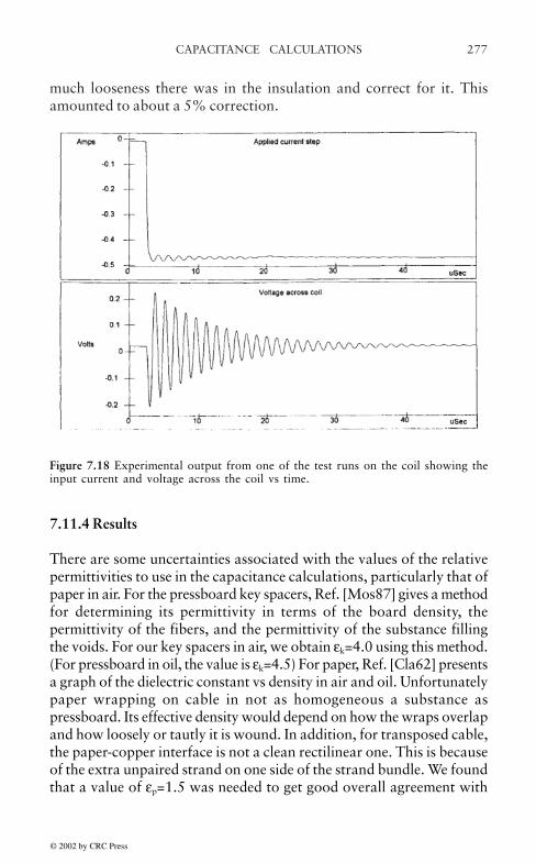
277CAPACITANCE CALCULATIONS
much looseness there was in the insulation and correct for it. Thisamounted to about a 5% correction.
7.11.4 Results
There are some uncertainties associated with the values of the relativepermittivities to use in the capacitance calculations, particularly that ofpaper in air. For the pressboard key spacers, Ref. [Mos87] gives a methodfor determining its permittivity in terms of the board density, thepermittivity of the fibers, and the permittivity of the substance fillingthe voids. For our key spacers in air, we obtain εk=4.0 using this method.(For pressboard in oil, the value is εk=4.5) For paper, Ref. [Cla62] presentsa graph of the dielectric constant vs density in air and oil. Unfortunatelypaper wrapping on cable in not as homogeneous a substance aspressboard. Its effective density would depend on how the wraps overlapand how loosely or tautly it is wound. In addition, for transposed cable,the paper-copper interface is not a clean rectilinear one. This is becauseof the extra unpaired strand on one side of the strand bundle. We foundthat a value of εp=1.5 was needed to get good overall agreement with
Figure 7.18 Experimental output from one of the test runs on the coil showing theinput current and voltage across the coil vs time.
© 2002 by CRC Press

CAPACITANCE CALCULATIONS278
the test data. This would correspond to an effective paper density of 0.5gm/cm3 according to the graph in Ref. [Cla62]. At that density, paper inoil would have εp=3.0 according to the same graph. For tightly woundpaper in oil, values of εp=3.5–4.0 are typically used. Thus a paperpermittivity of 1.5 for paper in air is not unreasonable.
Table 7.1 shows the test results along with the calculated values ofthe capacitance for different numbers of shield turns and different shieldbiasing. The overall agreement is good. Certainly the trends are wellreproduced. Even for the floating shield case which has the lowestcapacitative enhancement, there is a capacitance increase of a factor of5 for 3 shield turns/disk and a factor of about 13 for 9 shield turns/diskover the unshielded case. By biasing the shield in different ways, evengreater increases are achieved.
In Table 7.2, the coil turn and shield turn voltages as calculated bythe circuit model at time t=30 µsec are shown for the n=9 case with theshields floating. As can be seen, the coil volts/turn is about the same asthe shield volts/turn, verifying the assumption made in the analytic
Table 7.1 Capacitance of coil with 2 disks of 10 turns/disk and variable number ofwound-in-shield turns/disk.
© 2002 by CRC Press

279CAPACITANCE CALCULATIONS
model. In addition, VbiasH≈V/2 as was also assumed in the simplemodel. Also the voltage differences between the coil and shield turnsfall into two groups of either ~12.8 or 11.5 V in this case. This alsocorresponds to the simple model prediction of either N∆V=V/2 or (N-1)∆V=V/2-∆V volts. Thus, in the case where the shields are floating, themaximum turn-shield voltage is V/2. Based on the simple model, thisholds regardless of the number of shield turns.
In Table 7.3, we show the corresponding output from the circuitmodel at t=150 µsec for the case where the shield is attached at thecross-over to the high voltage terminal. (It was actually attached toshield turn i=1 in the model.) We see again that the coil volts/turn≈shield volts/turn. According to the simple model prediction (β=0), the
Table 7.2 Turn voltages at t=30 µsec for a coil of 2 disks with 10 turns/disk and 9shield turns/disk with the shield floating.
© 2002 by CRC Press

CAPACITANCE CALCULATIONS280
to the high voltage terminal could be analyzed similarly although thisconfiguration is harder to achieve in practice. This configuration alsohas a higher coil turn to shield turn voltage difference than the othermethods of shield attachment. As expected, however, the price to pay
voltage differences between shield and adjacent turn on the top disk are0 and ∆V as is also nearly the case for the circuit model. Along thebottom disk, the simple model gives voltage differences of 2N∆V=V and(2N-1) ∆V=V-∆V and this is also nearly the case for the circuit model.Thus the maximum coil turn to shield turn voltage is V. According tothe simple model, this holds regardless of the number of shield turns.
The case where the end turn of the shield on the top disk is attached
Table 7.3 Turn voltages at t=150 µsec for a coil of 2 disks with 10 turns/disk and 9shield turns/disk with the shield attached at the cross-over to the high voltageterminal.
© 2002 by CRC Press

281CAPACITANCE CALCULATIONS
for the higher capacitances are higher coil turn to shield turn voltagedifferences.
Several symmetric situations were noted in the experimental data.These symmetries were only checked for the n=9 case but should applyto all n values according to the simple model. We found that attachingthe high voltage terminal to the end shield turn on the top disk (i=n)produced the same capacitance as attaching the low voltage terminal,at 0 volts here, to the end turn on the bottom disk (j=n). This symmetrycan be seen in the simple formula (7.96) by using the appropriate valuesfor β. Attaching the top end shield turn to the low voltage terminalproduced the same capacitance as attaching the bottom end shield turnto the high voltage terminal. This can also be shown by means of thesimple formula. Also the same capacitance was produced whether theshield cross-over was attached to the high or low voltage terminal. Thisalso follows from the simple model.
For consistency, the inductance of our coil was extracted from theexperimental data as well as from the circuit model output. We foundL(data)=280 µH and L(circuit model)=320 µH. Using an algorithm inGrover [Gro73], we obtained L(calc)=340 µH. These are all withinreasonable agreement. The decay constant R/2L appearing in (7.106)could be extracted from the data by analyzing the envelope of thedamped sinusoid (Fig. 7.18) and we found that it could be dropped inthe formula for ωo (7.107). We also observed a significant resistancechange when the frequency was changed by adding the externalcapacitance.
7.12 MULTI-START WINDING CAPACITANCE
Multi-start windings are a simple example of an interleaved type ofwinding. They are commonly used as tap windings. In these windings,adjacent turns have voltage differences which can differ from the usualturn-turn voltage drop along typical disk or helical windings. Althoughmulti-start windings are helical windings, they can be thought of as acollection of superposed series connected helical windings as shown inFig. 7.19.
© 2002 by CRC Press

CAPACITANCE CALCULATIONS282
These winding essentially start over again and again whichmotivates the name. Each start represents a constitutent winding havinga certain number of turns called turns per start. The number of starts isthe same as the number of constituent windings. By connecting tapsbetween the starts, the turns per start become the number of tap turns.Their advantage as tap windings compared with the standard type isthat they allow a more balanced force distribution regardless of the tapsetting and do not require thinning of adjacent windings.
Although shown as side by side windings in the figure forexplanatory purposes, the windings are superposed into one helical typeof winding. The botton to top connections are made external to thiswinding. The constituent windings are meshed in such a way that thevoltage difference between adjacent turns in the composite winding iskept to one or two times the voltage drop along a constituent windingwhich is really the best that can be done. Letting 1, 2, 3,…label turnsfrom the different constituent windings, acceptable meshing schemesare shown in Fig. 7.20 for various numbers of starts, Ns,
Figure 7.19 Schematic illustration of a multi-start winding
© 2002 by CRC Press

283CAPACITANCE CALCULATIONS
The turns are arranged along the winding according to Fig. 7.20.The voltage differences between adjacent turns, measured in units of thevoltage drop between starts, are also indicated in the figure. A patterncan be seen in the organization: Start with turn 1 from start coil 1. Putturn 2 from start coil 2 at the end of the group. Put turn 3 from start coil3 below turn 1. Put turn 4 from start coil 4 above turn 2. Put turn 5 fromstart coil 5 below turn 3. Put turn 6 from start coil 6 above turn 4. Etc.until you run out of start coils. Then repeat the pattern until you run outof turns in the start coils.
The capacitance is obtained by summing up the capacitative energyassociated with the winding configuration. Letting ctt be the turn to turncapacitance and ∆Vtt the voltage difference between turns, the energyassociated with a pair of adjacent turns is given by Energy(turn-turn)=1/2 ctt(∆Vtt)2. Letting the voltage drop between starts be ∆Vs, the totalenergy is obtained by summing all the turn-turn energies. As can beseen, each group of turns has two 1's except for the last group which hasonly 1. If there are n turns/start, there are n such groups. Hence the
Figure 7.20 Winding schemes for multi-start windings. The numbers beside the turnsare the voltage differences between turns in units of the voltage drop between starts.
© 2002 by CRC Press
CAPACITANCE CALCULATIONS284
energy is 2n-1 times the energy associated with voltage ∆Vs acrosscapacitance ctt. The remaining turn-turn voltages in the group have avoltage of 2×∆Vs across them. There are Ns-2 such turns in the group.Since there are n such groups, the energy associated with these isn×(Ns∆2) times the energy associated with a voltage of 2∆Vs acrosscapacitance ctt. Combining these energies, we get at total energy of
(7.110)
Since ∆Vs=V/Ns, where V is the total energy across the entire winding,by substituting this into (7.110), we can extract a total capacitance forthe winding, Cm-s,
(7.111)
ctt will depend on the insulation structure of the winding, i.e. whetherthe turns are touching, paper to paper, in the manner of a layer windingor whether there is an oil gap separating them. In any event, thecapacitance is much higher than that across a comparable helical windingwhere the turn-turn voltages are much smaller.
© 2002 by CRC Press

285
8. HIGH VOLTAGE INSULATIONDESIGN
Summary Transformer insulation must not only be designed to withstandthe normal operating voltages but to survive the effects of lightningstrikes and other possible disturbances such as switching operations whichmay occur on the electrical system. In order to assess the adequacy ofthe insulation, it is necessary to have some understanding of thebreakdown process, especially in liquids and solids which are normallyused in combination in large power transformers. Although ourunderstanding in this area is very incomplete, some trends or correlationshave been deduced from test data. Using these and much accumulatedexperience, design rules have been formulated whose main justificationis that they work in practice at least in most cases. It is also necessary tohave some means of calculating the voltages and electric stresses whichoccur in a transformer under normal and especially abnormal conditionssuch as lighting strikes. From such calculations, voltages, voltagedifferences, and electrical stresses can be obtained and compared withthe breakdown limits. Although a standardized waveform has beendeveloped to represent a typical lightning strike which reaches atransformer, simple step function approximations are often used inapproximate analytical calculations. The test of design adequacy comeswhen the unit is built and is subjected to a variety of electrical tests tosimulate the abnormal conditions. The ultimate test comes from theunit’s survival in service for long periods of time.
8.1 INTRODUCTION
A transformer’s insulation system must be designed to withstand notonly the a.c. operating voltages, with some allowance for an ~15%overvoltage, but also the much higher voltages produced by lightningstrikes or switching operations. These latter voltages can be limited byprotective devices such as lightning or surge arresters but these devicesare usually set to protect at levels well above the normal a.c. operatingvoltage. Fortunately the transformer’s insulation can withstand highervoltages for the shorter periods of time characteristic of lightning orswitching disturbances. Thus, insulation designed to be adequate at the
© 2002 by CRC Press

HIGH VOLTAGE INSULATION DESIGN286
operating voltage can also be sufficient for the short duration highervoltages which may be encountered.
Insulation design is generally an iterative process. A particularwinding type is chosen such as disk, helix, or layer, for each of thetransformer’s windings. They must have the right number of turns toproduce the desired voltage and must satisfy thermal, mechanical, andimpedance requirements. The voltage distribution is then calculatedthroughout the windings, using a suitable electrical model together withthe appropriate input such as a lightning impulse excitation. Voltagedifferences and/or electric fields are then calculated to determine if theyare high enough to cause breakdown, according to some breakdowncriterion, across the assumed insulation structure. More elaborate pathintegrals are sometimes used to determine breakdown. If the breakdowncriterion is exceeded at some location, the insulation is redesigned andthe process repeated until the breakdown criteria are met. Insulationredesign can consist of adding more paper insulation to the wire or cable,increasing the size of the oil or air ducts, or resorting to interleaving thewinding conductors or adding wound-in-shields or other types of shields.
Although voltages and electric fields can be calculated to almost anydesired accuracy, assuming the material properties are well known, thesame cannot be said for breakdown fields in solids or liquids. Thetheory of breakdown in gases is reasonably well established, but thesolid or liquid theory of breakdown is somewhat rudimentary.Nevertheless, design rules have evolved based on experience. Withsuitable margins, these rules generally produce successful designs.Success is usually judged by whether a transformer passes a series ofdielectric tests using standard impulse waveforms or a.c. powerfrequency voltages for specified time periods without breakdown orexcessive corona. These tests have been developed over the years in aneffort to simulate a typical lightning or switching waveshape.
8.2 PRINCIPLES OF VOLTAGE BREAKDOWN
We briefly discuss some of the proposed mechanisms of voltagebreakdown in solids, liquids, and gases with primary emphasis ontransformer oil. This is because in oil filled transformers, due to thehigher dielectric constant of the solid insulation, the highest electricstress tends to occur in the oil. In addition, the breakdown stress of theoil is generally much lower than that of the solid insulation. The samesituation occurs in dry type transformers, however the breakdownmechanism in the gas is much better understood.
© 2002 by CRC Press

287HIGH VOLTAGE INSULATION DESIGN
In gases, breakdown is thought to occur by electron avalanche, alsocalled the Townsend mechanism [Kuf88]. In this process, the electric fieldimparts sufficient energy to the electrons between collisions with theatoms or molecules of the gas that they release or ionize additionalelectrons upon subsequent collisions. These additional electrons, in turn,acquire sufficient energy between collisions to release more electrons inan avalanche process. The process depends in detail on the collisioncross-sections for the specific gas. These cross-sections can lead to elasticscattering, ionization, as well as absorption and are highly energydependent. They have been measured for a variety of gases. In principle,breakdown can be calculated from a knowledge of these collision cross-sections, together with corrections due to the influence of the positiveions, photo-excitation, etc. In practice, the theory has served to illuminatethe parametric dependence of the breakdown process and is even inreasonable quantitative agreement for specific gases.
One of the major results of the theory of gaseous breakdown is thatthe breakdown voltage across a uniform gap depends on the product ofpressure and gap thickness or, more generally, on the product of gasdensity and gap thickness. This relationship is called the Paschen curve.A sketch of such a curve is shown in Fig. 8.1. A fairly common featureof such curves is the existence of a minimum. Thus for a given gapdistance, as the pressure is lowered, assuming we are to the right of theminimum, the breakdown voltage will drop and rise again as thepressure is lowered past the minimum. Care must be taken that the gapvoltage is below the minimum in such a process to avoid breakdown.For a given gas pressure or more accurately density, the breakdownfield depends only on the gap thickness.
Figure 8.1 Schematic Paschen curve
© 2002 by CRC Press

HIGH VOLTAGE INSULATION DESIGN288
During the avalanche process, because the negatively chargedelectrons move much more rapidly than the positively charged ions andbecause they are pulled towards opposite electrodes, a chargeseparation occurs in the gas. When the excess charge is large enough, ascan occur in a well developed avalanche for large gap distances or highpressure× gap values, the electric field produced by the excess chargeapproaches the applied field. When this occurs, the Townsendmechanism of breakdown gives way to a streamer type of breakdown.In this process, secondary breakdown paths or plasma channels form atthe front of the avalanche, leading to a more rapid breakdown than canbe accounted for by the Townsend mechanism alone. Theoreticalcalculations, based on idealized charge configurations, can accountapproximately for this type of breakdown.
In solids and liquids where the distance between electron collisions ismuch shorter than in gases so that the electrons have a harder timeacquiring enough energy to produce an avalanche, the Townsendmechanism is not considered to be operative except possibly forextremely pure liquids. A streamer type of mechanism is considered tobe much more likely but the theory is not as developed. Moreover,especially in liquids, there are usually many types of impurities whosepresence even in small concentrations can lower the breakdown stressconsiderably. This is well established experimentally where further andfurther purifications lead to higher breakdown stress to the point wherethe so called intrinsic breakdown stress of a pure liquid has rarely beenmeasured.
In solids and liquids, the breakdown stress does not appear to bestrictly a function of the gap thickness but rather appears to depend onthe area of the electrodes or the volume of the material under stress.This would argue against a strictly Townsend mechanism ofbreakdown according to which, with the nearly constant density ofmost solids and liquids, the breakdown should depend on the gapdistance only. It should be noted, however, that the experimentalevidence is fragmentary and sometimes contradictory.
An electrode area or volume dependence of breakdown is usuallyexplained by means of a weak link theory. According to this theory,there is some weak spot, imperfection, or mechanism based on thepresence of imperfections which causes the failure. Thus, as the size ofthe specimen grows, weaker spots or more and greater imperfectionsare uncovered, resulting in failure at lower electric stress. Some supportfor this type of failure mechanism comes from studying the statistics ofbreakdown. There is much experimental evidence to show that
© 2002 by CRC Press

289HIGH VOLTAGE INSULATION DESIGN
breakdown probabilities follow an extreme value distribution, inparticular the Weibull distribution [Gum58]. This type of distribution isconsistent with a weak link mechanism. In fact, Weibull invented it toaccount for failure statistics in fracture mechanics which can beassociated with material flaws. In general form, the distributionfunction giving the probability of failure for a voltage ≤V, P(V), is
(8.1)
where Vo, a, m are parameters >0. The density function, which is thederivative of the distribution function, when multiplied by ∆V gives theprobability of failure in an interval ∆V, assumed small, about V. It is
(8.2)
The density function is, in general, asymmetric about the mode or mostprobable value and this asymmetry is usually taken as evidence thatone is dealing with an extreme value distribution, in contrast to aGaussian density function which is symmetric about the mode or meanin this case.
According to advocates of an electrode area dependence of thebreakdown stress, the weak link can be a protrusion on the electrodesurface where the field will be enhanced or it can be an area of greaterelectron emissivity on the surface. Advocates of the volume dependenceof breakdown emphasize impurities in the material which increase withvolume. According to Kok [Kok61], impurities in liquids such astransformer oil tend to have a higher dielectric constant than the oil,particularly if they have absorbed some water. Thus they are attractedto regions of higher electric field by the presence of gradients in thefield. They will tend to acquire an induced dipole moment so that otherdipoles will attach to them in a chain-like fashion. Such a chain canlead to a relatively high conductivity link between the electrodes, due tothe presence of water and possibly dissolved ions, leading tobreakdown. The probability of such a chain forming increases with theamount of impurity present and hence with the volume of liquid.
We know from numerous experiments that the breakdown electricstress in transformer oil is lowered by the presence of moisture, by
© 2002 by CRC Press

HIGH VOLTAGE INSULATION DESIGN290
particles such as cellulose fibers shed by paper or pressboard insulation,and also by the presence of dissolved gas. It was even shown in oneexpehment that the breakdown stress between two electrodes dependedon whether the electrodes were horizontal or vertical. Presumably thedissolved gas and its tendency to form bubbles when the electric stresswas applied was influencing the results, since in one orientation thebubbles would be trapped while in the other they could float away. Inother experiments, causing the oil to flow between the electrodesincreased the breakdown stress compared with stationary oil. The aboveinfluences make it difficult to compare breakdown results from differentinvestigators. However, for a given investigator, using a standardizedliquid or solid preparation and testing procedure, observed trends in thebreakdown voltage or stress with other variables are probably valid.
Breakdown studies not concerned with time as a variable aregenerally done under impulse or a.c. power frequency conditions. In thelatter case, the time duration is usually 1 minute. In impulse studies, thewaveform is a unidirectional pulse having a rise time of trise=1–1.5 µsand a fall time to 50% of the peak value of tfall=40–50 µs as sketched inFig. 8.2. In most such studies, the breakdown occurs on the tail of thepulse but the breakdown voltage level is taken as the peak voltage.However, in front of wave breakdown studies, breakdown occurs on therising part of the pulse and the breakdown voltage is taken as thevoltage reached when breakdown occurs. Although the variability intimes for the rise and fall of the pulse are not considered too significantwhen breakdown occurs on the tail of the pulse, front of wavebreakdown voltages are generally higher that those occurring on thetail. The polarity of the impulse can also differ between studies,although the standard is negative polarity since that is the polarity ofthe usual lightning strike. There is also a fair degree of variability in theexperimental conditions for a.c. power frequency breakdown studies.The frequency used can be 50 or 60 Hz, depending on the powerfrequency in the country where the study was performed. Holding timesat voltage can be between 1–3 minutes or the breakdown occurs on arising voltage ramp where the volts/sec rise can differ from study tostudy. These differences can lead to differences in the breakdown levelsreported but they should not amount to more than a few percent. Theratio between the full wave impulse breakdown voltage and the a.c.rms breakdown voltage is called the impulse ratio and is found to be inthe range of 2–3. This ratio applies to a combination of solid(pressboard) insulation and transformer oil, although it is not toodifferent for either considered separately.
© 2002 by CRC Press

291HIGH VOLTAGE INSULATION DESIGN
There is some controversy concerning the breakdown mechanism inthe different time regimes for transformer oil. Endicott and Weber[End57] found the same asymmetric probability density distributionsfor impulse and a.c. breakdown voltages, indicating that extreme valuestatistics are operative. They also found that both types of breakdowndepended on the electrode area. On the other hand, Bell [Bel77] foundthat the impulse (front of wave) breakdown voltages had a symmetricalGaussian probability density whereas the a.c. breakdowns had anasymmetric probability density. They found, nevertheless, that theimpulse breakdown levels depended on the stressed oil volume.According to this finding, the volume effect under impulse is not linkedto extreme value statistics. One would have difficulty imagining achain of dipoles aligning in the short times available during a front ofwave impulse test. Palmer and Sharpley [Pal69] found that bothimpulse and a.c. breakdown voltages depended on the volume ofstressed oil. However, they reported that both impulse and a.c.breakdown statistics followed a Gaussian distribution. It would appearfrom these and similar studies that the breakdown mechanism intransformer oil is not understood enough to conclude that differentmechanisms are operative in the different time regimes.
One of the consequences of the theoretical uncertainty in transformeroil breakdown and to a certain extent in breakdown in solids also is that
Figure 8.2 Impulse waveshape
© 2002 by CRC Press
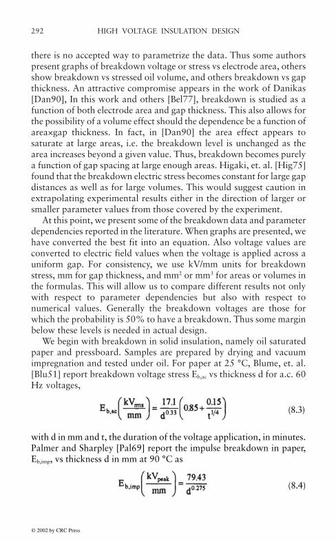
HIGH VOLTAGE INSULATION DESIGN292
there is no accepted way to parametrize the data. Thus some authorspresent graphs of breakdown voltage or stress vs electrode area, othersshow breakdown vs stressed oil volume, and others breakdown vs gapthickness. An attractive compromise appears in the work of Danikas[Dan90], In this work and others [Bel77], breakdown is studied as afunction of both electrode area and gap thickness. This also allows forthe possibility of a volume effect should the dependence be a function ofarea×gap thickness. In fact, in [Dan90] the area effect appears tosaturate at large areas, i.e. the breakdown level is unchanged as thearea increases beyond a given value. Thus, breakdown becomes purelya function of gap spacing at large enough areas. Higaki, et. al. [Hig75]found that the breakdown electric stress becomes constant for large gapdistances as well as for large volumes. This would suggest caution inextrapolating experimental results either in the direction of larger orsmaller parameter values from those covered by the experiment.
At this point, we present some of the breakdown data and parameterdependencies reported in the literature. When graphs are presented, wehave converted the best fit into an equation. Also voltage values areconverted to electric field values when the voltage is applied across auniform gap. For consistency, we use kV/mm units for breakdownstress, mm for gap thickness, and mm2 or mm3 for areas or volumes inthe formulas. This will allow us to compare different results not onlywith respect to parameter dependencies but also with respect tonumerical values. Generally the breakdown voltages are those forwhich the probability is 50% to have a breakdown. Thus some marginbelow these levels is needed in actual design.
We begin with breakdown in solid insulation, namely oil saturatedpaper and pressboard. Samples are prepared by drying and vacuumimpregnation and tested under oil. For paper at 25 °C, Blume, et. al.[Blu51] report breakdown voltage stress Eb,ac vs thickness d for a.c. 60Hz voltages,
(8.3)
with d in mm and t, the duration of the voltage application, in minutes.Palmer and Sharpley [Pal69] report the impulse breakdown in paper,Eb,imp, vs thickness d in mm at 90 °C as
(8.4)
© 2002 by CRC Press

293HIGH VOLTAGE INSULATION DESIGN
In going from 90 °C to 20 °C, the impulse breakdown stress increasesby about 10 % according to [Pal69]. Clark [Cla62] reports for Kraftpaper at room temperature and a.c. test conditions
(8.5)
Results from different investigators are difficult to compare because thethickness buildup is achieved by stacking thin layers of paper. Thestacking processes could differ. Some could use lapping with differentamounts of overlap as well as different thicknesses of the individuallayers. Other possible differences could include the shape and size of theelectrodes. Nevertheless the exponent of the thickness dependence isnearly the same in different studies. Ref. [Cla62] reports an area effectbut it is difficult to quantify. The impulse ratio for paper, corrected fortemperature, based on (8.4) and (8.5) is ~2.7.
For pressboard in oil at 25 °C, Ref. [Blu51] reports
(8.6)
where the frequency f in Hz and time duration t in minutes are takeninto account. The frequency dependence was only tested in the range of25–420 Hz but is expected to hold for even higher frequencies. Forpressboard at room temperature, using 25 mm sphere electrodes, Moser[Mos79] reports
(8.7)
Thus the impulse ratio for pressboard obtained from (8.7) is ~3.0.Ref. [Pal69] reports for pressboard in oil at 90 °C
© 2002 by CRC Press

HIGH VOLTAGE INSULATION DESIGN294
(8.8)
The impulse ratio for pressboard, based on (8.8) is ~3.3. The trend inthe data between Refs. [Mos79] and [Pal69] is in the right directionsince pressboard breakdown strength decreases with increasingtemperature.
Based on the above data, there does not appear to be much differencebetween the breakdown strength of oil soaked paper or pressboardinsulation either under a.c. or impulse test conditions. Even thethickness dependencies are similar. Although Cygan and Laghari[Cyg87] find an area and thickness dependence on the dielectricstrength of polypropylene films, it is not known how applicable this isto paper or pressboard insulation.
For transformer oil at 90 °C, Ref. [Pal69] reports breakdown electricfields which depend on volume Λ in mm3 according to
(8.9)
This would imply an impulse ratio for oil of ~2.5. In contrast to paperinsulation, the breakdown strength of transformer oil increases slightlywith temperature in the range of -5 to 100 °C [Blu51]. Nelson [Nel89]summarizes earlier work on the volume effect for breakdown in oil bymeans of the formula
(8.10)
with Λ in mm3. We should note that the logarithmic dependence onvolume given in (8.9) cannot be valid as volume increases indefinitelysince the breakdown stress would eventually become negative. In (8.10),
© 2002 by CRC Press

295HIGH VOLTAGE INSULATION DESIGN
the breakdown stress becomes unrealistically close to zero as volumeincreases.
Refs. [End57, Web56] present breakdown strength in oil vs electrodearea, A, in the form
(8.11)
The gap spacing in both of these studies was 1.9 mm. Although theimpulse conditions in this study were front of wave, the voltage rampwas kept slow enough in an attempt to approximate full wave conditions.Thus, we can reasonably obtain an impulse ratio from (8.11) of ~2.8.
Ref. [Mos79] gives the a.c. (50 Hz, 1 min) partial dischargeinception electric stress, Epd,ac, for oil as a function of the gap thicknessonly. While not strictly the breakdown strength, partial dischargesmaintained over a long enough time period can lead to breakdown.Separate curves are given for gas saturated or degassed oil and forinsulated and non-insulated electrodes. Fitting the curves, we obtain
with d in mm.Trinh, et. al. [Tri82] analyzed transformer oil for dielectric strength
dependence on both area and volume. They conclude that both areaand volume effects can be present, with the area effect becoming more
(8.12)
© 2002 by CRC Press

HIGH VOLTAGE INSULATION DESIGN296
with A in mm2 and Λ in mm3. They seem to be saying that it is immaterialwhether one describes breakdown in terms of an area or volume effect.However, the consequences of these two approaches are quite different.For areas and volumes in the range of ~103–107 mm2 or mm3, the impulseratio implied by the above formulas is in the range of ~ 2–3. In theseformulas, as is also evident in the work of refs, [Dan90, Hig75], thedielectric strength approaches a constant value as the area or volumebecome very large. This is a reasonable expectation. On the other hand,dielectric strengths approach infinity as areas, volumes, and gap distancesapproach zero in all the above formulas. This is surely inaccurate,although the formulas seem to hold for quite small values of thesequantities.
It can be seen, by putting in typical values for d, A, and Λ as found intransformers in the above formulas, that the dielectric strength of paperor pressboard is approximately twice that of oil. However, the electricstress which occurs in the oil is typically greater than that which occursin the paper or pressboard. For this reason, breakdown generally occursin the oil gaps first. However, once the oil gaps break down, the solidinsulation will see a higher stress so that it could in turn break down.Even if the solid insulation can withstand the higher stress, the
important for ultra clean oil and the volume effect for oil having higherparticle content. Although the data shows much scatter, they presentcurves for oils of different purities. For their technical grade transformeroil, the middle grade of the three analyzed, the following formulas areapproximate fits to their curves.
(8.13)
(8.14)
© 2002 by CRC Press

297HIGH VOLTAGE INSULATION DESIGN
destructive effects of the oil breakdown such as arcing or corona couldeventually puncture the solid insulation. Thus it would seeminappropriate to design a solid-oil insulation system so that the solid byitself could withstand the full voltage applied across the gap as hassometimes been the practice in the past, unless the insulation is all solid.In fact excess solid insulation, because of its higher dielectric constantthan oil, increases the stress in the oil above that of a design moresparing of the solid insulation,
Because of the distance and volume dependence of oil breakdownstrength, it is a common practice to subdivide large oil gaps, as occurfor example between the transformer windings, by means of one ormore thin pressboard cylinders. Thus a gap having a large distance orvolume is reduced to several smaller gaps, each having a higherbreakdown strength. Hence, current practice favors a distance orvolume effect over a pure area effect since gap subdivision would not beof benefit for an area effect. A combination gap-area or gap-volumeeffect would also be consistent with current practice.
The breakdown data referred to above applies to uniform gaps or asreasonably uniform as practical. This situation is rarely achieved indesign so the question arises as to how to apply these results in practice.In volume dependent breakdown, it is suggested that only the oil volumeencompassing electric field values between the maximum and 90 % ofthe maximum be used [Pal69, Wil53]. Thus for concentric cylinderelectrodes, for example, only the volume between the inner cylinder anda cylinder at some fraction of the radial distance to the outer cylinderwould be used in the volume dependent breakdown formulas. For morecomplicated geometries, numerical methods such as finite elements couldbe used to determine this effective volume. For gap distance dependentbreakdown, the suggestion is to subdivide a possible breakdown path intoequal length subdivisions and to calculate the average electric field overeach subdivision. The maximum of these average fields is then comparedwith the breakdown value corresponding to a gap length equal to thesubdivision length. If it exceeds the breakdown value, breakdown alongthe entire path length is assumed to occur. This procedure is repeated forcoarser and coarser subdivisions until a single subdivision consisting orthe entire path is reached. Other possible breakdown paths are thenchosen and the procedure repeated [Nel89, Franc].
Another type of breakdown which can occur in insulation structuresconsisting of solids and liquids or solids and gases is creep breakdown,This occurs along a solid surface in contact with a liquid or gas. Thesepotential breakdown surfaces are nearly unavoidable in insulation
© 2002 by CRC Press

HIGH VOLTAGE INSULATION DESIGN298
design. For example, the oil gaps present in the region betweenwindings are kept uniform by means of sticks placed around thecircumference. The surfaces of these sticks bridge the gap, providing apossible surface breakdown path. Since breakdown along such surfacesgenerally occurs at a lower stress than breakdown in the oil or airthrough the gap itself, surface breakdown is often design limiting. Ref.[Pal69] parametrizes the surface creep breakdown stress alongpressboard surfaces in oil at power frequency, Ecb,ac, in terms of thecreep area, Ac, in mm2 according to
(8.15)
On the other hand, Ref. [Mos79] describes creep breakdown alongpressboard surfaces in oil in terms of the creep distance along the surface,dc, in mm according to
(8.16)
For non-uniform field situations, the same procedure of path subdivisionand comparison with the creep breakdown strength calculated by (8.16)is followed as was described earlier for gap breakdown.
8.3 INSULATION COORDINATION
Insulation coordination concerns matching the insulation design to theprotective devices used to limit the voltages applied to the terminals ofa transformer by lightning strikes or switching surges and possibly otherpotentially hazardous events. Since the insulation must withstand thenormal operating voltages which are present continuously as well aslightning or switching events which are of short duration, how breakdowndepends on the time duration of the applied voltage is of major importancein insulation coordination. We have seen previously that the impulseratio is ~2–3 for oil filled transformer insulation. This means that thebreakdown strength of a short duration impulse voltage lasting ~5–10µs is much higher than the breakdown strength of a long duration (~1min) a.c. voltage. It appears that, in general, breakdown voltages orstresses decrease with the time duration of the voltage application fortransformer insulation. The exact form of this breakdown vs timedependence is still somewhat uncertain, probably because of variations
© 2002 by CRC Press
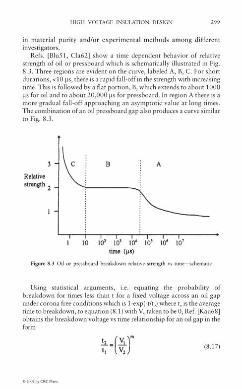
299HIGH VOLTAGE INSULATION DESIGN
in material purity and/or experimental methods among differentinvestigators.
Refs. [Blu51, Cla62] show a time dependent behavior of relativestrength of oil or pressboard which is schematically illustrated in Fig.8.3. Three regions are evident on the curve, labeled A, B, C. For shortdurations, <10 µs, there is a rapid fall-off in the strength with increasingtime. This is followed by a flat portion, B, which extends to about 1000µs for oil and to about 20,000 µs for pressboard. In region A there is amore gradual fall-off approaching an asymptotic value at long times.The combination of an oil pressboard gap also produces a curve similarto Fig. 8.3.
Using statistical arguments, i.e. equating the probability ofbreakdown for times less than t for a fixed voltage across an oil gapunder corona free conditions which is 1-exp(-t/to) where to is the averagetime to breakdown, to equation (8.1) with Vo taken to be 0, Ref. [Kau68]obtains the breakdown voltage vs time relationship for an oil gap in theform
(8.17)
Figure 8.3 Oil or pressboard breakdown relative strength vs time—schematic
© 2002 by CRC Press
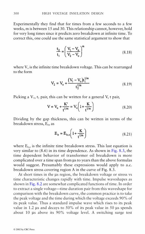
HIGH VOLTAGE INSULATION DESIGN300
Experimentally they find that for times from a few seconds to a fewweeks, m is between 15 and 30. This relationship cannot, however, holdfor very long times since it predicts zero breakdown at infinite time. Tocorrect this, one could use the same statistical argument to show that
(8.18)
where Vo is the infinite time breakdown voltage. This can be rearrangedto the form
(8.19)
Picking a V1, t1 pair, this can be written for a general V, t pair,
(8.20)
Dividing by the gap thickness, this can be written in terms of thebreakdown stress, Eb, as
(8.21)
where Eb,o is the infinite time breakdown stress. This last equation isvery similar to (8.6) in its time dependence. As shown in Fig. 8.3, thetime dependent behavior of transformer oil breakdown is morecomplicated over a time span from µs to years than the above formulaswould suggest. Presumably these expressions would apply to a.c.breakdown stress covering region A in the curve of Fig. 8.3.
At short times in the µs region, the breakdown voltage or stress vstime characteristic changes rapidly with time. Impulse waveshapes asshown in Fig. 8.2 are somewhat complicated functions of time. In orderto extract a single voltage—time duration pair from this waveshape forcomparison with the breakdown curve, the common practice is to takethe peak voltage and the time during which the voltage exceeds 90% ofits peak value. Thus a standard impulse wave which rises to its peakvalue in 1.2 µs and decays to 50% of its peak value in 50 µs spendsabout 10 µs above its 90% voltage level. A switching surge test
© 2002 by CRC Press

301HIGH VOLTAGE INSULATION DESIGN
waveshape is similar to that of Fig. 8.2 but the rise time to peak value is~100 µs and the fall time to the 50 % level is ~500 µs. The time spentabove the 90% of peak voltage level is ~200 µs. Therefore we wouldexpect breakdown to occur on a switching surge test at a lower voltagethan for a full wave impulse test.
Two other types of impulse test are the chopped wave test and frontof wave test, although the latter is considered unnecessary in view ofmodern methods of protection. A standard chopped wave, as shown inFig. 8.4, rises to its peak in ~1.2 µs and abruptly falls to zero with aslight undershoot at the chop time of ~3 µs. It is above its 90% of peakvoltage for ~3 µs. The front of wave is chopped on the rising part of thewave and has a duration above 90 % of its maximum value of ~0.5 µs.The generally accepted breakdown levels corresponding to thesedifferent times, normalized to the full wave breakdown level, are givenin Table 8.1.
Figure 8.4 Chopped wave impulse waveshape
© 2002 by CRC Press

HIGH VOLTAGE INSULATION DESIGN302
We have included in Table 8.1 two other points, the 1 minute a.c. testpoint and the essentially infinite time nominal voltage point. For the 1min test point, we have used an impulse ratio of 2.8. Thus thenormalized breakdown peak voltage level is 1/2.8×√2=0.5 and theduration above 90% of the peak voltage is 0.287×60 sec=17.2 sec. Wehave taken the nominal system voltage to be half the 1 min test voltage.Other values for these could have been chosen with equal justification.For instance, an impulse ratio of 2.4 is commonly assumed in settingtest values and the nominal voltage can be a factor of 2.5–3.0 below the1 min test level. Note that the nominal system voltage used here is fromterminal to ground.
We can produce a reasonable fit to the above tabular values with anequation of the form (8.20). Letting Vb,rel be the breakdown levelsrelative to the full wave level, we obtain
(8.22)
with t in µs. Table 8.1 is based on practical experience in testingtransformers. The numbers can only be regarded as approximate anddifferent choices are often made within a reasonable range about thevalues shown. This would influence the fit given in (8.22) or possiblyrequire a different parametrization. This parametrization may have nofundamental significance since it does not apply to any carefullycontrolled experiment. However its form, which agrees with the morefundamentally based equation (8.20), is noteworthy.
In practical applications, a table like Table 8.1 provides a way oflinking the various test voltages to the full wave impulse voltage whichis also called the basic impulse level (BIL). Since the required impulsetest levels are usually linked to the lightning or surge arrester protectionlevel whereas the a.c. test levels or nominal voltage level are not, they
Table 8.1 Breakdown voltages normalized to the full wave impulse level
© 2002 by CRC Press

303HIGH VOLTAGE INSULATION DESIGN
can be specified independently. For example, a 500 kVrms line to linetransformer (=288 kVrms line to ground=408.2 kVpeak line to ground)would correspond to a full wave impulse level of 1633 kV according toTable 8.1. However, the user may have sufficient protection that only a1300 kV impulse test is required. Nevertheless, the insulation wouldhave to be designed to withstand a full wave 1633 kV impulse test, eventhough not performed, since that level of protection is required toguarantee satisfactory operation at the nominal 500 kVrms line to linevoltage. As another example, one may have breakdown stress vsdistance, area, or volume curves for 1 min a.c. test conditions. In orderto compare these to the stress levels generated in a simulated impulsetest calculation, one needs to know the relative breakdown level factorsgiven in Table 8.1.
8.4 CONTINUUM MODEL OF WINDING USED TO OBTAINTHE IMPULSE VOLTAGE DISTRIBUTION
For very short times after the application of a voltage to a windingterminal, the voltage distribution along the winding is governed primarilyby capacitive coupling. This is because the winding inductance limitsthe flow of current initially. In this approximation, a winding can bemodeled by the capacitive ladder diagram shown in Fig. 8.5a. Althoughdiscrete capacitances are shown, this is meant to be a continuum model.The calculation outlined here is similar to that given in Chapter 7.Some of the steps are repeated in order to more easily compare theresults with the travelling wave theory. Thus, as shown in Fig. 8.5b, theseries capacitors, cs, are separated by a distance ∆x, where ∆x willeventually approach zero. The series capacitors are determined by thewinding structure, including the number of disks, their spacing, and thenumber of turns/disk. The ground capacitors, cg, are determined by thedistance to neighboring windings or to the tank walls or core. These areall assumed to be at ground potential relative to the impulsed winding,which should be true initially.
© 2002 by CRC Press
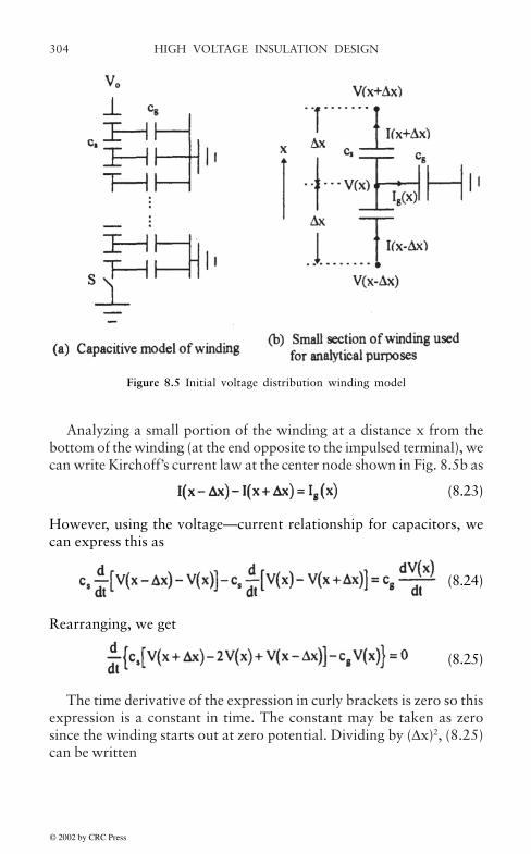
HIGH VOLTAGE INSULATION DESIGN304
Analyzing a small portion of the winding at a distance x from thebottom of the winding (at the end opposite to the impulsed terminal), wecan write Kirchoff’s current law at the center node shown in Fig. 8.5b as
(8.23)
However, using the voltage—current relationship for capacitors, wecan express this as
(8.24)
Rearranging, we get
(8.25)
The time derivative of the expression in curly brackets is zero so thisexpression is a constant in time. The constant may be taken as zerosince the winding starts out at zero potential. Dividing by (∆x)2, (8.25)can be written
Figure 8.5 Initial voltage distribution winding model
© 2002 by CRC Press
305HIGH VOLTAGE INSULATION DESIGN
(8.26)
The term on the left hand side can be recognized as the second orderdifference operator which approaches the second derivative as ∆x→0. IfL is the length of the winding, there are N=L/∆x series capacitors, cs,and ground capacitors, cg. In terms of the total series and groundcapacitances, Cs and Cg, we have
(8.27)
Substituting into (8.26) and letting ∆x→0, we obtain
(8.28)
where the distribution constant α has been defined as
(8.29)
If the bottom of the winding is grounded (switch S closed in Fig. 8.5a)and a voltage Vo is applied at the line end, the solution to (8.28) is
(8.30)
When the switch S is open so that the bottom of the winding is floatingwhen the voltage Vo is applied to the top of the winding, the solution to(8.28) is
(8.31)
© 2002 by CRC Press

HIGH VOLTAGE INSULATION DESIGN306
Equation (8.30) is plotted in Fig. 8.6 for several values of α. As canbe seen, the slope of the curve becomes very steep at the line end asincreases. This implies that the disk-disk voltage, ∆Vd, increases withincreasing α since this is given approximately as
(8.32)
where w is the disk-disk spacing, assumed small compared with L.This has its maximum value at the line end where x=L,
(8.33)
For the ungrounded winding, the maximum stress again occurs at theline end and, using (8.31), is
(8.34)
which is somewhat less than (8.33) since |tanhα| ≤ 1. If the voltagedistribution is uniform or α small, ∆Vd,line=Vo(w/L) for the grounded endcase.
© 2002 by CRC Press

307HIGH VOLTAGE INSULATION DESIGN
Since the disk-disk stress increases with α and by implication theturn-turn stress also, (8.29) suggests that to reduce this we need toincrease Cs or decrease Cg or both. This has led to winding schemes suchas interleaving which can dramatically increase the series capacitance.Interleaving schemes can be quite complicated and need not be appliedto the whole winding. In addition, the scheme may vary within a givenwinding. A multi-start winding is an example of a simple interleavingscheme for increasing the series capacitance of a tap winding. Anothermethod of increasing the series capacitance is by means of wound-in-shields which can be applied to a section of the winding near the lineend where they are most needed. Decreasing Cg is not as promisingsince this would involve, at least in a simple approach, increasing thewinding to winding or winding to tank distance for an outer winding ordecreasing the winding height for a given radius. Such changes couldconflict with impedance or cooling requirements,
An improvement over the static capacitance model is a model whichincludes the winding inductance in an approximate way. This is thetraveling wave theory as developed by Rudenberg [Rud68, Rud40].This is also a continuum model with the circuit parameters defined on aper unit length basis. Thus, using primes to indicate per unit length, the
Figure 8.6 Initial voltage distribution along a winding for various values of α.
© 2002 by CRC Press

HIGH VOLTAGE INSULATION DESIGN308
capacitances per unit length become, in terms of our previous notationwith w the disk-disk distance,
(8.35)
and a new variable ' which is the inductance/unit length. Thus thetotal series and ground capacitances, expressed in terms of the primedquantities are, using (8.27),
(8.36)
since w=∆x in this context. Hence α can be written,
(8.37)
The use of an inductance per unit length can only be regarded asapproximate since it ignores the mutual inductance between the differentsections of the winding. This approximation can be justified to someextent mathematically and by comparison with experiment.
Without going into all the details, the resulting differential equationcan be solved by a superposition of traveling waves of the form
(8.38)
with v the wave velocity and ω its angular frequency related by
(8.39)
At low frequencies, ω→0,
(8.40)
At higher frequencies the wave velocity eventually becomes zero at thecritical frequency, ωo, given by
© 2002 by CRC Press

309HIGH VOLTAGE INSULATION DESIGN
(8.41)
Thus input waves or Fourier components of input waves of this frequencyor higher cannot travel into the winding. However, at higher frequencies,v becomes imaginary and the solution (8.38) takes the form
V=Voejωt-βx (8.42)
with β given by
(8.43)
Thus the higher frequencies exponentially decay with distance into thewinding, (Here x measures the distance from the line end.) At high ω,this becomes asymptotically
(8.44)
where the last equality follows from (8.37).Rudenberg [Rud68, Rud40] considers the special case of a step
function input to the line end of the winding as shown in Fig. 8.7, At theline terminal where x=0, this wave can be written as a Fourier integral,
(8.45)
where Vo is its amplitude. As the integral shows, the frequency componentamplitudes decrease with increasing frequency. However, as we haveseen previously, only frequency components below the critical frequencyωo can travel into the winding. Higher frequency components give riseto an exponentially decaying standing wave. Thus, the wave penetratinginto the winding has the form
© 2002 by CRC Press

HIGH VOLTAGE INSULATION DESIGN310
(8.46)
Because of the truncation of the integral, V' no longer has a step functionshape but penetrates into the winding with the shape shown in Fig. 8.8.Thus the steep front has been flattened.
Figure 8.7 Step function voltage wave impinging on winding terminal
The flattened wave can be approximated by the dotted lines shownin Fig. 8.8. This consists of a sloped straight line front connecting thehorizontal straight line asymptotic values. The time duration of this
Figure 8.8 Flattened wave which enters the winding starting from the rectangularwave shown in Fig. 8.7
© 2002 by CRC Press
311HIGH VOLTAGE INSULATION DESIGN
front, τ, is determined by the properties of the integral in (8.46) and isgiven by
(8.47)
using (8.41). For the lower frequencies comprising this pulse, we canapproximate their velocity by vo as given in (8.40). Thus the length ofthe sloped portion of the pulse in Fig. 8.8. H, is given approximately by
(8.48)
Using (8.44), this can be written
(8.49)
This sloped front causes a voltage difference across the winding diskswhich is given by
(8.50)
For the decaying exponential part of the pulse, β can be taken to agood approximation as β∞. Its amplitude, according to Rudenberg, isVo/2. It is therefore given by
(8.51)
Thus the disk-disk voltage drop due to this voltage is given in magnitudeby
(8.52)
Combining (8.50) and (8.52), the overall disk-disk voltage drop is givenby
© 2002 by CRC Press
HIGH VOLTAGE INSULATION DESIGN312
(8.53)
At x=0, this becomes
(8.54)
For α>3 which is somewhat typical, tanhα≈1, so that comparing thislast equation with its counterpart for the purely capacitive case, (8.33)or (8.34), we see that the voltage drop in the traveling wave case is~18%less than for the capacitive case. However, because of the slight overand under shoots of the actual wave as shown in Fig. 8.8, this differenceis not that great.
Norris [Nor48] has proposed an improved version of (8.53) whichhas the form
(8.55)
where Kg=Ho/Hx, where Hx is the length of the sloped front of the travelingwave a distance x into the winding. The wave spreads out because thedifferent frequency components travel with different velocities and thusKg≤1. Kg can be found as a solution of the equation [Rud68, Rud40]
(8.56)
This reduces to a quartic equation which can be solved analytically. Atx=0 and for α>3, (8.55) is equal to disk-disk voltage drop in the capacitivecase as can bee seen by comparison with (8.33). Norris has also suggestedcorrections for incoming waves having finite rise and fall times andgives procedures for handling non-uniform windings.
© 2002 by CRC Press

313HIGH VOLTAGE INSULATION DESIGN
8.5 LUMPED PARAMETER MODEL FOR TRANSIENT VOLTAGEDISTRIBUTION
In this section, we develop a circuit model of the transformer whichincludes capacitive, inductive, and resistive elements. The inductiveelements include mutual inductances between elements in the samewinding and in different windings and the effects of the iron core. Thecoils can be subdivided into as fine or coarse a manner as is consistentwith the desired accuracy. Moreover, the subdivisions can be unequalso that accuracy in certain parts of the coil can be increased relative tothat in other parts. The approach taken is similar to that of Miki, et. al.[Mik78] except that it includes winding resistance and the effects of theiron core. Also the differential equations describing the circuit areorganized in such a way that circuit symmetries can be exploited andother circuit elements such as non-linear varistors may be included.
8.5.1 Circuit Description
A transformer is approximated as a collection of lumped circuit elementsas shown in Fig. 8.9. Although not shown, mutual inductances betweenall the inductors are assumed to be present. The subdivisions maycorrespond to distinctly different sections of the coil, having differentinsulation thicknesses for example, or may simply be present for increasedaccuracy. The core and tank are assumed to be at ground potential. Thepresence of the tank only affects the capacitance to ground of the outercoil but not the inductance calculation. Other elements such as groundingresistors, capacitors, inductors, or non-linear elements may be added.Terminals or nodes may be interconnected, shorted to ground, orconnected to ground via a resistor, reactor, capacitor, or varistor.
In order to analyze the circuit of Fig. 8.9, we isolate a representativeportion as shown in Fig. 8.10. We adopt a node numbering schemestarting from the bottom of the innermost coil and proceeding upward.Then continue from the bottom of the next coil, etc. Similarly, a sectionor subdivision numbering scheme is adopted, starting from the bottomof the innermost coil, proceeding upward, etc. These numberingschemes are related. In the figure, we have simply labeled the nodeswith i (p’s and q’s for adjacent nodes) and the sections with j. Our circuitunknown are the nodal voltages Vi and section currents Ij directedupward as shown.
© 2002 by CRC Press

HIGH VOLTAGE INSULATION DESIGN314
Figure 8.9 Circuit model of transformer. The number of coils and subdivisions withina coil are arbitrary.
© 2002 by CRC Press

315HIGH VOLTAGE INSULATION DESIGN
Considering the voltage drop from node i-1 to node i, we can write
(8.57)
where Mjk is the mutual inductance between sections j and k. Defining asection current vector I, a nodal voltage vector V, an inductance matrixM, where Mjj=Lj, and a diagonal resistance matrix R, we can compressthe above formula as
(8.58)
where B is a rectangular matrix whose rows correspond to sections andcolumns to nodes such that Bji-1=1 and Bji=-1, where nodes i-1 and ibracket section j. The inductance matrix M is a symmetric positive
Figure 8.10 Representative portion of Fig. 8.9.
© 2002 by CRC Press

HIGH VOLTAGE INSULATION DESIGN316
definite matrix. Equation (8.58) holds independently of how the terminalsare interconnected or what additional circuit elements are present.
Applying Kirchoff’s current law to node i, we obtain
(8.59)
where the p-sum is over all nodes connected to node i via shuntcapacitances Kip. Cj is set to zero when node i is at the bottom of the coiland Cj+1=0 when node i is at the top of the coil, although a small valuefor capacitive coupling to the yokes could be used. dVp/dt=0 when nodep is at ground potential such as for the core or tank. Defining acapacitance matrix C, (8.59) can be rewritten as
(8.60)
where A is a rectangular matrix whose rows correspond to nodes andcolumns to sections and where Aij=1 and Aij+1=-1, with sections j and j+1on either side of node i. One of these terms is 0 when i is at the end of acoil.
When a nodal voltage Vi is specified, for example at the impulsedterminal, as Vi=Vs, equation (8.59) is replaced by
(8.61)
If Vs=0 as for a grounded terminal, then (8.61) becomes dVi/dt=0. Whennode i is shorted to ground via a resistor Rs, a term Vi/Rs is added to theleft hand side of (8.59). If node i is grounded by means of a capacitor Cs,a term CsdVi/dt is added to the left hand side of (8.59). For a shortinginductor Ls uncoupled from all the other inductors, a term + Vidt/Ls isadded to the left hand side of (8.59). Other situations such as a resistoror varistor joining two nodes can be easily accommodated.
When several nodes are joined together, say nodes i, r, s,…, theirKirchoff’s current law equations are simply added. The resultingequation replaces the node i equation. Then the node r, s,…equationsare replaced by
© 2002 by CRC Press

317HIGH VOLTAGE INSULATION DESIGN
(8.62)
The net result of all these circuit modifications is that the capacitancematrix in (8.60) may be altered and the right hand side may acquireadditional terms, e.g. terms involving V for a resistor, +∫Vdt for aninductor, and the impulsed voltage Vs. Thus (8.60) is replaced by
(8.63)
where C' is the new capacitance matrix and f depends on the addedelements. The above procedure lends itself to straightforward computerimplementation.
Equations (8.58) and (8.63) can now be solve simultaneously bymeans of for example a Runge-Kutta algorithm starting from a giveninitial state. Linear equations must be solved at each time step todetermine dI/dt and dV/dt. Since M is a symmetric positive definitematrix, the Cholesky algorithm may be used to solve (8.58) while (8.63)may be solved by Gaussian elimination. LLT or LU factorization is firstperformed on the respective matrices and the factors are usedsubsequently to solve the linear equations at each time step, savingmuch computation time.
8.5.2 Mutual and Self Inductance Calculations
The transformer core and coil geometry including the iron yokes isassumed to have cylindrical symmetry. The iron is assumed to beinfinitely permeable. A typical coil section is shown in Fig. 8.11. It isassumed to be rectangular in cross-section and carry a uniform currentdensity J, azimuthally directed. The yokes extend outward to infinityand we ignore the tank walls. This geometry corresponds to that used inthe Rabins’ inductance and mutual inductance calculations of Chapter5. However, we will use a slightly different method to obtain the selfand mutual inductances. For two coil sections, labeled p and q, wherep=q indicates a self inductance calculation, the mutual (or self) inductanceis given by
(8.64)
© 2002 by CRC Press

HIGH VOLTAGE INSULATION DESIGN318
Using the vector potential solution given in Chapter 5 but labelingthe inner and outer coil section radii by rip, rop, riq, roq for sections p andq respectively, we find for coil sections on different radially displacedcoils.
where Ap is the vector potential generated by section p, Ip and Iq the totalcurrents in the two coil sections, and the volume integral is only overthe coil section q and not the entire window height L since this is whereall the current would be located if we used an infinite number of termsin the Fourier expansion of the current density. This produces the sameresult as before but we use slightly different notation here.
Figure 8.11 Geometry of iron core, yokes, and coil section.
(8.65)
© 2002 by CRC Press

319HIGH VOLTAGE INSULATION DESIGN
The coefficients Gn,p, En,p, Fn,p are as defined in Chapter 5. The modifiedBessel and Struve function integrals can be evaluated by the numericaltechniques given there.
8.5.3 Capacitance Calculations
The series capacitances must take into account the type of coil, whetherhelix, disk, multi-start, or other. Series and shunt capacitancesincorporate details of the paper and pressboard insulation, the placementof key spacers and sticks, and the oil duct geometry. Except when wound-in-shields are present, the formula developed by Stein as discussed inChapter 7 is used for the series disk capacitances. This formula wasfound to produce the best results in the work reported by Miki et. al.[Mik78]. Simple standard formulas are used for helical and multi-startwindings as well as for shunt capacitances as discussed in Chapter 7.Basically a shunt capacitance per unit length is calculated, assumingthe coils are infinitely long, and this is multiplied by the length of thesection to get the section to section or section to ground shunt capacitances.
The series capacitance for a section containing several disks or turnsin the case of a helical winding is obtained by adding the single diskcapacitances in series, i.e. dividing the single disk capacitance by thenumber of disks in the section. Since the subdivisions need not containan integral number of disks, fractional disks are allowed in thiscalculation. Other subdivision schemes could be adopted which restrictthe sections to contain an integral number of disks. When wound-in-shields are present, only an integral number of disk pairs are allowed inthe subdivision. The finer the subdivisions or the greater their number,the greater the expected accuracy. However, too fine a subdivision, sayless than the height of a disk, could be counterproductive. Finesubdivisions can also lead to convergence problems for the Fouriersums in the mutual inductance calculation.
where m=nπ/L as before. For coil sections on the same coil, we obtain
(8.66)
© 2002 by CRC Press

HIGH VOLTAGE INSULATION DESIGN320
8.5.4 Impulse Voltage Calculations and Experimental Comparisons
The standard impulse voltage waveform can be mathematicallyrepresented as
(8.67)
where κ1, κ2, and Vo are adjusted so that Vs rises to its maximum valuein 1.2 µs and decays to half its value in 50 µs. It is desirable to have ananalytic formula which is smoothly differentiable such as (8.67) sincethe derivative is used in the solution process. Other waveforms such asa chopped wave may also be used. Procedures may be developed forextracting the parameters used in (8.67) from the desired rise and falltimes and peak voltage. In our experimental RSO tests discussed below,the actual rise and fall times were 3 and 44 µs respectively and theparameters in (8.67) were adjusted accordingly.
We tested a 45 MVA autotransformer having 4 windings as shown inFig. 8.12. The high voltage (HV or series) winding consists of 2 coils inparallel with two ends joined at the center where the impulse is applied.The other two ends are joined at the autopoint with the low voltage (LVor common) and tap windings. The HV and LV windings are diskwindings. The tap winding is a multi-start winding and is grounded forthe impulse test. The tertiary voltage winding (TV) is a helical windingand is grounded at both ends for the impulse test. These windingsrepresent one phase of a three phase transformer but are essentiallyisolated from each other for the impulse test.
Both the HV and TV windings contain tapped sections along theirlengths. The tap turns are out on the HV winding and in on the TVwinding during the impulse test. In the calculations a direct short isplaced across the tapped out sections. In the vicinity of these tap
© 2002 by CRC Press
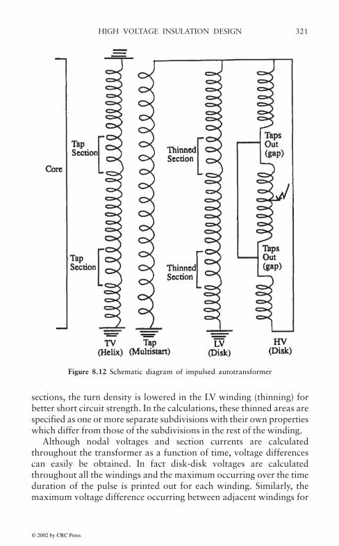
321HIGH VOLTAGE INSULATION DESIGN
sections, the turn density is lowered in the LV winding (thinning) forbetter short circuit strength. In the calculations, these thinned areas arespecified as one or more separate subdivisions with their own propertieswhich differ from those of the subdivisions in the rest of the winding.
Although nodal voltages and section currents are calculatedthroughout the transformer as a function of time, voltage differencescan easily be obtained. In fact disk-disk voltages are calculatedthroughout all the windings and the maximum occurring over the timeduration of the pulse is printed out for each winding. Similarly, themaximum voltage difference occurring between adjacent windings for
Figure 8.12 Schematic diagram of impulsed autotransformer
© 2002 by CRC Press

HIGH VOLTAGE INSULATION DESIGN322
the duration of the pulse is also printed out. Secondary quantities suchas maximum electric fields in the oil can likewise be obtained.
Experimentally only voltages along the high voltage coil and at thetap positions on the tertiary winding were easily accessible in the testsconducted. In a recurrent surge oscillograph (RSO) test, a repetitiveseries of pulses having the shape described by (8.67) are applied to, inour case, the HV terminal This repetitive input results in persistentoscilloscope displays of the output voltages for easy recording. Thepeak applied voltage is usually low, typically several hundred volts.This test simulates an impulse test done at much higher voltages to theextent that the system is linear. This is likely to be a good assumptionprovided the core doesn’t saturate and provided non-linear circuitelements such as varistors do not come into play. In our RSO test, thetransformer was outside the tank. Thus the dielectric constant of air wasused in the capacitance formulas. In addition the tank distance, whichaffects the ground capacitance of the outer coil, was taken as very large.
For the tests conducted here, the computer outputs of interest werethe voltages to ground at the experimentally measured points. Wepresent a sufficient number of these in the following figures to indicatethe level of agreement between calculation and experiment. We choseto normalize the input to 100 at the peak of the impulse waveform. Theunits can therefore be interpreted as a percent of the BIL.
It quickly became apparent in comparing the simulations withexperiment that the section resistances which were obtained from thewire geometry and the d.c. or power frequency resistivity was notadequate to account for the damping observed in the output waveforms.In fact, we found it necessary to increase this resistivity by a factor ofabout 3000 to account for the damping. Such a factor is notunreasonable in view of the fact that the currents induced by theimpulse waveform contain high frequency components which inducemuch higher losses than occur at power frequency. A factor of thismagnitude was estimated for the experiment involving wound-in-shields in Chapter 7. A better approach which we subsequently adoptedis to Fourier analyze the current waveforms and calculate the effectiveresistivity using the formula given in Chapter 7. This involves runningthe calculation at least twice, once to obtain the waveforms using anassumed resistivity. Fourier analyzing the waveforms to obtain a betterestimate of the effective resistivity, and then re-running the calculationwith the recalculated resistivity.
Each of the two HV coils had 52 disks having 12 radial turns each.The impulse was applied to the center of the leg where the two coils are
© 2002 by CRC Press

323HIGH VOLTAGE INSULATION DESIGN
joined. Output voltages are recorded relative to this center point. Fig.8.13 shows the experimental and calculated voltage waveform 4 disksbelow the impulsed terminal. The impulse voltage is also shown forcomparison. Fig. 8.14 shows the voltage 12 disks below the impulsedterminal. There is good agreement in the major oscillations but somedifferences in the lower amplitude higher frequency oscillations. Fig. 8.15shows the experimental and theoretical voltages at the tap position whichis about 30 disks below the impulsed terminal. Fig. 8.16 shows thevoltage transferred to the upper tap position on the TV winding. There isgood agreement between theory and experiment in overall magnitudeand major oscillations but the higher frequency ripple is not as wellpredicted. Fig. 8.17 indicates another way to present the calculations.This shows the voltage as a function of relative coil position along the topHV winding at various instants of time. Note the flat portion of the curvesat a relative position of ~0.75 which corresponds to the tap section withthe taps out. Note also that the high capacitance of the multi-start tapwinding effectively grounds the autopoint. Maximum disk-disk voltagescould be obtained by examining such curves although this is more easilydone by programming.
Figure 8.13 Experimental and calculated voltage to ground 4 disks below the HVimpulsed terminal. The impulse voltage is also shown.
© 2002 by CRC Press

HIGH VOLTAGE INSULATION DESIGN324
Figure 8.14 Experimental and calculated voltage to ground 12 disks below the HVimpulsed terminal
Figure 8.15 Experimental and theoretical voltages to ground at the tap position onthe HV winding, about 30 disks below the impulsed terminal
© 2002 by CRC Press
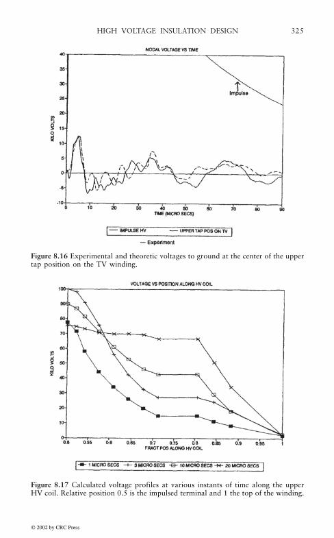
325HIGH VOLTAGE INSULATION DESIGN
Figure 8.16 Experimental and theoretic voltages to ground at the center of the uppertap position on the TV winding.
Figure 8.17 Calculated voltage profiles at various instants of time along the upperHV coil. Relative position 0.5 is the impulsed terminal and 1 the top of the winding.
© 2002 by CRC Press
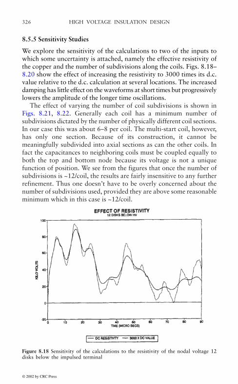
HIGH VOLTAGE INSULATION DESIGN326
8.5.5 Sensitivity Studies
We explore the sensitivity of the calculations to two of the inputs towhich some uncertainty is attached, namely the effective resistivity ofthe copper and the number of subdivisions along the coils. Figs. 8.18–8.20 show the effect of increasing the resistivity to 3000 times its d.c.value relative to the d.c. calculation at several locations. The increaseddamping has little effect on the waveforms at short times but progressivelylowers the amplitude of the longer time oscillations.
The effect of varying the number of coil subdivisions is shown inFigs. 8.21, 8.22. Generally each coil has a minimum number ofsubdivisions dictated by the number of physically different coil sections.In our case this was about 6–8 per coil. The multi-start coil, however,has only one section. Because of its construction, it cannot bemeaningfully subdivided into axial sections as can the other coils. Infact the capacitances to neighboring coils must be coupled equally toboth the top and bottom node because its voltage is not a uniquefunction of position. We see from the figures that once the number ofsubdivisions is ~12/coil, the results are fairly insensitive to any furtherrefinement. Thus one doesn’t have to be overly concerned about thenumber of subdivisions used, provided they are above some reasonableminimum which in this case is ~12/coil.
Figure 8.18 Sensitivity of the calculations to the resistivity of the nodal voltage 12disks below the impulsed terminal
© 2002 by CRC Press
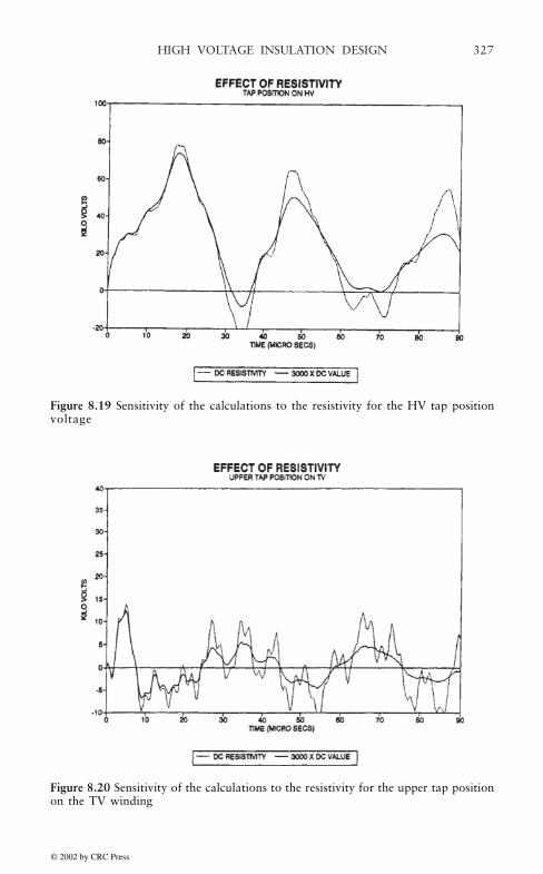
327HIGH VOLTAGE INSULATION DESIGN
Figure 8.19 Sensitivity of the calculations to the resistivity for the HV tap positionvoltage
Figure 8.20 Sensitivity of the calculations to the resistivity for the upper tap positionon the TV winding
© 2002 by CRC Press

HIGH VOLTAGE INSULATION DESIGN328
Figure 8.21 Effect of the number of coil subdivisions on the voltage for a point 12disks below the impulsed terminal
Figure 8.22 Effect of the number of coil subdivisions on the voltage at the tapposition on the HV winding
© 2002 by CRC Press

329
9. ELECTRIC FIELD CALCULATIONS
Summary The electric field is calculated for some idealized insulationstructures which can often be useful approximations to actual insulationsystems. This can provide insight into the parameter dependence of suchfields and can suggest ways of reducing such fields if necessary. The electricfields in the oil gaps between pairs of disks in a transformer winding arestrongest at the corners. These corner fields therefore determine the gapspacing and paper insulation required to avoid breakdown. We determinethese fields by means of a conformal mapping technique for a 2-D geometryconsisting of 2 conductors at different potentials separated by a gap (disk—disk spacing). Both conductors are separated by another gap from a groundplane. This latter gap could be a winding—winding gap or a winding—core or tank gap. The analytic solution does not include the effect of thepaper insulation. This leads to an enhancement of the field in the oil overthe situation without insulation. A method is proposed to account for theinsulation based on a comparison with a finite element solution. Finiteelement solution methods are discussed for complex geometries.
9.1 SIMPLE GEOMETRIES
It is often possible to obtain a good estimation of the electric field in acertain region of a transformer by idealizing the geometry to such anextent that the field can be calculated analytically. This has the advantageof exhibiting the field as a function of several parameters so that theeffect of changing these and how this affects the field can be appreciated.Such insight is often worth the price of the slight inaccuracy which mayexist in the numerical value of the field.
As a first example, we consider a layered insulation structure havinga planar geometry as shown in Fig. 9.1. This could represent the majorinsulation structure between two cylindrical windings having largeradii. We are further approximating the disk structure as a smoothsurface so that the resulting field calculation would be representative ofthe field away from the corner of the disks. We treat this corner field inthe next section.
© 2002 by CRC Press
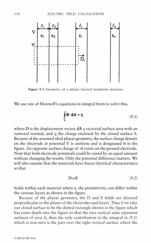
ELECTRIC FIELD CALCULATIONS330
We use one of Maxwell’s equations in integral form to solve this,
(9.1)
where D is the displacement vector, dA a vectorial surface area with anoutward normal, and q the charge enclosed by the closed surface S.Because of the assumed ideal planar geometry, the surface charge densityon the electrode at potential V is uniform and is designated σ in thefigure. An opposite surface charge of -σ exists on the ground electrode.Note that both electrode potentials could be raised by an equal amountwithout changing the results. Only the potential difference matters. Wewill also assume that the materials have linear electrical characteristicsso that
D=εE (9.2)
holds within each material where ε, the permittivity, can differ withinthe various layers as shown in the figure.
Because of the planar geometry, the D and E fields are directedperpendicular to the planes of the electrodes and layers. Thus if we takeour closed surface to be the dotted rectangle shown in the figure whichhas some depth into the figure so that the two vertical sides representsurfaces of area A, then the only contribution to the integral in (9.1)which is non-zero is the part over the right vertical surface where the
Figure 9.1 Geometry of a planar layered insulation structure
© 2002 by CRC Press

ELECTRIC FIELD CALCULATIONS 331
displacement vector has the uniform value labelled Di in the figure.Thus, for this closed surface (9.1) becomes
(9.3)
Using (9.2) applied to layer i, (9.3) becomes
(9.4)
In terms of the potential V, we can write by definition
(9.5)
where the line integral starts at the 0 potential electrode and ends on theV potential electrode. In terms of the E fields in the different materialsand their thicknesses i, (9.5) becomes
(9.6)
Using (9.4), this can be written
(9.7)
Solving for σ and substituting into (9.4), we get
(9.8)
Letting be the total distance between the electrodes so that =1+2
+…and defining the fractional lengths, fi=i/, (9.8) can be expressed as
© 2002 by CRC Press
ELECTRIC FIELD CALCULATIONS332
(9.9)
where Eo is the electric field between the electrodes if there was only onelayer of uniform material between them.
Let’s apply these results to an oil-pressboard insulation system. Evenif there are many layers of pressboard used to subdivide the oil gap,only the total fractional thickness, fpress, matters in the calculation.Similarly, the subdivided oil gap's total fractional thickness, foil=1-fpress,is all that is needed to perform the calculation, For this situation, (9.9)becomes
(9.10)
Since the relative permittivities of pressboard and oil are , the electric field in the oil is about twice as high as the electric
field in the pressboard for a given oil-pressboard combination. Thusthe oil’s electric field is usually the most important to know for purposesof breakdown estimation. We plot Eoil/Eo vs fpress in Fig. 9.2. We seefrom the figure that for a given oil gap, the lowest field results whenthere is no pressboard. As more pressboard displaces the oil, the fieldin the oil increases, approaching a value of twice its all oil value whenthe gap is nearly filled with pressboard.
© 2002 by CRC Press

ELECTRIC FIELD CALCULATIONS 333
A somewhat better estimate can be made of the electric field in themajor insulation structure between two coils if we considerapproximating the geometry as an ideal cylindrical geometry. Thisgeometry is also useful for approximating the field around a long cableof circular cross section. We consider the general case of a multi-layerconcentric cylindrical insulation structure as shown in Fig. 9.3. Theinner most cylinder is at potential V and the outer most at zeropotential, although it is only their potential difference which matters.
Figure 9.2 Relative electric field in the oil in a planar oil gap as a function of thefractional amount of pressboard.
© 2002 by CRC Press

ELECTRIC FIELD CALCULATIONS334
From symmetry, we see that the D and E fields are directed radially.We assume there is a surface charge per unit length along the innercylinder of λ. We apply (9.1) to the dashed line cylindrical surface inFig. 9.3 which is assumed to extend a distance L along the axis withdisk like surfaces on either end. The only contribution to the integral isalong the lateral sides of the cylinder and we find
(9.11)
Assuming linear materials, we get for layer i,
(9.12)
Figure 9.3 Ideal layered cylindrical insulation structure. This same drawing canbe reinterpreted to refer to a spherical geometry.
© 2002 by CRC Press

ELECTRIC FIELD CALCULATIONS 335
Using the definition (9.5) and starting the line integral from the outerzero potential electrode, we have, using (9.12),
(9.13)
Solving for λ and substituting into (9.12), we get
(9.14)
For any given layer, the maximum field, Ei, max, occurs at its inner radius,so we have
(9.15)
We see from the last two equations that, for a given layer, the electricfield is inversely proportional to the permittivity. Thus an oil layer at agiven position will see about twice the eclectric field of a pressboardlayer at the same position, assuming the quantity in square brackets isthe same or nearly so. Since the maximum field in a layer is also inverselyproportional to the radius of the layer to first order, we see that this fieldcan be reduced by increasing the layer’s radius. Thus for a cablesurrounded by solid insulation such as paper and immersed in oil, thecirtical field will probably occur in the oil at the outer surface of thepaper. To reduce this, one could increase its radius by adding morepaper or start with a larger radius cylindrical conductor to begin with.
Another geometry of some interest is the spherical geometry. Thegeneral case of a multi-layered syperical insulation structure is shownin Fig. 9.3 by interpreting it as a cross-section through a sphercialsystem of insulators. In this case, the D and E fields are again directed
© 2002 by CRC Press
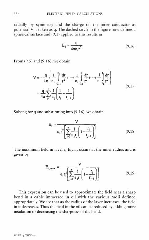
ELECTRIC FIELD CALCULATIONS336
radially by symmetry and the charge on the inner conductor atpotential V is taken as q. The dashed circle in the figure now defines aspherical surface and (9.1) applied to this results in
(9.16)
From (9.5) and (9.16), we obtain
(9.17)
Solving for q and substituting into (9.16), we obtain
(9.18)
The maximum field in layer i, Ei, max, occurs at the inner radius and isgiven by
(9.19)
This expression can be used to approximate the field near a sharpbend in a cable immersed in oil with the various radii definedappropriately. We see that as the radius of the layer increases, the fieldin it decreases. Thus the field in the oil can be reduced by adding moreinsulation or decreasing the sharpness of the bend.
© 2002 by CRC Press
ELECTRIC FIELD CALCULATIONS 337
9.2 ELECTRIC FIELD CALCULATIONS USING CONFORMALMAPPING
9.2.1 Physical Basis
In a region of space without charge, Maxwell’s electrostatic equation is
(9.20)
where D is the electric displacement. If the region has a uniformpermeability ε, then D=εE, where E is the electric field. Hence (9.20)becomes
(9.21)
Introducing a potential function V, where
(9.22)
we obtain from (9.21)
(9.23)
In 2-dimensions, using Cartesian coordinates, this last equation reads
(9.24)
The solution of (9.24), including boundary conditions, can then be usedto determine the electric field via (9.22).
Boundary conditions are generally of two types, Dirichlet orNeumann. A Dirichlet boundary condition specifies the voltage alonga boundary. This voltage is usually a constant as would beappropriate for a metallic surface. A Neumann boundary conditionspecifies the normal derivative along a boundary. The normalderivative is usually taken to be 0, which says that the equipotentialsurfaces (surfaces of constant V) or lines in 2-D intersect the boundaryat right angles. This type of boundary is often used to enforce asymmetry condition.
Functions satisfying equation (9.24) are called harmonic functions. Inthe theory of functions of a complex variable, analytic functions play a
© 2002 by CRC Press

ELECTRIC FIELD CALCULATIONS338
special role. These are functions which are continuous and differentiablein some region of the complex plane. It turns out that the real andimaginary parts of analytic functions are harmonic functions. Further,analytic mappings from one complex plane to another have propertieswhich allow a solution of (9.24) in a relatively simple geometry in onecomplex plane to be transformed to a solution of this equation in a morecomplicated geometiy in another complex plane. We briefly describesome of the important properties of these functions which are needed inthe present application. See reference [Chu60] for further details.
9.2.2 Conformal Mapping
Let z=x+iy denote the complex variable where is the unitimaginary. A function f(z) can be written in terms of its real andimaginary parts as
f(z)=u(x,y)+iv(x,y) (9.25)
where u and v are real functions of 2 variables. If f is analytic, it isdifferentiable at points z in its domain of definition. Since we are in thez-plane, the derivative can be taken in many directions about a givenpoint and the value must be independent of direction. Taking thisderivative in the x direction and then in the iy direction and equatingthe results, we obtain the Cauchy-Riemann equations
(9.26)
Differentiating the first of these equations with respect to x and thesecond with respect to y we have
(9.27)
Since the mixed partial derivatives on the right hand sides of theseequations are equal for differentiable functions, when we add theseequations we obtain
(9.28)
© 2002 by CRC Press

ELECTRIC FIELD CALCULATIONS 339
Thus u is a harmonic function. By differentiating the first of equations(9.26) with respect to y, the second with respect to x, and adding, wesimilarly find that v is a harmonic function.
The solution of the potential problem, equation (9.24) with boundaryconditions, is often needed in a rather complicated regiongeometrically. The idea behind using complex variable theory is toformulate the problem in a simpler geometric region where the solutionis easy and then use an analytic function to map the easy solution ontothe more complicated geometry of interest. The possibility of doing thisderives from several additional properties of analytic functions.
First of all, an analytic function of an analytic function is alsoanalytic. Since the real and imaginary parts of the original andcomposite functions are harmonic, this says that harmonic functions aretransformed into harmonic functions by means of analytictransformations. In terms of formulas, if f(z) is an analytic function of zand z=g(w) expresses z in terms of an analytic mapping from the w-plane, where w=u+iv, then f(g(w)) is an analytic function of w. The realand imaginary parts of f are transformed into harmonic functions of thenew variables u and v.
Given an analytic mapping from the z to w-plane, w=f(z), the inversemapping
z=F(w) is analytic at points where f'(z)=df/dz≠0. Moreover at suchpoints
(9.29)
This result will be useful in later applications to the electrostatic problem.Perhaps the most important characteristic of analytic mappings in
the present context is that they are conformal mappings. This meansthat if two curves intersect at an angle α in the z-plane, their images inthe w-plane under an analytic mapping w=f(z) intersect at the sameangle α at the transformed point. To see this, we use the fact that ananalytic function can be expanded about a point zo using a Taylor’sseries expansion
(9.30)
© 2002 by CRC Press

ELECTRIC FIELD CALCULATIONS340
where we assume that f'(zo)≠0. Writing ∆w=w-wo and ∆z=z-zo, this lastequation becomes
∆w=f'(zo)∆z (9.31)
If ∆z is an incremental distance along a curve in the z-plane , ∆w is thecorresponding incremental distance along the transformed curve in thew-plane (See Fig. 9.4). Since we can write any complex number in polarform,
(9.32)
in terms of its magnitude |z| and argument φ (9.31) can be expressed as
(9.33)
where ψo=argument (f'(z)) and α and β are shown in Fig. 9.4. Thus wesee from (9.33) that
β=ψo+α (9.34)
As ∆z and ∆w approach zero, their directions approach that of the tangentto their respective curves. Thus the angle which the transformed curvemakes with the horizontal axis β is equal to the angle which the originalcurve made with its horizontal axis α rotated by the amount ψo
Since ψo is characteristic of the derivative f'(Zo), which isindependent of the curve passing through zo, this says that any curvethrough zo will be rotated by the same angle ψo. Thus, since any twointersecting curves are rotated by the same angle under thetransformation, the angle between the curves will be preserved.
© 2002 by CRC Press

ELECTRIC FIELD CALCULATIONS 341
In terms of the electrostatic problem, this last mapping characteristicsays that a set of equipotential (non-intersecting) curves in onegeometry will remain non-intersecting in the transformed geometryobtained from the first by means of an analytic map. Similarly, theorthogonal relationship between the equipotentials and the electric fieldlines will be preserved in the new geometry.
Finally we need to look at the boundary conditions. If H is aharmonic function which is constant along some curve or boundary,
H(x,y)=C (9.35)
then, changing variables by means of z=f(w), this becomes, in the newvariables,
H(x(u,v),y(u,v))=C (9.36)
ie. a transformed curve along which H has the same constant value.Thus Dirichlet boundary conditions are transformed into Dirichletboundary conditions with the same boundary value along the transformedcurve.
A Neumann boundary condition means that the normal derivative ofH along the boundary vanishes. Since the normal derivative is thescalar product of the gradient and unit normal vector, the vanishing ofthis derivative means that the gradient vector points along theboundary, i.e. is tangential to it. However, the gradient vector isperpendicular to curves along which H is constant. Therefore these
Figure 9.4 Analytic mapping of a curve from the z to the w-plane
© 2002 by CRC Press

ELECTRIC FIELD CALCULATIONS342
curves of constant H are perpendicular to the boundary curve. Under aconformal mapping, this perpendicularity is preserved so that thetransformed boundary curve is normal to the transformed curves ofconstant H. Therefore the gradient of these transformed curves isparallel to the transformed boundary so that their normal derivativevanishes in the transformed geometry. Thus Neumann boundaryconditions are preserved under analytic transformations.
Since a solution of (9.24) which satisfies Dirichlet or Neumannboundary conditions is unique, under an analytic mapping, thetransformed solution subject to the transformed boundary conditionswill also be unique in the new geometry.
9.2.3 Schwarz-Christoffel Transformation
This transformation is an analytic mapping (except for a few isolatedpoints) from the upper half plane to the interior of a closed polygon.The closed polygon can be degenerate in the sense that some of itsvertices may be at infinity. This type of polygon includes the type ofinterest here.
Let us consider the general case as illustrated in Fig. 9.5. Part of thex-axis from x1 to xn= is mapped onto the boundary of a closed polygonin the w-plane. We have also drawn unit tangent vectors s and t alongcorresponding boundary curves in the z and w-planes. We showedearlier that the angle which the transformed curve makes with thehorizontal axis at a point is given by the angle which the original curvemakes with its horizontal plus the argument of the derivative of themapping. In this case, the original curve is along the x-axis in thepositive sense and so makes zero angle with this axis. Therefore thetransformed curve makes an angle with its axis given by arg(f'(z))where arg=argument of. Thus if the mapping has a constant argumentbetween two consecutive points along the x-axis, the transformedboundary curve will have a constant argument also and therefore be astraight line. However, as the w value moves along the boundarythrough a point wi where the polygon transitions from one side toanother, the argument of the tangent abruptly changes value. At thesepoints, the mapping cannot be analytic (or conformal). However, thereare only n such points for an n sided polygon.
© 2002 by CRC Press
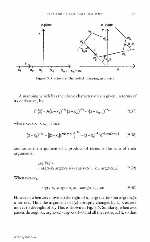
ELECTRIC FIELD CALCULATIONS 343
A mapping which has the above characteristics is given, in terms ofits derivative, by
(9.37)
where x1<x2<…< xn-1. Since
(9.38)
and since the argument of a product of terms is the sum of theirarguments,
arg(f'(z))= argA-k1 arg(z-x1)-k2 arg(z-x2)…kn–1 arg(z-xn–1) (9.39)
When z=x<x1,
arg(x-x1)=arg(x-x2)=…=arg(x-xn–1)=π (9.40)
However, when z=x moves to the right of x1, arg(x-x1)=0 but arg(x-xi)=π for i>2. Thus the argument of f(z) abruptly changes by k1 π as z=xmoves to the right of x1. This is shown in Fig. 9.5. Similarly, when z=xpasses through x2, arg(x-x1)=arg(x-x2)=0 and all the rest equal π, so that
Figure 9.5 Schwarz-Christoffel mapping geometry
© 2002 by CRC Press

ELECTRIC FIELD CALCULATIONS344
arg(f'(z)) jumps by k2π. These jumps are the exterior angles of the polygontraced in the w-plane. As such, they can be restricted to
-π≤kiπ≤π so that
-1≤ki≤1 (9.41)
Since the sum of the exterior angles of a closed polygon equals 2π, wehave for the point at infinity
knπ=2π-(k1+k2+…+kn–1)π (9.42)
so that
k1+k2+…+kn=2 (9.43)
Note that the point xn could be a finite point, in which case it must beincluded in equation (9.37). However, the transformation is simplifiedif it is at infinity.
To obtain the Schwarz-Christoffel transformation, we must integrate(9.37) to get
(9.44)
The complex constants A and B and the xi values can be chosen toachieve the desired map. There is some arbitrariness in the choice ofthese values and this freedom should be used to simplify the calculations.With this brief background, we now proceed to determine the mappingof interest here. Further details and proofs can be obtained by consultingRef. [Chu60] or other standard books on complex variables.
9.2.4 Conformal Map for the Electrostatic Field Problem
Fig. 9.6 shows the w-plane geometry of interest for the electrostatic fieldproblem and the corresponding z-plane boundary points. Note that someof the image points, w2, w3, and w5 are at infinity, albeit in differentdirections in the complex plane. In assigning values to x1, x2, x3, and x4,we have taken advantage of the symmetry in the w-plane geometry, Infact the coordinate systems were chosen to exploit this symmetry. Notethat, in Fig. 9.5 the positive direction for the exterior angles was chosenso that if we are moving along a side towards the next vertex, the angleincreases if we make a left turn and decreases if we turn towards the
© 2002 by CRC Press

ELECTRIC FIELD CALCULATIONS 345
right. In Fig. 9.6, as we move through the vertex w1 from w5, we turntowards the right by 90°, hence k1=-1/2. Moving through w2, we see thatwe make a 180° turn to the left, so k2=1. Passing through w3, we againmake a 180° left turn so k3=1. We turn right by 90° in going through w4,so k4=-1/2. The angular change through w5 is 180° to the left so k5=1.Thus k1+k2+k3+k4+k5=-1/2+1+1-1/2+1=2 as required.
The derivative of the transformation is, from (9.37),
(9.45)
where a>1. The integral can be carried out by writing
(9.46)
Substituting into (9.45), we get
(9.47)
Figure 9.6 Schwarz-Christoffel Transformation for the electrostatic problem
© 2002 by CRC Press

ELECTRIC FIELD CALCULATIONS346
Using tables of integrals and the definitions of the complex version ofthe standard functions (See Ref. [Dwi61]), we can integrate this to obtain
(9.48)
where ln is the natural logarithm. This solution can be verified bytaking its derivative.
In order to fix the constants, we must match the image points w1, w2,etc. to their corresponding x-axis points. Thus, we must get w1=-, whenx1=-a. Substituting into (9.48), we find
(9.49)
Since
ln z=ln|z|+iarg(z) (9.50)
(9.49) becomes
-=A[ln(2a)+iπ]+B (9.51)
since arg(-2a)=π. Similarly, we must have w4= correspond to x4=a.Substituting into (9.48), we find
(9.52)
Subtracting (9.51) from (9.52), we obtain 2=-iπA, so that
(9.53)
© 2002 by CRC Press

ELECTRIC FIELD CALCULATIONS 347
Adding (9.51) and (9.52), we obtain 0=2A ln(2a)+iπA+2B. Using (9.53)and solving for B, we get
(9.54)
Substituting A and B into (9.48), we obtain
(9.55)
The log terms can be combined, resulting in
(9.56)
Further manipulation of the log term leads to
(9.57)
Now, substituting ln(i)=ln(1)+i arg(i)=i π/2 and using the identity fromRef. [Dwi61],
(9.58)
where C is a complex number, (9.57) becomes,
© 2002 by CRC Press

ELECTRIC FIELD CALCULATIONS348
(9.59)
Substituting into (9.56), we get
(9.60)
To determine the constant a, we must use the correspondencebetween another set of points, such as x2, w2 or x3, w3. Using the x3, w3
pair, we note that as x approaches x3=1 from below, w must approach-ih. In (9.60) therefore let z= x→1 from below. Here we use anotherexpression for the complex inverse sin function [Dwi61],
(9.61)
where , and y≥0.
If=0 and x>1, p=1+x, q=x-1, and p+q=2x. If y=0 and x<-1, p=-(1-x), q=1-x, and p+q=-2x. If y=0 and |x|< 1, p=1+x, q=1-x, and p+q=2. This lattercase corresponds to the real sine function. Substituting z→1 into (9.60),we get
(9.62)
where the infinities must be interpreted in a limiting sense. Keeping thisin mind and using (9.61), we find
(9.63)
© 2002 by CRC Press

ELECTRIC FIELD CALCULATIONS 349
Since
(9.64)
we have
(9.65)
Substituting into (9.62), and neglecting finite real terms compared with, we get
(9.66)
Therefore √a2 – 1 =h/ and solving for a,
(9.67)
Thus (9.60) becomes
(9.68)
with a given by (9.67). Other points of correspondence can be checkedfor consistency by similar procedures.
9.2.4.1 Electric Potential and Field Values
In the w-plane which is the plane of interest for the electrostatic problem,the boundary values of the potential are shown in Fig. 9.7. Twoconductors are at potentials V1 and V2 relative to a plane at zero potential.This can be done without loss of generality, since if the plane were notat zero potential, its value could be subtracted from all the potentialvalues without altering the values of the electric field. The correspondingboundary values in the z-plane are also shown in Fig. 9.7. We wish tosolve the problem in the simpler z-plane geometry and then use the
© 2002 by CRC Press
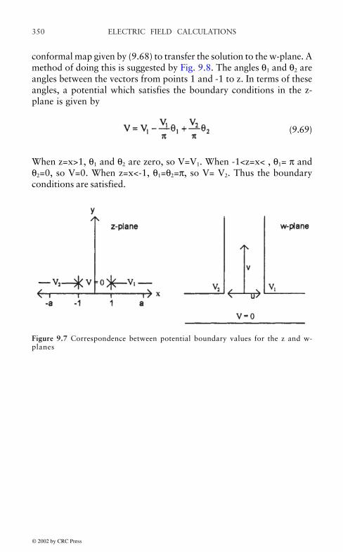
ELECTRIC FIELD CALCULATIONS350
conformal map given by (9.68) to transfer the solution to the w-plane. Amethod of doing this is suggested by Fig. 9.8. The angles θ1 and θ2 areangles between the vectors from points 1 and -1 to z. In terms of theseangles, a potential which satisfies the boundary conditions in the z-plane is given by
(9.69)
When z=x>1, θ1 and θ2 are zero, so V=V1. When -1<z=x< , θ1= π andθ2=0, so V=0. When z=x<-1, θ1=θ2=π, so V= V2. Thus the boundaryconditions are satisfied.
Figure 9.7 Correspondence between potential boundary values for the z and w-planes
© 2002 by CRC Press

ELECTRIC FIELD CALCULATIONS 351
We must now show that V is a harmonic function. Note that
θ1=arg(zθ1) , θ2=arg(z+1) (9.70)
Note also that
ln(z±1)=ln|z±1|+iarg(z±1) (9.71)
Since the log function is analytic, its real and imaginary componentsare harmonic functions as was shown previously for analytic functions.Thus θ1 and θ2 are harmonic and so is V since sums of harmonic functionsare also harmonic.
In terms of x and y where z=x+iy, (9.69) can be written
(9.72)
Since the transformation (9.68) is analytic except at a few points, theinverse transformation is defined and analytic at all points where w'=dw/dz≠0. Thus V can be considered a function of u, v through thedependence of x and y on these variables via the inverse transformation.This will enable us to obtain expressions for the electric field in the w-plane. We have,
Figure 9.8 The potential function in the z-plane
© 2002 by CRC Press

ELECTRIC FIELD CALCULATIONS352
(9.73)
Referring to (9.72), note that
(9.74)
Substituting c=±1, corresponding to the two terms in (9.72), and applyinga similar formula for the v derivative, we get for the electric fieldcomponents.
(9.75)
The derivatives in these formulas can be determined by means of (9.29),(9.45), and (9.53). Thus
(9.76)
Expressing this in terms of x and y and separating into real and imaginaryparts, we get
© 2002 by CRC Press

ELECTRIC FIELD CALCULATIONS 353
(9.77)
Now, using the uniqueness of the derivative when taken in the u or ivdirections which led to the Cauchy-Riemann equations mentioned earlier,we can write
(9.78)
This, together with (9.77) can be used to extract the appropriatederivatives for use in (9.75). Thus
(9.79)
© 2002 by CRC Press

ELECTRIC FIELD CALCULATIONS354
Thus the electric field in the w-plane can be expressed completely interms of x and y via (9.75) and (9.79). However, we must invertequation (9.68) to do this. The first step is to express (9.68) in terms of xand y and in terms of its real and imaginary parts. Thus we write thefirst sin-1 term, using (9.61),
(9.80)
where
The second sin-1 term in (9.68) can be written similarly,
(9.81)
where
with the upper sign referring to p1 and the lower sign to q1. Treating thethird sin-1 term in (9.68) similarly and separating into real and imaginaryparts, we get
© 2002 by CRC Press

ELECTRIC FIELD CALCULATIONS 355
(9.82)
where
The upper and lower signs refer to the p’s and q’s respectively.
© 2002 by CRC Press

ELECTRIC FIELD CALCULATIONS356
Given u and v, (9.82) can be inverted by means of a Newton-Raphson procedure. Using this method, the problem reduces to one ofsolving the following equations,
f1(x,y)=u(x,y)-uo=0
f2(x,y)=v(x,y)-vo=0(9.83)
where uo and vo are the desired coordinates at which to evaluate thefield in the w-plane. Since ∂f1/∂x=∂u/∂x, etc., the Newton-Raphsonequations for the increments ∆x, ∆y are
(9.84)
where we have used the Cauchy-Riemann equations (9.26). At eachiteration, we let xnew=xold+∆x and ynew=yold+∆y and stop when ∆x and ∆yare sufficiently small. The derivatives in (9.84) can be obtained by aprocedure similar to that used to derive (9.79).
9.2.4.2 Calculations and Comparison with a Finite Element Solution
A computer program was written to implement the above procedure forcalculating the electric field. According to the above formulas, the fieldis infinite at the corners of the conductors, however, because real cornersare not perfectly sharp, the field remains finite in practice. In transformerapplications, the conductors are usually covered with an insulating layerof paper and the remaining space is filled with transformer oil. Becausethe paper has a much higher breakdown stress than the oil, the field inthe oil is usually critical for design purposes, The highest oil fields willoccur at least a paper’s thickness away from the corner of the highestpotential conductor which we assume is at potential V1. We haveaccordingly calculated the field at the three points shown in Fig. 9.9which are a paper’s thickness, d, away from the corner of the V1 potentialconductor.
© 2002 by CRC Press

ELECTRIC FIELD CALCULATIONS 357
It should be noted that the presence of the paper, which has adifferent dielectric constant than oil, will modify the electric field. Ingeneral, it will increase it in the oil and decrease it in the paper. We willattempt to estimate this oil enhancement factor later. Here, we wish tocompare the analytic results as given by the above formulas with resultsfrom a finite element calculation without the presence of paper but withthe fields calculated at the points shown in Fig. 9.9, a paper’s distanceaway from the corner. The magnitudes of the fields, E, are compared,where
(9.85)
The results are shown in Table 9.1 for several different potentialcombinations and conductor separations. The agreement is very good,especially with the sharp corner finite element results. Also shown forcomparison are finite element results for a 0.02" radius on the corners.These are also reasonably close to the analytic results and show that thesharpness or smoothness of the corners is washed out at distances greaterthan or equal to a paper’s distance away. Although not shown in thetable, the field deep in the gap between the V1 and V2 conductors wasalso calculated with the analytic formulas and produced the expectedresult, E=(V2-V1)/.
Figure 9.9 Points near the corner of the highest potential conductor where theelectric field is calculated
© 2002 by CRC Press

ELECTRIC FIELD CALCULATIONS358
Also shown in Table 9.1 are the enhancement factors in parentheses,These are obtained by performing the finite element calculations withpaper having its normal dielectric constant ε=4.0 and then repeating itwith the paper layer given the dielectric constant of oil ε=2.2 and takingthe ratio of the field magnitudes in the two cases. This is normally greaterthan one, however in one case shown in the table it is 0.90. This isprobably due to discretization inaccuracies in the finite elementcalculation or possibly in pin-pointing the exact location of where toevaluate the field in the two cases since this was done with the cursor.Note that there seems to be a tendency for greater enhancement factors atthe corner point 2 than on either side of it for the sharp corner case.
The conformal mapping technique does not apply to the paper-oilsituation so other approximate approaches must be employed to accountfor the oil enhancement. The equipotential line plot for a finite elementcalculation with paper present is shown in Fig. 9.10, with a blow-up of
Table 9.1 Comparison of analytic and finite element electric field magnitudes atpoints 1, 2, 3 of Fig. 9.9. Enhancement factors are shown in parentheses.
© 2002 by CRC Press

ELECTRIC FIELD CALCULATIONS 359
Figure 9.10 Equipotential line plot from a finite element calculation showing thefull geometry for the conditions given in Table 9.1a with rounded comers
Figure 9.11 Equipotential line plot from a finite element calculation showing ablow-up of the region near the conductor’s corners for the same conditions asFig. 9.10
the region of interest shown in Fig. 9.11. This is for the conditions givenin Table 9.1a with rounded corners. Fig. 9.12 is a similar blow-up for theconditions in Table 9.1a with sharp metal corners.
© 2002 by CRC Press

ELECTRIC FIELD CALCULATIONS360
9.2.4.3 Estimating Enhancement Factors
For a paper-oil layering in a planar geometiy as shown in Fig. 9.13a,all the paper can be lumped into one layer for calculational purposes.Letting 1 refer to the paper layer and 2 to the oil layer, the enhancementfactor η=E/Eo, ie. the ratio of the fields with and without a paperlayer, is
(9.86)
where f1=1/, f2=2/ with =1+2 are the fractional lengths of materials1 and 2 respectively. It is assumed that when the paper is absent, it isreplaced by oil, keeping the total distance between the metal surfacesthe same.
Figure 9.12 Equipotential line plot from a finite element calculation for the sameconditions as Fig. 9.11 but with the conductors having sharp corners
© 2002 by CRC Press

ELECTRIC FIELD CALCULATIONS 361
In the cylindrical case, shown in Fig. 9.13b, the position of the paperlayer or layers is important in calculating the enhancement factors. Wewill assume that one paper layer is next to the inner conductor and onenext to the outer conductor. When additional layers are present, such aspressboard barriers, their position must be known and they can beincluded in the calculation. The oil enhancement factor for the situationshown in Fig. 9.13b is
(9.87)
The cylindrical enhancement factor is larger than the planar enhancementfactor for the same paper and oil layer thicknesses. It reduces to theplanar case when r1 becomes large.
The above enhancement factors refer to ideal geometries. For thegeometry of interest as shown in Fig. 9.9, the enhancement factorsreduce to the planar case for field points away from the corner and deepinto the V1-V2 gap or the V1–0 or V2–0 gaps. This is borne out by thefinite element calculations. However, near the corner, the geometry iscloser to the cylindrical case.
For a sharp corner, corresponding to r1=0, (9.87) shows that η→ε1/ε2=1.82 for the oil-paper case. This is an upper limit on the
Figure 9.13 Paper-oil configurations for (a) planar and (b) cylindrical geometriesresulting in enhanced fields in the oil compared with the all oil case
© 2002 by CRC Press

ELECTRIC FIELD CALCULATIONS362
enhancement factor and is more than enough to account for the sharpcorner enhancement factors shown in Table 9.1. For our purposes, therounded corner enhancement factors are the most relevant ones. Table9.1 shows that these are nearly the same for the 3 corner points.Treating the rounded corner case as a cylindrical geometry, we can taker1=0.02". It is less clear what radius to use for the outer conductor. InTable 9.2, we calculate the planar and cylindrical oil enhancementfactors for the two different gaps, where the outer conductor radius istaken to be the inner conductor radius plus the gap length which is orh for the two gaps (See Fig. 9.6). Thus, referring to Fig. 9.13b,
(9.88)
Note that the V1–0 gap has only one layer of paper. We also show aweighted cylindrical enhancement factor, which uses a weighted averageof the above two radii. The weighting is taken to be inverselyproportional to the radius so that the outer conductor closest to thecorner is given the highest weighting. This results in an effective outerconductor radius of
(9.89)
These weighted enhancements come closest to the corner enhancementsdetermined by the finite element calculations in most cases. We willtherefore use a cylindrical enhancement factor with this weighted outerconductor radius in our design calculations if it is above the V1"V2 gapplanar enhancement factor. Otherwise the V1"V2 gap planar enhancementfactor will be used.
Table 9.2 Calculated oil enhancement factors for the cases in Table 9.1.
© 2002 by CRC Press
ELECTRIC FIELD CALCULATIONS 363
The conformal mapping calculations of the electric field near thecorner of one of a pair of conductors at different potentials relative to aneighboring ground plane agree well with calculations obtained bymeans of a finite element program. Since the electric field is infinite at thecorner of a perfectly sharp conductor, the calculations were compared asmall distance from the corner, taken to be the thickness of a paper layerin an actual transformer winding. The finite element calculations weremade with sharp and rounded corners and the resulting fields were nearlythe same a paper’s thickness away from the corner. Since the oilbreakdown fields are the most critical in transformer design and theseoccur beyond the paper’s thickness, this result shows that a conformalmapping calculation is appropriate for determining these fields.
The only problem with the conformal mapping approach is that itdoes not take into account the different dielectric constants of oil andpaper. We have proposed a method to take these approximately intoaccount by means of an oil enhancement factor. By comparing with afinite element calculation, a formula was developed to obtain thisenhancement factor.
9.3 FINITE ELEMENT ELECTRIC FIELD CALCULATIONS
Finite element methods permit the calculation of electric potentials andfields for complicated geometries. Modern commercial finite elementcodes generally provide a set of drawing tools which allow the user toinput the geometry in as much detail as desired. More sophisticatedversions even allow parametric input so that changes in one or moregeometric parameters such as the distance between electrodes can beeasily accomplished without redoing the entire geometry. Both 2 and 3dimensional versions are available although the input to the 3D versionsis, of course, much more complicated. For many problems, a 2D geometrycan be an adequate approximation to the real configuration. 2D versionsusually allow an axisymmetric geometry by inputting a crosssection ofit. It this sense, it is really solving a 3D problem which happens to havecylindrical symmetry. The x-y 2D geometry is really modelling aninfinitely long object having the specified 2D cross-section.
The basic geometry which the user inputs is then subdivided into atriangular mesh. Smaller triangles are used in regions where thepotential is expected to change most rapidly. Larger triangles canadequately describe more slowly varying potential regions. Someprograms automatically perform the triangular meshing and, through
© 2002 by CRC Press

ELECTRIC FIELD CALCULATIONS364
an iterative process, even refine the mesh in critical regions until thedesired solution accuracy is achieved. When linear triangles are used,the potential is solved for only at the triangle nodes and a linearinterpolation scheme is used to approximate it inside the triangle. Forhigher order triangles, additional nodes are added per triangle andhigher order polynomial approximations are used to find the potentialinside the triangles. Some programs use only second order trianglessince these provides sufficient accuracy for reasonable computermemory and execution times.
Some art is required even for the geometric input. Very often,complete detail is unnecessary to a determination of the fields in criticalregions. Thus the user must know when it is reasonable to ignorecertain geometric details which are irrelevant to the problem. This notonly saves on the labor involved in inputting the geometry but it canalso considerably reduce required computer memory and solutiontimes.
Finite element programs require that the user input sources and theappropriate boundary conditions for the problem at hand. In the case ofelectric potential calculations, the sources are electric charges and theboundary conditions include specifying the voltage at one or moreelectrode surfaces. These are often the sufaces of metallic objects andthus have a constant potential throughout. It is therefore unnecessary tomodel their interiors. Typically, the program will allow the user todeclare such metallic objects nonexistant so that the solution is notsolved for over their interiors. Their surface, however, is still includedas an equipotential surface. Sometimes the equipotential surface is aboundary surface so it already has no interior. A metallic object canalso be allowed to float so that its potential is part of the problemsolution.
On external boundaries where no specification is made, theassumption is that these have natural or Neumann boundaryconditions. This means that the normal derivative of the potentialvanishes along them. This implies that the potential lines (in 2D) orsurfaces (in 3D) enter the boundary at right angles. These types ofboundary are usually used to express some symmetry condition. Forinstance a long conducting cylinder centered inside a rectangulargrounded box can by modelled by means of a circle inside the box.However, by symmetry, only a quarter of the geometry, centered on thecircle need be modelled and natural boundary conditions imposed onthe new boundaries created by isolating this region. This is depicted inFig. 9.14
© 2002 by CRC Press

ELECTRIC FIELD CALCULATIONS 365
The method works here because the potential lines are concentriccircles about the conducting cylinder and therefore enter the dotted lineboundaries in the 1/4 geometry at right angles. Although the problemdepicted in Fig. 9.14 is relatively simple to solve in the full geometry sothat the use of symmetry does not save much in input or solution times,this technique can save much effort when more complicated geometriesare involved.
Another boundary condition which some programs allow is theballoon boundary. This type of boundary is like specifying that theboundary doesn’t exist and the solution continues beyond it as if therewere empty space out to infinity in that direction. There is a practicalnecessity for this type of boundary condtition since the finite elementtechnique requires that the entire solution space of interest besubdivided into triangles or elements. When this solution space extendsinfinitely far or far enough that the geometric region of interest wouldbe dwarfed relative to the whole space, it is convenient to specify suchballoon boundaries rather that model vast regions of empty space.
We now give some examples of soving electrostatic problems with afinite element program. We use Ansoft’s Maxwell® 2D software[Ansoft]. The first is a varistor stack assembly shown in Fig. 9.15. Thisis an axisymmetric geometry. The varistors themselves are modelled astwo continuous cylinders separated by a metallic region in the centerwhich is floating. The ends consist of shaped metal electrodes to helpreduce the end fields. There are pressboard disks which mechanicallyhold the assembly together inside a pressboard cylinder. There is
Figure 9.14 Using symmetry to simplify the finite element problem
© 2002 by CRC Press
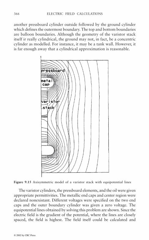
ELECTRIC FIELD CALCULATIONS366
another pressboard cylinder outside followed by the ground cylinderwhich defines the outermost boundary. The top and bottom boundariesare balloon boundaries. Although the geometry of the varistor stackitself ir really cylindrical, the ground may not, in fact, be a concentriccylinder as modelled. For instance, it may be a tank wall. However, itis far enough away that a cylindrical approximation is reasonable.
Figure 9.15 Axisymmetric model of a varistor stack with equipotential lines
The varistor cylinders, the pressboard elements, and the oil were givenappropriate permittivities. The metallic end caps and center region weredeclared nonexistant. Different voltages were specified on the two endcaps and the outer boundary cylinder was given a zero voltage. Theequipotential lines obtained by solving this problem are shown. Since theelectric field is the gradient of the potential, where the lines are closelyspaced, the field is highest. The field itself could be calculated and
© 2002 by CRC Press

ELECTRIC FIELD CALCULATIONS 367
displayed vectorially, if desired. The field can also be obtainednumerically at specified points along with the maximum field value.
The second example is of two long parallel cylindrical cables. Usingsymmetry, only the top half of one of these cables actually needs to bemodelled as shown in Fig. 9.16 This is an x-y geometry so that it isassumed to be infinitely long in the direction into the page. The metallicportion of the cable is surrounded by an insulating layer having acertain permittivity. The outside space is filled with oil, having adifferent permittivity. The metallic portion of the cylinder is declarednonexistant and its boundary is given half the potential differencebetween the two cylinders. This allows one to make the left boundaryline a zero potential line since it is assumed to bisect the distancebetween the two cylinders. The Top and right boundary lines areballoon boundaries. The bottom boundary line is unspecified (naturalboundary conditions assumed) since we are taking advantage of thesymmetry. The paper layer around the cable is actually subdivided intotwo layers separated by a thin aluminum layer which is floating.
Figure 9.16 Model of two parallel cylindrical cables, using symmetry to simplify it.The equipotential lines are shown.
© 2002 by CRC Press

ELECTRIC FIELD CALCULATIONS368
The equipotential solution lines are shown. They are closest togetheralong a line connecting the center lines of the two cylinders as might beanticipated so that the field is highest here. A closer inspection showsthat the highest field occurs in the oil at the surface of the paper alongthis line. As expected, the potential lines enter the bottom boundaryline at right angles.
© 2002 by CRC Press

369
10. LOSSES
Summary Transformer losses comprise a small percentage of the powerthroughput in a transformer. Yet these losses can produce localized heatingwhich can compromise its operation. It is important to be able to calculatethese losses at the design stage so that adequate cooling can be provided.In addition, such calculations and their parameter dependencies cansuggest ways of reducing these losses should that be necessary based oncost considerations or design feasibility. There are two main categoriesof losses, no-load and load losses. Noload losses are basically corelosses associated with energizing the transformer and driving flux throughthe core. Load losses are further subdivided into I2R losses and straylosses. The I2R losses are resistive losses in the windings and leads causedby the main current flow. The stray losses are the result of the stray fluxfrom the windings or leads impinging on metal parts such as the tankwalls, the clamps, and even the windings themselves, resulting in inducededdy currents. We present formulas or methods for obtaining these lossesin this report.
10.1 INTRODUCTION
Transformer losses are broadly classified as no-load and load losses.Noload losses occur when the transformer is energized with its ratedvoltage at one set of terminals but the other sets of terminals are opencircuited so that no through or load current flows. In this case, full fluxis present in the core and only the necessary exciting current flows inthe windings. The losses are predominately core losses due to hysteresisand eddy currents produced by the time varying flux in the core steel.Load losses occur when the output is connected to a load so that currentflows through the transformer from input to output terminals. Althoughcore losses also occur in this case, they are not considered part of theload losses. When measuring load losses, the output terminals areshorted to ground and only a small impedance related voltage isnecessary to produce the desired full load current. In this case, the corelosses are small because of the small core flux and do not significantlyadd to the measured losses.
© 2002 by CRC Press

LOSSES370
Load losses are in turn broadly classified as I2R losses due to Jouleheating produced by current flow in the coils and as stray losses due tothe stray flux as it encounters metal objects such as tank walls, clamps orbracing structures, and the coils themselves. Because the coil conductorsare often stranded and transposed, the I2R losses are usually determinedby the d.c. resistance of the windings. The stray losses depend on theconductivity, permeability, and shape of the metal object encountered.These losses are primarily due to induced eddy currents in these objects.Even though the object may be made of ferromagnetic material, such asthe tank walls and clamps, their dimensions are such that hysteresislosses tend to be small relative to eddy current losses.
Although losses are usually a small fraction of the transformed power(<0.5% in large power transformers), they can produce localized heatingwhich can compromise the operation of the transformer. Thus it isimportant to understand how these losses arise and to calculate them asaccurately as possible so that, if necessary steps can be taken at the designstage to reduce them to a level which can be managed by the coolingsystem. Other incentives, such as the cost which the customer attaches tothe losses, can make it worthwhile to find ways of lowering the losses.
Modern methods of analysis, such as finite element or boundaryelement methods, have facilitated the calculation of stray flux losses incomplex geometries. These methods are not yet routine in designbecause they require a fair amount of geometric input for each newgeometry. They can, however, provide useful insights in cases whereanalytic methods are not available or are very crude. Occasionally aparametric study using such methods can extend their usefulnessbeyond a specialized geometry. We will explore such methods, inparticular the finite element method, when appropriate. However, weare largely concerned here with analytic methods which can provideuseful formulas covering wide parameter variations.
10.2 NO-LOAD OR CORE LOSSES
Cores in power transformers are generally made of stacks of electricalsteel laminations. These are usually in the range of 0.23–0.46 mm (9–18 mils) in thickness and up to about 1 meter (40 inches) wide or aswide as can be accommodated by the rolling mill. Modern electricalsteels have a silicon content of about 3% which gives them a ratherhigh resistivity, ~ 50×10–8 Ω-m. Although higher silicon content canproduce even higher resistivity, the brittleness increases with silicon
© 2002 by CRC Press

LOSSES 371
content and this makes it difficult to roll them in the mill as well as tohandle them after. Special alloying, rolling, and annealing cycles producethe highly oriented Goss texture (cube on edge) with superior magneticproperties such as high permeability along the rolling direction. Thus itnecessary to consider their orientation in relation to the flux directionwhen designing a core.
Although the thinness of the laminations and their high resistivity aredesirable characteristics in reducing (classical) eddy current losses, the highdegree of orientation (>95%) produces large magnetic domains parallel tothe rolling direction as sketched in Fig. 10.1. The lines between domainswith magnetizations pointing up and down are called domain walls. Theseare narrow transition regions where the magnetization vector rotatesthrough 180°. During an a.c. cycle, the up domains increase in size at theexpense of the down domains during one part of the cycle and the oppositeoccurs during another part of the cycle. This requires the domain walls tomove in the direction shown in the figure for increasing up magnetization.As the domain walls move, they generate eddy current losses. These losseswere calculated by Ref. [Pry58] for the idealized situation shown in thefigure. They found that these losses were significantly higher than the lossesobtained from a classical eddy current calculation which assumes ahomogeneous mixture of many small domains. These non-classical lossesdepend on the size of the domains in the zero magnetization state wherethere are equal sized up and down domains. This is because the maximumdistance the walls move and hence their velocity depends on the zeromagnetization domain size. The larger this size and hence the greater thedomain wall’s velocity, the greater the loss.
Figure 10.1 Idealized magnetic domain pattern in highly oriented electrical steel.The up and down arrows show the magnetization direction. The side pointing smallarrows show the direction of domain wall motion for increasing up magnetization.v is their velocity.
© 2002 by CRC Press

LOSSES372
In order to decrease the non-classical eddy current losses, it istherefore necessary to reduce the domain size. This is accomplished inpractice by laser or mechanical scribing. A laser or mechanical stylus israstered across the domains (perpendicular to their magnetizationdirection) at a certain spacing. This introduces localized stress at thesurface since the scribe lines are not very deep. The domain size isdependent on the stress distribution in the laminations. Localizedstresses help to refine the domains. Thus, after scribing, the laminationsare not annealed since this would relieve the stress. Fig. 10.2 shows thedomain pattern in an oriented electrical steel sample before and afterlaser scribing. The domain patterns are made visible by means ofspecialized optical techniques. One can clearly see the reduction indomain size as a result of laser scribing in this figure. The losses werereduced by ~12% as a result of laser scribing in this example.
Figure 10.2 Effect of laser scribing on the domain wall spacing of oriented electricalsteel. Left side—before scribing, right side—after scribing. Courtesy of Armco Inc.With permission.
Another type of loss in electrical steels is hysteresis loss. This resultsfrom the domain walls encountering obstructions during their motion.At an obstruction, which can be a crystal imperfection, an occlusion orimpurity, or even a localized stress concentration, the domain wall ispinned temporarily. However, because of the magnetizing force drivingits motion, it eventually breaks away from the pinning site. This
© 2002 by CRC Press
LOSSES 373
process occurs very suddenly and the resulting high wall velocitygenerates localized eddy currents. These localized eddy current lossesare thought to be the essence of what are called hysteresis losses. Thusall losses in electrical steel are eddy current in nature. These hysteresislosses occur even at very low, essentially d.c., cycle rates. This isbecause, although the domain walls move very slowly until theyencounter an obstacle, the breakaway process is still very sudden. Thusin loss separation studies, the hysteresis losses can be measuredindependently by going to low cycle rates, whereas the total loss,including hysteresis, is measured at high cycle rates. In high qualityelectrical steel, the hysteresis and eddy current losses contribute aboutequally to the total loss.
The manufacturer or supplier of electrical steel generally providesthe user with loss curves which show the total loss per kilogram orpound as a function of induction at the frequency of interest, usually 50or 60 Hz. One of these curves is shown in Fig. 10.3a. This curve isgenerally measured under ideal conditions, i.e. low stress on thelaminations, and uniform, unidirectional, and sinusoidal flux in thelaminations, so that it represents the absolute minimum loss per kg or1b to be expected in service. Another useful curve which themanufacturer can provide is a curve of the exciting power per unitweight versus induction at the frequency of interest. A sample curve isshown in Fig. 10.3b. Again this is an idealized curve, but it can beuseful in estimating the power and current needed to energize thetransformer.
© 2002 by CRC Press

LOSSES374
Figure 10.3 Graphs of core loss and exciting power based on a polynomial fit todata provided by Armco Inc. With permission, TRAN-COR H® is a registeredtrademark of Armco Inc.
© 2002 by CRC Press

LOSSES 375
10.2.1 Building Factor
As mentioned previously, the specific core losses at the operating inductionprovided by the manufacturer are minimum expected losses so thatmultiplying by the core weight produces a total core loss lower than whatis measured in practice. The discrepancy is a result of the fact that stackedcores require joints where the induction must not only change directionbut must bridge a gap between different laminations and also becausestresses are produced in the steel due to cutting and stacking operations.There are other causes of this discrepancy such as burrs produced bycutting, but all of these can be lumped into a building factor which issimply a number which multiplies the ideal core loss to produce themeasured core loss. These building factors are generally in the range of1.2–1.4 and are roughly constant for a given core building practice.
Many attempts have been made to understand these extra losses,particularly in the region of the core joints, and have led to improvedjoint designs such as a step-lapped joint where the joint is madegradually in a step like manner. In a 3 phase core, studies have shownthat near the joints where the flux changes direction by 90°, theinduction vector rotates and higher losses are generated. Thus anotherapproach to calculating the building factor is to apply a multiplier tothe ideal losses for the amount of steel in the joint region only. This jointmultiplier would be higher that the average multiplier and could be ashigh as ~1.7. The advantage of this approach is that cores havingdifferent fractions of their overall weight in the joint regions shouldreceive more accurate average multipliers which reflect this difference.
10.2.2 Interlaminar Losses
The core laminations are coated with a glass-like insulating material.This is usually very thin, on the order of a few microns, to keep thespace factor reasonably high (>96%). Like any other material, the coatingis not a perfect insulator. Thus eddy currents, driven by the bulk flux inthe core, can flow across the stacked laminations which comprise thecore, i.e. normal to their surfaces. This is sketched in Fig. 10.4 for arectangular cross-section core. Of course the eddy current paths arecompleted within the laminations where the resistance is much lower.The coating must be a good enough insulator to keep these losses lowrelative to the normal intralaminar losses. The insulative value of thecoating is determined not only by the intrinsic resistivity of the coatingmaterial, which must be high, but also by its thickness. Although thethickness is generally not perfectly uniform, it should not vary so much
© 2002 by CRC Press
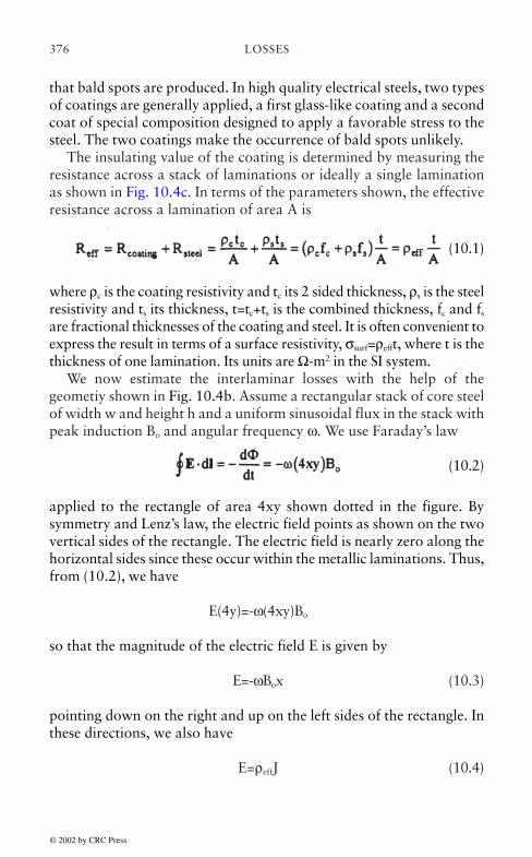
LOSSES376
that bald spots are produced. In high quality electrical steels, two typesof coatings are generally applied, a first glass-like coating and a secondcoat of special composition designed to apply a favorable stress to thesteel. The two coatings make the occurrence of bald spots unlikely.
The insulating value of the coating is determined by measuring theresistance across a stack of laminations or ideally a single laminationas shown in Fig. 10.4c. In terms of the parameters shown, the effectiveresistance across a lamination of area A is
(10.1)
where ρc is the coating resistivity and tc its 2 sided thickness, ρs is the steelresistivity and ts its thickness, t=tc+ts is the combined thickness, fc and fs
are fractional thicknesses of the coating and steel. It is often convenient toexpress the result in terms of a surface resistivity, σsurf=ρefft, where t is thethickness of one lamination. Its units are Ω-m2 in the SI system.
We now estimate the interlaminar losses with the help of thegeometiy shown in Fig. 10.4b. Assume a rectangular stack of core steelof width w and height h and a uniform sinusoidal flux in the stack withpeak induction Bo and angular frequency ω. We use Faraday’s law
(10.2)
applied to the rectangle of area 4xy shown dotted in the figure. Bysymmetry and Lenz’s law, the electric field points as shown on the twovertical sides of the rectangle. The electric field is nearly zero along thehorizontal sides since these occur within the metallic laminations. Thus,from (10.2), we have
E(4y)=-ω(4xy)Bo
so that the magnitude of the electric field E is given by
E=-ωBox (10.3)
pointing down on the right and up on the left sides of the rectangle. Inthese directions, we also have
E=ρeffJ (10.4)
© 2002 by CRC Press

LOSSES 377
where J is the current density and ρeff the effective resistivityperpendicular to the stack of laminations derived previously.
Figure 10.4 Interlaminar eddy currents produced by the bulk core flux
© 2002 by CRC Press

LOSSES378
The interlaminar losses are given by
(10.5)
where the volume integral is over the lamination stack, assumed uniformin the direction into the paper (which we take to have unit length). Thefactor of 1/2 comes from time averaging J which is assumed to beexpressed in terms of its peak value. Thus from (10.3)–(10.5), we get
(10.6)
where we have used ω=2πf. The specific loss (loss per unit volume) isgiven by
(10.7)
since we assumed unit length in the other dimension. To find the loss perunit weight or mass, divide by the density of the core steel in theappropriate units. Equation (10.7) is in the SI system where w is inmeters, Bo in Tesla, ρeff in Ω-m, f in Hz, and Pint in Watts/m3.
The interlaminar loss should be compared with the normal loss atthe same peak induction. For typical values of the parameters, it isgenerally much smaller than the normal loss and can be ignored. As anumerical example, let f=60 Hz, w=0.75 m, Bo=1.7 T, ρeff=20 Ω-m. Weget Pint=481 W/m3. The density of electrical steel is 7650 kg/m3 (16870lb/m3) so that Pint=0.063 W/kg (0.029 W/lb). This is a fairly small losscompared with the normal losses at 1.7 T of ~1.3 W/kg=0.60 W/lb.However, a high enough interlaminar resistance must be maintained toachieve these low losses.
© 2002 by CRC Press
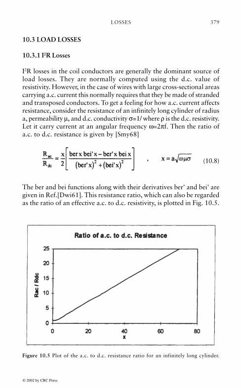
LOSSES 379
10.3 LOAD LOSSES
10.3.1 I2R Losses
I2R losses in the coil conductors are generally the dominant source ofload losses. They are normally computed using the d.c. value ofresistivity. However, in the case of wires with large cross-sectional areascarrying a.c. current this normally requires that they be made of strandedand transposed conductors. To get a feeling for how a.c. current affectsresistance, consider the resistance of an infinitely long cylinder of radiusa, permeability µ, and d.c. conductivity σ=1/ where ρ is the d.c. resistivity.Let it carry current at an angular frequency ω=2πf. Then the ratio ofa.c. to d.c. resistance is given by [Smy68]
(10.8)
The ber and bei functions along with their derivatives ber' and bei' aregiven in Ref.[Dwi61]. This resistance ratio, which can also be regardedas the ratio of an effective a.c. to d.c. resistivity, is plotted in Fig. 10.5.
Figure 10.5 Plot of the a.c. to d.c. resistance ratio for an infinitely long cylinder.
© 2002 by CRC Press
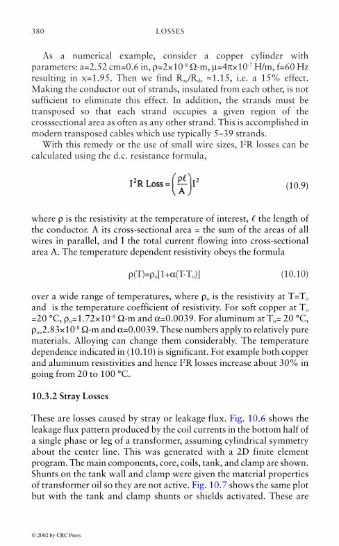
LOSSES380
As a numerical example, consider a copper cylinder withparameters: a=2.52 cm=0.6 in, ρ=2×10⁻⁸ Ω-m, µ=4π×10-7 H/m, f=60 Hzresulting in x=1.95. Then we find Rac/Rdc ≈1.15, i.e. a 15% effect.Making the conductor out of strands, insulated from each other, is notsufficient to eliminate this effect. In addition, the strands must betransposed so that each strand occupies a given region of thecrosssectional area as often as any other strand. This is accomplished inmodern transposed cables which use typically 5–39 strands.
With this remedy or the use of small wire sizes, I2R losses can becalculated using the d.c. resistance formula,
(10.9)
where ρ is the resistivity at the temperature of interest, the length ofthe conductor. A its cross-sectional area = the sum of the areas of allwires in parallel, and I the total current flowing into cross-sectionalarea A. The temperature dependent resistivity obeys the formula
ρ(T)=ρo[1+α(T-To)] (10.10)
over a wide range of temperatures, where ρo is the resistivity at T=To
and is the temperature coefficient of resistivity. For soft copper at To
=20 °C, ρo=1.72×10⁻⁸ Ω-m and α=0.0039. For aluminum at To= 20 °C,ρo=2.83×10⁻⁸ Ω-m and α=0.0039. These numbers apply to relatively purematerials. Alloying can change them considerably. The temperaturedependence indicated in (10.10) is significant. For example both copperand aluminum resistivities and hence I2R losses increase about 30% ingoing from 20 to 100 °C.
10.3.2 Stray Losses
These are losses caused by stray or leakage flux. Fig. 10.6 shows theleakage flux pattern produced by the coil currents in the bottom half ofa single phase or leg of a transformer, assuming cylindrical symmetryabout the center line. This was generated with a 2D finite elementprogram. The main components, core, coils, tank, and clamp are shown.Shunts on the tank wall and clamp were given the material propertiesof transformer oil so they are not active. Fig. 10.7 shows the same plotbut with the tank and clamp shunts or shields activated. These are
© 2002 by CRC Press

LOSSES 381
made of the same laminated electrical steel as the core. The shunts orshields divert the flux from getting into the tank or clamp walls so thatthe stray losses in Fig. 10.7 are much less than those in Fig. 10.6. Thestray flux pattern depends on the details of the winding sizes and spacings,the tank size, the clamp position, etc. The losses generated by this fluxdepend on whether shunts or shields are present as well as geometricand material parameters.
In addition to the coils’ stray flux, there is also flux produced by theleads. This flux can generate losses, particularly if the leads are close tothe tank wall or clamps. We should also mention losses in the tank walldepending on how the leads are taken out of the tank.
As Figs. 10.6 and 10.7 indicate, there is also stray flux within thecoils themselves. This flux is less sensitive to the details of the tank andclamp position or whether shunts or shields are present. Therefore,other methods besides finite elements, such as Rabin’s method whichuses a simplified geometry, can be used to accurately calculate this fluxin the coils. The coil flux generates eddy currents in the wires orindividual strands of cable conductors. The losses depend on the strandsize as well as its orientation relative to the induction vector and theinduction vector’s magnitude. The localized losses are thereforedifferent at different positions in the coil.
There are other types of stray loss which occur either in case of anunusual design or when a manufacturing error occurs. In the lattercategory, extra losses are generated when a cross-over or transpositionis missed or misplaced in a coil made of two or more wires or cables inparallel.
We will examine these various types of stray loss here, derivinganalytic formulas or procedures for evaluating them where possible orrelying on finite element studies or other numerical methods ifnecessary.
© 2002 by CRC Press
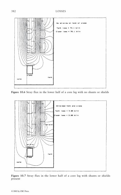
LOSSES382
Figure 10.6 Stray flux in the lower half of a core leg with no shunts or shields
Figure 10.7 Stray flux in the lower half of a core leg with shunts or shieldspresent
© 2002 by CRC Press

LOSSES 383
10.3.2.1 Eddy Current Losses in the Coils
In order to study the effect of stray flux on losses in the coils, we examinean individual wire or strand which could be part of a transposed cable.This is assumed to have a rectangular cross-section. The magnetic fieldat the site of this strand segment will point in a certain direction relativeto the strand’s orientation. This vector can be decomposed into componentsparallel to each side of the rectangular cross-section as shown in Fig.10.8a. (In a transformer, there is little or no magnetic fields directedalong the length of the wire.) We analyze the losses associated with eachcomponent of the magnetic field separately and add the results. This isaccurate to the extent that the eddy currents associated with the differentfield components do not overlap. We will see in the following that theeddy currents tend to concentrate along the sides of the rectangular strandto which the field component is parallel. Thus the eddy current patternsassociated with the two field components do not overlap significantly sothat our method of analysis is reasonably accurate.
Figure 10.8 Geometry for calculating losses in a conducting strand due to anexternal magnetic field
© 2002 by CRC Press

LOSSES384
Consider the losses associated with the y-component of an externalmagnetic field as shown in Fig. 10.8b, where the coordinate system andgeometric parameters are indicated. We assume an idealized geometrywhere the strand is infinitely long in the z-direction. This implies thatnone of the electromagnetic fields have a z dependence. We furtherassume that the magnetic field, both external and internal, has only aycomponent. Applying Maxwell’s equations in this coordinate systemand with these assumptions, we obtain in the SI system.
(10.11)
where µ is the permeability, E the electric field, and H the magneticfield. We have ignored the displacement current term which is onlyimportant at extremely high frequencies. In the metallic conductor, wehave Ohm’s law in the form
(10.12)
where µ is the electrical conductivity. There is only a z-component to Jand E. Combining (10.11) and (10.12), we obtain
(10.13)
where Hy is a function of x and t.Let Hy have a sinusoidal time dependence of the form
Hy(x,t)=Hy(x)ejωt (10.14)
Then (10.13) becomes
© 2002 by CRC Press

LOSSES 385
(10.15)
Hy is only a function of x in (10.15). Solving (10.15) with the boundarycondition that Hy=Ho at x=±b/2 where b is the strand width normal tothe field direction and Ho is the peak amplitude of the external field,we get
(10.16)
and from (10.11)
(10.17)
The eddy current loss per unit length in the z direction is
(10.18)
where c is the strand dimension along the field direction. The factor of1/2 comes from taking a time average and using peak values of thefield. The integration through only half the thickness is possible becauseof the symmetry of the integrand. Note that, from (10.15),
(10.19)
Using this expression for k, we have the identities.
(10.20)
© 2002 by CRC Press

LOSSES386
Substituting into (10.18), integrating, and dividing by the cross-sectionalarea, we get the specific eddy current loss (loss/unit volume) as
(10.21)
This is in Watts/m3 in the SI system. Simply divide by the density in thissystem to get the loss per unit mass or weight.
This last equation applies over a broad frequency range, up to whereradiation effects start becoming important. At the low frequency end,which applies to transformers at power frequencies (small qb), thisreduces to
(10.22)
where we have used σ=1/ρ, where ρ is the resistivity, ω=2πf, where f isthe frequency, and Bo=µHo.
As a numerical example, let Bo=0.05T which is a typical leakageinduction value in the coil region, ρ=2×10⁻⁸ Ω-m, σ=5×10⁷ (Ω-m)-1,ω=2πf=2π(60) rads/sec, b=6.35×10⁻³ m (0.25 in), µ=4π×10–7 H/m. Thenq=108.8 m-1 and qb=0.691. This is small enough that the small qb limitshould apply. Thus we get from (10.22), Pec=2.985× 10⁴ W/m3. Theexact formula (10.21) yields Pec=2.955×10⁴ W/m3. Using the density ofcopper dCu=8933 kg/m3, we obtain Pec=3.35 W/kg=1.52 W/1b. The I2Rloss on a per volume basis associated with an rms current of 3×10⁶ A/m2=1935 A/in2 (a typical value) in a material (copper) of the aboveresistivity, is 1.8×10⁵ W/m3 so that the eddy current loss amounts toabout 17% of the I2R losses in this case.
The losses given by (10.21) or (10.22) must be combined with thelosses given by a similar formula with Ho or Bo referring to the peak valueof the x-component of the field and with b and c interchanged. This willgive the total eddy current loss density at the location of the strand. Amethod of calculating the magnetic field or induction at various locationsin the coils is needed. From the axisymmetric field calculation (flux map)given in Figs. 10.6 and 10.7, we obtain values of the radial and axialcomponents of the field. These replace the x, y components in the lossformulas given above. These loss densities will differ in different parts ofthe winding. To obtain the total eddy current loss, an average loss densitycan be obtained for the winding and this multiplied by the total weight or
© 2002 by CRC Press

LOSSES 387
volume of the winding. However, in determining local windingtemperatures and especially the hot spot temperature, a knowledge ofhow these losses are distributed is necessary.
From (10.17), (10.19), and (10.20), we can obtain the eddy currentloss density as a function of position in the strand,
(10.23)
This vanishes at the center of the strand (x=0) and is a maximum at thesurface (x=± b/2). The parameter q measures how fast this drops offfrom the surface. The fall off is more rapid the larger the value of q. Thereciprocal of q is called the skin depth and is given by
(10.24)
For copper at ~ 60 °C, σ=5×10⁷ (Ω-m)”1, and f=60 Hz, we get δ=0.92cm=0.36 in. For aluminum at ~60 °C, σ=3×10⁷ (Ω-m)-1 , and f =60 Hz,we get δ=1.19 cm=0.47 in. Thus the skin depth is smaller for copperthan aluminum which means that the eddy currents concentrate moretowards the surface of copper than aluminum.
The high frequency limit of (10.21) (large qb) is
(10.25)
This increases as the square root of the frequency.
10.3.2.2 Tieplate Losses
The tieplate (also called flitch plate) is located just outside the core inthe space between the core and innermost winding. It is a structuralplate which connects the upper and lower clamps. Tension in this plateprovides the clamping force necessary to hold the transformer togethershould a short circuit occur. It is usually made of magnetic steel orstainless steel and could be subdivided into several side by side verticalplates to help reduce the eddy current losses. Fig. 10.9 shows a schematicdiagram of one of the tieplates associated with one leg. There is anotheron the opposite side of the core leg. These generally have a rectangularcross-section.
© 2002 by CRC Press

LOSSES388
Since the flux plots in Figs. 10.6 and 10.7 are for a 2 dimensional,axisymmetric geometry, it was not possible to include the tieplate. (Thiswould have made it a solid cylinder around the core.) However, the fluxpattern shown in the figures should not be greatly altered by theirpresence since they occupy a fairly small fraction of the core’scircumference. As the flux pattern in the figures show, the flux isprimarily radial at the location of the tieplate. However, with an actualtieplate present, there will be some axial flux carried by the tieplate.This will depend on the permeability of the tieplate relative to that ofthe core. We can estimate the axial tieplate flux by reference to Fig.10.10 where we show two side by side solids of permeabilities µ1, µ2 andcross sectional areas A1, A2 carrying flux. We assume that the coilsproducing this flux create a common magnetic field H at the location ofthe solids. (The field inside an ideal solenoid is a constant axial field.)
Figure 10.9 Tieplate location in a transformer
© 2002 by CRC Press

LOSSES 389
The induction inside each solid is given by
(10.26)
so that
(10.27)
Using this last expression, we can estimate the induction in the tieplate.We can use the ratio of relative permeabilities in the above formula.These are a.c. permeabilities which we take to be ~5000 for the coreand ~200 for a magnetic steel tieplate. With a core induction of 1.7Tesla which is typical, we find that Bmag t.p.=0.04 Bcore=0.068 T. For astainless steel tieplate of relative permeability=1, we obtain Bs.s. t.p.=0.0002 Bcore=0.00034 T. Thus the axial induction is not insignificant fora magnetic steel tieplate but ignorable for a stainless steel one.
Let us first look at the losses due to the radial induction since theseare common to both magnetic and stainless steel tieplates. We havestudied these losses using a 2D finite element analysis. Fig. 10.11 showsa flux plot for a magnetic steel tieplate, assuming a uniform 60 Hzsinusoidal flux density far from the plate. The plate is assumed to beinfinitely long in the dimension perpendicular to the page. Only 1/2 thegeometry is modeled, taking advantage of symmetry about the lefthand axis. The plate rests directly on a material of high permeability,
Figure 10.10 Dissimilar magnetic materials in a common magnetic field
© 2002 by CRC Press

LOSSES390
the core. The loss density contours are shown in Fig. 10.12. Thisindicates that the eddy currents are concentrated near the surface due tothe skin effect. Fig. 10.13 shows a similar flux plot for a stainless steeltieplate. Note that there is little eddy current screening so the fluxpenetrates the plate without much distortion. Fig. 10.14 shows the lossdensity contours for the stainless steel tieplate. There is much lesssurface concentration of the eddy currents. Although we only calculateeddy current losses with a finite element program, the hysteresis lossesin a magnetic steel tieplate make up only a small fraction of the totallosses for typical tieplate dimensions.
The finite element study was repeated for different tieplate widths(perpendicular to the flux direction) while keeping the thickness (alongthe flux direction) constant at 0.95 cm (3/8 in). The results are shown inFig. 10.15, where the loss per unit length in the axial direction and perT2 are plotted. To get the actual loss multiply the ordinate by thetieplate length and by the square of the radial induction in T2. Fig.10.16 shows the same information as plotted in Fig. 10.15 but on a log-log plot. This allows the extraction of the power dependence of the losson the width of the tieplate. The material parameters assumed were, formagnetic steel: resistivity=25×10-8 Ω-m and relative permeability=200,for stainless steel: resistivity=75×10-8 Ω-m and relative permeability=1.We obtain for the losses
(10.28)
© 2002 by CRC Press

LOSSES 391
Figure 10.11 Flux lines for a magnetic steel tieplate in a uniform 60 Hz magneticfield normal to its surface. The tieplate rests on a high permeability core. Only 1/2 the geometry is modeled.
Figure 10.12 Loss density contours for the magnetic steel tieplate shown in Fig.10.11.
© 2002 by CRC Press
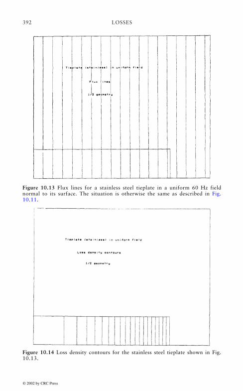
LOSSES392
Figure 10.13 Flux lines for a stainless steel tieplate in a uniform 60 Hz fieldnormal to its surface. The situation is otherwise the same as described in Fig.10.11.
Figure 10.14 Loss density contours for the stainless steel tieplate shown in Fig.10.13.
© 2002 by CRC Press

LOSSES 393
Figure 10.15 Losses for 0.95 cm (3/8 in) thick tieplates made of magnetic andstainless steel versus the tieplate width. The tieplates are in a uniform 60 Hzmagnetic field directed normal to the tieplate surface.
Figure 10.16 Same as Fig. 10.15 but on a log-log scale.
© 2002 by CRC Press

LOSSES394
The stainless steel finite element study shows that the magnetic fieldand eddy currents inside the tieplate have nearly the same direction andgeometry dependence as was assumed for the eddy current loss inconducting strands. Therefore if we multiply the loss density given in(10.21) or (10.22) by the plate’s cross sectional area, we should getnearly the same result as given above for stainless steel. We note that wshould be substituted for b in the previous formulas. Using the small qbformula (10.22), and putting in the stainless steel parameters, we obtain
which is close to the result given above in SI units. We do not expectexact agreement since qb(=qw) for stainless at w=0.127 m (5 in) is ~2.26which is a little above the range of validity of the small qb formula.
In the case of magnetic steel, as Figs. 10.11 and 10.12 show, theconditions under which the strand eddy current losses were developeddo not hold. The field is not strictly y-directed (radially directed) and itdoes not depend only on x (the width direction). We should note that,according to Fig. 10.15, the losses per unit length due to radial flux arehigher in stainless steel tieplates than in magnetic steel plates for thesame width and thickness. However, for magnetic steel tieplates, weneed to add on the losses due to the axial flux they carry.
We can estimate the losses in the tieplate due to axial flux byresorting to an idealized geometry. We assume the tieplate is infinitelylong and the flux is driven by a uniform axial magnetic field parallel tothe tieplate’s surface. We are also going to assume that its width is muchgreater than its thickness, in fact we assume an infinite width. Thus, asshown in Fig. 10.17, the only relevant dimension is the y-dimensionthrough the sheet’s thickness. The eddy currents will flow primarily inthe x direction. We ignore their return paths in the y-direction which aresmall compared to the x-directed paths.
© 2002 by CRC Press
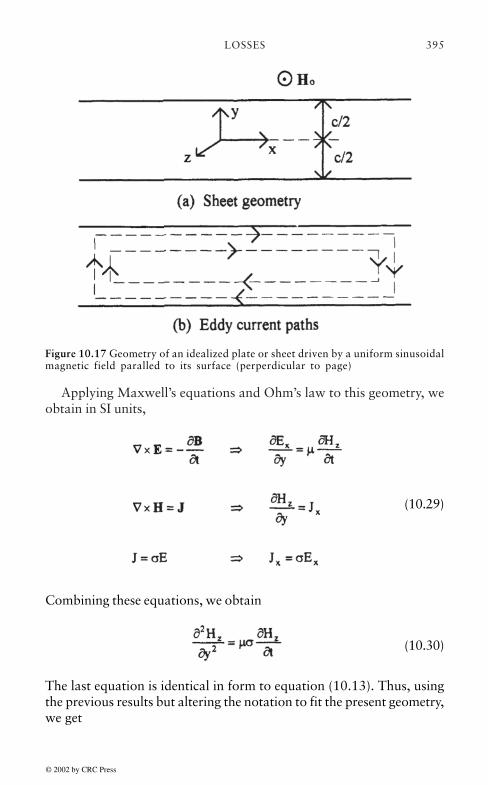
LOSSES 395
Applying Maxwell’s equations and Ohm’s law to this geometry, weobtain in SI units,
(10.29)
Combining these equations, we obtain
(10.30)
The last equation is identical in form to equation (10.13). Thus, usingthe previous results but altering the notation to fit the present geometry,we get
Figure 10.17 Geometry of an idealized plate or sheet driven by a uniform sinusoidalmagnetic field paralled to its surface (perperdicular to page)
© 2002 by CRC Press

LOSSES396
(10.31)
and
(10.32)
This is a loss per unit volume (W/m3) in the tieplate due to axial flux.Since the eddy currents generating this loss are at right angles to theeddy currents associated with the radial flux normal to the surface,there is no interference between them and the two losses can be added.
For magnetic steel at 60 Hz with µr=200, µ=µr 4π×10-7 H/m, σ=4×10⁶
(Ω-m)-1 and c=9.52×10⁻³ m (0.375 in), we have qc=4.15. This is largeenough that (10.32) must be used without taking its small qc limit.Substituting the parameters just given for magnetic steel and usingBo=0.07 T (Ho=Bo/µ), we obtain Ptp,axial=925 W/m3=0.12 W/kg, where wehave used 7800 kg/m3 for the density of magnetic steel. The radial fluxloss formula for magnetic steel given previously, equation (10.28), mustbe divided by the cross sectional area for comparison with the aboveloss. We find, using Brms=0.1 T, w=0.127 m (5 in) and the previous valuefor c, Ptp,radial=1552 W/m3=0.20 W/kg. Thus it appears that for amagnetic steel tieplate, the loss associated with the axial flux iscomparable with the loss associated with the radial flux. In any event,these two losses must be added to get the total loss. Since stainless steeltieplates have virtually no axial flux loss, the net effect is that magneticsteel tieplates could have a higher loss than comparably sized stainlesssteel tieplates.
Since the axial flux loss is, to first order, independent of tieplatewidth, the width dependence of the total magnetic steel tieplate lossesshould not be as pronounced as that for stainless steel ones. Thussubdividing the tieplates either with axial slots or into separate plateswill not be as effective for magnetic steel as compared with stainlesssteel tieplates in reducing the losses. However, one benefit of magneticsteel tieplates, not shared by stainless steel ones, is that they keep theradial flux from passing through them into the core steel. (CompareFigs. 10.11 and 10.13.) They do, however, concentrate the radial fluxreaching the core to the regions near the outer edges of the tieplatewhere oil cooling should be more effective.
© 2002 by CRC Press

LOSSES 397
10.3.2.3 Tieplate and Core Losses Due to Unbalanced Currents
There is a rather specialized type of loss which can occur in transformerswhich have a large unbalanced net current flow. The net current is thealgebraic sum of the currents flowing in all the windings. This, incontrast with the net Ampere-turns which are always nearly exactlybalanced, can be unbalanced. To visualize the magnetic effect of awinding’s current, consider a cylindrical (solenoidal) winding carryinga current which flows in at the bottom and out at the top. Outside thewinding, the net upward current appears equally distributed aroundthe cylinder. The magnetic field outside the cylinder associated withthis current is the same as that produced by the current flowing alongthe centerline of the cylinder. In a core-form transformer, some of thewindings carry current up and some down. The algebraic sum of allthese currents can be considered as being carried by one cylinder ofradius equal to a weighted average of the contributing windings,weighted by their current magnitudes. Outside this radius, the field isthat of a straight wire along the centerline earning the algebraic sum ofthe currents.
The field around a long straight wire carrying a current I is directedalong concentric circles about the wire and has magnitude in SI units,
(10.33)
where r is the radial distance from the centerline and ϕ, the azimuthalangle, indicates that the field is azimuthally directed. We are using boldfaced type here to indicate that the current is a phasor quantity, since weare considering a 3 phase transformer on a single 3 phase core. Thisfield cuts through the transformer core windows as shown in Fig. 10.18.The alternating flux passing through the core window induces a voltagearound the core structure which surrounds the window. The tieplates,including their connection to the upper and lower clamps, make a similarcircuit around the core windows so that voltage is induced in them aswell.
We can calculate the flux due to the coil in Fig. 10.18a through theleft hand window, labeled 1 in the figure, Φa1, using (10.33)
(10.34)
© 2002 by CRC Press

LOSSES398
where µo is the permeability of oil (air)=4π×10-7 H/m, h the effectivewinding height, d the leg center to center distance, and rw the effectivewinding radius, h can be obtained as a weighted average of thecontributing windings as was done for rw. We have integrated all theway to the centerline of the center leg. This is an approximation as theflux lines will no doubt deviate from the ideal radial dependence givenin (10.33) near the center leg. The flux through window 2 due to thephase a current, Φa2, is similarly
(10.35)
Using the same procedure, we find the flux through the two windowsdue to phases b and c shown in Fig. 10.18 b, c
(10.36)
Thus the net fluxes through windows 1 and 2 are
(10.37)
© 2002 by CRC Press

LOSSES 399
Figure 10.18 Field around a cylindrical winding located on a transformer leg andcarrying a net upward current
© 2002 by CRC Press

LOSSES400
Considering Ia, Ib, Ic to be a positive sequence set of currents andperforming the phasor sums above, we get
(10.38)
From Faraday’s law, the voltages induced by the two fluxes are
(10.39)
The direction of these voltages or emf’s s is given by Lenz’s law, i.e.they try to oppose the driving flux,. We can assume that V1 is the referencephasor and thus drop the minus sign and phase factor from its expression.Then V2 is given by (10.39) with a phase of θ2-θ1 relative to the referencephasor.
The induced voltages will attempt to drive currents through thetieplates and core in loops surrounding the two windows. This will beopposed by the resistances of the tieplates and core and by the self andmutual inductances of the metallic window frames whether formed ofcore sections or of tieplate and clamp sections. We can treat these aslumped parameters, organized into the circuits of Fig. 10.19. There are3 circuits involved since there are two tieplate circuits on either side ofthe core plus the core circuit. These are essentially isolated from eachother except for coupling through the mutual inductances. Although thetieplate circuits share the top and bottom clamps in common, they aresufficiently symmetric that they can be regarded as separate circuits.We assume that magnetic coupling exists only between window 1 loopsor window 2 loops but not between a window 1 loop and a window 2loop. To make the circuit equations more symmetric, we havepositioned V2 in the circuit in such a way that it is necessary to take thenegative of the expression in (10.39).
© 2002 by CRC Press

LOSSES 401
Thus we have for the voltage sources in the circuits of Fig 10.19,assuming V1 is the reference phasor,
(10.40)
where f is the frequency in Hz.Using the notation of Fig. 10.19 and assuming sinusoidal conditions,
we can write the circuit equations
Figure 10.19 Equivalent circuits for tiepiates and core driven by voltages inducedthrough unbalanced currents
© 2002 by CRC Press

LOSSES402
(10.41)
These can be organized into a matrix equation and solved for thecurrents, using complex arithmetic. However, it is possible to solvethem using real arithmetic by separating the vectors and matrix intoreal and imaginary parts. Thus, given a matrix equation
V=MI (10.42)
where V and I are complex column vectors and M a complex matrix,write
(10.43)
Here bold faced type is doing double duty in indicating both vector andphasor quantities. Substituting this separation into real and imaginaryparts into (10.42), we get
(10.44)
This reduces to two separate equations,
(10.45)
which can be organized into a larger matrix equation
© 2002 by CRC Press

LOSSES 403
(10.46)
Here the separate entries are real vectors and matrices. Thus we havedoubled the dimension of the original matrix equation (10.41) from 6 to12 but this is still small, considering the power of modern computers.
The remaining issues concern how to evaluate the resistances and theself and mutual inductances in (10.41). The resistance of a tieplate, R,can simply be taken as its d.c. resistance since it has a relatively smallthickness. We can ignore the resistance of the clamps since these shouldhave a much larger cross-sectional area than the tieplates. The core,with its fairly large radius and high permeability will have an enhanceda.c. resistance relative to its d.c. value. It can be estimated from Fig.10.5, using an effective a.c. permeability and conductivity.
Since we do not expect extreme accuracy in this calculation, in viewof the approximations already made, we can use approximate formulasfor the self and mutual inductances. For example, Ref. [Gro73] gives aformula for the inductance of a rectangle of sides a and b made of wirewith a circular cross-section of radius r and relative permeability µr
which is, in SI units,
(10.47)
L is in Henrys and lengths are in meters in the above formula. Thisformula can be applied directly to calculate the inductance of the corewindow. By defining an effective radius, it can be applied to the tieplateloop as well. In calculating the core inductance, remember that the corecurrent generates magnetic field lines in the shape of concentric circlesabout the core centerline so that the appropriate relative permeability isroughly the effective permeability perpendicular to the laminations. Fora stacking factor of 0.96 and infinitely permeable laminations, the effectiveperpendicular permeability is µr=25. Similarly, the effective tieplatepermeability is close to 1.0 for both magnetic and stainless steel tieplates.
The mutual inductance terms are not quite so important so that aneven cruder approximation may be used. Ref. [Gro73] gives anexpression for the mutual inductance between two equal coaxial squares
© 2002 by CRC Press

LOSSES404
of thin wire which are close together. Letting s be the length of the side ofthe squares and d their separation, the mutual inductance, in SI units, is
(10.48)
In this equation, M is in Henrys and lengths in meters. With a littleimagination, this can be applied to the present problem. Once (10.41) orits equivalent (10.46) is solved for the currents, the losses, which are I2Rtype losses, can be calculated. As a numerical example, we found thecore and tieplate losses due to an unbalanced current of 20,000 Amps rmsat 60 Hz in a transformer with the following geometric parameters,
The tieplates were actually subdivided into three plates in the widthdirection but this does not affect the calculation. For magnetic steeltieplates, the calculated core loss was 11 Watts and the total tieplateloss was 1182 Watts. For stainless steel tieplates, the calculated coreloss was 28 Watts and the total tieplate loss was 2293 Watts. For themagnetic steel case, the current in the core legs was about 200 Ampsand in the tieplates about 600 Amps. For the stainless steel case, thecurrent in the core legs was about 300 Amps and in the tieplates about500 Amps. The stainless steel losses are higher mainly because of thehigher resistivity of the material coupled with the fact that theimpedances, which limit the currents, are mainly inductive and hencenearly the same for the two cases.
10.3.2.4 Tank and Clamp Losses
Tank and clamp losses are very difficult to calculate accurately. Herewe are referring to the tank and clamp losses produced by the leakageflux from the coils, examples of which are shown in Figs. 10.6 and10.7. The eddy current losses can be obtained from the finite elementcalculation, however the axisymmetric geometry is somewhat simplistic
Winding height (h) 0.813 m (32 in)Winding radius (rw) 0.508 m (20 in)Leg center-center distance (d) 1.727 m (68 in)Core radius 0.483 m (19 in)Tieplate and core height 5.08 m (200 in)Tieplate width 0.229 m (9 in)Tieplate thickness 9.525×10⁻³ m (0.375 in)
© 2002 by CRC Press

LOSSES 405
if we really want to model a 3 phase transformer in a rectangular tank.Modern 3D finite element and boundary element methods are beingdeveloped to solve eddy current problems and should be widely availablein the near future. In fact, some of these codes are already on the market.They are not, however, in routine use largely because of the complexityof 3D versus 2D modeling as well as computation time and memorylimitations. These problems should disappear with time and fully 3Dcalculations of losses should become routine.
In the meantime, much can be done with a 2D approach. We refer to astudy in Ref. [Pav93] where several projection planes in the 3D geometrywere chosen for analysis with a 2D finite element program. The lossescalculated with this approach agreed very favorably with test results. Asthat study and our own show, 2D models allow one to quickly asses theimpact on losses of design changes such as the addition of tank and/orclamp shunts made of laminated electrical steel or the effect on losses ofaluminum or copper shields at various locations. In fact the losses in Fig.10.7 with tank and clamp shunts present were dramatically reducedcompared with those in Fig. 10.6 where no shunts are present. While thereal losses may not show as quantitative a reduction, the qualitativeeffect is real. Another study which was done very quickly, using theparametric capability of the 2D modeling, was to asses the impact ofextending the clamp shunts beyond the top surface of the clamp. Wefound that some extension was useful in reducing the losses caused bystray flux hitting the vertical side of the clamp.
An example of where a 3D approach is crucial in understanding theeffect of design options on losses concerns the laminated steel shunts onthe clamps. The side clamps extend along all three phases of atransformer as shown in the top view of Fig. 10.20. Should the clampshunts be made of laminations stacked flat on top of the clamps orshould the laminations be on edge, i.e. stacked perpendicularly to thetop surface of the clamp? In addition, should the shunts extenduninterrupted along the full length of the clamps or can they besubdivided into sections which cover a region opposite each phase butwith gaps in between? The 2D model of Fig. 10.7 cannot really answerthese questions. In fact, in the 2D model the flux in the clamp shunts isforced to return to the core eventually, whereas in the 3D model one canimagine the clamp shunt flux from the 3 phases canceling itself outwithin the shunts, assuming the shunts are continuous along the sides.Because of the laminated nature of the shunt material, the magneticpermeability and electrical conductivity are both anisotropic. This willaffect both the flux and eddy current patterns in the shunts in a way thatonly a 3D model which allows for these anisotropies can capture.
© 2002 by CRC Press

LOSSES406
A simple and reasonably accurate method of obtaining losses from a2D axisymmetric model is to take the total losses in the tank or clampand divide by the circumference of the circle with radius equal to theradial distance to the center of the core. This produces a loss per unitlength which can be multiplied by the tank perimeter or total clamplength to get the total loss. If only half the geometry is modeled as inFigs. 10.6 and 10.7, then a factor of 2 is needed to get the total loss.With tank shunts present, some correction will be needed if shunts areapplied in packets with spaces in between. In addition, the tank radiuswill need to be an effective radius, considering the actual tank shape.The losses calculated in this way ignore hysteresis which should be onlya small component of the total loss for typical tank wall or clampdimensions.
Figure 10.20 Geometry of clamp arrangement from a top view
© 2002 by CRC Press

LOSSES 407
10.3.2.5 Tank Losses Due to Nearby Busbars
When busbars carrying relatively high current pass close to the tankwall, their magnetic field induces eddy currents in the wall, creatinglosses. The busbars are usually parallel to the tank wall over a certainlength. Because of the magnetic field direction, laminated magneticshunts positioned near the busbar are not as effective at reducing theselosses as are metallic shields made of aluminum or copper. Since busbarsare usually present from all three phases, the question arises as to howthe grouping of 2 or 3 busbars from different phases would affect thelosses. Intuitively, we expect a reduction in the losses due to somecancellation in the magnetic field from different phases.
These loss issues can be studied by means of a 2D finite elementprogram if we assume the busbars are infinitely long in the directionalong their length. Thus we will calculate losses per unit length whichcan be multiplied by the total busbar length to get a reasonableapproximation to the total loss. We can make this a parametric studyby varying the distance of the busbars from the tank wall. Otherparameters such as busbar dimensions could be varied, but this wouldgreatly complicate the study. We have selected rather standard sizedbusbars and separation distances when a grouping of busbars fromdifferent phases is studied. Of course, a particular geometry can alwaysbe studied if desired. Because eddy current losses are proportional to thesquare of the current when linear magnetic materials are involved, it isonly necessary to calculate the losses at one current.
Fig. 10.21 shows the geometry studied with the variable distancefrom the tank wall, d, indicated. We also show an aluminum shieldwhich can be given the material properties of oil or air when the losseswithout shield are desired. The two busbar geometry applies to currents120° apart and the three busbar geometry to a balanced 3 phase set ofcurrents. The current magnitudes were set at 1 kA. The busbars weresolid copper having cross sectional dimensions of 1.27 cm×7.62 cm (0.5in×3 in) and separated from each other by 8.255 cm (3.25 in) in the 2 or3 grouping cases. The aluminum shield was 1.27 cm (0.5 in) thick and22.9 cm (9 cm) wide for the single busbar case and 30.5 cm (12 in) widefor the 2 and 3 busbar groupings. The tank wall was 0.95 cm (0.375 in)thick with material properties, µr=200, σ=4×10⁶ (Ω-m)-1. The study wasdone at 60 Hz.
© 2002 by CRC Press
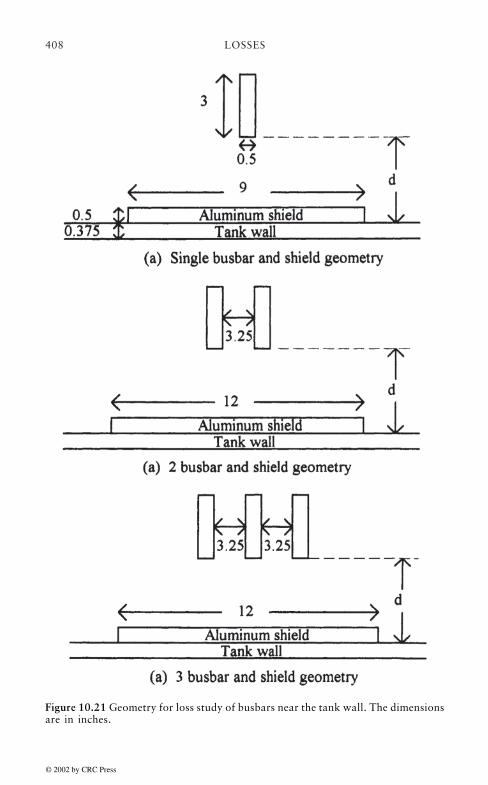
LOSSES408
Figure 10.21 Geometry for loss study of busbars near the tank wall. The dimensionsare in inches.
© 2002 by CRC Press

LOSSES 409
Since the busbars were modeled as solid copper and have a fairlylarge cross-sectional area, there were extra losses induced in thembeyond the usual I2R losses based on d.c, resistance. We found that theseextra eddy current losses amounted to about 20% of the I2R losses,regardless of whether one or groups of 2 or 3 busbars were studied. Inthe following figures, we plot the normalized losses which should bemultiplied by the total length of the busbars or busbar group and by thecurrent in kA squared to get the total loss, not including the loss in thebusbars themselves. Thus the loss plotted is the tank loss when noshields are present and the tank plus shield loss when a shield is present.
Fig. 10.22 shows the normalized loss versus distance, with andwithout shield for the single busbar case. The figure shows that thelosses without shield drop off with distance, d, while the losses withshield are relatively constant with distance. In the shielded case, therelative amounts of loss in the shield and tank wall change withdistance, while their sum, which is plotted, remains almost constant.We see that shielding reduces the losses by about a factor of 5 at closedistances and a factor of 2–3 at further distances compared with theunshielded losses.
Fig. 10.23 shows the normalized losses versus distance for the twobusbar case. This figure has nearly the same features as the singlebusbar case. In fact, even the magnitude of the losses is nearly the same.However, since this figure applies to 2 busbars, this says that the lossescan be cut in half by pairing 2 phases compared with leaving themseparate. We also see in this case that shielding is very effective inreducing the losses.
Fig. 10.24 shows the normalized loss versus distance for a group of 3busbars. We see that the magnitude of the loss is considerably reducedrelative to the single or double busbar case. In fact, the losses shownshould be divided by 3 to compare with the single busbar loss. In thiscase, shielding does not provide much improvement. This is because the3 phase currents sum to zero at any instant of time, producing little netmagnetic field at distances large relative to the conductor spacings. Fig10.25 shows a flux plot of the 3 busbar case, where the flux cancellationcan be directly observed.
It thus appears that loss reduction from busbars near bare tank wallscan be achieved by pairing 2 or 3 phases together, the latter beingpreferable. Shielding is very effective in reducing the losses associatedwith 1 or 2 busbars from different phases but not for 3 busbars where thelosses are small anyway.
© 2002 by CRC Press

LOSSES410
Figure 10.22 Stray losses due to a single busbar running parallel to the tank wall.The geometry is shown in Fig. 10.21a.
Figure 10.23 Stray losses due to two side by side busbars from different phasesand running parallel to the tank wall. The geometry is shown in Fig. 10.21b.
© 2002 by CRC Press

LOSSES 411
Figure 10.24 Stray losses due to a group of 3 busbars from different phases of athree phase system and running parallel to the tank wall. The geometry is shownin Fig. 10.21c.
Figure 10.25 Flux plot from a balanced 3 phase set of busbars near tank wallwith shield.
© 2002 by CRC Press

LOSSES412
10.3.2.6 Tank Losses Associated with the Bushings
Current enters and leaves a transformer tank via the bushings. Thebushings are designed to handle the voltage stresses associated with thevoltage on the leads without breakdown as well as to dissipate heat dueto the losses in the conductor which passes through the bushings. Theconductor or lead, which must pass through the tank wall, creates amagnetic field which can generate eddy currents and accompanyinglosses in the tank wall near the lead. These losses must be calculatedand appropriate steps taken to reduce them if necessary.
We can obtain a reasonable estimate of the tank losses due to a leadpenetrating the tank wall by resorting to an idealized geometry asshown in Fig. 10.26. Thus we assume an infinitely long circular cross-section lead passing perpendicularly through the center of a circularhole in the tank wall. We can assume that the tank wall itself is a circleof large radius centered on the hole. Since the losses are expected toconcentrate near the hole, the actual radial extent of the tank won’tmatter much. Also since most of the magnetic field which generateseddy currents in the tank comes from the portion of the lead near thetank, the infinite extent of the lead does not greatly affect thecalculation.
The geometry in Fig. 10.26 is axisymmetric. Thus we need to workwith Maxwell’s equations in a cylindrical coordinate system. Weassume the tank wall has permeability µ and conductivity σ.Combining Maxwell’s equations with Ohm’s law inside the tank walland assuming that H varies harmonically in time as
H(r, t)=H(r)ejωt (10.49)
we get
(10.50)
where H in (10.50) is only a function of position.
© 2002 by CRC Press

LOSSES 413
Because the problem is axisymmetric, H does not depend on ϕ, theazimuthal angle. We also assume that H has only a component. This isall that is needed to produce the expected eddy current pattern indicatedin Fig. 10.26b, where the eddy currents approach and leave the holeradially and the paths are completed along short sections in the z-direction. The approximate solution we develop here will neglect thesez-directed eddy currents which should not contribute much to the totalloss. Thus we have
H(r)=Hϕ(r, z)aϕ (10.51)
where aϕ is the unit vector in the azimuthal direction. Expressing (10.50)in cylindrical coordinates and using (10.51), we get
Figure 10.26 Idealized geometry and parameters used to calculate losses due toa lead passing through the tank
© 2002 by CRC Press

LOSSES414
(10.52)
We need to solve this equation subject to the boundary conditions
(10.53)
where a is the radius of the hole in the tank wall and c is the tank wallthickness. Once a solution is found, the current density J is given by
(10.54)
where r and k are unit vectors in the r and z directions.To solve (10.52), we use a separation of variables technique and
write
Hϕ(r, z)=R(r)Z(z) (10.55)
Substituting into (10.52) and dividing by RZ, we obtain
(10.56)
Thus we have two terms which are separately a function of r and z andwhose sum is a constant. Hence, each term can be separately equated toa constant so long as their sum is jωµσ. We choose
(10.57)
Letting k2=jωµσ so that
© 2002 by CRC Press

LOSSES 415
(10.58)
we can solve the first equation in (10.57) up to an overall multiplicativeconstant, Zo,
Z(z)=Zo cosh(kz)=Zo[cosh(qz)cos(qz)+jsinh(qz)sin(qz)] (10.59)
This equation takes into account the symmetry about the z=0 plane.The second equation in (10.57) is solved up to an overall multiplicativeconstant, Ro, by
(10.60)
Thus the complete solution to (10.56), using the boundary conditions(10.53) is
(10.61)
This does not exactly satisfy the first boundary condition in (10.53)except in the limit of small qc/2.
Solving for the eddy currents, equation (10.54), we see that the z-directed currents are zero when we substitute the solution (10.61). Weexpect that the losses contributed by these short paths will be small.Solving for the r-directed eddy currents, we obtain
(10.62)
and the loss density as a function of position, assuming I is an rmscurrent, is
(10.63)
© 2002 by CRC Press
LOSSES416
This drops off with radius as 1/r2 and so is highest near the opening. Thetotal loss is given by
(10.64)
The upper limit of the r integration, b, is chosen to be a large enoughradius that the tank area of interest is covered. The result will not be toosensitive to the exact value chosen. Performing the integrations in (10.64),we obtain
(10.65)
For a magnetic steel tank wall, using µr=200, σ=4×10⁶ (Ω-m)-1, f=60 Hz,c=9.52×10⁻³ m (0.375 in), we have qc=4.15 as was found previously.Thus the small qc approximation to (10.65) cannot be used. Howeverfor a stainless steel tank wall of the same thickness and frequency, usingµr=1, µ=4π×10-7 H/m, σ=1.33×10⁶ (Ω-m)-1, we have qc=0.17 so the lowqc limit of (10.65) may be used. This is
(10.66)
where ω=2πf and σ=1/ρ have been substituted. Applying these last twoequations to the case where I=1000 Amps rms (for normalizationpurposes), the hole radius a=0.165 m (6.5 in), the outer radius b=0.91 m(36 in), and using the above parameters for the two types of steel, we getLossbush(mag steel)=61.9 Watts/(kArms)2 and Lossbush(stainless) =5.87×10⁻³
Watts/(kArms)2. These losses are associated with each bushing. Applyingthis to a situation where the lead is carrying 10 kArms, the loss in amagnetic steel tank wall would be 6190 Watts per bushing and in astainless steel tank wall 0.587 Watts per bushing. These need to bemultiplied by the number of bushings carrying the given current to getthe total tank loss associated with the bushings. Thus when heavy currentsare carried by the leads, it might be worth while to insert a stainlesssteel section of tank around the bushings, especially since these lossesare concentrated in the part of the tank wall near the opening.
© 2002 by CRC Press
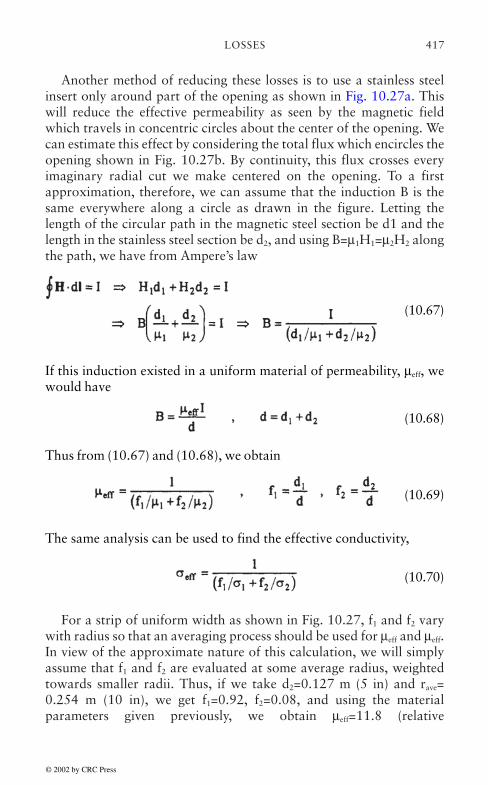
LOSSES 417
Another method of reducing these losses is to use a stainless steelinsert only around part of the opening as shown in Fig. 10.27a. Thiswill reduce the effective permeability as seen by the magnetic fieldwhich travels in concentric circles about the center of the opening. Wecan estimate this effect by considering the total flux which encircles theopening shown in Fig. 10.27b. By continuity, this flux crosses everyimaginary radial cut we make centered on the opening. To a firstapproximation, therefore, we can assume that the induction B is thesame everywhere along a circle as drawn in the figure. Letting thelength of the circular path in the magnetic steel section be d1 and thelength in the stainless steel section be d2, and using B=µ1H1=µ2H2 alongthe path, we have from Ampere’s law
(10.67)
If this induction existed in a uniform material of permeability, µeff, wewould have
(10.68)
Thus from (10.67) and (10.68), we obtain
(10.69)
The same analysis can be used to find the effective conductivity,
(10.70)
For a strip of uniform width as shown in Fig. 10.27, f1 and f2 varywith radius so that an averaging process should be used for µeff and µeff.In view of the approximate nature of this calculation, we will simplyassume that f1 and f2 are evaluated at some average radius, weightedtowards smaller radii. Thus, if we take d2=0.127 m (5 in) and rave=0.254 m (10 in), we get f1=0.92, f2=0.08, and using the materialparameters given previously, we obtain µeff=11.8 (relative
© 2002 by CRC Press

LOSSES418
permeability) and σeff=3.45×10⁶ (Ω-m)”1. Using these parameters, we getqc=0.935 so that, from (10.65) we obtain Lossbush=2.05 Watts/(kArms)2
for a single bushing. This is a considerable reduction from the losswithout a stainless steel insert. At a current of 10 kArms, this is a loss of205 Watts per bushing.
Figure 10.27 Openings for three phase leads in the tank wall with stainless steelstrips inserted to reduce the permeability
10.3.3 Winding Losses Due to Missing or Unbalanced Cross-Overs
When two or more wires or cables in parallel are used to construct awinding, it is necessary to interchange their positions at suitable pointsalong the winding in order to cancel out induced voltages produced bythe stray flux. Otherwise, any net induced voltage can drive currentsaround the loop established when the parallel turns are joined at eitherend of the winding and these circulating currents will produce extralosses. The interchange points are called cross-overs and their numberwill depend on the number of parallel strands and on the symmetry ofthe stray flux pattern. An extreme example of cross-overs is provided bytransposed cable where cross-overs occur among the individual strands
© 2002 by CRC Press

LOSSES 419
comprising the cable at relatively short equally spaced intervals alongthe cable. Thus a single cable can be wound into a coil without anyneed for additional cross-overs within the cable.
In order to estimate the losses associated with missing or unbalancedtranspositions, we make some simplifying assumptions. We assume thatthe windings are uniformly wound and that the magnetic field pattern isas shown in Fig. 10.28 for an inner and outer winding. Thus we areignoring end effects. Although this assumption is reasonably accuratefor coils long compared with their radii, it loses some accuracy for shortcoils or coil sections. However, it should be clear in the followingdevelopment where improvements can be made for more accuracy.
Figure 10.28 Idealized magnetic field pattern for an inner-outer winding pair.The parameters h and d can differ for the two windings.
© 2002 by CRC Press

LOSSES420
Since the permeability in the coil region is close to the permeabilityof vacuum or air, µo, we have for the B field of an inner coil, Bin, or outercoil, Bout, in SI units,
(10.71)
where h is the coil height, d its radial build, N the total number ofelectrical turns in the winding, I the current, and x the distance throughthe radial build, starting at the inner radius. These parameters can differfor the inner and outer coils.
We assume that there are n radial turns in parallel. Any axial turnsin parallel do not see a different flux pattern from their radialcounterpart to first order. It is therefore unnecessary to consider them incalculating voltage imbalances. The voltage induced in the ith parallelradial turn by the leakage flux is different from that seen by the jth fori≠j. Therefore it is necessary to interchange parallel radial turns so thateach one occupies the position of all the others as the winding proceedsalong the coil axis. If an interchange is missing or misplaced, differentvoltages will be induced in the parallel turns and the voltage differenceswill drive circulating currents around the loops formed by the top andbottom connections.
Let us calculate the voltage induced in a single turn in the ith
position. This will equal the time derivative of the flux linkage, λi.Referring to Fig. 10.29, the flux linkage for the ith turn is
(10.72)
Here Bin or Bout should be substituted for B to obtain λi,in or λi,out for innerand outer coils. t is the turn radial thickness and d=nt. ro is the innerradius of the coil. In the first term above, the integration is up to theinner radius of the turn so all the flux is linked by the whole turn. In thesecond term, the flux linkage changes from 1 at the start of the integralto 0 at the end and this is taken care of by the factor (i”x/t). For Bout weare ignoring the flux for radii <ro. This is the same for all the turns andwill not contribute to voltage differences between parallel radial turns.
© 2002 by CRC Press

LOSSES 421
Substituting (10.71) into (10.72) and integrating, we obtain
(10.73)
These are the flux linkages per turn. If there are Nu uncompensatedelectrical turns due to missed or unbalanced cross-overs, then (10.73)should be multiplied by Nu to get the total flux linkage corresponding toparallel radial turn i. Assuming sinusoidal currents of angular frequencyω=2πf, we obtain for the induced voltages,
(10.74)
The number of unbalanced electrical turns needs to be estimated foreach particular case. For instance, if there are n parallel radial turns,there should be a minimum of n-1 equally spaced cross-overs, assuming
Figure 10.29 Radial parallel turn numbering scheme and geometric parametersfor determining induced voltages
© 2002 by CRC Press
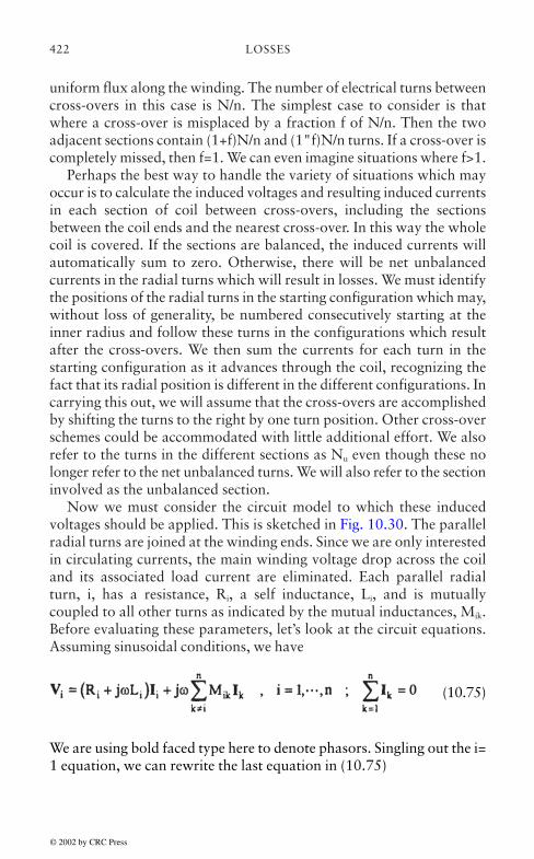
LOSSES422
uniform flux along the winding. The number of electrical turns betweencross-overs in this case is N/n. The simplest case to consider is thatwhere a cross-over is misplaced by a fraction f of N/n. Then the twoadjacent sections contain (1+f)N/n and (1"f)N/n turns. If a cross-over iscompletely missed, then f=1. We can even imagine situations where f>1.
Perhaps the best way to handle the variety of situations which mayoccur is to calculate the induced voltages and resulting induced currentsin each section of coil between cross-overs, including the sectionsbetween the coil ends and the nearest cross-over. In this way the wholecoil is covered. If the sections are balanced, the induced currents willautomatically sum to zero. Otherwise, there will be net unbalancedcurrents in the radial turns which will result in losses. We must identifythe positions of the radial turns in the starting configuration which may,without loss of generality, be numbered consecutively starting at theinner radius and follow these turns in the configurations which resultafter the cross-overs. We then sum the currents for each turn in thestarting configuration as it advances through the coil, recognizing thefact that its radial position is different in the different configurations. Incarrying this out, we will assume that the cross-overs are accomplishedby shifting the turns to the right by one turn position. Other cross-overschemes could be accommodated with little additional effort. We alsorefer to the turns in the different sections as Nu even though these nolonger refer to the net unbalanced turns. We will also refer to the sectioninvolved as the unbalanced section.
Now we must consider the circuit model to which these inducedvoltages should be applied. This is sketched in Fig. 10.30. The parallelradial turns are joined at the winding ends. Since we are only interestedin circulating currents, the main winding voltage drop across the coiland its associated load current are eliminated. Each parallel radialturn, i, has a resistance, Ri, a self inductance, Li, and is mutuallycoupled to all other turns as indicated by the mutual inductances, Mik.Before evaluating these parameters, let’s look at the circuit equations.Assuming sinusoidal conditions, we have
(10.75)
We are using bold faced type here to denote phasors. Singling out the i=1 equation, we can rewrite the last equation in (10.75)
© 2002 by CRC Press
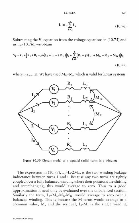
LOSSES 423
(10.76)
Subtracting the V1 equation from the voltage equations in (10.75) andusing (10.76), we obtain
(10.77)
where i=2,…, n. We have used Mik=Mki which is valid for linear systems.
The expression in (10.77), L1+Li-2M1i, is the two winding leakageinductance between turns 1 and i. Because any two turns are tightlycoupled over a fully balanced winding where their positions are shiftingand interchanging, this would average to zero. Thus to a goodapproximation it need only be evaluated over the unbalanced section.Similarly the term, L1+Mik-M1i-M1k, would average to zero over abalanced winding. This is because the M terms would average to acommon value, M, and the residual, L1-M, is the single winding
Figure 10.30 Circuit model of n parallel radial turns in a winding
© 2002 by CRC Press

LOSSES424
leakage impedance between turn 1 and any other turn and it willaverage to zero because of the close coupling of the turns. Therefore,this expression need only be evaluated over the unbalanced section.However, the resistances in (10.77) must be evaluated over the fulllength of the winding since they do not depend on the turn coupling.This will have nearly the same value for all the turns.
In order to evaluate the self and mutual inductances in the circuitmodel, we will assume that the unbalanced section is long enoughaxially that the same approximations as were used for the inducedvoltage calculation are also valid here. Thus the magnetic field for acoil of Nu turns located at the ith radial position is shown in Fig. 10.31.Analytically, the B-field is
(10.78)
where hu is the axial height of the unbalanced section (=h Nu/N).
The flux linkage to itself, λii, is
Figure 10.31 Magnetic field for a coil consisting of Nu turns at radial position i
(10.79)
© 2002 by CRC Press

LOSSES 425
The turn linkage factor Nu(1-x/t) has been included in the second term.Performing the integral, we obtain
(10.80)
From this, the self inductance, Li, is
(10.81)
so that
(10.82)
The mutual inductance between turns i and k can be found, againusing Fig. 10.31 and (10.78). Let turn k be outside of turn i. Then theflux linked to turn k from flux produced by turn i, λik, is
(10.83)
so that the mutual inductance is
(10.84)
This same expression would have been obtained if k were the coil creatingthe magnetic field. Thus in (10.84), the terms involving i on the righthand side refer to the inner winding of the pair. This insures that Mik=Mki.From (10.84), we obtain
© 2002 by CRC Press

LOSSES426
(10.85)
since 1 is always the inner winding in the unbalanced section.Using these formulas, we find for the two winding leakage
impedance term in (10.77),
(10.86)
This formula holds for i>1. This same expression could have beenobtained by energy methods. The second expression in (10.77) can alsobe obtained from the above formulas,
(10.87)
This last formula holds for i<k and i, k>1. If i>k, substitute k for i on theright hand side.
The resistances, Ri and R1 in (10.77) are roughly the same for allturns. In the standard formula R=ρ/A, is the length of a parallelradial turn over the whole winding and A is its cross sectional area,including the area of any corresponding axially displaced turns inparallel with it.
Let us cast (10.77) in matrix form by defining a matrix X withelements
(10.88)
i.e. we are renumbering the equations so that they start from 1 ratherthan 2. Similarly, define a resistance matrix R,
© 2002 by CRC Press

LOSSES 427
(10.89)
Let us also define a vector of voltages, E, and currents, K, by
(10.90)
Here bold faced type is doing dual service in distinguishing vectorsand phasors. Then we can write (10.77) in matrix form
E=(R+jX)K (10.91)
Separating E and K into real and imaginary parts,
(10.92)
we can write (10.91) as a real matrix equation
(10.93)
where the elements in this equation are vectors or matrices. From (10.74),we see that the voltages depend on the main coil current which can betaken to be real so we can set EIm=0.
These equations are solved for the complex currents Ki=Ii+1 and thenI1 is given by(10.76). These currents apply to the standard ordering, 1,…, n. Thesesame equations, with different Nu and hu are solved for the otherconfigurations making up the winding and the currents correspondingto the position of turn i in each configuration are added for i=1,…, n.Thus we obtain
(10.94)
Here bold faced type indicates phasor quantities. Once these currentsare obtained, the losses are found from
© 2002 by CRC Press

LOSSES428
(10.95)
As a numerical example, we solved an inner coil problem with across-over shifted by 4 electrical turns and with the followingparameters:
ro=0.567 m (22.3 in)h=2.60 m (102.5 in)d=8.25 cm (3.25 in)t=2.06 cm (0.813 in)N=80n=4Nu=4N/n=20A=Resistance area=3.71 cm2 (0.575 in2)I=6449 Ampsρ=2×10⁻⁸ Ω-m
We obtained for the losses due to circulating currents 12.3 kW. Thisshould be compared with the total I2R losses of 171 kW. Thus thecirculating current loss amounts to about 7% of the I2R loss in this case,
The above calculation could be improved by using more accurateexpressions for the inductances and mutual inductances, reflecting thefact that the unbalanced sections are not necessarily axially very long.
© 2002 by CRC Press

429
11. THERMAL MODEL OF A COREFORM POWER TRANSFORMER ANDRELATED THERMAL CALCULATIONS
Summary A model of a core form power transformer is presented whichutilizes a detailed network of oil flow paths through the coils andradiators. Along each path segment, oil velocities, temperatures, andtemperature rises are computed. The oil flows may be either thermallyor pump driven. Throughout the disk coils, the flow is assumed directedby means of oil flow washers. Temperatures are computed for each diskalong the disk coils. Coils with non-directed oil flow are also treated butin less detail. The model includes temperature dependent oil viscosity,resistivity, and oil density as well as both temperature and velocitydependent heat transfer and friction coefficients. The resulting non-linearsystem of equations is solved iteratively. The radiator oil flow is alsotreated by means of a similar network model. Radiator cooling can beby natural convection or fans. Tank cooling by convection and radiationis also included. Iterations are performed in a back and forth mannerbetween the coils and radiators until steady state is reached where theelectric power losses equal the losses to the surroundings. Someassumptions regarding the temperature distribution of the tank oil andtank oil flows are made in order to tie the coil and radiator flows together.Although detailed output information is available such as pathtemperatures and velocities, average coil, coil hot spot, average oil,and top oil temperatures are also computed and compared with testdata. In the transient version, time constants and times at overload untila particular hot spot or top oil temperature is reached can be obtained.Other thermal issues such as the loss of life determination, cable, tieplate,and tank wall temperatures are also addressed.
11.1 INTRODUCTION
A thermal model of an oil cooled power transformer is presented here,along with details of the computer implementation and experimentalverification. Any such model, particularly of such a complex system, isnecessarily approximate. Thus, the model assumes that the oil flows indefinite paths and ignores local circulation or eddy patterns which may
© 2002 by CRC Press
THERMAL MODEL430
arise. Since we assume that the oil flow through the disk coils is guidedby means of oil flow washers, this assumption should be fairly accuratefor these types of coils. Although recent studies have shown that irregulareddy flow patterns may exist in non-directed oil flow cooling in verticalducts [Pie92], these types of coils occur to a very limited extent in ourdesigns. Such patterns may also occur in the bulk tank oil. We assumethese are small compared with the major or average convective coolingflow in the tank. We further assume that the convective flow in the tankresults in a linear temperature profile from the bottom of the radiatorsto the top of the coils in the tank oil external to the coils. The modellikewise ignores localized heating which may occur, for example, dueto high current carrying leads near the tank wall. It accounts for thesetypes of stray losses in only an average way. However, a localizeddistribution of eddy current losses in the coils is allowed for, along withthe normal I2R losses.
The radiators we model consist of a collection of radiator platesspaced equally along inlet and outlet pipes. The plates contain severalvertical ducts in parallel. The ducts have oblong shaped, nearlyrectangular, cross-sections. Fans, vertically mounted, may or may not bepresent (or turned on). In addition to radiator cooling, cooling also occursfrom the tank walls by both natural convection to the surrounding air andby radiation. Although the oil may be pumped through the radiators,most of our designs are without pumps so that the oil flow in the radiatorsand coils is laminar. This determines the expressions used for the heattransfer and friction coefficients along the oil flow paths.
Our model of a disk winding is similar to that of Oliver [Oli80].However, since we consider the whole transformer, we need to reconcilethe oil flows and heat generated by the individual coils plus stray losseswith the radiator and tank cooling in an overall iteration scheme in orderto arrive at a steady state condition. We also consider transient heating.
Previous thermal models of whole transformers have focused ondeveloping analytic formulas with adjustable parameters to predictoverall temperature rises of the oil and coils [IEE81, Blu51, Eas65,Tay58, Aub92, Pie92a]. While these produce acceptable results onaverage or for a standard design, they are less reliable whenconfronting a new or untried design. The approach taken here is todevelop a model to describe the basic physical processes occurring inthe unit so that reliance on parameter fitting is minimized. Such anapproach can accommodate future improvements in terms of a moredetailed description of the basic processes or the addition of newfeatures as a result of a design change.
© 2002 by CRC Press

431THERMAL MODEL
11.2 THERMAL MODEL OF A DISK COIL WITH DIRECTED OILFLOW
This section is essentially a reprint of our published paper [Del99]. ©1999 IEEE. Reprinted, with permission, from the Proceedings of the1999 IEEE Transmission and Distribution Conference, New Orleans,LA, 11–16 April, 1999, pp. 914–919.
The disk coil is assumed to be subdivided into directed oil flowcooling paths as shown in Fig. 11.1. We number the disks, nodes, andpaths, using the scheme shown. The geometry is really cylindrical andthe inner radius Rin is indicated. Only one section (region between twooil flow washers) and part of a second is shown, but there can be asmany sections as desired. Each section can contain different numbers ofdisks and the number of turns per disk, insulation thickness, etc. canvary from section to section. The duct sizes can vary within a section aswell as from section to section.
Figure 11.1 Disk, node, and path numbering scheme for a disk coil with directed oilflow
© 2002 by CRC Press

THERMAL MODEL432
In Fig. 11.3 we have indicated the unknowns which must be solvedfor at each node and path. These include the nodal temperatures, T, thenodal pressures, P, the path oil velocities, v, the path oil temperaturerises, ∆T, and the disk temperatures, TC. These are labeled with theircorresponding node, path or disk number. Note that we are notallowing for a temperature profile along a single disk but are assumingthat each disk is at a uniform temperature. This is an approximationwhich could be refined if more detail is required.
Fig. 11.2 shows the cross-sectional areas, A, and hydraulicdiameters, D, of the various paths. Normally the vertical ductgeometric parameters, labeled 1 and 2, are the same throughout the coilbut the horizontal duct values can differ along the coil.
Figure 11.2 Cross-sectional areas and hydraulic diameters of different oil paths. Thevertical ducts are assumed to be uniform along the coil.
© 2002 by CRC Press

433THERMAL MODEL
11.2.1 Oil Pressures and Velocities
Along a given path, the oil velocities are uniform since the cross-sectionalarea is assumed to remain constant. Ignoring gravitational effects, thepressure drop along a given path is only required to overcome frictionTreating a generic path and labeling the pressures at the beginning andend of the path P1 and P2 respectively, we can write, using standardnotation [Dai73],
(11.1)
where ρ is the fluid density, f the friction coefficient, L the path length, Dthe hydraulic diameter, and v the fluid velocity. We note that the hydraulicdiameter is given by
Figure 11.3 Numbering scheme for disk temperatures, node temperatures, nodepressures, path velocities, and path temperature changes. Also indicated are the heattransfer surface areas, Ac, and the heat transfer coefficients, h, for these surfaces.
© 2002 by CRC Press

THERMAL MODEL434
D=4×cross-sectional area/wetted perimeter
MKS units are used throughout this report. For laminar flow in circularducts, f=64/ReD,
where ReD is the Reynolds number, given by
(11.2)
where µ is the fluid viscosity. For laminar flow in non-circular ducts,the number 64 in the expression for f changes. In particular, forrectangular ducts with sides a and b with a<b, we can write
(11.3)
where K(a/b) is given approximately by
K(a/b)=56.91+40.31(e-3.5a/b-0.0302) (11.4)
This expression is based on a fit to a table given in reference [Ols80].Substituting (11.2) and (11.3) into (11.1), we obtain
(11.5)
where K=K(a/b) is implied. This equation is linear in the pressures andvelocities. However, the oil viscosity is temperature dependent and thiswill necessitate an iterative solution. Based on a table of transformer oilviscosities verses temperature given in [Kre80], we achieved a good fitto the table with the expression
(11.6)
with T in °C and µ in Ns/m2.For non-laminar flow (ReD>2000), the expression for f is more
complicated and (11.5) would no longer be linear in v. Note that we areignoring the extra friction arising from flow branching and directionchanging at the nodes. There is considerable uncertainty in the
© 2002 by CRC Press

435THERMAL MODEL
literature as to what these additional factional effects are for laminarflow. Instead we have chosen to allow the friction coefficient in (11.3) tobe multiplied by a correction factor which is the same for all thebranches. This correction factor is close to 1 in practice for disk coils.
We get an equation of type (11.5) for all the paths in Fig. 11.1. Notethat we need only solve for the unknowns in one section at a time sincethe values at the topmost node and path can be taken as input to thenext section. There are 3n+2 paths in the section, where n is the numberof disks. However, the number of pressure unknowns is 2n+2, i.e. thenumber of nodes. We do not include the node 0, where the pressure mustbe input. This pressure will be given by the requirement that the overallpressure drop through the coil is determined by buoyancy effects as willbe discussed below. The number of velocity unknowns is 3n+2 or thenumber of paths. Hence 2n+2 additional equations are required to solvefor the pressures and oil velocities. We will treat the temperatures asfixed during the solution process. A separate set of equations will bederived for the temperatures and the two systems will ultimately becoupled through back and forth iteration.
The additional equations needed to solve for the pressures andvelocity unknowns come from conservation of mass at the nodes. Themass of fluid of velocity v flowing through a duct of cross-sectional areaA per unit time, dM/dt, is given by
(11.7)
Since the fluid is nearly incompressible, we can consider conservationof volume instead, where Q=Av is the volume flow per unit time. Referringto Fig. 11.3 and using the areas indicated in Fig. 11.2, we obtain for atypical inner (smallest radii) node, 2i-1,
A1v3i-2=A1v3i+1+Ao,iv3i-1 (11.8)
and for a typical outer node, 2i,
Ao,iv3i-1+A2v3i-3=A2v3-i (11.9)
However, the nodes at the beginning and end require special treatment(see Fig. 11.1). We want to calculate the velocity on path 3n+3 which isinput to the next coil. We assume that the input velocity at the bottom of
© 2002 by CRC Press

THERMAL MODEL436
the section, v1 on path 1, is known by some other means (overall energybalance). This still leaves 3n+2 unknown velocities to solve for but v3n+3
will be re-labeled v1 and v1 will be called vo, a known input velocity.Thus at node 1 we have
A1vo=A1v4+Ao,1v2 (11.10)
At node 2,
Ao,1v2=A2v3 (11.11)
At node 2n+1
A1v3n+1=Ao,n+1v3n+2 (11.12)
and at node 2n+2
Ao,n+1 v3n+2+A2v3n=A2v1 (11.13)
We have 5n+4 equations to solve for the pressure and velocityunknowns, where n is the number of disks in the section. For n=30,which is about as large a number of disks as would be used in onesection, this yields 154 equations. Since the equations are quite sparse,a linear equation solver which uses sparsity techniques was used. Notethat the cross-sectional areas must be calculated taking into account thearea lost due to key spacers or vertical spacer sticks. These alsoinfluence the hydraulic diameters.
The overall pressure drop through the coil is produced by thedifference in buoyancy between the hot oil inside the coil’s cooling ductsand the cooler tank oil outside the coil. Thus
∆Pcoil=(ρave,out-ρave,in)gH (11.14)
where ρave,in is the average oil density inside the coil and ρave,out theaverage density immediately outside the coil, g is the acceleration ofgravity, and H the coil height. Letting β be the volume coefficient ofthermal expansion, we have
(11.15)
© 2002 by CRC Press

437THERMAL MODEL
and thus, since β=6.8×10⁻⁴/°K for transformer oil, we have to a goodapproximation over a reasonably large temperature range, ∆ρ=βρ∆Tso that (11.14) can be written
∆Pcoil=βρgH(Tave,in-Tave,out) (11.16)
Because we are only considering pressures which produce oil flows, thepressure at the top of the coil when steady state is achieved should bezero. This means that ∆Pcoil=Po, the pressure at node 0 in Fig. 11.1.
The oil velocity into the coil along path 1 is determined by theoverall energy balance. The energy per unit time acquired by the oilmust equal the energy per unit time lost by the coil. In steady state, thelatter is just the total resistive loss of the coil. Thus
(11.17)
where c is the specific heat of the oil, ∆Toil is the increase in temperatureof the oil after passing through the coil, and Ri is the temperaturedependent resistance of disk i, including eddy current effects. We use
Ri=γo(1+α∆Ti)(1+ecfi)i/Aturn (11.18)
where γo is the resistivity at some standard temperature, Tstd, ∆Ti is thetemperature rise of the disk above the standard temperature, α thetemperature coefficient of resistivity, ecfi the fraction of the normal lossesdue to eddy currents for disk i, i the length of the cable or wire in diski, and Aturn the cross-sectional current-carrying area of the cable or wire.Note that ecfi can vary from disk to disk to account for the effects ofnon-uniform stray flux along the coil. For a given temperaturedistribution for the disks and for known input and output oil temperatures,(11.17) can be solved for v0. These temperatures will be given by asubsequent analysis and a back and forth iteration is required to achieveconsistency. Using these results, the path 1 equation can be written
(11.19)
which contains only P1 as an unknown.
© 2002 by CRC Press
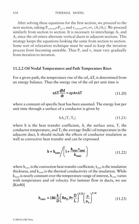
THERMAL MODEL438
After solving these equations for the first section, we proceed to thenext section, taking Po,second=P2n+2 and vo,second=v1=vo (A1/A2). We proceedsimilarly from section to section. It is necessary to interchange A1 andA2 since the oil enters alternate vertical ducts in adjacent sections. Thisstrategy keeps the equations looking the same from section to section.Some sort of relaxation technique must be used to keep the iterationprocess from becoming unstable. Thus Po and vo must vary graduallyfrom iteration to iteration.
11.2.2 Oil Nodal Temperatures and Path Temperature Rises
For a given path, the temperature rise of the oil, ∆T, is determined froman energy balance. Thus the energy rise of the oil per unit time is
(11.20)
where a constant oil specific heat has been assumed. The energy lost perunit time through a surface of a conductor is given by
hAc(Tc-Tb) (11.21)
where h is the heat transfer coefficient, Ac the surface area, Tc theconductor temperature, and Tb the average (bulk) oil temperature in theadjacent duct, h should include the effects of conductor insulation aswell as convective heat transfer and can be expressed
(11.22)
where hconv is the convection heat transfer coefficient, τinsul is the insulationthickness, and kinsul is the thermal conductivity of the insulation. Whilekinsul is nearly constant over the temperature range of interest, hconv varieswith temperature and oil velocity. For laminar flow in ducts, we use[Kre80]
(11.23)
© 2002 by CRC Press

439THERMAL MODEL
where k is the thermal conductivity of the oil, D the hydraulic diameter,L the duct length, ReD the Reynolds number (11.2), Pr the Prandtl number(Pr=µc/k), the viscosity of the bulk oil, and µs the oil viscosity at theconductor surface. Equation (11.23) applies when ReD Pr D/L>10. Acorrection must be applied for smaller values. The major temperaturevariation comes from the viscosity (11.6) and the velocity dependencecomes from the Reynold’s number. The other parameters are nearlyconstant over the temperatures of interest. For transformer oil, we use[Kre80] ρ=867 kg/m3, c=1880 J/kg°C, k=0.11 W/m°C.
Equating energy gains and losses per unit time (equations (11.20)and (11.21)), we have for a horizontal duct between 2 disks (path 3i-1 inFig. 11.3)
cρAo,iv3i-1∆T3i-1=h3i-1Ac,o[(Tc,i-Tb,3i-1)+(Tc,i-1-Tb,3i-1)] (11.24)
where losses occur through 2 conductor surfaces and the bulk duct oiltemperature, Tb,3i-1, is approximately given by
Tb,3i–1=T2i–1+∆T3i–1/2 (11.25)
with T2i-1 the nodal oil temperature at the duct’s entrance. For horizontalducts at the beginning and end of a section, only one conductor surfacecontributes to the right side of (11.24). For the vertical ducts, we have
(11.26)
for the left and right ducts 3i+1 and 3i respectively. We obtain 3n+2equations in this manner. However, along the entrance and exit ducts(ducts 1 and 3n+3) we have ∆T=0 since no heat is going into the oilhere. Hence this equation and unknown can be eliminated.
We obtain further equations from energy balance at the nodes. Thusthe thermal energy which the oil carries into a node must equal thatleaving. The thermal energy per unit time carried by a mass of oilmoving with velocity v normal to a surface of area A is given by
© 2002 by CRC Press

THERMAL MODEL440
ρcAv(T-Tref) (11.27)
assuming c remains constant from some reference temperature Tref up tothe temperature of interest T. Balancing these energy flows at node 2i-1in Fig. 11.3, we obtain
Canceling ρc and using (11.8) we get
T2i-3+∆T3i-2=T2i-1 (11.28)
Similarly at node 2i we obtain,
Ao,iV3i-1(T2i-1+∆T3i-1)+A2v3i-3(T2i-2+∆T3i-3)=A2 v3iT2i (11.29)
These equations are slightly modified for a few nodes at the beginningand end of a section, as was done for the mass conservation equations.
The temperature at node 0 or 1 will be taken as an input. It is thebottom tank oil temperature and will be obtained from an overallbalance of heat generation and loss. The calculated temperature at thetopmost node of the section, 2n+2, will be taken as input to the nextsection so that the calculation can proceed section by section up the coilas was the case for the pressure-velocity equations. The temperaturedependence of the heat transfer coefficients makes these equations non-linear. In addition, this coefficient depends on the oil velocity whichrequires iteration between these equations and the pressure-velocityequations. Another set of unknowns which appear in these equations arethe disk temperatures Tc. These have not been dealt with yet. They areprobably best solved for separately.
11.2.3 Disk Temperatures
The disk temperatures can be found by equating the I2R losses to theheat passing through the disk surface in the steady state. Thus, for thegeneric disk shown in Fig. 11.3, we have, using previously definedparameters,
© 2002 by CRC Press
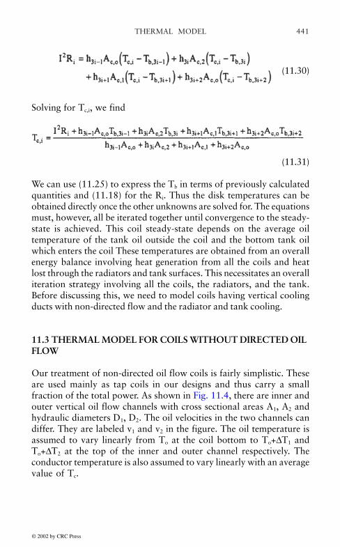
441THERMAL MODEL
(11.30)
Solving for Tc,i, we find
(11.31)
We can use (11.25) to express the Tb in terms of previously calculatedquantities and (11.18) for the Ri. Thus the disk temperatures can beobtained directly once the other unknowns are solved for. The equationsmust, however, all be iterated together until convergence to the steady-state is achieved. This coil steady-state depends on the average oiltemperature of the tank oil outside the coil and the bottom tank oilwhich enters the coil These temperatures are obtained from an overallenergy balance involving heat generation from all the coils and heatlost through the radiators and tank surfaces. This necessitates an overalliteration strategy involving all the coils, the radiators, and the tank.Before discussing this, we need to model coils having vertical coolingducts with non-directed flow and the radiator and tank cooling.
11.3 THERMAL MODEL FOR COILS WITHOUT DIRECTED OILFLOW
Our treatment of non-directed oil flow coils is fairly simplistic. Theseare used mainly as tap coils in our designs and thus carry a smallfraction of the total power. As shown in Fig. 11.4, there are inner andouter vertical oil flow channels with cross sectional areas A1, A2 andhydraulic diameters D1, D2. The oil velocities in the two channels candiffer. They are labeled v1 and v2 in the figure. The oil temperature isassumed to vary linearly from To at the coil bottom to To+∆T1 andTo+∆T2 at the top of the inner and outer channel respectively. Theconductor temperature is also assumed to vary linearly with an averagevalue of Tc.
© 2002 by CRC Press

THERMAL MODEL442
The thermal pressure drops in the two channels are given by (11.16)which becomes, in terms of the variables defined above
(11.32)
These pressure drops need only overcome the fluid friction in thetwo channels which, for laminar flow, is given by (11.5). In terms ofthe present parameters, this becomes
(11.33)
Equating (11.32) and (11.33), we obtain
Figure 11.4 Thermal model of a non-directed oil flow coil
© 2002 by CRC Press

443THERMAL MODEL
(11.34)
The overall energy balance equation, analogous to (11.17) is
ρcv1A1∆T1+ρcv2A2∆T2 =I2R (11.35)
where R is the total resistance of the coil and is a function of Tc by aformula analogous to (11.18). Further thermal equations come from theenergy balance between the surface heat loss by the coil to the separateoil flow paths. Thus, we have approximately
(11.36)
where h1, h2 are the surface heat transfer coefficients as given by (11.22)and Ac,1, Ac,2 are the conductor surface areas across which heat flowsinto the two oil channels. We take these areas to be half the total surfacearea of the conductor. This assumes the oil meanders into the horizontalspaces between the conductors on its way up the coil. We use (11.23) forhconv with a smaller effective value for L than the coil height.
Equations (11.34), (11.35), and (11.36) are 5 equations in the 5unknowns v1, v2, ∆T1, ∆T2, Tc. The quantities To and Tave,out will bedetermined from an overall energy balance for the transformer and areconsidered as known here. These equations are non-linear because the∆’s and h’s depend on temperature and velocity and also becauseproducts of unknowns such as v∆T occur. We use a Newton-Raphsoniteration scheme to solve these equations. If desired, the pressure dropscan be obtained from (11.33).
© 2002 by CRC Press

THERMAL MODEL444
11.4 RADIATOR THERMAL MODEL
Our radiators are fairly typical in that they consist of a series of verticalplates containing narrow oil channels. The plates are uniformly spacedand attached to inlet and outlet pipes at the top and bottom. These pipesare attached to the transformer tank and must be below the top oil levelfor non-pumped flow. Fans may be present. They blow air horizontallythrough one or more radiators stacked side by side. The oil flow pathsfor a radiator are similar to those of a disk winding section turned on itsside as shown in Fig. 11.5. In fact, the same node and path numberingscheme is used. In some of the paths, however, the positive flow directionis reversed. The analysis is very similar the that given previously fordisk coils with directed oil flow and will only be sketched here.
The pressure differences along a path are balanced by the factionalresistance in steady state so that, for laminar flow, equation (11.5) holdsalong each path, where the velocity and pressure unknowns will belabeled by the appropriate path and node numbers. For n plates along aradiator, there are 2n nodes and 3n-1 oil paths as shown in Fig. 11.5.Thus we need 2n more equations. These are given as before by masscontinuity at the nodes, similar to equations (11.7)–(11.13). Somedifferences will occur because the positive flow direction is changed forsome of the paths. Also, similar to what was done for the coils, we
Figure 11.5 Node and path numbering scheme for a radiator containing n plates
© 2002 by CRC Press

445THERMAL MODEL
determine the overall pressure difference across the radiator frombuoyancy considerations so that an equation like (11.16) holds.However, Tave,out will differ from that used for the coils since the tank oiladjacent to the radiators will be hotter than that adjacent to the coilsbecause the average radiator vertical position is above that of the coils.An overall energy balance is needed to obtain the input oil velocity sothat an equation similar to (11.17) holds with the right hand sidereplaced by the total heat lost by the radiators,
In the radiator cooling process, the oil temperature drops as it passesdownward through a radiator plate, giving up its heat to the air throughthe radiator surface. Fig. 11.6a shows a simplified drawing of a platewith some of the parameters labeled.
We consider a thin horizontal strip of radiator surface of area 2w dx=2w (dx/)=2As(dx/), where As is the area of one side of the plate andthe factor of 2 accounts for both sides. is the plate height and w itswidth. The heat lost through this surface is 2hAs(T-Tair)(dx/) , where his the heat transfer coefficient, T is the oil temperature at position x, andTair is the ambient air temperature. The heat lost by the oil in flowingpast the distance dx is -ρcvARdT, where v is the oil velocity and AR the
Figure 11.6 Parameters used in radiator cooling calculation
© 2002 by CRC Press

THERMAL MODEL446
cross-sectional area through which the oil flows through the plate.Equating these expressions and rearranging, we get
(11.37)
Assuming that h is constant here (it will be evaluated at the averagetemperature), we can integrate to obtain
(11.38)
where ∆T is the temperature drop across the plate and Ttop the top oiltemperature.
We get an equation like this for each plate so that for plate i, v shouldbe labeled
v3i-1, Ttop as T2i-1, h as hi, and ∆T as ∆Ti. This gives n equations. Thenew unknowns are the n ∆T’s and 2n nodal temperatures. However, thetop nodal temperatures are all equal to the oil input temperature To
since we are neglecting any cooling along the input and output pipes. Atthe bottom nodes, using a treatment similar to that used to get (11.29),we obtain for node 2i
ARv3i-1(To-∆Ti)+A2v3iT2i+2=A2v3i-3T2i (11.39)
A slight modification of this is needed for node 2n. Thus we obtainsufficient equations to solve for all the unknowns. Iteration is requiredbetween the pressure-velocity equations and the T-∆T equations sincethey are interdependent. Iteration is also required because of the non-linearities.
The expression for the surface heat transfer coefficient, h, depends onwhether or not fans are used. For natural convection (no fans), we usean expression which applies to a row of vertical plates separated by adistance s [Roh85]
(11.40)
© 2002 by CRC Press

447THERMAL MODEL
Ra is the Rayleigh number, given by the product of the Grashof andPrandtl numbers
(11.41)
where the compressibility β, specific heat c, density ρ, thermalconductivity k, and viscosity all apply to air at the temperature (Ts+Tair)/2 where Ts is the average surface temperature of the plate. Also∆T=Ts”Tair. The quantities c, ρ, k, and for air vary with temperature[Kre80] and this must be taken into account in the above formulas sinceTs can differ from plate to plate. However, we find in practice that asimilar expression given later for tank cooling, (11.44) with replacingL, works better for our radiators so it is used.
When fans are blowing, we use the heat transfer coefficient forturbulent flow of a fluid through a long narrow channel of width s
(11.42)
where the hydraulic diameter D=2s. The Reynolds number is given by(11.2) with ρ and µ for air, D=2s, and v an average velocity determinedby the characteristics of the fans and the number of radiators stackedtogether. The Prandtl number for air is nearly constant throughout thetemperature range of interest and is Pr=0.71.
A simple way of parametrizing the radiator air velocity with fanspresent which works well in practice is
(11.43)
where n is the number of stacked radiators cooled by a given fan bank,vn is the air velocity flowing past the radiator surfaces, p is an exponentto be determined by test results, and v1 is the fan velocity producedwhen only one radiator is present. We find in our designs that p=0.58works well. In addition v1 was taken to be the nominal fan velocity asspecified by the manufacturer. (This can be determined from the flowcapacity and the fan’s area.) We assumed that the radiator surface cooledby fans was proportional to the fraction of the fan’s area covering the
© 2002 by CRC Press
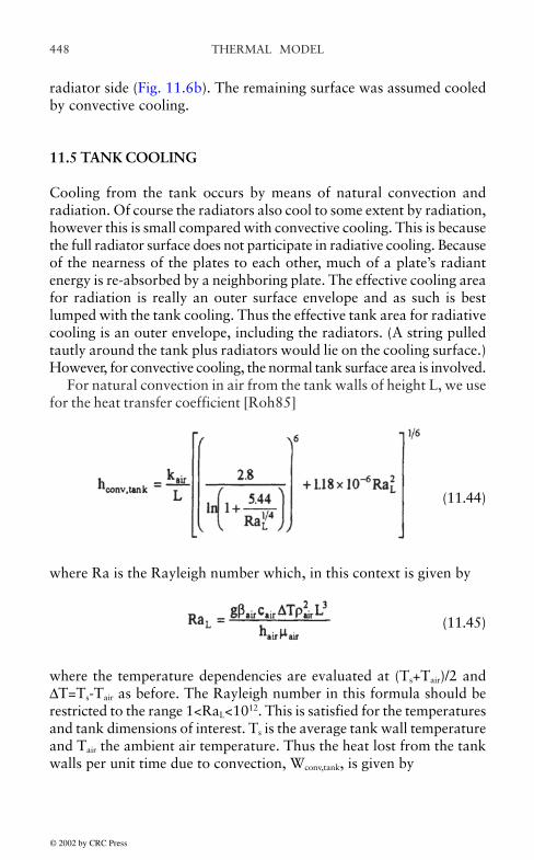
THERMAL MODEL448
radiator side (Fig. 11.6b). The remaining surface was assumed cooledby convective cooling.
11.5 TANK COOLING
Cooling from the tank occurs by means of natural convection andradiation. Of course the radiators also cool to some extent by radiation,however this is small compared with convective cooling. This is becausethe full radiator surface does not participate in radiative cooling. Becauseof the nearness of the plates to each other, much of a plate’s radiantenergy is re-absorbed by a neighboring plate. The effective cooling areafor radiation is really an outer surface envelope and as such is bestlumped with the tank cooling. Thus the effective tank area for radiativecooling is an outer envelope, including the radiators. (A string pulledtautly around the tank plus radiators would lie on the cooling surface.)However, for convective cooling, the normal tank surface area is involved.
For natural convection in air from the tank walls of height L, we usefor the heat transfer coefficient [Roh85]
(11.44)
where Ra is the Rayleigh number which, in this context is given by
(11.45)
where the temperature dependencies are evaluated at (Ts+Tair)/2 and∆T=Ts-Tair as before. The Rayleigh number in this formula should berestricted to the range 1<RaL<1012. This is satisfied for the temperaturesand tank dimensions of interest. Ts is the average tank wall temperatureand Tair the ambient air temperature. Thus the heat lost from the tankwalls per unit time due to convection, Wconv,tank, is given by
© 2002 by CRC Press
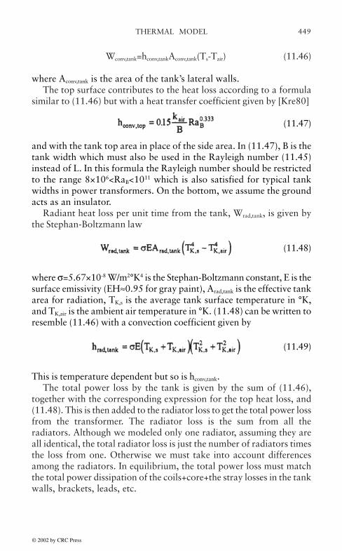
449THERMAL MODEL
Wconv,tank=hconv,tankAconv,tank(Ts-Tair) (11.46)
where Aconv,tank is the area of the tank’s lateral walls.The top surface contributes to the heat loss according to a formula
similar to (11.46) but with a heat transfer coefficient given by [Kre80]
(11.47)
and with the tank top area in place of the side area. In (11.47), B is thetank width which must also be used in the Rayleigh number (11.45)instead of L. In this formula the Rayleigh number should be restrictedto the range 8×10⁶<RaB<1011 which is also satisfied for typical tankwidths in power transformers. On the bottom, we assume the groundacts as an insulator.
Radiant heat loss per unit time from the tank, Wrad,tank, is given bythe Stephan-Boltzmann law
(11.48)
where σ=5.67×10⁻⁸ W/m2°K4 is the Stephan-Boltzmann constant, E is thesurface emissivity (EH≈0.95 for gray paint), Arad,tank is the effective tankarea for radiation, TK,s is the average tank surface temperature in °K,and TK,air is the ambient air temperature in °K. (11.48) can be written toresemble (11.46) with a convection coefficient given by
(11.49)
This is temperature dependent but so is hconv,tank.The total power loss by the tank is given by the sum of (11.46),
together with the corresponding expression for the top heat loss, and(11.48). This is then added to the radiator loss to get the total power lossfrom the transformer. The radiator loss is the sum from all theradiators. Although we modeled only one radiator, assuming they areall identical, the total radiator loss is just the number of radiators timesthe loss from one. Otherwise we must take into account differencesamong the radiators. In equilibrium, the total power loss must matchthe total power dissipation of the coils+core+the stray losses in the tankwalls, brackets, leads, etc.
© 2002 by CRC Press

THERMAL MODEL450
11.6 OIL MIXING IN THE TANK
Perhaps the most complex part of the oil flow in transformers occurs inthe tank. The lack of constraining channels or baffles means that the oilis free to take irregular paths such as along localized circulations oreddies. Nevertheless, there is undoubtedly some overall order in thetemperature distribution and flow pattern. As with any attempt to modela complicated system, we make some idealized assumptions here in aneffort to describe the average behavior of the tank oil.
As shown in Fig. 11.7, we assume that the cold oil at the bottom ofthe tank has a uniform temperature, Tbot, between the bottom radiatordischarge pipe to the tank bottom and that the top oil is at a uniformtemperature, Ttop, from the top of the coils to the top oil level. Wefurther assume that the temperature variation between Tbot and Ttop islinear. This allows us to calculate the average oil temperature along acolumn of oil adjacent to and of equal height as the coils and likewisefor the radiators, determining Tave,out,coils and Tave,out,rads. These twotemperatures will differ because the average radiator vertical positionis above that of the coils. These average temperatures are used indetermining the thermal pressure drop across the coils and radiators asdiscussed previously.
Figure 11.7 Assumed oil temperature distribution inside tank. The oil flows, Q, aswell as the flow weighted temperatures are also indicated.
© 2002 by CRC Press

451THERMAL MODEL
In Fig. 11.7, we have labeled the volumetric oil flows Q withsubscripts c for coils, r for radiators, s for stray loss oil flows, and n fornet. Thus
Qn=Qr-Qc-Qs (11.50)
Qs accounts for the oil flow necessary to cool the core, brackets, tankwalls, etc. Since there is no constraint, mechanical or otherwise, toforce the radiator and coil+stray loss flows to be identical, Qn can differfrom zero. The flow Qc refers to the sum of the flows from all the coilsand Qr the sum from all the radiators.
We have also indicated temperatures associated with some of theflows. The oil flowing into the bottom of the coils is at temperature Tbot
and the oil flowing into the top of the radiators is at temperature Ttop.The temperature of the oil flowing out of the top of the coils, Tc,top, is aflow weighted temperature of the oil from all of the coils. Thus
(11.51)
where i labels the individual coil flows and top temperatures of the oilemerging from the coils. Since we are assuming that all radiators areidentical, Tr,bot is the bottom temperature of the oil exiting a radiator. Ifthe radiators were not all alike, we would use a flow weighted averagefor this temperature also,
We assume, for simplicity, that the volumetric flow Qs, associatedwith the stray power loss Ws, results in a temperature change of ∆T=Ttop-Tbot for the oil participating in this flow. Thus Qs is given by
(11.52)
This is inherently an upward flow and, like the coil flow, is fed by theradiators. We do not attribute any downward oil flow to the tank cooling,but assume that this merely affects the average oil temperature in thetank.
We assume that any net flow, Qn, if positive, results in the transportof cold radiator oil at temperature Tr,bot to the top of the tank and,if negative, results in the transport of hot coil oil at temperature
© 2002 by CRC Press
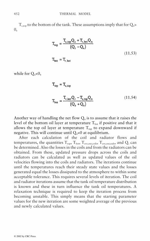
THERMAL MODEL452
Tc,top to the bottom of the tank. These assumptions imply that for Qn>0,
(11.53)
while for Qn<0,
(11.54)
Another way of handling the net flow Qn is to assume that it raises thelevel of the bottom oil layer at temperature Tbot if positive and that itallows the top oil layer at temperature Ttop to expand downward ifnegative. This will continue until Qn=0 at equilibrium.
After each calculation of the coil and radiator flows andtemperatures, the quantities Ttop, Tbot, Tave,out,coils, Tave,out,rads, and Qs canbe determined. Also the losses in the coils and from the radiators can beobtained. From these, updated pressure drops across the coils andradiators can be calculated as well as updated values of the oilvelocities flowing into the coils and radiators. The iterations continueuntil the temperatures reach their steady state values and the lossesgenerated equal the losses dissipated to the atmosphere to within someacceptable tolerance. This requires several levels of iteration. The coiland radiator iterations assume that the tank oil temperature distributionis known and these in turn influence the tank oil temperatures. Arelaxation technique is required to keep the iteration process frombecoming unstable. This simply means that the starting parametervalues for the new iteration are some weighted average of the previousand newly calculated values.
© 2002 by CRC Press

453THERMAL MODEL
11.7 TIME DEPENDENCE
The basic assumption we make in dealing with time dependent conditionsis that at each instant of time the oil flow is in equilibrium with the heat(power) transferred by the conductors to the oil and with the power lossfrom the radiators at that instant. The velocities and oil temperatureswill change with time but in such a way that equilibrium is maintainedat each time step. This is referred to as a quasi-static approximation.The conductor heating, or cooling, on the other hand, is transient. Weassume, however, that the temperature of a disk, which is part of adirected oil flow coil, is uniform throughout the disk so that only thetime dependence of the average disk temperature is treated. A similarassumption is made for non-directed oil flow coils.
The heat generated in a conductor per unit time is I2R, where R is itsresistance (including eddy current effects) at the instantaneoustemperature Tc and I its current. Here conductor refers to a single diskfor a directed oil flow coil and to the entire coil for a non-directed oilflow coil. The transient thermal equation for this conductor is
(11.55)
The left hand side is the heat stored in the conductor of volume V perunit time. This equals the heat generated inside the conductor per unittime minus the heat lost through its surface per unit time. The sum isover all surfaces of the conductor. The other symbols have their usualmeaning with the subscript cond indicating that they refer to theconductor properties. The usual temperature and velocity dependenciesoccur in some of the parameters in (11.55). We solve these equations bya Runge-Kutta technique. These equations replace the steady state diskcoil equations for the Tc (11.31) and, in slightly modified form, one ofthe non-directed oil flow coil equations.
The previous equation accounts for heat (energy) storage in thecurrent carrying conductors as time progresses. Thermal energy is alsostored in the rest of the transformer. We assume, for simplicity, that theremainder of the transformer is at a temperature given by the averageoil temperature. This includes the core, the tank, the radiators, thebrackets or braces, coils not earning current, the insulation, the maintank oil, etc. Thus, the conservation of energy (power) requires that
© 2002 by CRC Press
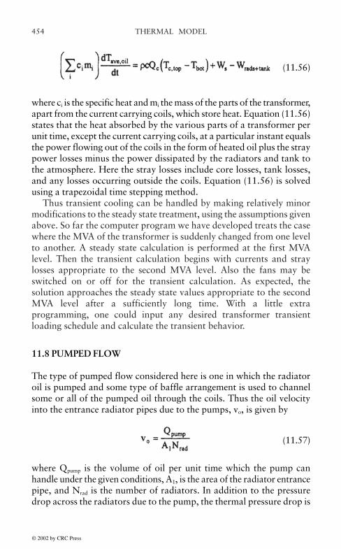
THERMAL MODEL454
(11.56)
where ci is the specific heat and mi the mass of the parts of the transformer,apart from the current carrying coils, which store heat. Equation (11.56)states that the heat absorbed by the various parts of a transformer perunit time, except the current carrying coils, at a particular instant equalsthe power flowing out of the coils in the form of heated oil plus the straypower losses minus the power dissipated by the radiators and tank tothe atmosphere. Here the stray losses include core losses, tank losses,and any losses occurring outside the coils. Equation (11.56) is solvedusing a trapezoidal time stepping method.
Thus transient cooling can be handled by making relatively minormodifications to the steady state treatment, using the assumptions givenabove. So far the computer program we have developed treats the casewhere the MVA of the transformer is suddenly changed from one levelto another. A steady state calculation is performed at the first MVAlevel. Then the transient calculation begins with currents and straylosses appropriate to the second MVA level. Also the fans may beswitched on or off for the transient calculation. As expected, thesolution approaches the steady state values appropriate to the secondMVA level after a sufficiently long time. With a little extraprogramming, one could input any desired transformer transientloading schedule and calculate the transient behavior.
11.8 PUMPED FLOW
The type of pumped flow considered here is one in which the radiatoroil is pumped and some type of baffle arrangement is used to channelsome or all of the pumped oil through the coils. Thus the oil velocityinto the entrance radiator pipes due to the pumps, vo, is given by
(11.57)
where Qpump is the volume of oil per unit time which the pump canhandle under the given conditions, A1, is the area of the radiator entrancepipe, and Nrad is the number of radiators. In addition to the pressuredrop across the radiators due to the pump, the thermal pressure drop is
© 2002 by CRC Press

455THERMAL MODEL
also present and this adds a contribution, although small, to the velocityin (11.57).
We assume that a fraction f of the pumped oil through the radiatorsbypasses the coils. This could be due to inefficient baffling or it could beby design. We also assume that part of the oil flow from the radiators isused to cool the stray losses. This flow, Qs, is given by
(11.58)
where Ws is the stray power loss, Wt, the total loss, and f the fraction ofthe flow bypassing the coils. In addition to the thermal pressure dropacross the coils, a pressure drop due to the pump is present. Atequilibrium, this is determined by the requirement that
Qc=(1-f)Qpump-Qs (11.59)
Thus after each iteration, the flow from all the coils is determined andthe pressure drop across the coils is adjusted until (11.59) is satisfied atsteady-state.
For pumped flow, it is necessary to check for non-laminar flowconditions and to adjust the heat transfer and friction coefficientsaccordingly.
11.9 COMPARISON WITH TEST RESULTS
Computer codes, based on the analysis given in this report, were writtento perform steady state, transient, and pumped oil flow calculations.Although we did not measure detailed temperature profiles along a coil,the codes calculate temperatures of the all the coil disks and of the oil inall the ducts as well as duct oil velocities. Figures 11.8, 11.9, 11.10show these profiles for one such coil having directed oil flow washers.The oil ducts referred to in the figures are the horizontal ducts and theconductor temperature is the average disk temperature. There is thinningin this coil, i.e, increased duct size at two locations, near disk numbers35 and 105, and this can be seen in the profiles. The kinks in the profilesare an indication of the location of the oil flow washers.
© 2002 by CRC Press

THERMAL MODEL456
Figure 11.8 Calculated temperatures of the disks along a disk coil with directed oilflow washers.
Figure 11.9 Calculated average oil temperatures in the horizontal ducts along a diskcoil with directed oil flow washers. The temperature is assumed to vary linearly inthe ducts.
© 2002 by CRC Press

457THERMAL MODEL
As mentioned previously, some leeway was allowed for in thefriction factors for the coils and radiators by including an overallmultiplying factor. This accounts, in an average way, for non idealconditions in real devices and must be determined experimentally. Bycomparing test data with calculations, we determined that the bestagreement is achieved with a multiplying factor of 1.0 for the coils and2.0 for the radiators. Thus the coil friction is close to the theoreticalvalue whereas that for the radiators is twice as high.
Temperature data normally recorded in our standard heat runs are:(1) mean oil temperature rise, (2) top oil temperature rise, (3)temperature drop across the radiators, and (4) average temperature riseof the windings. These are usually measured under both OA and FAconditions. The rises are with respect to the ambient air temperature. Astatistical analysis of such data, taken on a number of transformers withMVAs ranging from 12 to 320, was performed to determine how wellthe calculations and test results agreed. This is shown in Table 11.1where the mean and standard deviations refer to the differences betweenthe calculated and measured quantity. Thus a mean of 0 and a standarddeviation of 0 would indicate a perfect fit. Non zero results for thesestatistical measures reflect both the limitations of the model and someuncertainty in the measured quantities. Table 11.1 shows generallygood agreement between the calculated and measured results. Essentiallyonly one parameter was adjusted in order to improve the agreement,namely the overall friction factor multiplier for the radiators.
Figure 11.10 Calculated velocities of the oil in the horizontal ducts along a disk coilwith directed oil flow washers.
© 2002 by CRC Press

THERMAL MODEL458
Figures 11.11 and 11.12 show representative output from thetransient program in graphical form. In this example, the transformer isoperating at steady state at time 0 at the first MVA value (93 MVA) andsuddenly the loading corresponding to the second MVA (117 MVA) isapplied. The time evolution of the oil temperature is shown in Fig.11.11 while that of one of the coils is shown in Fig. 11.12. The programcalculates time constants and m and n values from this information.Fig. 11.13 shows a direct comparison of the calculated and measuredhot spot temperature of a coil in which a fiber optics temperature probewas imbedded. Although absolute temperatures are off by a fewdegrees, the shapes of the curves are very similar, indicating that thetime constants are nearly the same.
Table 11.1 Comparison of Calculated and Measured Quantities
Figure 11.11 Time evolution of the bottom, average, and top tank oil temperaturesstarting from a steady state loading of 93 MVA at time 0, when a sudden applicationof a 117 MVA loading is applied.
© 2002 by CRC Press

459THERMAL MODEL
Figure 11.12 Time evolution of the average and maximum coil temperature startingfrom a steady state loading of 93 MVA at time 0, when a sudden application of a117 MVA loading is applied.
Figure 11.13 Comparison of calculated and measured temperature versus time of thecoil’s hot spot. The coil is operating at steady state at time 0, when a suddenadditional loading is applied. The hot spot is measured by means of a fiber opticsprobe.
© 2002 by CRC Press

THERMAL MODEL460
11.10 DETERMINING M AND N EXPONENTS
In order to extimate the temperature rises which occur under overloadconditions, approximate empirical methods have been developed whichmake use of the m and n exponents. Although a detailed thermal modelsuch as the one presented above should make these approximationsunnecessary, these exponents are widely used to obtain quick estimatesof the overload temperatures for transformers in service. Although theyare frequently measured in heat run tests, they can also be obtainedfrom either the steady-state or transient calculations of the type presentedabove.
The n exponent is used to estimate the top oil temperature rise abovethe ambient air temperature, ∆Tto, under overload conditions from aknowledge of this quantity under rated conditions. For this estimation,the rated transformer total losses must be known as well as the losses atthe overload condition. The latter losses can be estimated from aknowledge of how the losses change with increased loading and will bediscussed below. The formula used to obtain the overload temperaturerise above ambient is
(11.60)
Thus if 2 refers to the overload condition and 1 to the rated condition,we assume that the 1 subscripted quantities are known either bymeasurement or calculation.
In order to estimate the losses under overload conditions, we mustseparate the losses into I2R resistive losses in the coils and stray losses,which include the core, tank, clamp, and additional eddy current losseswhich occur in the coils due to the stray flux. The I2R loss can becalculated fairly accurately. By subtracting it from the total measuredloss, a good estimate can be obtained for the stray loss. Alternatively,core loss, eddy current loss, tank loss, and clamp loss can be obtainedfrom design formulas. All of these losses depend on on the square of theload current in either winding, (The stray losses depend on the square ofthe stray flux which is proportional to the square of the current,assuming the materials are operating in their linear range.) Since theload current is proportional to the MVA of the unit, these losses areproportional to the MVA squared. The I2R losses are proportional to theresistivity of the winding conductor which is temperature dependent
© 2002 by CRC Press

461THERMAL MODEL
while the stray losses are inversely proportional the the resistivity of thematerial in which they occur. Thus the total loss at the higher loadingcan be obtained from the rated loss by
(11.61)
The resistivity ratios are temperature dependent so that some iterationmay be required with (11.60) to arrive at a self consistent solution. Thestray resistivity ratio is meant to be a weighted average over the materialsinvolved in the stray loss. However since the temperature dependenceof the coil, tank, and clamp materials is nearly the same, this ratio willbe nearly the same as that of the coils.
We should note that the n coefficient is generally measured orcalculated under conditions where the cooling is the same for the ratedand overload conditions. Thus if fans are turned on for the ratedloading, they are also assumed to be on for the overload condition.Similarly if pumps are turned on at the 1 rating, they must also be onfor the 2 rating for the above formulas to work. Although n can bedetermined from measurements or calculations performed at tworatings, it is often desireable to determine it from 3 different loadingsand do a best fit to (11.60) based on these. The 3 ratings generallychosen are usually 70%, 100%, and 125%. The 70%, 100% or 100%,125% combinations are chosen when only 2 ratings are used.Measurements and calculations show that n based on the 70%, 100%combination can be fairly different from n based on the 100%, 125%combination. This suggests that n is not strictly a constant for a giventransformer and it should be determined for loadings in the range whereit is expected to be used. A typical value of n for large powertransformers is 0.9.
The m exponent is defined for each winding and relates the windinggradient to the winding current. The winding gradient at a particularsteady state loading is the temperature difference between the meanwinding temperature and the mean oil temperature in the tank, i.e.
Gradient=Mean winding temperature-Mean Tank oil temperature(11.62)
© 2002 by CRC Press

THERMAL MODEL462
Letting 1 and 2 designate rated and overload conditions, the m coefficientfor a particular winding relates the gradients to the winding currents by
(11.63)
Since the currents are proportional the the MVA’s, the MVA ratio couldbe substituted in the above formula for the current ratio. The m exponentscan be determined from 2 or 3 MVA loadings and, like the n exponent,depend to some extent on the MVA range covered. They also can varyconsiderably for different windings. A typical value for large powertransformers is about 0.8.
The winding gradient is often used to estimate the winding’smaximum temperature. A common procedure is to add some multipleof the gradient to the top oil temperature to arrive at the maximumtemperature for that winding, for example
Max winding temp=Top oil temp+1.1×Winding Gradient (11.64)
The factor of 1.1 can differ among manufacturers or transformer typesand should be determined experimentally. Formulas such as (11.64)become unnecessary when detailed temperature calculations are availableor maximum temperatures are measured directly by fiber optics orpossibly other types of temperature probes, inserted into the winding atits most probable location. Detailed temperature calculations such asdescribed above can provide some guidance as to where these probesshould be inserted.
11.11 LOSS OF LIFE CALCULATION
Although transformers can fail for a number of reasons such as from theapplication of excessive electrical or mechanical stress, even a highlyprotected unit will eventually fail due to aging of its insulation. Whilethe presence of moisture and oxygen affect the rate of insulation aging,these are usually limited to acceptable levels in modern transformers sothat the main factor affecting insulation aging is temperature. Theinsulation’s maximum temperature, called the hot spot temperature, isthus the critical temperature governing aging. This is usually the highestof the maximum temperatures of the different windings, although it
© 2002 by CRC Press

463THERMAL MODEL
could also be located on the leads which connect the windings to thebushings or to each other.
Numerous experimental studies have shown that the rate ofinsulation aging as measured by various parameters such as tensilestrength or degree of polymerization (DP) follows an Arrheniusrelationship,
K=Ae-B/T (11.65)
Here K is a reaction rate constant (fractional change in quantity perunit time), A and B are parameters, and T is the absolute temperature.For standard cellulose pased paper insulation, B=15000°K. This valuefor B is an average from different studies using different properties todetermine aging [McN91]. If X is the property used to measure aging,e.g. tensile strength of DP, then we have
X(t)=X(t=0)e-Kt (11.66)
The time required for the property X to drop to some fraction f of itsinitial value if held at a constant temperature T, tT, is thus determinedby
(11.67)
Taking logarithms, we obtain
(11.68)
where (11.65) has been used.There are several standard or normal insulation lifetimes which
have found some acceptance. For these, the insulation hot spot isassumed to age at a constant temperature of 110°C. The insulation isalso assumed to be well dried and oxygen free. Under these conditions,the time required for the insulation to retain 50% of its initial tensilestrength is 7.42 years (65000 hours), to retain 25% of its initial tensilestrength is 15.41 years (135000 hours), and to retain a DP level of 200is 17.12 years (150000 hours). Any of these criteria could be taken as ameasure of a normal lifetime, depending on the experience or the
© 2002 by CRC Press

THERMAL MODEL464
degree of conservatism of the user However, if the transformer isoperated at a lower temperature continuously, the actual lifetime can beconsiderably longer than this. For example, if the hot spot is kept at95°C continuously, the transformer insulation will take 36.6 years to beleft with 50% of its initial tensile strength. Conversely, if operated athigher temperatures, the actual lifetime will be shortened.
Depending on the loading, the hot spot temperature will vary overthe course of a single day so that this must be taken into account indetermining the lifetime. A revealing way of doing this is to comparethe time required to produce a fractional loss of some material propertysuch as tensile strength at a given temperature with the time required toproduce the same loss of the property at the reference temperature of110 °C. Thus the time required to produce the fractional loss f in thematerial property at temperature T is given by (11.68) and the time toproduce the same fractional loss at the reference temperature,designated To , is given by the same formula with To replacing T. Thislatter time will be designated tTo. Hence we have for the given fractionalloss,
(11.69)
We have defined the aging acceleration factor, AAF , in (11.69), Thusit requires AAF(T) times as much time at the reference temperaturethan at temperature T to produce the same fractional loss of life asdetermined by property X. Since the T’s are in °K, we have
(11.70)
AAF is > or <1 depending on whether T(°C) is > or <110°C. This isplotted in Fig. 11.14.
© 2002 by CRC Press

465THERMAL MODEL
A method of using the daily variations of hot spot temperature tocompute aging is to subdivide the day into (not necessarily equal) timeintervals over which the hot spot temperature is reasonably constant.Let AAFi be the aging acceleration factor for time interval ∆ti measuredin hours. Then for a full day
(11.71)
where N is the total number of time intervals for that day.The actual loss of life will depend on the definition of lifetime. If the
50% retained tensile strength criterion is uned, then in 1 day at 110°Cinsulation hot spot temperature, the transformer loses the fraction 24/65000=3.69×10-4 of its life. The fraction lost with variable hot spottemperature is therefore AAFday ave×3.69×10⁻⁴. For the 25% retainedtensile strength criterion, the loss of life for 1 day is AAFday ave×1.78×10⁻⁴.
A cautionary note must be sounded before too literal a use is made ofthis procedure. Gas bubbles can start to form in the oil next to theinsulation when the insulation temperature reaches about 140°C. These
Figure 11.14 Aging Acceleration Factor (AAF) relative to 110°C vs temperature.
© 2002 by CRC Press

THERMAL MODEL466
bubbles can lead to dielectric breakdown which could end thetransformer’s life, rendering the calculations inapplicable.
There is bound to be some uncertainty involved in determining thehot spot temperature unless fiber optics or other probes are used andproperly positioned. Short of this, it should be estimated as best aspossible, based on top oil temperature, winding gradients, etc. Also awinding temperature indicator, if properly calibrated, can be used.
Since the AAF is independent of the choice made for the normaltransformer lifetime, the fractional loss of life can be easily recalculatedif a different choice of normal lifetime is made based on additionalexperience or knowledge.
11.12 CABLE AND LEAD TEMPERATURE CALCULATION
Although the conductors in the coils are usually cooled sufficiently tomeet the required hot spot limits, it is also necessary to insure that thelead and cable temperatures remain below these limits as well. Eventhough these are generally not in critical regions of electric stress tocause a breakdown if gassing occurs, the gassing itself can trigger alarmswhich could put the transformer out of service. It is thus necessary forthe design engineer to insure that the leads and cables are sized to meetthe temperature requirements.
In general, no more insulation (paper) should be used on the leadsand cables than is necessary for voltage standoff. Given this minimumpaper thickness, the current carrying area of the lead or cable shouldthen be chosen so that the temperature limits are met when rated currentis flowing. A method for calculating the lead or cable temperature riseis given here. It allows for the possibility that the lead is brazed to acable and that some heat conduction can occur to the attached cable,acting as a heat sink. It also considers the case of a lead inside of duct ortube or a lead in the bulk transformer oil.
We treat a cylindrical geometry. In the event the lead is notcylindrical, an effective diameter should be calculated so that it may beapproximated by a cylinder. The cylinder is assumed to be long so thatend effects may be neglected. The geometric parameters are shown inFig. 11.15.
© 2002 by CRC Press

467THERMAL MODEL
The convective heat transfer coefficient of the oil is denoted by h.The thermal conductivities of the conductor and paper are denoted kc
and kp respectively and the power generated per unit volume inside theconductor is denoted by qv. This is given by the Joule loss density, ρ J2,where ρ is the resistivity and J the rms current density. In addition, toaccount for extra losses due to stray flux, we should multiply this by(1+f) where f is the stray flux loss contribution expressed as a fraction ofthe Joule losses.
There are two cases to consider for the convective heat transfercoefficient of the oil. They are the case of a horizontal cylinder in freetank oil and the case of a horizontal cylinder inside of a channel. (Theheat transfer coefficient for a vertical cylinder is higher so the resultingtemperature rises will be lower than for a horizontal cylinder.) Theseare given by [Kre80]:
Natural convection from a horizontal cylinder of diameter D in bulkfluid:
(11.72)
Figure 11.15 Cylindrical geometry of a paper wrapped conductor surrounded by oil
© 2002 by CRC Press

THERMAL MODEL468
Mixed natural convection and laminar flow in horizontal ducts:
(11.73)
where the symbols have the following meaning:
Nusselt number
Reynold’s number
Prandtl number
Grashof number
Graetz number
v=fluid velocityD=hydraulic diameter for flow inside ducts=4×flow area/wettedperimeter=outer cylinder diameter for external flowL=duct or cylinder lengthg=acceleration of gravity=9.8 m/sec2
h=convective heat transfer coefficientk=thermal conductivity of transformer oil=0.11 W/m°Cc=specific heat of transformer oil=1880 J/kg°Cµ=oil viscosity=6900.0/(T+50)3 Ns/m2, T=temp in °Cρm=oil mass density=867 exp(-0.00068 (T-40)) kg/m3, T= temp in °Cβ=volume expansion coefficient of oil=0.00068/°CSubscripts s and b label the oil at the outside surface of the paper andthe bulk oil
© 2002 by CRC Press

469THERMAL MODEL
In steady state, the thermal equations governing this situation are
Inside conductor,
(11.74)
Inside paper,
(11.75)
The boundary conditions are:
At r=0,
At r=r1, Tc=Tp and
At r=r2,
where c labels the temperature inside the conductor and p inside thepaper. The solution is given by
(11.76)
(11.77)
The highest temperature occurs at r=r1 and is given, in terms oftemperature rise above the bulk oil, by
(11.78)
The quantity qv r1/2 is a surface heat flux, qs, since
© 2002 by CRC Press

THERMAL MODEL470
(11.79)
where L is the cylinder length which cancels. Thus (11.78) has the form
qs=heff (Tc(r1)-Tb) (11.80)
where
(11.81)
is an effective heat transfer coefficient which takes into accountconduction through the paper. In the case of a thin paper layer of thicknessτ where and r2=r1+τ, (11.81) reduces to
(11.82)
This last expression also applies to a planar geometry. Note that thesurface heat flux in (11.81) is based on the surface area of a cylinder ofradius r1, i.e. that of the metallic part of the cable. We also need thetemperature rise of the surface oil in order to compute the Grashof number.This is given by
(11.83)
so that, comparing (11.78) and (11.83), we can write
(11.84)
so that the temperature rise of the surface paper can be found once themaximum conductor temperature rise is calculated.
© 2002 by CRC Press

471THERMAL MODEL
where
Tc=conductor surface temperatureTb=bulk fluid temperatureTcable=brazed on cable temperaturep=perimeter of the conductor’s cooling surfaceAside=pL=conductor’s side area through which heat flows to the coolingfluidAcond=conductor’s current carrying areahcond=kcu/L=heat transfer coefficient for heat to flow from the conductorto the brazed on cable. For copper kcu=400 W/m°C.
In order to use the above expression to obtain the lead temperature rise,the temperature rise of the cable must be calculated first. Since the cableis normally very long, its temperature rise can be obtained by neglectingits brazed connection.
In case another cable is brazed to the conductor which may act as aheat sink, we must consider heat conduction along the conductor to theother cable. The situation is depicted in Fig. 11.16.
Figure 11.16 Geometry and thermal parameters for a cable or lead with anotherbrazed to it
Letting W=the total power dissipated inside the conductor of length L,we have
(11.85)
© 2002 by CRC Press

THERMAL MODEL472
Although we have indicated the numerical value of most of thematerial parameters in the preceding section, the missing ones will begiven here. They are:
Thermal conductivity of paper kp=0.16 W/m°CResistivity of copper ρ=1.72×10⁻⁸(1+0.004 (T-20)), T in °C v=oil velocityin duct=0.1 in/sec=0.00254 m/sec (This is a conservative value. If abetter value can by obtained, e.g. from an oil flow calculated in thecooling program, then it should be used.)
In addition, it should be noted that many of these material parametersare temperature dependent so that it is necessary specify a bulk oiltemperature and to iterate the calculations. The appropriate temperatureto use for evaluating the oil parameters is (Ts+Tb)/2, i.e. the average ofthe surface and bulk oil temperatures. For the conductor, its temperatureis nearly uniform so its maximum temperature can be used. The Grashofnumber depends on the temperature difference Ts-Tb so it must berecalculated during the iteration process along with the other materialparameters.
These formulas have been applied to some standard cable sizes toobtain the maximum continuous currents permissible for a hot spottemperature rise of about 25°C. We assumed an oil temperature rise of55°C above an ambient air temperature of 30°C resulting in a bulk oiltemperature of 85°C. Thus a rise of 25°C would result in a hot spottemperature of 110°C. The results are shown in Table 11.2. Note thatthe conductor area does not fill 100% of the geometrical area of thecable since the conductor is stranded.
© 2002 by CRC Press

473THERMAL MODEL
11.13 TANK WALL TEMPERATURE CALCULATION
Heating in the tank wall above the adjacent oil temperature is due toeddy currents induced by the stray leakage flux from the main coils andflux from any nearby leads or busses. Generally a chief cause for concernis the presence of high current carrying leads near the tank wall. Wehave indicated how these may be calculated in Chapter 10. Here we aregoing to assume that these losses are known and that they are uniformlydistributed throughout the tank wall. We will also assume that the tankwall surface dimensions involved are large compared with the tankwall thickness so that only 1 spatial dimension through the wall thicknessis important. Fig. 11.17 shows the geometric and other releventparameters.
Table 11.2 Maximum Continuous rms Currents for Standard Cable Sizes producinga Temperature Rise Above the Surrounding Oil of 25°C
© 2002 by CRC Press

THERMAL MODEL474
Here L is the wall thickness, qv the losses generated in the tank wall perunit volume, k the thermal conductivity of the tank wall material, h1 theheat transfer coefficient from the tank wall to the oil, h2 the heat transfercoefficient from the tank to the air, and T(x) the temperature distributionin the tank wall.
The steady state thermal equation for this situation is given by
(11.86)
with the boundary conditions
(11.87)
The different signs in the two boundary conditions are necessary toproperly account for the direction of heat flow. The solution can beexpressed as
Figure 11.17 Tank wall geometry and thermal parameters
(11.88)
© 2002 by CRC Press

475THERMAL MODEL
This expression can be simplified by noticing that thermal transfer withinthe tank wall is much larger that that at the surface. This means that kis much larger than h1L or h2L so that, ignoring terms ≤1 relative to k/h1L or k/h2L, (11.88) becomes
(11.89)
This is independent of x so that the tank wall temperature is essentiallyuniform throughout and we have written Ttank for it. The last term onthe right is the weighted average of the oil and air temperatures, weightedby their respective heat transfer coefficients. The first term on the rightaccounts for the heat generated in the tank wall. We can use the heattransfer coefficients given in Section 11.5 on Tank Cooling. Anotherexpression which could be used for heat transfer due to natural convectionfrom one side of a vertical plate of height H immersed in a fluid (air oroil) is given by [Kre80]
(11.90)
where the Grashof and Prandtl numbers have been defined in Section11.12. This expression holds for 109<GrHPr<1013. To this, one wouldhave to add the radiation term to the air heat transfer coefficient.
As a numeric example, let h1=hoil=70 W/m2°C, h2=hair+hrad= 13 W/m2°C, k=ksteel=40 W/m°C, L=9.525×10⁻³ m (0.375 in). From these weobtain k/h1L=60 and k/h2L=323. Both of these are much larger than 1 sothat the approximate formula (11.89) may be used. Letting qv=2×10⁵ W/m3, Toil=85°C, Tair=30°C, we obtain Ttank= 99.3°C.
11.14 TIEPLATE TEMPERATURE CALCULATION
Tieplate losses were calculated in Chapter 10. These losses must beobtained by some method, such as that described there, in order tocalculate the tieplate’s surface temperature. In order to make thistemperature calculation tractable analytically, we make some idealizedassumptions which appear to be reasonable. We assume the plate isinfinite in two dimensions and that the losses fall off exponentially fromthe surface facing the coils in the other dimension. The exponential
© 2002 by CRC Press

THERMAL MODEL476
drop-off is determined by the skin depth and has the form e-x/τ where x isthe distance from the free surface and is the skin depth. The surfacefacing the coils is assumed to be cooled convectively by the oil with aheat transfer coefficient h. The boundary condition on the other surfacefacing the core will depend on the construction details which may differamong manufacturers. We will assume that there is a cooling gap herebut that the heat transfer coefficient may be different from that at theother surface. To allow for an insulated core facing surface, this heattransfer coefficient may simply be set to zero. This geometry and thecooling assumptions are identical to that assumed for the tank walltemperature calculation. However here we are allowing for anexponential drop off of the loss density which is more realistic in thecase of soft steel tieplates. Thus we are using the geometric and thermalparameters of Fig. 11.17 except that air now refers to oil cooling on thesurface at a distance x=L, where L is the tieplate thickness. Tieplateshave a finite width and we are ignoring the enhanced loss density at thecorners which is evident in the finite element study for soft steel ofChapter 10. However there is also extra cooling at the corner from theside surface which could mitigate the effect of this extra loss density.One could address this problem by means of a thermal finite elementprogram. However, the analytic solution presented below should applyto temperatures away from the corner and these may possibly be higheror comparable to the corner temperature.
This is a 1-dimensional steady-state heat transfer problem. Thedifferential equation to solve is the same as (11.86) in the previoussection. However, here we have , where qvo is the lossdensity at the surface at x=0 and τ is the skin depth, rather than theconstant assumption for qv used for tank cooling. Thus the side facingthe coils is at x=0. The boundary conditions are the same as (11.87)with the air subscript replaced by oil. The solution is
We have expressed the solution is this form so that the case of an insulatedback side (h2=0) could be easily obtained. From (11.91) we can obtainthe surface temperature rise at the x=0 surface,
(11.91)
© 2002 by CRC Press
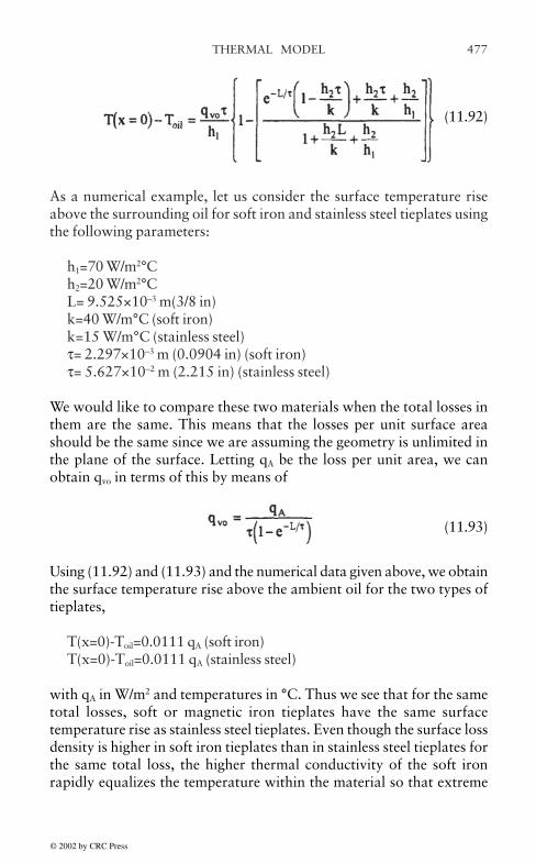
477THERMAL MODEL
As a numerical example, let us consider the surface temperature riseabove the surrounding oil for soft iron and stainless steel tieplates usingthe following parameters:
h1=70 W/m2°Ch2=20 W/m2°CL= 9.525×10⁻³ m(3/8 in)k=40 W/m°C (soft iron)k=15 W/m°C (stainless steel)τ= 2.297×10⁻³ m (0.0904 in) (soft iron)τ= 5.627×10⁻² m (2.215 in) (stainless steel)
We would like to compare these two materials when the total losses inthem are the same. This means that the losses per unit surface areashould be the same since we are assuming the geometry is unlimited inthe plane of the surface. Letting qA be the loss per unit area, we canobtain qvo in terms of this by means of
(11.93)
Using (11.92) and (11.93) and the numerical data given above, we obtainthe surface temperature rise above the ambient oil for the two types oftieplates,
T(x=0)-Toil=0.0111 qA (soft iron)T(x=0)-Toil=0.0111 qA (stainless steel)
with qA in W/m2 and temperatures in °C. Thus we see that for the sametotal losses, soft or magnetic iron tieplates have the same surfacetemperature rise as stainless steel tieplates. Even though the surface lossdensity is higher in soft iron tieplates than in stainless steel tieplates forthe same total loss, the higher thermal conductivity of the soft ironrapidly equalizes the temperature within the material so that extreme
(11.92)
© 2002 by CRC Press

THERMAL MODEL478
temperature differences cannot develop. If the back surface were insulated(h2=0), all the losses would have to leave the front surface in the steadystate. In this case also the surface temperatures of the soft iron andstainless steel tieplates would be identical for the same total loss. As h2
increases up to h1, the front surface temperatures gradually differ for thetwo cases but not significantly.
11.15 CORE STEEL TEMPERATURE CALCULATION
Because core steel is made up of thin stacked insulated laminations, ithas an anisotropic thermal conductivity. The thermal conductivity inthe plane of the laminations is much higher than the thermal conductivityperpendicular to this plane or in the stacking direction. The steadystate heat conduction equation for this situation is, in rectangularcoordinates,
(11.94)
where the thermal conductivities k can differ in the x and y directionsare are labelled accordingly. The loss per unit volume, qv, is assumed tobe a constant here. Again there are finite element programs which cansolve this equation for complex geometries such as a stepped core. Wewill derive a simple but approximate analytical solution here for arectangular geometry as shown in Fig. 11.18.
Figure 11.18 Rectangular geometry for anisotropic thermal calculation
© 2002 by CRC Press

479THERMAL MODEL
This could apply to one step of a core, say the central step, withcooling ducts on the long sides or to all or part of a core between twocooling ducts by suitably calculating effective dimensions for anapproximating rectangle from the steps involved.
We look for a solution of (11.94) of the form
T=A+Bx+Cx2+Dy+Ey2 (11.95)
satisfying the boundary conditions at the center
(11.96)
This is required by symmetry. At the outer surfaces, we onlyapproximately satisfy the boundary conditions for convective cooling
(11.97)
This means that we are satisfying the convective boundary conditionexactly only at the surface points on the two axes. However, this iswhere we will evaluate the surface temperature. The solution is
(11.98)
Note that a and b are 1/2 the rectangle dimensions. We can estimate thethermal conductivity in the direction perpendicular to the laminationplane (the y-direction here) from a knowledge of the coating thicknessor stacking factor and the thermal properties of the coating. For stacked
© 2002 by CRC Press

THERMAL MODEL480
silicon steel we use kx=30 W/m°C and ky=4 W/m°C. Letting h=70 W/m2°C for convective oil cooling and assuming an effective stack orrectangle size of 0.762 m (30 in)×0.254 m (10 in) and using qv=104 W/m3 (1.3 W/kg, 0.6 W/1b), we find for the maximum internal temperaturerise above the surrounding oil T(0.0)-Toil=25.8°C. The surface temperaturerise in the x or long dimension is T(a,0)-Toil= 17.8°C and the surfacetemperature rise at the surface at y=b in the short direction perperdicularto the stack is T(0,b)-Toil=12.2°C. Note that the surface in the directionof lower thermal conductivity is actually cooler than the surface towardswhich heat is more easily conducted. This is because, the centraltemperature being the same, there is a smaller thermal gradient in thehigh conductivity direction relative to the lower one.
© 2002 by CRC Press

481
12. LOAD TAP CHANGERS
Summary Load tap changers are a major component of manytransformers. They are used to change the voltage of the primary orsecondary side of a transformer to compensate for voltage variations inthe power system mainly caused by variable loading. We discussgenetically the various types of load tap changers and some of theimportant ways they are connected to the primary or secondary windingsas well as the advantages and disadvantages of these connection schemes.We also address some of the maintanence issues which are of interest tothe user.
12.1 INTRODUCTION
The flicker of the house lights while having dinner is a sign of a load tapchanger (LTC) tap change. When most people get home from work,they start using electricity for cooking and lighting. This increases theelectrical load on the distribution network, which causes the voltage tosag below its nominal value. The latter signals the LTC to change tapsto adjust the voltage back to its nominal value with some tolerance.
There are many applications of transformers in modern electricpower systems: from generator step-up to system interconnection todistribution to arc-furnace to HVDC converters to mention just a few.The role of a transformer is to convert the electrical energy from onevoltage level to another. As power systems become larger and morecomplex, power transformers play a major role in how efficient andstable the system is. For each transformer installed in a network, thereis an ideal (optimal) voltage ratio for an optimal operation of thesystem. Unfortunately, this optimal voltage ratio varies depending onthe operating conditions of the total network. Early in the history ofelectric power systems, it became evident that for power systems tooperate satisfactorily, transformer voltage ratios needed to beadjustable without interrupting the flow of energy. This is the role of aload tap changer.
© 2002 by CRC Press

LOAD TAP CHANGERS482
12.2 GENERAL DESCRIPTION OF LTC
A load tap changer is a device that connects different taps of tappedwindings of transformers without interrupting the load. It must be capableof switching from one tap position to another without at any timeinterrupting the flow of the current to the load and without at any timecreating a short-circuit between any two taps of the transformer winding.Tap changing transformers are used to control the voltage or the phaseangle or both in a regulated circuit.
A LTC is made of 4 elements:
1) A selector switch which allows the selection of the active tap2) A change-over switch, referred as a reversing switch when it reverses
the polarity of the tapped winding, used to double the number ofpositions available
3) A transition mechanism, including an arcing or diverter switch,which effects the transition from one tap to the other
4) A driving mechanism which includes a motor and gear box andcontrols to drive the system
There are 2 generic types of tap changers:
In-tank
The cover mounted, in-tank tap changer, known as the Jansen type, sitsin the main transformer oil together with the core-and-coil assembly. Itsselector and change-over switches are at the bottom of the tap changerin the main oil. The arcing (diverter) switch is located in a separatecompartment at the top, usually within a sealed cylinder made offiberglass or other similar material. All arcing is confined to thiscompartment. They exist in single phase or three phase neutral end Wye(Y) connected versions. For three phase folly insulated applications,three single phase tap changers must be used. This type of tap changeris used for higher voltages or current levels.
Separate compartment
The side mounted, separate compartment types have their own box andare assembled separately from the transformer. They are bolted to theside of the tank and connected to the transformer tapped windings througha connecting board. Their selector, change-over, and arcing switchesare located in an oil compartment completely isolated from the main
© 2002 by CRC Press
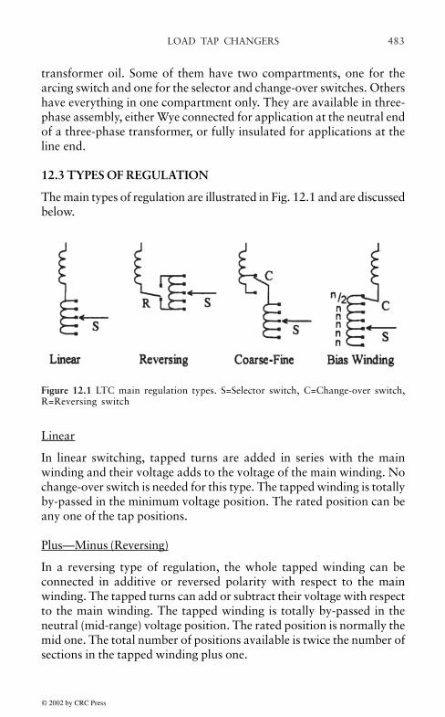
483LOAD TAP CHANGERS
transformer oil. Some of them have two compartments, one for thearcing switch and one for the selector and change-over switches. Othershave everything in one compartment only. They are available in three-phase assembly, either Wye connected for application at the neutral endof a three-phase transformer, or fully insulated for applications at theline end.
12.3 TYPES OF REGULATION
The main types of regulation are illustrated in Fig. 12.1 and are discussedbelow.
Linear
In linear switching, tapped turns are added in series with the mainwinding and their voltage adds to the voltage of the main winding. Nochange-over switch is needed for this type. The tapped winding is totallyby-passed in the minimum voltage position. The rated position can beany one of the tap positions.
Plus—Minus (Reversing)
In a reversing type of regulation, the whole tapped winding can beconnected in additive or reversed polarity with respect to the mainwinding. The tapped turns can add or subtract their voltage with respectto the main winding. The tapped winding is totally by-passed in theneutral (mid-range) voltage position. The rated position is normally themid one. The total number of positions available is twice the number ofsections in the tapped winding plus one.
Figure 12.1 LTC main regulation types. S=Selector switch, C=Change-over switch,R=Reversing switch
© 2002 by CRC Press

LOAD TAP CHANGERS484
Coarse—Fine
The coarse-fine regulation can be defined as a two-stage linear regulationwhere the first or coarse stage contains a large number of turns whichcan be totally by-passed by the change-over selector. These turns areshown as a single loop in the top coil of the figure. Fine regulation isachieved with the selector switch. Normally, the coarse section containsas many turns as the tapped winding plus one section. In that way, thetotal number of positions available is twice the number of sections inthe tapped winding plus one.
Bias winding
The bias winding type of regulation is similar to the coarse-fine exceptthat the number of turns in the bias winding is half the turns of onesection of the tapped winding. It is used to provide half steps betweenthe main tap steps. Thus the total number of positions available is twicethe number of sections in the tapped winding plus one. The bias windingtechnique can be combined with the reversing scheme to provide twicethe number of positions (four times the number of sections in the tappedwinding plus one) at the expense of adding one more switch andincreasing the complexity of the switching and driving mechanism.
Although not indicated in the figure, the tap selector switch is often acircular type of switch to allow a smooth transition between the tapvoltages when the change-over or reversing switch operates.
12.4 PRINCIPLE OF OPERATION
A load tap changer must be capable of switching from one tap positionto another without interrupting the flow of current to the load at anytime. It must therefore follow a “make before break” switching sequence.On the other hand, it cannot at any time create a short-circuit betweenany two taps of the transformer winding. This means that during thismake before break interval, there must be something to prevent theshorting of the turns. Two ways are primarily used to accomplish this.
12.4.1 Resistive Switching
Fig. 12.2 shows an example of a six step switching sequence. Thisparticular type of tap changer has two selector switches and an arcingswitch with four contacts.
© 2002 by CRC Press

485LOAD TAP CHANGERS
1) Step 1 of the figure above shows the steady state of the TC justbefore the switching operation. The load current is flowing throughthe contact #1 and the selector #1. Let us call that position tap #2.
2) At step 2, the non-conducting selector has moved 2 steps down,from position 1 to position 3. The current is still flowing in contact#1 and the selector #1.
3) At step 3, the contact #1 opens and the current flows throughresistor #1 and selector #1.
4) At step 4, the contact #3 closes and the current splits between the2 resistors and the 2 selectors. There is also a circulating current
Figure 12.2 Sequence of operations involved in tap changers using resistive switching.The selector switches are the top most switches. The arcing switches are closed whena diagonal (shorting) line is present and open otherwise.
© 2002 by CRC Press

LOAD TAP CHANGERS486
flowing into the loop limited by the 2 resistors and the reactanceof the loop.
5) At step 5, the contact #2 opens, breaking the current in the resistorand selector #1. It is at that moment that arcing occurs, The arcremains on until the current crosses the zero line. At worst, it canlast one half cycle which, at 60 Hz, is 8 msec. The average arcingtime is around 5 to 6 msec.
6) At step #6, the contact #4 closes and the load current by-passes theresistor #2 and goes directly to the selector #2. The TC has reachedthe steady state for tap position #3.
This type of transition requires that the resistors be capable ofwithstanding the full load current plus the circulating current during thetransition (from step 3 to step 5). In order to reduce the energy absorptionrequirement for the resistors, the time of the complete transition has tobe minimized. These tap changers have normally very fast transitions.
12.4.2 Reactive Switching with Preventative Autotransformer
Another widely used way of handling the transition from one tap toanother is to use reactors instead of resistors. These reactors do not haveto dissipate as much energy as the resistors. They mainly use reactiveenergy, which does not produce any heat. Therefore, they can be designedto withstand the full load plus the circulating current for long periods oftime, even continuously. Two reactors per phase are needed. They arenormally wound on a common gapped core, making them mutuallycoupled. When they are connected in series, they act as an auto-transformer. When they are connected in parallel, they act as a singlereactor. Transformer designers take advantage of this feature. They usethe reactors not only to prevent the load current from being interruptedor to prevent sections of a tapped winding from being shorted, but alsoto act as a transformer and provide intermediate voltage steps in betweentwo consecutive tap sections of the main transformer. The total numberof positions available with this scheme is twice the number of sectionsin the tapped winding plus one. Here is how it works.
The method of operation is diagrammed in Fig. 12.3, The tapchanger has two selectors, two reactors (actually one reactor with 2windings), two by-pass switches (#1 and #2) and an arcing switch (#3).
© 2002 by CRC Press

487LOAD TAP CHANGERS
1) In step 1 of the figure above, the tap-changer is in the steady statemode on tap position #2. The load current flows in the 2 selectors,the 2 reactors and the by-pass switches. Although the arcing switchis closed, no current flows through it.
2) In step 2, the by-pass switch opens. The current flows through theswitch #1, and then splits up between the 2 reactors and the 2selectors.
3) In step 3, the arcing switch opens. All current flows through thereactor 1 and the selector 1. Arcing occurs at that step because thecurrent in the reactor is interrupted.
Figure 12.3 Sequence of operations involved in tap changers using reactive switching
© 2002 by CRC Press

LOAD TAP CHANGERS488
4) In step 4, the right selector moves one step to the right, while itcarries no current.
5) In step 5, the arcing switch closes, causing current to flow again inthe reactor #2 and in selector #2. Note that the two selectors areon different taps. This causes a circulating current to flow into theloop.
6) In step 6, the by-pass switch #2 closes and a steady state conditionis reached, which is in this case tap position #1. Because the 2ends of the reactors are on 2 different taps, they are in seriesbetween the 2 taps. The voltage at their mid point is halfwaybetween the 2 taps. This state is called the “bridging position”,where the reactors bridge between 2 taps.
When combined with a reversing switch, this scheme provides four timesas many voltage positions as tapped sections in the winding plus one.The price to pay is that the reactor has to be designed to withstandcontinuously the full load current plus the circulating current; the tappedwinding has also to withstand the full load plus the circulating current;and the reactor introduces losses and draws more magnetizing currentfrom the source, specially on bridging positions. It might also add audiblenoise to the transformer.
12.5 CONNECTION SCHEMES
12.5.1 Full Transformers
Normally, the primary winding of transformers is fed at a constantvoltage and the role of the tap changer is to add or subtract turns inorder to vary the voltage ratio of the transformer to maintain its outputat a constant voltage despite fluctuations in the load current. In principle,this can be accomplished by changing the number of active turns eitherin the primary or secondary winding. There are subtle differences in thetwo ways of connecting the tap changer which transformer and systemdesigners have to be aware of.
Fixed volts/turn
The most natural way to add a tapped winding to a transformer is toconnect it in series with the regulated side. As shown in Fig. 12.4, theprimary winding of the transformer (H1–H2) is fed at a constant voltageand it has a fixed number of turns. So the volts/turn of the transformer is
© 2002 by CRC Press

489LOAD TAP CHANGERS
constant. The voltage across X1-X2 varies with the number of turns. Ifall the taps have equal number of turns, then the voltage increase isequal for each step. If the X winding is Wye connected, then the tappedwinding and the tap changer can be placed at the low potential neutralend and do not require a high insulation level. The price to pay is thatthe tap changer has to be capable of carrying the current of the X winding.For high current windings, the cost of such a tap changer could becomeprohibitive. Another disadvantage is that low voltage windings oftenhave few turns. The design of the tapped winding might becomeimpractical if not impossible considering that fractional turns cannot beused.
Figure 12.4 Fixed volts/turn tap changing scheme
Variable volts/turn
One way to solve the problem of high current low voltage windings isto put the tapped winding in the high voltage side. The low voltageside can still be regulated in this way. This is particularly applicable ifthe HV is Wye connected since the tap changer could be placed at theneutral end and would not require a high insulation level while notcarrying a high current. This scheme is illustrated in Fig. 12.5
Figure 12.5 Variable volts/turn tap changing scheme
© 2002 by CRC Press
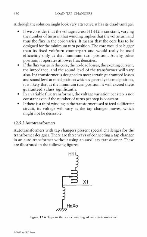
LOAD TAP CHANGERS490
Although the solution might look very attractive, it has its disadvantages:
• If we consider that the voltage across H1-H2 is constant, varyingthe number of turns in that winding implies that the volts/turn andthus the flux in the core varies. It means that the core has to bedesigned for the minimum turn position. The core would be biggerthan its fixed volt/turn counterpart and would really be usedefficiently only at that minimum turn position. At any otherposition, it operates at lower flux densities.
• If the flux varies in the core, the no-load losses, the exciting current,the impedance, and the sound level of the transformer will varyalso. If a transformer is designed to meet certain guaranteed lossesand sound level at rated position which is generally the mid position,it is likely that at the minimum turn position, it will exceed theseguaranteed values significantly.
• In a variable flux transformer, the voltage variation per step is notconstant even if the number of turns per step is constant.
• If there is a third winding in the transformer used to feed a differentcircuit, its voltage will vary as the tap changer moves, whichmight not be desirable.
12.5.2 Autotransformers
Autotransformers with tap changers present special challenges for thetransformer designer. There are three ways of connecting a tap changerin an auto-transformer without using an auxiliary transformer. Theseare illustrated in the following figures.
Figure 12.6 Taps in the series winding of an autotransformer
© 2002 by CRC Press
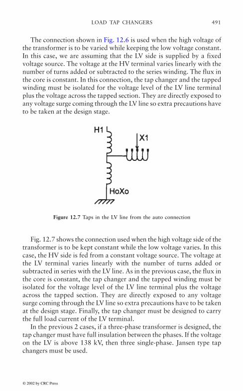
491LOAD TAP CHANGERS
The connection shown in Fig. 12.6 is used when the high voltage ofthe transformer is to be varied while keeping the low voltage constant.In this case, we are assuming that the LV side is supplied by a fixedvoltage source. The voltage at the HV terminal varies linearly with thenumber of turns added or subtracted to the series winding. The flux inthe core is constant. In this connection, the tap changer and the tappedwinding must be isolated for the voltage level of the LV line terminalplus the voltage across the tapped section. They are directly exposed toany voltage surge coming through the LV line so extra precautions haveto be taken at the design stage.
Fig. 12.7 shows the connection used when the high voltage side of thetransformer is to be kept constant while the low voltage varies. In thiscase, the HV side is fed from a constant voltage source. The voltage atthe LV terminal varies linearly with the number of turns added orsubtracted in series with the LV line. As in the previous case, the flux inthe core is constant, the tap changer and the tapped winding must beisolated for the voltage level of the LV line terminal plus the voltageacross the tapped section. They are directly exposed to any voltagesurge coming through the LV line so extra precautions have to be takenat the design stage. Finally, the tap changer must be designed to carrythe full load current of the LV terminal.
In the previous 2 cases, if a three-phase transformer is designed, thetap changer must have full insulation between the phases. If the voltageon the LV is above 138 kV, then three single-phase. Jansen type tapchangers must be used.
Figure 12.7 Taps in the LV line from the auto connection
© 2002 by CRC Press

LOAD TAP CHANGERS492
The connection shown in Fig. 12.8 can be used when the LV is to bevaried while the HV is to be kept constant. The advantages of thisconnection are:
• The level of insulation for the tapped winding and the tap changeris low
• A Wye connected three-phase tap changer can be used for a three-phase transformer
• The current in the common winding is lower than the current inthe LV line terminal; so a smaller tap changer can be selected.
As usual, there is a price to pay to obtain these benefits. If we assumethat the voltage between H1 and HoXo is constant, varying the numberof turns implies varying the volts/turn, and therefore the flux in thecore. It is a variable flux design. As explained earlier, in a variableflux transformer, the losses, the exciting current, the impedance, and thesound level vary with the tap position, and a bigger core must be selectedfor proper operation at the minimum turn position. If there is a tertiarywinding, its voltage will vary as the tap changer changes position.
In an auto-transformer connection, the turns in the common branchare part of both the HV and LV circuits. This means that if we add turnsin the common branch, we add turns to both the HV and LV circuits.Because of this, the number of turns required to achieve a specifiedregulating range is higher than for the other 2 cases. Here is anexample.
Figure 12.8 Taps in the common winding of an autotransformer, at the neutral end
© 2002 by CRC Press

493LOAD TAP CHANGERS
Let us suppose that we want 10% voltage regulation. We need aratio that varies by 10% when we add all the turns of the tappedwinding. Suppose that we have 100 turns in the series winding and 100turns in the common winding. The LV circuit has 100 turns and the HVcircuit has 200 turns with no taps in circuit. It gives a ratio of 2:1. Let usconsider all three cases:
1) For the tapped turns in the series winding, if we want a 10%change in the HV, we need to add or remove 20 turns to the HVcircuit. The size or rating of the tapped winding would be 10% ofthe HV x the full load current of the HV=10% of the total MVA ofthe transformer.
2) For the case of taps in the LV line from the auto point, we need toadd or remove 10 turns to the LV circuit to achieve 10% change inthe LV. The size of the winding would be 10% of the LV voltage xthe full current of the LV=10% of the total MVA of the transformer.The ratio of LV to HV is 0.5 +/-.05 or 0.45-0.55
3) In the case of the taps in the neutral end, assuming that the HV isconstant, in order to increase the LV by 10%, we needapproximately 23 turns in order to get a ratio of 123/223= 0.552.If we subtract the 23 turns (we add them in reverse polarity), weobtain a ratio of 77/177=0.435. The variation of the voltage is notsymmetrical. The size of the tapped winding is 23% of the commonwinding or 11.5% of the total MVA of the transformer. It is biggerthan the other 2 cases and the volts per step in the tap changer isalso higher. The designer of the transformer has to weigh all thesefactors when selecting the connection of the tap winding.
12.5.3 Use of Auxiliary Transformer
When a transformer with a relatively high current LV winding is specifiedand regulation is desired on the LV side, it may be economical to use anauxiliary transformer to achieve regulation. This gives the designer agreater flexibility in the design of the tapped winding and the savingson the main transformer often outweighs the cost of the auxiliarytransformer. There are 2 popular way of using auxiliary transformers.
The Series Voltage Regulator
In this connection, the tapped winding is located on the auxiliarytransformer which is inserted in series with the low voltage line terminal,
© 2002 by CRC Press

LOAD TAP CHANGERS494
The Series (booster) Transformer
In this connection, shown in Fig. 12.10, the tapped winding is a separatewinding on the main transformer. The advantages of this connectionare that there is much more flexibility in the design of the tapped winding.The number of turns per step can be selected so that the tap changercarries a smaller current. The main saving in this case is on the tapchanger itself and in the greater flexibility in the optimization of themain transformer.
adding or subtracting its voltage with the LV winding of the maintransformer. The main transformer has only 2 windings and can beoptimized independently from the series voltage regulator (SVR). Thisis shown in Fig. 12.9.
Figure 12.9 Tap changing scheme using a series voltage regulator
Figure 12.10 Tap changing scheme using a series (booster) transformer
Auxiliary transformers can also be used with auto-transformerspretty much in the same way. There are also plenty of possibleconnections for using auxiliary transformers. The choice is only limitedby the imagination of the designer.
© 2002 by CRC Press

495LOAD TAP CHANGERS
12.5.4 Phase shifting transformers
A phase shifting transformer is ideally a transformer with a 1:1 voltageratio and which has the ability to change the phase angle of its outputvoltage relative to its input. This feature is used by electric powercompanies to help transfer power more efficiently within the electricalgrid. In these transformers, the voltage from the tapped windings isadded in quadrature with the input line terminals, producing an effectivephase shift in the output. There are quite a few possible connections toachieve this and some of these are discussed in Chapter 13. Let us justmention here that in a phase shifting transformer, the tap changer is akey element and the size and rating of the tapped windings are muchhigher than for conventional transformers.
12.6 GENERAL MAINTENANCE
The reason for the maintenance on a tap changer is to insure its reliability.Any device with moving parts, some of which are used to interruptcurrents and voltages requires maintenance. It would be useless to repeathere what can be found in the manufacturers instruction books. We willonly mention general principles. The factors affecting the reliability oftap changers include:
• Oil quality• Contact pressure• Contact resistance and temperature• Timing of movements• Load currents• Number of operations
The maintenance of the controls and the drive mechanism are normallynot a problem. The gears and other moving parts might wear and requirereplacement, but in general, they are designed to last very long and donot need frequent inspection. The main areas of concern are the switchesand the connecting board if present. The contacts have to be inspectedand verified periodically. The frequency of these inspections dependsmainly on the number of operations, the current flowing through thecontacts and the cleanliness of the oil.
The inspection and replacement of contacts require that thetransformer be taken out of service. Since it is always costly to take a
© 2002 by CRC Press

LOAD TAP CHANGERS496
transformer out of service, it is desirable to extend the period betweeninspections as much as possible. Besides recommendations that can befound in most instruction books for tap changers, here are some of thetactics used by utilities to reduce their maintenance costs and the failurerate of their tap changers.
The process of changing tap position includes arcing, whichgenerates gases and carbon particles. The movement of contacts alsopromotes erosion of the metal and generates small metal particles. Inthe long run, these particles can affect the dielectric properties of the oil.Moreover, the carbon particles tend to aggregate on contacts andincrease the contact resistance. They also accumulate on connectingboards and may lead to tracking on the surface of the board. For thesereasons, the reliability of a tap changer and its overall performance canbe improved by a simple filtering device which would keep the oilclean. This is specially important if the arcing switch is located in thesame compartment as the selector and change-over switches. Someutilities have introduced oil filters for load tap changers and they havefound that with these filters, they can extend their time betweeninspections. However in some tap changers, the arcing occurs in aseparate vacuum chamber so that oil comtamination is reduced oreleminated.
In a tap changer, contacts that operate frequently remain clean. Theones that do not move tend to oxidize or collect carbon or both. Withtime, their contact resistance increases, which produces more heat andthe situation deteriorates. This is typical of change-over selectors. Someof those operate only twice a year. Many cases of damage to theseswitches have been reported. Several utilities now force their tapchangers to ride over the mid position at least once a month and theyclaim a much better performance of their tap changers since they haveintroduced the procedure.
Instead of taking all transformers out of service for regular andfrequent inspections of tap changers, some utilities have introducedmonitoring procedures for tap changers without de-energizing theirtransformers. One of those procedures is dissolved gas analysis (DGA).They regularly take oil samples from tap changer compartments andmonitor the gasses. After a while, they know the pattern of all their tapchangers. Whenever one changes pattern, they go and inspect it. Theyreport that this procedure has helped them reduce the frequency of theirinternal inspections while alerting them to dangerous problems beforethey lead to a catastrophic failure.
© 2002 by CRC Press

497LOAD TAP CHANGERS
Another trick is to have inspection windows in the tap changer box.When used in conjunction with an oil filter, they can look at theircontacts without opening the box and take the transformer out ofservice if required.
Another possible procedure is to monitor the temperature on the tapchanger compartment regularly with infrared measuring devices. It isvery inexpensive and easy to do. They claim that if anything goeswrong in a tap changer, it typically increases the temperature of thecontacts to a point that you can detect it by checking the temperature onthe outside of the wall of the box. Their rule is that if the temperature onthe surface of the tap changer compartment is higher than the tank ofthe transformer by more than 7 to 10 degrees, something is going wronginside the transformer. They would then inspect the tap changer. Quitea few problems have been detected this way.
© 2002 by CRC Press

499
13. PHASE SHIFTINGTRANSFORMERS
Summary Equivalent circuit models are derived for three commonlyused types of phase shifting transformer. The winding configurationsare chosen to have a positive phase shift and no change in voltagemagnitude at no-load. The equivalent impedance as seen from the inputor output is expressed in terms of two winding impedances. This is donefor positive, negative, and zero sequence circuits. Negative sequencecircuits have a negative phase shift and zero sequence circuits have nophase shift. The model is then used to study regulation effects and tocalculate fault currents for the major fault types.
13.1 INTRODUCTION
Phase shifting transformers are used in power systems to help controlpower flow and line losses. They shift the input voltage and currentphases by an angle which can be adjusted by means of a tap changer.They operate by adding a voltage at ±90° to the input voltage, i.e. inquadrature. For 3 phase transformers, the quadrature voltage to be addedto a given phase voltage can be derived from the other phases. Themany ways of doing this give rise to a large number of configurationsfor these transformers. We will deal with only a few common typeshere. Phase shifting capability can be combined with voltage magnitudecontrol in the same transformer. This results in a more complex unit,involving two sets of tap changers, which we no not discuss here.
As a simplified example of their utility, consider the circuit in Fig.13.1 where a power source at voltage V is feeding a load along twoparallel paths. (We use bold faced symbols for phasor quantities.) Withthe voltage source E=0, the currents will divide according to the lineimpedances Z1 and Z2,
(13.1)
© 2002 by CRC Press

PHASE SHIFTING TRANSFORMERS500
With E inserted, we find,
(13.2)
Since, normally , the efifect of E is to add a current to I2
and subtract a current from I1, i.e. introduce a circulating current of
(13.3)
The magnitude as well as the phase of E controls the amount of circulatingcurrent.
Figure 13.1 Addition of voltage E to control circulating current
In the approximation that ZL is much larger than Z1 or Z2 andassuming Z1=Z2=Z, we have
(13.4)
© 2002 by CRC Press
PHASE SHIFTING TRANSFORMERS 501
If ZL is resistive, i.e. a unity power factor load, and Z is primarilyinductive or capacitive, then
(13.5)
Thus if E is ±90° out of phase with V, then a circulating current in phasewith the primary current results. This can be useful in controlling theflow of real power along each of the parallel lines. A phase shiftingtransformer could add the required E.
As another example, consider feeding a common load from twovoltage sources which could be out of phase with each other as shown inFig. 13.2 Solving for the currents, we get
(13.6)
The current into the load. IL, is
(13.7)
and the voltage across the load, VL, is
(13.8)
Thus the complex power delivered to the load is
(13.9)
where * denotes complex conjugation.
© 2002 by CRC Press

PHASE SHIFTING TRANSFORMERS502
Consider the case where Z1=Z2=Z. V1=V. V2=Vejθ. Then (13.9)becomes
(13.10)
Thus it can be seen that the maximum power is transferred when θ=0, Inthis case a phase shifting transformer could be used to adjust the phaseof V2 so that it equals that of V1.
In modern power systems which are becoming more and moreinterconnected, the need for these devices is growing. Other methods forintroducing a quadrature voltage are being developed, for instance bymeans of power electronic circuits in conjunction with ac-dc converters,These can act much faster than on-load tap changers. However, atpresent they are more costly than phase shifting transformers and areused primarily when response time is important. (Electronic on-load tapchangers are also being developed for fast response time applications.)
In this report, we develop a circuit model description for threecommon types of phase shifting transformer. This is useful in order tounderstand the regulation behavior of such devices, i.e. how much theoutput voltage magnitude and phase change when the unit is loaded ascompared with the no load voltage output. In the process, we also findhow the phase angle depends on tap position, a relationship which canbe non-linear. In addition to the positive sequence circuit model whichdescribes normal operation, we also determine the negative and zerosequence circuit models for use in short circuit fault current analysis.
Figure 13.2 Two possibly out of phase sources feeding a common load
© 2002 by CRC Press

PHASE SHIFTING TRANSFORMERS 503
The latter analysis is carried out for the standard types of fault for twoof the phase shifting transformers.
Very little has been published on this subject in the open literaturebeyond general interconnection diagrams and how they are used inspecific power grids. However, several references which emphasizebasic principles are Refs.[Hob39. Cle39]. Other useful references are[Kra98, Wes64].
13.2 BASIC PRINCIPLES
We neglect exciting current and model the individual phases in terms oftheir leakage impedances. For a two winding phase, we use the circuitmodel shown in Fig. 13.3. Z12 is the two winding leakage impedancereferred to side 1. Most of the development described here is carried outin terms of impedances in Ohms. Because of differences in per unitbases for the input and winding quantities, per unit quantities are not asconvenient in the analysis. At the appropriate place, we indicate whereper unit quantities might prove useful. The currents are assumed to flowinto their respective windings. With N1 the number of turns on side 1and N2 the number of turns on side 2, the ideal transformer voltagessatisfy
(13.11)
and the currents satisfy
(13.12)
© 2002 by CRC Press

PHASE SHIFTING TRANSFORMERS504
For 3 windings per phase, we use the model shown in Fig. 13.4. Inthis case, the ideal transformer voltages satisfy
(13.13)
and the currents satisfy
N1I1+N2I2+N3I3=0 (13.14)
The single winding impedances are given in terms of the 2 windingimpedances by
(13.15)
Here the two winding impedances are referred to the windingcorresponding to the first subscript and the second subscript refers to the
Figure 13.3 Model of a two winding transformer phase
© 2002 by CRC Press
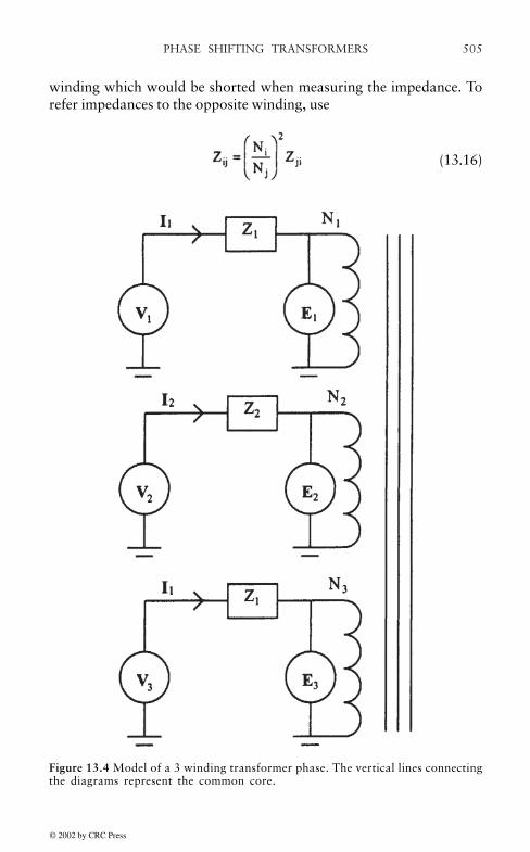
PHASE SHIFTING TRANSFORMERS 505
winding which would be shorted when measuring the impedance. Torefer impedances to the opposite winding, use
(13.16)
Figure 13.4 Model of a 3 winding transformer phase. The vertical lines connectingthe diagrams represent the common core.
© 2002 by CRC Press

PHASE SHIFTING TRANSFORMERS506
For a 3 phase system, the positive sequence quantities correspond tothe ordering of the unit phasors shown in Fig. 13.5. Letting
(13.17)
the ordering is 1, α2, α. Negative sequence ordering is 1, α, α2. This isobtained by interchanging 2 phases. Note that
(13.18)
Zero sequence quantities are all in phase with each other.
Figure 13.5 Positive sequence unit phasors
Our interconnections will be chosen to produce a positive phase shiftat a positive tap setting. By interchanging two phases, a negative phaseshift can be produced at a positive tap setting. Interchanging two phasesis equivalent to imputing a negative sequence set of voltages. Thisimplies that negative sequence circuits have the opposite phase shift topositive sequence circuits. Zero sequence circuits have zero phase shift.By positive phase shift we mean that output voltages and currents leadinput voltages and currents, i.e. output quantities are rotated counterclockwise on a phasor diagram relative to input quantities.
© 2002 by CRC Press

PHASE SHIFTING TRANSFORMERS 507
13.3 SQUASHED DELTA PHASE SHIFTING TRANSFORMER
One of the simplest phase shifters to analyze is the squashed deltaconfiguration shown in Fig. 13.6. In the figure S labels the source orinput quantities and L the load or output quantities. The input andoutput set of voltages and corresponding currents form a balanced positivesequence set. The input and output voltage phasor diagram is shown inFig 13.6b. These are voltages to ground. The currents form a similar setbut are not shown. Similarly, the internal voltages and correspondingcurrents form a positive sequence set as shown in Fig. 13.6c for thevoltages. Note that Figs 13.6b and 13.6c could be rotated relative toeach other if shown on a common phasor diagram. Information on theirrelative orientation is not contained in the figure although the phaseorder is consistent between the figures. This applies as well to thecorresponding current phasors. a and a', etc. refer to windings on thesame leg, with the prime labeling the tapped winding. The 2 windingimpedances will be referred to the unprimed coil, i.e. etc. Since theseimpedances are all the same by symmetry, we need only this one symbol.This transformer can be designed with a single 3 phase core and isreferred to genetically as a single core design. It is also best adapted tophase angle shifts in one direction.
© 2002 by CRC Press
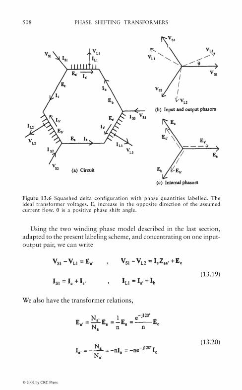
PHASE SHIFTING TRANSFORMERS508
Using the two winding phase model described in the last section,adapted to the present labeling scheme, and concentrating on one input-output pair, we can write
(13.19)
We also have the transformer relations,
(13.20)
Figure 13.6 Squashed delta configuration with phase quantities labelled. Theideal transformer voltages. E, increase in the opposite direction of the assumedcurrent flow. θ is a positive phase shift angle.
© 2002 by CRC Press

PHASE SHIFTING TRANSFORMERS 509
where we have defined , the turns ratio. We also have thefollowing relationships,
(13.21)
It is worthwhile going into the details of the solution of these equationssince we will need some of the intermediate results later. We assumethat VS1 and IS1 are given. From (13.19) and (13.20), we obtain
(13.22)
We also have
(13.23)
where
Since n is determined by the tap position, this shows that θ is a non-linear function of the tap position, assuming the taps are evenly spaced.
Adding equations (13.21) and using (13.19),
Solving for Ec, using (13.22),
(13.24)
© 2002 by CRC Press

PHASE SHIFTING TRANSFORMERS510
Combining with the first of equations (13.19) and (13.20), we obtain
(13.25)
where θ is given in (13.23). Although the current is shifted by θ in allcases, in general, the voltage is shifted by θ only under no load conditions.
The circuit model suggested by (13.25) is shown in Fig. 13.7. Bysymmetry, this applies to all three phases with appropriate labeling.The equivalent impedance shown in Fig. 13.7 is given by
(13.26)
Fig. 13.7 is a positive sequence circuit model. The negative sequencemodel is obtained simply by changing to -θ with Zeq unchanged. Notethat Zeq depends on the tap setting.
Figure 13.7 Circuit model of one phase of a phase shifting transformer This is forpositive sequence. For negative sequence, change θ to -θ.
While the input power per phase is Pin=VS1IS1*, the transformed or
winding power per phase. Pwdg, is somewhat less. Ignoring impedancedrops, we have from (13.22) and (13.24),
(13.27)
© 2002 by CRC Press
PHASE SHIFTING TRANSFORMERS 511
where the factor of j shows that the transformed power is in quadraturewith the input power. As a numerical example, let θ=30°. Then, from(13.23) and (13.27),
We can express (13.25) in per unit terms, however because of thedifference between the input power and voltage base and that of thewindings, we must be careful to specify the base used. For the inputbase, use the rated input power. Pin,b, the rated input voltage. Vin,b, andthe rated input current which can be derived from the power andvoltage base. Iin,b=Pin,b/Vin,b. Similarly the input impedance base can bederived from the power and voltage base. Zin,b=Vin,b/Iin,b=(Vin,b)2/Pin,b.Note that, because the transformation ratio is 1:1 in terms ofmagnitude, the output base values are the same as the input basevalues. Thus (13.25) can be written
(13.28)
where small letters are used to denote per unit quantities. Note that allthe quantities in (13.28) are on a consistent base.
However, it is often more convenient to express winding quantitiessuch as impedances on a winding basis. Assuming rated input powerand voltage, the winding impedance base can be obtained from (13.27)and (13.24), ignoring impedance drops,
(13.29)
Thus. Zeq can be expressed as
(13.30)
© 2002 by CRC Press
PHASE SHIFTING TRANSFORMERS512
where, as the development in (13.30) indicates, zeq is on an input baseand is on a winding base. Note that the winding base depends on the
turns ratio as indicated in (13.29). Thus this base is perhaps most usefulwhen n refers to the maximum phase angle. At the other extreme, withθ=0, we have n=, so that Zeq=Zeq=0. In this case, the input is directlyconnected to the output, bypassing the coils.
The zero sequence circuit model may be derived with reference toFig. 13.6 but assuming all quantities are zero sequence. Thus Fig.13.6b, c should be replaced by diagrams with all phasors in parallelUsing a zero subscript for zero sequence quantities, we can write
(13.31)
and
(13.32)
Since Ib,0=Ic,0, (13.31) shows that
IL1,0=IS1,0 (13.33)
so the current is not phase shifted. We also have
(13.34)
Solving the above zero sequence equations, we obtain
(13.35)
and
© 2002 by CRC Press

PHASE SHIFTING TRANSFORMERS 513
(13.36)
The circuit model for this last equation is shown in Fig. 13.8, where wehave defined
(13.37)
This has a different dependence on n from the positive sequence circuit.It becomes infinite when n=1. This is reasonable, because from (13.32)
when n=1 so that from (13.31) IS1,0=0. Thus no zero sequencecurrent can flow into the squashed delta transformer when n=1. Internalcurrent can however circulate around the delta. From (13.23), θ=60°when n=1.
Figure 13.8 Zero sequence circuit model of one phase of a squashed delta phaseshifting transformer
There is no phase angle shift in the voltage at no load. Equation(13.36) can be written in per unit terms referred to the same input baseas used for positive sequence
vL1,0=vS1,0-iS1,0zeq,0 (13.38)
Using the positive sequence winding base for the two winding zerosequence impedance, we can write
© 2002 by CRC Press

PHASE SHIFTING TRANSFORMERS514
(13.39)
As before, in (13.39), the two z’s are on different bases and this expressionis primarily useful when the winding base is for the maximum phaseshift angle,
We postpone a discussion of regulation effects and short circuitcurrent calculations until other types of phase shifting transformers aretreated. This is because the positive, negative, and zero sequence circuitdiagrams for all the cases treated will have the same appearance,although Zeq or zeq and θ will differ among the various types.
13.4 STANDARD DELTA PHASE SHIFTING TRANSFORMER
As opposed to the squashed delta design, the standard delta design utilizesan unsquashed delta winding but is still a single core design. Theconnection diagram is given in Fig. 13.9. The tapped windings are onthe same core as the corresponding parallel windings on the delta in thefigure. The taps are symmetrically placed with respect to the point ofcontact at the delta vertex. This assures that there is no change in currentor no-load voltage magnitude from input to output. It also means that
, etc. for the other phases. Each phase really consists of threewindings, the two tap windings and the winding opposite and parallelin the figure, where primes and double primes are used to distinguishthem. Thus a 3 winding per phase model is needed. will beused to label the single winding impedances for phase a. Since all thephases have equivalent impedances by symmetry, these samedesignations will be used for the other phases as well. The same remarksapply to the phasor diagrams as for the squashed delta case. Althoughnot shown, the current phasor diagrams have the same sequence orderas their corresponding voltage phasor diagrams, however the twodiagrams could be rotated relative to each other.
In Fig. 13.9a, V1, V2, V3 designate the phasor voltages to ground atthe delta vertices. Thus we have, using , etc. and
, etc.,
© 2002 by CRC Press

PHASE SHIFTING TRANSFORMERS 515
(13.40)
In addition, we have the transformer relations
(13.41)
where we have defined the turns ratio n as the ratio between the turns inone of the delta windings to the turns in one of the tap windings. Bothtap windings have the same number of turns. Solving for Ia in the lastequation in (13.40) and inserting into the last equation in (13.41), weobtain
(13.42)
We also have
(13.43)
© 2002 by CRC Press

PHASE SHIFTING TRANSFORMERS516
Figure 13.9 Standard delta configuration with phase quantities labelled. Theideal transformer voltages. E, increase in the opposite direction of the assumedcurrent flow. The taps are symmetrically positioned.
© 2002 by CRC Press

PHASE SHIFTING TRANSFORMERS 517
From the above equations, we obtain
(13.44)
and
(13.45)
with θ as given in (13.42). This is the no-load phase angle shift. Thisconforms to the circuit model shown in Fig. 13.7 with
(13.46)
or in terms of 2 winding impedances, using (13.15),
(13.47)
This is the positive sequence circuit. As before the negative sequencecircuit is found by changing θ to -θ without change in Zeq.
Let us again determine the winding power per phase. Pwdg, in terms ofthe input power per phase. Pin=VS1IS1*. Again, ignoring impedancedrops, we get
(13.48)
where j indicates that the transformed power is in quadrature with theinput power. Using trigonometric identities, it can be shown that
Pwdg=jsinθPin (13.49)
© 2002 by CRC Press
PHASE SHIFTING TRANSFORMERS518
with as given in (13.42). (This relation does not hold for the squasheddelta design.) Thus for θ=30°, |Pwdg|=0.5|Pin|. In per unit terms, based oninput quantities, (13.45) can be cast in the form of (13.28). If we wish touse a winding base for the 2 winding impedances given in (13.47) thenwe must determine the relation between their bases and the input basefor impedances. The 2 winding impedances given above are referred toeither the a or a' winding. Their bases are given by.
(13.50)
Thus, in per unit terms. Zeq in (13.47) becomes
(13.51)
As before zeq is on an input base and the 2 winding impedances on theirwinding base. Again this is primarily useful when n refers to the maximumphase angle. At zero phase shift, n=, (13.47) indicates that .However, at this tap position, the tap windings are effectively out of thecircuit so that and the input is directly connected to the output.
The zero sequence circuit model can be derived with reference to Fig.13.9 but with all phasors taken to be zero sequence. Rewriting (13.40)and (13.41) with this in mind and appending a zero subscript, we get
(13.52)
Solving, we find
IL1,0=IS1,0 (13.53)
© 2002 by CRC Press

PHASE SHIFTING TRANSFORMERS 519
so that the zero sequence current undergoes no phase shift. We also have
(13.54)
and
(13.55)
Thus the voltage undergoes no phase shift at no-load. The circuitmodel of Fig. 13.8 applies with
(13.56)
or, in terms of 2 winding impedances,
(13.57)
On a per unit basis, using rated input quantities, (13.55) has the sameappearance as (13.38). The equivalent per unit impedance on an inputbase with the 2 winding impedances on their positive sequence windingbases is given by
(13.58)
Again this is primarily useful when n refers to the maximum phaseangle shift. At zero phase shift, the output is directly connected to theinput as was the case for positive sequence,
13.5 TWO CORE PHASE SHIFTING TRANSFORMER
For large power applications, phase shifters are often designed as twounits, the series unit and the excitor unit, each having its own core andassociated coils. Depending on size, the two units can be inside thesame tank or be housed in separate tanks. This construction is largely
© 2002 by CRC Press
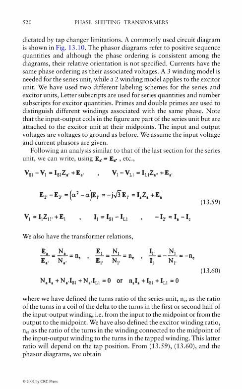
PHASE SHIFTING TRANSFORMERS520
dictated by tap changer limitations. A commonly used circuit diagramis shown in Fig. 13.10. The phasor diagrams refer to positive sequencequantities and although the phase ordering is consistent among thediagrams, their relative orientation is not specified. Currents have thesame phase ordering as their associated voltages. A 3 winding model isneeded for the series unit, while a 2 winding model applies to the excitorunit. We have used two different labeling schemes for the series andexcitor units, Letter subscripts are used for series quantities and numbersubscripts for excitor quantities. Primes and double primes are used todistinguish different windings associated with the same phase. Notethat the input-output coils in the figure are part of the series unit but areattached to the excitor unit at their midpoints. The input and outputvoltages are voltages to ground as before. We assume the input voltageand current phasors are given.
Following an analysis similar to that of the last section for the seriesunit, we can write, using , etc.,
(13.59)
We also have the transformer relations,
(13.60)
where we have defined the turns ratio of the series unit, ns, as the ratioof the turns in a coil of the delta to the turns in the first or second half ofthe input-output winding, i.e. from the input to the midpoint or from theoutput to the midpoint. We have also defined the excitor winding ratio,ne, as the ratio of the turns in the winding connected to the midpoint ofthe input-output winding to the turns in the tapped winding. This latterratio will depend on the tap position. From (13.59), (13.60), and thephasor diagrams, we obtain
© 2002 by CRC Press

PHASE SHIFTING TRANSFORMERS 521
which implies
(13.61)
Figure 13.10 Circuit diagram of a 2 core phase shifting transformer. The idealtransformer voltages, the E’s, increase in the opposite direction to the assumedcurrent flow. The input-output coil is equally divided.
© 2002 by CRC Press
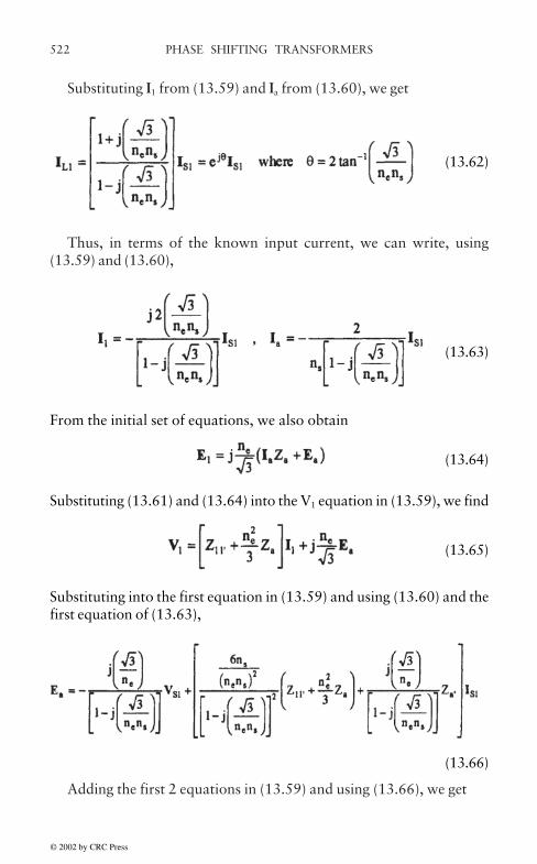
PHASE SHIFTING TRANSFORMERS522
Substituting I1 from (13.59) and Ia from (13.60), we get
(13.62)
Thus, in terms of the known input current, we can write, using(13.59) and (13.60),
(13.63)
From the initial set of equations, we also obtain
(13.64)
Substituting (13.61) and (13.64) into the V1 equation in (13.59), we find
(13.65)
Substituting into the first equation in (13.59) and using (13.60) and thefirst equation of (13.63),
(13.66)
Adding the first 2 equations in (13.59) and using (13.66), we get
© 2002 by CRC Press

PHASE SHIFTING TRANSFORMERS 523
(13.67)
where θ is given in (13.62). This can be represented with the samecircuit model as Fig. 13.7, with
(13.68)
or, in terms of 2 winding impedances,
(13.69)
Using (13.63) and (13.64) and ignoring impedance drops, we can showthat the winding power per phase is the same for the series and excitorunits, i.e.,
(13.70)
In terms of the phase shift θ given in (13.62), (13.70) can be written
Pwdg=jsinθPin (13.71)
as was the case for the standard delta phase shifter.In per unit terms, based on rated input power and voltage, (13.67)
can be cast in the form of (13.28). To express the two windingimpedances on their winding bases, we need to find the impedancewinding bases for both the series and excitor windings. Although thewinding power is the same for these, their voltages are different. Usingthe above formulas, we find
© 2002 by CRC Press

PHASE SHIFTING TRANSFORMERS524
(13.72)
Using these relations, the per unit equivalent impedance can be written
(13.73)
where as before zeq is on an input base and the two winding impedancesare on their winding bases. Again this is primarily useful when ne refersto the maximum phase angle shift. Also the negative sequence circuithas the same equivalent impedance but a phase angle shift in the oppositedirection to the positive sequence circuit.
The zero sequence circuit model is derived with reference to Fig.13.10 by assuming all quantities are zero sequence. Thus we simplyrewrite the basic equations, appending a zero subscript,
(13.74)
and
(13.75)
Solving, we find,
© 2002 by CRC Press

PHASE SHIFTING TRANSFORMERS 525
(13.76)
Notice that, even if both Y windings of the excitor were grounded, nozero sequence current flows into the excitor because the secondary currentfrom the tap winding would have to flow into the closed delta of theseries unit and this is not possible for zero sequence currents.
From the above formulas, we obtain
(13.77)
Thus we see that the zero sequence current and no-load voltage have nophase angle shift and the circuit of Fig. 13.8 applies with
(13.78)
or, in terms of 2 winding impedances,
(13.79)
Using the same basis as for positive sequence, the per unit version of(13.79) is
(13.80)
where, as before, zeq,0 is on an input base and the two winding impedancesare on their winding bases.
© 2002 by CRC Press
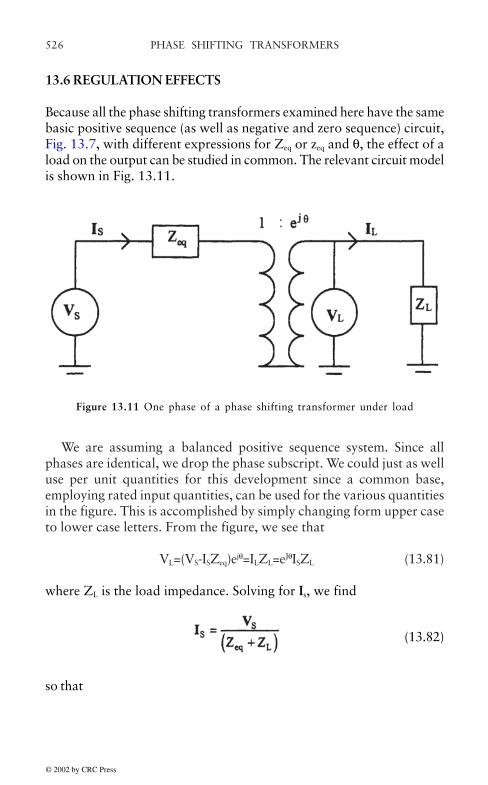
PHASE SHIFTING TRANSFORMERS526
13.6 REGULATION EFFECTS
Because all the phase shifting transformers examined here have the samebasic positive sequence (as well as negative and zero sequence) circuit,Fig. 13.7, with different expressions for Zeq or zeq and θ, the effect of aload on the output can be studied in common. The relevant circuit modelis shown in Fig. 13.11.
We are assuming a balanced positive sequence system. Since allphases are identical, we drop the phase subscript. We could just as welluse per unit quantities for this development since a common base,employing rated input quantities, can be used for the various quantitiesin the figure. This is accomplished by simply changing form upper caseto lower case letters. From the figure, we see that
VL=(VS-ISZeq)ejθ=ILZL=eJθISZL (13.81)
where ZL is the load impedance. Solving for Is, we find
(13.82)
so that
Figure 13.11 One phase of a phase shifting transformer under load
© 2002 by CRC Press

PHASE SHIFTING TRANSFORMERS 527
(13.83)
Thus any phase angle or magnitude shift from no load conditions isdue to a non-zero Zeq/ZL. Since Zeq is almost entirely inductive, a purelyinductive or capacitive load will not affect θ but will result only in amagnitude change in the voltage. On the other hand, a resistive orcomplex load will lead to both magnitude and phase angle shifts.
Following convention, let the load current lag the load voltage by anangle θL, i.e. if θV is the voltage phasor angle, then
(13.84)
Note the distinction between bold faced phasor quantities and normaltype used for magnitudes in the above equation. A positive value of θL ischaracteristic of a load with an inductive component. Let us also set
Zeq=R+jX (13.85)
Then
(13.86)
Under no-load. NL, conditions (ZL=), (13.83) shows that
VL,NL=VSejθ
Thus taking ratios and using (13.86), we see that
(13.87)
© 2002 by CRC Press

PHASE SHIFTING TRANSFORMERS528
Thus the presence of a load will lower the magnitude and shift the phasegenerally in a negative direction since R is usually small comparedwith X and θL is generally positive and closer to zero that to 90°.
13.7 FAULT CURRENT ANALYSIS
We briefly review the sequence circuit method of fault current analysishere. This will also help establish notation. Although we do not workon a per unit basis, the same formulas apply with the substitution oflower case letters for the upper case ones if the input base is used. Ourphase designations here are not necessarily related to those chosen forthe transformers previously analyzed. Let Vfa, Vfb, Vfc be the voltages atthe fault point for phases a, b, c and let the currents leaving the fault beIfa, Ifb, Ifc. These voltages and currents do not necessarily form a balancedset. The positive, negative, and zero sequence phasors corresponding tophase a will be denoted Vfa,1, Vfa,2, Vfa,0 and Ifa,1, Ifa,2, Ifa,0 respectively.Each one of these has a corresponding member for phases b and c sothat Vfa,1, Vfb,1, Vfc,1 form a balanced positive sequence set, Vfa,2, Vfb,2,Vfc,2 form a balanced negative sequence set, and Vfa,0, Vfb,0, Vfc,0 form abalanced zero sequence set. Therefore, once Vfa,1 is known, Vfb,1 and Vfc,1
are automatically determined and similarly for Vfa,2 and Vfa,0—The sameapplies to currents. Thus Vfa,1, Vfa,2, Vfa,0 contain all the informationavailable in the original set Vfa, Vfb, Vfc. It is therefore natural that theyare related by some transformation. This is given by
(13.88)
and its inverse
(13.89)
where α is given in (13.17). The above equations also apply to currentswith appropriate change in notation.
© 2002 by CRC Press

PHASE SHIFTING TRANSFORMERS 529
Since the sequence systems are balanced systems, it is only necessaryto study one phase of each system. Quite generally, they can bemodeled as a Thevenin equivalent system, containing an ideal voltagesource in series with a Thevenin equivalent impedance as shown in Fig.13.12. A voltage source is shown only in the positive sequence circuitsince 3 phase sources are generally positive sequence.
From Fig. 13.12, we have
Vfa,1=ET-Ifa,1ZT1, Vfa,2=-Ifa,2ZT2, Vfa,0=-Ifa,0ZT0 (13.90)
The faults of interest are:
(1) 3 phase line to ground fault(2) Single phase line to ground fault(3) Line to line fault(4) Double line to ground fault
For fault type (1), we have Vfa=Vfb=Vfc=0 so that, using (13.88) –(13.90),
(13.91)
This simply means that the fault currents form a balanced positivesequence set as expected from the symmetry of the fault.
For fault type (2), we assume that the a phase line is shorted so thatVfa=0, Ifb=Ifc=0. From (13.88)–(13.90),
Figure 13.12 Thevenin equivalent swquence circuits
© 2002 by CRC Press

PHASE SHIFTING TRANSFORMERS530
(13.92)
For fault type (3), assume the b and c lines are shorted together sothat Vfb=Vfc, Ifa=0. Ifc=”Ifb. From (13.88)–(13.90), we obtain
(13.93)
For fault type (4), we assume the b and c lines are shorted to groundso that Vfb=Vfc=0. Ifa=0. Then from (13.88)–(13.90),
(13.94)
Because voltages and currents are untransformed in magnitude andtransformed by the same phase shift across the ideal transformer in Fig.13.7, impedances can be brought to one side or the other of the circuitwithout change. We make use of this fact by shifting system impedanceson the load side to the source side and consider faults at the sourceterminal. Faults on the load side can be found from the source sideresults by slight notational changes in the results. Thus the sequencecircuit diagrams shown in Fig. 13.13 can be used. ZSS and ZSL aresystem impedances on the source and load sides respectively. Note thatEout is the load voltage multiplied by e”jθ to bring it across the idealtransformer. Positive and negative sequence impedances are notdistinguished with subscripts since they are the same to a goodapproximation.
© 2002 by CRC Press
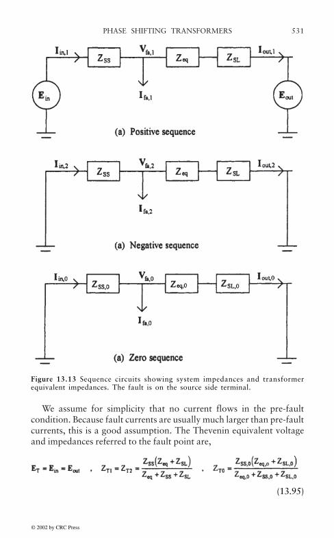
PHASE SHIFTING TRANSFORMERS 531
We assume for simplicity that no current flows in the pre-faultcondition. Because fault currents are usually much larger than pre-faultcurrents, this is a good assumption. The Thevenin equivalent voltageand impedances referred to the fault point are,
(13.95)
Figure 13.13 Sequence circuits showing system impedances and transformerequivalent impedances. The fault is on the source side terminal.
© 2002 by CRC Press

PHASE SHIFTING TRANSFORMERS532
By substituting these into previous formulas, we obtain the faultsequence currents in terms of known quantities. The fault sequencecurrents into the transformer source side terminal are Iout,1 , Iout,2 , Iout,0.From Fig. 13.13, (13.90) and ZT1=ZT2, we obtain
(13.96)
This last set of equations are standard equations for fault currentsinto a two winding transformer. However, in a phase shiftingtransformer, the winding currents are quite different from the terminalcurrents. In addition, positive and negative sequence currentsexperience opposite phase shifts. This makes the analysis of faultcurrents inside these transformers quite different from fault currents in astandard two winding transformer.
We have already considered currents in the windings of a phaseshifting transformer when we derived their equivalent impedance forpositive, negative, and zero sequence circuits. We simply make use ofthese results now, together with the fact that negative sequence currentsinside a phase shifting transformer can be obtained from positivesequence currents by changing their phase shift to its negative. Notethat Iout above equals IS1 in the previous formulas. Although we havesingled out the a phase in the above analysis, the above equations couldrefer to any phase in our previous results for the different phase shiftingtransformers, provided we maintain the correct phase ordering. Wenow apply the above results to two of our previously studied phaseshifting transformers. Because of the length and similarity of theformulas, we omit results for the two core design,
13.7.1 Squashed Delta Fault Currents
For the squashed delta, we find from (13.22) and (13.35), letting the cphase in that analysis correspond to the a phase here,
(13.97)
© 2002 by CRC Press

PHASE SHIFTING TRANSFORMERS 533
where θ is given in (13.23). The currents in the tapped winding areobtained from these by multiplying by the negative of the turns ratio.Using (13.96), these can be written
(13.98)
The actual phase currents can be found from (13.88) applied to currentsand the appropriate interpretation of subscripts,
(13.99)
For a 3 phase fault, these formulas become, using (13.91),
(13.100)
i.e. a balanced positive sequence set as expected. The overall phase inthe above formula can be disregarded when analyzing forces and stresses.
For a single line to ground fault, (13.99) becomes, using (13.92)
© 2002 by CRC Press

PHASE SHIFTING TRANSFORMERS534
(13.101)
For a line to line fault, (13.99) becomes, using (13.93) and ZT1=ZT2,
(13.102)
The factor of j can be ignored in the analysis of winding forces andstresses.
For a double line to ground fault, (13.99) becomes, using (13.94) andZT1=ZT2,
© 2002 by CRC Press

PHASE SHIFTING TRANSFORMERS 535
(13.103)
In this case, the fault currents are complex.
13.7.2 Standard Delta Fault Currents
For the standard delta phase shifting transformer, we have from (13.43)and (13.54),
(13.104)
with θ given in (13.42). Substituting from (13.96), these become
© 2002 by CRC Press
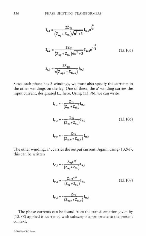
PHASE SHIFTING TRANSFORMERS536
(13.105)
Since each phase has 3 windings, we must also specify the currents inthe other windings on the leg. One of these, the a' winding carries theinput current, designated Iout here. Using (13.96), we can write
(13.106)
The other winding, a", carries the output current. Again, using (13.96),this can be written
(13.107)
The phase currents can be found from the transformation given by(13.88) applied to currents, with subscripts appropriate to the presentcontext,
© 2002 by CRC Press

PHASE SHIFTING TRANSFORMERS 537
and
(13.109)
and
(13.108)
(13.110)
© 2002 by CRC Press

PHASE SHIFTING TRANSFORMERS538
Substituting Ifa,1, Ifa,2, Ifa,0 for the various fault types we obtain, For a3 phase fault:
For a single line to ground fault:
and
(13.111)
(13.112)
© 2002 by CRC Press

PHASE SHIFTING TRANSFORMERS 539
and
For a line to line fault:
and
(13.113)
(13.114)
(13.115)
© 2002 by CRC Press
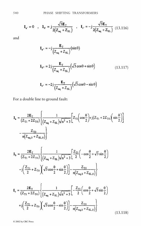
PHASE SHIFTING TRANSFORMERS540
(13.116)
and
For a double line to ground fault:
(13.117)
(13.118)
© 2002 by CRC Press

PHASE SHIFTING TRANSFORMERS 541
and
and
(13.119)
(13.120)
© 2002 by CRC Press

PHASE SHIFTING TRANSFORMERS542
Except for the double line to ground fault, the fault currents can betaken as real in force and stress calculations. In the case of normalcurrents for the units with three windings on a leg, the currents arecomplex. Leakage fields under normal conditions are needed for losscalculations. Thus for double line to ground faults and for leakage fieldcalculations for the standard delta and 2 core design, calculations withcomplex currents must be performed.
© 2002 by CRC Press

543
14. COST MINIMIZATION
Summary Transformer design is primarily determined by minimizingthe overall cost, including the cost of materials, labor, and losses. Thisminimization, however, must take into account constraints which maybe imposed on the transferred power, the impedance, the flux density,the overall height of the tank, etc. Since the cost and constraints aregenerally non-linear functions of the design variables, a non-linearconstrained optimization method is required. We examine several suchmethods, developing in greater detail the one which appears to be bestsuited to our needs. It is then applied to transformer design, consideringfor simplicity only major cost components and constraints.
14.1 INTRODUCTION
A transformer must perform certain functions such as transforming powerfrom one voltage level to another without overheating or withoutdamaging itself when certain abnormal events occur, such as lightningstrikes or short circuits. Moreover, it must have a reasonable lifetime (>20 years) if operated under rated conditions. Satisfying these basicrequirements still leaves a wide latitude in possible designs. A transformermanufacturer will therefore find it in its best economic interest to choose,within the limitations imposed by the constraints, that combination ofdesign parameters which results in the lowest cost unit. To the extentthat the costs and constraints can be expressed analytically in terms ofthe design variables, the mathematical theory of optimization withconstraints can be applied to this problem,
Optimization is a fairly large branch of mathematics with majorspecialized subdivisions such as linear programming, unconstrainedoptimization, and linear or non-linear equality or inequalityconstrained optimization. Transformer design optimization falls intothe most general category of such methods, namely non-linear equalityand inequality constrained optimization. In this area, there are noalgorithms or iteration schemes which guarantee that a global optimum
© 2002 by CRC Press

COST MINIMIZATION544
(in our case a minimum) will be found. Most of the algorithms proposedin the literature will converge to a local optimum with varying degreesof efficiency although even this is not guaranteed if one starts theiterations too far from a local optimum. Some insight is thereforeusually required to find a suitable starting point for the iterations. Oftenpast experience can serve as a guide.
There is however a branch of optimization theory called geometricprogramming which does guarantee convergence to a global minimum,provided the function to be minimized, called the objective or costfunction, and the constraints are expressible in a certain way [Duf67].These restricted functional forms, called posynomials, will be discussedlater. This method is very powerful if the problem functions conform tothis type. Approximating techniques have been developed to cast othertypes of functions into posynomial form. Later versions of thistechnique removed many of its restrictions but at the expense of nolonger guaranteeing that it will converge to a global minimum [Wil67].One of the earliest applications of geometric programming was totransformer design.
Whatever choice of optimization method is made, there is also thequestion of how much detail to include in the problem description.Although the goal is to find the lowest cost, one might wish that thesolution should provide sufficient information so that an actual designcould be produced with little additional work. In general, the moredetail one can generate from the optimization process, the less workwhich will be required later on. However, it would be unrealistic toexpect that the optimum cost design for a transformer, for example,would automatically satisfy all the mechanical, thermal, andelectrical constraints that require sophisticated design codes toevaluate. Rather, these constraints can be included in an approximate(conservative) manner in the optimization process. When the designcodes are subsequently employed, hopefully only minor adjustmentswould need to be made in the design parameters to produce aworkable unit.
We will briefly describe geometric programming, presenting enoughof the formalism to appreciate some of its strengths and weaknesses.Then we will present a more general approach which is developed ingreater detail, since it is applied subsequently to the transformer costminimization problem.
© 2002 by CRC Press

COST MINIMIZATION 545
14.2 GEOMETRIC PROGRAMMING
Geometric programming requires that the function to be minimized, theobjective or cost function, and all the constraints be expressed asposynomials. Using the notation of Ref. [Duf67], these are functions ofthe form
g=u1+u2+···+un (14.1)
with
(14.2)
where the ci are positive constants and the variables t1, t2,…, tm arepositive. The exponents aij can be of either sign or zero. They can alsobe integer or non-integer.
The method makes use of the geometric inequality
(14.3)
where the Ui are non-negative and the δi are positive weights that satisfy
δ1+δ2+···δn=1 (14.4)
called the normality condition. Equality obtains in (14.3) if and only ifall Ui are equal. Letting ui=δiUi, (14.3) can be rewritten
(14.5)
Substituting (14.2) for the ui in (14.5), we obtain
(14.6)
where . If we can choose the weights δi in such a way that
© 2002 by CRC Press

COST MINIMIZATION546
(14.7)
then the right hand side of (14.6) will be independent of the variables tj.(14.7) is called the orthogonality condition. With the Dj's so chosen, theright hand side of (14.6) is referred to as the dual function, v(δ), and isgiven by
(14.8)
where the vector δ=(δ1, δ2,…, δn). Using vector notation for the variablestj, t=(t1, t2,… tn), (14.6) can be rewritten
g(t)≥v(δ) (14.9)
subject to (14.7).As (14.9) shows, the objective function g(t) is bounded below by the
dual function v(δ). Thus the global minimum of g(t) cannot be less thanv(δ) . Similarly the global maximum of v(δ) cannot be greater than g(t).We now show that the minimum of g(t) and the maximum of v(δ) areequal. Let t=t' at the minimum. At this point, the derivative of g(t) withrespect to each variable must vanish,
(14.10)
Since by assumption, (14.10) can be multiplied by tj',
(14.11)
using (14.1) and (14.2). Dividing by g(t') and letting
(14.12)
© 2002 by CRC Press
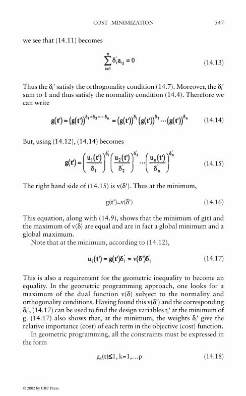
COST MINIMIZATION 547
we see that (14.11) becomes
(14.13)
Thus the δi' satisfy the orthogonality condition (14.7). Moreover, the δi'sum to 1 and thus satisfy the normality condition (14.4). Therefore wecan write
(14.14)
But, using (14.12), (14.14) becomes
(14.15)
The right hand side of (14.15) is v(δ'). Thus at the minimum,
g(t')=v(δ') (14.16)
This equation, along with (14.9), shows that the minimum of g(t) andthe maximum of v(δ) are equal and are in fact a global minimum and aglobal maximum.
Note that at the minimum, according to (14.12),
(14.17)
This is also a requirement for the geometric inequality to become anequality. In the geometric programming approach, one looks for amaximum of the dual function v(δ) subject to the normality andorthogonality conditions. Having found this v(δ') and the correspondingδi', (14.17) can be used to find the design variables tj' at the minimum ofg. (14.17) also shows that, at the minimum, the weights δi' give therelative importance (cost) of each term in the objective (cost) function.
In geometric programming, all the constraints must be expressed inthe form
gk(t)≤≤≤≤≤1, k=1,…p (14.18)
© 2002 by CRC Press

COST MINIMIZATION548
where the gk are posynomials. Write
gk=u1+u2+…un (14.19)
as before with the ui given by (14.2). (We ignore labeling the ui with kfor simplicity.) In dealing with inequality constraints, the weights areallowed to be unnormalized. Letting λ denote their sum, we have
λ=δ1+δ2+…+δn (14.20)
However, in applying the geometric inequality (14.5), we must usenormalized weights given by δi/λ, so we get
(14.21)
Raising everything to the power λ, we obtain
(14.22)
There is an inequality like (14.22) for each constraint. We need to labelthese appropriately to avoid confusion. Let
(14.23)
be a set of integers labeling the terms in constraint k when k>0. We havemo=1, m1=n0+1, m2=n1+1, np=n for a total of n terms in all of the functions.We have m positive variables ti, i=1,…, m. Hence
(14.24)
where go(t)=g(t) is the objective function. We now multiply all of theinequalities together, i.e. the extreme left and right sides of (14.5) and(14.22) for each constraint, to get
© 2002 by CRC Press

COST MINIMIZATION 549
(14.25)
Using (14.24), this becomes
(14.26)
with the auxiliary conditions
(14.27)
which eliminates the tj dependencies. In addition, we have the normalitycondition
(14.28)
All the weights δi are required to be non-negative,
δi≥0, i=l,...n (14.29)
The problem of minimizing the objective function subject to itsconstraints becomes one of maximizing the dual function v(δ) subject tothe dual constraints (14.27), (14.28), and (14.29). These dualconstraints, aside from the non-negativity condition, are linearconstraints in contrast to the, in general, non-linear constraints of theoriginal formulation. There are as many unknowns δi as terms in theobjective plus constraint functions, namely n. However (14.27) and(14.28) must be satisfied by these unknowns and there are m+1 of these,where m is the number of design variables. The degree of difficulty isdefined as n-m-1. When this equals 0, this means that there are as manyunknowns as equations and the solution is found by solving the set oflinear equations (14.27) and (14.28) simultaneously. When this isgreater than 0, techniques for maximizing an, in general, non-linearfunction subject to linear constraints must be employed. Under verygeneral conditions, it can be shown that the minimum of the objectivefunction subject to its constraints equals the maximum of the dual
© 2002 by CRC Press

COST MINIMIZATION550
function subject to the dual constraints [Duf67]. Furthermore at themaximizing point δ', the following equations hold
(14.30)
which permits the determination of the design variables tj' at theminimizing point of the objective function via (14.2).
As a simple example, consider minimizing
subject to
There are four terms in total so that there are four δi. The dual functionis
subject to
This problem has degree of difficulty=0, so the solution is determinedby solving the above linear equations to obtain
The maximum of the dual function is therefore
© 2002 by CRC Press

COST MINIMIZATION 551
The design variables can be found from
These can be solved by taking logarithms or in this case by substitution.The solution is
This solution can be checked by substituting these values into the objectivefunction g(t') which should produce the same value as given by v(δ')above.
When the degree of difficulty is not zero, the method becomes one ofmaximizing a non-linear function subject to linear constraints for whichvarious solution strategies are available. For problems formulated inthe language of geometric programming, these strategies lead to theglobal maximum of the dual function (global minimum of the objectivefunction. This desirable outcome is not, however, without a price. In thecase of transformer design optimization, the number of terms in arealistic cost function, not to mention the constraints, is quite largewhereas the number of design variables can be kept reasonably small.This means that the degree of difficulty is large. In addition, it can bequite awkward to express some of the constraints in posynomial form.A further difficulty is that the constraints must be expressed asinequalities whereas in some cases an equality constraint may bedesired.
© 2002 by CRC Press

COST MINIMIZATION552
14.3 NON-LINEAR CONSTRAINED OPTIMIZATION
The general non-linear optimization problem with constraints can beformulated in the following way:
(14.31)
where f and the ci are non-linear functions in general. We will assumethroughout that they are at least twice differentiate. Although we haveexpressed this optimization in terms of a minimum, maximizing afunction f is equivalent to minimizing -f . Also any equality or inequalityconstraint involving analytic functions can be expressed in the abovemanner. For example, a constraint of the type ci(x)≤0 can be rewritten-ci(x)≥0. Thus the above formulation is quite general.
14.3.1 Characterization of the Minimum
We will be concerned with finding a relative minimum of f(x) subject tothe constraints. This may or may not be a global minimum for the particularproblem considered. We first consider how to characterize such aminimum, i.e. how do we know we have reached a relative minimumwhile satisfying all the constraints. Let x* denote the design variablevector at a minimum. In this section, minimum always means relativeminimum. If an inequality constraint is not active at the minimum, i.e.ci(x*)>0, then it will remain positive in some neighborhood about theminimum, (An inequality constraint is active if ci(x)=0 and it is said to beviolated if ci(x)<0.) Thus one could move some small distance away fromthe minimum without violating this constraint. In effect, near the minimum,this constraint places no restrictions on the design variables. It can thereforebe ignored. Only those inequality constraints which are active play a rolein characterizing the minimum. We therefore include them in the list ofequality constraints in our formulation (14.31). Strategies to add or dropinequalities from the list of equality constraints will be discussed later.
Much of the methodology presented in this section is based on Ref.[Gil81]. We adopt their notation which is briefly reviewed here. First a
© 2002 by CRC Press

COST MINIMIZATION 553
distinction is made between column and row vectors. A column vectoris denoted by
where the vi are its components. If there are n components, it can also bereferred to as an n-vector. Its transpose is a row vector, i.e.
vT=(v1 v2 ··· vn)
where T denotes transpose. The dot or scalar product between two vectorsv and w is given by
vTw=v1w1+v2w2+···+vnwn
It is essentially the matrix product between a row and column vector inthat order. If the order were reversed, we would have
i.e. the matrix product between a column and row vector in that order.A matrix M is called an m×n matrix if it has m rows and n columns.The i, j th matrix element is denoted Mij and these are organized into anarray
A matrix vector product between an m×n matrix and an n-vector, denotedMv, is an m-vector whose components are
© 2002 by CRC Press

COST MINIMIZATION554
If we multiply on the left by a row m-vector wT, we get the scalarproduct between w and the above vector
Further notation will be introduced as it is encountered.Using Taylor’s theorem, expand the functions f(x) and the ci(x) about
the minimizing point x*. Let x=x*+εp, where p is an n-dimensionalvector and ε a positive constant. Then
(14.32)
where g is the gradient vector and is given by
(14.33)
G is the Hessian matrix which is given by
(14.34)
The Hessian matrix is symmetric because of the equality of mixed partialderivatives. Vector dot products or matrix products are implied in (14.32).Higher order terms in the expansion (14.32) are assumed to be small forthe values of ε considered.
Similarly we have for the equality constraints
© 2002 by CRC Press

COST MINIMIZATION 555
(14.35)
where ai is its gradient vector and Gi its Hessian matrix. Here ci(x*)=0.We would like to continue to satisfy the constraints as we move awayfrom the minimum since they are assumed to apply for any choice ofdesign parameters. This means that the first order term, i.e. the term inε should vanish,
(14.36)
There is an equation like this for each equality constraint. Let A denotea matrix whose i-th row is . Then (14.36) can be expressed compactlyfor all equality constraints as
Ap=0 (14.37)
A has t rows and n columns. It also depends on x or x* but we omit thisfor clarity. We assume that t≤n and that A has full row rank, i.e. that theconstraint gradient vectors ai are linearly independent. If this is not true,then one or more of the constraints is redundant (to first order) and canbe dropped from the list.
From (14.37), we see that p must be orthogonal to the row space ofA. Thus p lies in the orthogonal complement of this row space. (Anyvector space is decomposable into disjoint subspaces which areorthogonal complements of each other.) Let Z denote a matrix whosecolumn vectors form a basis of this orthogonal subspace of dimensionn-t. Thus Z has n rows and n-t columns. This orthogonality can beexpressed by
AZ=0 (14.38)
Since p lies in this orthogonal subspace, it can be expressed as a linearcombination of its basis vectors, that is a linear combination of thecolumn vectors of Z. Thus
p=Zpz (14.39)
where pz is a vector of dimension n-t.
© 2002 by CRC Press

COST MINIMIZATION556
Probably the best way to obtain Z is via a triangularization of Ausing Hausholder transformation matrices. These are orthogonalmatrices of the form
(14.40)
where w is a vector of magnitude |w| and I is the unit diagonal matrix.By suitably choosing w, the columns of any matrix can be successivelyput in upper triangular form [Gol89]. In our case, we apply this procedureto AT to obtain
(14.41)
where Q is an n×n orthogonal matrix since it is the product oforthogonal matrices, R is an upper triangular matrix of dimension t×t,and 0 is a zero matrix of dimension (n-t)×t. Taking the transpose of(14.41), we get
AQT=(L 0) (14.42)
where L=RT is a lower triangular matrix and 0 is the t×(n-t) zero matrix.Thus we can take Z to be the last n-t columns of QT since these areorthogonal to the rows of A. Since Q is an orthogonal matrix, its columnvectors form an orthonormal basis for the whole space. Thus the first tcolumns form an orthonormal basis for the row space of A and the lastn-t columns form an orthonormal basis for its orthogonal complement.We group the first t columns into a matrix called Y so that
QT=(Y Z) (14.43)
With p restricted to the form (14.39), the expression (14.32) becomesto first order
f(x*+εp)=f(x*)+εgT(x*)Zpz+··· (14.44)
For f(x*) to be a minimum, we must have
© 2002 by CRC Press

COST MINIMIZATION 557
f(x*+εp)≥f(x*) (14.45)
In order for this to hold, the term in ε in (14.44) must be positive or zero.Since ε is positive, if this term is non-zero for some vector pz, it can bemade negative by possibly changing pz to -pz and thus violate (14.45).Hence we must require at the minimum
gT(x*)Z=0 (14.46)
This implies that the gradient is in the row space of A. Therefore
g(x*)=ATλ* (14.47)
where λ* is a vector of dimension t called the vector of Lagrangemultipliers. (Note that the column space of AT is the row space of A.
Let us now consider that one of our equality constraints at theminimum was originally an inequality constraint. Let this be the cj thconstraint. Then a displacement vector p could be chosen so that
Cj(x*+εp)≥0 (14.48)
without violating the constraint. Noting that cj(x*)=0, from (14.35) withj replacing i, we see that to first order in ε, we get
(14.49)
Assume that p satisfies the other constraints, i.e. (14.36) holds for i≠j.Then rewriting (14.47), we have
(14.50)
where we have omitted the dependence of the a's on x*. For the abovechoice of p,
(14.51)
© 2002 by CRC Press
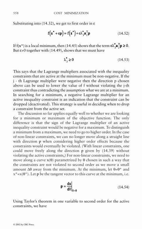
COST MINIMIZATION558
Substituting into (14.32), we get to first order in ε
(14.52)
If f(x*) is a local minimum, then (14.45) shows that the term .But ε>0 together with (14.49), shows that we must have
(14.53)
This says that the Lagrange multipliers associated with the inequalityconstraints that are active at the minimum must be non-negative. If thej - th Lagrange multiplier were negative then the direction p chosenabove can be used to lower the value of f without violating the j-thconstraint thus contradicting the assumption what we are at a minimum.In searching for a minimum, a negative Lagrange multiplier for anactive inequality constraint is an indication that the constraint can bedropped (deactivated). This strategy is useful in deciding when to dropa constraint from the active set.
The discussion so far applies equally well to whether we are lookingfor a minimum or maximum of the objective function. The onlydifference is that the sign of the Lagrange multiplier of an activeinequality constraint would be negative for a maximum. To distinguisha minimum from a maximum, we need to go to higher order. In the caseof non-linear constraints, we can no longer move along a straight linewith direction p when considering higher order effects because theconstraints would eventually be violated. (With linear constraints, onecould move freely along the direction p given by (14.39) withoutviolating the active constraints,) For non-linear constraints, we need tomove along a curve x(θ) parametrized by θ chosen in such a way thatthe constraints are not violated to second order as we move a smallamount ∆θ away from the minimum. At the minimum, let θ=θ* andx*=x(θ*). Let p be the tangent vector to this curve at the minimum, i.e.
(14.54)
Using Taylor’s theorem in one variable to second order for the activeconstraints, we have
© 2002 by CRC Press

COST MINIMIZATION 559
(14.55)
All derivatives are evaluated at θ*. Using the chain rule, we obtain
(14.56)
and, using (14.56),
where Gi is the Hessian of the i-th constraint defined previously. Sinceci(x*)=0 at the minimum, in order for (14.55) to vanish to second order,we must have both (14.56) and (14.57) vanish. The vanishing of (14.56)yields the first order results such as (14.36) previously derived. Thevanishing of (14.57) yields the new second order results. Just as wepreviously turned (14.56) into a matrix equation so it applied to all theconstraints, equation (14.37), we apply the same procedure to (14.57),Organizing the into rows of the A matrix and setting (14.57) to zero,we get
(14.58)
Now consider the behavior of the objective function f along thiscurve which satisfies the constraints to second order. Using Taylor’stheorem again in one variable,
14.57
© 2002 by CRC Press
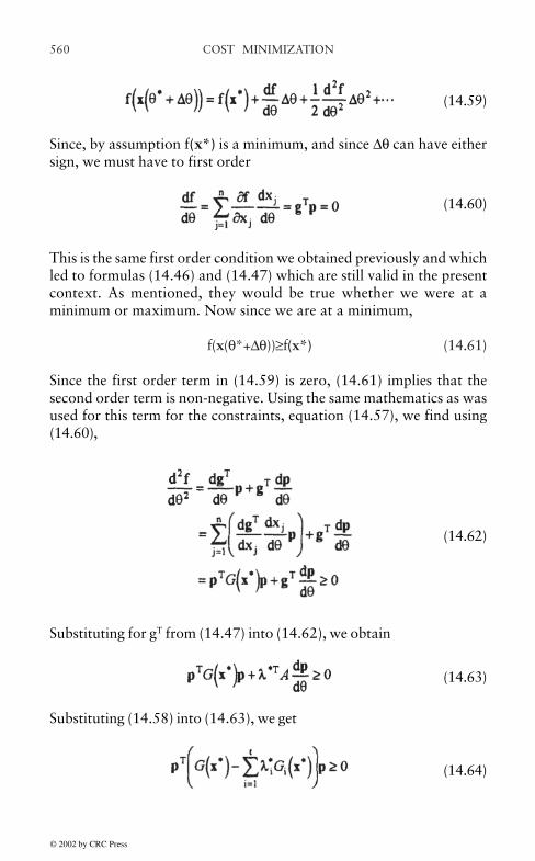
COST MINIMIZATION560
(14.59)
Since, by assumption f(x*) is a minimum, and since ∆θ can have eithersign, we must have to first order
(14.60)
This is the same first order condition we obtained previously and whichled to formulas (14.46) and (14.47) which are still valid in the presentcontext. As mentioned, they would be true whether we were at aminimum or maximum. Now since we are at a minimum,
f(x(θ*+∆θ))≥f(x*) (14.61)
Since the first order term in (14.59) is zero, (14.61) implies that thesecond order term is non-negative. Using the same mathematics as wasused for this term for the constraints, equation (14.57), we find using(14.60),
(14.62)
Substituting for gT from (14.47) into (14.62), we obtain
(14.63)
Substituting (14.58) into (14.63), we get
(14.64)
© 2002 by CRC Press

COST MINIMIZATION 561
Using (14.39) for p, (14.64) becomes
(14.65)
Since (14.65) must be true for any choice of pz, this requires thematrix within the square brackets to be positive semi-definite. Oftenminimization with constraints is formulated in terms of a Lagrangianfunction
(14.66)
Then (14.47) follows from requiring the Lagrangian to vanish to firstorder at the minimum and (14.65) follows from requiring the projectedHessian of the Lagrangian to be positive semi-definite. (The Hessian isprojected by means of the Z matrix,) The Lagrangian approach doesnot appear to be as well motivated as the one we have taken.
Condition (14.65) together with (14.47) are necessary conditions fora minimum subject to the constraints. They are not, however, sufficient.This is because if (14.65) were 0 for some non-zero vector pz, the pointx* could be a saddle point. To eliminate this possibility, the inequalityin (14.65) must be replaced by a strict inequality, >, so that the matrix ispositive definite. This is sufficient to guarantee a minimum. We willassume this requirement to be met in the minimization problems wedeal with.
14.3.2 Solution Search Strategy
Because the functions we are dealing with are, in general, non-linear,iterations are required in order to arrive at a minimum from some startingset of the design variables. Assuming the iterations converge, we canthen check that the conditions derived in the previous section hold at theconverged point to guarantee that it is a minimum. This may or maynot be a global minimum. However, if suitable starting values are chosenbased on experience, then for most practical problems, the minimumreached will be, with high probability, a global minimum.
One of the best convergence strategies is Newton-Raphson iteration.Provided one is near the minimum, this method converges very rapidly.
© 2002 by CRC Press

COST MINIMIZATION562
In fact, for a quadratic function, it converges in one step. Applying thismethod to the constraint functions, with p=∆x, we get
(14.67)
Collecting these into a vector of constraint functions, c(x)=(c1 c2… ct)and using the matrix A whose rows are ai
T as defined previously, (14.67)can be written to include all the active constraints as
A(x)p=-c(x) (14.68)
where the dependence of A on the value of x at the current iterate isindicated. Since p is an n-vector in the space of design variables, we canexpress it in terms of the basis we obtained from the QR factorization ofA. Thus, using (14.43)
p=YpY+ZpZ (14.69)
where pY is a t-vector in the row space of A and pZ is an (n-1)-vector inits orthogonal complement. Using (14.38), (14.68) becomes
AYpY=-c(x) (14.70)
where the dependence of the matrices on x has been supressed for clarity.However, from (14.42) and (14.43), we see that AY=L. Thus (14.70)becomes
LpY=-c(x) (14.71)
Since L is a lower triangular matrix, (14.71) can be solved readilyusing forward substitution. Thus the QR factorization of A has anadditional benefit in facilitating the solution of a matrix equation.
We now apply the Newton-Raphson technique to (14.47) which mustbe satisfied at the minimum
(14.72)
© 2002 by CRC Press
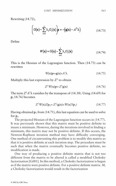
COST MINIMIZATION 563
Rewriting (14.72),
(14.73)
Define
(14.74)
This is the Hessian of the Lagrangian function. Then (14.73) can berewritten
W(x)p=-g(x)+ATλ (14.75)
Multiply this last expression by ZT to obtain
ZTW(x)p=-ZTg(x) (14.76)
The term ZTATλ vanishes by the transpose of (14.38). Using (14.69) forp, 14.76) becomes
ZTW(x)ZpZ=-ZT(g(x)+W(x)YpY) (14.77)
Having obtained pY from (14.71), this last equation can be used to solvefor pz.
The projected Hessian of the Lagrangian function occurs in (14.77).It was previously shown that this matrix must be positive definite toinsure a minimum. However, during the iterations involved in finding aminimum, this matrix may not be positive definite. If this occurs, theNewton-Raphson iteration method may have difficulty converging.One method of circumventing this problem is to modify this matrix sothat it is positive definite at each iteration step. The procedure must besuch that when the matrix eventually becomes positive definite, nomodification is made.
One way of producing a positive definite matrix that is not toodifferent from the matrix to be altered is called a modified Choleskyfactorization [Gil81]. In this method, a Cholesky factorization is begunas if the matrix were positive definite. For a positive definite matrix. M,a Cholesky factorization would result in the factorization
© 2002 by CRC Press

COST MINIMIZATION564
M=PDPT (14.78)
where P is a lower triangular matrix and D a positive diagonal matrix,i.e. a diagonal matrix with all positive elements. If, during the course ofthe factorization of a not necessarily positive definite matrix, an elementof D is calculated to be zero or negative, the corresponding diagonalelement of M is increased until the element of D becomes positive.Limitations are also placed on how large the values of P can becomeduring the factorization. These limitations can also be achieved byincreasing the diagonal values of the original matrix. The result is aCholesky factorization of a modified matrix M2 which is related to theoriginal matrix by
M'=PDPT=M+E (14.79)
where E is a positive diagonal matrix. Using this approach, (14.77) issolved for pz at each iteration.
With pY and pZ determined, the complete step given by (14.69) isknown. This step may, however, be too large. Some of the equalityconstraints may be violated to too great an extent or the objectivefunction may not decrease. The step may also be so large as to violatean inequality constraint that is not active. We would like to keep thedirection of p but restrict its magnitude based on these considerations.Consider multiplying p by ε to get a step εp. By letting ε vary from 0 to1, we can check these other criteria at each ε, stopping when theybecome too invalidated or when ε=1. One of these criteria would be thatwe not violate any of the inactive inequality constraints. If this occurs atsome value of ε≤1, then this restricts the step size and the constraintwhich is just violated is added to the list of active constraints on the nextiteration. Another criteria to use to restrict the step size is to define amerit function which measures to what extent the constraints aresatisfied and to what extent the objective function is decreasing in valuealong the step. One choice for this function is
(14.80)
where ρ is a positive constant. The values of ε are increased towards 1so long as this merit function decreases or until one of the inactiveconstraints is violated. When this function starts increasing or an inactive
© 2002 by CRC Press

COST MINIMIZATION 565
constraint is violated, that value of ε is used to determine the step sizeεp. In this approach, units must be chosen so that the relative magnitudesof f and the ci are close. This means that, for values of x which can beexpected to violate the constraints during the iterations, the values of fand the ci are of the same order of magnitude. Then ρ can really be usedto weigh the importance of satisfying the constraints relative to achievinga minimum of the objective function. In our work, we have chosenρ=20. Thus we gradually increase ε until either the merit function startsincreasing or an inactive constraint is violated or ε=l, whichever comesfirst.
Having chosen ε, we solve for new values of the Lagrangemultipliers using (14.75) with p replaced by the actual step taken, εp.Rearranging (14.75), we obtain
ATλ=g(x)+W(x)εp (14.81)
which is an equation for the unknown λ, since all other quantities areknown. The solution of this equation is also facilitated by the results ofthe QR factorization of A. From (14.41), we can write
(14.82)
since QTQ=QQT=I for orthogonal matrices. Here I is the unit diagonalmatrix. Substituting into (14.81) and multiplying by Q, we obtain
(14.83)
But, using (14.43), this becomes
(14.84)
Only the top t equations in (14.84) are needed to determine λ and theseare
© 2002 by CRC Press

COST MINIMIZATION566
Rλ=YT(g(x)+W(x)εp) (14.85)
Since R=LT is upper triangular, (14.85) can be directly solved by backsubstitution. This value of λ is used in the next iterate. At the start, allthe λi are set to 1.
At the next iterate, the values of the design variables become
xnew=xold+εp (14.86)
where old labels the present values and new the new values for the designvariables. This process is continued until successive iterations producenegligible changes in the design variables and the Lagrange multipliers.At this point, it is necessary to check that the conditions which shouldhold at a minimum are satisfied. Thus the projected Hessian of theLagrangian should be positive definite and the gradient of the objectivefunction should satisfy (14.47) to some level of accuracy. The equalityconstraints should also equal 0 to some level of accuracy. The Lagrangemultipliers of the inequality constraints which are active at the minimumshould be positive. None of the inequality constraints should be violated,i.e. <0.
During the course of the iterations, the number of equalityconstraints may change as inequality constraints are added or droppedfrom the list of active constraints. They are added when a step sizethreatens to violate an inactive constraint and they are dropped when aLagrange multiplier becomes negative. Strictly speaking, the Lagrangemultiplier of an active inequality constraint only needs to be positive atthe minimum. This does not have to hold away from the minimum asoccurs during the iterations. However, there will be some neighborhoodabout the minimum where they will remain positive if the constraint isactive at the minimum. We also noted previously that the gradients ofthe active constraints are assumed to be linearly independent. If this isnot true, then constraints are dropped until a linearly independent set isobtained. This is determined during the QR factorization of A since theprocess requires the rows of A to be linearly independent.
For certain types of problems, it may be necessary for all or some ofthe variables to be positive. This can be treated as a special type ofinequality constraint. Thus if variable xj must be positive, we add to thelist of constraints
ck(x)=xj≥0 (14.87)
© 2002 by CRC Press

COST MINIMIZATION 567
where k labels the inequality constraint. The gradient vector for thisconstraint is given by
(14.88)
where the 1 is in the j-th position. Its Hessian matrix is identically zero.Thus, this type of restriction can be handled like an ordinary inequalityconstraint. It has no influence on the minimization unless xj becomes 0or negative during the course of the iterations,
14.3.3 Practical Considerations
It is useful to choose units so that all the design variables are comparablein magnitude. It is also desirable to keep the objective function and theconstraints (violated to some degree or away from 0 if inequalities) ofcomparable magnitude. A good choice for this magnitude is unity. Forexample, if the objective function is cost, one could express it in $,kilo$, or mega$, whichever produces a value of order of magnitudeunity at the minimum. Similarly an equality or inequality constraint ofthe form
A+B+C+D+···≥0
could be divided by the absolute value of the maximum term so as tobring it closer to 1. This may not be possible in all cases so some otherstrategy may be necessary. This procedure will prevent the merit functionfrom favoring one constraint more that another.
Although the method developed here applies to any non-linear, twicedifferentiate objective or constraint functions, in practice it is found thatthese functions are often of the form
(14.89)
where the coefficients b, and the exponents aij are arbitrary constants.This differs from the posynomials considered earlier where the coefficientsbi all had to be positive. The k-th component of the gradient vector ofthis function is given by
© 2002 by CRC Press

COST MINIMIZATION568
(14.90)
The k, q-th entry of its Hessian matrix, where k≠q, is given by
(14.91)
When k=q, the diagonal entry of the Hessian matrix is
(14.92)
Some care must be exercised in using the above formulas when a variableor an exponent vanishes. Also when a variable is negative and thecorresponding exponent in non-integer, the expression becomesimaginary. In the latter case, which could occur during the iterationseven if the variables are constrained to be non-negative, the exponent issimply rounded off to the nearest integer. This allows the iterations toproceed. Eventually as the minimum is approached, the appropriatevariables will become non-negative so that this rounding becomesunnecessary. If a variable is expected to be negative at the minimum,then it should occur with an integer exponent in all the functions,
14.4 APPLICATION TO TRANSFORMER DESIGN
In designing a transformer, we normally wish to minimize the cost. Ourobjective function f(x) is therefore a cost function. It will, in general,have many terms. These will include material costs, labor costs, thecost of losses to the customer, and overhead costs. These componentcosts, as well as the constraint functions, must be expressed in terms ofa basic set of design variables. Although the choice of design variablesis somewhat arbitrary, they should be chosen in such a way that the costand constraint functions can be easily expressed in terms of them. Herewe consider a 2 winding, 3 phase, core-form power transformer. Wewill simplify the details in order to focus more on the method.
© 2002 by CRC Press

COST MINIMIZATION 569
14.4.1 Design Variables
Our basic design variables are:
(1) B Core flux density in Tesla(2) Js OA current density in the secondary or LV winding in kAmps/in2
(3)Re Core radius in inches(4)g HV-LV gap in inches(5)Rs Mean radius of the secondary or LV winding in inches(6)Rp Mean radius of the primary or HV winding in inches(7)hs Height of the secondary winding in inches(8)ts Thickness (radial build) of the secondary winding in inches(9)tp Thickness (radial build) of the primary winding in inches(10)Mc Weight of the core steel in kilo-pounds(11)Mt Weight of the tank in kilo-pounds
Note that the last two weights can be expressed in terms of the otherdesign variables. However, since some of the material and labor costsand losses are easily expressed in terms of them, we find it convenient toinclude them in the set of basic design variables. Their dependence onthe other variables will be expressed in terms of equality constraints.The units chosen for the above variables are such that their magnitudesare all in the range of about 1 to 100. These units are used internally inthe computer optimization program. As far as input and output isconcerned, i.e. what the user deals with, the units are a matter offamiliarity and can differ from the above.
Figure 14.1 illustrates some of the design variables geometrically.We have not considered the height of the primary winding a designvariable since, in our designs, it is usually taken to be an inch shorterthen the secondary winding. We express this as hp=αhs, where hp is theheight of the primary winding and α is a fraction ≈0.95. gc and go aregaps which are fixed and inputted by the user, gc depends on whether atertiary or tap winding is present under the LV winding and go dependson the phase to phase voltages. H is the window height and T thewindow width. X is the maximum stack width ≈2Rc. These areexpressible in terms of the other variables.
© 2002 by CRC Press

COST MINIMIZATION570
14.4.2 Cost Function
One of the cost components is the cost of the copper. To obtain this, weneed the copper weight. In terms of the design variables, the weight ofthe 3 secondary windings (for 3 phases) is
Ms=3dCu ηs(2πRshsts) (14.93)
where dCu is the copper density and ηs is the fill factor, i.e. the fraction ofthe coil’s cross-sectional area which is copper. If this is in pounds, itmust then be multiplied by a $/lb cost to arrive at the cost to include inthe objective function. This $/lb cost must reflect the cost of the rawcopper plus the add-on cost of forming it into an insulated wire or cable
Figure 14.1 Geometry of a 2 winding core-form power transformer illustratingsome of the design variables
© 2002 by CRC Press

COST MINIMIZATION 571
plus any overhead or storage costs. The fill factor will be determinedseparately by selecting a cable size which meets constraints on the coil’scross sectional dimensions and the number of turns. If a tertiary or tapwinding is present, its cost is determined as some fraction of the secondarywinding’s cost. The weight of the primary winding is similarly
Mp=3dCu ηpα(2πRphstp) (14.94)
where ηp is the primary winding’s fill factor. This also gets multipliedby a $/lb which will differ from that of the secondary winding becauseit will generally be made of a different type of wire or cable.
The weight of the core in pounds is simply 1000Mc. This ismultiplied by a $/lb for the core steel before inclusion in the costfunction. This $/lb also includes overhead and storage costs. The tankcost is similarly 1000Mt times the appropriate $/lb. Mc and Mt will beexpressed in terms of the other variables by means of equalityconstraints.
Other material costs are the cost of the oil, the insulation such ascylinders, key-spacers, and lead support structure, the cost of leads,clamping, bushings, tap-gear, conservator if present, radiators, andauxiliary reactors or series transformers. The details are omitted here tosimplify the discussion.
Load and no-load losses are part of the overall cost of operating atransformer and are included in the cost function. A customer buys atransformer not on just its initial manufacturing cost but also on thecost of operating it over many years. These latter costs depend on howefficient the unit is, i.e. how high are its losses. The load losses includethe Joule heating in the windings (copper losses) and the losses due tothe stray flux impinging on tank walls, clamps, etc. (stray losses). Thelosses in the secondary winding under OA conditions can be expressedas
(14.95)
where ρCu is the copper resistivity which is evaluated at the appropriatetemperature, ecfs is the eddy current factor which is due to stray fluxand depends on the type of wire or cable making up the winding. Vs isthe copper volume which can be expressed
Vs=3ηs(2πRshsts) (14.96)
© 2002 by CRC Press

COST MINIMIZATION572
Since Js is in kA/in2, ρs needs to be in appropriate units and an overallmultiplying factor is necessary to get Ws in kW. This must then bemultiplied by the cost of load losses in $/kW. Similarly, the primarywinding’s losses are given by
(14.97)
where the copper volume is
Vp=3ηpα(2πRphstp) (14.98)
and where Jp is the current density in the primary winding under OAconditions. Because the ampere-turns of the primary and secondary areequal under balanced conditions, we can obtain Jp in terms of Js by
(14.99)
This is then substituted into (14.97). We then multiply Wp by the $/kWcost of load losses before adding it to the cost function. The stray lossesare also part of the load losses and must be added to the cost functionbut we omit discussing them here for simplicity. If the transformerincludes a reactor, step voltage regulator, or series transformer, then thecost of losses associated with these components must be added to thecost function,
The no-load losses are essentially the core losses. Generally the coresteel manufacturer provides a curve or polynomial expression for thecore losses in W/1b in terms of the core flux density, e.g.
Multiplying this by the core weight in pounds, 1000Mc, gives a coreloss for an ideal core. Actual cores have higher losses due to non-uniformflux in the comers, due to building stresses, and other factors. Thesemust be accounted for in the expression for the no-load loss. Havingdone this, the core loss in kW is then multiplied by the cost of the noloadlosses in $/kW before adding to the cost function,
Labor costs are an important part of the cost of a transformer sincepower transformers are usually custom made. The various specialized
© 2002 by CRC Press
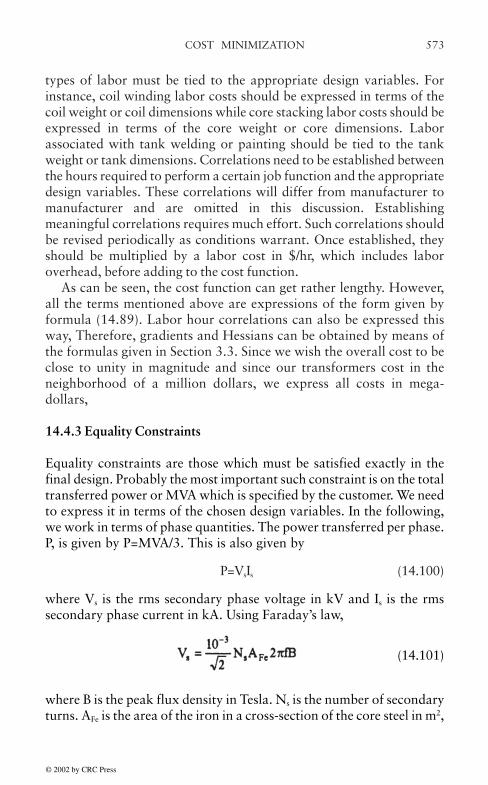
COST MINIMIZATION 573
types of labor must be tied to the appropriate design variables. Forinstance, coil winding labor costs should be expressed in terms of thecoil weight or coil dimensions while core stacking labor costs should beexpressed in terms of the core weight or core dimensions. Laborassociated with tank welding or painting should be tied to the tankweight or tank dimensions. Correlations need to be established betweenthe hours required to perform a certain job function and the appropriatedesign variables. These correlations will differ from manufacturer tomanufacturer and are omitted in this discussion. Establishingmeaningful correlations requires much effort. Such correlations shouldbe revised periodically as conditions warrant. Once established, theyshould be multiplied by a labor cost in $/hr, which includes laboroverhead, before adding to the cost function.
As can be seen, the cost function can get rather lengthy. However,all the terms mentioned above are expressions of the form given byformula (14.89). Labor hour correlations can also be expressed thisway, Therefore, gradients and Hessians can be obtained by means ofthe formulas given in Section 3.3. Since we wish the overall cost to beclose to unity in magnitude and since our transformers cost in theneighborhood of a million dollars, we express all costs in mega-dollars,
14.4.3 Equality Constraints
Equality constraints are those which must be satisfied exactly in thefinal design. Probably the most important such constraint is on the totaltransferred power or MVA which is specified by the customer. We needto express it in terms of the chosen design variables. In the following,we work in terms of phase quantities. The power transferred per phase.P, is given by P=MVA/3. This is also given by
P=VsIs (14.100)
where Vs is the rms secondary phase voltage in kV and Is is the rmssecondary phase current in kA. Using Faraday’s law,
(14.101)
where B is the peak flux density in Tesla. Ns is the number of secondaryturns. AFe is the area of the iron in a cross-section of the core steel in m2,
© 2002 by CRC Press

COST MINIMIZATION574
and f is the frequency in Hz. Expressing AFe in terms of our designvariables, we have
(14,102)
where 0.0254 converts inches to meters and ηc is a fill factor for the coresteel, i.e. the fraction of actual steel in a circle of radius Rc. The currentIs is given in terms of the current density by
(14.103)
Substituting these into the expression for power, we see that Ns cancelsout and we find
(14,104)
Divide by P to get this to be or order 1 and express it in the form of ourstandard equality constraints, ci(x)=0,
(14.105)
This is an expression of the form (14.89). Note that “1 is of this formwith all the aij=0, b1=”1, and m=1. We have kept the numerical constantsexplicit in (14.105) in order to reduce errors,
Perhaps the next most important equality constraint is on the per unitreactance between the primary and secondary windings which isspecified by the customer. A simplified expression for this which workswell in practice is
(14.106)
where r is the co-ratio (=1 for a two winding transformer). Rg is themean radius of the gap between the primary and secondary windingsand is given by
© 2002 by CRC Press

COST MINIMIZATION 575
(14.107)
h is the average height of the two windings,
(14.108)
s is a correction factor for fringing flux,
(14.109)
(VI)b is the base MVA/phase=P and (V/N)b is the base kV/turn which isobtained from (14.101),
(14.110)
Substituting into (14.106) and converting to standard form, we obtain
This is in the form of equation (14.89) and has been suitably normalizedto order of magnitude 1. The constants are again kept explicit to reduceerrors.
We treated Rp as an independent variable thus far since it appears inmany formulas. However, it can really be expressed in terms of otherdesign variables as
(14.112)
(14.111)
© 2002 by CRC Press

COST MINIMIZATION576
Converting to standard form and suitably normalizing, we get the equalityconstraint
(14.113)
An equality constraint is needed for the core weight in kilo-lbs. In termsof the window height H, window width T, and the maximum sheetwidth X which make up the core stacks shown in Fig. 14.1, this is givenby
(14,114)
The last term is a correction factor for the joints. dFe is the density ofthe core iron in lbs/in3. In terms of the basic design variables,
H=hs+slacks (14.115)
where slack, is a slack distance in the window which depends on thevoltage or BIL of the winding and is a constant for the unit underconsideration,
(14.116)
and X will be taken here as 2Rc although a more exact formula can beused for greater accuracy. Thus we obtain, in standard normalized form,
(14.117)
There is an equality expressing the tank weight in terms of the othervariables. The tank dimensions depend, not only on the size of the 3phase core and coils but also on clearances based on voltageconsiderations and on the presence of reactors, tap leads, etc. Theexpression is fairly complicated and is omitted here.
© 2002 by CRC Press

COST MINIMIZATION 577
14.4.4 Inequality Constraints
We place an inequality constraint on the mean radius of the LV windingsince it must not drop below a minimum value given by
(14.118)
Expressing this in standard form, we have
(14.119)
The HV-LV gap g must not fall below a minimum value given byvoltage or BIL considerations. Calling this minimum gap gmin, leads tothe inequality
g≥gmin (14.120)
or, in standard form
(14.121)
The flux density B is limited above by the saturation of iron or by alower value determined by overvoltage or sound level considerations.Calling the maximum value Bmax leads to the inequality in standardform
(14.122)
There is also a reasonable limit on the OA current density. Js, which wecall Jmax. This is based on cooling considerations which are most severeunder FA conditions. But since the FA current density is related to theOA current density by the ratio of FA and OA MVA's, the currentlimitation can be placed on the OA current density. Thus we have, instandard form
(14.123)
© 2002 by CRC Press

COST MINIMIZATION578
It may be necessary to limit the tank height for shipping purposes,Referring to Fig. 14.1, the tank height can be expressed as
H+2X+slackt≤Hmax (14.124)
where Hmax is the maximum tank height and slackt is the vertical slackof the core in the tank and will depend on the clamping structure, thepresence of leads, etc, slackt will be a constant for a given unit. H isgiven by (14.115) and, taking X≈2Rc, we get
hs+4Rc+slacks+slackt ≤Hmax (14.125)
or, in standard form,
(14.126)
The quantity in parentheses in the above formula is a constant for theunit under consideration.
There are other inequalities involving the radial forces on thewindings which are limited by the tensile strength of the copper used,the cooling capacity of the windings which depends on the windingcurrent density and fill factor, and the impulse strength which dependson the cable type, voltage level, etc. These inequalities are fairlyinexact since detailed design codes are ultimately used to determinewinding stresses, temperatures, and impulse voltages. Nevertheless,they place some restrictions on the initial design so that later on, in thedetailed design phase, difficulties are not encountered. In addition, allthe design variables are positive so that a positivity condition on thesevariables must be included among the inequality constraints.
14.4.5 Optimization Strategy
A transformer cost minimization program has been developed based onthe formulation described above. It uses the 11 basic design variablesdiscussed earlier. Initial values must be selected for these variables tostart the iteration process. Because of the equality constraints, of whichthere are 5, we can only select 6 variables independently. For these, wechoose an initial value for B, Binit=0.9Bmax, where Bmax is the maximumflux density specified in the input, an initial value for Js, Js,init=0.75Jmax,
© 2002 by CRC Press

COST MINIMIZATION 579
where Jmax is the inputted maximum OA current density, an initial valuefor g, ginit=gmin, with gmin the inputted minimum high-low gap, an initialvalue for hs, hs,init=60, i.e. a secondary coil height of 60 inches is typicalfor many of our units, an initial value for ts, ts,init=3, i.e. a secondary coilwidth of 3 inches, and an initial value for tp, tp,init=4, i.e. a primary coilwidth of 4 inches, both coil widths typical for our units. We also choose,for starting values, ηs=ηp=0.5, ηc=0.88, and ecfs=ecfp=0.1. The remainderof the starting values for the design variables are determined by satisfyingthe equality constraints or equations such as Faraday’s law which wasused in their derivation or by other means based on convenience. Forgreater flexibility, the user can override the starting values for the 6variables mentioned above.
The iterations are then started. The cost and constraint functions areevaluated, together with their gradients and Hessians. The Lagrangemultipliers are initially set to 1 for the equality constraints. TheHessian of the Lagrangian is then formed. The matrix A is formed andsubjected to a QR factorization. During this process, if a row vector ofA is found to be linearly dependent on the other row vectors, thecorresponding constraint is dropped from the active set. This processproduces the Y, Z, L, and R=LT matrices. The vector pY is then obtainedvia equation (14.71). Equation (14.77) is then solved for pz using amodified Cholesky factorization method. The new step direction is thendetermined, p=YpY+Zpz . The merit function (14.80) is then evaluated forsteps of size εp where ε increases from 0 to 1 in small increments. Thisprocess continues until (1) the merit function starts increasing, (2) one ofthe inequality constraints is violated, or (3) ε=1. If (2) is true, then theviolated constraint is included among the active constraints on the nextiteration. For the value of ε determined by the above procedure, newLagrange multipliers are determined by means of (14.85). If one ofthese is negative for an active inequality constraint, that constraint isdropped from the active set on the next iteration. A new set of designvariables in then determined, using (14.86), and the process repeateduntil convergence is achieved, i.e. until the changes in the designvariables and Lagrange multipliers are negligible. At convergence, theprojected Hessian of the Lagrangian must be positive definite, theequality constraints must be satisfied to a given level of accuracy, theinequality constraints must not be violated, and (14.47) must besatisfied to a given level of accuracy.
At this stage, details concerning the wire or cable types for the twowindings are worked out based on the optimum dimensions hs, ts, hp=αhs, and tp. From the formula for the given power per phase. P,
© 2002 by CRC Press

COST MINIMIZATION580
P=VsIs=VpIp (14.127)
where Vs and Vp are known (inputted) secondary and primary voltages,we can determine the phase currents Is and Ip for the secondary andprimary windings respectively. From these phase currents and theoptimized current densities Js and Jp, we obtain secondary and primaryturn areas As=Is/Js and Ap=Ip/Jp. We use (14.110) to get Volts/turn interms of the optimized variables and, using the known secondary andprimary voltages, we obtain the number of secondary and primary turnsNt and Np. In addition, from the BIL levels of the windings which areinputted, we obtain, via tables, the required paper and key spacerthicknesses for the two windings. Staying within these constraints, awire size (magnet wire or cable) is selected by a search procedure fromthose that are available. In arriving at a suitable wire type, eddy currentloss and impulse strength limitations are considered. The possibility ofneeding to use several parallel wires or cables is also considered in thesearch process. If a wire (cable) size or parallel package of wires (cables)cannot be found which would meet all the requirements, the wire area isthen allowed to change. This would change the current density onsubsequent iterations but as long as it remains below Jmax, this isacceptable.
Having arrived at a suitable wire size, from the paper and keyspacer thicknesses along with other allowances such as for cross-oversand thinning, the fill factors of the two windings ηs and ηp can bedetermined. Also from the optimized core radius, a better value for thecore fill factor ηc can be determined. These fill factors are then used insubsequent iterations.
With optimized design variables as starting values and the newlydetermined fill factors, iterations are resumed until convergence isachieved. Wire sizes are then determined for these new optimizedparameters and new fill factors determined and the process continueduntil wire sizes and fill factors no longer change between sets ofiterations.
At this point, the core radius may not correspond to one of ourstandard radii. It is therefore set to the nearest standard value and anequality constraint is imposed on the core radius. Rc=R0, or in standardform
(14.128)
© 2002 by CRC Press

COST MINIMIZATION 581
where R0 is a standard radius. The entire iteration process is then restartedwith this new equality constraint. Since the starting values for the designvariables and the fill factors are the values arrived at by the optimizationprocess up to this point, the iterations with the fixed core radius usuallyconverge very quickly.
On output, the program prints out the total cost of the optimized unitand a detailed breakdown of this cost such as the cost of each coil, thecore cost, the tank cost, the oil cost, the cost of radiators, the cost ofload and no-load losses, labor costs itemized by each job type, and asummary of the total material, labor, loss, and overhead costs. Inaddition, the physical values associated with these costs such as poundsof material, kW of loss, or labor hours are also printed out. Theoptimum values of the design variables are printed out as well asadditional design information such as the tank dimensions, details ofthe magnet wire or cable used for each winding, the number of turnsand the turns/disk for each winding, the paper and key spacerthicknesses for the windings, the number of radiators and their height,and the size of the conservator if needed.
© 2002 by CRC Press
583
REFERENCES
[Abr72] M.Abramowitz and I.A.Stegun, Editors, "Handbook ofMathematical Functions", Dover Publications, Inc., New York, 1972.
[Ame57] "American Institute of Physics Handbook", McGraw-Hill bookCo., Inc., NY, 1957.
[Ansoft] MAXWELL® is a product of Ansoft Corp., Four Station Square,Suite 660, Pittsburgh, PA 15219–1119.
[Aub92] J.Aubin and Y.Langhame, “Effect of Oil Viscosity onTransformer Loading Capability at Low Ambient Temperatures”, IEEETrans. on Power Delivery, Vol. 7, No. 2, pp, 516–524, April 1992.
[Bel77] W.R.Bell, "Influence of Specimen Size on the Dielectric Strengthof Transformer Oil", Trans. Elect. Insul., Vol. EI-12, No. 4, Aug. 1977,pp. 281–292.
[Blu51] L.F.Blume, A.Boyajian, G.Camilli, T.C.Lennox, S. Minneci,and V.M.Montsinger, "Transformer Engineering", 2nd Edition, JohnWiley & Sons, Inc., New York, 1951.
[Bos72] A.K.Bose, "Dynamic Response of Windings Under ShortCircuit", CIGRE International Conference on Large High TensionElectric Systems, 1972 Session, Aug. 28–Sept. 6, 1972.
[Chu60] R.V.Churchill, "Complex Variables and Applications", 2nd
Edition, McGraw-Hill Book Co., Inc., New York, 1960.
[Cla62] F.M.Clark, "Insulating Materials for Design and EngineeringPractice", John Wiley & Sons, Inc., New York, 1962.
[Cle39] J.E.Clem, "Equivalent Circuit Impedance of RegulatingTransformers", A.I.E.E. Transactions, Vol. 58, 1939, pp. 871–873.
© 2002 by CRC Press

REFERENCES584
[Cyg87] S.Cygan and J.R.Laghari, "Dependence of the Electric Strengthon Thickness Area and Volume of Polypropylene", IEEE Trans. onElect. Insul., Vol. EI-22, No. 6, Dec. 1987, pp. 835–837.
[Dai73] J.W.Daily and D.R.F.Harleman, “Fluid Dynamics”, Addison-Wesley Publishing Co., Inc., Reading, Mass., 1973.
[Dan90] M.G.Danikas, "Breakdown of Transformer Oil", IEEE ElectricalInsulation Magazine, Sept./Oct. 1990, Vol. 6, No. 5, pp. 27–34.
[Del94] R.M.Del Vecchio, "Magnetostatics", Encyclopedia of AppliedPhysics, Vol. 9, VCH Publishers, Inc., 1994, pp. 207–227.
[Del98] R.M.Del Vecchio, B.Poulin, and R.Ahuja, "Calculation andMeasurement of Winding Disk Capacitances with Wound-in-Shields", IEEETrans. on Power Delivery, Vol. 13, No. 2, April 1998, pp. 503–509.
[Del99] R.M. Del Vecchio and P.Feghali, "Thermal Model of a DiskCoil with Directed Oil Flow", 1999 IEEE Transmission and DistributionConference, Now Orleans, LA, 11–16 April, 1999, pp, 914–919.
[Duf67] R.J.Duffin, E.L.Peterson, and C.Zener, "GeometricProgramming", Wiley, NY, 1967.
[Dwi61] H.B.Dwight, "Tables of Integrals and Other MathematicalData", 4th Edition, The MacMillan Co., New York, 1961.
[Eas65] C.Eastgate, “Simplified steady-state thermal calculations fornaturally cooled transformers”, Proc. IEE, Vol. 112, No. 6, pp. 1127–1134, June 1965.
[End57] H.S.Endicott and K.H.Weber, "Electrode Area Effect for theImpulse Breakdown of Transformer Oil", Trans. IEEE, Aug. 1957, pp.393–398.
[For69] J.A.C.Forrest and R.E.James, Patent no. 1,158,325,"Improvements in or relating to Windings for Inductive Apparatus",The patent Office, London, July 16, 1969.
[Franc] M.A.Franchek and T.A.Prevost, EHV Weidmann, privatecommunication.
© 2002 by CRC Press
REFERENCES 585
[Gil81] P.E.Gill, W.Murray, and M.H.Wright, "Practical Optimization",Academic Press, NY, 1981.
[Gol89] G.H.Golub and C.F.Van Loan, "Matrix Computations", SecondEdition, The Johns Hopkins University Press, Baltimore and London,1989.
[Gro73] F.W.Grover, "Inductance Calculations", Dover Publications,Inc., New York, N.Y., Special edition prepared for the Instrument Societyof America, 1973.
[Gum58] E.J.Gumbel, "Statistics of Extremes", Columbia UniversityPress, New York, 1958.
[Hig75] H.Higake, K.Endou, Y.Kamata, and M.Hoshi, "FlashoverCharacteristics of Transformer Oil in Large Cylinder-Plane Electrodesup to Gap Length of 200 mm, and Their Application to the Insulationfrom Outer Winding to Tank in UHV Transformers", IEEE PES wintermeeting, New York, NY, Jan. 26–31, 1975.
[Hir71] K.Hiraishi, Y.Hore, and S.Shida, "Mechanical Strength ofTransformer Windings Under Short-Circuit Conditions", Paper 71 TP8-PWR, paper presented at the IEEE Winter Power Meeting, New York,N,Y., Jan31–Feb. 5, 1971
[Hob39] J.E.Hobson and W.A.Lewis, "Regulating Transformers inPower-System Analysis", A.I.E.E, Transactions, Vol, 58, 1939, pp. 874–886.
[Hue72] Lawrence P. Huelsman, "Basic Circuit Theory with DigitalComputations", Prentice-Hall, Inc., Englewood Cliffs, NJ, 1972.
[IEE81] “Guide for Loading Mineral Oil Immersed Transformers Up toand Including 100 MVA with 55 °C or 65 °C Average Winding Rise”,ANSI/IEEE C57.92–1981.
[IEE93] IEEE Standard General Requirements for Liquid-ImmersedDistribution, Power, and Regulating Transformers, IEEE Std. C57.12.00–1993, IEEE, Aug. 27, 1993.
© 2002 by CRC Press

REFERENCES586
[Jes96] Sandor Jeszenszky, "History of Transformers", IEEE PowerEngineering Review, Vol. 16, No, 12, Dec. 1996, pp. 9–12.
[Kau68] R.B.Kaufman and J.R.Meador, "Dielectric Tests for EHVTransformers", IEEE Trans. on PAS, Vol. PAS-87, No. 1, Jan. 1968,pp. 135–145.
[Kok61] J.A.Kok, "Electrical Breakdown of Insulating Liquids",Interscience Publishers, Inc., New York, 1961.
[Kra98] A.Kramer and J.Ruff, "Transformers for Phase Angle RegulationConsidering the Selection of On-Load Tap-Changers", IEEE Transactionson Power Delivery, Vol. 13, No. 2, April 1998, pp. 518–525.
[Kre80] F.Kreith and W.Z.Black, “Basic Heat Transfer”, Harper & RowPublishers, NY, 1980
[Kuf88] E.Kuffel and W.S.Zaengl, "High Voltage Engineering",Pergamon Press, New York, 1988.
[Lam66] J.Lammeraner and M.Stafl, "Eddy Currents", Iliffe Books,Ltd., London, 1966.
[Lyo37] W.V.Lyon, "Applications of the Method of SymmetricalComponents", Mc Graw-Hill Book Co., Inc., N.Y., 1937.
[McN91] W.J.McNutt, "Insulation Thermal Life Considerations forTransformer Loading Guides", paper presented at the IEEE/PES SummerMeeting, San Diege, CA, July 28–Aug. 1, 1991.
[Meh97] Sam P. Mehta, Nicola Aversa, and Michael S. Walker,"Transforming transformers", IEEE Spectrum, July, 1997, pp. 43–49.
[Mik78] A.Miki, T.Hosoya, and K.Okuyama, "A calculation Methodfor Impulse Voltage Distribution and Transferred Voltage in TransformerWindings", IEEE Trans. on PAS, Vol. PAS-97, No. 3, May/June, 1978,pp. 930–939.
[MIT43] Members of the staff of the Dept, of Electrical Engineering ofthe Massachusetts Institute of Technology, "Magnetic Circuits andTransformers", The M.I.T. Press, Massachusetts Institure of Technology,Cambridge Mass., 1943.
© 2002 by CRC Press
REFERENCES 587
[Mos79] H.P.Moser, "Transformerboard", Special print of ScientiaElectrica, 1979.
[Mos87] H.P.Moser and V.Dahinden, "Transformerboard II", H.Weidmann AG, Ch-8640, Rapperswil, Switzerland, 1987.
[Nel89] J.K.Nelson, "An Assessment of the Physical Basis for theApplication of Design Criteria for Dielectric Structures", IEEE Trans.on Elect. Insul., Vol. 24, No, 5, Oct. 1989, pp. 835–847.
[Nor48] E.T.Norris, "The Lightening strength of Power Transformers",J. Inst. Elect. Engr., Vol. 95, 1948, pp. 389–406.
[Nuy78] R.van Nuys, "Interleaved High-Voltage TransformerWindings", IEEE Trans. on Power Apparatus and Systems, Vol. PAS-97, No. 5, Sept./Oct. 1978, pp 1946–1954.
[Oli80] A.J.Oliver, “Estimation of transformer winding temperaturesand coolant flows using a general network method“, IEE Proc., Vol.127, Pt. C, No. 6, pp. 395–405, Nov. 1980.
[Ols80] R.M.Olson, “Essentials of Engineering Fluid Mechanics”, 4th
Edition, Harper & Row Publishers, N.Y., 1980.
[Pal69] S.Palmer and W.A.Sharpley, "Electric Strength of TransformerInsulation", Proc. IEE, Vol. 116, 1969, pp. 1965–1973.
[Pat80] M.R.Patel, "Dynamic stability of helical and barrel coils intransformers against axial short-circuit forces", IEE Proc., Vol, 127,Pt. C, No. 5, Sept., 1980, pp 281–284.
[Pav93] D.Pavlik, D.C.Johnson, and R.S.Girgis, "Calculation andReduction of Stray and Eddy Losses in Core-Form Transformers Usinga Highly Accurate Finite Element Technique", IEEE Trans. on PowerDelivery, Vol. 8, No. 1, January, 1993.
[Pie92] L.W.Pierce, “An Investigation of the Thermal Performance ofan Oil Filled Transformer Winding”, IEEE Trans. on Power Delivery,Vol. 7, No. 3, pp. 1347–1358, July 1992.
© 2002 by CRC Press
REFERENCES588
[Pie92a] L.W.Pierce, “Predicting Liquid Filled Transformer LoadingCapability”, IEEE/IAS Petroleum and Chemical Industry TechnicalConference, San Antonio, TX, Sept. 28–30, 1992.
[Pry58] R.H.Pry and C.P.Bean, "Calculation of the Energy Loss inMagnetic Sheet Materials Using a Domain Model", J. Appl. Phys., Vol29, No. 3, 1958, pp. 532–533.
[Pug62] E.M.Pugh and E.W.Pugh, "Principles of Electricity andMagnetism", Addison-Wesley Publishing Co., Inc., Reading, Mass., 1962.
[Rab56] L.Rabins, "Transformer Reactance Calculations with DigitalComputers", AIEE Trans., Vol. 75 Pt. I, July 1956, pp. 261–267.
[Roh85] W.M.Rohsenow, J.P.Hartnett, and E.N.Ganic, Editors,“Handbook of Heat Transfer Fundamentals”, 2nd Edition, McGraw-Hill Book Co., N. Y., 1985.
[Rud40] R.Rudenberg, "Performance of Traveling Waves in Coils andWindings", Trans. of the A.I.E.E., Vol. 59, 1940, pp. 1031–1040.
[Rud68] R.Rudenberg, "Electrical Shock Waves in Power Systems",Harvard University Press, Cambridge, Mass., 1968.
[Smy68] W.R.Smythe, "Static and Dynamic Electricity", 3rd Ed.,McGraw-Hill Book Co., New York, N.Y., 1968.
[Ste62], [9] E.Stenkvist and L.Torseke, "Short-circuit Problems in LargeTransformers", CIGRE, 1962, Report No. 142, Appendix II.
[Ste62a], 1) W.D.Stevenson, Jr., "Elements of Power System Analysis",McGraw-Hill Book Co., Inc., N.Y., 1962.
[Ste64] G.M.Stein, "A Study of the Initial Serge Distribution inConcentric Transformer Windings", IEEE Trans. on PAS, Vol. PAS-83,Sept. 1964, pp. 877–893.
[Ste72] R.B.Steel, W.M.Johnson, J.J.Narbus, M.R.Patel, and R.A.Nelson, "Dynamic Measurements in Power Transformers Under Short-Circuit Conditions", International Conference on Large High TensionElectric Systems, CIGRE, 1972 Session, Aug. 28–Sept. 6, 1972.
© 2002 by CRC Press

REFERENCES 589
[Tay58] E.D.Taylor, B.Berger, and B.E.Western, “An ExperimentalApproach to the Cooling of Transformer Coils by Natural Convection”,IEE, Paper No. 2505 S, April 1958.
[Tho79] H.A.Thompson, F.Tilleiy, and D.U.von Rosenberg, "TheDynamic Response of Low Voltage, High Current, Disk TypeTransformer Windings to Through Fault Loads", IEEE Trans. on PowerApparatus and Systems, Vol. PAS-98, No. 3, May/June 1979, pp. 1091–1098.
[Tim55] S.Timoshenko, "Strength of Materials", Parts I and II, 3rd
Edition, D.Van Nostrand Co., Inc., Princeton, N.J., 1955 (Part II 1956).
[Tim70] S.P.Timoshenko and J.N.Goodier, "Theory of Elasticity", 3rd
Edition, Mc Graw-Hill Book Co., N.Y., 1970.
[Tri82] N.Giao Trinh, C.Vincent, and J.Regis, "Statistical DielectricDegradation of Large-Volume Oil-Insulation", IEEE Trans. on PowerApparatus and Systems (PAS), Vol. PAS-101, No. 10, Oct. 1982, pp.3712–3721.
[Wat66] M.Waters, "The Short-Circuit Strength of Power Transformers",Macdonald & Co. (Publishers) Ltd., London, 1966.
[Web56] K.H.Weber and H.S.Endicott, "Area Effect and its ExtremalBasis for the Electric Breakdown of Transformer Oil", AIEETransactions, June, 1956, pp. 371–381.
[Wes64] Central Station Engineers of the Westinghouse Electric Corp.,E. Pittsburgh, PA, "Electrical Transmission and Distribution ReferenceBook", Westinghouse Electric Corp., E. Pittsburgh, PA, 1964.
[Wil53] W.R.Wilson, "A Fundamental Factor Controlling the UnitDielectric Strength of Oil", AIEE Trans. on PAS, Vol. 72, Feb. 1953,pp. 68–74.
[Wil67] D.J.Wilde and C.S.Beightler, "Foundations of Optimization",Prentice-Hall, Inc., Englewood Cliffs, N.J., 1967.
© 2002 by CRC Press