Transformation Methods and Sustainability Indicator … · advantages and disadvantages and compares the ... Transformation Methods and Sustainability ... Politics on the level of

Metodološki zvezki, Vol. 10, No. 1, 2013, 31-48

Do Transformation Methods Matter? The Case

of Sustainability Indicators in Czech Regions

Lenka Hudrlíková1 and Jana Kramulová2

Abstract

The general aim of a multitude of research projects is to assess a social,

economic or environmental process or phenomenon by various indicators that

are often measured in different units. In such situations, the data

transformation and/or normalisation are inevitable. The present paper focuses

on benefits and drawbacks of different normalisation methods. Further, it

compares the results produced by several methods from the consistency and

quality of the measurement perspective. The case of Czech NUTS 3 regions

sustainability indicators is introduced. The authors employ 40 indicators

divided into three sustainability pillars, attempting to conclude which method

is the most suitable for further statistical analysis under the preference of

dimensionless numbers.

1 Introduction

Researchers all over the world often address the issue of analysing datasets. Quite

frequently multiple indicators are to be mutually analysed, most of them being in

diverse measurement units. In recent decades, the popularity of different composite

indicators – despite their drawbacks (Czesaný, 2006) – has been constantly rising.

At one of the stages of the construction of a composite indicator, it is necessary to

transform the data in order to ensure comparability of various indicators (OECD,

2002). There are different transformation and/or normalisation methods available

(e.g. Freudenberg, 2003 or Blanc et al., 2008). This paper highlights their

advantages and disadvantages and compares the results obtained when applying

these methods to a dataset containing selected sustainable development indicators

1 Ph. D. candidate, University of Economics in Prague, Department of Economic Statistics, 130

67 Praha 3, Nam. W. Churchilla 4; [email protected] 2 Ph. D. candidate, University of Economics in Prague, Department of Regional Studies, 130 67

Praha 3, Nam. W. Churchilla 4; [email protected]

32 Lenka Hudrlíková and Jana Kramulová

at the level of 14 Czech NUTS 3 regions3. Unfortunately, in the Czech Republic,

sustainable development seems to be still rather a theoretical issue discussed in

strategic documents (national or regional), but rarely measured or compared with

the target values.

The aim of the paper is to show differences between the methods and their

impacts on the resulting rankings of regions in composite indicators. We tested

whether the ranking based on a composite indicator is heavily influenced by the

choice of a normalisation method. As soon as sustainable development is really

measured, the selection of an optimal normalisation method will be is necessary in

the very first step.

The structure of the paper is as follows. Section 2 gives an insight into the

selected indicators of sustainable development in Czech regions and related

literature references. In Section 3, a scale of normalisation methods is introduced.

The obtained results are presented and commented upon in Section 4. In the final

Section the authors offer their conclusions and elaborate on challenges for future

research.

2 Sustainability indicators dataset

The need for a multi-criteria analysis can emerge in any research field. We decided

to select 40 sustainable development indicators and perform the analysis at the

level of 14 NUTS 3 regions of the Czech Republic.

Sustainable development as a term was introduced in the Report of the World

Commission on Environment and Development (WCED, 1987: 8), being associated

with the chairman of the commission, Gro Harlem Brundtland. Since then a lot of

definitions of sustainable development have been created (e.g. Macháček, 2004:

28-29 or Nováček and Topercer, 1996: 16-19) without establishing the “right” one.

The main idea of the concept is to find a proper mix of economic, social and

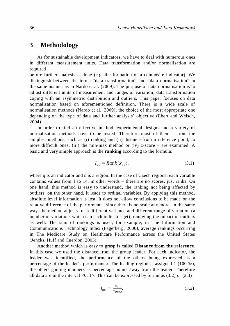
environmental pillars (see Figure 1) and reach their equilibrium state if possible.

The first sustainability measurement task is to select the proper indicators so

that the above pillars can be assessed adequately. In the Czech Republic, two main

attempts to evaluate regions from the sustainability point of view have been made

so far. The first one was aimed predominantly at the quality of life assessment

(Mederly et al., 2004). Despite having been targeted at the regional level (NUTS 3

and LAU 1 level4) as well, the first evaluation project did not provide an inspiration

3

As EUROSTAT defines, “The NUTS classification (Nomenclature of territorial units for

statistics) is a hierarchical system for dividing up the economic territory of the EU for the purpose

of the collection, development and harmonisation of EU regional statistics, socio-economic

analyses of the regions and framing of EU regional policies”. For more details see

http://epp.eurostat.ec.europa.eu/portal/page/portal/nuts_nomenclature/introduction . 4

Local Area Units (LAUs) were established by EUROSTAT to be compatible with NUTS

regions. For more details see

http://epp.eurostat.ec.europa.eu/portal/page/portal/nuts_nomenclature/local_administrative_units .

Transformation Methods and Sustainability Indicators in Czech Regions 33

Figure 1: Three most frequent sustainable development pillars.

to us since its outdated outcomes have been neither revised nor republished.

Another data source available is a statistical overview of sustainable indicators in

Czech NUTS 3 regions that is published irregularly, without a deeper analysis, by

the Czech Statistical Office. We decided to use the data from this source (Czech

Statistical Office, 2010) as a starting point of our research. The main obstacles

consist in the fact that – owing to irregular publishing (2007 and 2010) – it is not

easy to prolong the time series. Unlike the first approach, which used statistical

methods to analyse the relations and deeper coherence among 111 selected

indicators in the regions, the other one (Czech Statistical Office, 2010) did not use

any analytical tools to assess the inter-indicator relations, only the time series of

given indicators together with their basic characteristics (such as the mean,

variance or growth rate) having been published. We attempted to combine the

advantages of both approaches. Having selected the most up-to-date data from the

latter source, we performed a statistical analysis similar to that of Mederly et al.

(2004), the first step being the choice of a proper normalisation method.

Since we wanted to utilize the latest data, taking into account their potential

(anticipated) extension to the future, we had to adjust the indicator matrix,

considering that not all the indicators would fit the bill. Some of them are not

observed regularly every year, only a few values being available. Methodological

changes are rather frequent as well. Indicators whose values are collected for

diverse regional structures (i.e. regions different from those defined on NUTS 3

level) represent another example of necessary adaptation. There are four types of

indicators (apart from the unchangeable and unquestionable ones) requiring certain

adjustments. They are those

1. with shortened time series,

2. with estimated (missing) values,

3. that pose a problem,

4. that had to be discarded.


Table 1 shows the list of indicators ranked into the above mentioned groups

from the time series point of view. For more details about indicators’ adjustments

see Fischer et al. (2013).

In our research (based on 2010 data, see below), we decided to discard – apart

from the four above mentioned indicators – Quality of Surface Water and Political

Participation in Regional Councils indicators as well, due to the data

incomparability. Unlike Fischer et al. (2013), we included Women and Men in

Politics on the level of Municipal Councils indicator – because of good data

availability for the year 2010 – for this very kind of analysis.

The final set of indicators (after all changes made) is listed in Appendix 1. In

compliance with Figure 1, all the indicators are divided into three sustainable

development pillars – economic (13 indicators), social (15) and environmental (12).

For the comparison of normalisation methods employed in this research paper, the

most recent data period was chosen, only 2010 data being used.

First of all, having selected the indicators and determined their direction, we

performed a correlation coefficient analysis to check whether the inclusion of some

indicators is not useless. The evaluation has to be conducted from both a statistical

and practical perspective. A strong correlation between a general and registered

Table 1: List of indicators with certain adjustment procedures

1. Indicators with shortened time series

1. Households with Net Income below Subsistence Minimum

2. Organic Farming

3. Passenger Transport

2. Indicators with estimated (missing) values

1. Passenger Transport

2. Internet Access

3. Quality of Surface Water

4. Share of Broadleaved Species

5. Areas with Deteriorated Air Quality

6. Civil Society – Political Participation

3. Problematic indicators

1. Labour Productivity

2. General Government Deficit/Surplus

3. Coverage of the Czech Republic’s Territory by approved Town and Country

Documentation of Municipalities

4. Quality of Surface Water

5. Areas with Deteriorated Air Quality.

4. Discarded indicators

1. Registered Unemployment Rate

2. Average Duration of Court Proceedings

3. Women and Men in Politics

4. Index of Defoliation


unemployment rate was one of the reasons why we eliminated the latter from the

analysis. In some other cases, the correlation was spurious, i.e. the indicators were

left in the dataset.

As a case study, the Czech Republic NUTS 3 regions were used. NUTS 2 level,

usually employed in the European Union comparisons, proved to be less

favourable, because there are only eight of these regions in the Czech Republic,

artificially created as a connection of (one to three) NUTS 3 units. The application

of a lower level LAU 1 would make us use less common sustainable development

indicators, since it is not possible to measure economic indicators such as GDP per

capita at such a level. Therefore we selected 14 NUTS 3 regions (Figure 2).

In our opinion, sustainable development indicators form a good example,

because they can hardly ever be (irrespective of the author and selected indicators)

in the same measurement units, the choice of the proper method being indisputably

important.

Every data transformation and/or normalisation increases uncertainty and

measurement error probability. Therefore the assessment of advantages and

disadvantages of the chosen method is essential.

Figure 2: Czech Republic NUTS 3 regions. (Source: Czech Statistical Office, 2012,

authors’ adaptation)


3 Methodology

As for sustainable development indicators, we have to deal with numerous ones

in different measurement units. Data transformation and/or normalisation are

required

before further analysis is done (e.g. the formation of a composite indicator). We

distinguish between the terms “data transformation” and “data normalisation” in

the same manner as in Nardo et al. (2009). The purpose of data normalisation is to

adjust different units of measurement and ranges of variation, data transformation

coping with an asymmetric distribution and outliers. This paper focuses on data

normalisation based on aforementioned definition. There is a wide scale of

normalisation methods (Nardo et al., 2009), the choice of the most appropriate one

depending on the type of data and further analysis’ objective (Ebert and Welsch,

2004).

In order to find an effective method, experimental designs and a variety of

normalisation methods have to be tested. Therefore most of them – from the

simplest methods, such as (i) ranking and (ii) distance from a reference point, to

more difficult ones, (iii) the min-max method or (iv) z-score – are examined. A

basic and very simple approach is the ranking according to the formula:

, (3.1)

where q is an indicator and c is a region. In the case of Czech regions, each variable

contains values from 1 to 14, in other words – there are no scores, just ranks. On

one hand, this method is easy to understand, the ranking not being affected by

outliers, on the other hand, it leads to ordinal variables. By applying this method,

absolute level information is lost. It does not allow conclusions to be made on the

relative difference of the performance since there is no scale any more. In the same

way, the method adjusts for a different variance and different range of variation (a

number of variations which can each indicator get), removing the impact of outliers

as well. The sum of rankings is used, for example, in The Information and

Communications Technology Index (Fagerberg, 2000), average rankings occurring

in The Medicare Study on Healthcare Performance across the United States

(Jencks, Huff and Cuerdon, 2003).

Another method which is easy to grasp is called Distance from the reference.

In this case we used the distance from the group leader. For each indicator, the

leader was identified, the performance of the others being expressed as a

percentage of the leader’s performance. The leading region is assigned 1 (100 %),

the others gaining numbers as percentage points away from the leader. Therefore

all data are in the interval <0, 1>. This can be expressed by formulas (3.2) or (3.3)

, (3.2)


(3.3)

The results presented in the next section are derived from the formula (3.2)

adjusted according to the direction of the indicator. An alternative is to set the

value of the laggard region to 1. This guarantees that the transformed data are

higher than or equal to 1, which proves useful for further analysis, e.g. geometric

aggregation. The method adjusts different scales, having preserved relative

distances. It makes this technique easy to handle and understand, but the imbalance

between scores and rankings remains. The distance from the reference method,

however, tackles neither outliers nor different variance and range of variation. The

resulting indicators are less robust to the influence of outliers than other methods.

The impact of outliers and extreme values is determined by the reference. In the

case of a leader (or laggard), the method can be more prone to distorted results.

However, not only a group leader (or laggard) can serve as a reference. Also the

mean value, a target to be achieved in a given period of time, an external

benchmark or average (e.g. EU-27) can be used. It is necessary to add that the issue

becomes serious when the outliers are chosen as a reference. Examples of this

method are Eco-indicator 99, published by Pre Consultants (in the Netherlands),

and the Summary Innovation Index (SII), which uses the differences of sub-

indicator values from corresponding European averages (Saisana and Tarantola,

2002).

According to the Categorical scale method, a categorical score – either

numerical or qualitative – is assigned to each indicator. The most common are

three- or five-point scales (e.g. “agree”, “undecided”, “disagree”; or “strongly

agree”, “agree”, “undecided”, “disagree”, “strongly disagree”) or grade-based ones.

Thresholds have to be chosen for score assignments in different categories.

Categorical scales are prone to be highly subjective since they depend on a

subjective choice of thresholds which may be selected arbitrarily (Jacobs, Smith

and Goddard, 2004). A numerical scale can be expressed as [1, …, c], c > 1,

depending on whether the value is below or above a given threshold. Thus ,

observations (e.g. regions) are compared among themselves, not with a benchmark.

Usually it is based on percentiles of the distribution. For example, the top 10 %

gain a full score of 100, the observations between the 90th

and 75th

percentiles

receiving 80 points, those between the 75th

and 60th

percentiles 60 points, and so on

down to 0 points.

The simplest version is a method called Indicators above/below the mean. The

values close to the mean receive a zero, those above/below a given threshold

receive 1 and -1 respectively. Hence, this technique is basically a sub-model within

categorical scales, outcome values in question being only -1, 0 or 1. Despite its

subjective and arbitrary nature, category threshold setting remains a matter of

principle. The method is simple, not distorted by outliers, the main problem being a

significant loss of information compared to other methods such as min-max or z-

scores. For example, if the values of a given indicator for region A are two times


(200 %) above the mean, and the value for region B is 50 % above the mean, both

regions would be considered as “above the mean”, i.e. 1 unless the threshold is less

than 50 % above the mean. In other words, if the threshold is below the level of A

and B regions, both regions receive the same normalised value even if the former

performs significantly better. This may bring rather poor information which can

result in a misleading conclusion.

The method adjusts different scales, variance and range of variation as well as

outliers – all, however, at the expense of the loss of some important data properties.

There are not the same relative distances any more. It is clear that categorical

scales exclude large amounts of information about the original scale and variance

of transformed indicators, i.e. the original data distribution. There is another

problem with respect to the robustness of the results. On one hand, small year-to-

year changes do not affect the transformed variable since it remains in the same

class (category). On the other hand, these year-to-year changes are not captured in

the ranking system.

Since the creation and application of a categorical scale leads to a significant

loss of information, we express the original numbers in percentiles. Having not

used any categorical scales, we received an indicator value expressed as a relative

number reflecting the position of a particular region among all other regions. (The

applied method is labelled as “Scale” in the Result section of this paper.)

Composite indicators using categorical scales are, for example, Overall Health

System Achievement (Murray et al. 2001) or Regional Innovation Scoreboard 2012

(European Commission 2012).

Standardisation (or z-score method) converts data in order to get normal

distribution. Standardisation means that for each indicator , the average across

countries and standard deviation across countries are calculated and

used in the formula (3.4):

(3.4)

After performing standardisation, the data have a common scale with a zero

mean and standard deviation of 1. Since all z-score distributions have the same

mean and standard deviation, individual scores from different distributions can be

directly compared. This method’s advantage is that it provides no distortion from

the mean, adjusting for different scales and variance. The output is dimensionless ,

and due to the application of a linear transformation, the relative differences are

maintained. Although the method does not fully adjust for outliers, the minimum

and maximum values are not as influential as in any other method, e.g. that of the

distance from the reference. An extreme value indicator has a greater effect on a

composite indicator. It is desirable that an exceptional behaviour should be

rewarded if an excellent performance on a few indicators is considered to be better

than other average performances. This effect, however, can be reduced by applying

a proper aggregation method. Z-scores technique was used for measuring


Performance and Investment in the knowledge-based economy (both by DG RTD)

or assessing the relative intensity of regional problems in the Community by the

European Commission (Saisana and Tarantola, 2002).

The Min-max method rescales data into different intervals based on minimum

and maximum values. According to the original direction of a variable, the min-

max formula (3.5) or (3.6) is used:

(3.5)

, (3.6)

where is the value of indicator q for country c. The advantage is that the

boundaries can be set and all indicators get an identical range (0, 1). Each indicator

reaches a value between 0 and 1 even if it is an extreme one. The output is

dimensionless and relative distances remain constant. Nevertheless, a drawback

gets revealed if outliers and/or extreme values are presented. The method is based

on extreme values (minimum and maximum ones) which can be outliers. These two

values strongly influence the final output. Another disadvantage is that the different

variance is not fully eliminated. Compared to z-score, this method is even more

sensitive to outliers since it is based on the range (not on the standard deviation).

The above mentioned approach is very popular, having been applied for the

construction of many composite indicators. The most known composite indicator,

the Human Development Index (HDI), published yearly by the United Nations, is

based on this type of transformation (Klugman, 2011). The min-max normalisation

method was employed in the data transformation, for example, in the DEA analysis

when constructing a composite indicator (Cherchye et al., 2009).

The above list of selected transformation methods is not exhaustive. There are

multiple other methods, e.g. the whole Box-Cox family, where the main issue is to

estimate an unknown transformation parameter λ (Box and Cox, 1964, Lai, 2010).

If indicators have very skewed distributions, logarithmic transformations or

trimming can be done (Jacobs, Smith and Goddard, 2004). There are other methods

suitable for time series transformation (e.g. Ansley et al., 1977), such as those for

cyclical indicators, percentage of annual differences over time, time distance, etc.

The present paper does not focus on time series and progress in time measurements,

the data transformation for time-dependent studies being just briefly mentioned.

Therefore not even the methods used for building composite leading indicators are

paid attention to, only the normalisation method, as defined before, being dealt

with.

Rankings derived from the different normalisation methods are supposed to be

the same. Differences in values, however, exist. Thus, the follow-up operations

with indicators are affected by the chosen method. To demonstrate these results, a


simple example of linear aggregation is employed. The overall composite indicator

Yc is determined by the formula (3.7):

∑ (3.7)

where is the normalised indicator for the q sub-indicator and c region. In order

to give a very simple example, no weights (i.e. equal weights) were used. All

results have been computed in MS Excel environment.

4 Results

Apart from the selection of a suitable indicator, a very important (and rather

complicated) task is to determine its “direction” or optimal performance (Munda

and Saisana, 2011), i.e. to make a decision whether the maximum or minimum

value is required as the best one. In some cases, we found it difficult to decide; e.g.

for all types of freight transport taken together, neither maximum nor minimum

seems to be the convenient value. This is owing to the fact that growing freight

transport can be favourable to some regions, while not to others – depending on the

initial value. Moreover, the indicator includes all types of freight forwarding.

Whereas an increase in railway transport can be seen as generally positive, that in

road transport would be perceived as mostly negative.

The next phase was a descriptive analysis of the dataset along with the

identification of outliers. Since this usually concerns regions with the capital city, it

is also the case of Prague region (Hlavní město Praha). In seven indicators, the

Prague value was an outlier. In two other (environmental) indicators, Ústecký kraj

was identified as an outlier, because chemical and other heavy industries are

located there. The impact of outliers was reduced by the applied normalisation

methods.

The most important outcome, which cannot be obvious at the first sight, is that

having applied a normalisation method to the data, the normalised indicators

achieved the same ranking regardless the method employed. The regions’ rankings

according to the economic pillar are shown in Table 2. From the point of view of

this pillar, we can see that the regions with two biggest cities (Hlavní město Praha

and Jihomoravský kraj) perform very well in most of the indicators. The smallest

region – Karlovarský kraj, on the other hand, shows the worst results.

The rankings in the social pillar are indicated in Table 3. According to this

pillar, the situation is a little different. We obtained one clear “leader” – the capital

city region (Hlavní město Praha), and an obvious “outsider” – structurally affected

Ústecký kraj.


Table 2: Economic pillar rankings

Hla

vn

í m

ěsto

Pra

ha

Stř

edo

česk

ý

kra

j

Jih

oče

ský

kra

j

Plz

eňsk

ý k

raj

Kar

lov

arsk

ý

kra

j

Úst

eck

ý k

raj

Lib

erec

ký

kra

j

Krá

lov

éhra

dec

ký

kra

j

Par

dub

ick

ý

kra

j

Kra

j V

yso

čin

a

Jih

om

ora

vsk

ý

kra

j

Olo

mo

uck

ý

kra

j

Zlí

nsk

ý k

raj

Mo

rav

sko

slez

s

ký

kra

j

EC1 1 3 5 6 14 8 13 4 11 10 2 12 7 9 EC2 3 1 7 11 14 12 2 8 13 6 8 4 10 5 EC3 1 7 8 9 14 3 13 5 12 10 2 11 6 4 EC4 11 12 7 1 9 13 6 10 5 14 2 8 4 3 EC5 1 7 6 5 4 12 11 8 10 14 2 3 13 9 EC6 1 9 8 2 6 4 11 13 12 10 5 3 14 7 EC7 1 2 8 4 10 13 7 5 11 6 3 14 9 12 EC8 1 9 7 11 13 12 10 8 5 6 3 4 2 14 EC9 2 8 14 13 12 5 3 6 4 11 10 9 7 1 EC10 1 8 11 12 5 2 3 4 7 13 10 9 14 6 EC11 1 12 6 9 14 13 5 4 11 8 2 10 3 7 EC12 14 4 10 12 11 13 5 7 8 9 1 3 2 6 EC13 3 1 7 5 14 13 6 10 4 12 2 9 8 11

The rankings in the environmental pillar are described in Table 3. In this pillar, the

results vary the most of all the three pillars. Hlavní město Praha, unlike the two

previous pillars, is the worst performing region of all 14 regions. There is no clear

“leader” in this pillar.

Table 3: Social pillar rankings

Hla

vn

í m

ěst

o

Pra

ha

Stř

ed

očesk

ý

kra

j

Jih

očesk

ý k

raj

Plz

eň

ský

kra

j

Karl

ov

ars

ký

kra

j

Úst

eck

ý k

raj

Lib

ere

ck

ý

kra

j

Krá

lov

éh

rad

e

ck

ý k

raj

Pard

ub

ick

ý

kra

j

Kra

j V

yso

čin

a

Jih

om

ora

vsk

ý

kra

j

Olo

mo

uck

ý

kra

j

Zlí

nsk

ý k

raj

Mo

rav

sko

slez

ský

kra

j

SO1 3 5 8 2 4 14 9 6 6 1 10 12 11 13 SO2 1 2 3 4 13 14 7 5 8 6 9 11 10 12 SO3 1 2 8 4 3 12 5 9 7 10 6 13 11 14 SO4 1 3 5 4 2 14 10 8 9 7 6 13 11 12 SO5 2 3 7 9 7 13 1 5 10 3 5 12 10 13 SO6 1 9 6 4 12 14 8 2 5 3 7 10 11 13 SO7 1 9 7 11 13 14 10 5 6 2 3 8 4 12 SO8 1 5 7 8 14 13 12 9 10 11 2 4 3 6 SO9 1 5 13 4 7 11 14 3 6 10 2 12 8 9 SO10 7 14 5 1 3 12 11 6 10 13 2 4 9 8 SO11 1 11 9 14 13 8 12 7 4 10 5 3 6 2 SO12 11 4 6 8 14 13 10 5 2 1 7 9 3 12 SO13 1 6 7 10 14 13 11 4 3 2 8 9 5 12 SO14 13 2 12 11 5 1 3 8 7 14 9 4 10 6 SO15 1 10 2 3 11 12 7 5 6 4 9 8 13 14


Table 4: Environmental pillar rankings

Hla

vn

í m

ěsto

Pra

ha

Stř

edo

česk

ý

kra

j

Jih

oče

ský

kra

j

Plz

eňsk

ý k

raj

Kar

lov

arsk

ý

kra

j

Úst

eck

ý k

raj

Lib

erec

ký

kra

j

Krá

lov

éhra

dec

ký

kra

j

Par

dub

ick

ý

kra

j

Kra

j V

yso

čin

a

Jih

om

ora

vsk

ý

kra

j

Olo

mo

uck

ý

kra

j

Zlí

nsk

ý k

raj

Mo

rav

sko

slez

s

ký

kra

j

EN1 10 14 5 7 1 6 2 8 9 12 13 11 4 3 EN2 14 11 7 3 2 5 1 10 8 6 9 13 12 4 EN3 14 13 3 5 2 9 1 7 10 11 12 8 4 6 EN4 14 13 6 8 1 5 2 9 11 10 12 7 4 3 EN5 1 7 13 12 11 4 9 8 10 14 2 5 3 6 EN6 14 10 5 6 3 9 7 4 2 1 8 11 12 13 EN7 14 10 1 3 9 13 2 4 11 5 8 7 6 12 EN8 12 9 5 8 11 14 4 6 10 1 2 3 7 13 EN9 14 7 10 12 1 9 3 5 4 2 11 6 8 13 EN10 5 14 13 1 7 9 3 2 12 8 4 10 6 11 EN11 8 6 3 10 12 2 9 13 7 11 1 14 4 5 EN12 13 3 8 9 10 1 2 5 12 14 7 11 6 4

The transformed indicators were used in order to get a composite indicator. They

were aggregated by means of the average of the values of sub-indicators. It implies

that the values of transformed indicators themselves – not their rankings – were

used in the formula 3.7. Table 5 shows region rankings based on the values of

composite indicators.

The same details as in Table 5 are depicted in Figure 3. They clearly show the

difference in region rankings resulting from the chosen normalisation method. In

the case of a leader (Hlavní město Praha) and laggard (Ústecký kraj), the chosen

normalisation method does not matter. But in the other regions, differences can be

significant. The Distance from a reference method seems to be the least consistent

with the other ones. Kraj Vysočina, for instance, is ranked 5th

by the distance from

the reference method but 10th

by the other ones.

Table 5: Overall rankings by means of different techniques

Hla

vn

í m

ěsto

Pra

ha

Stř

edo

česk

ý k

raj

Jih

oče

ský

kra

j

Plz

eňsk

ý k

raj

Kar

lov

arsk

ý k

raj

Úst

eck

ý k

raj

Lib

erec

ký

kra

j

Krá

lov

éhra

dec

ký

kra

j

Par

dub

ick

ý k

raj

Kra

j V

yso

čin

a

Jih

om

ora

vsk

ý

kra

j

Olo

mo

uck

ý k

raj

Zlí

nsk

ý k

raj

Mo

rav

sko

slez

ský

kra

j

Min-max 1 6 8 4 12 14 3 5 7 10 2 11 9 13

Z-score 1 6 7 4 12 14 3 5 8 10 2 11 9 13

Rank 1 7 6 5 12 14 4 3 9 10 2 11 8 12

Distance from a reference 1 11 7 4 6 14 2 8 10 5 3 12 9 13

Scale 1 7 6 5 12 14 4 3 9 10 2 11 8 13


0123456789

1011121314

Hlavní město Praha

Středočeský kraj

Jihočeský kraj

Plzeňský kraj

Karlovarský kraj

Ústecký kraj

Liberecký kraj

Královéhradecký kraj

Pardubický kraj

Kraj Vysočina

Jihomoravský kraj

Olomoucký kraj

Zlínský kraj

Moravskoslezský kraj

Max-min Z score Rank Distance from a reference Scales

Figure 3: Overall rankings by means of different techniques.

In order to assess the relation between normalisation methods, Spearman

correlation coefficients were computed. The correlation coefficient close to 1

implies that the rankings of the majority of regions remain unchanged when

different methods are applied. The results in Table 6 indicate that the Scale and

Rank are basically the same (compare with Figure 3). Let us bear in mind,

however, that the Scale technique provides also relative values, not just the rank.

Table 6: Spearman correlation (in %)

Min-max Z-score Rank

Distance

from the

reference Scale

Min-max 100.0 87.5 75.9 49.4 76.0

Z-score 87.5 100.0 93.9 47.5 93.9

Rank 75.9 93.9 100.0 46.0 100.0

Distance from a reference 49.4 47.5 46.0 100.0 45.7

Scale 76.0 93.9 100.0 45.7 100.0


Rather low correlations between the Distance from the reference technique and the

other methods confirm the above mentioned results. High correlations (above 75

%), on the other hand, occur among the remaining methods, the results being very

similar.

5 Discussion and conclusions

In the paper, we deal only with data normalisation methods, which are commonly

used for building composite indicators. Having ignored other types of data

transformation, we focused on the normalisation method and its usefulness in

particular. A sound experimental design was created and implemented in order to

generate adequate statistical data. Various normalisation techniques having been

scrutinized, we assessed the data normalisation effects on the final rankings, being

aware that different methods might produce different outcomes. Data

characteristics and project objectives (those of composite indicators´ construction,

in this very case) have to be taken into account in the method selection process.

Two main issues were raised: namely, whether (i) the extreme values ought to be

rewarded or penalised (as an exceptional behaviour) and whether (ii) the scores for

normalised indicators should be kept. According to the answers, the proper method

is to be selected.

Our case study was aimed at sustainability indicators in Czech NUTS 3 regions.

Although the regions are still assessed mainly according to the regional GDP per

capita or unemployment rate in the Czech Republic, sustainable development

remains a lively theoretical issue. Also practical attempts to launch regional

sustainability strategies have been made (e.g. in the regions of Ústecký kraj and

Liberecký kraj). The prospect that sustainable development indicators (and their

trends) will soon become the regional assessment criteria seems reasonable.

However, the general consensus on how to measure sustainable development has

not been reached yet. One of the most debated approaches is measurement via a

composite indicator. As soon as a political decision on the use of the sustainable

development composite indicator is made, the need to select the proper

normalisation method will become urgent. This paper attempts to address this

crucial issue since the chosen normalisation method itself can principally influence

the final output of a composite indicator.

Having compared all applied techniques, it appeared that the Distance from the

reference method (the regional leader being chosen as the reference) produced the

most diverse results of all. Each method has its advantages and disadvantages. A

particular normalisation method cannot suit all kinds of analyses, having significant

effects on the construction of the composite indicator. Therefore it is up to the

indicator designer to choose the most appropriate method. Its choice has to be well-

grounded and justifiable, sensitivity and uncertainty analysis being an integral part

of the composite indicator construction process.


Acknowledgement

This paper has been prepared under the support of the University of Economics in

Prague, project No. 11/2012 “Construction and verification of sustainable

development indicators in the Czech Republic and its regions”. The authors would

like to thank two anonymous referees for their valuable comments.

References

[1] Ansley, C.F., Spivey, W.A. and Wrobleski, W.J. (1977): A Class of

Transformations for Box-Jenkins Seasonal Models. Journal of the Royal

Statistical Society: Series C (Applied Statistics), 26, 173-178.

[2] Blanc, I., Friot, D., Margni, M. and Jolliet, O. (2008): Towards a new index

for environmental sustainability based on a DALY weighting approach.

Sustainable Development, 16, 251-260.

[3] Box, G.E.P. and Cox, D.R. (1964): An Analysis of Transformations. Journal

of the Royal Statistical Society. Series B (Methodological) , 26, 211-252.

[4] Czech Statistical Office. (2010): Vybrané oblasti udržitelného rozvoje v

krajích České republiky 2010. Praha: Český statistický úřad.

[5] Czech Statistical Office (2012): Oblasti (NUTS 2) a kraje (NUTS 3) České

republiky [online].

<http://www.czso.cz/csu/redakce.nsf/i/oblasti_%28nuts_2%29_a_kraje_%28n

uts_3%29_ceske_republiky>. [cit. 3 Feb 2012].

[6] Czesaný, S. (2006): Indikátory udržitelného rozvoje. Statistika, 43, 431-434.

[7] Ebert, U. and Welsch, H. (2004): Meaningful environmental indices: a social

choice approach. Journal of Environmental Economics and Management, 47,

270-283.

[8] European Commission (2012): Regional Innovation Scoreboard 2012.

European Commission.

[9] Fagerberg, J. (2000): Europe at the Crossroads: The Challenge from

Innovation-based Growth. Presented at the ERC/METU International

Conference in Economics IV, September 13-16, Ankara, Turkey.

[10] Fischer, J., Helman, K., Kramulová, J., Petkovová, L. and Zeman, J. (2013):

Sustainable development indicators at the regional level in the Czech

Republic. Statistika, 93, 5-18.

[11] Freudenberg, M. (2003): Composite Indicators of Country Performance: A

Critical Assessment. OECD Science, Technology and Industry Working

Papers, 2003/16. Paris: OECD Publishing.

[12] Cherchye, L., Moesen, W., Rogge, N. and Van Puyenbroeck, T. (2009):

Constructing a knowledge economy composite indicator with imprecise data.

CES-Discussion paper series, 09.15, 1-24.


[13] Jacobs, R., Smith, P. and Goddard, M.K. (2004): Measuring performance: an

examination of composite performance indicators: a report for the Department

of Health. York: Centre of Health Economics, University of York.

[14] Jencks, S.F., Huff, E.D., and Cuerdon, T. (2003): Change in the quality of care

delivered to Medicare beneficiaries, 1998-1999 to 2000-2001. JAMA: the

journal of the American Medical Association , 289, 305-312.

[15] Klugman, J. (2011): Human Development Report 2011. Sustainability and

Equity: A Better Future for All. New York: United Nations Development

Programme.

[16] Lai, D. (2010): Box-Cox Transformation for Spatial Linear Models: A Study

on Lattice Data. Statistical Papers, 51, 853-64.

[17] Macháček, J. (2004): Ekonomické souvislosti využívání kulturně historických

lokalit. Praha: Oeconomica.

[18] Mederly, P., Topercer, J. and Nováček, P. (2004): Indikátory kvality života a

udržitelného rozvoje – kvantitativní, vícerozměrný a variantní přístup. Praha:

UK FSV CESES.

[19] Munda, G. and Saisana, M. (2011): Methodological Considerations on

Regional Sustainability Assessment Based on Multicriteria and Sensitivity

Analysis. Regional Studies, 45, 261-276.

[20] Nardo, M., Saisana, M., Saltelli, A., Tarantola, S., Hoffman, H. and

Giovannini, E. (2009): Handbook on constructing composite indicators:

methodology and user guide. Paris: Organisation for Economic Co-operation

and Development.

[21] Murray, C.J.L., Lauer, J., Tandon, A. and Frenk, J. (2001): Overall health

system achievement for 191 countries. EIP/GPE Discussion Paper Series, 28.

World Health Organization.

[22] Nováček, P. and Mederly, P. (1996): Strategie udržitelného rozvoje. Praha: G

plus G.

[23] OECD (2002): Aggregated Environmental Indices: Review of Aggregation

methodologies in use. Paris: OECD Working Group on Environmental

Information and Outlooks.

[24] Saisana, M. and Tarantola S. (2002): State-of-the-art report on current

methodologies and practices for composite indicator development . Ispra:

Institute for the Protection and the Security of the Citizen Technological and

Economic Risk Management Unit.


Appendix 1 - Final set of indicators after all changes

Economic pillar

EC1 Gross Domestic Product per Capita in thousands of CZK (current prices)

EC2 Change in Gross Domestic Product (Development of GDP in constant prices)

EC3 Labour Productivity (Development of GDP per 1 employed)

EC4 Local Government Deficit/Surplus

EC5 Gross Value Added in Services (Share of the Tertiary Sector in Gross Value

Added in %)

EC6 Investment Rate in %

EC7 Net Disposable Income of Households per inhabitant in thousands of CZK

EC8 Small and Medium-sized Enterprises (Share of Small and Medium-sized

Enterprises in the Total Employment in %)

EC9 Transport Infrastructure – Density of the Motorway Network in km per 100 km2

EC10 Transport Infrastructure – Railway Lines Density in km per 100 km2

EC11 Freight Transport (Excluding Transit, including Road, Rail and Water Transport

per thousand of CZK GDP, in kg)

EC12 Passenger Transport (within the Region by Public Road and Rail Transport per

Capita)

EC13 Research & Development Expenditures to GDP in % Source: Czech Statistical Office, 2010, authors’ adaption


Social pillar

SO1 Households with Net Income below Subsistence Minimum

SO2 General Unemployment Rate in % (Aged 15+)

SO3 Employment of Elderly Workers (Employment Rate of People Aged 55-64 in %)

SO4 Employment of Women in %

SO5 Mortality (Standardised Mortality Rate - Number of Deaths per 1000 mid-year

Population)

SO6 Life Expectancy (of men at birth in years)

SO7 Life Expectancy (of women at birth in years)

SO8 Highest Level of Education Attained (Share of the Population with Tertiary

Education in the Population Aged 15 and Over in %)

SO9 Internet Access (Share of Households connected to Internet in %

SO10 Local Government Expenditures on Culture per inhabitant in CZK

SO11 Coverage of the Czech Republic's Territory by Approved Town and Country

Documentation of Municipalities in %

SO12 Civil Society – Political Participation (Turnout in Elections to Municipal Councils

in %)

SO13 Civil Society – Political Participation (Turnout in Elections to the Chamber of

Deputies in %)

SO14 Women and Men in Politics (Share of the Total Number of Women Elected

Representatives in Elections to Municipal Councils in %)

SO15 Civil Society – Civil Participation (Mid-year Population to Non-profit

Organization) Source: Czech Statistical Office, 2010, authors’ adaption

Environmental pillar

EN1 Arable Land in %

EN2 Consumption of Industrial Fertilizers in Pure Nutrients in kg/ha of Arable Land

EN3 Coefficient of Ecological Stability

EN4 Organic Farming (Share of organically farmed land in the total area of agricultural

land in %

EN5 Share of Broadleaved Species in %

EN6 Areas with Deteriorated Air Quality in %

EN7 Nitrogen Oxide Emissions (REZZO 1-4) in tonne per km2

EN8 Sulphur Dioxide Emissions (REZZO 1-3) in tonne per km2

EN9 Waste Generated by Enterprises in kg per thousand CZK of GDP

EN10 Municipal Waste Generated in kg per inhabitant

EN11 Acquired Investment Expenditures on Environment Protection according to

Location of Investment in CZK per inhabitant

EN12 Non-investment Expenditures on Environment Protection according to Region of

Residence of the Investor per million CZK of Regional GDP Source: Czech Statistical Office, 2010, authors’ adaption

Documents

Transformation Methods and Sustainability Indicator … · advantages and disadvantages and compares the ... Transformation Methods and Sustainability ... Politics on the level of