Rochester Institute of TechnologyRIT Scholar Works

Presentations and other scholarship Faculty & Staff Scholarship

9-30-2016

Transfer Learning for High Resolution Aerial ImageClassificationYilong Liang

Sildomar T. Monteiro

Eli S. Saber

Follow this and additional works at: https://scholarworks.rit.edu/other

This Conference Paper is brought to you for free and open access by the Faculty & Staff Scholarship at RIT Scholar Works. It has been accepted forinclusion in Presentations and other scholarship by an authorized administrator of RIT Scholar Works. For more information, please contactritscholarworks@rit.edu.

Recommended CitationY. Liang, S.T. Monteiro, E.S. Saber "Transfer Learning for High Resolution Aerial Image Classification," IEEE Applied Imagery PatternRecognition (AIPR) Workshop 2016, Washington, DC, October 2016. arXiv:1510.00098v2

Transfer Learning for High Resolution Aerial ImageClassification

Yilong Liang∗, Sildomar T. Monteiro∗†, Eli S. Saber∗†∗Chester F. Carlson Center for Imaging Science

†Department of Electrical and Microelectronic EngineeringRochester Institute of Technology, Rochester, NY, 14623

Email: {yxl7245, sildomar.monteiro, esseee}@rit.edu

Abstract—With rapid developments in satellite and sensortechnologies, increasing amount of high spatial resolution aerialimages have become available. Classification of these imagesare important for many remote sensing image understandingtasks, such as image retrieval and object detection. Meanwhile,image classification in the computer vision field is revolutionizedwith recent popularity of the convolutional neural networks(CNN), based on which the state-of-the-art classification resultsare achieved. Therefore, the idea of applying the CNN for highresolution aerial image classification is straightforward. However,it is not trivial mainly because the amount of labeled images inremote sensing for training a deep neural network is limited.As a result, transfer learning techniques were adopted for thisproblem, where the CNN used for the classification problem ispre-trained on a larger dataset beforehand. In this paper, wepropose a specific fine-tuning strategy that results in better CNNmodels for aerial image classification. Extensive experiments werecarried out using the proposed approach with different CNNarchitectures. Our proposed method shows competitive resultscompared to the existing approaches, indicating the superiorityof the proposed fine-tuning algorithm.

I. INTRODUCTION

Recently, the remote sensing images have been obtainedwith increasing spatial and spectral resolutions. The expansionof the spectral domain advances the spectral-related appli-cations, such as material identification. Meanwhile, the theincrease in spatial resolution makes the spatial details and tex-tures of the scenes more discernible. Recently, the WorldView-3 satellite sensor provides the images with panchromaticresolution of 0.31m, under which the territorial structures ofthe scene are accurately captured in the image. Classificationof high spatial resolution remote sensing images refers to as-signing semantic labels to recognize the images. The problemhas become an ongoing research topic in the past decadesdue to the the significant role it plays in facilitating manyapplications such as vegetation monitoring in agriculture,airport security and aviation safety operation in surveillance,land cover change detection in environmental monitoring, andso on.

Within the literature, a large amount of research effortshave been devoted to the image classification problem, fo-cusing on the design of better feature representations of theimages. These image representations ranges from low-levelones, such as color autocorrelogram (ACC) [1] and localcolor histogram (LCH) [2], to mid-level variants, such as bag

of visual words (BoW), and to high-level features that areautomatically learned from the image dataset [3]. Recently,deep learning techniques, especially the convolutional neuralnetworks (CNNs), have been applied for image classificationin computer vision areas and astounding classification resultswere achieved. One of the major advantages of applying theCNN approach in computer vision applications is that a largedataset containing millions of labeled images is available fortraining a robust deep CNN architecture. However, much fewerlabeled high resolution aerial images are available. As a result,different transfer learning techniques were adopted in order toapply the CNN approach to classify these images. Transferlearning refers to the technique that pre-trains a deep CNNmodel on a large but different dataset and then adapts thetrained model to specific problems where much smaller imagedatasets are available.

In this paper, we explore the transfer learning techniquesfor recognizing the high resolution aerial imagery. First, weextract image features using different pre-trained CNN archi-tectures trained using the ImageNet challenge dataset [4] andlearn new classifiers for recognizing our images. Next, wefine-tune the pre-trained CNNs to make the neural networkbetter adapt the aerial imagery. The proposed method wasdemonstrated to classify the images from the land use landcover (LULC) image dataset [5]. Our contributions include: (1)extract different features using various state-of-the-art CNNarchitectures for aerial image classification, (2) propose abetter fine-tuning framework for remote sensing aerial imagerywith small datasets, and (3) perform a comparative study ondifferent transfer learning techniques to better understand theCNN based image features.

II. RELATED WORK

Image classification has been thoroughly studied in thecomputer vision field and many algorithms have been pro-posed to solve this problem. Compared to computer visionapplications, classification of the aerial images are more chal-lenging given different appearances of the objects randomlyrotated within the scene and increasing complexities of thebackground textures. Initially, the problem was addressed withthe bag of word (BoW) model, which extracts image featuresusing the histograms of visual words derived from low levelfeatures in the images [5]. However, the BoW model does

not take the spatial relations between these visual words intoaccount and some research efforts have be devoted towardsincluding the spatial context information into the existingmodel. For example, authors in [5] proposed two algorithmsfor this purpose: (1) Adopt the spatial pyramid matching kernel(SPMK) introduced by Lazebinik et al. [6] to construct a three-layer pyramid of the image. The image is then represented asa vector concatenated from the BoW representations of thesepyramids. (2) Incorporate the co-occurrence kernel (SCK) withthe BoW model to compensate for the spatial information.However, as pointed out by Chen et. al. [7], the SCK-BoW iscomputational infeasible if the number of the visual words islarge. Therefore, the author proposed the pyramid of spatialrelaton (PSR) model to capture both absolute and relativespatial relationships between local features.

The major disadvantage of the algorithms based on BoWmodel is that hand-craft low level features, such as SIFT,are required to generate the discriminate descriptors. In orderto address this problem, many supervised and unsupervisedlearning methods have been studied to derive image featuresfrom the datasets. On one hand, unsupervised feature learningmethods are proposed to learn feature extractors from theimage scenes [8], [9]. On the other hand, tremendous pro-gresses have been made on supervised feature learning owingto the development of convolutional neural networks. Thegroundbreaking work of AlexNet proposed by Krizhevsky etal. [10] learns the image features with a eight-level deep neuralnetwork, which consists of five convolution layers and threefully connected layers, using ImageNet [11] consisting of 1000image categories. The success of the AlexNet lies in severaltricks introduced during training, including the applicationof rectified linear layer, the addition of the “dropout” layer,and the deployment of multiple GPUs. Ever since then, thereis an ongoing interest to learn deep CNN architectures forimage recognition. Better performances were achieved usingother CNN architectures, such as VGG [12], GoogleNet [13],and ResNet [14]. Results from these CNN based algorithmsindicate that the more layers the neural network contains,the better results it obtains. However, issues regarding todesigning these deep neural network arise as well, leading tomany simplification methods of filters to make sure the CNNarchitectures work properly.

In order to adapt the CNNs for the aerial image classifica-tion, one possible approach is to apply the pre-trained CNNmodels from the large image dataset, such as ImageNet, toextract features. The first attempt to apply the pre-trained CNNarchitectures on classifying high resolution aerial images wasdemonstrated in [3], where the pre-trained neural networks ofAlexNet and Overfeat [15] were adopted as feature extractors,and the activation maps form the second last layers of theCNN models were used for image representations. Later on,Castelluccio et. al. [16] proposed to fine-tune the weights ofthe convolution layers of the pre-trained CNNs to achievebetter image features. In order to make use of the outputsfrom mid-level layers of the CNN, Hu et. al. [17] proposedfeatures that aggregate the outputs from mid-level layers and

last fully connected layers of the CNN structure with featurecoding algorithms, showing improvement on the classificationresults.

III. METHODS

A. Convolutional Neural Networks

The convolutional neural networks (CNNs) provide end-to-end solutions for many image related tasks, such as imagesegmentation, recognition, and object detection. Usually, thearchitecture of a CNN model refers to the structure thatcontains a sequence of different layers concatenated one nextto the other. Each layer is characterized with neurons thatperform different differentiable mathematical operations, soas to make the neurons learn-able through back-propagation.In general, typical layers include the convolutional (CONV)layer, the pooling (POOL) layer, the rectified linear layer(ReLU), the fully connected (FC) layer, and the softmax(SOFTMAX) layer. The CONV layer contains a bank of threedimensional filters that convolve over the whole input data andoutputs a data cube that concatenates different filter outputstogether. The POOL layer aims at reducing the spatial size ofinput feature map with different down-sampling techniques,such as averaging and taking the maximum of local regionsof the input. In the FC layer, each neuron is connected toall the output neurons of the previous layer. Therefore, itcan be recognized as a special case of convolutional layerwhose receptive field covers the entire spatial region of itsinput. Finally, the SOFTMAX layer is connected to the lastFC layer to generate the classification score. In practise, thedeep CNN contains many layers and, therefore, the numberof learning parameters grows significantly, which leads to thepossibility of long training time and data over-fitting. As aresult, multiple approaches were proposed to mitigate theseproblems. For example, the drop out layer (DROP) is used torandomly drop a pre-defined portion of the parameters in thefilters and the batch normalization (NORM) is introduced tonormalize each channel of the feature map by averaging overspatial locations with a number of instances.

B. Existing CNN architectures for image classification

Based on various combinations of CNN layers with differentparameters, a variety of CNN architectures were derived. Inthis section, four CNN architectures are briefly discussed:AlexNet [10], VGG-F [12], GoogleNet [13], and ResNet[14]. These pre-trained CNN architectures were trained onthe ImageNet [11] dataset that contains over hundreds ofthousands of images with 1000 classes.

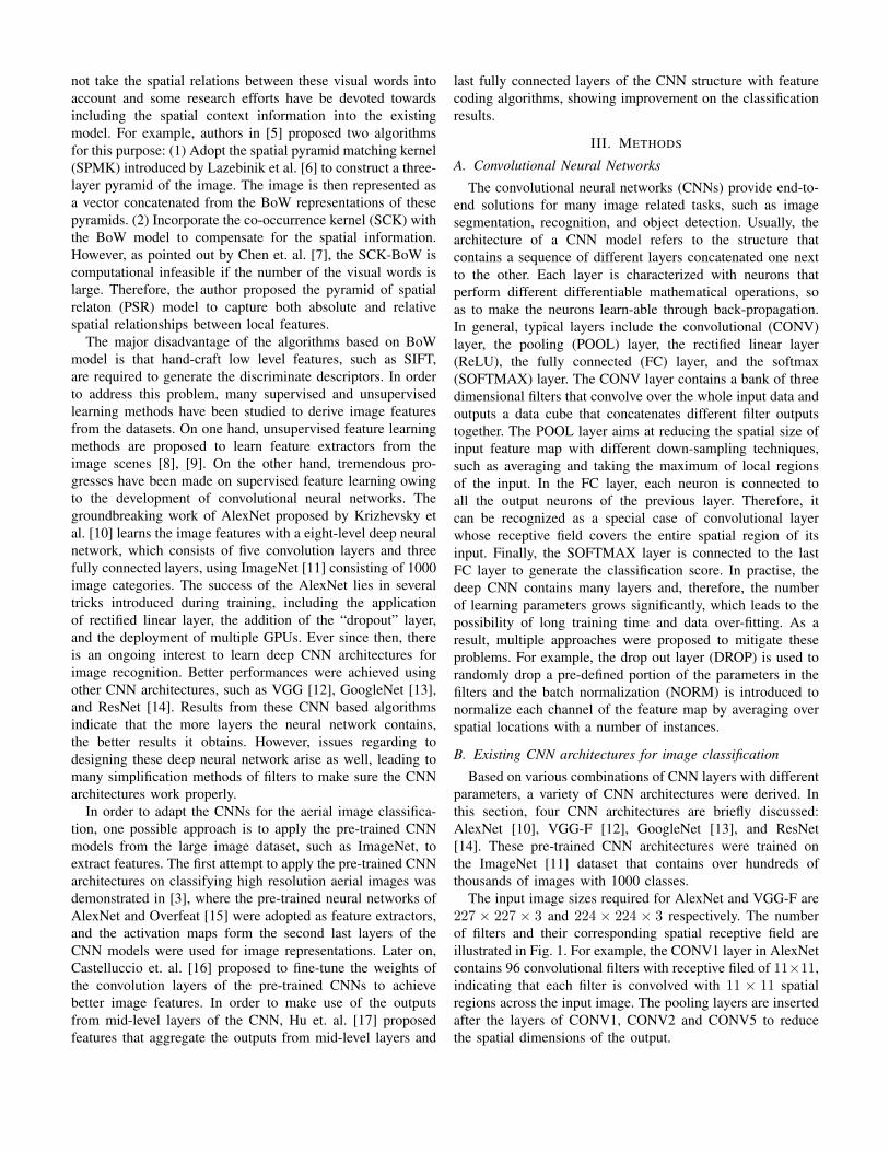
The input image sizes required for AlexNet and VGG-F are227 × 227 × 3 and 224 × 224 × 3 respectively. The numberof filters and their corresponding spatial receptive field areillustrated in Fig. 1. For example, the CONV1 layer in AlexNetcontains 96 convolutional filters with receptive filed of 11×11,indicating that each filter is convolved with 11 × 11 spatialregions across the input image. The pooling layers are insertedafter the layers of CONV1, CONV2 and CONV5 to reducethe spatial dimensions of the output.

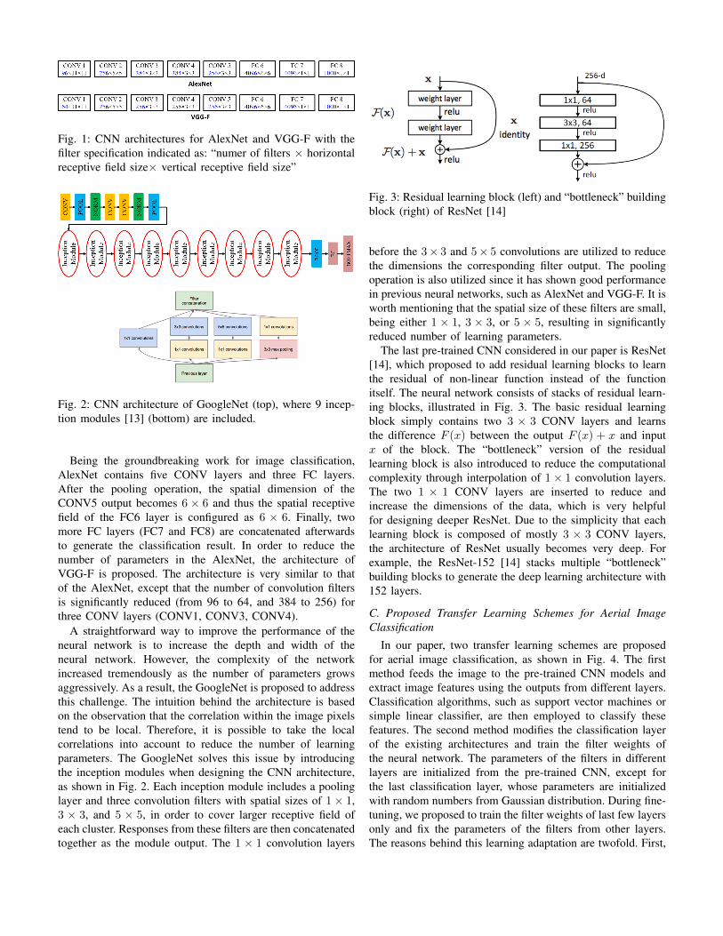
Fig. 1: CNN architectures for AlexNet and VGG-F with thefilter specification indicated as: “numer of filters × horizontalreceptive field size× vertical receptive field size”

Fig. 2: CNN architecture of GoogleNet (top), where 9 incep-tion modules [13] (bottom) are included.

Being the groundbreaking work for image classification,AlexNet contains five CONV layers and three FC layers.After the pooling operation, the spatial dimension of theCONV5 output becomes 6 × 6 and thus the spatial receptivefield of the FC6 layer is configured as 6 × 6. Finally, twomore FC layers (FC7 and FC8) are concatenated afterwardsto generate the classification result. In order to reduce thenumber of parameters in the AlexNet, the architecture ofVGG-F is proposed. The architecture is very similar to thatof the AlexNet, except that the number of convolution filtersis significantly reduced (from 96 to 64, and 384 to 256) forthree CONV layers (CONV1, CONV3, CONV4).

A straightforward way to improve the performance of theneural network is to increase the depth and width of theneural network. However, the complexity of the networkincreased tremendously as the number of parameters growsaggressively. As a result, the GoogleNet is proposed to addressthis challenge. The intuition behind the architecture is basedon the observation that the correlation within the image pixelstend to be local. Therefore, it is possible to take the localcorrelations into account to reduce the number of learningparameters. The GoogleNet solves this issue by introducingthe inception modules when designing the CNN architecture,as shown in Fig. 2. Each inception module includes a poolinglayer and three convolution filters with spatial sizes of 1× 1,3 × 3, and 5 × 5, in order to cover larger receptive field ofeach cluster. Responses from these filters are then concatenatedtogether as the module output. The 1 × 1 convolution layers

Fig. 3: Residual learning block (left) and “bottleneck” buildingblock (right) of ResNet [14]

before the 3× 3 and 5× 5 convolutions are utilized to reducethe dimensions the corresponding filter output. The poolingoperation is also utilized since it has shown good performancein previous neural networks, such as AlexNet and VGG-F. It isworth mentioning that the spatial size of these filters are small,being either 1 × 1, 3 × 3, or 5 × 5, resulting in significantlyreduced number of learning parameters.

The last pre-trained CNN considered in our paper is ResNet[14], which proposed to add residual learning blocks to learnthe residual of non-linear function instead of the functionitself. The neural network consists of stacks of residual learn-ing blocks, illustrated in Fig. 3. The basic residual learningblock simply contains two 3 × 3 CONV layers and learnsthe difference F (x) between the output F (x) + x and inputx of the block. The “bottleneck” version of the residuallearning block is also introduced to reduce the computationalcomplexity through interpolation of 1× 1 convolution layers.The two 1 × 1 CONV layers are inserted to reduce andincrease the dimensions of the data, which is very helpfulfor designing deeper ResNet. Due to the simplicity that eachlearning block is composed of mostly 3 × 3 CONV layers,the architecture of ResNet usually becomes very deep. Forexample, the ResNet-152 [14] stacks multiple “bottleneck”building blocks to generate the deep learning architecture with152 layers.

C. Proposed Transfer Learning Schemes for Aerial ImageClassification

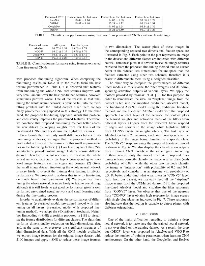
In our paper, two transfer learning schemes are proposedfor aerial image classification, as shown in Fig. 4. The firstmethod feeds the image to the pre-trained CNN models andextract image features using the outputs from different layers.Classification algorithms, such as support vector machines orsimple linear classifier, are then employed to classify thesefeatures. The second method modifies the classification layerof the existing architectures and train the filter weights ofthe neural network. The parameters of the filters in differentlayers are initialized from the pre-trained CNN, except forthe last classification layer, whose parameters are initializedwith random numbers from Gaussian distribution. During fine-tuning, we proposed to train the filter weights of last few layersonly and fix the parameters of the filters from other layers.The reasons behind this learning adaptation are twofold. First,

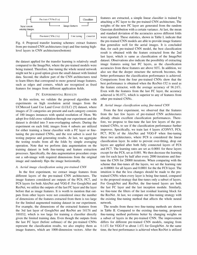
Fig. 4: Proposed transfer learning schemes: extract featuresfrom pre-trained CNN architectures (top) and fine-tuning high-level layers in CNN architectures(bottom)

the dataset applied for the transfer learning is relatively smallcompared to the ImageNet, where the pre-trained models werebeing trained. Therefore, fine-tuning the whole neural networkmight not be a good option given the small dataset with limiteddata. Second, the shallow part of the CNN architectures tendto learn filters that correspond to more general image features,such as edges and corners, which are recognized as fixedfeatures for images from different application fields.

IV. EXPERIMENTAL RESULTS

In this section, we validate the proposed algorithm withexperiments on high resolution aerial images from theUCMerced Land Use Land Cover (LULC) [5] dataset, whereimages of 21 categories are present and each category consistsof 100 images instances with spatial resolution of 30cm. Weadopt five-fold cross validation through our experiment and thedataset is divided into 5 non-overlapping subsets. During theexperiment on each fold, images from 4 subsets are utilizedfor either training a linear classifier with a FC layer or fine-tuning the pre-trained CNNs, and the rest subset is used fortesting purpose and generating results. At last, we aggregatethe testing results from all the folds by simple averagingoperation. Note that we perform data augmentation on thetraining dataset in both fine-tuning and feature extractionprocesses. Specifically, the data augmentation procedure cropsout a sub-image with required dimensions from the originalimage and randomly flips the image horizontally.

A. Aerial image classification using pre-trained CNN

In the first experiment, we extract image features fromdifferent layers of the pre-trained CNN architectures. Theimage features considered are outputs of the FC6, FC7, andFC8 layers for both AlexNet and VGG-F. For GoogleNet andResNet, we utilize the outputs of the last FC layer and the layerbefore that as image features. It is worth to mention that out-puts from other layers were not considered since the numberof dimensions of the features extracted from them is too largefor the limited augmented training dataset in our experiment.For example, the dimensions of the extracted features fromthe 3rd last layer of GoogleNet and ResNet are 50176 and100352, which is too large for training a classifier directlygiven the limited training data. Even though the outputs fromthe last FC layer (before softmax) of the pre-trained CNNsrepresent the classification results, we also employ them asimage features, which are 1000-dimension vectors. After the

features are extracted, a simple linear classifier is trained byattaching a FC layer to the pre-trained CNN architecture, Theweights of the new FC layer are generated from the randomGaussian distribution with a certain variance. At last, the meanand standard deviation of the accuracies across different foldswere reported. These statistics, shown in Table I, indicate thatthe pre-trained CNN models are able to provide image featuresthat generalize well for the aerial images. It is concludedthat, for each pre-trained CNN model, the best classificationresult is obtained with the feature extracted from the 2ndlast layer, which is same as classification of the ImageNetdataset. Observations also indicate the possibility of extractingimage features using last FC layers, as the classificationaccuracies from these features are above 93%. In addition, wealso see that the deeper structure the network becomes, thebetter performance the classification performance is achieved.Comparisons from the four pre-trained CNNs show that thebest performance is obtained when the ResNet-152 is used asthe feature extractor, with the average accuracy of 96.24%.Even with the features from the last FC layer, the accuracyachieved is 96.07%, which is superior to any of features fromother pre-trained CNNs.

B. Aerial image classification using fine-tuned CNN

From the first experiment, we observed that the featuresfrom the last few layers of pre-trained CNN architecturesalready obtain excellent classification performances. There-fore, we propose to fine-tune the last few layers of the pre-trained CNNs, to see if the classification performance furtherimproves. Specifically, we train last 4 layers (CONV5, FC6,FC7, FC8) of the AlexNet and VGG-F when fine-tuningthese two architectures, where FC8 is considered the linearclassification layer. In order to prevent over-fitting, drop outlayers are applied after both fully connected layers of FC6and FC7. The learning rates are set as 0.0001 for these layersexcept for the FC8, set as 0.001. We then decrease the learningrate for each layer by half after every 2000 iterations and fine-tune the CNN for 20000 iterations. When comparing with thescheme that fine-tunes all the layers, we set the learning rateas 0.00001 for all layers and 0.0001 for the the FC8 layer. Theintuition is that the less changes should be made to the pre-trained CNNs when every layer is being fine-tuned, comparedto the proposed strategy that fine-tunes only a subset of layers.For GoogleNet and ResNet, the fine-tuned layers are boththe last FC layer and the last inception module. Similarly,we fine-tune the filters of the last residual learning block forthe ResNet. At last, we compare our fine-tuning strategy withthe existing fine-tuning method that affects the whole neuralnetwork.

The results from these two fine-tuning methods are shownin Table II. Compared to the existing fine-tuning, proposedfine-tuning method performs better by changing weights ona subset of layers in the pre-trained CNN. The improvementdiffers for different pre-trained CNN models, ranging from0.14% for VGG-F to about 1.6% for GoogleNet. At the sametime, the best performance is achieved when ResNet is utilized

Pre-trained CNN Feature from 3rd last layer Feature from 2nd last layer Feature from last layerAlexNet 93.62± 1.16 94.05± 1.33 93.38± 1.22VGG-F 95.47± 1.80 95.24± 1.72 93.33± 2.51

GoogleNet - 94.05± 1.64 93.14± 1.36ResNet - 96.24± 0.80 96.07± 1.26

TABLE I: Classification performance using features from pre-trained CNNs (without fine-tuning).

Fine-tuned layers All layers Last few layersAlexNet 94.57± 1.31 95.00± 1.74VGG-F 95.62± 1.27 95.76± 1.70

GoogleNet 93.17± 2.25 94.81± 1.41ResNet 96.05± 0.27 97.19± 0.57

TABLE II: Classification performance using features extractedfrom fine-tuned CNNs

with proposed fine-tuning algorithm. When comparing thefine-tuning results in Table II to the results from the bestfeature performance in Table I, it is observed that featuresfrom fine-tuning the whole CNN architectures improve withvery small amount over the best pre-trained features, however,sometimes perform worse. One of the reasons is that fine-tuning the whole neural network is prone to fall into the over-fitting problem with the limited dataset, since there are toomany parameters being updated in this strategy. On the otherhand, the proposed fine-tuning approach avoids this problemand consistently improves the pre-trained features. Therefore,we conclude that proposed fine-tuning method better adaptsthe new dataset by keeping weights from low levels of thepre-trained CNNs and fine-tuning the high-level features.

Even though there are only small differences between twofine-tuning strategies, we argue that the proposed method ismore valid in this case. The reasons for this small improvementlies in the following factors: (1) Low level layers of the CNNarchitectures provide robust image features across differentdataset. Therefore it is not necessary to fine-tune the wholeneural network, especially the layers corresponding to low-level image features, such as edges and corners. (2) Giventhe small image dataset, fine-tuning the whole neural networkis more likely to over-fit the training data, leading to inferiorperformance. We proposed to address this issue by fine-tuningon much fewer filter parameters. (3) We argue that fine-tuning the whole network is more likely to lead to over-fitting,although it is still likely to get good performance, given a wellperformed pre-trained neural network and small learning ratesduring the fine-tuning process.

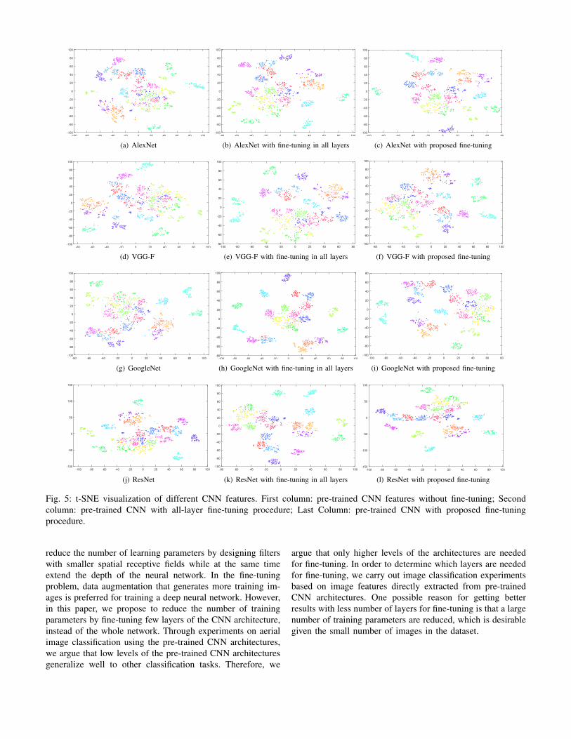
In order to qualitatively evaluate the performances of differ-ent features (pre-trained model, pre-trained model with fine-tuning on all layers, pre-trained model with proposed fine-tuning method), we adopt the t-Distributed Stochastic Neigh-bor Embedding (t-SNE) algorithm proposed in [18] to visual-ize the feature distributions for different classes. The algorithmperforms dimensionality reduction on high-dimensional dataand, at the same time, preserves the significant structures ofhigh-dimensional data. With all the CNN models available,we extract image features for the original image dataset with2100 images and apply t-SNE to reduce these image features

to two dimensions. The scatter plots of these images inthe corresponding reduced two-dimensional feature space areillustrated in Fig. 5. Each point in the plot represents an imagein the dataset and different classes are indicated with differentcolors. From these plots, it is obvious to see that image featuresextracted from the proposed fine-tuning method tend to clusterbetter in the reduced two dimensional feature space than thefeatures extracted using other two schemes, therefore it iseasier to differentiate them using a designed classifier.

The other way to compare the performances of differentCNN models is to visualize the filter weights and its corre-sponding activation outputs of various layers. We apply thetoolbox provided by Yosinski et al. [19] for this purpose. Inorder to demonstrate the idea, an “airplane” image from thedataset is fed into the modified pre-trained AlexNet model,the fine-tuned AlexNet model using the traditional fine-tunemethod, and the fine-tuned AlexNet model with the proposedapproach. For each layer of the network, the toolbox plotsthe learned weights and activation maps of the filters fromdifferent layers. Outputs from the low-level filters respondto edges and corners in the image while high-level filtersfrom CONV5 create meaningful objects. The last layer ofAlexNet contains 21 neurons, each one corresponds to theprobability of the image being classified as a spacific class.The “CONV5” response using the proposed fine-tuned modelis shown in Fig. 6. We also display the classification outputsfrom different CNN models in the same figure. Accordingto these results, only the model from our proposed fine-tuning scheme correctly classify the image as an airplane (withprobability of 0.88), while the other two methods classifythe image as “intersection” with probability of 0.5 and 0.41respectively, and consider it as an airplane with probability of0.3. To better understand what what filters in “CONV5” layerlearn from our dataset, we manually feed all the “airplane”image scenes from the UCMerced dataset [5] to the proposedfine-tuned AlexNet model and visualize the filter responsesfrom “CONV5” layer. We observe that one of the neuronsfrom “CONV5” layer obtains high response for image sceneswith single blue plane, as indicated in Fig. 7. These responsesalso indicate that the neuron is capable to detect planes withdifferent orientations.

V. DISCUSSION

One of the major difficulties regrading to training a deepneural network is to make sure that the trained neural networkis not over-fitted on the training dataset. As a result, the dropout (DROP) layer was proposed in AlexNet and VGG-F toreduce the number of training parameters when learning CNNarchitectures. On the other hand, the GoogleNet and ResNet

-100 -80 -60 -40 -20 0 20 40 60 80 100

-100

-80

-60

-40

-20

0

20

40

60

80

100

(a) AlexNet-80 -60 -40 -20 0 20 40 60 80 100

-100

-80

-60

-40

-20

0

20

40

60

80

100

(b) AlexNet with fine-tuning in all layers-100 -80 -60 -40 -20 0 20 40 60 80

-100

-80

-60

-40

-20

0

20

40

60

80

100

(c) AlexNet with proposed fine-tuning

-80 -60 -40 -20 0 20 40 60 80 100

-100

-80

-60

-40

-20

0

20

40

60

80

100

(d) VGG-F

-100 -80 -60 -40 -20 0 20 40 60 80

-80

-60

-40

-20

0

20

40

60

80

100

(e) VGG-F with fine-tuning in all layers

-80 -60 -40 -20 0 20 40 60 80 100

-100

-80

-60

-40

-20

0

20

40

60

80

100

(f) VGG-F with proposed fine-tuning

-80 -60 -40 -20 0 20 40 60 80 100

-100

-80

-60

-40

-20

0

20

40

60

80

100

(g) GoogleNet-100 -80 -60 -40 -20 0 20 40 60 80 100

-80

-60

-40

-20

0

20

40

60

80

100

(h) GoogleNet with fine-tuning in all layers

-100 -80 -60 -40 -20 0 20 40 60 80

-100

-80

-60

-40

-20

0

20

40

60

80

(i) GoogleNet with proposed fine-tuning

-100 -80 -60 -40 -20 0 20 40 60 80 100

-100

-50

0

50

100

150

(j) ResNet

-80 -60 -40 -20 0 20 40 60 80 100

-100

-80

-60

-40

-20

0

20

40

60

80

100

(k) ResNet with fine-tuning in all layers

-100 -80 -60 -40 -20 0 20 40 60 80 100

-150

-100

-50

0

50

100

(l) ResNet with proposed fine-tuning

Fig. 5: t-SNE visualization of different CNN features. First column: pre-trained CNN features without fine-tuning; Secondcolumn: pre-trained CNN with all-layer fine-tuning procedure; Last Column: pre-trained CNN with proposed fine-tuningprocedure.

reduce the number of learning parameters by designing filterswith smaller spatial receptive fields while at the same timeextend the depth of the neural network. In the fine-tuningproblem, data augmentation that generates more training im-ages is preferred for training a deep neural network. However,in this paper, we propose to reduce the number of trainingparameters by fine-tuning few layers of the CNN architecture,instead of the whole network. Through experiments on aerialimage classification using the pre-trained CNN architectures,we argue that low levels of the pre-trained CNN architecturesgeneralize well to other classification tasks. Therefore, we

argue that only higher levels of the architectures are neededfor fine-tuning. In order to determine which layers are neededfor fine-tuning, we carry out image classification experimentsbased on image features directly extracted from pre-trainedCNN architectures. One possible reason for getting betterresults with less number of layers for fine-tuning is that a largenumber of training parameters are reduced, which is desirablegiven the small number of images in the dataset.

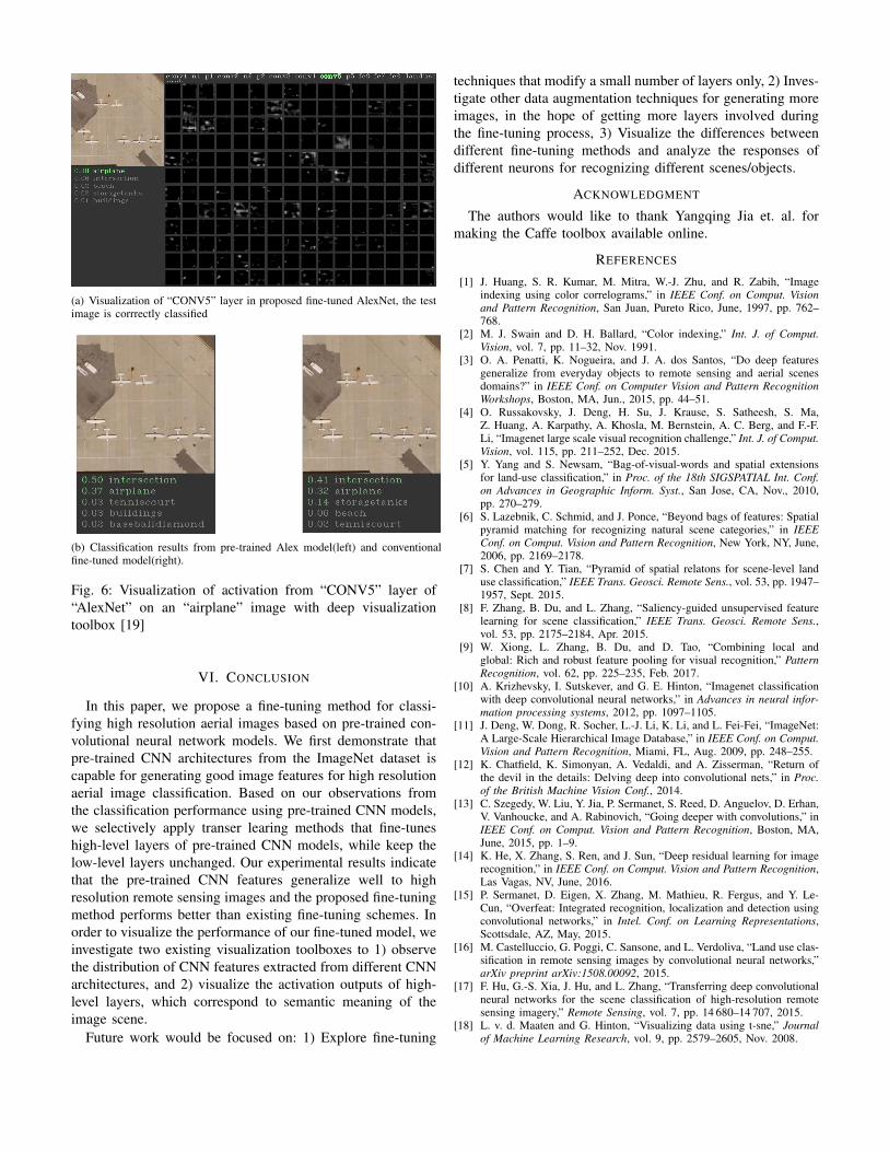
(a) Visualization of “CONV5” layer in proposed fine-tuned AlexNet, the testimage is corrrectly classified

(b) Classification results from pre-trained Alex model(left) and conventionalfine-tuned model(right).

Fig. 6: Visualization of activation from “CONV5” layer of“AlexNet” on an “airplane” image with deep visualizationtoolbox [19]

VI. CONCLUSION

In this paper, we propose a fine-tuning method for classi-fying high resolution aerial images based on pre-trained con-volutional neural network models. We first demonstrate thatpre-trained CNN architectures from the ImageNet dataset iscapable for generating good image features for high resolutionaerial image classification. Based on our observations fromthe classification performance using pre-trained CNN models,we selectively apply transer learing methods that fine-tuneshigh-level layers of pre-trained CNN models, while keep thelow-level layers unchanged. Our experimental results indicatethat the pre-trained CNN features generalize well to highresolution remote sensing images and the proposed fine-tuningmethod performs better than existing fine-tuning schemes. Inorder to visualize the performance of our fine-tuned model, weinvestigate two existing visualization toolboxes to 1) observethe distribution of CNN features extracted from different CNNarchitectures, and 2) visualize the activation outputs of high-level layers, which correspond to semantic meaning of theimage scene.

Future work would be focused on: 1) Explore fine-tuning

techniques that modify a small number of layers only, 2) Inves-tigate other data augmentation techniques for generating moreimages, in the hope of getting more layers involved duringthe fine-tuning process, 3) Visualize the differences betweendifferent fine-tuning methods and analyze the responses ofdifferent neurons for recognizing different scenes/objects.

ACKNOWLEDGMENT

The authors would like to thank Yangqing Jia et. al. formaking the Caffe toolbox available online.

REFERENCES

[1] J. Huang, S. R. Kumar, M. Mitra, W.-J. Zhu, and R. Zabih, “Imageindexing using color correlograms,” in IEEE Conf. on Comput. Visionand Pattern Recognition, San Juan, Pureto Rico, June, 1997, pp. 762–768.

[2] M. J. Swain and D. H. Ballard, “Color indexing,” Int. J. of Comput.Vision, vol. 7, pp. 11–32, Nov. 1991.

[3] O. A. Penatti, K. Nogueira, and J. A. dos Santos, “Do deep featuresgeneralize from everyday objects to remote sensing and aerial scenesdomains?” in IEEE Conf. on Computer Vision and Pattern RecognitionWorkshops, Boston, MA, Jun., 2015, pp. 44–51.

[4] O. Russakovsky, J. Deng, H. Su, J. Krause, S. Satheesh, S. Ma,Z. Huang, A. Karpathy, A. Khosla, M. Bernstein, A. C. Berg, and F.-F.Li, “Imagenet large scale visual recognition challenge,” Int. J. of Comput.Vision, vol. 115, pp. 211–252, Dec. 2015.

[5] Y. Yang and S. Newsam, “Bag-of-visual-words and spatial extensionsfor land-use classification,” in Proc. of the 18th SIGSPATIAL Int. Conf.on Advances in Geographic Inform. Syst., San Jose, CA, Nov., 2010,pp. 270–279.

[6] S. Lazebnik, C. Schmid, and J. Ponce, “Beyond bags of features: Spatialpyramid matching for recognizing natural scene categories,” in IEEEConf. on Comput. Vision and Pattern Recognition, New York, NY, June,2006, pp. 2169–2178.

[7] S. Chen and Y. Tian, “Pyramid of spatial relatons for scene-level landuse classification,” IEEE Trans. Geosci. Remote Sens., vol. 53, pp. 1947–1957, Sept. 2015.

[8] F. Zhang, B. Du, and L. Zhang, “Saliency-guided unsupervised featurelearning for scene classification,” IEEE Trans. Geosci. Remote Sens.,vol. 53, pp. 2175–2184, Apr. 2015.

[9] W. Xiong, L. Zhang, B. Du, and D. Tao, “Combining local andglobal: Rich and robust feature pooling for visual recognition,” PatternRecognition, vol. 62, pp. 225–235, Feb. 2017.

[10] A. Krizhevsky, I. Sutskever, and G. E. Hinton, “Imagenet classificationwith deep convolutional neural networks,” in Advances in neural infor-mation processing systems, 2012, pp. 1097–1105.

[11] J. Deng, W. Dong, R. Socher, L.-J. Li, K. Li, and L. Fei-Fei, “ImageNet:A Large-Scale Hierarchical Image Database,” in IEEE Conf. on Comput.Vision and Pattern Recognition, Miami, FL, Aug. 2009, pp. 248–255.

[12] K. Chatfield, K. Simonyan, A. Vedaldi, and A. Zisserman, “Return ofthe devil in the details: Delving deep into convolutional nets,” in Proc.of the British Machine Vision Conf., 2014.

[13] C. Szegedy, W. Liu, Y. Jia, P. Sermanet, S. Reed, D. Anguelov, D. Erhan,V. Vanhoucke, and A. Rabinovich, “Going deeper with convolutions,” inIEEE Conf. on Comput. Vision and Pattern Recognition, Boston, MA,June, 2015, pp. 1–9.

[14] K. He, X. Zhang, S. Ren, and J. Sun, “Deep residual learning for imagerecognition,” in IEEE Conf. on Comput. Vision and Pattern Recognition,Las Vagas, NV, June, 2016.

[15] P. Sermanet, D. Eigen, X. Zhang, M. Mathieu, R. Fergus, and Y. Le-Cun, “Overfeat: Integrated recognition, localization and detection usingconvolutional networks,” in Intel. Conf. on Learning Representations,Scottsdale, AZ, May, 2015.

[16] M. Castelluccio, G. Poggi, C. Sansone, and L. Verdoliva, “Land use clas-sification in remote sensing images by convolutional neural networks,”arXiv preprint arXiv:1508.00092, 2015.

[17] F. Hu, G.-S. Xia, J. Hu, and L. Zhang, “Transferring deep convolutionalneural networks for the scene classification of high-resolution remotesensing imagery,” Remote Sensing, vol. 7, pp. 14 680–14 707, 2015.

[18] L. v. d. Maaten and G. Hinton, “Visualizing data using t-sne,” Journalof Machine Learning Research, vol. 9, pp. 2579–2605, Nov. 2008.

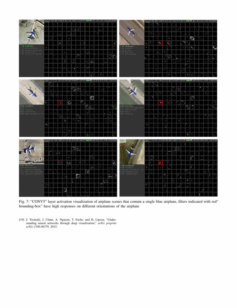
Fig. 7: “CONV5” layer activation visualization of airplane scenes that contain a single blue airplane, filters indicated with red“bounding-box” have high responses on different orientations of the airplane

[19] J. Yosinski, J. Clune, A. Nguyen, T. Fuchs, and H. Lipson, “Under-standing neural networks through deep visualization,” arXiv preprintarXiv:1506.06579, 2015.