Transcription Methods for Trajectory Optimization

A beginners tutorial

Matthew P. KellyCornell University

mpk72@cornell.edu

February 18, 2015

Abstract

This report is an introduction to transcription methods for trajectory optimization techniques. Thefirst few sections describe the two classes of transcription methods (shooting & simultaneous) that areused to convert the trajectory optimization problem into a general constrained optimization form. Themiddle of the report discusses a few extensions to the basic methods, including how to deal with hybridsystems (such as walking robots). The final section goes over a variety of implementation details.

1 Optimal Control Overview

There are three types of algorithms for solving optimal control problems[4]:

• Dynamic Programming: Solve Hamilton-Jacobi-Bellman Equations over the entire state space.

• Indirect Methods: Transcribe problem then find where the slope of the objective is zero.

• Direct Methods: Transcribe problem then find the minimum of the objective function.

Dynamic programming is an excellent solution to the optimal control problem for unconstrained low-dimensional systems, but it does not scale well to high-dimensional systems, since it requires a discretizationof the full state space. Indirect methods tend to be numerically unstable and are difficult to implement andinitialize [2]. For the remainder of this paper we will restrict focus to direct methods for transcribing andsolving the optimal control problem. The solution to an optimal control problem via transcription scaleswell to high-dimensional systems, but yields a single trajectory through state and control space, rather thana global policy like dynamic programming.

1.1 Trajectory Optimization Problem

A trajectory optimization problem seeks to find the a trajectory for some dynamical system that satisfiessome set of constraints while minimizing some cost functional. Below, I’ve laid out a general framework fora trajectory optimization problem.

Optimal Trajectory: {x∗(t),u∗(t)} (1)

System Dynamics: x = f(t,x,u) (2)

Constraints: cmin < c(t,x,u) < cmax (3)

Boundary Conditions: bmin < b(t0,x0, tf ,xf ) < bmax (4)

Cost Functional: J = φ(t0,x0, tf ,xf ) +

∫ tf

t0

g(t,x,u) dt (5)

One interesting thing to point out is the difference between a state x and a control u. A state variable is avariable that is differentiated in the dynamics equation, where as a control variable only appears algebraicallyin the dynamics equation [2]. In some cases there might also be unknown parameters (not shown) that aretime-invariant variables that appear algebraically in the dynamics equation.

1

arX

iv:1

707.

0028

4v1

[m

ath.

OC

] 2

Jul

201

7

1.2 Non-linear Programming

Transcription methods for solving an optimal control problem work by converting a continuous problem(Section 1.1) into a non-linear programming problem (7). Once in this form, the problem can be passed toa commercial solver, such as SNOPT[6], IPOPT[13], or FMINCON [8].

minimizez∈Rn

J(z) (6)

subject to: l ≤

zc(z)Az

≤ u (7)

There are many transcription algorithms that make this conversion, but they can all be divided up intotwo broad classes: shooting methods and simultaneous methods. The difference is based on how eachmethod enforces the constraint on the system’s dynamics. Shooting methods use a simulation to explicitlyenforce the system dynamics. Simultaneous methods enforce the dynamics at a series of points along thetrajectory.

2 Shooting Methods

Single-shooting is probably the simplest method for transcribing an optimal control problem. Consider theproblem of trying to hit a target with a cannon. You have two decision variables (firing angle and mass ofpowder) and one constraint (trajectory passes through target). The dynamics are simple (projectile motion)and the cost function is the mass of powder. The single shooting method is similar to what a person mightaccomplish with experiments. You make a guess at the angle and amount of powder, and then fire thecanon. If you shoot over the target, then perhaps you would reduce the mass of powder on the next test.By repeating this method, you would eventually be able to hit the target, while using as little powder aspossible. Single shooting works the same way, just replacing the experiments with simulations.

In a more general case of single shooting, with a continuous control input, you would choose somearbitrary function to approximate the input. A few common choices are zero-order-hold, piecewise linear,piecewise cubic, or orthogonal polynomials. If the control is modeled with a piecewise function, then youmust take care to align the discontinuities of the control with the integration steps in the simulation.

Single shooting works well enough for simple problems, but it will almost certainly fail on problems thatare more complicated. This is because the relationship between the decision variables and the objectiveand constraint functions is not well approximated by the linear (or quadratic) model that the non-linearprogramming solver uses.

Multiple shooting works by breaking up a trajectory into some number of segments, and using singleshooting to solve for each segment. As the segments get shorter, the relationship between the decisionvariables and the objective function and constraints becomes more linear. In multiple shooting, the end ofone segment will not necessarily match up with the start of the next. This difference is known as a defect,and it is added to the constraint vector. Adding all of the segments will increase the number of decisionvariables (the start of each segment) and the number of constraints (defects). Although it might seem thatthis would make the low-level optimization problem harder, it actually turns out to make it easier.

Figure 1 shows a cartoon comparing single shooting and multiple shooting.

3 Simultaneous Methods

There are a wide variety of simultaneous methods. The key difference between simultaneous methods andshooting methods is that simultaneous methods directly represent the state trajectory using decision vari-ables, and then satisfy the dynamics constraint only at special points in the trajectory.

2

Single ShootingC

ontr

ol

Time

Sta

te

Time

Arbitrary Function Approximator

Remove Defect

Simulation

Multiple Shooting

Contr

ol

Time

Sta

te

Time

Remove Defects

Simulation

Arbitrary Function Approximator

Knot Point

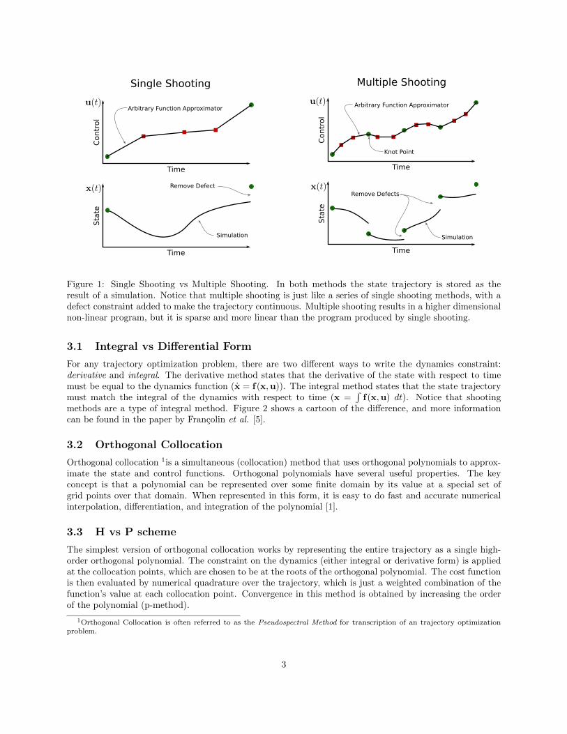
Figure 1: Single Shooting vs Multiple Shooting. In both methods the state trajectory is stored as theresult of a simulation. Notice that multiple shooting is just like a series of single shooting methods, with adefect constraint added to make the trajectory continuous. Multiple shooting results in a higher dimensionalnon-linear program, but it is sparse and more linear than the program produced by single shooting.

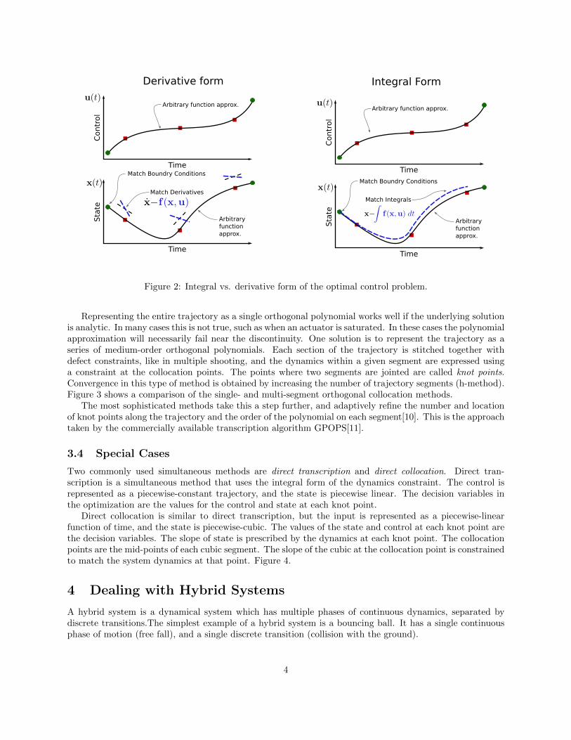
3.1 Integral vs Differential Form

For any trajectory optimization problem, there are two different ways to write the dynamics constraint:derivative and integral. The derivative method states that the derivative of the state with respect to timemust be equal to the dynamics function (x = f(x,u)). The integral method states that the state trajectorymust match the integral of the dynamics with respect to time (x =

∫f(x,u) dt). Notice that shooting

methods are a type of integral method. Figure 2 shows a cartoon of the difference, and more informationcan be found in the paper by Francolin et al. [5].

3.2 Orthogonal Collocation

Orthogonal collocation 1is a simultaneous (collocation) method that uses orthogonal polynomials to approx-imate the state and control functions. Orthogonal polynomials have several useful properties. The keyconcept is that a polynomial can be represented over some finite domain by its value at a special set ofgrid points over that domain. When represented in this form, it is easy to do fast and accurate numericalinterpolation, differentiation, and integration of the polynomial [1].

3.3 H vs P scheme

The simplest version of orthogonal collocation works by representing the entire trajectory as a single high-order orthogonal polynomial. The constraint on the dynamics (either integral or derivative form) is appliedat the collocation points, which are chosen to be at the roots of the orthogonal polynomial. The cost functionis then evaluated by numerical quadrature over the trajectory, which is just a weighted combination of thefunction’s value at each collocation point. Convergence in this method is obtained by increasing the orderof the polynomial (p-method).

1Orthogonal Collocation is often referred to as the Pseudospectral Method for transcription of an trajectory optimizationproblem.

3

Integral FormC

ontr

ol

Time

Sta

te

Time

Arbitrary function approx.

Match Derivatives

Derivative form

Contr

ol

Time

Sta

te

Time

Match Integrals

Arbitraryfunctionapprox.

Arbitrary function approx.

Arbitraryfunctionapprox.

Match Boundry ConditionsMatch Boundry Conditions

Figure 2: Integral vs. derivative form of the optimal control problem.

Representing the entire trajectory as a single orthogonal polynomial works well if the underlying solutionis analytic. In many cases this is not true, such as when an actuator is saturated. In these cases the polynomialapproximation will necessarily fail near the discontinuity. One solution is to represent the trajectory as aseries of medium-order orthogonal polynomials. Each section of the trajectory is stitched together withdefect constraints, like in multiple shooting, and the dynamics within a given segment are expressed usinga constraint at the collocation points. The points where two segments are jointed are called knot points.Convergence in this type of method is obtained by increasing the number of trajectory segments (h-method).Figure 3 shows a comparison of the single- and multi-segment orthogonal collocation methods.

The most sophisticated methods take this a step further, and adaptively refine the number and locationof knot points along the trajectory and the order of the polynomial on each segment[10]. This is the approachtaken by the commercially available transcription algorithm GPOPS[11].

3.4 Special Cases

Two commonly used simultaneous methods are direct transcription and direct collocation. Direct tran-scription is a simultaneous method that uses the integral form of the dynamics constraint. The control isrepresented as a piecewise-constant trajectory, and the state is piecewise linear. The decision variables inthe optimization are the values for the control and state at each knot point.

Direct collocation is similar to direct transcription, but the input is represented as a piecewise-linearfunction of time, and the state is piecewise-cubic. The values of the state and control at each knot point arethe decision variables. The slope of state is prescribed by the dynamics at each knot point. The collocationpoints are the mid-points of each cubic segment. The slope of the cubic at the collocation point is constrainedto match the system dynamics at that point. Figure 4.

4 Dealing with Hybrid Systems

A hybrid system is a dynamical system which has multiple phases of continuous dynamics, separated bydiscrete transitions.The simplest example of a hybrid system is a bouncing ball. It has a single continuousphase of motion (free fall), and a single discrete transition (collision with the ground).

4

Single-Segment Pseudospectral

Contr

ol

Time

Sta

te

Time

High-OrderOrthogonalPolynomial

OrthogonalPolynomial

Roots of Orthogonal Polynomial(Quadrature / Collocation Points)

Multi-Segment Pseudospectral

Contr

ol

Time

Sta

te

Time

Piecewise Medium-OrderOrthogonal Polynomial

Knot Point

Piecewise Medium-OrderOrthogonal Polynomial

Quadrature Point

"p" Method; Convergence by increasing polynomial order "h" Method; Convergence by increasing number of segments

Figure 3: Orthogonal Collocation Methods

Direct Transcription

Contr

ol

Time

Sta

te

Time

Remove Defects

Euler Integration

Fine Grid

Zero-Order-Hold

Direct Collocation

Contr

ol

Time

Sta

te

Time

Piecewise CubicHermite Polynomial

Knot Point

Piecewise Linear

KnotPoint

Match Slopesat Collocation-Points

Figure 4: Special Cases of simultaneous methods

5

A more complicated hybrid system would be a walking robot. A few examples of continuous modes mightbe:

• flight - both feet in the air• double stance - both feet on the ground• single stance - one foot on the ground

There would then be a discrete transition between each of these modes. Some transitions do not alter thecontinuous state (such as lifting a foot off of the ground), while other transitions do change the continuousstate (a foot colliding with the ground).

A naive way to handle such hybrid systems would be to bundle them up inside a big simulation ordynamics function and try to just make a simple transcription method work. This will almost certainlyfail. The reason is that the underlying optimization algorithm is typically a smooth, gradient-based method(eg. SNOPT, IPOPT, FMINCON). The discrete transitions of the hybrid system cause the dynamics to benon-smooth. For example, a small change in one variable could cause the collision to happen at a differenttime, which would then cause a huge change in the defect constraints.

There are two generally accepted methods for dealing with hybrid systems: multi-phase methods, andthrough-contact methods. Multi-phase methods are faster and more accurate, but they require explicitknowledge of the sequence of transitions. Through-contact methods can deal with arbitrary sequences ofcontacts, but are slower and less accurate.

These two methods are analogous to the two different methods of simulation hybrid systems. Multi-phasetranscription is like simulating a finite state machine using event detection. Through-contact is analogousto time-stepping.

4.1 Multi-Phase Methods

Multi-phase methods are a fairly simple extension of the basic multiple shooting or collocation algorithms.First, the user decides which sequence of phases should occur. For example, in a walking robot, this mightbe single stance (one foot on the ground) followed by double stance (two feet on the ground). Then theconstraints are set up within each of those continuous phases exactly the same as in a simpler problem. Thena set of constraints are added to switch the continuous phases together, satisfying the transition equations.

One interesting side effect of this method is that the state of the system can be completely different ineach phase of motion, provided that there is some sensible way to link them. This is useful, because it meansthat each set of continuous dynamics can be written in minimal coordinates.

The commercially available transcription program GPOPS II [11] provides a sophisticated interface forsetting up and solving hybrid system trajectories using multi-phase methods.

4.2 Through-Contact Methods

Through-contact methods take a completely different approach. Instead of pushing the discontinuities in thedynamics to a special constraints between each phase, they directly handle the contact constraints at everygrid point.

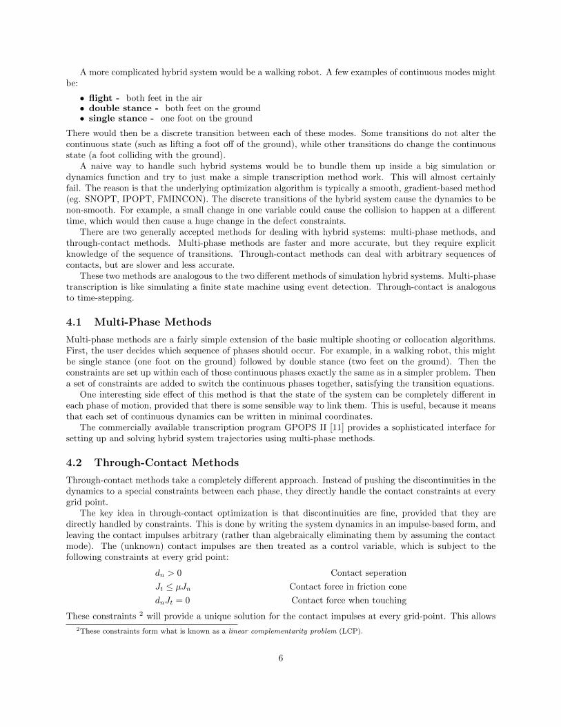
The key idea in through-contact optimization is that discontinuities are fine, provided that they aredirectly handled by constraints. This is done by writing the system dynamics in an impulse-based form, andleaving the contact impulses arbitrary (rather than algebraically eliminating them by assuming the contactmode). The (unknown) contact impulses are then treated as a control variable, which is subject to thefollowing constraints at every grid point:

dn > 0 Contact seperation

Jt ≤ µJn Contact force in friction cone

dnJt = 0 Contact force when touching

These constraints 2 will provide a unique solution for the contact impulses at every grid-point. This allows

2These constraints form what is known as a linear complementarity problem (LCP).

6

for an arbitrary sequence of contacts throughout the trajectory, which is particularly useful for complexbehaviors, such as a biped crawling, or standing up from a laying down position, as shown by Mordatch etal [9].

Through-contact trajectory optimization will soon be included as part of Drake [12], a toolbox for doingrobot control design and analysis.

4.3 Accuracy of each method

If the sequence of contact modes is unknown, then a through contact method might be more accurate becauseit can find solution that would be excluded by the prescribed sequence of phases in the multi-phase method.That being said, if both methods manage to find roughly the same solution, then the multi-phase methodwill be far more accurate.

The multi-phase method can be incredibly accurate because the optimization is implicitly doing rootfinding for the transitions between each continuous phase of motion. In addition to that, the continuoustrajectory can be easily represented by a high-order polynomial (either directly in collocation, or indirectlythrough a Runge-Kutta scheme in multiple shooting). These high-order trajectories are able to match thetrue solution very well, even with relatively large time steps, since the errors are proportional to the orderof the polynomial.

The through-contact methods are inherently limited in their accuracy because the transitions betweencontinuous phases of motion are constrained to grid-points, which are not able to be independently adjusted.This means that the approximation errors are proportional to the step-size, drastically limiting the abilityto get high-accuracy solutions.

5 Setting up your problem

5.1 Grid Selection

Both shooting and simultaneous methods have some free parameter(s) that control the grid that it is usedto transcribe the problem. In general, you need a fine grid for an accurate solution, but this can causeconvergence problems if the initial guess is not very good. A common solution is to use a very coarse grid tofind an approximate solution, and then use this approximate solution as an initial guess for a second, or third,optimization using a finer grid. The commercially available program GPOPS II handles this grid-refinementautomatically using a sophisticated algorithm [3].

5.2 Initialization

Even a well-posed trajectory optimization is likely to fail with a poor initialization. One good method forinitializing a trajectory is to guess a few points on the trajectory, and then fit a polynomial to these points.Then this polynomial can be differentiated once to get the first derivatives of the state, and again to get thejoint accelerations. Inverse dynamics can then be used to compute the joint torques necessary to producethose accelerations. Then interpolate this rough guess to get the correct grid-points for either your multipleshooting or collocation method.

One thing that can go wrong with initialization is that you start the optimization with an infeasible, butlocally optimal solution. This commonly occurs when you set the initial control functional to zero. Thiscan be corrected by added a small random noise along the initial guess at the actuator. This has the addedbenefit of starting you optimization from a new place on each iteration, which can sometimes be helpful todetect local minima.

Sometimes the optimization will fail, even with a reasonable initialization, if the cost function is toocomplicated3. One solution is to write the optimization to use an alternate cost function, such as torque-

3Cost of transport, which is total energy used by a robot divided by it’s weight multiplied by the distance travelled, is aparticularly difficult cost function to optimize.

7

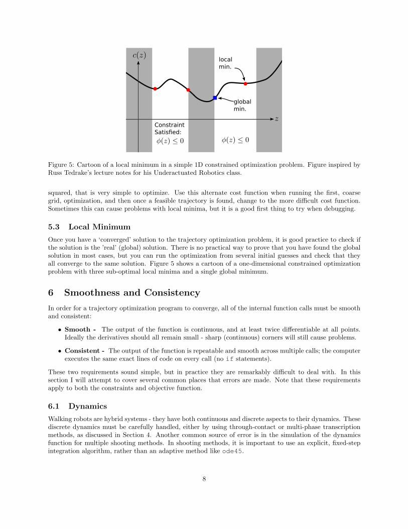
ConstraintSatisfied:

globalmin.

localmin.

Figure 5: Cartoon of a local minimum in a simple 1D constrained optimization problem. Figure inspired byRuss Tedrake’s lecture notes for his Underactuated Robotics class.

squared, that is very simple to optimize. Use this alternate cost function when running the first, coarsegrid, optimization, and then once a feasible trajectory is found, change to the more difficult cost function.Sometimes this can cause problems with local minima, but it is a good first thing to try when debugging.

5.3 Local Minimum

Once you have a ‘converged’ solution to the trajectory optimization problem, it is good practice to check ifthe solution is the ’real’ (global) solution. There is no practical way to prove that you have found the globalsolution in most cases, but you can run the optimization from several initial guesses and check that theyall converge to the same solution. Figure 5 shows a cartoon of a one-dimensional constrained optimizationproblem with three sub-optimal local minima and a single global minimum.

6 Smoothness and Consistency

In order for a trajectory optimization program to converge, all of the internal function calls must be smoothand consistent:

• Smooth - The output of the function is continuous, and at least twice differentiable at all points.Ideally the derivatives should all remain small - sharp (continuous) corners will still cause problems.

• Consistent - The output of the function is repeatable and smooth across multiple calls; the computerexecutes the same exact lines of code on every call (no if statements).

These two requirements sound simple, but in practice they are remarkably difficult to deal with. In thissection I will attempt to cover several common places that errors are made. Note that these requirementsapply to both the constraints and objective function.

6.1 Dynamics

Walking robots are hybrid systems - they have both continuous and discrete aspects to their dynamics. Thesediscrete dynamics must be carefully handled, either by using through-contact or multi-phase transcriptionmethods, as discussed in Section 4. Another common source of error is in the simulation of the dynamicsfunction for multiple shooting methods. In shooting methods, it is important to use an explicit, fixed-stepintegration algorithm, rather than an adaptive method like ode45.

8

Sometimes it might be tempting to put some sort of noise into the dynamics. This guarantees that thefunction will be inconsistent, and will almost certainly cause the optimization program to fail. In general,there is no good reason to put a call to a random number generator inside of a trajectory optimizationprogram.

6.2 Objective Function

There are many sources of discontinuity inside of an objective function, typically due to seeming innocuousfunctions. A few examples are taking the maximum or minimum of a list of numbers, the absolute valuefunction, clamp function4, and the ramp function.

The best way to deal with these discontinuous functions is by using a constraint to enforce the discontinu-ity. This works because the non-linear program solver has special tools build-in for dealing with constraints.Equation 8 shows the correct way to handle the function |x|. Other examples are provided in [7].

|x| = x1 + x2 subject to

x = x1 − x2x1 >= 0

x2 >= 0

(8)

Another approach to dealing with discontinuous functions is to use ‘smooth’ approximations, as shownbelow:

|x| ≈ x tanh (x/α)

max(x) ≈ α log(∑

expx

α

)This method works, but it will typically be less accurate and take longer to converge than the constraint

method. Even though the smoothed functions are continuous, there is a tradeoff between accuracy andconvergence. If the smoothing is large, then the optimization program will converge, but with an inaccuratesolution. If the smoothing is small, the program will converge slowly, or perhaps not at all. One solutionis to iteratively reduce the smoothing, starting with heavy smoothing to get a feasible solution, and thenreducing the smoothing to zero in on the answer.

There are two approaches to making smooth approximations of functions. The first is to use exponentialfunctions that asymptotically approach the true function far from the discontinuity. The second is to usea piecewise version of the function, where the region near the discontinuity is replaced with a polynomialapproximation.

7 Software Specifics

Once a trajectory optimization problem been transcribed by either multiple shooting or collocation, it mustthen be solved by nonlinear constrained optimization solver. Two of the most popular algorithms are SNOPTand FMINCON. The following section describe some specific details that are helpful when working with eachof these programs.

It seems that FMINCON solves the multiple shooting problem by first finding a feasible solution, andthen attempting to optimize it. This means that FMINCON can handle a worse initial guess than SNOPT,but it is a little worse at finding the true optimal solution, because it does not allow for much flexibility inthe constraints.

Instead of writing your own transcription algorithm, it is possible to buy a commercial version. Thebest available software now is probably GPOPS II, which internally calls either SNOPT or IPOPT (anothersolver, not discussed here).

4Also called saturation

9

7.1 SNOPT [6]

A single function call is used for the objective function and all constraints. This function returns a vector,and the first element of the vector is the value of the objective function. All of the following elementsare constraints. SNOPT does not require the user to specify which constraints are linear or nonlinear - itautomatically computes this.

Since SNOPT combines the objective function and the constraint function, you always need to providea value for the objective function, even if you are only solving a feasibility problem. In this case, the valueof the objective function should be set to zero. More importantly, you must also specify that the bounds ofthe objective function are also zero. In code this looks like:F(1)==0, Flow(1)==0, Fupp(1)==0

Do not use a constant term anywhere in your objective function or constraints. All constant terms mustbe moved to the boundary vectors (Flow, Fupp). This is because of how SNOPT internally stores andestimates the gradients - it will numerically remove any constant terms.

SNOPT does not allow the user to pass any parameters to the objective function, at least when calledfrom Matlab. One way to get around this is to create a single struct of parameters, and save it as a globalvariable. Once this is done, you can then just read the parameters off the global variable.

7.2 FMINCON [8]

FMINCON requires that the objective function and constraint function are in separate functions. Thiscreates a problem, because both the constraints and objective need to evaluate the dynamics at every grid-point. To avoid doing all of the work twice, it is best to use a persistent variable (this would be a staticvariable in C++). Create a single function that does the integration of the dynamics, and have it store thelast input state and output solution. When it is called, it checks if the state is the same as last time - if itis, then just return the previous solution.

There is a bug of sorts in FMINCON, which prevents you from using state bounds to constrain a stateto a specific value. Basically, saying: 0 < x <= 0 causes FMINCON to try to divide by a step size ofmachine precision when doing its finite differencing. Much better to place these sorts of things as an equalityconstraint, which are handled in a special way.

7.3 GPOPS2 [11]

GPOPS2 is a commercially available software which implements “a general-pupose software for solving op-timal control problems using variable-order adaptive orthogonal collocation methods together with sparsenonlinear programming” This program is excellent at solving trajectory optimization problems which havea known sequence of contact modes, making an extremely general solver. In my experience it is generallymuch faster and more accurate than using a more simple multiple shooting or collocation method.

8 Miscellaneous

This section covers a few odd topics that are useful to understand, but do not fit elsewhere.

8.1 Regularization

It is possible to create an optimal trajectory problem which does not have a unique solution. This willgenerally cause convergence problems, as the optimization program bounces between seemingly equivalentsolutions. This problem is solved by adding a small regularization term to the objective function, whichforces a unique solution. For dynamical systems, I have found that adding a small input-squared term to thecost function is generally sufficient. I’ve found regularization terms that are 6-8 orders of magnitude smallerthan the primary objective term are often still effective.

10

8.2 Constraint on Controls

The correct way to apply a non-linear constraint to a control at the boundary of a trajectory is to createa dummy state to represent the control, and then let the optimization program determine the derivative ofthe control. The system dynamics can then be used to ensure feasibility of the control and its derivative.This technique is particularly useful for enforcing that the contact forces of a walking robot stay within theirfriction cone.

8.3 Optimizing a Parameter

Suppose that you would like to find an optimal trajectory, but there is at least one free parameter for yourdesign. It is tempting to just add this parameter as an additional term when passed to the underlyingoptimization function. This is a bad idea, because it couples the Jacobian of the constraints, which is almostas bad as solving the problem using single shooting. The correct thing to do is to add a control to thesystem, and use the control instead of the parameter. A special constraint is then added to ensure that thecontrol remains constant throughout the trajectory. This will quickly solve for the best possible parameterchoice, while keeping the Jacobian of the constraints and objective function sparse.

9 Hammer Example

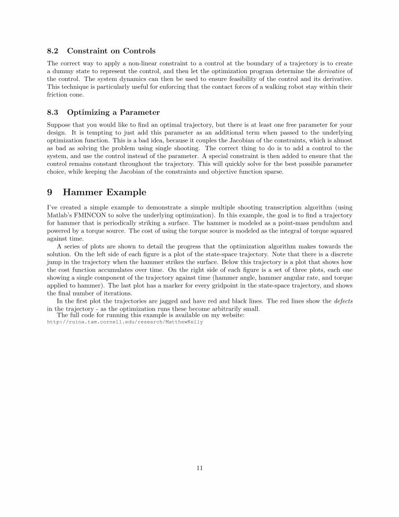
I’ve created a simple example to demonstrate a simple multiple shooting transcription algorithm (usingMatlab’s FMINCON to solve the underlying optimization). In this example, the goal is to find a trajectoryfor hammer that is periodically striking a surface. The hammer is modeled as a point-mass pendulum andpowered by a torque source. The cost of using the torque source is modeled as the integral of torque squaredagainst time.

A series of plots are shown to detail the progress that the optimization algorithm makes towards thesolution. On the left side of each figure is a plot of the state-space trajectory. Note that there is a discretejump in the trajectory when the hammer strikes the surface. Below this trajectory is a plot that shows howthe cost function accumulates over time. On the right side of each figure is a set of three plots, each oneshowing a single component of the trajectory against time (hammer angle, hammer angular rate, and torqueapplied to hammer). The last plot has a marker for every gridpoint in the state-space trajectory, and showsthe final number of iterations.

In the first plot the trajectories are jagged and have red and black lines. The red lines show the defectsin the trajectory - as the optimization runs these become arbitrarily small.

The full code for running this example is available on my website:http://ruina.tam.cornell.edu/research/MatthewKelly

11

0 0.5 1 1.5 2 2.5−10

−5

0

5

10

15

Angle (rad)

Rat

e (r

ad/s

)

Iteration: 1

0 0.1 0.2 0.3 0.4 0.5 0.6 0.7 0.8 0.9 10

2

4

6

8x 10

−18

Time (s)

Cos

t

0 0.1 0.2 0.3 0.4 0.5 0.6 0.7 0.8 0.9 1−10

−5

0

5

10

15

Time (s)

Ang

le (

rad)

Total Cost: 7.791e−18

0 0.1 0.2 0.3 0.4 0.5 0.6 0.7 0.8 0.9 10

0.5

1

1.5

2

2.5

Time (s)

Rat

e (r

ad/s

)

0 0.1 0.2 0.3 0.4 0.5 0.6 0.7 0.8 0.9 10

0.5

1

1.5

2x 10

−8

Time (s)

Tor

que

(Nm

)

Figure 6: The first iteration of the optimization program. Notice that FMINCON has added a smallperturbation to the guess at the control, to help numerically calculate the Jacobian. The initial guess was atrajectory made of two straight lines, and the initial defects are clearly visible.

−0.4 −0.2 0 0.2 0.4 0.6 0.8 1 1.2 1.4 1.6−10

−5

0

5

10

15

Angle (rad)

Rat

e (r

ad/s

)

Iteration: 3

0 0.1 0.2 0.3 0.4 0.5 0.6 0.7 0.8 0.90

0.05

0.1

0.15

0.2

Time (s)

Cos

t

0 0.1 0.2 0.3 0.4 0.5 0.6 0.7 0.8 0.9−10

−5

0

5

10

15

Time (s)

Ang

le (

rad)

Total Cost: 0.1839

0 0.1 0.2 0.3 0.4 0.5 0.6 0.7 0.8 0.9−0.5

0

0.5

1

1.5

2

Time (s)

Rat

e (r

ad/s

)

0 0.1 0.2 0.3 0.4 0.5 0.6 0.7 0.8 0.9−1

−0.5

0

0.5

1

Time (s)

Tor

que

(Nm

)

Figure 7: Even after a few iterations, the defects are no longer visible on the plot - the trajectory is nearlyfeasible . Notice that the optimization has a first guess at the actuation, and a non-zero cost function.

12

−0.2 0 0.2 0.4 0.6 0.8 1 1.2 1.4 1.6−6

−4

−2

0

2

4

6

8

10

12

14

Angle (rad)

Rat

e (r

ad/s

)

Iteration: 8

0 0.1 0.2 0.3 0.4 0.5 0.6 0.7 0.8 0.90

0.05

0.1

0.15

0.2

Time (s)

Cos

t

0 0.1 0.2 0.3 0.4 0.5 0.6 0.7 0.8 0.9−10

−5

0

5

10

15

Time (s)

Ang

le (

rad)

Total Cost: 0.12432

0 0.1 0.2 0.3 0.4 0.5 0.6 0.7 0.8 0.9−0.5

0

0.5

1

1.5

2

Time (s)

Rat

e (r

ad/s

)

0 0.1 0.2 0.3 0.4 0.5 0.6 0.7 0.8 0.9−1

−0.5

0

0.5

1

Time (s)

Tor

que

(Nm

)

Figure 8: Now the trajectory has roughly stabilized, and the optimization program is trying to make smallchanges to the control to reduce the total cost of the trajectory. Interestingly, the trajectory is smooth, butthe control is still fairly discontinuous. This is indicative of an solution that has not fully converged.

0 0.2 0.4 0.6 0.8 1 1.2 1.4 1.6−4

−2

0

2

4

6

8

10

12

14

Angle (rad)

Rat

e (r

ad/s

)

Iteration: 148

0 0.2 0.4 0.6 0.8 1 1.2 1.40

0.02

0.04

0.06

0.08

0.1

Time (s)

Cos

t

0 0.2 0.4 0.6 0.8 1 1.2 1.40

0.5

1

1.5

2

Time (s)

Ang

le (

rad)

Total Cost: 0.087013

0 0.2 0.4 0.6 0.8 1 1.2 1.4−5

0

5

10

15

Time (s)

Rat

e (r

ad/s

)

0 0.2 0.4 0.6 0.8 1 1.2 1.4−1

−0.5

0

0.5

1

Time (s)

Tor

que

(Nm

)

Figure 9: After 148 iterations the optimization program terminated. Notice that all components of thetrajectory are smooth, including the control function. I’ve put small circles over the start and end of eachsegment of the trajectory, which now line up almost perfectly.

13

References[1] Jean-Paul Berrut and Lloyd N. Trefethen. Barycentric Lagrange Interpolation *. 46(3):501–517, 2004.

[2] John T. Betts. Practical Methods for Optimal Control and Estimation Using Nonlinear Programming. Siam, 2010.

[3] Christopher L Darby, William W Hager, and Anil V Rao. An hp -adaptive pseudospectral method for solving optimalcontrol problems. (August 2010):476–502, 2011.

[4] Moritz Diehl, Hans Georg Bock, Holger Diedam, Pierre-brice Wieber, Pierre-brice Wieber Fast, and Direct Multiple. FastDirect Multiple Shooting Algorithms for Optimal Robot. In Fast Direct Multiple Shooting Algorithms for Optimal RobotControl, Heidelberg, Germany, 2004.

[5] Camila C Francolin, David A Benson, William W Hager, and Anil V Rao. Costate Estimation in Optimal Control UsingIntegral Gaussian Quadrature Orthogonal Collocation Methods. Optimal Control Applications and Methods, 2014.

[6] Philip E Gill, Walter Murray, and Michael A Saunders. SNOPT : An SQP Algorithm for Large-Scale Constrained. 47(1),2005.

[7] John T. Betts. Practical Methods for Optimal Control Using Nonlinear Programming. 2001.

[8] Mathworks. Matlab Optimization Toolbox, 2014.

[9] Igor Mordatch, Emanuel Todorov, and Zoran Popovic. Discovery of complex behaviors through contact-invariant opti-mization. ACM Transactions on Graphics, 31(4):1–8, July 2012.

[10] Michael A Patterson, William W Hager, and Anil V Rao. A ph Collocation Scheme for Optimal Control. pages 1–40.

[11] Michael A Patterson and Anil V Rao. GPOPS II : A MATLAB Software for Solving Multiple-Phase Optimal ControlProblems Using hp Adaptive Gaussian Quadrature Collocation Methods and Sparse Nonlinear Programming. 39(3):1–41,2013.

[12] Russ Tedrake. Drake – A planning, control, and analysis toolbox for nonlinear dynamical systems. Technical report, 2014.

[13] a Wachter and L T Biegler. On the implementation of primal-dual interior point filter line search algorithm for large-scalenonlinear programming, volume 106. 2006.

14