Embed Size (px)
Citation preview

TRANSACTIONS OF SOCIETY OF ACTUARIES 1995 VOL. 47
ACTUARIAL USAGE OF GROUPED DATA: AN APPROACH TO INCORPORATING SECONDARY DATA
PATRICK L. BROCKETF,* SAMUEL H. COX, BOAZ C~LANY, t FRED Y. PHILLIPS,, AND YUN SONG§
ABSTRACT
This paper addresses some pervasive problems in using secondary data in actuarial research, These problems include: • Reconciling and matching information from two or more sources • Estimating the probability and other statistics using banded data • Reconstructing the distribution function from summarized secondary
data • Incorporating information into derivation of life or loss distributions. An approach to solving these problems is based on information theory. Ex- plicit mathematical formulas for the probability distributions under study are presented in several specific settings with incomplete or grouped data and concomitant auxiliary information.
1. INTRODUCTION
This paper addresses certain pervasive problems in using secondary data in actuarial research. Those problems include the following situations: • The data are summarized in a histogram or tabular (grouped data) format,
perhaps with additional mean or median information (for example, pub- lished medical research, demographic data, and so on), which must be incorporated into actuarial analysis.
• Two published sources yield histogram or tabular summaries with the same variable, but the two sources do not group the values of the variable
*Dr. Brockett, not a member of the Society, is Director of the Center for Cybernetic Studies at the University of Texas at Austin.
"['Dr. Golany, not a member of the Society, is Associate Professor and Associate Dean, Faculty of Industrial Engineering and Management at the Technion-lsrael Institute of Technology, Technion City, Haifa, Israel.
:[:Dr, Phillips, not a member of the Society, is Director, Business School, Oregon Graduate In- stitute of Science and Technology, Portland, Oregon.
§Dr, Song, not a member of the Society, is on the actuarial staff of the National Actuarial Services Group, Ernst & Young, LLP, New York City.
89

90 TRANSACTIONS, VOLUME XLVII
the same way (for example, mortality rates grouped into age intervals can be distinctly different in different medical studies).
• The researcher wishes to answer a question by using information from several distinctly grouped data streams, and the original, detailed data underlying the published summary (which might give a better answer to the question) are unavailable.
Reconciling and matching information from two or more sources is a common analytic problem faced by practicing actuaries. Data reported by magazines, medical journals, or government publications are often given in grouped histogram form. Because these information sources operate inde- pendently of one another, their reports usually have incompatibly grouped data. The summary presentation of such information frequently is accom- panied by values of some of its moments or the conditional moments with certain subintervals. This data-matching problem is a specific case of the more general question, "How can we make statistical inferences from sec- ondary data and incorporate this information into our actuarial analysis?" In this paper we present a method (a maximum-entropy procedure) that is based on the concepts of statistical information theory and that shows how to use all the information available (and no other) to answer such questions.
Applications with real data often involve conflicting or missing data ele- ments. A publication may provide a histogram along with its overall mean and one conditional mean (that is, the mean of some subinterval), in which the latter two do not agree because of typographical error or because they are a summarization of two different studies.
Situations can also arise in which the data given are insufficient even to apply information theoretic techniques, but a uniform treatment is s011 needed. Accordingly, the rigorous statistical procedures detailed in Brockett [3] must be supplemented with some heuristics to handle these cases. These heuristic procedures also are discussed.
In this paper we present a procedure for generating maximum-entropy density estimates from data in histogram form with the possibility that ad- ditional means and medians may be known. With the computing power now available, completely rigorous maximum-entropy estimates can be obtained for nearly any consistent "information scenario" (combinations of infor- mation about moments and conditional moments of the density function that are consistent with at least one probability distribution). This paper provides illustrations of this.
While in general the histograms analyzed are analogous to probability densities, the procedure can also be used in some cases for more general

ACTUARIAL USAGE OF GROUPED DATA 91
"y=f(x)" variate relationships, where y is a continuous function of x. Grad- uation of mortality rates by information theoretic methods provides an ex- ample (compare Brockett and Zhang [10] and Brockett, Li, et al. [8]). Other applications are risk analysis and individual risk profile analysis.
2. DEFINITION
The early literature on statistical information theory was developed by Kullback and Leihler [16] following the work of Khinchine [14] and grew out of the engineering literature on communication theory. A complete in- troduction and description as well as applications of information theory to problems in actuarial science can be found in Brockett [3]. To summarize, in information theoretic notation, the expected information for distinguishing between two measures, p and q, is denoted by l(plq)- This expected infor- mation is mathematically quantified by the expected log-odds ratio; that is,
where p and q are discrete with masses Pi and qi for each i. Extensive discussion of the information functional (2.1) and its role as a unifying concept for statistics can be extracted from Kullback [15]. Brockett [3] also places the functional in perspective for actuarial science.
By applying Jensen's inequality to the function h(x)=x-lnx, l(plq)-->0 with l(plq)=0 if and only if p=q . As a consequence, the quantity l(plq) can be thought of as the (pseudo-) distance or "closeness measure" between p and q within the space of all measures having equal total mass. In our case, we want to choose that measure p that is "as close as possible" to some given measure q and that satisfies certain additional knowledge we have about p. The measure q is the benchmark, or beginning measure, and p is the measure we want to obtain. The additional information about p is written in the form of constraints that p must satisfy. Accordingly, our prob- lem becomes one of minimizing l(plq) over all possible p, subject to the given constraints on p. The solution p* to minimizing (2. l) subject to con- straints is referred to as the minimum discrimination information (MDI) estimate.
In many applications, however, there is no such a priori, benchmark, or starting-point measure q from which to derive p. In this case, we express our ignorance about q by choosing all values of q to be equally likely; that

92 TRANSACTIONS, VOLUME XLVII
is, q,.= 1 for all i in the discrete measure case or q (x )= l for all x in the continuous density case. Accordingly, our objective function (in the discrete case) is of form
Mi.,+,+
or equivalently
(2.2)
The quantity X i Pi ln(pi) is called the entropy of p, and the distribution that solves (2.2) is called the maximum-entropy (ME) distribution. The en- tropy of a distribution conceptually measures the dispersion of the distri- bution: the maximum-entropy distribution is the uniform distribution (most uniformly dispersed distribution) and the maximum entropy distribution is a point mass distribution with all its mass at a single point (the most con- centrated distribution possible).
The principles used in this paper are set forth by Kullback [15], Theil and Feibig [20], Brockett [3], and Brockett, Charnes, et al. [4]. What follows most closely resembles the latter two works, in that inferences are based on data that have already been summarized, rather than on original sample observations. The heuristic that connects with the maximum-entropy choice of probability distribution is that, all the information that is known about the unknown distribution p is written down. This information constitutes the constraint set that p must satisfy. The uncertainty (entropy) of p is then maximized subject to these constraints. In essence, what is known is used, and the uncertainty of what is not known is maximized.
3. SOME MOTIVATING EXAMPLES
To illustrate the problems discussed in Section 1, we examine the medical study by DeVivo et al. [11] on the mortality effects of incomplete and com- plete paraplegia and quadriplegia resulting in the relative mortality ratio data extracted in Table 1. The age intervals used in the medical study were de- fined as: 1-24, 25-49, and 50+, and the published reports are based on these intervals.

ACTUARIAL USAGE OF GROUPED DATA
TABLE 1
RELATIVE MORTALITY RATIOS FOR 5,131 SPINAL CORD INJURY PATENTS
INJURED BETWEEN 1973 AND 1980 WHO SURVIVED AT LEAST 24 HOURS
AFTER INJURY; BY NEUROLOGICAL CATEGORY AND AGE GROUP AT TIME OF INJURY [l !]
Neurological Category Relative and Age Group at Injury Mortality Ratio
Incomplete Paraplegia 1-24 25--49 50+
Complete Paraplegia 1-24 25--49 50+
Incomplete Quadriplegia 1-24 25--49 50+
Complete Quadriplegia 1-24 25-49 50+
4.82 6.59 3.26
4.93 6.93 3.26
4.22 6.71 3.95
12.4 20.78 14.11
93
An actuary might attempt to use these data for adjusting a mortality table for use in such cases as wrongful injury damage award compensation cal- culations and life insurance premium determination for medically impaired lives. A reasonable question is: Is there a statistically rigorous way to esti- mate, consistent with the data given in Table 1, the mortality rates for, say, incomplete paraplegics that is as close as possible to some presupposed standard table without actually having access to the original detailed data? ~ The answer is "yes." Brockett and Song [9] provide a life table adjustment method based on a constrained information theoretic methodology. This model minimizes the "information theoretic distance" (2.1) between the adjusted mortality rates and the corresponding standard rates subject to con- straints that reflect the known characteristics of the individual. An interesting subproblem in their study is how to estimate the exposure level, E~, that must be used in the calculation. To be most accurate, E x should be taken as actually exhibited by the patient study population; however, when secondary
~By "the original detailed data," we mean the original sample observations, including both the sampling frame and the sample size--all the information that would have been available had the actuary done the primary research.

94 TRANSACTIONS, VOLUME XLVII
data are used, this detailed information about the precise age distribution of the patient study population is often unavailable. In fact, DeVivo et al. [11] in their report only give partial information on E x for the three age categories in Table 1. Accordingly, the study of Brockett and Song [9] must develop a method to derive the values Ex for the study population distribution. They show how information theoretic techniques can be used to obtain a set of exposure values, E~, that are as close as possible to the exposure profile of the standard population but that are consistent with the information about the study patient population profile given in DeVivo et al. [11].
As another example of a situation in which the actuary may be asked to use secondary data to answer questions, consider the loss distribution infor- mation presented in Table 2.
TABLE 2
EXPECTED LOSS EXPERIENCE FOR 1000 CLAIMS
ExpeCted Loss Interval Number of
[a, b] Claims
0 1, 1,000 1,001, 5,000 5,001, 10,000 10,001, 100,000 100,001,500,000 500,001, 1,000,000 1,000,000+
Total / Average
Average Claim Size
in the Interval
75 $ 0 500 900 250 4,000 150 9,000 20 20,000
4 200,000 0.8 650,000 0.2 1,500,000
1,000 $ 4,820
Note that Table 2 gives both the conditional probabilities and conditional means of the loss size subintervals. These may have arisen as summary statistics for a very large data set that has only been saved in "banded" form (compare Reitano [17]) or may have come from a published secondary data source.
The actuary may be asked to determine the probability that a claim will exceed a certain threshold level, say $50,000, and to determine the expected claim size if a policy were issued with this threshold level as a policy limit. Since $50,000 is strictly interior to one of the intervals, the actuary must "interpolate" to find such an answer. The usual actuarial methods of as- suming a constant force or a uniform distribution within the individual

A C T U A R I A L U S A G E O F G R O U P E D D A T A 95
subinterval will not work, because they would produce probability distri- butions inconsistent with the known average claim sizes within the subin- tervals (since the mean of each subinterval is known and is not consistent with the uniform or constant force assumption). For example, the interval [1, 1,000] would have a mean of 500 under the uniform distribution as- sumption; however, this is incompatible with the fact that the mean for this interval is known to be 900.
The data matching discussed previously can arise when two histograms are incompatible or when the subinterval endpoints on a single histogram are not convenient to the user of the published data. Figure 1 displays data on the use of a particular actuarial software program used in defined-benefit pension plan calculations by consulting actuaries. The marketing actuary for the developer of an improved software that can be used as an adjunct to the original actuarial software has determined the R&D costs of developing the program and ascertained that the purchase is only cost-effective by the con- suiting actuary who performs this calculation more than 15 times per month. Accordingly, it is desired to know, "How many actuaries perform this cal- culation more than 15 times per month?" (The fact that usage is not evenly distributed over the 10-30 interval means that a quick proportional calcu- lation based on the histogram data would be unreliable.)
FIGURE 1 PERCENTAGE OF CONSULTING ACTUARIES REPORTING THE NUMBER OF USES
OF DEFINED-BENEFIT CALCULATIONS OF THE GIVEN TYPE PER MONTH (THE AVAILABLE DATA DESCRIPTION LISTS THE MEAN AS 8.5 AND THE MEDIAN AS 4.5.)
40°/o
30o/o
20°/o
10°1o
i Under 5.0 5.0 - 9.9 10.0 - 29.9 30.0 - 50.0

96 TRANSACTIONS, VOLUME XLVII
In this paper we propose a technique for addressing all these problems. This technique also shows how to solve a large collection of other problems, such as those that were originally motivated by Reitano's [17] article on banded data but that was actually left unsolved in his paper. This paper can be considered a follow-up to the papers of Reitano [17], Brockett and Cox [6], and Brockett [3].
Why might the primary data be unavailable to the actuary? The original researchers may have lost or discarded the detailed numbers. They may have kept them confidential. The data may have been summarized in the primary data collection in a manner that served the goals of the original investigators, but not those of the actuarial analyst. For example, for questionnaire-type data, rather than asking a respondent to give an age, the respondent might have been asked a categorizing question such as "Is your age under 18, between 18 and 25, or over 25?" Economic or personal questions, such as family income, which might be very pertinent to marketing actuaries, are often presented to the respondent in a categorical manner to increase truth- fulness and response rates. Moreover, this sort of "banded" data is often the accessible form of data that is stored by insurance companies (compare Reitano [17]). In addition, even if the specific numbers couM be provided (perhaps by accessing a much larger, more detailed, and different internal computer tape, or by contacting the authors of the original article and solic- iting their time and energy to make available all the original data in a form understandable to the actuarial analyst), the cost and delay in obtaining an answer may be more than the client (or actuary) is willing to bear. The alternative, of course, is to develop and use an estimation technique that uses the secondary data as they actually appear.
4. COMPARISON WITH OTHER STATISTICAL GROUPED DATA METHODS
A researcher presented with data like those in our examples may wish to estimate a density function based on one of the histogram summaries, to match it with other sources. Ordinarily, published histogram representations provide only grouped data rather than the detailed sample data on which they are constructed. In fact, in some cases not even the sample size is reported. Statistical methods that rely solely on the original observations are inapplicable in these situations and one must turn to group data statistical techniques. In many cases maximum likelihood estimates, usually the pre- ferred choice because of the desirable asymptotic behavior of the estimates,

ACTUARIAL USAGE OF GROUPED DATA 97
cannot be used in their simplest form and a grouped data counterpart is necessary (compare Hogg and Klugman [13]). Other methods of fitting the data to either a polynomial or a specific parametric probability function are least squares (Blum and Rosenblatt [2, pp. 435]), moment matching (Blum and Rosenblatt [2, pp. 323]), or Lt estimation (Althanari and Dodge [1]). If the underlying density function is presupposed to have a specific parametric form, such as the exponential distribution (the constant force or hazard model), then summary knowledge of sufficient statistics may provide max- imum likelihood estimates; for example, the exponential assumption would require only the sample mean to fit the data. These methods still presuppose a parametric model for the data that may not be easily found.
Various nonparametric methods have also been proposed to reconcile data in histogram form. Perhaps the most naive method is the "frequency curve" approach in which the midpoints of the tops of the histogram's bars are connected to create a "frequency polygon" (compare Brockett and Levine [7]). Another method very familiar to actuaries involves fitting a higher- order polynomial (for example, a cubic spline) through the midpoints of the tops of the histogram's bars (Sard and Weintraub [18]). Polynomial fitting is a familiar and fairly obvious strategy that has the advantage that many computer programs are available to execute the procedure. Also, this tech- nique uses the shape of larger sections of the histogram rather than simply treating each interval individually. However, these advantages are often out- weighed by the imperfect estimates that result. Moreover, the estimated den- sities may not satisfy the auxiliary known moment constraints, necessitating some ad-hoc corrective mechanism. Nonparametric kernel density estimates might also be attempted; however, readily available programs to implement this analysis do not apply to grouped data.
In this paper, to make such an estimation in an objective way, we propose using an information theoretic technique involving maximum-entropy esti- mation. This technique is also a nonparametric approach and is a generali- zation of Laplace's "Principle of Insufficient Information," which postulates a uniform distribution in situations in which no additional information about the distribution is available. When auxiliary information is available, the maximum-entropy method selects the distribution that is "as close to uni- form" as possible, subject to the information that is actually known (compare Brockett [3]). This method can be shown to provide a justification for the common uniform distribution of deaths and constant force of mortality as- sumptions used in the theory of life contingencies (comPare Brockett [3]). Moreover, when unimodality of the distribution can be justifiably assumed,
98 TRANSACTIONS, VOLUME XLVII
this technique can be extended without difficulty to incorporate this addi- tional knowledge (compare Brockett, Charnes et al. [5]).
This technique's minimum discrimination information (MDI) objective function criterion also provides a goodness-of-fit measure with many desir- able properties (see Brockett [3, Part IV]). It is often said that the maximum- entropy method provides estimates that are the closest to the observed data (in the sense that it is most difficult to discriminate between the estimated density function and the observed data), subject to the known information that is incorporated as constraint in the model. The estimates are also some- times said to be maximally unprejudiced in the sense that all available in- formation is used, with the least injection of extraneous assumptions and considerations. See Theil and Feibig [20] for details. To paraphrase Albert Einstein "The model should be as simple as possible, but no simpler." Here the information theoretic approach uses only the data and knowledge con- straints and derives the density as a consequence of the analysis, rather than presupposing a parametric density before the analysis.
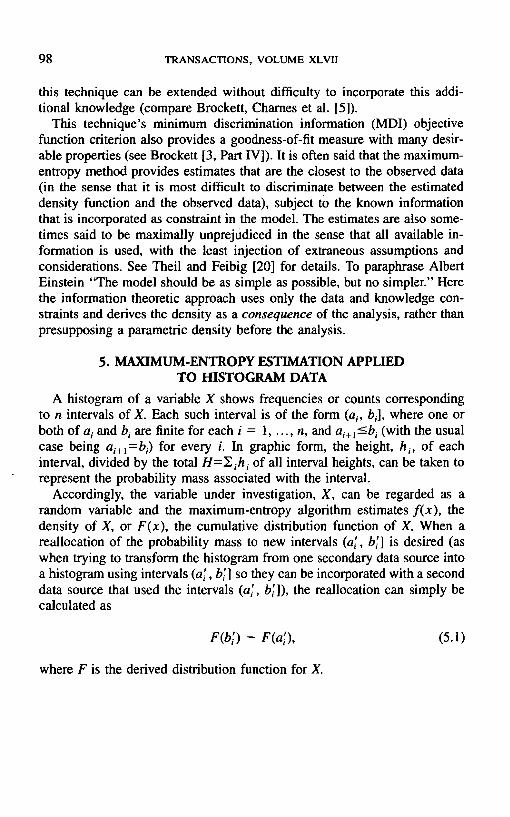
5. MAXIMUM-ENTROPY ESTIMATION APPLIED TO HISTOGRAM DATA
A histogram of a variable X shows frequencies or counts corresponding to n intervals of X. Each such interval is of the form (a;, b,.], where one or both of a i and b i are finite for each i = 1 . . . . . n, and ai÷ j <-b i (with the usual case being ai+l=bi) for every i. In graphic form, the height, h i, of each interval, divided by the total H=~,~hi of all interval heights, can be taken to represent the probability mass associated with the interval.
Accordingly, the variable under investigation, X, can be regarded as a random variable and the maximum-entropy algorithm estimates f ( x ) , the density of X, or F ( x ) , the cumulative distribution function of X. When a reallocation of the probability mass to new intervals (a~, b~] is desired (as when trying to transform the histogram from one secondary data source into a histogram using intervals (a~, b'] so they can be incorporated with a second data source that used the intervals (a~, b~]), the reallocation can simply be calculated as
F(b; ) - F(a;) , (5.1)
where F is the derived distribution function for X.
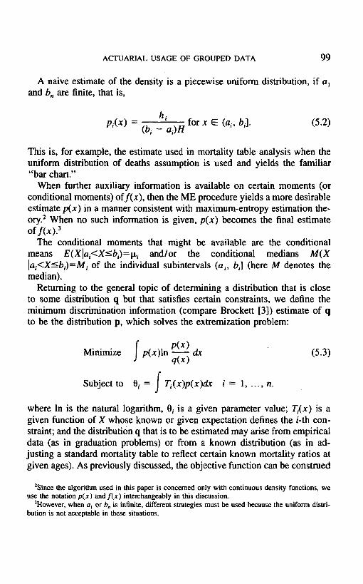
ACTUARIAL USAGE OF GROUPED DATA 99
A naive estimate of the density is a piecewise uniform distribution, if a~ and b n are finite, that is,
h i Pi(X) - for x E (a i, bi]. (5.2)
(b i - ai)H
This is, for example, the estimate used in mortality table analysis when the uniform distribution of deaths assumption is used and yields the familiar "bar chart."
When further auxiliary information is available on certain moments (or conditional moments) off(x) , then the ME procedure yields a more desirable estimate p(x) in a manner consistent with maximum-entropy estimation the- ory. 2 When no such information is given, p(x) becomes the final estimate of f (x) . 3
The conditional moments that might be available are the conditional means E(Xlai<X<-b~)=~i and/or the conditional medians M(X lai<X<-bi)=Mi of the individual subintervals (a i, bi] (here M denotes the median).
Returning to the general topic of determining a distribution that is close to some distribution q but that satisfies certain constraints, we define the minimum discrimination information (compare Brockett [3]) estimate of q to be the distribution p, which solves the extremization problem:
Minimize
Subject to
p(x) f p(x)ln - ~ ) dx
0 i = ~ Ti(x)p(x)dx d
i : 1 . . . . . n.
(5.3)
where In is the natural logarithm, 0i is a given parameter value; T,(x) is a given function of X whose known or given expectation defines the i-th con- straint; and the distribution q that is to be estimated may arise from empirical data (as in graduation problems) or from a known distribution (as in ad- justing a standard mortality table to reflect certain known mortality ratios at given ages). As previously discussed, the objective function can be construed
2Since the algorithm used in this paper is concerned only with continuous density functions, we use the notation p(x) and f ( x ) interchangeably in this discussion.
3However, when a t or b. is infinite, different strategies must be used because the uniform distri- bution is not acceptable in these situations.

100 TRANSACTIONS, VOLUME XLVII
as finding the "closest" distribution to q (in flae sense that the distribution found is least distinguishable from q; compare Brockett [3]), which is con- sistent with the known information stated in (5.3).
The analysis given in Brockett [3] implies that the optimal solution of the problem above is a density function p° of the form
q( x )e ~a,r,~) p'(x) = (5.4)
f q(t)e ~'13ir~') dt
(called the minimum discrimination information or MDI density) where [3 i are a set of parameters to be estimated in such a way that the constraints are all satisfied. Essentially, the final estimate adjusts the prior estimate q in a multiplicative manner to obtain consistency with the known information constraints.
There are now special cases to consider. First, when the distribution q(x) is a uniform density (like an "ignorance" prior in Bayesian statistics), the optimal solution p* for (5.3) is found by solving a maximum-entropy problem
f 1 Maximize p(x) In p - ~ dx
Second, when the data or standard distribution q that is to be estimated is in histogram form, q can be modeled as a piecewise-uniform density q(x), and the integral
bn
f(x) fS(x) In q-~x) dx al
in the objective function of (5.3) can be expressed as
bi
p p(x)
ai

ACTUARIAL USAGE OF GROUPED DATA 101
Each integral in this sum is equivalent (up to a constant) to a corre- sponding entropy expression over the same interval. We use this equivalency when f ( x ) must be estimated separately for each interval, rather than "systemwide."
Since the MDI statistic is additive, the estimation o f f ( x ) interval by in- terval, in fact, provides a global MDI estimate of the entire density, provided that only mass constraints are given (for example, histogram values without auxiliary information). We show below how (5.3) is developed for our piece- wise constant choice of q(x) when certain conditional means are also known for each interval in a subset I of the n intervals.
To minimize (5.3) subject to conditional mean constraints of the form
bi
f x p( x )dx ai
bi
f p( x )dx ai
= Ixi i E I, (5.5)
for that subset 1 of indices of subintervals for which this conditional mean type of information is given, we rewrite (5.5) as
bn
f (x - I.~i)ll~,. b,lP(X)dx = O, al
(5.6)
where lt~,. b,1 denotes the indicator function of the interval [a i, bi]. This can be written in the global expectation constraint formulation of (5.3) by defining
Ti(x) = f x Ix i
L 0
for a i < x <-- b i
otherwise i ~ I. (5.7)
For intervals i ~ I, we know only the mass (or histogram height) informa- tion, which can be written as

102 TRANSACTIONS, VOLUME XLVII
bl
f p( x )dx hi H '
al
(5.8)
which can also be put into the global expectational constraint form of (5.3) by defining
10 for a~ < x <- b i T~(x) = i ~ 1. (5.9)
otherwise
Note that in the numerator of (5.4), only one of the T~(x) is nonzero for any given value of x, so that we can reformulate the solution as
I q( x )ea,~-~,~ / C
f* (x ) = I,q(x) ea'lC
for x E (a i, bi], i ~ I
f o r x E ( a i, bi], i ~ I (5.10)
Here the denominator of (5.4), which can be viewed as a normalization constant, is abbreviated by the symbol C. The first expression in (5.10) is a truncated exponential conditional density, and the second expression is a uniform conditional density.
This result also encompasses cases in which (conditional) medians or, more generally, percentiles are known. Using the algebra of densities and expectations, such median knowledge merely translates into additional con- straints of the type in (5.3), with Ti(x) again defined by (5.7) or (5.9).
So far, we have shown that the maximum-entropy density over a closed interval [a, b], when no moment information is available, is the uniform density. When a mean for a similar interval is known, the maximum-entropy distribution is the truncated exponential (see Brockett, Charnes, and Paick [5] and Theil and Feibig [20]). Similarly, some other well-known special cases of (5.4) are listed in Table 3 (taken in part from Theil and Feibig [20, pp. 9]). 4
4Note the x-axis scaling on the expressions for the exponential and truncated exponential distribu- tions in the table. These density functions are usually applied to intervals with one endpoint at x=O. In analyzing histograms, it may be necessary to fit these density functions for individual intervals of x with arbitrary endpoints; for this reason the table displays the most general forms of

ACTUARIAL USAGE OF GROUPED DATA 103
TABLE 3
SUMMARY OF MAXIMUM ENTROPY DISTRIBUTION FOR DIFFERENT KNOWN INFORMATION SCENARIOS
Interval Moments Known ME Density
[a. b]
[a, bl
[42, O0]
[-ao, b]
[ - = , ool
None Mean ~,
Mean p~
Mean O,
Mean p, and Variance tr 2
Uniform: f (x ) = 1 / (b -a ) Truncated exponential: f ( x ) = a e ~ ' l ( e ~ - e *')
is an implicit function of p,. Exponential: f ( x ) = e -t~-°m'-°~l/(p,-a)
Exponential: f ( x ) = e-lV'-'~)t(b-v')ll(b-p,)
Normal: I
f(x) = ~ e - ~ ' - ~ 2,,2
6. THE HEURISTIC PROCEDURE FOR DENSITY ESTIMATION IN SOME SPECIFIC INFORMATIONAL SETI'INGS
In a given information scenario, any combination of the following may be known: the unconditional mean of f (x ) ; the unconditional median of f (x) ; and conditional (interval) means and/or medians for a number of the intervals [a i, bi]. The distributional scenarios must be treated differently for the cases of a~=-oo and/or b=oo . For brevity, in this paper we do not consider moments other than means and quantiles, because such higher-order generalized moments are unlikely to be realized from published secondary data or from subjective estimation methods (although the mathematics for accomplishing their inclusion poses no problems, for example, see Brockett [3]).
The order of precedence for the use of this information in the heuristic algorithm implemented via computer as described in this paper is as follows: If two or more interval means are known, they are used. The unconditional mean, then, is not used, nor are medians for those intervals. Any known medians for the remaining intervals are used. The unconditional median, if it is known and if it does not fall into one of the intervals for which a mean is known, is used. If only one interval mean is known and the overall mean is known, the user can choose which one to use. Any information sets not prohibited by the above rules can be used in their entirety.
the function. Also, the exponential distribution on (-oo, b] is written to be monotonically increasing. Other combinations of moments and intervals result in ME distributions that can be derived by using the same procedure demonstrated in (5.5)-(5.10).

1 0 4 TRANSACTIONS, VOLUME XLVII
A restatement may clarify these rules: If a conditional mean and median for the same interval are known, priority is arbitrarily given to the interval mean. Also, a known conditional median simply results in the splitting of an interval into two new subintervals, each with half the probability mass of the original. A known overall median likewise results in the splitting of an interval, although this will usually be an uneven division. Median-only operations always result in a new q(x), which has the same form as (6.2). From the context of the available data, no interval means will be known for these newly created intervals, but the unconditional mean still may be known and used.
The following (not all encompassing set of) illustrations provide estimates for use as building blocks for the inference of the desired but unknown true distribution function F(x) . These building blocks can then be composed 5 according to the rules given earlier in this section to obtain the desired global estimates of F. These discussions and those of Brockett [3] show how to include any and all information in the analysis if desired.
/L When the C o n d t t i o n a l M e a n f o r a B o u n d e d I n t e r v a l (a, b] Is K n o w n
The ME conditional distribution for the interval is the truncated exponen- tial. The known mean, Ix, is related to the parameter a of the exponential distribution by the equation
be etb __ a e ' ~ a -t. (6.1)
p, = e a b _ e a a
The segment of the distribution function for x~[a, b] is then
F ( x ) = F(a) + (6.2) eab - eO~ •
Now, however, we must adjust the vertical scaling because, as F ( x ) is writ- ten in (6.2), we have F ( b ) - F ( a ) = 1. To be consistent with the histogram data we started with, this quantity must be scaled upward or downward to reflect the particular interval mass h J H (if this is the i-th interval and a=a i and b=bi), which may not be unity. Accordingly, we revise F(x ) to
~These estimates assume that the user-provided moment information is correct.

ACTUARIAL USAGE OF GROUPED DATA 105
hi(e ~x -- eotal) F*(x) = F*(ai) + H ( e ~ ' _ e ~ ) for x E (a i, bi]. (6.3)
B. When the C o n d i t i o n a l M e d i a n o f (at, b~] Is K n o w n
The ME conditional distribution is piecewise-uniform in this situation. The "mass" in this interval is h i according to the histogram data. In this case (a,., bi] is split into two subintervals (ai, Mi) and (Mi, bi], each of which now is given a mass equal to h i 2 . No additional information is available for the newly created intervals, so each such subinterval j is associated with a ME distribution that is uniform on that subinterval. When x belongs to (a j, b j],
h j (x - aj) F* (x ) = F*(aj) + [H(bj - aj)]" (6.4)
C. When the U n c o n d i t i o n a l M e a n Is K n o w n a n d All S u b i n t e r v a l s Are B o u n d e d
We apply (5.3) with q(x)=hi l [H(bi -a i ) ] for xG(a i, bi] and with the con- straint set
f xp ( x )dx =
ai
bo
p ( x ) d x = 1
ai
(6.5)
The ME distribution is then a piecewise truncated exponential:
p ( x ) =
hi e - ~
H(b i - ai)
f q(t)e -~t dt
for x E (a i, bi], i = 1 . . . . . n. (6.6)
where the same limits of integration apply. Substituting (6.6) into (6.5) yields

106 TRANSACTIONS, VOLUME XLVII
~i b i - - 4- - - +
= (6.7) Ix ~ b~-a~ [ h' ] [e-a°'-e-ab']
While Equation (6.7) is not easily solvable for 13 in terms of Ix, the value of 13 can easily be obtained by numerical techniques. By integrating (6.6), where F*(a~)=0, the corresponding distribution function F*(x) can be writ- ten as
F*(x) = F*(a~) + , x E (a i, b i] (6.8)
D. When No Subinterval Moment Information Is Available f o r a Half-Unbounded Interval
This situation must be broken down into two cases: when the overall (unconditional) mean is not known and when this overall mean is known.
(1) When the Unconditional Mean Is Not Known
To be able to use the results of the previous section, the unbounded in- tervals are closed by means of an ad hoc procedure called the "rule of ten." The total width of the histogram's interior intervals is b.-a m. An exterior interval that is unbounded is given a width of ten times this quantity. For example, if both exterior intervals of the histogram are half-unbounded, the leftmost interval is given endpoints [(a m- lO(b.-am), at], and the rightmost is given endpoints [b., b.+ 10(b.-am)]. These bounded intervals are accorded uniform ME conditional densities, with distribution functions as in (6.4). The rule of ten is justified by the idea that the resulting interval widths would contain 99% of the mass of any monotonically decaying "true" den- sity function. This is a heuristic and may, of course, understate probabilities near the interior endpoint.

ACTUARIAL USAGE OF GROUPED DATA 107
(2) IVben the Uncondiu'onal Mean Is Known
The half-unbounded interval must be an exterior interval of the histogram; if n>2, it will be adjacent to a bounded interior interval. The rule used in this case is: assign a conditional mean to the half-unbounded interval such that the conditional mean of the two intervals combined is located at their mutual boundary (endpoint).
For example, suppose the histogram's rightmost interval is unbounded on the right. Its endpoints are a. and +oo. The next-to-rightmost interval is (a._ l , b._l], where b._l=a . and whose conditional mean is Ix.-I. We assign a value to Ix. such that
hn-I Ixn-I + h . Ix. h._ t + h . = an (6.14)
that is,
a. (hn_ I + h.) - h._ I Ix.-I (6.15) Ix" = h .
The conditional ME density is exponential with mean Ix.. The segment of the distribution function is
hn F*(x) = F(a.) + -~ [1 - e <a"-x)l¢~"-~")] for x E (a., oo]. (6.16)
For the opposite instance, where the leftmost interval ( i= 1) is unbounded on the left, we assign
a2(h I + h 2) - h2ix2 (6.17) Ixl = hi
whence
h F*(x) = =.! eta~-x)/t~,-a2) for x • ( - ~ , a2]. (6.18)
H
108 TRANSACTIONS, VOLUME XLVII
7. APPLICATION EXAMPLES
In this section, we apply the formulas derived in Section 6 to solve the problems posed previously.
Adjusting the Life Table by Incorporating Medical Study Resul ts
Table 1 contained the relative mortality ratios for 5,131 spinal cord injury patients by neurological category and age group at time of injury. Starting with the 1980 Standard U.S. Life Table, Brockett and Song [9] incorporated the results in Table 1 to derive an adjusted life table for calculating wrongful injury damage award compensation and for determining life insurance pre- miums for medically impaired lives by minimizing the "information dis- tance" between the adjusted life table and the standard life table subject to the applicable constraints. These constraints are formulated to fulfill the characteristics of a life table as well as the medical study results. Their method provides a way to adjust a standard life table to reflect the known characteristics of the individual while remaining as close as possible to a given standard table. Figure 2 shows the standard and adjusted survival curves for incomplete paraplegia patients.
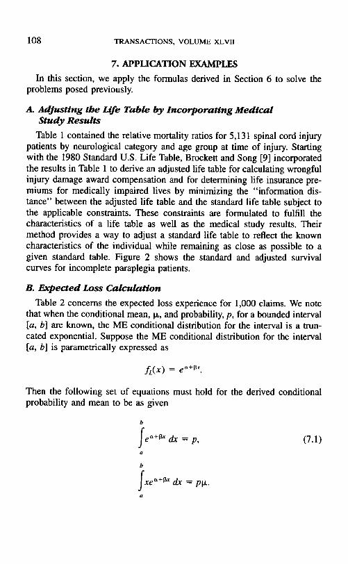
B. Expec ted Loss Calculat ion
Table 2 concerns the expected loss experience for 1,000 claims. We note that when the conditional mean, Ix, and probability, p, for a bounded interval [a, b] are known, the ME conditional distribution for the interval is a trun- cated exponential. Suppose the ME conditional distribution for the interval [a, b] is parametrically expressed as
fL(x) = e "+1~.
Then the following set of equations must hold for the derived conditional probability and mean to be as given
b
f e Q+I~' dx = p, a
b
f xe ~'+l~ dx = plx. d
(7.1)

ACTUARIAL USAGE OF GROUPED DATA
FIGURE 2
A D J U S T E D M O R T A L I T Y R A T E S BY I N F O R M A T I O N T H E O R E T I C A P P R O A C H
F O R I N C O M P L E T E P A R A P L E G I A
- l
-2
..~-3
~ - 4 ° ~
L
- ~ - 6
-7
-8
-9
f )
. . . . . . In (ip)
1 t l, , , t ~ ......
0 20 40 60 80 1 O0 120
Age
109
Transforming the equations on the previous page, we obtain
and
1 1 + p.13 -- a ~ 13 = - - In (7.2a)
b - a 1 + Ix13- b13
p13 ot = In (7.2b)
ebl3 _ eaf~"
We can then obtain the numerical results, answering any probabilistic questions concerning this example. Because Table 2 shows that the condi- tional mean for the first interval (loss=S0) is 0, all the mass (that is, 0.075) is put in one point. The parameters a and [3 for the next six bounded intervals are presented in Table 4.

110 T R A N S A C T I O N S , V O L U M E X L V I I
TABLE 4
NUMERICAL RESULTS FOR ME CONDITIONAL PROBABILITY FUNCTION
Loss Interval [a, bl ~ 13
l , lO00 - -15 .294 0 .009995 lOO1, 5000 -- 12.865 0 .000898 5001, 10000 -- 18.439 0 .000960 10001, 100000 - 1 2 . 1 2 4 - 0 .000100 1 0 0 0 0 1 , 500000 - 1 6 . 2 1 5 - 0 . 0 0 0 0 0 9 500001, 1 ~ - 16.527 - 0 . 0 0 0 0 0 5
Note that the last loss interval in Table 2 (that is, $1,000,000+) is a half- bounded interval with its conditional mean given. The results in Table 3 can then be applied to obtain the distributional function for this interval.
Based on the ME distribution obtained for this example, those questions raised in the introduction can be answered easily. For example, if it is desired to know the probability that a claim will exceed a certain threshold level, say, $50,000, and also to know the expected claim size if a policy were issued with this threshold level as a policy limit, we then calculate
P = Pr[Loss -> $50,000] = f fL (x)dx 50,000
50,000
= 1 - f fL(x)dx 0
10,000 50,0011
0 10,000
50,000
= 1 - 0 . 9 7 5 - f e- lZ124-° '~dx 10.000
= 0.0054.

ACTUARIAL USAGE OF GROUPED DATA 111
Similarly,
E[Claimlclaim limit = $50,000]
50.000 / I
= I xfL(X)dx + 50,000 Pr[Loss --> $50,000] i
0
= (0)(0.075) + (900)(0.5) + (4,000)(0.25)
+ (9,000)(0.15)
50,000
+ f xfL(xldx 10,000
+ (50,000)(0.0054)
= 0 + 450 + 1,000 + 1,350 + 378 + 270
= $3,448,
where the integral from $10,000 to $50,000 is easily obtained by calculation using the exponential formula for fL(x) over the interval.
(7. The Actuarial Software Marketer The percentages corresponding to the bars of Figure 1 were 36%, 39%,
19%, and 5%. The report stated the maximum observed number of uses was 50. It is apparent the median cannot possibly be 4.5; that would make at least 73% of the observations greater than the median. We ran the estimation several times; once without using the untrustworthy median, and also under the assumption that the 4.5 was a typographical error and the true median was 5.5, 6.5, or 7.5. It was also nature to check the feasibility of the mean. Using the endpoints of the published histogram, we can bound the mean:
0.36(0) + 0.39(5.0) + 0.19(10.0) + 0.05(30.0) = 5.4 <-- p,
-< 12.1 = 0.36(5.0) + 0.39(9.9) + 0.19(29.9) + 0.05(50.0).
A mean of 8.5 appears reasonable, and we can proceed with the estima- tion. The results are presented in Table 5.

112 TRANSACTIONS, VOLUME XLVH
TABLE 5
SENSITIVITY OF THE INFORMATION THEORETIC DISTRIBUTION ESTIMATE
OF THE PERCENTAGE OF FIRMS WITH SIXTEEN OR MORE USES
OF THE GIVEN DEFINED-BENEFIT CALCULATION AS THE SUPPLIED
MEDIAN USE CHANGES
Median
none 4.5 5.5 6.5 7.5
Number of Firms Using
0-15 Times 16 or More Times
84.6% 15.4% 84.6 15.4 83.9 16.1 84.5 15.5 85.2 14.8
The insensitivity of the far fight column to the choice of median provided some degree of comfort with the initial market estimate for the software product.
8. CONCLUDING REMARKS
The heuristic statistical procedure described in this paper (use what is known and maximize the uncertainty of what is not known) can be cate- gorized as problem-solving for grouped data with auxiliary information. Such problems arise naturally in the actuarial analysis of secondary data. Responding to data interpretation needs that arise in actuarial practice, the algorithmic portion uses available information theoretic techniques when possible. In other cases, when data are missing or in conflict, ad hoc mea- sures (based on practical logic and experience) are taken to facilitate the use of the same techniques. A variety of solved application examples were pro- vided, and further application areas indicated.
ACKNOWLEDGMENT
This paper arose in part from a problem first posed by Edward Lew at the 1984 Actuarial Research Conference in Waterloo, Ontario. The research was funded in part by a grant from the Actuarial Education and Research Fund of the Society of Actuaries. The comments of an anonymous referee are gratefully acknowledged.
REFERENCES
l. ARTHANARI, T.S., AND DODGE, Y. Mathematical Programming in Statistics. New York: Wiley, 1981.

ACTUARIAL USAGE OF GROUPED DATA 113
2. BLUM, J.R., AND ROSENBLATI', J.I. Probability and Statistics. Philadelphia, Pa.: W.B. Saunders Co., 1972.
3. BROCKETI', EL. "Information Theoretic Approach to Actuarial Science: A Unifica- tion and Extension of Relevant Theory and Applications," TSA XLIII (1991): 73-114.
4. BROCKETT, EL., CHARNES, A., GOLDEN, L., AND PAICK, K. "Constructing a Uni- modal Bayesian Prior Distribution from Incompletely Assessed Information," CCS Report #694, The University of Texas at Austin, 1993.
5. BROCKE'Vr, EL., CHARNES, A., AND PAICK, K. "Constructing a Unimodal Prior Distribution," Memoria X Congresso Academia Nacional De Ingeneria, Sonora, Mexico, pp. 145-8. Sept. 1984; Dept. of Finance, working paper 83184-2-26, Uni- versity of Texas, 1983.
6. BROCKE'rr, EL., AND COX, S.H. Discussion of Reitano, "A Statistical Analysis of Banded Data with Applications," TSA XLII (1990): 413-5.
7. BROCKEYr, EL., AND LEVlNE, A. Statistics, Probability and Their Applications, Phil- adelphia, Pa.: W.B. Saunders Co., 1984.
8. BROCKETr, EL., Ll, H., HUANG, Z., AND THOMAS, D. "Information Theoretic Mul- tivariate Graduation," SIAM Journal of Applied Mathematics, no. 2 (1991): 144-53.
9. BROCKE'rr, EL., AND SONG, Y. "Obtaining a Life Table for the Spinal Cord Injury Patients Using Medical Results and Information Theory," Journal of Actuarial Prac- tice, 3, no. l (1995): 77-92.
10. BaOCKE'rr, EL., AND ZHANG, J. "Information Theoretic Mortality Table Gradua- tion," Scandinavian Actuarial Journal (1986): 131-40.
I 1. DEVIvo, M.J., KARTUS, EL., STOVER, S.L., RLrrr, R.D., AND FINE, ER. "Seven Year Survival Following Spinal Cord Injury," Archives of Neurology, 44 (1987): 872-5.
12. HAITOVSKY, Y. "Grouped Data," in Encyclopedia of Statistical Sciences vol. 3, ed. S. Kotz and N.L. Johnson. New York: John Wiley and Sons, 1983, 527-36.
! 3. HOGG, R., AND KLUGMAN, S. Loss Distributions. New York: John Wiley and Sons, 1984.
14. KHINCHINE, A.I. Mathematical Foundations of Statistical Mechanics, New York: Dove Publishers, 1948.
15. KULLBACK, S. Statistical Information Theory. New York: Wiley, 1959. 16. KULLBACK, S., AND LEIBLER, R.A. "On Information and Sufficiency," Annals of
Mathematical Statistics, 22 (1951): 79-86. 17. RErrANO, R. "A Statistical Analysis of Banded Data with Applications," TSA XLII
(1990): 375-420. 18. SARD, A., AND WEINTRAUB, S. A Book of Splines. New York: Wiley, 1971. 19. SMITH, R.C., JR. ed. Mergers & Acquisitions Healthcare Sourcebook, 2nd ed. Phil-
adelphia, Pa.: MLR Publishing Co., 1990. 20. "I'ImlL, H., AND FEIBIG, D.G. Exploiting Continuity: Maximum Entropy Estimation
of Continuous Distributions, Cambridge, Mass.: Ballinger, 1984.