Aalborg Universitet

Trajectory Planning for Robots in Dynamic Human Environments

Svenstrup, Mikael; Bak, Thomas; Andersen, Hans Jørgen

Published in:Trajectory Planning for Robots in Dynamic Human Environments

DOI (link to publication from Publisher):10.1109/IROS.2010.5651531

Publication date:2010

Document VersionPublisher's PDF, also known as Version of record

Link to publication from Aalborg University

Citation for published version (APA):Svenstrup, M., Bak, T., & Andersen, H. J. (2010). Trajectory Planning for Robots in Dynamic HumanEnvironments. In Trajectory Planning for Robots in Dynamic Human Environments: Proceedings of theIEEE/RSJ International Conference on Intelligent Robots and Systems (IROS 2010) (pp. 4293-4298). IEEEPress. I E E E International Conference on Intelligent Robots and Systems. Proceedings, DOI:10.1109/IROS.2010.5651531

General rightsCopyright and moral rights for the publications made accessible in the public portal are retained by the authors and/or other copyright ownersand it is a condition of accessing publications that users recognise and abide by the legal requirements associated with these rights.

? Users may download and print one copy of any publication from the public portal for the purpose of private study or research. ? You may not further distribute the material or use it for any profit-making activity or commercial gain ? You may freely distribute the URL identifying the publication in the public portal ?

Take down policyIf you believe that this document breaches copyright please contact us at vbn@aub.aau.dk providing details, and we will remove access tothe work immediately and investigate your claim.

Downloaded from vbn.aau.dk on: juli 05, 2018

Trajectory Planning for Robots in Dynamic Human Environments

Mikael Svenstrup, Thomas Bak and Hans Jørgen Andersen

Abstract— This paper presents a trajectory planning algo-rithm for a robot operating in dynamic human environments.Environments such as pedestrian streets, hospital corridors,train stations or airports. We formulate the problem as planninga minimal cost trajectory through a potential field, definedfrom the perceived position and motion of persons in theenvironment.

A Rapidly-exploring Random Tree (RRT) algorithm is pro-posed as a solution to the planning problem, and a new methodfor selecting the best trajectory in the RRT, according to the costof traversing a potential field, is presented. The RRT expansionis enhanced to account for the kinodynamic robot constraints byusing a robot motion model and a controller to add a reachablevertex to the tree.

Instead of executing a whole trajectory, when planned, thealgorithm uses a Model Predictive Control (MPC) approach,where only a short segment of the trajectory is executed whilea new iteration of the RRT is computed.

The planning algorithm is demonstrated in a simulatedpedestrian street environment.

I. INTRODUCTION

As robots integrate further into our living environments,it becomes necessary to develop methods that enable themto navigate in a safe, reliable, comfortable and natural wayaround humans.

One way to view this problem is to see humans as dynamicobstacles that have social zones, which must be respected.Such zones can be represented by potential fields [1], [2].The navigation problem can then be addressed as a trajectoryplanning problem for dynamic environments with a potentialfield representation. Given the fast dynamic nature of theproblem, robotic kinodynamic and nonholonomic constraintsmust also be considered.

In the recent decade sampling based planning meth-ods have proved successful for trajectory planning [3].They do not guarantee an optimal solution, but are oftengood at finding solutions in complex and high dimensionalproblems. Specifically for kinodynamic systems Rapidly-exploring Random Trees (RRT’s), where a tree with nodescorrespond to connected configurations (vertices) of the robottrajectory, has received attention [4].

Various approaches improving the basic RRT algorithmhave been investigated. In [5], a dynamic model of the robotand a cost function is used to expand and prune the nodesof the tree. A Model Predictive Control (MPC) approach istaken, where only a small part of the trajectory is executed,

M. Svenstrup and T. Bak are with the Department of Electronic Sys-tems, Automation & Control, Aalborg University, 9220 Aalborg, Denmark{ms,tba}@es.aau.dk

H.J. Andersen is with the Department of Media Technology, AalborgUniversity, 9220 Aalborg, Denmark hja@imi.aau.dk

while a new trajectory is calculated. When expanding avertex, a random vertex and a random control input is chosen.

In [6], an approach for better choices of vertices to expand,is proposed. It is based on a reachable set of configurationsfor each vertex.

It is often desirable to run the planning algorithm in realtime, hence requiring bounded solution time. One approachis to use anytime algorithms, which initially find a quicksuboptimal solution, and then keep improving the solutionuntil time runs out [7].

Methods for incorporating dynamic environments, havealso been investigated. Solutions include extending the con-figuration space with a time dimension (C − T space), inwhich the obstacles are static [8], as well as pruning andrebuilding the tree when changes occur [9], [10].

All these result only focus on avoiding collisions withobstacles. However, there have been no attempts to navigatethrough a human crowd taking into account the dynamics ofthe environment and at the same time generate comfortableand natural trajectories around the humans. E. Hall [11] hasanalysed how people position themselves socially relative toeach other. He divides the area around a person into fourzones (public, social, personal and intimate). These zonescan be used to plan how a robot should move to make themotion natural and comfortable.

In this paper will formulate the problem of navigatingthrough a dynamic human environment, as planning a tra-jectory through a potential field. The overall mission of therobot is, to move forward through the environment with adesired average speed and direction, which can be set by atop level planner. This paper contributes by enhancing thebasic RRT planning algorithm to accommodate for naviga-tion in a potential field and take into account the kinodynamicconstraints of the robot. The RRT is expanded using a controlstrategy, which ensures feasibility of the trajectory and abetter coverage of the configuration space. The planning isdone in C−T space using an MPC scheme to incorporate thedynamics of the environment. To be able to run the algorithmon-line, the anytime concept is used to quickly generate apossible trajectory. The RRT keeps being improved until anew trajectory is required by the robot, which can happen atany time.

The trajectory planning problem is formulated in SectionII, and the algorithm for generating the trajectory is describedin Section III. Finally in Sections IV-V the algorithm isdemonstrated in an experiment, where the robot plans thetrajectory through a simulated pedestrian street.

The 2010 IEEE/RSJ International Conference on Intelligent Robots and Systems October 18-22, 2010, Taipei, Taiwan

978-1-4244-6676-4/10/$25.00 ©2010 IEEE 4293

II. TRAJECTORY GENERATION PROBLEM

A. Robot Dynamics

The robot is modelled as a unicycle type robot, i.e. like aPioneer, an iRobot Create or a Segway. A good motion modelfor the robot is necessary because it operates in dynamicenvironments, where even small deviations from the expectedtrajectory may result in collisions. So instead of using apurely kinematic robot model of the robot, it is modelled as adynamical system, with accelerations as input. This describesthe physics better, since acceleration and applied force areproportional. This dynamical model can be described by thefive states:

x(t) =

x1(t)x2(t)x3(t)x4(t)x5(t)

=

x(t)y(t)v(t)θ(t)θ(t)

→ x position→ y position→ linear velocity→ rotation angle→ rotational velocity

(1)

The differential equation governing the robot behaviour is:

x(t) = f (x(t),u(t)) =

x(t)y(t)v(t)θ(t)θ(t)

=

v(t) cos(θ(t))v(t) sin(θ(t))

uv(t)θ(t)uθ(t)

=

x3(t) cos(x4(t))x3(t) sin(x4(t))

u1(t)x5(t)u2(t)

(2)

where u1 = uv is the linear acceleration input and u2 = uθis the rotational acceleration input.

Without loss of generality the starting time can be set to0, and the trajectory is then calculated as:

x(t) = x(0) +∫ t

0

f (x(τ),u(τ)) dτ (3)

B. Dynamic Potential Field

The value of the potential field, denoted G, at a point inthe environment is calculated as a sum of the cost associatedwith three different aspects:

1) A cost related to the robots position in the environmentwithout obstacles. For example high costs might beassigned close to the edges.

2) A cost associated with the robot position relative tohumans in the area.

3) A cost rewarding moving towards a goal.The combined cost can be written as:

G(t) = g1(x(t))) + g2(x(t),P(t)) + g3(x(t)) . (4)

P(t) is a matrix containing the position and orientation ofpersons in the environment at the given time. g1(x), g2(x)and g3(x) are the three cost functions. They are furtherdescribed below.

1) Cost related to environment: This cost function iscurrently designed for non agoraphobic behaviour of therobot, i.e. in open spaces, such as a pedestrian street. It hasthe shape of a valley, such that it is more expensive to gotowards the sides, but cheap to stay in the middle:

g1(x(t)) = cyy2(t) (5)

where cy is a constant determining how much the robot isdrawn towards the middle.

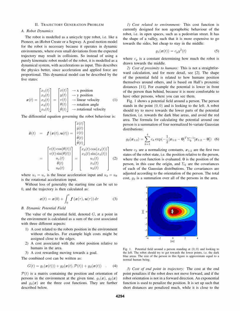
2) Cost of proximity to humans: This is not a straightfor-ward calculation, and for more detail, see [2]. The shapeof the potential field is related to how humans positionthemselves around others, and is based on Hall’s proxemicdistances [11]. For example the potential is lower in frontof the person than behind, because it is more comfortable tohave other persons, where you can see them.

Fig. 1 shows a potential field around a person. The personstands in the point (0, 0) and is looking to the left. A robotshould try to move towards the lower parts of the potentialfunction, i.e. towards the dark blue areas, and avoid the redarea. The formula for calculating the potential around oneperson is a summation of four normalized bi-variate Gaussiandistributions:

g2(x1:2) =4∑k=1

ck exp(−12

[x1:2 − 0]TΣ−1k [x1:2 − 0]) (6)

where ck are a normalizing constants, x1:2 are the first twostates of the robot state, i.e. the position relative to the person,where the cost function is evaluated. 0 is the position of theperson, in this case the origin, and Σk are the covariancesof each of the Gaussian distributions. The covariances areadjusted according to the orientation of the person. The totalcost, g2 is a summation over all of the persons in the area.

Fig. 1. Potential field around a person standing at (0, 0) and looking tothe left. The robot should try to get towards the lower points, i.e. the darkblue areas. The size of the person in this figure is approximate equal to anormal human being.

3) Cost of end point in trajectory: The cost at the endpoint penalizes if the robot does not move forward, and if therobot orientation is not in a forward direction. An exponentialfunction is used to penalize the position. It is set up such thatshort distances are penalized much, while it is close to the

4294

same value for larger distances, i.e. it does not change muchif the robot goes 19 or 20 meters from its starting position.

g3(x(t)) = ce1 exp(ce2(x(t)− x(0))) + cθθ4(t) , (7)

where c(·) are scaling constants and x(0) is the desiredposition at t = 0. The reason that θ is raised to the fourth,is to keep the term closer to zero in a larger neighbourhoodof the origin. This means that the robot will almost not bepenalized for small turns. On the other hand larger turns, likegoing the wrong way, will be penalized more.

C. Minimization Problem

Given the above cost functions a potential landscape maybe formed. Fig. 2 illustrates an example of a pedestrian streetlandscape with five persons. The robot is initially positionedat position (2, 0) and has to move to the right. The areais bounded to be 20m wide, i.e. 10m to each side of therobot from the initial position. Examples of three differentrandomly chosen trajectories are shown in the figure.

[m]

[m]

0 5 10 15 20 25 30 35 40 45−10

−5

0

5

10

Fig. 2. Person potential field landscape, which the robot has to movethrough. The robot starting point is the green dot at the point (2, 0). Threeexamples of potential robot trajectories are shown.

At a first glance it looks like all three trajectories wouldrun into at least one human, but since the persons movewhile the robot advances along the trajectory, this might notbe the case. Conversely the robot may also run into a person,who was not originally on the path. Therefor it is importantto take into account the dynamics of the obstacles (i.e. thehumans), when planning trajectories.

If the current time is t = 0, the planning problem canbe posed as follows. Given an initial robot state x0, andtrajectory information for all persons until the given timePstart:0. Determine the control input u0:T , which minimizesthe cost of traversing the potential field, subject to thedynamical robot model constraints:

minimize I(u0:T ) = (8)Z T

0[g1(x(t)) + g2(x(t),P(t))] dt + g3(x(T ))

s.t. x(t) = f (x(t),ut)

where g1(x(t)) = cyx2(t)2

g2(x(t),P(t)) =pXj=1

4Xk=1

ck exp(−1

2[x1:2 − µj ]TΣ−1

j,k[x1:2 − µj ])

g3(x(T )) = ce1 exp(ce2(x1(T )− x1(0))) + cθx44(T ),

were x1:2 = [x1(t), x2(t)] is the position of the robot attime t, u0:T is the discrete input sequence to the robot. Tis the ending time horizon of the trajectory, gx(·) are costfunctions and p is the number of persons in the area. Theposition and orientation of all persons at time t is given byP(t) and µj is the center of the j-th person at a given time.

To be able to calculate the cost of a trajectory accordingto Eq. (8), only the person trajectories remains to be de-fined. A simple model is that the person will continue withthe same speed and direction [12]. More advanced humanmotion models could be used without changing the planningalgorithm, but it is outside the scope of this paper to derivea complex human motion model.

III. RRT BASED TRAJECTORY PLANNING

The structure of the planning algorithm can be seen inFig.3. The idea is that while a trajectory is executed, a newis calculated on-line. Input to the trajectory planner is theprevious best trajectory, the person trajectory estimates, andthe dynamic model of the robot.

Execute Trajectory in Real World

Seed Tree Find Nearest Vertex

RRT Trajectory Planner

Pick Best Trajectory

Estimate Person Trajectories

Dynamic Robot Model

Sample Random

Point

Extend Tree

T < Tplanning

T ≥ Tplanning

Fig. 3. The overall structure of the trajectory generator. The blue realworld part and the red trajectory planning part are executed simultaneously.

The minimization problem stated in Eq. (8) is addressedby RRT’s. A standard RRT algorithm is shown in Algorithm1, where the lines 4, 5, 6 correspond to the three blocks inthe larger RRT Trajectory Planner box in Fig. 3.

The method presented here differs from the standardRRT in lines 1, 3, 6, 9, which are marked red. Furthermore,between line 6 and 7, node pruning is introduced. Since anMPC scheme is used, only a small portion of the plannedtrajectory is executed, while the planner is restarted to plana new trajectory on-line. When the small portion has beenexecuted, the planner has an updated trajectory ready. Tofacilitate this, the stopping condition in line 3 is changed.When a the robot needs a new trajectory, or when certainmaximum number of vertices have been extended, the RRTis stopped. Even though the robot only executes a small partof the trajectory, the rest of the trajectory should still be valid.Therefore, in line 1, the tree is seeded with the remainingtrajectory.

In line 9 the trajectory with the least cost is returned,instead of returning the trajectory to the newest vertex. The

4295

Algorithm 1 Standard RRT (see [13])RRTmain()

1: Tree = q.start2: q.new = q.start3: while Dist(q.new , q.goal) < ErrTolerance do4: q.target = SampleTarget()5: q.nearest = NearestVertex(Tree , q.target)6: q.new = ExtendTowards(q.nearest,q.target)7: Tree.add(q.new)8: end while9: return Trajectory(Tree,q.new)

SampleTarget()1: if Rand() < GoalSamplingProb then2: return q.goal3: else4: return RandomConfiguration()5: end if

tree extension function and the pruning method are describedbelow.

A. RRT Control Input SamplingWhen working with nonholonomic kinodynamic con-

strained systems, it is not straightforward to expand thetree towards a newly sampled point in the configurationspace (line 6 in Algorithm 1). It is a whole motion plan-ning problem in itself to find inputs, that drive the robottowards a given point [14]. The algorithm proposed hereuses a controller to turn the robot towards the sampled pointand to keep a desired speed. A velocity controller is setto control the speed towards an average speed around areference velocity. The probabilistic completeness of RRT’sin general, is ensured by the randomness of the input. Soto maintain this randomness in the input signals, a randomvalue sampled from a Gaussian distribution is added to thecontroller input. The velocity controller is implemented asa standard proportional controller. The rotation angle is asecond order system with θ and θ as states, and therefore astate space controller is used for control of the orientation.The control input can be written as:

u =

»u1

u2

–=

»kv(µv − v(t))

kθ1(φpoint − θ(t))− kθ2θ

–+

»N (0, σv)N (0, σθ)

–. (9)

µv is the desired average speed of the robot and φpoint is theangle towards the sampled point. k(·) are controller constantsand σv, σθ are the standard deviations of the added Gaussiandistributed input.

The new vertex to be added to the tree is now found byusing the dynamic robot motion model and the controller tosimulate the trajectory one time step. This ensures that theadded vertex will be reachable.

B. Tree Pruning and Trajectory Selection

A simple pruning scheme, based on several differentproperties of a node, is used. If the vertex corresponding tothe node ends up in a place where the potential field has avalue above a specific threshold, then the node is not added tothe tree. Furthermore a node is pruned if |θ(t)| > π

2 , whichmeans that the robot is on the way back again, or if the

simulated trajectory goes out of bounds of the environment.It is not desirable to let the tree grow too far in time, sincethe processing power is much better spend on the near future,because of the uncertainty of person positions further into thefuture. Therefore the node is also pruned if the time taken toreach the node is above a given threshold. Finally, instead ofreturning the trajectory to the vertex of the last added node,the trajectory with the lowest cost (calculated from Eq. (8)),is returned. But to avoid the risk of selecting a node, whichis not very far in time, all nodes with a small time are thrownaway before selecting the best node.

The final algorithm is shown in Algorithm 2.

Algorithm 2 Modified RRT for human environmentsRRTmain()

1: Tree = q.oldBestTrajectory2: while (Nnodes < maxNodes) and (t < tMax) do3: q.target = SampleTarget()4: q.nearest = NearestVertex(Tree , q.target)5: q.new = CalculateControlInput(q.nearest,q.target)6: if PruneNode(q.new) == false then7: Tree.add(q.new)8: end if9: end while

10: return BestTrajectory(Tree)SampleTarget()

1: if Rand < GoalSamplingProb then2: return q.goal3: else4: return RandomConfiguration()5: end if

IV. SIMULATIONS

The above described algorithm is implemented, anddemonstrated to work on a simulated pedestrian street, asshown in Fig. 2. The experiments consist of two parts.First, the algorithm is applied on the environment shownin Fig. 2. This will demonstrate that the algorithm is capableof planning a trajectory, which does not collide with anypersons. It will also demonstrate how the tree expands. Thealgorithm is compared to an algorithm where a randomvertex and a random control input is chosen, as suggestedin [4] and used to different extends in e.g. [5], [6]. Next,a simulated navigation through several randomly generatedworlds is performed. This will demonstrate the robustness ofthe algorithm over time.

The following parameters for the potential field are used:cy = 0.1, ce1 = 20, ce2 = −0.1, cθ = 10, and the parametersfor the Gaussian distributions can be seen in [2]. The polesof the controllers, the reference velocity and the standarddeviation of the velocity input, are the only other parametersto set. The poles have experimentally been determined, suchthat the robot has a relatively quick response, but the exactpole placement does not influence the trajectory generationmuch. The pole of the velocity controller is placed in s =

4296

−2, and both the poles of the rotational controller are placedin s = −2 as well. The standard deviation of the addedrandom velocity input is set to σv = 2ms and the standarddeviation of the rotational input is set to σθ = 0.5 rads . Thereference velocity is set to 1.5ms , which is considered as anormal human walking speed.

A. Robustness Test

The robustness test is performed in 50 different randomlygenerated environments, where the robot has to navigateforwards in one minute. With an average speed of 1.5ms , thiscorresponds to the robot moving approximately 90m aheadalong the street. In each simulation the robot’s initial stateis:

x0 = [2 0 0 0 0]T (10)

First the motion of all the persons in the world are simulated.Initially a random number of persons (between 10 and 20)are placed randomly in the world. Their velocity is sampledrandomly from a Gaussian distribution. The motion of eachperson is simulated as moving towards a goal 10m aheadof them. The goal position of the y − axis of the street issampled randomly, and will also change every few seconds.Additional Brownian motion is added to each person toinclude randomness of the motion. Over time new personswill enter at the end of the street according to a Poissonprocess. This means that at any given time, persons willappear and disappear at the ends of the street. Because ofthis randomness, the number of persons can differ from theinitial number of persons, and ranges from 10 to around 40,which is different for each simulation.

At each time instant, the robot will only know the currentposition and velocity of each of the persons within a rangeof 45m in front of the robot, and it has no knowledge aboutwhere the persons will go in the future.

As it is a simulation, there is no real time performanceissues, and nothing has been done to optimize the code forfaster performance. So the tree is set to grow a fixed numberof 2000 vertices at each iteration. The planning horizon isset to 20 seconds and at each iteration the robot executes 2seconds of the trajectory, while a new trajectory is planned.

V. RESULTS

An example of a grown RRT, with 2000 vertices, from theinitial state can be seen in Fig. 4. The simulated trajectoriesof the robot are the red lines, and the red dots are verticesof the tree. It is seen how the RRT is spread out to explorethe configuration space, although only every 10th vertex isplotted to avoid clutter on the graph. Note that the personsare static at their initial position on the figure, and sometrajectories seem to pass through persons. But in reality, thepersons have moved when the robot passes the point of thetrajectory. The best of the all trajectories, which is calculatedusing Eq. (8), is the green trajectory.

In Fig. 5 a RRT has been run for the same environment,but by choosing a random vertex to expand, instead of theone closest to a random sampled point. The algorithm is alittle faster, since it does not have to calculate distances to all

[m]

[m]

0 5 10 15 20 25 30 35 40 45−10

−5

0

5

10

Fig. 4. An RRT for a robot starting at (2, 0) and the task of movingforward through the human populated environment. Only every 10th vertexis shown to avoid clutter of the graph. The vertices are the red dots, andthe lines are the simulated trajectories. The green trajectory is the least costtrajectory.

vertices. But as can be seen, the tree does almost not expandover the configuration space.

[m]

[m]

0 5 10 15 20 25 30 35 40 45−10

−5

0

5

10

Fig. 5. The RRT after 2000 expansions, where a random vertex is chosento be expanded. The tree expands very slow over the configuration space.The lowest cost trajectory is shown in green.

An example of the tree after 2000 expansions, whenchoosing the nearest vertex, but using a random controlinput , is illustrated in Fig. 6. The configuration space is notcovered very well, since there are only two major branchesof the tree, and the top area above the first person has notbeen explored at all. When comparing to Fig. 4, it is clearthat our control sampling method covers the configurationspace much better.

[m]

[m]

0 5 10 15 20 25 30 35 40 45−10

−5

0

5

10

Fig. 6. An example of choosing random control input. The tree expandsbetter than if choosing random nodes, but it still does not cover theconfiguration space very well. The lowest cost trajectory is shown in green.

In Fig. 7 a typical scene from one of the 50 simulationscan be seen. The blue dots are persons, and the arrows are

4297

velocity vectors, with a length proportional to the speed.The black star with the red arrow, is the robot position andorientation.

15 20 25 30 35 40 45 50 55−10

−5

0

5

10Time: 13.5s Number of persons: 39

Distance [m]

Dis

tanc

e [m

]

Fig. 7. A scene from one of the 50 simulations. The blue dots are persons,with their corresponding current velocity vectors. The black star is the robot.

In none of the 50 simulations the robot ran into a person.This demonstrates that the algorithm is robust enough tohandle simulated human motion with changing goals andadditional random motion, even though using the simplehuman motion model when planning. A few close passesin the combined 50 minute run, down the pedestrian street,are seen. But, as seen in Fig. 8, the robot stays out of thepersonal zone of any of the persons in more than 97.5% ofthe time, and out of the intimate zone (a distance closer than0.45m) 99.7% of the time. This only occurs on 9 separateinstances of the 50 minutes of driving.

Intimate Personal Social Public 0

10

20

30

40

50

60

time

in %

Zones

0.3 %d ≤ 0.45 m

2.2 %0.45 m < d ≤ 1.20 m

45.7 %1.20 m < d ≤ 3.60 m 54.8 %

d > 3.60 m

Fig. 8. The bar plot shows how large a part of the time the closest personto the robot has been in each zone. The robot should try to stay out of thepersonal and intimate zones. The distance interval for each zone, can alsobe seen in the plot.

Except in very densely populated environments, the modelruns approximately one third of real time on a 2.0 GHz CPUrunning MATLAB. This is considered to be reasonable, sinceno optimization for speed has been done.

In very dense environments, the planning takes longer,since many new added vertices, are pruned again, and hencemore points has to be sampled before 2000 vertices areexpanded. Additionally the more persons in the area, thelonger it takes to evaluate the cost of traversing the potentialfield.

On average approximately 14 of the sampled points led

to an expansion of the tree and correspondingly 34 led to a

pruned node.

VI. CONCLUSIONS

In this paper a new algorithm for trajectory planning fora kinodynamic constrained robot, has been described. Therobot is navigating in a highly dynamic environment, whichin this case is populated with humans. The algorithm is basedon RRT’s, but with a new trajectory selection method. Themethod enables the costs of traversing a potential field to beminimized, thereby supporting planning of comfortable andnatural trajectories. Further, a new control input samplingstrategy has been presented. This leads to better tree coverageover the configuration space, than if sampling e.g. a randomcontrol input. Together with a dynamic model of the robot,an MPC scheme is used to enable the planner to continuouslyplan a reachable trajectory on an on-line system.

The algorithm is challenged when the environments be-come very densely populated, but so are humans. Humansreact by mutual adaptation and allowing violation of thesocial zones. This is not done here, where the robot takeson all the responsibility for finding a trajectory.

Potential future work include real life experiments, andincorporation of human to human motion correlation intothe algorithm.

REFERENCES

[1] E. Sisbot, A. Clodic, L. Marin U., M. Fontmarty, L. Brethes, andR. Alami, “Implementing a human-aware robot system,” in The 15thIEEE International Symposium on Robot and Human InteractiveCommunication, 2006. ROMAN 2006., 6-8 Sept. 2006, pp. 727–732.

[2] M. Svenstrup, S. T. Hansen, H. J. Andersen, and T. Bak, “Poseestimation and adaptive robot behaviour for human-robot interaction,”in Robotics and Automation, 2009. ICRA ’09. IEEE InternationalConference on, Kobe, Japan, May 2009, pp. 3571–3576.

[3] S. LaValle, Planning algorithms. Cambridge Univ Pr, 2006.[4] S. LaValle and J. Kuffner Jr, “Randomized kinodynamic planning,”

The International Journal of Robotics Research, vol. 20, no. 5, p.378, 2001.

[5] A. Brooks, T. Kaupp, and A. Makarenko, “Randomised mpc-basedmotion-planning for mobile robot obstacle avoidance,” in Robotics andAutomation, 2009. ICRA ’09. IEEE International Conference on, May2009, pp. 3962–3967.

[6] A. Shkolnik, M. Walter, and R. Tedrake, “Reachability-guided sam-pling for planning under differential constraints,” in Robotics andAutomation, 2009. ICRA ’09. IEEE International Conference on, May2009, pp. 2859–2865.

[7] D. Ferguson and A. Stentz, “Anytime, dynamic planning in high-dimensional search spaces,” in Proc. IEEE International Conferenceon Robotics and Automation, 2007, pp. 1310–1315.

[8] J. van den Berg, “Path planning in dynamic environments,” Ph.D.dissertation, Ph. D. dissertation, Universiteit Utrecht, 2007.

[9] D. Ferguson, N. Kalra, and A. Stentz, “Replanning with rrts,” in Proc.IEEE International Conference on Robotics and Automation ICRA2006, 2006, pp. 1243–1248.

[10] M. Zucker, J. Kuffner, and M. Branicky, “Multipartite rrts for rapidreplanning in dynamic environments,” in Proc. IEEE InternationalConference on Robotics and Automation, 2007, pp. 1603–1609.

[11] E. T. Hall, “A system for the notation of proxemic behavior,” Americananthropologist, vol. 65, no. 5, pp. 1003–1026, 1963.

[12] A. Bruce and G. Gordon, “Better motion prediction for people-tracking,” in Robotics and Automation, 2004. ICRA ’04. IEEE Inter-national Conference on, April 2004.

[13] D. Ferguson and A. Stentz, “Anytime rrts,” in Proc. IEEE/RSJ In-ternational Conference on Intelligent Robots and Systems, 2006, pp.5369–5375.

[14] B. Siciliano and O. Khatib, Handbook of Robotics. Springer-Verlag,Heidelberg, 2008.

4298